1

HOURLY BIOMASS BURNING EMISSIONS INVENTORY DERIVED FROM GOES DATA

Xiaoyang Zhang Earth Resources Technology, Inc. at NOAA/NESDIS/STAR, 5200 Auth Road, Camp Springs, MD

20746 Xiaoyang.Zhang@noaa.gov

Shobha Kondragunta NOAA/NESDIS/STAR, 5200 Auth Road, Camp Springs, MD 20746

Shobha.Kondragunta@noaa.gov M. K. Rama Varma Raja

I.M. Systems Group, Inc., at NOAA/NESDIS/STAR, 5200 Auth Road, Camp Springs, MD 20746 ABSTRACT This study uses satellite data to derive biomass burning emissions in near real time across the Continuous United States (CONUS). The algorithm developed depends on key inputs of fuel loadings, burned areas, and emission and combustion factors. The fuel loading (1 km) was developed from Moderate-Resolution Imaging Spectroradiometer (MODIS) data including land cover type, vegetation continuous field, and monthly leaf-area index. The weekly fuel moisture category was retrieved from AVHRR (Advanced Very High Resolution Radiometer) Global Vegetation Index (GVIx) data for the determination of fuel combustion efficiency and emission factor. The burned area was simulated using half-hourly fire sizes obtained from the GOES (Geostationary Operational Environmental Satellites) Wildfire Automated Biomass Burning Algorithm (WF_ABBA) fire product. By integrating all these parameters, we estimate quantities of PM2.5 (particulate mass for particles with diameter < 2.5 μm), CH4, CO, N2O, NH3, NOX, SO2 and TNMHC every half hour since 2002. We further investigate spatial and temporal variations in biomass burning emissions for these species and statically analyze the dependences of fire emissions on drought conditions. The results show that emissions present significant diurnal and seasonal patterns. The month with largest emissions varies greatly in different states, although total emission across CONUS is largest in summer. Moreover, biomass burning emission is critically associated with drought, which increases exponentially with the decrease of monthly precipitation during dry seasons. INTRODUCTION Biomass burning releases trace gases and aerosols, which play a significant role in atmospheric chemistry. These contribute significantly to the uncertainty in climate change1, and affect both local and global air quality which impacts human health and environment2,3,4,5. The emissions released from biomass burning, therefore, have recently emerged as an important research topic. Emissions from biomass burning are modeled from various parameters, particularly, fuel loading and burned area. Fuel loading is a very complex parameter, so it is one of the main sources of uncertainty in emission estimates. The commonly used fuel loadings include static values in large scales6,7,8, field measurements in local areas, ecoregions-based representatives in regional areas9. The most widely used fuel data in the Continuous United States (CONUS) are derived from National Fire Danger Rating System (NFDRS)10, which are associated with fuel models using in a lookup table. A similar fuel dataset is the Fuel Characteristic Classification System (FCCS)11, which provides much detailed types of ecosystems and fuel types. The quality of such fuel data depends greatly on the class schemes of ecoregions and the representatives of fuel values. Burned area is another major parameter in emissions modeling. It is generally derived from local and national fire services or agencies in investigating historical fire emissions12. Recently, satellite

2

observations have provided a means to monitor burned areas with more accurate spatiotemporal patterns. Particaly, fire-counts from various satellites, such as the Along Track Scanning Radiometer (ATSR), the Advanced Very High Resolution Radiometer (AVHRR), and the Moderate Resolution Imaging Spectroradiometer (MODIS) have been used as a proxy for the investigation of biomass burning in near real time and past years13,14. However, the fire pixel counts are difficult to be converted to burned area accurately because satellite can usually detects the fire occurrences in much small size than the pixel in the moderate and coarse resolution data. Furthermore, the instantaneous observations from AVHRR and MODIS may miss detections of some small fire events. On the other hand, burn scars detected from time series of satellite observations (such as MODIS) demonstrate great potential for emission calculations in the past15, but they can not be applied to calculate real (near-real) time burning emissions. Alternatively, Geostationary Operational Environmental Satellites (GOES) are demonstrated to be able to estimate smoke aerosol emissions in nearly real time for forecast because of the high temporal observations16,17. This research uses multiple satellite instruments to retrieve spatially-distributed parameters for the estimates of emissions including PM2.5 (particulate matter with diameters less than 2.5µm), CH4, CO, N2O, NH3, NOX, SO2, and TNMHC. Particularly, a new fuel dataset is developed from MODIS land cover type, leaf area index (LAI), and vegetation percent cover at a spatial resolution of 1 km. Burned area is simulated from fire sizes obtained from GOES WF_ABBA (Wildfire Automated Biomass Burning Algorithm) fire product with a half-hour interval. The combustion and emission factors are associated with fuel moisture derived from AVHRR vegetation health condition. Based on these inputs, biomass burning emissions are estimated every half hours from 2002-2006 across CONUS. Temporal and spatial patterns in emissions are further investigated and their dependences on drought conditions are analyzed. Finally, the biomass burning emissions are evaluated by comparing CO concentrations derived from CMAQ (Community Multiscale Air Quality Modeling System) with AIRS (Atmospheric Infrared Sounder), where CMAQ model is run with and without GOES fire emissions.

METHODOLOGY MODELING BIOMASS BURNING EMISSIONS Biomass burning emissions are generally modeled using four fundamental parameters. These parameters are burned area, fuel loading (biomass density), the fraction of combustion, and the factors of emissions for trace gases and aerosol. By integrating these parameters, biomass burning emissions can be estimated2:

ABCFE = (1) where E represents the emissions from biomass burning (ton); A is the burned area (ha); B is the biomass density (ton/ha); C is the fraction of biomass consumed during a fire event; and F is the factor of the consumed biomass released as trace gases and smoke particulates. This simple model has been widely used to estimate the emissions in regional and global scales1,14,18. Fuel loading in this study is basically divided into live fuel loading and dead fuel loading. The live fuel loading consists of foliage and branch biomass in forests, shrub biomass, and grass (including crop) biomass. The dead fuel loading is composed of litter and coarse woody detritus. The fuel loading for each pixel was obtained from a MODIS Vegetation Property-based Fuel System (MVPFS). This dataset was primarily calculated from percent vegetation cover in MODIS continuous field product, LAI, and land cover types at a spatial resolution of 1 km19,20. Burned area was derived from NOAA GOES WF_ABBA fire product. The WF_ABBA detects instantaneous fire sizes in subpixels using 3.9 µm and 10.7 µm infrared bands by locating and characterizing hotspot pixels from a 4 km resolution of GOES data16. This product provides time of fire occurrences, fire location in latitude and longitude, instantaneous estimates of subpixel fire size, and quality assurance flags of the fire detections. The fire size is only retrieved for pixels with best quality but not for the fire pixels that are saturated, cloudy, and with high, medium, or low probabilities. To

3

minimize false fires, the WF_ABBA product uses a temporal filter to exclude the fire pixels that are only detected once within the past 12 hours. GOES fire size was empirically converted to burned area21. Specifically, by examining diurnal variability of GOES instantaneous subpixel fire sizes, representatives of diurnal fire sizes were established for a variety of ecosystems across CONUS. The corresponding representative diurnal curve was adjusted to fit fire sizes in each fire pixel detected from GOES satellite. The fitted model was employed to empirically simulate burned areas based on the formula that was established by analyzing GOES fire sizes and Landsat ETM+-based burn scars. Using this algorithm, burned areas were calculated every half hour. The half-hourly data were aggregated to hourly data suitable to air quality modeling. The factors of combustions and emissions are controlled by fuel moisture condition. The moisture is divided into six categories which are very dry, dry, moderate, moist, wet, and very wet, using AVHRR vegetation health index. These moisture conditions were applied to modify combustion factors for various fuel types.22.

The factors of PM2.5 emissions also vary with moisture conditions. The variation is generally slight for various moisture conditions based on a First Order Fire Effects Model (FOFEM)23. However, the value for coarse wood is more sensitive to moisture conditions than those for other fuel types. In this study, emission factors were obtained from FOFEM for PM2.5, CH4, CO, N2O, NH3, NOX, SO2, and TNMHC. EVALUATION OF BIOMASS BURNING EMISSION

The estimates of GOES biomass burning emissions were evaluated using CO retrieved from Atmospheric Infrared Sounder (AIRS). AIRS CO is retrieved from infrared channels in 4.58-4.50 microns24, which mainly comes from the layer close to 500 mb level. These data used here were obtained from level 2 support product with a horizontal spatial resolution of 3 degree grid (approximately 300 km). The value represents total CO concentration (contributions from both fire emissions and background values in the atmosphere in a sample) in a sample of 50 km size close to the center of 3 degree grid.

The estimates of biomass burning emissions only provide fire contribution of CO, which is hard to be directly compared with AIRS CO. Therefore, the column-integrated CO was estimated from CMAQ (Community Multiscale Air Quality Modeling System) for the comparison. The CMAQ model was processed at a spatial resolution of 12 km with 22 discrete vertical sigma layers. To study the impacts of fire emissions on CMAQ CO, CMAQ air quality model was run in base case and fire case (adding GOES fire emission inventory as input), separately.

The coincident pairs of AIRS and CMAQ CO data over CONUS domain were extracted for comparisons between June 25 and 27, 2005. In particular, CMAQ model runs with a time step of one hour and denotes the beginning of the time. This offset of downstream time is taken as the CMAQ reference time for coincident pair formation. All the CMAQ estimates within 0.5 degree radius of AIRS footprint were averaged to generate the mean value for comparison. Corresponding AIRS CO observations were selected in the time within half hour of CMAQ CO estimates. TEMPORAL AND SPATIAL ANALYSIS OF EMISSIONS Spatial and temporal patterns were statistically analyzed for emissions from 2002 to 2006. The standard statistical parameters used here include mean values, standard deviation, coefficient of variation (CV) which is defined as the ratio between standard deviation and mean value. Hourly emissions were averaged from the data during the five years to explore diurnal patterns. Similarly, monthly emissions were calculated to investigate the seasonality. Spatial variation was determined using emissions in each state across CONUS. In doing this, we identified the month with the largest emissions from biomass burning during a year for each individual state. This month was referred to as the severe emission month within a year. The median of the identified months during the five years was assumed to be the severest month in a given state.

4

Moreover, we calculated average annual emission for each state, separately, to detect the spatial variation. Biomass burning emissions from wildfire are impacted by weather conditions, particularly drought. Therefore, the relationship between seasonality of biomass burning emissions and precipitation was further investigated. In doing so, precipitation data were obtained from 3-hourly precipitation data at a spatial resolution of 32 km between 2002 and 2006 from the NCEP (National Centers for Environmental Prediction) North America Regional Reanalysis (NARR)25. This dataset was produced using a fixed assimilation/forecast model and is the most accurate and consistent long-time series of dataset that covers the entire North America. We explored the dependence of emissions on drought by analyzing monthly biomass burning emissions and precipitation for each state across CONUS. RESULTS COMPARISON OF BIOMASS BURNING EMISSIONS WITH AIRE CO

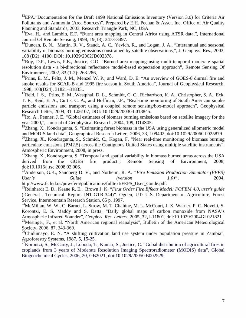
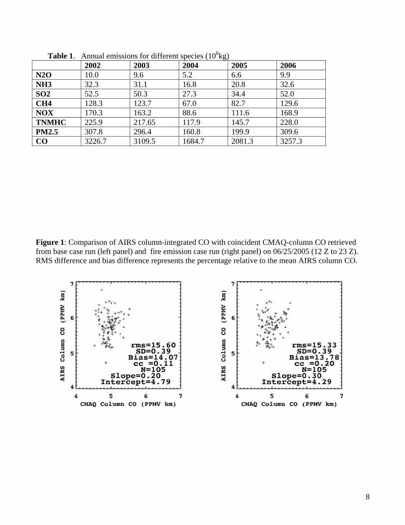
Figure 1 shows the comparison between column-integrated values of CO from AIRS and CMAQ (base case and GOES fire emission case, separately). The CMAQ CO calculated with fire emissions is more comparable with AIRS CO with smaller RMS difference. GOES fire emission inventory certainly helps to reduce the uncertainty, which is attributable to the reduction in bias (systematic difference) because random difference (standard deviation) is not improved.

This preliminary comparison only indicates that CMAQ CO estimates are improved by adding GOES fire emissions inventory. In this case, biomass burning emissions are limited relative to background CO concentration. We believe the improvements would increase greatly for the case of severe fire emissions and AIRS CO covering the full grid area. Such comparisons are currently under way.

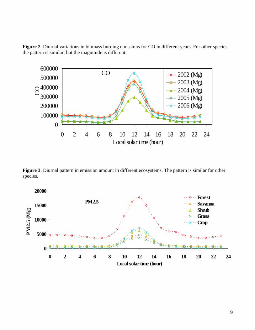
DIURNAL PATTERN OF EMISSIONS Biomass burning emissions exhibit strong diurnal patterns. The peak emission occurs around noon and large amount of emissions is released between 10:00 and 14:00 LST (Local Solar Time). It accounts for 48-66% of daily emissions during the five years although the magnitude varies greatly for different species (Figure 2). Hourly CO emissions are consistently largest, followed by PM2.5, TNMHC, NOX, CH4, SO2, NH3, and N2O. The annual average of peak value during 2002-2006 is as large as 291.0×106~546.9×106 kg/h, 28.2×106~52.5×106 kg/h, 20.4×106~38.3×106 kg/h, 16.1×106~29.3×106 kg/h, 11.6×106~21.7×106 kg/h, 5.0×106~9.0×106 kg/h, 2.9×106~5.5×106 kg/h, 0.9×106~1.7×106 kg/h, for CO, PM2.5, TNMHC, NOX, CH4, SO2, NH3, and N2O, respectively. The emission difference among these species is associated with the variations in the corresponding emission factors23. The magnitudes of hourly emissions are dependent on ecosystem types (Figure 3). Hourly emissions in forests are distinctively larger relatively to those in other ecosystems since the fuel loadings are generally largest in forest regions. It is followed by the values in shrublands because the related burned areas are always large in the semiarid environemnt21. In croplands, hourly emissions are the third largest during noon but they are minima during off peak hours. It is due to the fact that agriculture fires are strongly controlled by human activities during daytime. Peak emissions are similarly smallest in savannas and grasslands. For example, the released NOX (annual average) in peak hour is 8.8×106, 2.5×106, 4.8×106, 2.3×106, 4.0×106 kg in forests, savannas, shrublands, grasslands, and croplands, respectively. The CO emission is 192.0×106, 47.7×106, 56.1×106, 36.7×106, 71.2×106 kg, respectively.

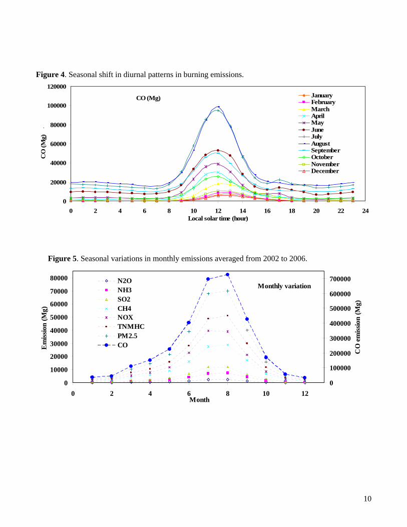
Diurnal patterns in emissions shift slightly in different seasons. The hourly emissions are large in 9:00-16:00 LST throughout the year. However, the peak hourly emission occurs around 12:00 LST from March to October, while it shifts slightly to 13:00 LST from November to next February (Figure 4). This is likely associated with seasonal variation in fire weather including humidity and temperature. SEASONAL AND INTER-ANNUAL VARIATIONS IN BIOMASS BURNING EMISSIONS

5

Biomass burning emissions present distinctive variations in monthly and annual values (Figure 5). Average monthly values between 2002 and 2006 indicate that the emissions are mainly released in July and August, which account for about 47% of annual emissions. In contrast, the emissions from November to next February only account for about 5%. The coefficient of variation in the monthly data is about 98%. Certainly, biomass burning occurs often in dry and hot summer and is limited during wet and cold winter.

Inter-annual variations in emissions are also significant. During the five years, emissions are similarly large in 2002 and 2006, which are almost doubled relative to the values in 2004 (Table 1). The mean annual emission is 8.3×106, 26.7×106, 43.3×106, 106.3×106, 140.5×106, 187.0×106, 254.9×106, and 2671.9×106 for N2O, NH3, SO2, CH4, NOX, TNMHC, PM2.5, and CO, separately. The coefficient of variation is about 27%. The inter-annual variations also differ in different ecosystems. The coefficient of variation is 35.7%, 21.7%, 33.2%, 26.6, and 31.3% for forests, savannas, shrubs, grasses, and crops, respectively. This indicates that the largest variation occurs in forests while the value is relatively small in savannas.

SPATIAL SHIFT IN EMISSIONS

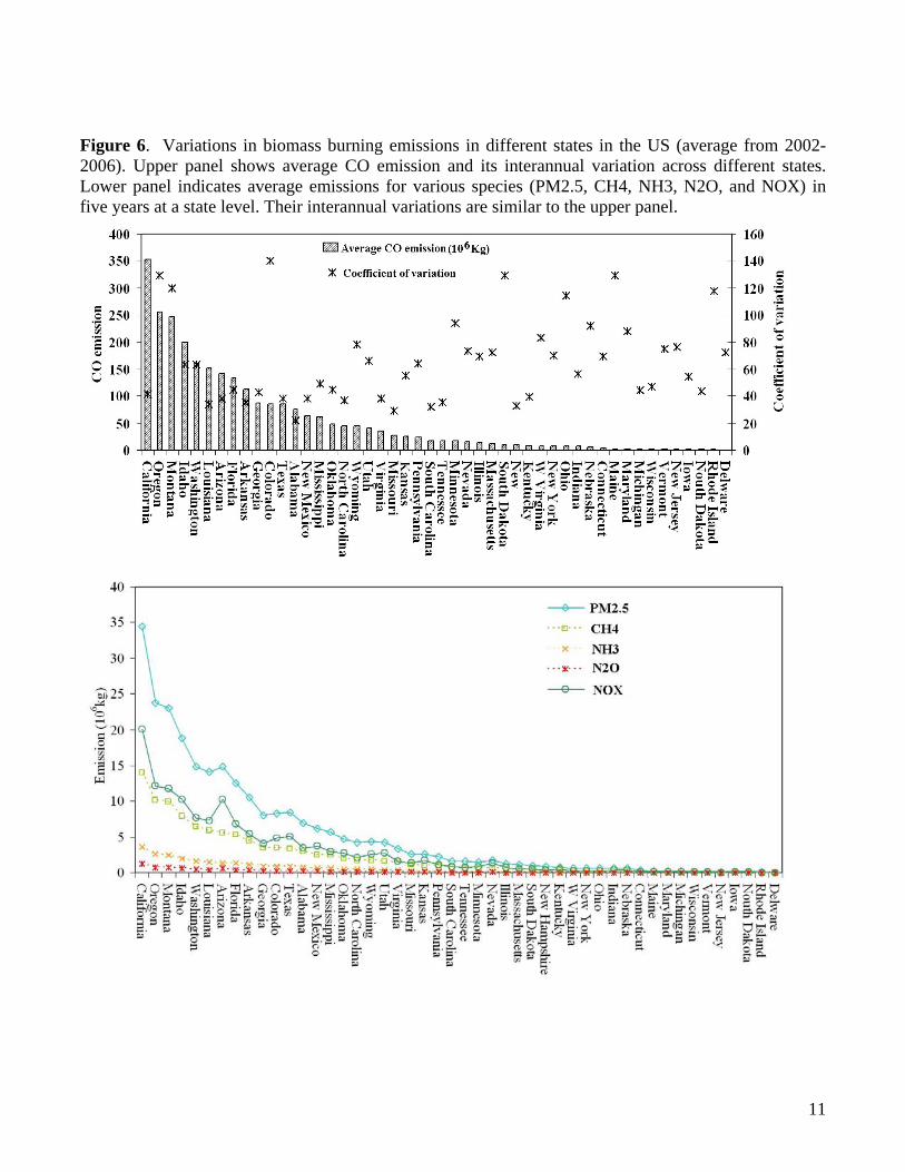
Emissions at a state level reveal distinguishable spatial patterns. Among forty eight states across CONUS, twenty states with large emissions account for 91% of the total values. Among them, eleven sates are located in western US, four sates in southern Mississippi valley, and five in southeastern US. The top five states account for more than 45% of the total emissions, which are all located in western US (Figure 6). Inter-annual variation in emissions differs greatly for different states. The coefficient of variation (CV) is larger than 50% in most of the states. Specifically, CV is larger than 120% in Oregon, Montana, and Colorado. In contrast, annual emissions are relatively stable in southern Mississippi River and southeastern CONUS, where CVis less than 50% (Figure 6), which is likely associated with relatively stable agriculture emissions.

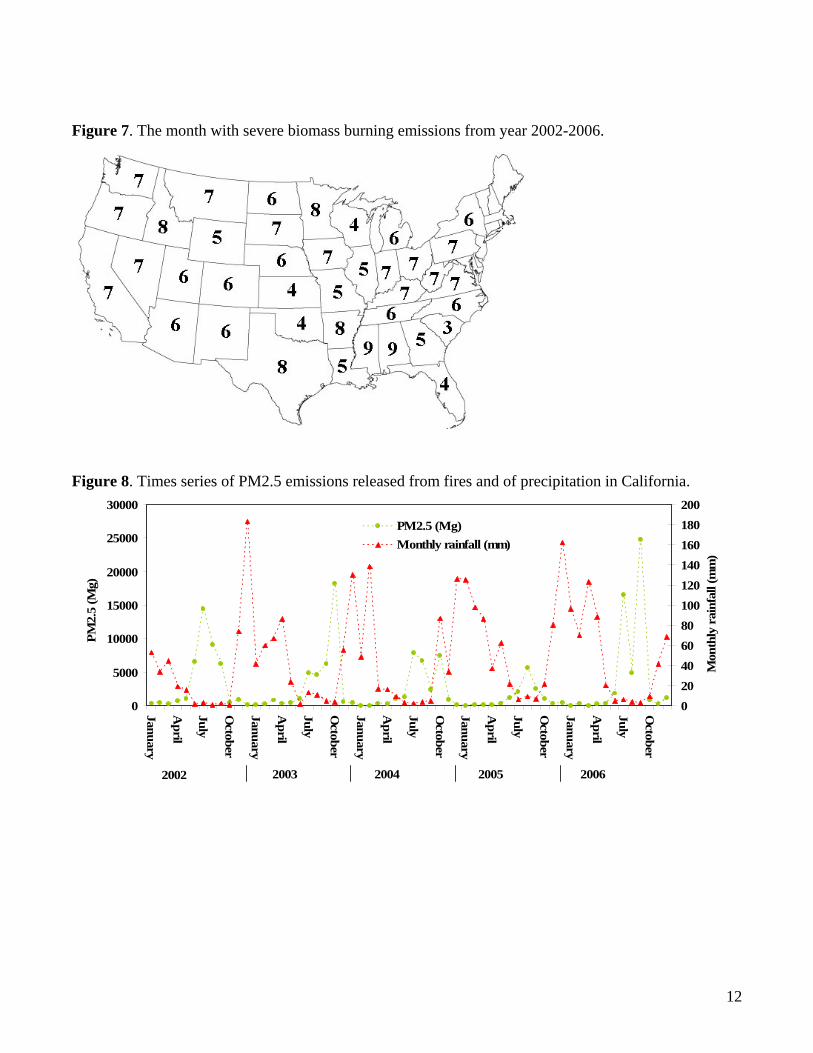
The severe monthly emissions reflect the spatial shift in seasonal emissions across CONUS (Figure 7). Biomass burning releases a large amount of trace gases and aerosols in June-September in western US such as Arizona and California, in early spring in Oklahoma and Florida (preparing for crop planting), and in later autumn (September–October) in Alabama and Mississippi (after crop harvest). The severe fire season (month) accounts for more than 40% of annual emissions. This pattern is associated with the fire climate and human activity. In agriculture areas, the severe emission pattern reflects that agricultural fires could be set during the harvesting, post-harvesting, and pre-planting periods across CONUS. It is because the agricultural burning is used for clearing crop residue, fertilizing the soil, and eliminating insects and disease from the fields26, 27. In contrast, the severe fire emissions in other ecosystems are strongly controlled by dry climate. For example, emissions in California are mainly released from wildfire, where monthly peak emission corresponds to the minimum of monthly precipitation (Figure 8). Biomass burning emissions increase exponentially with the decrease of precipitation. DISCUSSION AND CONCLUSIONS Biomass burning emissions can be estimated in near real time using multiple satellite data. The fuel loadings derived from MODIS land data provide detailed spatial variability. The GOES fire observations are essential for investigating diurnal burning behaviors. AVHRR-based moisture modifies the emission and combustion factors in different climate seasons. As a result, the algorithm used in this study provides a useful tool to monitor biomass burning emissions in near real time and to generate emission inventory across the CONUS. The evaluation of the biomass burning emissions using CMAQ CO and AIRS CO indicates adding fire emissions could improve air quality modeling although more detailed investigations are required. The emissions data during 2002-2006 indicate that biomass burning emissions present strong diurnal patterns. The large amount of emissions is released from 10:00-16:00 LST with peak around noon. This certainly affects air quality during daytime and has a strong impact on human activities.

6

Seasonal variation in biomass burning emissions is distinct. The emission amount is generally high in July and August across CONUS, but the month with severe emissions varies greatly in different states. This variation is a function of human activity (agriculture) and weather patterns. Further, the emission increases exponentially with the decrease of monthly precipitation. This relationship could be potentially used for the predication of biomass burning emissions with the change of climate. Spatial pattern in biomass burning emissions varies strongly across the CONUS. The emissions are large in west and southern east US. The top 10 states with largest fire emissions are California, Oregon, Montana, Idaho, Washington, Louisiana, Arizona, Florida, Arkansas, and Georgia. Acknowledgments. The authors wish to thank Christopher Schmidt and Elaine Prins for providing GOES WF_ABBA fire data and George Pouliot for CMAQ data. The views, opinions, and findings contained in those works are these of the author(s) and should not be interpreted as an official NOAA or US Government position, policy, or decision. REFERENCES 1Soja, A.J., Sukhinin, A.I., Cahoon, D.R., Shugart, H.H., Stackhouse, P.W. “AVHRR-derived fire frequency, distribution and area burned in Siberia,”, International Journal of Remote Sensing, 2004, 25 (10): 1939-1960 2Seiler, W. and Crutzen, P.J., “Estimates of gross and net fluxes of carbon between the biosphere and the atmosphere from biomass burning,”, Climatic Change, 1980, 2, 207-247 3Schultz, M.G., Diehl, T., Brasseur, G.P., Zittel, W. “Air pollution and climate-forcing impacts of a global hydrogen economy,”, Science, 2003, 302 (5645): 624-627. 4Phuleria, H.C., Fine, P.M., Zhu, Y.F., Sioutas, C. “Air quality impacts of the October 2003 Southern California wildfires,”, Journal Of Geophysical Research-Atmospheres, 2005,110 (D7): Art. No. D07S20. 5Sapkota, A., Symons, J.M., Kleissl, J., Wang, L., Parlange, M.B., Ondov, J., Breysse, P.N., Diette, G.B., Eggleston, P.A., Buckley, T.J. “Impact of the 2002 Canadian forest fires on particulate matter air quality in Baltimore City,”, Environmental Science & Technology, 2005, 39 (1): 24-32. 6Goode, J.G., Yokelson, R.J., Ward, D.E., Susott, R.A., Babbitt, R.E., Davies, M.A., Hao, W.M. “Measurements of excess O-3, CO2, CO, CH4, C2H4, C2H2, HCN, NO, NH3, HCOOH, CH3COOH, HCHO, and CH3OH in 1997 Alaskan biomass burning plumes by airborne fourier transform infrared spectroscopy (AFTIR),”, Journal Of Geophysical Research-Atmospheres, 2000, 105(D17): 22147-22166. 7Liu, Y. “Variability of wildland fire emissions across the contiguous United States”, Atmospheric Environment, 2004, 38: 3489–3499. 8Freitas, S.R., Longo, K.M., Diasb, M.A.F.S, Diasb, P.L.S., Chatfield, R., Prins, E., Artaxo, P., Grell, G.A., Recuero, F.S. “Monitoring the transport of biomass burning emissions in South America,”, Environmental Fluid Mechanics, 2005, 5 (1-2): 135-167. 9Wiedinmyer, C., Quayle, B., Geron, C., Belote A., McKenzie, D., Zhang, X., O’Neill, S., and Wynne, K.K., “Estimating emissions from fires in north America for air quality modeling,”, Atmospheric Environment, 2006, in press. 10Deeming, J.E., Gurgan, R.E., Cohen, J.D., The National Fire-Danger Rating System-1978. Ogden, UT: United States Department of Agriculture, Forest Service, Intermountain Forest and Range Experiment Station, General Technical Report INT-39, 1977, 66p. 11Sandberg , D.V., Ottmar, R.D., Cushon, G.H. “Characterizing fuels in the 21st Century,”, International Journal Of Wildland Fire, 2001,10 (3-4): 381-387.

7

12EPA.”Documentation for the Draft 1999 National Emissions Inventory (Version 3.0) for Criteria Air Pollutants and Ammonia (Area Sources)”. Prepared by E.H. Pechan & Asso.. Inc. Office of Air Quality Planning and Standards, 2003, Research Triangle Park, NC, USA. 13Eva, H., and Lambin, E.F. “Burnt area mapping in Central Africa using ATSR data,”, International Journal Of Remote Sensing, 1998; 19(18): 3473-3497. 14Duncan, B. N., Martin, R. V., Staudt, A. C., Yevich, R., and Logan, J. A., “Interannual and seasonal variability of biomass burning emissions constrained by satellite observations,”, J. Geophys. Res., 2003, 108 (D2): 4100, DOI: 10.1029/2002JD002378. 15Roy, D.P., Lewis, P.E., Justice, C.O. “Burned area mapping using multi-temporal moderate spatial resolution data - a bi-directional reflectance model-based expectation approach”, Remote Sensing Of Environment, 2002, 83 (1-2): 263-286, 16Prins, E. M., Feltz, J. M., Menzel W. P., and Ward, D. E. “An overview of GOES-8 diurnal fire and smoke results for SCAR-B and 1995 fire season in South America”, Journal of Geophysical Research, 1998, 103(D24), 31821–31835,. 17Reid, J. S., Prins, E. M., Westphal, D. L., Schmidt, C. C., Richardson, K. A., Christopher, S. A., Eck, T. F., Reid, E. A., Curtis, C. A., and Hoffman, J.P., “Real-time monitoring of South American smoke particle emissions and transport using a coupled remote sensing/box-model approach”, Geophysical Research Letter, 2004, 31, L06107, DOI: 10.1029/2003GL018845. 18Ito, A., Penner, J. E. “Global estimates of biomass burning emissions based on satellite imagery for the year 2000,”, Journal of Geophysical Research, 2004, 109, D14S05. 19Zhang, X., Kondragunta, S. “Estimating forest biomass in the USA using generalized allometric model and MODIS land data”, Geographical Research Letter, 2006, 33, L09402, doi:10.1029/2006GL025879. 20Zhang, X., Kondragunta, S., Schmidt, C., Kogan, F. “Near real-time monitoring of biomass burning particulate emissions (PM2.5) across the Contiguous United States using multiple satellite instruments”, Atmospheric Environment, 2008, in press. 21Zhang, X., Kondragunta, S. “Temporal and spatial variability in biomass burned areas across the USA derived from the GOES fire product”, Remote Sensing of Environment, 2008, doi:10.1016/j.rse.2008.02.006. 22Anderson, G.K., Sandberg D. V., and Norheim, R. A. “Fire Emission Production Simulator (FEPS) User’s Guide (version 1.0)”, 2004, http://www.fs.fed.us/pnw/fera/publications/fulltext/FEPS_User_Guide.pdf. 23Reinhardt E. D., Keane R. E., Brown J. K. “First Order Fire Effects Model: FOFEM 4.0, user's guide ( General . Technical. Report. INT-GTR-344)”. Ogden, UT: U.S. Department of Agriculture, Forest Service, Intermountain Research Station, 65 p. 1997. 24McMillan, W. W., C. Barnet, L. Strow, M. T. Chahine, M. L. McCourt, J. X. Warner, P. C. Novelli, S. Korontzi, E. S. Maddy and S. Datta, “Daily global maps of carbon monoxide from NASA’s Atmospheric Infrared Sounder”, Geophys. Res. Letters, 2005, 32, L11801, doi:10.1029/2004GL021821. 25Mesinger, F., et al. “North American regional reanalysis”, Bulletin of the American Meteorological Society, 2006, 87, 343-360. 26Chidumayo, E. N. “A shifting cultivation land use system under population pressure in Zambia”, Agroforestry Systems, 1987, 5, 15-25. 27Korontzi, S., McCarty, J., Loboda, T., Kumar, S., Justice, C. “Gobal distribution of agricultural fires in croplands from 3 years of Moderate Resolution Imaging Spectroradiometer (MODIS) data”, Global Biogeochemical Cycles, 2006, 20, GB2021, doi:10.1029/2005GB002529.

8

Table 1. Annual emissions for different species (106kg) 2002 2003 2004 2005 2006 N2O 10.0 9.6 5.2 6.6 9.9 NH3 32.3 31.1 16.8 20.8 32.6 SO2 52.5 50.3 27.3 34.4 52.0 CH4 128.3 123.7 67.0 82.7 129.6 NOX 170.3 163.2 88.6 111.6 168.9 TNMHC 225.9 217.65 117.9 145.7 228.0 PM2.5 307.8 296.4 160.8 199.9 309.6 CO 3226.7 3109.5 1684.7 2081.3 3257.3

Figure 1: Comparison of AIRS column-integrated CO with coincident CMAQ-column CO retrieved from base case run (left panel) and fire emission case run (right panel) on 06/25/2005 (12 Z to 23 Z). RMS difference and bias difference represents the percentage relative to the mean AIRS column CO.

9

Figure 2. Diurnal variations in biomass burning emissions for CO in different years. For other species, the pattern is similar, but the magnitude is different.

CO

0100000200000300000400000500000600000

0 2 4 6 8 10 12 14 16 18 20 22 24Local solar time (hour)

CO

2002 (Mg)2003 (Mg)2004 (Mg)2005 (Mg)2006 (Mg)

Figure 3. Diurnal pattern in emission amount in different ecosystems. The pattern is similar for other species.

PM2.5

0

5000

10000

15000

20000

0 2 4 6 8 10 12 14 16 18 20 22 24Local solar time (hour)

PM2.

5 (M

g)

ForestSavannaShrubGrassCrop

10

Figure 4. Seasonal shift in diurnal patterns in burning emissions.

CO (Mg)

0

20000

40000

60000

80000

100000

120000

0 2 4 6 8 10 12 14 16 18 20 22 24Local solar time (hour)

CO

(Mg)

-

JanuaryFebruaryMarchAprilMayJuneJulyAugustSeptemberOctoberNovemberDecember

Figure 5. Seasonal variations in monthly emissions averaged from 2002 to 2006.

Monthly variation

0

10000

20000

30000

40000

50000

60000

70000

80000

0 2 4 6 8 10 12Month

Em

issio

n (M

g)

0

100000

200000

300000

400000

500000

600000

700000

CO

em

issio

n (M

g)

N2ONH3SO2CH4NOXTNMHCPM2.5CO

11

Figure 6. Variations in biomass burning emissions in different states in the US (average from 2002-2006). Upper panel shows average CO emission and its interannual variation across different states. Lower panel indicates average emissions for various species (PM2.5, CH4, NH3, N2O, and NOX) in five years at a state level. Their interannual variations are similar to the upper panel.

12

Figure 7. The month with severe biomass burning emissions from year 2002-2006.

Figure 8. Times series of PM2.5 emissions released from fires and of precipitation in California.

0

5000

10000

15000

20000

25000

30000

January

April

July

October

January

April

July

October

January

April

July

October

January

April

July

October

January

April

July

October

PM2.

5 (M

g)

020406080100120140160180200

Mon

thly

rai

nfal

l (m

m)

PM2.5 (Mg)Monthly rainfall (mm)

2002 20052003 2004 2006