homoclinic orbits of the fitzhughâ€“nagumo equation

SIAM J. APPLIED DYNAMICAL SYSTEMS c© 2010 Society for Industrial and Applied MathematicsVol. 9, No. 1, pp. 138–153

Homoclinic Orbits of the FitzHugh–Nagumo Equation: Bifurcations in the FullSystem∗

John Guckenheimer† and Christian Kuehn‡

Abstract. This paper investigates travelling wave solutions of the FitzHugh–Nagumo equation from the view-point of fast-slow dynamical systems. These solutions are homoclinic orbits of a three dimensionalvector field depending upon system parameters of the FitzHugh–Nagumo model and the wave speed.Champneys et al. [SIAM J. Appl. Dyn. Syst., 6 (2007), pp. 663–693] observed sharp turns in thecurves of homoclinic bifurcations in a two dimensional parameter space. This paper demonstratesnumerically that these turns are located close to the intersection of two curves in the parameterspace that locate nontransversal intersections of invariant manifolds of the three dimensional vectorfield. The relevant invariant manifolds in phase space are visualized. A geometrical model inspiredby the numerical studies displays the sharp turns of the homoclinic bifurcations curves and yieldsquantitative predictions about multipulse and homoclinic orbits and periodic orbits that have notbeen resolved in the FitzHugh–Nagumo model. Further observations address the existence of canardexplosions and mixed-mode oscillations.

Key words. homoclinic bifurcation, singular perturbation, invariant manifolds

AMS subject classifications. Primary, 34E13, 34E15, 37G20, 37D10; Secondary, 34C26, 37D45

DOI. 10.1137/090758404

1. Introduction. This paper investigates the three dimensional FitzHugh–Nagumo vectorfield defined by

εx1 = x2,

εx2 =1

Δ(sx2 − x1(x1 − 1)(α − x1) + y − p) =:

1

Δ(sx2 − f(x1) + y − p) ,(1.1)

y =1

s(x1 − y) ,

where p, s, Δ, α, and ε are parameters. Our analysis views equations (1.1) as a fast-slowsystem with two fast variables and one slow variable. The dynamics of system (1.1) werestudied extensively by Champneys et al. [4] with an emphasis on homoclinic orbits thatrepresent travelling wave profiles of a partial differential equation [1]. Champneys et al. [4]used numerical continuation implemented in AUTO [6] to analyze the bifurcations of (1.1)for ε = 0.01 with varying p and s. As in their studies, we choose Δ = 5, α = 1/10 for thenumerical investigations in this paper. The main structure of the bifurcation diagram is shownin Figure 1.

∗Received by the editors May 6, 2009; accepted for publication (in revised form) by T. Kaper November 22,2009; published electronically February 5, 2010.

http://www.siam.org/journals/siads/9-1/75840.html†Mathematics Department, Cornell University, Ithaca, NY 14853 ([email protected]).‡Center for Applied Mathematics, Cornell University, Ithaca, NY 14853 ([email protected]).

138

http://www.siam.org/journals/siads/9-1/75840.html

mailto:[email protected]

mailto:[email protected]

FHN EQUATION: BIFURCATIONS IN THE FULL SYSTEM 139

−0.2 −0.1 0 0.1 0.2 0.3 0.4 0.50

0.2

0.4

0.6

0.8

1

1.2

1.4

1.6

I

p

sHom

Hopf

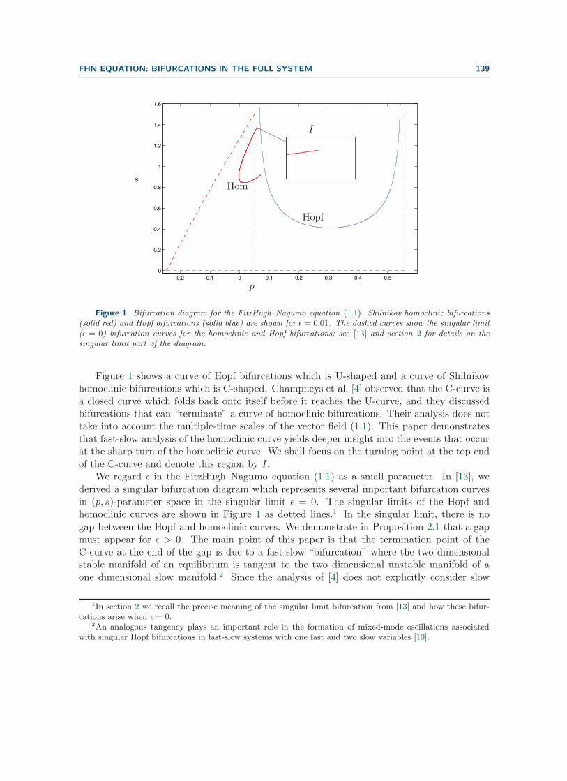
Figure 1. Bifurcation diagram for the FitzHugh–Nagumo equation (1.1). Shilnikov homoclinic bifurcations(solid red) and Hopf bifurcations (solid blue) are shown for ε = 0.01. The dashed curves show the singular limit(ε = 0) bifurcation curves for the homoclinic and Hopf bifurcations; see [13] and section 2 for details on thesingular limit part of the diagram.

Figure 1 shows a curve of Hopf bifurcations which is U-shaped and a curve of Shilnikovhomoclinic bifurcations which is C-shaped. Champneys et al. [4] observed that the C-curve isa closed curve which folds back onto itself before it reaches the U-curve, and they discussedbifurcations that can “terminate” a curve of homoclinic bifurcations. Their analysis does nottake into account the multiple-time scales of the vector field (1.1). This paper demonstratesthat fast-slow analysis of the homoclinic curve yields deeper insight into the events that occurat the sharp turn of the homoclinic curve. We shall focus on the turning point at the top endof the C-curve and denote this region by I.

We regard ε in the FitzHugh–Nagumo equation (1.1) as a small parameter. In [13], wederived a singular bifurcation diagram which represents several important bifurcation curvesin (p, s)-parameter space in the singular limit ε = 0. The singular limits of the Hopf andhomoclinic curves are shown in Figure 1 as dotted lines.1 In the singular limit, there is nogap between the Hopf and homoclinic curves. We demonstrate in Proposition 2.1 that a gapmust appear for ε > 0. The main point of this paper is that the termination point of theC-curve at the end of the gap is due to a fast-slow “bifurcation” where the two dimensionalstable manifold of an equilibrium is tangent to the two dimensional unstable manifold of aone dimensional slow manifold.2 Since the analysis of [4] does not explicitly consider slow

1In section 2 we recall the precise meaning of the singular limit bifurcation from [13] and how these bifur-cations arise when ε = 0.

2An analogous tangency plays an important role in the formation of mixed-mode oscillations associatedwith singular Hopf bifurcations in fast-slow systems with one fast and two slow variables [10].

140 JOHN GUCKENHEIMER AND CHRISTIAN KUEHN

manifolds of the system, this tangency does not appear on their list of possibilities for thetermination of a C-curve. Note that the slow manifolds of the system are unique only up to“exponentially small” quantities of the form exp(−c/ε), c > 0, so our analysis identifies onlythe termination point up to exponentially small values of the parameters.

Fast-slow dynamical systems can be written in the form

εx = εdx

dτ= f(x, y, ε),(1.2)

y =dy

dτ= g(x, y, ε),

where (x, y) ∈ Rm×R

n and ε is a small parameter 0 < ε� 1. The functions f : Rm×Rn×R →

Rm and g : Rm×R

n×R → Rn are analytic in the systems studied in this paper. The variables

x are fast and the variables y are slow. We can change (1.2) from the slow time scale τ to thefast time scale t = τ/ε, yielding

x′ =dx

dt= f(x, y, ε),(1.3)

y′ =dy

dt= εg(x, y, ε).

In the singular limit ε → 0 the system (1.2) becomes a differential-algebraic equation. Thealgebraic constraint defines the critical manifold:

C0 = {(x, y) ∈ Rm × R

n : f(x, y, 0) = 0}.

For a point p ∈ C0 we say that C0 is normally hyperbolic at p if all the eigenvalues of them × m matrix Dxf(p) have nonzero real parts. A normally hyperbolic subset of C0 is anactual manifold, and we can locally parametrize it by a function h(y) = x. This yields theslow subsystem (or reduced flow) y = g(h(y), y) defined on C0. Taking the singular limit ε → 0in (1.3) gives the fast subsystem (or layer equations) x′ = f(x, y) with the slow variables yacting as parameters. Fenichel’s theorem [8] states that normally hyperbolic critical manifoldsperturb to invariant slow manifolds Cε. A slow manifold Cε is O(ε) distance away from C0.The flow on the (locally) invariant manifold Cε converges to the slow subsystem on the criticalmanifold as ε → 0. Slow manifolds are usually not unique for a fixed value of ε = ε0 but lieat a distance O(e−K/ε0) away from each other for some K > 0; nevertheless we shall refer to“the slow manifold” for a fast-slow system with the possibility of an exponentially small errorbeing understood.

Section 2 discusses the fast-slow decomposition of the homoclinic orbits of the FitzHugh–Nagumo equation in the region I. This decomposition has been used to prove the existenceof homoclinic orbits in the system for ε sufficiently small [2, 15, 19, 18, 22], but previous workapplies only to a situation where the equilibrium point for the homoclinic orbit is not closeto a fold point. At a fold point the critical manifold of a fast-slow system is locally quadraticand not normally hyperbolic. This new aspect of the decomposition is key to understandingthe sharp turn of the homoclinic curve. Section 3 presents a numerical study that highlightsthe geometric mechanism for the turning of the C-curve. We visualize relevant aspects of


the phase portraits near the turns of the C-curve. In section 4 we show that exponentialcontraction of the Shilnikov return map in the FitzHugh–Nagumo equation explains why n-homoclinic and n-periodic orbits are expected to be found at parameter values very close toa primary 1-homoclinic orbit. Section 5 presents two further observations. We identify wherea canard explosion [23] occurs and note the existence of two different types of mixed-modeoscillations in the system.

2. Fast-slow decomposition of homoclinic orbits. We introduce notation used in ourearlier work [13]. The critical manifold of (1.1) is given by

C0 = {(x1, x2, y) ∈ R3 : x2 = 0 and y = f(x1) + p}.

It is normally hyperbolic away from the two fold points x1,±, with x1,− < x1,+, which arefound by solving f ′(x1) = 0 as the local minimum and maximum of the cubic f . Hence C0

splits into three parts:

Cl = {x1 < x1,−} ∩ C0, Cm = {x1,− ≤ x1 ≤ x1,+} ∩ C0, Cr = {x1,+} ∩ C0.

We are mostly interested in the two branches Cl and Cr which are of saddle type; i.e., points inCl and Cr are saddle equilibria of the fast subsystem. The middle branch Cm−{x1,±} consistsof unstable foci for the fast subsystem. The slow manifolds provided by Fenichel’s theoremwill be denoted by Cl,ε and Cr,ε. The notation for the two dimensional stable and unstablemanifolds of Cl,ε is W

s(Cl,ε) and Wu(Cr,ε) with similar notation for Cr,ε; the notation for the

associated linear eigenspaces is, e.g., Es(Cl,ε). The full system (1.1) has a unique equilibriumpoint which we denote by q. For (p, s) ∈ I and ε = 0.01 the dimensions of the stable andunstable manifolds are dim(W u(q)) = 1 and dim(W s(q)) = 2 with a complex conjugate pairof eigenvalues for the linearization at q. The equilibrium q is completely unstable inside theU-curve, and the Hopf bifurcations we are interested in near I are all subcritical [13, 4].

As ε → 0, the Hopf bifurcation curve converges to a region in (p, s)-parameter spacebounded by two vertical lines p = p± and the segment {s = 0, p− ≤ p ≤ p+}; see Figure 1.The parameter values p± are precisely the values when the equilibrium point q coincides withthe fold points x1,± [13]. This analysis gives one part of the singular limit bifurcation diagramshowing what happens to the Hopf bifurcation curves for ε = 0.

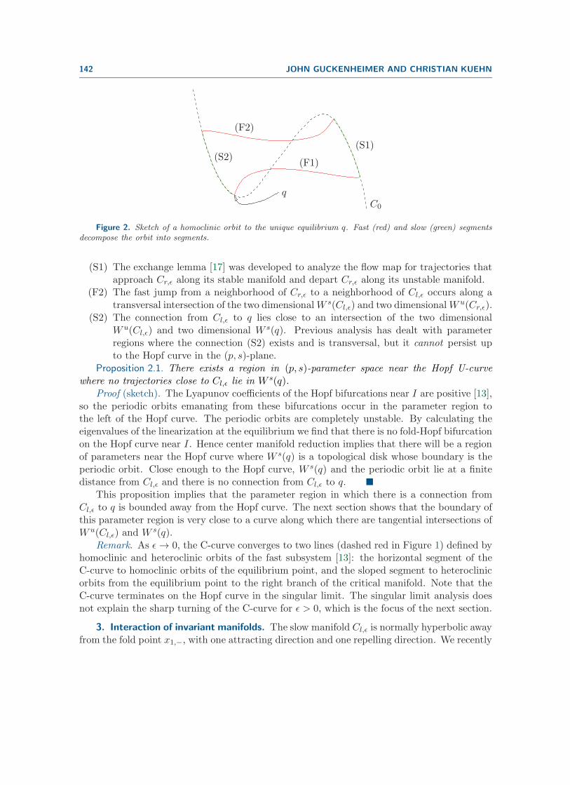
When ε is small, the homoclinic orbit in W u(q) ∩W s(q) can be partitioned into fast andslow segments. The singular limit of this fast-slow decomposition has four segments: a fastsubsystem heteroclinic connection from q to Cr, a slow segment on Cr, a heteroclinic con-nection from Cr to Cl, and a slow segment back to q on Cl; see Figure 2. Existence proofsfor the homoclinic orbits [18, 15, 2] are based upon analysis of the transitions between thesesegments. Trajectories that remain close to a normally hyperbolic slow manifold must be “ex-ponentially close” to the manifold except for short segments where the trajectory approachesthe slow manifold along its stable manifold and departs along its unstable manifold. Existenceof the homoclinic orbit depends upon how the four segments of its fast-slow decomposition fittogether:(F1) The one dimensional W u(q) approaches Cr along its two dimensional stable manifold

W s(Cr,ε). Intersection of these manifolds cannot be transverse and occurs only forparameter values that lie along a curve in the (p, s)-parameter plane.


(F1)

(S1)

(F2)

(S2)

C0

q

Figure 2. Sketch of a homoclinic orbit to the unique equilibrium q. Fast (red) and slow (green) segmentsdecompose the orbit into segments.

(S1) The exchange lemma [17] was developed to analyze the flow map for trajectories thatapproach Cr,ε along its stable manifold and depart Cr,ε along its unstable manifold.

(F2) The fast jump from a neighborhood of Cr,ε to a neighborhood of Cl,ε occurs along atransversal intersection of the two dimensionalW s(Cl,ε) and two dimensionalW u(Cr,ε).

(S2) The connection from Cl,ε to q lies close to an intersection of the two dimensionalW u(Cl,ε) and two dimensional W s(q). Previous analysis has dealt with parameterregions where the connection (S2) exists and is transversal, but it cannot persist upto the Hopf curve in the (p, s)-plane.

Proposition 2.1. There exists a region in (p, s)-parameter space near the Hopf U-curvewhere no trajectories close to Cl,ε lie in W s(q).

Proof (sketch). The Lyapunov coefficients of the Hopf bifurcations near I are positive [13],so the periodic orbits emanating from these bifurcations occur in the parameter region tothe left of the Hopf curve. The periodic orbits are completely unstable. By calculating theeigenvalues of the linearization at the equilibrium we find that there is no fold-Hopf bifurcationon the Hopf curve near I. Hence center manifold reduction implies that there will be a regionof parameters near the Hopf curve where W s(q) is a topological disk whose boundary is theperiodic orbit. Close enough to the Hopf curve, W s(q) and the periodic orbit lie at a finitedistance from Cl,ε and there is no connection from Cl,ε to q.

This proposition implies that the parameter region in which there is a connection fromCl,ε to q is bounded away from the Hopf curve. The next section shows that the boundary ofthis parameter region is very close to a curve along which there are tangential intersections ofW u(Cl,ε) and W

s(q).Remark. As ε→ 0, the C-curve converges to two lines (dashed red in Figure 1) defined by

homoclinic and heteroclinic orbits of the fast subsystem [13]: the horizontal segment of theC-curve to homoclinic orbits of the equilibrium point, and the sloped segment to heteroclinicorbits from the equilibrium point to the right branch of the critical manifold. Note that theC-curve terminates on the Hopf curve in the singular limit. The singular limit analysis doesnot explain the sharp turning of the C-curve for ε > 0, which is the focus of the next section.

3. Interaction of invariant manifolds. The slow manifold Cl,ε is normally hyperbolic awayfrom the fold point x1,−, with one attracting direction and one repelling direction. We recently


introduced a method [12] for computing slow manifolds of saddle type. This algorithm is usedhere to help determine whether there are connecting orbits from a neighborhood of Cl,ε to theequilibrium point q. Our numerical strategy for finding connecting orbits has three steps:

1. Choose the cross section

Σ0.09 = {(x1, x2, y) ∈ R3 : y = 0.09}

transverse to Cl,ε,2. Compute intersections of trajectories in W s(q) with Σ0.09. These points are found

either by backward integration from initial conditions that lie in a small disk D con-taining q in W s(q) or by solving a boundary value problem for trajectories that haveone end in Σ0.09 and one end on the boundary of D.

3. Compute the intersection pl ∈ Cl,ε ∩ Σ0.09 with the algorithm described in Gucken-heimer and Kuehn [12], and determine the directions of the positive and negativeeigenvectors of the Jacobian of the fast subsystem at pl.

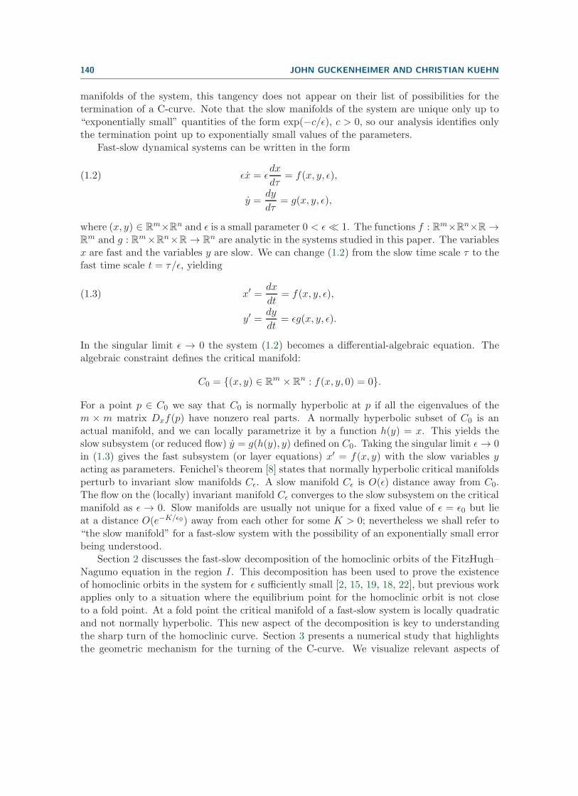
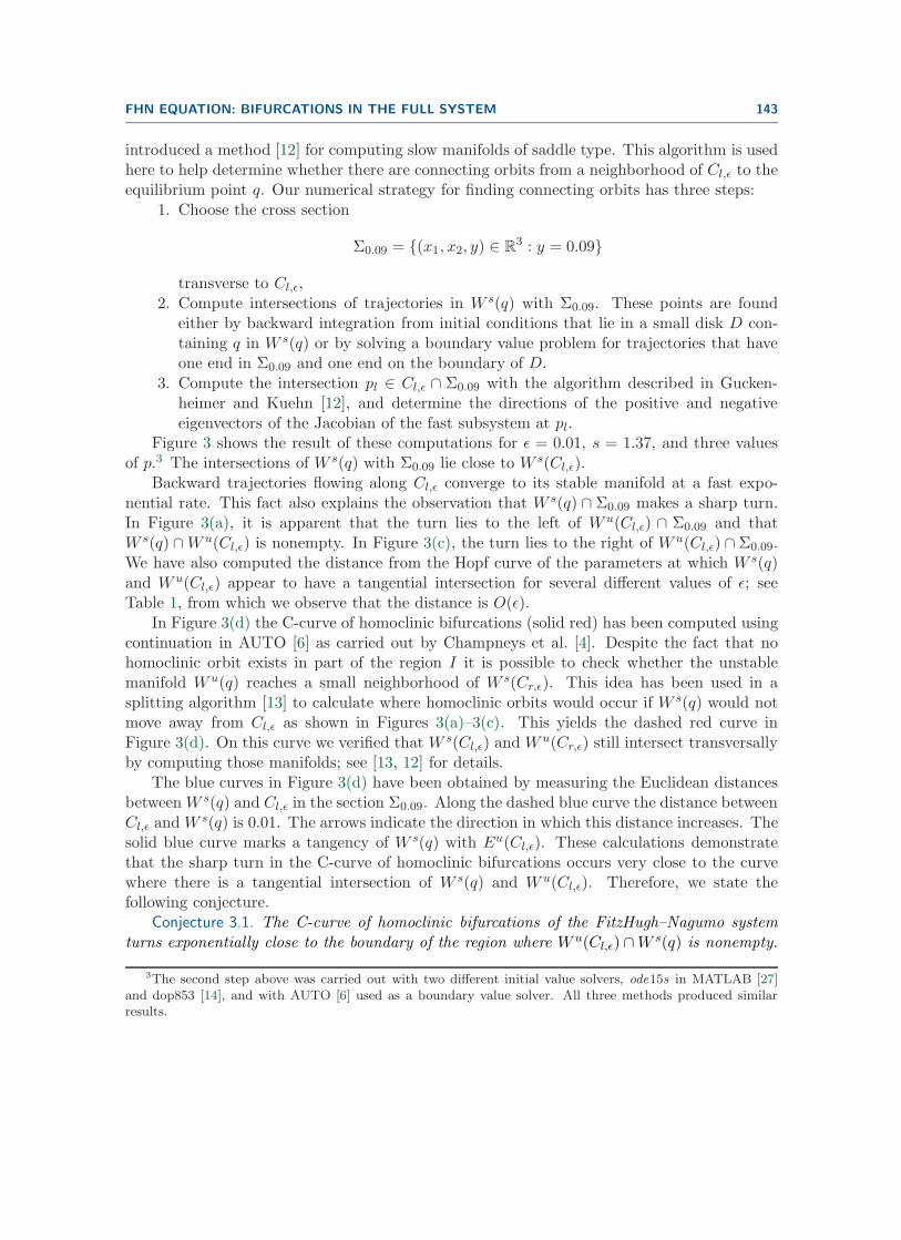
Figure 3 shows the result of these computations for ε = 0.01, s = 1.37, and three valuesof p.3 The intersections of W s(q) with Σ0.09 lie close to W s(Cl,ε).

Backward trajectories flowing along Cl,ε converge to its stable manifold at a fast expo-nential rate. This fact also explains the observation that W s(q) ∩ Σ0.09 makes a sharp turn.In Figure 3(a), it is apparent that the turn lies to the left of W u(Cl,ε) ∩ Σ0.09 and thatW s(q) ∩W u(Cl,ε) is nonempty. In Figure 3(c), the turn lies to the right of W u(Cl,ε) ∩ Σ0.09.We have also computed the distance from the Hopf curve of the parameters at which W s(q)and W u(Cl,ε) appear to have a tangential intersection for several different values of ε; seeTable 1, from which we observe that the distance is O(ε).

In Figure 3(d) the C-curve of homoclinic bifurcations (solid red) has been computed usingcontinuation in AUTO [6] as carried out by Champneys et al. [4]. Despite the fact that nohomoclinic orbit exists in part of the region I it is possible to check whether the unstablemanifold W u(q) reaches a small neighborhood of W s(Cr,ε). This idea has been used in asplitting algorithm [13] to calculate where homoclinic orbits would occur if W s(q) would notmove away from Cl,ε as shown in Figures 3(a)–3(c). This yields the dashed red curve inFigure 3(d). On this curve we verified that W s(Cl,ε) and W

u(Cr,ε) still intersect transversallyby computing those manifolds; see [13, 12] for details.

The blue curves in Figure 3(d) have been obtained by measuring the Euclidean distancesbetweenW s(q) and Cl,ε in the section Σ0.09. Along the dashed blue curve the distance betweenCl,ε andW

s(q) is 0.01. The arrows indicate the direction in which this distance increases. Thesolid blue curve marks a tangency of W s(q) with Eu(Cl,ε). These calculations demonstratethat the sharp turn in the C-curve of homoclinic bifurcations occurs very close to the curvewhere there is a tangential intersection of W s(q) and W u(Cl,ε). Therefore, we state thefollowing conjecture.

Conjecture 3.1. The C-curve of homoclinic bifurcations of the FitzHugh–Nagumo systemturns exponentially close to the boundary of the region where W u(Cl,ε) ∩W s(q) is nonempty.

3The second step above was carried out with two different initial value solvers, ode15s in MATLAB [27]and dop853 [14], and with AUTO [6] used as a boundary value solver. All three methods produced similarresults.


−0.25 −0.2 −0.15 −0.1 −0.05 0 0.05 0.1−0.03

−0.02

−0.01

0

0.01

0.02

0.03

0.04

x1

x2

W s(q)W s(Cl,ε)

W u(Cl,ε)

(a) p = 0.059, s = 1.37

−0.25 −0.2 −0.15 −0.1 −0.05 0 0.05 0.1−0.03

−0.02

−0.01

0

0.01

0.02

0.03

0.04

x1

x2

W s(q)W s(Cl,ε)

W u(Cl,ε)

(b) p = 0.0595, s = 1.37

−0.25 −0.2 −0.15 −0.1 −0.05 0 0.05 0.1−0.04

−0.02

0

0.02

0.04

0.06

x1

x2W s(q)

W s(Cl,ε)

W u(Cl,ε)

(c) p = 0.06, s = 1.37

0.059 0.0592 0.0594 0.0596 0.0598 0.061.365

1.37

1.375

1.38

1.385

1.39

p

s

(d) Parameter space, region I .

Figure 3. Figures (a)–(c) show the movement of the stable manifold W s(q) (cyan) with respect to Eu(Cl,ε)(red) and Es(Cl,ε) (green) in phase space on the section y = 0.09 for ε = 0.01. The parameter space diagram (d)shows the homoclinic C-curve (solid red), an extension of the C-curve of parameters where W u(q) ∩W s(Cr,ε)is nonempty, a curve that marks the tangency of W s(q) to Eu(Cl,ε) (blue), and a curve that marks a distancebetween Cl,ε and W s(q) (dashed blue) of 0.01 where the arrows indicate the direction in which the distance isbigger than 0.01. The solid black squares in (d) show the parameter values for (a)–(c).

Table 1Euclidean distance in (p,s)-parameter space between the Hopf curve and the location of the tangency point

between W s(q) and W u(Cl,ε).

ε D = d (tangency, Hopf)

10−2 ≈ 1.07ε10−3 ≈ 1.00ε10−4 ≈ 0.98ε

Note that trajectory segments of types (F1), (S1), and (F2) are still present along thedashed red curve in Figure 3(d). Only the last slow connection (S2) no longer exists. Existenceproofs for homoclinic orbits that use Fenichel’s theorem for Cl to conclude that trajectoriesentering a small neighborhood of Cl,ε must intersect W s(q) break down in this region. Theequilibrium q has already moved past the fold point x1,− in I as seen from the singularbifurcation diagram in Figure 1, where the blue dashed vertical lines mark the parametervalues where q passes through x1,±. Therefore Fenichel’s theorem does not provide the requiredperturbation of Cl,ε. Previous proofs [18, 15, 2] assumed p = 0, and the connecting orbits of


type (S2) do exist in this case.Shilnikov proved that there are chaotic invariant sets in the neighborhood of homoclinic

orbits to a saddle focus in three dimensional vector fields when the magnitude of the real eigen-value is larger than the magnitude of the real part of the complex pair of eigenvalues [28]. Thehomoclinic orbits of the FitzHugh–Nagumo vector field satisfy this condition in the parameterregion I. Therefore, we expect to find many periodic orbits close to the homoclinic orbits andparameters in I with “multipulse” homoclinic orbits that have several jumps connecting theleft and right branches of the slow manifold [7]. Without making use of concepts from fast-slow systems, Champneys et al. [4] described interactions of homoclinic and periodic orbitsthat can serve to terminate curves of homoclinic bifurcations. This provides an alternate per-spective on identifying phenomena that occur near the sharp turn of the C-curve in I. AUTOcan be used to locate families of periodic orbits that come close to a homoclinic orbit as theirperiods grow.

C0

x1

x2

y

Cr,ε

W s(Cl,ε)

Cl,ε

W s(q)

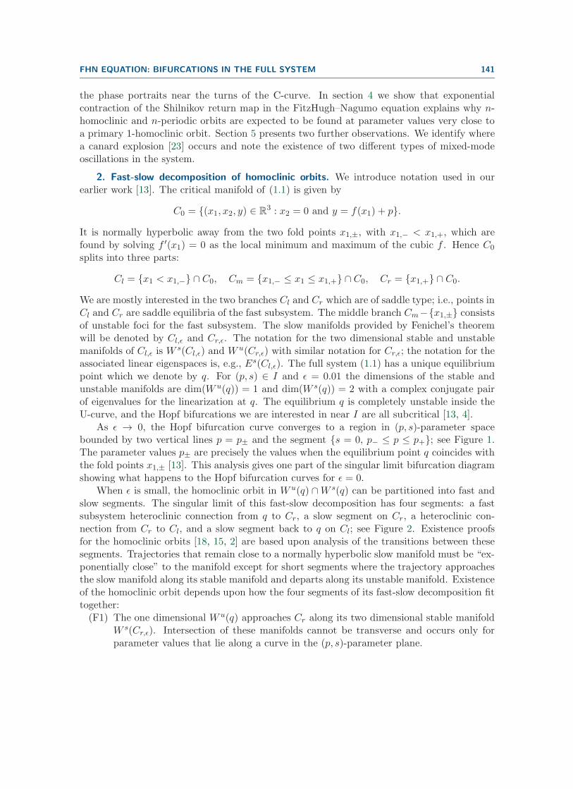
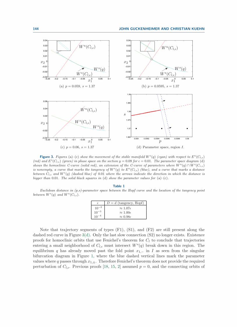
Figure 4. Phase space along the C-curve near its sharp turn: the parameter values ε = 0.01, p = 0.05,and s ≈ 1.3254 lie on the C-curve. The homoclinic orbit (red), two periodic orbits born in the subcritical Hopfbifurcation (blue), C0 (thin black), and Cl,ε and Cr,ε (thick black) are shown. The manifold W s(q) (cyan)has been truncated at a fixed coordinate of y. Furthermore, W s(Cl,ε) (green) is separated by Cl,ε into twocomponents shown here by dark green trajectories interacting with Cm,ε and by light green trajectories that flowleft from Cl,ε.

Figure 4 shows several significant objects in phase space for parameters lying on the C-curve. The homoclinic orbit and the two periodic orbits were calculated using AUTO. Theperiodic orbits were continued in p starting from a Hopf bifurcation for fixed s ≈ 1.3254. Notethat the periodic orbit undergoes several fold bifurcations [4]. We show two of the periodicorbits arising at p = 0.05; see [4]. The trajectories in W s(Cl,ε) have been calculated using amesh on Cl,ε and using backward integration at each mesh point and initial conditions in the


C0

x1x2

y

Cr,εCl,ε

W s(Cl,ε)

(a) Sample phase space plot between the end of the C-curve and the U-curve.

P1

P2

γ

(b) Zoom for (a) near q.

−2000 −1000

0.06

0.08

yP1

γ

T

(c) Time series.

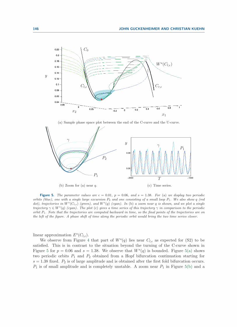
Figure 5. The parameter values are ε = 0.01, p = 0.06, and s = 1.38. For (a) we display two periodicorbits (blue), one with a single large excursion P2 and one consisting of a small loop P1. We also show q (reddot), trajectories in W s(Cl,ε) (green), and W s(q) (cyan). In (b) a zoom near q is shown, and we plot a singletrajectory γ ∈ W s(q) (cyan). The plot (c) gives a time series of this trajectory γ in comparison to the periodicorbit P1. Note that the trajectories are computed backward in time, so the final points of the trajectories are onthe left of the figure. A phase shift of time along the periodic orbit would bring the two time series closer.

linear approximation Es(Cl,ε).We observe from Figure 4 that part of W s(q) lies near Cl,ε as expected for (S2) to be

satisfied. This is in contrast to the situation beyond the turning of the C-curve shown inFigure 5 for p = 0.06 and s = 1.38. We observe that W s(q) is bounded. Figure 5(a) showstwo periodic orbits P1 and P2 obtained from a Hopf bifurcation continuation starting fors = 1.38 fixed. P2 is of large amplitude and is obtained after the first fold bifurcation occurs.P1 is of small amplitude and is completely unstable. A zoom near P1 in Figure 5(b) and a


time series comparison of a trajectory in W s(q) and P1 in Figure 5(c) show that

(3.1) limα{p : p ∈W s(q) and p �= q} = P1,

where limα U denotes the α-limit set of some set U ⊂ Rm × R

n. From (3.1) we can alsoconclude that there is no heteroclinic connection from q to P1 and only a connection from P1

to q in a large part of the region I beyond the turning of the C-curve. Since P1 is completelyunstable, there can be no heteroclinic connections from q to P1. Therefore, double heteroclinicconnections between a periodic orbit and q are restricted to periodic orbits that lie closer tothe homoclinic orbit than P1. These can be expected to exist for parameter values near theend of the C-curve in accord with the conjecture of Champneys et al. [4] and the “Shilnikov”model presented in the next section.

Remark. The recent manuscript [3] extends the results of [4] that motivated this paper.A partial unfolding of a heteroclinic cycle between a hyperbolic equilibrium point and ahyperbolic periodic orbit is developed in [3]. Champneys et al. [3] call this codimension twobifurcation an EP1t-cycle and the point where it occurs in a two dimensional parameter spacean EP1t-point. The manuscript [3] does not conclude whether the EP1t-scenario occurs inthe FitzHugh–Nagumo equation. The relationship between the results of this paper and thoseof [3] have not yet been clarified.

4. Homoclinic bifurcations in fast-slow systems. It is evident from Figure 3 that thehomoclinic orbits in the FitzHugh–Nagumo equation exist in a very thin region in (p, s)-parameter space along the C-curve. We develop a geometric model for homoclinic orbitsthat resemble those in the FitzHugh–Nagumo equation containing segments of types (S1),(F1), (S2), and (F2). The model will be seen to be an exponentially distorted version of theShilnikov model for a homoclinic orbit to a saddle focus [11]. Throughout this section weassume that the parameters lie in a region I, the region of the (p, s)-plane close to the upperturn of the C-curve.

The return map of the Shilnikov model is constructed from two components: the flow mappast an equilibrium point, approximated by the flow map of a linear vector field, composedwith a regular map that gives a “global return” of the unstable manifold of the equilibrium toits stable manifold [11]. Place two cross sections Σ1 and Σ2 moderately close to the equilibriumpoint, and model the flow map from Σ1 to Σ2 via the linearization of the vector field at theequilibrium.

The degree one coefficient of the characteristic polynomial at the equilibrium has orderO(ε), so the imaginary eigenvalues at the Hopf bifurcation point have magnitude O(ε1/2).The real part of these eigenvalues scales linearly with the distance from the Hopf curve.Furthermore, we note that the real eigenvalue of the equilibrium point remains bounded awayfrom 0 as ε→ 0.

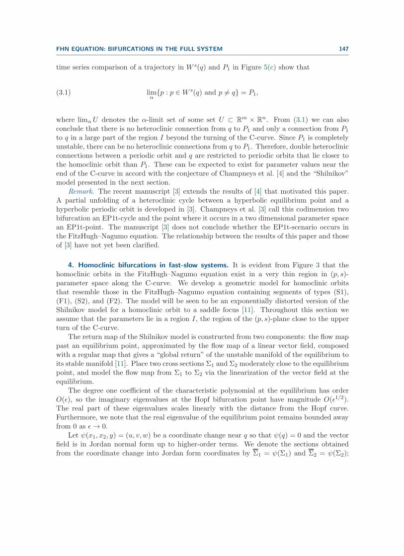
Let ψ(x1, x2, y) = (u, v, w) be a coordinate change near q so that ψ(q) = 0 and the vectorfield is in Jordan normal form up to higher-order terms. We denote the sections obtainedfrom the coordinate change into Jordan form coordinates by Σ1 = ψ(Σ1) and Σ2 = ψ(Σ2);


C0

x1x2

y

u

v

w0

F12

F21

R

Σ1

Σ2

ψ

Figure 6. Sketch of the geometric model for the homoclinic bifurcations. Only parts of the sections Σi fori = 1, 2 are shown.

see Figure 6. Then the vector field is

u′ = −βu− αv,

v′ = αu− βv + h.o.t.,(4.1)

w′ = γ,

with α, β, γ positive. We can choose ψ so that the cross sections are Σ1 = {u = 0, w > 0}and Σ2 = {w = 1}. The flow map F12 : Σ1 → Σ2 of the (linear) vector field (4.1) withouthigher-order terms is given by

(4.2) F12(v,w) = vwβ/γ

(cos

(−αγln(w)

), sin

(−αγln(w)

)).

Here β and α tend to 0 as ε → 0. The domain for F12 is restricted to the interval v ∈[exp(−2πβ/α), 1] bounded by two successive intersections of a trajectory in W s(0) with thecross section u = 0.

The global return map R : Σ2 → Σ1 of the FitzHugh–Nagumo system is obtained byfollowing trajectories that have successive segments that are near W s(Cr,ε) (fast), Cr,ε (slow),W u(Cr,ε)∩W s(Cl,ε) (fast), Cl,ε (slow), and W

u(Cl,ε) (fast). The exchange lemma [17] impliesthat the size of the domain of R in Σ2 is a strip whose width is exponentially small. As theparameter p is varied, we found numerically that the image of R has a point of quadratictangency with W s(q) at a particular value of p. We also noted that W u(q) crosses W s(Cr,ε)as the parameter s varies [13]. Thus, we choose to model R by the map

(4.3) (w, v) = F21(u, v) = (σv + λ2 − ρ2(u− λ1)2, ρ(u− λ1) + λ3)

for F21, where λ1 represents the distance of W u(q)∩Σ2 from the domain of F21, λ2 representshow far the image of F21 extends in the direction normal to W s(q), λ3 is the v coordinate ofF21(λ1, 0), and ρ

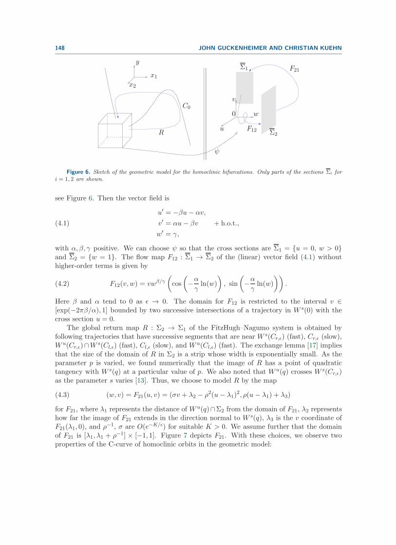
−1, σ are O(e−K/ε) for suitable K > 0. We assume further that the domainof F21 is [λ1, λ1 + ρ−1] × [−1, 1]. Figure 7 depicts F21. With these choices, we observe twoproperties of the C-curve of homoclinic orbits in the geometric model:


u

v

v

w

F21

Σ2 Σ1

W s(q)

W u(q)λ1

(λ2, λ3)

Figure 7. Sketch of the map F21 : Σ2 → Σ1. The (u, v) coordinates are centered at W u(q), and the domainof F21 is in the thin rectangle at distance λ1 from the origin. The image of this rectangle is the parabolic stripin Σ1.

1. If σv + λ2 − ρ2(u − λ1)2 is negative on the domain of F21, then the image of F21 is

disjoint from the domain of F12 and there are no recurrent orbits passing near thesaddle point. Thus, recurrence implies that λ2 > −σ.

2. If λ2 > 0, then there are two values of λ1 for which the saddle point has a single pulsehomoclinic orbit. These points occur for values of λ1 for which the w-componentof F21(0, 0) vanishes: λ1 = ±ρ−1|λ2|1/2. The magnitude of these values of λ2 isexponentially small.

When a vector field has a single pulse homoclinic orbit to a saddle focus whose real eigen-value has larger magnitude than the real part of the complex eigenvalues, Shilnikov [28] provedthat a neighborhood of this homoclinic orbit contains chaotic invariant sets. This conclusionapplies to our geometric model when it has a single pulse homoclinic orbit. Consequently,there will be a plethora of bifurcations that occur in the parameter interval λ2 ∈ [0, σ], creatingthe invariant sets as λ2 decreases from σ to 0.

The numerical results in the previous section suggest that in the FitzHugh–Nagumo systemsome of the periodic orbits in the invariant sets near the homoclinic orbit can be continued tothe Hopf bifurcation of the equilibrium point. Note that saddle-node bifurcations that createperiodic orbits in the invariant sets of the geometric model lie exponentially close to the curveλ2 = 0 that models the tangency of W s(q) and W u(Cl,ε) in the FitzHugh–Nagumo model.This observation explains why the rightmost curve of saddle-node bifurcations in Figure 7 ofChampneys et al. [4] lies close to the sharp turn of the C-curve.

There will also be curves of heteroclinic orbits between the equilibrium point and periodicorbits close to the C-curve. At least some of these form codimension two EP1t-bifurcationsnear the turn of the C-curve as discussed by Champneys et al. [4]. Thus, the tangencybetween W s(q) and W u(Cl,ε) implies that there are several types of bifurcation curves thatpass exponentially close to the sharp turn of the C-curve in the FitzHugh–Nagumo model.Numerically, any of these can be used to approximately locate the sharp turn of the C-curve.

5. Canards and mixed-mode oscillations. This section reports two additional observa-tions about the FitzHugh–Nagumo model resulting from our numerical investigations andanalysis of the turning of the C-curve.


5.1. Canard explosion. The previous sections draw attention to the intersections ofW s(q)andW u(Cl,ε) as a necessary component for the existence of homoclinic orbits in the FitzHugh–Nagumo system. Canards for the backward flow of this system occur along intersections ofW u(Cl,ε) and Cm,ε. These intersections form where trajectories that track Cl,ε have continua-tions that lie along Cm,ε, which has two unstable fast directions. We observed from Figures 4and 5 that a completely unstable periodic orbit born in the Hopf bifurcation on the U-curveundergoes a canard explosion, increasing its amplitude to the size of a relaxation oscillationorbit upon decreasing p. This canard explosion happens very close to the intersections ofW u(Cl,ε) and Cm,ε.

0.058 0.0585 0.059 0.0595 0.061.365

1.37

1.375

1.38

1.385

1.39

p

s

Hom

(a) (p, s)-space: Black circles correspond to two portraits in (b). (b) (x1, y)-projection.

Figure 8. The dashed green curve indicates where canard orbits start to occur along Cm,ε. For values ofp to the left of the dashed green curve we observe that orbits near the middle branch escape in backward time(upper panel in (b)). For values of p to the right of the dotted green curve trajectories near Cm,ε stay boundedin backward time.

To understand where this transition starts and ends we computed the middle branch Cm,ε

of the slow manifold by integrating backwards from points between the fold points x1,− andx1,+ starting close to Cm,0 and determined which side of W u(Cl,ε) these trajectories camefrom. The results are shown in Figure 8. The dashed green curve divides the (p, s)-plane intoregions where the trajectory that flows into Cm,ε lies to the left of W u(Cl,ε) and is unboundedfrom the region where the trajectory that flows into Cm,ε lies to the right of W u(Cl,ε) andcomes from the periodic orbit or another bounded invariant set. This boundary was foundby computing trajectories starting on Cm,0 backward in time. In backward time the middlebranch of the slow manifold is attracting, so the trajectory first approaches Cm,ε and thencontinues beyond its end when x1 decreases below x1,−. Figure 8(b) illustrates the differencein the behavior of these trajectories on the two sides of the dashed green curve. Figure 8shows that the parameters with canard orbits for the backward flow have smaller values ofp than those for which W s(q) and W u(Cl,ε) have a tangential intersection. The turns of theC-curve do not occur at parameters where the backward flow has canards.


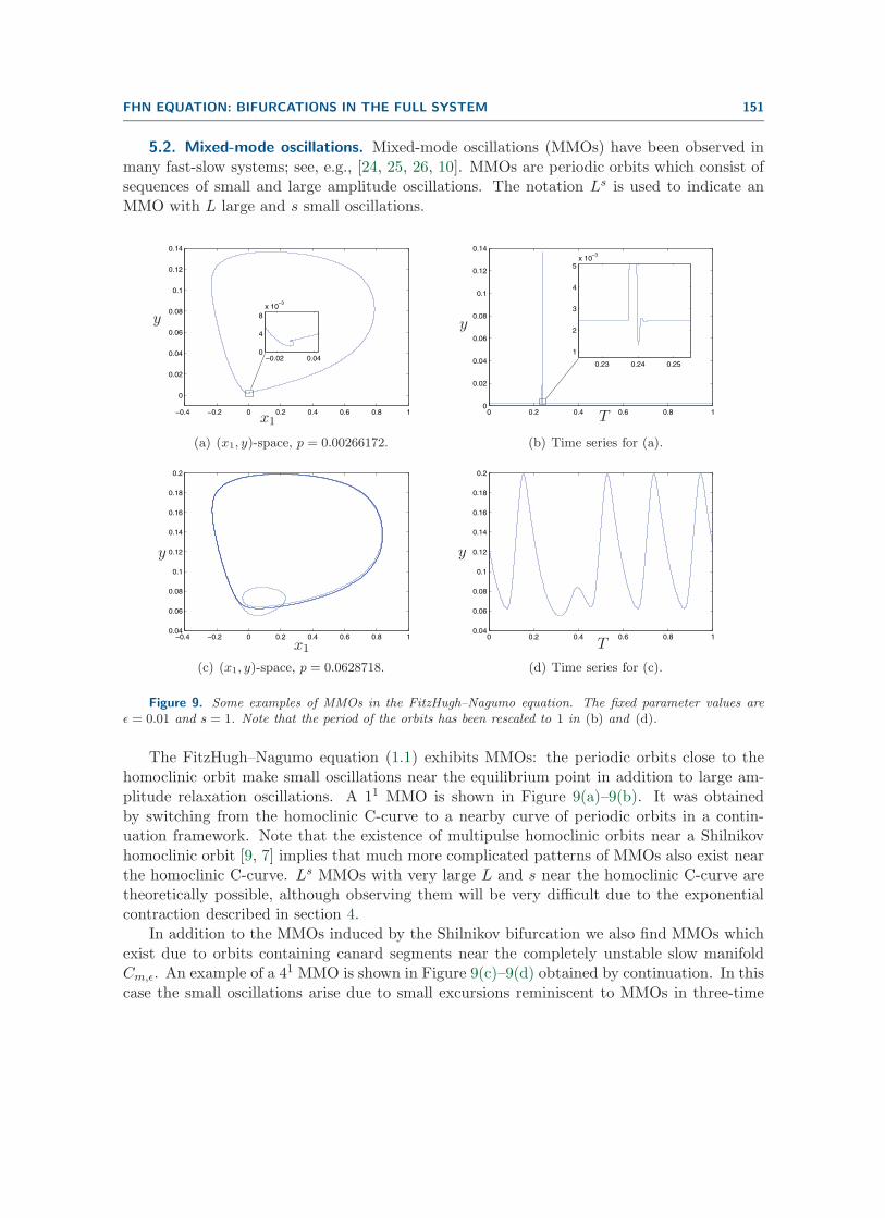
5.2. Mixed-mode oscillations. Mixed-mode oscillations (MMOs) have been observed inmany fast-slow systems; see, e.g., [24, 25, 26, 10]. MMOs are periodic orbits which consist ofsequences of small and large amplitude oscillations. The notation Ls is used to indicate anMMO with L large and s small oscillations.

−0.4 −0.2 0 0.2 0.4 0.6 0.8 1

0

0.02

0.04

0.06

0.08

0.1

0.12

0.14

−0.02 0.040

4

8x 10

−3

x1

y

(a) (x1, y)-space, p = 0.00266172.

0 0.2 0.4 0.6 0.8 10

0.02

0.04

0.06

0.08

0.1

0.12

0.14

0.23 0.24 0.25

1

2

3

4

5x 10

−3

y

T

(b) Time series for (a).

−0.4 −0.2 0 0.2 0.4 0.6 0.8 10.04

0.06

0.08

0.1

0.12

0.14

0.16

0.18

0.2

x1

y

(c) (x1, y)-space, p = 0.0628718.

0 0.2 0.4 0.6 0.8 10.04

0.06

0.08

0.1

0.12

0.14

0.16

0.18

0.2

y

T

(d) Time series for (c).

Figure 9. Some examples of MMOs in the FitzHugh–Nagumo equation. The fixed parameter values areε = 0.01 and s = 1. Note that the period of the orbits has been rescaled to 1 in (b) and (d).

The FitzHugh–Nagumo equation (1.1) exhibits MMOs: the periodic orbits close to thehomoclinic orbit make small oscillations near the equilibrium point in addition to large am-plitude relaxation oscillations. A 11 MMO is shown in Figure 9(a)–9(b). It was obtainedby switching from the homoclinic C-curve to a nearby curve of periodic orbits in a contin-uation framework. Note that the existence of multipulse homoclinic orbits near a Shilnikovhomoclinic orbit [9, 7] implies that much more complicated patterns of MMOs also exist nearthe homoclinic C-curve. Ls MMOs with very large L and s near the homoclinic C-curve aretheoretically possible, although observing them will be very difficult due to the exponentialcontraction described in section 4.

In addition to the MMOs induced by the Shilnikov bifurcation we also find MMOs whichexist due to orbits containing canard segments near the completely unstable slow manifoldCm,ε. An example of a 41 MMO is shown in Figure 9(c)–9(d) obtained by continuation. In thiscase the small oscillations arise due to small excursions reminiscent to MMOs in three-time


scale systems [16, 21]. MMOs of type L1 with L = 1, 2, 3, . . . , O(102) can easily be observedfrom continuation, and we expect that L1 MMOs exist for any L ∈ N. It is likely that theseMMOs can be analyzed using a version of the FitzHugh–Nagumo equation containing O(1),O(ε), and O(ε2) terms similar to the one introduced in [13], but we leave this analysis forfuture work.

Figure 9 was obtained by varying p for fixed values of ε = 0.01 and s = 1. Thus, varyinga single parameter suffices to switch between MMOs whose small amplitude oscillations havea different character. In the first case, the small amplitude oscillations occur when the orbitcomes close to a saddle focus rotating around its stable manifold, while in the second case,the trajectory never approaches the equilibrium and its small amplitude oscillations occurwhen the trajectory flows along the completely unstable slow manifold Cm,ε. Different typesof MMOs seem to occur very frequently in single and multiparameter bifurcation problems;see [5] for a recent example. This contrasts with most work on the analysis of MMOs [20, 25],which focuses on identifying the mechanism for generating MMOs in an example. The MMOsin the FitzHugh–Nagumo equation show that a fast-slow system with three or more variablescan exhibit MMOs of different types and that one should not expect a priori that a singlemechanism will suffice to explain all the MMO dynamics.

REFERENCES

[1] D. G. Aronson and H. F. Weinberger, Nonlinear diffusion in population genetics, combustion, andnerve pulse propagation, in Partial Differential Equations and Related Topics, Lecture Notes in Math.446, Spinger, Berlin, 1975, pp. 5–49.

[2] G. A. Carpenter, A geometric approach to singular perturbation problems with applications to nerveimpulse equations, J. Differential Equations, 23 (1977), pp. 335–367.

[3] A. R. Champneys, V. Kirk, E. Knobloch, B. E. Oldeman, and J. D. M. Rademacher, Unfolding atangent equilibrium-to-periodic heteroclinic cycle, SIAM J. Appl. Dyn. Syst., 8 (2009), pp. 1261–1304.

[4] A. R. Champneys, V. Kirk, E. Knobloch, B. E. Oldeman, and J. Sneyd, When Shil’nikov meetsHopf in excitable systems, SIAM J. Appl. Dyn. Syst., 6 (2007), pp. 663–693.

[5] M. Desroches, B. Krauskopf, and H. M. Osinga, Mixed-mode oscillations and slow manifolds in theself-coupled FitzHugh-Nagumo system, Chaos, 18 (2008), 015107.

[6] E. J. Doedel, A. R. Champneys, F. Dercole, T. Fairgrieve, Y. Kuznetsov, B. Oldeman, R.

Paffenroth, B. Sandstede, X. Wang, and C. Zhang, Auto 2007p: Continuation and Bifurca-tion Software for Ordinary Differential Equations (with Homcont), http://cmvl.cs.concordia.ca/auto(2007).

[7] J. W. Evans, N. Fenichel, and J. A. Feroe, Double impulse solutions in nerve axon equations, SIAMJ. Appl. Math., 42 (1982), pp. 219–234.

[8] N. Fenichel, Geometric singular perturbation theory for ordinary differential equations, J. DifferentialEquations, 31 (1979), pp. 53–98.

[9] S. V. Gonchenko, D. V. Turaev, P. Gaspard, and G. Nicolis, Complexity in the bifurcation struc-ture of homoclinic loops to a saddle-focus, Nonlinearity, 10 (1997), pp. 409–423.

[10] J. Guckenheimer, Singular Hopf bifurcation in systems with two slow variables, SIAM J. Appl. Dyn.Syst., 7 (2008), pp. 1355–1377.

[11] J. Guckenheimer and P. Holmes, Nonlinear Oscillations, Dynamical Systems, and Bifurcations ofVector Fields, Springer, New York, 1983.

[12] J. Guckenheimer and C. Kuehn, Computing slow manifolds of saddle type, SIAM J. Appl. Dyn. Syst.,8 (2009), pp. 854–879.

[13] J. Guckenheimer and C. Kuehn, Homoclinic orbits of the FitzHugh-Nagumo equation: The singularlimit, Discrete Contin. Dyn. Syst. Ser. S, 2 (2009), pp. 851–872.

http://cmvl.cs.concordia.ca/auto


[14] E. Hairer and G. Wanner, Solving Ordinary Differential Equations II, Springer, Berlin, 1991.[15] S. P. Hastings, On the existence of homoclinic and periodic orbits in the FitzHugh-Nagumo equations,

Quart. J. Math. Oxford Ser. (2), 27 (1976), pp. 123–134.[16] J. Jalics, M. Krupa, and H. G. Rotstein, A Novel Canard-Based Mechanism for Mixed-Mode Oscil-

lations in a Neuronal Model, http://arxiv.org/abs/0804.0829 (2009).[17] C. Jones and N. Kopell, Tracking invariant manifolds with differential forms in singularly perturbed

systems, J. Differential Equations, 108 (1994), pp. 64–88.[18] C. Jones, N. Kopell, and R. Langer, Construction of the FitzHugh-Nagumo pulse using differential

forms, in Patterns and Dynamics in Reactive Media, Springer, New York, 2001, pp. 101–115.[19] C. K. R. T. Jones, Stability of the travelling wave solution of the FitzHugh-Nagumo system, Trans.

Amer. Math. Soc., 286 (1984), pp. 431–469.[20] M. T. M. Koper, Bifurcations of mixed-mode oscillations in a three-variable autonomous Van der Pol-

Duffing model with a cross-shaped phase diagram, Phys. D, 80 (1995), pp. 72–94.[21] M. Krupa, N. Popovic, N. Kopell, and H. G. Rotstein, Mixed-mode oscillations in a three time-scale

model for the dopaminergic neuron, Chaos, 18 (2008), 015106.[22] M. Krupa, B. Sandstede, and P. Szmolyan, Fast and slow waves in the FitzHugh-Nagumo equation,

J. Differential Equations, 133 (1997), pp. 49–97.[23] M. Krupa and P. Szmolyan, Relaxation oscillation and canard explosion, J. Differential Equations, 174

(2001), pp. 312–368.[24] A. Milik and P. Szmolyan, Multiple time scales and canards in a chemical oscillator, in Multiple-

Time-Scale Dynamical Systems, C. K. R. T. Jones and A. I. Khibnik, eds., Springer, New York, 2001,pp. 117–140.

[25] H. G. Rotstein, M. Wechselberger, and N. Kopell, Canard induced mixed-mode oscillations in amedial entorhinal cortex layer II stellate cell model, SIAM J. Appl. Dyn. Syst., 7 (2008), pp. 1582–1611.

[26] J. Rubin and M. Wechselberger, The selection of mixed-mode oscillations in a Hodgin-Huxley modelwith multiple timescales, Chaos, 18 (2008), 015105.

[27] L. F. Shampine and M. W. Reichelt, The MATLAB ODE suite, SIAM J. Sci. Comput., 18 (1997),pp. 1–22.

[28] L. P. Shilnikov, A case of the existence of a denumerable set of periodic motions, Soviet Math. Dokl.,6 (1965), pp. 163–166.

http://arxiv.org/abs/0804.0829

homoclinic orbits of the fitzhughâ€“nagumo equation

Documents