wave transmission in nonlinear lattices · 3.5. normal form computation of the homoclinic tangle...

*Corresponding author.

Physics Reports 307 (1999) 333—432

Wave transmission in nonlinear lattices

D. Hennig!,*, G.P. Tsironis"! Freie Universita( t Berlin, Fachbereich Physik, Institut fu( r Theoretische Physik, Arnimallee 14, 14195 Berlin, Germany

" Department of Physics, University of Crete and Foundation for Research and Technology Hellas, P.O. Box 2208,Heraklion 71003, Crete, Greece

Received February 1998; editor: D.K. Campbell

Contents

1. Nonlinear lattice systems 3361.1. Introduction 3361.2. The discrete nonlinear Schrodinger

equation 3361.3. The Holstein model and the DNLS 3371.4. Coupled nonlinear wave guides and the

DNLS 3381.5. A generalized DNLS and nonlinear

electrical lattices 3411.6. Connection with the Holstein model 3431.7. General properties of nonlinear maps 3441.8. Integrable mappings and soliton equations 346

2. Spatial properties of integrable andnonintegrable discrete nonlinear Schrodingerequations 3482.1. Integrable and nonintegrable discrete

nonlinear Schrodinger equations 3482.2. The generalized nonlinear discrete

Schrodinger equation 3502.3. Stability and regular solutions 3512.4. Reduction of the dynamics to a two-

dimensional map 3562.5. Period-doubling bifurcation sequence 3582.6. Transmission properties 3622.7. Amplitude stability 364

3. Soliton-like solutions of the generalized discretenonlinear Schrodinger equation 3673.1. Introduction 367

3.2. The real-valued stationary problem of theGDNLS 367

3.3. The anti-integrable limit and localizedsolutions 370

3.4. The Melnikov function and homoclinicorbits 372

3.5. Normal form computation of thehomoclinic tangle 375

3.6. Homoclinic, heteroclinic orbits andexcitations of localized solutions 378

3.7. The soliton pinning energy 3823.8. Summary 385

4. Effects of nonlinearity in Kronig—Penneymodels 3874.1. Motivation 3874.2. The nonlinear Kronig—Penney model 3874.3. Propagation in periodic and quasiperiodic

nonlinear superlattices 3924.4. Wave propagation in periodic nonlinear

superlattices 3944.5. Transmission in a quasiperiodic lattice-I 4014.6. Transmission in a quasiperiodic lattice-II 4034.7. Field dependence and multistability 412

5. Conclusions 426Acknowledgements 427References 427

0370-1573/99/$ — see front matter ( 1999 Elsevier Science B.V. All rights reserved.PII: S 0 3 7 0 - 1 5 7 3 ( 9 8 ) 0 0 0 2 5 - 8

WAVE TRANSMISSION IN NONLINEARLATTICES

D. HENNIG!, G.P. TSIRONIS"

!Freie Universita( t Berlin, Fachbereich Physik, Institut fu( r Theoretische Physik, Arnimallee 14,14195 Berlin, Germany

"Department of Physics, University of Crete and Foundation for Research and Technology Hellas,P.O. Box 2208, Heraklion 71003, Crete, Greece

AMSTERDAM — LAUSANNE — NEW YORK — OXFORD — SHANNON — TOKYO

Abstract

The interplay of nonlinearity with lattice discreteness leads to phenomena and propagation properties quite distinctfrom those appearing in continuous nonlinear systems. For a large variety of condensed matter and optics applicationsthe continuous wave approximation is not appropriate. In the present review we discuss wave transmission properties inone dimensional nonlinear lattices. Our paradigmatic equations are discrete nonlinear Schrodinger equations and theirstudy is done through a dynamical systems approach. We focus on stationary wave properties and utilize well knownresults from the theory of dynamical systems to investigate various aspects of wave transmission and wave localization.We analyze in detail the more general dynamical system corresponding to the equation that interpolates between thenon-integrable discrete nonlinear Schrodinger equation and the integrable Albowitz—Ladik equation. We utilize thisanalysis in a nonlinear Kronig—Penney model and investigate transmission and band modification properties. We discussthe modifications that are effected through an electric field and the nonlinear Wannier—Stark localization effects that areinduced. Several applications are described, such as polarons in one dimensional lattices, semiconductor superlatticesand one dimensional nonlinear photonic band gap systems. ( 1999 Elsevier Science B.V. All rights reserved.

PACS: 63.10.#a

D. Hennig, G.P. Tsironis / Physics Reports 307 (1999) 333—432 335

1. Nonlinear lattice systems

1.1. Introduction

Nonlinear lattices are formed when physical properties of a system are described through aninfinite set of coupled nonlinear evolution equations. The lattice has typically spatial connotationsince, in most cases of interest, the physical system corresponds to coupled sets of linear ornonlinear oscillators distributed in space. If we are interested in phenomena with a length scalemuch larger than the typical distance between the oscillators, we can perform a continuousapproximation and obtain nonlinear partial differential equations. Many of these equations thatresult from this continuous approximation have interesting properties and lead to solitons, solitarywaves, breathers, etc. The other limit where the waves of interest are in the same scale of the typicalinteroscillator distance is also quite interesting and the corresponding wave properties are quitedistinct from those in the continuous limit. In this realm nonlinearity and discreteness conspire intoproducing localized modes as well as global lattice properties different from those of the continuousmodel. The emphasis of this review will be towards describing global lattice properties related towave transmission through one dimensional discrete nonlinear systems. We will use as ourparadigmatic equation for this review a generalized version of the discrete nonlinear Schrodinger(DNLS) equation that contains both integrable and nonintegrable terms. A major part of thereview will deal with a nonlinear version of the Kronig—Penney model with delta functions, ora nonlinear Dirac comb, that will be shown to be equivalent to a DNLS-like nonlinear lattice.

1.2. The discrete nonlinear Schrodinger equation

The DNLS or discrete self-trapping equation (DST) describes properties of chemical, condensedmatter as well as optical systems where self-trapping mechanisms are present. These mechanismsarise either from strong interaction with environmental variables or genuine nonlinear propertiesof the medium. The DNLS equation was introduced in order to describe the dynamics of a set ofnonlinear anharmonic oscillators and to understand nonlinear localization phenomena [1]. It canalso be viewed as an equation describing the motion of a quantum mechanical particle interactingstrongly with vibrations [2]. If t

n(t) denotes the probability amplitude for the particle to be at site

n of a one dimensional lattice at time t, DNLS reads:

i dtn/dt"e

ntn#»(t

n~1#t

n`1)!cDt

nD2t

n, (1)

where en

designates the local energies at site n of a one dimensional crystal, » is the nearest-neighbor wavefunction overlap and c is the nonlinearity parameter that is related to the localinteraction of the particle with other degrees of freedom of the medium. Typically an infinite,discrete set of equations, such as DNLS, is viewed in two different ways, either as a discretization ofa corresponding continuous field equation, or an equation describing dynamics in discretegeometries. In the case of DNLS, the corresponding continuous field equation is the celebratednonlinear Schrodinger equation. The present exposition will take the point of view that DNLSrepresents dynamics in a discrete one dimensional lattice. We will therefore not relate properties ofDNLS with the corresponding continuous equation.

336 D. Hennig, G.P. Tsironis / Physics Reports 307 (1999) 333—432

The DNLS equation has a long history; in its time independent form was first obtained byHolstein in his study of the polaron problem [3]. Subsequently derived in a fully time-dependentform by Davydov in his studies of energy transfer in proteins and other biological materials [4—7].Eilbeck, Lomdahl and Scott [1,8—10] studied DNLS as a Hamiltonian system of classical oscil-lators, focused on analytical and perturbative results and showed that bifurcations occur in thespace of stationary states for different values of the nonlinearity parameter. These bifurcations inthe discrete set of equations are associated with the nonlinearity induced self-trapping described byDNLS. In order to understand the dynamical properties of DNLS solutions, Kenkre, Campbelland Tsironis studied extensively the nonlinear dimer, the smallest nontrivial DNLS unit [2,11,12].The latter proved to be completely integrable and from its complete solution a number ofinteresting properties of self-trapping were obtained. Additionally, the effects of nonlinearity ona variety of physical observables were studied leading to predictions for possible experiments[13—15].

By adding to the DNLS equation a nonlinear term that is identical to the one in theAblowitz—Ladik (AL) [16] equation one obtains a combined AL-DNLS equation [17,18]:

i dtn(t)/dt"(1#kDt

n(t)D2)[t

n`1(t)#t

n~1(t)]!cDt

n(t)D2t

n(t) , (2)

where we set for simplicity en"0. We note that for c"0 Eq. (2) reduces to the integrable

Ablowitz—Ladik equation whereas in the other extreme when k"0 it becomes the nonintegrableDNLS. The combined AL-DNLS equation interpolates between these two extreme cases. In thisarticle we will deal almost exclusively with stationary properties of DNLS and DNLS-likeequations, such as the AL-DNLS equation, in extended lattice systems. Since our interest in theseproblems is motivated through physical applications we will first discuss the context in whichDNLS arises in applications.

1.3. The Holstein model and the DNLS

In order to see the connection of DNLS with the Holstein model [3] for molecular crystals westart with the Hamiltonian:

H"(K/2)+n

u2n#(1/2)M+

n

(dun/dt)2#+

n

enDnTSnD!J+

n

[Dn#1TSnD#DnTSn#1D]

!A+n

unDnTSnD . (3)

This Hamiltonian represents an excitation moving in a one-dimensional crystal while interactingwith local Einstein-type oscillators. In Eq. (3) e

nrepresents the local site energy at site n, J gives

the magnitude of the wavefunction overlap of neighboring sites, DnT and SnD are related to theprobability amplitudes at site n whereas u

nis the displacement of the n-th local oscillator. The

exciton-phonon coupling term is diagonal in the DnT basis and depends only on local oscillatordisplacements. If we neglect the kinetic energy terms and expand the time-dependent wave functionas DWT"+

pW

pDpT, where the DpT represent Wannier states. Inserting this into the time-dependent

Schrodinger equation i(dDWT/dt)"HDWT, and using the orthonormality property for the DpT’s,


we obtain:

i dWn/dt"(K/2)+

m

u2mW

n#e

nW

n!J[W

n~1#W

n`1]!Au

nW

n. (4)

Next, we eliminate the vibrational degrees of freedom by imposing the condition of minimization ofthe energy of the stationary states [3]. Inserting W

n& exp[iEt] and using the normalization

condition for the amplitudes Wp, +

pDW

pD2"1, we get

E"(K/2)+n

u2n#+

n

[en!Au

n]DW

nD2!J+

n

(Wn~1

!Wn`1

)W*n. (5)

Imposing the extremum energy condition, i.e. dE/dun"0, we obtain u

n"ADW

nD2/K. Inserting this

back into Eq. (4), we get

i dWn/dt"(A2/2K)+

p

DWpD4#e

nW

n!J[W

n~1#W

n`1]!(A2/K)DW

nD2W

n. (6)

This last step represents a departure from the Holstein adiabatic approach being valid in a limitwhere the assumed classical vibrational degrees of freedom adjust rapidly to the excitonic motion.In this anti-adiabatic limit, it is still possible to retain approximately the dynamics in the originalEq. (4). The quantity (A2/2K)+

pDW

pD4 represents the total vibrational energy. If we measure

energies with respect to this background value, we arrive at an effective nonlinear equation for theamplitude W

n(t):

i dWn/dt"e

nW

n!J[W

n~1#W

n`1]!(A2/K)DW

nD2W

n. (7)

This closed nonlinear equation describes the effective motion of the “polaron” in the aforemen-tioned anti-adiabatic limit. The “time step” dt in the time derivative should be understood as shortcompared to the time scale of the “bare exciton motion” (proportional to 1/J) but long comparedto the fast vibrational motion (proportional to 1/K).

1.4. Coupled nonlinear wave guides and the DNLS

In the previous section we showed how DNLS can be motivated in a solid-state context. In anoptics context, DNLS describes wave motion in coupled nonlinear waveguides. When an electro-magnetic wave is sent through a nonlinear waveguide coupled to other waveguides in its vicinity,W

nrepresents the amplitude coefficient in an expansion of the electromagnetic field in terms of

the wave normal modes in the waveguide. Coupling causes power to be exchanged amongthe waveguides. The nonlinear nature of the materials in each waveguide (coupler) can cause a“trapping” of power in one of the waveguides. Self-trapping now happens in space rather than intime. These features could be exploited in the design of optical ultrafast switches with applicationsin optical computers [19,20].

Nonlinear couplers arranged in various geometries are known to have properties that makethem attractive candidates for all optical switching devices. In Fig. 1 we show a typical configura-tion for an array of such couplers. The basic nonlinear coupler model, introduced by Jensen in1982, involves two waveguides made of similar optical material embedded in a different hostmaterial [19]. The waveguides have strong nonlinear susceptibilities whereas the host is made out


Fig. 1. A system of coupled nonlinear waveguides extending in the z-direction.

of material with a purely linear susceptibility. The host enables interaction between the modespropagating in the two waveguides whereas the nonlinear susceptibility gives rise to the phenom-enon of mode self-trapping in each waveguide. For a device of a given length, the launching ofpower in one side of the device can give a wide range of amplitudes in each guide. For sufficientlylarge values of power, the nonlinear susceptibility terms dominate and we have almost completeself-trapping of the energy in the initially excited guide. Switching is possible for a variety ofdifferent initial electric field amplitudes in both waveguides [19,21].

We assume an extended system involving many couplers distributed as in Fig. 1 and performnormal mode analysis. From [19], the amplitude a(n)k of the kth mode of the nth guide, obeys theequation

!ida(n)kdz

"

u4PkPdx dyE(n)k )P @ , (8)

where the axes of the guides are along z, E(n)k is the electric field of the kth mode in the nth guide,Pk is the power in the kth mode and P @ is the perturbing polarization due to linear and nonlineareffects. For the nth guide,

P @/e0"E(n)d#(d#e)[E(n`1)#E(n~1)]#s(3)[DE(n)D2#DE(n~1)D2#DE(n`1)D2]E(n) , (9)

in which e is the dielectric coefficient of the host material, e#d that of the guide material and s(3) isthe third-order susceptibility [22]. E(i) is the total field due to the ith guide. Eq. (8) then gives

!ida(n)kdz

"

ue0

4PkPdx dy[dE(n)*k )E(n)#(e#d)E(n)*k ) (E(n~1)#E(n`1))

#s(3)(DE(n)D2#DE(n~1)D2#DE(n`1)D2)ME(n)*k )E(n)N] . (10)


Similar equations hold for guides (n!1) and (n#1). Expanding the total fields in normal modes,Eq. (10) gives a set of mode-coupled equations for the mode amplitudes. If we assume only thelowest single-mode operation for each guide, so that E(n)"a(n)k E(n)k etc. for E(n~1) and E(n`1), thenEq. (10) with k"1, gives the following set of equations:

!i da(n)1

/dz"Q(n)1

a(n)1#Q

n,n~1a(n~1)1

#Qn,n`1

a(n`1)1

#Q(n)3

Da(n)1

D2a(n)1

. (11)

The coefficients are given by

Q(n)1"

ue0

4P Pdx dy dDE(n)D2 , (12)

Q(n)3"

ue0

4Ps(3)Pdxdy dDE(n)D4 , (13)

Qnl"

ue0

4P Pdx dy(e#d)E(n)* )E(l), (nOl ) . (14)

The coupling coefficient Qnl

for nOl is generally complex due to the phase mismatch associatedwith the assumed mode factor exp(ibkz). The latter factor enters in a normal mode expansion

E(n)"+k

a(n)k exp(ibkz)E(n)k

for each mode, with bk being the wave vector of propagation of the kth mode propagating in thez direction. The inner product in the integrand of Eq. (14) may be positive or negative dependingon the polarization direction in each waveguide respectively. In the general case of dissimilarwaveguides (say guides n and n!1) phase mismatch will result in spatially modulated Q

n,n~1terms

proportional to exp(iDbz), with Db the difference of the wavevectors of the waves propagating inthe two waveguides respectively. When the waveguides are taken to be identical, Db"0 and spacemodulation is not present. Additionally, with the present boundary conditions at z"0, the innerproduct in Eq. (14) is positive and as a result Q

n,n~1is real and positive. If, on the other hand, phase

mismatch leads to a spatial Qn,n~1

modulation much faster than the mode amplitude change overthe length of the waveguide, an average effective Q

n,n~1can be used. An average of a rapidly

oscillating factor exp(iDbz) over the device length ¸ leads, in general to a complex Qn,n~1

term,whose actual value depends on the product (Db)¸. In this context, it is possible to choose values ofDb that give rise to a real but negative effective Q

n,n~1term resulting in more abrupt switching

properties. Taking Qn,n~1

real, then Qn,n~1

"Qn~1,n

and by symmetry then Qn,n`1

"Qn`1,n

.Defining Q

n,n~1"Q

n,n`1"!», Eq. (11) can now be written as

!ida(n)

dz"Q

1a(n)!»(a(n~1)#a(n`1))#Q

3Da(n)D2a(n) , (15)

where the subscript 1 in the variables a(i)1

was dropped. Now letting

a(n)"cnJP exp(iQ

nz) , (16)


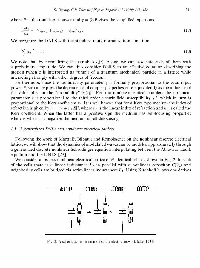
Fig. 2. A schematic representation of the electric network (after [23]).

where P is the total input power and c"Q3P gives the simplified equations

idc

ndz

"»(cn`1

#cn~1

)!cDcnD2c

n. (17)

We recognize the DNLS with the standard unity normalization condition

+p

DcpD2"1 . (18)

We note that by normalizing the variables ci(z) to one, we can associate each of them with

a probability amplitude. We can thus consider DNLS as an effective equation describing themotion (when z is interpreted as “time”) of a quantum mechanical particle in a lattice whileinteracting strongly with other degrees of freedom.

Furthermore, since the nonlinearity parameter c is formally proportional to the total inputpower P, we can express the dependence of coupler properties on P equivalently as the influence ofthe value of c on the “probability” Dc

i(z)D2. For the nonlinear optical couplers the nonlinear

parameter s is proportional to the third order electric field susceptibility s(3) which in turn isproportional to the Kerr coefficient n

2. It is well known that for a Kerr type medium the index of

refraction is given by n"n0#n

2DED2, where n

0is the linear index of refraction and n

2is called the

Kerr coefficient. When the latter has a positive sign the medium has self-focusing propertieswhereas when it is negative the medium is self-defocusing.

1.5. A generalized DNLS and nonlinear electrical lattices

Following the work of Marquie, Bilbault and Remoissenet on the nonlinear discrete electricallattice, we will show that the dynamics of modulated waves can be modeled approximately througha generalized discrete nonlinear Schrodinger equation interpolating between the Ablowitz—Ladikequation and the DNLS [23].

We consider a lossless nonlinear electrical lattice of N identical cells as shown in Fig. 2. In eachof the cells there is a linear inductance ¸

2in parallel with a nonlinear capacitor C(»

n) and

neighboring cells are bridged via series linear inductances ¸1. Using Kirchhoff ’s laws one derives


a system of nonlinear discrete equations containing the nonlinear electrical charge Qn(t) of the nth

cell and the corresponding voltage »n(t):

d2Qn/dt2"(1/¸

1)(»

n`1#»

n~1!2»

n)!(1/¸

2)»

n, n"1, 2,2 . (19)

We assume further for the charge a voltage dependence similar to that of an electrical Toda lattice[24,25]

Qn(t)"AC

0ln[1#»

n/A] , (20)

which is justified if the inverse of the nonlinear capacitance follows a linear relation [26] accordingto

1/C(»n)"(A#»

n)/AC

0. (21)

With the help of Eq. (19) one obtains the linear dispersion relation typical for a bandpass filter

u2"u20#4u2

0sin2(k/2) , (22)

where u20"1/¸

2C

0and u2

0"1/¸

1C

0. Due to the lattice discreteness the spectrum is bounded from

above by a cutoff frequency f.!9

"u.!9

/2p"(u20#4u2

0)1@2.

Inserting the expression for Qnof Eq. (20) into Eq. (19) one obtains [23]

(A#»n)d2»

ndt2

!Cd»

ndt D

2"

u20

A(A#»

n)2C»n`1

#»n~1

!A2#u2

0u20B»nD . (23)

Discreteness of the lattice is maintained for a gap angular frequency u0much larger than any other

frequency of the system, i.e. u20<4u2

0. Using this fact, we can neglect all the harmonics of a wave

with any frequency f since they lie above the cutoff frequency. Therefore the study is restricted toslow temporal variations of the wave envelope and solutions of the form

»n(t)"eW

n(¹) exp(!iut)#eW*

n(¹) exp(#iut) , (24)

are searched for and e is a small parameter rescaling the time unit as ¹"e2t. Upon substitutingthis expression in Eq. (23) and retaining only terms of order e2 we arrive at

2u2

u20

DWnD2W

n"!CWn`1

#Wn~1

!A2#u2

0u20BWnDDWn

D2

!CW*n`1

#W*n~1

!A2#u2

0u20BW*

nDW2n

. (25)

Collecting now terms in exp(!iut), setting q"u20¹/2u and W

n"U

nexp[iq(u2!u2

0!2u2

0)/u2

0]

gives finally

idU

ndq

#[Un`1

#Un~1

]#[k(Un`1

#Un~1

)!2lUn]DU

nD2"0 , (26)

with parameters

k"1A2

, l"2u2#u2

0#2u2

02u2

0A2

. (27)


With the help of the generalized discrete nonlinear Schrodinger equation Remoissenet et al.demonstrated theoretically the possibility for the system to exhibit modulational instability leadingto a self-induced modulation of an input plane wave with the subsequent generation of localizedpulses. In this way energy localization in a homogeneous nonlinear system is possible and ismanifested in the formation of envelope solitons [26]. Experimentally these results are confirmedby the observation of a staggered localized mode in the real electrical network.

1.6. Connection with the Holstein model

We saw previously how the nonlinear nonlocal term of the AL-DNLS equation arises in thecontext of the electrical lattice. Given the connection of DNLS with the Holstein model, it makessense to ask whether this nonlocal term could be also associated with that model as well in someform. It is customary to view the nonlinear term in the pure DNLS equation as being associatedwith a local energy distortion that arises variationally from the adiabatic elimination of vibrationaldegrees of freedom. The AL equation, on the other hand, does not carry a similar physicalinterpretation in this context. We can, however, identify the physics behind the interpolatingAL-DNLS equation in a more precise way, starting from an extension of the one-electron HolsteinHamiltonian. We assume that an electron is moving in a one dimensional tight-binding lattice withnearest neighbor matrix elements J while at the same time interacts with local Einstein oscillatorsof mass M and frequency u

E. The oscillators modulate both the local electron energies (as in the

conventional Holstein model) but also affect the transfer rates; we assume that the modification ofthe rate between adjacent sites is determined through the average local oscillator distortion. Wehave the following Hamiltonian:

HH"

12M+

n

(yR 2n#u2

Ey2n)!J+

n

(a`n

an`1

#a`n`1

an)

!a+n

yna`n

an,!b+

n

(yn`1

#yn)(a`

n`1an#a`

nan`1

) , (28)

where a`n

, an

are the electron creation and annihilation operators at site n respectively, yn

is thedisplacement of the local Einstein oscillator in the same site and a,b are coupling parameters. Wenote the physical significance of the additional interaction contribution that are proportional to b:the two terms proportional to y

n`1a`n`1

an#y

na`n

an`1

correspond to the modulation of thetransfer rate as a result of the distortion in the “destination site” whereas the other two termsdepend on the distortion in the originating site.

We proceed now and perform the same adiabatic elimination of the vibrational degrees offreedom as in Section 1.3. After some straightforward manipulations and keeping only termsproportional to a2, ab but not of the order of b2 results in the following stationary equation for theenergy E:

Eam"(a

m`1#a

m~1)!cDa

mD2a

m#k(a

m`1#a

m~1)Da

mD2#O(ab)#O(b2)#2 , (29)

where we set J"!1, c"a2/(MuE),k"2ab/(Mu

E) and we designated with O(ab) the terms

O(ab)"k[(a*m`1

#a*m~1

)a*m#Da

m`1D2a

m`1#Da

m~1D2a

m~1]. These last terms that are also of order

k are the modification to the transfer rate due to the local deformation in the originating site.


Clearly, if these terms are absent, the resulting equation becomes the stationary equivalent of theAL-DNLS equation. Consequently, the physical significance of the AL-type terms becomestransparent: they correspond to the modification in the transfer rates when the local distortion istaken only partially into account and depends only on the modification at the landing site.Furthermore, since dropping the terms O(ab) is equivalent to dropping two of the interaction terms(out of the four), the resulting nonhermitianity of the problem is manifested in the existence ofa norm which is different from the usual probability norm of DNLS. It is easy to check that if allfour terms are kept, the resulting nonlinear equation has a probability norm.

1.7. General properties of nonlinear maps

The study of the stationary properties of DNLS-like equations will be done through the use oftwo dimensional nonlinear maps. By now there exists a vast literature on maps (see e.g. [27—31]).We restrict ourselves to give a brief overview and summarize the basic features of such mapsnecessary for an analysis of the physical properties of the underlying nonlinear lattices once theyhave been casted into discrete maps. Nonlinear maps are used in a variety of properties rangingfrom stability studies of colliding particle beams in storage rings [32—35], to Anderson localization[36—39] and commensurate—incommensurate structure studies in solid state physics [40—42].

A map ¹ of the plane generates a sequence of points xn"(x

n, y

n)3R2, n"0, 1, 2,2 by assigning

to each point xn

of the plane a new point via xn`1

"¹(xn). The entire sequence x

nwith

n"0, 1, 2,2 is called an orbit. The map ¹ is said to be area-preserving if for any given measurablesubset » of the plane, ¹~1(») has the same area as ». This condition becomes equivalent to thatthe determinant of the Jacobian is one, i.e.

Det(D¹)"1 , (30)

for all x and D is the differential operator (/x, /y).We begin the discussion of the motion on the map plane with an important class of orbits,

namely periodic orbits. An orbit is periodic with period q if

xq"x

o#p, y

q"y

o, (31)

for some integer p. We denote such an orbit by (p,q). For area-preserving maps we distinguish threetypes of periodic orbits depending on the stability properties of points in their neighborhood, viz.elliptic, hyperbolic (regular saddle), and reflection hyperbolic (flip saddle). The stability is deter-mined by the eigenvalues of the tangent map. Mapping a linearized periodic orbit through itswhole period in tangent space is achieved by the product of the local Jacobians taken at eachperiodic point

(D¹)q(xo)"

q~1<n/0

D¹(xn) . (32)

Since the determinant of each local Jacobian D¹(xn) is one the determinant of any product of them

is also one. This implies that the eigenvalues j of (D¹)q are either conjugate points on the unit circleor appear as real reciprocal numbers j,1/j. The eigenvalues are connected with the trace of the


tangent map (D¹)q via

j"12[Tr(D¹)q$J[Tr(D¹)q]2!4] . (33)

The stability condition becomes thus DTr(D¹)qD(2. But a stability classification is most conve-niently given in terms of Greene’s residue [43]:

R"

14[2!Tr(D¹)q] . (34)

We summarize the results as follows [31]:

Stability j Tr(D¹)q R

Elliptic exp(2p iu) (!2, 2) (0, 1)Hyperbolic '0 '2 (0ReflectionHyperbolic (0 (!2 '1

Nearby points of each elliptic periodic point rotate about the point in ellipses by an angularincrement arccos[1!2R] on average per iteration of the map (D¹)q. Equivalently the rotationfrequency u is linked with the value of the residue via R" sin2(pu). For irrational u the orbitnever returns to its initial point and such an orbit is called quasiperiodic. The orbit points come tolay on invariant closed curves. According to the Kolmogorov—Arnold—Moser (KAM) theorem theorbit is stable provided RO0, 3/4, 1/2. For the cases of R"0, 3/4, 1/2 corresponding to the socalled Arnold resonances the linearization does not suffice for a stability analysis [44].

For R(0, where the points of the periodic orbit are hyperbolic, nearby points diverge fromthem with an exponential separation rate D1!2R#2JR2!RD.

Upon varying a parameter of the map the location of the periodic orbit as well as its residue willbe changed. If the residue changes from a positive value to the negative range then a tangentbifurcation takes place where an elliptic point handles its stability over to a hyperbolic point.Whenever the residue passes the value of one from below (if u"1/2) a stable elliptic orbit convertsinto an unstable hyperbolic point with reflection accompanied by the creation of two new stableelliptic points via a period-doubling bifurcation. The latter remain stable until the correspondingvalue of u reaches one half and another period doubling bifurcation occurs destroying also thenearby quasiperiodic orbits. After a cascade of such period doubling bifurcations local chaosappears. The character of motions on the map depends on the initial conditions. In general wedistinguish regular (integrable) and irregular (chaotic) regimes for a map. A map is said to beintegrable in the Liouville sense if there exists a sufficient number of integrals. An integral isa function on the map-plane I(x), which is invariant under the map, that is ¹(I(x))"I(x). Moreprecisely, if a 2N-dimensional map possesses N independent integrals I

j, j"1, 2,2, N which are in

involution, i.e. all the mutual Poisson brackets vanishes MIn, I

mN"0, then the motion is integrable

and lies on a family of N-dimensional nested tori appearing in the case of N"2 as closed invariantcurves.


We discuss now the transition from regular behavior to the occurrence of global chaos ina two-dimensional area-preserving map. Applying a small nonintegrable perturbation to anintegrable map the KAM theorem assures the survival of most of the invariant tori for sufficientlyweak perturbations. However, some of the invariant tori, namely those with rotational frequencyu close enough to a rational value, will break up into resonance chains (Poincare—Birkhoff-chains).These resonance chains consist of periodic points of alternating stability type. The elliptic pointsare again surrounded by stable quasiperiodic cycles. The stable and unstable manifolds belongingto the unstable hyperbolic points embrace the stability zones around the elliptic points and anisland like structures are formed called resonances. In the vicinity of the hyperbolic points localstochasticity (chaos) occurs due to the tangling of the invariant stable and unstable manifolds.

With further increase in the perturbation strength the width of the resonance islands grows andthe resonant cycles break up giving birth to new resonance chains of higher order while the otherquasiperiodic cycles remain stable due to the KAM theorem. We find local regions of regular andirregular motions coexisting on the map plane exhibiting a complicated hierarchical structure ofislands within islands. At the same time with increased island width KAM cycles lying in betweentwo neighboring resonances can be destroyed as a result of resonance overlap. When furtherincreasing the nonintegrability parameter a very complicated network of orbits develops wheremore and more regions are covered by chaotic orbits. Finally, above a critical perturbationstrength even the most resisting final KAM cycle breaks up and the phase plane will be denselycovered with global chaos except for a few tiny islands of stability.

There exists a useful property for a special class of area-preserving maps. If the map ¹ factorsaccording to ¹"¹

1¹

2, with ¹

1and ¹

2being orientation-reversing involutions, i.e. they satisfy

¹21"¹2

2"1, det(D¹

1)"det(D¹

2)"!1 , (35)

then ¹~1"¹2¹

1. That the map ¹ can be written as the product of two orientation-reversing

involutions establishes its reversibility. The invariant sets of the two involutions form the symmetrylines of the map. For reversible area-preserving maps there exists a particular symmetry line onwhich at least one point of every positive residue Poincare—Birkhoff orbit (elliptic or reflectionhyperbolic) lays. This line is called the dominant symmetry line. For reversible area-preserving mapsit suffices therefore a one-dimensional search for the periodic orbits. Furthermore one can provethat the homoclinic orbits belonging to the (transversal) intersections of the stable and unstablemanifolds of a hyperbolic point fall on symmetry lines in reversible area-preserving maps [45]. Thenext section is devoted to integrable maps since they are of importance both for the study of solitonequations as well as serve as the starting point for perturbation theory (see e.g. [46]).

1.8. Integrable mappings and soliton equations

We review the properties of nonlinear integrable maps describing the solution behavior ofcertain kinds of (stationary) solutions of nonlinear integrable lattices. Integrable partial differenceequations or nonlinear integrable lattices may arise from space discretization of integrablenonlinear partial differential equations giving differential-difference (DD) equations. The latter giverise to hierarchies of integrable PDEs [47] and are of importance especially from the point of viewof integrability in classical nonlinear Hamiltonian systems in general. Many physical systems areclose to integrable systems so that their study is also of practical interest to follow e.g. bifurcations


and the transition to chaos with a perturbational approach [48]. Furthermore, nonlinear integr-able maps are also of interest for the construction of numerical integration schemes of nonlinearPDE’s [49,50].

The oldest example of a nonlinear integrable map is certainly Jacobi’s celebrated elliptic billiard[51]. Quispel et al. [52,53] reported on an eighteen-parameter family of nonlinear integrable mapswhich is actually a generalization of the four-parameter family found by McMillan [54]. Theauthors established a linkage of these maps to soliton theory and statistical mechanics. Theytreated in detail various examples of physical interest, namely the stationary reductions of a DDisotropic Heisenberg spin chain, and besides the discrete modified Korteweg—de Vries equation,and the integrable DD nonlinear Schrodinger equation, viz. the Ablowitz—Ladik equation. All ofthese stationary soliton equations are described by symmetric integrable maps. We summarize heretheir results for the discrete modified Ablowitz—Ladik equation (»"1):

idt

ndt

"tn`1

#tn~1

#kDtnD2[t

n`1#t

n~1] . (36)

The stationary solutions follow from the ansatz tn"/

nexp(!iut) with real /

n, yielding a two-

dimensional map

u/n!(1#/2

n)[/

n`1#/

n~1]"0 . (37)

This map was studied by Ross and Thompson [55]. The map possesses the following integral ofmotion

u/n`1

/n!(1#k/2

n)/2

n`1/2

n"K , (38)

where K is the integration constant. Particularly for K"0 we obtain the separatrix solutioncorresponding to the stationary AL-soliton

/n" sinhb sinh[b(n!x

0)] , (39)

where b is a parameter and x0

specifies the soliton center.Since this map can be written as the product of two involutions it is a reversible map. It turns out

to be a special case of the eighteen-parameter family of integrable reversible planar maps given by

/n`1

"

f1(/

n)!/

n~1f2(/

n)

f2(/

n)!/

n~1f3(/

n), (40)

where

f (U)"(M0U)](M

1U) , (41)

with U"(/2,/, 1)T and

Mn"A

an

bn

cn

dn

en

fn

in

jn

knB, n"0, 1 . (42)


Each member of this family possesses a one-parameter family of invariant curves fulfilling therelation

(a0#Ka

1)/2

n`1/2

n#(b

0#Kb

1)(/2

n`1/

n#/2

n/

n`1)#(c

0#Kc

1)(/2

n`1#/2

n)

#(e0#Ke

1)/

n`1/

n#(f

0#Kf

1)(/

n`1#/

n)#(k

0#Kk

1)"0 . (43)

A parameterization of this equation in terms of Jacobian elliptic functions is possible and independence of the integration constant periodic, quasiperiodic as well as solitonic solutionbehavior can be distinguished.

There exist many more examples for differential-difference equations (DDE) the stationarysolutions of which are determined by a map of the type of (40)—(43). This led Quispel et al. to thefollowing conjecture: “Consider a differential-difference equation. ¹hen every autonomous differenceequation obtained by an exact reduction of the DDE is an integrable mapping”. However one shouldbe aware that the reverse of this conjecture does not necessarily hold [52]. On the other hand, formany physically relevant problems the solutions cannot be given at all in closed analytical formand rather irregular (chaotic) dynamics is encountered pointing to nonintegrability as it is the casealso for DNLS.

2. Spatial properties of integrable and nonintegrable discrete nonlinear Schrodinger equations

2.1. Integrable and nonintegrable discrete nonlinear Schrodinger equations

The nonlinear Schrodinger equation (NLS) is one of the prototypical nonlinear partial differen-tial equations, the study of which has lead to fundamental advances in nonlinear dynamics. Thestudy of NLS was motivated by a large number of physical and mathematical problems rangingfrom optical pulse propagation in nonlinear fibers to hydrodynamics, condensed matter physicsand biophysics. We now know that NLS provides one of the few examples of completely integrablenonlinear partial differential equations [56]. Since most work in nonlinear wave propagationinvolves at some stage a numerical study of the problem, the issue of the discretization of NLS wasaddressed early in Ref. [56]. Ablowitz and Ladik noticed that among a large number of possiblediscretizations of NLS there is one that is also integrable [16]. The study of the integrable versionof the discrete nonlinear Schrodinger equation, called hereafter Ablowitz—Ladik, or AL equation,showed that it has solutions which are essentially the discrete versions of the NLS solitons [16].Another discrete version of the NLS equation was studied in detail later [1]; the latter usuallyreferred to as discrete nonlinear Schrodinger equation DNLS or discrete self-trapping equation(DST), has quite a number of interesting properties, but it is not integrable [50]. We note that themotivation for studying the two discrete versions of NLS, viz., the AL equation and the DNLSequation respectively, are quite different: The AL equation, on one hand, has very interestingmathematical properties, but not very clear physical significance; the introduction of the DNLSequation, on the other hand, is primarily motivated physically. In particular, the latter seems toarise naturally in the context of energy localization in discrete condensed matter and biologicalsystems as well as in optical devices [1—7,57—67]. Even though in these problems one typicallyassumes that the length scale of the nonlinear wave is much larger than the lattice spacing andtherefore NLS provides a good description for those problems, the study of DNLS (and AL)


equation is important when the size of the physical system is small or the nonlinear wave is stronglylocalized.

The motivation for the present chapter is an equation introduced by Salerno [17] and studiedrecently by Cai et al. [18] that interpolates between DNLS and AL equations while containingthese two as its limits [17]. By varying the two nonlinearity parameters of this new equation one isable to monitor how “close” it is to the integrable or nonintegrable version of the NLS. The newequation finds its physical explanation in the context of the nonlinear coupler problem [68] andthe application in a nonlinear electrical transmission line [23]. However, its basic merit is that itallows us to study the interplay of the integrable and nonintegrable NLS-type terms in discretelattices. In addition, one can address the issue of “nonlinear eigenstates” of the new equation andtheir connection to the integrability/nonintegrability issue.

Before presenting the basic properties of the stationary (generalized) DNLS we give a review ofother papers on it: Salerno [17] studied the quantum deformation of AL-DNLS and derived for thetwo-particle chain (a dimer) some explicit formulas for the first excited levels of the quantizedversion showing that they can be continuously deformed into the corresponding ones of the twoextreme limits of c"0 respectively k"0. Kivshar and Peyrard obtained the DNLS in their studyof modulational instability in the discrete nonlinear Klein—Gordon lattice [69]. The DNLSarises there as the envelope function in a rotating wave approximation for slowly modulatedcarrier waves of the Klein—Gordon field amplitudes. Furthermore, for comparison they studiedalso the AL equation. Claude et al. investigated the creation and stability of localized modes inFermi—Pasta—Ulam chains and nonlinear discrete Klein—Gordon lattices [70]. Their ansatz func-tion for localized modes resulted in the DNLS. For a perturbational approach they wrote DNLS asa perturbed AL system yielding the AL-DNLS equation. Cai et al. studied the AL-DNLS equationfocusing interest on the interplay of integrability and nonintegrability [18]. They pointed out thatthe localized states of the AL system are the AL-solitons. Furthermore they showed that forAL-DNLS there exist two types of localized modes. One type is a state with in-phase oscillations ofneighboring particles having oscillation frequencies lying below the linear phonon band and iscalled an unstaggered state. The other one exhibits out-of-phase oscillations of neighboringparticles and has oscillation frequencies above the linear (phonon) band and is called a staggeredstate. For further discussion of localized (stationary) states in DNLS we refer to Section 3. Kivsharand Salerno studied analytically and numerically modulational instability for the AL-DNLSwith emphasis on how different discretizations of the nonlinear interaction term change modula-tional instability in the lattice [71]. Hays et al. studied a generalized lattice with equationiAQ

j#F(DA

jD2)(A

j`1#A

j~1)#F(DA

jD2)A

j"0 that contains DNLS, AL and several other models

as special cases. They developed a fully nonlinear modulation theory for harmonic plane wavesolutions of the form A

n(t)"a exp[i(kn!ut)] [72]. Konotop et al. [73] and Cai et al. [74] proved

integrability of the dynamics of the AL system in a time-varying, spatially uniform electric fieldalong the chain direction which is of the form »

n"E(t) n. In the limit of a static electric field, the

system exhibits a periodic evolution which is a nonlinear counterpart of Bloch oscillations. Furtherit was shown that for certain strengths of a harmonic field dynamical localization can be causedwhich can be interpreted as a parametric resonance effect. (We refer also to Section 4.7 fora treatment of similar effects in Kronig—Penney models.) Cai et al. extended the (integrable) ALsystem study by incorporating the integrability-breaking DNLS term as well and showed thatBloch oscillations and dynamical localization are maintained in the AL-DNLS system. Hence they


are effects of the lattice and does not depend on integrability. The special case of a AL system witha potential depending linearly on the spatial coordinate, i.e. »

n"An, was treated Scharf and

Bishop by means of the inverse scattering transform. These authors obtained a UV pair provingintegrability of the model [75]. Hennig et al. investigated the formation of breatherlike impuritymodes in a “disordered” version of the AL-DNLS containing a single impurity [76]. An interestingstudy on soliton interactions and beam steering in nonlinear waveguide arrays modeled by DNLSwas performed by Aceves and co-workers in Refs. [77—79]. Special attention is paid to the existenceand control of the propagation of stable localized wave packets in waveguide arrays. It is shownthat localized modes with energy stored only in a few lattice sites are the preferred stable steadypatterns of the system. Among several analytical methods (discrete variational approaches) alsosoliton perturbation theory based on a perturbed AL system was used. The issue of perturbationtheory of discrete nonlinear Schrodinger equations was also addressed in [80].

2.2. The generalized nonlinear discrete Schrodinger equation

The main purpose of this section is to study the stationary properties of the following generalizeddiscrete nonlinear Schrodinger equation (GDNLS)

i dtn(t)/dt"(»#kDt

n(t)D2)[t

n`1(t)#t

n~1(t)]!cDt

n(t)D2t

n(t) , (44)

where tnis a complex amplitude, k and c are nonlinearity parameters and » is the transfer matrix

element coupling adjacent oscillators at site n and n$1, respectively. We note that Eq. (44)interpolates between two possible discretizations of NLS viz. the DNLS and AL equation obtainedby setting k"0 (with cO0) and c"0 (with kO0), respectively [17]. To reduce the number ofparameters we use a time scaling according to »tPt and introduce the ratios cJ"c/» andkJ "k/». For ease of notations we drop the tildes afterwards. We remark that a linear contributionet

n(t) appearing on the right hand side (r.h.s.) of the Eq. (44) can be removed by a global phase

transformation tn(t)Pexp(!iet)t

n(t).

The stationary equation is obtained by substituting tn(t)"/

nexp(!iEt) in Eq. (44) giving

E/n!(1#k D/

nD2)[/

n`1#/

n~1]#cD/

nD2/

n"0 , (45)

with complex variables /nand E is the phase of the stationary ansatz. The stationary equation (45)

was analyzed in the aforementioned extreme limits through map approaches in Refs. [52,81,82].The stationary real-valued AL system satisfies an integrable mapping which is contained in the18-parameter family of integrable mappings of the plane reported by Quispel et al. in [53]. In thissection we will present an analysis of Eq. (45) and discuss the interplay of the integrable andnonintegrable nonlinear terms in the context of the complete equation [83].

Eq. (45) may be rewritten as

/n`1

#/n~1

"

E#cD/nD2

1#kD/nD2

/n

, (46)

which obviously reduces to a degenerate linear map if c"Ek. Although reduction of the complex-valued amplitude dynamics to a two-dimensional real-valued map is possible, (see Section 2.4), weconcentrate in this section on the study of the recurrence relation /

n`1"/

n`1(/

n,/

n~1) appropri-

ate for the investigation of stability of the nonlinear lattice chain. Eq. (46) can also be derived as the


relation which makes the action functional

F"+nG1kAE!

ckB ln(1#kD/

nD2)#

ckD/

nD2!(/*

n/

n`1#/

n/*n`1

)H (47)

an extremum. In the limit k"0, the latter is replaced by

F"+n

MED/nD2#1

2cD/

nD4!(/*

n/n`1

#/n/*

n`1)N . (48)

The extremal sets M/nN define the orbits and together with appropriate boundary conditions

determine the solutions of a particular physical problem. However, concerning the stabilityproperties one has to distinguish between the (dynamical) stability of the physical solutions and the(linear mapping) stability of the corresponding map orbit generated by the recurrence relation/n`1

"/n`1

(/n, /

n~1) [41,42]. In general, a dynamical stable solution minimizing the action

corresponds to a linearly unstable map orbit, whereas physically unstable solutions correspondingto maximum energy configurations are reflected in the map dynamics as linearly stable orbits. Inthe present study we focus on the transmission properties of the “nonlinear lattice” of Eq. (45),since finding the linearly stable map solutions (propagating wave solutions) is essential.

2.3. Stability and regular solutions

The second-order difference equation (46) can be regarded as a symplectic nonlinear transforma-tion relating the amplitudes in adjacent lattice sites. This transformation can be considered asa dynamical system where the lattice index n plays the role of the discrete time n. The resultingdynamics of the two-component (amplitude) vector (/

n`1, /

n)T is determined by the following

Poincare map:

Mn: A

/n`1/

nB"C

En

!1

1 0 DA/

n/

n~1B , (49)

where the nonlinear transfer matrix depends on the amplitude /nthrough

En"

E#cD/nD2

1#kD/nD2

. (50)

The stability of the orbits M/nN, (n"0,2, N), or equivalently the transmission properties of the

nonlinear lattice of chain length N, is governed by the solution behavior of the correspondinglinearized equations in the neighborhood of an orbit ranging from (/

0, /

1) to (/

N~1, /

N). For

a semi-infinite (or infinite) one-dimensional lattice chain the (finite) sequence M/nN, (n"0,2,N),

defines an orbit segment.To investigate the linear stability of a given orbit we introduce a small (complex-valued)

perturbation un

and consider the perturbed orbit /nP/

n#u

n. Linearizing the map equations

results in the second-order difference equation for the perturbations un:

un`1

#un~1

"

1(1#kD/

nD2)2

M(E#2cD/nD2#kcD/

nD4)u

n#(c!Ek)/2

nu*nN . (51)


Writing further /n"A

n#iB

nand u

n"x

n#iy

nwith real A

n,B

n,x

n, y

n, we obtain the four-dimen-

sional map in tangent space

Axn`1

xn

yn`1

ynB"A

Exn

!1 b 0

1 0 0 0

b 0 Eyn

!1

0 0 1 0 B Axn

xn~1

yn

yn~1B,JM

nAxn

xn~1

yn

yn~1B (52)

with

Exn"

1[1#k(A2

n#B2

n)]2

[E#Ek(B2n!A2

n)#c(3A2

n#B2

n)#kc(A2

n#B2

n)2] , (53)

Eyn"

1[1#k(A2

n#B2

n)]2

[E#Ek(A2n!B2

n)#c(3B2

n#A2

n)#kc(A2

n#B2

n)2] , (54)

b"2

[1#k(A2n#B2

n)]2

(c!Ek)AnB

n. (55)

First we deal with a local stability criterion. The eigenvalues aN of the Jacobian matrix JMn

followfrom the characteristic polynomial given by

aN 4!2

[1#kD/nD2]2

[E#2cD/nD2#kcD/

nD4](1#aN 2)aN

#C2#1

[1#kD/nD2]2

ME2#4cED/nD2#(4ckE!3c2!k2E2)D/

nD4

#4c2kD/nD6#c2k2D/

nD8NDaN 2#1"0 . (56)

Being interested in the derivation of a sufficient condition for linear stability we note that if thefollowing inequality holds

Ek5c , (57)

and if additionally DED(2 then all four eigenvalues aN lie on the unit circle. On the other hand, forthe following (eigenvalue) equation

a4!2

[1#kD/nD2]2

[E#2cD/nD2#kcD/

nD2](1#a2)a

#C2#1

[1#kD/nD2]2

ME#2cD/nD2#kcD/

nD4N2Da2#1

,Aa2!1

[1#kD/nD2]2

[E#2cD/nD2#kcD/

nD4]a#1B

2"0 , (58)

can be readily shown that whenever the inequality (57) holds then the Eq. (58) has only complexsolutions of modulus one. Moreover, for fixed parameters E, c and k we find that DIm(aN )D5DIm(a)D.


We conclude that as long as the system (58) possesses exclusively complex roots so does the originalEq. (56). The characteristic polynomial (58) can be related to the (original) eigenvalue problem ofEqs. (51)—(56) if we introduce in (51) polar coordinates /

n"r

nexp(ih) and neglect rapidly oscillat-

ing terms of the order /2n&r2

nexp(2ih). The corresponding map in tangent space reads then as

Axn`1xn

yn`1ynB"A

J(Mn) 0

0 J(Mn)BA

xn

xn~1yn

yn~1B . (59)

Hence, the original four-dimensional problem splits into two identical two-dimensional systems.Therefore it suffices to investigate the two-dimensional local variational equation assigned toEq. (58) which is given by

Ad/

n`1d/

nB"J(M

n)A

d/n

d/n~1B , (60)

where J(Mn)"

(/n`1

, /n)

(/n,/

n~1)is the real matrix

J(Mn)"C

EIn(D/

nD) !1

1 0 D , (61)

with

EIn(D/

nD)"

[E#2cD/nD2#kcD/

nD4]

[1#kD/nD2]2

. (62)

Mapping the variations from (d/0, d/

1) to (d/

N~1, d/

N) is accomplished by the product of the real

2]2 symplectic Jacobian transfer matrices

J(M)"N~1<n/1

J(Mn) . (63)

Before proceeding with the stability analysis of the nonlinear discrete Schrodinger equation (45), wenote that in the corresponding linear tight-binding model given by the equation /

n`1#

/n~1

"E/n, the (stable) solutions in the passing band of DED(2 are parameterized by a wave

vector k3[!p,p] corresponding to the linear dispersion relation E"2 cos(k). Upon increasingthe nonlinearity parameters c and k from zero, the nonlinear dispersion relation for/n"/

0"constant reads as E"2 cos(k)#[2k cos(k)!c]D/

0D2 and the stability of the orbits can

alter where rational values of the winding number k/(2p)"p/q, with integers p, q, yield periodicorbits whereas irrational values result in quasiperiodic orbits.

First of all, we study the linear stability of periodic orbits /n`q

"/nwith cycle lengths q. The

linear stability of a periodic orbit is governed by its multipliers, i.e. the eigenvalues of thecorresponding linearized map. In examining the linear stability of the periodic orbits we make useof the fact that solving the linearized equations becomes equivalent to a band problem of a lineardiscrete Schrodinger (tight-binding) equation with periodic potential (see e.g. [84—86]) where wecan invoke the (linear) transfer matrix method [87].


In the following we derive a sufficient criterion for linear stability. We substitute d/n,u

n, and

the linearized equation corresponding to (46) can be written in matrix notation

Aun`1u

nB"M

1(EI

n)A

un

un~1B , (64)

where M1(EI

n),J(M

n) and EI

nare given in Eqs. (61) and (62), respectively. The matrix product

Mq"

q~1<n/0

M1(EI

n) (65)

transfers (u0, u

~1) to (u

q, u

q~1) through a complete periodic cycle of length q. Since the periodic

orbit members enter the individual transfer matrices M1(EI

n), Eq. (64) represents a linear equation

with periodic potential EIn"EI

n(D/

nD) and u

n`q"exp(ikq)u

n[88]. Thus M

qhas eigenvalues

exp($ikq), and its trace is given by

Tr[Mq]"2 cos(kq) , (66)

which leads to the condition DTr[Mq]D42 for the stable Bloch solutions and to two equivalence

classes for the total symplectic transfer matrix Mqcorresponding to different stability properties.

For the real matrix Mqthese equivalence classes are determined by the solution of the eigenvalue

problem,

a2!(Tr[Mq])a#1"0 , (67)

where the roots a1,2

determine the multipliers of the periodic orbit [28]. When DTr[Mq]D(2, then

Mqhas a pair of complex conjugate eigenvalues a

1,2on the unit circle leading to a stable elliptic

periodic cycle or an oscillating Bloch-type solution (passing band state). When DTr[Mq]D'2, this

yields real reciprocal eigenvalues corresponding to an unstable hyperbolic periodic cycle which hasto be excluded as physically unacceptable, since it increases exponentially with larger chain length(stop band or gap state).

Computation of Tr[<q~1n/0

[M1(EI

n)]] for a general periodic orbit of arbitrary cycle length

q requires tedious algebra. However, if c, k and E satisfy the inequality (57) then DEIn(D/

nD)D(DED and

each individual transfer (Jacobian) matrix M1

has the important property

EM1(EI

n)E4E¹

1(E

n)E , (68)

where

¹1(E

n)"C

En

!1

1 0 D , (69)

is the individual transfer matrix of a linear lattice chain at constant En"E. The norm of a matrix

A is defined by EAE"max,z,/1

EAzE, i.e. the natural norm induced by the vector norm EzE [89].We note that the inequality (68) imposes no restriction to the amplitudes /

n, since it is a global

feature of the mapping in the parameter range satisfying (57). For the linear lattice chain the totaltransfer matrix satisfies DTr[¹

q(E)]D"Tr[<q~1

n/0¹

1(E

n)]D(2 as long as DE

nD"DED(2, i.e. is in the

range of the passing band. Furthermore, because all the local Jacobians are identical, it is easy to


show that the global trace Tr[¹q(E)]"2 cos(hq), where h"cos~1(1

2Tr[¹

1])"cos~1(1

2E). With the

help of EAnE4EAEn and the modified inequality (68)

q~1<n/0

ME¹1(E

n)E!EM

1(EI

n)EN50 (70)

we infer that

KKq~1<n/0

[¹1(E

n)]KK5KK

q~1<n/0

[M1(EI

n)]KK . (71)

Further, a natural matrix norm satisfies the inequality

maxDa1,2

D4EAE . (72)

Using Eqs. (71) and (72), one sees that the spectral radius of the matrix <q~1n/0

[M1(EI

n)] is bounded

from above by E<q~1n/0

[¹1(E

n)]E. Since the eigenvalues are related to the trace via Tr[A]"(a#1/a),

it can be readily shown that, whenever Eq. (57) holds, then DTr[<q~1n/0

M1(EI

n)]D4DTr[<q~1

n/0¹

1(E

n)]D"

D2 cos(hq)D(2. Hence, all periodic orbits for the nonlinear lattice chain are linearly stable. More-over, since for symplectic mappings the linear stability is both necessary and sufficient for nonlinearstability [28,44,90] the existence of KAM tori close to the periodic orbits is guaranteed for thecombined AL-DNLS chain, when Ek5c and DED(2. With the help of this sufficient stabilitycondition we show in Section 2.4 below, that the reduced two-dimensional (real-valued) map thenpossesses a stable period-1 orbit which is surrounded by integrable quasiperiodic solutions.

On the other hand, from the stability condition DTr[Mq]D(2 one can also deduce a necessary

condition for the stability of a periodic orbit. The transfer matrix depends parametrically on EIn.

Therefore, in order to be compatible with DTr[Mq(EI

n)]D(2 we have to distinguish between allowed

and forbidden EIn, if c'Ek. Because of EI

n"EI

n(D/

nD), the allowed EI

nbecome amplitude dependent

imposing constraints on the latter. Since each member of a periodic orbit family exhibits the samestability type [28], it is sufficient to consider only one of the periodic points of each family, e.g.DTrM

1(EI

n)D(2. A periodic orbit point is compatible with the allowed E-range of the passing band

when the amplitude fulfills the necessary condition:

D/nD2(

1kCS1

E!22!c/k

!1D , (73)

which reduces to D/nD2((1!E/2)/c in the limit kP0. When the condition (73) is violated a stop

band (gap) state is encountered.Generally, whenever the inequality (57) holds, we are able to prove that all solutions of the

combined AL-DNLS equation (46) are regular. The linear stability of general orbits is governed bya Lyapunov exponent (LE) representing the rate of growth of the amplitudes and is defined as[28,41,91]

j" limN?=

jN" lim

N?=

12N

lnKKAN<n/0

JMnB

T

AN<n/0

JMnBKK

, limN?=

12N

lnEJM TNJMNE, lim

N?=

jN

. (74)


An orbit is linearly stable (unstable) with respect to the initial conditions if j"0 (O0). It has beenproven that almost all initial conditions (except for a set of measure zero) lead to the largest LE[92,93], which in our case is the non-negative LE j50. In the parameter range Ek5c and DED(2we get with the help of the norm properties EAnE4EAEn and EABE4EAEEBE:

jN"

12N

lnEJM TNJMNE4

12N

ln(EJM TNEEJM

NE)"

1N

lnKKN<n/0

JMnKK4

1N

lnN<n/0

EJMnE , (75)

and JMnis the Jacobi matrix determined by Eq. (52). Denote by EJM

.!9E"max

nEJM

nE, then we get

jN4

1N

lnEJM.!9

EN"lnEJM.!9

E"lnEA~1AJM.!9

A~1AE4lnEA~1E

#lnEdiag(aN )E#lnEAE"0 , (76)

with A being the matrix whose columns are formed by the (normalized) eigenvectors of JM.!9

anddiag(aN ) is the diagonal matrix the elements of which are the eigenvalues of JM

.!9of modulus one. The

LE vanishes and hence, all solutions are linearly stable. Particularly, sensitive dependence withrespect to the initial conditions is excluded so that the combined AL-DNLS system possesses onlystable regular orbits, whenever the sufficient condition Ek5c holds. In the parameter range givenby the inequality (57), the AL-DNLS chain is transparent (see Section 2.6 below). We note that inthe range outside that of the sufficient condition for regularity (Ek5c), and for the special case ofconstant amplitude /

n"/

0, i.e. for a period-1 cycle, the condition DTr[M

q]D(2 can be satisfied, if

DTr[J(M0)]D(2. Especially, for large amplitudes the trace of all local Jacobians EI

n(D/

nD)"EI

0(D/

0D)

becomes a constant

lim@(0@?=

DEI0D"

ck

, (77)

which implies that, if c'0 and k'0 satisfy the inequality

2k'c , (78)

the global trace is DTr[J(M)]D"D2 cos(Nh)D(2, where h"cos~1[c/(2k)] and the large amplitudemotion is stable regardless of E.

2.4. Reduction of the dynamics to a two-dimensional map

We now study the dynamics of Eq. (45) utilizing a planar nonlinear dynamical map approach.The discrete nonlinear Schrodinger equation (45) gives a recurrence relation /

n`1"/

n`1(/

n, /

n~1)

acting as a four-dimensional mapping C2PC2. By exploiting the conservation of probabilitycurrent, the dynamics can be reduced to a two-dimensional mapping on the planeR2PR2 [81,82]. Following Wan and Soukoulis [82], we use polar coordinates for /

n, i.e.

/n"r

nexp(ih

n) and rewrite Eq. (46) equivalently as

rn`1

cos(Dhn`1

)#rn~1

cos(Dhn)"

E#cr2n

1#kr2n

rn

, (79)

rn`1

sin(Dhn`1

)!rn~1

sin(Dhn)"0 , (80)


where Dhn"h

n!h

n~1. Eq. (80) is equivalent to conservation of the probability current

J"rnrn~1

sin(Dhn) . (81)

We further introduce real-valued Sº(2)-variables defined by bilinear combinations of the waveamplitudes on each “dimeric” segment of the lattice chain:

xn"/*

n/n~1

#/n/*

n~1"2r

nrn~1

cos(Dhn) , (82)

yn"i[/*

n/

n~1!/

n/*

n~1]"2J , (83)

zn"D/

nD2!D/

n~1D2"r2

n!r2

n~1. (84)

The relations with the polar coordinates (rn, h

n) are also given. Note that the variable y

nis

a conserved quantity since it is proportional to the probability current, i.e. yn,2J. The variable

zn

is determined by the difference of the amplitudes of adjacent lattice sites whereas informationabout the phase difference is contained in the variable x

n. We remark, that our map variables differs

from those used by Wan and Soukoulis [82] in their study of the stationary DNLS system.The system of equations (79) and (80), can be rewritten as a two-dimensional real map M that

describes the complete dynamics:

M: Gxn`1

"

E#12c(w

n#z

n)

1#12k(w

n#z

n)(w

n#z

n)!x

n,

zn`1

"12

x2n`1

!x2n

wn#z

n

!zn

,

(85)

with wn"Jx2

n#z2

n#4J2.

The map M is reversible, proven by the identities MM1MM

1"Id and M

1M

1"Id, where the

map M1

is

M1: G

xL "x ,

zL"!z .(86)

We can cast the map M into the product of two involutions M"AB with A"M1M~1 and

B"M1M

2, and A2"Id, B2"Id, and M

2is

M2: G

xL "x ,

zL"z .(87)

The inverse map is then given by M~1"BA. This reversibility property of the map M can beexploited in studying the transmission properties of the discrete nonlinear chain (see Section 2.6).

To analyze the dynamical properties of the nonlinear map M it is convenient to introduce thescaling transformations 2Jx

nPxN

n, 2Jz

nPzN

n, JcPcN and JkPkN . Finally, for the sake of simplicity

of notation, we drop the overbars and obtain the scaled map

xn`1

"

E#c(wn#z

n)

1#k(wn#z

n)(w

n#z

n)!x

n, (88)

zn`1

"

12

x2n`1

!x2n

wn#z

n

!zn

, (89)

with wn"Jx2

n#z2

n#1.


The map M depends on three parameters, namely (E, c,k). Whereas for Ek5c, M representsa map, for which all solutions are bounded, it can contain bounded and diverging orbits both in thepure DNLS case (cO0 and k"0) as well as in the combined AL-DNLS case, if c'2k accordingto the findings in Section 2.3. Only the bounded orbits correspond to transmitting waves, whereasthe unbounded orbits correspond to waves with amplitude escaping to infinity and hence do notcontribute to wave transmission. On inspection we find the first integral for the AL system to be

E2(x2n`1

!x2n)2"[(x

n`1#x

n)2!K][k(x2

n`1!x2

n)#2(z

n`1#z

n)]2 , (90)

where K is a constant determined by the initial conditions.The structure on the phase plane is organized by a hierarchy of periodic orbits surrounded by

quasiperiodic orbits. The sets of the corresponding fixed points form the invariant sets of the twoinvolutions (fundamental symmetry lines) and are given by

S0: z"0 , (91)

S1: x"

12

E#c(w#z)1#k(w#z)

(w#z) , (92)

respectively. The symmetric periodic orbits are arranged along higher order symmetry lines and theintersection of any two symmetry lines Sn

0"MnS

0, Sn

1"MnS

1with n"0, 1,2, fall on a periodic

orbit of M. The symmetry line z"0 is the dominant symmetry line and contains at least one pointof every positive residue Poincare—Birkhoff orbit. The organization of the periodic orbits by thesymmetry lines can be exploited for a one-dimensional search to locate any desired periodic orbiton the x—z plane [28,30]. For a classification of the periodic orbits Greene’s method can be usedaccording to which the stability of an orbit of period q is determined by its residueo"1

4(2!Tr[<q

n/1DM(n)]), where DM is the linearization of M. The periodic orbit is stable when

0(o(1 (elliptic) and unstable when o'1 (hyperbolic with reflection) or o(0 (hyperbolic)[28,43].

As can be seen from the determinant of the Jacobian

det(DM(n))"1#12

x2n`1

!x2n

wn(w

n#z

n), (93)

the map M is area-preserving for periodic orbits, after mapping through the complete period, i.e.<q

n/1det(DM(n))"1. M is thus topologically equivalent to an area-preserving map ensuring the

existence of KAM-tori near the symmetric elliptic fixed points [44].

2.5. Period-doubling bifurcation sequence

We focus on the period-1 orbits (fixed-points of M) which have in the case of elliptic-typestability the largest basins of stability among all elliptic orbits. Thus the stable elliptic solutionsencircling the fixed point form the main island on the map plane which plays therefore a major rolein determining the stability properties of the wave amplitude dynamics.


The period-1 orbit is determined by

xN "12E#cwN1#kwN

wN , (94)

zN"0 , (95)

where wN "J1#xN 2. Eq. (94) possesses one real root for c"0, resulting in a stable elliptic fixedpoint and has either no root or two real roots for c'0. The two real roots correspond to onehyperbolic and one elliptic fixed point, respectively. The residue is given by

o"1!14

(E#cwN )(E#2cwN #ckwN 2)(1#kwN )3

. (96)

When, c"Ek, we recover the degenerate linear case, for which xN "sign(E)JE2/(4!E2) ando"1!E2/4, like in the genuine linear case c"k"0.

Concerning the stability of the period-1 orbit, Eq. (96) tells us that the residue remains positiveand never passes through zero, if the parameters obey the inequalities c(Ek and DED(2. Asa result, the period-1 orbit cannot lose stability caused by a tangent bifurcation. According to theresults obtained in Section 2.3, all orbits of the map are regular in this parameter range.

Eq. (96) allows a further conclusion to be drawn: For E'0 the value of the residue for theperiod-1 orbit is always less than one, because the second term on the right-hand side then remainspositive upon parameter changes and the position of the fixed point is merely shifted and neverexperiences loss of stability due to a period-doubling bifurcation. In this parameter range the routeto global chaos is via resonance overlap. Only for E(0 can the residue pass the value of oneconnected with the onset of a period-doubling bifurcation, where the stable fixed point is convertedinto an unstable hyperbolic point with reflection accompanied by the creation of two additionalelliptic points. This period-doubling bifurcation for the period-1 orbit sets in when DED/c'1 (E(0)and the newborn period-2 orbits are located at

x"$J(E/c)2!1 , (97)

z"0 . (98)

Note that the location of the period-2 orbits depends only on the (E, c) values and is independent ofk, the AL-nonlinearity strength, whereas their stability, determined by the corresponding residue

o"12c2

E2!c2(c#kDED)2

, (99)

depends on the values of all three parameters. Due to the presence of the denominator in Eq. (99)we recognize that, for fixed parameters (E, c), enhancing the k value reduces the residue. Hence, theperiod-2 orbits become more resistant with respect to period-doubling bifurcation. Moreover, fork'k

cthe value for the residue of the two stable elliptic points is bounded from above by one, so

that a further destabilizing bifurcation can be excluded. This critical AL-nonlinearity strengthkc(o(1) can be obtained as

kc'S

12c2A1!A

cEB

2

B!c

DED. (100)


To study the period-doubling sequence as the mechanism by which the transition from regular tochaotic motion occurs, we take advantage of the renormalization technique developed for two-dimensional invertible maps [28—30,33,94]. We expand the map M up to terms quadratic in thedeviation from the bifurcation point

Adu

n`1dv

n`1B"AA

dun

dvnB#B A

du2n

dundv

ndv2

nB . (101)

The 2]2 matrix A has the following entries:

A11"!1, A

12"

E#2c#kc[1#k]2

,

A21"!

E#c1#k

, A22"

12[E#c] [E#3c#ck!Ek]

[1#k]3!1 , (102)

and the elements of the 2]3 matrix B are given by

B11"A

12, B

12"0 ,

B21"A

22#1, B

22"A

12,

B13"

E#4c#3ck!Ek#c2k2

[1#k]3,

B23"

12

E2#8c!4Eck#9c2#c2k2!4E2k#k2E2

[1#k]4. (103)

Finally, we bring the De Vogelaere-type map (101) into the standard form of a closed second-orderdifference equation (see Ref. [33] for the details how to achieve this form):

Qn`1

#Qn~1

"CQn#2Q2

n, (104)

where the parameter C is determined via the sum of the eigenvalues of the matrix A:

C"

14

[E#c] [E#3c#ck!Ek][1#k]3

!1 . (105)

The fixed point of equation (104) at QM "0 is stable for DED/c(1 and gets unstable for 3'DED/c'1leading to a period-doubling bifurcation. Both points of the newborn period-2 orbit are located onthe S

0-symmetry line, along which they get shifted upon increasing DED. Eventually, at a sufficiently

high DED value the period-2 orbit also loses stability caused by a next period-doubling bifurcation,which in turn gives rise to the birth of the corresponding period-4 orbit having one point on theS1-symmetry line and two points on the S

0-symmetry line. For further increased DED the period-4

orbit also goes unstable in the next step of the period-doubling cascade.This cascade of period-doubling bifurcations terminates at a universal critical parameter C

=,

called the accumulation point, where local chaos appears. Employing a quadratic renormalizationscheme for Eq. (104), this accumulation point has been determined to be C

=+!1.2656


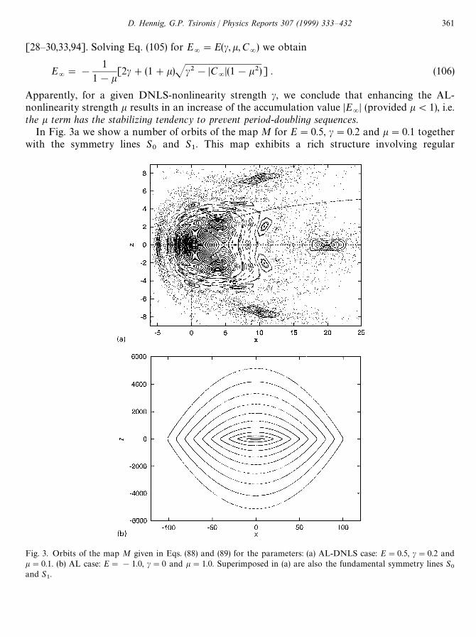
Fig. 3. Orbits of the map M given in Eqs. (88) and (89) for the parameters: (a) AL-DNLS case: E"0.5, c"0.2 andk"0.1. (b) AL case: E"!1.0, c"0 and k"1.0. Superimposed in (a) are also the fundamental symmetry lines S

0and S

1.

[28—30,33,94]. Solving Eq. (105) for E="E(c,k,C

=) we obtain

E="!

11!k

[2c#(1#k)Jc2!DC=D(1!k2) ] . (106)

Apparently, for a given DNLS-nonlinearity strength c, we conclude that enhancing the AL-nonlinearity strength k results in an increase of the accumulation value DE

=D (provided k(1), i.e.

the k term has the stabilizing tendency to prevent period-doubling sequences.In Fig. 3a we show a number of orbits of the map M for E"0.5, c"0.2 and k"0.1 together

with the symmetry lines S0

and S1. This map exhibits a rich structure involving regular


quasiperiodic (KAM) curves which densely fill the large basin of attraction of the stable period-1orbit. The elliptic fixed points of the Poincare—Birkhoff chains of various higher-order periodicorbits are also surrounded by regular KAM curves, while thin chaotic layers develop in the vicinityof the separatrices of the corresponding hyperbolic fixed points. Moreover, outside the structuredcore containing trapped trajectories inside the resonances, a broad chaotic sea has been developedwhere the corresponding unstable orbits may escape to infinity. For comparison we illustrate inFig. 3b the integrable behavior for the AL-map where the corresponding orbits can be generatedfrom Eq. (90).

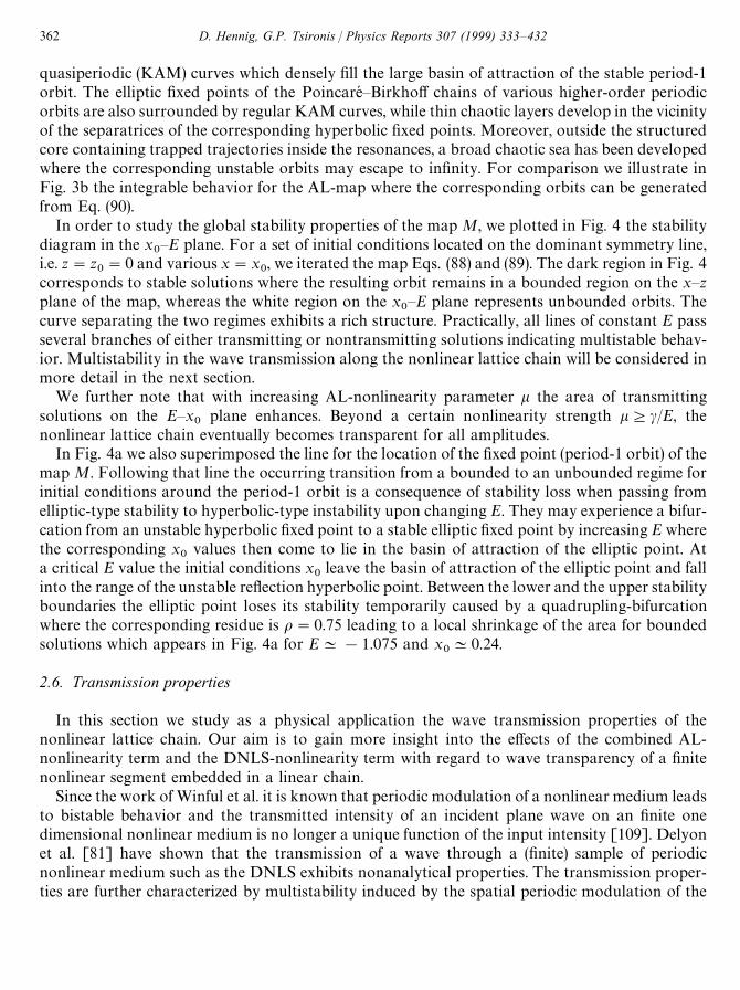
In order to study the global stability properties of the map M, we plotted in Fig. 4 the stabilitydiagram in the x

0—E plane. For a set of initial conditions located on the dominant symmetry line,

i.e. z"z0"0 and various x"x

0, we iterated the map Eqs. (88) and (89). The dark region in Fig. 4

corresponds to stable solutions where the resulting orbit remains in a bounded region on the x—zplane of the map, whereas the white region on the x

0—E plane represents unbounded orbits. The

curve separating the two regimes exhibits a rich structure. Practically, all lines of constant E passseveral branches of either transmitting or nontransmitting solutions indicating multistable behav-ior. Multistability in the wave transmission along the nonlinear lattice chain will be considered inmore detail in the next section.

We further note that with increasing AL-nonlinearity parameter k the area of transmittingsolutions on the E—x

0plane enhances. Beyond a certain nonlinearity strength k5c/E, the

nonlinear lattice chain eventually becomes transparent for all amplitudes.In Fig. 4a we also superimposed the line for the location of the fixed point (period-1 orbit) of the

map M. Following that line the occurring transition from a bounded to an unbounded regime forinitial conditions around the period-1 orbit is a consequence of stability loss when passing fromelliptic-type stability to hyperbolic-type instability upon changing E. They may experience a bifur-cation from an unstable hyperbolic fixed point to a stable elliptic fixed point by increasing E wherethe corresponding x

0values then come to lie in the basin of attraction of the elliptic point. At

a critical E value the initial conditions x0

leave the basin of attraction of the elliptic point and fallinto the range of the unstable reflection hyperbolic point. Between the lower and the upper stabilityboundaries the elliptic point loses its stability temporarily caused by a quadrupling-bifurcationwhere the corresponding residue is o"0.75 leading to a local shrinkage of the area for boundedsolutions which appears in Fig. 4a for EK!1.075 and x

0K0.24.

2.6. Transmission properties

In this section we study as a physical application the wave transmission properties of thenonlinear lattice chain. Our aim is to gain more insight into the effects of the combined AL-nonlinearity term and the DNLS-nonlinearity term with regard to wave transparency of a finitenonlinear segment embedded in a linear chain.

Since the work of Winful et al. it is known that periodic modulation of a nonlinear medium leadsto bistable behavior and the transmitted intensity of an incident plane wave on an finite onedimensional nonlinear medium is no longer a unique function of the input intensity [109]. Delyonet al. [81] have shown that the transmission of a wave through a (finite) sample of periodicnonlinear medium such as the DNLS exhibits nonanalytical properties. The transmission proper-ties are further characterized by multistability induced by the spatial periodic modulation of the


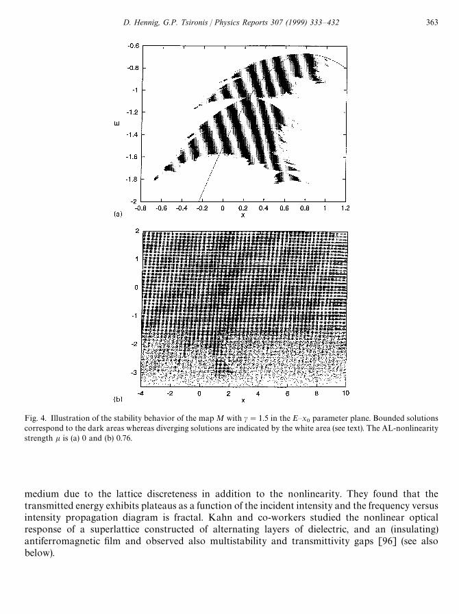
Fig. 4. Illustration of the stability behavior of the map M with c"1.5 in the E—x0

parameter plane. Bounded solutionscorrespond to the dark areas whereas diverging solutions are indicated by the white area (see text). The AL-nonlinearitystrength k is (a) 0 and (b) 0.76.

medium due to the lattice discreteness in addition to the nonlinearity. They found that thetransmitted energy exhibits plateaus as a function of the incident intensity and the frequency versusintensity propagation diagram is fractal. Kahn and co-workers studied the nonlinear opticalresponse of a superlattice constructed of alternating layers of dielectric, and an (insulating)antiferromagnetic film and observed also multistability and transmittivity gaps [96] (see alsobelow).


2.7. Amplitude stability

We study the following transmission problem: Plane waves with momentum k are sentfrom the left towards the nonlinear chain, where they will be scattered into a reflected andtransmitted part:

/n"G

R0exp(ikn)#R exp(!ikn) for 14n4N ,

¹ exp(ikn) for n5N .

We denote by R0, R the amplitudes of the incoming and reflected waves and by ¹ the transmitted

amplitude at the right end of the nonlinear chain. The wave number k is in the interval [!p, p]yielding DED42.

Since the superposition principle is no longer valid in the nonlinear case, the transmittedamplitude ¹ is not uniquely defined by the incident amplitude R

0. To circumvent this difficulty we

solve the inverse transmission problem, i.e. compute the input amplitude R0

for fixed outputamplitude ¹ (see also [81]). The procedure relies on the inverse map given by M~1"M

1MM

1which we interpret as a “backward map” in the following manner: For a given output planewave with transmitted intensity ¹ at the right end of the nonlinear chain we have(/

N`1,/

N)"[¹ exp(ik(N#1)),¹ exp(ikN)]. From the pair (/

N`1, /

N) we obtain (r

N`1, r

N) and

(hN`1

, hN) as well as (x

N`1"2D¹D2cos(k), z

N`1"0). The latter are used as initial conditions for the

map M~1 in the study of the fixed output transmission problem. For a given wavenumber k thecurrent J is fixed through the expression J"D¹D2 sin(k). We see, therefore, that the pair (k, D¹D)initializes the map M~1 completely. Iterating the map M~1 from n"N to n"0 successivelydetermines the amplitudes (r

N~1,2, r

0) and phases (h

N~1,2, h

0) and eventually results in the value

of /0

on the left end of the nonlinear chain.Fig. 5 displays the transmission behavior in the k!D¹D parameter plane (momentum versus

intensity amplitude of an outgoing wave), showing regions of transmitting (white) and nontran-smitting (hatched) behavior. This representation is similar to that used by Delyon et al. and Wanand Soukoulis in the study of the corresponding stationary DNLS-model [81,82].

For a given output wave with intensity D¹D and momentum k the inverse map M~1 has beeniterated by taking a grid of 500 values of k and 250 values D¹D. Correspondingly, to initialize themap M~1 we populate the z-axis with initial conditions x

0"2D¹Dcos(k), z

0"0 and iterate on each

individual point. When the resulting incoming wave intensities DR0D are of the same order of

magnitude as the transmitted intensity, the nonlinear chain is said to be transmitting (white area inFig. 5). In Fig. 5 we show the AL-DNLS case k"0.25, with c"1.

For wave numbers DkD3[p/2,p] the regions of bounded and unbounded solutions are separatedby a sharp smooth curve which can be obtained approximately from the analysis for theinitial wave amplitude stability performed in Section 2.3. Using Eq. (73) the boundary followsfrom

D/TD2"

1kGS1#

2k(1!cos(k))c!2k

!1H , (107)

where /T

is the critical value for the wave amplitude above which stable transmission is necessarilyimpossible.


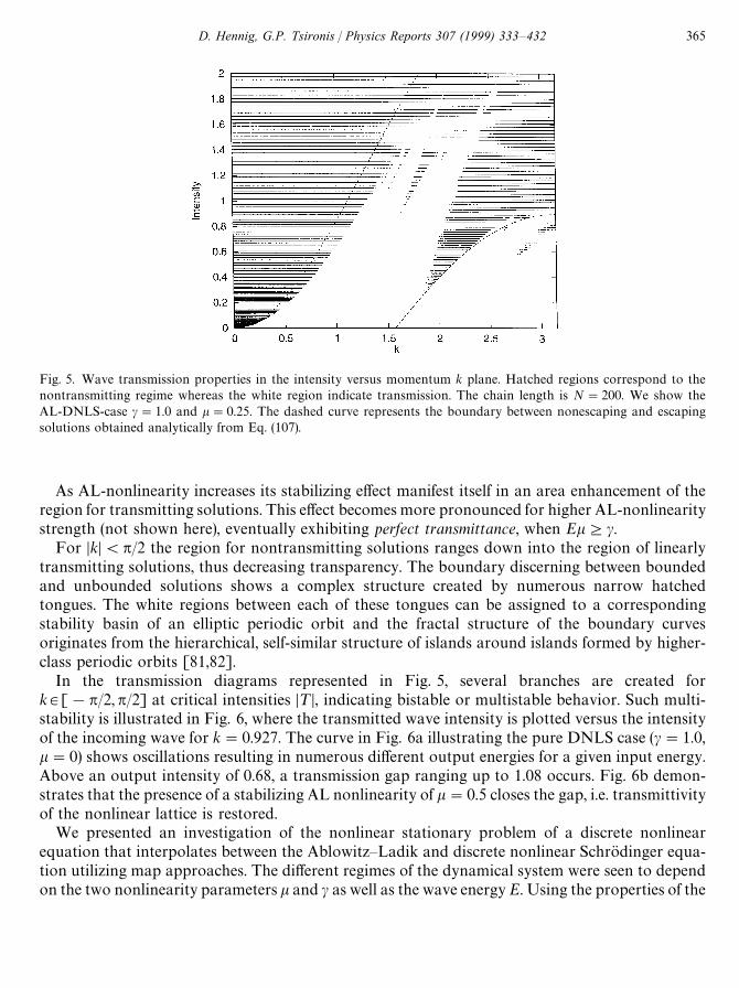
Fig. 5. Wave transmission properties in the intensity versus momentum k plane. Hatched regions correspond to thenontransmitting regime whereas the white region indicate transmission. The chain length is N"200. We show theAL-DNLS-case c"1.0 and k"0.25. The dashed curve represents the boundary between nonescaping and escapingsolutions obtained analytically from Eq. (107).

As AL-nonlinearity increases its stabilizing effect manifest itself in an area enhancement of theregion for transmitting solutions. This effect becomes more pronounced for higher AL-nonlinearitystrength (not shown here), eventually exhibiting perfect transmittance, when Ek5c.

For DkD(p/2 the region for nontransmitting solutions ranges down into the region of linearlytransmitting solutions, thus decreasing transparency. The boundary discerning between boundedand unbounded solutions shows a complex structure created by numerous narrow hatchedtongues. The white regions between each of these tongues can be assigned to a correspondingstability basin of an elliptic periodic orbit and the fractal structure of the boundary curvesoriginates from the hierarchical, self-similar structure of islands around islands formed by higher-class periodic orbits [81,82].

In the transmission diagrams represented in Fig. 5, several branches are created fork3[!p/2,p/2] at critical intensities D¹D, indicating bistable or multistable behavior. Such multi-stability is illustrated in Fig. 6, where the transmitted wave intensity is plotted versus the intensityof the incoming wave for k"0.927. The curve in Fig. 6a illustrating the pure DNLS case (c"1.0,k"0) shows oscillations resulting in numerous different output energies for a given input energy.Above an output intensity of 0.68, a transmission gap ranging up to 1.08 occurs. Fig. 6b demon-strates that the presence of a stabilizing AL nonlinearity of k"0.5 closes the gap, i.e. transmittivityof the nonlinear lattice is restored.

We presented an investigation of the nonlinear stationary problem of a discrete nonlinearequation that interpolates between the Ablowitz—Ladik and discrete nonlinear Schrodinger equa-tion utilizing map approaches. The different regimes of the dynamical system were seen to dependon the two nonlinearity parameters k and c as well as the wave energy E. Using the properties of the


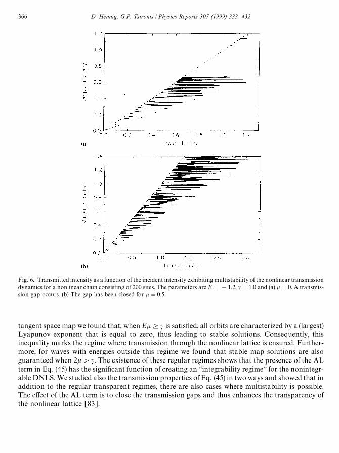
Fig. 6. Transmitted intensity as a function of the incident intensity exhibiting multistability of the nonlinear transmissiondynamics for a nonlinear chain consisting of 200 sites. The parameters are E"!1.2, c"1.0 and (a) k"0. A transmis-sion gap occurs. (b) The gap has been closed for k"0.5.

tangent space map we found that, when Ek5c is satisfied, all orbits are characterized by a (largest)Lyapunov exponent that is equal to zero, thus leading to stable solutions. Consequently, thisinequality marks the regime where transmission through the nonlinear lattice is ensured. Further-more, for waves with energies outside this regime we found that stable map solutions are alsoguaranteed when 2k'c. The existence of these regular regimes shows that the presence of the ALterm in Eq. (45) has the significant function of creating an “integrability regime” for the nonintegr-able DNLS. We studied also the transmission properties of Eq. (45) in two ways and showed that inaddition to the regular transparent regimes, there are also cases where multistability is possible.The effect of the AL term is to close the transmission gaps and thus enhances the transparency ofthe nonlinear lattice [83].


3. Soliton-like solutions of the generalized discrete nonlinear Schrodinger equation

3.1. Introduction

In this chapter we study the localized stationary solutions of the GDNLS equation in the realdomain in greater detail. We show that the results of the stationary analysis can be used to excitelocalized stationary states of designed patterns on the lattice. Stationary localized solutions ofa pure DNLS system were studied in [82,107,108] in the context of wave propagation inperiodically modulated media. In nonlinear optics Kerr type nonlinearities give rise to DNLSequations and the localized solutions are supported by states in the first gap, therefore called gapsolitons [34,95,96,110,112—114]. The corresponding stationary system can be treated by a nonlin-ear map approach. In searching for localized solutions one has to be aware that the stationarynonintegrable DNLS system exhibits irregular chaotic behavior which led the authors of[82,107,108] to the conclusion that perfect localization in a nonintegrable lattice system isimpossible. Nevertheless, we demonstrate that stable localized lattice states conspire with thenonintegrability of the map orbits through homoclinic and heteroclinic connections.

The chapter is organized as follows: In Section 3.2 we introduce the real-valued stationaryAL-DNLS problem and link it with a two-dimensional area-preserving map. We discuss thestability properties of the fixed points of the map. In Section 3.3 we discuss the anti-integrable limitof the GDNLS and prove the existence of localized solutions. In Section 3.4 the Melnikov methodis used to prove the existence of homoclinic orbits thus showing nonintegrability of the map. Withthe help of the Birkhoff normal forms we determine homoclinic orbits analytically in Section 3.5and compute the soliton pinning energy. In order to obtain the heteroclinic orbits we exploita variational approach relating the heteroclinic points to the critical points of a certain actionfunction. In Section 3.6 we excite bright (dark) solitons in the dynamical DNLS using thehomoclinic (heteroclinic) map orbits as initial data. Finally, in Section 3.8 we give a short summary.(Also, see Refs. [99—103,105,106,116].)

3.2. The real-valued stationary problem of the GDN¸S

We investigate the solution properties of the GDNLS where we focus on time-periodic butspatially localized solutions [115]. As is shown below such a study of localized GDNLS statesimplies real-valued stationary amplitudes. Substituting the ansatz

tn(t)"/

nexp(!iut) , (108)

with amplitudes /nand the phase (oscillation frequency) u into Eq. (44), we obtain the following

coupled system for the amplitudes /n:

u/n#c D/

nD2/

n#(»#kD/

nD2)(/

n`1#/

n~1)"0 . (109)

To distinguish the present study (in the real domain) from those performed in the preceding chapter(in the complex domain) we use for the stationary phase the notation u. We further remark that forcomputational convenience the current sign convention for the dispersion term is chosen to beopposite to those of the stationary Eq. (45).


We are particularly interested in solutions exponentially localized at a single site and distinguishtwo situations: (1) D/

nD'D/

n`1D for n'0 and D/

nD(D/

n`1D for n(0 with lim

@n@?=D/

nD"0 corre-

sponding to the bright soliton-like solution, and (2) D/nD(D/

n`1D for n'0 and D/

n`1D(D/

nD for

n(0 with lim@n@?=

D/nD"a'0 resulting in the dark soliton-like solution. Without loss of general-

ity we assume that both types of the soliton-like solutions have their main deviations from thebackground around the central element of the lattice. Furthermore we request for the bright (dark)soliton solution exponential decrease (increase) of the amplitudes apart from the central site forDnDPR.

It can be readily seen that the current J defined by

J"i [/*n/

n~1!/

n/*n~1

] (110)

is conserved for the system of the stationary equations. Since we consider an open lattice chain(without periodic boundary conditions) we can show that localized solutions implies real ampli-tudes /

n3R. To this end we consider the value for the current at one of the ends of the chain

assumed to be of finite length N for the moment. Representing /N~1

by the r.h.s. of thecorresponding stationary equation

»/N~1

"!

u#cD/ND2

»#kD/ND2/N

, (111)

we immediately obtain that J,0. Due to the conservation of J this result must hold for all latticeindices n3[!N,N] which however can only be fulfilled for either the special case of constantamplitudes /

n"constant or, in general, only for real-valued /

n3R. The last result is independent

of the value of N. Hence, for the remainder of this chapter we consider real-valued amplitudes /n.

It is convenient to cast the real-valued second-order difference equation (109) into a two-dimensional map R2PR2 by defining x

n"/

nand y

n"/

n~1where the lattice index plays the role

of discrete “time”. We arrive at the map:

M: Gxn`1

"!

uJ #cJ x2n

1#kJ x2n

xn!y

n,

yn`1

"xn.

(112)

We used the notation uJ "u/» and cJ"c/» and the tildes are conveniently dropped afterwards.Reversibility of the map M is established by the factorization M"M

0M

1with

M0:G

xN "y ,

yN "x ,(113)

M1: G

xN "x ,

yN "!

u#cx2

1#kx2!y ,

(114)

where M0,1

are involutions and their corresponding symmetry lines are given by S0:x"y and

S1: y"!(1/2)(ux#cx3)/(1#kx2). Furthermore, the mapM is an analytic area-preserving map.In order to investigate stationary localized solutions in the form of the bright (dark) soliton,

respectively, it suffices to study the fixed points (period-1 orbits) of the mapM. The fixed points, for


which xL "yL , of this map are located at

xL0"0, xL

B"$J!u#2/c#2k , (115)

where xLB

exists only if sign(u#2)"!sign(c#2k). The stability of the fixed points is governedby their value for the corresponding residues [28,43] o"1/4 [2!Tr(DM(xL ))]. The tangent mapDM is determined by

DM(x)"Au

n!1

1 0 B , (116)

with

un"!

u#(3c!ku)x2n#ckx4

n(1#kx4

n)2

. (117)

The residue corresponding to the fixed point at the origin is

o"14(u#2) . (118)

For u values within the range of the linear band, i.e. DuD(2, 0(o(1 holds and the origin isa stable elliptic fixed point encircled by stable elliptic type map orbits. For DuD'2 (outside therange of the linear band) we distinguish the following two cases:

(i) u(!2, c#2k'0.In this case the residue passes through zero, i.e. o(0, and hence the origin loses stability and is

turned into an unstable hyperbolic point caused by a tangent bifurcation. This hyperbolic point isconnected to itself by a homoclinic orbit created by the (invariant) unstable and stable manifold. Aswill be shown below the homoclinic orbit is manifested on the lattice chain as a soliton-like solutionwhich is equivalent to the so called gap soliton of nonlinear optics lying in the stop band below thelinear passing band [34,112,71].

The pair of points xLB

on the symmetry line S0

form stable elliptic fixed points.

(ii) u'2, c#2k(0.The value for the residue at the origin passes through the value of one, that is o'1, connected

with the onset of a period-doubling bifurcation, where the fixed point is converted into an unstablehyperbolic point with reflection. The newly created period-2 orbits are located on the line x"!y.

The homoclinic map orbit supports on the lattice chain a soliton-like solution which exists in thegap above the linear passing band and has alternating signs for adjacent amplitudes, i.e.sign(/

n`1)"!sign(/

n) as a characteristic feature (see below). This stationary localized structure

has been called a staggered soliton by Cai et al. in their study of the combined AL-DNLS equation[18]. Correspondingly the soliton solution of case (i) is called unstaggered soliton. Note that uponsign change cP!c and uP!u the map has the symmetry property of sign(/

n`1)"!sign(/

n)

so that the unstaggered and staggered soliton replace each other. A third case of unstable fixedpoints can also be attributed to the occurrence of a stationary localized structure on the nonlinearlattice, namely:

(iii) DuD(2 and c#2k(0.Since the frequency is in the linear band the origin is still a stable elliptic fixed point whereas the

pair of fixed points xLB

on the symmetry line S0

represents two unstable hyperbolic fixed points


which are connected to each other via a (pair of) heteroclinic orbits. This heteroclinic map orbitrepresents a kink-like solution, also called a dark soliton. There exist staggered and unstaggeredversions of this soliton, too.

3.3. The anti-integrable limit and localized solutions

In this section we apply the concept of the anti-integrable limit introduced by Aubry andAbramovici [117,118]. We are particularly interested in the impact of the integrable AL term ofEq. (44) on the formation of breathers, i.e. the occurrence of time-periodic, spatially localizedsolutions. Recently, MacKay and Aubry have proven the existence of localized solutions in form ofbreathers for weakly coupled arrays of oscillators [119]. These authors suggested also theapplication of the anti-integrable (or better called no-coupling) limit to prove the existence ofbreather solutions for the DNLS system (cf. Section 9 of Ref. [119]). Using the anti-integrable limitBressloff proved the existence of localized ground states for the standard diffusive Haken modeldescribing a neural network [120]. Due to the formal equivalence of the Haken model toa DNLS-Hamiltonian one can also infer from Bressloff’s result on the existence of (stationary)breathers for the DNLS. However, the present study involves besides the nonintegrable DNLSterm also additionally the integrable AL contribution. It is worth mentioning that the AL systemby itself has no anti-integrable limit.

The spatial behavior of the breathers tn(t)"exp(!iut)/

nof the GDNLS is described by

a stationary equation with real amplitudes /n3R [119] (see also discussion above). Since

Dtn(t)D2"/2

ndoes not change with time these solutions can be viewed as static breathers. The action

for the real-valued AL-DNLS system reads

F"+nG!

12kAu!

ckBln(1#k/2

n)!

c2k

/2n#

»

2(/

n`1!/

n)2H . (119)

(We shifted the linear band by 2».) The map orbits are determined by

»(/n`1

#/n~1

!2/n)"!

u#c/2n

1#k/2n

/n. (120)

The anti-integrable limit for the AL-DNLS system is obtained for vanishing hopping parameter»"0, where the action is represented as the sum over local on-site potentials º(/

n):

FAI"!+

nG

12kAu!

ckBln(1#k/2

n)#

c2k

/2nH (121)

,+n

º(/n) . (122)

The orbits for the stationary problem are determined by

º(/n)

/n

,º@(/n)"0 , (123)

yielding the rest positions

/I0"0, /I

B"$J!u/c, u(0, c'0 . (124)


Since orbit points at sites n#1 and n are mutually independent of each other an orbit can beassociated with an arbitrary sequence of three symbols assigned to (/I

0, /I

B). Hence, the orbits

are trivially equivalent to a Bernoulli shift establishing the existence of chaotic orbits [117,118]. Wecan prove that some chaotic solutions of the anti-integrable limit persist, at least up to a criticalvalue »

#3*5.

Theorem. For

»#3*5

4

Dº@(DuB

D)D4/

.!9

(125)

there exists a unique solution of Eq. (120) such that for all n deviations from the rest position /I0

arebounded by

D/nD4u

`, (126)

and deviations from /IB

lie in the range given by

/.*/

4D/nD4/

.!9, (127)

with

uB"$G

12cCAu!3

ckB#Su2#A3

ckB

2!10u

ckDH

1@2, (128)

/.*/

"G12cC8»#3*5

#u!3ck#SA3

ck!u!8»

#3*5B2#16c»

#3*5!4cuDH

1@2(129)

and /.!9

is the maximum positive root of the equation

º(/n)"º(u

`) . (130)

Proof. Eq. (120) can be rewritten as

»(/n`1

#/n~1

!2/n)"º@(/

n) . (131)

From Eq. (127) we obtain that

supn

D/n`1

#/n~1

!2/nD44/

.!9, (132)

which yields

4»/.!9

5Dº@(/n)D . (133)

When

»#3*5

(

maxnDº@(/

n)D

4/.!9

"

Dº@(DuB

D)D4/

.!9

, (134)

then Eq. (120) has infinitely many solutions. But, in each interval given by the inequalities (126) and(127), there is one and only one solution and hence, the problem is uniquely defined.


From the graph of ºA(/n) it can be readily seen that ºA(/

n)'0 in the interval given by Eq. (126).

Further, when (127) holds then ºA(/n)(!4». The Jacobian operator D2F is tridiagonal with

diagonal elements ºA#2» and off-diagonal elements !». Since DºA#2»D'2», the operatorD2F is invertible and its inverse is bounded. Hence it follows from the implicit function theoremthat an orbit has a locally unique continuation for »(»

#3*5[117—123]. h

It can easily be shown that »#3*5

/k(0 and /.!9

/k(0. From this we note that the presenceof the integrable AL-term has a destabilizing influence on the continuation process of the solutionsof the anti-integrable limit in the sense that, the higher the k-values are the lower become the»-values to which the continuation can be carried out. Moreover, the possible maximal amplitudes/.!9

of the continued solutions decrease with increasing k. An interesting case arises when in theno-couling limit »"0 only one site is excited while all the others remain unexcited (e.g. /

0"/I

`and /

nE0"0). This results in a so called one-site breather which is maintained under the action of

the coupling 0(»(»#3*5

and its spatially exponential localization can be proven with the help ofTheorem 3 of [119].

3.4. The Melnikov function and homoclinic orbits

As is well known in generic nonintegrable maps the stable and unstable manifolds of hyperbolicequilibria cross each other in homoclinic points; or there might appear crossings of the stable andthe unstable manifolds of different hyperbolic points, called heteroclinic connections. Such two-dimensional maps are often associated with the Poincare map of periodically perturbed two-dimensional flows [28]. For these time-continuous flows the Melnikov function proved to bea powerful method to show the existence of orbits homoclinic to a hyperbolic equilibrium. Glasseret al. [124] extended the Melnikov analysis to two-dimensional discrete maps of the plane whichare of the form u

n`1"F(u

n)#eG(u

n) with u"(x, y)3R2. Thus the r.h.s. is assumed to consist of

a completely integrable part F and a small nonintegrable perturbation eG with e;1. Furthermore,the unperturbed system of e"0 possesses an unstable equilibrium characterized by coincidingstable and unstable manifolds forming a perfect unperturbed separatrix on which the solution isknown explicitly. Based on geometric arguments a Melnikov function was developed in [124]measuring the distance between the stable and unstable manifolds under the action of theperturbation.

For a perturbational treatment we consider the nonlinear term related with c as a small(nonintegrable) perturbation of the integrable AL map (c"0, kO0). Therefore we introduce inEq. (112) the small parameter e:

xn`1

"!

u#ecx2n

1#kx2n

!yn,

yn`1

"xn,

(135)

whose integrable part (e"0) possesses a separatrix given by

kx2y2#x2#y2#uxy"0 . (136)


In the first quadrant the separatrix loop can be parameterized by

xn(t)"

1

Jksinhb sech(t!nb) , (137)

yn(t)"

1

Jksinhb sech(t!(n#1)b) , (138)

where cosh b"!u/2 and t is a real parameter regulating the position on the separatrix loop.Note that the AL soliton center of x

0(0)"J(u2/4!1)/k and y

0(0)"!2x

0(0)/u is determined on

the map plane by the intersection point of the AL separatrix loop with the symmetry line S1.

According to [124] the Melnikov function is given by

M(t;u,k, c)"DDu0(t)DDD@(0) , (139)

with

D@(0)"=+

k/~=

G(xk~1

, yk~1

)'vk, (140)

where the wedge product is (u1, u

2)'(v

1, v

2)"u

1v2!u

2v1. Therefore the unit tangent vector to the

separatrix is given as

vk(t)"u

k(t)/DDu

0(t)DD , (141)

where

uk(t)"A!y

k!

u2xk!kx2

kyk, x

k#

u2yk#kx

ky2kB . (142)

In our case the perturbation is G(xn)"(!ecx3

n/(1#kx2

n), 0). Thus we have

D@(0)"!ec=+

k/~=

x3k~1

1#kx2k~1Cxk

#

u2xk~1

#kxkx2k~1D

"

ecu

=+

k/~=

(xk`1

#xk~1

)x2kCxk`1

#

u2xk#kx

k`1x2kD

"

ecu

=+

k/~=

[x2kx2k`1

#ux3kxk`1

#kx4kx2k`1

#x4k`1

] . (143)

We therefore need to calculate sums of the form S1(a, b, j)"+=

k/~=sech2(jn!a) sech2(jn!b).

Using the Poisson summation formula we have

S1(a, b, j)"

=+

k/~=P

=

~=

exp(2pinx) sech2(jx!a) sech2(jx!b) dx . (144)


The integral is evaluated using residue calculus:

P=

~=

exp(ax) sech2(jx!a) sech2(jx!b) dx

"!

pj

cosechAap2jBcosech2 dC

ajAexpC!

aaj D#expC!

abj DB

#C2 coth dAexpC!aaj D!expC!

abj DBD , (145)

where d"a!b. Setting a"!2pin and performing the remaining sum we get

S1(a, b, j)"

2pj

[h(d)II (a, b, j)#f (d)I(a, b, j)] , (146)

with

I"/Apbj

,p2

j B!/Apaj

,p2

j B#dp

, (147)

II"!

/b

!

/a

!

2p

, (148)

where

/(x, u)"=+n/1

sin(2nu) cosech(nx)"Kp

[E(am(2Ku/p))!2uE/p] (149)

and finally h(d)"cosech2 d and f (d)"2 cosechd coth d. Similarly, we have

S(a, b, j)"=+

k/~=

sech(jn!a) sech(jn!b)"g(d)I(a, b, j) , (150)

where g(d)"cosech d. The sum S2(a, b, j)"+=

k/~=sech3(jn!a) sech(jn!b) follows from

S2"(S!SA)/2, where the primes denote derivatives with respect to a. The sum

S3(a, b, j)"+=

k/~=sech4(jn!a) sech2(jn!b) can be constructed as S

3"2

3S1!1

6SA1

while the lastsum +=

k/~=sech4(jn!a) is S

2(a,a, j). Thus we obtain

D@(0)"ecuk

sinh4b(S1(t, t!b, b)!2 cosh bS

2(t, t!b, b)

# sinh2bS3(t, t!b, b)#S

2(t, t,b)) (151)

which reduces to

D@(0)"!

ecuk

sinh4 bA4 cothbAK3k2

b2 BdnC2Ktb DsnC

2Ktb DcnC

2Ktb D

#

83

K4k2

b3 Adn2C2Ktb Dcn2C

2Ktb D!dn2C

2Ktb Dsn2C

2Ktb Dk2sn2C

2Ktb Dcn2C

2Ktb DBB ,

(152)


where E(k)/K(k)"p/b, K and E being the complete elliptic integral of the second kind andthe associated complete elliptic integral of the second kind, respectively. Eq. (152) shows thatthe Melnikov function is a periodic function of t with an infinite number of simple zeros proving thepresence of homoclinic chaos in the perturbed map. As a result of the nonintegrability the stableand unstable manifolds of the hyperbolic fixed points of the perturbed map are no longer identical,but intersect and create a homoclinic tangle. Eq. (152) also shows that the separatrix splitting isproportional to the ratio c/(uk). The same ratio was found in [83] to limit the parameter regionwhere the map (112) shows regular motion. Finally, from Eq. (152) it is obtained that the distancebetween successive transversal intersections of the stable and unstable manifolds purely depends onthe ratio K/b, which in turn only depends on u and not directly on the nonlinearity parametersc and k. The nonlinearity parameters appear only in front of the Melnikov function (153) as a factorregulating the degree of the separatrix splitting. Apparently with higher nonintegrability parameterc the splitting grows whereas the integrability parameter k acts in the opposite direction, namelysuppresses the splitting.

According to the defining relation between k and u we can obtain that k has a rather slowdependence on u which means that k can be considered small even for rather large u such that it isreasonable consider k as small in Eq. (152). This approximation reduces the complexity of D@(0)considerably. Using small k expansions of the Jacobian Elliptic functions [125]

D@(0)"!

eck

A(u) cosA4Kb

t#hB#O(k2) , (153)

where

A(u)"2K3k2

ub2 Scoth2b#26K2

9b2sinh4b, tan h"

3b cothb4K

. (154)

The distance between successive zeros of the Melnikov function is given by

Dt"pb4K

K

12lnA!

u2#S

u2

4!1B,

12

ln(j) , (155)

telling us that the distance between two adjacent intersections of the stable and unstable manifolddepends solely on the oscillation frequency u. The distance vanishes at the band edge of u"!2and grows logarithmically when u ranges further down in the gap. Interestingly, the quantity j inEq. (155) is identical to the maximal eigenvalue of the linearized map around the hyperbolic pointat the origin.

3.5. Normal form computation of the homoclinic tangle

In this section we use the Birkhoff normal forms to compute the homoclinic orbit correspondingto the unstable hyperbolic point at the map origin for u(!2 and c#2k'0. The Birkhoffnormal form of an area-preserving map yields a simplified version of the map achieved bya canonical transformation in form of a formal series expansion [126]. Normal forms are powerfultools for analytical determination of homoclinic orbits of two-dimensional maps. Recently Tabac-man [127] developed another method for computing homoclinic and heteroclinic orbits relying on


an action principle. In a subsequent section we exploit this method to obtain the orbit heteroclinicto the fixed points (xL

B,yL

B). Later we need the “exact” location of the intersection points of the

stable and unstable manifolds to use them as initial data in order to excite stationary localizedstates of the GDNLS.

We begin by rewriting the map of Eq. (112) as follows:

M: GxN "!ux!u

(c/u!k)x2

1#kx2x!y ,

yN "x .(156)

The linear part

xN "!ux!y, yN "x (157)

is diagonalized through the canonical transformation

P"j`x!y, Q"j~x!y , (158)

and

jB"12[!u$Ju2!] (159)

are the eigenvalues of the linear transformation (157). The inverse transformation is given by

x"P!Q

j`!j~, y"

j~P!j`Qj`!j~

. (160)

After a scaling PPJkP and QPJkQ and with the help of j,j`"1/j~ we obtain for thetransformed map:

PM "jP!Ack!uB

j4

(j2!1)3(P!Q)3

11#1/(j!1/j)2(P!Q)2

, (161)

QM "1jQ!A

ck!uB

j2

(j2!1)3(P!Q)3

11#1/(j!1/j)2(P!Q)2

, (162)

or its equivalent Taylor expansion about the origin

PM "jP#Ack!uBj

=+n/1

(!1)nCj

(j2!1)(P!Q)D

(2n`1), (163)

QM "1jQ#A

ck!uB

1j

=+n/1

(!1)nCj

(j2!1)(P!Q)D

(2n`1). (164)

Birkhoff [126] introduced a canonical transformation based on the series expansion

P"m#=+k/2

k+l/0

pkl

mk~lgl , (165)

Q"g#=+k/2

k+l/0

qkl

mk~lgl , (166)


such that the (m, g) map is given by

mM "º(mg)m , (167)

gN "[º(mg)]~1g . (168)

The function º depends only on the product mg and has a formal series expansion

º(mg)"jA1#=+k/1

º2k

(mg)kB . (169)

Moser [128] proved the convergence of the series (167)—(169) in a disc surrounding the originprovided the series in Eqs. (163) and (164) represent analytical functions which is true in our case.Moreover, it was shown, that whenever the inverse map is also analytic, the region of convergenceof the series can be extended in narrow strips along the stable and unstable manifolds, respectively[129]. Furuya and Ozorio de Almeida [130] used the Birkhoff normal form for a precisecomputation of homoclinic points of the standard map and our approach proceeds along the samelines for the AL-DNLS map.

It is useful to define the auxiliary series

(P!Q)2n`1" +k/2n`1

(d2n`1)klmk~lgl . (170)

The recursion relations for the expansion coefficients are then determined by

jºk~1

dk,2l`1

!jpkl"A

ck!uBj

(k~1)@2+n/1

(!1)n(d2n`1)klA

jj2!1B

2n`1

!jk~2l +n/0

pk~2n,l~n

(ºk~2l)2n

, (171)

j(º~1)k~1

dk,2l~1

!

1jqkl"A

ck!uB

1j

(k~1)@2+n/1

(!1)n(d2n`1)klA

jj2!1B

2n`1

!jk~2l +n/0

qk~2n,l~n

(ºk~2l)2n

. (172)

The stable and unstable manifold of the map M are the images of the g"0 and the m"0 axesunder the transformation º. Since the Melnikov function possesses infinitely many simple zerosthe stable and unstable manifold cross each other in homoclinic points which we can compute fromthe images of the two axes under º. This method provides the homoclinic orbit with uniformprecision. The unstable manifold as the projection on the m axis is determined by the odd-powerseries

P"m#=+k/3

pk0

mk, Q"

=+k/3

qk0

mk (173)


for which the coefficients pk0

and qk0

can be given in closed form

pk0"A

ck!uBj

1jk!j

(k~1)@2+n/1

(!1)nAj

j2!1B2n`1

(d2n`1)k0

KAck!uBj

1jk!j

(!1)(k~1)@2Aj2

j2!1Bk, (174)

qk0"A

ck!uB

1j

1jk!1/j

(k~1)@2+n/1

(!1)nAj

j2!1B2n`1

(d2n`1)k0

KAck!uB

1j

1jk!1/j

(!1)(k~1)@2Aj2

j2!1Bk. (175)

We have omitted terms of order higher than j~2. Inserting Eqs. (174) and (175) into Eq. (173) weobtain

P"m#Ack!uBj

=+k/3

1jk!j

(!1)(k~1)@2Aj2

j2!1Bkmk . (176)

If again terms of the order higher than j~2 are dropped the series can be summed up yielding

P"m!Ack!uB

m1#(m/j)2A

mjB

2. (177)

Correspondingly, we obtain

Q"Ack!uB

1j

=+k/3

1jk!(1/j)

(!1)(k~1)@2Aj2

j2!1Bkmk , (178)

"!Ack!uB

m3

j4

m1#(m/j)2

#O(j~2) . (179)

Using the inverse transformation of Eq. (160) the unstable manifold is determined by

x"jyG1#(c!uk)A1!1j2B

3 y2

j2#(j2!1)2kyH . (180)

Apparently there is no intersection for c"uk for which the map degenerates to a linear one. Sincethe map orbits obey the symmetry x%y the stable manifold is obtained from Eq. (180) byexchanging x and y.

3.6. Homoclinic, heteroclinic orbits and excitations of localized solutions

We have seen in Section 3.2 that in the map-plane the origin (xn,y

n),(/

n`1,/

n)"(0, 0) forms

a hyperbolic fixed point p as long as DuD'2 which possesses its invariant stable and unstablemanifolds. Points belonging to the stable manifold W4(p) approach the fixed point p under mapiteration Mn for nPR, likewise points on the unstable manifold W6(p) reach the fixed point pfor nP!R. Thus going along the invariant manifolds of the hyperbolic fixed point localized


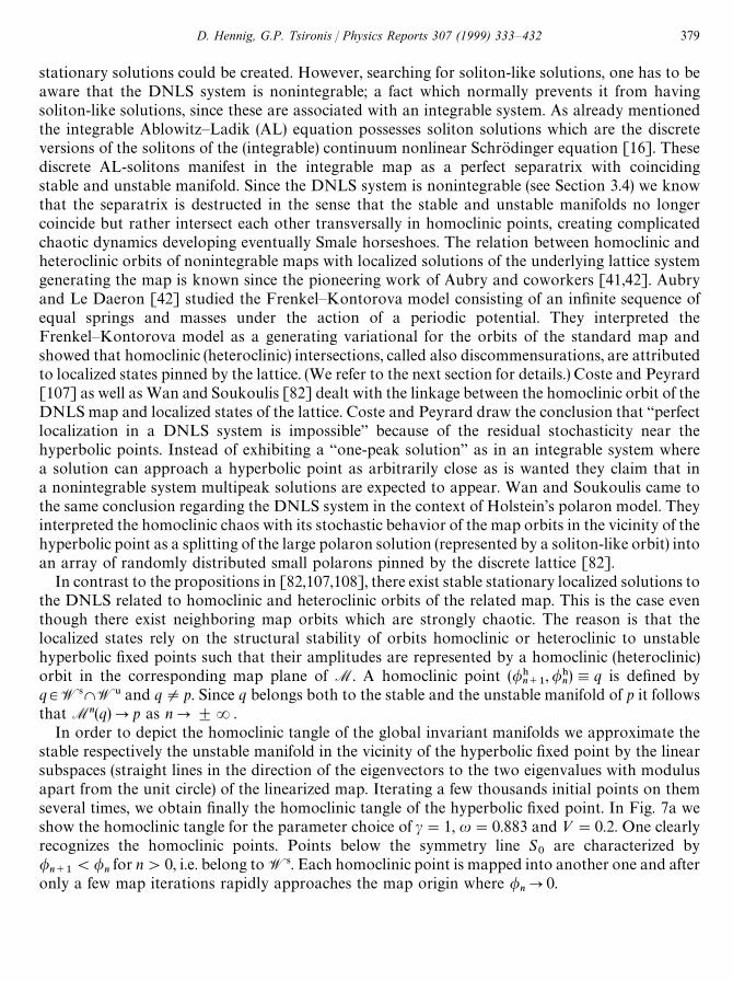
stationary solutions could be created. However, searching for soliton-like solutions, one has to beaware that the DNLS system is nonintegrable; a fact which normally prevents it from havingsoliton-like solutions, since these are associated with an integrable system. As already mentionedthe integrable Ablowitz—Ladik (AL) equation possesses soliton solutions which are the discreteversions of the solitons of the (integrable) continuum nonlinear Schrodinger equation [16]. Thesediscrete AL-solitons manifest in the integrable map as a perfect separatrix with coincidingstable and unstable manifold. Since the DNLS system is nonintegrable (see Section 3.4) we knowthat the separatrix is destructed in the sense that the stable and unstable manifolds no longercoincide but rather intersect each other transversally in homoclinic points, creating complicatedchaotic dynamics developing eventually Smale horseshoes. The relation between homoclinic andheteroclinic orbits of nonintegrable maps with localized solutions of the underlying lattice systemgenerating the map is known since the pioneering work of Aubry and coworkers [41,42]. Aubryand Le Daeron [42] studied the Frenkel—Kontorova model consisting of an infinite sequence ofequal springs and masses under the action of a periodic potential. They interpreted theFrenkel—Kontorova model as a generating variational for the orbits of the standard map andshowed that homoclinic (heteroclinic) intersections, called also discommensurations, are attributedto localized states pinned by the lattice. (We refer to the next section for details.) Coste and Peyrard[107] as well as Wan and Soukoulis [82] dealt with the linkage between the homoclinic orbit of theDNLS map and localized states of the lattice. Coste and Peyrard draw the conclusion that “perfectlocalization in a DNLS system is impossible” because of the residual stochasticity near thehyperbolic points. Instead of exhibiting a “one-peak solution” as in an integrable system wherea solution can approach a hyperbolic point as arbitrarily close as is wanted they claim that ina nonintegrable system multipeak solutions are expected to appear. Wan and Soukoulis came tothe same conclusion regarding the DNLS system in the context of Holstein’s polaron model. Theyinterpreted the homoclinic chaos with its stochastic behavior of the map orbits in the vicinity of thehyperbolic point as a splitting of the large polaron solution (represented by a soliton-like orbit) intoan array of randomly distributed small polarons pinned by the discrete lattice [82].

In contrast to the propositions in [82,107,108], there exist stable stationary localized solutions tothe DNLS related to homoclinic and heteroclinic orbits of the related map. This is the case eventhough there exist neighboring map orbits which are strongly chaotic. The reason is that thelocalized states rely on the structural stability of orbits homoclinic or heteroclinic to unstablehyperbolic fixed points such that their amplitudes are represented by a homoclinic (heteroclinic)orbit in the corresponding map plane of M. A homoclinic point (/)

n`1, /)

n),q is defined by

q3W4WW6 and qOp. Since q belongs both to the stable and the unstable manifold of p it followsthat Mn(q)Pp as nP$R.

In order to depict the homoclinic tangle of the global invariant manifolds we approximate thestable respectively the unstable manifold in the vicinity of the hyperbolic fixed point by the linearsubspaces (straight lines in the direction of the eigenvectors to the two eigenvalues with modulusapart from the unit circle) of the linearized map. Iterating a few thousands initial points on themseveral times, we obtain finally the homoclinic tangle of the hyperbolic fixed point. In Fig. 7a weshow the homoclinic tangle for the parameter choice of c"1, u"0.883 and »"0.2. One clearlyrecognizes the homoclinic points. Points below the symmetry line S

0are characterized by

/n`1

(/nfor n'0, i.e. belong to W4. Each homoclinic point is mapped into another one and after

only a few map iterations rapidly approaches the map origin where /nP0.


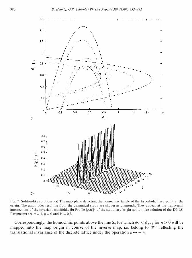
Fig. 7. Soliton-like solutions. (a) The map plane depicting the homoclinic tangle of the hyperbolic fixed point at theorigin. The amplitudes resulting from the dynamical study are shown as diamonds. They appear at the transversalintersections of the invariant manifolds. (b) Profile Dt

n(t)D2 of the stationary bright soliton-like solution of the DNLS.

Parameters are: c"1, k"0 and »"0.2.

Correspondingly, the homoclinic points above the line S0

for which /n(/

n`1for n'0 will be

mapped into the map origin in course of the inverse map, i.e. belong to W6 reflecting thetranslational invariance of the discrete lattice under the operation n%!n.


Let us now use our knowledge about the homoclinic (heteroclinic) orbits to initiate (stationary)localized solutions for the time-dependent DNLS dynamics. In order to invoke the homoclinic maporbit as an initial condition for the dynamics, a sufficiently accurate location of the orbit members(homoclinic intersection points) is demanded. Obviously, the corresponding amplitudes could beread off from the map plane as the coordinates of the homoclinic intersections. However, this maynot be accurate enough to ensure that the spatial behavior of the amplitudes of correspondingdynamical trajectory t

n(t)"/

nexp(!iut) follows the homoclinic orbit /)

nclosely enough, thus

representing a nonlinear eigenstate. Therefore we use the normal form of Eqs. (176) and (178) tocompute the homoclinic orbit “exactly”.

For a study of the dynamics of soliton-like solutions for the DNLS given in Eq. (44) we usea lattice of chain length N"201. We implement the analytically computed homoclinic orbit/)n

with n3[!N/2, N/2] as initial conditions Re tn(t"0)"/

nand Imt

n(t"0)"0. The result

for the soliton-like solution is illustrated in Fig. 7b. Using a Fast-Fourier-Transform-routine wedetermined the oscillation frequency to u"0.879$0.004, which is in fairly good agreement withthe value for frequency put in the map, i.e. u"0.883. We inserted the (dynamical) amplitudesDt

n(t)D2 as diamonds on the map plane in Fig. 7a to show that they coincide with the homoclinic

orbit. The stationary localized soliton-like solution has the following amplitude pattern(2,C,C,C,2) where the dots stand for vanishingly small amplitudes. This localized mode iscentered at a single site. Aceves et al. showed also that these excitation pattern of DNLS results instable steady-state solutions [77—79].

In the same manner we proceed with the kink-like (dark soliton) solution for values of u insidethe linear band. To derive the heteroclinic orbit with high precision we apply a variationalapproach developed recently by Tabacman [127] to compute homoclinic and heteroclinic orbitsfor twist maps. The advantage of this method is that it only requires knowledge of the generatingfunction of the map and a local approximation of the stable and unstable manifolds of orbits nearthe fixed points. The approximate manifolds can be obtained with the help of the linear subspacesof the tangent map taken at the fixed point at the origin as described above. Equipped with theseapproximate invariant manifolds, there remains to find the critical point of a certain function¼

Nwhich is related to the generating function of the map (see Proposition 7 in [127]). The map

can be rewritten in terms of the variables qn"/

nand p

n"q

n!q

n~1. The corresponding map

orbits can be derived from the generating function

S(qn, q

n`1)"1

2(q

n`1!q

n)2#(1/2k)(c/k!u)ln(1#kq2

n)!(c/2k#1) ,

with the relations pn"!S(q

n, q

n`1)/q

nand p

n`1"S(q

n, q

n`1)/q

n`1. One can define an action

function ¼N

the critical points of which delivers the orbit heteroclinic to the fixed points at(qL

~"xL

~, pL

~"0) and (qL

`"xL

`, pL

`"0). The action function ¼

Nis then given by

¼N(q

0,2, q

N)"U6(q

0)#

N+n/0

S(qn, q

n`1)!U4(q

N) ,

where the functions U6(q0) and U4(q

N) describe locally the stable and unstable manifolds W6(qL

~, pL )

and W4(qL`

, pL ), respectively. These functions U4,6 can be computed using the linear subspaces at thefixed points. To compute the critical values of the function ¼

Nwe used a Newton method.

Apparently it is sufficient to obtain one single member of the heteroclinic orbit and then to use themap for getting the others as iterates. When iterating along the stable manifold we approach soon


(typically after 5—8 numbers of iteration) the close vicinity of the hyperbolic fixed points where theorbit stays. Alternatively, one can also use normal form computations in order to generate theheteroclinic orbit. However, for heteroclinic orbits more than one normal form has to be evaluated.

Fig. 8a shows the map plane for the kink-like solution. Again we have inserted the kinkamplitudes Dt

n(t)D2 along the lattice as diamonds in the map plane shown in Fig. 8a.

In this way excitation of the staggered solitons is also possible. Note that staggered localizedDNLS modes have been observed experimentally in a real electrical network [23].

The map for the stationary solutions enables one also to predict the existence of another kind ofstationary localized solution with amplitude pattern of the form (2,C,C,C,C,2), i.e. it is supportedby a homoclinic orbit having the turnstile as one homoclinic point located on the symmetry liney"x, i.e. /

n`1"/

n. This localized mode is centered between two lattice sites. Its energy is higher

than that of the above mentioned localized mode centered at one single lattice site (see also nextsection).

We close this section with the remark that the complete dynamical DNLS system is studied inRef. [132]. It was found that the odd-parity mode is in fact a stable localized standing excitation ofDNLS sustaining symmetry breaking perturbations of its mode pattern. Recently Aceves et al. alsoshowed that the preferred stable localized DNLS states are supported by states having exponenti-ally decaying amplitudes around the maximal amplitude at a single-site, i.e. the odd parity mode.On the other hand, the even-parity mode exhibits a dynamical instability and collapses to theodd-parity mode under the impact of symmetry breaking perturbations. These results are inagreement with the findings in [104].

3.7. The soliton pinning energy

As a consequence of the nonintegrability of the map M and the resulting transversal intersectionof the stable and unstable manifolds the soliton-like solutions are pinned, i.e. they cannot betranslated over the lattice from one point to an adjacent without overcoming an energetic barrier[118]. The pinning energy can be computed with the help of the normal forms as done in [130] forthe solitons of the standard map. We use here another approach based on the findings of theMelnikov function. Kivshar and Campbell [133] studied the pinning energy (Peierls—Nabarropotential barrier) for the localized modes of the DNLS system, i.e. for cO0 and k"0.

There exist two homoclinic orbits whose points alternate along the invariant manifolds. Each ofthe homoclinic orbits has one of its points on the symmetry line S

0and S

1, respectively. These

points rapidly approach the map plane origin under the mapping where they stay most of the time.The homoclinic orbit crossing S

0which we denote by MU

%7%/N represents an excitation pattern of

(2CCCC2) on the lattice chain. Such a stationary excitation pattern was called even-parity modein [98] and sometimes also inter-site centered local mode [104]. The other homoclinic orbit MU

0$$N

possesses three large amplitudes (/~1

, /0, /

1) and has the mode pattern (2CCC2) which was

called the odd-parity mode [97] or on-site centered local mode [104]. The point (/~1

, /0) is

located on S1. For positive (negative) c#2k the unstaggered odd-parity (staggered even-parity)

mode has lower action (energy) than the unstaggered even-parity (staggered odd-parity) mode. Tosee this for c#2k'0, one starts iterating the map M at the turnstile of x.!9

%7%/"y.!9

%7%/, (a member of

the unstaggered even-parity mode), and goes along the stable manifold in the range of y'x till thenext intersection point is met. Then one follows the unstable manifold back to the turnstile. In this


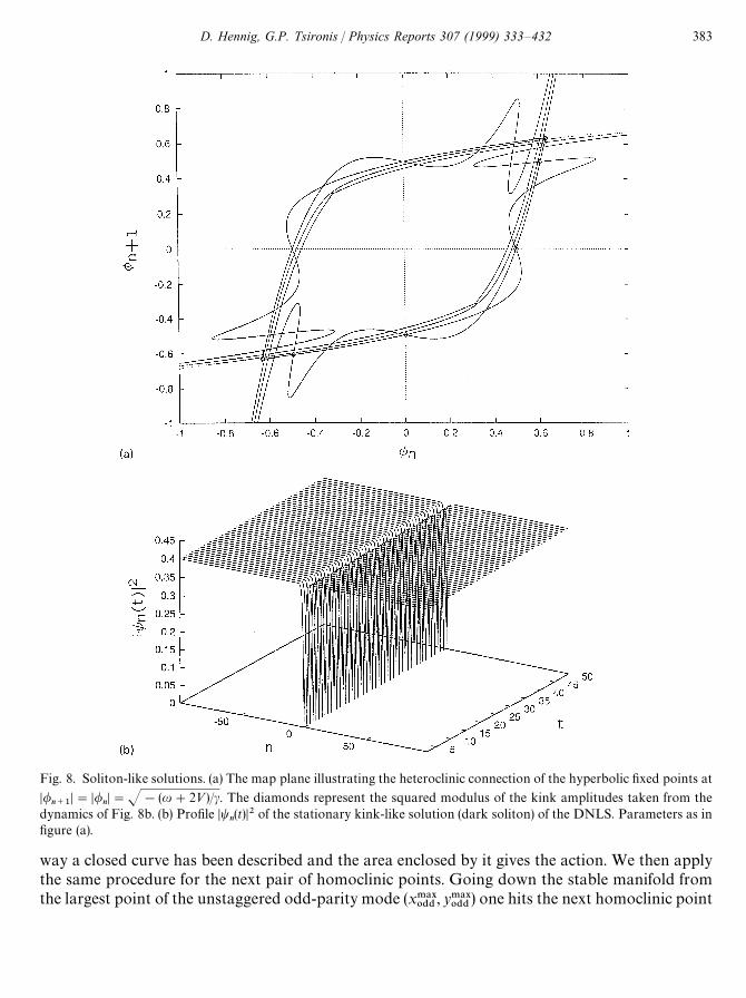
Fig. 8. Soliton-like solutions. (a) The map plane illustrating the heteroclinic connection of the hyperbolic fixed points at

D/n`1

D"D/nD"J!(u#2»)/c. The diamonds represent the squared modulus of the kink amplitudes taken from the

dynamics of Fig. 8b. (b) Profile Dtn(t)D2 of the stationary kink-like solution (dark soliton) of the DNLS. Parameters as in

figure (a).

way a closed curve has been described and the area enclosed by it gives the action. We then applythe same procedure for the next pair of homoclinic points. Going down the stable manifold fromthe largest point of the unstaggered odd-parity mode (x.!9

0$$, y.!9

0$$) one hits the next homoclinic point


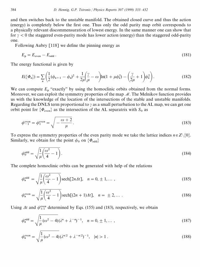
and then switches back to the unstable manifold. The obtained closed curve and thus the action(energy) is completely below the first one. Thus only the odd parity map orbit corresponds toa physically relevant discommensuration of lowest energy. In the same manner one can show thatfor c(0 the staggered even-parity mode has lower action (energy) than the staggered odd-parityone.

Following Aubry [118] we define the pinning energy as

E1"E

%7%/!E

0$$. (181)

The energy functional is given by

E(MUnN)"+

nA12

(/n`1

!/n)2#

12kA

ck!uBln(1#k/2

n)!A

c2k

#1B/2nB . (182)

We can compute E1

“exactly” by using the homoclinic orbits obtained from the normal forms.Moreover, we can exploit the symmetry properties of the map M. The Melnikov function providesus with the knowledge of the location of the intersections of the stable and unstable manifolds.Regarding the DNLS term proportional to c as a small perturbation to the AL map, we can get oneorbit point for MU

%7%/N as the intersection of the AL separatrix with S

0as

/%7%/~1

"/%7%/1

"S!

u#2k

. (183)

To express the symmetry properties of the even parity mode we take the lattice indices n3ZCM0N.Similarly, we obtain for the point /

0on MU

0$$N

/0$$0

"S1kA

u2

4!1B . (184)

The complete homoclinic orbits can be generated with help of the relations

/0$$n

"S1kA

u2

4!1B sech[2nDt], n"0,$1,2 , (185)

/%7%/n

"S1kA

u2

4!1B sech[(2n#1)Dt], n"$2,2 . (186)

Using Dt and /%7%/B1

determined by Eqs. (155) and (183), respectively, we obtain

/0$$n

"S1k

(u2!4) (jn#j~n)~1, n"0,$1,2 , (187)

/%7%/n

"S1k

(u2!4) (jn@2#j~n@2)~1, DnD'1 . (188)


Taking the respective excitation patterns into account, we derive for the soliton energies

E0$$

"

1k

[u2!4]N+n/0CA

1jn`1#j~(n`1)

!

1jn#j~nB

2!A

ck#2B

1jn#j~nD

#

1kA

ck!uB

N+n/0

lnA1#[u2!4]1

jn#j~nB#O(j~2(N`2)) , (189)

and

E%7%/

"!

1k

Ju#2 AJ2!u1

j#j~1!1B

2

#

1kA

ck!uB ln(1#k(/%7%/

1)2)!A

ck#2B (/%7%/

1)2

#

1k

[u2!4]2(N`1)

+n/0

CA1

j(n`1)@2#j~(n`1)@2!

1jn@2#j~n@2B

2!A

ck#2B

1jn@2#j~n@2D

#

1kA

ck!uB

2(N`1)+n/0

lnA1#[u2!4]1

jn@2#j~n@2B#O(j~2(N`2)) . (190)

A plot of the pinning energy as a function of u reveals a remarkable decrease of the pinning energywith increased c which becomes clear in recalling that the computation of the pinning energy reliedon the homoclinic orbit which was identified with location of the zeros of Melnikov function on theunperturbed AL separatrix loop. This computation is the result of a perturbational calculation tofirst order in ec. Moreover, the first correction to Eq. (184) is given by

/0$$0

"

1cSS

4k2

c2#(u2!4)!2k , (191)

demonstrating how the maximal amplitude of the odd-parity mode is shifted upwards on the ALseparatrix loop with c diminishing the difference of the peaks of the odd-parity mode andeven-parity. Finally the pinning energy decreases with increasing integrability parameter k.

We note that we can design an (unstaggered) odd parity mode of desired width by varying u. Ifd denotes a given decrease of the center amplitude then the lattice point NI O0 where /0$$

NI4d/0$$

0holds obeys the relation becomes

NI 5C2

Ju2!4!ucosh~1(d)D , (192)

where [A] denotes the integer part of A. Similar expressions can be derived for the staggeredodd-parity mode as well as the even-parity modes.

3.8. Summary

We have studied in detail the stationary localized solutions of the GDNLS equation. First, wehave described the general properties and features of the GDNLS and shown how this equation


can be turned into a map by using a stationary solution ansatz. The bifurcational behavior of thefixed points of this map has been set out followed by a discussion how the homoclinic andheteroclinic connections between the unstable fixed points can be related to the bright and darksolitons on the lattice. In Section 3.4 the DNLS term was assumed to be a small nonintegrableperturbation to the integrable AL equation, which allows to calculate the Melnikov functionexplicitly. The latter describes the splitting of separatrix related to the hyperbolic point at the maporigin and leads to the result that the magnitude of the separatrix splitting depends exclusively onthe ratio c/(uk). In investigations [83] this ratio was shown to determine the parameter regionwhere the behavior of the map is regular. Furthermore, the Melnikov function show that theposition of the homoclinic intersections along the unperturbed homoclinic orbit solely dependson u and not directly on the nonlinearity parameters c and k. In Section 3.5 the Birkhoffnormal forms were applied to calculate the homoclinic orbits related to the hyperbolic point atthe map origin. The derived expression was shown to approximate the manifolds with highaccuracy.

We have in Section 3.6 discussed how the homoclinic orbit of the related map supports localizedsolutions to the GDNLS. This means that the irregular behavior of the map through the existenceof homoclinic intersections actually ensures the existence of the localized solutions to the GDNLS.We also pointed out, in this way, that the map allows us to design localized excitations patterns ofthe GDNLS. Designing standing localized solutions of the GDNLS is only possible with the helpof the stationary analysis which becomes clear from the fact that the broadness of a localizedsolution and its spatial exponential decay rate depend barely on the oscillation frequency u. Thelatter is accessible only in the stationary equation, whereas the two nonlinearity parameters c andk appearing in the time-dependent GDNLS do not play a role for the purpose of soliton designing.Finally, we applied in Section 3.7 the result of the Melnikov computations to calculate the pinningenergy of the bright solitons on the lattice and showed that it can be tuned by varying theintegrability and nonintegrability parameters, respectively.

It is interesting to compare the current findings with the result of Ref. [131] that continuouswave equations of the type hu"F(u) possess time-periodic and spatially localized solutions onlyfor a small restricted class of functions F(u). An example exhibiting time-periodic localizedsolutions is the completely integrable case of F(u)"$sin u. In order to obtain soliton-likesolutions of the field equations the authors of [131] used an asymptotic expansion method wherethe formal solution is represented in an asymptotic expansion as power law of the leadingnonlinear term. A base equation containing the essential nonlinearity is derived and the remaininghierarchy of equations is solved by a perturbation theory. The self-localized solution of the baseequation is supported by a separatrix loop belonging to a hyperbolic point (the equilibrium stateu"0) in the phase plane. It was shown that the dimension of the stable and unstable manifoldsW4,6 of the hyperbolic point is, in general, finite. However, for localized solutions of the field systemthe existence of a separatrix loop with an infinite number of transversal intersections of W4,6 isdemanded. Hence the infinite system of intersection conditions is overdetermined which preventsthe existence of time-periodic and spatially localized field solutions. Our approach of utilizing theseparatrix intersections of a planar map to obtain soliton-like solutions of an infinite lattice systemsis successful, since the one-dimensional stable and unstable manifolds on the two-dimensional mapplane inevitably intersect transversally as a result of the nonintegrability of the map. In thissense the spatial nonintegrability of the stationary GDNLS with the resulting homoclinic and


heteroclinic tangles has a constructive impact on the excitation of standing solitons on the GDNLSlattice.

4. Effects of nonlinearity in Kronig—Penney models

4.1. Motivation

The Kronig—Penney model [134], introduced more than half a century ago, has remained one ofthe most popular “theoretical laboratories” in the study of wave propagation in various systems. Ithas been successfully applied in band structure and electron dynamics studies in ordered solids,localization phenomena in disordered solids and liquids [135], microelectronic devices [136],physical properties of layered superconductors [137] and quark tunneling in one dimensionalnuclear models [138].

We review the work on an extension of the well-known (linear) periodic Kronig—Penney modelby considering the case where the periodic potential consists of a series of periodically (or moregenerally, quasiperiodically) spaced delta-functions modulated by the square of the amplitude ofthe wave function as introduced by Grabowski and Hawrylak in [139,140] and studied also byCoste and Peyrard [107] and Hennig et al. [141,142]. The motivation for studying this model istwofold: On one hand it represents a more realistic, continuous, many-band extension of the“one-band” discrete tight binding model used to study propagation in a periodic nonlinear medium[81,82]. The medium can be thought of as a superlattice, where the width of a layer is much greaterthan a typical atomic spacing and at the same time much smaller than the layer interspacing. Insidea layer, strong electron-phonon interactions induce polaronic effects which give rise to thenonlinear potential. On the other hand, the model can be used to describe the realistic propagationof electromagnetic (EM) waves through a dielectric superlattice constituted of nonlinear Kerr-typematerial, where the thickness of the nonlinear layer is much smaller than the layer interspacing.Under the assumption of a scalar wave approximation, an increase in the amplitude of incidentwaves has the effect of switching the wave from a “passing” to a “nonpassing” regime; in the lattercase the wave is completely reflected. Transmission of information in such a periodically modulatednonlinear transmission line is then possible by using amplitude modulation [141]. In what followswe will use the transfer matrix approach to obtain a Poincare map that can be casted intoa nonlinear difference equation form. We turn the (complex) difference equation into a two-dimensional real map, by making use of the conservation of probability and show numerical resultsfor the transmitted intensity for the “fixed output” problem. We investigate the transmittance forthe “fixed input” problem and show how the combined effects of linear instability and homoclinicinstability lead to a closing of the forbidden gaps.

4.2. The nonlinear Kronig—Penney model

We consider the stationary problem relating to the transport of a quasiparticle in a one-dimensional nonlinear chain modeled by the stationary nonlinear Schrodinger equation:

Et(x)"!

d2t(x)dx2

# jN+n/1

d(x!xn) Dt(x)D2t(x) . (193)


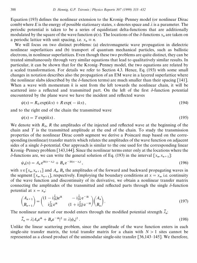
Equation (193) defines the nonlinear extension to the Kronig—Penney model (or nonlinear Diraccomb) where E is the energy of possible stationary states, x denotes space and j is a parameter. Theperiodic potential is taken to be a series of equidistant delta-functions that are additionallymodulated by the square of the wave function t(x). The locations of the d-functions x

nare taken on

a periodic lattice with unit spacing, i.e. xn,n.

We will focus on two distinct problems: (a) electromagnetic wave propagation in dielectricnonlinear superlattices and (b) transport of quantum mechanical particles, such as ballisticelectrons, in nonlinear superlattices. Even though these two problems are quite distinct, they can betreated simultaneously through very similar equations that lead to qualitatively similar results. Inparticular, it can be shown that for the Kronig—Penney model, the two equations are related bya scaled transformation. For details we refer to Section 4.3. Hence, Eq. (193) with some smallchanges in notation describes also the propagation of an EM wave in a layered superlattice wherethe nonlinear slabs (described by the d-function terms) are much smaller than their spacing [141].When a wave with momentum k is sent from the left towards the nonlinear chain, it will bescattered into a reflected and transmitted part. On the left of the first d-function potentialencountered by the plane wave we have the incident and reflected waves

t(x)"R0exp(ikx)#R exp(!ikx) , (194)

and to the right end of the chain the transmitted wave

t(x)"¹ exp(ikx) . (195)

We denote with R0, R the amplitudes of the injected and reflected wave at the beginning of the

chain and ¹ is the transmitted amplitude at the end of the chain. To study the transmissionproperties of the nonlinear Dirac comb segment we derive a Poincare map based on the corre-sponding (nonlinear) transfer matrix which relates the amplitudes of the wave function on adjacentsides of a single d-potential. Our approach is similar to the one used for the corresponding linearKronig—Penney problem [143,144]. Since the nonlinear terms enter only at the locations where thed-functions are, we can write the general solution of Eq. (193) in the interval [x

n, x

n`1]:

tn(x)"A

ne*k(x~xn)#B

ne~*k(x~xn) , (196)

with x3[xn,x

n`1] and A

n, B

nthe amplitudes of the forward and backward propagating waves in

the segment [xn, x

n`1], respectively. Employing the boundary conditions at x"x

n, i.e. continuity

of the wave function and discontinuity of its derivative, we obtain a nonlinear transfer matrixconnecting the amplitudes of the transmitted and reflected parts through the single d-functionpotential at x"x

n:

AA

n`1Bn`1B"A

(1!ijI n2k

)e*k !ijI n2k

e~*k

ijI n2k

e*k (1#ijI n2k

) e~*kBAA

nB

nB . (197)

The nonlinear nature of our model enters through the modified potential strength jIn:

jIn"jDA

ne*k#B

ne~*kD2,jD/

nD2 . (198)

Unlike the linear scattering problem, since the amplitude of the wave function enters in eachsingle-site transfer matrix, the total transfer matrix for a chain with N'1 sites cannot berepresented as a closed product of the unimodular single-site transfer [36,143—145]. We therefore,


need to iterate the Poincare map (An, B

n)P(A

n`1,B

n`1) of Eq. (197) repeatedly for n"1,2, N.

Computations are facilitated if we first transform the matrix relation of Eq. (197) to a differenceequation [143]. We use the transformation

A/n`1/

nB"A

e*k e~*k

1 1 BAA

nB

nB , (199)

to go from the “bond variables” (An, B

n) to the “node” variables (/

n, /

n`1). The combined use of

Eqs. (197)—(199) leads to a second order nonlinear difference equation for the node variables /n:

/n`1

#/n1"C2 cos(k)#j

sin(k)k

D/nD2D/n

. (200)

Eq. (200) is formally identical to the stationary discrete nonlinear Schrodinger equation (DNLS)with on-site energy E(k)"2 cos(k), unit transfer matrix element and nonlinearity parameterj(sin(k)/k) [1]. In fact there exist a connection between difference equations (tight-binding models)and differential Schrodinger equations [146,147]. For example Belissard et al. [143] showed thatthe Schrodinger equation for a periodic array of delta functions of potentials which can beincommensurate with the lattice of delta functions is equivalent to the Aubry model, that isa difference equation with a quasiperiodic potential [40].

We can utilize the equivalence of Eq. (200) with the DNLS equation of Section 2.1 to reduce thedynamics again to a two dimensional (real-valued) map going along the same lines as described inSection 2.4 to obtain a map (x

n, z

n)P(x

n~1, z

n~1) where we study from the beginning the inverse

map:

xn~1

"C2 cos(k)#jsin(k)2k

(¼n!z

n)D(¼n

!zn)!x

n, (201)

zn~1

"

12

x2n!x2

n~1¼

n!z

n

!zn, (202)

with ¼n"Jx2

n#z2

n#4J2.

In Fig. 9 we show a number of orbits of the map. The elliptic fixed points of the period-4 islandchain are surrounded by (regular) quasiperiodic orbits whereas in the vicinity of the separatrix ofthe hyperbolic fixed points a thin chaotic layer develops. The evolution of the wave amplituder2n

corresponding to a chaotic orbit in Fig. 9 is illustrated in Fig. 10.In Fig. 11 we illustrate the transmission behavior of a nonlinear chain with 500 d-potentials in

the k!D¹D2 plane. This representation is similar to that used by Delyon et al. and Wan andSoukoulis in the study of the corresponding “one-band” tight binding model [81,82]. For a givenoutput plane wave with intensity D¹D2 and momentum k the mapping of Eqs. (201) and (202) hasbeen iterated. For incoming wave intensities DR

0D2 that are of the same order of the transmitted

intensity the nonlinear chain is said to be transmitting (black area in Fig. 11). A divergent solution,on the other hand, results to absence of transmission (white area in Fig. 11). The curve separatingthe two different regimes in the k!D¹D2 plane exhibits a rich structure. For momenta k"np


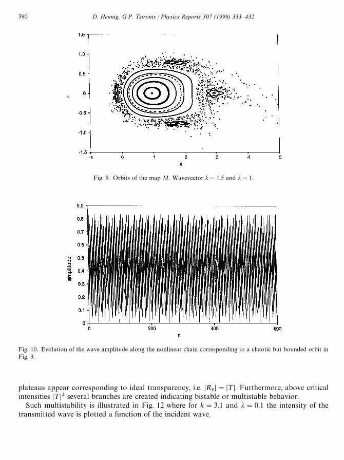
Fig. 9. Orbits of the map M. Wavevector k"1.5 and j"1.

Fig. 10. Evolution of the wave amplitude along the nonlinear chain corresponding to a chaotic but bounded orbit inFig. 9.

plateaus appear corresponding to ideal transparency, i.e. DR0D"D¹D. Furthermore, above critical

intensities D¹D2 several branches are created indicating bistable or multistable behavior.Such multistability is illustrated in Fig. 12 where for k"3.1 and j"0.1 the intensity of the

transmitted wave is plotted a function of the incident wave.


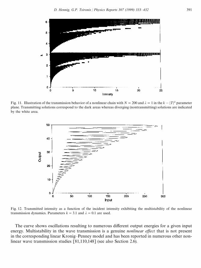
Fig. 11. Illustration of the transmission behavior of a nonlinear chain with N"200 and j"1 in the k!D¹D2 parameterplane. Transmitting solutions correspond to the dark areas whereas diverging (nontransmitting) solutions are indicatedby the white area.

Fig. 12. Transmitted intensity as a function of the incident intensity exhibiting the multistability of the nonlineartransmission dynamics. Parameters k"3.1 and j"0.1 are used.

The curve shows oscillations resulting to numerous different output energies for a given inputenergy. Multistability in the wave transmission is a genuine nonlinear effect that is not presentin the corresponding linear Kronig—Penney model and has been reported in numerous other non-linear wave transmission studies [81,110,148] (see also Section 2.6).


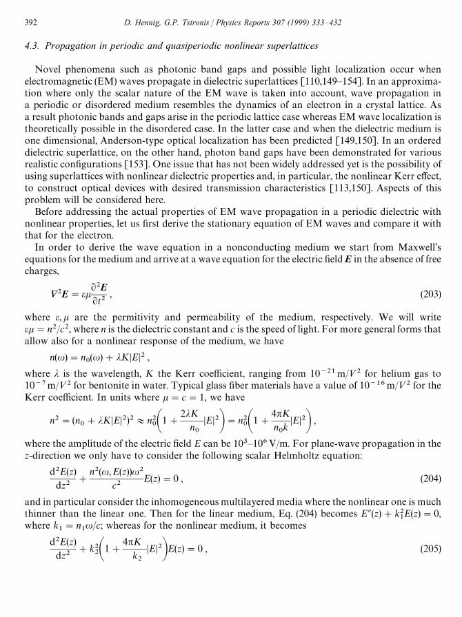
4.3. Propagation in periodic and quasiperiodic nonlinear superlattices

Novel phenomena such as photonic band gaps and possible light localization occur whenelectromagnetic (EM) waves propagate in dielectric superlattices [110,149—154]. In an approxima-tion where only the scalar nature of the EM wave is taken into account, wave propagation ina periodic or disordered medium resembles the dynamics of an electron in a crystal lattice. Asa result photonic bands and gaps arise in the periodic lattice case whereas EM wave localization istheoretically possible in the disordered case. In the latter case and when the dielectric medium isone dimensional, Anderson-type optical localization has been predicted [149,150]. In an ordereddielectric superlattice, on the other hand, photon band gaps have been demonstrated for variousrealistic configurations [153]. One issue that has not been widely addressed yet is the possibility ofusing superlattices with nonlinear dielectric properties and, in particular, the nonlinear Kerr effect,to construct optical devices with desired transmission characteristics [113,150]. Aspects of thisproblem will be considered here.

Before addressing the actual properties of EM wave propagation in a periodic dielectric withnonlinear properties, let us first derive the stationary equation of EM waves and compare it withthat for the electron.

In order to derive the wave equation in a nonconducting medium we start from Maxwell’sequations for the medium and arrive at a wave equation for the electric field E in the absence of freecharges,

+2E"ek2Et2

, (203)

where e,k are the permitivity and permeability of the medium, respectively. We will writeek"n2/c2, where n is the dielectric constant and c is the speed of light. For more general forms thatallow also for a nonlinear response of the medium, we have

n(u)"n0(u)#jKDED2 ,

where j is the wavelength, K the Kerr coefficient, ranging from 10~21m/»2 for helium gas to10~7m/»2 for bentonite in water. Typical glass fiber materials have a value of 10~16m/»2 for theKerr coefficient. In units where k"c"1, we have

n2"(n0#jKDED2)2+n2

0A1#2jK

n0

DED2B"n20A1#

4pKn0k

DED2B ,

where the amplitude of the electric field E can be 103—106V/m. For plane-wave propagation in thez-direction we only have to consider the following scalar Helmholtz equation:

d2E(z)dz2

#

n2(u,E(z))u2

c2E(z)"0 , (204)

and in particular consider the inhomogeneous multilayered media where the nonlinear one is muchthinner than the linear one. Then for the linear medium, Eq. (204) becomes EA(z)#k2

1E(z)"0,

where k1"n

1u/c; whereas for the nonlinear medium, it becomes

d2E(z)dz2

#k22A1#

4pKk2

DED2BE(z)"0 , (205)


where k2"n

2u/c. In the context of the Kronig—Penney model with wavenumber k"k

1, we get

k2E(z)"!

d2E(z)dz2

#

N+n/1

k2d(z!zn)g(E(z))E(z) , (206)

where

g(E(z))"1!a2!4paK

kDE(z)D2, and a"n

2/n

1. (207)

Upon comparison with Eq. (205) we note the following similarities and differences: The role of thestationary energy E of the nonlinear Schrodinger equation of Eq. (205) is played by the wavenum-ber k2 or frequency u2 in the problem of wave propagation. Furthermore, whereas in the wave casethis term k2 appears as a factor in the delta-function term, this is not true for the particle case. Infact, it can be shown that Eq. (205) can be transformed into the same form as Eq. (206). In thetime-independent case the Maxwell’s equations for EM waves is reduced to the following equation:

!

d2/(x)dx2

#k2+n

d(x!na)g(n)/(x)"k2/(x) , (208)

where /(x) is the complex electric field strength, k is the wavenumber of the wave andg(n),g(n, D/D2) is the term that modifies nonlinearly the d-function strengths. The motion ofparticles, on the other hand, is describable by the one-dimensional Schrodinger equation:

!

d2t(x)dx2

#+n

d(x!na)h(n)t(x)"Et(x) , (209)

where t(x) is the wave amplitude, E is the energy and h(n),h(n, DtD2) modifies the d-functionstrengths.

Let us define z"kx, and transform Eq. (208) into an equation with respect to the new variable z.Eq. (208) becomes

!

d2/(z)dz2

#k+n

d(z!nka)g(n)/(z)"/(z) . (210)

For particles with positive eigenenergy, E'0, if we define i"JE, and z"ix, Eq. (209) becomes

!

d2t(z)dz2

#

1i+n

d(z!nia)h(n)t(z)"t(z) . (211)

It is easy to see that Eqs. (210) and (211) will be in the same form, if we define the new d-functionstrengths g(n, k)"kg(n) and h(n,i)"h(n)/i, and substitute them into Eqs. (210) and (211), respec-tively. We note that the Schrodinger representation is more general since the classical wavepresentation corresponds only to the E'0 solutions of the former.

Due to this equivalence between the one-dimensional particle and classical wave problem, inwhat follows we will deal primarily with the Schrodinger representation of our problem. But firstwe will actually compare explicitly the two cases.


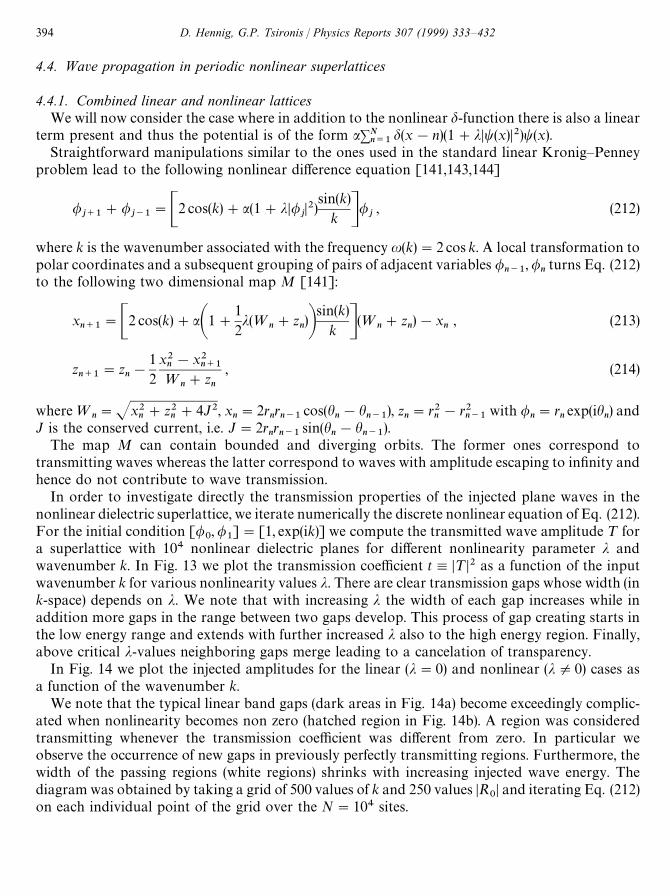
4.4. Wave propagation in periodic nonlinear superlattices

4.4.1. Combined linear and nonlinear latticesWe will now consider the case where in addition to the nonlinear d-function there is also a linear

term present and thus the potential is of the form a+Nn/1

d(x!n)(1#jDt(x)D2)t(x).Straightforward manipulations similar to the ones used in the standard linear Kronig—Penney

problem lead to the following nonlinear difference equation [141,143,144]

/j`1

#/j~1

"C2 cos(k)#a(1#jD/jD2)

sin(k)k D/j

, (212)

where k is the wavenumber associated with the frequency u(k)"2 cos k. A local transformation topolar coordinates and a subsequent grouping of pairs of adjacent variables /

n~1, /

nturns Eq. (212)

to the following two dimensional map M [141]:

xn`1

"C2 cos(k)#aA1#12j(¼

n#z

n)B

sin(k)k D(¼n

#zn)!x

n, (213)

zn`1

"zn!

12

x2n!x2

n`1¼

n#z

n

, (214)

where ¼n"Jx2

n#z2

n#4J2, x

n"2r

nrn~1

cos(hn!h

n~1), z

n"r2

n!r2

n~1with /

n"r

nexp(ih

n) and

J is the conserved current, i.e. J"2rnrn~1

sin(hn!h

n~1).

The map M can contain bounded and diverging orbits. The former ones correspond totransmitting waves whereas the latter correspond to waves with amplitude escaping to infinity andhence do not contribute to wave transmission.

In order to investigate directly the transmission properties of the injected plane waves in thenonlinear dielectric superlattice, we iterate numerically the discrete nonlinear equation of Eq. (212).For the initial condition [/

0, /

1]"[1, exp(ik)] we compute the transmitted wave amplitude ¹ for

a superlattice with 104 nonlinear dielectric planes for different nonlinearity parameter j andwavenumber k. In Fig. 13 we plot the transmission coefficient t,D¹D2 as a function of the inputwavenumber k for various nonlinearity values j. There are clear transmission gaps whose width (ink-space) depends on j. We note that with increasing j the width of each gap increases while inaddition more gaps in the range between two gaps develop. This process of gap creating starts inthe low energy range and extends with further increased j also to the high energy region. Finally,above critical j-values neighboring gaps merge leading to a cancelation of transparency.

In Fig. 14 we plot the injected amplitudes for the linear (j"0) and nonlinear (jO0) cases asa function of the wavenumber k.

We note that the typical linear band gaps (dark areas in Fig. 14a) become exceedingly complic-ated when nonlinearity becomes non zero (hatched region in Fig. 14b). A region was consideredtransmitting whenever the transmission coefficient was different from zero. In particular weobserve the occurrence of new gaps in previously perfectly transmitting regions. Furthermore, thewidth of the passing regions (white regions) shrinks with increasing injected wave energy. Thediagram was obtained by taking a grid of 500 values of k and 250 values DR

0D and iterating Eq. (212)

on each individual point of the grid over the N"104 sites.


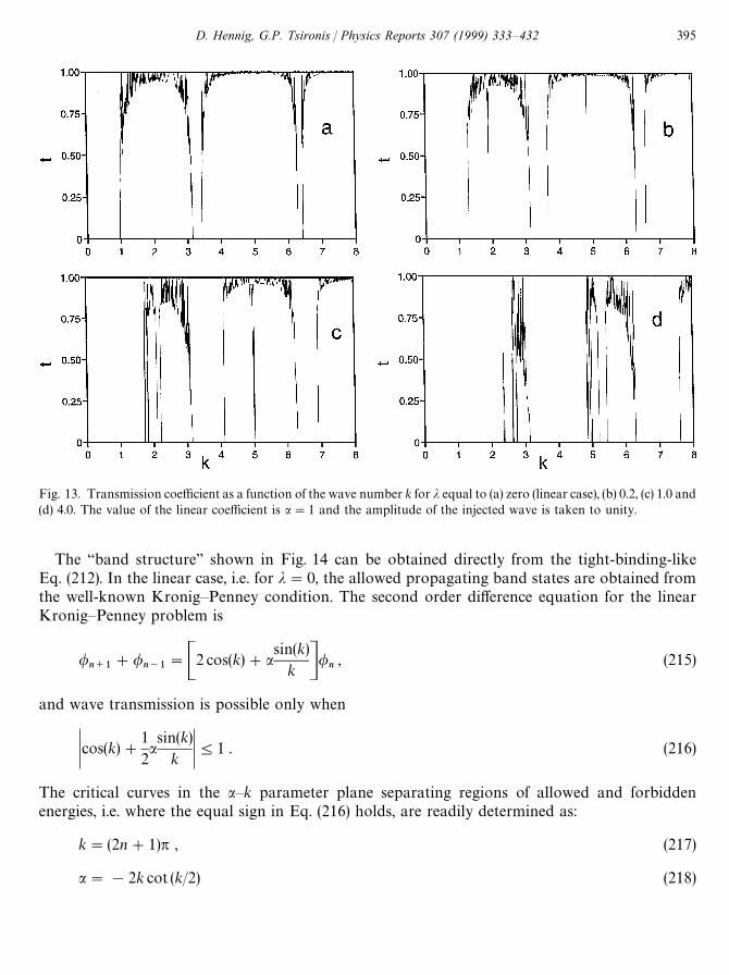
Fig. 13. Transmission coefficient as a function of the wave number k for j equal to (a) zero (linear case), (b) 0.2, (c) 1.0 and(d) 4.0. The value of the linear coefficient is a"1 and the amplitude of the injected wave is taken to unity.

The “band structure” shown in Fig. 14 can be obtained directly from the tight-binding-likeEq. (212). In the linear case, i.e. for j"0, the allowed propagating band states are obtained fromthe well-known Kronig—Penney condition. The second order difference equation for the linearKronig—Penney problem is

/n`1

#/n~1

"C2 cos(k)#asin(k)

k D/n, (215)

and wave transmission is possible only when

Kcos(k)#12asin(k)

k K41 . (216)

The critical curves in the a—k parameter plane separating regions of allowed and forbiddenenergies, i.e. where the equal sign in Eq. (216) holds, are readily determined as:

k"(2n#1)p , (217)

a"!2k cot (k/2) (218)


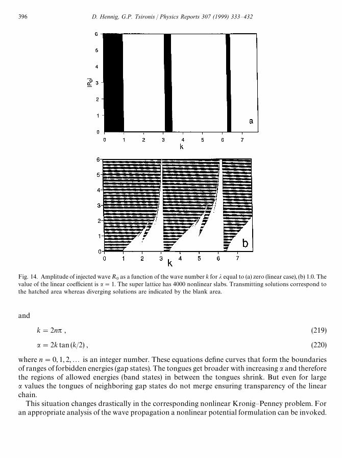
Fig. 14. Amplitude of injected wave R0as a function of the wave number k for j equal to (a) zero (linear case), (b) 1.0. The

value of the linear coefficient is a"1. The super lattice has 4000 nonlinear slabs. Transmitting solutions correspond tothe hatched area whereas diverging solutions are indicated by the blank area.

and

k"2np , (219)

a"2k tan (k/2) , (220)

where n"0, 1, 2,2 is an integer number. These equations define curves that form the boundariesof ranges of forbidden energies (gap states). The tongues get broader with increasing a and thereforethe regions of allowed energies (band states) in between the tongues shrink. But even for largea values the tongues of neighboring gap states do not merge ensuring transparency of the linearchain.

This situation changes drastically in the corresponding nonlinear Kronig—Penney problem. Foran appropriate analysis of the wave propagation a nonlinear potential formulation can be invoked.


To this end we exploit the fact that Eq. (212) can be derived by a variational approach ¸//*n"0,

where the Lagrangian is given by

¸"+n

(/*n(/

n`1#/*

n`1/n)!+

nC2 cos(k)#aA1#j

sin(k)2k

D/nD2BDD/n

D2 . (221)

The first kinetic term on the r.h.s. of Eq. (221) is responsible for the transfer along the chain whereasthe second term represents the local on-site potentials º(D/

nD) which are of Landau—Ginsburg type.

These quartic on-site potentials obey radial symmetry and are either convex (for E"2 cos(k)'0)or concave (for E"2 cos(k)(0). For a discussion of the stability of the wave dynamics evolving insuch a potential we first locate the extrema of the potential which follow from º/D/

nD"0. In the

linear Kronig problem the quadratic potential is

º-*/

(D/nD)"C2 cos(k)#a

sin(k)k DD/n

D2 . (222)

There is always a global minimum at

D/I D"0 . (223)

In the nonlinear case, the quartic potential reads as

º/0/-*/

(D/nD)"C2 cos(k)#aA1#j

sin(k)2k

D/nD2BDD/n

D2 , (224)

and the minimum remains at D/I D"0. For k3[np,(2n#1)p/2) the minimum is the global extremumof the potential so that the potential exhibits the same features as in the linear case. In accordancewith the condition for linear stability we require analogous to the treatment in Section 2.3 for wavepropagation the constraint

Kcos(k)#12aA1#j

sin(k)2k

D/D2BK41 . (225)

The instability tongues in the present nonlinear case are broadened indicating stronger parameterinstability. This is due to the explicit occurrence of the nonlinearity term on the l.h.s. in Eq. (225) sothat the boundaries of the instability tongues in the k—a parameter plane become also waveamplitude dependent:

k"(2n#1)p, (226)

a"!2 cotAk2B(1#jD/D2) , (227)

and

k"2np , (228)

a"2k tanAk2B(1#jD/D2) . (229)


Due to the fact that in these k-intervals wave instability is caused by exceeding an energetic stabilityborder like in the linear case we refer to the corresponding tongues as linear instability tongues.

For k3[(2n!1)p/2, np) and cos(k)(!a/2 a bifurcation appears and the potential has globalmaxima at

D/InD"S!A

2 cos(k)a

#1Bk

j sin(k), (230)

yielding a set of unstable equilibria. Therefore we have a ring of homoclinic fixed points/I "RI exp(iH) characterized by the radii D/I D and different values of the phase H3[0, 2p). Thedynamics of the wave amplitude in the proximity of the homoclinic structure exhibits extremesensitivity in the choice of the initial momenta k inducing thus “spatial” chaos in the wavetransmission. The instability in the proximity separatrix motion manifests itself in a “transient”phase of irregular homoclinic oscillations in the amplitude dynamics. Once the amplitude exceedsthe separatrix threshold it blows up to infinity giving rise to a gap state. Due to the nature of theescape process we call the corresponding instability tongues homoclinic instability tongues.

Above critical D/D-values the linear instability tongues and the corresponding neighboringhomoclinic instability tongues merge at k"(2n#1)p/2 creating broad forbidden gaps thusleading to impenetrability of the nonlinear chain. This is a purely nonlinear effect that is not presentin the linear Kronig—Penney model. In the latter there are always allowed bands however smallthey might be.

In conclusion one sees that nonlinearity in Kronig—Penney models, arising from strong many-body effects in the electron propagation [155] leads not only to multistability in the transmission ofplane waves but also has profound effects on the overall transparency of the chain. While thenonlinear model is not very different from the corresponding linear one in the very small D/D regime(respectively j regime), the former exhibits non-transparency for larger D/D-values: A criticalthreshold in the values of D/D exists above which the lattice becomes opaque to all wave transmis-sion. If we compare the “band structures” of the linear and nonlinear Kronig—Penney models foreach wavenumber k and corresponding parameter j-values we observe an overall reduction intransmittance in the nonlinear case. Furthermore, we note the appearance of new propagation gapsin the nonlinear case in wavevector regions where there was previously (in the linear case),a transmitting band. This behavior is markedly different from the one reported by Chen and Mills[111] and Kahn et al. [96] in a similar system. The difference, however, lies in the fact that while inthe present case we are investigating plane wave propagation, in reference [111] soliton-likemotion is studied. The presence of nonlinearity in the latter case assists the solitary wavepropagation even at locations inside the gap of the corresponding linear problem. The conclusionreached by comparing these two problems is similar to that obtained in other cases, viz. that ina discrete nonlinear medium wavepackets and modes with bounded support travel more efficientlythan plane waves [156].

The presence of nonlinearity in the dielectric superlattice planes alters substantially the transmis-sion properties of the waves. In particular, when the input power D/

0D (nonlinear coefficient j) is

increased new nontransmitting regions appear adjacent to the regular instability regions. Conse-quently, for a given wavenumber k, an appropriate change of the input power of the wave(corresponding to a change in j) can switch the wave from a transmitting to a nontransmitting


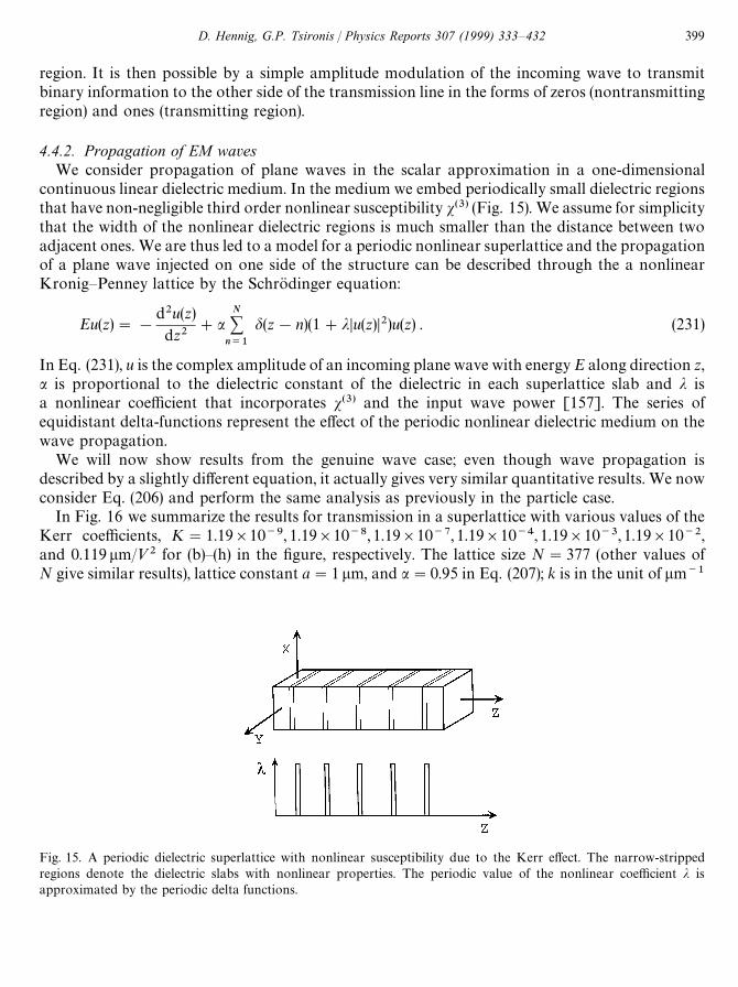
Fig. 15. A periodic dielectric superlattice with nonlinear susceptibility due to the Kerr effect. The narrow-strippedregions denote the dielectric slabs with nonlinear properties. The periodic value of the nonlinear coefficient j isapproximated by the periodic delta functions.

region. It is then possible by a simple amplitude modulation of the incoming wave to transmitbinary information to the other side of the transmission line in the forms of zeros (nontransmittingregion) and ones (transmitting region).

4.4.2. Propagation of EM wavesWe consider propagation of plane waves in the scalar approximation in a one-dimensional

continuous linear dielectric medium. In the medium we embed periodically small dielectric regionsthat have non-negligible third order nonlinear susceptibility s(3) (Fig. 15). We assume for simplicitythat the width of the nonlinear dielectric regions is much smaller than the distance between twoadjacent ones. We are thus led to a model for a periodic nonlinear superlattice and the propagationof a plane wave injected on one side of the structure can be described through the a nonlinearKronig—Penney lattice by the Schrodinger equation:

Eu(z)"!

d2u(z)dz2

#aN+n/1

d(z!n)(1#jDu(z)D2)u(z) . (231)

In Eq. (231), u is the complex amplitude of an incoming plane wave with energy E along direction z,a is proportional to the dielectric constant of the dielectric in each superlattice slab and j isa nonlinear coefficient that incorporates s(3) and the input wave power [157]. The series ofequidistant delta-functions represent the effect of the periodic nonlinear dielectric medium on thewave propagation.

We will now show results from the genuine wave case; even though wave propagation isdescribed by a slightly different equation, it actually gives very similar quantitative results. We nowconsider Eq. (206) and perform the same analysis as previously in the particle case.

In Fig. 16 we summarize the results for transmission in a superlattice with various values of theKerr coefficients, K"1.19]10~9, 1.19]10~8, 1.19]10~7, 1.19]10~4, 1.19]10~3, 1.19]10~2,and 0.119lm/»2 for (b)—(h) in the figure, respectively. The lattice size N"377 (other values ofN give similar results), lattice constant a"1lm, and a"0.95 in Eq. (207); k is in the unit of lm~1


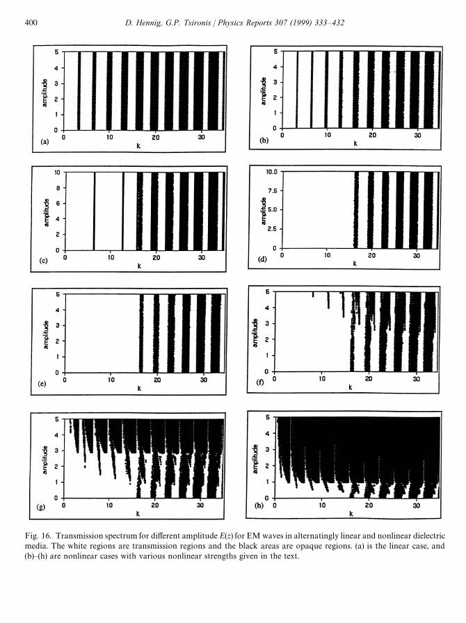
Fig. 16. Transmission spectrum for different amplitude E(z) for EM waves in alternatingly linear and nonlinear dielectricmedia. The white regions are transmission regions and the black areas are opaque regions. (a) is the linear case, and(b)—(h) are nonlinear cases with various nonlinear strengths given in the text.


and the field amplitude E(z) is in the unit of V/lm. We note the qualitative similarity in thetransmission properties with the particle case. In addition, we see also a new feature in the “weak”nonlinearity cases. There is a region where nonlinearity reduces the widths of the gaps and in somecases it effectively eliminates them for small k’s. This means that the transparency of the medium isenhanced in this particular region. We note that for large nonlinearity values the medium becomesopaque for large values of k.

4.5. Transmission in a quasiperiodic lattice-I

We review the work on quasiperiodic nonlinear Kronig—Penney models with a sequence ofbarrier heights as well as sequential intersite distances constructed according to the Fibonacciinflation rule. We find that nonlinearity enhances transparency and reduces the localizationproperties of the corresponding linear quasiperiodic Kronig—Penney model.

Since the discovery of the quasi-crystalline phase in AlMn exhibiting quasiperiodic propertiesthere has been growing interest in models describing the electron and phonon spectrum of suchquasicrystals [158]. Recent advances in nanodevice manufacturing has increased the interest inquasiperiodic one dimensional models [159]. Merlin et al. synthesized the first one dimensionalsemiconductor superlattice [160]. Quasiperiodic models provide a bridge between the regularordered lattices of perfect materials and random lattices of amorphous systems. Interest inelectronic propagation in quasicrystals has led to a thorough investigation of the band structure ofsome quasiperiodic systems, such as Penrose tiling and Fibonacci lattices [161—163]. Concerningthe localization problem for wave propagation within a linear theory there exist three types of wavefunctions: localized (normalizable), extended (unnormalizable) and critical. For (electronic) tight-binding models possessing either two types of hopping matrix elements or on-site energy arrangedin a Fibonacci sequence one obtains a Cantor-set of allowed energies and the wave function isself-similar and therefore intermediate between a localized and extended state [36,164]. Forelectron transmission in a one dimensional quasicrystal described by a (linear) Kronig—Penneymodel with d-potentials heights arranged due to the Fibonacci sequence two kinds of electronenergies exist. One correspond to localized states and the other two extended states [165].

Studies on combined effects of nonlinearity and quasiperiodicity on the optical transmissionproperties of superlattices consisting of nonlinear materials arranged in a Fibonacci sequence wereperformed in references by Kahn et al. in [166] and Gupta and Ray [167]. Special attention waspaid whether the gap solitons which had been found in the corresponding periodic nonlinear latticeexist in the aperiodic case as well. Kahn et al. [166] using a tight-binding like model found noevidence for gap solitons the field envelops turn out to be rather irregular and fast oscillating.Gupta and Ray utilized a nonlinear transfer matrix technique under the assumption of slowlyvarying envelope functions and established the existence of gap solitons for a choice of the linearoptical path in each slab as np with integer n. But in these parameter ranges the linear transmissionis also perfect since it remains unaffected by the quasiperiodicity. Later Johannsson and Riklundstudied the electronic transmission properties of a one dimensional deterministic aperiodic nonlin-ear tight-binding lattice based on the DNLS. Quasiperiodicity in their model enters througharrangements of the on-site energy according to the Thue—Morse sequence [168]. For smallnonlinearity the authors found soliton-like solutions in a similar way as in the correspondingperiodic model. Contrary to the Fibonacci type aperiodicity the Thue—Morse type aperiodicity


supports transmission in the gaps of the linear regime in the form of gap solitons. With respect tothe existence of single-site self-trapped states in aperiodic nonlinear discrete systems Johansson andRiklund concluded from their numerical analysis that there seems to be always self-trappingwhenever in the corresponding linear lattice the spectrum is a point spectrum or a singularcontinuous spectrum. Finally, Hiramoto and Kohmoto extended a linear quasiperiodic tightbinding model by adding a Hubbard-type interaction term giving so rise to nonlinearity in themodel. They showed that such a term does not affect the Cantor-set character of the spectrum fora Fibonacci model and hence the wave functions stay critical. However for the incommensurateAubry model the singular continuous character of the spectrum becomes destroyed [163,169].

In the present section we will be addressing the issue of wave propagation in a quasiperiodicsuperlattice model where the medium has in addition nonlinear properties arising from the opticalKerr effect [113,141,150]. We will study the interplay between nonlinearity and quasiperiodicityand demonstrate that it can be used advantageously in wave propagation in nanodevices. Theresults obtained are also applicable to problems of electronic propagation in superlattices wherethe effective nonlinearity stems from many-body interactions [155].

We consider the following general Kronig—Penney equation:

!

d2t(z)dz2

#

N+n/1

jnd(z!z

n)g(z)t(z)"Et(z) , (232)

where for the linear (L), nonlinear (NL) and the general nonlinear (GNL) models, we define asfollows:

g(z)"G1, L

Dt(z)D2, NL

a0#a

1Dt(z)D2, GNL ,

where (a0, a

1) are real numbers.

In Eq. (232), t(z) represents an electronic wavefunction or is the complex amplitude of anincoming plane wave with energy (or frequency) E along direction z, and j

nis a coefficient that, in

the case of the nonlinear optical medium, incorporates the nonlinear susceptibility s(3) and theinput wave power [141,157]. The space-periodic d-functions represent small nonlinear dielectricregions that are periodically embedded in a linear dielectric medium. These nonlinear regions areassumed to be much smaller than the distance between adjacent ones. Quasiperiodicity in thismodel enters in a twofold way. Firstly, the coefficients j

nthat are assumed to follow the Fibonacci

sequence. This sequence follows from the inflation rule: Sl`1

"SlSl~1

, where S0"A and S

1"AB.

There are only two values of jn, j

Aand j

Band the actual value of j

nat location n is determined from

the Fibonacci rule. We use the following procedure to obtain the sequence [144]:

kn`1

"[/n#1/c], /

n`1"(/

n#1/c) : mod(1) , (233)

where the rectangular brackets denote the integer part , c"(J5#1)/2 is the golden mean and westart with /

0"0 at n"1. The value of j

nis j

Aof j

Bwhen k

nis 1 or 0, respectively.

Secondly, the intersite distances dn"z

n!z

n~1are assumed to be quasiperiodic and follow the

Fibonacci sequence. There are two values of dn, d

n"1 or d

n"a'1 resulting from the actual


location of zn

which is determined by the rule

zn"n#(a!1)C

n#1u D

with u"(1#J5)/2 being the golden mean and the bracket [ ] denoting the integer part. Whenthe intersite distance d

nis a constant, it can be shown that finding the solution of Eq. (232) is

equivalent to solving the problem of a nonlinear tight-binding model [143,144]; but this is nolonger true for the quasiperiodic nonlinear lattices which are being studied here.

We investigate the scattering problem of a quasiparticle with momentum k. The first study dealswith the NL-case when quasiperiodicity enters through an arrangement of the heights of thedelta-barriers due to the Fibonacci sequence while the distances between them is kept constant.Plane waves are sent from the left towards the nonlinear chain and will be scattered into a reflectedand transmitted part.

Straightforward manipulations similar to the ones used in the standard linear Kronig—Penneyproblem lead to the following nonlinear difference equation for t

n,t(n) [141,143,144]

tn`1

#tn~1

"C2 cos(k)#jnDt

nD2sin(k)

k Dtn, (234)

where k is the wavenumber associated with the energy (or frequency) E(k)"2 cos(k). Eq. (234) canbe treated as a nonlinear map for various initial conditions corresponding to waves injectedinitially from the left and propagating towards the right side of the chain.

In Fig. 17 we illustrate the transmission behavior in the DR0D!k parameter plane for the linear

Fibonacci Kronig—Penney model (Fig. 17a) and the nonlinear one (Fig. 17b).Dark regions represent gaps in the wave propagation whereas the passing regions are white. In

the linear case, i.e. when the term DtnD2 is absent from Eq. (234), we have the typical band structure

resulting from quasiperiodicity [36]. We note that the effect of nonlinearity alters substantially thisstructure resulting in enhanced propagation for small initial intensities. The lattice is transparentfor essentially all wavenumbers k at low intensities. In particular, the dominant linear gap fork-values approximately less than k&2 is reduced drastically. In the higher intensity region, on theother hand, the forbidden lines seem to coalesce together to form well defined nonlinear gaps thatare interrupted periodically from propagating resonance-like zones. The latter occur for k-valuesthat are multiples of p; for these wavenumbers the nonlinear term is effectively canceled leading toperfect propagation.

The nonlinear lattice model we presented here has applications in the propagation of electrons insuperlattices and electromagnetic waves in the dielectric materials. In the latter case a quasiperiodiclinear term should also be included in Eq. (232) representing the linear dielectric constant of thematerial. The modification in the results due to this term will be studied below in the context of theGNL model.

4.6. Transmission in a quasiperiodic lattice-II

In the previous section, we have studied a lattice with spatially periodic potentials whosebivalued strengths are arranged in a quasiperiodic sequence [141]. It turned out that while


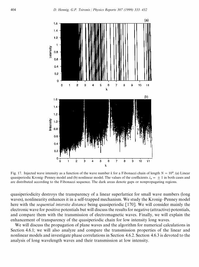
Fig. 17. Injected wave intensity as a function of the wave number k for a Fibonacci chain of length N"104. (a) Linearquasiperiodic Kronig—Penney model and (b) nonlinear model. The values of the coefficients j

n"$1 in both cases and

are distributed according to the Fibonacci sequence. The dark areas denote gaps or nonpropagating regions.

quasiperiodicity destroys the transparency of a linear superlattice for small wave numbers (longwaves), nonlinearity enhances it in a self-trapped mechanism. We study the Kronig—Penney modelhere with the sequential intersite distance being quasiperiodic [170]. We will consider mainly theelectronic wave for positive potentials but will discuss the results for negative (attractive) potentials,and compare them with the transmission of electromagnetic waves. Finally, we will explain theenhancement of transparency of the quasiperiodic chain for low intensity long waves.

We will discuss the propagation of plane waves and the algorithm for numerical calculations inSection 4.6.1; we will also analyze and compare the transmission properties of the linear andnonlinear models and investigate phase correlations in Section 4.6.2. Section 4.6.3 is devoted to theanalysis of long wavelength waves and their transmission at low intensity.


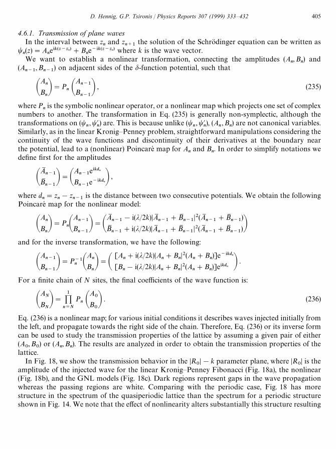
4.6.1. Transmission of plane wavesIn the interval between z

nand z

n`1the solution of the Schrodinger equation can be written as

tn(z)"A

ne*k(z~zn)#B

ne~*k(z~zn) where k is the wave vector.

We want to establish a nonlinear transformation, connecting the amplitudes (An, B

n) and

(An~1

, Bn~1

) on adjacent sides of the d-function potential, such that

AA

nBnB"P

n AA

n~1B

n~1B , (235)

where Pnis the symbolic nonlinear operator, or a nonlinear map which projects one set of complex

numbers to another. The transformation in Eq. (235) is generally non-symplectic, although thetransformations on (t

n, t@

n) are. This is because unlike (t

n,t@

n), (A

n,B

n) are not canonical variables.

Similarly, as in the linear Kronig—Penney problem, straightforward manipulations considering thecontinuity of the wave functions and discontinuity of their derivatives at the boundary nearthe potential, lead to a (nonlinear) Poincare map for A

nand B

n. In order to simplify notations we

define first for the amplitudes

AAM

n~1BMn~1B"A

An~1

e*kdn

Bn~1

e~*kdnB ,

where dn"z

n!z

n~1is the distance between two consecutive potentials. We obtain the following

Poincare map for the nonlinear model:

AA

nBnB"P

nAA

n~1Bn~1B"A

AMn~1

!i(j/2k)DAMn~1

#BMn~1

D2(AMn~1

#BMn~1

)

BMn~1

#i(j/2k)DAMn~1

#BMn~1

D2(AMn~1

#BMn~1

)Band for the inverse transformation, we have the following:

AA

n~1Bn~1B"P~1

n AA

nBnB"A

[An#i(j/2k)DA

n#B

nD2(A

n#B

n)]e~*kdn

[Bn!i(j/2k)DA

n#B

nD2(A

n#B

n)]e*kdn B .

For a finite chain of N sites, the final coefficients of the wave function is:

AA

NBNB"

1<n/N

Pn A

A0

B0B . (236)

Eq. (236) is a nonlinear map; for various initial conditions it describes waves injected initially fromthe left, and propagate towards the right side of the chain. Therefore, Eq. (236) or its inverse formcan be used to study the transmission properties of the lattice by assuming a given pair of either(A

0, B

0) or (A

n, B

n). The results are analyzed in order to obtain the transmission properties of the

lattice.In Fig. 18, we show the transmission behavior in the DR

0D!k parameter plane, where DR

0D is the

amplitude of the injected wave for the linear Kronig—Penney Fibonacci (Fig. 18a), the nonlinear(Fig. 18b), and the GNL models (Fig. 18c). Dark regions represent gaps in the wave propagationwhereas the passing regions are white. Comparing with the periodic case, Fig. 18 has morestructure in the spectrum of the quasiperiodic lattice than the spectrum for a periodic structureshown in Fig. 14. We note that the effect of nonlinearity alters substantially this structure resulting


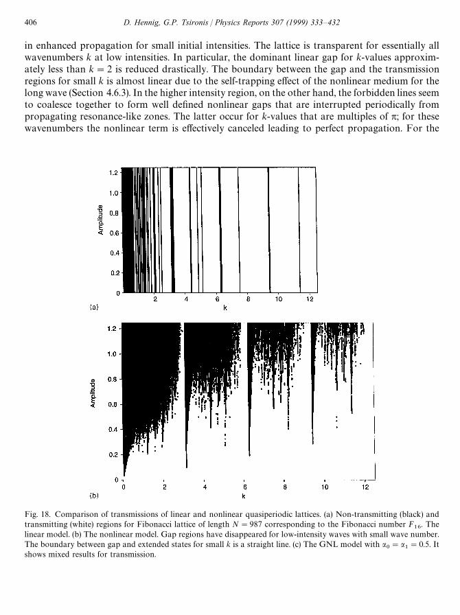
Fig. 18. Comparison of transmissions of linear and nonlinear quasiperiodic lattices. (a) Non-transmitting (black) andtransmitting (white) regions for Fibonacci lattice of length N"987 corresponding to the Fibonacci number F

16. The

linear model. (b) The nonlinear model. Gap regions have disappeared for low-intensity waves with small wave number.The boundary between gap and extended states for small k is a straight line. (c) The GNL model with a

0"a

1"0.5. It

shows mixed results for transmission.

in enhanced propagation for small initial intensities. The lattice is transparent for essentially allwavenumbers k at low intensities. In particular, the dominant linear gap for k-values approxim-ately less than k"2 is reduced drastically. The boundary between the gap and the transmissionregions for small k is almost linear due to the self-trapping effect of the nonlinear medium for thelong wave (Section 4.6.3). In the higher intensity region, on the other hand, the forbidden lines seemto coalesce together to form well defined nonlinear gaps that are interrupted periodically frompropagating resonance-like zones. The latter occur for k-values that are multiples of p; for thesewavenumbers the nonlinear term is effectively canceled leading to perfect propagation. For the


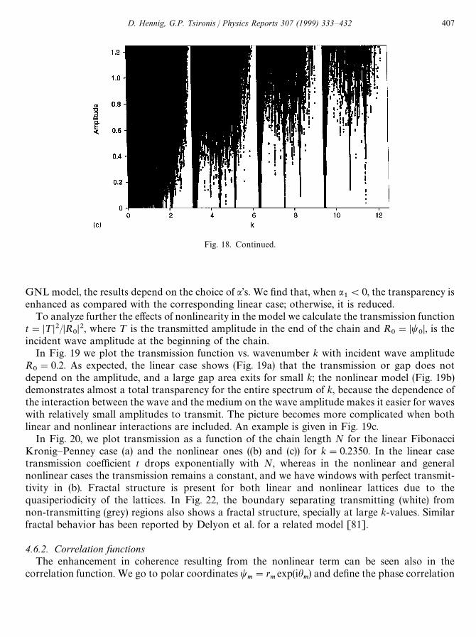
Fig. 18. Continued.

GNL model, the results depend on the choice of a’s. We find that, when a1(0, the transparency is

enhanced as compared with the corresponding linear case; otherwise, it is reduced.To analyze further the effects of nonlinearity in the model we calculate the transmission function

t"D¹D2/DR0D2, where ¹ is the transmitted amplitude in the end of the chain and R

0"Dt

0D, is the

incident wave amplitude at the beginning of the chain.In Fig. 19 we plot the transmission function vs. wavenumber k with incident wave amplitude

R0"0.2. As expected, the linear case shows (Fig. 19a) that the transmission or gap does not

depend on the amplitude, and a large gap area exits for small k; the nonlinear model (Fig. 19b)demonstrates almost a total transparency for the entire spectrum of k, because the dependence ofthe interaction between the wave and the medium on the wave amplitude makes it easier for waveswith relatively small amplitudes to transmit. The picture becomes more complicated when bothlinear and nonlinear interactions are included. An example is given in Fig. 19c.

In Fig. 20, we plot transmission as a function of the chain length N for the linear FibonacciKronig—Penney case (a) and the nonlinear ones ((b) and (c)) for k"0.2350. In the linear casetransmission coefficient t drops exponentially with N, whereas in the nonlinear and generalnonlinear cases the transmission remains a constant, and we have windows with perfect transmit-tivity in (b). Fractal structure is present for both linear and nonlinear lattices due to thequasiperiodicity of the lattices. In Fig. 22, the boundary separating transmitting (white) fromnon-transmitting (grey) regions also shows a fractal structure, specially at large k-values. Similarfractal behavior has been reported by Delyon et al. for a related model [81].

4.6.2. Correlation functionsThe enhancement in coherence resulting from the nonlinear term can be seen also in the

correlation function. We go to polar coordinates tm"r

mexp(ih

m) and define the phase correlation


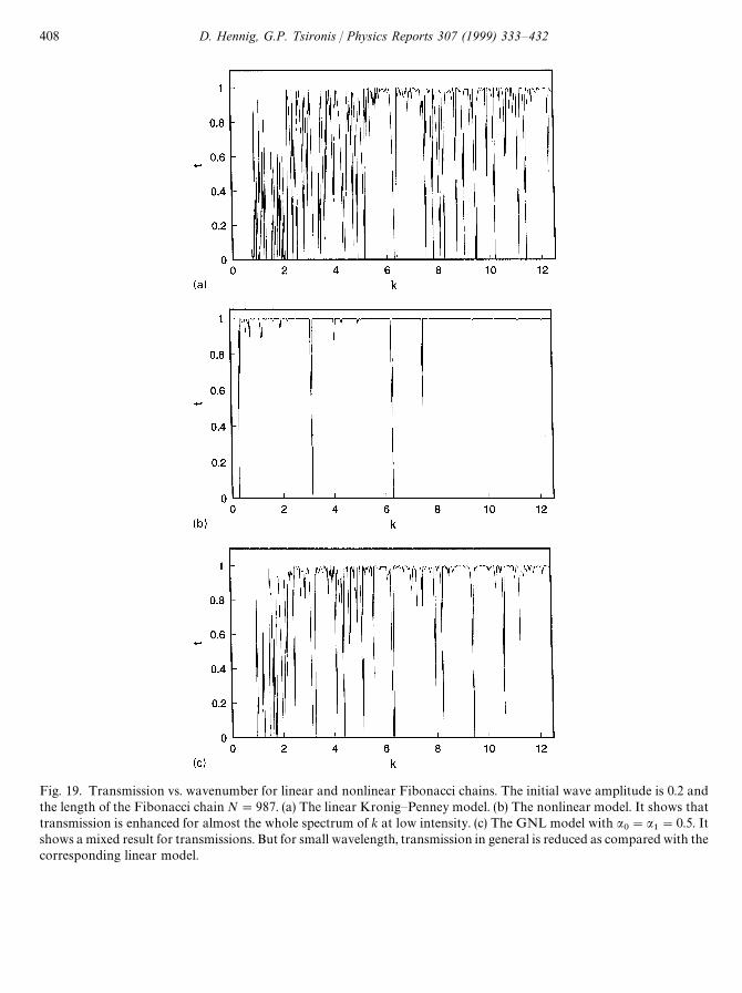
Fig. 19. Transmission vs. wavenumber for linear and nonlinear Fibonacci chains. The initial wave amplitude is 0.2 andthe length of the Fibonacci chain N"987. (a) The linear Kronig—Penney model. (b) The nonlinear model. It shows thattransmission is enhanced for almost the whole spectrum of k at low intensity. (c) The GNL model with a

0"a

1"0.5. It

shows a mixed result for transmissions. But for small wavelength, transmission in general is reduced as compared with thecorresponding linear model.


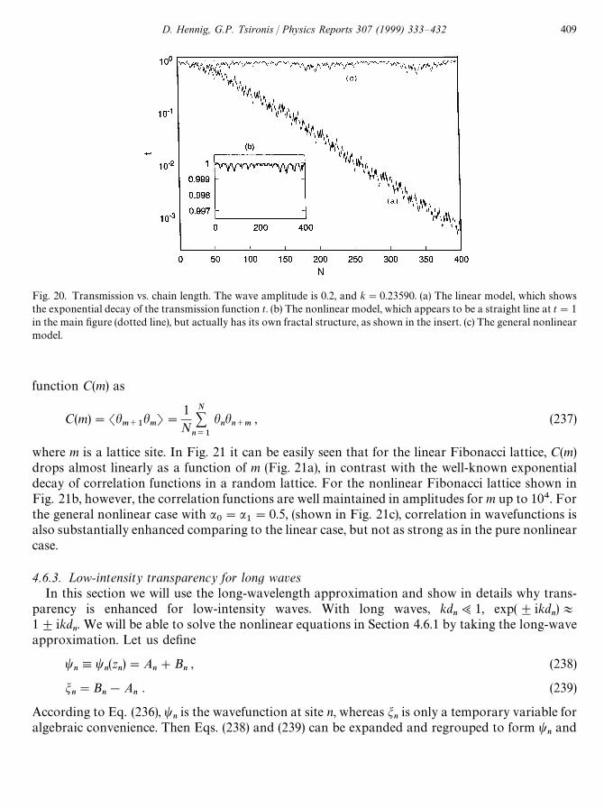
Fig. 20. Transmission vs. chain length. The wave amplitude is 0.2, and k"0.23590. (a) The linear model, which showsthe exponential decay of the transmission function t. (b) The nonlinear model, which appears to be a straight line at t"1in the main figure (dotted line), but actually has its own fractal structure, as shown in the insert. (c) The general nonlinearmodel.

function C(m) as

C(m)"Shm`1

hmT"

1N

N+n/1

hnhn`m

, (237)

where m is a lattice site. In Fig. 21 it can be easily seen that for the linear Fibonacci lattice, C(m)drops almost linearly as a function of m (Fig. 21a), in contrast with the well-known exponentialdecay of correlation functions in a random lattice. For the nonlinear Fibonacci lattice shown inFig. 21b, however, the correlation functions are well maintained in amplitudes for m up to 104. Forthe general nonlinear case with a

0"a

1"0.5, (shown in Fig. 21c), correlation in wavefunctions is

also substantially enhanced comparing to the linear case, but not as strong as in the pure nonlinearcase.

4.6.3. Low-intensity transparency for long wavesIn this section we will use the long-wavelength approximation and show in details why trans-

parency is enhanced for low-intensity waves. With long waves, kdn;1, exp($ikd

n)+

1$ikdn. We will be able to solve the nonlinear equations in Section 4.6.1 by taking the long-wave

approximation. Let us define

tn,t

n(z

n)"A

n#B

n, (238)

mn"B

n!A

n. (239)

According to Eq. (236), tnis the wavefunction at site n, whereas m

nis only a temporary variable for

algebraic convenience. Then Eqs. (238) and (239) can be expanded and regrouped to form tnand


Fig. 21. Phase correlation functions C(m) of propagating waves for three different quasiperiodic K—P models; (a) thelinear lattice, (b) nonlinear lattice, and (c) the GNL lattice. In the linear case, the amplitude of C(m) decays almost linearlywith m; in the nonlinear case, C(m) does not decay up to m"10 000; in the GNL case, C(m) drops more slowly than thelinear case. Notice different scales are used for (a)—(c).

mn, and by keeping only the first order terms, it is easy to see that

Gt

n"t

n~1!ikd

nmn~1

,

mn"m

n~1!ikd

nt

n#i

jkDt

nD2t

n.

(240)

Taking the continuum limit as kP0, or more appropriately, k~1<dn, Eq. (240) becomes a pair of

coupled differential equations:

dt(n)dn

"!ikm(n),dm(n)dn

"!ikt(n)#ijkd

Dt(n)D2t(n) , (241)


where we have replaced dnwith its average d. Substituting the second equation into the first one in

Eq. (241) after differentiation, we obtain the following second order differential wave equation:

t® (n)"!k2t(n)#jdDt(n)D2t(n) . (242)

We can distinguish three cases.¹he linear case. Replacing DtD2 with 1 in Eq. (242) yields the linear equation:

t® "!Ak2!jdBt,!p2t .

When p2(0, wavenumber k is small, there are only exponential solutions, which results inlocalized state. Roughly speaking, extended states will happen when k is in the order of k

%,Jj/d.

For example, in the previous section, we used j"1, d"1.618, so that k%"0.786, and this result is

consistent with Fig. 19a.¹he nonlinear case. Let t(n)"t

0exp[ipn] be a solution of Eq. (242), then we find

p2"k2!jdDt

0D2 . (243)

Unlike the linear case, whether p is real or imaginary now depends on the intensity of the waveDt

0D. As long as Dt

0D(Jj/d k, there will be propagating waves and hence extended states. Let

p"0, we have

Dt0D"Jj/d k . (244)

Eq. (244) represents the boundary that separates the gap state from the propagating state for verysmall k. Fig. 22 shows the result from numerical calculation which agrees with Eq. (244) for small k.We used j"1, and the average intersite distance d"1.618.

¹he general nonlinear case. Similarly, for the GNL model, the low-intensity wave equationbecomes:

t® "!Ak2!jd(a

0#a

1DtD2)Bt .

For solution of the type of t(n)"t0exp[ipn], we find

p2"k2!a0

jd!a

1

jdDt

0D2 .

Generally, transmission would be more difficult for small k because of the presence of the linearterm, and it will get worse if a

1'0. Compared with the corresponding linear model, better

transmission would be achieved for small wavenumber k, if the nonlinear term dominates over thelinear term, a

1<a

0.

The main result that we have shown in the last two sections is the enhancement of transmissionsat low wave intensities from a spatially quasiperiodic Kronig—Penney model, in which nonlinearityis added through doped layers in the case of electronic transport in a semiconductor superlattice, orKerr-type nonlinear media in the case of light transmission. Nonlinearity in the form contained in


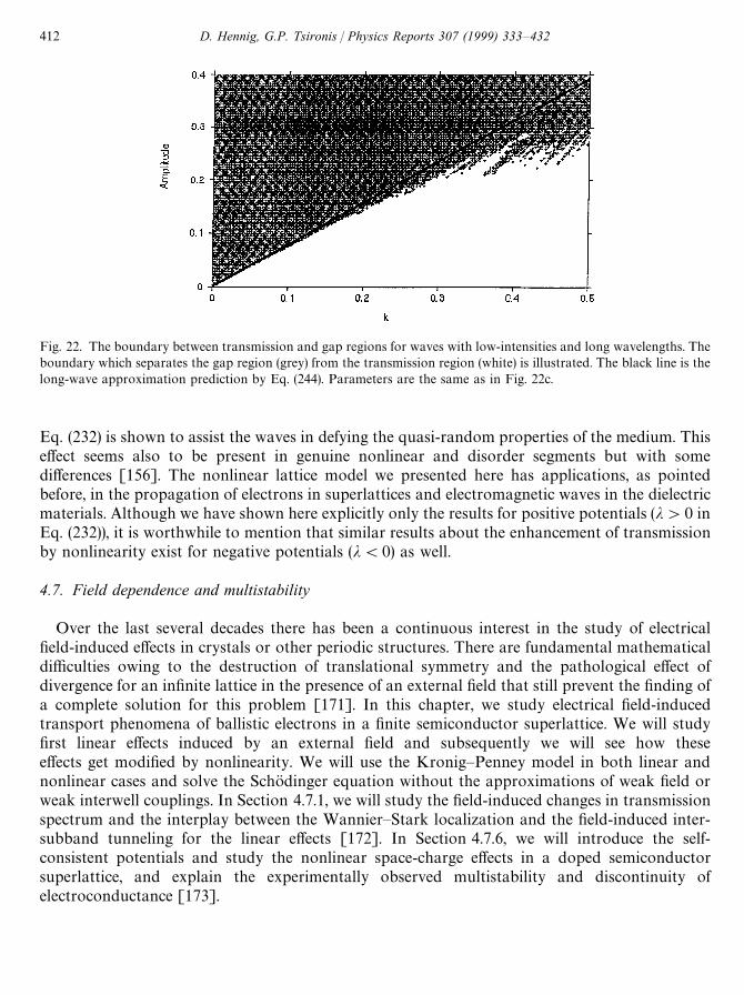
Fig. 22. The boundary between transmission and gap regions for waves with low-intensities and long wavelengths. Theboundary which separates the gap region (grey) from the transmission region (white) is illustrated. The black line is thelong-wave approximation prediction by Eq. (244). Parameters are the same as in Fig. 22c.

Eq. (232) is shown to assist the waves in defying the quasi-random properties of the medium. Thiseffect seems also to be present in genuine nonlinear and disorder segments but with somedifferences [156]. The nonlinear lattice model we presented here has applications, as pointedbefore, in the propagation of electrons in superlattices and electromagnetic waves in the dielectricmaterials. Although we have shown here explicitly only the results for positive potentials (j'0 inEq. (232)), it is worthwhile to mention that similar results about the enhancement of transmissionby nonlinearity exist for negative potentials (j(0) as well.

4.7. Field dependence and multistability

Over the last several decades there has been a continuous interest in the study of electricalfield-induced effects in crystals or other periodic structures. There are fundamental mathematicaldifficulties owing to the destruction of translational symmetry and the pathological effect ofdivergence for an infinite lattice in the presence of an external field that still prevent the finding ofa complete solution for this problem [171]. In this chapter, we study electrical field-inducedtransport phenomena of ballistic electrons in a finite semiconductor superlattice. We will studyfirst linear effects induced by an external field and subsequently we will see how theseeffects get modified by nonlinearity. We will use the Kronig—Penney model in both linear andnonlinear cases and solve the Schodinger equation without the approximations of weak field orweak interwell couplings. In Section 4.7.1, we will study the field-induced changes in transmissionspectrum and the interplay between the Wannier—Stark localization and the field-induced inter-subband tunneling for the linear effects [172]. In Section 4.7.6, we will introduce the self-consistent potentials and study the nonlinear space-charge effects in a doped semiconductorsuperlattice, and explain the experimentally observed multistability and discontinuity ofelectroconductance [173].


4.7.1. Electric field-induced changes in the transmission spectrum of electrons in a superlatticeIn this section, we study the transmission problem of ballistic electrons in a finite superlattice of

rectangular barriers in the presence of a homogeneous electric field. A total transfer matrix isconstructed, based on the eigenfunctions of the field-dependent Hamiltonian. An explicit solutionis given for the transmission probability T for a lattice of d-function potentials. Numerical resultsshow that, with increasing field strength, transitions occur in T at fixed energy, from transmissionto gap and back to transmission. In addition to shifts of band edges to lower energies, almostcomplete disappearance of lower transmission bands occurs for large fields. We also discuss theconnections of our findings with experimental results, especially the electro-optical effects.

4.7.2. The Wannier—Stark localizationThe energy spectrum and transmission property of an infinite crystal in the presence of

a constant electric field was first studied by Wannier [174], and the Wannier—Stark (WS) laddereffect and Bloch oscillations has been discussed and debated over the years [175—178]. Thepredicted effect was made for the one-band tight-binding model or a system that resembles sucha model, in which the energy levels of the crystal should contain ladder-like structures. For a latticewith a periodic potential of period a, it can be easily shown that an electron restricted to a singleenergy band of width D, and without the presence of any scattering, will demonstrate an oscillationin both real and reciprocal spaces [179]. It is easy to see that the period of Bloch oscillation is justu

B"eEa/+, and the spatial extension of the electron is ¸"D/eE, where E is the strength of the

electric field.However, for almost three decades, WS ladder and Bloch oscillation had eluded experimental

observations until the mid-1980s. It has been argued as early as the 1970s, the WS localizationcould be easier to be found in a semiconductor superlattice than crystals [180]. This is because inthe superlattice, the lattice constant (10—100A_ ) is comparable with the electronic wavelengths;therefore, the quantum-mechanical interference effects, which are partly responsible for the forma-tion of WS ladders, are more important in a superlattice than in the crystals. Wannier—Starklocalization has been experimentally observed through optical emission and absorption experi-ments in semiconductor superlattices of GaAs/Al

xGa

1~xAs [181—183], formed by alternating thin

layers of GaAs and GaAlAs. Considerable theoretical work has also been done [184,185]. In theGaAs/GaAlAs system, for a certain range of field, the heavy-hole states are fully localized whereasthe electron states are still partially extended. Interband optical transitions between electron andhole states could give rise to well-defined absorption or emission spectra with the followingcharacteristics [186]: (1) The spectral lines would be equidistant in energy, the separation being theStark energy DE"+u

B. (2) The energy of the central line would be independent of the field to the

first order, but its strength would increase with increasing field. (3) The energies of the central linesof the upper branches (relative to the central line) of the spectrum would increase linearly with fieldat the rate of nea (n"1, 2, 3,2), where n represents the neighbor index with respect to the centralline. The lines of the lower branch would decrease similarly with increasing field.

In dealing with bulk solid state problems, semiclassical treatments of electrons in transportproblem are often utilized, but such methods are not valid for mesoscopic systems such as quantumwires and superlattices in which the electron’s de Broglie wavelength is comparable with thesystem’s spatial parameters. In dealing with quantum well problems in the presence of an electricfield, we notice that the following considerations can significantly affect the results: (a) whether one


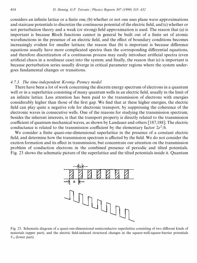
Fig. 23. Schematic diagram of a quasi-one-dimensional semiconductor superlattice consisting of two different kinds ofmaterials (upper part), and the electric field-induced structural changes in the square-well/square-barrier potentials»

0(lower part).

considers an infinite lattice or a finite one, (b) whether or not one uses plane wave approximationsand staircase potentials to discretize the continuous potential of the electric field, and (c) whether ornot perturbation theory and a weak (or strong) field approximation is used. The reason that (a) isimportant is because Bloch functions cannot in general be built out of a finite set of atomicwavefunctions in the presence of an electric field, and the effect of boundary conditions becomesincreasingly evident for smaller lattices; the reason that (b) is important is because differenceequations usually have more complicated spectra than the corresponding differential equations,and therefore discretization of a continuous process may easily introduce artificial spectra (evenartificial chaos in a nonlinear case) into the system; and finally, the reason that (c) is important isbecause perturbation series usually diverge in critical parameter regions where the system under-goes fundamental changes or transitions.

4.7.3. The time-independent Kronig—Penney modelThere have been a lot of work concerning the discrete energy spectrum of electrons in a quantum

well or in a superlattice consisting of many quantum wells in an electric field, usually in the limit ofan infinite lattice. Less attention has been paid to the transmission of electrons with energiesconsiderably higher than those of the first gap. We find that at these higher energies, the electricfield can play quite a negative role for electronic transport, by suppressing the coherence of theelectronic waves in consecutive wells. One of the reasons for studying the transmission spectrum,besides the inherent interests, is that the transport property is directly related to the transmissioncoefficient of quantum mechanical waves, as shown by Landauer and others [187,188]. The electricconductance is related to the transmission coefficient by the elementary factor 2e2/h.

We consider a finite quasi-one-dimensional superlattice in the presence of a constant electricfield, and determine how the transmission spectrum is affected by the field. We do not consider theexciton formation and its effect in transmission, but concentrate our attention on the transmissionproblem of conduction electrons in the combined presence of periodic and tilted potentials.Fig. 23 shows the schematic picture of the superlattice and the tilted potentials inside it. Quantum


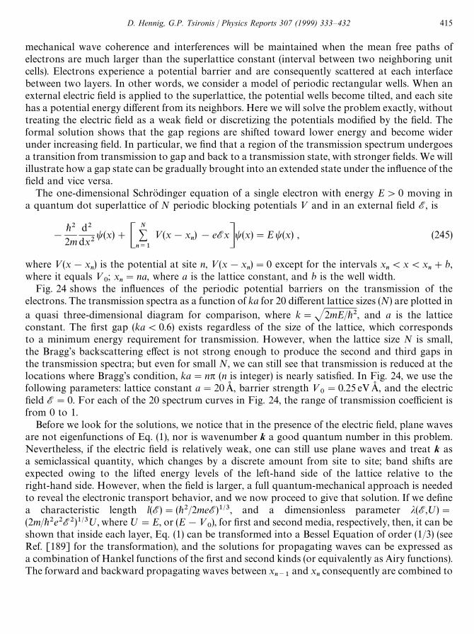
mechanical wave coherence and interferences will be maintained when the mean free paths ofelectrons are much larger than the superlattice constant (interval between two neighboring unitcells). Electrons experience a potential barrier and are consequently scattered at each interfacebetween two layers. In other words, we consider a model of periodic rectangular wells. When anexternal electric field is applied to the superlattice, the potential wells become tilted, and each sitehas a potential energy different from its neighbors. Here we will solve the problem exactly, withouttreating the electric field as a weak field or discretizing the potentials modified by the field. Theformal solution shows that the gap regions are shifted toward lower energy and become widerunder increasing field. In particular, we find that a region of the transmission spectrum undergoesa transition from transmission to gap and back to a transmission state, with stronger fields. We willillustrate how a gap state can be gradually brought into an extended state under the influence of thefield and vice versa.

The one-dimensional Schrodinger equation of a single electron with energy E'0 moving ina quantum dot superlattice of N periodic blocking potentials » and in an external field E, is

!

+2

2md2

dx2t(x)#C

N+n/1

»(x!xn)!eExDt(x)"Et(x) , (245)

where »(x!xn) is the potential at site n, »(x!x

n)"0 except for the intervals x

n(x(x

n#b,

where it equals »0; x

n"na, where a is the lattice constant, and b is the well width.

Fig. 24 shows the influences of the periodic potential barriers on the transmission of theelectrons. The transmission spectra as a function of ka for 20 different lattice sizes (N) are plotted ina quasi three-dimensional diagram for comparison, where k"J2mE/+2, and a is the latticeconstant. The first gap (ka(0.6) exists regardless of the size of the lattice, which correspondsto a minimum energy requirement for transmission. However, when the lattice size N is small,the Bragg’s backscattering effect is not strong enough to produce the second and third gaps inthe transmission spectra; but even for small N, we can still see that transmission is reduced at thelocations where Bragg’s condition, ka"np (n is integer) is nearly satisfied. In Fig. 24, we use thefollowing parameters: lattice constant a"20A_ , barrier strength »

0"0.25 eVA_ , and the electric

field E"0. For each of the 20 spectrum curves in Fig. 24, the range of transmission coefficient isfrom 0 to 1.

Before we look for the solutions, we notice that in the presence of the electric field, plane wavesare not eigenfunctions of Eq. (1), nor is wavenumber k a good quantum number in this problem.Nevertheless, if the electric field is relatively weak, one can still use plane waves and treat k asa semiclassical quantity, which changes by a discrete amount from site to site; band shifts areexpected owing to the lifted energy levels of the left-hand side of the lattice relative to theright-hand side. However, when the field is larger, a full quantum-mechanical approach is neededto reveal the electronic transport behavior, and we now proceed to give that solution. If we definea characteristic length l(E)"(+2/2meE)1@3, and a dimensionless parameter j(E,º)"(2m/+2e2E2)1@3º, where º"E, or (E!»

0), for first and second media, respectively, then, it can be

shown that inside each layer, Eq. (1) can be transformed into a Bessel Equation of order (1/3) (seeRef. [189] for the transformation), and the solutions for propagating waves can be expressed asa combination of Hankel functions of the first and second kinds (or equivalently as Airy functions).The forward and backward propagating waves between x

n~1and x

nconsequently are combined to


Fig. 24. Transmission coefficient vs. ka for 20 different lattice sizes. Gaps are produced by the coherent backscattering ofthe barriers on the wavefunctions of electrons. Parameters are given in the text.

give the following solution:

t(i)n(z)"A(i)

nz1@3H(1)

1@3(z)#B(i)

nz1@3H(2)

1@3(z) , (246)

where i"1, 2 indicating the first and second medium respectively, and

z(x,E,º)"23(j(E,º)#x/l(E))3@2

is the new dimensionless coordinate; (A(i)n, B(i)

n) are amplitude constants, which will be determined

solely by boundary conditions; and H(1,2)1@3

(z) are the Hankel functions of the first and second kind,respectively.

By differentiating Eq. (246) and using the recurrence relation of Bessel functions,

ddz

(zlJl(z))"zlJl~1(z) ,


where Jl(z) is any kind of Bessel function, we obtain dt/dx as follows:

dt(i)n

dx"

1l(E)

(32z2)

13[A(i)

nH(1)

~2@3(z)#B(i)

nH(2)

~2@3(z)] . (247)

Considering the continuity of t(xn) and dt/dx at the interfaces of different layers, a transfer matrix

between consecutive unit cells can be found. For simplicity in presentation, we only give specificresults for the d-function case: »"g

0a+

nd(x!x

n), where g

0is the average potential height in

a unit cell for the original lattice without field. The rectangular potentials are replaced byd-functions so that in each unit cell the particle is only scattered once. The unit-cell transfer matrixis shown as follows:

AA

n`1Bn`1B"A

1#wnh(1)n

/h(0)n

wnh(2)n

/h(0)n

!wnh(3)n

/h(0)n

1!wnh(1)n

/h(0)nBA

An

BnB , (248)

where wn"2ml/+2(3

2zn)~1@3g

0a, and all the h

n’s are products of Hankel functions of argument

zn"z(na,E, E), shown as follows: h(0)

n"H(2)

1@3(z

n)H(1)

~2@3(z

n)!H(1)

1@3(z

n)H(2)

~2@3(z

n), h(1)

n"

H(1)1@3

(zn)H(2)

1@3(z

n), h(2)

n"H(2)

1@3(z

n)2, and h(3)

n"H(1)

1@3(z

n)2. The analytical solutions of Eq. (1) are there-

fore completely determined:

AA

NBNB"¹

NAA

0B

0B"

1<n/N

MnA

A0

B0B , (249)

where A0,B

0are the initial amplitudes of the wavefunction, ¹

Nis the total transfer matrix between

x0

and xN, and M

nis the nth transfer matrix in Eq. (248). For a complete analysis, one should also

consider the transfer matrices connecting the field-free regions, x(x0

and x'xN, with the region

in the field, x0(x(x

n. The final transfer matrix is denoted as TN. The transmission coefficient

T is related to the final transfer matrix by

T"Ddet(TN)/(TN)22

D2 . (250)

4.7.4. Field-induced transmission spectral changesWe are interested in the case when the electronic wavelength is comparable with the superlattice

constant. Let k0"2p/a, and k

%"J2mE/+. We want to study the transmission problem for the

electrons with energies E, such that k%/k

0&0.1 to 10. For instance, if we take a"10 to 50A_ , and

E"0.01 to 1 eV, then we find that k%/k

0&0.1 to 4. To simplify our numerical results, we first define

two dimensionless quantities for eigenenergy and electric field strength. We define the dimension-less energy as EI "E/g

0, where again, g

0is the average barrier height in a unit cell; so if EI "1, it

means that the eigenenergy is at the average height of the barrier. We also define a dimensionlesselectric field as EI "eEa/g

0, where e is the electron’s charge, and a is the lattice constant, so that

EI can be seen as the relative potential drop within a cell caused by the electric field. We then canstudy how the transmission spectrum, as shown in Fig. 25, is changed by the electric field.

As we increase the field strength, we find the second gap (gap II) becomes wider, and shifts tothe left (lower value), as can be seen from Fig. 25b and c. The shift of the gap is not a surprise,because a similar result is expected from the semiclassical theory for conductivity. However, whenwe further increase the field strength, the original band structure collapses and gap II disappears;


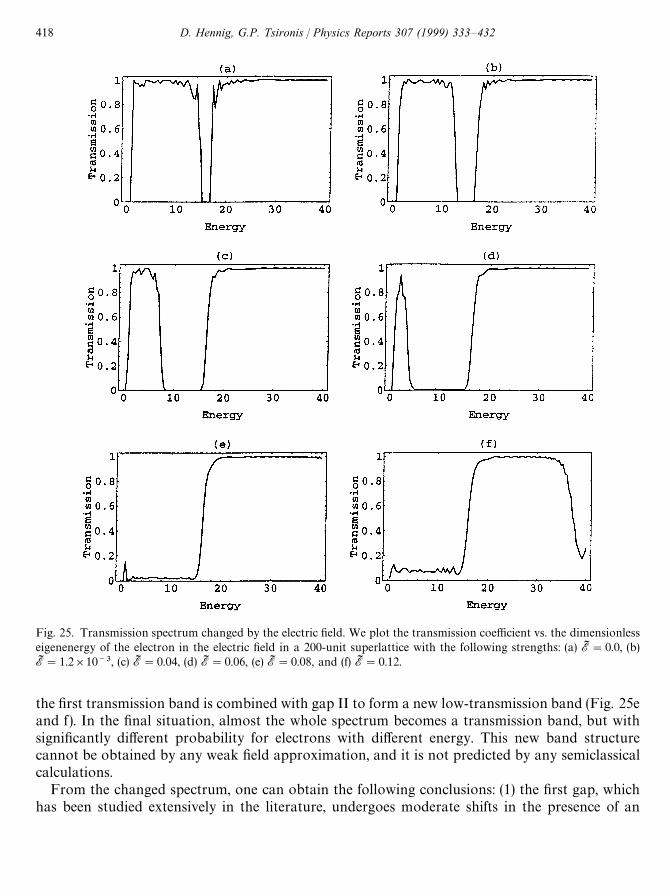
Fig. 25. Transmission spectrum changed by the electric field. We plot the transmission coefficient vs. the dimensionlesseigenenergy of the electron in the electric field in a 200-unit superlattice with the following strengths: (a) EI "0.0, (b)EI "1.2]10~3, (c) EI "0.04, (d) EI "0.06, (e) EI "0.08, and (f) EI "0.12.

the first transmission band is combined with gap II to form a new low-transmission band (Fig. 25eand f). In the final situation, almost the whole spectrum becomes a transmission band, but withsignificantly different probability for electrons with different energy. This new band structurecannot be obtained by any weak field approximation, and it is not predicted by any semiclassicalcalculations.

From the changed spectrum, one can obtain the following conclusions: (1) the first gap, whichhas been studied extensively in the literature, undergoes moderate shifts in the presence of an


Fig. 26. Electric field induced transmission and gap. Plot of transmission vs. the dimensionless electric field in a 200-unitsuperlattice with eigenenergies EI at left and right gap edges. (a) EI "15. An original gap point is brought to transmissionstatus by electric field; the threshold field is at about 0.06; (b) EI "12. An original transmission point is brought into gapregion by electric filed in the range of 0.02(EI (0.05, after that it returns to transmission state.

electric field, whereas the second gap is greatly expanded for moderate field strength; (2) an electronwith an eigenenergy initially at a transmission (conduction) state may become a gap electron in thefield and vice versa; (3) as the field strength is increased, the whole spectrum undergoes a drasticreconstruction, i.e. the first transmission band collapses, and then rises again, and merges with gapII to become a lower transmission band. These changes in transmission spectrum will affect theelectronic conductivity, and will result, in some cases, in oscillation between negative and positivedifferential resistances. We now study the transition processes at the transmission band edges.

Fig. 26 shows how the electric field affects the transmission coefficient of the electron at the leftand right gap edges; (a) for EI "15, a gap point when there is no electric field, is transformed intoa transmission point by the electric field when EI 50.06; (b) for EI "12, a transmission point whenthere is no field, is transformed into a gap state when 0.02(EI (0.05, and then returned toa transmission point for larger field strengths. In both cases after escaping from the gap, thetransmission coefficient increases smoothly over an interval of about 0.1, and then oscillates as thefield is increased.

4.7.5. Summary for the linear effectsWe have shown that the transmission spectrum of a superlattice may undergo large changes in

an electric field. Such changes will show up in electric conductivity of the superlattice. Similarchanges have been observed in other properties of semiconductor superlattices such as theelectro-optical effects [190,191] As in our present work, these effects are due to modification ofstates by the field and the resulting Stark—Wannier localization and intersubband resonance-induced delocalization [192]. We have given explicit results for a superlattice with 200 unit-cells(N"200), but similar results concerning the band shifting and the transitions between thetransmission and gap states exist for smaller lattices. However, when N is too small (in our casewhen N(25), Bragg backscattering from the blocking potentials will not be strong enough to


produce a gap, resulting in a lower transmission band sandwiched between two higher ones in thetransmission spectrum. In the presence of an electric field, the edges of the lower transmission bandis also shifted and the width is widened. For a stronger field, the distinction between the first twobands will disappear, similar to what is shown in Fig. 25f. Finally, we notice that the localizationbehavior in a disordered or quasiperiodic infinite system in the presence of an electric field has beenstudied extensively within the tight-binding model [193—195] and it has been found that localiza-tion either decays in real space by a power law or sometimes is totally eliminated by the field. Itwould be interesting to use the present model to study how disorder in a finite system would affectthe transmission property and hence the conductivity of the electrons in the electric field.

4.7.6. Multiple conductance in a nonlinear superlatticeIn this section we continue to use the Kronig—Penney model in the presence of an external

electric field and to study the nonlinear effects introduced by doped layers in a semiconductorsuperlattice. In particular, we will try to understand the experimentally observed multistability anddiscontinuity in the current-voltage characteristics of a doped semiconductor superlattice under anhomogeneous electric field. Nonlinearity in our model enters through the self-consistent potentialthat is used to describe the interaction of the electrons with charges in the doped layers. We showthat the process of Wannier—Stark localization is slowed down by the nonlinear effect in thedoped layers, and that the shrinking and destruction of minibands in the superlattice by thenonlinearity is responsible for the occurrence of discontinuity and multistability in the transport ofelectrons.

4.7.7. Multistability in electroconductanceThere have been considerable interests in the study of transmissions in a nonlinear medium for

both electrons and electromagnetic waves. It has been shown that under certain circumstancesnonlinearity can enhance transmission by a self-trapped mechanism and by producing andpropagating soliton-like waves in the nonlinear media [141,170]. The dynamics for the transmis-sions is determined by an interplay of nonlinearity and the periodicity (or the lack of it) of thematerial. In the ballistic regime of semiconductor nanostructures, electric conductance has beenfound to be related with transmission probabilities of quantum tunneling by an elementary factorof 2e2/h for each quantum channel that connects the outgoing waves with the incident waves[187,188].

Optical switching and multistability in nonlinear periodic structures have been analyzed exten-sively and observed in experiments since the work of Winful et al. [95,113,196,197]. Electric fieldinduced Stark ladder effect, Wannier—Stark localization and the electro-optical properties anddevice applications in the semiconductor superlattices (SL), such as GaAs/AlGaAs, have beenstudied extensively in recent years [181—186,198]. The quantum wave effect becomes significant insuch a system because the wavelengths of electrons in it are in the same order of magnitude as thesuperlattice constant. Recently, there have been renewed interests in the study of the multistabilityand discontinuity in the current—voltage (I—») diagram of doped semiconductor superlattices, boththeoretically [199,200] and experimentally [201]. It has been shown that the formation of chargedomains in a superlattice is the reason for multistability in electroconductance. In this section, wepresent a theoretical analysis and numerical calculations by using a simple model with techniquesof self-consistent potentials, to study the electronic transport in a SL. We demonstrate from


a fundamental quantum mechanical point of view how multistability and switching behaviorsoccur in a nonlinear discrete system.

4.7.8. A model with self-consistent potentialsThe wave functions of electrons in a superlattice must obey the Pauli’s principle. For simplicity,

we assume a decoupling between the longitudinal and transverse degrees of freedom to make theproblem one-dimensional. The nonlinearity arises from the self-consistent potentials [202] produc-ed by the accumulation of charges in the doped layers. The superlattice we consider here consists ofsquare-well/square-barrier semiconductor heterostructures, which is a common model represent-ing the mismatch in the minibands between two component materials of the superlattice. Weassume that the doped layers are located in the quantum barriers. Following Ref. [202], in theabsence of an external field, we write the self-consistent Schrodinger equation for t(x, t):

i+t

t(x, t)"C!+2

2m2

x2#»(x)#P¼(t, t@;x,x@)Dt(x@, t@)D2dt@dx@Dt(x, t), (251)

where »(x) is the periodic lattice potentials. We are interested in the time-independent solutions,t(x, t)"t(x) expMiutN. In such a case, the kernel is also assumed to be time-independent, and theintegral part in Eq. (251) is proportional to the density of charges in the doped layers. If the size ofthese regions is much smaller than the spatial variations of t(x), the integral part of Eq. (251) can bereplaced by the summation of the average contributions of the localized charges inside the wells:+¼M Dt(x

n)D2Dx

n; the average kernel in the well, ¼M , is proportional to e2n

%/C, where e is the electron

charge, n%

is the charge density in the doped layer and C is the capacitance of that layer. Forsimplicity, we assume that we have very thin doped layers, and use the d-function type of nonlinearbarriers to represent the self-consistent potentials; this is an approximation which makes it mucheasier to obtain an exact solution for this model. The integral in Eq. (251) is hence replaced by thefollowing summation, +wDt(x)D2d(x!x

n), where w is proportional to ¼M .

When an external electric field is applied along the growth axis of the superlattice, the mostfundamental change that the field makes is the breaking of the translational symmetry. The energylevels of neighboring wells are misaligned, which results in the Wannier—Stark localization owingto the turning-off of the resonant tunneling between consecutive wells, shifted absorption edges[198] and widened gap regions in the transmission spectrum [172]. The time-independentSchrodinger equation for the electron in an external electric field E, with energy E, and approach-ing a sample of N periodic potential barriers is

!

+2

2md2

dx2t(x)#C

N+n/1

g(DtD2)d(x!xn)!eExDt(x)"Et(x) , (252)

where g(DtD2)"p(g0#g

2Dt(x)D2), p is the potential strength; g

0and g

2are the weight factor

(pg2"w), representing the linear and self-consistent nonlinear potentials respectively; x

n"na,

where a is the lattice constant. Eq. (252) is very similar to Eq. (245), except that the barrier’spotential now contains a nonlinear term, the strength of which is proportional to the localprobability amplitude. As in Section 4.7.3, we define a characteristic length l(E)"(+2/2meE)1@3, anda dimensionless parameter j(E)"(2m/+2e2E2)1@3E then, it could be shown that between twoconsecutive d-function scatters, Eq. (252) can be transformed into a Bessel equation of order (1/3)


[172], and the solutions for propagating waves can be expressed as a combination of Hankelfunctions of the first and second kinds. The wave functions between x

n~1and x

nconsequently are

given as follows:

tn(z)"A

nz1@3H(1)

1@3(z)#B

nz1@3H(2)

1@3(z) , (253)

where z(x,E)"23j3@2(E)(1#x/j(E)l(E))3@2, is the new dimensionless coordinate; (A

n,B

n) are ampli-

tude constants, which will be determined later by boundary conditions; and H(1,2)1@3

(z) are the Hankelfunctions of the first and second kinds, respectively.

4.7.9. Multistability and multi-valued conductanceThere is a significant difference in the wave functions of a linear lattice and a nonlinear one. For

a linear lattice, g in Eq. (252) is a constant; the superposition principle holds for the waves in entirelattice. However, the same could not be said about a nonlinear lattice. It is possible that electronswith the same incident wave magnitude DA

0D, may not necessarily give the same output ¹, the

transmission coefficient of the sample.We calculate the transmission of electrons in a SL in the presence of an external electric field E,

and use Landauer’s formula to obtain the corresponding conductance. In Fig. 27, we show thetransmission coefficient ¹ (Fig. 27a) and the electric conductance G (Fig. 27b) as a function of thefield strength E for various values of g

2. In the linear case (g

2"0) and for a moderate electric field,

the wave-function of the electrons inside each quantum well is localized (W—S localization) and thetransmission is reduced due to the field induced reduction of the resonant tunneling betweenadjacent wells. As the electric field increases, the electrostatic potential energy of the electrons ineach QW is enhanced by the amount of eaE; if this value becomes comparable to DE

g, the energy

gap between two minibands, enhancement in transmission is expected because of the intersubbandresonant tunneling [192]. In the case of many minibands this process of enhanced transmissionrepeats itself also at higher field values resulting in the oscillatory pattern of the continuous curvesin Fig. 27. This oscillatory behavior is a manifestation of the competition between W—S localiza-tion and the intersubband resonance-induced delocalization. We note that the delocalization effectis completely absent from a single band model. The effects of W—S localization and the intersub-band resonance-induced delocalization can be observed through photon absorption and lumines-cence [181,182,192].

In the case of weak nonlinearity (g2"0.05 in Fig. 27), the oscillatory behavior of transmission

coefficient and conductance in the field remains similar to the linear case. However, the left andright sides of each peak becomes asymmetric, which means (a) the W—S localization process isslowed down in the presence of nonlinearity in the doped layers, as shown by the smaller slopes ofthe increasing curves in Fig. 27; and (b) the widths of the minibands shrink in the presence ofmoderate nonlinearity, so that the intersubband resonances occur in a narrower range of fieldvalues, resulting in the rapid drop after ¹ or G reaches a peak value. Finally, drastic changes areobserved in the case of strong nonlinearity (g

2"0.25 in Fig. 27). We notice that W—S localization

process is further slowed down in a increasing field, whereas the minibands structure is totallydestroyed by the nonlinearity, resulting in abrupt changes in transmission and conductance,including the occurrences of discontinuity and multistability. In Fig. 27, we use a"20A_ , N"40,and E"0.32 eV (this energy is roughly at the center of the second miniband of the linear model).For the barrier strength, we use p"2.0 eVA_ ; g

2"0.05, and 0.25, respectively, with g

0"1.0!g

2.


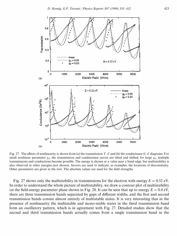
Fig. 27. The effects of nonlinearity is shown from (a) the transmission ¹—E and (b) the conductance G—E diagrams. Forsmall nonlinear parameter g

2, the transmission and conductance curves are tilted and shifted; for large g

2, multiple

transmissions and conductions become possible. The energy is chosen at a value near a band edge, but multistability isalso observed at other energies (not shown). Arrows are used to indicate, as examples, the locations of discontinuity.Other parameters are given in the text. The absolute values are used for the field strengths.

Fig. 27 shows only the multistability in transmissions for the electron with energy E"0.32 eV.In order to understand the whole picture of multistability, we draw a contour plot of multistabilityon the field-energy parameter plane shown in Fig. 28. It can be seen that up to energy E"0.4 eV,there are three transmission bands separated by gaps of different widths, and the first and secondtransmission bands consist almost entirely of multistable states. It is very interesting that in thepresence of nonlinearity the multistable and mono-stable states in the third transmission bandform an oscillatory pattern, which is in agreement with Fig. 27. Detailed studies show that thesecond and third transmission bands actually comes from a single transmission band in the


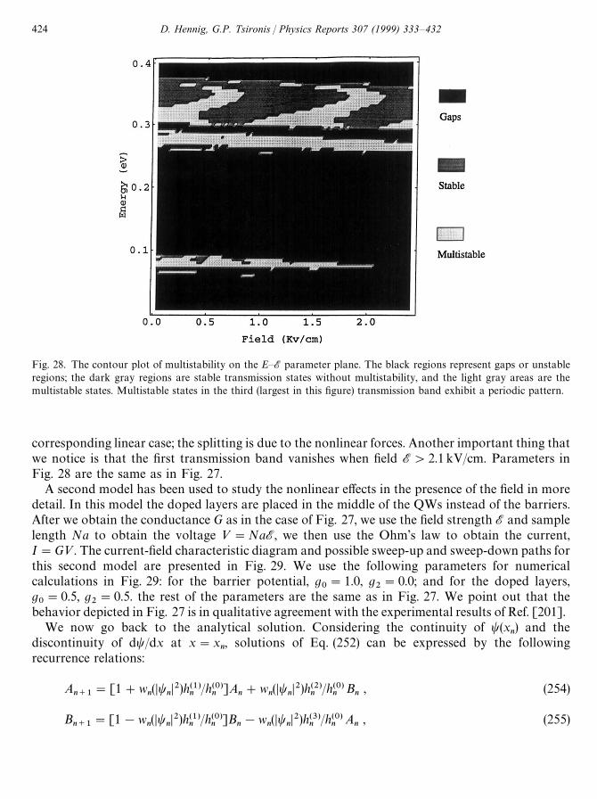
Fig. 28. The contour plot of multistability on the E—E parameter plane. The black regions represent gaps or unstableregions; the dark gray regions are stable transmission states without multistability, and the light gray areas are themultistable states. Multistable states in the third (largest in this figure) transmission band exhibit a periodic pattern.

corresponding linear case; the splitting is due to the nonlinear forces. Another important thing thatwe notice is that the first transmission band vanishes when field E'2.1 kV/cm. Parameters inFig. 28 are the same as in Fig. 27.

A second model has been used to study the nonlinear effects in the presence of the field in moredetail. In this model the doped layers are placed in the middle of the QWs instead of the barriers.After we obtain the conductance G as in the case of Fig. 27, we use the field strength E and samplelength Na to obtain the voltage »"NaE, we then use the Ohm’s law to obtain the current,I"G». The current-field characteristic diagram and possible sweep-up and sweep-down paths forthis second model are presented in Fig. 29. We use the following parameters for numericalcalculations in Fig. 29: for the barrier potential, g

0"1.0, g

2"0.0; and for the doped layers,

g0"0.5, g

2"0.5. the rest of the parameters are the same as in Fig. 27. We point out that the

behavior depicted in Fig. 27 is in qualitative agreement with the experimental results of Ref. [201].We now go back to the analytical solution. Considering the continuity of t(x

n) and the

discontinuity of dt/dx at x"xn, solutions of Eq. (252) can be expressed by the following

recurrence relations:

An`1

"[1#wn(Dt

nD2)h(1)

n/h(0)

n]A

n#w

n(Dt

nD2)h(2)

n/h(0)

nBn

, (254)

Bn`1

"[1!wn(Dt

nD2)h(1)

n/h(0)

n]B

n!w

n(Dt

nD2)h(3)

n/h(0)

nA

n, (255)


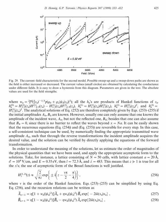
Fig. 29. The current—field characteristic for the second model. Possible sweep-up and a sweep-down paths are shown asthe field is either increased or decreased. The current values (small circles) are obtained by calculating the conductanceunder different fields. It is easy to draw a hysteresis from this diagram. Parameters are given in the text. The absolutevalues are used for the field strengths.

where wn"2ml+2 (3

2zn)~1@3p(g

0#g

2Dt

n(z

n)D2); all the h

n’s are products of Hankel functions of z

n.

h(0)n"H(2)

1@3(z

n)H(1)

~2@3(z

n)!H(1)

1@3(z

n)H(2)

~2@3(z

n), h(1)

n"H(1)

1@3(z

n)H(2)

1@3(z

n), h(2)

n"H(2)

1@3(z

n)2, and h(3)

n"

H(1)1@3

(zn)2. The analytical solutions of Eq. (252) are therefore completely given by Eqs. (253)—(255) if

the initial amplitudes A0, B

0are known. However, usually one can only assume that one knows the

amplitude of the incident wave, A0, but not the reflected one, B

0; besides that one can also assume

that BN"0, since there is no barrier to reflect the waves beyond x"Na. It can be easily shown

that the recurrence equations (Eq. (254)) and (Eq. (255)) are reversible for every step. In this case,a self-consistent technique can be used, by numerically finding the appropriate transmitted waveamplitude A

N, such that through the reverse transformations the incident amplitude acquires the

desired value, and the solution can be verified by directly applying the equations of the forwardtransformation.

In order to understand the meaning of the solutions, let us estimate the order of magnitudes ofthe physical quantities that we have been used, and apply the appropriate asymptotic form to thesolutions. Take, for instance, a lattice consisting of N"50 cells, with lattice constant a"20A_ ,E"104V/cm, and E"0.35 eV, then l"72.3A_ , and j"483. This means that z<1 is true for allthe x’s; the use of asymptotic form of the Bessel functions is well justified.

H(1,2)l (z)+S2pz

expG$iAz!lp2!

p4BH , (256)

where l is the order of the Hankel function. Eqs. (253)—(255) can be simplified by using Eq.Eq. (256), and the recursion relations can be written as

AIn`1

"g[1#wn(Dt

nD2)]AI

n#gw

n(Dt

nD2)BI

nexpM!2ik(x

n)x

nN , (257)

BIn`1

"g[1!wn(Dt

nD2)]BI

n!gw

n(Dt

nD2)AI

nexpM2ik(x

n)x

nN , (258)


where g"(zn/z

n`1)~1@6, AI

n"J(2/n)z~1@6

nA

nexp(ih), and BI

n"J(2/n)z~1@6

nB

nexp(!ih), with

h"(2/3)j3@2!(5/12)p. The electron is gaining kinetic energy in the field, and its “wavenumber”k(x) is an increasing function of x, given by

k(x)"k0C1#

14j~3@2k

0x2!

124

j~3k20x3#2D ,

where k0"J2mE/+. The asymptotic solution then can be seen as a modified plane wave.

tn(x)"(z

n/z)1@6AI

ne*k(x)x#(z

n/z)1@6BI

ne~*k(x)x . (259)

The asymptotic relations are useful in that it helps to illustrate the physical processes, and havebeen found to be quite reliable for the parameters that we have used. Nevertheless, all the physicalquantities of our interests can be calculated directly from Eqs. (253)—(255).

We have demonstrated that the occurrence of multistability and discontinuity in the transportprocesses of electrons can be explained by introducing the self-consistent potentials to represent thenonlinear space charge effects in the doped semiconductor layers. We use a simple model in whichthe doped layers are assumed to be ultrathin and provide nonlinear impacts on the wave packagesof the electrons. One of the advantages of this model is that a fully quantum-mechanical treatmentcan be applied without using an effective Hamiltonian. Comparing with the tight-binding model,which is good only for weakly coupled QWs heterostructure, our model inherently creates a seriesof minibands (multiple conduction subbands structure), and the interwell coupling of the wavefunctions of all the QWs is fully considered in our algorithm. These couplings are responsible fortunneling and transmission of electrons, and become increasingly important in a superlatticefabricated with thinner barriers. This model can be easily modified to study other heterostructuresin an electric field, such as a SL consisting of alternative n and p-doped layers and the modulationsmade by impurity and disorder.

5. Conclusions

We have demonstrated that simple nonlinear lattice systems such as the ones formed through thediscrete nonlinear Schrodinger equation and its generalizations can be used to model severalphysical circumstances ranging from polaron and soliton like problems to nonlinear electrical andoptical problems. The main virtue of DNLS-like models is their simplicity, viz. with relativelysimple formalism one can describe complicated phenomena. In many cases, such as the one of thenonlinear photonic band gap systems, one can bypass completely the complexity of the realproblem while sacrificing only in the quantitative aspects of the results.

In this review we addressed primarily transfer properties of nonlinear lattices. The stationarylattice problem becomes then equivalent to an effective dynamical system described througha nonlinear map whose dynamics corresponds to discrete propagation on the lattice. The mapproperties are then investigated though the use of standard analytical and numerical techniques.The map associate with the DNLS-AL equation shows rich behavior and different regimes


depending on the relative strengths of the “integrable” to the “non-integrable” nonlinear terms. Wesaw that the integrable map regime can be extended to substantial values of the nonlinearitycoefficient of the local nonlinear term. The nonintegrable regime is characterized by sensitivity inthe initial condition dependence leading, in the lattice problem, to nonpropagating stationarystates. The latter do not contribute in the lattice transfer properties.

One interesting application of nonlinear lattices is in one dimensional nonlinear photonic bandgap systems. In these systems there is an interplay between nonlinearity and the presence of gaps inthe linear band leading to selective amplitude dependent transmission, or switching. We showedsome of these properties through a straightforward many band generalization of DNLS, viz.a nonlinear Kronig—Penney model with delta functions. Since in proper variables this systemcorresponds to a DNLS equation with wavevector dependent nonlinearity coefficient, we used themap approach to study its transmission properties. We also addressed transfer properties in thepresence of external fields, targeting semiconductor superlattice applications. We saw that severalof the conclusions arrived through the map method can represent qualitatively results obtainedexperimentally.

Acknowledgements

We thank our collaborators Ning Sun, Mario Molina, Bill Deering, Helmut Gabriel, and KimRasmussen for exciting and stimulating discussion over the last several years. This work waspartially supported by the European Union under the Human Capital and Mobility programERB-CHRX-CT-930331. One of the authors (D.H.) gratefully acknowledges the warm hospitalityof the Research Center of Crete, Greece and support from the Deutsche Forschungsgemeinschaftvia SFB 337.

References

[1] J.C. Eilbeck, P.S. Lomdahl, A.C. Scott, Physica D 16 (1985) 318.[2] V.M. Kenkre, D.K. Campbell, Phys. Rev. B 34 (1986) 4959.[3] T. Holstein, Ann. Phys. (N.Y.) 8 (1959) 325.[4] A.S. Davydov, N.I. Kislukha, Phys. Status. Solidi B 59 (1973) 465.[5] A.S. Davydov, J. Theor. Biol. 38 (1973) 559.[6] A.S. Davydov, N.I. Kislukha, Sov. Phys. JETP 44 (1976) 571.[7] A.S. Davydov, Sov. Phys. Rev. B 25 (1982) 898.[8] J.C. Eilbeck, P.S. Lomdahl, A.C. Scott, Phys. Rev. B 30 (1984) 4703.[9] A.C. Scott, P.S. Lomdahl, J.C. Eilbeck, Chem. Phys. Lett. 113 (1985) 29.

[10] A.C. Scott, J.C. Eilbeck, Chem. Phys. Lett. 132 (1986) 23.[11] V.M. Kenkre, G.P. Tsironis, D.K. Campbell, in: A.R. Bishop et al. (Eds.), Nonlinearity in Condensed Matter,

Springer, Berlin, 1987.[12] G.P. Tsironis, V.M. Kenkre, Phys. Lett. A 127 (1989) 209.[13] V.M. Kenkre, G.P. Tsironis, Phys. Rev. B 35 (1987) 1473.[14] V.M. Kenkre, G.P. Tsironis, Chem. Phys. 128 (1989) 219.[15] D. Hennig, B. Esser, Z. Phys. B 88 (1992) 231.[16] M.J. Ablowitz, J.F. Ladik, J. Math. Phys. 17 (1976) 1011.


[17] M. Salerno, Phys. Rev. A 46 (1992) 6856.[18] D. Cai, A.R. Bishop, N. Gronbech-Jensen, Phys. Rev. Lett. 72 (1994) 591.[19] S.M. Jensen, IEEE J. Quant. Electron. QE-18 (10) (1982) 1580.[20] M.I. Molina, G.P. Tsironis, Physica D 65 (1993) 267.[21] A.A. Maier, Sov. J. Quantum Electron. 14 (1984) 101.[22] P.N. Buthcher, D. Cotter, The Elements of Nonlinear Optics, Cambridge Univ. Press, Cambridge, 1990.[23] P. Marquie, J.M. Bilbault, Remoissenet, Phys. Rev. E 51 (1995) 6127.[24] M. Toda, Theory of Nonlinear Lattices, Springer, Berlin, 1978.[25] R. Hirota, K. Suzuki, Proc. IEEE 61 (1973) 1483.[26] M. Remoissenet, Waves Called Solitons, Springer, Berlin, 1994.[27] V.I. Arnold, A. Avez, Ergodic Problems of Classical Mechanics, Benjamin, New York, 1968.[28] A.J. Lichtenberg, M.A. Liebermann, Regular and Stochastic Motion, Springer, New York, 1992.[29] J. Greene, R.S. MacKay, F. Vivaldi, M.J. Feigenbaum, Physica D 3 (1981) 468.[30] R.S. MacKay, Physica D 7 (1983) 283.[31] J.D. Meiss, Rev. Mod. Phys. 64 (1992) 795.[32] T.C. Bountis, Part. Accel. 19 (1986) 181.[33] R.H.G. Helleman, in: C. Horton, L. Reichl, V. Szebehely (Eds.), Long-time Predictions in Dynamics, Wiley-

Interscience, New York, 1983.[34] T. Chen et al., Phys. Rev. Lett. 68 (1991) 33.[35] T. Satogata et al., Phys. Rev. Lett. 68 (1991) 1838.[36] M. Kohomoto, L.P. Kadanoff, C. Tang, Phys. Rev. Lett. 50 (1983) 1870; M. Kohomoto, B. Sutherland, K. Iguchi,

Phys. Rev. Lett. 58 (1987) 2436.[37] G. Gumbs, M.K. Ali, Phys. Rev. Lett. 60 (1988) 1081; J. Phys. A 21 (1988) L517.[38] F. Wijnands, J. Phys. A 22 (1989) 3267.[39] J. Bellisard, B. Iochum, E. Scoppola, D. Testard, Commun. Math. Phys. 125 (1989) 527.[40] S. Aubry, G. Andre, Ann. Israel Phys. Soc. 3 (1980) 133.[41] S. Aubry, Physica D 7 (1983) 240.[42] S. Aubry, P.Y. LeDaeron, Physica D 8 (1983) 381.[43] J. Greene, J. Math. Phys. 20 (1979) 257.[44] V.I. Arnold, Mathematical Methods of Classical Mechanics, Springer, New York, 1978.[45] R. Devaney, Trans. Am. Math. Soc. 218 (1976) 89.[46] A.A. Vakhnenko, Yu.B. Gadidei, Theor. Math. Phys. 68 (1986) 873.[47] G.L. Wiersma, H.W. Capel, Physica A 142 (1987) 199; 149 (1988) 49, 75; Phys. Lett. A 124 (1987) 124.[48] M.L. Glaser, V.G. Papageorgiou, T.C. Bountis, SIAM J. Appl. Math. 49 (1989) 692.[49] T.R. Taha, M.J. Ablowitz, J. Comput. Phys. 55 (1984) 192 203.[50] B.M. Herbst, M.J. Ablowitz, Phys. Rev. Lett. 62 (1989) 2065.[51] C.G.J. Jacobi, see G. Birkhoff, Dynamical systems, Am. Math. Soc. Coll. Publ. vol. IX, American Mathematical

Society, Providence, RI, 1927.[52] G.R.W. Quispel, J.A.G. Roberts, C.J. Thompson, Physica D 34 (1989) 183.[53] G.R.W. Quispel, J.A.G. Roberts, C.J. Thompson, Phys. Lett. A 126 (1988) 419.[54] E.M. McMillan, in: W.E. Brittin, Odabasi (Eds.), Topics in Physics, Colorado Associated Univ. Press, Boulder,

1971, p. 219.[55] K.A. Ross, C.J. Thompson, Physica A 135 (1986) 551.[56] M.J. Ablowitz, P.A. Clarkson, Solitons, Nonlinear Evolution Equations and Inverse Scattering, Cambridge Univ.

Press, New York, 1991.[57] N. Finlayson, G.I. Stegeman, Appl. Phys. Lett. 56 (1990) 2276.[58] Y. Chen, A.W. Snyder, D.J. Mitchell, Electron. Lett. 26 (1990) 77.[59] A.C. Scott, Phys. Scr. 42 (1990) 14.[60] L. Bernstein, J.C. Eilbeck, A.C. Scott, Nonlinearity 3 (1990) 293.[61] J.C. Eilbeck, in: P.L. Christiansen, A.C. Scott (Eds.), Davydov’s Soliton Revisited, Plenum Press, New York,

1991.


[62] C. Schmidt-Hattenberger, U. Trutschel, F. Lederer, Opt. Lett. 16 (1991) 294.[63] M.I. Molina, G.P. Tsironis, Phys. Rev. A 46 (1992) 1124.[64] G.P. Tsironis, Phys. Lett. A 173 (1993) 381.[65] D. Hennig, Physica D 64 (1993) 121.[66] J.C. Eilbeck, G.P. Tsironis, S. Turitsyn, Phys. Scr. 52 (1995) 386.[67] M.I. Molina, W.D. Deering, G.P. Tsironis, Physica D 66 (1993) 135.[68] G.P. Tsironis, D. Hennig, N.G. Sun, unpublished.[69] Yu.S. Kivshar, M. Peyrard, Phys. Rev. A 46 (1992) 3198.[70] Ch. Claude, Yu.S. Kivshar, O. Kluth, K.H. Spatschek, Phys. Rev. B 47 (1993) 14 228.[71] Yu.S. Kivshar, M. Salerno, Phys. Rev. E 49 (1994) 3543.[72] M.H. Hays, C.D. Levermore, P.D. Miller, Physica D 79 (1994) 1.[73] V.V. Konotop, O.A. Chubykalo, L. Vazquez, Phys. Rev. E 48 (1993) 563.[74] D. Cai, A.R. Bishop, N. Gr+nbech-Jensen, M. Salerno, Phys. Rev. Lett. 74 (1995) 1186.[75] R. Scharf, A.R. Bishop, Phys. Rev. A 43 (1991) 6535.[76] D. Hennig, K.O. Rasmussen, G.P. Tsironis, H. Gabriel, Phys. Rev. E 52 (1995) 4628.[77] A.B. Aceves, C. De Angelis, A.R. Rubenchik, S.K. Turitsyn, Opt. Lett. 19 (1994) 329.[78] A.B. Aceves, C. De Angelis, S. Trillo, S. Wabnitz, Opt. Lett. 19 (1994) 332.[79] A.B. Aceves, C. De Angelis, T. Peschel, R. Muschall, F. Lederer, S. Trillo, S. Wabnitz, Phys. Rev. E 53 (1996)

1172.[80] D. Cai, A.R. Bishop, N. Gr+nbech-Jensen, Phys. Rev. E 53 (1996) 4131.[81] F. Delyon, Y.-E. Levy, B. Souillard, Phys. Rev. Lett. 57 (1986) 2010.[82] Yi Wan, C.M. Soukoulis, Phys. Rev. A 41 (1990) 800; Yi Wan, C.M. Soukoulis, in: A.R. Bishop, D.K. Campbell, S.

Pnevmatikos (Eds.), Disorder and Nonlinearity, Springer, Berlin, 1989, pp. 27—37.[83] D. Hennig, N.G. Sun, H. Gabriel, G.P. Tsironis, Phys. Rev. E 52 (1995).[84] H.A. Kramers, Physica 2 (1935) 483.[85] H.M. James, Phys. Rev. 76 (1949) 1602.[86] W. Kohn, Phys. Rev. 115 (1959) 809.[87] R.E. Borland, in: E. Lieb, D.C. Mattis (Eds.), Mathematical Physics in One Dimension, Academic Press, New

York, 1966.[88] D.R. Hofstadter, Phys. Rev. B 14 (1976) 2239.[89] R. Bellman, Introduction to Matrix Analysis, McGraw-Hill, New York, 1970.[90] V.I. Arnold, in: R.Z. Sagdeev (Ed.), Nonlinear and Turbulent Processes in Physics, Harwood, Chur, 1984,

p. 116.[91] I. Shimada, T. Nagashima, Prog. Theor. Phys. 61 (1979) 1605.[92] V.I. Oseledec, Trans. Mosc. Math. Soc. 19 (1968) 197.[93] G. Benettin, L. Galgani, J.M. Strelcyn, Phys. Rev. A 14 (1976) 22 338.[94] T. Bountis, Physica D 3 (1981) 577.[95] H.G. Winful, J.H. Marburger, E. Garmire, Appl. Phys. Lett. 35 (1979) 379.[96] L. Kahn, N.S. Almeida, D.L. Mills, Phys. Rev. B 37 (1988) 8072.[97] A.J. Sievers, S. Takeno, Phys. Rev. Lett. 61 (1988) 970.[98] J.B. Page, Phys. Rev. B 41 (1990) 7835.[99] S. Takeno, S. Homma, J. Phys. Soc. Japan 60 (1991) 731, 62 (1993) 835; S. Takeno, K. Hori, J. Phys. Soc. Japan 60

(1991) 947; S. Takeno, J. Phys. Soc. Japan 61 (1992) 2821; S.R. Bickham, S.A. Kiselev, A.J. Sievers, Phys. Rev. B 47(1993) 14206; K.W. Sandudsky, J.B. Page, K.E. Schmidt, Phys. Rev. B 46 (1992) 6161.

[100] T. Dauxois, M. Peyrard, C.R. Willis, Physica D 57 (1992) 267; Phys. Rev. E 48 (1993) 4768.[101] T. Dauxois, M. Peyrard, Phys. Rev. Lett. 70 (1993) 3935.[102] S. Flach, C.R. Willis, E. Olbrich, Phys. Rev. E 49 (1994) 836.[103] S. Flach, C.R. Willis, Phys. Rev. Lett. 72 (1994) 1777.[104] E.W. Laedke, K.H. Spatsckek, S.K. Turitsyn, Phys. Rev. Lett. 73 (1994) 1055.[105] S. Aubry, Physica D 71 (1994) 196.[106] S. Aubry, Physica D 86 (1995) 284.


[107] J. Coste, J. Peyrard, Phys. Rev. B 39 (1989) 13086; ibid 39 (1989) 13096.[108] J. Coste, J. Peyrard, Z. Phys. B 96 (1994) 111.[109] H.G. Winful, Appl. Phys. Lett. 46 (1985) 527.[110] W. Chen, D.L. Mills, Phys. Rev. B 35 (1986) 524.[111] W. Chen, D.L. Mills, Phys. Rev. Lett. 58 (1987) 160.[112] D.L. Mills, S.E. Trullinger, Phys. Rev. B 36 (1987) 947.[113] W. Chen, D.L. Mills, Phys. Rev. B 36 (1987) 6269.[114] Yu.S. Kivshar, Phys. Rev. Lett. 70 (1993) 3055.[115] D. Hennig, K.". Rasmussen, H. Gabriel, A. Bulow, Phys. Rev. E 54 (1996) 5788.[116] J. Guckenheimer, P. Holmes, Nonlinear Oscillations, Dynamical Systems, and Bifurcations of Vector Fields,

Springer, New York, 1983.[117] S. Aubry, G. Abramovici, Physica D 43 (1990) 199.[118] S. Aubry, Physica D 71 (1994) 196.[119] R.S. MacKay, S. Aubry, Nonlinearity 7 (1994) 1623.[120] P.C. Bressloff, Phys. Rev. Lett. 75 (1995) 962.[121] J.J.P. Veerman, F.M. Tangerman, Commun. Math. Phys. 139 (1991) 245.[122] R.S. MacKay, J.D. Meiss, Nonlinearity 5 (1992) 149.[123] C. Baesens, R.S. MacKay, Physica D 71 (1994) 372.[124] M.L. Glasser, V.G. Papageorgiou, T.C. Bountis, SIAM J. Appl. Math. 49 (1989) 692.[125] P.F. Byrd, M.D. Friedman, Handbook of Elliptic Integrals for Engineers and Scientists, Springer, New York,

1971.[126] G.D. Birkhoff, Acta Math. 43 (1920) 1.[127] E. Tabacman, Physica D 85 (1995) 548.[128] J. Moser, Commun. Pure, Appl. Math. 9 (1956) 673.[129] G.L. Da Silva Ritter, A.M. Ozorio de Almeida, R. Douady, Physica D 29 (1987) 181.[130] K. Furuya, A.M. Ozorio de Almeida, J. Phys. A: Math. Gen. 20 (1987) 6211.[131] V.M. Eleonskii, N.E. Kulagin, N.S. Novozhilova, V.P. Silin, Theor. Math. Phys. 60 (1984) 395.[132] D. Hennig, submitted (1997).[133] Yu.S. Kivshar, D.K. Campbell, Phys. Rev. E 48 (1993) 3077.[134] R. de L. Kronig, W.G. Penney, Proc. R. Soc. London, Ser. A 130 (1931) 499.[135] See, e.g., E. Lieb, D.C. Mattis, Mathematical Physics in One Dimension, Academic Press, New York, 1966; J.

Kollar, A. Suto8 , Phys. Lett. A 117 (1986) 203; F. Dominguez-Adame, A. Sanchez, Phys. Lett. A 159 (1991) 135; A.Sanchez, E. Macia, F. Dominguez-Adame, Phys. Rev. B 49 (1994) 147.

[136] M. Jaros, Physics and Applications of Semiconductor Microstructures, Clarendon Press, Oxford, 1989; E. Tuncel,L. Pavesi, Phil. Mag. B 65 (1992) 213.

[137] Y. Tanaka, M. Tsukada, Phys. Rev. B 40 (1989) 4482.[138] G.J. Clerk, B.H.J. Kellar, Phys. Rev. C 41 (1990) 1198.[139] P. Hawrylak, M. Grabowski, P. Wilson, Phys. Rev. B 40 (1989) 6398.[140] M. Grabowski, P. Hawrylak, Phys. Rev. B 41 (1990) 5783.[141] D. Hennig, H. Gabriel, G.P. Tsironis, M.I. Molina, Appl. Phys. Lett. 64 (1994) 2934.[142] D. Hennig, G.P. Tsironis, M.I. Molina, H. Gabriel, Phys. Lett. A 190 (1994) 259.[143] J. Bellisard, A. Formoso, R. Lima, D. Testard, Phys. Rev. B 26 (1982) 3024.[144] D. Wurtz, M.P. Soerensen, T. Schneider, Helv. Physica Acta 61 (1988) 345.[145] P. Erdos, R.C. Herndon, Adv. Phys. 31 (1982) 65.[146] M.Ya. Azbel, Phys. Rev. Lett. 43 (1979) 1954.[147] J.B. Sokoloff, J.V. Jose, Phys. Rev. Lett. 49 (1982) 334.[148] R. Knapp, G. Papanicolaou, B. White, in: A.R. Bishop, D.K. Campbell, S. Pnevmatikos (Eds.), Disorder and

Nonlinearity, Springer, Berlin, 1989, pp. 2—26.[149] S. John, Phys. Rev. Lett. 53 (1984) 2169.[150] S. John, Phys. Rev. Lett. 58 (1987) 2486.[151] E. Yablonovitch, Phys. Rev. Lett. 58 (1987) 2059.


[152] S. John, R. Rangarajan, Phys. Rev. B 38 (1988) 10 101.[153] K.M. Ho, C.T. Chan, C.M. Soukoulis, Phys. Rev. Lett. 65 (1990) 3152.[154] M. Sigalas, C.M. Soukoulis, E.N. Economou, C.T. Chan, K.M. Ho, Phys. Rev. B 48 (1993) 121.[155] G. Jona-Lasinio, C. Presilla, F. Capasso, Phys. Rev. Lett. 68 (1992) 2269.[156] M.I. Molina, G.P. Tsironis, Phys. Rev. Lett. 73 (1994) 464.[157] M.I. Molina, W.D. Deering, G.P. Tsironis, Physica D 66 (1993) 135.[158] D. Schectman, I. Blech, D. Gratias, J.W. Cahn, Phys. Rev. Lett. 53 (1984) 1951.[159] W. Gellermann, M. Kohmoto, B. Sutherland, P.C. Taylor, Phys. Rev. Lett. 72 (1994) 633.[160] R. Merlin, K. Bajema, R. Clarke, F.Y. Juang, P.K. Bhattacharya, Phys. Rev. Lett. 55 (1985) 1768.[161] B. Sutherland, Phys. Rev. B 34 (1986) 3904.[162] M. Kohmoto, B. Sutherland, C. Tang, Phys. Rev. B 35 (1987) 1020.[163] H. Hiramoto, M. Kohmoto, Int. J. Mod. Phys. B 6 (1992) 281.[164] S. Ostlund, R. Pandit, D. Rand, J. Schellnhuber, E. Siggia, Phys. Rev. Lett. 50 (1983) 1873.[165] P. Hu, C.S. Ting, Phys. Rev. B 34 (1986) 8331.[166] L.M. Kahn, K. Huang, D.L. Mills, Phys. Rev. B 39 (1989) 12 449.[167] S.D. Gupta, D.S. Ray, Phys. Rev. B 38 (1988) 3628; 40 (1989) 10 604; 41 (1990) 8047.[168] M. Johansson, R. Riklund, Phys. Rev. B 49 (1994) 6587; 52 (1995) 231.[169] H. Hiramoto, J. Phys. Japan 59 (1990) 811.[170] N. Sun, D. Hennig, M. Molina, G. Tsironis, J. Phys.: Condens. Matter 6 (1994) 7741.[171] G. Nenciu, Rev. Mod. Phys. 63 (1993) 91.[172] Ning G. Sun, Daiqing Yuan, W.D. Deering, Phys. Rev. B. 51 (1995) 4641.[173] N.G. Sun, G.P. Tsironis, Phys. Rev. B 51 (1995) 11 221.[174] G.H. Wannier, Phys. Rev. 117 (1960) 432.[175] J. Zak, Phys. Rev. Lett. 20 (1968) 1477.[176] G.H. Wannier, Phys. Rev. 181 (1969) 1364; J. Zak, Phys. Rev. 181 (1969) 1366.[177] J.R. Banavar, D.D. Coon, Phys. Rev. B 17 (1978) 3744.[178] D. Emin, C.F. Hart, Phys. Rev. B 36 (1987) 7353.[179] G. Bastard, J.A. Brum, R. Ferreira, Electronic states in semiconductor Heterostructures, in: H. Ehrenreich,

D. Turnbull (Eds.), Solid State Physics, vol. 44, Academic Press, New York, 1991.[180] L. Esaki, R. Tsu, IBM J. Res. Develop. 14 (1970) 61.[181] D.A.B. Miller, D.S. Chemla, T.C. Damen, A.C. Gossard, W. Wiegman, T.H. Wood, C.A. Burrus, Phys. Rev. B 32

(1985) 1043.[182] E.E. Mendez, F. Agullo-Rueda, J.M. Hong, Phys. Rev. Lett. 60 (1988) 2426.[183] F. Agullo-Rueda, E.E. Mendez, H. Ohno, J.M. Hong, Phys. Rev. B 42 (1990) 1470.[184] M.M. Dignam, J.E. Sipe, Phys. Rev. Lett. 64 (1990) 1797.[185] R.H. Yu, Phys. Rev. B 49 (1994) 4673.[186] E.E. Mendez, in: F. Henneberger, S. Schmitt-Rink, E.O. Gobel (Eds.), Optics of Semiconductor Nanostructures,

Akademie Verlag, Berlin, 1993.[187] R. Landauer, Phil. Mag. 21 (1970) 863; J. Phys.: Condens. Matter 1 (1989) 8099.[188] P.W. Anderson, D.J. Thouless, E. Abrahams, D.S. Fisher, Phys. Rev. B 22 (1980) 3519.[189] S. Flugge, Practical Quantum Mechanics, vol. 1, Springer, Berlin, 1971.[190] J. Bleuse, G. Bastard, P. Voisin, Phys. Rev. Lett. 60 (1988) 220.[191] I. Bar-Joseph, K.W. Goossen, J.M. Kou, R.F. Kopt, D.A.B. Miller, D.S. Chemla, App. Phys. Lett. 55 (1989)

340.[192] H. Schneider, H.T. Grahn, K.V. Klitzing, K. Ploog, Phys. Rev. Lett. 65 (1990) 2720.[193] C.M. Soukoulis, J.V. Jose, E.N. Economou, P. Sheng, Phys. Rev. Lett. 50 (1983) 764.[194] F. Delyon, B. Simon, B. Souillard, Phys. Rev. Lett. 52 (1984) 2187.[195] K. Niizeki, A. Matsumura, Phys. Rev. B 48 (1993) 4126.[196] C.J. Herbert, M.S. Malcuit, Opt. Lett. 18 (1993) 1783.[197] J. He, M. Cada, M.A. Dupertuis, D. Martin, F. Morier-Genoud, C. Rolland, A. SpringThorpe, Appl. Phys. Lett. 63

(1993) 866; B. Acklin, M. Cada, J. He, M.A. Dupertuis, Appl. Phys. Lett. 63 (1993) 2177.


[198] Paul Voisin, Surf. Sci. 288 (1990) 74.[199] B. Laikhtman, D. Miller, Phys. Rev. B 48 (1993) 5395.[200] F. Prengel, A. Wacker, E. Scholl, Phys. Rev. B 50 (1994) 1705.[201] J. Kastrup, H.T. Grahn, K. Ploog, F. Prengel, A. Wacker, E. Scholl, Appl. Phys. Lett. 65 (1994) 1808.[202] C. Presilla, G. Jona-Lasinio, F. Capasso, Phys. Rev. B 43 (1991) 5200.


wave transmission in nonlinear lattices · 3.5. normal form computation of the homoclinic tangle...

Documents