homoclinic orbits of the fitzhugh-nagumo equation: the ...math.cornell.edu/~gucken/pdf/fhnc.pdf ·...

DISCRETE AND CONTINUOUS doi:10.3934/dcdss.2009.2.851DYNAMICAL SYSTEMS SERIES SVolume 2, Number 4, December 2009 pp. 851–872

HOMOCLINIC ORBITS OF THE FITZHUGH-NAGUMO

EQUATION: THE SINGULAR-LIMIT

John Guckenheimer

Mathematics DepartmentCornell University

Ithaca, NY 14853, USA

Christian Kuehn

Center for Applied MathematicsCornell University

Ithaca, NY 14853, USA

Abstract. The FitzHugh-Nagumo equation has been investigated with a widearray of different methods in the last three decades. Recently a version ofthe equations with an applied current was analyzed by Champneys, Kirk,Knobloch, Oldeman and Sneyd [5] using numerical continuation methods.They obtained a complicated bifurcation diagram in parameter space featuringa C-shaped curve of homoclinic bifurcations and a U-shaped curve of Hopf bi-furcations. We use techniques from multiple time-scale dynamics to understandthe structures of this bifurcation diagram based on geometric singular pertur-bation analysis of the FitzHugh-Nagumo equation. Numerical and analyticaltechniques show that if the ratio of the time-scales in the FitzHugh-Nagumoequation tends to zero, then our singular limit analysis correctly represents theobserved CU-structure. Geometric insight from the analysis can even be used

to compute bifurcation curves which are inaccessible via continuation methods.The results of our analysis are summarized in a singular bifurcation diagram.

1. Introduction.

1.1. Fast-Slow Systems. Fast-slow systems of ordinary differential equations(ODEs) have the general form:

ǫx = ǫdx

dτ= f(x, y, ǫ) (1)

y =dy

dτ= g(x, y, ǫ)

where x ∈ Rm, y ∈ R

n and 0 ≤ ǫ ≪ 1 represents the ratio of time scales. The func-tions f and g are assumed to be sufficiently smooth. In the singular limit ǫ → 0 thevector field (1) becomes a differential-algebraic equation. The algebraic constraintf = 0 defines the critical manifold C0 = {(x, y) ∈ R

m ×Rn : f(x, y, 0) = 0}. Where

Dxf(p) is nonsingular, the implicit function theorem implies that there exists a maph(x) = y parametrizing C0 as a graph. This yields the implicitly defined vector field

2000 Mathematics Subject Classification. Primary: 34E13, 34E15, 37G20, 37D10; Secondary:34C26, 37D45.

Key words and phrases. Homoclinic bifurcation, geometric singular perturbation theory, in-variant manifolds.

851

http://dx.doi.org/10.3934/dcdss.2009.2.851

852 JOHN GUCKENHEIMER AND CHRISTIAN KUEHN

y = g(h(y), y, 0) on C0 called the slow flow.

We can change (1) to the fast time scale t = τ/ǫ and let ǫ → 0 to obtain thesecond possible singular limit system

x′ =dx

dt= f(x, y, 0) (2)

y′ =dy

dt= 0

We call the vector field (2) parametrized by the slow variables y the fast subsystemor the layer equations. The central idea of singular perturbation analysis is to useinformation about the fast subsystem and the slow flow to understand the full sys-tem (1). One of the main tools is Fenichel’s Theorem (see [16, 17, 18, 19]). It statesthat for every ǫ sufficiently small and C0 normally hyperbolic there exists a familyof invariant manifolds Cǫ for the flow (1). The manifolds are at a distance O(ǫ)from C0 and the flows on them converge to the slow flow on C0 as ǫ → 0. Pointsp ∈ C0 where Dxf(p) is singular are referred to as fold points1.

Beyond Fenichel’s Theorem many other techniques have been developed. Moredetailed introductions and results can be found in [12, 34, 24] from a geometricviewpoint. Asymptotic methods are developed in [42, 23] whereas ideas from non-standard analysis are introduced in [8]. While the theory is well developed for two-dimensional fast-slow systems, higher-dimensional fast-slow systems are an activearea of current research. In the following we shall focus on the FitzHugh-Nagumoequation viewed as a three-dimensional fast-slow system.

1.2. The FitzHugh-Nagumo Equation. The FitzHugh-Nagumo equation is asimplification of the Hodgin-Huxley model for the membrane potential of a nerveaxon [30]. The first version was developed by FitzHugh [20] and is a two-dimensionalsystem of ODEs:

ǫu = v − u3

3+ u + p (3)

v = −1

s(v + γu − a)

A detailed summary of the bifurcations of (3) can be found in [44]. Nagumo et al.[43] studied a related equation that adds a diffusion term for the conduction processof action potentials along nerves:

{

uτ = ∆uxx + fa(u) − w + pwτ = ǫ(u − γw)

(4)

where fa(u) = u(u−a)(1−u) and p, γ, ∆ and a are parameters. A good introductionto the derivation and problems associated with (4) can be found in [28]. Supposewe assume a traveling wave solution to (4) and set u(x, τ) = u(x + sτ) = u(t) andw(x, τ) = w(x + sτ) = w(t), where s represents the wave speed. By the chain rulewe get uτ = su′, uxx = u′′ and wτ = sw′. Set v = u′ and substitute into (4) to

1The projection of C0 onto the x coordinates may have more degenerate singularities than foldsingularities at some of these points.

FHN EQUATION: THE SINGULAR LIMIT 853

obtain the system:

u′ = v

v′ =1

∆(sv − fa(u) + w − p) (5)

w′ =ǫ

s(u − γw)

System (5) is the FitzHugh-Nagumo equation studied in this paper. Observe thata homoclinic orbit of (5) corresponds to a traveling pulse solution of (4). Thesesolutions are of special importance in neuroscience [28] and have been analyzedusing several different methods. For example, it has been proved that (5) admitshomoclinic orbits [29, 4] for small wave speeds (“slow waves”) and large wave speeds(“fast waves”). Fast waves are stable [33] and slow waves are unstable [21]. It hasbeen shown that double-pulse homoclinic orbits [15] are possible. If (5) has twoequilibrium points and heteroclinic connections exist, bifurcation from a twisteddouble heteroclinic connection implies the existence of multipulse traveling frontand back waves [6]. These results are based on the assumption of certain parameterranges for which we refer to the original papers. Geometric singular perturbationtheory has been used successfully to analyze (5). In [32] the fast pulse is constructedusing the exchange lemma [35, 31, 3]. The exchange lemma has also been used toprove the existence of a codimension two connection between fast and slow wavesin (s, ǫ, a)-parameter space [38]. An extension of Fenichel’s theorem and Melnikov’smethod can be employed to prove the existence of heteroclinic connections for pa-rameter regimes of (5) with two fixed points [45]. The general theory of relaxationoscillations in fast-slow systems applies to (5) (see e.g. [42, 26]) as does - at leastpartially - the theory of canards (see e.g. [46, 9, 11, 39]).

The equations (5) have been analyzed numerically by Champneys, Kirk, Knobloch,Oldeman and Sneyd [5] using the numerical bifurcation software AUTO [13, 14].They considered the following parameter values:

γ = 1, a =1

10, ∆ = 5

We shall fix those values to allow comparison of our results with theirs. Hence wealso write f1/10(u) = f(u). Changing from the fast time t to the slow time τ andrelabeling variables x1 = u, x2 = v and y = w we get:

ǫx1 = x2

ǫx2 =1

5(sx2 − x1(x1 − 1)(

1

10− x1) + y − p) =

1

5(sx2 − f(x1) + y − p) (6)

y =1

s(x1 − y)

From now on we refer to (6) as “the” FitzHugh-Nagumo equation. Investigatingbifurcations in the (p, s) parameter space one finds C-shaped curves of homoclinicorbits and a U-shaped curve of Hopf bifurcations; see Figure 1. Only part of thebifurcation diagram is shown in Figure 1. There is another curve of homoclinic bi-furcations on the right side of the U-shaped Hopf curve. Since (6) has the symmetry

x1 → 11

15− x1, x2 → 11

15− x2, y → −y, p → 11

15

(

1 − 33

225

)

− p (7)


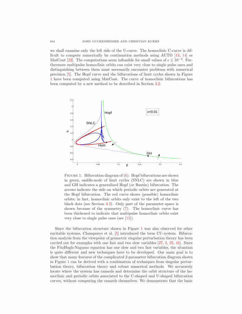
we shall examine only the left side of the U-curve. The homoclinic C-curve is dif-ficult to compute numerically by continuation methods using AUTO [13, 14] orMatCont [22]. The computations seem infeasible for small values of ǫ ≤ 10−3. Fur-thermore multipulse homoclinic orbits can exist very close to single pulse ones anddistinguishing between them must necessarily encounter problems with numericalprecision [5]. The Hopf curve and the bifurcations of limit cycles shown in Figure1 have been computed using MatCont. The curve of homoclinic bifurcations hasbeen computed by a new method to be described in Section 3.2.

0 0.05 0.1 0.15 0.2 0.25

0.4

0.6

0.8

1

1.2

1.4

1.6

1.8

2

2.2

p

s

GH

Hopf

Hom

SNLC

ε=0.01

Figure 1. Bifurcation diagram of (6). Hopf bifurcations are shownin green, saddle-node of limit cycles (SNLC) are shown in blueand GH indicates a generalized Hopf (or Bautin) bifurcation. Thearrows indicate the side on which periodic orbits are generated atthe Hopf bifurcation. The red curve shows (possible) homoclinicorbits; in fact, homoclinic orbits only exist to the left of the twoblack dots (see Section 3.2). Only part of the parameter space isshown because of the symmetry (7). The homoclinic curve hasbeen thickened to indicate that multipulse homoclinic orbits existvery close to single pulse ones (see [15]).

Since the bifurcation structure shown in Figure 1 was also observed for otherexcitable systems, Champneys et al. [5] introduced the term CU-system. Bifurca-tion analysis from the viewpoint of geometric singular perturbation theory has beencarried out for examples with one fast and two slow variables [27, 2, 25, 41]. Sincethe FitzHugh-Nagumo equation has one slow and two fast variables, the situationis quite different and new techniques have to be developed. Our main goal is toshow that many features of the complicated 2-parameter bifurcation diagram shownin Figure 1 can be derived with a combination of techniques from singular pertur-bation theory, bifurcation theory and robust numerical methods. We accuratelylocate where the system has canards and determine the orbit structure of the ho-moclinic and periodic orbits associated to the C-shaped and U-shaped bifurcationcurves, without computing the canards themselves. We demonstrate that the basic


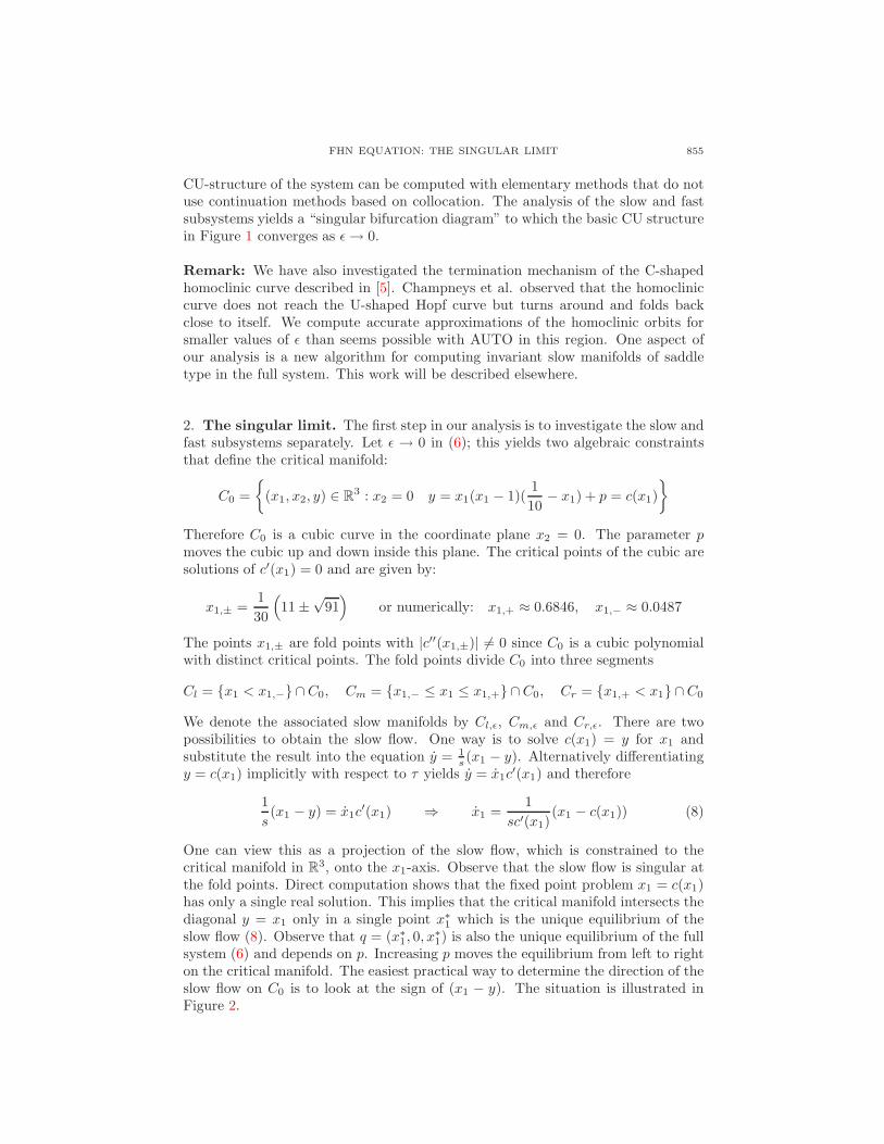
CU-structure of the system can be computed with elementary methods that do notuse continuation methods based on collocation. The analysis of the slow and fastsubsystems yields a “singular bifurcation diagram” to which the basic CU structurein Figure 1 converges as ǫ → 0.

Remark: We have also investigated the termination mechanism of the C-shapedhomoclinic curve described in [5]. Champneys et al. observed that the homocliniccurve does not reach the U-shaped Hopf curve but turns around and folds backclose to itself. We compute accurate approximations of the homoclinic orbits forsmaller values of ǫ than seems possible with AUTO in this region. One aspect ofour analysis is a new algorithm for computing invariant slow manifolds of saddletype in the full system. This work will be described elsewhere.

2. The singular limit. The first step in our analysis is to investigate the slow andfast subsystems separately. Let ǫ → 0 in (6); this yields two algebraic constraintsthat define the critical manifold:

C0 =

{

(x1, x2, y) ∈ R3 : x2 = 0 y = x1(x1 − 1)(

1

10− x1) + p = c(x1)

}

Therefore C0 is a cubic curve in the coordinate plane x2 = 0. The parameter pmoves the cubic up and down inside this plane. The critical points of the cubic aresolutions of c′(x1) = 0 and are given by:

x1,± =1

30

(

11 ±√

91)

or numerically: x1,+ ≈ 0.6846, x1,− ≈ 0.0487

The points x1,± are fold points with |c′′(x1,±)| 6= 0 since C0 is a cubic polynomialwith distinct critical points. The fold points divide C0 into three segments

Cl = {x1 < x1,−} ∩C0, Cm = {x1,− ≤ x1 ≤ x1,+} ∩C0, Cr = {x1,+ < x1} ∩C0

We denote the associated slow manifolds by Cl,ǫ, Cm,ǫ and Cr,ǫ. There are twopossibilities to obtain the slow flow. One way is to solve c(x1) = y for x1 andsubstitute the result into the equation y = 1

s (x1 − y). Alternatively differentiatingy = c(x1) implicitly with respect to τ yields y = x1c

′(x1) and therefore

1

s(x1 − y) = x1c

′(x1) ⇒ x1 =1

sc′(x1)(x1 − c(x1)) (8)

One can view this as a projection of the slow flow, which is constrained to thecritical manifold in R

3, onto the x1-axis. Observe that the slow flow is singular atthe fold points. Direct computation shows that the fixed point problem x1 = c(x1)has only a single real solution. This implies that the critical manifold intersects thediagonal y = x1 only in a single point x∗

1 which is the unique equilibrium of theslow flow (8). Observe that q = (x∗

1, 0, x∗1) is also the unique equilibrium of the full

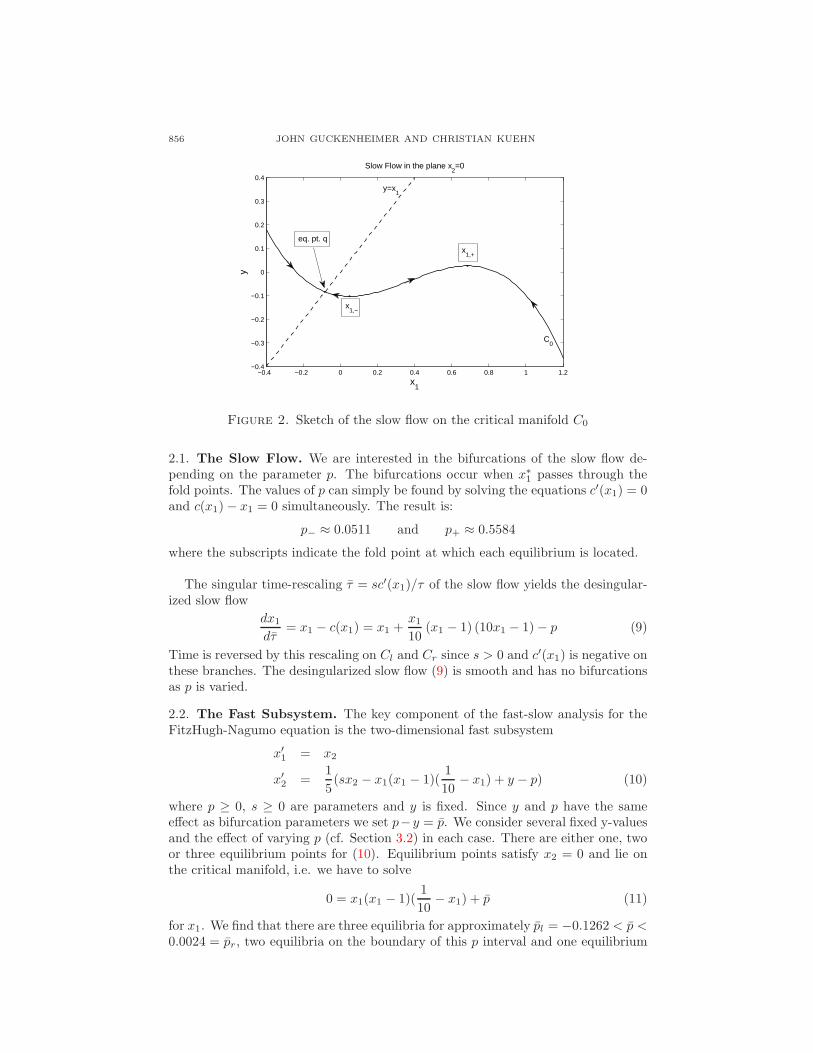
system (6) and depends on p. Increasing p moves the equilibrium from left to righton the critical manifold. The easiest practical way to determine the direction of theslow flow on C0 is to look at the sign of (x1 − y). The situation is illustrated inFigure 2.


−0.4 −0.2 0 0.2 0.4 0.6 0.8 1 1.2−0.4

−0.3

−0.2

−0.1

0

0.1

0.2

0.3

0.4

x1

y

Slow Flow in the plane x2=0

C0

eq. pt. q

y=x1

x1,+

x1,−

Figure 2. Sketch of the slow flow on the critical manifold C0

2.1. The Slow Flow. We are interested in the bifurcations of the slow flow de-pending on the parameter p. The bifurcations occur when x∗

1 passes through thefold points. The values of p can simply be found by solving the equations c′(x1) = 0and c(x1) − x1 = 0 simultaneously. The result is:

p− ≈ 0.0511 and p+ ≈ 0.5584

where the subscripts indicate the fold point at which each equilibrium is located.

The singular time-rescaling τ = sc′(x1)/τ of the slow flow yields the desingular-ized slow flow

dx1

dτ= x1 − c(x1) = x1 +

x1

10(x1 − 1) (10x1 − 1) − p (9)

Time is reversed by this rescaling on Cl and Cr since s > 0 and c′(x1) is negative onthese branches. The desingularized slow flow (9) is smooth and has no bifurcationsas p is varied.

2.2. The Fast Subsystem. The key component of the fast-slow analysis for theFitzHugh-Nagumo equation is the two-dimensional fast subsystem

x′1 = x2

x′2 =

1

5(sx2 − x1(x1 − 1)(

1

10− x1) + y − p) (10)

where p ≥ 0, s ≥ 0 are parameters and y is fixed. Since y and p have the sameeffect as bifurcation parameters we set p−y = p. We consider several fixed y-valuesand the effect of varying p (cf. Section 3.2) in each case. There are either one, twoor three equilibrium points for (10). Equilibrium points satisfy x2 = 0 and lie onthe critical manifold, i.e. we have to solve

0 = x1(x1 − 1)(1

10− x1) + p (11)

for x1. We find that there are three equilibria for approximately pl = −0.1262 < p <0.0024 = pr, two equilibria on the boundary of this p interval and one equilibrium


otherwise. The Jacobian of (10) at an equilibrium is

A(x1) =

(

0 1150

(

1 − 22x1 + 30x21

)

s5

)

Direct calculation yields that for p 6∈ [pl, pr] the single equilibrium is a saddle. Inthe case of three equilibria, we have a source that lies between two saddles. Notethat this also describes the stability of the three branches of the critical mani-fold Cl, Cm and Cr. For s > 0 the matrix A is singular of rank 1 if and only if30x2

1−22x1+1 = 0 which occurs for the fold points x1,±. Hence the equilibria of thefast subsystem undergo a fold (or saddle-node) bifurcation once they approach thefold points of the critical manifold. This happens for parameter values pl and pr.Note that by symmetry we can reduce to studying a single fold point. In the limits = 0 (corresponding to the case of a “standing wave”) the saddle-node bifurcationpoint becomes more degenerate with A(x1) nilpotent.

Our next goal is to investigate global bifurcations of (10); we start with homo-clinic orbits. For s = 0 it is easy to see that (10) is a Hamiltonian system:

x′1 =

∂H

∂x2= x2

x′2 = − ∂H

∂x1=

1

5(−x1(x1 − 1)(

1

10− x1) − p) (12)

with Hamiltonian function

H(x1, x2) =1

2x2

2 −(x1)

2

100+

11(x1)3

150− (x1)

4

20+

x1p

5(13)

We will use this Hamiltonian formulation later on to describe the geometry of ho-moclinic orbits for slow wave speeds. Assume that p is chosen so that (12) has ahomoclinic orbit x0(t). We are interested in perturbations with s > 0 and note thatin this case the divergence of (10) is s. Hence the vector field is area expandingeverywhere. The homoclinic orbit breaks for s > 0 and no periodic orbits are cre-ated. Note that this scenario does not apply to the full three-dimensional systemas the equilibrium q has a pair of complex conjugate eigenvalues so that a Shilnikovscenario can occur. This illustrates that the singular limit can be used to help locatehomoclinic orbits of the full system, but that some characteristics of these orbitschange in the singular limit.

We are interested next in finding curves in (p, s)-parameter space that representheteroclinic connections of the fast subsystem. The main motivation is the decom-position of trajectories in the full system into slow and fast segments. Concatenatingfast heteroclinic segments and slow flow segments can yield homoclinic orbits of thefull system [28, 4, 32, 38]. We describe a numerical strategy to detect heteroclinicconnections in the fast subsystem and continue them in parameter space. Supposethat p ∈ (pl, pr) so that (10) has three hyperbolic equilibrium points xl, xm andxr. We denote by Wu(xl) the unstable and by W s(xl) the stable manifold of xl.The same notation is also used for xr and tangent spaces to W s(.) and Wu(.) aredenoted by T s(.) and T u(.). Recall that xm is a source and shall not be of interestto us for now. Define the cross section Σ by

Σ = {(x1, x2) ∈ R2 : x1 =

xl + xr

2}.


We use forward integration of initial conditions in T u(xl) and backward integrationof initial conditions in T s(xr) to obtain trajectories γ+ and γ− respectively. Wecalculate their intersection with Σ and define

γl(p, s) := γ+ ∩ Σ, γr(p, s) := γ− ∩ Σ

We compute the functions γl and γr for different parameter values of (p, s) numer-ically. Heteroclinic connections occur at zeros of the function

h(p, s) := γl(p, s) − γr(p, s)

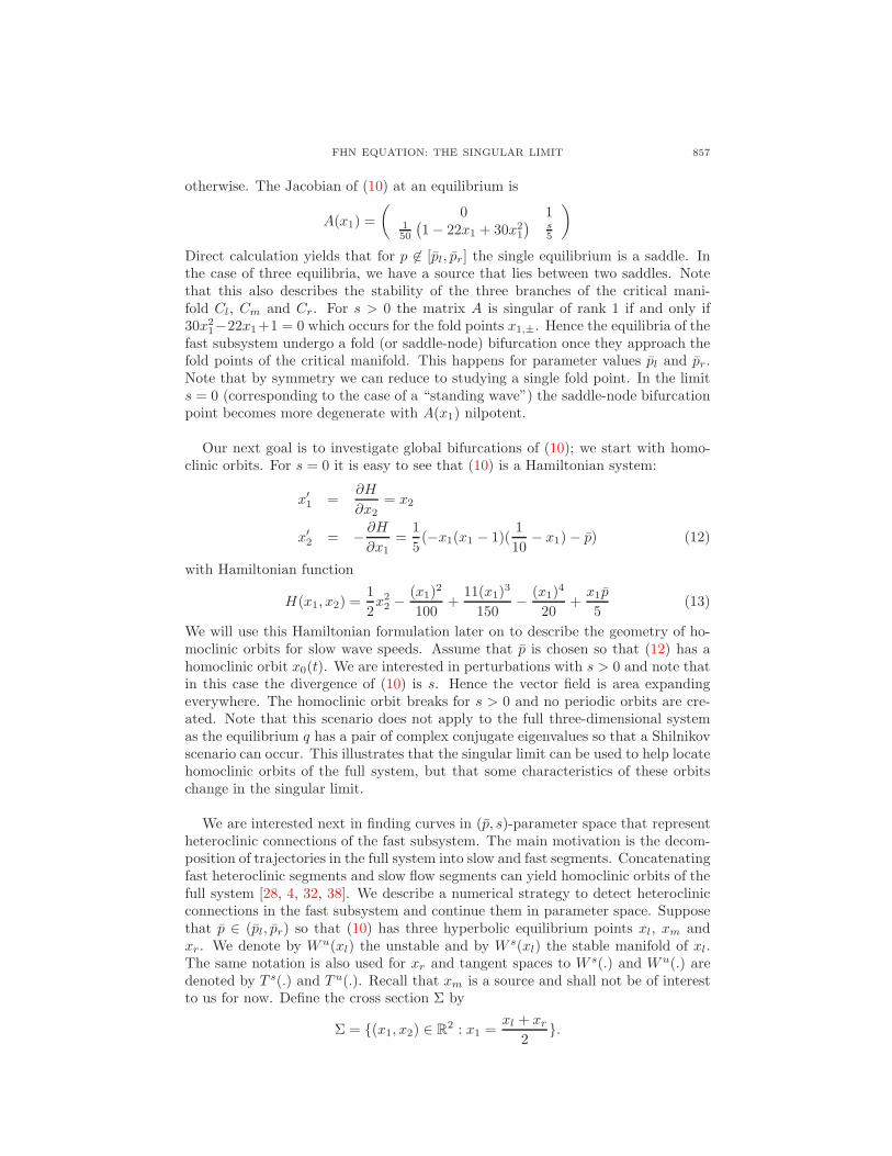
Once we find a parameter pair (p0, s0) such that h(p0, s0) = 0, these parameters canbe continued along a curve of heteroclinic connections in (p, s) parameter space bysolving the root-finding problem h(p0 + δ1, s0 + δ2) = 0 for either δ1 or δ2 fixed andsmall. We use this method later for different fixed values of y to compute heteroclinicconnections in the fast subsystem in (p, s) parameter space. The results of thesecomputations are illustrated in Figure 3. There are two distinct branches in Figure3. The branches are asymptotic to pl and pr and approximately form a “V ”. FromFigure 3 we conjecture that there exists a double heteroclinic orbit for p ≈ −0.0622.

−0.15 −0.1 −0.05 0 0.050

0.5

1

1.5

p

s

Figure 3. Heteroclinic connections for equation (10) in parameter space.

Remarks : If we fix p = 0 our initial change of variable becomes −y = p and ourresults for heteroclinic connections are for the FitzHugh-Nagumo equation withoutan applied current. In this situation it has been shown that the heteroclinic connec-tions of the fast subsystem can be used to prove the existence of homoclinic orbitsto the unique saddle equilibrium (0, 0, 0) (cf. [32]). Note that the existence of theheteroclinics in the fast subsystem was proved in a special case analytically [1] butFigure 3 is - to the best of our knowledge - the first explicit computation of wherefast subsystem heteroclinics are located. The paper [36] develops a method forfinding heteroclinic connections by the same basic approach we used, i.e. defininga codimension one hyperplane H that separates equilibrium points.

Figure 3 suggests that there exists a double heteroclinic connection for s = 0.

Observe that the Hamiltonian in our case is H(x1, x2) = (x2)2

2 + V (x1) where thefunction V (x1) is:

V (x1) =px1

5− (x1)

2

100+

11(x1)3

150− (x1)

4

20


The solution curves of (12) are given by x2 = ±√

2(const. − V (x1)). The structureof the solution curves entails symmetry under reflection about the x1-axis. Supposep ∈ [pl, pr] and recall that we denoted the two saddle points of (10) by xl and xr

and that their location depends on p. Therefore, we conclude that the two saddlesxl and xr must have a heteroclinic connection if they lie on the same energy level,i.e. they satisfy V (xl) − V (xr) = 0. This equation can be solved numerically tovery high accuracy.

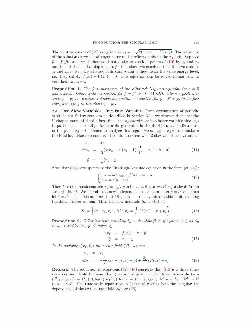
Proposition 1. The fast subsystem of the FitzHugh-Nagumo equation for s = 0has a double heteroclinic connection for p = p∗ ≈ −0.0619259. Given a particularvalue y = y0 there exists a double heteroclinic connection for p = p∗ + y0 in the fastsubsystem lying in the plane y = y0.

2.3. Two Slow Variables, One Fast Variable. From continuation of periodicorbits in the full system - to be described in Section 3.1 - we observe that near theU-shaped curve of Hopf bifurcations the x2-coordinate is a faster variable than x1.In particular, the small periodic orbits generated in the Hopf bifurcation lie almostin the plane x2 = 0. Hence to analyze this region we set x2 = x2/ǫ to transformthe FitzHugh-Nagumo equation (6) into a system with 2 slow and 1 fast variable:

x1 = x2

ǫ2 ˙x2 =1

5(sǫx2 − x1(x1 − 1)(

1

10− x1) + y − p) (14)

y =1

s(x1 − y)

Note that (14) corresponds to the FitzHugh-Nagumo equation in the form (cf. (4)):{

uτ = 5ǫ2uxx + f(u) − w + pwτ = ǫ(u − w)

(15)

Therefore the transformation x2 = x2/ǫ can be viewed as a rescaling of the diffusionstrength by ǫ2. We introduce a new independent small parameter δ = ǫ2 and thenlet δ = ǫ2 → 0. This assumes that O(ǫ) terms do not vanish in this limit, yieldingthe diffusion free system. Then the slow manifold S0 of (14) is:

S0 =

{

(x1, x2, y) ∈ R3 : x2 =

1

sǫ(f(x1) − y + p)

}

(16)

Proposition 2. Following time rescaling by s, the slow flow of system (14) on S0

in the variables (x1, y) is given by

ǫx1 = f(x1) − y + p

y = x1 − y (17)

In the variables (x1, x2) the vector field (17) becomes

x1 = x2

ǫ ˙x2 = − 1

s2(x1 − f(x1) − p) +

x2

s(f ′(x1) − ǫ) (18)

Remark: The reduction to equations (17)-(18) suggests that (14) is a three time-scale system. Note however that (14) is not given in the three time-scale form(ǫ2z1, ǫz2, z3) = (h1(z), h2(z), h3(z)) for z = (z1, z2, z3) ∈ R

3 and hi : R3 → R

(i = 1, 2, 3). The time-scale separation in (17)-(18) results from the singular 1/ǫdependence of the critical manifold S0; see (16).


Proof. (of Proposition 2) Use the defining equation for the slow manifold (16) andsubstitute it into x1 = x2. A rescaling of time by t → st under the assumption thats > 0 yields the result (17). To derive (18) differentiate the defining equation of S0

with respect to time:

˙x2 =1

sǫ(x1f

′(x1) − y) =1

sǫ(x2f

′(x1) − y)

The equations y = 1s (x1−y) and y = −sǫx2+f(x1)+p yield the equations (18).

Before we start with the analysis of (17) we note that bifurcation calculationsfor (17) exist. For example, Rocsoreanu et al. [44] give a detailed overview on theFitzHugh equation (17) and collect many relevant references. Therefore we shallonly state the relevant bifurcation results and focus on the fast-slow structure andcanards. Equation (17) has a critical manifold given by y = f(x1) + p = c(x1)which coincides with the critical manifold of the full FitzHugh-Nagumo system (6).Formally it is located in R

2 but we still denote it by C0. Recall that the fold pointsare located at

x1,± =1

30

(

11 ±√

91)

or numerically: x1,+ ≈ 0.6846, x1,− ≈ 0.0487

Also recall that the y-nullcline passes through the fold points at:

p− ≈ 0.0511 and p+ ≈ 0.5584

We easily find that supercritical Hopf bifurcations are located at the values

pH,±(ǫ) =2057

6750±√

11728171

182250000− 359ǫ

1350+

509ǫ2

2700− ǫ3

27(19)

For the case ǫ = 0.01 we get pH,−(0.01) ≈ 0.05632 and pH,+(0.01) ≈ 0.55316.The periodic orbits generated in the Hopf bifurcations exist for p ∈ (pH,−, pH,+).Observe also that pH,±(0) = p±; so the Hopf bifurcations of (17) coincide in thesingular limit with the fold bifurcations in the one-dimensional slow flow (8). Weare also interested in canards in the system and calculate a first order asymptoticexpansion for the location of the maximal canard in (17) following [37]; recall thattrajectories lying in the intersection of attracting and repelling slow manifolds arecalled maximal canards. We restrict to canards near the fold point (x1,−, c(x1,−)).

Proposition 3. Near the fold point (x1,−, c(x1,−)) the maximal canard in (p, ǫ)parameter space is given by:

p(ǫ) = x1,− − c(x1,−) +5

8ǫ + O(ǫ3/2)

Proof. Let y = y − p and consider the shifts

x1 → x1 + x1,−, y → y + c(x1,−), p → p + x1,− − c(x1,−)

to translate the equilibrium of (17) to the origin when p = 0. This gives

x′1 = x2

1

(√91

10− x1

)

− y = f(x1, y)

y′ = ǫ(x1 − y − p) = ǫ(g(x1, y) − p) (20)

Now apply Theorem 3.1 in [37] to find that the maximal canard of (20) is given by:

p(ǫ) =5

8ǫ + O(ǫ3/2)

Shifting the parameter p back to the original coordinates yields the result.


If we substitute ǫ = 0.01 in the previous asymptotic result and neglect terms oforder O(ǫ3/2) then the maximal canard is predicted to occur for p ≈ 0.05731 which isright after the first supercritical Hopf bifurcation at pH,− ≈ 0.05632. Therefore weexpect that there exist canard orbits evolving along the middle branch of the criticalmanifold Cm,0.01 in the full FitzHugh-Nagumo equation. Maximal canards are partof a process generally referred to as canard explosion [10, 39, 7]. In this situationthe small periodic orbits generated in the Hopf bifurcation at p = pH,− undergo atransition to relaxation oscillations within a very small interval in parameter space.A variational integral determines whether the canards are stable [39, 26].

Proposition 4. The canard cycles generated near the maximal canard point inparameter space for equation (17) are stable.

Proof. Consider the differential equation (17) in its transformed form (20). Obvi-ously this will not affect the stability analysis of any limit cycles. Let xl(h) andxm(h) denote the two smallest x1-coordinates of the intersection between

C0 := {(x1, y) ∈ R2 : y =

√91

10x2

1 − x31 = φ(x1)}

and the line y = h. Geometrically xl represents a point on the left branch and xm

a point on the middle branch of the critical manifold C0. Theorem 3.4 in [39] tellsus that the canards are stable cycles if the function

R(h) =

∫ xm(h)

xl(h)

∂f

∂x1(x1, φ(x1))

φ′(x1)

g(x1, φ(x1))dx1

is negative for all values h ∈ (0, φ(√

9115 )] where x1 =

√91

15 is the second fold point of

C0 besides x1 = 0. In our case we have

R(h) =

∫ xm(h)

xl(h)

(√

915 x1 − 3x2

1)2

x −√

9110 x2

1 + x31

dx

with xl(h) ∈ [−√

9130 , 0) and xm(h) ∈ (0,

√91

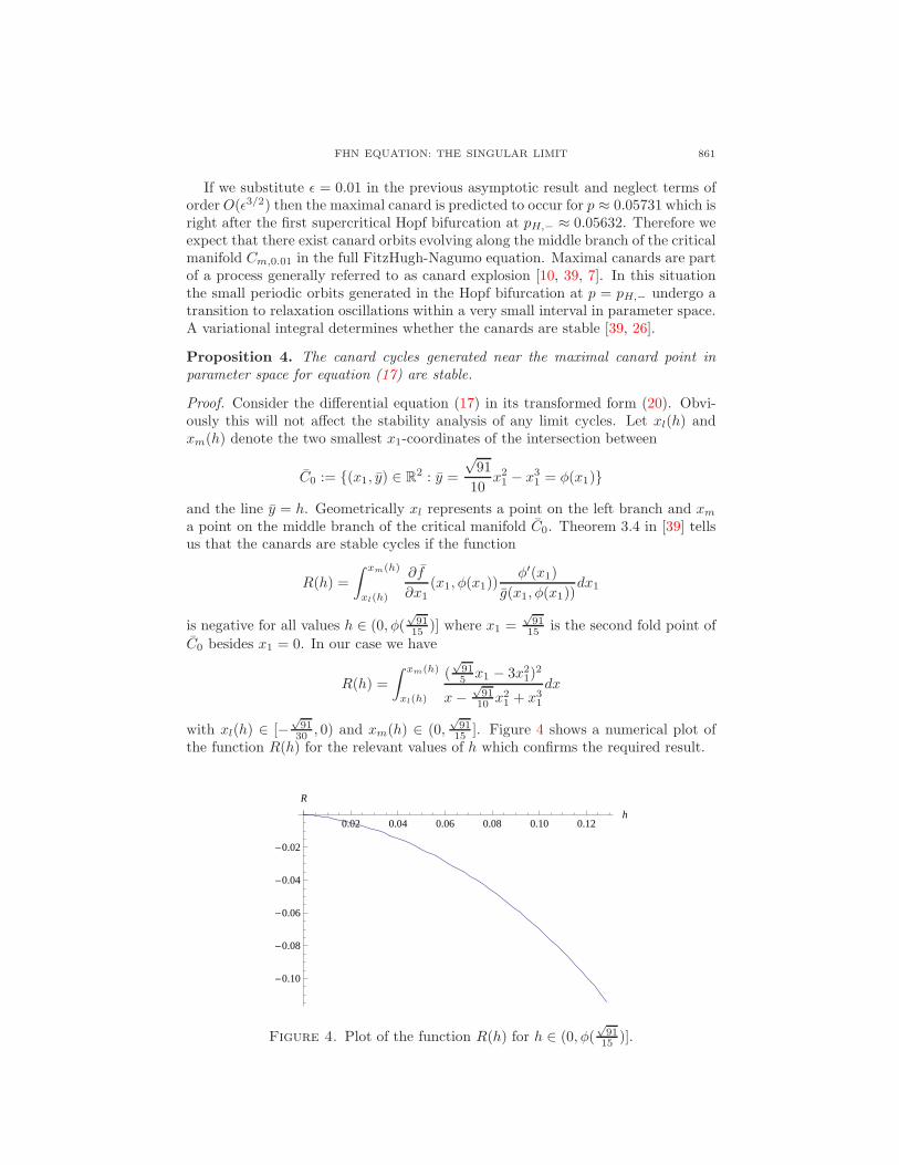
15 ]. Figure 4 shows a numerical plot ofthe function R(h) for the relevant values of h which confirms the required result.

0.02 0.04 0.06 0.08 0.10 0.12h

-0.10

-0.08

-0.06

-0.04

-0.02

R

Figure 4. Plot of the function R(h) for h ∈ (0, φ(√

9115 )].


Remark: We have computed an explicit algebraic expression for R′(h) with a

computer algebra system. This expression yields R′(h) < 0 for h ∈ (0, φ(√

9115 )],

confirming that R(h) is decreasing.

As long as we stay on the critical manifold C0 of the full system, the analysis ofthe bifurcations and geometry of (17) give good approximations to the dynamicsof the FitzHugh-Nagumo equation because the rescaling x2 = ǫx2 leaves the planex2 = 0 invariant. Next we use the dynamics of the x2-coordinate in system (18) toobtain better insight into the dynamics when x2 6= 0. The critical manifold D0 of(18) is:

D0 = {(x1, x2) ∈ R2 : sx2c

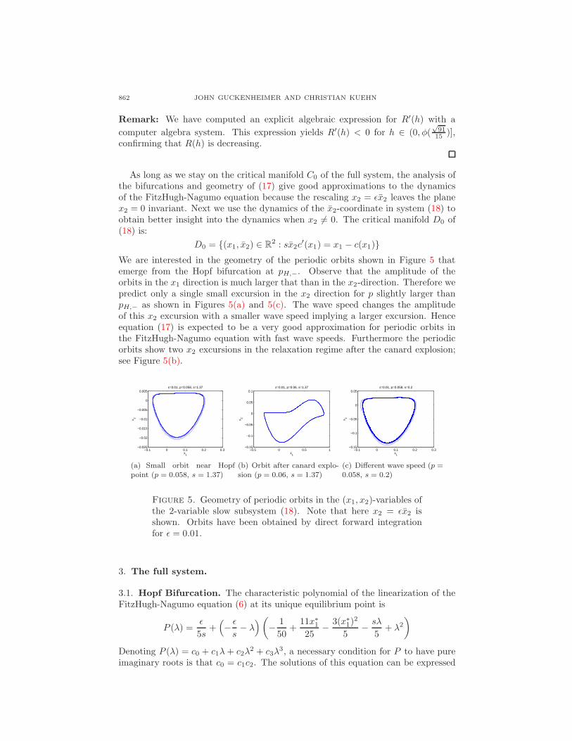
′(x1) = x1 − c(x1)}We are interested in the geometry of the periodic orbits shown in Figure 5 thatemerge from the Hopf bifurcation at pH,−. Observe that the amplitude of theorbits in the x1 direction is much larger that than in the x2-direction. Therefore wepredict only a single small excursion in the x2 direction for p slightly larger thanpH,− as shown in Figures 5(a) and 5(c). The wave speed changes the amplitudeof this x2 excursion with a smaller wave speed implying a larger excursion. Henceequation (17) is expected to be a very good approximation for periodic orbits inthe FitzHugh-Nagumo equation with fast wave speeds. Furthermore the periodicorbits show two x2 excursions in the relaxation regime after the canard explosion;see Figure 5(b).

−0.1 0 0.1 0.2 0.3−0.025

−0.02

−0.015

−0.01

−0.005

0

0.005

x1

x 2

ε=0.01, p=0.058, s=1.37

(a) Small orbit near Hopfpoint (p = 0.058, s = 1.37)

−0.5 0 0.5 1−0.15

−0.1

−0.05

0

0.05

0.1

x1

x 2

ε=0.01, p=0.06, s=1.37

(b) Orbit after canard explo-sion (p = 0.06, s = 1.37)

−0.1 0 0.1 0.2 0.3−0.15

−0.1

−0.05

0

0.05

x1

x 2

ε=0.01, p=0.058, s=0.2

(c) Different wave speed (p =0.058, s = 0.2)

Figure 5. Geometry of periodic orbits in the (x1, x2)-variables ofthe 2-variable slow subsystem (18). Note that here x2 = ǫx2 isshown. Orbits have been obtained by direct forward integrationfor ǫ = 0.01.

3. The full system.

3.1. Hopf Bifurcation. The characteristic polynomial of the linearization of theFitzHugh-Nagumo equation (6) at its unique equilibrium point is

P (λ) =ǫ

5s+(

− ǫ

s− λ)

(

− 1

50+

11x∗1

25− 3(x∗

1)2

5− sλ

5+ λ2

)

Denoting P (λ) = c0 + c1λ + c2λ2 + c3λ

3, a necessary condition for P to have pureimaginary roots is that c0 = c1c2. The solutions of this equation can be expressed


parametrically as a curve (p(x∗1), s(x

∗1)):

s(x∗1)

2 =50ǫ(ǫ − 1)

1 + 10ǫ − 22x∗1 + 30(x∗

1)2

p(x∗1) = (x∗

1)3 − 1.1(x∗

1)2 + 1.1 (21)

Proposition 5. In the singular limit ǫ → 0 the U-shaped bifurcation curves ofthe FitzHugh-Nagumo equation have vertical asymptotes given by the points p− ≈0.0510636 and p+ ≈ 0.558418 and a horizontal asymptote given by {(p, s) : p ∈[p−, p+] and s = 0}. Note that at p± the equilibrium point passes through thetwo fold points.

Proof. The expression for s(x∗1)

2 in (21) is positive when 1+10ǫ−22x∗1+30(x∗

1)2 < 0.

For values of x∗1 between the roots of 1− 22x∗

1 + 30(x∗1)

2 = 0, s(x∗1)

2 → 0 in (21) asǫ → 0. The values of p− and p+ in the proposition are approximations to the valueof p(x∗

1) in (21) at the roots of 1 − 22x∗1 + 30(x∗

1)2 = 0. As ǫ → 0, solutions of the

equation s(x∗1)

2 = c > 0 in (21) yield values of x∗1 that tend to one of the two roots

of 1 − 22x∗1 + 30(x∗

1)2 = 0. The result follows.

−0.1 −0.05 0 0.05 0.1 0.15 0.2 0.25 0.30.05

0.06

0.07

0.08

0.09

0.1

0.11

0.12

0.13

x1

y

p=0.0598C

0

p=0.0801

(a) Projection onto (x1, y)

−0.1 −0.05 0 0.05 0.1 0.15 0.2 0.25 0.3−0.025

−0.02

−0.015

−0.01

−0.005

0

0.005

0.01

0.015

x1

x 2

p=0.0598

p=0.0801

C0

(b) Projection onto (x1, x2)

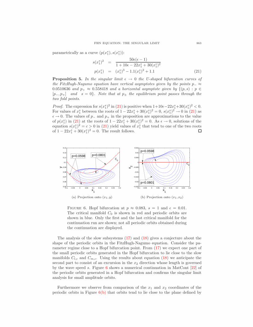
Figure 6. Hopf bifurcation at p ≈ 0.083, s = 1 and ǫ = 0.01.The critical manifold C0 is shown in red and periodic orbits areshown in blue. Only the first and the last critical manifold for thecontinuation run are shown; not all periodic orbits obtained duringthe continuation are displayed.

The analysis of the slow subsystems (17) and (18) gives a conjecture about theshape of the periodic orbits in the FitzHugh-Nagumo equation. Consider the pa-rameter regime close to a Hopf bifurcation point. From (17) we expect one part ofthe small periodic orbits generated in the Hopf bifurcation to lie close to the slowmanifolds Cl,ǫ and Cm,ǫ. Using the results about equation (18) we anticipate thesecond part to consist of an excursion in the x2 direction whose length is governedby the wave speed s. Figure 6 shows a numerical continuation in MatCont [22] ofthe periodic orbits generated in a Hopf bifurcation and confirms the singular limitanalysis for small amplitude orbits.

Furthermore we observe from comparison of the x1 and x2 coordinates of theperiodic orbits in Figure 6(b) that orbits tend to lie close to the plane defined by


x2 = 0. More precisely, the x2 diameter of the periodic orbits is observed to beO(ǫ) in this case. This indicates that the rescaling of Section 2.3 can help to de-scribe the system close to the U-shaped Hopf curve. Note that it is difficult tocheck whether this observation of an O(ǫ)-diameter in the x2-coordinate persistsfor values of ǫ < 0.01 since numerical continuation of canard-type periodic orbits isdifficult to use for smaller ǫ.

0.1706 0.1707 0.1708 0.1709 0.171 0.1711 0.17120

0.1

0.2

0.3

0.4

0.5

0.6

0.7

ε=0.01

ε=10−7

p

s

(a) GHǫ

1

0.051 0.052 0.053 0.054 0.055 0.056 0.057 0.058 0.0593.75

3.8

3.85

3.9

3.95

4

p

ε=0.01

s

ε=10−7

(b) GHǫ

2

Figure 7. Tracking of two generalized Hopf points (GH) in(p, s, ǫ)-parameter space. Each point in the figure corresponds toa different value of ǫ. The point GHǫ

1 in 7(a) corresponds to thepoint shown as a square in Figure 1 and the point GHǫ

2 in 7(b) isfurther up on the left branch of the U-curve and is not displayedin Figure 1.

In contrast to this, it is easily possible to compute the U-shaped Hopf curve us-ing numerical continuation for very small values of ǫ. We have used this possibilityto track two generalized Hopf bifurcation points in three parameters (p, s, ǫ). TheU-shaped Hopf curve has been computed by numerical continuation for a mesh ofparameter values for ǫ between 10−2 and 10−7 using MatCont [22]. The two general-ized Hopf points GHǫ

1,2 on the left half of the U-curve were detected as codimensiontwo points during each continuation run. The results of this “three-parameter con-tinuation” are shown in Figure 7.

The two generalized Hopf points depend on ǫ and we find that their singularlimits in (p, s)-parameter space are approximately:

GH01 ≈ (p = 0.171, s = 0) and GH0

2 ≈ (p = 0.051, s = 3.927)

We have not found a way to recover these special points from the fast-slow de-composition of the system. This suggests that codimension two bifurcations aregenerally diffcult to recover from the singular limit of fast-slow systems.

Furthermore the Hopf bifurcations for the full system on the left half of the U-curve are subcritical between GHǫ

1 and GHǫ2 and supercritical otherwise. For the

transformed system (14) with two slow and one fast variable we observed that inthe singular limit (17) for ǫ2 → 0 the Hopf bifurcation is supercritical. In the caseof ǫ = 0.01 the periodic orbits for (6) and (17) exist in overlapping regions for theparameter p between the p-values of GH0.01

1 and GH0.012 . This result indicates that


(14) can be used to describe periodic orbits that will interact with the homoclinicC-curve.

3.2. Homoclinic Orbits. In the following discussion we refer to “the” C-shapedcurve of homoclinic bifurcations of system (5) as the parameters yielding a “single-pulse” homoclinic orbit. The literature as described in Section 1.2 shows that closeto single-pulse homoclinic orbits we can expect multipulse homoclinic orbits thatreturn close to the equilibrium point multiple times. Since the separation of slowmanifolds C·,ǫ is exponentially small, homoclinic orbits of different types will alwaysoccur in exponentially thin bundles in parameter space. Values of ǫ < 0.005 aresmall enough that the parameter region containing all the homoclinic orbits will beindistinguishable numerically from “the” C-curve that we locate.

The history of proofs of the existence of homoclinic orbits in the FitzHugh-Nagumo equation is quite extensive. The main step in their construction is theexistence of a “singular” homoclinic orbit γ0. We consider the case when the fastsubsystem has three equilibrium points which we denote by xl ∈ Cl, xm ∈ Cm andxr ∈ Cr. Recall that xl coincides with the unique equilibrium q = (x∗

1, 0, x∗1) of the

full system for p < p−. A singular homoclinic orbit is always constructed by firstfollowing the unstable manifold of xl in the fast subsystem given by y = x∗

1.

0 0.5 1−0.2

−0.1

0

0.1

0.2

x1

x 2

p=−0.24602

0 0.5 1−0.2

−0.1

0

0.1

0.2

x1

x 2

p=−0.1

0 0.5 1−0.2

−0.1

0

0.1

0.2

x1

x 2

p=0

0 0.5 1−0.2

−0.1

0

0.1

0.2

x1

x 2

p=0.05

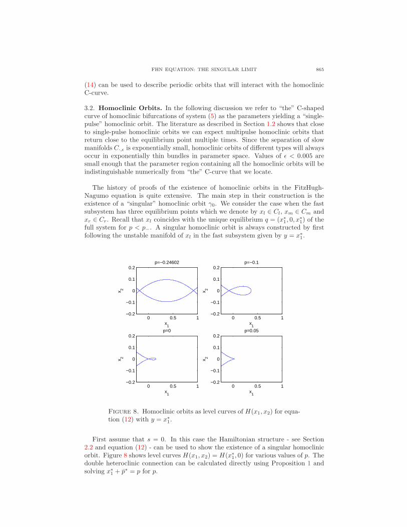
Figure 8. Homoclinic orbits as level curves of H(x1, x2) for equa-tion (12) with y = x∗

1.

First assume that s = 0. In this case the Hamiltonian structure - see Section2.2 and equation (12) - can be used to show the existence of a singular homoclinicorbit. Figure 8 shows level curves H(x1, x2) = H(x∗

1, 0) for various values of p. Thedouble heteroclinic connection can be calculated directly using Proposition 1 andsolving x∗

1 + p∗ = p for p.


Proposition 6. There exists a singular double heteroclinic connection in theFitzHugh-Nagumo equation for s = 0 and p ≈ −0.246016 = p∗.

Techniques developed in [45] show that the singular homoclinic orbits existingfor s = 0 and p ∈ (p∗, p−) must persist for perturbations of small positive wavespeed and sufficiently small ǫ. These orbits are associated to the lower branch ofthe C-curve. The expected geometry of the orbits is indicated by their shape inthe singular limit shown in Figure 8. The double heteroclinic connection is theboundary case between the upper and lower half of the C-curve. It remains toanalyze the singular limit for the upper half. In this case, a singular homoclinicorbit is again formed by following the unstable manifold of xl when it coincides withthe equilibrium q = (x∗

1, 0, x∗1) but now we check whether it forms a heteroclinic

orbit with the stable manifold of xr. Then we follow the slow flow on Cr and returnon a heteroclinic connection to Cl for a different y-coordinate with y > x∗

1 andy < c(x1,+) = f(x1) + p. From there we connect back via the slow flow. Usingthe numerical method described in Section 2.2 we first set y = x∗

1; note that thelocation of q depends on the value of the parameter p. The task is to check whenthe system

x′1 = x2

x′2 =

1

5(f(x1) + y − p) (22)

has heteroclinic orbits from Cl to Cr with y = x∗1. The result of this computation

is shown in Figure 9 as the red curve. We have truncated the result at p = −0.01.In fact, the curve in Figure 9 can be extended to p = p∗. Obviously we should viewthis curve as an approximation to the upper part of the C-curve.

−0.02 0 0.02 0.04 0.06 0.080.8

0.9

1

1.1

1.2

1.3

1.4

1.5

1.6

p

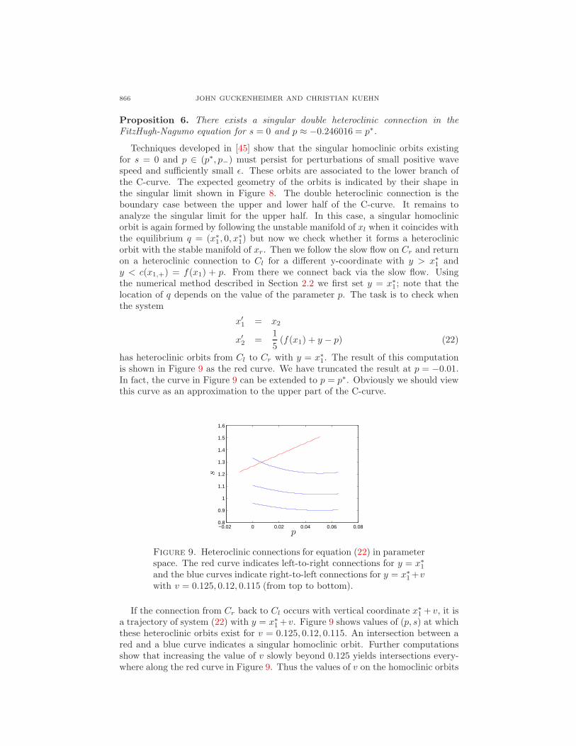
s

Figure 9. Heteroclinic connections for equation (22) in parameterspace. The red curve indicates left-to-right connections for y = x∗

1

and the blue curves indicate right-to-left connections for y = x∗1 +v

with v = 0.125, 0.12, 0.115 (from top to bottom).

If the connection from Cr back to Cl occurs with vertical coordinate x∗1 + v, it is

a trajectory of system (22) with y = x∗1 +v. Figure 9 shows values of (p, s) at which

these heteroclinic orbits exist for v = 0.125, 0.12, 0.115. An intersection between ared and a blue curve indicates a singular homoclinic orbit. Further computationsshow that increasing the value of v slowly beyond 0.125 yields intersections every-where along the red curve in Figure 9. Thus the values of v on the homoclinic orbits


are expected to grow as s increases along the upper branch of the C-curve. Sincethere cannot be any singular homoclinic orbits for p ∈ (p−, p+) we have to find theintersection of the red curve in Figure 9 with the vertical line p = p−. Using thenumerical method to detect heteroclinic connections gives:

Proposition 7. The singular homoclinic curve for positive wave speed terminatesat p = p− and s ≈ 1.50815 = s∗ on the right and at p = p∗ and s = 0 on the left.

In (p, s)-parameter space define the points:

A = (p∗, 0), B = (p−, 0), C = (p−, s∗) (23)

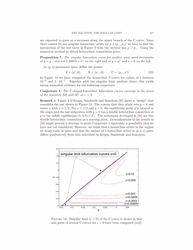
In Figure 10 we have computed the homoclinic C-curve for values of ǫ between10−2 and 5 · 10−5. Together with the singular limit analysis above, this yieldsstrong numerical evidence for the following conjecture:

Conjecture 1. The C-shaped homoclinic bifurcation curves converge to the unionof the segments AB and AC as ǫ → 0.

Remark 1: Figure 4 of Krupa, Sandstede and Szmolyan [38] shows a “wedge” thatresembles the one shown in Figure 10. The system that they study sets p = 0 andvaries a with a ≈ 1/2. For a = 1/2 and p = 0, the equilibrium point q is located atthe origin and the fast subsystem with y = 0 has a double heteroclinic connection atq to the saddle equilibrium (1, 0, 0) ∈ Cr. The techniques developed in [38] use thisdouble heteroclinic connection as a starting point. Generalizations of the results in[38] might provide a strategy to prove Conjecture 1 rigorously, a possibility that wehave not yet considered. However, we think that 1-homoclinic orbits in the regimewe study come in pairs and that the surface of 1-homoclinic orbits in (p, s, ǫ) spacediffers qualitatively from that described by Krupa, Sandstede and Szmolyan.

−0.25 −0.2 −0.15 −0.1 −0.05 0 0.050

0.2

0.4

0.6

0.8

1

1.2

1.4

1.6

p

s

ε=0.01

ε=0.005

ε=0.001ε=0.0005ε=0.0001

ε=0.00005

singular limit bifurcation curves ε=0

Figure 10. Singular limit (ǫ = 0) of the C-curve is shown in blueand parts of several C-curves for ǫ > 0 have been computed (red).


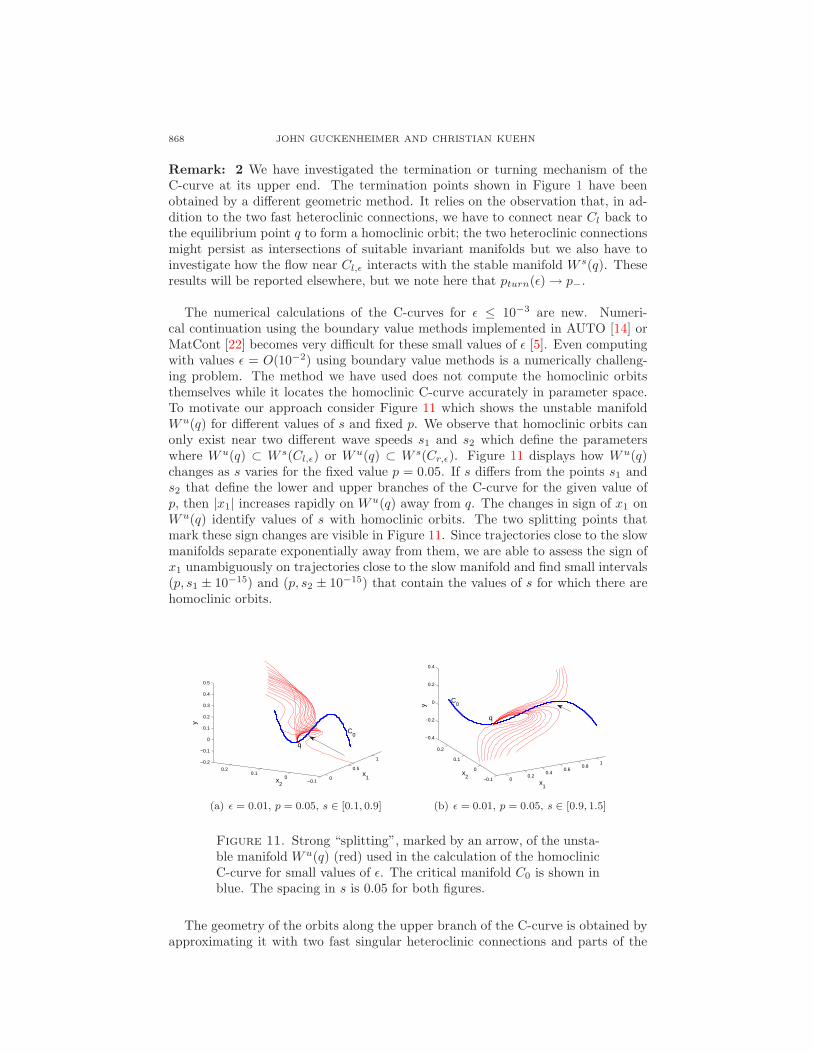
Remark: 2 We have investigated the termination or turning mechanism of theC-curve at its upper end. The termination points shown in Figure 1 have beenobtained by a different geometric method. It relies on the observation that, in ad-dition to the two fast heteroclinic connections, we have to connect near Cl back tothe equilibrium point q to form a homoclinic orbit; the two heteroclinic connectionsmight persist as intersections of suitable invariant manifolds but we also have toinvestigate how the flow near Cl,ǫ interacts with the stable manifold W s(q). Theseresults will be reported elsewhere, but we note here that pturn(ǫ) → p−.

The numerical calculations of the C-curves for ǫ ≤ 10−3 are new. Numeri-cal continuation using the boundary value methods implemented in AUTO [14] orMatCont [22] becomes very difficult for these small values of ǫ [5]. Even computingwith values ǫ = O(10−2) using boundary value methods is a numerically challeng-ing problem. The method we have used does not compute the homoclinic orbitsthemselves while it locates the homoclinic C-curve accurately in parameter space.To motivate our approach consider Figure 11 which shows the unstable manifoldWu(q) for different values of s and fixed p. We observe that homoclinic orbits canonly exist near two different wave speeds s1 and s2 which define the parameterswhere Wu(q) ⊂ W s(Cl,ǫ) or Wu(q) ⊂ W s(Cr,ǫ). Figure 11 displays how Wu(q)changes as s varies for the fixed value p = 0.05. If s differs from the points s1 ands2 that define the lower and upper branches of the C-curve for the given value ofp, then |x1| increases rapidly on Wu(q) away from q. The changes in sign of x1 onWu(q) identify values of s with homoclinic orbits. The two splitting points thatmark these sign changes are visible in Figure 11. Since trajectories close to the slowmanifolds separate exponentially away from them, we are able to assess the sign ofx1 unambiguously on trajectories close to the slow manifold and find small intervals(p, s1 ± 10−15) and (p, s2 ± 10−15) that contain the values of s for which there arehomoclinic orbits.

0

0.5

1

−0.10

0.10.2

−0.2

−0.1

0

0.1

0.2

0.3

0.4

0.5

x1x

2

y

C0

q

(a) ǫ = 0.01, p = 0.05, s ∈ [0.1, 0.9]

00.2

0.40.6

0.81

−0.1

0

0.1

0.2

−0.4

−0.2

0

0.2

0.4

x1

x2

y

C0

q

(b) ǫ = 0.01, p = 0.05, s ∈ [0.9, 1.5]

Figure 11. Strong “splitting”, marked by an arrow, of the unsta-ble manifold Wu(q) (red) used in the calculation of the homoclinicC-curve for small values of ǫ. The critical manifold C0 is shown inblue. The spacing in s is 0.05 for both figures.

The geometry of the orbits along the upper branch of the C-curve is obtained byapproximating it with two fast singular heteroclinic connections and parts of the


slow manifolds Cr,ǫ and Cl,ǫ; this process has been described several times in theliterature when different methods were used to prove the existence of “fast waves”(see e.g. [29, 4, 32]).

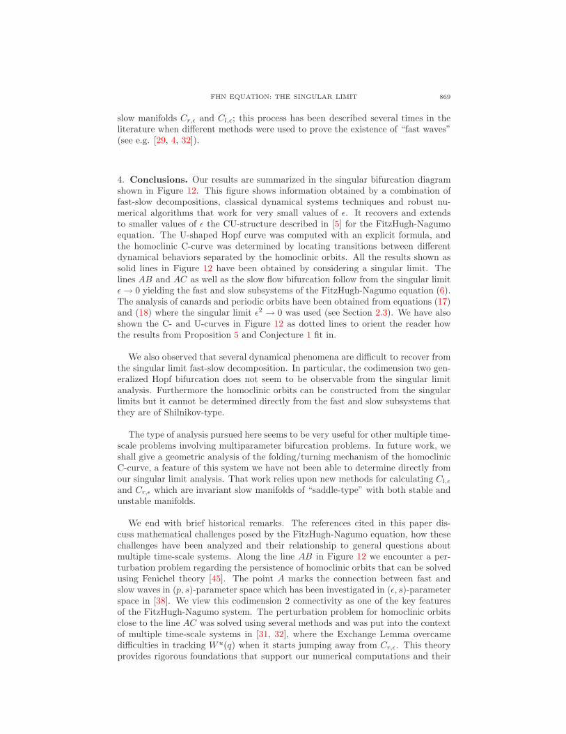
4. Conclusions. Our results are summarized in the singular bifurcation diagramshown in Figure 12. This figure shows information obtained by a combination offast-slow decompositions, classical dynamical systems techniques and robust nu-merical algorithms that work for very small values of ǫ. It recovers and extendsto smaller values of ǫ the CU-structure described in [5] for the FitzHugh-Nagumoequation. The U-shaped Hopf curve was computed with an explicit formula, andthe homoclinic C-curve was determined by locating transitions between differentdynamical behaviors separated by the homoclinic orbits. All the results shown assolid lines in Figure 12 have been obtained by considering a singular limit. Thelines AB and AC as well as the slow flow bifurcation follow from the singular limitǫ → 0 yielding the fast and slow subsystems of the FitzHugh-Nagumo equation (6).The analysis of canards and periodic orbits have been obtained from equations (17)and (18) where the singular limit ǫ2 → 0 was used (see Section 2.3). We have alsoshown the C- and U-curves in Figure 12 as dotted lines to orient the reader howthe results from Proposition 5 and Conjecture 1 fit in.

We also observed that several dynamical phenomena are difficult to recover fromthe singular limit fast-slow decomposition. In particular, the codimension two gen-eralized Hopf bifurcation does not seem to be observable from the singular limitanalysis. Furthermore the homoclinic orbits can be constructed from the singularlimits but it cannot be determined directly from the fast and slow subsystems thatthey are of Shilnikov-type.

The type of analysis pursued here seems to be very useful for other multiple time-scale problems involving multiparameter bifurcation problems. In future work, weshall give a geometric analysis of the folding/turning mechanism of the homoclinicC-curve, a feature of this system we have not been able to determine directly fromour singular limit analysis. That work relies upon new methods for calculating Cl,ǫ

and Cr,ǫ which are invariant slow manifolds of “saddle-type” with both stable andunstable manifolds.

We end with brief historical remarks. The references cited in this paper dis-cuss mathematical challenges posed by the FitzHugh-Nagumo equation, how thesechallenges have been analyzed and their relationship to general questions aboutmultiple time-scale systems. Along the line AB in Figure 12 we encounter a per-turbation problem regarding the persistence of homoclinic orbits that can be solvedusing Fenichel theory [45]. The point A marks the connection between fast andslow waves in (p, s)-parameter space which has been investigated in (ǫ, s)-parameterspace in [38]. We view this codimension 2 connectivity as one of the key featuresof the FitzHugh-Nagumo system. The perturbation problem for homoclinic orbitsclose to the line AC was solved using several methods and was put into the contextof multiple time-scale systems in [31, 32], where the Exchange Lemma overcamedifficulties in tracking Wu(q) when it starts jumping away from Cr,ǫ. This theoryprovides rigorous foundations that support our numerical computations and their

870

JO

HN

GU

CK

EN

HE

IME

RA

ND

CH

RIS

TIA

NK

UE

HN

het

het

het/hom

hom

periodic

periodic

periodic

hom

x1

x1

x1

x1

x1x1

x1

x1

x2

x2

x2x2

y

y

y

y

p

s

AB

C

Canards in equation (17),(18)

C-curve

U-curve

slow flow bifurcation p = p−

Hopf bif. pH,− in (17),(18)

Figure 12. Sketch of the singular bifurcation diagram for the FitzHugh-Nagumo equation (6). The points A, B and Care defined in (23). The part of the diagram obtained from equations (17),(18) corresponds to the case “ǫ2 = 0 and ǫ 6= 0and small”. In this scenario the canards to the right of p = p− are stable (see Proposition 4). The phase portrait inthe upper right for equation (17) shows the geometry of a small periodic orbit generated in the Hopf bifurcation of (17).The two phase portraits below it show the geometry of these periodic orbits further away from the Hopf bifurcation for(17),(18). Excursions of the periodic orbits/canards for p > p− decrease for larger values of s. Note also that we haveindicated as dotted lines the C-curve and the U-curve for positive ǫ to allow a qualitative comparison with Figure 1.


interpretation.

Acknowledgments. This research was partially supported by the National ScienceFoundation and Department of Energy.

REFERENCES

[1] D. G. Aronson and H. F. Weinberger, Nonlinear diffusion in population genetics, combustion,and nerve pulse propagation, in “Partial Differential Equations and Related Topics” (LectureNotes in Mathematics), 446 (1974), 5–49.

[2] K. Bold, C. Edwards, J. Guckenheimer, S. Guharay, K. Hoffman, Judith Hubbard, RicardoOliva, and Waren Weckesser, The forced van der Pol equation 2: Canards in the reducedsystem, SIAM Journal of Applied Dynamical Systems, 2 (2003), 570–608.

[3] P. Brunovsky, Tracking invariant manifolds without differential forms, Acta Math. Univ.Comenianae, LXV (1996), 23–32.

[4] Gail A. Carpenter, A geometric approach to singular perturbation problems with applicationsto nerve impulse equations, Journal of Differential Equations, 23 (1977), 335–367.

[5] A. R. Champneys, V. Kirk, E. Knobloch, B. E. Oldeman and J. Sneyd, When Shil’nikov meetshopf in excitable systems, SIAM Journal of Applied Dynamical Systems, 6 (2007), 663–693.

[6] Bo Deng, The existence of infinitely many traveling front and back waves in the FitzHugh-Nagumo equations, SIAM J. Appl. Math., 22 (1991), 1631–1650.

[7] M. Diener, The canard unchained or how fast/slow dynamical systems bifurcate, The Math-ematical Intelligencer, 6 (1984), 38–48.

[8] Francine Diener and Marc Diener, “Nonstandard Analysis in Practice,” Springer, 1995.[9] Freddy Dumortier, Techniques in the theory of local bifurcations: Blow-up, normal forms,

nilpotent bifurcations, singular perturbations, in: Bifurcations and Periodic Orbits of VectorFields [D. Schlomiuk (ed.)], 19–73, 1993.

[10] Freddy Dumortier and R. Roussarie, Canard cycles and center manifolds, Memoirs of theAmerican Mathematical Society, 121 (1996).

[11] Wiktor Eckhaus, Relaxation oscillations including a standard chase on french ducks, LectureNotes in Mathematics, 985 (1983), 449–494.

[12] V. I. Arnold (Ed.), “Encyclopedia of Mathematical Sciences: Dynamical Systems V.,”Springer, 1994.

[13] E. J. Doedel et al, Auto 97: Continuation and bifurcation software for ordinary differentialequations, http://indy.cs.concordia.ca/auto , 1997.

[14] E. J. Doedel et al, Auto 2000: Continuation and bifurcation software for ordinary differentialequations (with homcont), http://cmvl.cs.concordia.ca/auto , 2000.

[15] John W. Evans, Neil Fenichel and John A. Feroe, Double impulse solutions in nerve axonequations, SIAM J. Appl. Math., 42 (1982), 219–234.

[16] Neil Fenichel, Persistence and smoothness of invariant manifolds for flows, Indiana UniversityMathematical Journal, 21 (1971), 193–225.

[17] Neil Fenichel, Asymptotic stability with rate conditions, Indiana University MathematicalJournal, 23 (1974), 1109–1137.

[18] Neil Fenichel, Asymptotic stability with rate conditions II, Indiana University MathematicalJournal, 26 (1977), 81–93.

[19] Neil Fenichel, Geometric singular perturbation theory for ordinary differential equations,Journal of Differential Equations, 31 (1979), 53–98.

[20] R. FitzHugh, Mathematical models of threshold phenomena in the nerve membrane, Bull.Math. Biophysics, 17 (1955), 257–269.

[21] Gilberto Flores, Stability analysis for the slow traveling pulse of the FitzHugh-Nagumo system,SIAM J. Math. Anal., 22 (1991), 392–399.

[22] W. Govaerts and Yu. A. Kuznetsov, “Matcont,” http://www.matcont.ugent.be/ , 2008.[23] Johan Grasman, “Asymptotic Methods for Relaxation Oscillations and Applications,”

Springer, 1987.[24] John Guckenheimer, Bifurcation and degenerate decomposition in multiple time scale dynam-

ical systems, in “Nonlinear Dynamics and Chaos: Where do We Go from Here?” Eds.: JohnHogan, Alan Champneys and Bernd Krauskopf, 1–20, 2002.

http://www.ams.org/mathscinet-getitem?mr=MR0427837&return=pdf










http://indy.cs.concordia.ca/auto

http://cmvl.cs.concordia.ca/auto







http://www.matcont.ugent.be/




[25] John Guckenheimer, Global bifurcations of periodic orbits in the forced van der Pol equation,in “Global Analysis of Dynamical Systems - Festschrift dedicated to Floris Takens,” Eds.:Henk W. Broer, Bernd Krauskopf and Gert Vegter, 1–16, 2003.

[26] John Guckenheimer, Bifurcations of relaxation oscillations, Normal forms, bifurcations andfiniteness problems in differential equations, NATO Sci. Ser. II Math. Phys. Chem., 137

(2004), 295–316.[27] John Guckenheimer, Kathleen Hoffman and Warren Weckesser, The forced van der Pol equa-

tion 1: The slow flow and its bifurcations, SIAM Journal of Applied Dynamical Systems, 2

(2003), 1–35.[28] S. P. Hastings, Some mathematical problems from neurobiology, The American Mathematical

Monthly, 82 (1975), 881–895.[29] S. P. Hastings, On the existence of homoclinic and periodic orbits in the FitzHugh-Nagumo

equations, Quart. J. Math. Oxford, 2 (1976), 123–134.[30] A. L. Hodgin and A. F. Huxley, A quantitative description of membrane current and its

application to conduction and excitation in nerve, J. Physiol., 117 (1952), 500–505.[31] C. Jones and N. Kopell, Tracking invariant manifolds with differential forms in singularly

perturbed systems, Journal of Differential Equations, 108 (1994), 64–88.[32] C. Jones, N. Kopell and R. Langer, Construction of the FitzHugh-Nagumo pulse using dif-

ferential forms, Patterns and dynamics in reactive media (Minneapolis, MN, 1989), 101–115,IMA Vol. Math. Appl., 37, Springer, New York, 1991.

[33] Christopher K. R. T. Jones, Stability of the travelling wave solution of the FitzHugh-Nagumosystem, Transactions of the American Mathematical Society, 286 (1984), 431–469.

[34] Christopher K. R. T. Jones, “Geometric Singular Perturbation Theory: In Dynamical Sys-tems” (Montecatini Terme, 1994). Springer, 1995.

[35] Christopher K. R. T. Jones, Tasso J. Kaper and Nancy Kopell, Tracking invariant manifoldsup tp exponentially small errors, SIAM Journal of Mathematical Analysis, 27 (1996), 558–577.

[36] B. Krauskopf and T. Riess, A Lin’s method approach to finding and continuing heteroclinicconnections involving periodic orbits, Nonlinearity, 21 (2008), 1655–1690.

[37] M. Krupa and P. Szmolyan, Extending geometric singular perturbation theory to nonhyper-bolic points - fold and canard points in two dimensions, SIAM J. Math. Anal., 33 (2001),

286–314.[38] Martin Krupa, Bjoern Sandstede and Peter Szmolyan, Fast and slow waves in the FitzHugh-

Nagumo equation, Journal of Differential Equations, 133 (1997), 49–97.[39] Martin Krupa and Peter Szmolyan, Relaxation oscillation and canard explosion, Journal of

Differential Equations, 174 (2001), 312–368.[40] X-B Lin, Using Melnikov’s method to solve Shilnikov’s problems, Proc. Roy. Soc. Edinburgh,

116 (1990), 295–325.[41] Alexandra Milik and Peter Szmolyan, Multiple time scales and canards in a chemical oscilla-

tor, in “Multiple-Time-Scale Dynamical Systems,” Eds.: Christopher K. R. T. Jones (Editor)and Alexander I. Khibnik (Editor), 2001.

[42] E. F. Mishchenko and N. Kh. Rozov, “Differential Equations with Small Parameters andRelaxation Oscillations” (translated from Russian), Plenum Press, 1980.

[43] J. Nagumo, S. Arimoto and S. Yoshizawa, An active pulse transmission line simulating nerveaxon, Proc. IRE, 50 (1962), 2061–2070.

[44] C. Rocsoreanu, A. Georgescu and N. Giurgiteanu, “The FitzHugh-Nagumo Model - Bifurca-tion and Dynamics,” Kluwer, 2000.

[45] Peter Szmolyan, Transversal heteroclinic and homoclinic orbits in singular perturbation prob-lems, Journal of Differential Equations, 92 (1991), 252–281.

[46] Peter Szmolyan and Martin Wechselberger, Canards in R3, Journal of Differential Equations,

177 (2001), 419–453.

Received September 2008; revised April 2009.

E-mail address: [email protected]

E-mail address: [email protected]




















homoclinic orbits of the fitzhugh-nagumo equation: the ...math.cornell.edu/~gucken/pdf/fhnc.pdf ·...

Documents