hidden markov models, iii. algorithms -...

Hidden MarkovModels, III.Algorithms

Steven R.Dunbar

Review ofAlgorithms

Baum-WelchAlgorithm

Overall PathProblem

Scaling andPracticalConsiderations

Example

Hidden Markov Models, III. Algorithms

Steven R. Dunbar

March 3, 2017

1 / 23


Steven R.Dunbar

Review ofAlgorithms

Baum-WelchAlgorithm

Overall PathProblem


Example

Outline

1 Review of Algorithms

2 Baum-Welch Algorithm

3 Overall Path Problem

4 Scaling and Practical Considerations

5 Example

2 / 23


Steven R.Dunbar

Review ofAlgorithms

Baum-WelchAlgorithm

Overall PathProblem


Example

Forward Algorithm

The forward algorithm or alpha pass. Fort = 0, 1, 2, . . . T − 1 and i = 0, 1, . . . , N − 1, define

αt(i) = P [O0,O1,O2, . . .Ot, xt = qi |λ]

Then αt(i) is the probability of the partial observation ofthe sequence up to time t with the Markov process instate qi at time t.

3 / 23


Steven R.Dunbar

Review ofAlgorithms

Baum-WelchAlgorithm

Overall PathProblem


Example

Recursive computation

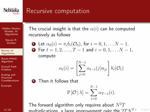
The crucial insight is that the α(i) can be computedrecursively as follows

1 Let α0(i) = πibi(O0), for i = 0, 1, . . . N − 1.2 For t = 1, 2, . . . , T − 1 and i = 0, 1, . . . N − 1,

compute

αt(i) =

[N−1∑j=0

αt−1(j)aji

]bi(Ot)

3 Then it follows that

P [O |λ] =N−1∑i=0

αT−1(i).

The forward algorithm only requires about N2Tmultiplications, a large improvement over the 2TNT

multiplications for the naive approach.

4 / 23


Steven R.Dunbar

Review ofAlgorithms

Baum-WelchAlgorithm

Overall PathProblem


Example

Backward Algorithm

The backward algorithm, or beta-pass. This isanalogous to the alpha-pass described in the solution tothe first problem of HMMs, except that it starts at theend and works back toward the beginning.

It is independent of the forward algorithm, so it can bedone in parallel.

5 / 23


Steven R.Dunbar

Review ofAlgorithms

Baum-WelchAlgorithm

Overall PathProblem


Example

Recursive computation

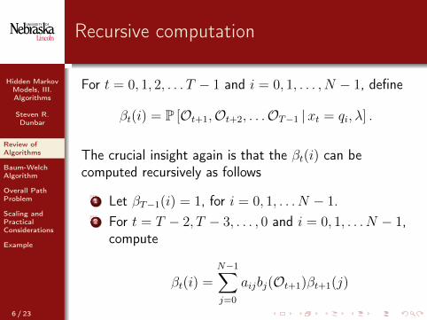
For t = 0, 1, 2, . . . T − 1 and i = 0, 1, . . . , N − 1, define

βt(i) = P [Ot+1,Ot+2, . . .OT−1 |xt = qi, λ] .

The crucial insight again is that the βt(i) can becomputed recursively as follows

1 Let βT−1(i) = 1, for i = 0, 1, . . . N − 1.2 For t = T − 2, T − 3, . . . , 0 and i = 0, 1, . . . N − 1,

compute

βt(i) =N−1∑j=0

aijbj(Ot+1)βt+1(j)

6 / 23


Steven R.Dunbar

Review ofAlgorithms

Baum-WelchAlgorithm

Overall PathProblem


Example

The Viterbi (Forward-Backward) Algorithm

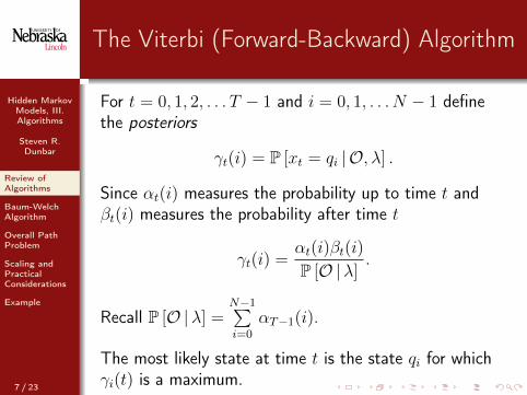
For t = 0, 1, 2, . . . T − 1 and i = 0, 1, . . . N − 1 definethe posteriors

γt(i) = P [xt = qi | O, λ] .

Since αt(i) measures the probability up to time t andβt(i) measures the probability after time t

γt(i) =αt(i)βt(i)

P [O |λ].

Recall P [O |λ] =N−1∑i=0

αT−1(i).

The most likely state at time t is the state qi for whichγi(t) is a maximum.7 / 23


Steven R.Dunbar

Review ofAlgorithms

Baum-WelchAlgorithm

Overall PathProblem


Example

Problem 3: Training and Parameter Fitting

Given an observation sequence O and the dimensions Nand M , find the model λ = (A,B, π) that maximizes theprobability of O. This can interpreted as training amodel to best fit the observed data. We can also viewthis as search in the parameter space represented by A,B and π.

The solution of Problem 3 attempts to optimize themodel parameters so as best to describe how theobserved sequence comes about. The observed sequenceused to solve Problem 3 is called a training sequencesince it is used to train the model. This training problemis the crucial one for most applications of hidden Markovmodels since it creates best models for real phenomena.

8 / 23


Steven R.Dunbar

Review ofAlgorithms

Baum-WelchAlgorithm

Overall PathProblem


Example

Baum-Welch Algorithm

For t = 0, 1, . . . , T − 2 and i, j ∈ {0, 1, . . . , N − 1},define

ξt(i, j) = P [xt = qi, xt+1 = qj | O, λ]

so ξt(i, j) is the probability of being in state qi at time tand transitioning to state qj at time t+ 1. They can bewritten in terms of α, β, A and B as

ξt(i, j) =αt(i)aijbj(Ot+1)βt+1(j)

P [O |λ]

For t = 0, 1, . . . , T − 2, γt(i) and ξt(i, j) are related by

γt(i) =N−1∑j=0

ξt(i, j)

9 / 23


Steven R.Dunbar

Review ofAlgorithms

Baum-WelchAlgorithm

Overall PathProblem


Example

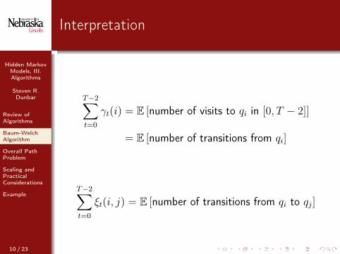
Interpretation

T−2∑t=0

γt(i) = E [number of visits to qi in [0, T − 2]]

= E [number of transitions from qi]

T−2∑t=0

ξt(i, j) = E [number of transitions from qi to qj]

10 / 23


Steven R.Dunbar

Review ofAlgorithms

Baum-WelchAlgorithm

Overall PathProblem


Example

Estimation

π = γ0(i) = expected freq. in qi at t = 0

aij =exptd. trans. from qi to qj

exptd. trans. from qi=

T−2∑t=0

ξ(i, j)

T−2∑t=0

γt(i)

bi(k) =exptd. times in qi emitting k

exptd. times in qi=

∑t∈{0,...,T−1}Ot=k

γt(i)

T−1∑t=0

γt(i)

11 / 23


Steven R.Dunbar

Review ofAlgorithms

Baum-WelchAlgorithm

Overall PathProblem


Example

Training and Estimating Parameters

Re-estimation is an iterative process. First we initializeλ = (A,B, π) with a best guess, or if no reasonableguess is available, we choose random values such thatπi ≈ 1/N and aij ≈ 1/N and bj(k) ≈ 1/M . It is criticalthat A, B and π be randomized since exactly uniformvalues results in a local maximum from which the modelcannot climb. As always, A, B, π must be rowstochastic.

12 / 23


Steven R.Dunbar

Review ofAlgorithms

Baum-WelchAlgorithm

Overall PathProblem


Example

Iterative Process

1 Initialize λ = (A,B, π) with a best guess.2 Compute αt(i), βt(i), γt(i), ξt(i, j).3 Re-estimate the modelλ = (A,B, π).4 If P [O |λ] increases by at least some predetermined

threshold or the predetermined maximum number ofiterations has not been exceeded, go to step 2.

5 Else stop and output λ = (A,B, π).

13 / 23


Steven R.Dunbar

Review ofAlgorithms

Baum-WelchAlgorithm

Overall PathProblem


Example

Overall Path Problem

Find the most likely overall path given the observations(not the states which are individually most likely).

Dynamic Programming algorithm is the forwardalgorithm with "sum" replaced by "max"

14 / 23


Steven R.Dunbar

Review ofAlgorithms

Baum-WelchAlgorithm

Overall PathProblem


Example

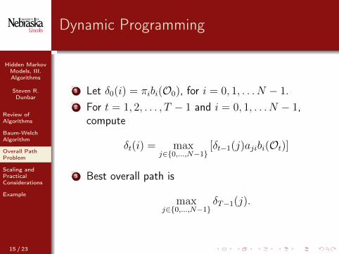
Dynamic Programming

1 Let δ0(i) = πibi(O0), for i = 0, 1, . . . N − 1.2 For t = 1, 2, . . . , T − 1 and i = 0, 1, . . . N − 1,

compute

δt(i) = maxj∈{0,...,N−1}

[δt−1(j)ajibi(Ot)]

3 Best overall path is

maxj∈{0,...,N−1}

δT−1(j).

15 / 23


Steven R.Dunbar

Review ofAlgorithms

Baum-WelchAlgorithm

Overall PathProblem


Example

Note about the path

The Dynamic Programming Algorithm only gives theoptimal probability, not the path.

Must keep track of preceding states at each stage, traceback from the highest-scoring final state.

16 / 23


Steven R.Dunbar

Review ofAlgorithms

Baum-WelchAlgorithm

Overall PathProblem


Example

Underflow problems

All computations involve multiple products ofprobabilities, hence tend to 0 quickly at T increases.Therefore, underflow is a serious problem.

Solution is to scale all computations.

17 / 23


Steven R.Dunbar

Review ofAlgorithms

Baum-WelchAlgorithm

Overall PathProblem


Example

Scaled Forward Algorithm

1 1 Let α0(i) = α0(i) for i = 0, 1, . . . , N − 1.

2 Let c0 = 1

/N−1∑j=0

α0(j)

3 Let α(i) = c0α0(i) for i = 0, 1, . . . , N − 1.2 For i = 0, 1, . . . , N − 1, compute

α(i) =N−1∑j=0

αt−1(j)ajibi(Ot)

3 Let ct = 1

/N−1∑j=0

α(j)

4 By induction αt(i) = c0c1 · · · ct Thenαt(i) = αt(i)

N−1∑j=0

αt(j)

18 / 23


Steven R.Dunbar

Review ofAlgorithms

Baum-WelchAlgorithm

Overall PathProblem


Example

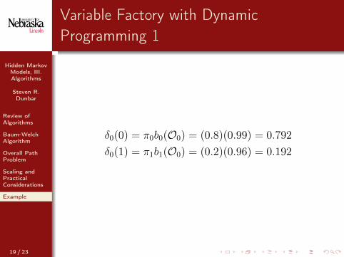
Variable Factory with DynamicProgramming 1

δ0(0) = π0b0(O0) = (0.8)(0.99) = 0.792

δ0(1) = π1b1(O0) = (0.2)(0.96) = 0.192

19 / 23


Steven R.Dunbar

Review ofAlgorithms

Baum-WelchAlgorithm

Overall PathProblem


Example

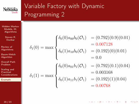
Variable Factory with DynamicProgramming 2

δ1(0) = max

δ0(0)a00b0(O1) = (0.792)(0.9)(0.01)

= 0.007128

δ0(1)a10b0(O1) = (0.192)(0)(0.01)

= 0.0

δ1(1) = max

δ0(0)a01b1(O1) = (0.792)(0.1)(0.04)

= 0.003168

δ0(1)a11b1(O1) = (0.192)(1)(0.04)

= 0.00768

20 / 23


Steven R.Dunbar

Review ofAlgorithms

Baum-WelchAlgorithm

Overall PathProblem


Example

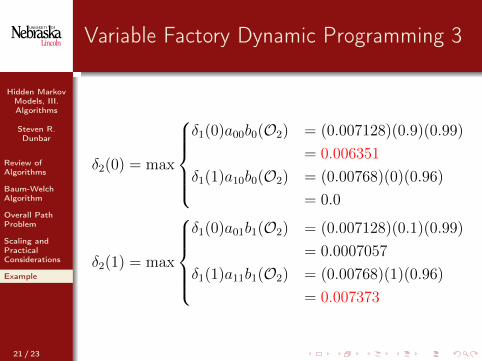
Variable Factory Dynamic Programming 3

δ2(0) = max

δ1(0)a00b0(O2) = (0.007128)(0.9)(0.99)

= 0.006351

δ1(1)a10b0(O2) = (0.00768)(0)(0.96)

= 0.0

δ2(1) = max

δ1(0)a01b1(O2) = (0.007128)(0.1)(0.99)

= 0.0007057

δ1(1)a11b1(O2) = (0.00768)(1)(0.96)

= 0.007373

21 / 23


Steven R.Dunbar

Review ofAlgorithms

Baum-WelchAlgorithm

Overall PathProblem


Example

Variable Factory Dynamic Programming 4

δt(i) 0 (a) 1 (u) 2 (a)0 0.792 0.007128 0.0063511 0.192 0.00768 0.007373

Tracing back the source of the red maximum, themaximum overall state sequence was 111, same asexhaustive search.

22 / 23


Steven R.Dunbar

Review ofAlgorithms

Baum-WelchAlgorithm

Overall PathProblem


Example

Remarks on Efficiency

The simple example required only 18 multiplicationscompared to 40 for the exhaustive listing of allpossibilities.

Not surprising, since DP throws out one path of two atevery stage.

Similar efficiency for larger problems

23 / 23

hidden markov models, iii. algorithms -...

Documents