hidden markov models and gaussian mixture models · hidden markov models and gaussian mixture...
TRANSCRIPT
Hidden Markov Modelsand
Gaussian Mixture Models
Hiroshi Shimodaira and Steve Renals
Automatic Speech Recognition— ASR Lectures 4&526&30 January 2017
ASR Lectures 4&5 Hidden Markov Models and Gaussian Mixture Models 1

Overview
HMMs and GMMs
Key models and algorithms for HMM acoustic models
Gaussians
GMMs: Gaussian mixture models
HMMs: Hidden Markov models
HMM algorithms
Likelihood computation (forward algorithm)Most probable state sequence (Viterbi algorithm)Estimting the parameters (EM algorithm)
ASR Lectures 4&5 Hidden Markov Models and Gaussian Mixture Models 2

Fundamental Equation of Statistical Speech Recognition
If X is the sequence of acoustic feature vectors (observations) andW denotes a word sequence, the most likely word sequence W∗ isgiven by
W∗ = arg maxW
P(W |X)
Applying Bayes’ Theorem:
P(W |X) =p(X |W)P(W)
p(X)
∝ p(X |W)P(W)
W∗ = arg maxW
p(X |W)︸ ︷︷ ︸Acoustic
model
P(W)︸ ︷︷ ︸Language
model
NB: X is used hereafter to denote the output feature vectors from the
signal analysis module rather than DFT spectrum.ASR Lectures 4&5 Hidden Markov Models and Gaussian Mixture Models 3

Acoustic Modelling
AcousticModel
Lexicon
LanguageModel
Recorded Speech
SearchSpace
Decoded Text (Transcription)
TrainingData
SignalAnalysis
Hidden Markov Model
ASR Lectures 4&5 Hidden Markov Models and Gaussian Mixture Models 4

Hierarchical modelling of speech
"No right"
NO RIGHT
ohn r ai t
Utterance
Word
Subword
HMM
Acoustics
Generative Model
ASR Lectures 4&5 Hidden Markov Models and Gaussian Mixture Models 5
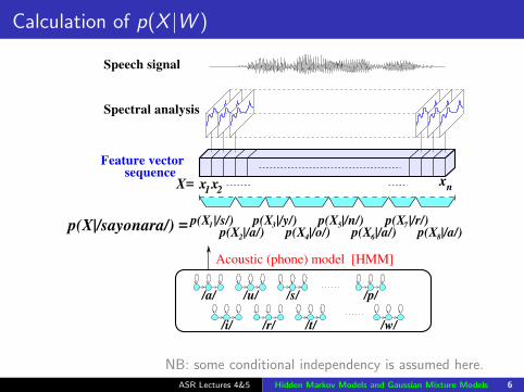
Calculation of p(X |W )
p(X |/a/)6 p(X |/a/)8
p(X |/s/)1
2p(X |/a/)
21
p(X |/o/)4
nx
p(X |/n/) p(X |/r/)75p(X |/y/)3
X= xx
p(X|/sayonara/) =
sequenceFeature vector
Speech signal
Spectral analysis
Acoustic (phone) model [HMM]
/s//u/ /p/
/i/
/a/
/t/ /w//r/
NB: some conditional independency is assumed here.
ASR Lectures 4&5 Hidden Markov Models and Gaussian Mixture Models 6

How to calculate p(X1|/s/)?
Assume x1, x2, · · · , xT1 corresponds to phoneme /s/,the conditional probability that we observe the sequence is
p(X1|/s/) = p(x1, · · · , xT1 |/s/), x i = (x1i , · · · , xdi )t ∈ Rd
We know that HMM can be employed to calculate this. (Viterbialgorithm, Forward / Backward algorithm)
To grasp the idea of probability calculation, let’s consider anextremely simple case where the length of input sequence is justone (T1 = 1), and the dimensionality of x is one (d = 1), so thatwe don’t need HMM.
p(X1|/s/) −→ p(x1|/s/)
ASR Lectures 4&5 Hidden Markov Models and Gaussian Mixture Models 7

How to calculate p(X1|/s/)? (cont.)
p(x |/s/) : conditional probability(conditional probability density function (pdf) of x)
A Gaussian / normal distribution function could be employedfor this:
P(x |/s/) =1√
2πσ2se− (x−µs )2
2σ2s
The function has only two parameters, µs and σ2s
Given a set of training samples {x, · · · , xN}, we canestimate µs and σs
µs = 1N
∑Ni=1xi, σ2s = 1
N
∑Ni=1(xi − µs)2
For a general case where a phone lasts more than one frame,we need to employ HMM.
ASR Lectures 4&5 Hidden Markov Models and Gaussian Mixture Models 8

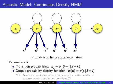
Acoustic Model: Continuous Density HMM
s1 s2 s3 sEP(s2 | s1)
P(s2 | s2)
p(x | s2)
x
p(x | s1)
x x
P(s1|sI)
p(x | s3)
sIP(s3 | s2) P(sE | s3)
P(s3 | s3)P(s1 | s1)
Probabilistic finite state automaton
Paramaters λ:
Transition probabilities: akj = P(S = j |S =k)Output probability density function: bj(x) = p(x |S = j)NB: Some textbooks use Q or q to denote the state variable S .
x corresponds to ot in Lecture slides 02.
ASR Lectures 4&5 Hidden Markov Models and Gaussian Mixture Models 9
Acoustic Model: Continuous Density HMM
s1 s2 s3 sEsI
x3x1 x2 x4 x5 x6
Probabilistic finite state automaton
Paramaters λ:
Transition probabilities: akj = P(S = j |S =k)Output probability density function: bj(x) = p(x |S = j)NB: Some textbooks use Q or q to denote the state variable S .
x corresponds to ot in Lecture slides 02.
ASR Lectures 4&5 Hidden Markov Models and Gaussian Mixture Models 9
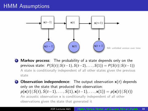
HMM Assumptions
s(t!1) s(t) s(t+1)
x(t + 1)x(t ! 1) x(t)NB: unfolded version over time
1 Markov process: The probability of a state depends only on theprevious state: P(S(t) |S(t−1),S(t−2), . . . , S(1)) = P(S(t) |S(t−1))A state is conditionally independent of all other states given the previous
state
2 Observation independence: The output observation x(t) dependsonly on the state that produced the observation:p(x(t) |S(t),S(t−1), . . . ,S(1), x(t−1), . . . , x(1)) = p(x(t) |S(t))An acoustic observation x is conditionally independent of all other
observations given the state that generated it
ASR Lectures 4&5 Hidden Markov Models and Gaussian Mixture Models 10
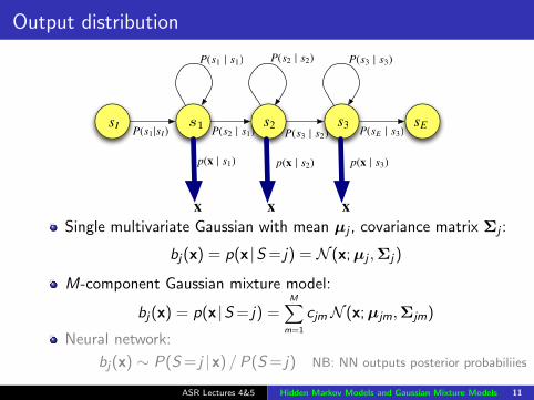
Output distribution
s1 s2 s3 sEP(s2 | s1)
P(s2 | s2)
p(x | s2)
x
p(x | s1)
x x
P(s1|sI)
p(x | s3)
sIP(s3 | s2) P(sE | s3)
P(s3 | s3)P(s1 | s1)
Single multivariate Gaussian with mean µj , covariance matrix Σj :
bj(x) = p(x |S = j) = N (x;µj ,Σj)
M-component Gaussian mixture model:
bj(x) = p(x |S = j) =M∑
m=1
cjmN (x;µjm,Σjm)
Neural network:
bj(x) ∼ P(S = j |x) /P(S = j) NB: NN outputs posterior probabiliies
ASR Lectures 4&5 Hidden Markov Models and Gaussian Mixture Models 11
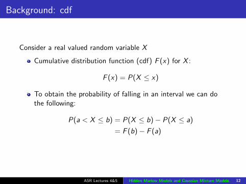
Background: cdf
Consider a real valued random variable X
Cumulative distribution function (cdf) F (x) for X :
F (x) = P(X ≤ x)
To obtain the probability of falling in an interval we can dothe following:
P(a < X ≤ b) = P(X ≤ b)− P(X ≤ a)
= F (b)− F (a)
ASR Lectures 4&5 Hidden Markov Models and Gaussian Mixture Models 12
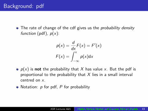
Background: pdf
The rate of change of the cdf gives us the probability densityfunction (pdf), p(x):
p(x) =d
dxF (x) = F ′(x)
F (x) =
∫ x
−∞p(x)dx
p(x) is not the probability that X has value x . But the pdf isproportional to the probability that X lies in a small intervalcentred on x .
Notation: p for pdf, P for probability
ASR Lectures 4&5 Hidden Markov Models and Gaussian Mixture Models 13

The Gaussian distribution (univariate)
The Gaussian (or Normal) distribution is the most common(and easily analysed) continuous distribution
It is also a reasonable model in many situations (the famous“bell curve”)
If a (scalar) variable has a Gaussian distribution, then it has aprobability density function with this form:
p(x |µ, σ2) = N (x ;µ, σ2) =1√
2πσ2exp
(−(x − µ)2
2σ2
)The Gaussian is described by two parameters:
the mean µ (location)the variance σ2 (dispersion)
ASR Lectures 4&5 Hidden Markov Models and Gaussian Mixture Models 14

Plot of Gaussian distribution
Gaussians have the same shape, with the location controlledby the mean, and the spread controlled by the variance
One-dimensional Gaussian with zero mean and unit variance(µ = 0, σ2 = 1):
−4 −3 −2 −1 0 1 2 3 40
0.05
0.1
0.15
0.2
0.25
0.3
0.35
0.4
x
p(x|
m,s
)
pdf of Gaussian Distribution
mean=0variance=1
ASR Lectures 4&5 Hidden Markov Models and Gaussian Mixture Models 15

Properties of the Gaussian distribution
N (x ;µ, σ2) =1√
2πσ2exp
(−(x − µ)2
2σ2
)
−8 −6 −4 −2 0 2 4 6 80
0.05
0.1
0.15
0.2
0.25
0.3
0.35
0.4
x
p(x|
m,s
)pdfs of Gaussian distributions
mean=0variance=1
mean=0variance=2
mean=0variance=4
ASR Lectures 4&5 Hidden Markov Models and Gaussian Mixture Models 16
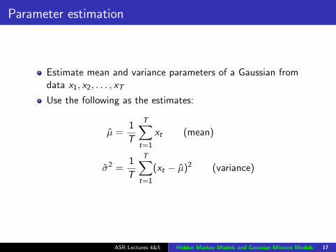
Parameter estimation
Estimate mean and variance parameters of a Gaussian fromdata x1, x2, . . . , xT
Use the following as the estimates:
µ =1
T
T∑t=1
xt (mean)
σ2 =1
T
T∑t=1
(xt − µ)2 (variance)
ASR Lectures 4&5 Hidden Markov Models and Gaussian Mixture Models 17

Exercise — maximum likelihood estimation (MLE)
Consider the log likelihood of a set of T training data points{x1, . . . , xT} being generated by a Gaussian with mean µ andvariance σ2:
L = ln p({x1, . . . , xT}|µ, σ2) = −1
2
T∑t=1
((xt − µ)2
σ2− lnσ2 − ln(2π)
)
= − 1
2σ2
T∑t=1
(xt − µ)2 − T
2lnσ2 − T
2ln(2π)
By maximising the the log likelihood function with respect to µshow that the maximum likelihood estimate for the mean is indeedthe sample mean:
µML =1
T
T∑t=1
xt .
ASR Lectures 4&5 Hidden Markov Models and Gaussian Mixture Models 18

The multivariate Gaussian distribution
The D-dimensional vector x = (x1, . . . , xD)T follows amultivariate Gaussian (or normal) distribution if it has aprobability density function of the following form:
p(x |µ,Σ) =1
(2π)D/2|Σ|1/2exp
(−1
2(x− µ)TΣ−1(x− µ)
)The pdf is parameterized by the mean vector µ = (µ1, . . . , µD)T
and the covariance matrix Σ =
σ11 . . . σ1D
.... . .
...σD1 . . . σDD
.The 1-dimensional Gaussian is a special case of this pdf
The argument to the exponential 0.5(x− µ)TΣ−1(x− µ) isreferred to as a quadratic form.
ASR Lectures 4&5 Hidden Markov Models and Gaussian Mixture Models 19

Covariance matrix
The mean vector µ is the expectation of x:
µ = E [x]
The covariance matrix Σ is the expectation of the deviation ofx from the mean:
Σ = E [(x− µ)(x− µ)T ]
Σ is a D × D symmetric matrix:
σij = E [(xi − µi )(xj − µj)] = E [(xj − µj)(xi − µi )] = σji
The sign of the covariance helps to determine the relationshipbetween two components:
If xj is large when xi is large, then (xi − µi )(xj − µj) will tendto be positive;If xj is small when xi is large, then (xi − µi )(xj − µj) will tendto be negative.
ASR Lectures 4&5 Hidden Markov Models and Gaussian Mixture Models 20

Spherical Gaussian
4
2
x1
0
Surface plot of p(x1, x
2)
-2
-4-4
-2
0
x2
2
4
0
0.02
0.04
0.06
0.08
0.1
0.12
0.14
0.16
p(x
1,x
2)
Contour plot of p(x1, x
2)
x1
-4 -3 -2 -1 0 1 2 3 4
x2
-4
-3
-2
-1
0
1
2
3
4
µ =
(00
)Σ =
(1 00 1
)ρ12 = 0
NB: Correlation coefficient ρij =σij√σiiσjj
(−1 ≤ ρij ≤ 1)
ASR Lectures 4&5 Hidden Markov Models and Gaussian Mixture Models 21
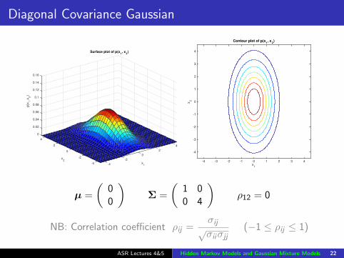
Diagonal Covariance Gaussian
4
2
x1
0
Surface plot of p(x1, x
2)
-2
-4-4
-2
0
x2
2
4
0
0.02
0.04
0.06
0.08
0.1
0.12
0.14
0.16
p(x
1,x
2)
Contour plot of p(x1, x
2)
x1
-4 -3 -2 -1 0 1 2 3 4
x2
-4
-3
-2
-1
0
1
2
3
4
µ =
(00
)Σ =
(1 00 4
)ρ12 = 0
NB: Correlation coefficient ρij =σij√σiiσjj
(−1 ≤ ρij ≤ 1)
ASR Lectures 4&5 Hidden Markov Models and Gaussian Mixture Models 22

Full covariance Gaussian
4
2
x1
0
Surface plot of p(x1, x
2)
-2
-4-4
-2
0
x2
2
4
0
0.02
0.04
0.06
0.08
0.16
0.14
0.12
0.1
p(x
1,x
2)
Contour plot of p(x1, x
2)
x1
-4 -3 -2 -1 0 1 2 3 4
x2
-4
-3
-2
-1
0
1
2
3
4
µ =
(00
)Σ =
(1 −1−1 4
)ρ12 = −0.5
NB: Correlation coefficient ρij =σij√σiiσjj
(−1 ≤ ρij ≤ 1)
ASR Lectures 4&5 Hidden Markov Models and Gaussian Mixture Models 23

Parameter estimation of a multivariate Gaussiandistribution
It is possible to show that the mean vector µ and covariancematrix Σ that maximize the likelihood of the training data aregiven by:
µ =1
T
T∑t=1
x t
Σ =1
T
T∑t=1
(x t − µ)(x t − µ)T
where x t = (xt1, . . . , xtD)T .
NB: T denotes either the number of samples or vectortranspose depending on context.
ASR Lectures 4&5 Hidden Markov Models and Gaussian Mixture Models 24
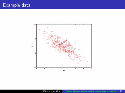
Example data
−4 −2 0 2 4 6 8 10−5
0
5
10
X1
X2
ASR Lectures 4&5 Hidden Markov Models and Gaussian Mixture Models 25
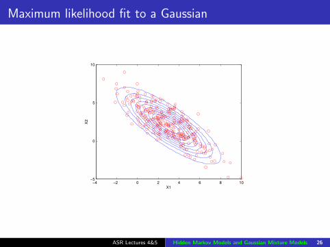
Maximum likelihood fit to a Gaussian
−4 −2 0 2 4 6 8 10−5
0
5
10
X1
X2
ASR Lectures 4&5 Hidden Markov Models and Gaussian Mixture Models 26

Data in clusters (example 1)
−1.5 −1 −0.5 0 0.5 1 1.5 2−1.5
−1
−0.5
0
0.5
1
1.5
2
2.5
µ1 = (0, 0)T µ2 = (1, 1)T Σ1 = Σ2 = 0.2 I
ASR Lectures 4&5 Hidden Markov Models and Gaussian Mixture Models 27

Example 1 fit by a Gaussian
−1.5 −1 −0.5 0 0.5 1 1.5 2−1.5
−1
−0.5
0
0.5
1
1.5
2
2.5
µ1 = (0, 0)T µ2 = (1, 1)T Σ1 = Σ2 = 0.2 I
ASR Lectures 4&5 Hidden Markov Models and Gaussian Mixture Models 28

k-means clustering
k-means is an automatic procedure for clustering unlabelleddata
Requires a prespecified number of clusters
Clustering algorithm chooses a set of clusters with theminimum within-cluster variance
Guaranteed to converge (eventually)
Clustering solution is dependent on the initialisation
ASR Lectures 4&5 Hidden Markov Models and Gaussian Mixture Models 29
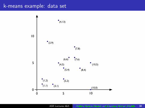
k-means example: data set
0 5 100
10
5
(1,1)
(1,2)
(3,1)
(4,5)
(5,2)
(5,4)
(6,6) (7,6)
(8,4)
(10,5)
(10,0)
(2,9)
(4,13)
(7,8)
ASR Lectures 4&5 Hidden Markov Models and Gaussian Mixture Models 30

k-means example: initialization
0 5 100
10
5
(1,1)
(1,2)
(3,1)
(4,5)
(5,2)
(5,4)
(6,6) (7,6)
(8,4)
(10,5)
(10,0)
(2,9)
(4,13)
(7,8)
ASR Lectures 4&5 Hidden Markov Models and Gaussian Mixture Models 31

k-means example: iteration 1 (assign points to clusters)
0 5 100
10
5
(1,1)
(1,2)
(3,1)
(4,5)
(5,2)
(5,4)
(6,6) (7,6)
(8,4)
(10,5)
(10,0)
(2,9)
(4,13)
(7,8)
ASR Lectures 4&5 Hidden Markov Models and Gaussian Mixture Models 32
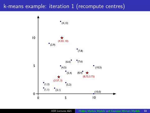
k-means example: iteration 1 (recompute centres)
0 5 100
10
5
(1,1)
(1,2)
(3,1)
(4,5)
(5,2)
(5,4)
(6,6) (7,6)
(8,4)
(10,5)
(10,0)
(2,9)
(4,13)
(7,8)
(4.33, 10)
(3.57, 3)
(8.75,3.75)
ASR Lectures 4&5 Hidden Markov Models and Gaussian Mixture Models 33

k-means example: iteration 2 (assign points to clusters)
0 5 100
10
5
(1,1)
(1,2)
(3,1)
(4,5)
(5,2)
(5,4)
(6,6) (7,6)
(8,4)
(10,5)
(10,0)
(2,9)
(4,13)
(7,8)
(4.33, 10)
(3.57, 3)
(8.75,3.75)
ASR Lectures 4&5 Hidden Markov Models and Gaussian Mixture Models 34

k-means example: iteration 2 (recompute centres)
0 5 100
10
5
(1,1)
(1,2)
(3,1)
(4,5)
(5,2)
(5,4)
(6,6) (7,6)
(8,4)
(10,5)
(10,0)
(2,9)
(4,13)
(7,8)
(4.33, 10)
(3.17, 2.5)
(8.2,4.2)
ASR Lectures 4&5 Hidden Markov Models and Gaussian Mixture Models 35
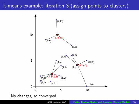
k-means example: iteration 3 (assign points to clusters)
0 5 100
10
5
(1,1)
(1,2)
(3,1)
(4,5)
(5,2)
(5,4)
(6,6) (7,6)
(8,4)
(10,5)
(10,0)
(2,9)
(4,13)
(7,8)
(4.33, 10)
(3.17, 2.5)
(8.2,4.2)
No changes, so converged
ASR Lectures 4&5 Hidden Markov Models and Gaussian Mixture Models 36
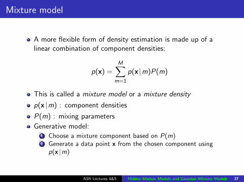
Mixture model
A more flexible form of density estimation is made up of alinear combination of component densities:
p(x) =M∑
m=1
p(x |m)P(m)
This is called a mixture model or a mixture density
p(x |m) : component densities
P(m) : mixing parameters
Generative model:1 Choose a mixture component based on P(m)2 Generate a data point x from the chosen component using
p(x |m)
ASR Lectures 4&5 Hidden Markov Models and Gaussian Mixture Models 37

Gaussian mixture model
The most important mixture model is the Gaussian Mixture Model(GMM), where the component densities are Gaussians
Consider a GMM, where each component Gaussian N (x;µm,Σm)has mean µm and a spherical covariance Σm = σ2m I
p(x) =M∑
m=1
P(m) p(x |m) =M∑
m=1
P(m)N (x;µm, σ2m I)
x1 x2 xd
p(x|1) p(x|2) p(x|M)
p(x)
P(1)P(2)
P(M)
ASR Lectures 4&5 Hidden Markov Models and Gaussian Mixture Models 38

GMM Parameter estimation when we know whichcomponent generated the data
Define the indicator variable zmt = 1 if component mgenerated data point x t (and 0 otherwise)
If zmt wasn’t hidden then we could count the number ofobserved data points generated by m:
Nm =T∑t=1
zmt
And estimate the mean, variance and mixing parameters as:
µm =
∑t zmtx t
Nm
σ2m =
∑t zmt‖x t−µm‖2
Nm
P(m) =1
T
∑t
zmt =Nm
T
ASR Lectures 4&5 Hidden Markov Models and Gaussian Mixture Models 39

GMM Parameter estimation when we don’t know whichcomponent generated the data
Problem: we don’t know which mixture component a datapoint comes from...
Idea: use the posterior probability P(m |x), which gives theprobability that component m was responsible for generatingdata point x.
P(m |x) =p(x |m)P(m)
p(x)=
p(x |m)P(m)∑Mm′=1 p(x |m′)P(m′)
The P(m |x)s are called the component occupationprobabilities (or sometimes called the responsibilities)
Since they are posterior probabilities:
M∑m=1
P(m |x) = 1
ASR Lectures 4&5 Hidden Markov Models and Gaussian Mixture Models 40

Soft assignment
Estimate “soft counts” based on the component occupationprobabilities P(m |x t):
N∗m =T∑t=1
P(m |x t)
We can imagine assigning data points to component mweighted by the component occupation probability P(m |x t)
So we could imagine estimating the mean, variance and priorprobabilities as:
µm =
∑t P(m |x t)x t∑t P(m |x t)
=
∑t P(m |x t)x t
N∗m
σ2m =
∑t P(m |x t) ‖x t−µm‖2∑
t P(m |x t)=
∑t P(m |x t) ‖x t−µm‖2
N∗m
P(m) =1
T
∑t
P(m |x t) =N∗mT
ASR Lectures 4&5 Hidden Markov Models and Gaussian Mixture Models 41

EM algorithm
Problem! Recall that:
P(m |x) =p(x |m)P(m)
p(x)=
p(x |m)P(m)∑Mm′=1 p(x |m′)P(m′)
We need to know p(x |m) and P(m) to estimate theparameters of P(m |x), and to estimate P(m)....Solution: an iterative algorithm where each iteration has twoparts:
Compute the component occupation probabilities P(m |x)using the current estimates of the GMM parameters (means,variances, mixing parameters) (E-step)Computer the GMM parameters using the current estimates ofthe component occupation probabilities (M-step)
Starting from some initialization (e.g. using k-means for themeans) these steps are alternated until convergence
This is called the EM Algorithm and can be shown tomaximize the likelihood
ASR Lectures 4&5 Hidden Markov Models and Gaussian Mixture Models 42
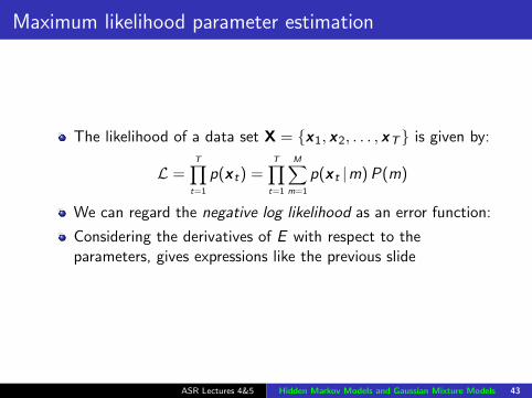
Maximum likelihood parameter estimation
The likelihood of a data set X = {x1, x2, . . . , xT} is given by:
L =T∏t=1
p(x t) =T∏t=1
M∑m=1
p(x t |m)P(m)
We can regard the negative log likelihood as an error function:
Considering the derivatives of E with respect to theparameters, gives expressions like the previous slide
ASR Lectures 4&5 Hidden Markov Models and Gaussian Mixture Models 43

Example 1 fit using a GMM
−1.5 −1 −0.5 0 0.5 1 1.5 2−1.5
−1
−0.5
0
0.5
1
1.5
2
2.5
Fitted with a two component GMM using EM
ASR Lectures 4&5 Hidden Markov Models and Gaussian Mixture Models 44

Peakily distributed data (Example 2)
−4 −3 −2 −1 0 1 2 3 4−5
−4
−3
−2
−1
0
1
2
3
4
µ1 = µ2 = [0 0]T Σ1 = 0.1I Σ2 = 2I
ASR Lectures 4&5 Hidden Markov Models and Gaussian Mixture Models 45

Example 2 fit by a Gaussian
−4 −3 −2 −1 0 1 2 3 4−5
−4
−3
−2
−1
0
1
2
3
4
µ1 = µ2 = [0 0]T Σ1 = 0.1I Σ2 = 2I
ASR Lectures 4&5 Hidden Markov Models and Gaussian Mixture Models 46

Example 2 fit by a GMM
−4 −3 −2 −1 0 1 2 3 4−5
−4
−3
−2
−1
0
1
2
3
4
Fitted with a two component GMM using EM
ASR Lectures 4&5 Hidden Markov Models and Gaussian Mixture Models 47

Example 2: component Gaussians
−4 −3 −2 −1 0 1 2 3 4−4
−3
−2
−1
0
1
2
3
4
−4 −3 −2 −1 0 1 2 3 4−4
−3
−2
−1
0
1
2
3
4
P(x |m=1) P(x |m=2)
ASR Lectures 4&5 Hidden Markov Models and Gaussian Mixture Models 48
Comments on GMMs
GMMs trained using the EM algorithm are able to selforganize to fit a data set
Individual components take responsibility for parts of the dataset (probabilistically)
Soft assignment to components not hard assignment — “softclustering”
GMMs scale very well, e.g.: large speech recognition systemscan have 30,000 GMMs, each with 32 components:sometimes 1 million Gaussian components!! And theparameters all estimated from (a lot of) data by EM
ASR Lectures 4&5 Hidden Markov Models and Gaussian Mixture Models 49
Back to HMMs...
s1 s2 s3 sEP(s2 | s1)
P(s2 | s2)
p(x | s2)
x
p(x | s1)
x x
P(s1|sI)
p(x | s3)
sIP(s3 | s2) P(sE | s3)
P(s3 | s3)P(s1 | s1)
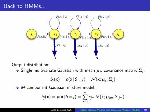
Output distribution:Single multivariate Gaussian with mean µj , covariance matrix Σj :
bj(x) = p(x |S = j) = N (x;µj ,Σj)
M-component Gaussian mixture model:
bj(x) = p(x |S = j) =M∑
m=1
cjmN (x;µjm,Σjm)
ASR Lectures 4&5 Hidden Markov Models and Gaussian Mixture Models 50
The three problems of HMMs
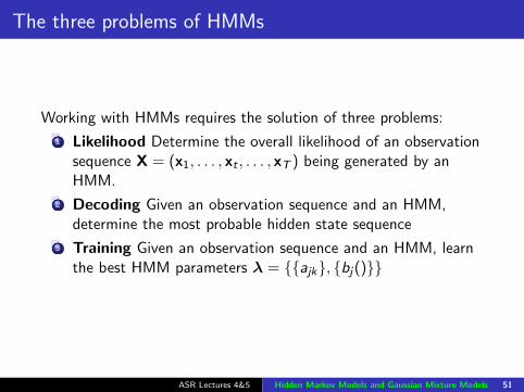
Working with HMMs requires the solution of three problems:
1 Likelihood Determine the overall likelihood of an observationsequence X = (x1, . . . , xt , . . . , xT ) being generated by anHMM.
2 Decoding Given an observation sequence and an HMM,determine the most probable hidden state sequence
3 Training Given an observation sequence and an HMM, learnthe best HMM parameters λ = {{ajk}, {bj()}}
ASR Lectures 4&5 Hidden Markov Models and Gaussian Mixture Models 51

1. Likelihood: how to calculate?
x1
S0
2
3
1
4
S
S
S
S
aa
a
a
a
a
01
12
2322
33 34
a11
764321 time5
x x3
x4
x5
x6
x72
observations
states
trellis
P(X,path` |λ) = P(X |path`,λ)P(path` |λ)= P(X |s0s1s1s1s2s2s3s3s4,λ)P(s0s1s1s1s2s2s3s3s4 |λ)= b1(x1)b1(x2)b1(x3)b2(x4)b2(x5)b3(x6)b3(x7)a01a11a11a12a22a23a33a34
P(X |λ) =∑{path`}
P(X,path` |λ) ' maxpath`
P(X, path` |λ)
forward(backward) algorithm Viterbi algorithm
ASR Lectures 4&5 Hidden Markov Models and Gaussian Mixture Models 52
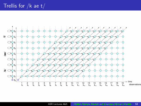
Trellis for /k ae t/
x
15x15 16x
16
17x
17
18x
18
19x
S0
x1
2
3
1
19observations
time
x 13x
13
12
1412
11x
11
10x
10
9
9
8x
8
S
1
3
2
1
3
2
S
S
S
S
S
S
S
S
7x72 6x5x4x3xx
51 2 3 4 6
14x
/k/
/ae/
/t/
ASR Lectures 4&5 Hidden Markov Models and Gaussian Mixture Models 53

1. Likelihood: The Forward algorithm
Goal: determine p(X |λ)
Sum over all possible state sequences s1s2 . . . sT that couldresult in the observation sequence XRather than enumerating each sequence, compute theprobabilities recursively (exploiting the Markov assumption)
Hown many paths calculations in p(X |λ)?
∼ N × N × · · ·N︸ ︷︷ ︸T times
= NT N : number of HMM statesT : length of observation
e.g. NT ≈ 1010 for N=3, T =20
Computation complexity of multiplication: O(2T NT )
The Forward algorithm reduces this to O(TN2)
ASR Lectures 4&5 Hidden Markov Models and Gaussian Mixture Models 54
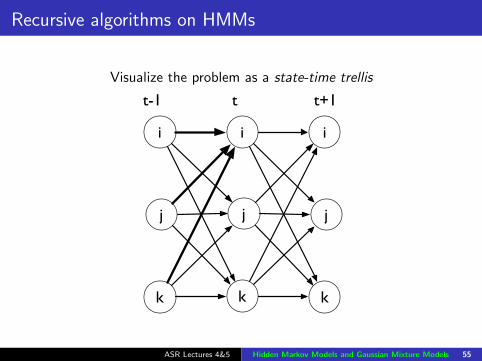
Recursive algorithms on HMMs
Visualize the problem as a state-time trellis
k
i
j
i
j
k
i
j
k
t-1 t t+1
ASR Lectures 4&5 Hidden Markov Models and Gaussian Mixture Models 55

1. Likelihood: The Forward algorithm
Goal: determine p(X |λ)
Sum over all possible state sequences s1s2 . . . sT that couldresult in the observation sequence XRather than enumerating each sequence, compute theprobabilities recursively (exploiting the Markov assumption)
Forward probability, αt( j ): the probability of observing theobservation sequence x1 . . . xt and being in state j at time t:
αt( j ) = p(x1, . . . , xt ,S(t)= j |λ)
ASR Lectures 4&5 Hidden Markov Models and Gaussian Mixture Models 56
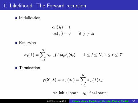
1. Likelihood: The Forward recursion
Initialization
α0(sI ) = 1
α0( j ) = 0 if j 6= sI
Recursion
αt( j ) =N∑i=1
αt−1( i )aijbj(xt) 1 ≤ j ≤ N, 1 ≤ t ≤ T
Termination
p(X |λ) = αT (sE ) =N∑i=1
αT ( i )aiE
sI : initial state, sE : final state
ASR Lectures 4&5 Hidden Markov Models and Gaussian Mixture Models 57
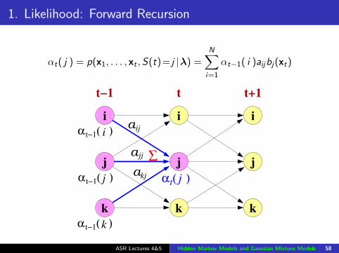
1. Likelihood: Forward Recursion
αt( j ) = p(x1, . . . , xt ,S(t)= j |λ) =N∑i=1
αt−1( i )aijbj(xt)
t−1
t
t−1
t−1 jj
k
i
kj
jj
ij
k
j
i
t+1
α ( )
α ( )
α ( )
Σ
a
α ( )
a
a
k
j
i
k
j
i
tt−1
ASR Lectures 4&5 Hidden Markov Models and Gaussian Mixture Models 58
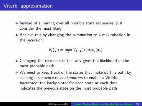
Viterbi approximation
Instead of summing over all possible state sequences, justconsider the most likely
Achieve this by changing the summation to a maximisation inthe recursion:
Vt( j ) = maxi
Vt−1( i )aijbj(xt)
Changing the recursion in this way gives the likelihood of themost probable path
We need to keep track of the states that make up this path bykeeping a sequence of backpointers to enable a Viterbibacktrace: the backpointer for each state at each timeindicates the previous state on the most probable path
ASR Lectures 4&5 Hidden Markov Models and Gaussian Mixture Models 59
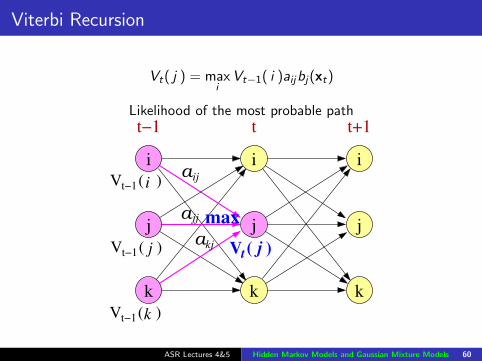
Viterbi Recursion
Vt( j ) = maxi
Vt−1( i )aijbj(xt)
Likelihood of the most probable path
t−1
t−1 t
t−1
j
jj
kjj
i
k
ij
ia
j
k
V ( )
V ( )
max
V ( ) V ( )
i
a
a
t t+1t−1
i
j
k k
j
ASR Lectures 4&5 Hidden Markov Models and Gaussian Mixture Models 60

Viterbi Recursion
Backpointers to the previous state on the most probable path
t−1
t
t−1
t
t−1ij
jjj
j jkj
i
k
i
aV ( )
V ( )
bt ( )=
V ( ) V ( )
k
a
a
t t+1t−1
i
j
k k
j
i i
j
ASR Lectures 4&5 Hidden Markov Models and Gaussian Mixture Models 61

2. Decoding: The Viterbi algorithm
Initialization
V0( i ) = 1
V0( j ) = 0 if j 6= i
bt0( j ) = 0
Recursion
Vt( j ) =N
maxi=1
Vt−1( i )aijbj(xt)
btt( j ) = argN
maxi=1
Vt−1( i )aijbj(xt)
Termination
P∗ = VT (sE ) =N
maxi=1
VT ( i )aiE
s∗T = btT (qE ) = argN
maxi=1
VT ( i )aiE
ASR Lectures 4&5 Hidden Markov Models and Gaussian Mixture Models 62
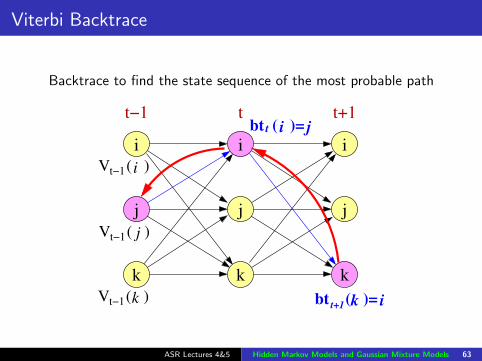
Viterbi Backtrace
Backtrace to find the state sequence of the most probable path
t−1
t+1
t
t−1
t−1
j
i
k
ji
ik
i
k
V ( )
i
t−1 t+1
V ( )
i
j
bt ( )=
bt ( )=
V ( )
t
j
k k
j
ASR Lectures 4&5 Hidden Markov Models and Gaussian Mixture Models 63

3. Training: Forward-Backward algorithm
Goal: Efficiently estimate the parameters of an HMM λ froman observation sequence
Assume single Gaussian output probability distribution
bj(x) = p(x | j ) = N (x;µj ,Σj)
Parameters λ:
Transition probabilities aij :∑j
aij = 1
Gaussian parameters for state j :mean vector µj ; covariance matrix Σj
ASR Lectures 4&5 Hidden Markov Models and Gaussian Mixture Models 64

Viterbi Training
If we knew the state-time alignment, then each observationfeature vector could be assigned to a specific stateA state-time alignment can be obtained using the mostprobable path obtained by Viterbi decodingMaximum likelihood estimate of aij , if C ( i → j ) is the countof transitions from i to j
aij =C ( i → j )∑k C ( i → k )
Likewise if Zj is the set of observed acoustic feature vectorsassigned to state j , we can use the standard maximumlikelihood estimates for the mean and the covariance:
µj =
∑x∈Zj
x
|Zj |
Σj =
∑x∈Zj
(x − µj)(x − µj)T
|Zj |ASR Lectures 4&5 Hidden Markov Models and Gaussian Mixture Models 65

EM Algorithm
Viterbi training is an approximation—we would like toconsider all possible paths
In this case rather than having a hard state-time alignment weestimate a probability
State occupation probability: The probability γt( j ) ofoccupying state j at time t given the sequence ofobservations.Compare with component occupation probability in a GMM
We can use this for an iterative algorithm for HMM training:the EM algorithm (whose adaption to HMM is called ’Baum-Welch algorithm’)
Each iteration has two steps:
E-step estimate the state occupation probabilities(Expectation)
M-step re-estimate the HMM parameters based on theestimated state occupation probabilities(Maximisation)
ASR Lectures 4&5 Hidden Markov Models and Gaussian Mixture Models 66

Backward probabilities
To estimate the state occupation probabilities it is useful todefine (recursively) another set of probabilities—the Backwardprobabilities
βt( j ) = p(xt+1, . . . , xT |S(t)= j ,λ)
The probability of future observations given a the HMM is instate j at time tThese can be recursively computed (going backwards in time)
InitialisationβT ( i ) = aiE
Recursion
βt( i ) =N∑j=1
aijbj(xt+1)βt+1( j ) for t = T−1, . . . , 1
Termination
p(X |λ) = β0( I ) =N∑j=1
aIjbj(x1)β1( j ) = αT (sE )
ASR Lectures 4&5 Hidden Markov Models and Gaussian Mixture Models 67

Backward Recursion
βt( j ) = p(xt+1, . . . , xT |S(t)= j ,λ) =N∑j=1
aijbj(xt+1)βt+1( j )
t+1
t+1
t+1
tjk
ji
jj
i
j
k
j
Σ
a
k
j
i
k
j
i
tt−1
k
j
i
t+1
β ( )
β ( )
β ( )
β ( )
a
a
ASR Lectures 4&5 Hidden Markov Models and Gaussian Mixture Models 68
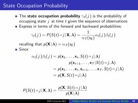
State Occupation Probability
The state occupation probability γt( j ) is the probability ofoccupying state j at time t given the sequence of observationsExpress in terms of the forward and backward probabilities:
γt( j ) = P(S(t)= j |X,λ) =1
αT (sE )αt( j )βt( j )
recalling that p(X |λ) = αT (sE )Since
αt( j )βt( j ) = p(x1, . . . , xt , S(t)= j |λ)
p(xt+1, . . . , xT |S(t)= j ,λ)
= p(x1, . . . , xt , xt+1, . . . , xT ,S(t)= j |λ)
= p(X,S(t)= j |λ)
P(S(t)= j |X,λ) =p(X, S(t)= j |λ)
p(X |λ)
ASR Lectures 4&5 Hidden Markov Models and Gaussian Mixture Models 69

Re-estimation of Gaussian parameters
The sum of state occupation probabilities through time for astate, may be regarded as a “soft” count
We can use this “soft” alignment to re-estimate the HMMparameters:
µj =
∑Tt=1 γt( j )x t∑Tt=1 γt( j )
Σj =
∑Tt=1 γt( j )(x t − µj)(x − µj)
T∑Tt=1 γt( j )
ASR Lectures 4&5 Hidden Markov Models and Gaussian Mixture Models 70

Re-estimation of transition probabilities
Similarly to the state occupation probability, we can estimateξt( i , j ), the probability of being in i at time t and j att + 1, given the observations:
ξt( i , j ) = P(S(t)= i , S(t+1)= j |X,λ)
=p(S(t)= i ,S(t+1)= j ,X |λ)
p(X |λ)
=αt( i )aijbj(xt+1)βt+1( j )
αT (sE )
We can use this to re-estimate the transition probabilities
aij =
∑Tt=1 ξt( i , j )∑N
k=1
∑Tt=1 ξt( i , k )
ASR Lectures 4&5 Hidden Markov Models and Gaussian Mixture Models 71

Pulling it all together
Iterative estimation of HMM parameters using the EMalgorithm. At each iteration
E step For all time-state pairs1 Recursively compute the forward probabilitiesαt( j ) and backward probabilities βt( j )
2 Compute the state occupation probabilitiesγt( j ) and ξt( i , j )
M step Based on the estimated state occupationprobabilities re-estimate the HMM parameters:mean vectors µj , covariance matrices Σj andtransition probabilities aij
The application of the EM algorithm to HMM training issometimes called the Forward-Backward algorithm
ASR Lectures 4&5 Hidden Markov Models and Gaussian Mixture Models 72
Extension to a corpus of utterances
We usually train from a large corpus of R utterances
If xrt is the t th frame of the r th utterance Xr then we cancompute the probabilities αr
t( j ), βrt ( j ), γrt ( j ) and ξrt ( i , j )as before
The re-estimates are as before, except we must sum over theR utterances, eg:
µj =
∑Rr=1
∑Tt=1 γ
rt ( j )x r
t∑Rr=1
∑Tt=1 γ
rt ( j )
In addition, we usually employ “embedded training”, in whichfine tuning of phone labelling with “forced Viterbi alignment”or forced alignment is involved. (For details see Section 9.7 inJurafsky and Martin’s SLP)
ASR Lectures 4&5 Hidden Markov Models and Gaussian Mixture Models 73

Extension to Gaussian mixture model (GMM)
The assumption of a Gaussian distribution at each state isvery strong; in practice the acoustic feature vectors associatedwith a state may be strongly non-Gaussian
In this case an M-component Gaussian mixture model is anappropriate density function:
bj(x) = p(x |S = j) =M∑
m=1
cjmN (x;µjm,Σjm)
Given enough components, this family of functions can modelany distribution.
Train using the EM algorithm, in which the componentestimation probabilities are estimated in the E-step
ASR Lectures 4&5 Hidden Markov Models and Gaussian Mixture Models 75
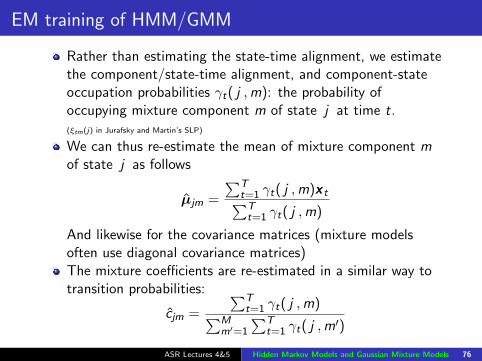
EM training of HMM/GMM
Rather than estimating the state-time alignment, we estimatethe component/state-time alignment, and component-stateoccupation probabilities γt( j ,m): the probability ofoccupying mixture component m of state j at time t.(ξtm(j) in Jurafsky and Martin’s SLP)
We can thus re-estimate the mean of mixture component mof state j as follows
µjm =
∑Tt=1 γt( j ,m)x t∑Tt=1 γt( j ,m)
And likewise for the covariance matrices (mixture modelsoften use diagonal covariance matrices)The mixture coefficients are re-estimated in a similar way totransition probabilities:
cjm =
∑Tt=1 γt( j ,m)∑M
m′=1
∑Tt=1 γt( j ,m
′)
ASR Lectures 4&5 Hidden Markov Models and Gaussian Mixture Models 76
Doing the computation
The forward, backward and Viterbi recursions result in a longsequence of probabilities being multiplied
This can cause floating point underflow problems
In practice computations are performed in the log domain (inwhich multiplies become adds)
Working in the log domain also avoids needing to perform theexponentiation when computing Gaussians
ASR Lectures 4&5 Hidden Markov Models and Gaussian Mixture Models 77

A note on HMM topology
ergodic modelleft−to−right model parallel path left−to−right model
a11 a12 00 a22 a230 0 a33
a11 a12 a13 0 00 a22 a23 a24 00 0 a33 a34 a350 0 0 a44 a450 0 0 0 a55
a11 a12 a13 a14 a15a21 a22 a23 a24 a25a31 a32 a33 a34 a35a41 a42 a43 a44 a45a51 a52 a53 a54 a55
Speech recognition: left-to-right HMM with 3 ∼ 5 statesSpeaker recognition: ergodic HMM
ASR Lectures 4&5 Hidden Markov Models and Gaussian Mixture Models 78

A note on HMM emission probabilities
31
2
22a
11
23 34a
b (x)
a
a12
a
b (x) b (x)
01a
33a
emission pdfs
Emission prob.
Continuous (density) HMM continuous density GMM, NN/DNNDiscrete (probability) HMM discrete probability VQ
Semi-continuous HMM continuous density tied mixture(tied-mixture HMM)
ASR Lectures 4&5 Hidden Markov Models and Gaussian Mixture Models 79
Summary: HMMs
HMMs provide a generative model for statistical speechrecognition
Three key problems1 Computing the overall likelihood: the Forward algorithm2 Decoding the most likely state sequence: the Viterbi algorithm3 Estimating the most likely parameters: the EM
(Forward-Backward) algorithm
Solutions to these problems are tractable due to the two keyHMM assumptions
1 Conditional independence of observations given the currentstate
2 Markov assumption on the states
ASR Lectures 4&5 Hidden Markov Models and Gaussian Mixture Models 80
References: HMMs
Gales and Young (2007). “The Application of Hidden MarkovModels in Speech Recognition”, Foundations and Trends inSignal Processing, 1 (3), 195–304: section 2.2.
Jurafsky and Martin (2008). Speech and Language Processing(2nd ed.): sections 6.1–6.5; 9.2; 9.4. (Errata athttp://www.cs.colorado.edu/~martin/SLP/Errata/
SLP2-PIEV-Errata.html)
Rabiner and Juang (1989). “An introduction to hiddenMarkov models”, IEEE ASSP Magazine, 3 (1), 4–16.
Renals and Hain (2010). “Speech Recognition”,Computational Linguistics and Natural Language ProcessingHandbook, Clark, Fox and Lappin (eds.), Blackwells.
ASR Lectures 4&5 Hidden Markov Models and Gaussian Mixture Models 81