hidden markov model cryptanalysis - uni-saarland.de · introduction randomized algorithms input...
TRANSCRIPT
Introduction Randomized Algorithms Input Driven Hidden Markov Models Analysis of the Oswald Aigner Randomizations Conclusion
Hidden Markov Model CryptanalysisC. Karlof, D. Wagner
presented by: Stephan Neumann
January 23th, 2009

Introduction Randomized Algorithms Input Driven Hidden Markov Models Analysis of the Oswald Aigner Randomizations Conclusion
Outline
1 IntroductionMotivationAttacker Model
2 Randomized AlgorithmsBinary algorithm for scalar multiplicationRandomized binary algorithm for scalar multiplication
3 Input Driven Hidden Markov ModelsDefinitionKey Inference ProblemKey Inference Problem Approaches
4 Analysis of the Oswald Aigner RandomizationsOswald Aigner RandomizationResults
5 Conclusion
Introduction Randomized Algorithms Input Driven Hidden Markov Models Analysis of the Oswald Aigner Randomizations Conclusion
Motivation
Motivation
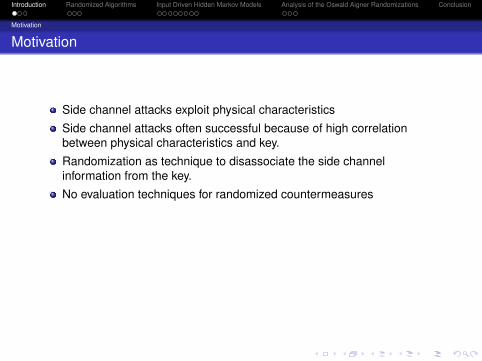
Side channel attacks exploit physical characteristics
Side channel attacks often successful because of high correlationbetween physical characteristics and key.
Randomization as technique to disassociate the side channelinformation from the key.
No evaluation techniques for randomized countermeasures
Goal of the paper
Evaluation technique for randomized countermeasures against side channelattacks

Introduction Randomized Algorithms Input Driven Hidden Markov Models Analysis of the Oswald Aigner Randomizations Conclusion
Motivation
Motivation
Side channel attacks exploit physical characteristics
Side channel attacks often successful because of high correlationbetween physical characteristics and key.
Randomization as technique to disassociate the side channelinformation from the key.
No evaluation techniques for randomized countermeasures
Goal of the paper
Evaluation technique for randomized countermeasures against side channelattacks
Introduction Randomized Algorithms Input Driven Hidden Markov Models Analysis of the Oswald Aigner Randomizations Conclusion
Attacker Model
The Attacker
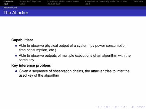
Capabilities:Able to observe physical output of a system (by power consumption,time consumption, etc.)
Able to observe outputs of multiple executions of an algorithm with thesame key
Key inference problem:Given a sequence of observation chains, the attacker tries to infer theused key of the algorithm

Introduction Randomized Algorithms Input Driven Hidden Markov Models Analysis of the Oswald Aigner Randomizations Conclusion
Attacker Model
General Approach
1 Develop generic side channel attack against randomized algorithms2 Apply attack to randomized countermeasures against side channel
attacks
Interpretation
A countermeasure is good if the attack performs poorly

Introduction Randomized Algorithms Input Driven Hidden Markov Models Analysis of the Oswald Aigner Randomizations Conclusion
Outline
1 IntroductionMotivationAttacker Model
2 Randomized AlgorithmsBinary algorithm for scalar multiplicationRandomized binary algorithm for scalar multiplication
3 Input Driven Hidden Markov ModelsDefinitionKey Inference ProblemKey Inference Problem Approaches
4 Analysis of the Oswald Aigner RandomizationsOswald Aigner RandomizationResults
5 Conclusion

Introduction Randomized Algorithms Input Driven Hidden Markov Models Analysis of the Oswald Aigner Randomizations Conclusion
Binary algorithm for scalar multiplication
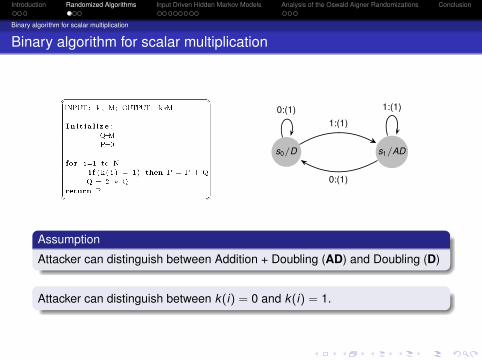
Binary algorithm for scalar multiplication
s0/D s1/AD
0:(1)1:(1)
1:(1)
0:(1)
Assumption
Attacker can distinguish between Addition + Doubling (AD) and Doubling (D)
Attacker can distinguish between k(i) = 0 and k(i) = 1.

Introduction Randomized Algorithms Input Driven Hidden Markov Models Analysis of the Oswald Aigner Randomizations Conclusion
Binary algorithm for scalar multiplication
Binary algorithm for scalar multiplication
s0/D s1/AD
0:(1)1:(1)
1:(1)
0:(1)
Assumption
Attacker can distinguish between Addition + Doubling (AD) and Doubling (D)
Attacker can distinguish between k(i) = 0 and k(i) = 1.

Introduction Randomized Algorithms Input Driven Hidden Markov Models Analysis of the Oswald Aigner Randomizations Conclusion
Randomized binary algorithm for scalar multiplication
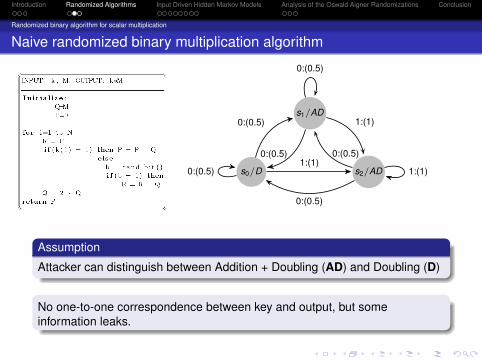
Naive randomized binary multiplication algorithm
s0/D
s1/AD
s2/AD0:(0.5)
0:(0.5)
1:(1)
0:(0.5)
0:(0.5)
1:(1)
1:(1)
0:(0.5)
0:(0.5)
Assumption
Attacker can distinguish between Addition + Doubling (AD) and Doubling (D)
No one-to-one correspondence between key and output, but someinformation leaks.

Introduction Randomized Algorithms Input Driven Hidden Markov Models Analysis of the Oswald Aigner Randomizations Conclusion
Randomized binary algorithm for scalar multiplication
Naive randomized binary multiplication algorithm
s0/D
s1/AD
s2/AD0:(0.5)
0:(0.5)
1:(1)
0:(0.5)
0:(0.5)
1:(1)
1:(1)
0:(0.5)
0:(0.5)
Assumption
Attacker can distinguish between Addition + Doubling (AD) and Doubling (D)
No one-to-one correspondence between key and output
, but someinformation leaks.
Introduction Randomized Algorithms Input Driven Hidden Markov Models Analysis of the Oswald Aigner Randomizations Conclusion
Randomized binary algorithm for scalar multiplication
Naive randomized binary multiplication algorithm
s0/D
s1/AD
s2/AD0:(0.5)
0:(0.5)
1:(1)
0:(0.5)
0:(0.5)
1:(1)
1:(1)
0:(0.5)
0:(0.5)
Assumption
Attacker can distinguish between Addition + Doubling (AD) and Doubling (D)
No one-to-one correspondence between key and output, but someinformation leaks.
Introduction Randomized Algorithms Input Driven Hidden Markov Models Analysis of the Oswald Aigner Randomizations Conclusion
Randomized binary algorithm for scalar multiplication
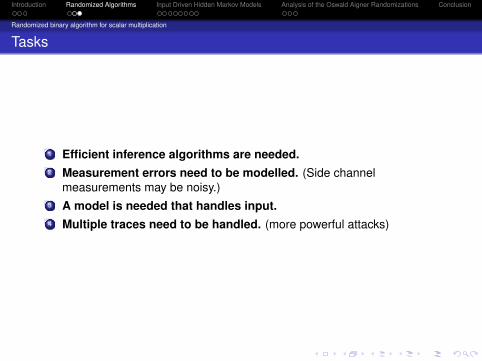
Tasks
1 Efficient inference algorithms are needed.2 Measurement errors need to be modelled. (Side channel
measurements may be noisy.)3 A model is needed that handles input.4 Multiple traces need to be handled. (more powerful attacks)

Introduction Randomized Algorithms Input Driven Hidden Markov Models Analysis of the Oswald Aigner Randomizations Conclusion
Outline
1 IntroductionMotivationAttacker Model
2 Randomized AlgorithmsBinary algorithm for scalar multiplicationRandomized binary algorithm for scalar multiplication
3 Input Driven Hidden Markov ModelsDefinitionKey Inference ProblemKey Inference Problem Approaches
4 Analysis of the Oswald Aigner RandomizationsOswald Aigner RandomizationResults
5 Conclusion

Introduction Randomized Algorithms Input Driven Hidden Markov Models Analysis of the Oswald Aigner Randomizations Conclusion
Definition
Input Driven Hidden Markov Model
Definition
A Input Driven Hidden Markov Model is a septuple
M = (S, I, O, A, B, C, s0)
S: finite set of internal statesI: finite set of input symbolsO: finite set of symbols that represent operations observable over the sidechannelA : |S|× |I|× |S| transition matrix where Aijk = Pr [Q l
n = sk |Q ln−1 = si , Kn = kj ]
B : |S| × |O| output matrix where Bij = Pr [Y ln = oj |Q l
n = si ]D : n × |I| key distribution matrix where Cjk = Pr [Kj = ik ]s0 ∈ S: initial state
Note
Probabilistic finite state machines can be transformed into Input DrivenHidden Markov Models in a straight-forward manner.
Introduction Randomized Algorithms Input Driven Hidden Markov Models Analysis of the Oswald Aigner Randomizations Conclusion
Key Inference Problem
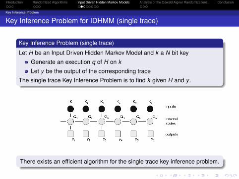
Key Inference Problem for IDHMM (single trace)
Key Inference Problem (single trace)
Let H be an Input Driven Hidden Markov Model and k a N bit key
Generate an execution q of H on k
Let y be the output of the corresponding trace
The single trace Key Inference Problem is to find k given H and y .
There exists an efficient algorithm for the single trace key inference problem.
Introduction Randomized Algorithms Input Driven Hidden Markov Models Analysis of the Oswald Aigner Randomizations Conclusion
Key Inference Problem
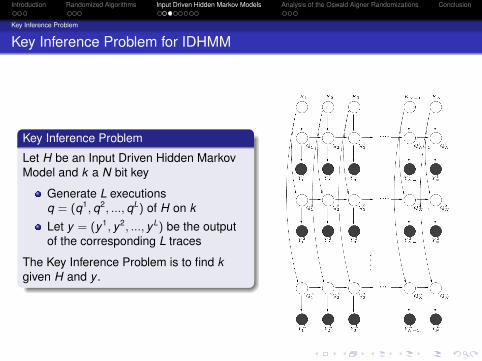
Key Inference Problem for IDHMM
Key Inference Problem
Let H be an Input Driven Hidden MarkovModel and k a N bit key
Generate L executionsq = (q1, q2, ..., qL) of H on k
Let y = (y1, y2, ..., yL) be the outputof the corresponding L traces
The Key Inference Problem is to find kgiven H and y .
Introduction Randomized Algorithms Input Driven Hidden Markov Models Analysis of the Oswald Aigner Randomizations Conclusion
Key Inference Problem Approaches
Key Inference Problem for IDHMM
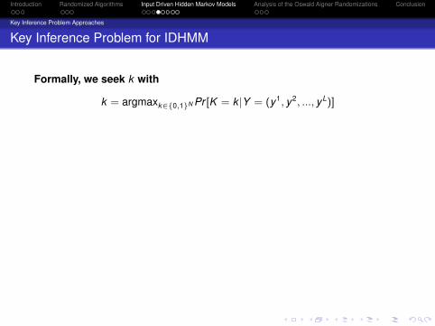
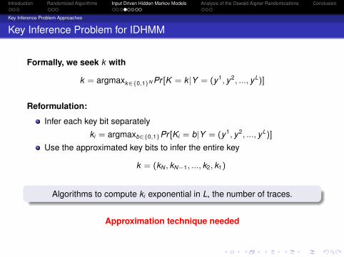
Formally, we seek k with
k = argmaxk∈{0,1}N Pr [K = k |Y = (y1, y2, ..., yL)]
Reformulation:
Infer each key bit separately
ki = argmaxb∈{0,1}Pr [Ki = b|Y = (y1, y2, ..., yL)]
Use the approximated key bits to infer the entire key
k = (kN , kN−1, ..., k2, k1)
Algorithms to compute ki exponential in L, the number of traces.
Approximation technique needed

Introduction Randomized Algorithms Input Driven Hidden Markov Models Analysis of the Oswald Aigner Randomizations Conclusion
Key Inference Problem Approaches
Key Inference Problem for IDHMM
Formally, we seek k with
k = argmaxk∈{0,1}N Pr [K = k |Y = (y1, y2, ..., yL)]
Reformulation:
Infer each key bit separately
ki = argmaxb∈{0,1}Pr [Ki = b|Y = (y1, y2, ..., yL)]
Use the approximated key bits to infer the entire key
k = (kN , kN−1, ..., k2, k1)
Algorithms to compute ki exponential in L, the number of traces.
Approximation technique needed

Introduction Randomized Algorithms Input Driven Hidden Markov Models Analysis of the Oswald Aigner Randomizations Conclusion
Key Inference Problem Approaches
Belief propagation
Idea
Reduce the multiple trace key inference problem to L single trace inferenceproblems, thereby improving the key distribution approximation
In the processing of a trace, the trace and the prior distribution are usedto compute the new key distribution
Dj = Pr [ki = 1|yj , Dj−1]
Introduction Randomized Algorithms Input Driven Hidden Markov Models Analysis of the Oswald Aigner Randomizations Conclusion
Key Inference Problem Approaches
Belief propagation cont’d
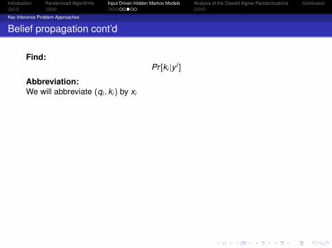
Find:Pr [ki |y j ]
Abbreviation:We will abbreviate (qi , ki) by xi
We set:
f (x0, ..., xN) = Pr [x0, ..., xN , y j ] =NY
n=1
gn(xn−1, xn)
whereg1(x0, x1) = Pr [x0] · Pr [x1|x0] · Pr [y j
1|x1]
gn(xn−1, xn) = Pr [xn|xn−1] · Pr [y jn|xn]
and
ti(xi) =P
x0...
Pxi−1
Pxi+1
...P
xNf (x0, ..., xN)
= Pr [xi , y j ]

Introduction Randomized Algorithms Input Driven Hidden Markov Models Analysis of the Oswald Aigner Randomizations Conclusion
Key Inference Problem Approaches
Belief propagation cont’d
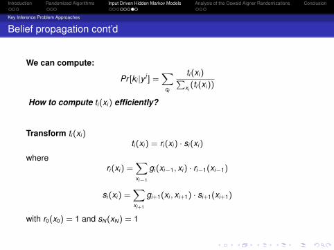
We can compute:
Pr [ki |y j ] =X
qi
ti(xi)Pxi(ti(xi))
How to compute ti(xi) efficiently?
Transform ti(xi)ti(xi) = ri(xi) · si(xi)
whereri(xi) =
Xxi−1
gi(xi−1, xi) · ri−1(xi−1)
si(xi) =Xxi+1
gi+1(xi , xi+1) · si+1(xi+1)
with r0(x0) = 1 and sN(xN) = 1
Introduction Randomized Algorithms Input Driven Hidden Markov Models Analysis of the Oswald Aigner Randomizations Conclusion
Key Inference Problem Approaches
Belief propagation cont’d
We can compute:
Pr [ki |y j ] =X
qi
ti(xi)Pxi(ti(xi))
How to compute ti(xi) efficiently?
Transform ti(xi)ti(xi) = ri(xi) · si(xi)
whereri(xi) =
Xxi−1
gi(xi−1, xi) · ri−1(xi−1)
si(xi) =Xxi+1
gi+1(xi , xi+1) · si+1(xi+1)
with r0(x0) = 1 and sN(xN) = 1
Introduction Randomized Algorithms Input Driven Hidden Markov Models Analysis of the Oswald Aigner Randomizations Conclusion
Key Inference Problem Approaches
Key Inference Problem for IDHMM cont’d
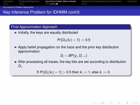
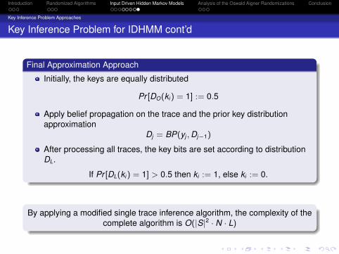
Final Approximation Approach
Initially, the keys are equally distributed
Pr [DO(ki) = 1] := 0.5
Apply belief propagation on the trace and the prior key distributionapproximation
Dj = BP(yj , Dj−1)
After processing all traces, the key bits are set according to distributionDL.
If Pr [DL(ki) = 1] > 0.5 then ki := 1, else ki := 0.
By applying a modified single trace inference algorithm, the complexity of thecomplete algorithm is O(|S|2 · N · L)
Introduction Randomized Algorithms Input Driven Hidden Markov Models Analysis of the Oswald Aigner Randomizations Conclusion
Key Inference Problem Approaches
Key Inference Problem for IDHMM cont’d
Final Approximation Approach
Initially, the keys are equally distributed
Pr [DO(ki) = 1] := 0.5
Apply belief propagation on the trace and the prior key distributionapproximation
Dj = BP(yj , Dj−1)
After processing all traces, the key bits are set according to distributionDL.
If Pr [DL(ki) = 1] > 0.5 then ki := 1, else ki := 0.
By applying a modified single trace inference algorithm, the complexity of thecomplete algorithm is O(|S|2 · N · L)
Introduction Randomized Algorithms Input Driven Hidden Markov Models Analysis of the Oswald Aigner Randomizations Conclusion
Outline
1 IntroductionMotivationAttacker Model
2 Randomized AlgorithmsBinary algorithm for scalar multiplicationRandomized binary algorithm for scalar multiplication
3 Input Driven Hidden Markov ModelsDefinitionKey Inference ProblemKey Inference Problem Approaches
4 Analysis of the Oswald Aigner RandomizationsOswald Aigner RandomizationResults
5 Conclusion

Introduction Randomized Algorithms Input Driven Hidden Markov Models Analysis of the Oswald Aigner Randomizations Conclusion
Oswald Aigner Randomization
Oswald Aigner Randomized Algorithms
Basis:Earlier presented binary scalar multiplication algorithm
Morain Olivos transformations
Morain Olivos transformations
If a multiplication factor k contains blocks of the form 01a or 01a01b, thecorresponding factor parts are transformed as follows:
01a 7→ 10a−11 (MO1)
01a01b 7→ 10a10b−11 (MO2)
Algorithms:
Oswald Aigner Randomized Algorithms
If transformation MO1 (resp. MO2) is applicable to key k within multiplicationk ·M, a coin is flipped if MO1 (resp. MO2) is applied to k .

Introduction Randomized Algorithms Input Driven Hidden Markov Models Analysis of the Oswald Aigner Randomizations Conclusion
Oswald Aigner Randomization
Oswald Aigner Randomization (OA1)
Figure: Randomized state machine representing the OA1 binary scalar multiplicationalgorithm

Introduction Randomized Algorithms Input Driven Hidden Markov Models Analysis of the Oswald Aigner Randomizations Conclusion
Results
Results of the Attacks against OA1 and OA2
The following table shows the results of the attack against the OA1 and OA2algorithms using a 192 bit key.
Remark
Results highly depending on the order of the processed traces

Introduction Randomized Algorithms Input Driven Hidden Markov Models Analysis of the Oswald Aigner Randomizations Conclusion
Outline
1 IntroductionMotivationAttacker Model
2 Randomized AlgorithmsBinary algorithm for scalar multiplicationRandomized binary algorithm for scalar multiplication
3 Input Driven Hidden Markov ModelsDefinitionKey Inference ProblemKey Inference Problem Approaches
4 Analysis of the Oswald Aigner RandomizationsOswald Aigner RandomizationResults
5 Conclusion

Introduction Randomized Algorithms Input Driven Hidden Markov Models Analysis of the Oswald Aigner Randomizations Conclusion
Conclusion
Contribution of the paper:Introduction of Hidden Markov Models as generic evaluation techniquefor randomized countermeasures
Belief propagation as reasonable approximation to handle the multipletrace key inference problem complexity
Integration of output observation errors
The randomized algorithms proposed by Oswald and Aigner failcompletely
Introduction Randomized Algorithms Input Driven Hidden Markov Models Analysis of the Oswald Aigner Randomizations Conclusion
References
C. Karlof, D. Wagner. Hidden Markov model cryptanalysis., InCryptographic Hardware and Embedded Systems – CHES 2003,Springer-Verlag LNCS 2779, 17–34, 2003
P.J Green, R. Noad, N.P. Smart. Further Hidden Markov ModelCryptanalysis, In Cryptographic Hardware and Embedded Systems -CHES 2005, 61-74
F. Morain, J. Olivos. Speeding up the computation on an ellipticcurve using addition-subtraction chains., Inform. Theory Appl. 24(1990), 531-543
E. Oswald, M. Aigner. Randomized addition-subtraction chains as acounter- measure against power attacks., In Cryptographic Hardwareand Embedded Systems – CHES 2001, Springer-Verlag LNCS 2162,39–50, 2001.
E. Oswald. Side-Channel Analysis., In Advances in Elliptic Curve Cryp-tography. Cambridge University Press, 69–86, 2005.