heteroclinic tangles and homoclinic snaking in the unfolding of a degenerate reversible...

Physica D 129 (1999) 147–170

Heteroclinic tangles and homoclinic snaking in the unfolding of adegenerate reversible Hamiltonian–Hopf bifurcation

P.D. Woods, A.R. Champneys∗Department of Engineering Mathematics, University of Bristol, Bristol BS8 1TR, UK

Received 24 July 1998; received in revised form 23 November 1998; accepted 25 November 1998Communicated by C.K.R.T. Jones

Abstract

This paper considers an unfolding of a degenerate reversible 1–1 resonance (or Hamiltonian–Hopf) bifurcation for four-dimensional systems of time reversible ordinary differential equations (ODEs). This bifurcation occurs when a complexquadruple of eigenvalues of an equilibrium coalesce on the imaginary axis to become imaginary pairs. The degeneracy occursvia the vanishing of a normal form coefficient(q2 = 0) that determines whether the bifurcation is super- or subcritical. Ofparticular concern is the behaviour of homoclinic and heteroclinic connections between the trivial equilibrium and simpleperiodic orbits. A partial unfolding of such solutions already occurs in the work of Dias and Iooss (Eur. J. Mech. B/Fluids,15 (1996) 367–393), given a sign of the coefficient of a higher-order term(q4 < 0). Here, their analysis is generalised toinclude the other sign ofq4, motivated by a fourth-order ODE whose solutions model localised buckling of struts and steadystates of the generalised Swift–Hohenberg equation. Numerical experiments are undertaken to determine the global behaviourof homoclinic orbits to the origin in the example which is both reversible and Hamiltonian. The normal form coefficientsare calculated explicitly and a region of parameter space found whereq4 > 0 and−1 � q2 < 0. The normal form thenshows a small-amplitude bifurcating branch of homoclinic solutions terminating at a heteroclinic connection to a simpleperiodic orbit. A genericity argument shows that this connection is not structurally stable and should break into a pair ofheteroclinic tangencies. This is confirmed by numerics which shows that branches of the simplest homoclinic orbits undergoan infinite snaking sequence of limit points accumulating on the parameter values of the two tangencies. At each limit pointthe homoclinic orbit generates another ‘bump’ close to the periodic orbit. Asq2 is further decreased from zero, the snakewidens until, at a critical value, a branch is formed of heteroclinic connections from the origin to a nontrivial equilibrium (a‘kink’). For q2 less than this value the kinks, heteroclinic tangencies and snake-like curves no longer occur. ©1999 ElsevierScience B.V. All rights reserved.

1. Introduction

In this paper we consider four-dimensional smooth systems of ordinary differential equations

x = f (x, u), x ∈ R4, µ ∈ Rp, (1)

∗ Corresponding author. E-mail: [email protected].

0167-2789/99/$ – see front matter ©1999 Elsevier Science B.V. All rights reserved.PII: S0167-2789(98)00309-1

148 P.D. Woods, A.R. Champneys / Physica D 129 (1999) 147–170

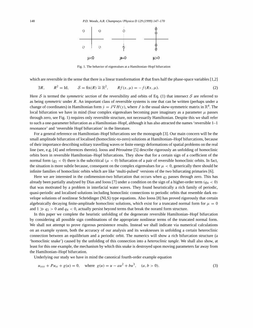
Fig. 1. The behavior of eigenvalues at a Hamiltonian–Hopf bifurcation

which are reversible in the sense that there is a linear transformationR that fixes half the phase-space variables [1,2]

∃R, R2 = Id, S = fix(R) ∼= R2, Rf (x, µ) = −f (Rx, µ). (2)

HereS is termed thesymmetric sectionof the reversibility and orbits of Eq. (1) that intersectS are referred toas beingsymmetricunderR. An important class of reversible systems is one that can be written (perhaps under achange of coordinates) in Hamiltonian formy = J∇H(y), whereJ is the usual skew-symmetric matrix inR4. Thelocal bifurcation we have in mind (four complex eigenvalues becoming pure imaginary as a parameterµ passesthrough zero, see Fig. 1) requires only reversible structure, not necessarily Hamiltonian. Despite this we shall referto such a one-parameter bifurcation as a Hamiltonian–Hopf, although it has also attracted the names ‘reversible 1–1resonance’ and ‘reversible Hopf bifurcation’ in the literature.

For a general reference on Hamiltonian–Hopf bifurcations see the monograph [3]. Our main concern will be thesmall amplitude bifurcation of localised (homoclinic-to-zero) solutions at Hamiltonian–Hopf bifurcations, becauseof their importance describing solitary travelling waves or finite energy deformations of spatial problems on the realline (see, e.g. [4] and references therein). Iooss and Pérouème [5] describe rigorously an unfolding of homoclinicorbits born in reversible Hamiltonian–Hopf bifurcations. They show that for a certain sign of a coefficient of thenormal form(q2 < 0) there is the subcritical(µ < 0) bifurcation of a pair of reversible homoclinic orbits. In fact,the situation is more subtle because, consequent on the complex eigenvalues forµ < 0, generically there should beinfinite families of homoclinic orbits which are like ‘multi-pulsed’ versions of the two bifurcating primaries [6].

Here we are interested in the codimension-two bifurcation that occurs whenq2 passes through zero. This hasalready been partially analysed by Dias and Iooss [7] under a condition on the sign of a higher-order term(q4 < 0)

that was motivated by a problem in interfacial water waves. They found heuristically a rich family of periodic,quasi-periodic and localised solutions including homoclinic connections to periodic orbits that resemble dark en-velope solutions of nonlinear Schrödinger (NLS) type equations. Also Iooss [8] has proved rigorously that certainalgebraically decaying finite-amplitude homoclinic solutions, which exist for a truncated normal form forµ = 0and 1� q2 > 0 andq4 < 0, actually persist beyond terms that break the noraml form structure.

In this paper we complete the heuristic unfolding of the degenerate reversible Hamiltonian–Hopf bifurcationby considering all possible sign combinations of the appropriate nonlinear terms of the truncated normal form.We shall not attempt to prove rigorous persistence results. Instead we shall indicate via numerical calculationson an example system, both the accuracy of our analysis and its weaknesses in unfolding a certain heteroclinicconnection between an equilibrium and a periodic orbit. The numerics will show a rich bifurcation structure (a‘homoclinic snake’) caused by the unfolding of this connection into aheteroclinic tangle. We shall also show, atleast for this one example, the mechanism by which this snake is destroyed upon moving parameters far away fromthe Hamiltonian–Hopf bifurcation.

Underlying our study we have in mind the canonical fourth-order example equation

utttt + Putt + g(u) = 0, where g(u) = u − au2 + bu3, (a, b > 0). (3)

P.D. Woods, A.R. Champneys / Physica D 129 (1999) 147–170 149

Under the change of coordinates, e.g.

q1 = u, q2 = utt + P + 2

2u, p1 = P − 2

2ut + uttt , p2 = ut ,

Eq. (3) is equivalent to a two-degree-of-freedom Hamiltonian dynamical system with energy

H = ututtt + P

2u2

t − 12u2

t t + G(u), where G(u) =∫ u

0g(v)dv. (4)

This dynamical system is also reversible in the sense of Eq. (2); specifically Eq. (3) is invariant under

R : (ut , uttt ) → (−ut , −uttt ) and t → −t. (5)

Finally, note that equilibria are given by

u = 0, or (if b > a/4) 1 − au + bu2 = 0. (6)

In Section 6 we shall show that this system undergoes a degenerate Hamiltonian–Hopf bifurcation at the originfor P = 2 andb = 38a/27, whereupon it satisfiesq4 > 0, the opposite case to that analysed by Dias and Iooss [7].

Eq. (3) arises in several contexts. Firstly [9–11], it represents the dimensionless equilibrium equation of an elasticstrut of deflectionu with respect to an infinite spatial coordinatet running along its length. HereP is the strengthof a compressive load andg(u) models the effect of a foundation with destiffening and re-stiffening nonlinearities.In that case, for long struts, the solutions of interest are homoclinic to zero, i.e.u(t) → 0 ast → ±∞. A secondscaling of Eq. (3) arises as the steady-state equation for the generalised Swift–Hohenberg equation [12,13] wherethere is interest in phase transitions modelled by homoclinic and heteroclinic connections among the origin and thenontrivial equilibria (6).

See [4] for a review of other applications of Eq. (3) for variousg(u), including (withg = u2) its derivation as arigorous centre-manifold reduction for capillary-gravity water waves with near-critical Bond and Froude numbers[14,15]. The behaviour of homoclinic solutions to Eq. (3) whenb = 0 is now almost completely understood[4,16,17]. Here we shall focus on the extra features that occur forb > 0.

The rest of the paper is outlined as follows. In Section 2, we shall recall the truncated normal form of theHamiltonian–Hopf bifurcation and its reduction [5] to a second-order nonlinear oscillator. Sections 3 and 4 thenanalyse solutions to this oscillator equation by examining carefully graphs of its potential energy. Particular attentionis paid to the existence of homoclinic and heteroclinic trajectories. Section 5 discusses questions of persistence ofsolutions with the addition of terms that break the completely integral normal form structure. Section 6 then presentsthe results of numerical experiments on Eq. (3). Finally, Section 7 draws conclusions, suggests future analyses andhighlights possible implications of the results for localised buckling and pattern formation problems.

2. Normal form

The Hamiltonian–Hopf bifurcation of a symmetric equilibrium of a reversible system occurs when two symmetricpairs of complex conjugate eigenvalues of the linearisation coalesce and form two pairs of imaginary eigenvaluesas shown in Fig. 1. Hereµ is the parameter that unfolds the bifurcation.

The normal form for the Hamiltonian–Hopf bifurcation is [5,7,18]

dA

dt= iωA + B + iAP

(µ; |A|2, i

2(AB − AB)

)+ RA, (7)


dB

dt= iωB + iBP

(µ; |A|2, i

2(AB − AB)

)+ AQ

(µ; |A|2, i

2(AB − AB)

)+ RB, (8)

whereP andQ are polynomials with real coefficients which to lowest order take the form

P(µ; x, y) = p1µ + p2x + p3y, Q(µ; x, y) = −q1µ + q2x + q3y + q4x2, (9)

andRA andRB are terms of higher order. In what follows the coefficients ofP are unimportant andq3 plays asubservient role. We assume that the bifurcation occurs in the way illustrated in Fig. 1, consequentially we maytakeq1 > 0. Following Iooss and Pérouème [5] we shall refer to the bifurcation on varyingµ as being sub- orsupercritical depending on whetherq2 < 0 orq2 > 0, respectively.

Generically it is unnecessary to includeq4 in an analysis of the bifurcation [5], unlessq2 is small [7] whichis precisely the situation that interests us. Therefore, we shall regardµ andq2 as independent small parametersunfolding the codimension-two point where they are both zero. A scaling argument in [7] shows that if

q2 = ε, and A = O(√

ε), B = O(ε√

ε), t = O(√

ε), µ = O(ε2),

then the ignored terms in the normal form upon takingRA = RB = 0 and Eq. (9) are consistently of higher orderin ε. Therefore, at least formally, to lowest order inε the assumed forms ofP andQ are sufficient to unfold thecodimension-two bifurcation.

The system (7) and (8) withRA = RB = 0 is completely integrable with integralsK andH defined by

K(µ, A, B) = i

2(AB − AB),

H

(µ, |A|2, |B|2, i

2K

)= |B|2 −

∫ |A|2

0Q(µ, s, K)ds.

Using these integrals it is straightforward to write the system as a single nonlinear oscillator equation forx = |A|2.Note that choosing such a coordinate in effect factors out the fast dynamics which are terms inA proportional toeiω. Specifically, from Eq. (7) without remainder terms we have dx/dt = AB + BA, and hence

(dx

dt

)2

= 4x

(H +

∫ x

0Q(µ, s, K)ds

)− 4K2 := 4f (x). (10)

This equation may be viewed as the expression for conservation of zero total energy of a particle of unit mass andpositionx confined to lie in a potential well, with potential−4f (x). Taking the approximations (9), the functionf

is of the form

f (x : µ, H, K) = 13q4x

4 + 12q2x

3 + (q3K − q1µ)x2 + Hx − K2. (11)

To understand the dynamics near the codimension-two point we shall study the roots of the negative of thepotentialf (x) for µ andq2 small.

Equivalently, upon differentiating with respect tot , Eq. (10) can be expressed as a nonlinear oscillator equationfor xtt in terms ofx. Then, from the given form off , one could attempt to read off explicit solutions at certainparameter values (such as homoclinic orbits in terms of hyperbolic secant funcitons). Rather than adopting such ananalytic approach, we shall rely on a geometric approach, since the shape off entirely determines the dynamics ofEq. (10).

Now, sincex is real, solutions to Eq. (10) only make sense iff ≥ 0. Also, sincex = |A|2, we are only interestedin solutions forx > 0. Our primary concern will be with homoclinic orbits, these are represented by a particle


which starts at rest at a double rootx∗ of f (corresponding to an equilibrium of Eq. (10)) and then passes upwardsuntil another root is encountered at which point it must return backwards along with the same path. Thus, for orbitshomoclinic to an equilibriumx = x∗, there are conditions on the shape off (x)

• f (x) must become positive on one side ofx = x∗ (sox∗ cannot be a local maximum off ); also if x∗ is theorigin, then we must havef (x) > 0 for all x < a for somea > 0.

• If f (x) locally increases for one sign ofx − x∗, then for a homoclinic orbit to exist there must be a nonnegativeroot bounding this region of positivef .We should stress the relation between homoclinic orbits of the reduced oscillator (10) and truncated normal forms

(7) and (8) withRA = RB = 0 andP andQ given by Eq. (9). Eq. (10) is the equation for the square amplitude ofA. Similar equations can easily be derived for the phase ofA and the amplitude and phase ofB ([5], Eq. (9)). Theleading order terms of these three equations just give rotation corresponding to the imaginary eigenvalues±iω. Allother terms are slaved to Eq. (10) in that the right-hand sides depend only onµ, x = |A|2 and the integralsH andK. The form of these equations implies that solutions to Eq. (10) correspond to a one-parameter family of solutionsof the full system parametrised by shifts in phase(A, B) → (Aeiφ, Beiφ). Also, nontrivial equilibria of Eq. (10)correspond to periodic orbits of the normal form. Hence a homoclinic orbit to the origin of the amplitude equation(10) corresponds to a one-parameter family of homoclinic solutions to the origin of Eqs. (7) and (8), whereas ahomoclinic orbit to a nontrivial equilibrium corresponds to a one-parameter family of homoclinic connections to aperiodic orbit in the normal form equations.

It is a much more delicate question to determine persistence of solutions under the inclusion of higher-ordertermsRA, RB 6= 0 which break the completely integrable structure of the normal form. We shall return to thisquestion in Section 5 below. In the meantime we note that the origin(A, B) = (0, 0) satisfiesH = K = 0 sohomoclinic solutions to the origin, ‘bright solitons’ in the parlance of NLS-type equations, must lie in these zeroenergy surfaces. We treat this special case first in Section 3 that follows. After that we treat general values ofH andK and look for possible homoclinic connections to nontrivial equilibria. Such homoclinic connections to periodicorbits have been given the name ‘dark solitons’ (see, e.g. [7]). We shall refer tobright homoclinic solutions as thosewhosex-value at their mid-point is higher than thex-value to which they asymptote anddarkhomoclinic solutionsas those obeying the revese.

3. Homoclinic orbits in the zero energy surface

We start our analysis by considering Eq. (11) withH = K = 0,(

dx

dt

)2

= 4f (x), where f (x) = q4

3x4 + q2

2x3 − q1µx2. (12)

The dynamics of Eq. (12) and hence the existence or otherwise of homoclinic orbits is crucially dependent on thesign ofq4. The two cases are treated separately.

3.1. q4 positive

First, dividing out the double root off at the origin leaves a quadratic inx

g(x) = q4

3x2 + q2

2x − q1µ,


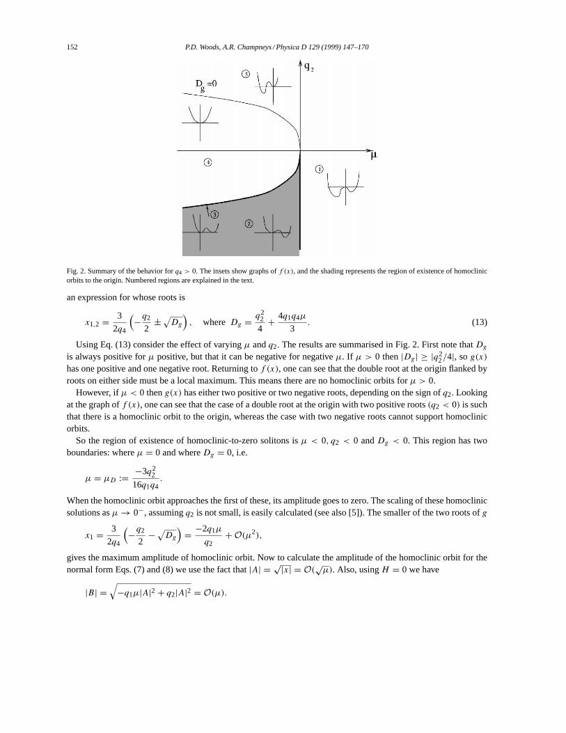
Fig. 2. Summary of the behavior forq4 > 0. The insets show graphs off (x), and the shading represents the region of existence of homoclinicorbits to the origin. Numbered regions are explained in the text.

an expression for whose roots is

x1,2 = 3

2q4

(−q2

2± √

Dg

), where Dg = q2

2

4+ 4q1q4µ

3. (13)

Using Eq. (13) consider the effect of varyingµ andq2. The results are summarised in Fig. 2. First note thatDg

is always positive forµ positive, but that it can be negative for negativeµ. If µ > 0 then|Dg| ≥ |q22/4|, sog(x)

has one positive and one negative root. Returning tof (x), one can see that the double root at the origin flanked byroots on either side must be a local maximum. This means there are no homoclinic orbits forµ > 0.

However, ifµ < 0 theng(x) has either two positive or two negative roots, depending on the sign ofq2. Lookingat the graph off (x), one can see that the case of a double root at the origin with two positive roots(q2 < 0) is suchthat there is a homoclinic orbit to the origin, whereas the case with two negative roots cannot support homoclinicorbits.

So the region of existence of homoclinic-to-zero solitons isµ < 0, q2 < 0 andDg < 0. This region has twoboundaries: whereµ = 0 and whereDg = 0, i.e.

µ = µD := −3q22

16q1q4.

When the homoclinic orbit approaches the first of these, its amplitude goes to zero. The scaling of these homoclinicsolutions asµ → 0−, assumingq2 is not small, is easily calculated (see also [5]). The smaller of the two roots ofg

x1 = 3

2q4

(−q2

2− √

Dg

)= −2q1µ

q2+O(µ2),

gives the maximum amplitude of homoclinic orbit. Now to calculate the amplitude of the homoclinic orbit for thenormal form Eqs. (7) and (8) we use the fact that|A| = √|x| = O(

√µ). Also, usingH = 0 we have

|B| =√

−q1µ|A|2 + q2|A|2 = O(µ).


So the one-parameter family of homoclinic solutions looks like

A(t) = O(√

µ)exp(iωt + φ), B(t) = O(µ)exp(iωt + φ), (14)

for arbitrary initial phases 0≤ φ < 2π .At the other boundary of the region of existence of homoclinic solutions there is a double root ofg at x =

−3q2/4q4, which corresponds in the full normal form (7) and (8) to a finite-amplitude periodic orbit. Hence thehomoclinic orbit to the origin has become a heteroclinic connection between the origin and this periodic orbit. Theexistence of this heteroclinic orbit will play a crucial role in the numerical experiments in Section 6. (Note that theother branch of the curveDg = 0 has no meaning since the double root occurs forx < 0.)

Thus, there are four open parameter regions in the(µ, q2) plane corresponding to qualitatively distinct dynamics,as shown in Fig. 2. The region numbers in the figure are the same as in the summary below.1. Whenµ > 0 the graph off (x) has a negative root, a double root at the origin and a positive root. The fact

that the double root is a maximum precludes the existence of homoclinic orbits of Eq. (10) sincef is negativelocally.

2. When 0> µ > µD andq2 < 0, thenf (x) has a double root at the origin and two positive roots. Since thedouble root is a local minimum, there are homoclinic orbits, the maximum amplitude of which are given by thefirst positive root.

3. Whenµ = µD andq2 < 0 there is a double root atx = 0 and also atx = −3q2/4q4. This means that on thishalf-parabola there is a heteroclinic connection (see above).

4. Whenµ < µD there are no zeros off other than the double root at the origin.5. When 0> µ > µD andq2 > 0, the two nontrivial roots off (x) are negative and so there can be no homoclinic

orbits forx > 0.We have focussed on the possible existence of homoclinic solutions, but from the shapes of the graphs off

illustrated in the insets to Fig. 2, the reader may also infer information about periodic and quasi-periodic solutionswith H = K = 0.

3.2. q4 negative

This case has been analysed in [7,8]. For completeness, we list here the results which may be obtained usingthe same methods as the previous subsection. The numbered sections below refer to the numerically labeled openparameter regions and special curves numbered in Fig. 3.1. On the lineµ0, q2 > 0 there is a triple root at the origin and a positive root withf positive inbetween. Such

a graph represents a homoclinic orbit to a degenerate equilibrium at the origin. We note that such a solutiondecays algebraically to zero (for more details see [8])

2. In the regionµ < 0 in addition to a local minimum off at the origin, there is a positive and a negative root.Hence there is a homoclinic orbit. Note that, in contrast to the case whereq4 > 0 there are homoclinic orbitsto the origin for both subcritical(q2 < 0) andsupercritical(q2 > 0) bifurcations. The distinction between thetwo cases, is that on decreasingµ from zero, the homoclinic orbits bifurcate from small amplitude forq2 < 0,but from finite-amplitude algebraically decaying solutions whenq2 > 0. In particular, forq2 < 0 the scalings(14) hold, whereas forq2 > 0, the amplitude of the homoclinic is finite atµ = 0. At the transition betweensuper- and subcritically,q2 = 0 we have

A(t) = O(4√

µ)exp(iωt + φ), B(t) = O(µ3/4)exp(iωt + φ). (15)

3. On the lineµ = 0, q2 < 0 there is a triple root at the origin and a negative root. There are no homoclinic orbits.


Fig. 3. Analogous to Fig. 2 but forq4 < 0.

4. In the region 0< µ < µD, q2 < 0 there is a double root at the origin and two negative roots.5. In the region 0< µD < µ there is only the double root at the origin.6. In the region 0< µ < µD, q2 > 0 there is a minimum at the origin and two positive roots. Hence there are no

homoclinic orbits.In summary, there are exponentially decaying homoclinic orbits for allµ < 0 and algebraically decaying homoclinicorbits forµ = 0, q2 > 0.

4. Homoclinic orbits in nonzero energy surfaces

Dias and Iooss [7] showed the existence of various kinds of homoclinic-to-periodic solutions of Eq. (10) for(H, K) 6= (0, 0) in the caseq2 > 0, q4 < 0. We shall repeat their analysis techniques and extend it to cover allpossible combinations of signs ofq2 andq4. We shall also consider the special case that arises whenq3 is taken tobe zero.

As the normal form motivates this investigation, onlyx > 0 andf (x) > 0 are considered. We start by lookingat conditions for multiple roots off , which in general represent periodic solutions of Eqs. (7) and (8) and mayrepresent the end points of homoclinic solutions.

4.1. Conditions for multiple roots off

For double roots we require

f (x; H, K, µ) = 13q4x

4 + 12q2x

3 − (q1µ − q3K)x2 + Hx − K2 = 0, (16)

df

dx(x; H, K, µ) = 4

3q4x3 + 3

2q2x2 − 2(q1µ − q3K)x + H = 0. (17)

One can eliminateH between these equations, which gives a quadratic

K2 + q3x2K + q4x

4 + q2x3 − q1µx2 = 0, (18)


that can be solved forK if its discriminant1 is positive

1 = x2((q23 − 4q4)x

2 − 4q2x + 4q1µ) ≥ 0. (19)

We denote byµm the value ofµ that makes the discriminant of the nontrivial quadratic factor of Eq. (19) vanish,its value is

µm = q22

q1(q23 − 4q4)

, xm = 2q2

q23 − 4q4

. (20)

For µ > µm, 1 is positive for all values ofx. Hence, for each value ofx there are two values ofK (andconsequentlyH ) solving Eqs. (16) and (17),

K± = 12(−q3x

2 ±√

1), H± = −43q4x

3 − 32q4x

2 + 2(q1µ − q3K±)x.

Note thatK+ is zero when−4q4x2 − 4q2x + 4q1 = 0, whereas,K− is never zero except atx = 0.

The boundary in the(x, µ) plane of existence of double roots of Eq. (18) is given by1 = 0, i.e.

D =(x, µ) : x = x± :=

2q2 ± 2√

−q22 − q1µ(q2

3 − 4q4)

q23 − 4q4

. (21)

OnD, there is only oneK-value giving a solution.We now look for triple roots. They can be obtained by settingf (x) and its first two derivatives equal to zero.

This leads to the following expressions:

K±t = ±√

q4x4 + 12q2x3, H±t = 8

3q4x3 + 3

2q2x2, (22)

q1µ±t = ±q3

√q4x4 + 1

2q2x3 + 2q4x2 + 3

2q2x. (23)

These conditions define a curveT of triple roots in the(x, µ) plane. Setting the third derivative equal to zero alsogives an expression for quadruple roots, namely that in addition to Eqs. (22) and (23) we have

x = xq := −3q2

8q4.

So quadruple roots occur at isolated pointsQ in the(x, u) plane, which, sincex must be positive in Eq. (10), areonly meaningful whenq4 andq2 have opposite signs.

In what follows we shall view regions in the(x, µ) plane corresponding to differing numbers of multiple rootsupon varyingK. We shall also infer information on the existence of homoclinic orbits from the location of theseroots inx, and from the shape of the graph off (x; H, K, µ). As in Section 3, we leave it to the reader to gleaninformation from the various graphs about existence of periodic and quasi-periodic solutions.

4.2. q4 negative

4.2.1. Supercritical bifurcation:q2 > 0If we setq4 < 0 andq2 > 0 in Eq. (21) thenD has a maximum with respect toµ at

M : (xm, µm) =(

4

5,

4

5

). (24)

So forµ > µm there are two surfaces of solutions to Eq. (18) for each value ofµ; while for 0 < µ < µm there arefour, two each side ofD. See Fig. 4. AlongD, K+ andK− merge smoothly in a fold. Hence, atxm all four solution


Fig. 4. Curves of solutions to Eq. (18) in the(x, K) plane for (a)µ = 2 > µm = 4/5, (b)µ = 1/2 < µm, (c) µ = 0 < µm for q4 < 0, q2 > 0(q4 = −1, q3 = 1, q2 = 2, q1 = 1).

Fig. 5. The(x, K) and(µ, K) planes forµ = µm = 4/5 andx = xm = 4/5 for q4 < 0, q2 > 0 (q4 = −1, q3 = 1, q2 = 2, q1 = 1).

surfaces are pinched together; see Fig. 5. Forµ < 0 there are only two sets of solutions (forx > x+) becausex−

becomes negative. Sheets of solutions join atD.There are also triple roots, given by puttingq4 < 0, q2 > 0 in Eqs. (22) and (23). On this curve,T , there are two

K-values,K+t andK−t with correspondingµ-valuesµ+t andµ−t . T is a closed curve because the square-rootedquantity in Eqs. (22) and (23) is undefined forx > q2/2q4.


Fig. 6. Projections of degenerate curves and points onto the(x, µ) plane forq4 < 0, q2 > 0. See text for details.

Fig. 7. Creating homoclinic orbits by varyingµ. Depicted are graphs off (x), the bold portions of which correspond to homoclinic orbits.

Fig. 6 shows the curvesD, T + andT −, and pointsQ andM projected onto the(x, µ) plane. In this and subsequentsimilar figures, numbers in circles attached to regions, curves or points refer to the number of homoclinic orbitsthat occur (possibly in different sheets in the(K, x) plane) at those(x, µ)-values. By thex-value of a homoclinicorbit we mean the value ofx at the equilibrium or periodic orbit (double root off ) that the solution is asymptoticto. Some representative graphs of thef (x) are also given as inserts in the figure.

We now know about what types of double roots off there are forq4 < 0, q2 > 0: double roots everywhereoutside the region bounded by the curveD of the discriminant begin zero, and isolated curves of triple roots. Nowwe try to locate all possible homoclinic solutions. First note that there are two ways homoclinic orbits can be createdas the parameterµ is varied (see Fig. 7). One notes that the first method involves a positivey-intercept off , this isprohibited by the form of Eq. (16). So there have to be triple roots for there to be the creation of homoclinic orbits.Thus, it is important to note from the figures howT interacts withK+ andK−.

In K+, f (x) admits a pair of homoclinic orbits in the region in Fig. 6 bounded byT + andD. Similarly, inK−, f (x) admits a pair of homoclinic orbits in the region of Fig. 6 bounded byT − andD. At T ± in both cases,there are algebraically decaying bright homoclinic orbits except in the region ofT between the two quadruple rootpointsQ. In this latter regionT represents algebraically decaying dark homoclinic orbits. Fig. 5 shows the processby whichT changesK-sheets atM.

4.2.2. Subcritical bifurcation:q2 < 0If q2 < 0 while q4 < 0 in Eq. (21), then the boundaryD(1 = 0), of double roots has a maximum inµ at

(xm, µm) = (−4/5, 4/5) wherexm andµm are given by Eq. (24). A typical(x, K) projection looks like graph Fig.4(c). The boundaryD goes through the origin in the(x±, µ) plane, see Fig. 8.T consists of one point, the origin(a negative triple root).


Fig. 8. Projections of degenerate curves and points onto the(x, µ) plane forq4 < 0, q2 < 0. See text for details.

4.3. q4 positive

Now we move on to the case not analyzed by Dias and Iooss [7], but which has relevance to the example (3). Ifq4 > 0, then the sign of 4q4 − q2

3 is important. So, taking either sign ofq2, there are four subcases.

4.3.1. 4q4 > q23, supercritical

If 4q4 > q23 andq2 > 0 thenD(1 = 0) has a minimum inµ at zero. Double roots exist for 0< x < x+. D

is a parabola that points up rather than down in the(x, µ) plane (as was the case forq4 < 0) and passes throughthe origin. There are two sheets of double rootsK±. A typical graph of solutions in the(x, K) plane would looklike Fig. 11(a) (even though that was computed forq2 < 0). T + lies in K+ andT − in K−. T is defined for allx > 0. The square-rooted quantity in Eqs. (22) and (23) has no positive roots, so thatT is unbounded in the(x, µ)

plane. Fig. 9(a) depicts the general situation. Note that the curve of triple roots no longer represents algebraicallydecaying homoclinic orbits whenq4 > 0, because of the shape of the associated potential. The root other than thetriple root is negative and so is not important in the normal form. However,T retains its importance in the creationof homoclinic orbits.

Homoclinic orbits are found in the same way as in theq4 < 0 supercritical case. InK+ there is a single doubleroot between theµ-axis andT +. CrossingT causesf to admit a dark homoclinic orbit. This persists untilD atx+, where the two sheets join. Similarly, inK− there is a single double root untilT − is reached. BeyondT , f

represents a dark homoclinic orbit. This remains untilD is reached.

4.3.2. q23 > 4q4 > 0, supercritical

The boundaryD now points down instead of up (see Fig. 9(b)).D has a maximum at(xm, µm) = (4/5, 4/5).Fig. 10 illustrates anx − K section for constantµ = 0.5, where one sees thatT + lies in K+ and thatT − lies inK− and then inK+. f (x) represents homoclinic orbits inK+ betweenT + andD and also in the regionx > D

andx > T −.In K−, f (x) represents homoclinic orbits in the region bounded by the origin,T −, x = 2q2/(q

23 − 4q4)

andD.

4.3.3. 4q4 > q23, subcritical

The boundary of double rootsD(1 = 0) has a minimum at(xm, µm) = (4/3, −4/3). Double roots exist for0 < x− < x < x+. D is a parabola that points up rather than down. The boundary passes through the origin. There


Fig. 9. Projections of degenerate curves and points onto the(x, µ) plane forq4 > 0, q2 > 0 and (a)q23 < 4q4, (b)q2

3 > 4q4. See text for details.

Fig. 10. Solutions to Eq. (18) in the(x, K) plane forµ = 1/2, q4 > 0, q2 > 0 andq23 > 4q4. See text for details.

are two sheets of double rootsK±. The two sheets join onD. Triple roots can exist. See Fig. 12(a) for the picture.The square rooted quantity in Eqs. (22) and (23) is defined forx = 0 and forx > q2/2q4. There are no quadrupleroots becausex = −3q2/8q4 falls outside the range for whichµ is defined.

Fig. 11 shows thatT + lies in K+ and thatT − lies in K−. T changes sheets when it touchesD at (xm, µm).We know that to the left toT + in K+ there are simple double roots. CrossingT in K+ causesf to represent


Fig. 11. Solutions to Eq. (18) in the(x, K) plane for (a)µ = 1, (b)µ = 1/2, (c)µ = −1 for q4 > 0, q2 < 0 and 4q4 > q23.

dark homoclinic orbits. InK−, f represents simple double roots untilx crossesT −. OnD, f (x−) represents localmaxima andf (x+) represents dark homoclinic orbits. The change occurs atxm.

4.3.4. q23 > 4q4 > 0, subcritical

As we saw in the corresponding supercritical caseD points down instead of up. As a resultD has no turningpoint forx > 0 and so it does not touchT , see Fig 12(b). SoT lies in whollyK+ andf (x) represents homoclinicorbits only inK+ bounded byT .

4.4. Degenerate caseq3 = 0

There is one kind of special case,q3 = 0, that affects all the cases analysed above. The degeneracy causesK+2 = K−2 andH+ = H−, so there are two sheets of identical solutions. AlsoK± = 0 on D(1 = 0). Theprincipal differences fromq3 6= 0 in the various cases are as follows:1. Forq4 < 0, q2 > 0, T now forms one branch, withf (x) representing double roots outside and homoclinic

orbits betweenT andD. (See [7] figure 5.2 for the effects of varyingq3.)2. If q4 > 0, q2 > 0, T now forms a single branch withf (x) having double roots between theµ-axis andT and

having homoclinic orbits betweenT andD.3. Forq4 > 0, q2 < 0, T forms a single branch withf (x) representing double roots between theµ-axis andT .

It represents homoclinic orbits betweenT andD(x+).


Fig. 12. Projection of degenerate curves and points onto the(x, µ) plane forq4 > 0, q2 < 0 and (a)q23 < 4q4, (b)q2

3 > 4q4. See text for details.

4.5. Summary

We have shown that there are two sheets of solutions of double roots off (x) in the(x, µ) plane and that tripleroots off (x) lie on a curve in these sheets. Let us summarise the conditions for these curves to posses homoclinicconnections.• q4 < 0, q2 > 0: a bounded curve of triple roots lies in both sheets of solutions. It together with the boundary of

existence of solutions(1 = 0) enclose regions of homoclinic orbits. The quadratic curve of1 = 0 points down.• q4 < 0, q2 < 0, there are no triple roots and no homoclinic orbits. The quadratic curve of1 = 0 points down.• 4q4 − q2

3 > 0, q2 of either sign, there are unbounded curves of triple roots in both sheets, which together withthe boundary enclose regions of dark homoclinic orbits. The triple roots do not represent homoclinic orbits. Thequadratic curve of1 = 0 points up.

• q4 > 0, q23 > 4q4, q2 > 0, there is an unbounded curve of triple roots inK+ and a small section of triple roots

in K−. So there are homoclinic orbits in both surfaces.• q4 > 0, q2

3 > 4q4 > 0, there is an unbounded curve of triple roots inK+ only, so there are homoclinic orbits inK+ only.


5. Persistence of solutions and heteroclinic tangles

So far we have considered only solutions of the normal form Eqs. (7) and (8) withRA = RB = 0. The question ofpersistence of solutions under the addition of remainder terms that break the integrable structure of the normal formcompletely is more delicate. We shall only consider this question for solutions (either homoclinic or heteroclinic)that lie in the unstable manifold of the originWu(0) for µ < 0. Then, since the origin is a saddle-focus,Wu(0) istwo-dimensional and transverse intersections betweenWu(0) and the symmetric sectionS will survive under smallperturbations. Such solutions will be symmetric homoclinic orbits.

Now, for subcritical bifurcations away from the codimension-two point, i.e. whenq2 < 0 is not small, we have thebifurcation forµ < 0 of a one-parameter family Eq. (14) of homoclinic orbits of the truncated normal form Eqs. (7)and (8). A careful argument in [5] shows that when remainder terms are included that break the integrable structureof the normal form completely, the two solutions with phasesφ = 0 andπ correspond to symmetric solutions andthey do indeed persist forµ sufficiently small. In fact, if we can prove that these two orbits are transverse, thenthe analysis of Härterich [6] for reversible systems or Devaney [19] for Hamiltonian systems will additionally giveinfinitely manyN -pulse orbits (homoclinic solutions which resembleN copies of the primary placed end to end)for eachN and each smallµ, although none of them bifurcates fromµ = 0. Indeed, an intricate bifurcation pictureof multi-pulse solutions has been found both numerically [16] and asymptotically [20] for Eq. (3) withb = 0.

Also, for µ = 0 Iooss [8] has shown the persistence of the two symmetric algebraically decaying solitary waves(limits of Eq. (15) asµ → 0, see Fig. 3) forq4 < 0 andq2 > 0 small.

We now turn our attention to the heteroclinic connections that occur along the curveµ = µD for q4 > 0 andq2 < 0 (see Fig. 2). Recall that these correspond to heteroclinic connections from the origin to the small-amplitudeperiodic solution represented by the nontrivial double root off (|A|2). Putting back in the arbitrary phaseφ, wehave a one-parameter family of such heteroclinic connections. When normal-form breaking remainder terms areadded, such a family of heteroclinic connections is structurally unstable because it involves the identification oftwo-dimensional stable and unstable manifolds of the origin and the periodic orbit. A Melnikov-type analysis wouldneed to be performed in order to judge how this highly degenerate situation unfolds upon addition of remaindertermsRA andRB . Such an analysis is likely to be highly involved and be sensitively dependent on the form ofthe remainders, and we do not attempt to perform it here. Instead we merely state that one of the simplest genericunfoldings is that the degenerate heteroclinic family breaks up into a pair of heteroclinic tangencies occurring atnearbyµ-values.

Fig. 13 shows how such a bifurcation sequence would unfold for reversible Hamiltonian systems. The dynamicsare clearly highly complex, but we remark only how the unfolding leads to infinitely many symmetric homoclinicorbits (intersections betweenWu(0) and the symmetric sectionS). Each successive homoclinic solution has onemore oscillation near the periodic orbitL. Carefully tracing how the infinitely many homoclinic orbits in panel (d)of Fig. 13 are created as the parameter varies, we find that all the solutions lie on a single curve in a bifurcationdiagram. This curve snakes to and fro, involving successive folds as the solution generates more and more bumps(oscillations close to the periodic orbit). See Fig. 14 below for a numerically computed curve and ([21], Section 4)for a more detailed justification of the construction in Fig. 13 and why it leads to such a snaking curve. Finally, sincethere are two primary solutions which bifurcate fromµ = 0, we should expect to see this snaking curve repeatedfor each of the two primaries (see Fig. 16 below).

Let us reiterate that we have not proved anything, we have merely constructed a simple possible unfolding of thedegenerate heteroclinic connection in the normal form. As we shall now see though, this unfolding is borne out innumerical experiments on the example equation (3).


Fig. 13. Illustrating the parameter unfolding of two successive heteroclinic tangencies between a saddle-focus equilibriumO and a saddle-typeperiodic orbitL for a four-dimensional reversible Hamiltonian system. The picture is drawn schematically by taking a formal Poincare sectionwithin the zero level set of the Hamiltonian function,S is the symmetric section, and unstable and stable manifolds are depicted by solid andbroken lines, respectively. Each point at whichWu(0) intersectsS corresponds to a symmetric homoclinic orbit. For the unfolding of the normalform, panels (a)–(f) correspond to increasingµ through the critical valueµD = −3q2

2/16q1q4 for q4 > 0 andq2 < 0.

Fig. 14. Continuation inP of the primary homoclinic orbit from the reversible Hopf bifuration atP = 2 of Eq. (3) withb = 0.29.

6. Numerical results

With the aid of Maple program derived from ([22], Ex.15, Section 8.7) we have calculated the important normalform coefficients for Eq. (3) (see [23] for the details). Specifically we get

µ = P − 2, (25)

q1 = 1

4, (26)


Fig. 15. Continuation inP for b = 0.3 showing the formation of multi-pulse solutions for both the primary and the2(2) branch.

q2 = −19

18a2 + 3

4b, (27)

q4 = 12007

576a2b − 687295

46656a4 − 327

512b2. (28)

Soq2 changes sign atb = 38a2/27 and at this valueq4 is positive.

6.1. Homoclinic snaking

In what follows we shall compute bifurcation curvers of homoclinic and heteroclinic orbits to Eq. (3) asP andb

vary, holdinga fixed at 1. Note that, provided it is nonzero,a can be scaled out of the equation by the transformationu = au hence there is no los of generality. All computations are performed using the numerical continuation softwareauto [24]. Fig. 14 shows the bifurcation diagram, for the typical valueb = 0.29 (but note this is a long way from38/27 whereq2 = 0), of the simplest symmetric homoclinic orbit which emanates from the Hamiltonian–Hopfbifurcation point atP = 2. The ordinate of this and subsequent bifurcation diagrams is a constant multiple of thevectorL2-norm of(u(t), u′(t), u′′(t), u′′′(t)). At each successive pair of limit points of the curve, the homoclinicsolution gains an extra pair of ‘bumps’ close to the periodic solution. The insets in the figure show this processfor the first three folds. As the curve climbs inL2-norm the process repeats, creating a homoclinic solution witharbitrarily large norm and arbitrarily many large-amplitude bumps. From the figure it might appear that all the limitpoints appear to occur at only two values ofP (see also Figs. 15 and 16). However, in fact what we find is that thelimit points form two sequences that converge converge rapidly onto two distinctP -values. This corresponds to thetheory embodied in Fig. 13 in the case where the periodic orbitL has positive nontrivial Floquet multipliers (see


Fig. 16. Indicating how the width of the snaking decreases rapidly asb increases: (a)b = 0.3 and (b)b = 0.594.

Fig. 17. (a) The results of two-parameter continuation inP andb (plotted asq2 = −19/18+ (3/4)b) of an inner and outer limit point (withrespect toP ) of the primary homoclinic orbit. The dashed line corresponds to the kink solution forb = 2/9 (see Section 6.2). (b) A comparisonwith normal form theory near(P, q2) = (2, 0). The line represents the normal-form calculation of the heteroclinic connection using Eqs.(25)–(28). The points represent numerically calculated curves of limit points.

([21], Section 4) for a more detailed argument). The theory shows that the two sequences ofP -values of the limitpoints should converge to the two heteroclinic-tangency parameter values, moreover, this convergence should befrom the right in both cases.

Figs. 15 and 16 show similar figures for two differentb-values, one further away and one closer to the codimension-two pointb = 38/27. In both figures, we have also computed the other branch of homoclinic solutions that bifurcatesfromP = 2 (in the notation of [16] this is the2(2) branch). Note how the bifurcation branches of these two homoclinicorbits become intertwined. The primary creates solutions with odd numbers of bumps close to the periodic orbitand the2(2) creates homoclinic solutions with even numbers of bumps. Asb is decreased towards 38/27, the valueat whichq2 = 0 for Eq. (3), the oscillations inP decrease in amplitude (see Fig. 16).

Fig. 17 shows the distribution of limit points asµ andq2 are varied for Eq. (3). The two numerical curves oflimit points were taken on the primary branch after sufficiently many wiggles to be close to the twoµ-values atwhich the limit points converge (to heteroclinic tangencies). Note from Fig. 17(b) how the numerical and theoretical


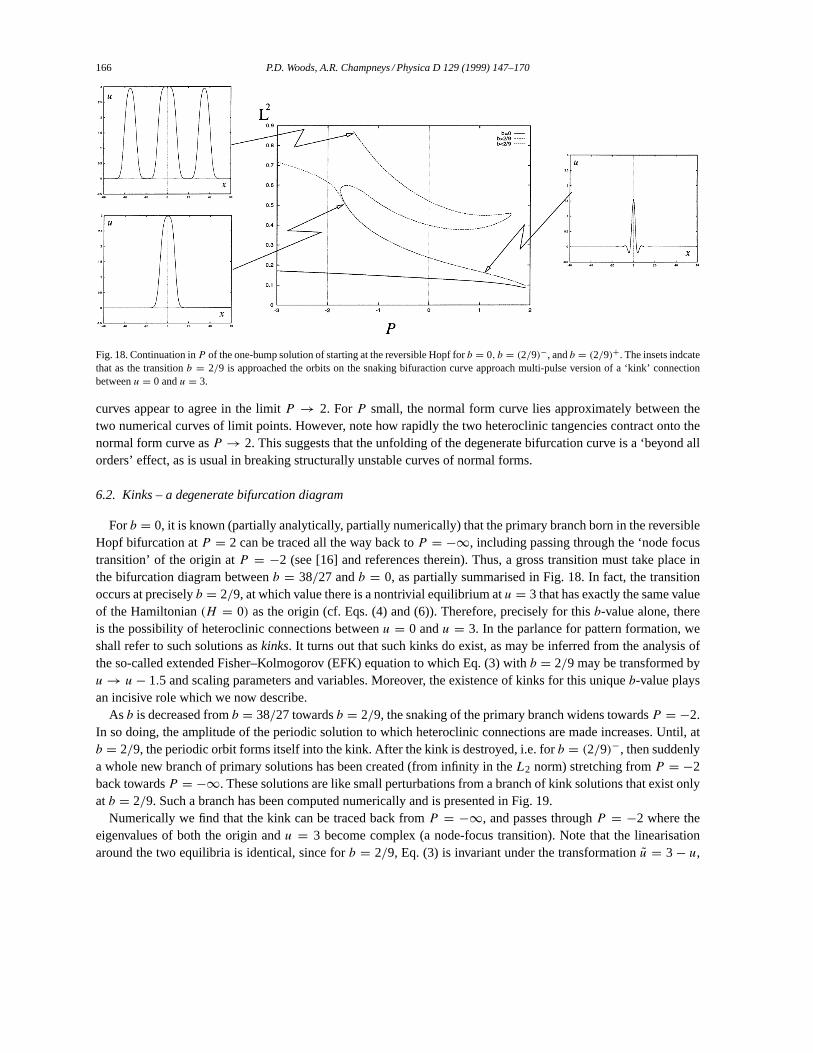
Fig. 18. Continuation inP of the one-bump solution of starting at the reversible Hopf forb = 0, b = (2/9)−, andb = (2/9)+. The insets indcatethat as the transitionb = 2/9 is approached the orbits on the snaking bifuraction curve approach multi-pulse version of a ‘kink’ connectionbetweenu = 0 andu = 3.

curves appear to agree in the limitP → 2. ForP small, the normal form curve lies approximately between thetwo numerical curves of limit points. However, note how rapidly the two heteroclinic tangencies contract onto thenormal form curve asP → 2. This suggests that the unfolding of the degenerate bifurcation curve is a ‘beyond allorders’ effect, as is usual in breaking structurally unstable curves of normal forms.

6.2. Kinks – a degenerate bifurcation diagram

Forb = 0, it is known (partially analytically, partially numerically) that the primary branch born in the reversibleHopf bifurcation atP = 2 can be traced all the way back toP = −∞, including passing through the ‘node focustransition’ of the origin atP = −2 (see [16] and references therein). Thus, a gross transition must take place inthe bifurcation diagram betweenb = 38/27 andb = 0, as partially summarised in Fig. 18. In fact, the transitionoccurs at preciselyb = 2/9, at which value there is a nontrivial equilibrium atu = 3 that has exactly the same valueof the Hamiltonian(H = 0) as the origin (cf. Eqs. (4) and (6)). Therefore, precisely for thisb-value alone, thereis the possibility of heteroclinic connections betweenu = 0 andu = 3. In the parlance for pattern formation, weshall refer to such solutions askinks. It turns out that such kinks do exist, as may be inferred from the analysis ofthe so-called extended Fisher–Kolmogorov (EFK) equation to which Eq. (3) withb = 2/9 may be transformed byu → u − 1.5 and scaling parameters and variables. Moreover, the existence of kinks for this uniqueb-value playsan incisive role which we now describe.

As b is decreased fromb = 38/27 towardsb = 2/9, the snaking of the primary branch widens towardsP = −2.In so doing, the amplitude of the periodic solution to which heteroclinic connections are made increases. Until, atb = 2/9, the periodic orbit forms itself into the kink. After the kink is destroyed, i.e. forb = (2/9)−, then suddenlya whole new branch of primary solutions has been created (from infinity in theL2 norm) stretching fromP = −2back towardsP = −∞. These solutions are like small perturbations from a branch of kink solutions that exist onlyatb = 2/9. Such a branch has been computed numerically and is presented in Fig. 19.

Numerically we find that the kink can be traced back fromP = −∞, and passes throughP = −2 where theeigenvalues of both the origin andu = 3 become complex (a node-focus transition). Note that the linearisationaround the two equilibria is identical, since forb = 2/9, Eq. (3) is invariant under the transformationu = 3 − u,


Fig. 19. Kink solutions forb = 2/9.

Fig. 20. Multi-kink solutions forb = 2/9.

which maps the two equilibria into one another. Moreover, owing to this symmetry all kinks computed in Fig. 19are odd inu − 1.5. Hence the kinks develop decaying oscillations in their tails as they pass throughP = −2.At P ≈ 1.645 the kink turns around at a limit point in its bifurcation diagram and returns towardsP = −2 asa three-transition kink solution. From theoretical considerations we strongly suspect that such a solution survivesback toP = −2 where the six layers of near constantu = 0 oru = 3 become infinitely wide. However, there arenumerical difficulties in computing towards this limitingP -value.

Finally, we note that the kink solutions in Fig. 19 are only two of an infinite family that appear to exist forall P ∈ (−2, 2) whenb = 2/9. Figs. 20 and 21 show a bifurcation diagram of a sample of extra multi-layeredkinks. Again, for theoretical reasons we expect that other than the primary kink solution, all others terminate at thenode-focus transitionP = −2 by the transition layers becoming infinitely wide asP → −2.


Fig. 21. Other complex kink solutions forb = 2/9.

Note that the overall bifurcation behaviour is remarkably similar to that known to occur for homoclinic solutionsof Eq. (3) forb = 0 [16].

7. Discussion

The analysis of this paper has been somewhat heuristic, since we have not treated with any rigour the question ofpersistence of solutions to the truncated normal form equations. Nevertheless, the geometric analysis based only onstudying the graph of the potentialf does seem to provide insights which are fully borne out in accurate numericalexperiments on an example system. We also have no reason to believe that the example is in any way special amongthe class of systems undergoing the degenerate reversible Hamiltonian–Hopf bifurcation described in this paper.In fact, in a sister paper to this one [11], several systems arising from structural mechanics are reviewed which allappear to possess the snaking of homoclinic solutions as embodied in Figs. 14 and 15. Included in these examples isthe model of an axially-compressed cylindrical shell, which is governed by a coupled system of fourth-order ellipticPDEs (see [21]). So it would seem that even our numerical extensions to what the normal form calculations suggestmay well be ubiquitous.

There are of course certain necessary hypotheses that must be satisfied in order for a system to undergo thesequence of bifurcations described above. For equations of the form (3), for example, note that there have to beat least two nonlinear terms for the existence of degenerate Hamiltonian–Hopf bifurcations and kink solutionsconnecting to the origin. An easy way to see this is that the coefficient of a single nonlinearity may be scaled awayvia a coordinate change. Also we have looked at kinks with the linearisationutttt +Putt +u = 0, however, a simplescaling results in a linearisationutttt + utt + cu = 0, which arises as the travelling wave equation for solutionsof the 5th-order KdV equation. Hence, this offers the possibility that similar dynamics to that described here, maybe found for travelling wave problems arising from higher order and coupled KdV-type systems (e.g. [25,26]). Wealso note in the work of Dias et al. [27] on a numerical study of the exact formulation of solitary water waves inthe presence of surface tension, the existence of a sequence of limit points of a curve of solitary wave solutions,similar to that in Fig. 14. However, in that work, the sequence of limit points is observed only for the equivalent ofthe2(2) branch andnot for the primary branch. One should note that there is no reason to suggest that that system


is close to a degenerate Hamiltonian–Hopf bifurcation. So it may be the case that what is observed is the ghost ofthe unfolding of some such far away codimension-two bifurcation, with the primary branch having already lost itssnaking behaviour.

Numerical experiments presented in Section 6 revealed a complex bifurcation scenario involving (forb = 2/9)a heteroclinic connection between the origin and a nontrivial equilibrium. Work in progress is currently directedtowards proving some rigorous statement about the existence of some of these solutions. For example, it is known[16,28] that whenb = 0 there is a unique homoclinic solution for allP < −2 and that this bifurcates intoinfinitely many multi-pulse solutions forP > −2. It is natural to conjecture that these properties remain true forall b ∈ [0, 2/9). Moreover, one might conjecture that the unique homoclinic orbit forb < 2/9, P < −2 formsa continuous branch with the kink solution that exists forb = 2/9, P < −2, and that there are no homoclinicsolutions to the origin forb > 2/9, P < −2. The shooting methods used in [28] may prove useful in proving theseconjectures. See also [29] for an application of these methods for showing existence and uniqueness of heteroclinicconnections for the EFK equation. Recall that forb = 2/9, lettingu → u − 1.5 we recover the EFK equation,which is just a scaling of Eq. (3) witha = 0, for which much information is already know rigorously connectingthe existence of kinks [30,31].

References

[1] R. Devaney, Reversible diffeomorphisms and flows, Trans. Am. Math. Soc. 218 (1976) 89–113.[2] J. Lamb, J. Roberts, Time-reversal symmetry in dynamical systems: a survey, Physica D 112 (1998) 1–39.[3] J. van den Meer, The Hamiltonian–Hopf bifurcation, Lecture Notes in Mathematics 1160, Springer, Berlin, 1985.[4] A.R. Champneys, Homoclinic orbits in reversible systems and their applications in mechanics, fluids and optics, Physica D 112 (1998)

158–186.[5] G. Iooss, M. Pérouème, Perturbed homoclinic solutions in reversible 1:1 resonance vector fields, J. Diff. Eqns. 102 (1993) 62–88.[6] J. Härterich, Cascades of reversible homoclinic orbits to a saddle-focus equilibrium, Phusica D 112 (1998) 187–200.[7] F. Dias, G. Iooss, Capillary-gravity interfacial waves in infinite depth, Eur. J. Mech. B/Fluids 15(3) (1996) 367–393.[8] G. Iooss, Existence d’orbites homoclines á unéquilibre elliptique pour un systéme réversible, C. R. Acad. Sci. Paris, Ser. 1 324(1) (1997)

993–997.[9] G. Hunt, H. Bolt, J. Thompson, Structural localization phenomena and the dynamical phase-space analogy, Proc. R. Soc. London A 425

(1989) 245–267.[10] G. Hunt, M. Wadee, Comparative Lagrangian formulations for localised buckling, Proc. R. Soc. London A 434 (1991) 485–502.[11] G. Hunt, P. Woods, A. Champneys, M. Peletier, M. Wadee, C. Budd, G. Lord, Cellular buckling in long structures, Nonlinear Dynamics,

to appear.[12] L. Glebsky, L. Lerman, On small stationary localized solutions for the generalized 1-d Swift–Hohenburg equation, Chaos 5(2) (1995)

424–431.[13] M. Hilali, S. Métens, P. Brockmans, G Dewel, Pattern selection in the generalized Swift–Hohenburg model, Physcial Rev. E 51(3) (1995)

2046–2052.[14] G. Iooss, K. Kirchgässner, Bifurcation d’ondes solitaires en présence d’une fiable tension superficielle, C. R. Acad. Sci. Paris, Ser. 1 311(1)

(1990) 265–268 .[15] B. Buffoni, M. Groves, J. Toland, A plethora of solitary gravity-capillary water waves with nearly critical bond and Froude numbers, Phil.

Trans. Roy. Soc. London A 354 (1996) 575–607.[16] B. Buffoni, A. Champneys, J. Toland, Bifurcation and coalescence of a plethora of homoclinic orbits for a Hamiltonian system, J. Dyn.

Diff. Eqns. 8 (1996) 221–281.[17] B. Buffoni, E. Séré, A global condition for quasi-random behaviour in a class of conservative systems, Commun. Pure Appl. Math. 49

(1996) 285–305.[18] C. Elphick, E. Trapegui, M. Brachet, P. Coullet, G. Iooss, A simple global characterization for normal forms of singular vector fields,

Physica D 29 (1987) 95–127.[19] R. Devaney, Homoclinic orbits in hamiltonian systems, J. Diff. Eqns. 21 (1976) 431–438.[20] T.-S. Yang, T. Akylas, On asymmetric gravity-capillary solitary waves, J. Fluid Mech. 330 (1997) 215–232.[21] G. Hunt, G. Lord, A. Champneys, Homoclinic and heteroclinic orbits underlying the post-buckling of axially-compressed cylindrical shells,

Computer Methods Applied Mechanics Engineering theme issue on Computational Methods and Bifurcation Theory with Applications,1999, in press.


[22] Y. Kuznetsov, Elements of Applied Bifurcation Theory, Springer, 1995.[23] P. Woods, Localized buckling and fourth-order equations, Ph.D. thesis, University of Bristol, Bristol, UK, 1999.[24] E. Doedel, A. Champneys, T. Fairgrieve, Y. Kuznetsov, B. Sandstede, X. Wang,auto97 continuation and bifurcation software for ordinary

differential equations, Technical Report, Concordia University, Software available by anonymous ftp fromftp.cs.concordia.ca, directorypub/doedel/auto, 1997.

[25] S. Kichenassamy, P. Olver, Existence and non-existence of solitary wave solutions to higher-order model evolution equations, SIAM J.Math. Anal. 23 (1996) 1141–1166.

[26] G. Gottwald, R. Grimshaw, B. Malomed, Parametric envelope solitons in coupled Korteweg–de Vries equations, Phys. Lett. A 227 (1997)47–54.

[27] F. Dias, D. Menasce, J.-M. Vanden-Broek, Numerical study of capillary-gravity solitary waves, Eur. J. Mech. B 15 (1996) 17–36.[28] C. Amick, J. Toland, Homoclinic orbits in the dynamic phase-space analogy of an elastic strut, Eur. J. Appl. Mech. 3 (1992) 97–114.[29] J. van den Berg, Uniqueness of solutions for the extended Fisher–Kolmogorov equation, Comp. R. Acad. Sci. I 326 (1998) 447–452.[30] W. Kalies, R. Vandervorst, Multitransition homoclinic and heteroclinic solutions of the extended Fisher–Kolmogorov equation, J. Diff.

Eqns. 131 (1996) 209–228.[31] L. Peletier, W. Troy, A topological shooting method and the existence of kinks of the extended Fisher–Kolmogorov equation, Topological

Methods in Nonlinear Analysis 6 (1996) 331–355.

heteroclinic tangles and homoclinic snaking in the unfolding of a degenerate reversible...

Documents