heat and mass transfer in porous co2 sorbent particles · heat and mass transfer in porous co 2...

Heat and Mass Transfer in Porous

CO2 Sorbent Particles

Nagendra Krishnamurthy, Danesh K. TaftiHPCFD Lab

Mechanical Engg. Dept.

Virginia Tech.

Presentation Identifier (Title or Location), Month 00, 2008

Overview

• Introduction

• Approach

• Immersed Boundary Method

• Porous Medium Reconstruction

• Results

• Major Achievements

• Future work

2

Introduction

Achieve 90% CO2 capture at less than a 30%

increase levelized cost of electricity (COE) of post-

combustion capture for new and existing coal-fired

power plants [1]

Carbon Capture and Sequestration (CCS) program

CO2 capture

Compression and transport

Storage

Carbon capture technology

Pre-combustion

Post-combustion

Oxy-combustion

Post-combustion CO2 capture

Solvents

Solid sorbents

Membranes

Solid sorbents

Metal oxides, zeolites, amines …

Enable capture from low pressure streams

3

Introduction

– Transfer of heat and mass in

porous particles – a problem central

to solid sorbent CO2 capture

processes

– Capture of CO2 involves modeling

of species diffusion and reaction

kinetics through complex porous

microstructures

Quantify the flow of heat and CO2

with other gases into the porous

particles with measured porosity

and microstructure A spherical particle generated with a porosity of 0.45

4

Approach

• Capability to resolve complex geometries

• Conjugate heat transfer and species transport modules

Immersed boundary method (IBM)

• Use optimized stochastic reconstruction methods

• Perform X-ray CT imaging to obtain statistical descriptors

Porous reconstruction

• Perform DNS calculations to resolve the porous microstructure

Understand involved process variables

• Could potentially lead to design of tailored microstructures to best achieve the adsorption process

Help improve CO2

capture

5

Approach




6

IBM Implementation

• Adapted from Gilmonov et al. (2003)[2]

• Steps– Identify the IB nodes –

nodes closest to the boundary

– Computations only on the fluid nodes (not on IB and solid nodes)

– Change values at IB nodes –to satisfy the correct BC

• Implementation is within the framework of our in-house code – GenIDLEST

Calculation of flow over an airfoil performed on

a background orthogonal mesh

7

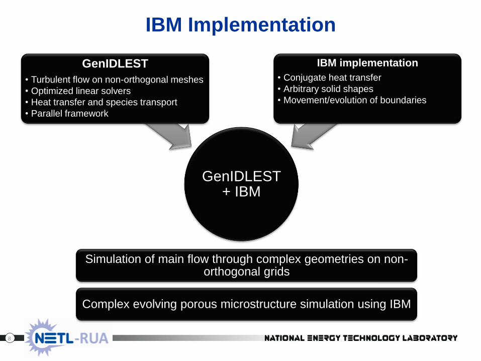
IBM Implementation

GenIDLEST+ IBM

GenIDLEST

• Turbulent flow on non-orthogonal meshes

• Optimized linear solvers

• Heat transfer and species transport

• Parallel framework

IBM implementation

• Conjugate heat transfer

• Arbitrary solid shapes

• Movement/evolution of boundaries

Simulation of main flow through complex geometries on non-orthogonal grids

Complex evolving porous microstructure simulation using IBM

8

Fluid Flow with IBM

Pressure coefficients obtained for steady flow

over a stationary cylinder

Lift coefficient comparison with experiments

obtained for an oscillating cylinder at Re = 200

Validations performed for stationary and

moving boundary cases for a variety of 2D

and 3D problems

Non-dimensional time

12 14 16 18 20-1

-0.5

0

0.5

1

y(t)

CL

- IBM

CL

- [5]

Angle

Cp

0 50 100 150-1.2

-1

-0.8

-0.6

-0.4

-0.2

0

0.2

0.4

0.6

0.8

1

1.2

1.4

Re = 10, calculation



Re = 10, [3]

Re = 20, [3]

Re = 40, [3]

9

Heat Transfer with IBM

Time-averaged local Nusselt number distribution

on a stationary cylinder at Re = 120 for iso-

thermal case

Comparison of temperature fields obtained in a

conjugate heat transfer setup between coannular

cylinders at various grid levels

Validations and comparisons with boundary

conforming code results performed check

different heat transfer BCs

Non-dimensional radial distance

No

n-d

imen

sio

nal te

mp

era

ture

A n g le ( )

Nu

ss

elt

nu

mb

er

(Nu

)

-1 5 0 -1 0 0 -5 0 0 5 0 1 0 0 1 5 0

2

4

6

8

1 0 IB M re s u lts

E x p e r im e n ta l re s u lts

L o c a l N u s s e lt n u m b e r d is tr ib u tio n ( tim e -a v e ra g e d )

R e = 1 2 0

[4]

10

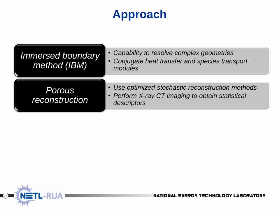
Approach







11

Porous Medium Reconstruction

• Use of stochastic

reconstruction method –

simulated annealing [6]

• Input – experimentally

determined auto-

correlation function (ACF)

• Initial – random field with

desired porosity

• Final – porous structure

with desired porosity and

auto-correlationA 2D porous medium generated with a porosity of

ε = 0.60

12

Porous Medium Reconstruction

Stochastic reconstruction of a 2D porous medium

with porosity of 0.75

13

Porous Flows with IBM

• Modified surface element

detection for porous

structures

• Input porous structure:

Binary information (fluid –

1, solid – 0)

• Test cases

– Comparison of pressure

drops with analytical

solutions

– Species diffusion through

porous particlesZoomed view of the velocity field around the porous

structure and the corresponding nodal identifications

Temperature contours in a porous channel

flow with conjugate heat transfer

14

Porous Flows with IBM

• Porous media used

– Square blocks randomly

placed in a channel flow

– “Porous channel” is

squeezed between the two

non-porous channels

– 2D random porous

structures generated using

simulated annealing

• Pressure drops obtained

using Darcy-Forchheimer

equation [7]

15

Approach









16

Species Diffusion

• Transport of species into

porous particles (2D)

– Square cavity with 15%

CO2 concentration at the

walls

– Zero gradient BC at the

porous medium walls

– Initial - 15% CO2 in air

outside

– Particle diameter – 500

microns

Diffusion of CO2 into a porous 2D particle

17

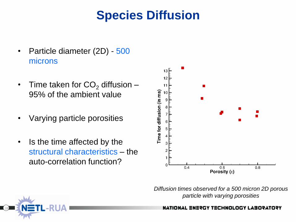
Species Diffusion

• Particle diameter (2D) - 500

microns

• Time taken for CO2 diffusion –

95% of the ambient value

• Varying particle porosities

• Is the time affected by the

structural characteristics – the

auto-correlation function?

Diffusion times observed for a 500 micron 2D porous

particle with varying porosities

18

Species Diffusion

• Variation with change in

the ACF

– Overlap distance between

the input structures (ε =

0.60)

Overlap Time for diffusion (ms)

0.6 D 7.995

0.8 D 7.246

1.0 D 6.01

1.2 D 7.709

19

Species Diffusion


the ACF



0.60)

– Size of the input structures

(ε = 0.75)Size (μm) Time for diffusion (ms)

50 6.85

100 6.66

150 6.911

200 7.29

20

Species Diffusion


the ACF



0.60)

– Size of the input structures

(ε = 0.75)

• No definite pattern

observed so far

– Simulations performed for ε

> 0.60, for which diffusion

time is in the asymptotic

range

Case Time for diffusion (ms)

1 6.85

2 6.66

3 6.911

4 7.29

Overlap Time for diffusion (ms)

0.6 D 7.995

0.8 D 7.246

1.0 D 6.01

1.2 D 7.709

21

Species Diffusion

Contour plots obtained from a 3D diffusion simulation

through a porous particle (ε = 0.45)

22

Major Achievements

• Capability to handle arbitrary 2-D and 3-D surface contours

– Validation for stationary and moving boundary problems

• Temperature BC for heat transfer studies into IBM framework

– Validation for uniform flow over a stationary cylinder

– Includes implementation of conjugate heat transfer

• Porous flow simulation

– Stochastic reconstruction of arbitrary porous structures

– Simulation and comparison with analytical results

– Species diffusion through 2D and 3D porous particles

23

Approach









• Could potentially lead to design of tailored microstructures to best achieve the adsorption process

Help improve CO2

capture

24

Future work

• Parallelization of IBM framework to enable faster computations (a major bottle-neck currently)

• Digital reconstruction of porous microstructure of typical sorbent particles through X-ray CT (or TEM/SEM) imaging

• Use of physical CO2 adsorption rates in simulations depending on the local surface conditions

• Spatio-temporal evolution of the porous microstructure with adsorption

25

Acknowledgements

• This financial support for this technical effort was

provided through the National Energy Technology

Laboratory – Regional University Alliance (NETL-RUA)

program.

• Multiphase Flow Research Group (MFRG) at NETL

26

References

1. DOE/NETL Advanced carbon dioxide capture R&D program: Technology update, September 2010

2. A general reconstruction algorithm for simulating flows with complex 3D immersed boundaries on Cartesian grids, Gilmonov, A., Sotiropoulos, F. and Balaras E., J. Comp. Phy., Vol. 191, pp. 660-669, 2003.

3. Numerical solutions of flow past a circular cylinder at Reynolds numbers up to 160, Park, J., Kwon, K. and Choi, H., KSME Int. J., Vol. 12, No. 6, pp. 1200-1205, 1998.

4. An immersed boundary finite-volume method for simulation of heat transfer in complex geometries, J. Kim and H. Choi, KSME Int. J., Vol. 18, No. 6, pp1026-1035, 2004.

5. Vortex wake and energy transitions of an oscillating cylinder at low Reynolds number, Stewart, B., Leontini, J., Hourigan, K. and Thompson, M.C., ANZIAM J., Vol. 46(E), pp. C181-C195, 2005.

6. A hybrid process-based and stocahstic reconstruction method of porous media, Politis, M.G., Kikkinides, E.S., Kainourgiakis, M.E. and Stubos, A.K., Microporous Mesoporous Mat., Vol. 110, pp. 92-99, 2008.

7. Direct simulation of forced convection flow in a parallel plate channel filled with porous media, Rahimian, M.H. and Pourshaghagy, Int. Comm. Heat Mass Transfer, Vol 29, No. 6, pp. 867-878, 2002.

27

Thank you!

Stochastic Reconstruction

Taken from Ref2

29

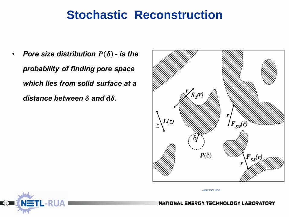
Stochastic Reconstruction

Taken from Ref2

30

Simulated annealing

31

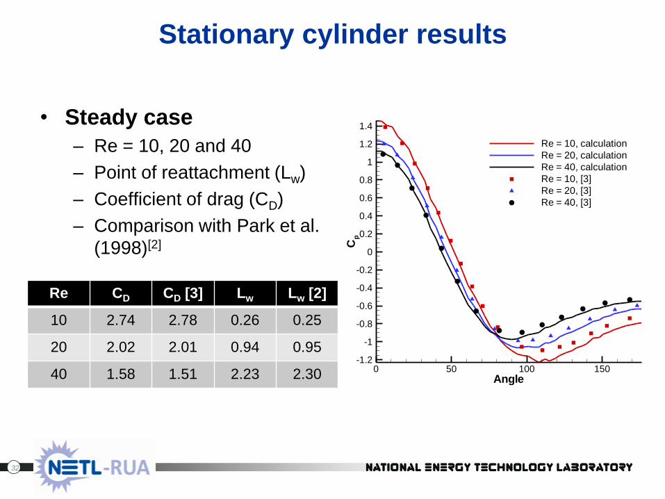
Stationary cylinder results

• Steady case

– Re = 10, 20 and 40

– Point of reattachment (Lw)

– Coefficient of drag (CD)

– Comparison with Park et al.

(1998)[2]

Re CD CD [3] Lw Lw [2]

10 2.74 2.78 0.26 0.25

20 2.02 2.01 0.94 0.95

40 1.58 1.51 2.23 2.30 Angle

Cp

0 50 100 150-1.2

-1

-0.8

-0.6

-0.4

-0.2

0

0.2

0.4

0.6

0.8

1

1.2

1.4




Re = 10, [3]

Re = 20, [3]

Re = 40, [3]

32

Stationary cylinder results

• Unsteady case

– Karman vortex street

– Re = 100, 150 and 200

– Strouhal number

comparison

Re = 150

Re St St [3]

100 0.166 0.16

150 0.185 0.18

200 0.198 0.20

x

y

20 22 24 26

12

14

16

18

33

Oscillating Cylinder

• Re = 200

• Frequency – 0.2

• Amplitudes – 0.2D and 0.7D

• Grid size of 0.00625D

• CL profile– Correct values predicted

– Compared with numerical results of Stewart et al.[5]

• Correct prediction of changed vortex shedding pattern for 0.7D amplitude

CL profile for 0.2D amplitude


12 14

-0.6

-0.4

-0.2

0

0.2

0.4

0.6

y(t)

CL

- IBM

CL

- [5]


12 14 16 18 20-1

-0.5

0

0.5

1

y(t)

CL

- IBM

CL

- [5]

CL profile for 0.7D amplitude

34

Arbitrary surface contours

• Implementation of IBM to

simulate flow around solid

bodies of arbitrary shapes

• Applicable to both 2-D and

3-D problems

Flow over an airfoil

35

Heat transfer with IBM

• Temperature BC for energy equation implemented in IBM

• Validation completed for uniform flow over a stationary

cylinder

• Constant heat flux and constant temperature conditions

implemented

• Implementation of conjugate heat transfer

• Results compared with exact solution

– Rotational flow between concentric cylinders

– Good comparison!

36

Heat transfer results

Re Experimental

results [5]

Present

10 1.80 1.83

40 3.28 3.18

120 5.69 5.56

Nusselt number comparisons (iso-thermal)

A n g le ( )

Nu

ss

elt

nu

mb

er

(Nu

)

-1 5 0 -1 0 0 -5 0 0 5 0 1 0 0 1 5 0

2

4

6

8

1 0 IB M re s u lts

E x p e r im e n ta l re s u lts

L o c a l N u s s e lt n u m b e r d is tr ib u tio n ( tim e -a v e ra g e d )

R e = 1 2 0

37

Conjugate heat transfer results

Immersed

boundary Radial distanceN

on

-dim

en

sio

nal t

em

pe

ratu

re

38

Porous flows with IBM

39

Porous flows with IBM

40

heat and mass transfer in porous co2 sorbent particles · heat and mass transfer in porous co 2...

Documents