drying of porous particles containing liquid mixtures in …765818/fulltext01.pdf · drying of...
TRANSCRIPT
Master’s Thesis in Chemical Engineeringfor Energy and the Environment
Stockholm, Sweden 2012
M A S O U D H A E R I N E J A D
Drying of Porous Particles containingLiquid Mixtures in a Continuous Vibrated
K T H C h e m i c a l S c i e n c ea n d E n g i n e e r i n g
Fluid Bed Dryer
Torkning av porösa partiklar innehållandevätskeblandningar i en vibrerande
!uidbäddtork

Drying of Porous Particles Containing Liquid
Mixtures in a Continuous Vibrated Fluid Bed Dryer
Masoud Haeri Nejad
Master Thesis
Department of Chemical Engineering and Technology
KTH, Royal Institute of Technology
Stockholm 2012

Sammanfattning Inverkan av driftparameter på torkning av sfäriska porösa partiklar som innehåller lösningsmedelblandningar som avdunstar i kväve i en kontinuerligt viberande fluidbädd-tork studerades. En simuleringsmodell baserad på den analytiska lösningen till värme- och materieöverföringsekvationerna användes och ändringar föreslogs. Fyra olika tärnar vätskeblandningar valdes: aceton-kloroform-metanol(ACM), etanol-2-propanolvatten,(EIpW), vatten-etanol-etylacetat (WEEa) och etanol-metyletylketon-toluen(EMekT). För den fasta fasen användes fysikaliska egenskaper liknande Pyrex. Sammansättnings- och temperatur-profiler visade att det inte finns något motstånd mot värmeöverföring i den fasta fasen och att värmeöverföringen sker mycket snabbare än materieöverförningen. Selektivitetsdiagram ritades. Resultaten indikerar att selektivititen är en viktig parmeter för att förutsäga beteendet vid torkning. Retentionsförhållandet användes som ett prestandamått. Dess variation med avseende på förändringar av driftsparmetrar, bland annat gasen hastighet och temperatur samt den fasta fasens temperatur och partikelstorlek, studerades. En modifiering av modellen undersöktes genom att införa en vätskehalts-beroende faktor för diffusionsmotståndet. Detta minskade värdena på retentionsförhållandena. Vibrationens inverkan på värme- och materieöverföring infördes genom att använda Sbrodov samband, och den resulterande effekten på retentionsförhållandet observerades. Nyckelord: analytisk lösning, arom retentionsförhållandet, flerkomponent materieöverföring, selektivetet, Fickian diffusiviteter, vibrerade fluidbäddtork
iii
Abstract
The influence of operation parameters on the drying of spherical porous particles containing a mixture of solvents evaporating into nitrogen in a continuously worked vibrated fluid-bed dryer was studied. A simulation based on the analytical solution to heat and mass transfer equations was applied and modifications were suggested.
Four different ternary liquid mixtures were selected: Acetone-Chloroform-Methanol (ACM), Ethanol-2-propanol-Water (EIpW), Water-Ethanol-Ethyl Acetate (WEEa) and Ethanol-Methylethylketone-Toluene (EMekT). For the solid, physical properties of Pyrex was used.
Comparison of composition- and temperature- profiles indicated that there is no resistance against heat transfer within the solid and that the heat transfer is much faster than mass transfer.
Selectivity diagrams were drawn. The results indicated that selectivity is an important parameter in predicting the drying behavior.
The retention ratio was studied as performance parameter. Its variation was studied in response to changes in operation parameters, including gas velocity and temperature, as well as solid temperature and particle size.
A modification to the model was examined by assuming a liquid-content-dependent diffusion resistance factor. It was observed that implementing such an assumption yields decreased values for retention ratios.
The effect of vibration on heat and mass transfer coefficients was included using a correlation suggested by Sbrodov and the resulting effect on retention ratio was examined.
Keywords: Analytical solution, aroma retention ratio, multicomponent mass transfer, selectivity, Fickian diffusivities, vibrated fluid-bed dryer.

iv
Acknowledgements This master thesis was carried out at the Division of Transport Phenomena at the Department of Chemical Engineering and Technology, KTH, Royal Institute of Technology. I would like to express my gratitude to my supervisor, Professor Joaquin Martinez de la Cruz for his support and guidance and for making this thesis possible. I also wish to say thanks to all who supported me in any respect during the project.
This thesis is dedicated to my family.
v
Table of Contents 1. INTRODUCTION __________________________________________________________ 1 1.1. BACKGROUND _________________________________________________________ 1 1.2. AIM AND SCOPE ________________________________________________________ 1 1.3. OUTLINE _____________________________________________________________ 1 2. LITERATURE REVIEW _____________________________________________________ 2 2.1. MULTICOMPONENT DRYING ______________________________________________ 2 2.2. VIBRATING FLUID-BED DRYERS __________________________________________ 4 3. MATHEMATICAL MODEL __________________________________________________ 6 3.1. EQUIPMENT MODEL_____________________________________________________ 6 3.1.1. MASS BALANCE FOR THE DRYER _________________________________________ 6 3.1.2. ENERGY BALANCE FOR THE DRYER ______________________________________ 7 3.2. MATERIAL MODEL _____________________________________________________ 7 3.2.1. GOVERNING EQUATIONS FOR A PARTICLE __________________________________ 7 3.2.2. HEAT AND MASS TRANSFER COEFFICIENTS ________________________________ 9 3.3. ANALYTICAL SOLUTION _________________________________________________ 9 3.4. SELECTIVITY AND RETENTION RATIO ______________________________________ 10 4. RESULTS AND DISCUSSION _______________________________________________ 11 4.1. GENERAL FEATURES ___________________________________________________ 11 4.1.1. CONCENTRATION AND TEMPERATURE PROFILES WITHIN THE PARTICLE _________ 12 4.1.2. LIQUID CONTENT AND TEMPERATURE PROFILES ALONG THE DRYER ___________ 13 4.1.3. FICKIAN DIFFUSIVITIES _______________________________________________ 14 4.1.4. EVAPORATION FLUXES ________________________________________________ 15 4.2. SELECTIVITY _________________________________________________________ 17 4.2.1. EFFECT OF INITIAL COMPOSITION _______________________________________ 17 4.2.2. EFFECT OF THE CHOICE OF DIFFERENT SYSTEMS ___________________________ 19 4.3. RETENTION RATIOS ____________________________________________________ 20 4.3.1. INFLUENCE OF INLET GAS TEMPERATURE AND VELOCITY ____________________ 21 4.3.2. INFLUENCE OF INLET SOLID TEMPERATURE _______________________________ 23 4.3.3. INFLUENCE OF PARTICLE SIZE __________________________________________ 24 4.3.4. INFLUENCE OF VARIABLE DIFFUSION RESISTANCE FACTOR __________________ 24 4.3.5. INFLUENCE OF VIBRATION INTENSITY ____________________________________ 27 5. CONCLUSIONS __________________________________________________________ 28 6. NOMENCLATURE _______________________________________________________ 29 7. REFERENCES ___________________________________________________________ 33 8. APPENDICES ___________________________________________________________ 36 8.1. DERIVATION OF THE ANALYTICAL SOLUTION TO THE MATERIAL MODEL ________ 36 8.2. VARIOUS GRAPHS _____________________________________________________ 40 8.2.1. SELECTIVITY VS. POSITION ALONG THE DRYER ____________________________ 40 8.2.2. PARTICLE AND GAS TEMPERATURES VS. POSITION ALONG THE DRYER _________ 42 8.2.3. LIQUID CONTENT VS. POSITION ALONG THE DRYER ________________________ 44 8.2.4. PARTICLE TEMPERATURE VS. LIQUID CONTENT ___________________________ 46 8.2.5. FICKIAN DIFFUSIVITIES ALONG THE DRYER _______________________________ 47 8.2.6. MOLAR EVAPORATION FLUXES ALONG THE DRYER _________________________ 49 8.2.7. LIQUID COMPOSITION ALONG THE DRYER ________________________________ 51 8.3. PHYSICAL PROPERTIES OF THE COMPONENTS AT 298K _________________________ 52 8.4. TABLE OF FIGURES _____________________________________________________ 53

1
1. INTRODUCTION
1.1. BACKGROUND Drying is a process used widely in chemical industry. A wide range of substrates including foodstuff, grains, wood, textile and leather are dried in different kinds of equipment based on different drying techniques (Mujumdar, 2007).Vaporization of water and its removal by air flow is the most common form of drying. However, drying can also involve non-aqueous liquids in pure form or as mixture components. Reduction of moisture to the desired level has proved to be dependent on a combination of factors including solid structure, liquid properties and the drying gas flow regime. The presence of several condensing components as the moisture content in the solid makes prediction of drying selectivity an important issue. Depending on whether retention or evaporation of one or more of the components is desired, one can think of the conditions that influence selectivity and its optimization during an industrial operation. In the present work, multicomponent- moisture drying inside a continuous vibrated fluid-bed dryer will be discussed. In these units, a shallow bed of porous solid particles wetted with a multicomponent mixture of solvents is fluidized by the flow action of the drying gas emerging from the impregnated surface of the moving plate carrying the particles along the dryer. The particles are difficult to fluidize due to surface moisture or the fineness of the particle size, therefore, mechanical vibrations are imposed to the drying bed in order to facilitate fluidization.
1.2. AIM AND SCOPE The objective of the present work is to use a model developed earlier for simulation of moisture removal in a continuous vibrated fluid-bed dryer. The model offers an analytical solution to the heat and mass transfer problem in multicomponent systems and will be used to predict multicomponent drying selectivity for several moisture systems. Effect of the variation in operation parameters will be studied using retention ratio as performance parameter. Moreover, assumptions will be made about the physics of the problem and based on that modifications will be made to the model.
1.3. OUTLINE This introduction is followed by a review of multicomponent drying theory and a description of the vibrating fluid-bed dryer in Chapter 2. Chapter 3 describes the mathematical formulation of the model. Chapter 4 discusses the general features of the simulation results including the effect of changing operation parameters on the final retention ratio. The effect of assuming a non-constant resistance factor for the diffusion coefficient and the effect of vibration intensity is also discussed. Finally, in Chapter 5, the conclusions are summarized and suggestions are given for further work.
2
2. LITERATURE REVIEW The purpose of this part is to describe the main characteristics of multicomponent drying as compared to single component drying. A description of vibrating fluid-bed dryers is also included.
2.1. MULTICOMPONENT DRYING Drying is a process for decreasing the liquid moisture of a solid substance. The liquid, which might be pure or composed of several components, is evaporated into a gas. This process involves changes in the energy content of the gas as well as in the remaining liquid. In the case of multicomponent liquid mixtures, drying can lead to changes in moisture composition, too. This change depends on the relative volatility of each component as well as on the diffusion rate of components within the liquid. A theory known as the film theory assumes that the resistance to mass and heat transfer lies entirely within a thin layer attached to the interphase surface. Here, the temperature and concentration gradients are created which act as the driving forces to heat and mass transfer from the bulk of each phase to the interphase boundary. Hence, gas-phase controlled or liquid-phase controlled mechanisms. For a more comprehensive treatment the reader is referred to (Reide & Schlünder, 1990) (Martinez, 1990) Evaporation of single- , two- or three component mixtures under stagnant or inert gas flow have already been observed experimentally (Birdi, 1989) (Dugas, 2005) (Hecht, 2000) (Moyle, 1997) (Murisic, 2011) (Poulard, 2003) (Prakash, 1980) (McGaughey, 2002), (Wilms, 2005)and successful models have been formulated to describe heat and mass transfer rates (Abou Al-Sood, 2008) (Dalmaz, 2005) (Evstropova, 1993) (Farid, 2003) (Hallet, 2011) (Hecht, 2000) (Kneer, 1993) (Korchinsky, 2009) (Lage, 1993) (Landry, 2007) (Lara-Urbaneja, 1981) (Marzo, 1986) (Murisic, 2011) (Negri, 1986) (Nesic, 1991) (Prakash, 1978) (Ravindaran, 1982) (Renksizbulut, 1991) (Rubel, 1981) (Stengele, 1999) (Tamim, 1995) (Tong, 1986) (Jiang, 2010).The solution of these models was normally done using numerical methods. Dried particles do not necessarily exist in well-defined solid-phase from the beginning. It is possible that the solids are already dispersed as solutions or slurries. By spraying the solution through fine nozzles, droplets are formed. The droplets evaporate into the surrounding gas environment and when they become rich in solid composition, the solids at the boundary surface begin to form crusts (shells) along the droplet outer surface (Nesic, 1991).The crust is usually not firm enough to hold all liquid content but contains cracks where vapors can escape. However, there are cases where robust crusts are formed which can cause a reduction of evaporation rate. It can also lead to elevated temperatures within the droplet until the encapsulated liquid boils. The pressure caused by expansion of the liquid into vapor can make the crust rupture abruptly in form of a micro-explosion. (Nesic, 1991) (Guerrier, 1998) (Burger, 2002), (Jiang, 2010) Most studies on evaporation are concentrated on predicting the surface temperature and the reduction in total mass and diameter of the droplets. The changes in diameter are often used to estimate evaporation rates. A treatment of the historical development of measuring techniques for the study of droplets is given by Wilms (2005). Due to the similarity between the drying behavior of a wetted spherical solid particle and a liquid droplet, the research findings from either area can be useful for the other.
3
Earlier models usually consider temperature change in liquid due to the fact that the temperature of the liquid is that of the wet bulb temperature for the gas but does not exceed the boiling point of the liquid even if the gas temperature exceeds the boiling point. (Pakowski, 1994) (Newbold & Amundson, 1973).Moreoever, due to the small size of the droplet and the turbulence of the flowing gas, internal resistance to mass and thermal transfer is neglected in these models. Abou Al-Sood (2008) investigating the effect of turbulence of the hot air stream on heat and mass transfer of a droplet, concluded that for high temperatures of around 1000°C radiation effects cannot be neglected and they account for up to 5% of the total heat transfer. In his single droplet model for a spray dryer, Dalmaz (2005) used Variable Grid Network and Variable Time Step algorithms for the constant- and falling- rate periods of evaporation, respectively. The simulation was shown to be successful in predicting evaporation of skimmed milk and colloidal silica, but not so for sodium deca-hydrate. This was attributed to the existence of non-idealities caused by liquid-solid interactions. Farid (2003) also modeled the drying of a droplet during spray drying of skimmed milk and colloidal silica. The evaporation was assumed to occur in the following steps: First, the droplet is quickly heated at constant mass. Then, it shrinks quickly at constant temperature. During the third step (crust formation) both mass and temperature change drastically and at the end, the temperature of the dried particle further increases. He calculated the Biot number to be greater than unity even for droplets as small as 200 µm in diameter and therefore assumed temperature gradients in the solid. He also identified thermal conductivity of the solid as an important contribution to drying rate. Murisic (2011) studied evaporation of droplets containing a binary mixture of water and 2-propanol on smooth silicon wafers where moving gas liquid boundary and moving liquid solid contact line occurred. A model was also developed for pure droplet evaporation taking Marangoni effect into consideration. Dugas (2005) in his attempt to achieve constant-contact-area drying regime during evaporation of droplets containing DNA on a hydrophobic flat surface used a mixture of surfactants and examined the effect of reduced ambient pressure as well as that of additives. It was concluded that introduction of internal liquid circulation plays an important role in achieving uniformly-sized dry spots. Wilms (2005) experimented with pure and two-component droplet evaporation into nitrogen and dry air atmospheres. Droplet diameters were in the range of 50 µm, which is typical for fuels. For pure components, size histories were used to estimate evaporation rates. Then a model was used to predict evaporation rates for binary and ternary mixtures. An analytical solution was derived for binary droplets. It was also observed that concentration gradients as predicted by diffusion-limit model did not occur in reality. They were, however, in good agreement with rapid-mixing model. This was concluded to be an indication of the significance of internal circulation within the droplet in enhancing mass transport. Poulard (2003) also considered the case where no pinning of the contact line occurs during droplet evaporation and concluded that both the volatility of the liquid and the properties of the wetting film left on the solid surface influence the evaporation kinetics. He also concluded
4
that the receding contact angle varies with the volatility but changes inversely with thickness of the wetting film. Landry (2007) studied argon nano-droplets using molecular dynamic simulations and observed that while at moderate atmospheric pressures, the square of droplet diameter changes linearly with time, at reduce pressures the droplet diameter decreases linearly with time. At higher pressures, for evaporation at supercritical temperatures, it is the number of atoms in the droplet that varies with time. Gusev and Sazhin (2011) studied the effect of moving boundary on evaporation of a Diesel fuel droplet. They suggested an explicit analytical solution to the Volterra integral equation of the second kind. This new solution was claimed to predict lower droplet surface temperatures and hence slower evaporation rates than those reported by earlier workers. McGaughey (2002) assumed the existence of temperature discontinuity at the gas-liquid interface. The claim is said to have been confirmed by statistical rate theory. This new finding revealed that the assumption of gas diffusion being the rate determining step as an explanation of the D2 law (i.e. assumption that the square of droplet diameter decreases linearly with time) for droplet size reduction, fails to give an accurate measure of the evaporation rate. The degree of inaccuracy was calculated to be in the range of 21%-37%. It was reported that incorporating the assumption of a temperature discontinuity improves the accuracy to 7%. It was concluded that assuming the interface kinetics as the rate determining step is more realistic than gas phase diffusion. Hallet (2011) used continuous thermodynamics vaporization model to predict biofuel droplet evaporation and concluded that when studying multicomponent mixtures, sufficient accuracy can still be attained if compounds of similar functional groups are considered as a single component. Korchinsky (2009) showed how using concentration-variable diffusivity instead of using mean constant values can affect mass flux values calculated for multicomponent rigid drops. It was concluded that for high mass transfer fluxes and/or large concentration gradients, the difference in mass flux values can be significant.
2.2. VIBRATING FLUID-BED DRYERS When small light-weight solid particles are exposed to gas flow, they can be transported along the flow path of the gas. The degree of the entrainment (carry-over) varies and can range from negligible to almost-complete entrainment (pneumatic transport). In industry, convective drying of solid particles encompasses all these situations. This has resulted in the implementation of different drying equipment and techniques. One classification divides dryers into three groups based on the degree of entrainment (Mujumdar, 2007):
1. Spray dryers and flash dryers( complete entrainment) 2. Fluid-bed dryers( partial entrainment) 3. Tray dryers and bed dryers ( small entrainment)
To collect entrained particles a cyclone is usually placed downstream. The gas flow can be co current, counter flow or cross flow with respect to flow direction of the solids.
5
Fluid- bed dryers come in different arrangements but the gas flow is normally cross-flow where the force due to the gas flow has to counteract and overcome the force of gravity before fluidization of particles can occur. As the gas flow increases, so does the pressure drop in the gas until when the particles originally disposed as a fixed bed, start to get separated from each other causing the overall bed volume to increase while the pressure drop remains unchanged at its maximum value. The superficial velocity corresponding to this flow rate amount is termed minimum fluidization velocity. (𝑢𝑚𝑓) . Beyond this velocity, the pressure drop decreases slightly while the bed expansion continues until it reaches its maximum value at bubbling point. Beyond bubbling point there is a possibility of total entrainment of the particles inside the gas flow (Land, 2012). However, not all the above stages are either achievable or desirable during a given drying process. One reason is due to the inherent tendency of particles of different sizes and densities towards fluidization. Geldart has classified fluidizability of the particles in their dry states into four groups: Group A (aeratable) and B (sand-like) are easier to fluidize due to their suitable range of size and density values, whereas group C particles are hard to fluidize because of their tendency to form agglomerates as a result of the cohesive inter-particle forces developed among these very fine particles. Starch and flour are examples of group C particles. Group D particles, on the other hand, are too big and too dense to fluidize. Some food grains represent this group which is also termed spoutable. Spouting is a form of channeling and uneven gas distribution through the bed of particles where a spout of gas is released at high intensity at certain locations across the upper surface of the bed (Mujumdar, 2007). Geldart classification is helpful in deciding the depth of the bed. While deep beds are common for group A and B particles, group C and D particle are advisable to be dried as shallow beds. Furthermore, for group C particles, mechanical vibration is applied in order to break up the agglomerates. Vibration is thought to have the additional advantage of increasing mass and heat transfer rates (Land, 2012). Fluid- bed dryers are designed either in circular or rectangular forms. The rectangular shape is used for shallow beds. A possible disadvantage of this geometry has been attributed to its size limitation to 8 x 1.6 m; beyond this size, the energy requirements are assumed to be prohibitively high (Land, 2012). Detailed description of the equipment can be found in standard reference books (Mujumdar, 2007). In a vibrated fluid-bed dryer operating in continuous mode, a stream of wet particles enters the dryer and leaves it at lower moisture content. Vibrations together with the flow of the drying gas are used to fluidize the particles. The particles move forward along the sloped surface of the dryer as a result of the vibration. Exhaust gas leaves the chamber from the top of the dryer. (Land, 2012) In the present work, a vibrated fluid- bed dryer is studied. The particles are assumed to be wetted with ternary liquid mixtures. The solid particles are assumed to be porous spheres and they possess physical properties similar to Pyrex. Moreover, the pore sizes are assumed to be not too fine to induce hygroscopic behavior. An upward cross-flow of nitrogen gas emerges from the impregnated surface of the rectangular conveyer-belt.
6
3. MATHEMATICAL MODEL Commercial software have been developed to solve sytems of partial differential equations involving coupled phenomena such as simultaneous heat and mass transfer. Some of them include NASTRAN, ABAQUS,ANSYS, and COMSOL. COMSOL MultiPhysics Module has been used to model phenomena related to drying. (Zeineldin, 2008) (Carin, 2006) (Curcio, 2009) (Floury, 2006). (Marin, 2006) (Takhar, 2009) The work of Pakowski is also notable where dryPAK and multidryPAK were developed to solve numerical calculations involved. (Pakowski Z. , 1999) (Pakowski Z. , 2000) The mathematical model applied in this work is the one reported by Picado (2011). The model is divided into two parts: the equipment model and the material model. The equipment model which summarizes mass and energy balances for the dryer is linked to the material model for the single particle by the values calculated for evaporation fluxes. Evaporation fluxes are determined using the basic assumptions of Maxwell-Stefan diffusion theory where the driving forces such as concentration gradient, pressure gradient or other external fields which contribute to diffusion are counter-balanced by friction forces arising from the interaction of the molecules passing by each other. This indicates that evaporation fluxes of each component is coupled to that of the other components and that various driving forces can affect mass transport. Moreover, since multicomponent evaporation involves different heats of evaporation for each component, assumption of a constant temperature equal to that of the wet bulb temperature of the gas does not apply. The work of Krishna to develop algorithms is one of the earliest examples of determining evaporation fluxes for multicomponent mixtures (Krishna & Standart, 1979). Later, Taylor improved the algorithm developed by Krishna (Taylor R. , 1982). This latter algorithm is the one which has been applied in the model used in the present work (Picado, 2011). In addition to wetted porous solid particles, this model has also been applied to simulate problems involving liquid films. (Gamero, 2006) (Luna, 2004).
3.1. EQUIPMENT MODEL (Picado, 2011) Complete mixing is assumed along the gas flow direction which is the direction perpendicular to that of the bed flow. Composition and temperature changes are therefore formulated in a single direction which is that of the bed movement. The bed is assumed to behave like a plug flow reactor so that no back-mixing is allowed (in real case there is certain amount of back mixing (Mujumdar, 2007)).Furthermore, stationary conditions are assumed for the bed. Mass and energy balances are formulated as per follows:
3.1.1. MASS BALANCE FOR THE DRYER Changes in liquid content along the dryer depend on the evaporation flux:
𝐹𝑠𝑑(𝑿)
𝑑𝑧= −𝑎𝑠(𝑴)𝑻�𝑮𝒈� (3.1)
7
Where Fs is the mass flow rate of dry solids per cross-section surface area, X is the moisture content of the solid in dry mass base, M is the molecular weight of the moisture mixture, as is the specific evaporation area per unit volume of the bed and Gg is the molar evaporation flux. To solve Equation (3.1), one needs to specify the inlet conditions. Moreover, an expression is needed for the evaporation flux. This expression, which depends on the drying kinetics, has been derived in the material model (Section 3.2). The following balance is used to give the change in gas humidity:
𝐹𝑔𝑑�𝒀𝒈� = −𝐹𝑠𝐻𝑏𝑑(𝑿)
𝑑𝑧 (3.2)
Where Fg is the mass flow of dry gas per unit cross section area, Yg is the gas humidity on dry basis and Hb is the bed height which is calculated as follows:
𝐻𝑏 =𝑆
𝑣𝜌𝑝(1 − 𝜀𝑝)(1 − 𝜀𝑏) (3.3)
Where S is the mass flow rate of dry solids, v is forward bed velocity, ρ is the density, and 𝜀𝑝 and 𝜀𝑏 are porosities of the particle and the bed, respectively.
3.1.2. ENERGY BALANCE FOR THE DRYER Neglecting heat losses, the energy balance over the same differential volume element as chosen for the mass balances yields:
𝑑𝐼𝑔 = −𝐻𝑏𝐹𝑠
𝐹𝑔
𝑑𝐼𝑠
𝑑𝑧 (3.4)
I is the enthalpy of the phases per unit dry mass. The subscripts s, b, and g refer to solid, bed and gas, respectively.
3.2. MATERIAL MODEL (Picado, 2011) The material model described below for the particle is used to calculate the evaporation flux, Gg which exists in Equation (3.1).
3.2.1. GOVERNING EQUATIONS FOR A PARTICLE In calculating mass transfer, diffusion is assumed to be the most significant mechanism, and therefore all other mechanisms are neglected. The equations are solved analytically; however, they are applied in increments along the dryer. Within each step, total concentration and transport coefficients are taken to be constant. In terms of spherical coordinates and assuming radial diffusion, mass transfer in the liquid mixture is expresses as:
𝜈𝜕(𝒙)
𝜕𝑧= [𝑫] �
𝜕2(𝒙)𝜕𝑟2 +
2𝑟
𝜕(𝒙)𝜕𝑟
� (3.5)
[𝑫] is the Fickian matrix of multicomponent mass transfer. It is calculated as the product of the inverse of B which is a matrix in terms of binary diffusion coefficients given by Maxwell-Stefan diffusion law and 𝚪 is a matrix containing the derivatives of activity coefficients with
8
respect to composition and serves to account for the thermodynamic non-ideality of the liquid mixture which is itself the result of interactions among the components (Taylor, 1981). See also Wesselingh & Krishna (2000), for more on multicomponent mass transfer.
Moreover, since the liquid is confined inside a porous particle, a resistance factor is also allowed for in the formulation of [𝑫]:
[𝑫] = 𝜄[𝑩]−1[𝚪]𝜁 (3.6)
ι is the resistance factor which for gases can be expressed in terms of tortuosity and constriction factors of a porous particle (Wesselingh & Krishna, 2000). The exponent ζ is included to correct for the non-idealities in the liquid mixture and it is determined by experiment. (Bandrowski, 1982).
Conduction, as an analogous mechanism to mass diffusion, is taken to be the mechanism responsible for heat transfer within the particle.
𝜈𝜕𝑇𝜕𝑧
= 𝐷ℎ �𝜕2𝑇𝜕𝑟2 +
2𝑟
𝜕𝑇𝜕𝑟
� (3.7)
where Dh is the thermal diffusivity. Equations (3.6) and (3.7) represent a system of partial differential equations complete with the following initial and boundary value conditions:
Initial conditions:
(𝒙) = �𝒙0(𝑟)� 0 ≤ 𝑟 ≤ 𝛿 𝑧 = 0 (3.8)
𝑇 = 𝑇0(𝑟) 0 ≤ 𝑟 ≤ 𝛿 𝑧 = 0 (3.9)
Boundary conditions at the center:
𝜕(𝒙)
𝜕𝑟= 0 𝑟 = 0 𝑧 > 0 (3.10)
Boundary conditions at the surface:
𝑐𝐿[𝑫]𝜕(𝒙)
𝜕𝑟= �𝑮𝒈 �𝑛−1
𝑟 = 𝛿 𝑧 > 0 (3.12)
−𝑘𝜕𝑇𝜕𝑟
= 𝑞 − (𝝀)𝑻 �𝑮𝒈� 𝑟 = 𝛿 𝑧 > 0 (3.13)
The evaporation fluxes can be written as: �𝑮𝑔� = [𝑲](𝐲𝛿 − 𝐲∞) (3.14)
𝐲𝛿 = 𝑲𝜸(𝒙)𝛿 (3.15)
𝜕𝑇𝜕𝑟
= 0 𝑟 = 0 𝑧 > 0 (3.11)

9
Where �𝑲 𝜸� is the matrix of equilibrium constants at the liquid-gas interphase and [K] is the matrix product[𝜷][𝒌][𝚵]. [𝒌] is the matrix of mass transfer coefficients for low-flux situation. To take into consideration the effect of finite mass transfer, [𝚵] is used as a correcting factor. Finally, [𝜷] which contains bootstrap relationship helps determine the composition of all the component of the system. In the present case, the fact that that nitrogen gas is the stagnant phase (i.e. not diffusing into the liquid) defines the bootstrap relation. For detailed treatment standard texts are suggested (Taylor & Krishna, 1993).Moreover, [K] is required to be transformed into a diagonal matrix so that Equation (3.5) can be solved analytically. For multicomponent systems, 𝑲𝒆𝒇𝒇 describes the matrix of effective transfer coefficients that produce the same evaporation fluxes at the free liquid surface as does Equation (3.14) and it is defined as: �𝑮𝑔� = [𝑲𝒆𝒇𝒇](𝐲𝛿 − 𝐲∞) (3.16)
𝑲𝒆𝒇𝒇 is a diagonal matrix with the following elements: 𝐾𝑖,𝑖,𝑒𝑓𝑓 = 𝐺𝑖,𝑔�𝑦𝑖,𝛿 − 𝑦𝑖,∞�
−1 𝑖 = 1,2, … , 𝑛 (3.17)
It should be remarked that in this model, changes of bulk gas conditions are neglected and the driving force is maintained by the changes in the gas composition at the surface of the solid. The conditions of the outlet gas are, however, calculated from the total balances in the equipment model.
3.2.2. HEAT AND MASS TRANSFER COEFFICIENTS Heat transfer by convection is formulated as: 𝑞 = ℎ𝑣Ξℎ(𝑇𝛿 − 𝑇∞) (3.17)
The value of heat transfer coefficient ℎ𝑣 is for low – mass transfer and is usually determined from empirical relations reported in terms of the Nusselt number:
𝑁𝑢𝑝 =ℎ𝑑𝑝
𝑘 (3.18)
The following relation for Nusselt number has been applied in the model.
𝑁𝑢𝑝 = 0.03𝑅𝑒𝑝1.3 𝑅𝑒𝑝 ≤ 500 (3.19)
𝑁𝑢𝑝 = 2 + 1.8𝑅𝑒𝑝0.5𝑃𝑟0.33 𝑅𝑒𝑝 > 500 (3.20)
Mass transfer coefficient was calculated using Chilton –Colborn analogy.
3.3. ANALYTICAL SOLUTION
Details of the derivation appear in the Appendix section, so that the transformed molar fraction is found to be:
(𝒖�) = 2 � 𝑒𝑥𝑝�−𝑫�𝝂𝑚2 𝜏�
∞
𝑚=1�
𝝂𝑚2 + 𝝃2
𝝂𝑚2 + 𝝃(𝝃 + 𝑰)
� sin(𝝂𝑚𝝃) �� 𝒖�0
1
0
(𝜁) sin(𝝂𝑚𝜁)𝑑𝜁� (3.22)

10
𝑢� and 𝐷� are uncoupled, transformed variables for molar composition vector and Fickian diffusivity matrix. 𝜁 and 𝜏 are dimensionless special coordinate variables corresponding to r and z ,respectively. 𝝂𝑚 is the vector of eigenvalues calculated by:
tan(𝝂𝑚) = 𝝃−1(𝝂𝑚) (3.23)
The integral in Equation (3.21) is a diagonal matrix and contains the values of the integral.
Analogously the transformed temperature is solved for to be:
Θ = 2 � 𝑒𝑥𝑝�−Κ𝜈𝑚,ℎ2 𝜏�
∞
𝑚=1�
𝜈𝑚,ℎ2 + 𝜉(𝑎 − 1)2
𝜈𝑚,ℎ2 + 𝑎(𝑎 − 1)
� sin�𝜈𝑚,ℎ𝜉� �� Θ0
1
0
(𝜁) sin�𝜈𝑚,ℎ𝜁�𝑑𝜁� (3.24)
With
tan�𝜈ℎ,𝑚� = (1 − 𝑎)−1�𝜈ℎ,𝑚� (3.25)
𝑎 =ℎ∗
𝑘𝑒𝑓𝑓𝛿 (3.26)
Where λ is the heat of vaporization and ℎ∗ is the heat transfer coefficient corrected for finite mass transfer:
ℎ∗ = ℎΞℎ (3.27)
Ξℎ is the Ackerman coefficient (Wesselingh & Krishna, 2000). h is calculated as described in Section 3.2.2.
After transformation of Equations (3.21) and (3.23) back into the original variables, the liquid compositions x and temperature T, are obtained. In addition to heat fluxes, evaporation fluxes Gg are also obtained and are used to solve Equation (3.1) in the equipment model.
3.4. SELECTIVITY AND RETENTION RATIO Selectivity is the difference between relative evaporation rate of a component and its composition in the liquid phase (Reide & Schlünder, 1990) (Martinez, 1990). 𝑆𝑖 = 𝑅𝑖 − 𝑥𝑖 (3.27)
Ri is the relative evaporation ratio of the component i and xi is the mean composition of the component in liquid phase. Evaporation selectivity can be affected by gas conditions, which includes its velocity and temperature as well as humidity (Reide & Schlünder, 1990). According to the theory of selective-diffusion (Thijssen, 1968), the more volatile components are the first to evaporate (they have positive selectivity) but then due to changes in viscosity, the diffusion coefficient decreases making the evaporation rate smaller but since the rate of decrease is greater for the volatile components,the selectivity becomes negative for the volatiles and positive for the less volatile component ( the sum of selectivities equals to zero).
11
As a result, the total remaining volatile content will be more than the value predicted thermodynamically.
Retention ratio is expressed as:
Retention ratio = (Xe,i/X0,i)/( Xe/X0). (3.28)
Xe and X0 are the initial and final liquid contents, respectively.
4. RESULTS AND DISCUSSION A code written in MATLAB is available which simulates the model (Picado, 2011). The program consists of several sub-routines; each containing functions to calculate one or more of the physical properties of the components. These functions include an algorithm reported by Taylor (1982) to calculate evaporation fluxes with diffusion through stationary air as a bootstrap relationship and linearized theory (Stewart & Prober, 1964) to evaluate the matrix of corrections factors. Heat transfer coefficients at zero-mass transfer rate were computed by correlations from Kunii and Levenspiel (1991) and binary diffusion coefficients were predicted using the methods reported by Fuller et al. (1966). Physical properties of pure components and mixtures were evaluated using methods described by Poling et al. (2000). Activity coefficients were calculated according to the Wilson equation with parameters taken from Gmehling and Onken (1982). Vapor pressures of pure liquids were computed using Antoine equation. In liquid phase, the method of Bandrowski and Kubaczka (1982) suggested for determining the Maxwell-Stefan diffusion coefficients was applied and an empirical exponent value of 0.5 was used for all liquid systems. Physical properties of Pyrex were used for the solid phase. Selectivity diagrams were drawn; retention ratios were calculated, and together, they were used to assess the performance of drying for 4 different ternary liquid systems.
4.1. GENERAL FEATURES Simulations were performed for four selected ternary liquid mixtures: Acetone -Chloroform-Methanol (ACM), Ethanol-2-propanol-Water (EIpW), Water-Ethanol-Ethyl Acetate (WEEa) and Ethanol-Methylethylketone-Toluene (EMekT). Some useful physical properties of the components are summarized in Appendix 8.3. The initial conditions in terms of component compositions are not the same for all systems. That is because in one case, for small values of volatile composition, the code went unstable (the case with EMekT system), therefore, higher volatile composition had to be chosen. In another case, the volatiles depleted much earlier than the particles arrived at the end of the dryer (WEEa). In this case, a shorter dryer length was selected. Table below summarizes the initial compositions of the moisture and the dryer lengths.

12
System Components x1 x2 x3 Dryer Length [m] Acetone, Chloroform, Methanol 0.15 0.15 0.70 0.8 Ethanol, 2-propanol,Water 0.15 0.15 0.70 0.8 Water, Ethanol, Ethyl Acetate 0.33 0.33 0.34 0.5 Ethanol, Methylethylketone, Toluene 0.33 0.33 0.34 0.8 The effect of initial composition on selectivity was verified for different initial compositions of EIpW system. The complete set of results for all systems is presented in the graphs in Appendix8.2. Below, the general features are discussed using the system Ethanol, 2-Propanol, Water (EIpW) as an example.
4.1.1. CONCENTRATION AND TEMPERATURE PROFILES WITHIN THE PARTICLE
Figure 1 Temperature versus dimensionless position in the particle (left); ethanol composition versus dimensionless position in the particle (right) for the system: Ethanol, 2-propanol, Water. Inlet solid temperature: 298 K, initial composition: [0.15 0.15] As shown in Figure 1, the temperature profile across the particle diameter remains relatively flat whereas a steep concentration gradient is established for each component (e.g. ethanol in Figure 1). These results indicate that there is no resistance towards heat transfer as compared to the mass transfer resistance. Therefore, it can be concluded that heat transfer occurs much faster than mass transfer in the solid particles and that the heat and mass transfer effects can be studied separately.

13
4.1.2. LIQUID CONTENT AND TEMPERATURE PROFILES ALONG THE DRYER Below is the temperature profile for the gas leaving the dryer and the particle temperature along the dryer for the system EIpW:
Figure 2 Mean Temperature of the particle and the outgoing gas for the system: Ethanol, 2-propanol, Water
Tg0 =343K, Ts0=298K, x0 = [0.15 0.15]
As the gas flows over the particles, its temperature decreases sharply as it delivers its sensible heat as latent heat to vaporize the liquid. Meanwhile, the temperature of the liquid also decreases when the heat delivered by the gas is not enough to support the high evaporation rate at the beginning. Therefore, some of the heat of evaporation is supplied by the liquid mixture within the solid. As the particles proceed through the dryer, the evaporation rate decreases when the volatiles content is depleted and so does the required heat for vaporization so that now the situation becomes manageable for the gas and there will be little or no change in temperature in either the gas or the liquid phases. Under this stationary situation it can be assumed that the heat provided by the gas is sufficient to vaporize the liquid.
14
4.1.3. FICKIAN DIFFUSIVITIES
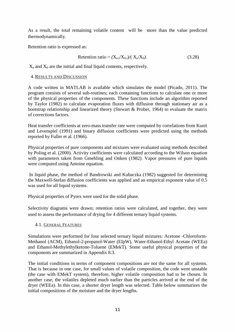
Below is the diffusion coefficient diagram within the dryer for the system EIpW for two different initial compositions:
x0= [0.15 0.15] x0= [0.33 0.33]
Figure 3 Changes for Fickian diffusivities along the dryer for the system: Ethanol, 2-Propanol, Water at two different initial compositions
It can be observed that as the particle moves along the dryer the main diffusion coefficients D11 and D22 decrease. The magnitude of the cross diffusion elements is indicative of interactions among the mixture components.
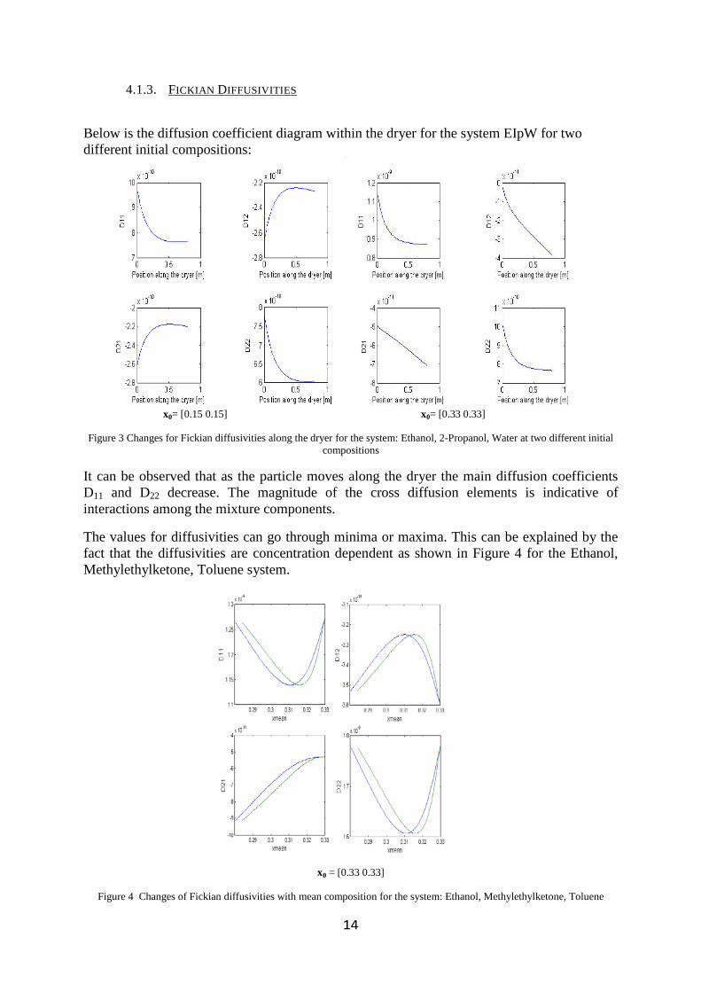
The values for diffusivities can go through minima or maxima. This can be explained by the fact that the diffusivities are concentration dependent as shown in Figure 4 for the Ethanol, Methylethylketone, Toluene system.
x0 = [0.33 0.33]
Figure 4 Changes of Fickian diffusivities with mean composition for the system: Ethanol, Methylethylketone, Toluene

15
This observation can be explained in terms of the matrix Γ which is a function of activity coefficients. The variation in the magnitude of the activity coefficients depends on the degree of non-ideality of the mixture and is an indicator of their mutual interactions. This matrix as mentioned earlier is multiplied by matrix B which is a function of Maxwell-Stefan diffusion coefficients to produce the matrix of Fickian diffusivities. (Krishna, 1976). Therefore, the variation in Fickian diffusivities is also due to the non-idealities of the mixture. The changes in diffusivity values can affect evaporation rates too. This is discussed in the next section.
4.1.4. EVAPORATION FLUXES Below are the molar evaporation rates for the two systems: Ethanol, 2-Propanol, Water (EIpW) and Ethanol, Methylethylketone, Toluene (EMekT) with initial conditions as mentioned in Section 4.1.
(a) (b)
Figure 5 Molar evaporation fluxes for the systems: Ethanol, 2-propanol, Water (a) and Ethanol, Methylethylketone, Toluene (b)
As shown in Figure 5a, the initial evaporation rate of water in EIpW system is higher than the evaporation rate for the more volatile components, ethanol and 2-propanol. It is also observed for the system EMekT in Figure 5b that although the evaporation rate is initially lower for the less volatile component (toluene) but as the drying proceeds its evaporation rate increases so much so that it exceeds those of the two more volatile components ,ethanol and methylethylketone. This can be explained by referring to the diffusivity values in Figure 6 and Figure 7.
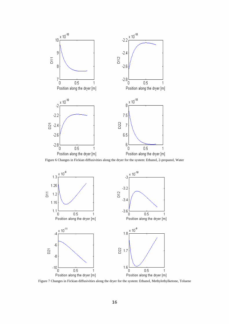
16
Figure 6 Changes in Fickian diffusivities along the dryer for the system: Ethanol, 2-propanol, Water
Figure 7 Changes in Fickian diffusivities along the dryer for the system: Ethanol, Methylethylketone, Toluene
17
Comparison of the results in Figure 7 with those in Figure 5 reveals that the evaporation rates follow the same trend as the changes in the D11 and D22, the main diffusivities. Also, one can note that the minimum in evaporation value for toluene occurs at the same dryer position as when the main diffusivity is a minimum. As discussed earlier, the shape of diffusivity graph is an indication of the characteristic intermolecular interactions within each system and moreover, it is a strong function of composition changes. Therefore, numerous shapes are imaginable for evaporation curves.
4.2. SELECTIVITY
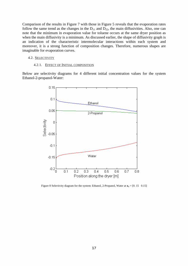
4.2.1. EFFECT OF INITIAL COMPOSITION Below are selectivity diagrams for 4 different initial concentration values for the system Ethanol-2-propanol-Water:
Figure 8 Selectivity diagram for the system: Ethanol, 2-Propanol, Water at x0 = [0. 15 0.15]

18
Figure 9 Selectivity diagram for the system: Ethanol, 2-Propanol, Water at x0 = [0. 33 0.17]
Figure 10 Selectivity diagram for the system: Ethanol, 2-Propanol, Water at x0 = [0. 17 0.33]
19
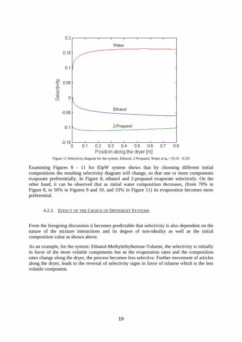
Figure 11 Selectivity diagram for the system: Ethanol, 2-Propanol, Water at x0 = [0.33 0.33]
Examining Figures 8 - 11 for EIpW system shows that by choosing different initial compositions the resulting selectivity diagram will change, so that one or more components evaporate preferentially. In Figure 8, ethanol and 2-propanol evaporate selectively. On the other hand, it can be observed that as initial water composition decreases, (from 70% in Figure 8, to 50% in Figures 9 and 10, and 33% in Figure 11) its evaporation becomes more preferential.
4.2.2. EFFECT OF THE CHOICE OF DIFFERENT SYSTEMS
From the foregoing discussion it becomes predictable that selectivity is also dependent on the nature of the mixture interactions and its degree of non-ideality as well as the initial composition value as shown above.
As an example, for the system: Ethanol-Methylethylketone-Toluene, the selectivity is initially in favor of the more volatile components but as the evaporation rates and the composition rates change along the dryer, the process becomes less selective. Further movement of articles along the dryer, leads to the reversal of selectivity signs in favor of toluene which is the less volatile component.

20
Figure 12 Selectivity diagram for the system: Ethanol, Methylethylketone, Toluene at x0 = [0.33 0.33]
4.3. RETENTION RATIOS The observations also included comparing changes in retention ratios, as a performance parameter, against changes in gas and liquid conditions, as operational parameters. Tables in each section summarize the influence of the given operation parameter on retention ratio.

21
4.3.1. INFLUENCE OF INLET GAS TEMPERATURE AND VELOCITY Depending on whether the mass transfer is controlled mainly by the gas phase or the liquid phase within the solid, the effectiveness of the parameters that can affect selectivity, varies.
Table 1 Influence of inlet gas temperature on retention ratio. ι= 1, u = 1.5 m/s, L = 0.8 m, x10=x20= 0.15
Components Retention Ratio
Tg01=326K Tg02=343K Tg03=360K Acetone 1.2474 1.4439 1.8007
Chloroform 0.9814 1.1049 1.3392
Methanol 0.9188 0.7439 0.4181
Table 2 Influence of inlet gas temperature on retention ratio. ι= 1, u = 1.5 m/s, L = 0.8 m, x10=x20= 0.15
Components Retention Ratio
Tg01=326K Tg02=343K Tg03=360K Ethanol 0.8699 0.8583 0.8496
2-propanol 0.9442 0.9314 0.9197
Water 1.1112 1.1267 1.1398
Table 3 Influence of inlet gas temperature on retention ratio. ι= 1, u = 1.5 m/s, L = 0.5 m, x10=x20= 0.33
Components Retention Ratio
Tg01=326K Tg02=343K Tg03=360K Water 1.5581 1.7505 2.0264
Ethanol 1.6233 1.8429 2.1566
Ethyl Acetate 0.5729 0.4233 0.2094
Table 4 Influence of inlet gas temperature on retention ratio. ι= 1, u = 1.5 m/s, L = 0.8 m, x10=x20= 0.33
Components Retention Ratio
Tg01=326K Tg02=343K Tg03=360K Ethanol 0.8890 1.0488 1.4832
MEK 1.0684 1.2549 1.7524
Toluene 1.0019 0.7828 0.1940 Comparison of the Tables 1-4 indicates that except for the system: Ethanol, 2-propanol, Water (EIpW), the other three systems exhibit significant sensitivity towards the changes in gas temperature. This means that the system EIpW is for the most part liquid phase controlled while mass transfer in the other systems are mostly gas-phase controlled.

22
It is, therefore, expected that similar trend should be observed when inlet gas velocity is changed. Tables 5-8 summarize the effect of changing the inlet gas velocity on retention ratio.
Table 5 Influence of inlet gas velocity on retention ratio. ι= 1, Tg0= 343K , L = 0.8 m, x10=x20= 0.15
Components Retention Ratio
ug01=1.35m/s ug02=1.50m/s ug03=1.65m/s Acetone 1.2674 1.4439 1.7767
Chloroform 0.9915 1.1049 1.3344
Methanol 0.9029 0.7439 0.4313
Table 6 Influence of inlet gas velocity on retention ratio. ι= 1, Tg0=343K, L = 0.8 m, x10=x20= 0.15
Components Retention Ratio
ug01=1.35m/s ug02=1.50m/s ug03=1.65m/s Ethanol 0.8672 0.8583 0.8552
2-propanol 0.9395 0.9314 0.9255
Water 1.1160 1.1267 1.1326
Table 7 Influence of inlet gas velocity on retention ratio. ι= 1, Tg0=343K, L = 0.5 m, x10=x20= 0.33
Components Retention Ratio
ug01=1.35m/s ug02=1.50m/s ug03=1.65m/s Water 1.5387 1.7505 2.0815
Ethanol 1.6094 1.8429 2.2059
Ethyl Acetate 0.5838 0.4233 0.1734
Table 8 Influence of inlet gas velocity on retention ratio. ι= 1, Tg0=343K, L = 0.8 m, x10=x20= 0.33
Components Retention Ratio
ug01=1.35m/s ug02=1.50m/s ug03=1.65m/s Ethanol 0.8829 1.0488 1.4009
Methylethylketone 1.1026 1.2549 1.5888
Toluene 0.9789 0.7828 0.3582
As expected, the system EIpW does not react significantly to the changes in gas flow conditions.
23
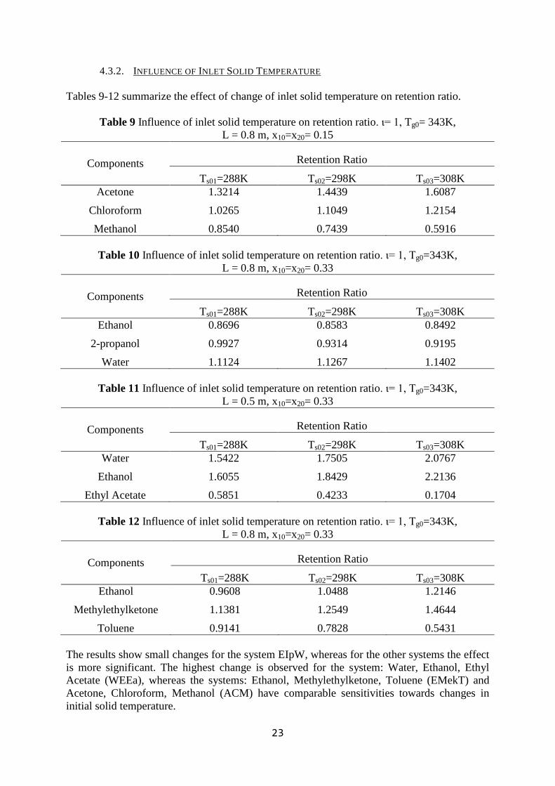
4.3.2. INFLUENCE OF INLET SOLID TEMPERATURE Tables 9-12 summarize the effect of change of inlet solid temperature on retention ratio.
Table 9 Influence of inlet solid temperature on retention ratio. ι= 1, Tg0= 343K, L = 0.8 m, x10=x20= 0.15
Components Retention Ratio
Ts01=288K Ts02=298K Ts03=308K Acetone 1.3214 1.4439 1.6087
Chloroform 1.0265 1.1049 1.2154
Methanol 0.8540 0.7439 0.5916
Table 10 Influence of inlet solid temperature on retention ratio. ι= 1, Tg0=343K, L = 0.8 m, x10=x20= 0.33
Components Retention Ratio
Ts01=288K Ts02=298K Ts03=308K Ethanol 0.8696 0.8583 0.8492
2-propanol 0.9927 0.9314 0.9195
Water 1.1124 1.1267 1.1402
Table 11 Influence of inlet solid temperature on retention ratio. ι= 1, Tg0=343K, L = 0.5 m, x10=x20= 0.33
Components Retention Ratio
Ts01=288K Ts02=298K Ts03=308K Water 1.5422 1.7505 2.0767
Ethanol 1.6055 1.8429 2.2136
Ethyl Acetate 0.5851 0.4233 0.1704
Table 12 Influence of inlet solid temperature on retention ratio. ι= 1, Tg0=343K, L = 0.8 m, x10=x20= 0.33
Components Retention Ratio
Ts01=288K Ts02=298K Ts03=308K Ethanol 0.9608 1.0488 1.2146
Methylethylketone 1.1381 1.2549 1.4644
Toluene 0.9141 0.7828 0.5431 The results show small changes for the system EIpW, whereas for the other systems the effect is more significant. The highest change is observed for the system: Water, Ethanol, Ethyl Acetate (WEEa), whereas the systems: Ethanol, Methylethylketone, Toluene (EMekT) and Acetone, Chloroform, Methanol (ACM) have comparable sensitivities towards changes in initial solid temperature.

24
4.3.3. INFLUENCE OF PARTICLE SIZE Tables 13-16 summarize the effect of change in particle size on retention ratio.
Table 13 Influence of particle size on retention ratio. ι= 1, Tg0=343K, L = 0.8 m, x10=x20= 0.15
Components Retention Ratio
dp1=2.93e-3m dp2=3.00e-3m dp3=3.45e-3m Acetone 1.4766 1.4439 1.3145
Chloroform 1.1066 1.1049 1.0967
Methanol 0.7298 0.7439 0.8007
Table 14 Influence of particle size on retention ratio. ι= 1, Tg0=343K, L = 0.8 m, x10=x20= 0.15
Components Retention Ratio
dp1=2.93e-3m dp2=3.00e-3m dp3=3.45e-3m Ethanol 0.8536 0.8583 0.8831
2-propanol 0.9293 0.9314 0.9423
Water 1.1307 1.1267 1.1053
Table 15 Influence of particle size on retention ratio. ι= 1, Tg0=343K, L = 0.5 m, x10=x20= 0.33
Components Retention Ratio
dp1=2.93e-3m dp2=3.00e-3m dp3=3.45e-3m Water 1.7820 1.7505 1.6006
Ethanol 1.8787 1.8429 1.6730
Ethyl Acetate 0.3989 0.4233 0.5392
Table 16 Influence of particle size on retention ratio. ι= 1, Tg0=343K, L = 0.8 m, x10=x20= 0.33
Components Retention Ratio
dp1=2.93e-3m dp2=3.00e-3m dp3=3.45e-3m Ethanol 1.0401 1.0488 1.0837
Methylethylketone 1.2647 1.2549 1.2118
Toluene 0.7795 0.7828 0.7985
4.3.4. INFLUENCE OF VARIABLE DIFFUSION RESISTANCE FACTOR Resistance factor for diffusion was studied in two parts. First, the simulation was run for different constant values of resistance factor. The resulting graphs did show some effect on

25
evaporation fluxes in general. The results were not regular and therefore they are not included in this work. Next, it was assumed that resistance is not constant throughout the drying process but it is a function of the liquid content. It was assumed that tortuosity is inversely proportional to liquid content so that as the drying proceeds, the overall resistance factor which is the ratio of constriction on tortuosity increases. This assumption was verified using the retention ratio and the selectivity diagram and is shown for the systems EIpW and EMekT:
1. EIpW system a) Retention ratio:
Table 17 Influence of diffusion resistance factor on retention ratio. Tg0=343K, L = 0.8 m, x10=x20= 0.15
Components Retention Ratio
ι=1 ι=1/Xi Ethanol 0.8583 0.8416
2-propanol 0.9314 0.9264
Water 1.1267 1.1394
b) Selectivity Diagram:
Figure 13 Effect of variable diffusion resistance factor (dashed) on selectivity compared to a constant factor (ι=1) (solid) on selectivity for the system Ethanol, 2-propanol, Water
The results indicate less retention for the volatile components and therefore less selectivity. This can be observed in the selectivity diagram.
26
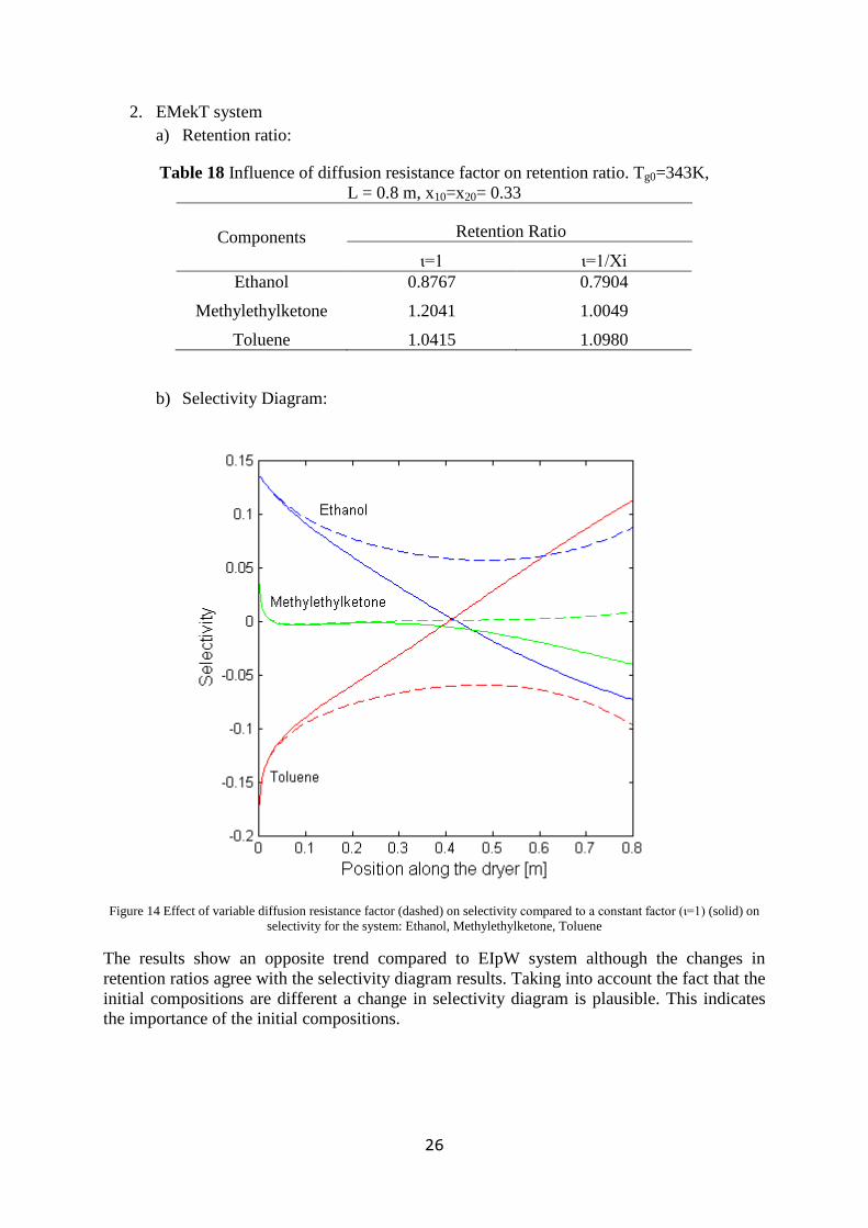
2. EMekT system a) Retention ratio:
Table 18 Influence of diffusion resistance factor on retention ratio. Tg0=343K, L = 0.8 m, x10=x20= 0.33
Components Retention Ratio
ι=1 ι=1/Xi Ethanol 0.8767 0.7904
Methylethylketone 1.2041 1.0049
Toluene 1.0415 1.0980
b) Selectivity Diagram:
Figure 14 Effect of variable diffusion resistance factor (dashed) on selectivity compared to a constant factor (ι=1) (solid) on selectivity for the system: Ethanol, Methylethylketone, Toluene
The results show an opposite trend compared to EIpW system although the changes in retention ratios agree with the selectivity diagram results. Taking into account the fact that the initial compositions are different a change in selectivity diagram is plausible. This indicates the importance of the initial compositions.

27
4.3.5. INFLUENCE OF VIBRATION INTENSITY Vibration was studied using two different approaches. In the first trial, vibration was incorporated into the model as a correction factor in the input data. The resulting retention ratios were, however, irregular and no conclusion could be drawn. In the second case, the original relation used for calculation of Nusselt number (Section 3.2.2) was replaced by the relation reported by Sbrodov: (Pakowski et al., 1984) 𝑁𝑢 = 0.142𝑅𝑒. Γ0.04 (4.1)
Γ = 𝐴𝜔2/𝑔 (4.2)
𝜔 = 2𝜋𝑓 (4.3)
A is vibration amplitude (m), f is frequency (Hz), g is the acceleration due to gravity (g= 9.8 m/s2). This new relationship includes a term involving the dimensionless vibration intensity, Γ. Γ was altered by changing the frequency values and retention ratios were calculated. The results obtained this time were regular but the trends can be opposite for different systems. The results are summarized in Tables 19-22.
Table 19 Influence of vibration frequency on retention ratio. ι= 1, Tg0=343K, L = 0.5 m, x10=x20= 0.15, dp=3e-3m
Components
Retention Ratio
original f1=12.9Hz f2=16.1Hz f3=19.7Hz Acetone 1.4439 0.8654 1.2862 1.3031
Chloroform 1.1049 0.9380 1.0029 1.0133
Methanol 0.7439 1.1181 0.8865 0.8717
Table 20 Influence of vibration frequency on retention ratio. ι= 1, Tg0=343K, L = 0.8 m, x10=x20= 0.15, dp=3e-3m
Components
Retention Ratio
original f1=12.9Hz f2=16.1Hz f3=19.7Hz f4=51.6Hz Ethanol 0.8583 0.8654 0.8641 0.8630 0.8583
2-propanol 0.9314 0.9380 09369 0.9360 0.9315
Water 1.1267 1.1181 1.1196 1.1209 1.1266
28
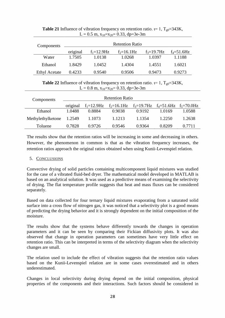
Table 21 Influence of vibration frequency on retention ratio. ι= 1, Tg0=343K, L = 0.5 m, x10=x20= 0.33, dp=3e-3m
Components
Retention Ratio
original f1=12.9Hz f2=16.1Hz f3=19.7Hz f4=51.6Hz Water 1.7505 1.0138 1.0268 1.0397 1.1188
Ethanol 1.8429 1.0452 1.4304 1.4551 1.6021
Ethyl Acetate 0.4233 0.9540 0.9506 0.9473 0.9273
Table 22 Influence of vibration frequency on retention ratio. ι= 1, Tg0=343K, L = 0.8 m, x10=x20= 0.33, dp=3e-3m
Components
Retention Ratio
original f1=12.9Hz f2=16.1Hz f3=19.7Hz f4=51.6Hz f5=70.0Hz Ethanol 1.0488 0.8884 0.9038 0.9192 1.0169 1.0588
Methylethylketone 1.2549 1.1073 1.1213 1.1354 1.2250 1.2638
Toluene 0.7828 0.9726 0.9546 0.9364 0.8209 0.7711 The results show that the retention ratios will be increasing in some and decreasing in others. However, the phenomenon in common is that as the vibration frequency increases, the retention ratios approach the original ratios obtained when using Kunii-Levenspiel relation.
5. CONCLUSIONS Convective drying of solid particles containing multicomponent liquid mixtures was studied for the case of a vibrated fluid-bed dryer. The mathematical model developed in MATLAB is based on an analytical solution. It was used as a predictive means of examining the selectivity of drying. The flat temperature profile suggests that heat and mass fluxes can be considered separately. Based on data collected for four ternary liquid mixtures evaporating from a saturated solid surface into a cross flow of nitrogen gas, it was noticed that a selectivity plot is a good means of predicting the drying behavior and it is strongly dependent on the initial composition of the moisture. The results show that the systems behave differently towards the changes in operation parameters and it can be seen by comparing their Fickian diffusivity plots. It was also observed that change in operation parameters can sometimes have very little effect on retention ratio. This can be interpreted in terms of the selectivity diagram when the selectivity changes are small. The relation used to include the effect of vibration suggests that the retention ratio values based on the Kunii-Levenspiel relation are in some cases overestimated and in others underestimated. Changes in local selectivity during drying depend on the initial composition, physical properties of the components and their interactions. Such factors should be considered in

29
design of drying applied to multicomponent mixtures. The same conclusions can be applied to droplet evaporation. Further work can include examining the effect of preloading of the drying gas on the selectivity and the study of azeotropes.
6. NOMENCLATURE a Dimensionless variable defined in Equations (3.25) -
as Specific evaporation area per bed volume m2/m3
A Amplitude of vibration m
b Dimensionless variable defined in Equations (A.11) -
B Matrix in Equation (3.6) m-2s
B Dryer width m
c Total molar concentration kmol m-3
dp Particle diameter m
D Mass transport coefficient m2s-1
D Matrix of multicomponent diffusion coefficients m2s-1
Dh Thermal Diffusivity m2s-1
𝑫� Diagonal matrix of eigenvalues of 𝑫� -
𝑫� Dimensionless matrix of multicomponent diffusion coefficients -
𝑓 Frequency of vibration s-1(Hz)
𝐹 Mass flow per cross section kg s-1 m-2
𝑔 Acceleration due to gravity ms-2
𝐺 Molar flux kmol s-1m-2
𝑮 Vector of molar fluxes kmol s-1m-2
ℎ Zero-flux heat transfer coefficient Wm-2K-1
ℎ∗ Convective heat transfer coefficient defined as ℎ∗ = ℎΞℎ Wm-2K-1
𝐻𝑏 Bed height m
𝐼 Enthalpy per unit mass, on dry basis Jkg-1
𝐈 Identity matrix -
𝐽 Diffusion flux kmol s-1m-2
𝐉 Matrix of diffusion fluxes kmol s-1m-2

30
𝑘 Thermal conductivity Wm-1K-1
𝑘𝑚 Mass transfer coefficient kmol s-1m-2
𝐤 Matrix of zero-flux mass transfer coefficients kmol s-1m-2
𝐊𝑒𝑓𝑓 Diagonal matrix with elements defined in Equation (3.39) kmol s-1m-2
𝐊𝛾 Matrix of equilibrium constants -
𝐿 Dryer length m
𝑚 Mass kg
𝑀 Molecular weight of the moisture kgkmol-1
𝑛 Number of components -
𝐏 Modal matrix of eigenvalues of 𝑫� -
𝑞 Heat flux Wm-2
𝑟 Radial coordinate m
𝑆 Flow of dry solids kg s-1
𝑡 Time s
𝑇 Temperature K
𝑢 Transformed liquid molar fraction variable -
𝑢𝑔 Gas velocity ms-1
𝐮� Vector of transformed liquid molar fraction -
𝑣 Forward velocity of the bed of solids ms-1
𝑉 Mass flow of dry air kg s-1
𝑤 Molar fraction -
𝒘 Vector of molar fractions -
𝑥 molar fraction in liquid -
𝐱 Vector of liquid compositions -
𝑋 Moisture content , dry basis -
𝑦 Gas molar fraction -
𝐲 Vector of gas compositions -
𝐲𝑏 Vector related to bulk gas molar fractions in Equation (A.10) -
𝑌 Gas humidity , dry basis kg kg-1
31
𝑧 Length coordinate along dryer m
Greek letters 𝛃 Bootstrap matrix -
𝛾 Activity coefficient -
𝛄 Matrix of activity coefficients -
Γ𝑣 Vibration intensity [≡ 𝐴𝜔2/𝑔] -
𝛿 Particle radius m
𝛿𝑖𝑗 Kronecker delta -
𝜀 Porosity -
𝜁 Dimensionless radial coordinate/radius -
𝜃 Dimensionless temperature -
Θ Transformed temperature -
𝜄 Coefficient in Equation (3.6) -
Κ Dimensionless heat transfer diffusivity -
𝜆 Heat of vaporization Jkmol-1
𝛌 Vector of heats of vaporization Jkmol-1
𝜈ℎ,𝑚 Eigenvalue roots related to heat transfer -
𝜈𝑚 Eigenvalue roots related to mass transfer -
𝛎𝑚 Diagonal matrix of eigenvalues related to mass transfer -
𝝃 Matrix defined in Equation (A.28) -
𝝃𝒇 Matrix defined in Equation (A.26) -
Ξℎ Correction factor on the heat transfer coefficient -
𝚵 Matrix of correction factors on the mass transfer coefficients -
𝜌 density kg m-3
𝜏 Dimensionless length in Equation (A.1) -
𝝓 Coefficient defined in Equation (A.10) -
𝜔 Angular frequency[≡ 2𝜋𝑓] rads-1

32
Subscripts 𝑏 bed
𝑒 exit
𝑒𝑓𝑓 Effective value
𝑔 gas
𝑖𝑗 Binary, position in matrix
𝑖𝑘 Binary, position in matrix
𝑘 Time-counting index
𝑙 liquid
𝑛 Number of components
𝑝 particle
𝑠 solid
𝛿 interface
∞ Gas bulk
0 Inlet or initial
Superscript T Transpose of a matrix or a column vector

33
7. REFERENCES Abou Al-Sood, M. M. (2008). Droplet heat and mass transfer in a turbulent hot air stream.
International Journal of Heat and Mass Transfer, 51, 1313-1324. Bandrowski, J. (1982). On Prediction of Diffusivities in Multicomponent Liquid Systems.
Chem. Eng. Sci., 1309-1313. Birdi, K. (1989). A Study of the Evaporation Rates of Small Water Drops Placed on a Solid
Surface. J. Phys. Chem., 93, 3702-3703. Burger, M. (2002). A Multicomponent Droplet Evaporation Model for Real Aviation Fuels at
Elevated Pressures. ILASS-Europe-2002. Zaragoza. Carin, M. (2006). Numerical Simulation of Moving Boundary Problems with an ALE
Method. Validation in the Case of a Free Surface or a Moving Boundary Front. COMSOL Users Conference. Paris, France.
Carslaw, H., & J.C.Jaeger. (1959). Conduction of Heat in Solids (2nd ed.). London, UK: Oxford University Press.
Curcio, S. (2009). Transport Phenomena and Shrinkage Modeling During Convective Drying of Vegetables. COMSOL Conference. Milan, Italy.
Dalmaz, N. (2005, August). Modeling and Numerical Analysis of Single Drop Drying. Dugas, V. (2005). Droplet Evaporation Study Applied to DNA Chip. Langmuir, 21, 9130-
9136. Evstropova, E. (1993). Boundary Layer and Heat Transfer in a Two-phase Gas-Evaporation
Medium. UDC, 331-337. Farid, M. (2003). A new approach to modelling of single droplet drying. Chem.Eng. Sci., 58,
2985-2993. Floury, J. (2006). Modeling the Coupled Mass Transfer Phenomena During Osmotic
Dehydration of Fresh and Frozen Mango Tissues. COMSOL Users Conference. Paris. Fuller, E. (1966). A New Method for Prediction of Binary Gas-Phase Diffusion Coefficients.
Ind. Eng. Chem., 58(5), 19-27. Gusev, I. (2011). The Effects of the Moving Boundary on the Heating of Evaporating
Droplets. 24th European Conference on Liquid Atomization and Spray Systems (ILASS – Europe 2011). Estoril, Portugal.
Hallet, W. (2011). Modelling biodiesel droplet evaporation using continuous thermodynamics. Fuel, 90, 1221-1228.
Hecht, J. (2000). Spray Drying: Influence of Developing Drop Morphology on Drying Rates and Retention of Volatile Substances. 1. Single-Drop Experiments. Ind. Eng. Chem. Res., 39, 1756-1765.
Hecht, J. (2000). Spray Drying: Influence of Developing Drop Morphology on Drying Rates and Retention of Volatile Substances. 2. Modeling. Ind. Eng. Chem., 39, 1766-1774.
Hofmann, H. (1928). Formuation of Nitrocelullose Lacquers. Ind. Eng. Chem., 20(7), 687-693.
Hofmann, H. (1932). Evaporation Rates of Organic Liquids. Ind. Eng. Chem., 24(2), 135-140. Jiang, X. (2010). Numerical Simulation of Ethanol-Water-NaCl Droplet Evaporation. Ind.
Eng. Chem. Res., 49, 5631-5643. Kneer, R. (1993). Diffusion controlled evaporation of a multicomponent droplet: theoretical
studies on the importance of variable liquid properties. Int. J. Heat Mass Transfer, 36(9), 2403-2415.
Korchinsky, W. (2009). Multicomponent mass transfer in films and rigid drops: The influence of concentration-variable diffusivity. Chem. Eng. Sci., 64, 433-442.
Krishna, R. (1976). A Multicomponent Film Model Incorporating a General Matrix Method of Solution to the Maxwell-Stefan Equations. AIChE Journal, 22(2), 383-389.
34
Krishna, R., & Sandart, L. (1979). Mass and Energy Transfer in Multicomponent Systems. Chem. Engng. Commun., 3, 201.
Lage, P. (1993). Multicomponent heat and mass transfer for flow over a droplet. Int. J. Heat Mass Transfer, 36(14), 3573-3581.
Landry, E. (2007). Droplet Evaporation: A molecular dynamics Investigation. Journal of Applied Physics, 102(124301), 1-7.
Lara-Urbaneja, P. (1981). Theory of Transient Multicomponent Droplet Vaporization in a Convective Field. Eighteenth Symposium ( International ) on Combustion.
Law, C. (n.d.). Theory of Conductive, Transient, Multicomponent Droplet Vaporization. Lewis, W. (1935). Evaporation of Lacquer Solvents. Ind. Eng. Chem., 27(12), 1395-1396. Luna, F. (1998). Stability of the Dynamical System Describing Isothermal Gas-Phase-
Controlled Drying of Ternary Mixtures. Drying Technology, 16(9-10), 1807-1825. Marin, T. (2006). Solidification of a Liquid Metal Droplet Impinging on a Cold Surface.
COSMOL Users Conference. Boston,U.S.A. Martinez, J. (1990). Convective Drying of Solids Wetted with Multicomponent Solvent
Mixtures. PhD Thesis,KTH, Royal Institute of Technology. Stockholm, Sweden. Martinez, J. (1991). Gas-phase Controlled Convective Drying of Solids Wetted with
Multicomponent Liquid Mixtures. Chem. Eng. Sci., 46(9), 2235-2252. Marzo, M. D. (1986). Evaporation of aWater Droplet Deposited on a Hot High Thermal
Conductivity Solid Surface. U.S. Department of Commerce National Bureau of Standards.
McGaughey, A. (2002). Temperature discontinuity at the surface of an evaporating droplet. Journal of Applied Physics, 91(10), 6406-6415.
Michalski, J. (2009). An Analysis of Heat Conduction with Phase Change during the Solidification of Copper. COMOL Conference. Boston,U.S.A.
Moyle, A. (1997). Laboratory Studies of Water Droplet Evaporation Kinetics. 12th Int.Confer.on Clouds and Precip. 1996,Zurich,Switzerland
Mujumdar, A. (2007). Handbook of Industrial Drying (Third ed.). (A. Mujumdar, Ed.) Boca Raton: CRC Press.
Murisic, N. (2011). On evaporation of sessile drops with moving contact lines. J. Fluid Mech., 679, 219-246.
Negri, E. (1986). Multicomponent Mass Transfer in Spherical Rigid Drops. Chem. Eng. Sci., 41(9), 2401-2406.
Nesic, S. (1991). Kinetics of Droplet Evaporation. Chem. Eng. Sci., 46(2), 527-537. Newbold, F., & N.R.Amundson. (1973). A Model for Evaporation of A Multicomponent
Drop. AIChE Journal, 19(1), 22-30. Pakowski, Z. (1992). The Evaporation of Ternary Liquid Azeotropes to Air. 8th International
Drying Symposium ( IDS '98). Montreal, Quebec, Canada. Pakowski, Z. (1994). Drying of Solids Containing Multicomponent Moisture: Recent
Developments. 9th International Drying Symposium ( IDS '94). Gold Coast, Australia. Pakowski, Z. (1997). Drying of White Sugar in Fluid Bed: Simulation and Design of
Industrial Scale Dryers-Coolers. Drying Technology, 15(6-8), 1881-1892. Pakowski, Z. (1999). Simulation of the Process of ConvectiveDrying : Identification of
Generic Computation Routines and Their Implementation in a Computer Code dryPAK. Computers and Chemical Engineering Supplement, S719-S722.
Pakowski, Z. (2000). Simulation of Convective Drying of Multicomponent Moisture in a Computer Code MultiPAK. European Symposium on Computer Aided Process Engineering-10.
35
Pakowski, Z. A. (1984). Theory and Application of Vibtated beds and vibrated fluid beds for drying processes. In A. Mujumdar, Advances in Drying (Vol. 3, p. 288). USA: Hemisphere Publishing Corporation.
Picado, A. (2011). An Analytical Solution Applied to Heat and Mass Transfer in a Vibrated Fluidised Bed Dryer. Licenciate Thesis, , KTH,Stockholm.
Poulard, C. (2003). Freely Receding Evaporating Droplets. Langmuir, 19, 8828-8834. Prakash, S. (1978). Liquid Fuel Droplet Heating with Internal Circulation. Int. J. Heat Mass
Transfer, 21, 885-895. Prakash, S. (1980). Theory of Convective Droplet Vaporization with Unsteady Heat Transfer
in the Circulating Liquid Phase. Int. J. Heat Mass Transfer, 23, 253-268. Ravindaran, P. (1982). Multicomponent Evaporation of Single Aerosol Droplets. Journal of
Colloid and Interface Science, 85(1), 278-288. Reide, T., & E.U.Schluender, 1. (1990). Selective Evaporation of a Ternary Mixture
Containing One Nonvolatile Component with Regard to Drying Processes. Chem. Eng. Process., 28, 151-163.
Reide, T., & Schluender, E. (1990). Selective Evaporation of a Binary Mixture into Dry or Humidified Air. Chem. Eng. Process, 27, 83-93.
Renksizbulut, M. (1991). A Mass Transfer Correlation for Droplet Evaporation in High-Temperature Flows. Chem. Eng. Sci., 46(9), 2351-2358.
Renksizbulut, M. (1993). Multicomponent droplet evaporation at intermediate Reynolds numbers. Int. J. Heat Mass Transfer, 36(11), 2827-2835.
Rubel, G. (1981). On the Evaporation Rates of Multicomponent Oil Droplets. Journal of Colloid and Interface Science, 81(1), 188-195.
Stengele, J. (1999). Experimental and theoretical study of one- and two- component droplet vaporization in a high pressure environment. Int. J. Heat Mass Transfer, 42, 2683-2694.
Stewart, W. 1. (1973). Multicomponent Mass Transfer in Turbulent Flow. AIChE Journal, 19(2), 398-400.
Stewart, W., & R.Prober, 1. (1964). Matrix Calculation of Multicomponent Mass Transfer in Isothermal Systems. Ind. and Eng. Chemistry Fundam., 3(3), 224-235.
Takhar, P. (2009). Drying of Corn Kernels: From Experimental Images to Multiscale Multiphysics Modeling. CoMSOL Conference. Boston,U.S.A.
Tamim. (1995). A Continuous Thermodynamics Model for Multicomponent Droplet Vaporization. Chem.Eng. Sci., 50(18), 293-2942.
Taylor, R. (1981). Coupled Heat and Mass Transfer in Multicomponent Systems: Solution of the Maxwell-Stefan Equations. Letters in Heat and Mass Transfer, 8, 405-416.
Taylor, R. (1982). Film Models for Multicomponent Mass Transfer: Computational Methods-II The Linearised Theroy. Computers and Chemical Engineering, 6, 69-75.
Taylor, R. (1982). Solution of the Linearized Equations of Multicomponent Mass Transfer. Ind. Eng. Chem. Fundam., 21, 407-413.
Taylor, R., & D.R.Webb, 1. (1981). Film Models for Multicomponent mass Transfer; Computational Methods: The Exact Solution of the Maxwell-Stefan Equations. Computers and Chemical Engineering, 5, 61-73.
Taylor, R., & Krishna.R. (1993). Multicomponent Mass Transfer. John Wiley and Sons, Inc. Thijssen, H. W. (1968). Retention of Aromas in drying liquid foods. De Ingenieur(85), 45-56. Tong, A. (1986). Multicomponent Droplet Vaporization in a High Temperature Gas.
Combustion and Flame, 66, 221-235. Wesselingh, J., & R.Krishna. (2000). Mass Transfer in Multicomponent Mixtures. Delft: Delft
University Press. Wilms, J. (2005). Evaporation of Multicomponent Droplets. Stuttgart: Universität Stuttgart.
36
8. APPENDICES
8.1. DERIVATION OF THE ANALYTICAL SOLUTION TO THE MATERIAL MODEL (Picado, 2011)
By introducing the following dimensionless variables, Equations (3.5) and (3.7) can be made dimensionless:
𝜏 =𝑧𝐿 𝜁 =
𝑟𝑅 𝜃 =
𝑇 − 𝑇∞
𝑇𝑔0 − 𝑇∞ (A.1)
𝜕(𝑥)𝜕𝜏
= [𝐷𝑑] �𝜕2(𝑥)
𝜕𝜁2 +2𝜁
𝜕(𝑥)𝜕𝜁
� 𝜕𝜃𝜕𝜏
= κ �𝜕2𝜃𝜕𝜁2 +
2𝜁
𝜕𝜃𝜕𝜁
� (A.2)
[𝑫𝑑] =𝐿𝑫𝜈𝛿2 𝜅 =
𝐿𝐷ℎ
𝜈𝛿2 (A.3)
The inlet and boundary conditions are:
Initial conditions:
(𝒙) = �𝒙0(𝜁)� 0 ≤ 𝜁 ≤ 1 𝜏 = 0 (A.4)
𝑇 = 𝑇0(𝜁) 0 ≤ 𝜁 ≤ 1 𝜏 = 0 (A.5)
Boundary conditions at the center:
𝜕(𝒙)
𝜕𝜁= 0 𝜁 = 0 𝜏 > 0 (A.6)
𝜕𝜃𝜕𝜁
= 0 𝜁 = 0 𝜏 > 0 (A.7)
Boundary conditions at the surface:
−𝜕(𝒙)
𝜕𝜁= 𝝓𝒙 + 𝒚𝑏 𝜁 = 1 𝜏 > 0 (A.8)
−𝜕𝜃𝜕𝜁
= 𝑎𝜃 + 𝑏 𝜁 = 1 𝜏 > 0 (A.9)
𝝓 =𝐿
𝜈𝛿𝑐𝐿𝑫𝑑
−1�𝑲𝑲𝛾�𝑛−1
𝒚𝑏 =𝐿
𝜈𝛿𝑐𝐿𝑫𝑑
−1{𝑲𝒚∞}𝑛−1 (A.10)
And
𝑎 =ℎ∗
𝑘𝑒𝑓𝑓𝛿 𝑏 =
−𝑎(𝝀)�𝑮𝑔�ℎ∗�𝑇𝑔 − 𝑇0�
(A.11)
The subscript n-1 indicates that the matrix product consists of the first n-1 column and rows of the original matrix product.

37
Equation (A.2) may now be transformed into ones describing linear flow in one direction by introducing the following new dependent variables
(𝑢) = 𝜁([𝜙](𝑥) + [𝑦𝑏′ ]) Θ = 𝜁(𝑎𝜃 + 𝑏) (A.12)
Equations (A.2) become:
𝜕(𝑢)
𝜕𝜏= �𝑫�� �
𝜕2(𝑢)𝜕𝜁2 �
𝜕Θ𝜕𝜏
= κ𝜕2Θ𝜕𝜁2 (A.13)
With
�𝑫�� = [𝝓][𝑫𝑑][𝝓]−1 (A.14)
The new inlet and boundary conditions are:
Initial conditions:
(𝒖) = �𝒖0(𝜁)� 0 ≤ 𝜁 ≤ 1 𝜏 = 0 (A.15)
Θ = Θ0(𝜁) 0 ≤ 𝜁 ≤ 1 𝜏 = 0 (A.16)
Boundary conditions at the center:
𝒖 = 0 𝜁 = 0 𝜏 > 0 (A.17)
Θ = 0 𝜁 = 0 𝜏 > 0 (A.18)
Boundary conditions at the surface:
𝜕(𝒖)
𝜕𝜁+ (𝝓 − 𝑰)𝒖 = 𝟎 𝜁 = 1 𝜏 > 0 (A.19)
𝜕Θ𝜕𝜁
+ (𝑎 − 1)Θ = 0 𝜁 = 1 𝜏 > 0 (A.20)
Where I is the diagonal identity matrix. The compositions in Equation (A.13) can be de-coupled through the similarity transformation
𝑫� = 𝑷𝑫�𝑷−1 (A.21)
𝒖� = 𝑷−1𝒖 (A.22)
The matrix P is the modal matrix whose columns are the eigenvectors of 𝑫� and 𝑫� is a diagonal matrix of its eigenvalues. The transformation yields:
𝜕(𝑢�)
𝜕𝜏= �𝐷��
𝜕2(𝑢�)𝜕𝜁2 (A.23)
With initial and boundary conditions:

38
(𝒖�) = �𝒖�0(𝜁)� 0 ≤ 𝜁 ≤ 1 𝜏 = 0 (A.24)
𝒖� = 0 𝜁 = 0 𝜏 > 0 (A.25)
𝜕(𝒖�)
𝜕𝜁= −𝝃𝒇(𝒖�) 𝜁 = 0 𝜏 > 0 (A.26)
Where
�𝝃𝒇� = [𝑷]([𝝓] − [𝑰])[𝑷]−1 (A.27)
Since the solution demands 𝝃𝒇 to be a diagonal matrix, a new diagonal matrix 𝝃 is defined so that it satisfies:
𝝃𝒇(𝒖�) = 𝝃(𝒖�) (A.28)
Giving the new boundary conditions:
𝜕(𝒖�)
𝜕𝜁= −𝝃(𝒖�) (A.29)
Equation (A.29) is not explicitly dependent on temperature and can be solved separately. Under the assumption that the matrix 𝝃 is constant the de-coupled differential equation can be solved by the method of variable separation. The solution reported by Carslaw and Jaeger (1959) is:
(𝑢�) = 2 � 𝑒𝑥𝑝�−𝐷�𝜈𝑚2 𝜏�
∞
𝑚=1�
𝜈𝑚2 + 𝜉2
𝜈𝑚2 + 𝜉(𝜉 + 1)
� sin(𝜈𝑚𝜉) �� 𝑢�0
1
0
(𝜁) sin(𝜈𝑚𝜉)𝑑𝜁� (A.30)
To preserve the formalism of matrix product, the integral in Equation (A.30) is a diagonal matrix that contains the value of the integral. The eigenvalues in Equation (A.30) are defined implicitly by:
tan(𝜈𝑚) = 𝜉−1(𝜈𝑚) (A.31)
Finally, 𝒖� is transformed back to obtain the liquid composition:
𝒙 = 𝝓−1(𝑷𝒖�𝜁
− 𝒚𝑏) (A.32)
At the center of the particle, where = 0 , the composition is undetermined and the expression must be evaluated as a limit. The limit of the expression is related to the derivative of the transformed composition with respect to the dimensionless space.
lim𝜁→∞
�(𝑢�)
𝜁� = lim
𝜁→∞�
𝑑(𝑢�)𝑑𝜁
� (A.33)

39
By evaluating the derivative of Equation (A.30) at 𝜁 = 0 :
lim𝜁→∞
�𝑑(𝑢�)
𝑑𝜁 � = � 𝑒𝑥𝑝�−𝐷�𝜈𝑚2 𝜏�
∞
𝑚=1�
𝜈𝑚2 + 𝜉2
𝜈𝑚2 + 𝜉(𝜉 + 1)
� �� 𝑢�0
1
0
(𝜁) sin(𝜈𝑚𝜁)𝑑𝜁� (A.34)
Equation (A.32) provides the mole fraction of n-1 component s in the liquid. The mole fraction of the nth component is calculated taking advantage of:
𝑥𝑛 = 1 − � 𝑥𝑗
𝑛−1
𝑗=1 (A.35)
For the temperature:
Θ = 2 � 𝑒𝑥𝑝�−Κ𝜈𝑚,ℎ2 𝜏�
∞
𝑚=1�
𝜈𝑚,ℎ2 + 𝜉(𝑎 − 1)2
𝜈𝑚,ℎ2 + 𝑎(𝑎 − 1)
� sin�𝜈𝑚,ℎ𝜉� �� Θ0
1
0
(𝜁) sin�𝜈𝑚,ℎ𝜁�𝑑𝜁� (A.36)
With eigenvalues obtained from: tan�𝜈ℎ,𝑚� = (1 − 𝑎)−1�𝜈ℎ,𝑚� (A.37)
Upon transforming back to temperature:
𝑇 = 𝑇𝑔 −�𝑇𝑔 − 𝑇0�
𝑎�
Θ𝜁
− 𝑏� (A.38)
The values at the center are calculated using a similar relation between the limits as in Equation (A.33):
lim𝜁→∞
�Θ𝜁
� = lim𝜁→∞
�𝑑Θ𝑑𝜁
� (A.39)
Applied to Equation (A.36):
lim𝜁→∞
�𝑑Θ𝑑𝜁
� = 2 � 𝑒𝑥𝑝�−Κ𝜈𝑚,ℎ2 𝜏�
∞
𝑚=1�
𝜈𝑚,ℎ2 + 𝑎(𝑎 − 1)2
𝜈𝑚,ℎ2 + 𝑎(𝑎 − 1)
� �� Θ0
1
0
(𝜁) sin�𝜈𝑚,ℎ𝜁�𝑑𝜁� (A.40)
Although the solution is only valid for constant physical properties, the variation of coefficients for the whole process can be taken into account by a piecewise application of the analytical solution along the process trajectory. That is, by performing the solution in successive steps where the final conditions of the previous step are used to calculate the coefficients and as initial condition of the next step.

40
8.2. VARIOUS GRAPHS
8.2.1. SELECTIVITY VS. POSITION ALONG THE DRYER
Figure 15 Selectivity Diagram for the system: Acetone, Chloroform, Methanol at x0 = [0.15 0.15]
Figure 16 Selectivity Diagram for the system: Ethanol, 2-propanol, Water at x0 = [0.15 0.15]
41
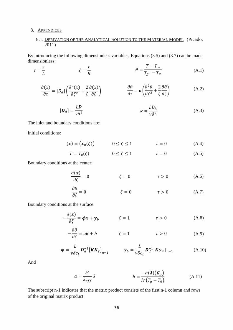
Figure 17 Selectivity Diagram for the system: Water, Ethanol, Ethyl Acetate at x0 = [0.33 0.33]
Figure 18 Selectivity Diagram for the system: Ethanol, Methylethylketone, Toluene at x0 = [0.33 0.33]
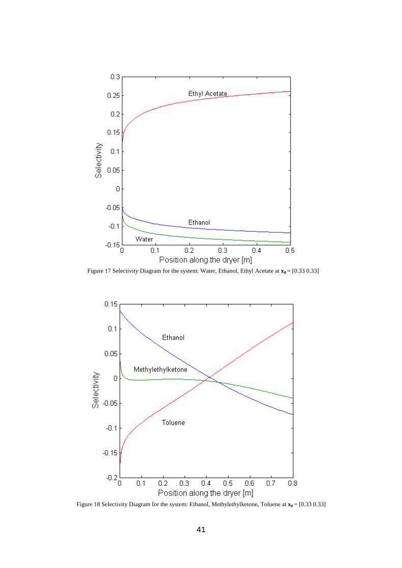
42
8.2.2. PARTICLE AND GAS TEMPERATURES VS. POSITION ALONG THE DRYER
Figure 19 Mean temperature of the particle and outgoing gas for the system: Acetone, Chloroform, Methanol
Figure 20 Mean temperature of the particle and outgoing gas for the system: Water, Ethanol, Ethyl Acetate
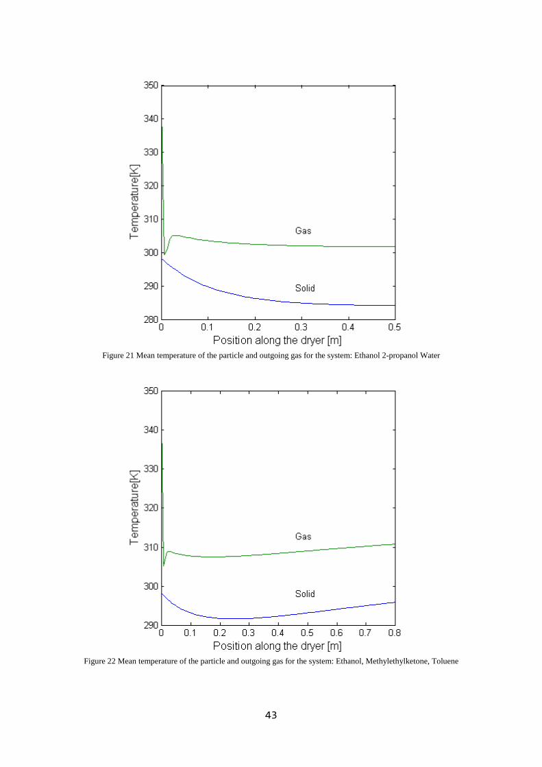
43
Figure 21 Mean temperature of the particle and outgoing gas for the system: Ethanol 2-propanol Water
Figure 22 Mean temperature of the particle and outgoing gas for the system: Ethanol, Methylethylketone, Toluene

44
8.2.3. LIQUID CONTENT VS. POSITION ALONG THE DRYER
Figure 23 Changes in liquid content along the dryer for the system: Acetone, Chloroform, Methanol
Figure 24 Changes in liquid content along the dryer for the system: Ethanol, 2-propanol, Water

45
Figure 25 Changes in liquid content along the dryer for the system: Water, Ethanol, Ethyl Acetate
Figure 26 Changes in liquid content along the dryer for the system: Ethanol, Methylethylketone, Toluene
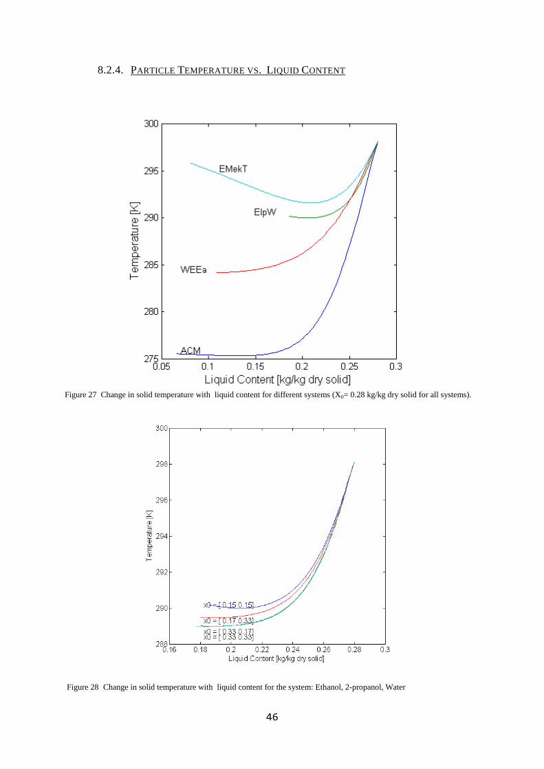
46
8.2.4. PARTICLE TEMPERATURE VS. LIQUID CONTENT
Figure 27 Change in solid temperature with liquid content for different systems (X0= 0.28 kg/kg dry solid for all systems).
Figure 28 Change in solid temperature with liquid content for the system: Ethanol, 2-propanol, Water
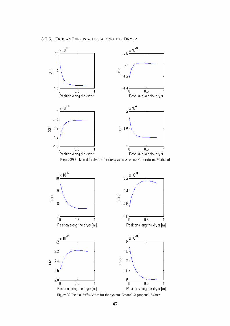
47
8.2.5. FICKIAN DIFFUSIVITIES ALONG THE DRYER
Figure 29 Fickian diffusivities for the system: Acetone, Chloroform, Methanol
Figure 30 Fickian diffusivities for the system: Ethanol, 2-propanol, Water

48
Figure 31 Fickian diffusivities for the system: Water, Ethanol, Ethyl Acetate
Figure 32 Fickian diffusivities for the system: Ethanol, Methylethylketone, Toluene

49
8.2.6. MOLAR EVAPORATION FLUXES ALONG THE DRYER
Figure 33 Molar evaporation fluxes for the system: Acetone, Chloroform, Methanol
Figure 34 Molar evaporation fluxes for the system: Ethanol, 2-propanol, Water

50
Figure 35 Molar evaporation fluxes for the system: Water, Ethanol, Ethyl Acetate
Figure 36 Molar evaporation fluxes for the system: Ethanol, Methylethylketone, Toluene
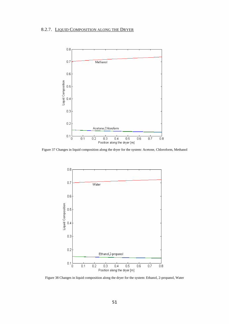
51
8.2.7. LIQUID COMPOSITION ALONG THE DRYER
Figure 37 Changes in liquid composition along the dryer for the system: Acetone, Chloroform, Methanol
Figure 38 Changes in liquid composition along the dryer for the system: Ethanol, 2-propanol, Water

52
Figure 39 Changes in liquid composition along the dryer for the system: Water, Ethanol, Ethyl Acetate
Figure 40 Changes in liquid composition along the dryer for the system: Ethanol, Methylethylketone, Toluene
8.3. PHYSICAL PROPERTIES OF THE COMPONENTS AT 298K
Compound MW b.p.[K] viscosity [cp] Sp.gr.[g/cc] Acetone 58,08 330 0,3075 0,791 Chloroform 119,38 334 1,483 Ethanol 46,07 352 1.074 0,789 Ethyl Acetate 88,11 350 0,426 0,897 Methanol 32,04 338 0,59 0,7918 Methylethylketone 72,11 353 0,43 0,805 2-propanol 60,1 356 1,96 0,786 Toluene 92,14 384 0,590 0,8669 Water 18 373 0.894 1,0
53
8.4. TABLE OF FIGURES
Figure 1 Temperature versus dimensionless position in the particle (left); ethanol composition versus dimensionless position in the particle (right) for the system: Ethanol, 2-propanol, Water. Inlet solid temperature: 298 K, initial composition: [0.15 0.15] ................................................................................................................. 12 Figure 2 Mean temperature of the particle and the outgoing gas for the system: Ethanol, 2-propanol, Water ..... 13 Figure 3 Changes for Fickian diffusivities along the dryer for the system: Ethanol, 2-Propanol, Water at two different initial compositions ................................................................................................................................ 14 Figure 4 Changes of Fickian diffusivities with mean composition for the system: Ethanol, Methylethylketone, Toluene ................................................................................................................................................................. 14 Figure 5 Molar evaporation fluxes for the systems: Ethanol, 2-propanol, Water (a) and Ethanol, Methylethylketone, Toluene (b) ............................................................................................................................ 15 Figure 6 Changes in Fickian diffusivities along the dryer for the system: Ethanol, 2-propanol, Water .............. 16 Figure 7 Changes in Fickian diffusivities along the dryer for the system: Ethanol, Methylethylketone, Toluene 16 Figure 8 Selectivity diagram for the system: Ethanol, 2-Propanol, Water at x0 = [0. 15 0.15] ......................... 17 Figure 9 Selectivity diagram for the system: Ethanol, 2-Propanol, Water at x0 = [0. 33 0.17] ......................... 18 Figure 10 Selectivity diagram for the system: Ethanol, 2-Propanol, Water at x0 = [0. 17 0.33] ......................... 18 Figure 11 Selectivity diagram for the system: Ethanol, 2-Propanol, Water at x0 = [0.33 0.33] .......................... 19 Figure 12 Selectivity diagram for the system: Ethanol, Methylethylketone, Toluene at x0 = [0.33 0.33] ............ 20 Figure 13 Effect of variable diffusion resistance factor (dashed) on selectivity compared to a constant factor (ι=1) (solid) on selectivity for the system Ethanol, 2-propanol, Water ................................................................. 25 Figure 14 Effect of variable diffusion resistance factor (dashed) on selectivity compared to a constant factor (ι=1) (solid) on selectivity for the system: Ethanol, Methylethylketone, Toluene ................................................ 26 Figure 15 Selectivity diagram for the system: Acetone, Chloroform, Methanol at x0 = [0. 15 0.15] ................ 40 Figure 16 Selectivity diagram for the system: Ethanol, 2-propanol, Water at x0 = [0. 15 0.15] ...................... 40 Figure 17 Selectivity diagram for the system: Water, Ethanol, Ethyl Acetate at x0 = [0. 33 0.33] ................... 41 Figure 18 Selectivity diagram for the system: Ethanol , Methylethylketone ,Toluene at x0 = [0. 33 0.33] ...... 41 Figure 19 Mean temperature of the particle and outgoing gas for the system: Acetone, Chloroform, Methanol . 42 Figure 20 Mean temperature of the particle and outgoing gas for the system: Water, Ethanol, Ethyl Acetate ..... 42 Figure 21 Mean temperature of the particle and outgoing gas for the system: Ethanol 2-propanol Water ........... 43 Figure 22 Mean temperature of the particle and outgoing gas for the system: Ethanol, Methylethylketone, Toluene ................................................................................................................................................................. 43 Figure 23 Changes in liquid content along the dryer for the system: Acetone, Chloroform, Methanol ................ 44 Figure 24 Changes in liquid content along the dryer for the system: Ethanol, 2-propanol, Water ....................... 44 Figure 25 Changes in liquid content along the dryer for the system: Water, Ethanol, Ethyl Acetate ................... 45 Figure 26 Changes in liquid content along the dryer for the system: Ethanol, Methylethylketone, Toluene ........ 45 Figure 27 Changes in solid temperature with liquid content for different systems (X0= 0.28 kg/kg dry solid for all systems)................................................................................................................................................................. 46 Figure 28 Changes in solid temperature with liquid content for the system: Ethanol, 2-propanol, Water ............ 46 Figure 29 Fickian diffusivities for the system: Acetone, Chloroform, Methanol .................................................. 47 Figure 30 Fickian diffusivities for the system: Ethanol, 2-propanol, Water ......................................................... 47 Figure 31 Fickian diffusivities for the system: Water, Ethanol, Ethyl Acetate ..................................................... 48 Figure 32 Fickian diffusivities for the system: Ethanol, Methylethylketone, Toluene ......................................... 48 Figure 33 Molar evaporation fluxes for the system: Acetone, Chloroform, Methanol ......................................... 49 Figure 34 Molar evaporation fluxes for the system: Ethanol, 2-propanol, Water ................................................. 49 Figure 35 Molar evaporation fluxes for the system: Water, Ethanol, Ethyl Acetate ............................................. 50 Figure 36 Molar evaporation fluxes for the system: Ethanol, Methylethylketone, Toluene ................................. 50 Figure 37 Changes in liquid composition along the dryer for the system: Acetone, Chloroform, Methanol ........ 51 Figure 38 Changes in liquid composition along the dryer for the system: Ethanol, 2-propanol, Water................ 51 Figure 39 Changes in liquid composition along the dryer for the system: Water, Ethanol, Ethyl Acetate ........... 52 Figure 40 Changes in liquid composition along the dryer for the system: Ethanol, Methylethylketone, Toluene 52