crystal dissolution and precipitation in porous … · crystal dissolution and precipitation in...
TRANSCRIPT
CRYSTAL DISSOLUTION AND PRECIPITATION IN
POROUS MEDIA: PORE SCALE ANALYSIS
C. J. VAN DUIJN AND I. S. POP
Abstract. In this paper we discuss a pore scale model for crys-tal dissolution and precipitation in porous media. We consider firstgeneral domains, for which existence of weak solutions is proven.For the particular case of strips we show that free boundaries oc-cur in the form of dissolution/precipitation fronts. As the ratiobetween the thickness and the length of the strip vanishes we ob-tain the upscaled reactive solute transport model proposed in [12].
1. Introduction
This work is motivated by the crystal dissolution and precipitationmodel introduced in [12]. In that paper the authors present a macro-scopic (core–scale) model, describing transport of ions by fluid flow ina porous medium while undergoing dissolution and precipitation reac-tions. The particularity of the model is in the description of the che-mistry, which involves a multi–valued dissolution rate function. Thisleads to the occurrence of free boundaries (dissolution/precipitationfronts) that were discussed in [17] (equilibrium conditions) and in [3](travelling waves).
If the dissolution rate were a linear term, the model proposed in [12]would fit in the class of porous media transport models with (non–)equilibrium adsorption. Such models received much attention duringthe past years: e.g. see [4], [1], [2], [6], [8], or [13].
All these papers are concerned with the upscaled formulation of thephenomena. A rigorous justification, starting from a well–posed micro-scopic (pore–scale) model and applying a suitable upscaling, has beengiven for important classes of problems. For instance, [9] deals withhomogenization as a method for upscaling and contains an overviewwith particular emphasis on porous media flow including chemical re-actions. In this respect we also mention [10], where the reaction ratesand isotherms are linear (see also [18]), or [11], where nonlinear casesas well as multi–valued interface conditions are analyzed.
In this paper we study the pore–scale analogue of the model proposedin [12]. It builds on Stokes flow in the pores, transport of dissolved ions
1
2 C. J. van Duijn and I. S. Pop
Ω
ΓG
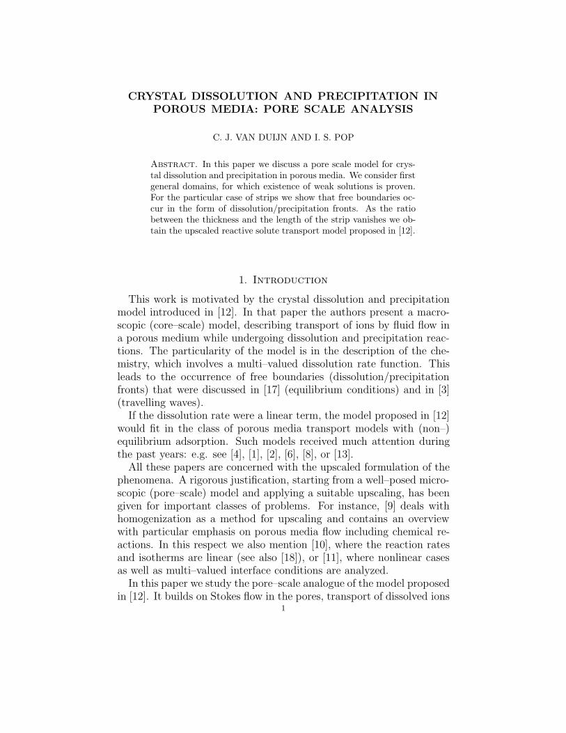
Figure 1. Flow domain with grains.
by convection and diffusion, and dissolution/precipitation reactions onthe surface of the porous skeleton (grains). The latter are described byan ordinary differential equation involving the multi–valued dissolutionrate.
This paper is organized as follows. In the remainder of this sectionwe present the model and recast it in a suitable dimensionless form.In Section 2 we use regularization techniques and a fixed point argu-ment to obtain existence of a weak solution in general domains. Theresults of this section are a first step towards a rigorous justificationof the macroscopic model in [12]. In a forthcoming paper we considerthe second (homogenization) step, including various aspects of solutedispersion.
A particular geometry (a two–dimensional strip) is considered inSection 3. For certain initial and boundary data we show the occurrenceof a dissolution front on the grain surface and we prove some qualitativeproperties. In case of over–saturation a precipitation front occurs withsimilar qualitative behavior. For a better understanding of the upscaledmodel we consider thin strips in Section 4. For vanishing width/lengthratio, we end up with the model discussed in [12], [3] and [4] and thusprovide existence of a suitable weak solution. For completeness we alsoshow uniqueness.
Finally, in Section 5, a numerical example is presented. The resultsare in good agreement with the theory.
1.1. Model equations. We consider a porous medium at the porescale, with Ω ⊂ R
d (d > 1) denoting the void region. This region isoccupied by a fluid in which cations (M1) and anions (M2) are dissolved.The boundary of Ω has an internal part (ΓG), which is the surfacebetween the fluid and the porous matrix (grains), and an external part,which is the outer boundary of the domain.
Crystal dissolution and precipitation in porous media 3
In a precipitation reaction, n particles of M1, and m particles of M2
can precipitate in the form of one particle of a crystalline solid M12,which is attached to the surface of the grains and thus is immobile.The reverse reaction of dissolution is also possible.
We assume that the flow geometry, as well as the fluid density andviscosity (µ > 0, given) are not affected by the reactions and that theflow is described by the Stokes equations relating the fluid velocity ~qand fluid pressure p:
(1.1)µ ∆~q = ∇p,
∇ · ~q = 0,
in Ω.
Along the internal grain boundary we assume a no-slip condition, im-plying
(1.2) ~q = ~0 along ΓG.
Let ci be the volumetric molar concentration of Mi in Ω and c12 thesurface molar concentration of M12 on ΓG. Assuming that both typesof ions have the same diffusion coefficient D > 0 and since crystals areonly present on the grains, mass conservation for Mi gives
(1.3) ∂tci + ∇ · (~qci − D∇ci) = 0, in Ω.
On the interior boundary ΓG the flux of ci is directly related to changesin crystalline concentration c12. Using (1.2) we have
(1.4) ∂tc12 = − 1
nD~ν · ∇c1 = − 1
mD~ν · ∇c2 on ΓG,
where ~ν denotes the normal unit vector pointing into the grains.A second equation for c12 results from a description of the precipi-
tation and dissolution processes. Following the detailed discussion inKnabner et al. [12] (see also [3] and [4]), we have
∂tc12 = rp − rd on ΓG.
Here rp denotes the precipitation rate expressed by
rp = kpr(c1, c2),
where kp is a positive rate constant and r a rate function depending onc1 and c2. A typical example is mass action kinetics leading to
(1.5) r(c1, c2) = cn1c
m2 .
The dissolution rate rd is constant (kd > 0) in the presence of crystal,i.e. for c12 > 0 somewhere on ΓG, and has to be such that in the absenceof crystal the overall rate is zero (for a fluid that is not oversaturated,
4 C. J. van Duijn and I. S. Pop
i.e. r(c1, c2) ≤ kd/kp). To achieve this we introduce the set-valuedexpression
rd(c12) ∈ kdH(c12),
where H denotes the Heaviside graph,
H(u) =
0, if u < 0,[0, 1], if u = 0,1, if u > 0.
If c1 and c2 are such that
r(c1, c2) >kd
kp
somewhere on ΓG,
we have oversaturation and precipitation (∂tc12 > 0) will occur at suchpoints. If the concentrations c1 and c2 are below the solubility product,i.e.
r(c1, c2) <kd
kp
somewhere on ΓG,
while crystal is present, we have ∂tc12 < 0 at such points and dissolutionoccurs. If it also happen that c12 = 0, we set
rd =kp
kdr(c1, c2) < 1,
implying ∂tc12 = 0. Summarizing this discussion we have for the crys-talline solid the equation
(1.6) ∂tc12 ∈ kd
(
kp
kdr(c1, c2) − H(c12)
)
on ΓG.
1.2. Dimensionless form. The unknowns in the model are the fluidvelocity ~q and fluid pressure p, which can be determined without a-priori knowledge of dissolution/precipitation, and the concentrationsc1, c2 and c12. We note that the total negative charge
(1.7) c = mc1 − nc2,
is a conserved quantity with respect to the reactions. Indeed, (1.3) and(1.4) imply
∂tc + ∇ · (~qc − D∇c) = 0 in Ω,
andD~ν · ∇c = 0 on ΓG.
Putting appropriate conditions on c1 and c2 along the outer boundaryof Ω, and thus on c, the total charge in (1.7) can be determined a-priorias well. With respect to the reactions, the essential variables thereforeare c1 (say) and c12. The other concentration (c2) follows directly from(1.7).
Crystal dissolution and precipitation in porous media 5
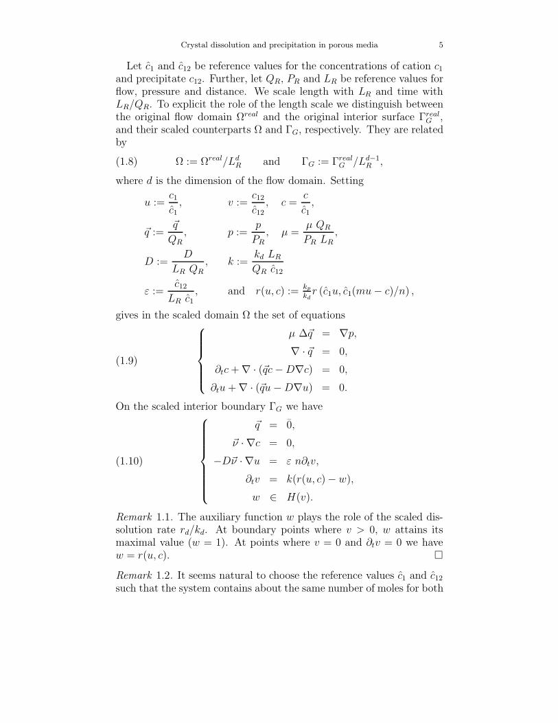
Let c1 and c12 be reference values for the concentrations of cation c1
and precipitate c12. Further, let QR, PR and LR be reference values forflow, pressure and distance. We scale length with LR and time withLR/QR. To explicit the role of the length scale we distinguish betweenthe original flow domain Ωreal and the original interior surface Γreal
G ,and their scaled counterparts Ω and ΓG, respectively. They are relatedby
(1.8) Ω := Ωreal/LdR and ΓG := Γreal
G /Ld−1R ,
where d is the dimension of the flow domain. Setting
u :=c1
c1
, v :=c12
c12
, c =c
c1
,
~q :=~q
QR, p :=
p
PR, µ =
µ QR
PR LR,
D :=D
LR QR, k :=
kd LR
QR c12
ε :=c12
LR c1, and r(u, c) := kp
kdr (c1u, c1(mu − c)/n) ,
gives in the scaled domain Ω the set of equations
(1.9)
µ ∆~q = ∇p,
∇ · ~q = 0,
∂tc + ∇ · (~qc − D∇c) = 0,
∂tu + ∇ · (~qu − D∇u) = 0.
On the scaled interior boundary ΓG we have
(1.10)
~q = 0,
~ν · ∇c = 0,
−D~ν · ∇u = ε n∂tv,
∂tv = k(r(u, c) − w),
w ∈ H(v).
Remark 1.1. The auxiliary function w plays the role of the scaled dis-solution rate rd/kd. At boundary points where v > 0, w attains itsmaximal value (w = 1). At points where v = 0 and ∂tv = 0 we havew = r(u, c).
Remark 1.2. It seems natural to choose the reference values c1 and c12
such that the system contains about the same number of moles for both
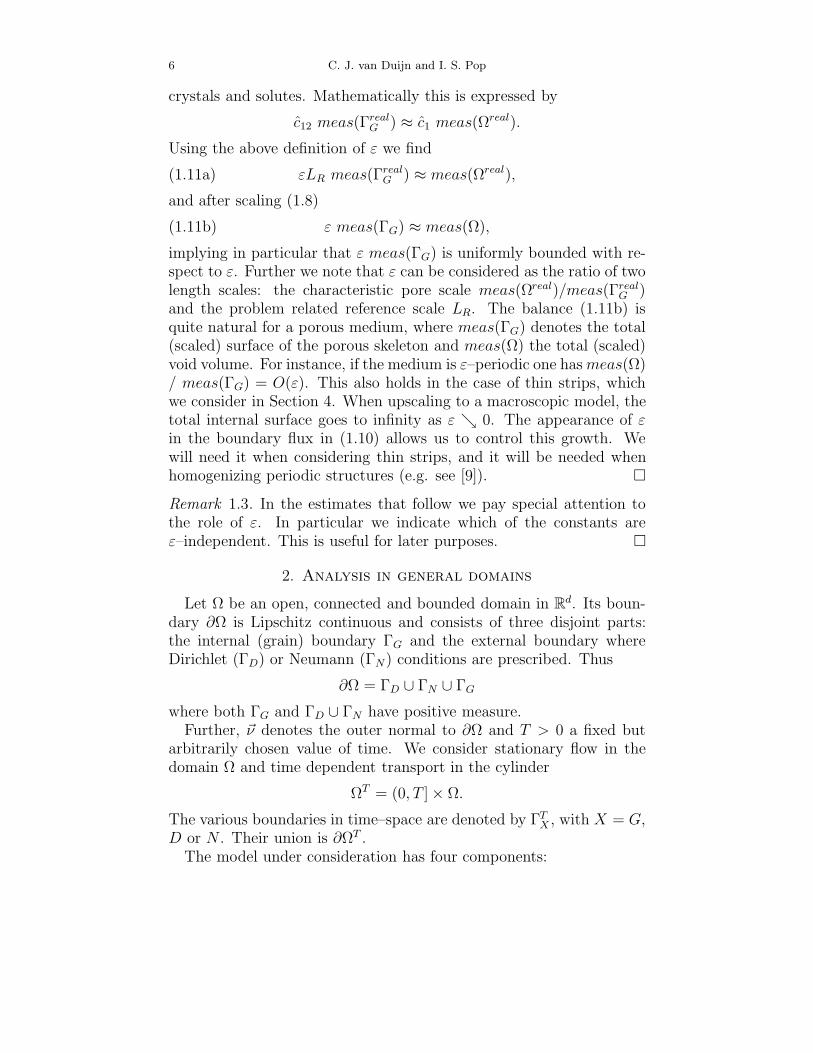
6 C. J. van Duijn and I. S. Pop
crystals and solutes. Mathematically this is expressed by
c12 meas(ΓrealG ) ≈ c1 meas(Ωreal).
Using the above definition of ε we find
(1.11a) εLR meas(ΓrealG ) ≈ meas(Ωreal),
and after scaling (1.8)
(1.11b) ε meas(ΓG) ≈ meas(Ω),
implying in particular that ε meas(ΓG) is uniformly bounded with re-spect to ε. Further we note that ε can be considered as the ratio of twolength scales: the characteristic pore scale meas(Ωreal)/meas(Γreal
G )and the problem related reference scale LR. The balance (1.11b) isquite natural for a porous medium, where meas(ΓG) denotes the total(scaled) surface of the porous skeleton and meas(Ω) the total (scaled)void volume. For instance, if the medium is ε–periodic one has meas(Ω)/ meas(ΓG) = O(ε). This also holds in the case of thin strips, whichwe consider in Section 4. When upscaling to a macroscopic model, thetotal internal surface goes to infinity as ε 0. The appearance of εin the boundary flux in (1.10) allows us to control this growth. Wewill need it when considering thin strips, and it will be needed whenhomogenizing periodic structures (e.g. see [9]).
Remark 1.3. In the estimates that follow we pay special attention tothe role of ε. In particular we indicate which of the constants areε–independent. This is useful for later purposes.
2. Analysis in general domains
Let Ω be an open, connected and bounded domain in Rd. Its boun-
dary ∂Ω is Lipschitz continuous and consists of three disjoint parts:the internal (grain) boundary ΓG and the external boundary whereDirichlet (ΓD) or Neumann (ΓN) conditions are prescribed. Thus
∂Ω = ΓD ∪ ΓN ∪ ΓG
where both ΓG and ΓD ∪ ΓN have positive measure.Further, ~ν denotes the outer normal to ∂Ω and T > 0 a fixed but
arbitrarily chosen value of time. We consider stationary flow in thedomain Ω and time dependent transport in the cylinder
ΩT = (0, T ] × Ω.
The various boundaries in time–space are denoted by ΓTX , with X = G,
D or N . Their union is ∂ΩT .The model under consideration has four components:
Crystal dissolution and precipitation in porous media 7
Fluid flow:
(2.1)
µ ∆~q = ∇p, in Ω,∇ · ~q = 0, in Ω,
~q = ~0, on ΓG,~q = ~qD, on ΓD,
~ν · ~q = 0, on ΓN ;
Total charge transport:
(2.2)
∂tc + ∇ · (~qc − D∇c) = 0, in ΩT ,~ν · ∇c = 0, on ΓT
G,c = cD, on ΓT
D,~ν · ∇c = 0, on ΓT
N ,c = cI , in Ω, for t = 0;
Ion transport:
(2.3)
∂tu + ∇ · (~qu − D∇u) = 0, in ΩT ,−D~ν · ∇u = εn∂tv, on ΓT
G,u = uD, on ΓT
D,~ν · ∇u = 0, on ΓT
N ,u = uI , in Ω, for t = 0,
Precipitation/dissolution:
(2.4)
∂tv = k(r(u, c)− w), on ΓTG,
w ∈ H(v), on ΓTG,
v = vI , on ΓG, for t = 0.
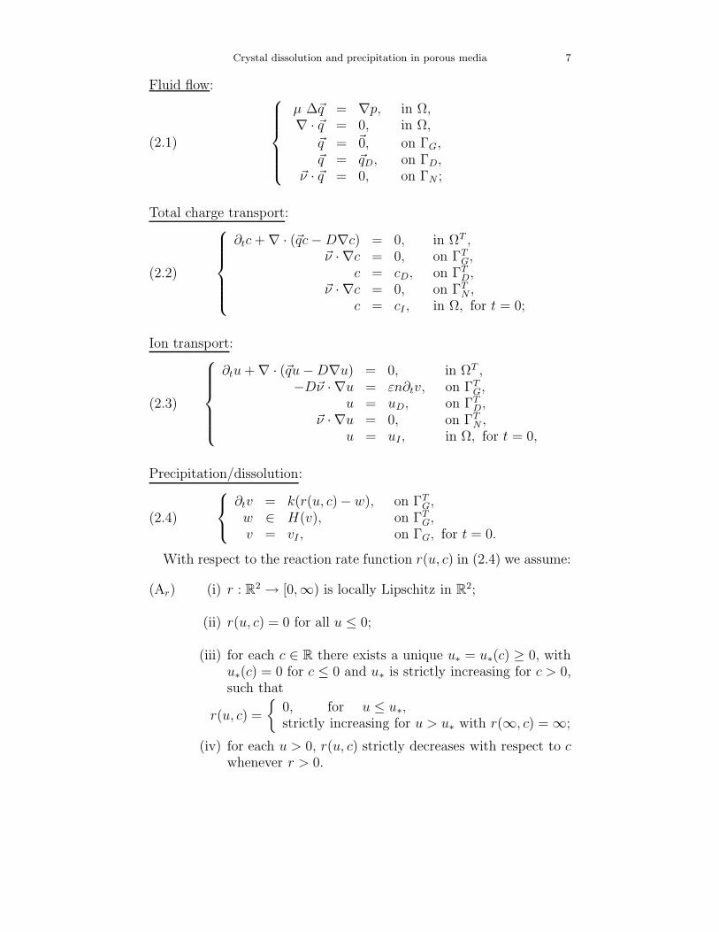
With respect to the reaction rate function r(u, c) in (2.4) we assume:
(Ar) (i) r : R2 → [0,∞) is locally Lipschitz in R
2;
(ii) r(u, c) = 0 for all u ≤ 0;
(iii) for each c ∈ R there exists a unique u∗ = u∗(c) ≥ 0, withu∗(c) = 0 for c ≤ 0 and u∗ is strictly increasing for c > 0,such that
r(u, c) =
0, for u ≤ u∗,strictly increasing for u > u∗ with r(∞, c) = ∞;
(iv) for each u > 0, r(u, c) strictly decreases with respect to cwhenever r > 0.
8 C. J. van Duijn and I. S. Pop
u
c
*
r > 0
r = 0
*u (c)
1
u (c)**u (c) u
r(u, c)
c < 0c > 0
Figure 2. Typical examples for u∗ (left) and r (right).
Example. Assuming mass action kinetics (1.5), replacing ci by itsnon–negative part [ci]+ and using (1.7), we obtain
(2.5) r(u, c) = K ([u]+)m
([
mu − c
n
]
+
)n
,
for some K > 0. Here u∗(c) = [c]+m
. This example is sketched in Figure2.
Concerning the data we assume:
(AD) Boundary and initial data are bounded; for u and v these arealso non-negative; all boundary data are constant in time andtraces of H1 – functions.
Remark 2.1. Since u and v model concentrations, the sign assumptionsand boundedness are not restrictive for applications. We consider hereconstant in time boundary data to avoid non essential technical details.
Remark 2.2. To express u = uD on ΓD, for instance, we use below thewell–known notation
u ∈ uD + H10,ΓD
(Ω),
where uD is the H1–extension of the Dirichlet boundary condition.
2.1. Results concerning flow and total charge. Since chemistrydoes not affect flow, the Stokes system (2.1) can be treated indepen-dently from the ion transport. We follow [20] and obtain the existence
Crystal dissolution and precipitation in porous media 9
of a unique weak solution ~q ∈ ~qD +(
H10,ΓD
(Ω))d
satisfying ∇ · ~q = 0 in
Ω, ~q|ΓG= ~0 and
(2.6) (∇~q,∇~Ψ) = 0,
for all ~Ψ ∈(
H10,ΓD
(Ω))d
with ~Ψ|ΓG= ~0 and ∇ · ~Ψ = 0 in Ω. Having
~q ∈ (H1(Ω))d, the fluid pressure p is defined in L2(Ω) uniquely up to a
constant.Since the data ~qD is bounded on ΓD we have:
Lemma 2.3. Let ‖~qD‖∞,ΓD= Mq. Then ‖~q‖∞,Ω = Mq.
Proof. Testing with ~Ψ = [~q ± Mq]+ in (2.6) yields the result.
With ~q being defined in Ω we consider the linear transport of thetotal charge c. Let
C := c ∈ cD + L2((0, T ); H10,ΓD
(Ω)) : ∂tc ∈ L2((0, T ); H−1(Ω)).As in chapters 3.3 and 3.4 of [14], or chapter 23 of [22] we find a uniqueweak solution c ∈ C of (2.2) satisfying c(0) = cI in Ω and
(2.7) (∂tc, ϕ)ΩT + D(∇c,∇ϕ)ΩT − (~qc,∇ϕ)ΩT = 0,
for all ϕ ∈ L2((0, T ); H10,ΓD
(Ω)).Furthermore, the boundedness of the data extends to c:
Lemma 2.4. Let Mc := max‖cD‖∞,ΓD, ‖cI‖∞,Ω. Then ‖c‖∞,ΩT =
Mc.
Remark 2.5. Suppose ΓD has measure 0. Then there are no prescribedvalues for the total charge on the boundary. With χ(0,t) denoting thecharacteristic function of the interval (0, t), ϕ ≡ χ(0,t) is an admissibletest function in (2.7) for any t ≤ T . Thus we see that the total chargeis a conserved quantity; i.e.
∫
Ω
c(t, x)dx =
∫
Ω
cI(x)dx.
2.2. Analysis of crystal dissolution and precipitation. The che-mical process is essentially modelled by (2.4) and the flux in (2.3). Themain difficulty is the occurrence of the multi–valued function describingthe dissolution. Let
U := u ∈ uD + L2((0, T ); H10,ΓD
(Ω)) : ∂tu ∈ L2((0, T ); H−1(Ω)),V := v ∈ H1((0, T ); L2(ΓG)),W := w ∈ L∞(ΓT
G), : 0 ≤ w ≤ 1.
10 C. J. van Duijn and I. S. Pop
Definition 2.1. A triple (u, v, w) ∈ U×V×W is called a weak solutionof (2.3) and (2.4) if (u(0), v(0)) = (uI , vI) and if
(2.8) (∂tu, ϕ)ΩT + D(∇u,∇ϕ)ΩT − (~qu,∇ϕ)ΩT = −εn(∂tv, ϕ)ΓTG,
(2.9)(∂tv, θ)ΓT
G= k(r(u, c) − w, θ)ΓT
G,
w ∈ H(v) a.e. in ΓTG,
for all (ϕ, θ) ∈ L2((0, T ); H10,ΓD
(Ω)) × L2(ΓTG).
2.2.1. L∞–bounds. In view of (AD) we expect u and v to be non–negative and bounded. These properties are shown in the followinglemmas.
Lemma 2.6. The concentrations u and v are non–negative a.e. in ΩT ,respectively ΓT
G.
Proof. Since u(t) ∈ uD + H10,ΓD
(Ω) for almost every 0 < t < T and
since uD is positive, we have [u]− ∈ L2((0, T ); H10,ΓD
(Ω)), where [u]−denotes the negative part of u. For any 0 < t < T , we test (2.8) withϕ := χ(0,t)[u]− giving
12‖[u(t)]−‖2
Ω + D‖∇[u]−‖2Ωt − (~qu,∇[u]−)Ωt
= 12‖[uI ]−‖2
Ω − εn(∂tv, [u]−)ΓtG.
The convection term in this expression vanishes. This follows from
(~qu,∇[u]−)Ωt = 12(~q,∇[u]2−)Ωt =
12(~ν · ~q, [u]2−)Γt
N∪ΓtD
+ 12(~ν · ~q, [u]2−)Γt
G− 1
2([u]2−,∇ · ~q)Ωt
and the boundary conditions on ∂Ω, together with ∇ · ~q = 0 in Ω.Moreover, since uI ≥ 0 in Ω, the first term on the right vanishes as
well. Finally, because [u]− ≤ 0 a.e. and belongs to L2((0, T ); H10,ΓD
(Ω)),
its trace [u|ΓG]− is a non-positive L2(ΓT
G) function. Testing with θ :=χ(0,t)[u|ΓG
]− in (2.9) gives
(∂tv, [u]−)ΓtG
= k(r(u, c) − w, [u]−)ΓtG
= −k(w, [u]−)ΓtG≥ 0,
where we have used (A1) and the positivity of w.Combining these observations leaves us with
1
2‖[u(t)]−‖2
Ω + D‖∇[u]−‖2Ωt ≤ 0,
showing that u(t) is non–negative for all t ≥ 0.Testing (2.9) with θ := [v]− gives the same result for v.
Crystal dissolution and precipitation in porous media 11
Assumption (Ar) implies that for each c ∈ R a unique u∗(c) > 0exists such that
r(u∗(c), c) = 1.
The function u∗ : R → R is clearly continuous and non–decreasing.With Mc from Lemma 2.4 we define
Mu := max ‖uI‖∞,Ω, ‖uD‖∞,ΓD, u∗(Mc) .
Lemma 2.7. The concentration u satisfies u ≤ Mu a.e. in ΩT .
Proof. For any t ∈ (0, T ] we test (2.8) with ϕ := χ(0,t)[u − Mu]+ ∈L2((0, T ); H1
0,ΓD(Ω)) and obtain
12‖[u(t) − Mu]+‖2
Ω + D‖∇[u − Mu]+‖2Ωt − (~qu,∇[u − Mu]+)Ωt
= 12‖[uI − Mu]+‖2
Ω − εn(∂tv, [u − Mu]+)ΓtG.
Arguing as in the proof of Lemma 2.6 we first observe that the con-vection term and the first term on the right vanish. To handle thereaction term we note that, if u ≥ Mu,
r(u, c) ≥ r(Mu, c) ≥ r(Mu, Mc) ≥ r(u∗(Mc), Mc) = 1.
Together with the positivity of [u − Mu]+ this implies
(∂tv, [u − Mu]+)ΓtG
= k(r(u, c) − w, [u − Mu]+)ΓtG
≥ k(1 − w, [u − Mu]+)ΓtG≥ 0.
Therefore we are left with1
2‖[u(t) − Mu]+‖2
Ω + D‖∇[u − Mu]+‖2Ωt ≤ 0,
implying u ≤ Mu a.e. in ΩT .
As an immediate consequence we have for v:
Corollary 2.8. Let Mv := max‖vI‖∞,Ω, 1. Then
(2.10) v(t, ·) ≤ Mv eCt a.e. in ΓG
for all 0 ≤ t ≤ T . Here C := kr(Mu,−Mc)/Mv.
Remark 2.9. On the compact set (u, c) : 0 ≤ u ≤ Mu, |c| ≤ Mcthe reaction rate function r(u, c) has the Lipschitz constant Lr. Sincer(u, c) = 0 for u ≤ 0 we obtain the bounds
0 ≤ r(u, c) ≤ Lru ≤ LrMu, a.e. in ΓTG.
If there are no prescribed boundary values for the ion concentration,we end up with the following mass balance:
12 C. J. van Duijn and I. S. Pop
Proposition 2.10. Let meas(ΓD) = 0. Then∫
Ω
u(t, x)dx + εn
∫
ΓG
v(t, s)ds =
∫
Ω
uI(x)dx + εn
∫
ΓG
vI(s)ds
for all 0 ≤ t ≤ T .
Proof. Testing (2.8) with ϕ = χ(0,t) ∈ L2((0, T ); H1(Ω)) yields directlythe result.
2.2.2. Existence of a solution. To prove existence of a weak solution wereplace the Heaviside graph by the Lipschitz approximation (δ beingpositive and small)
Hδ(v) :=
0, if v < 0,v/δ, if v ∈ (0, δ),1, if v > δ,
and consider the regularized problem:
Problem Pδ: Find (u, v) ∈ U × V, such that (u(0), v(0)) = (uI , vI)and
(2.11) (∂tu, ϕ)ΩT + D(∇u,∇ϕ)ΩT − (~qu,∇ϕ)ΩT = −εn(∂tv, ϕ)ΓTG,
(2.12) (∂tv, θ)ΓTG
= k(r(u, c)− Hδ(v), θ)ΓTG,
for all (ϕ, θ) ∈ L2((0, T ); H10,ΓD
(Ω)) × L2(ΓTG).
We borrow some ideas of [1] to prove existence for (Pδ) with fixedδ > 0. With Mu and Mv defined in Section 2.2.1, we consider the closedand convex sets
KU := u ∈ uD + L2((0, T ); H10,ΓD
(Ω)) : 0 ≤ u ≤ Mu a.e. in ΩT ,KV := v ∈ V : 0 ≤ v ≤ Mve
CT a.e. in ΓTG.
For arbitrary u ∈ KU we consider equation (2.12) subject to v(0) = vI .Since Hδ is Lipschitz there exists a unique solution v ∈ KV . Further,given v ∈ KV , equation (2.11) with u(0) = uI has a unique solutionT u ∈ KU (see e.g. [14], chapter 5.7). In this way u ∈ KU generates aunique T u ∈ KU , where the operator
(2.13) T : KU → KU
is defined by successively solving (2.12) and (2.11). Clearly, a fixedpoint of T defines a solution of (Pδ).
We start with some a-priori estimates.
Crystal dissolution and precipitation in porous media 13
Lemma 2.11. There exists C > 0 such that
‖T u(t)‖2Ω + ‖∇T u‖2
Ωt + ‖∂tT u‖2L2((0,t);H−1(Ω)) ≤ C
for all 0 ≤ t ≤ T and for all u ∈ KU . Here C does not depend on δ.
Proof. Fix an arbitrary t ∈ (0, T ] and test (2.11) with ϕ := χ(0,t)(T u−uD). Using (2.12) this gives
12
∫ t
0∂s‖T u(s) − uD‖2
Ωds + D‖∇T u‖2Ωt
= D∫ t
0(∇T u(s),∇uD)Ωds +
∫ t
0(~qT u(s),∇(T u(s) − uD))Ωds
+εnk(Hδ(v), T u − uD)ΓtG− εnk(r(u, c), T u − uD)Γt
G.
This expression contains six terms. Denoting them by I1, . . . , I6 weestimate
I1 = 12(‖T u(t) − uD‖2
Ω − ‖uI − uD‖2Ω)
≥ 14‖T u(t)‖2
Ω − 12(‖uD‖2
Ω + ‖uI − uD‖2Ω)
=: 14‖T u(t)‖2
Ω − CI1.
The term I2 needs no further estimate. For I3 we have
|I3| ≤D
4‖∇T u‖2
Ωt + Dt‖∇uD‖2Ω ≤ D
4‖∇T u‖2
Ωt + CI2,
with CI2 chosen sufficiently large so that it is time independent.To estimate I4 we write
|I4| ≤∣
∣
∣
∫ t
0(~q(T u(s) − uD),∇(T u(s) − uD))Ωds
∣
∣
∣
+∫ t
0|(~quD,∇T u(s))Ω| ds +
∫ t
0|(~quD,∇uD)Ω| ds.
The first term on the right vanishes because ∇·~q = 0 in Ω and T u = uD
on ΓD. The last two terms we estimate with Lemma 2.3 to obtain
|I4| ≤ D4‖∇T u‖2
Ωt +tM2
q
D‖uD‖2
Ω + tMq
2‖uD‖2
H1(Ω)
=: D4‖∇T u‖2
Ωt + CI4.
In I5 the L∞–bounds of u gives
(2.14) |I5| ≤ εnkMumeas(ΓG)t + εnkt
∫
ΓG
|uD| ≤ CI5,
for CI5 sufficiently large. Finally, since both T u and r(u, c) are non–negative, Remark 2.9 implies
(2.15) |I6| ≤ εnkLrMut
∫
ΓG
|uD| ≤ CI6,
again for CI6 large enough. Combining these estimates gives the firsttwo inequalities of the Lemma.
14 C. J. van Duijn and I. S. Pop
To prove the last part of the lemma we notice that
(2.16)|(∂tT u(t), ϕ)Ω| ≤ (D‖∇T u(t)‖Ω + Mq‖T u‖Ω) ‖∇ϕ‖Ω
+εnk∣
∣(r(u(t), c) − Hδ(v(t)), ϕ)ΓG
∣
∣ ,
for all ϕ ∈ H10,ΓD
(Ω) and almost all t > 0. Using the L∞–bounds for u,c and Hδ, and the trace inequality
‖ϕ‖ΓG≤ C(Ω)‖ϕ‖H1(Ω),
we obtain
|(∂tT u(t), ϕ)Ω| ≤ D‖∇T u(t)‖Ω + Mq‖T u‖Ω
+εnk(1 + LrMu)C(Ω) ‖ϕ‖H1(Ω).
Because ϕ ∈ H10,ΓD
(Ω) is arbitrary, it follows that
‖∂tT u(t)‖H−1(Ω) ≤ D‖∇T u(t)‖Ω + Mq‖T u‖Ω + εnk(1 + LrMu)C(Ω))
for almost every t > 0. Using the first part of the lemma (provenbefore) gives the desired estimate.
Remark 2.12. If (1.11b) holds, the constants in (2.14) and (2.15) canbe chosen independently of ε. Further, if the domain is ε–periodicwe use Lemma 3 of [10], saying that there exists a constant C > 0,independent of ε, such that
ε
∫
ΓG
|ϕ| ≤ ε meas1/2(ΓG) ‖ϕ‖ΓG≤ C
(
‖ϕ‖2Ω + ε2‖∇ϕ‖2
Ω
)1/2
for all ϕ ∈ H1(Ω). Using this to estimate the boundary term in (2.16)yields a constant C in Lemma 2.11 which does not depend on ε aswell.
By similar arguments we obtain a–priori estimates for v.
Lemma 2.13. Given u ∈ KU let v denote the solution of (2.12) subjectto v(0) = vI . Then there exists C > 0 such that
‖v(t)‖2ΓG
+ ‖∂tv‖2ΓT
G≤ C,
for all t ∈ (0, T ] and for all u ∈ KU . Here C > 0 does not depend onδ.
Proof. The first part results from Corollary 2.8. The proof of the secondpart is similar to the last part of the proof of Lemma 2.11.
Remark 2.14. Assuming again (1.11b), one directly deduces that theconstant C in Lemma 2.13 is in fact C/ε, where C does not depend onε.
Crystal dissolution and precipitation in porous media 15
To show existence of a fixed point for T we use a contraction argu-ment. To this end we consider any u1, u2 ∈ KU , with v1, v2 ∈ KV thecorresponding solutions of (2.12). Further we introduce the notation
N(u, t) := ‖u‖2L2((0,t); H1(Ω)) = ‖u‖2
Ωt + ‖∇u‖2Ωt.
By the trace inequality we have
(2.17) ‖u‖2Γt
G≤ C(Ω)N(u, t), for all u ∈ L2((0, T ); H1
0,ΓD(Ω)).
The goal is to estimate T u := T u1 −T u2 in terms of u := u1 −u2. Wefirst consider the reaction equation.
Lemma 2.15. Let v := v1 − v2. For any t ∈ (0, T ] we have
‖v‖2Γt
G≤ C1(e
t − 1) N(u, t),
‖∂tv‖2Γt
G≤ C2(t)N(u, t),
with C1 = C(Ω)k2L2r and C2(t) = 2C1(1 + (k/δ)2 (et − 1)). Here Lr is
the Lipschitz constant given in Remark 2.9 and C(Ω) is the constantfrom (2.17).
Proof. Writing (2.12) for the difference v = v1 − v2 and testing withθ = χ(0,t)v for arbitrary 0 < t ≤ T gives
12∂t‖v‖2
ΓG= k(r(u1, c) − r(u2, c) − (Hδ(v1) − Hδ(v2)), v)ΓG
≤ k(r(u1, c) − r(u2, c), v)ΓG
by the monotonicity of Hδ. Since r is Lipschitz we have
‖v(t)‖2ΓG
≤ 2kLr(|u|, |v|)ΓtG≤ k2L2
r‖u‖2Γt
G+ ‖v‖2
ΓtG
for all 0 ≤ t ≤ T . In this expression we substitute (2.17). Directintegration gives the first estimate.
To obtain the second one we test with θ = χ(0,t)∂tv. This gives forall 0 ≤ t ≤ T
‖∂tv‖2Γt
G= k(r(u1, c) − r(u2, c) − (Hδ(v1) − Hδ(v2)), ∂tv)Γt
G
≤ kLr(|u|, |∂tv|)ΓtG
+ kδ(|v|, |∂tv|)Γt
G
≤ k2L2r‖u‖2
ΓtG
+ k2
δ2 ‖v‖2Γt
G+ 1
2‖∂tv‖2
ΓtG,
implying the desired estimate.
Next we estimate T u = T u1 − T u2.
16 C. J. van Duijn and I. S. Pop
Lemma 2.16. For all t ∈ (0, T ] and µ > 0
‖T u‖2Ωt ≤ µ3A(t)
µC3+C4
(
et (µC3+C4)
µ2 − 1
)
N(u, t),
‖∇T u‖2Ωt ≤ µA(t)
De
t (µC3+C4)
µ2 N(u, t),
where A(t) = ε2n2C2(t)/2, with C2(t) from Lemma 2.15, and where C3
and C4 are positive constants depending on Ω and D but not on theregularization parameter δ.
Proof. Writing (2.11) for the difference T u = T u1 − T u2 and testingwith θ = χ(0,t)T u for arbitrary 0 < t ≤ T gives
1
2‖T u(t)‖2
Ω + D‖∇T u‖2Ωt = −εn(∂tv, T u)Γt
G.
Note that the convection term has disappeared. This is a consequenceof (2.1) and the boundary conditions. Hence, for any µ > 0
12‖T u(t)‖2
Ω + D‖∇T u‖2Ωt ≤ µ ε2n2
4‖∂tv‖2
ΓtG
+ 1µ‖T u‖2
ΓtG
≤ µ ε2n2
4C2(t)N(u, t) + 1
µ‖T u‖2
ΓtG
by Lemma 2.15.Following the proof of the trace theorem, e.g. see [5], chapter 5.5 or
[7], Theorem 1.5.1.10, there exists positive constants C3 and C4 suchthat
(2.18) ‖ϕ‖2ΓG
≤ C3‖ϕ‖2Ω + +C4‖ϕ‖Ω‖∇ϕ‖Ω
for all ϕ ∈ H10,ΓD
(Ω). Applying this inequality to ϕ = T u yields
(2.19)‖T u(t)‖2
Ω + 2D‖∇T u‖2Ωt
≤ µA(t)N(u, t) +(
C3
µ+ C4
µ2
)
‖T u‖2Ωt + D‖∇T u‖2
Ωt ,
for an appropriately redefined C4. Disregarding the gradient terms inthis inequality, integrating the result with respect to t and using themonotonicity of A(·) and N(u, ·), yields the first estimate of the lemma.Using it in (2.19) gives the gradient estimate.
A direct consequence of Lemma 2.16 is
Corollary 2.17. For all t ∈ (0, T ] and µ > 0, and for all u1, u2 ∈ KU
N(T u1 − T u2, t)
≤ µA(t)[
µ2(et(C3µ+C4)/µ2−1)
C3µ+C4+ et(C3µ+C4)/µ2
D
]
N(u1 − u2, t).
Crystal dissolution and precipitation in porous media 17
The constants C1, C3 and C4 in the estimates do not depend on theinitial data. Further, taking T as an upper bound for t, C2(t) and thusA(t) can be bounded from above by a constant independent of t andthe initial data. Choosing now t = µ2, the estimate in Corollary (2.17)can be written as
(2.20) N(T u1 − T u2, µ2) ≤ µCN(u1 − u2, µ
2),
where the constant C does not depend on the initial data and µ. Withµ small enough (but fixed) we thus have shown that T is a contractionon the closed set u ∈ uD + L2((0, µ2); H1
0,ΓD(Ω)) : 0 ≤ u ≤ Mu,
and that it has a fixed point u in this set. By Lemma 2.11, u ∈H1((0, µ2); H−1(Ω)) and satisfies its a-priori estimates. In particularu ∈ C([0, µ2]; L2(Ω)) with 0 ≤ u(µ2) ≤ Mu. So u(µ2) can be used asinitial condition for extending the time interval of existence. Since µdoes not depend on the initial data, we have obtained a fixed point ofT for the arbitrary time interval (0, T ):
Lemma 2.18. The fixed point u of T belongs to KU∩H1((0, T ); H−1(Ω)),and satisfies
‖u(t)‖2Ω + ‖∇u‖2
Ωt + ‖∂tu‖2L2((0,t);H−1(Ω)) ≤ C,
for all t > 0. Here C > 0 does not depend on δ.
Starting with an arbitrary u0 ∈ KU a sequence ukk≥1 ⊂ KU ∩H1((0, T ); H−1(Ω)) is constructed by the iterations uk = T uk−1, k ≥ 1.This sequence converges strongly to the fixed point u in L2((0, T ); H1
0,ΓD(Ω))
and is uniformly bounded in H1((0, T ); H−1(Ω)). Hence it has a weaklyconvergent subsequence uknn≥0 with u ∈ H1((0, T ); H−1(Ω)) as theweak limit. By construction, all ukn satisfy the initial and boundarydata and(2.21)
(∂tukn, ϕ)ΩT + D(∇ukn,∇ϕ)ΩT − (~qukn,∇ϕ)ΩT = −εn(∂tv
kn, ϕ)ΓTG,
for all ϕ ∈ L2((0, T ); H10,ΓD
(Ω). Here vkn solves
(2.22) (∂tvkn, θ)ΓT
G= k(r(ukn−1, c) − Hδ(v
kn), θ)ΓTG,
for all θ ∈ L2(ΓTG), with vI as initial data. By Lemma 2.15, the sequence
vknn≥0 converges strongly in H1((0, T ); L2(ΓG)) to a limit v. Sincer and Hδ are continuous we can pass to the limit in (2.21) and (2.22)and obtain that (u, v) is a solution of the regularized problem Pδ. Wesummarize:
18 C. J. van Duijn and I. S. Pop
Theorem 2.19. For each δ > 0, Problem Pδ has a solution (uδ, vδ) ∈U × V that satisfies
0 ≤ uδ ≤ Mu, 0 ≤ vδ ≤ MveCT a.e. in ΩT , respectively ΓT
G,
and‖uδ(t)‖2
Ω + ‖∇uδ‖2Ωt + ‖∂tuδ‖2
L2((0,t);H−1(Ω))
+ε‖vδ(t)‖2ΓG
+ ε‖∂tvδ‖2Γt
G≤ C,
for all t > 0. Here C > 0 does not depend on δ. If in addition theconditions of Remark 2.12 hold, then C does not depend on ε as well.
Remark 2.20. Since both r and Hδ are Lipschitz, Problem Pδ has aunique solution. To see this we assume that both (u1, v1) and (u2, v2)solve Pδ. With u := u1 − u2 and v := v1 − v2, we follow the proof ofLemma 2.15 and find
‖v‖2Γt
G≤ k2L2
r(et − 1)‖u‖2
ΓtG
for all 0 ≤ t ≤ T . Since r is monotone, (2.11) and (2.12) imply
1
2‖u(t)‖2
Ω + D‖∇u‖2Ωt ≤ C‖u‖2
ΓtG,
where C = εnk2Lr
δ
√et − 1. Using (2.18) we obtain
12‖u(t)‖2
Ω + D‖∇u‖2Ωt ≤ C (C3‖u‖2
Ωt + C4‖u‖Ωt‖∇u‖Ωt)
≤ C[(
C3 +C2
4
4µ
)
‖u‖2Ωt + µ‖∇u‖Ωt
]
.
Taking µ = D/C and using Gronwall’s lemma gives u = 0 and hencev = 0.
Finally we send δ 0. Theorem 2.19 provides an approximatesolution for each δ > 0 and the necessary uniform estimates. Letwδ ∈ L∞(ΓT
G) be defined by
wδ(t, x) = Hδ(vδ(t, x)) a.e. in ΓTG.
Compactness arguments give the existence of a triple (u, v, w) ∈ U ×V × L∞(ΓT
G) and a subsequence δ 0, such that
a) uδ → u weakly in L2((0, T ); H10,ΓD
(Ω)),b) ∂tuδ → ∂tu weakly in L2((0, T ); H−1(Ω)),c) vδ → v weakly in L2((0, T ); L2(ΓG)),d) ∂tvδ → ∂tv weakly in L2(ΓT
G),e) wδ → w weakly–star in L∞(ΓT
G).
We now state the main result of this section.
Crystal dissolution and precipitation in porous media 19
Theorem 2.21. The triple (u, v, w) is a weak solution of (2.3), (2.4)in the sense of Definition 2.1. It satisfies
0 ≤ u ≤ Mu, a.e. in ΩT
0 ≤ v ≤ MveCT , 0 ≤ w ≤ 1 a.e. in ΓT
G
‖u(t)‖2Ω + ‖∇u‖2
Ωt + ‖∂tu‖2L2((0,t);H−1(Ω))
+ε‖vδ(t)‖2ΓG
+ ε‖∂tvδ‖2Γt
G≤ C,
for all 0 ≤ t ≤ T , where C is the constant from Theorem 2.19. More-over,
w = r(u, c) a.e. in v = 0 ∩ ΓTG.
Proof. By the weak convergence, all bounds are inherited from Theo-rem 2.19. Furthermore, it is immediate that u and v satisfy equation(2.8). Only the reaction equation needs additional attention. We firstconsider the behavior of uδ on ΓT
G. By the a–priori estimates and byLemma 9 and Corollary 4 of [19], we have
uδ → u strongly in C([0, T ]; H−s(Ω)) ∩ L2(0, T ; Hs(Ω))
for any s ∈ (0, 1). Then the trace theorem, see Satz 8.7 of [21], gives
uδ → u strongly in L2(0, T ; Hs−1/2(ΓG))
and in particular
uδ → u strongly in L2(ΓTG).
Since r is Lipschitz, this yields
r(uδ, c) → r(u, c) strongly in L2(ΓTG)
and pointwisely a.e. in ΓTG. This observation and the weak–star con-
vergence of wδ implies that u, v and w satisfy (2.91). It remains toshow that (2.92) holds. This would be trivial in the case of pointwisevδ convergence. However we only have weak convergence. To resolvethis we use the regularized reaction equation (2.12). First introduce
v(t, x) := lim infδ0
vδ(t, x) ≥ 0 a.e. in ΓTG,
and decompose ΓTG = S1 ∪ S2, where (in the almost everywhere sense)
S1 = v > 0 and S2 = v = 0,We show that v > 0 and w = 1 in S1, while v = 0 and w = r(u) ∈ [0, 1]in S2.
20 C. J. van Duijn and I. S. Pop
z
L x0
Ω
H=1
Γ
symmetry
ΓG
ΓN
ΓDD
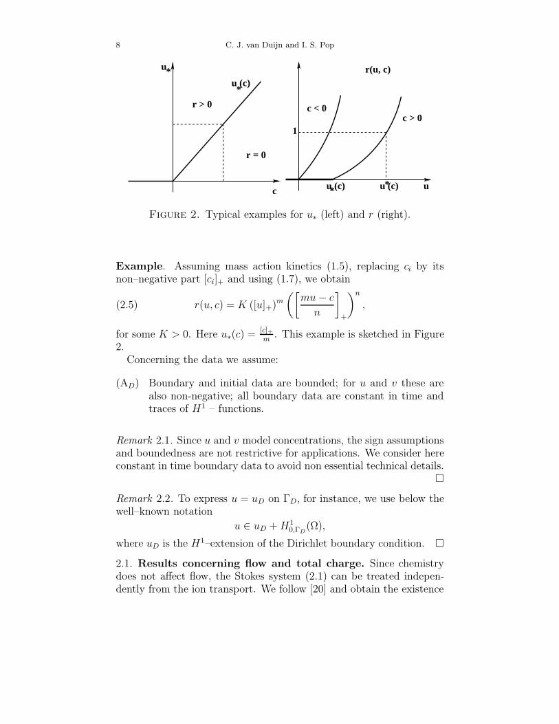
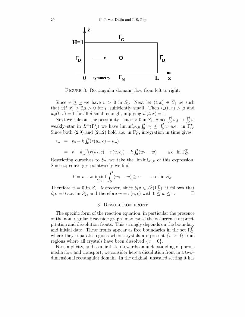
Figure 3. Rectangular domain, flow from left to right.
Since v ≥ v we have v > 0 in S1. Next let (t, x) ∈ S1 be suchthat v(t, x) > 2µ > 0 for µ sufficiently small. Then vδ(t, x) > µ andwδ(t, x) = 1 for all δ small enough, implying w(t, x) = 1.
Next we rule out the possibility that v > 0 in S2. Since∫ t
0wδ →
∫ t
0w
weakly–star in L∞(ΓTG) we have lim infδ0
∫ t
0wδ ≤
∫ t
0w a.e. in ΓT
G.
Since both (2.9) and (2.12) hold a.e. in ΓTG, integration in time gives
vδ = v0 + k∫ t
0(r(uδ, c) − wδ)
= v + k∫ t
0(r(uδ, c) − r(u, c)) − k
∫ t
0(wδ − w) a.e. in ΓT
G.
Restricting ourselves to S2, we take the lim infδ0 of this expression.Since uδ converges pointwisely we find
0 = v − k lim infδ0
∫ t
0
(wδ − w) ≥ v a.e. in S2.
Therefore v = 0 in S2. Moreover, since ∂tv ∈ L2(ΓTG), it follows that
∂tv = 0 a.e. in S2, and therefore w = r(u, c) with 0 ≤ w ≤ 1.
3. Dissolution front
The specific form of the reaction equation, in particular the presenceof the non–regular Heaviside graph, may cause the occurrence of preci-pitation and dissolution fronts. This strongly depends on the boundaryand initial data. These fronts appear as free boundaries in the set ΓT
G,where they separate regions where crystals are present v > 0 fromregions where all crystals have been dissolved v = 0.
For simplicity, and as a first step towards an understanding of porousmedia flow and transport, we consider here a dissolution front in a two–dimensional rectangular domain. In the original, unscaled setting it has
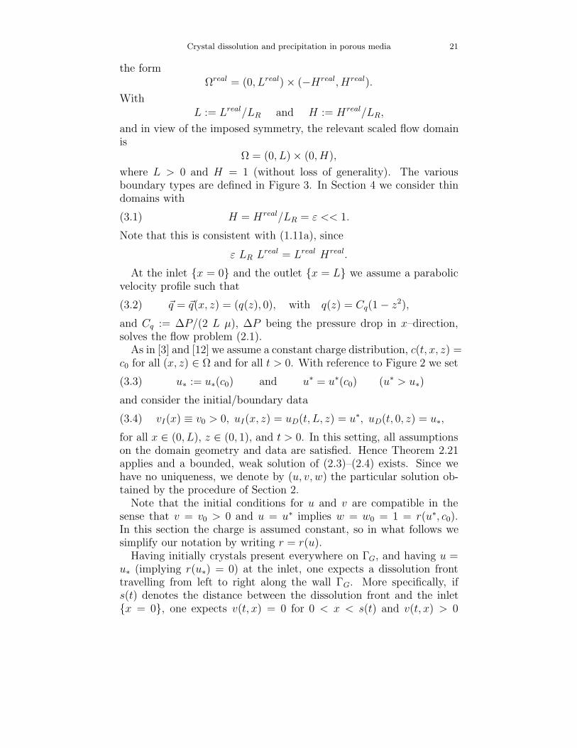
Crystal dissolution and precipitation in porous media 21
the formΩreal = (0, Lreal) × (−Hreal, Hreal).
WithL := Lreal/LR and H := Hreal/LR,
and in view of the imposed symmetry, the relevant scaled flow domainis
Ω = (0, L) × (0, H),
where L > 0 and H = 1 (without loss of generality). The variousboundary types are defined in Figure 3. In Section 4 we consider thindomains with
(3.1) H = Hreal/LR = ε << 1.
Note that this is consistent with (1.11a), since
ε LR Lreal = Lreal Hreal.
At the inlet x = 0 and the outlet x = L we assume a parabolicvelocity profile such that
(3.2) ~q = ~q(x, z) = (q(z), 0), with q(z) = Cq(1 − z2),
and Cq := ∆P/(2 L µ), ∆P being the pressure drop in x–direction,solves the flow problem (2.1).
As in [3] and [12] we assume a constant charge distribution, c(t, x, z) =c0 for all (x, z) ∈ Ω and for all t > 0. With reference to Figure 2 we set
(3.3) u∗ := u∗(c0) and u∗ = u∗(c0) (u∗ > u∗)
and consider the initial/boundary data
(3.4) vI(x) ≡ v0 > 0, uI(x, z) = uD(t, L, z) = u∗, uD(t, 0, z) = u∗,
for all x ∈ (0, L), z ∈ (0, 1), and t > 0. In this setting, all assumptionson the domain geometry and data are satisfied. Hence Theorem 2.21applies and a bounded, weak solution of (2.3)–(2.4) exists. Since wehave no uniqueness, we denote by (u, v, w) the particular solution ob-tained by the procedure of Section 2.
Note that the initial conditions for u and v are compatible in thesense that v = v0 > 0 and u = u∗ implies w = w0 = 1 = r(u∗, c0).In this section the charge is assumed constant, so in what follows wesimplify our notation by writing r = r(u).
Having initially crystals present everywhere on ΓG, and having u =u∗ (implying r(u∗) = 0) at the inlet, one expects a dissolution fronttravelling from left to right along the wall ΓG. More specifically, ifs(t) denotes the distance between the dissolution front and the inletx = 0, one expects v(t, x) = 0 for 0 < x < s(t) and v(t, x) > 0
22 C. J. van Duijn and I. S. Pop
tt*
v = 0, w = r(u)v
x=s(t)
v > 0, w = 1
v0 v(t*)x
v(t)
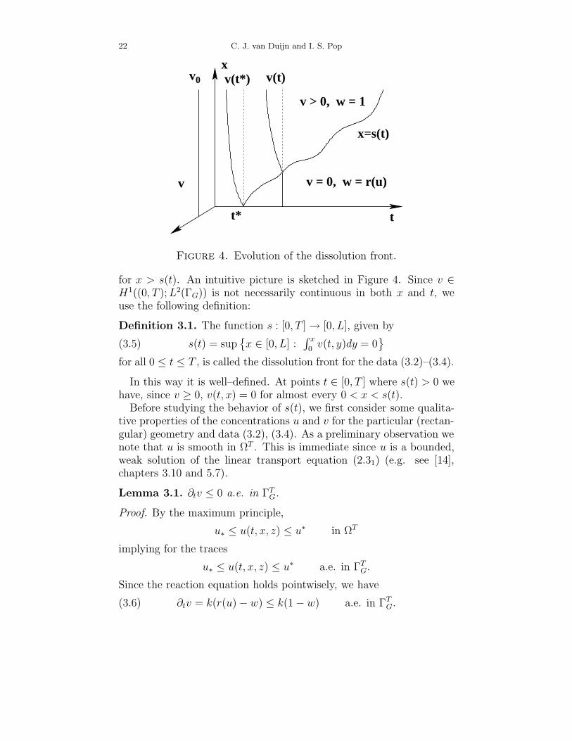
Figure 4. Evolution of the dissolution front.
for x > s(t). An intuitive picture is sketched in Figure 4. Since v ∈H1((0, T ); L2(ΓG)) is not necessarily continuous in both x and t, weuse the following definition:
Definition 3.1. The function s : [0, T ] → [0, L], given by
(3.5) s(t) = sup
x ∈ [0, L] :∫ x
0v(t, y)dy = 0
for all 0 ≤ t ≤ T , is called the dissolution front for the data (3.2)–(3.4).
In this way it is well–defined. At points t ∈ [0, T ] where s(t) > 0 wehave, since v ≥ 0, v(t, x) = 0 for almost every 0 < x < s(t).
Before studying the behavior of s(t), we first consider some qualita-tive properties of the concentrations u and v for the particular (rectan-gular) geometry and data (3.2), (3.4). As a preliminary observation wenote that u is smooth in ΩT . This is immediate since u is a bounded,weak solution of the linear transport equation (2.31) (e.g. see [14],chapters 3.10 and 5.7).
Lemma 3.1. ∂tv ≤ 0 a.e. in ΓTG.
Proof. By the maximum principle,
u∗ ≤ u(t, x, z) ≤ u∗ in ΩT
implying for the traces
u∗ ≤ u(t, x, z) ≤ u∗ a.e. in ΓTG.
Since the reaction equation holds pointwisely, we have
(3.6) ∂tv = k(r(u) − w) ≤ k(1 − w) a.e. in ΓTG.
Crystal dissolution and precipitation in porous media 23
As before, let ΓTG = S1 ∪ S2, where S1 = v = 0 and S2 = v > 0.
Then ∂tv = 0 a.e. in S1 and by (3.6), since w = 1 in S2, ∂tv ≤ 0 a.e.in S2.
Remark 3.2. Lemma 3.1 is valid for general domains, provided theboundary and initial data for u are not above u∗. In this situationprecipitation is not possible.
Lemma 3.3. ∂tu < 0 in ΩT .
Proof. To prove this result we introduce the time shift
uh(t, x, z) := u(t + h, x, z) for (t, x, z) ∈ ΩT−h,
for sufficiently small h > 0. The weak equation for u implies
(3.7)(∂t(u
h − u), ϕ)ΩT−h + D(∇(uh − u),∇ϕ)ΩT−h
−(~q(uh − u),∇ϕ)ΩT−h + εn(∂t(vh − v), ϕ)ΓT−h
G= 0.
Clearly ϕ = [uh − u]+ ∈ L2((0, T − h); H10,ΓD
(Ω)) is an admissible test
function. It satisfies ϕ|t=0 = 0 since uh ≤ u∗ at t = 0. We need toestimate the boundary term, which reads
εnk(r(uh) − r(u), [uh − u]+)ΓT−hG
− εnk(wh − w, [uh − u]+)ΓT−hG
.
The first part is non–negative by the monotonicity of r . In the secondpart we use Lemma 3.1 and the monotonicity of H, giving wh −w ≤ 0a.e. in ΓT
G. Hence the boundary term in (3.7) is non–negative. Pro-ceeding as in the proof of Lemma 2.6 gives [uh −u]+ ≡ 0 in ΩT−h. Theinterior smoothness of u now implies ∂tu ≤ 0 in ΩT . Since ∂tu is asolution of equation (2.31), it cannot have an interior maximum andstrict inequality results.
The concentrations are also monotone in the flow direction. Theargument uses the auxiliary function f : [0, T ] × [0, L] → R defined by
(3.8) f(t, x) = u∗ +(u∗ − u∗)√
Dπ
[
x
L
∫ ∞
L√t
e−ξ2
4D dξ +
∫ x√t
0
e−ξ2
4D dξ
]
.
For this and later purposes we list some properties.
24 C. J. van Duijn and I. S. Pop
Property 3.4.
(i) f ∈ L2((0, T ); H1(0, L)) ∩ C([0, T ] × [0, L]/(0, 0))
For all 0 < t < T and 0 < x < L:
(ii) ∂tf(t, x) < 0, ∂xf(t, x) > 0,
(iii) limx0
f(t, x) = u∗, limxL
f(t, x) = u∗, limt0
f(t, x) = u∗.
Proof. Since these statements follow by direct computation we omitthe proof.
Lemma 3.5.
(i) ∂xu > 0 in ΩT ;
(ii) v(t, x1) ≤ v(t, x2) for a.e. (t, x1), (t, x2) ∈ ΓTG such that x1 < x2.
Proof. We use the iteration scheme introduced in the proof of Theorem2.19 and we use Remark 2.20 about the uniqueness for Problem Pδ.In particular we use the fact that the unique solution of Pδ does notdepend on the choice of the first element u0, provided u0 ∈ KU . Goingfrom u0 to the next u1 means first solving (2.12) with u = u0 to findv0 ∈ KV as solution, and next solving (2.11) with v = v0 to findu1 ∈ KU as solution. Property 3.4 implies that f ∈ KU and that∂xf > 0 in ΩT . With u0 = f we find v0 satisfying v0(t, x + h) ≥v0(t, x) for sufficiently small h > 0 and for almost all (t, x) ∈ ΓT
h , whereΓT
h = (0, T ] × (0, L − h). We now apply the same space shift to thesolution of (2.11) in ΩT
h with Ωh = (0, L−h)× (0, 1). As in the proof ofLemma 3.3 it can be shown that u1(t, x + h, z) ≥ u1(t, x, z) in ΩT
h . Inother words, the x–monotonicity is preserved by the iterations and theunique solution (uδ, vδ) of Pδ is x–monotone. Again, this monotonicityis preserved, now along the particular subsequence δ 0 in the proofof Theorem 2.21. This proves (ii) and (i) with ∂xu ≥ 0 in ΩT . Strictinequality results again from the fact that ∂xu is a solution of (2.31).
The next lemma improves the upper bound for u.
Lemma 3.6. The weak solution U ∈ U of
(3.9)
∂tU + q(z)∂xU = D∆U, in ΩT ,−D∂zU = εnk(r(U) − 1), on ΓT
G,U = u∗, on ΓT
D ∩ x = 0,U = u∗,
on ΓTD ∩ x = L and t = 0 × Ω,
∂zU = 0, on ΓTN ,
Crystal dissolution and precipitation in porous media 25
satisfies
(i) u∗ ≤ u ≤ U ≤ u∗ in ΩT ;(ii) ∂tU < 0 and ∂xU > 0 in ΩT ;
(iii) U ∈ C(ΩT /t = 0, x = 0, 0 ≤ z ≤ 1) and U(t, x, 1) < u∗ forany 0 ≤ x < L and 0 < t ≤ T .
Proof. Following the proof of Theorem 2.19 and Remark 2.20 we obtainexistence and uniqueness of a weak solution U ∈ U . It satisfies the sameinterior smoothness as u.
(i) We test the equation for the difference U − u with ϕ = [U − u]−.Since w ≤ 1 and r is monotone, we find as before [U − u]− ≡ 0 in ΩT ,implying u ≤ U . The other inequalities follow as in Lemmas 2.6 and2.7.
(ii) As in the proofs of Lemmas 3.3 and 3.5 we apply time and spaceshifts to show the corresponding monotonicity.
(iii) Away from the corner t = 0, x = 0, 0 < z < 1, where theinitial and boundary data are incompatible, the solution is at least con-tinuous up to the boundary of ΩT . This is a consequence of chapters3.10 and 5.7 of [14]. To show the inequality we argue by contradic-tion. Suppose there exists (t0, x0) ∈ ΓT
G where U(t0, x0, 1) = u∗. thesmoothness of U up to the flat boundary ΓT
G allows us to use the strongmaximum principle, implying ∂zU(t0, x0, 1) > 0. This contradicts theboundary flux (3.92).
We are now in a position to study the qualitative behavior of thedissolution front from Definition 3.1. As a first observation, recallingr(u∗) = 1 and r(u∗) = 0, we have:
Proposition 3.7. Let
(3.10) t∗ =v0
k(r(u∗) − r(u∗))=
v0
k.
Then v > 0 a.e. in Γt∗
G and u = U in Ωt∗ .
Proof. We note that any weak solution satisfies (2.9) with u ≥ u∗ a.e.in ΓT
G. For any pair 0 ≤ x1 < x2 ≤ 1 we test (2.91) with χ(x1,x2). Thisgives
∫ x2
x1v(t, x) = v0(x2 − x1) + k
∫ t
0
∫ x2
x1r(u) − wdxdt
≥ v0(x2 − x1) + k(r(u∗) − 1)t(x2 − x1)
≥ (v0 − kt)(x2 − x1) > 0
26 C. J. van Duijn and I. S. Pop
for all 0 < t < t∗. This proves the positivity of v in Γt∗
G . With w = 1 inΓt∗
G , the concentration u satisfies (3.9) in Ωt∗ . By uniqueness we haveu = U in Ωt∗ .
The proposition implies
(3.11) s(t) = 0 for all 0 ≤ t < t∗.
Next we show that the dissolution front moves away from x = 0 fort > t∗. Therefore we call t∗ the waiting time of the dissolution front.This agrees with [4], where the same waiting time was established forthe macroscopic model.
Proposition 3.8. s(t) > 0 for all t∗ < t < T .
Proof. We first show that for each t > t∗, where s(t) < L, we have
(3.12) v(t, x) > 0 for a.e. x ∈ (s(t), L).
Let
g(x) :=
∫ x
0
v(t, y)dy for 0 ≤ x ≤ L.
Then g ∈ C([0, T ]) satisfying
g(x)
= 0, for 0 ≤ x ≤ s(t),
> 0, for s(t) < x ≤ L.
In particular, by Definition 3.1, there exists a sequence xn s(t) suchthat g(xn) > 0 and g(xn) → 0 as n → ∞. Hence there exists a relatedsequence of intervals In, with each In ⊂ (s(t), xn), such that v > 0 inIn. The x–monotonicity of v now gives v > 0 to the right of each In.This establishes (3.12).
Now suppose a t ∈ (t∗, T ] exists such that s(t) = 0. By (3.12) andLemma 3.1 we have v > 0 and w = 1 in Γt
G and u = U in Ωt. As inthe proof of Proposition 3.7 we have for each x > 0
∫ x
0v(t, y)dy = v0x + k
∫ t∗
0
∫ x
0r(U(τ, y, 1)) − 1dydτ
+k∫ t
t∗
∫ x
0r(U(τ, y, 1)) − 1dydτ
≤ k∫ t∗
0
∫ x
0r(U(τ, y, 1))dydτ
−k(t − t∗)∫ x
01 − r(U(t∗, y, 1))dy.
Crystal dissolution and precipitation in porous media 27
0 x = s(t) x
t
(a)
t
x + L
x = s(t)
v = 0
v > 0v > 0t*
ζ x = s(t)0 x
t
t
L
x = s(t)
v = 0
v > 0v > 0t* R
(b)x − ζ
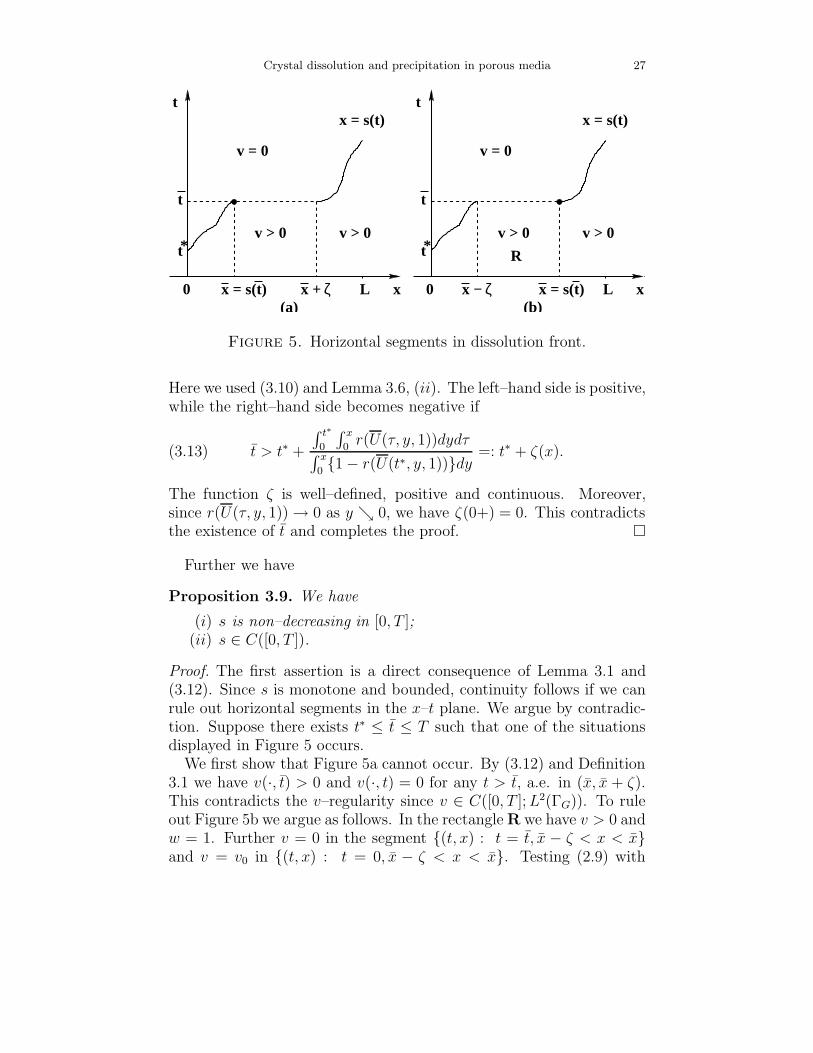
Figure 5. Horizontal segments in dissolution front.
Here we used (3.10) and Lemma 3.6, (ii). The left–hand side is positive,while the right–hand side becomes negative if
(3.13) t > t∗ +
∫ t∗
0
∫ x
0r(U(τ, y, 1))dydτ
∫ x
01 − r(U(t∗, y, 1))dy
=: t∗ + ζ(x).
The function ζ is well–defined, positive and continuous. Moreover,since r(U(τ, y, 1)) → 0 as y 0, we have ζ(0+) = 0. This contradictsthe existence of t and completes the proof.
Further we have
Proposition 3.9. We have
(i) s is non–decreasing in [0, T ];(ii) s ∈ C([0, T ]).
Proof. The first assertion is a direct consequence of Lemma 3.1 and(3.12). Since s is monotone and bounded, continuity follows if we canrule out horizontal segments in the x–t plane. We argue by contradic-tion. Suppose there exists t∗ ≤ t ≤ T such that one of the situationsdisplayed in Figure 5 occurs.
We first show that Figure 5a cannot occur. By (3.12) and Definition3.1 we have v(·, t) > 0 and v(·, t) = 0 for any t > t, a.e. in (x, x + ζ).This contradicts the v–regularity since v ∈ C([0, T ]; L2(ΓG)). To ruleout Figure 5b we argue as follows. In the rectangle R we have v > 0 andw = 1. Further v = 0 in the segment (t, x) : t = t, x − ζ < x < xand v = v0 in (t, x) : t = 0, x − ζ < x < x. Testing (2.9) with
28 C. J. van Duijn and I. S. Pop
θ = χ(0,t)ϕ(x), ϕ ∈ L2((x − ζ, x)), gives
∫ x
x−ζ
(v(t, x) − v0)ϕ(x)dx = k
∫
R
(r(u(τ, x, 1))− 1)ϕ(x)dxdτ,
or∫ x
x−ζ
∫ t
0
[1 − r(u(τ, x, 1))]dτ − v0
k
ϕ(x)dx = 0.
Since this holds for any ϕ we have, in fact,
(3.14)
∫ t
0
[1 − r(u(τ, x, 1))]dτ =v0
ka.e. in (x − ζ, x).
Since u is strictly increasing with respect to x in the interior of ΩT ,its trace is non–decreasing in ΓT
G and in particular in any segmentt = τ, x − ζ < x < x in R. Combined with equality (3.14) thisimplies u(τ, ·, 1) is constant in (x − ζ, x) for each 0 < τ < t. But inΩt∗ we have u = U . Hence U(τ, ·, 1) is also constant in (x − ζ, x) foreach 0 < τ < t∗. This gives a contradiction because U(t) is strictlyincreasing in ΓG for any t > 0. To see this we consider the differenceUh(t, x, z) := U(t, x + h, z) − U(t, x, z). It satisfies (3.91) in ΩT
h and,by Lemma 3.6, it is continuous up to the boundary for all t > 0.Further Uh > 0 in ΩT
h and, for h < ζ, Uh = 0 in the boundary setΓt∗
G ∩ x − ζ < x < x − h. By the strong maximum principle thismeans ∂zUh < 0 in that set, while the boundary condition implies∂zUh = 0.
We now improve the monotonicity of the front by showing that fort > t∗ no additional waiting times occur in 0 < x < L. In otherwords:
Proposition 3.10. s is strictly increasing when 0 < s < L.
Proof. By Proposition 3.9 it suffices to rule out vertical segments inthe x–t plane. We argue again by contradiction. Suppose, as in Figure6, that there exists s0 ∈ (0, L) and t1 < t2 such that s(t) = s0 fort1 ≤ t ≤ t2. Here we take t1 minimal in the sense that s(t) < s0 forall t < t1. We first estimate v in x > s0. By (3.12) and Lemma3.1, we have v > 0 and w = 1 a.e. in (t, x) : t < t2, x > s0.Hence, with µ > 0 and fixed, we have for any t ≤ t1 and for almost all
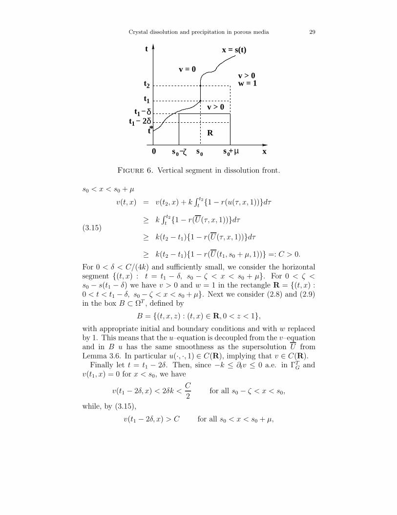
Crystal dissolution and precipitation in porous media 29
t*
t2
t1
1t −
1t − 2
0s 0 µs +
t
v = 0
0 x
x = s(t)
v > 0
v > 0w = 1
Rδδ
0s − ζ
Figure 6. Vertical segment in dissolution front.
s0 < x < s0 + µ
(3.15)
v(t, x) = v(t2, x) + k∫ t2
t1 − r(u(τ, x, 1))dτ
≥ k∫ t2
t1 − r(U(τ, x, 1))dτ
≥ k(t2 − t1)1 − r(U(τ, x, 1))dτ
≥ k(t2 − t1)1 − r(U(t1, s0 + µ, 1)) =: C > 0.
For 0 < δ < C/(4k) and sufficiently small, we consider the horizontalsegment (t, x) : t = t1 − δ, s0 − ζ < x < s0 + µ. For 0 < ζ <s0 − s(t1 − δ) we have v > 0 and w = 1 in the rectangle R = (t, x) :0 < t < t1 − δ, s0 − ζ < x < s0 + µ. Next we consider (2.8) and (2.9)in the box B ⊂ ΩT , defined by
B = (t, x, z) : (t, x) ∈ R, 0 < z < 1,with appropriate initial and boundary conditions and with w replacedby 1. This means that the u–equation is decoupled from the v–equationand in B u has the same smoothness as the supersolution U fromLemma 3.6. In particular u(·, ·, 1) ∈ C(R), implying that v ∈ C(R).
Finally let t = t1 − 2δ. Then, since −k ≤ ∂tv ≤ 0 a.e. in ΓTG and
v(t1, x) = 0 for x < s0, we have
v(t1 − 2δ, x) < 2δk <C
2for all s0 − ζ < x < s0,
while, by (3.15),
v(t1 − 2δ, x) > C for all s0 < x < s0 + µ,
30 C. J. van Duijn and I. S. Pop
contradicting the continuity of v in R.
We conclude the qualitative statements about s with the estimate:
Proposition 3.11. There exists a constant C > 0, not depending onL and T , such that
s(t) ≤ Ct2 for all t > 0.
Proof. Since v = 0 in (t, x) : t∗ < t < T, 0 < x < s(t), −k ≤ ∂tv ≤ 0a.e. in ΓT
G and s is strictly increasing, we deduce that v(t, s(t)) = 0for almost all t ∈ (t∗, T ) where s(t) < L. We use this observation andw = 1 a.e. in (t, x) : 0 < t < T, s(t) < x < L to derive from (2.41)the free boundary equation
(3.16)v0
k=
∫ t
0
1 − r(u(τ, s(t), 1))dτ
for those t ∈ (t∗, T ) where s(t) < L. With Lr given in Remark 2.9 wehave
1 − r(u) = r(u∗) − r(u) ≤ Lr(u∗ − u).
We estimate
(3.17) u∗ − u ≤ (u∗ − u∗)ξ in ΩT ,
where ξ is the one–dimensional solution satisfying
(3.18)
∂tξ + Cq∂xξ = D∂2x2ξ in (t, x) : t > 0, x > 0,
ξ(0, t) = 1 for t > 0, ,
ξ(x, 0) = 0 for x > 0.
Combining (3.16) and (3.17) gives
(3.19) K :=v0
kLr(u∗ − u∗)≤
∫ t
0
ξ(τ, s(t))dτ ≤ tξ(t, s(t)),
where we used ∂tξ > 0. We note here that K < t∗. Since ∂xξ < 0 wealso have
s(t)ξ(t, s(t)) ≤∫ s(t)
0ξ(t, y)dy =
∫ s(t)
0
(
∫ t
0∂tξ(τ, y)dτ
)
dy
=∫ t
0
(
∫ s(t)
0∂tξ(τ, y)dy
)
dτ
≤∫ t
0(−D∂xξ(τ, 0) − Cqξ(τ, s(t)))dτ + Cqt,
or
(3.20) s(t)ξ(t, s(t)) + Cq
∫ t
0
ξ(τ, s(t))dτ ≤ −D
∫ t
0
∂xξ(τ, 0) + Cqt.
Crystal dissolution and precipitation in porous media 31
We estimate the flux term on the right by the solution of (3.18) withCq = 0. This is a subsolution for the complete (3.18). It is closelyrelated to (3.8) with L = ∞. Using this subsolution and (3.19) in(3.20) gives
s(t)ξ(t, s(t)) ≤ 2
√
D
πt1/2 + Cq(t − K).
Again using (3.19) yields
s(t) <Cq
Kt(t − K) +
2
K
√
D
πt3/2 for t > t∗.
Remark 3.12. So far we discussed the dissolution front for the specialinitial/boundary data (3.4). Similar results can be obtained for moregeneral data. For instance, if
(3.21)
vI(x) ≥ 0 (6≡ 0), uI(x, z) ≤ u∗,
u∗ ≤ uD(t, 0, z) < uD(t, L, z) ≤ u∗,
for all x ∈ (0, L), z ∈ (0, 1) and t > 0, and if c = c0 in ΩT , precipitationis not possible. This follows from the maximum principle for u, givingu ≤ u∗ and thus ∂tv ≤ 0 in ΓT
G. Hence, for data satisfying (3.21), onlydissolution occurs and this will strongly depend on the specific form ofthe functions in (3.21). As an example, let vI be hat-shaped with Inparticular, assuming that vI is “hat–shaped” with
vI(x) =
v0 > 0, if x ∈ [x1, x2] ⊂ (0, L),0, otherwise ,
and let u satisfy (3.4). Then we find two dissolution fronts: a left frontstarting at x = x1 with waiting time t∗1, and a right front starting atx = x2 with waiting time t∗2. The waiting times are determined by thefree boundary equation (3.16) at x1 and x2, i. e.
v0
k=
∫ t
0
1 − r(u(τ, xi, 1))dτ for i = 1, 2.
Here ions enter the fluid only when x1 < x < x2. Therefore the x–monotonicity of u does not hold anymore and it is not clear which ofthe two waiting times is the biggest. After t∗1, the left front moves tothe right and after t∗2, the right front moves to the left. They will meetat a finite t∗ when all crystals are dissolved.
32 C. J. van Duijn and I. S. Pop
Remark 3.13. Precipitation or precipitation fronts occur if uI and/oruD are above u∗. This is the only possibility for ∂tv > 0 somewhere inΓT
G. For instance, if
vI(x) = 0, uI(x, z) = uD(t, L, z) = u ≤ u∗, uD(t, 0, z) = u > u∗,
for all x ∈ (0, L), z ∈ (0, 1) and t > 0, and if c = c0 in ΩT , wefind a precipitation front moving from left to right on ΓG. If u = u∗
then, by the maximum principle for u, u > u∗ in ΩT and instantaneousprecipitation occurs everywhere in ΓG. The condition u > u∗ meansthat the injected fluid is oversaturated.
4. Thin strips
In this section we maintain the framework of Section 3, but assumeadditionally that the strip is thin with H given by (3.1). Using thesame value for the scaling factor in (1.11b), and thus assuming thatfor all ε > 0 the system contains about the same number of moles forboth crystals and solutes, we study the limit as ε 0. As a result werecover the one–dimensional reactive solute transport model proposedin [12] and [3].
To stress the dependence on ε we use superscripts as, for instance,in
(4.1) Ωε = (0, L) × (0, ε).
To ensure that the average flow in x–direction does not vanish andremains constant as ε 0 we impose
(4.2) ~qε(x, z) = (qε(z), 0), with qε(z) =3
2Q
(
1 − z2/ε2)
,
where Q = 1ε
∫ ε
0qε(z)dz is a prescribed average flow.
Remark 4.1. The thin strip is a simplified model for the void spacebetween two grains in a porous medium. If the pressure gradient is oforder 1, a velocity profile as in (4.2) can only be achieved if the scaledfluid viscosity µ = O(ε2). This assumption is commonly encounteredwhen homogenizing periodic structures – see for instance [9] and [16].It prevents one from obtaining a trivial upscaled velocity correspondingto an immobile fluid as ε 0.
Imposing the same initial and boundary conditions as in Section 3,we obtain a bounded weak solution (uε, vε, wε) and a correspondingdissolution front sε satisfying all properties discussed in that section.
The scaling ξ = z/ε, with 0 < ξ < 1, transforms the domain Ωε backto Ω = (0, L) × (0, 1). Further qε(z) = q(ξ) := 3
2Q(1 − ξ2). In terms of
Crystal dissolution and precipitation in porous media 33
x, ξ and t the solution (uε, vε, wε) satisfies
(4.3)(∂tu
ε, ϕ)ΩT + D(∂xuε, ∂xϕ)ΩT + D
ε2 (∂ξuε, ∂ξϕ)ΩT
+(q∂xuε, ϕ)ΩT + n(∂tv
ε, ϕ)ΓTG
= 0,
(4.4)(∂tv
ε, θ)ΓTG
= k(r(uε) − wε, θ)ΓTG
wε ∈ H(vε), a.e. in ΓTG,
for all (ϕ, θ) ∈ L2((0, T ); H10,ΓD
(Ω)) × L2(ΓTG).
Next we define the average
(4.5) U ε(t, x) :=
∫ 1
0
uε(t, x, ξ) dξ.
The properties of uε imply that Uε ∈ Uav := L2((0, T ); H1(0, L)) ∩H1((0, T ); H−1(0, L)) and satisfies Uε(t, 0) = u∗, and U ε(t, L) = Uε(0, x)= u∗. Let Ωav := (0, L). Writing for consistency of notation V ε(t, x) :=vε(t, x) and W ε(t, x) := wε(t, x), and testing (4.3) with ξ–independentfunctions, gives
(4.6)
(∂tUε, ϕ)ΩT
av+ D(∂xU
ε, ∂xϕ)ΩTav
+ (∂xUε, ϕ)ΩT
av
+n(∂tVε, ϕ)ΩT
av=
(
∫ 1
0(Q − q)∂xu
ε, ϕ)
ΩTav
,
for all ϕ ∈ L2((0, T ); H10(Ωav)). Further,
(4.7)
(∂tVε, θ)ΩT
av= k(r(U ε) − W ε, θ)ΩT
av
+ k(r(uε(·, ·, 1)) − r(U ε), θ)ΩTav
W ε ∈ H(V ε), a.e. in ΩTav,
for all θ ∈ L2(ΩTav).
Below we make precise that as ε 0, the triple (Uε, V ε, W ε) con-verges towards (U, V, W ), being the weak solution of the reactive solutetransport equations
∂t(U + nV ) + Q∂xU = D∂2xxU,
∂tV = k(r(U) − W ),
W ∈ H(V ),
in ΩTav. These equations were proposed in [12] and [3] to describe crystal
dissolution in a homogenized porous medium. The appropriate weakformulation is:
34 C. J. van Duijn and I. S. Pop
Problem Pav: Find (U, V, W ) ∈ Uav ×V ×W such that U(t, 0) = u∗,U(t, L) = U(0, x) = u∗, V (0, x) = v0, and
(4.8)(∂tU, ϕ)ΩT
av+ D(∂xU, ∂xϕ)ΩT
av
+(Q∂xU, ϕ)ΩTav
+ n(∂tV, ϕ)ΩTav
= 0,
(4.9)(∂tV, θ)ΩT
av= k(r(U) − W, θ)ΩT
av,
W ∈ H(V ), a.e. in ΩTav,
for all (ϕ, θ) ∈ L2((0, T ); H10(Ωav)) × L2(ΩT
av).
We start with some a–priori estimates.
Lemma 4.2. For any T > 0, there exists a constant C > 0 such that
‖uε(t)‖2Ω + D‖∂xu
ε‖2Ωt +
D
ε2‖∂ξu
ε‖2Ωt ≤ C,
for all ε > 0 and for all 0 ≤ t ≤ T .
Proof. The proof is immediate after testing (4.3) with ϕ = χ(0,t)(uε −
u∗ − (u∗ − u∗)x/L).
The following proposition uses the idea of the trace theorem; see forinstance [5], chapter 5.5.
Proposition 4.3. Let f ∈ H1(Ω) and let F : [0, L] → R be defined by
F (x) =∫ 1
0f(x, ξ) dξ. Then, in the sense of traces,
‖f(·, ξ0) − F‖(0,L) ≤ ‖∂ξf‖Ω
for each ξ0 ∈ [0, 1].
Proof. We demonstrate the inequality for f ∈ C1(Ω). The extensionto f ∈ H1(Ω) in the sense of traces follows from the usual densityargument. For arbitrary ξ0 ∈ [0, L] we have
‖f(·, 1) − F‖2(0,L) =
∫ L
0
f(x, ξ0) −∫ 1
0f(x, ζ) dζ
2
dx
=∫ L
0
∫ 1
0(f(x, ξ0) − f(x, ζ))dζ
2
dx
=∫ L
0
∫ 1
0
(
∫ ξ0ζ
∂ξf(x, ξ) dξ)
dζ2
dx ≤ ‖∂ξf‖2Ω
Combining Lemma 4.2 and Proposition 4.3 gives
Crystal dissolution and precipitation in porous media 35
Lemma 4.4. For any T > 0 we have
‖uε(·, ·, ξ0) − Uε‖2ΩT
av≤ ε2
DC.
for all ε > 0 and for all ξ0 ∈ [0, 1]. Here C is the constant from Lemma4.2.
Proof. For almost every t ∈ (0, T ) we apply Proposition 4.3 to uε(t, ·, ·).The assertion now follows from the gradient estimate in Lemma 4.2.
The weak formulations for Uε (4.6) and U (4.8) differ by the term
(4.10a) T ε1 (ϕ) :=
(∫ 1
0
(Q − q)∂xuε, ϕ
)
ΩTav
,
the ones for (V ε, W ε) (4.7) and (V, W ) (4.9) by
(4.10b) T ε2 (θ) := k(r(uε(·, ·, 1)) − r(U ε), θ)ΩT
av.
These terms are estimated in the lemma below.
Lemma 4.5. For any T > 0 we have
|T ε1 (ϕ)| ≤ εQ
√
C5D
‖∂xϕ‖L2(ΩTav),
|T ε2 (θ)| ≤ εkLr
√
CD
‖θ‖L2(ΩTav),
for all ϕ ∈ L2((0, T ); H10(Ωav)), θ ∈ L2(ΩT
av) and for all ε > 0. HereC is the constant from Lemma 4.2 and Lr the Lipschitz constant fromRemark 2.9.
Proof. We integrate T1 by parts and subtract 0 = (∫ 1
0(Q−q)Uε, ∂xϕ)ΩT
av.
Then Cauchy’s inequality and Lemma 4.4 provide the first estimate.The Lipschitz continuity of r and again Lemma 4.4 give the secondone.
We are now in a position to estimate the average Uε and V ε, W ε.
Lemma 4.6. For any T > 0 we have
i) u∗ ≤ Uε ≤ u∗, 0 ≤ V ε ≤ v0, 0 ≤ W ε ≤ 1 a.e.in ΩTav;
ii) there exists a constant C > 0 such that
‖U ε(t)‖2Ωav
+ D‖∂xUε‖2
Ωtav
≤ C,
‖∂tUε‖2
L2((0,t);H−1(Ωav)) ≤ C(
1 + ε2
D
)
.
‖V ε(t)‖2Ωav
+ ‖∂tVε‖2
Ωtav
≤ C.
for all 0 < t ≤ T and for all ε > 0.
36 C. J. van Duijn and I. S. Pop
Proof. The L∞ bounds are straightforward. They directly imply theL2–bounds for U ε(t) and V ε(t). The estimate on ∂xU
ε follows fromLemma 4.2 and the estimate on ∂tV
ε is obtained by testing (4.7) withθ = χ(0,t)∂tV
ε. Finally, (4.6) yields
|(∂tUε, ϕ)Ωt
av| ≤ D‖∂xU
ε‖Ωtav‖∂xϕ‖Ωt
av+ Q‖U ε‖Ωt
av‖∂xϕ‖Ωt
av
+n‖∂tVε‖Ωt
av‖ϕ‖Ωt
av+ |T ε
1 (ϕ)|
for all ϕ ∈ L2((0, t); H10(Ωav)). Then the previous estimates and Lemma
4.5 give the H−1 bound.
The estimates in Lemma 4.6 imply that
U εε>0 is uniformly bounded in L∞(ΩTav) ∩ L2((0, T ); H1(Ωav))
∩H1((0, T ); H−1(Ωav));
V εε>0 is uniformly bounded in L∞(ΩTav) ∩ H1((0, T ); L2(Ωav));
W εε>0 is uniformly bounded in L∞(ΩTav).
Compactness arguments give the existence of a triple (U, V, W ) ∈ Uav×H1((0, T ); L2(Ωav)) × L∞(ΩT
av) and a sequence ε 0 such that
a) U ε → U weakly in L2((0, T ); H1(Ωav)),
b) ∂tUε → ∂tU weakly in L2((0, T ); H−1(Ωav)),
c) V ε → V weakly in L2(ΩTav),
d) ∂tVε → ∂tV weakly in L2(ΩT
av),e) W ε → W weakly–star in L∞(ΩT
av).
The following theorem shows that the limit (U, V, W ) thus obtained isthe unique solution of Problem Pav.
Theorem 4.7. Problem Pav has the triple (U, V, W ) as its unique weaksolution.
Proof. We first demonstrate uniqueness. It implies that (Uε, V ε, W ε)ε>0
converges towards (U, V, W ) along any sequence ε 0. Let (U1, V1, W1)and (U2, V2, W2) both solve Problem Pav. One easily verifies thatu∗ ≤ U1, U2 ≤ u∗ a.e. in ΩT
av. Set
U := U1 − U2, and V := V1 − V2 in ΩTav.
To simplify notation we write below (·, ·) and ‖·‖ instead of (·, ·)Ωav and‖ · ‖Ωav , respectively. In the spirit of [1], we test (4.9) with θ(t, x) =χ(0,t)V for any 0 < t ≤ T . Using the monotonicity of H and the
Crystal dissolution and precipitation in porous media 37
Lipschitz continuity of r, we obtain
‖V (t)‖2 ≤ k2L2r
∫ t
0
‖U(τ)‖2dτ +
∫ t
0
‖V (τ)‖2dτ,
for all t ≤ T . Applying Gronwall’s lemma gives
(4.11)‖V (t)‖2 ≤ etk2L2
r
∫ t
0‖U(τ)‖2dτ,
∫ t
0‖V (τ)‖2dτ ≤ (et − 1) k2L2
r
∫ t
0‖U(τ)‖2dτ.
The difference U satisfies
(4.12) (∂tU, ϕ) + D(∂xU, ∂xϕ) + Q(∂xU, ϕ) + n(∂tV, ϕ) = 0
for all ϕ ∈ L2((0, T ); H10(Ωav)). For fixed s ≤ T , chosen arbitrarily, we
test (4.12) with ϕ(t, x) = χ(0,s)
∫ s
tU(τ, x)dτ and evaluate each of the
resulting terms. In a straightforward way we obtain∫ s
0
‖U(t)‖2dt+D‖∂xϕ(0)‖2 ≤ 2n2
∫ s
0
‖V (t)‖2dt+2Q2
∫ s
0
‖∂xϕ(t)‖2dt.
Using (4.11) and taking s ≤ ln (1 + 1/(2nkLr)2) gives
(4.13)1
2
∫ s
0
‖U(t)‖2dt + D‖∂xϕ(0)‖2 ≤ 2Q2
∫ s
0
‖∂xϕ(t)‖2dt.
Estimating∫ s
0‖∂xϕ(t)‖2dt =
∫ s
0
∫ L
0
∣
∣
∫ s
t∂xU(τ, x)dτ
∣
∣
2dxdt
≤ 2∫ s
0
∫ L
0
∣
∣
∫ s
0∂xU(τ, x)dτ
∣
∣
2dxdt + 2
∫ s
0
∫ L
0
∣
∣
∣
∫ t
0∂xU(τ, x)dτ
∣
∣
∣
2
dxdt
= 2s∫ L
0
∣
∣
∫ s
0∂xU(τ, x)dτ
∣
∣
2dx + 2
∫ s
0
∫ L
0
∣
∣
∣
∫ t
0∂xU(τ, x)dτ
∣
∣
∣
2
dxdt
in (4.13) and taking further s ≤ D8Q2 we obtain
(4.14)
∫ s
0
‖U(t)‖2dt + Dζ(s) ≤ 8Q2
∫ s
0
ζ(t) dt,
where ζ(t) =∫ L
0
∣
∣
∣
∫ t
0∂xU(τ, x) dτ
∣
∣
∣
2
dx. By Gronwall’s lemma we deduce
ζ(s) = 0,
and consequently∫ s
0
‖U(t)‖2dt = 0,
for all 0 ≤ s ≤ min
D8Q2 , ln
(
1 + 1(2nkLr)2
)
. This establishes unique-ness.
38 C. J. van Duijn and I. S. Pop
To obtain existence we consider (4.6)–(4.71). By Lemma 4.5 andthe convergence properties of Uε, V ε and W ε we directly obtain that(U, V, W ) satisfies (4.8)–(4.91). To establish (4.72) we argue as in theproof of Theorem 2.21. The essential difference is that here, from (4.71),
∂tVε = k(r(U ε) − W ε) + k(r(uε(·, ·, 1))− r(U ε))
and thus
(4.15) V ε = v0 + k
∫ t
0
(r(U ε) − W ε) + k
∫ t
0
(r(uε(·, ·, 1)) − r(U ε))
a.e. in ΩTav. By Lemma 4.4, however, the last term on the right in
(4.15) vanishes as ε 0. Therefore we can proceed exactly along thelines of the proof of Theorem 2.21. We omit the details.
Remark 4.8. Theorem 4.7 gives existence and uniqueness for the onedimensional case of the model proposed in [12] and [3]. In the multi–dimensional case existence can be obtained by regularization argumentsas used in Section 2. The uniqueness proof cannot be extended straight-forwardly to the multi–dimensional case, since v is defined on a lowerdimensional manifold. In the estimates we then have to use trace re-sults, involving also gradients of U , in inequalities like (4.11).
Remark 4.9. As in Theorem 2.21, in addition to W ∈ H(V ) we havethat W = r(U) a.e. in V = 0 ∩ ΩT
av.
As noted before there exists for each ε > 0 a dissolution front Sε thatseparates the region where all crystals are dissolved from the regionwhere crystals are still present. In particular,
Sε(t) =
0, for 0 ≤ t ≤ t∗ =v0
k,
continuous and strictly increasing for t > t∗
and
V ε(t, x) =
0, if 0 < x < Sε(t) and t > t∗,
> 0, if x > Sε(t) and t > 0
for all ε > 0. These properties carry over in the averaging process.Related to Problem Pav we call S : [0, T ] → [0, L], defined by
S(t) := sup
0 ≤ x ≤ L :
∫ x
0
V (t, y)dy = 0
for 0 ≤ t ≤ T , the dissolution front.Then we have
Crystal dissolution and precipitation in porous media 39
Theorem 4.10.
(i) S(t) =
0, 0 ≤ t ≤ t∗,
> 0, t∗ < t ≤ T ;
(ii) S ∈ C([0, T ]) and strictly increasing when 0 < S < L;
(iii) V (t, x) = 0, W (t, x) = r(U(t, x)) for t > t∗ and 0 < x < S(t);
(iv) V (t, x) > 0, W (t, x) = 1 for t > 0 and S(t) < x ≤ L;
(v) along any sequence ε 0, Sε → S pointwisely in [0, T ].
Proof. Assertions (i)–(iv) are proven by the methods and ideas devel-oped in Section 3. We omit the details. To show (v) we first note thatSε(t) = S(t) = 0 for any ε > 0 and for all 0 ≤ t ≤ t∗. Thus it remainsto consider t > t∗.
With t ∈ (t∗, T ] chosen arbitrarily we show that limε0 Sε(t) = S(t)along any sequence ε 0. To this aim we first observe that V (t, x) = 0for almost every x ∈ [0, L] where lim infε0 V ε(t, x) = 0. This followsfrom an argument similar to the one used in the proof of Theorem 2.21.Hence V (t, x) > 0 implies lim infε0 V ε(t, x) > 0, so
(4.16) S(t) ≥ Sε(t)
if ε is small enough.Next assume that there exists a µ > 0 and a sequence ε 0 such
that
Sε(t) ≤ S(t) − µ.
Then by the monotonicity of Sε and the continuity of S, there existst0 < t such that
Sε(τ) ≤ S(t) − µ < S(t) − µ
2< S(τ)
for all t0 ≤ τ ≤ t. Consequently, along this sequence ε 0,
V ε > 0 and W ε = 1 a.e. in R,
while
V = 0 and W = r(U) a.e. in R,
where R denotes the rectangle (t0, t) × (S(t) − µ, S(t) − µ2).
Applying Lemma 3.6 to uε, since Uε converges almost everywhere toU we directly obtain
U ≤∫ 1
0
U(·, ·, ξ) dξ < u∗ a.e. in ΩTav
40 C. J. van Duijn and I. S. Pop
and thusr(U) < 1 a.e. in R.
This contradicts the weak–star convergence of W ε towards W and,together with (4.16) completes the proof of assertion (v).
Remark 4.11. In the previous analysis we assumed D = O(1). Differentregimes would occur when considering D = O(εγ). Taking γ ∈ (0, 2),formal upscaling would lead to a hyperbolic version of (4.8), in whichthe diffusive term has vanished. We expect the case γ ≥ 2 to be moreinvolved, and the corresponding upscaled equations more difficult toobtain.
5. Numerical example
In this section we present some numerical results obtained for theparticular geometry considered in Sections 3 and 4. Specifically, for L =20.0 and a given ε > 0 we consider the thin strip Ωε = (0, L) × (0, ε),which is transformed back to Ω = (0, L)×(0, 1) by the scaling proposedin Section 4. This leads to the model given in (4.3)–(4.4).
We have used the following parameters and rate function:
D = Q = m = n = 1.0, k = 0.9, and r(u, c) =10
9[u]+[u − c]+.
The total charge is kept constant, with c = 0.1. The fluid velocity qis given in (4.2). The initial and (external) boundary conditions arespecified in (3.4), with
u∗ = 0.1, u∗ = 1.0, and v0 = 1.0.
Computations are performed for two values of ε: ε = 1 and ε = 0.2.We computed up to T = 30. The choice L = 20 ensures that, withinthe specified time, the influence of the boundary condition at the outletis minimal. Discretization in space is obtained by finite differences ona regular grid of size h = 0.05. For the transport term we have applieda standard first order upwinding. For the time discretization we haveused the forward Euler scheme with a fixed time step τ = 10−5. By thischoice the CFL–condition is satisfied. As mentioned in the appendixof [3] (see also Theorem 2.21), we set w = r(u) whenever v = 0.
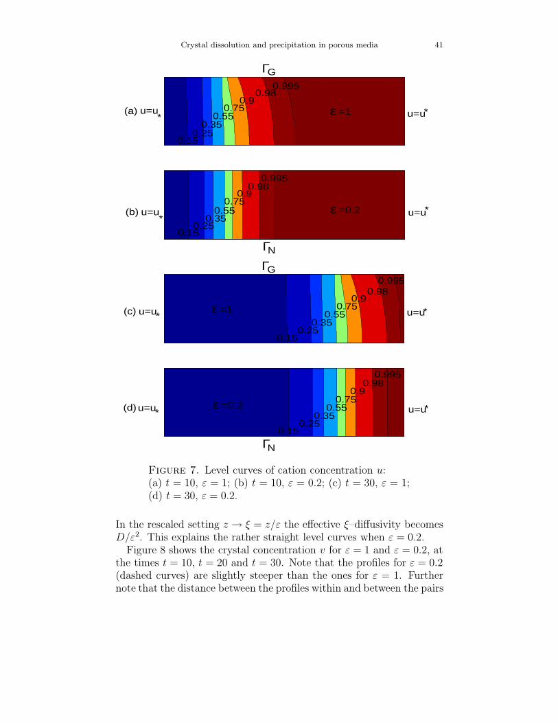
Figure 7 displays level curves of the cation concentration u. In thefisrt pair t = 10, with ε = 1 in Figure 7a and ε = 0.2 in Figure 7b. Inthe second pair t = 30, with ε = 1 in Figure 7c and ε = 0.2 in Figure7d. The level curves are curved due to the parabolic velocity profilewhich attains its largest value at the centre of the strip, here denotedby ΓN . Along the wall ΓG, cations are being fed to the fluid by thechemical reactions. This causes an increase in longitudinal spreading.
Crystal dissolution and precipitation in porous media 41
0.150.25
0.350.55
0.750.9
0.980.995
0.150.25
0.350.55
0.750.9
0.980.995
u=u *
* u=u * u=u
* u=u
Γ G
N Γ
ε =1
ε =0.2
(a)
(b)
0.150.25
0.350.55
0.750.9
0.980.995
0.150.25
0.350.55
0.750.9
0.980.995
u=u *
* u=u * u=u
* u=u
Γ G
N Γ
ε =1
ε =0.2
(c)
(d)
Figure 7. Level curves of cation concentration u:(a) t = 10, ε = 1; (b) t = 10, ε = 0.2; (c) t = 30, ε = 1;(d) t = 30, ε = 0.2.
In the rescaled setting z → ξ = z/ε the effective ξ–diffusivity becomesD/ε2. This explains the rather straight level curves when ε = 0.2.
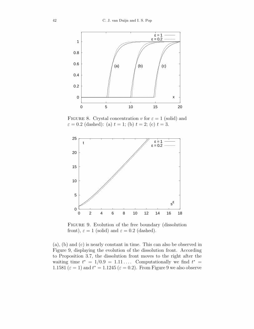
Figure 8 shows the crystal concentration v for ε = 1 and ε = 0.2, atthe times t = 10, t = 20 and t = 30. Note that the profiles for ε = 0.2(dashed curves) are slightly steeper than the ones for ε = 1. Furthernote that the distance between the profiles within and between the pairs
42 C. J. van Duijn and I. S. Pop
0
0.2
0.4
0.6
0.8
1
0 5 10 15 20
x
(a) (b) (c)
ε = 1ε = 0.2
Figure 8. Crystal concentration v for ε = 1 (solid) andε = 0.2 (dashed): (a) t = 1; (b) t = 2; (c) t = 3.
0
5
10
15
20
25
0 2 4 6 8 10 12 14 16 18
t
sε
ε = 1 ε = 0.2
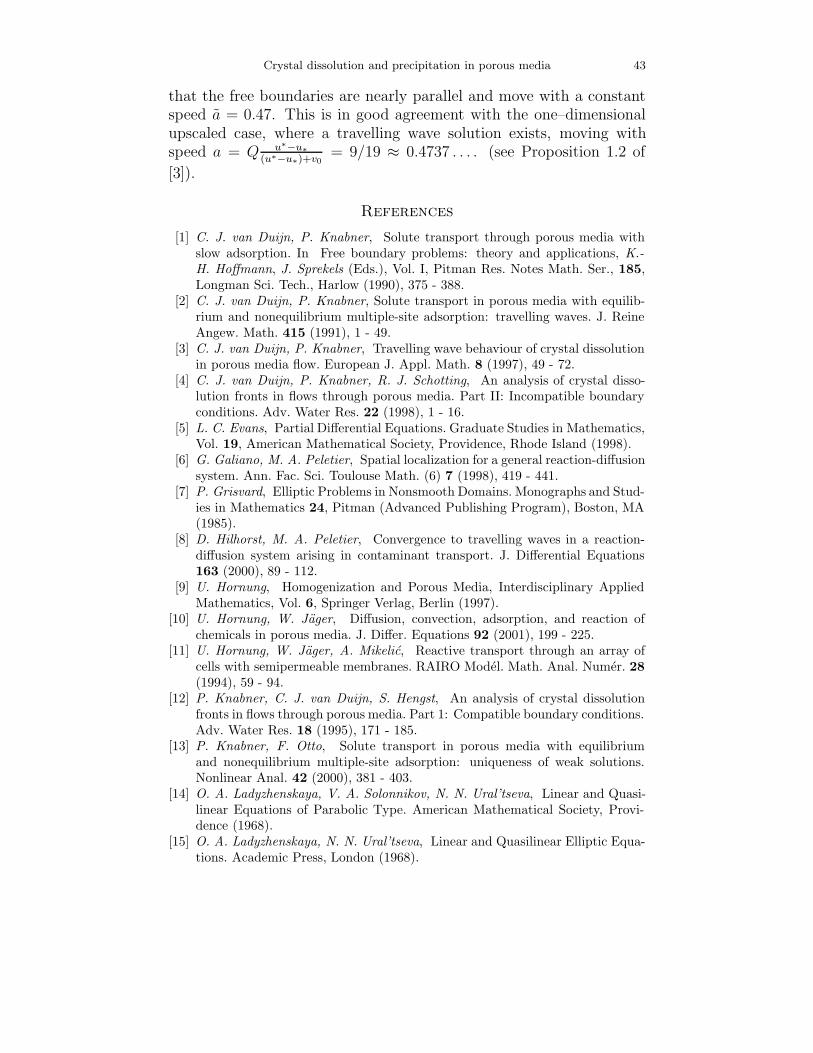
Figure 9. Evolution of the free boundary (dissolutionfront), ε = 1 (solid) and ε = 0.2 (dashed).
(a), (b) and (c) is nearly constant in time. This can also be observed inFigure 9, displaying the evolution of the dissolution front. Accordingto Proposition 3.7, the dissolution front moves to the right after thewaiting time t∗ = 1/0.9 = 1.11 . . . . Computationally we find t∗ =1.1581 (ε = 1) and t∗ = 1.1245 (ε = 0.2). From Figure 9 we also observe
Crystal dissolution and precipitation in porous media 43
that the free boundaries are nearly parallel and move with a constantspeed a = 0.47. This is in good agreement with the one–dimensionalupscaled case, where a travelling wave solution exists, moving withspeed a = Q u∗−u∗
(u∗−u∗)+v0= 9/19 ≈ 0.4737 . . . . (see Proposition 1.2 of
[3]).
References
[1] C. J. van Duijn, P. Knabner, Solute transport through porous media withslow adsorption. In Free boundary problems: theory and applications, K.-
H. Hoffmann, J. Sprekels (Eds.), Vol. I, Pitman Res. Notes Math. Ser., 185,Longman Sci. Tech., Harlow (1990), 375 - 388.
[2] C. J. van Duijn, P. Knabner, Solute transport in porous media with equilib-rium and nonequilibrium multiple-site adsorption: travelling waves. J. ReineAngew. Math. 415 (1991), 1 - 49.
[3] C. J. van Duijn, P. Knabner, Travelling wave behaviour of crystal dissolutionin porous media flow. European J. Appl. Math. 8 (1997), 49 - 72.
[4] C. J. van Duijn, P. Knabner, R. J. Schotting, An analysis of crystal disso-lution fronts in flows through porous media. Part II: Incompatible boundaryconditions. Adv. Water Res. 22 (1998), 1 - 16.
[5] L. C. Evans, Partial Differential Equations. Graduate Studies in Mathematics,Vol. 19, American Mathematical Society, Providence, Rhode Island (1998).
[6] G. Galiano, M. A. Peletier, Spatial localization for a general reaction-diffusionsystem. Ann. Fac. Sci. Toulouse Math. (6) 7 (1998), 419 - 441.
[7] P. Grisvard, Elliptic Problems in Nonsmooth Domains. Monographs and Stud-ies in Mathematics 24, Pitman (Advanced Publishing Program), Boston, MA(1985).
[8] D. Hilhorst, M. A. Peletier, Convergence to travelling waves in a reaction-diffusion system arising in contaminant transport. J. Differential Equations163 (2000), 89 - 112.
[9] U. Hornung, Homogenization and Porous Media, Interdisciplinary AppliedMathematics, Vol. 6, Springer Verlag, Berlin (1997).
[10] U. Hornung, W. Jager, Diffusion, convection, adsorption, and reaction ofchemicals in porous media. J. Differ. Equations 92 (2001), 199 - 225.
[11] U. Hornung, W. Jager, A. Mikelic, Reactive transport through an array ofcells with semipermeable membranes. RAIRO Model. Math. Anal. Numer. 28
(1994), 59 - 94.[12] P. Knabner, C. J. van Duijn, S. Hengst, An analysis of crystal dissolution
fronts in flows through porous media. Part 1: Compatible boundary conditions.Adv. Water Res. 18 (1995), 171 - 185.
[13] P. Knabner, F. Otto, Solute transport in porous media with equilibriumand nonequilibrium multiple-site adsorption: uniqueness of weak solutions.Nonlinear Anal. 42 (2000), 381 - 403.
[14] O. A. Ladyzhenskaya, V. A. Solonnikov, N. N. Ural’tseva, Linear and Quasi-linear Equations of Parabolic Type. American Mathematical Society, Provi-dence (1968).
[15] O. A. Ladyzhenskaya, N. N. Ural’tseva, Linear and Quasilinear Elliptic Equa-tions. Academic Press, London (1968).
44 C. J. van Duijn and I. S. Pop
[16] A. Mikelic, Homogenization theory and applications to filtration throughporous media. In Filtration in porous media and industrial application, M. S.
Espedal, A. Fasano, A. Mikelic, Lecture Notes in Mathematics, 1734, Springer-Verlag, Berlin (2000), 127 - 214.
[17] A. Pawell, K. D. Krannich, Dissolution effects in transport in porous media.SIAM J. Appl. Math. 56 (1996), 89 - 118.
[18] M. Neuss-Radu, Some extensions of two-scale convergence. C. R. Acad. Sci.Paris Sr. I Math. 322 (1996), 899 - 904.
[19] J. Simon, Compact sets in the space Lp(0, T ; B). Ann. Mat. Pura Appl.(4)146 (1987), 65 - 96.
[20] R. Temam, Navier-Stokes Equations: Theory and Numerical Analysis. Stud-ies in Mathematics and its Applications, Vol. 2, North-Holland, Amsterdam(Third edition) (1984).
[21] J. Wloka, Partielle Differentialgleichungen. B. G. Teubner, Stuttgart (1982).[22] E. Zeidler, Nonlinear Functional Analysis and its applications. Vol II/A (Lin-
ear Monotone Operators), Springer-Verlag, Berlin (1990).
Department of Mathematics and Computing ScienceEindhoven University of Technology
P.O. Box 513, 5600 MB Eindhoven, The Netherlandse-mail: C.J.v.Duijn, [email protected]