This document is downloaded from theVTT’s Research Information Portalhttps://cris.vtt.fi

VTThttp://www.vtt.fiP.O. box 1000FI-02044 VTTFinland

By using VTT’s Research Information Portal you are bound by thefollowing Terms & Conditions.

I have read and I understand the following statement:

This document is protected by copyright and other intellectualproperty rights, and duplication or sale of all or part of any of thisdocument is not permitted, except duplication for research use oreducational purposes in electronic or print form. You must obtainpermission for any other use. Electronic or print copies may not beoffered for sale.

VTT Technical Research Centre of Finland

Health monitoring of stresslaminated timber bridges assisted by a hygrothermal model for wood materialFortino, Stefania; Hradil, Petr; Koski, Keijo; Korkealaakso, Antti; Fülöp, Ludovic; Burkart,Hauke; Tirkkonen, TimoPublished in:Applied Sciences

DOI:10.3390/app11010098

Published: 01/01/2021

Document VersionPublisher's final version

LicenseCC BY

Link to publication

Please cite the original version:Fortino, S., Hradil, P., Koski, K., Korkealaakso, A., Fülöp, L., Burkart, H., & Tirkkonen, T. (2021). Healthmonitoring of stresslaminated timber bridges assisted by a hygrothermal model for wood material. AppliedSciences, 11(1), 1-21. [98]. https://doi.org/10.3390/app11010098

Download date: 01. Apr. 2022

applied sciences

Article

Health Monitoring of Stress-Laminated Timber BridgesAssisted by a Hygro-Thermal Model for Wood Material

Stefania Fortino 1,*, Petr Hradil 1, Keijo Koski 1, Antti Korkealaakso 1, Ludovic Fülöp 1, Hauke Burkart 2 andTimo Tirkkonen 3

�����������������

Citation: Fortino, S.; Hradil, P.; Koski,

K.; Korkealaakso, A.; Fülöp, L.;

Burkart, H.; Tirkkonen, T. Health

Monitoring of Stress-Laminated

Timber Bridges Assisted by a

Hygro-Thermal Model for Wood

Material. Appl. Sci. 2021, 11, 98.

https://doi.org/10.3390/

app11010098

Received: 29 November 2020

Accepted: 22 December 2020

Published: 24 December 2020

Publisher’s Note: MDPI stays neu-

tral with regard to jurisdictional claims

in published maps and institutional

affiliations.

Copyright: © 2020 by the authors. Li-

censee MDPI, Basel, Switzerland. This

article is an open access article distributed

under the terms and conditions of the

Creative Commons Attribution (CC BY)

license (https://creativecommons.org/

licenses/by/4.0/).

1 VTT Technical Research Centre of Finland Ltd., P.O. Box 1000, VTT, 02044 Espoo, Finland;petr.hradil@vtt.fi (P.H.); keijo.koski@vtt.fi (K.K.); antti.korkealaakso@vtt.fi (A.K.); ludovic.fulop@vtt.fi (L.F.)

2 Standards Norway, P.O. Box 242, NO-1326 Lysaker, Norway; hbu@standard.no3 Väylävirasto, Opastinsilta 12 A, 00520 Helsinki, Finland; timo.tirkkonen@vayla.fi* Correspondence: stefania.fortino@vtt.fi; Tel.: +358-40-579-3891

Abstract: Timber bridges are economical, easy to construct, use renewable material and can have along service life, especially in Nordic climates. Nevertheless, durability of timber bridges has beena concern of designers and structural engineers because most of their load-carrying members areexposed to the external climate. In combination with certain temperatures, the moisture content (MC)accumulated in wood for long periods may cause conditions suitable for timber biodegradation. Inaddition, moisture induced cracks and deformations are often found in timber decks. This studyshows how the long term monitoring of stress-laminated timber decks can be assisted by a recentmulti-phase finite element model predicting the distribution of MC, relative humidity (RH) andtemperature (T) in wood. The hygro-thermal monitoring data are collected from an earlier study ofthe Sørliveien Bridge in Norway and from a research on the new Tapiola Bridge in Finland. In bothcases, the monitoring uses integrated humidity-temperature sensors which provide the RH and T ingiven locations of the deck. The numerical results show a good agreement with the measurementsand allow analysing the MCs at the bottom of the decks that could be responsible of cracks andcupping deformations.

Keywords: timber bridges; stress-laminated timber decks; monitoring; humidity-temperature sen-sors; wood moisture content; multi-phase models; finite element method

1. Introduction

Timber and engineered wood have increased their popularity as structural materialsthank to their outstanding environmental performance, competitive price, mechanicalproperties, and relatively easy handling. However, the use of wood in unsheltered bridgesis rather limited because of the exposure to the harsh climate conditions. Designers andstructural engineers are mostly worried about the service life of the load-carrying structureswhich is recommended to be one hundred years in Europe [1].

Although evidence exists that structural wood can retain its strength through manycenturies [2], it is very sensitive to the variable temperature (T) and moisture content (MC)which may lead to the material degradation and loss of its structural performance [3].In some cases, the biotic damage can grow from inside out, and therefore the propermonitoring of internal material condition is essential in wooden bridges.

Stress-laminated timber decks (SLTDs) are composed of wood lamellas placed longitu-dinally between the supports of the bridge and compressed together with preloaded steelbars in the transverse direction (see [4] and the related references). This technology wasdeveloped in Canada in 1976 to replace nail-laminated wooden decks, which delaminatedunder cyclic loading and moisture variation. The first stress-laminated bridges were builtin North America in 1980. The technology was adapted in Europe in mid 1980s and it wasintroduced in Australia, Japan and other countries since 1990. The greatest advantage of

Appl. Sci. 2021, 11, 98. https://doi.org/10.3390/app11010098 https://www.mdpi.com/journal/applsci

Appl. Sci. 2021, 11, 98 2 of 21

laminated decks is that they form a stiff and solid base for the pavement, and therefore canredistribute the external loads to their supports. This effect is due to the prestressing actionof the high-strength steel bars that squeeze the wooden lamellas together. The bar force,measured by using load cells, is typically from 89 to 356 kN [4].

Even though many of the originally built stress-laminated decks are performing wellover three decades, it is essential to avoid errors during the construction and maintenanceof the bridge. For instance, Scharmacher et al. [5] reported that blistering between woodand asphalt surface may occur, because of high MC of the deck and elevated asphalttemperature. This will affect the performance of the shear connection, but may also createconditions for water accumulation or ice formation under the asphalt surface.

Since the stress-laminating technology was developed in Canada and the northernparts of the United States, the effect of freezing temperatures has been thoroughly exam-ined [4]. Laboratory tests revealed significant decrease of the bar forces of deck sectionsplaced from a temperature of 21.1 ◦C to temperatures below zero ranging between−12.2 ◦Cand −34.4 ◦C, strongly depending on the MC of the wood. Therefore, Wacker [4] recom-mends thermal design considerations in cold climates such as Alaska and Canada. Thisrecommendation should also be applicable to the Nordic countries with similar weatherconditions. Apparently, the simplest thermal design consideration is to keep the MC low inwinter months to prevent the loss of pre-loading forces in the high-strength steel bars.

During the last decades, the development of timber bridges in European Nordiccountries has been promoted by the joint effort of road authorities, timber industriesand research organizations. A result of this cooperation was the Nordic Timber BridgesProgramme [6]. Part of the activities under this programme was monitoring the long-term behaviour of wooden bridges in Norway financed by the Norwegian Public RoadsAdministration. Five of the monitored bridges in Norway have SLTDs and are located inEvenstad, Daleråsen, Flisa, Sørliveien and Måsør [7]. The bridges are built between 1996and 2005 and are typically multi-span structures with glue laminated arches or trusses asthe main load-carrying system. All of them have similar deck composed of 48 × 233 mmlamellas treated with creosote excepting the footbridge in Sørliveien (Figure 1), which hasa deck of untreated spruce and a deck height of 333 mm, made of vertically sawn glulambeams. The SLT deck protecting the whole bridge structure is shown for Sørliveien Bridge(Norway) in Figure 1a. In addition, Figure 1b shows a detail of the SLT deck with the viewof the wood lamellas and the steel bars for the same bridge.

Figure 1. Sørliveien Bridge. (a) Side view of the whole bridge structure. (b) Detail of the stress-laminated timber (SLT) deckprotecting the bridge.

Appl. Sci. 2021, 11, 98 3 of 21

The efforts to promote timber bridges continued also after the end of Nordic Tim-ber Bridges Programme. For instance, the Wood Building Programme (2016–2021) waslaunched in Finland as a government undertaking to increase the use of wood in urbandevelopment, public buildings, bridges and halls [8]. The programme is also seen asan efficient way of attaining the energy and climate targets to reduce Finland’s carbonfootprint by 2030. However, the number of laminated wooden deck bridges for vehicletraffic in Finland is still relatively small. One such bridge, carrying significant vehicle traffic,is the highway crossing recently erected in the Tapiola district of the city of Espoo. TheTapiola Bridge is now being permanently monitored under the supervision of the FinnishTransport Infrastructure Agency.

In addition to the durability problems, a common effect of moisture variation in SLTDsis the cupping deformation, which is usually measured as the uplift at the corner in thebottom surface of the deck [9]. A sharp increase of cupping is usually observed duringwetting and only a partial decrease during drying. For the details, the reader is referred toSection 4.3 of the Durable Timber Bridges report [9].

The above review about performance of bridges shows that control of the MC inwooden parts is not only essential for the durability of the material, but for the whole super-structure as well. Variation of the MC directly affects structural integrity, serviceability andloading capacity of the bridge. Therefore, the monitoring techniques have a fundamentalrole in controlling the health of large structures exposed to outdoor climates, such as timberbridges. However, measurements obtained by the usual monitoring techniques based, e.g.,on integrated humidity-temperature sensors, provide hygro-thermal measurements onlyin specific locations of the wood components.

As shown in the recent literature [10–12], advanced multi-phase models are an effectivetool to assist the hygro-thermal monitoring of timber bridge components such as glulambeams. Compared to the single-phase (or single-Fickian) models for transient moisturetransport in wood [13–15], where the MC is the only variable of a Fick’s second lawequation, the multi-phase models below the fibre saturation point (FSP) analyse twodifferent water phases, i.e., the water vapour in lumens and the bound water in wood-cellwalls. Starting from the seminal works of Krabbenhøft [16] and Frandsen [17], there wasa strong effort to develop a multi-phase theory (often called multi-Fickian) for moisturetransport in wood that includes the conversion rates between the different water phases.The multi-Fickian theory below the FSP is based on the identification of three phenomenaoccurring in cellular wood during moisture transfer, i.e., the diffusion of water vapour inthe lumens, the sorption of bound water and the diffusion of bound water in the cell walls.In the multi-phase models available in the current literature, the two water phases areseparated and the coupling between them is defined through a sorption rate [10–12,17–20].Recently, Autengruber et al. [21], developed a whole multi-Fickian model including also thetransport of free water in the lumens above the FSP. Therefore, in addition to the sorptionrate between the two phases of water vapour and bound water, also the sorption ratebetween the free water and bound water phases, as well as the evaporation/condensationrate between the free water and the water vapour phases, need to be defined. Thesephenomena are schematized in Figure 2. For a complete description of the moisturetransfer in wood, a sorption hysteresis characterized by two isotherms of adsorption anddesorption was originally introduced in the multi-Fickian model by Frandsen [17]. In thepresent work, only case-studies with moisture states below the FSP are studied.

Appl. Sci. 2021, 11, 98 4 of 21

Figure 2. Scheme of the water phases and sorption phenomena in wood. (a) Below the fibresaturation point (FSP): bound water in the wood cell walls, water vapour in the lumens and sorptionrate between bound water and water vapour phases (

.cbv). (b) Above the FSP: Bound water in the

wood cell walls, water vapour and free water in the lumens, sorption rates between bound water andwater vapour (

.cbv) and between water vapour and bound water (

.cwb), and evaporation/condensation

rate between free water and water vapour (.cwv).

As discussed by Svensson et al. [22] and Fragiacomo et al. [13], high values of moisturegradients due to high yearly and daily variations of relative humidities are the main causesof moisture induced stresses (MIS) perpendicular to the grains in wooden members. Largeryearly variations of RH (average values above 80%) and larger moisture gradients and MISin timber cross sections were found under Northern European climates when compared toSouthern European climates [13]. In [10,11] it was observed that, under Norther climates,high gradients in the vicinity of surfaces of bridge glulam beams during drying periodsof the year are caused by high peaks of RH (above 85%) in conjunction with high dailyvariations of RH (above 50%). Knowledge on moisture gradients is therefore importantto identify the zones prone to crack risk in wooden components, as shown in [12] for thecase of a bridge glulam beam where the MIS were also calculated and discussed in relationto the moisture gradients. In [12] it was found that the most critical MIS are the tensilestresses perpendicular to the grain that can be also greater than the limits prescribed bythe Eurocodes. Due to this, the uncoated bridge wooden beams may be exposed to theformation of moisture induced cracks and delamination. The structural significance ofcracks in timber bridges under outdoor environments is discussed also in [23] where theasymmetric damage (longitudinal splitting cracks) is especially investigated.

Models for moisture transport, coupled with mechanical models, can be used tocalculate the moisture induced cupping in stress laminated timber decks. The models canalso allow the evaluation of the bar force losses during time, as shown in Section 4 of [9],were a single-phase model for moisture transport was used.

The novelty of the present paper is the use of a recent multi-phase model, proposedby some of the authors in [11], to assist the monitoring of SLTDs of bridges under NordicEuropean climates carried out by integrated humidity-temperature sensors. In particular,the hygro-thermal monitored data are collected from a previous study of the untreateddeck of Sørliveien Bridge in Norway [24,25] and from the on-going monitoring of thepainted and thick deck of Tapiola Bridge in the city of Espoo, Finland. Untreated andpainted bridges are interesting cases to study in terms of their hygro-thermal performance.In this paper, the monitoring systems of the Sørliveien and Tapiola bridges are presented,and selected measurements are used for simulation by the finite element method (FEM).While the monitoring provides the RH and T in some locations of the analysed decks, thenumerical model completes the health monitoring providing the overall hygro-thermalresponse of a representative volume of the deck in terms of distribution of MC, vapour

Appl. Sci. 2021, 11, 98 5 of 21

pressure and T. In particular, the hygro-thermal response of the bottom deck, which ismore affected by the external climate, is investigated.

2. Materials and Methods2.1. Description of the Multi-Phase Model

Summarizing the multi-Fickian model presented in [11] for wood below the FSP, thevariables for transient moisture transport are the concentration of bound water in the cellwalls cb, the concentration of water vapour in the cell lumens cv, and the temperature T.Denoting by Db and Dv the diffusion tensors for bound water and water vapour phasesand by K the thermal conductivity tensor, the governing equations of the problem are:

∂cb∂t

= −∇·Jb +.cbv (1)

∂cv

∂t= −∇·Jv −

.cbv (2)

cw$∂T∂t

= −∇·JH − ∇·Jbhb − ∇·Jvhv +.cbvhbv (3)

where ∇ is the nabla operator, Jb and Jv are the fluxes of bound water and water vapour,and JH represents the thermal flux:

Jb = −Db∇cb Jv = −Dv∇cv, JH = −K∇T (4)

In Equation (3), cw represents the specific heat and $ the wood density, the couplingterm

.cbv is the sorption rate between the two water phases (see Figure 1), hb and hv are

the specific enthalpies and hbv = hb − hv is the specific enthalpy of the transition from thebound water to the water vapour. The moisture content MC is defined as cb/$0 where $0 isthe dry wood density. The sorption rate in Equations (1)–(3) is defined as:

.cbv = Hc($0MCbl − cb) (5)

where Hc represents the moisture dependent reaction rate and MCbl is the moisture contentin equilibrium with the relative humidity. In Equation (5), the MCbl has the meaning oftemperature-dependent sorption isotherms. These are defined by using the Anderson–McCarthy model (see Appendix A). In the present work, according to [11], an averagebetween the temperature dependent adsorption and desorption isotherms is used, while amodel for sorption hysteresis is not included.

Since the bound water cannot pass the external surfaces and it is restricted in thecell walls, the model includes only exchanges of vapour and heat with the ambient air.Therefore, the first boundary condition of Equation (6) holds on all the external surfaces inrelation to variable cb. For the other variables, the second and third boundary conditions inEquation (6) apply for the external surfaces exposed to the variable RH and T:

n·Jb = 0, n·Jv = kwv c′v − ka

vcav, n·Jv = kT(T − Ta) (6)

where n represents the outward normal direction to the surface, cav and Ta are the wa-

ter vapour concentration and temperature of the air, kwv and ka

v the surface permeancescorresponding to wood temperature and air temperature, and kT is the thermal emissioncoefficient. The expressions of the permeances are reported in Appendix A. In Equation (6),c′v = cv/ϕ represents the concentration of water vapour divided by the wood porosity ϕ.The concentration cv is related to the partial vapour pressure pv through the ideal gas law:

cv = ϕ pv MH2O/RT (7)

Appl. Sci. 2021, 11, 98 6 of 21

where R is the gas constant and MH2O the molecular mass of water. The vapour pressurecan be expressed as a function of the relative humidity RH:

pv = RH ·pvs (8)

where pvs is the saturated vapour pressure given by the semi-empirical Kirchhoff expres-sion for the thermal ranges above the freezing point and by Teten’s fitting for ice in thesubfreezing temperature range [26]:

pvs =

exp(

53.421− 6516.3T − 4.125 ln(T)

)for T ≥ 0◦C

100× 109.5(T−273.15)

T−7.65 +0.7858 for T < 0◦C(9)

All material parameters of the model are summarized in Table A1 of Appendix A. Themodel is suitable for wooden members sheltered from rain and without water traps orother contacts with water. It does not allow the modelling of liquid water in pores and cansimulate only moisture states below the FSP.

2.2. Implementation of the Hygro-Thermal Model for Stress-Laminated Timber Deck inAbaqus Code

The selected commercial finite element software Abaqus provides a comfortableenvironment for the 3D model construction and the evaluation of results. The finiteelement to be used for the hygro-thermal analysis was defined in the user subroutine UELto accommodate the three differential equations that describe the material model. Thesubroutine is reading the weather data from the database of measured temperatures andair relative humidities at every time increment and applies them as external loads on theexposed model surfaces. The shape functions for 8-nodes isoparametric brick elementsare used and a weak form of the governing equations and their boundary conditions withthree variables per node (bound water concentration, water vapour concentration andtemperature) is implemented in the UEL.

The time integration is carried out using the fully implicit Euler scheme and thenonlinear system is solved using the Newton method at each time step. The subroutineallows to implement the FEM contributions to the residual vector and to the Jacobianiteration matrix.

The general scheme for the hygro-thermal modelling of the timber deck is shown inFigure 3 and the simplifications used are the following:

• The model is a 3D slice of the deck far from the ends. The bottom face is exposed to thehumidity and temperature of the air. The top surface is exposed only to temperature,because the top of the deck is protected from moisture by the asphalt layer.

• The asphalt layer is not modelled.• The lateral, back and front faces are internal surfaces and therefore are not exposed to

the air temperature or moisture fluxes.• The bottom surface is sheltered from rain and without water traps.• The model does not include the effect of solar radiation.• The height of the model represents the thickness of the timber deck and its width

varies depending on the width of the lamella, with the mesh size of the FEM typicallybetween 5 and 10 mm.

• The effect of glue between lamellas is not considered.

Appl. Sci. 2021, 11, 98 7 of 21

Figure 3. Scheme of a 3D vertical slice of the timber deck for the hygro-thermal analysis. The asphaltlayer is not modelled.

The initial values for the variables of the differential problem are the following:

• The temperature T0 is chosen equal to the air temperature at the beginning of theanalysis.

• The concentration of bound water is calculated as cb0 = $0MC0, where MC0 is themoisture content in equilibrium with the initial air relative humidity RH0 at the begin-ning of the monitoring. This is obtained from the temperature dependent sorptionisotherm listed in Table A2 of Appendix A.

• The concentration of water vapour cv0 is calculated by using Equations (7)–(9) and theRH0 and T0.

The fluxes acting on the 3D slice of the deck are as follows:

• The first boundary condition of Equation (6) applies on the top and bottom surfaces.• The heat flux and thermal flux act on the bottom surface exposed to the air temperature

and relative humidity.• Only the heat flux acts on the top protected by the asphalt.• There are no fluxes on the lateral (internal) surfaces.

The input material data used for both case-studies of the paper are the dry wooddensity $0= 450 kg/m3, the porosity ϕ = 0.65 and the coefficients of the diffusion tensorsthat are listed in Appendix A. The permeances for the uncoated wood used in the firstcase-study (kw) and for the weak paint used in the second case-study (kp) are listed inTable A3, and the thermal emission coefficient are listed in Table A1 of Appendix A.

The outputs are the moisture content MC, the vapour pressure pv (obtained from thewater vapour concentration cv), and the temperature T in each element of the 3D model.

2.3. Case-Study: Sørliveien Bridge

Sørliveien Bridge (Figures 4 and 5) is a pedestrian bridge built in summer 2005 inAkershus County, Norway, crossing a local road [24,25]. The owner was the NorwegianPublic Road Administration. It is a slab bridge with eight spans and a total length of87 m. The longest span is 17 m. The stress-laminated timber deck (48 × 333 mm) iscomposed of spruce glulam planks, which are untreated except for the edge planks ofcreosote-impregnated pine wood. The top layer consists of 60 mm asphalt with a moisturemembrane of polymer modified bitumen (Topeka 4S) underneath. The bridge has been

Appl. Sci. 2021, 11, 98 8 of 21

instrumented in August 2005 and monitored since then. The instrumentation is situated atthe northern end and is logged every fourth hours.

Figure 4. Sørliveien Bridge in Norway. (a) Side view with location of sensors (red circle). (b) Cross section showing the SLTdeck with 333 mm thickness.

Figure 5. Sørliveien Bridge. Detail of the bottom deck with the monitoring equipment.

The monitoring equipment (Figure 5) collects data about the loading of the high-strength steel bars, temperature and humidity of the wood at different depths from thesurface, and temperature and humidity of the air from the weather station positioned onthe bridge. The collected data is processed directly on the embedded computing unit andregularly transmitted to the central monitoring server over the internet.

Appl. Sci. 2021, 11, 98 9 of 21

Three load cells were installed to the prestressing bars loaded to 227 kN, on thenortheast side of the bridge. The measurements from load cells are not discussed in thispaper, because they are not directly needed for the hygro-thermal simulations. Temperatureand relative humidity were measured by ten integrated humidity-temperature sensorsVaisala Humitter 50Y [27]. This type of sensor has an operating range from −40 ◦C to+60 ◦C and from 0 to 100% of the RH. Its length is 70 mm and the diameter 12 mm. Ninesensors were installed in three different depths from the bottom surface (20 mm, 166 mmand 308 mm) and three different planks, and one additional sensor was measuring thetemperature and relative humidity of the ambient air.

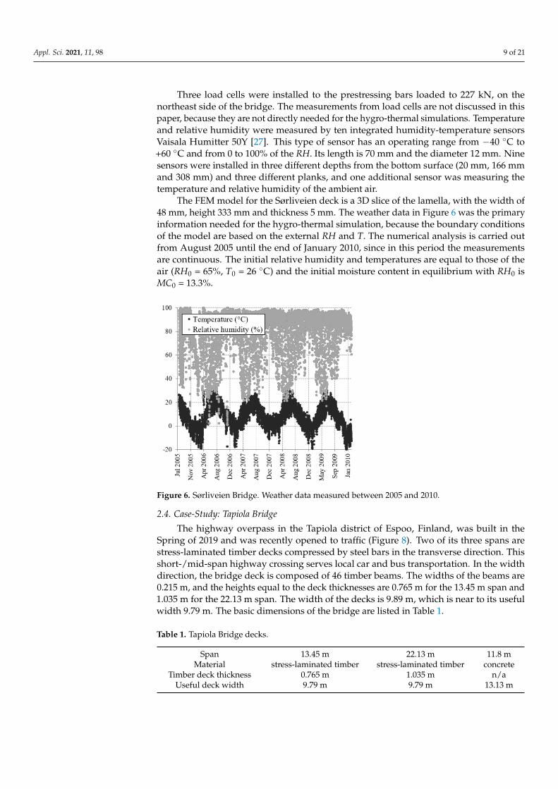
The FEM model for the Sørliveien deck is a 3D slice of the lamella, with the width of48 mm, height 333 mm and thickness 5 mm. The weather data in Figure 6 was the primaryinformation needed for the hygro-thermal simulation, because the boundary conditionsof the model are based on the external RH and T. The numerical analysis is carried outfrom August 2005 until the end of January 2010, since in this period the measurementsare continuous. The initial relative humidity and temperatures are equal to those of theair (RH0 = 65%, T0 = 26 ◦C) and the initial moisture content in equilibrium with RH0 isMC0 = 13.3%.

Figure 6. Sørliveien Bridge. Weather data measured between 2005 and 2010.

2.4. Case-Study: Tapiola Bridge

The highway overpass in the Tapiola district of Espoo, Finland, was built in theSpring of 2019 and was recently opened to traffic (Figure 8). Two of its three spans arestress-laminated timber decks compressed by steel bars in the transverse direction. Thisshort-/mid-span highway crossing serves local car and bus transportation. In the widthdirection, the bridge deck is composed of 46 timber beams. The widths of the beams are0.215 m, and the heights equal to the deck thicknesses are 0.765 m for the 13.45 m span and1.035 m for the 22.13 m span. The width of the decks is 9.89 m, which is near to its usefulwidth 9.79 m. The basic dimensions of the bridge are listed in Table 1.

Table 1. Tapiola Bridge decks.

Span 13.45 m 22.13 m 11.8 mMaterial stress-laminated timber stress-laminated timber concrete

Timber deck thickness 0.765 m 1.035 m n/aUseful deck width 9.79 m 9.79 m 13.13 m

Appl. Sci. 2021, 11, 98 10 of 21

Five integrated humidity-temperature sensors, two displacement and two force sen-sors were installed on the bridge. The displacement sensors monitor vertical and horizontalmotion, while the force sensors are measuring the tension force variation in the steel bars.In addition, the monitoring unit cabinet has two thermocouples for tracking its inside andoutside temperature. The sensors are described in Table 2. Figure 7 shows the locationsof the sensors. More details on the sensor locations are provided in Figures A1 and A2 ofAppendix B.

Table 2. The installed sensors in Tapiola Bridge deck.

No. ID Sensor Type Model

1 KC1 Humidity and temperature HMP110 [27]2 KC2 Humidity and temperature HMP1103 KC3 Humidity and temperature HMP1104 KC4 Humidity and temperature HMP1105 KC5 Humidity and temperature HMP110

6 V1 Force C6A [28]7 V2 Force C6A

8 D1x Slab longitudinaldisplacement ELPC100 linear potentiometer of OPKON [29]

9 D2y Slab vertical displacement ELPC 100 linear potentiometer of OPKON

Figure 7. Tapiola Bridge. Photos of the sensor locations: (a) from the bottom; (b): from the lateral side. See the details aboutthe locations of all sensors in Appendix B.

The sensors have wired connections to the monitoring unit. The unit itself is placed inthe metal cabinet on the abutment of the bridge and it is connected to the electric grid andthe internet. The devices and programmes of the unit are shown in Table 3.

Before the installation, the sensors were tested in the humidity-temperature controlledrooms at VTT Technical Research Centre of Finland Ltd (VTT). Only the temperaturesensors (thermocouples), located inside and outside of the measurement enclosure werenot calibrated, because they have lower precision requirements.

Appl. Sci. 2021, 11, 98 11 of 21

Figure 8. Tapiola Bridge. (a) The scheme of the transverse prestressed glulam wooden slabs of the bridge where T2, T3 andT4 indicate the support, reproduced from [30] with permission from VTT publications. Detail A is shown in Appendix B.(b) A picture with the view of the bridge.

Table 3. The devices and software of the monitoring unit.

Industrial PC: Advantech [31]Measurement software: Labview [32]Remote desktop software: DWAgent [33]Data acquisition chassis: NI cDAQ-9174 [32]Data acquisition devices: NI 9211 (thermocouple) [32]

NI 9205 (temperature, moisture) [32]NI 9237 (Force) [33]

Power supply: Quint Power [34]Enclosure internal thermostatEnclosure heaterThermocouples

The force sensor calibration was performed with the test rig of VTT, and a calibrationfactor of 0.95 was found. The current measurement system is able to record the relative forceshift/change of the pre-tension bars. Displacement sensors were not explicitly calibrated,instead the manufacturer’s instructions and precision requirements are followed [29].

The deck is protected with Valtti colour, an oil-based wood strain produced byTikkurila [35]. According to the producer, this paint exhibits a low vapour resistance.

The FEM model for the deck is a 3D slice having a width of 107.5 mm (half of thelamination), height 1035 mm and thickness 5 mm. The numerical analysis of the TapiolaBridge deck starts at the end of the construction time (April 2019) until October 2020, seethe weather data in Figure 9, while the sensor-based monitoring started later (October2019) and is on-going. The earlier starting of the numerical analysis demonstrates that thenumerical models can assist the monitoring by predicting the hygro-thermal response of theSLTD also in the absence of measurements. The initial relative humidity and temperaturesare equal to those of the air (RH0 = 65%, T0 = 0.85 ◦C) and the initial moisture content inequilibrium with RH0 is MC0 = 15.3%.

Appl. Sci. 2021, 11, 98 12 of 21

Figure 9. Tapiola Bridge. Weather data measured between 2019 and 2020.

3. Results3.1. Hygro-Thermal Response of the Deck of Sørliveien Bridge

The outputs of the finite element model are the temperature, the moisture content andthe vapour pressure in the wood material.

Since the RH and T in wood were measured directly by the monitoring system,reference results for the validation of the numerical model were available from all of thenine integrated humidity-temperature sensors installed in the wood lamellas. For thepurpose of investigation of MCs and moisture gradients near the surface of untreated woodexposed to the external climate, data measured at 20 mm from the bottom surface wereselected for comparison with the numerical results.

Figure 10 shows the comparisons in terms of vapour pressures between the measuredand numerical data. The directly measured RH in wood was multiplied by the saturatedvapour pressure by using the same Equation (9) adopted for the numerical model. Figure 11presents the comparison between measured and numerical values of temperatures. Theresults of the FEM calculation show a good correlation to the yearly variation of themonitored temperatures and measurement-based vapour pressures.

Figure 10. Sørliveien Bridge. Comparison between measurement-based and numerical vapour pressures in wood at 20 mmfrom the bottom surface.

Appl. Sci. 2021, 11, 98 13 of 21

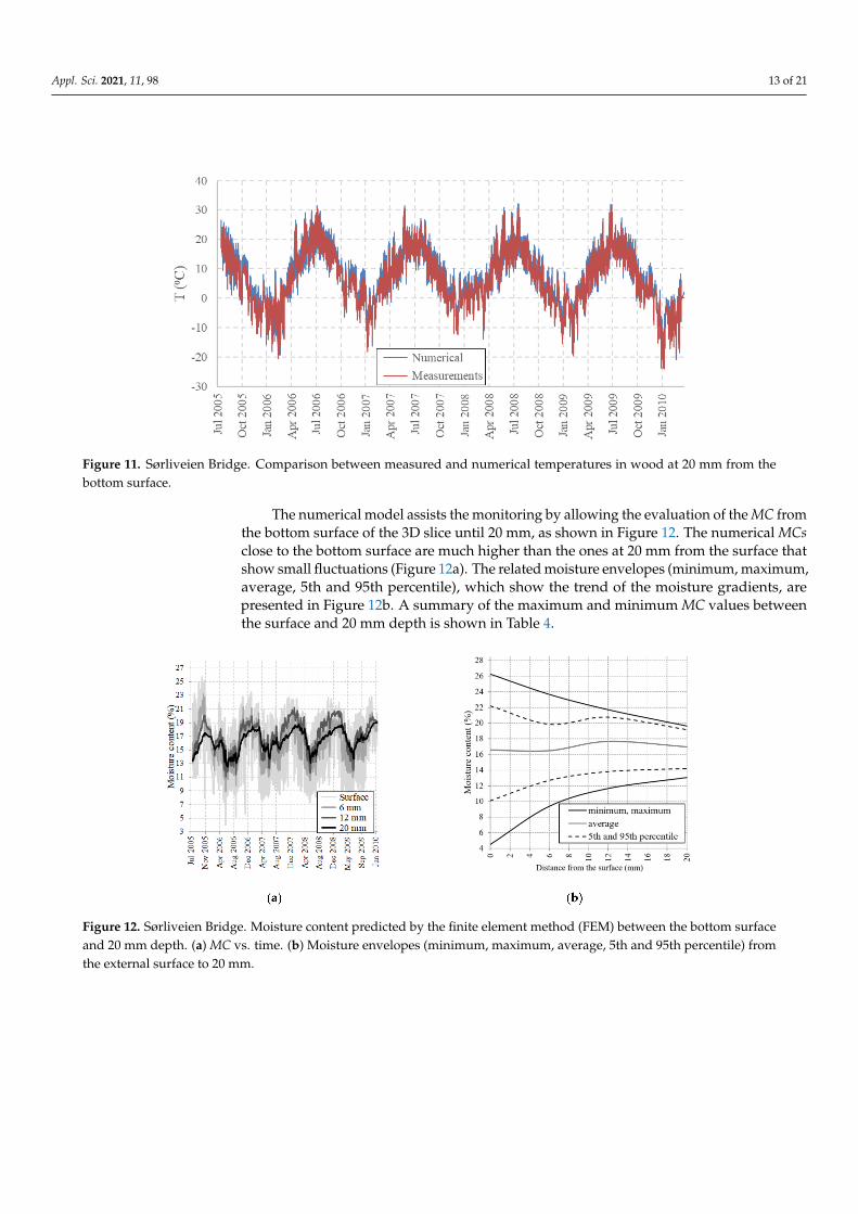
Figure 11. Sørliveien Bridge. Comparison between measured and numerical temperatures in wood at 20 mm from thebottom surface.

The numerical model assists the monitoring by allowing the evaluation of the MC fromthe bottom surface of the 3D slice until 20 mm, as shown in Figure 12. The numerical MCsclose to the bottom surface are much higher than the ones at 20 mm from the surface thatshow small fluctuations (Figure 12a). The related moisture envelopes (minimum, maximum,average, 5th and 95th percentile), which show the trend of the moisture gradients, arepresented in Figure 12b. A summary of the maximum and minimum MC values betweenthe surface and 20 mm depth is shown in Table 4.

Figure 12. Sørliveien Bridge. Moisture content predicted by the finite element method (FEM) between the bottom surfaceand 20 mm depth. (a) MC vs. time. (b) Moisture envelopes (minimum, maximum, average, 5th and 95th percentile) fromthe external surface to 20 mm.

Appl. Sci. 2021, 11, 98 14 of 21

Table 4. Sørliveien Bridge. Numerical moisture content (MC) peaks at the bottom surface and 6, 12,20 mm from the surface.

Distance fromBottom (mm) Max MC (%) Date Min MC (%) Date

0 25.8 31 October 2005 4 26 May 20066 23.2 12 November 2005 8.9 27 May 2006

12 21.2 19 January 2008 11.1 28 May 200620 19 26 February 2010 12.5 7 June 2006

3.2. Hygro-Thermal Response of the Deck of Tapiola Bridge

In this case-study, in this case-study, the results of the FEM analysis are in goodagreement with the yearly variation of the temperatures and vapour pressures monitoredat 60 mm from the bottom surface in sensors KC1 and KC2 (Figures 13 and 14). The largertemperatures measured in KC1 are because this sensor is located on the bridge side exposedto sun while KC2 is in the shadow. Since the model does not include the effect of solarradiation, the better comparison is with the data provided by sensor KC2 that is installedfrom the bottom of the deck.

Figure 13. Tapiola Bridge. Comparison between numerical temperatures in wood and measurements in sensors KC1 andKC2 at 60 mm from the surface.

The MC history at 60 mm from the bottom surface shows very small daily fluctuationswhile the numerical results closer to the surface are larger (Figure 15a). Figure 15b showsthe minimum and maximum moisture envelopes during the monitoring time, as well asthe 5th and 95th percentile from the external bottom surface to 60 mm depth. For thisthick deck, a summary of the maximum and minimum MC values between the surface and400 mm depth is shown in Table 5.

Appl. Sci. 2021, 11, 98 15 of 21

Figure 14. Tapiola Bridge. Comparison between numerical vapour pressures in wood and measurements in sensor KC2 at60 mm from the bottom surface. In red the vapour pressure measurements in sensor KC1 at 60 mm from the lateral sideexposed to the afternoon sun.

Figure 15. Tapiola Bridge. (a) Moisture contents from the external surface of the deck until 60 mm depth. (b) Moistureenvelopes (minimum, maximum, average, 5th and 95th percentile) from the external surface to 60 mm.

Table 5. Tapiola Bridge. Numerical MC peaks at the bottom surface and 20, 60, 200 and 400 mm fromthe surface.

Distance fromBottom (mm) Max MC (%) Date Min MC (%) Date

0 23.1 25 December 2019 10.8 25 June 202020 19 15 March 2020 14.1 8 August 201960 16.7 19 April 2020 14.9 10 August 2019

200 15.4 30 September 2020 15.3 18 December 2019400 15.3 12 April 2019 15.3 25 June 2020

Appl. Sci. 2021, 11, 98 16 of 21

4. Discussion

The combination of the sensor-based monitoring and numerical model presented inthe previous sections, allowed analysing the hygro-thermal response of the uncoated SLTDof Sørliveien Bridge in Norway and the thick painted SLTD of Tapiola Bridge in Finland.In addition to the temperature T and vapour pressure pv, the numerical model was able toprovide quantitative values of the moisture content MC and the moisture gradients trendsclose to the surface that could be responsible of surface cracks, as shown in earlier worksfor large glulam beams of timber bridges [10–12] and in a research on the monitoring oflarge span timber structures [36]. In particular, we analysed the bottom part of decks whichare sheltered from rain but subjected to both the continuously variable air humidity andtemperature.

The uncoated deck of Sørliveien Bridge in Norway was analysed as a first case-study,and showed a relatively stable moisture behaviour after one year from the bridge erection.The main findings are listed below:

• Referring to Table 4, the MC values on the bottom surface span in a range between4% (reached at the beginning of summer 2006) and 25.8% (autumn 2005), are highestduring the first year of the analysis and more stable during the successive years(Figure 12). The minimum and maximum MC values at 20 mm from the bottomsurface are 12.5% at the beginning of the summer 2006, and 19% at the end of winter2010. The results show that no significant changes of the average moisture contentwould be expected after the first year of the bridge service life, i.e., from June 2006 toJanuary 2010.

• High levels of MC over 20% were found only on the exposed surface at the bottomdeck and in locations very close to this surface (Figure 12). These MC levels could bealso critical for the wood durability [3], however the decay is a major problem mainlyin the presence of liquid water due e.g., to rain and eventual water traps, and thesecases were not investigated in the present work.

The painted and thick deck of Tapiola Bridge was analysed as second case-study,starting from an earlier stage after construction. The main findings are the following:

• Referring to Table 5, the moisture contents on the bottom surface varies between10.8%, reached at the beginning of the summer, and 23% at the beginning of thewinter. In the internal locations, the maximum and minimum moisture contents arereached earlier depending on the maximum moisture penetration depth, which isabout 200 mm (see Table 5). The maximum and minimum MC values in the locationof the humidity-temperature sensor at 60 mm from the bottom surface are 16.7%, atthe beginning of spring, and 14.9% at the end of summer.

• High levels of MC (i.e., >20%) were found only on the exposed bottom surface and inlocations very close to this surface. Compared to the MCs of Sørliveien Bridge, thepeaks remained below 23% (Figure 15). This is because Tapiola Bridge is protected,even if the used paint has low vapour resistance (see Table A3 of Appendix A).

The following observations are based on the comparisons between the two case-studies:

• Considering the MC results of Sørliveien Bridge, it could be estimated that also forTapiola Bridge the average values of MC will not change significantly during thesuccessive years.

• The envelope curves shown in Figure 15b indicate similar levels of moisture gradientsclose to the surface as those of the Sørliveien Bridge’s deck (Figure 12b). The averageMCs are around 16% up to 20 mm depth, and remain at an almost constant level upuntil 60 mm depth in Tapiola Bridge’s deck. Previous hygro-thermal models of SLTDs,based on single-phase moisture transport, found cupping deformations of around16 mm and steel bar force losses of around 33% at these MC levels after 15 months [9].

The displacements and forces measured in the other sensors of the two monitoringsystems can be simulated in future work by integrating the hygro-thermal analysis with amechanical model for wood as in [9,12].

Appl. Sci. 2021, 11, 98 17 of 21

The embedded sensors and computational unit allow further expansion of the Internetof Things (IoT) network in order to efficiently exchange the monitoring data with passingvehicles and stationary objects of the road infrastructure. Moreover, combined with theresults of the FEM simulation, the system can provide a comprehensive understanding ofthe bridge deck conditions in real time.

5. Conclusions

This paper proposed the use of an advanced multi-phase numerical model for woodbelow the fibre saturation point, previously introduced by some of the authors, to assist themonitoring of stress laminated timber decks by integrated humidity-temperature sensors.

The hygro-thermal simulation of a representative deck volume under Northern Euro-pean climates supplements the sensor-based data. The simulation provides the distributionof the moisture content below the FSP, the temperature and the vapour pressure in thestudied volume and allows to draw conclusions about the hygro-thermal response of thedeck. However, the model does not include the effect of solar radiation and this is a taskfor future research. The modelling of the protective asphalt layer is also a topic for futurework. The two analysed case-studies are sheltered from rain. To consider the effects ofrain and possible water traps, the current model needs to be extended by introducing thevariable concentration of free water in the lumens.

In future coupled hygro-thermo-mechanical models for SLTDs, the accurate evaluationof moisture contents is important for the prediction of moisture induced stresses which areresponsible for surface cracking, cupping deformations and losses of the pre-stress force insteel bars.

The proposed method can be used to assist the monitoring techniques under Nordicclimates contributing to maintenance cost reduction of timber bridge decks. FEM-assistedmonitoring of bridges has a great potential to decrease the cost of instrumentation andincrease safety. It can predict possible damages and communicate the results to otherinfrastructure components.

Author Contributions: Conceptualization, S.F., P.H., L.F.; methodology, S.F., P.H., H.B., K.K.; soft-ware, S.F., P.H., K.K.; validation, S.F., P.H., A.K.; formal analysis, S.F., P.H.; investigation, H.B., K.K.;resources, T.T.; data curation, P.H., K.K., H.B.; writing—original draft preparation, S.F., P.H.; writing—review and editing, P.H., L.F., T.T.; visualization, P.H., A.K.; supervision, S.F.; project administration,S.F.; funding acquisition, S.F., T.T. All authors have read and agreed to the published version ofthe manuscript.

Funding: This research was funded by WoodWisdom-Net project “Durable Timber Bridges” andby project “Delivering Fingertip Knowledge to Enable Service Life Performance Specification ofWood—Click Design”, which is supported under the umbrella of ERA-NET Cofund ForestValue bythe Ministry of the Environment of Finland. ForestValue has received funding from the EuropeanUnion’s Horizon 2020 research and innovation program. The Finnish Transport Infrastructure Agency(Väylävirasto) is a co-funder of the Click Design project.

Informed Consent Statement: Informed consent was obtained from all subjects involved in the study.

Data Availability Statement: The data presented in this study are available on request from thecorresponding author. The data are not publicly available due to the agreements with the fund-ing projects.

Acknowledgments: The authors wish to thank the Norwegian Public Road Administration forproviding the monitoring data of Sørliveien Bridge. The Finnish Transport Infrastructure Agency(Väylävirasto) and the City of Espoo is acknowledged for supporting the monitoring of the TapiolaBridge. The authors would like to warmly thank VTT colleagues Jukka Mäkinen, Mikko Kallio, KalleRaunio, Pekka Halonen, Kari Korhonen for taking care of the on-going monitoring of Tapiola Bridge.

Conflicts of Interest: The authors declare no conflict of interest. Co-funder Väylävirasto (T.T.)participated in the interpretation of data, writing of the manuscript and in the decision to publishthe results.

Appl. Sci. 2021, 11, 98 18 of 21

Appendix A

Table A1. Material parameters for the multi-Fickian model (all references can be found in [11]).

Water vapour diffusion tensor

Dv = ξv

(2.31·10−5

(patm

patm+ pv

)(T

273

)1.81) (

m2s−1)• Atmospheric pressure patm = 101325 Pa• Vapour pressure pv = cvRT/(ϕMH2O)

• Gas constant R = 8.314(

Jmol−1K−1)

• Molecular mass of water MH2O = 18.02× 10−3(

kgmol−1)

Components of reduction factor ξvξvL = 0.9 longitudinalξvT = 0.12 transverse (*)

Bound water diffusion tensorDb = D0exp

(− Eb

RT

) (m2s−1)

• Activation energy of bound water diffusion

• Eb = (38.5− 29MC)·103(

Jmol−1)

Components of diagonal tensor D0D0L = 17.5·10−6 (m2s−1) longitudinalD0T = 7·10−6 (m2s−1) transverse

Thermal conductivity tensor

K = ξH(G(0.2 + 0.38MC) + 0.024)(

Wm−1K−1)

• Specific gravity of wood G = 0.693G0/(0.653 + MC)• G0 = $0/$0w = dry wood density/water density

Components of reduction factor ξHξHL = 2.5 longitudinalξHT = 1 transverse

Specific heat cw = 0.0011T+MC−0.03231+MC

(Jkg−1K−1

)Wood density $ = G(1 + MC)$w

(kgm−3

)Enthalpy of bound water

hb = − 7.8955·105 − 4.476206·102T + 2.274399·10T2 − 4.9553577·10−2 T3 + 4.041035·10−5T4(

Jkg−1)

Enthalpy of water vapour

hv = 1.891879× 106 + 2.56352× 103T − 1.2360577T2(

Jkg−1)

Sorption reaction rate function

Hc =

C1exp

(−C2

(cbcbl

)C3)

+ C4 cb < cbl

C1exp(− C2

(2− cb

cbl

)C3)

+ C4 cb > cbl

ConstantsC1 = 3.8·10−4(s−1)C2 = c21exp(c22RH) + c23exp(c24RH)C3 = 80.0C4 = 5.94·10−7(s−1)c21 = 3.579c22 = 2.21c23 = 1.591·10−3

c24 = 14.98

Anderson–McCarthy model for sorption isotherms

MCbl,α = − 1f2α

ln(

ln( 1RH )

f1α

), α ∈ {a, d}

• a and d refer to adsorption and desorption

• fiα =n∑

j=0bijαT j, i ∈ {1, 2}

See Table A2

Permeances of the painted wood referred to wood temperature and air temperature:kw

v = 11

kw+ 1

kp

RTMH2O

, kav = 1

1kw

+ 1kp

RTa

MH2O

Thermal emission:kT = 20 [W m−2 K−1]

See Table A3

(*) selected in this paper.

Appl. Sci. 2021, 11, 98 19 of 21

Table A2. Shape parameters for the temperature dependent adsorption and desorption functions.

α n b10α[-]

b11α[K−1]

b20α[-]

b21α[K−1]

a 1 7.719 −0.011 5.079 0.046d 1 9.739 −0.017 −13.419 0.100

Table A3. Permeances of weak paint and uncoated wood.

Paint Permeance[kg/m2 s Pa]

weak paint 4.0 × 10−9

uncoated wood 5.0 × 10−9

Appendix B

Figure A1. The locations of sensors in the side of the south-west corner of Slab A in the vicinity ofthe support T3 (see Figure 8a).

Appl. Sci. 2021, 11, x FOR PEER REVIEW 19 of 21

Table A2. Shape parameters for the temperature dependent adsorption and desorption functions.

α n b10α [-]

b11α [K−1]

b20α [-]

b21α [K−1]

a 1 7.719 −0.011 5.079 0.046 d 1 9.739 −0.017 −13.419 0.100

Table A3. Permeances of weak paint and uncoated wood.

paint Permeance [kg/m2 s Pa]

weak paint 4.0 × 10−9 uncoated wood 5.0 × 10−9

Appendix B

Figure A1. The locations of sensors in the side of the south-west corner of Slab A in the vicinity of the support T3 (see Figure 7a).

(a) (b)

Figure A2. Tapiola Bridge: (a) the prestressed glulam wooden Slab A of the bridge. (b) The loca-tions of sensors in the bottom of Slab A in the vicinity of the slab’s south-west corner near the sup-port T3 (see Figure 7a).

References

627

520

850

800600

1790

1035

267500

T3(Bottom of slab A)

(Top of slab A)

KC1

KC4V1

V2

Drill hole depth: 60

Drill hole depth: 400

South (Tapiola)North (Otaniemi)

Detail A

T4 T3

22516

9890

KC2

KC3 KC5

D2y

D1x

South (Tapiola)North (Otaniemi)

(Bottom of slab A)

Detail B

KC3

KC5

D2y

D1x

(Bottom of slab A)

500 110

320

1180 1400

1730

1030

Drill hole depth: 400

South (Tapiola)

Drill hole depth: 400

KC2

Drill hole depth: 60

Detail B

T3

Figure A2. Tapiola Bridge: (a) the prestressed glulam wooden Slab A of the bridge. (b) The locations of sensors in thebottom of Slab A in the vicinity of the slab’s south-west corner near the support T3 (see Figure 8a).

Appl. Sci. 2021, 11, 98 20 of 21

References1. European Committee for Standardization. EN 1990: Eurocode: Basis of Structural Design; European Committee for Standardization:

Brussels, Belgium, 2002.2. Obataya, E. Characteristics of aged wood and Japanese traditional coating technology for wood protection. In Proceedings of

the Actes de la Journée D’étude Conserver Aujourd’hui: Les “Vieillissements” du Bois, Cité de la Musique, Paris, France, 2February 2007.

3. Brischke, C.; Meyer-Veltrup, L. Modelling timber decay caused by brown rot fungi. Mater. Struct. 2016, 49, 3281–3291. [CrossRef]4. Wacker, J. Cold Temperature Effect on Stress-Laminated Timber Bridges: A Laboratory Study; Research Paper FPL–RP–605; U.S.

Department of Agriculture, Forest Service, Forest Products Laboratory: Madison, WI, USA, 2003.5. Scharmacher, F.; Müller, A.; Brunner, M. Asphalt surfacing on timber bridges. In Proceedings of the COST-Timber Bridges,

Biel, Switzerland, 25–26 September 2014; Franke, S., Franke, B., Widmann, R., Eds.; Bern University of Applied Sciences: Bern,Switzerland, 2014.

6. Aasheim, E. Nordic timber bridge program—An overview. In Proceedings of the International Wood Engineering Conference,New Orleans, LA, USA, 21–28 October 1996; Gopu, V.K.A., Ed.; International Wood Engineering Conference: New Orleans, LA,USA, 1996.

7. Horn, H. Rapport Oppdrag Nr. 310332: Monitoring Five Timber Bridges in Norway—Results 2012; Norsk Treteknisk Institut: Oslo,Norway, 2013.

8. Ministry of the Environment, Department of the Built Environment. Wood Building Programme. Available online: https://ym.fi/en/wood-building (accessed on 14 November 2020).

9. Pousette, A.; Malo, K.; Thelandersson, S.; Fortino, S.; Salokangas, L.; Wacker, J. Durable Timber Bridges—Final Report and Guidelines;SP Report 25; Research Institutes of Sweden RISE: Skellefteå, Sweden, 2017.

10. Fortino, S.; Genoese, A.; Genoese, A.; Nunes, L.; Palma, P. Numerical modelling of the hygro-thermal response of timber bridgesduring their service life: A monitoring case-study. Constr. Build. Mater. 2013, 47, 1225–1234. [CrossRef]

11. Fortino, S.; Hradil, P.; Genoese, A.; Genoese, A.; Pousette, A. Numerical hygro-thermal analysis of coated wooden bridgemembers exposed to Northern European climates. Constr. Build. Mater. 2019, 208, 492–505. [CrossRef]

12. Fortino, S.; Hradil, P.; Metelli, G. Moisture-induced stresses in large glulam beams. Case study: Vihantasalmi Bridge. Wood Mater.Sci. Eng. 2019, 14, 366–380. [CrossRef]

13. Fragiacomo, M.; Fortino, S.; Tononi, D.; Usardi, I.; Toratti, T. Moisture-induced stresses perpendicular to grain in cross-sections oftimber members exposed to different climates. Eng. Struct. 2011, 33, 3071–3078. [CrossRef]

14. Niklewski, J.; Fredriksson, M. The effects of joints on the moisture behaviour of rain exposed wood: A numerical study withexperimental validation. Wood Mater. Sci. Eng. 2019, 1–11. [CrossRef]

15. Florisson, S.; Vessby, J.; Mmari, W.; Ormarsson, S. Three-dimensional orthotropic nonlinear transient moisture simulation forwood: Analysis on the effect of scanning curves and nonlinearity. Wood Sci. Technol. 2020, 54, 1197–1222. [CrossRef]

16. Krabbenhøft, K. Moisture Transport in Wood: A Study of Physical-Mathematical Models and their Numerical Implementation.Ph.D. Thesis, Technical University of Denmark, Lyngby, Denmark, 2004.

17. Frandsen, H.L. Selected Constitutive models for simulating the hygromechanical response of wood. Ph.D. Thesis, Department ofCivil Engineering Aalborg University, Aalborg, Denmark, 2007.

18. Eitelberger, J.; Hofstetter, K.; Dvinskikh, S.V. A multi-scale approach for simulation of transient moisture transport processes inwood below the fiber saturation point. Compos. Sci. Technol. 2011, 71, 1727–1738. [CrossRef]

19. Konopka, D.; Kaliske, M. Transient multi-Fickian hygro-mechanical analysis of wood. Comput. Struct. 2018, 197, 12–27. [CrossRef]20. Huc, S.; Svensson, S.; Hozjan, T. Hygro-mechanical analysis of wood subjected to constant mechanical load and varying relative

humidity. Holzforschung 2018, 72, 863–870. [CrossRef]21. Autengruber, M.; Lukacevic, M.; Füssl, J. Finite-element-based moisture transport model for wood including free water above the

fiber saturation point. Int. J. Heat Mass Transf. 2020, 161, 120228:1–120228:21. [CrossRef]22. Svensson, S.; Turk, G.; Hozjan, T. Predicting moisture state of timber members in a continuously varying climate. Eng. Struct.

2011, 33, 3064–3070. [CrossRef]23. Thalla, O.; Stiros, S.C. Wind-Induced Fatigue and Asymmetric Damage in a Timber Bridge. Sensors 2018, 18, 3867. [CrossRef]

[PubMed]24. Kepp, H.; Dyken, T. Thermal cction on timber bridges temperature variation measured in the deck of 3 timber bridges in Norway.

In Proceedings of the International Conference Timber Bridges (ICTB2010), Lillehammer, Norway, 12–15 September 2010; Malo,K.A., Kleppe, O., Dyken, T., Eds.; Tapir Academic Press: Trondheim, Norway, 2010.

25. Dyken, T.; Kepp, H. Monitoring the moisture content of timber bridges. In Proceedings of the International Conference TimberBridges (ICTB2010), Lillehammer, Norway, 12–15 September 2010; Malo, K.A., Kleppe, O., Dyken, T., Eds.; Tapir Academic Press:Trondheim, Norway, 2010.

26. Frandsen, H.L. Modelling of Moisture Transport in Wood: State of the Art and Analytic Discussion, 2nd ed.; Aalborg University:Aalborg, Denmark, 2005.

27. Vaisala Oyj Home Page. Available online: https://www.vaisala.com/ (accessed on 24 November 2020).28. Hottinger Brüel & Kjaer GmbH Home Page. Available online: https://www.hbm.com/ (accessed on 24 November 2020).

Appl. Sci. 2021, 11, 98 21 of 21

29. Opkon Optik Elektronik Kontrol San. Tic. Ltd. Sti Home Page. Available online: https://www.opkon.com.tr/ (accessed on 24November 2020).

30. Koski, K. Instrumentation of Tapiolantien Risteyssilta (Bridge); Research Report VTT-R-00837-19; Technical Research Centre ofFinland: Espoo, Finland, 2019.

31. Advantech, Co., Ltd. Home Page. Available online: https://www.advantech.com/ (accessed on 24 November 2020).32. National Instruments. Home Page. Available online: http://www.ni.com/ (accessed on 24 November 2020).33. DWS remote Control. Home Page. Available online: https://www.dwservice.net/ (accessed on 24 November 2020).34. Phoenix Contact. Home Page. Available online: https://www.phoenixcontact.com/ (accessed on 24 November 2020).35. Tikkurila Valtti Color Safety Data Sheet. Available online: https://tikkurila.com/sites/default/files/valtti-color-sds-en.pdf

(accessed on 14 November 2020).36. Dietsch, P.; Gamper, A.; Merk, M.; Winter, S. Monitoring building climate and timber moisture gradient in large-span timber

structures. J. Civil. Struct. Health Monit. 2015, 5, 153–165. [CrossRef]