gully mapping using remote sensing: case study in kwazulu
TRANSCRIPT
Gully Mapping using Remote Sensing:
Case Study in KwaZulu-Natal, South
Africa
by
Kanyadzo Taruvinga
A thesis
presented to the University of Waterloo
in fulfillment of the
thesis requirement for the degree of
Master of Environmental Studies
in
Geography
Waterloo, Ontario, Canada, 2008
© Kanyadzo Taruvinga 2008

ii
AUTHOR'S DECLARATION
I hereby declare that I am the sole author of this thesis. This is a true copy of the thesis, including any
required final revisions, as accepted by my examiners. I understand that my thesis may be made
electronically available to the public.

iii
Abstract
At present one of the challenges of soil erosion research in South Africa is the limited information on
the location of gullies. This is because traditional techniques for mapping erosion which consists of
the manual digitization of gullies from air photos or satellite imagery, is limited to expert knowledge
and is very time consuming and costly at a regional scale (50-10000km²). Developing a robust,
reliable and accurate means of mapping gullies is a current focus for the Institute for Soil, Climate
and Water Conservation (ISCW) of the Agricultural Research Council (ARC) of South Africa. The
following thesis attempted to answer the question whether “medium resolution multi-spectral satellite
observations, such as Landsat TM, combined with information extraction techniques, such as
Vegetation Indices and multispectral classification algorithms, can provide a semi-automatic method
of mapping gullies and to what level of accuracy?”.
More specifically, this thesis investigated the utility of three Landsat TM-derived Vegetation Index
(VI) techniques and three classification techniques based on their level of accuracy compared to
traditional gully mapping methods applied to SPOT 5 panchromatic imagery at selected scales. The
chosen study area was located in the province of KwaZulu-Natal (KZN) South Africa, which is
considered to be the province most vulnerable to considerable levels of water erosion, mainly gully
erosion. Analysis of the vegetation indices found that Normalized Difference Vegetation Index
(NDVI) produced the highest accuracy for mapping gullies at the sub-catchment level while
Transformed Soil Adjusted Vegetation Index (TSAVI) was successful at mapping gullies at the
continuous gully level. Mapping of gullies using classification algorithms highlighted the spectral
complexity of gullies and the challenges faced when trying to identify them from the surrounding
areas. The Support Vector Machine (SVM) classification algorithm produced the highest accuracy for
mapping gullies in all the tested scales and was the recommended approach to gully mapping using
remote sensing.

iv
Acknowledgements
The successful completion of this thesis is due to all the help and support I have received from many
different people, both in the collection and processing of all the data used in this thesis and in the
writing and editing of the final product. I would like to first express my sincerest appreciation to the
people at the Agricultural Research Council (ARC), Mr. and Mrs. Grundling and Mr. Jay Le Roux,
for creating this wonderful research opportunity, supporting me in every way during my time in South
Africa and assisting in my field work. I would also like to thank my colleague Miss Holly Waite for
her amazing support in brainstorming ideas, staying up with me all those late nights, proof reading
my material and being the strongest shoulder to cry on. Another special thanks is given to my family
and friends for being so supportive through the duration of my thesis. Last but defiantly not least I
would also like to thank Dr. Richard Kelly and Dr. Jonathan Price from the University of Waterloo
for their help and guidance in my research, and providing me with exceptional advice.

v
Table of Contents
Chapter 1 Introduction............................................................................................................................ 1
1.1 Overview ...................................................................................................................................... 1
1.2 Thesis Outline............................................................................................................................... 4
Chapter 2 Research Context ................................................................................................................... 5
2.1 Geomorphology Background of Gully Erosion............................................................................ 5
2.2 Traditional Gully Mapping Methods.......................................................................................... 11
2.3 Gully Mapping Using Remote Sensing...................................................................................... 14
2.4 Specific Objectives..................................................................................................................... 38
Chapter 3 Site Description.................................................................................................................... 40
3.1 Location...................................................................................................................................... 40
3.2 Climate ....................................................................................................................................... 41
3.3 Vegetation .................................................................................................................................. 42
3.4 Geology and Soils ...................................................................................................................... 42
3.5 Land Use..................................................................................................................................... 43
3.6 Erosion Status............................................................................................................................. 44
3.7 Summary .................................................................................................................................... 44
Chapter 4 Methodology........................................................................................................................ 46
4.1 Preprocessing.............................................................................................................................. 46
4.2 Mapping Methodology ............................................................................................................... 50
Chapter 5 Results.................................................................................................................................. 61
5.1 Vegetation Indices ...................................................................................................................... 61
5.2 Gully Mapping Results from Multi-spectral Classification Techniques .................................... 72
5.3 Summary of Results ................................................................................................................... 82
Chapter 6 Discussion............................................................................................................................ 84
6.1 Issue of Detectability.................................................................................................................. 84
6.2 Possible Explanations for Low Accuracy of Maps .................................................................... 86
Chapter 7 Conclusions and Recommendations .................................................................................... 88
References ............................................................................................................................................ 91
Appendix A………………………………………………………………………………………….105
Appendix B…………………………………………………………………………………………..106
Appendix C…………………………………………………………………………………………..107

vi
Appendix D…………………………………………………………………………………………108
Appendix E………………………………………………………………………………………….109
vii
List of Figures
Figure 2-1 An example of different drainage patterns. a) dendritic, (b) parallel, (c) radial, (d)
centrifugal, (e) Centripetal, (f) distributary, (g) angular, (h) trellis, (i) annular (adapted from
Twidale, 2004)................................................................................................................................ 6
Figure 2-2 Gully development by surface and subsurface soil erosion modified from (Summer and
Meiklejohn, 2000) .......................................................................................................................... 8
Figure 2-3 Stages of gully development, from discontinuous gullies to a continuous gully, extracted
from Leopold et al. (1964). ............................................................................................................ 9
Figure 2-4 Spectral responses of clay and sandy soils from Hoffer and Johannsen (1969) ................. 20
Figure 2-5 An example of soil variability within a gully that has incised into a thin colluvium layer
overlying mudstones and subordinate sandstones. Left are four cross-sections of the gully system
at different points. Right is an aerial view of the gully system with graphs displaying elevation
change in the landscape (A,B,C,and D). Modified from (Dardis, 1991)...................................... 21
Figure 2-6 Spectral curves of selected regions of interest (Landsat TM),............................................ 23
Figure 2-7 The classification process (modified from Schowengerdt, 2002) ...................................... 27
Figure 2-8 Displays class A and class B plotted in an x-y feature space, with hypothetical probability
contours and means. Modified from Mather (2004)..................................................................... 29
Figure 2-9 The kernel maps the training samples into a higher dimensional feature space via a
nonlinear function and constructs a separating hyperplane with maximum margins. Modified
from Camps-Valls et al. (2004).................................................................................................... 32
Figure 2-10 a) SMV separating linearly separable classes. In separating classes that are not linearly
separable b) the SVMs task is to find the cost separated marginal hyperplanes that minimize the
slack variables and maximize the margins. .................................................................................. 33
Figure 2-11 A simple accuracy assessment illustrations ...................................................................... 37
Figure 3-1 Location of study area in South Africa (spatial data source: ARC, (2007))....................... 40
Figure 3-2 Location of study region within Buffalo River sub-catchment (spatial data source: rivers
(DWAF, 2007) towns and catchment (ARC, 2007)).................................................................... 41
Figure 3-3 Lithostratigraphy of the Karoo Supergroups present in the study area............................... 43
Figure 4-1 Methodology flow diagram ................................................................................................ 46
Figure 4-2 Left: Map illustrating the sub-catchment level of the study area and the Landsat TM
track/row. Right: The locations of the chosen subsets within the selected preprocessed Landsat

viii
TM sub-catchment subset. Label ‘A’ is the continuous gully system, and label ‘B’ is the
discontinuous gullies.................................................................................................................... 49
Figure 4-3 Flow diagram of the "Ground Truth" gully maps .............................................................. 51
Figure 4-4 A1 and B1 are the digitized gullies, in red solid line, on a true colour composite of SPOT
5. A2 and B2 are the gully maps created for the discontinuous and continuous subsets
respectively. ................................................................................................................................. 53
Figure 4-5 A NIR/Red 2-D scatter plot of 200 bare soil pixels. The straight solid line corresponds to
the soil line for this particular data set. ........................................................................................ 54
Figure 4-6 Flow diagram of Vegetation Index gully maps .................................................................. 56
Figure 4-7 Flow diagram of classification gully maps......................................................................... 60
Figure 5-1 Spatial profile of NDVI, SAVI and TSAVI values across different land cover types in the
study area ..................................................................................................................................... 62
Figure 5-2Top image is a false colour composite of the continuous gully subset. Bottom (left to right)
are the NDVI, SAVI and TSAVI results for the continuous gully subset. .................................. 63
Figure 5-3 Spatial profile of NDVI, SAVI, TSAVI values across a gully........................................... 64
Figure 5-4 Spatial profiles of VI values across transects along a continuous gully............................. 65
Figure 5-5 A graph of the tested upper thresholds for each vegetation index ..................................... 67
Figure 5-6 VI continuous gully map with kappa statistic results......................................................... 67
Figure 5-7 VI discontinuous gully map with VI kappa statistic results ............................................... 68
Figure 5-8 Kappa statistics graph comparing the VI results for each gully subset .............................. 69
Figure 5-9 Classification gully maps with kappa statistic results ........................................................ 75
Figure 5-10 Classification kappa statistic results for mapping gullies in each subset ........................ 76
Figure 5-11 The Gully and Non Gully training data in a five band feature space ............................... 77
Figure 5-12 MLC and MDC classification illustration of a hypothetical classification ...................... 79
Figure 6-1 Right: Spectrally similar features that were mapped as gullies. Left: TSAVI gully map and
right is the ground truth gully map............................................................................................... 85
Figure 6-2 The location where gullies were not identified using NDVI (A), SAVI (B) and TSAVI (C);
false colour composite (D) with red indicating vegetation and light blue indicating bare soil; the
purple and light blue areas in A, B and C are the errors of omission and commission. .............. 86

ix
List of Tables
Table 2-1 Imagery characteristics ........................................................................................................ 15
Table 4-1 Test 1: Training data sizes with a large non gully class size................................................ 58
Table 4-2 Test 2: Training data sizes with a small non gully class size............................................... 58
Table 5-1 Tested upper VI thresholds that produced the highest kappa statistic for gully mapping in
the continuous gully subset .......................................................................................................... 66
Table 5-2 VI kappa statistic results for the Sub-catchment gully map................................................. 68
Table 5-3 VI kappa statistic results for gully mapping in each subset ................................................. 69
Table 5-4 Classification kappa statistics results using different training data sizes............................. 73
Table 5-5 Classification kappa statistics results with selected PCA bands .......................................... 74
Table 5-6 Classification kappa statistics results for mapping gullies in subsets .................................. 76
Table 5-7 Classification kappa statistics results with SPOT 5 ............................................................. 76
Table 5-8Kappa Statistic Results Summary ......................................................................................... 83

x
List of Equations
(2-1) ..................................................................................................................................................... 24
(2-2) ..................................................................................................................................................... 25
(2-3) ..................................................................................................................................................... 25
(2-4) ..................................................................................................................................................... 26
(2-5) ..................................................................................................................................................... 28
(2-6) ..................................................................................................................................................... 30
(2-7) ..................................................................................................................................................... 35
(2-8) ..................................................................................................................................................... 35
(2-9) ..................................................................................................................................................... 35
(2-10) ................................................................................................................................................... 36
(4-1) ..................................................................................................................................................... 53
(4-2) ..................................................................................................................................................... 54
(4-3) ..................................................................................................................................................... 55

xi
List of Abbreviations
ARC - Agricultural Research Council
AVIRIS - Airborne Visible and Infrared Imaging
DN – Digital number
DWAF - Department of Water, Agriculture and Forestry
EM – Electromagnetic
ERU – Erosion Response Unit
ESM - Erosion Susceptibility Map
ETM+ - Enhanced Thematic Mapper
GIS - Geographic Information System
HRVIR - High Resolution Visible Infrared
HRV - High Resolution Visible
IR – Infrared
ISCW - Soil, Climate and Water Conservation
KZN - KwaZulu-Natal
MDC - Mahalanobis Distance Classifier
MLC - Maximum Likelihood Classifier
MSS – Multi-spectral Scanner
NDVI - Normalized Vegetation Index
NIR – Near infrared
PCA – Principle Component Analysis
PWEM - Predicted Water Erosion Map
RUSLE - Revised Universal Soil Loss Equation
SAVI – Soil Adjusted Vegetation Index
SLEMSA Soil Loss Estimator for Southern Africa
SPOT - Systeme Pour l'Observation de la
SVM - Support Vector Machine
TM - Thematic Mapper
TSAVI - Transformed Soil Adjusted Vegetation Index
USLE - Universal Soil Loss Equation


1
Chapter 1
Introduction
Soil erosion by water, particularly gully erosion, is regarded as a serious environmental
problem in South Africa where there is need for semi-automatic gully mapping methods (Le
Roux et al., 2007).
1.1 Overview
Soil erosion is a natural process caused by water, wind and ice, and is a serious land degradation
problem globally (Ritchie, 2000). Soil erosion by water is one of the most important global land
degradation problems mainly because of its negative on-site landscape effects such as loss of soil
productivity and quality (Dwivedi et al., 1997; Eswaran et al., 2001), and off-site effects such as
sedimentation of rivers, lakes and estuaries. Erosion decreases organic matter, fine grained soil
particles, water holding capacity and depth of the top soil (rooting depth) (Ritchie, 2000) and is
accelerated through anthropogenic stresses, particularly agriculture (Lal, 2001).
Soil erosion by water occurs if the combined power of the rainfall energy and overland flow exceeds
the resistance of soil to point of detachment (Hadley et al., 1985). The process involves (1)
detachment, with rainfall being the most important force of detachment (de Jong, 1994) (2)
transportation of sediment (redistribution over the landscape) by surface runoff and (3) deposition (in
depressional sites and aquatic ecosystems) of soil (Lal, 2001). The three main forms of soil erosion by
water are sheet erosion, rill erosion and gully erosion – gully erosion being the most severe. Sheet
erosion is the detachment and transportation of soil particles that occurs as a result of rainsplash and
overland flow (Garland et al., 2000). Rill erosion is the removal of soil in small channels and gully
erosion, by contrast, is the removal of soil in large channels (gullies) by concentrated runoff either on
the surface or subsurface level. From an agricultural perspective, gullies are defined as erosion
features that are too deep to be ploughed with ordinary farm equipment; although there has not been a
specific upper limit to the size of gullies, they typically range in size from 0.5m to as much as 30m
deep (Soil Science Society of America, 1996).

2
Improved mapping capabilities of gully distribution and magnitude could lead to enhancements in
agricultural production and water resource management, as well as provide more accurate hazard
maps through accurately locating severely eroded areas. Changes in the distribution and extent of
gullies play an important role in determining the location and resources required for erosion control
mitigation projects. Gully erosion maps, produced quickly and cheaply from readily-accessible
information, are a useful tool in regional planning for erosion control. Therefore, developing a robust,
reliable and accurate means of mapping gullies is a current focus for the Institute for Soil, Climate
and Water Conservation (ISCW) of the Agricultural Research Council (ARC) of South Africa (Le
Roux et al., 2007).
The gully erosion problem in South Africa is largely a product of several unfavorable natural
conditions that are characteristic of the region, primarily the low and unreliable amounts of rainfall
and soil type. The high temperatures cause rapid decomposition of organic matter which leads to a
reduction in the soils’ structural support (Laker, 2000). This is accelerated when there are episodes of
prolonged droughts followed by torrential rains because the soils are vulnerable to erosion due to lack
of vegetation cover. South Africa is characterized by highly erodible solonetzic soils (Fox and
Rowntree, 2001). These soils have very low infiltration rates. However, once saturated soil cohesion
and stability is lost leading to increased erosion (Jones and Keech, 1966). The province of KwaZulu-
Natal (KZN), with its fine-grained soils, torrential rainfall and sparse vegetation, is considered to be
the province most vulnerable to considerable levels of water erosion (Hoffman and Ashwell, 2001),
mainly gully erosion.
At present one of the challenges of soil erosion research in South Africa is the limited information on
the location of gullies (Le Roux et al., 2007; Mpumalanga, 2002). Most of the land degradation
mapping projects were conducted by recognized experts at a national scale, with little or no focus on
mapping gullies (Garland et al., 2000; Pretorius and Bezuidenhout, 1994; Pretorius, 1995). The Bare
Soil Index (BSI) map developed with Landsat TM focuses on the status of eroded areas, not
specifically delineating individual gullies (Pretorius and Bezuidenhout, 1994). The Erosion
Susceptibility Map (ESM) and Predicted Water Erosion Map (PWEM) of South Africa were
produced using an erosion model that identified areas under severe threat by water erosion but not
gully erosion specifically (Pretorius, 1995). In some areas these erosion hazard maps inaccurately
mapped the current extent of soil loss (Le Roux et al., 2007). The most recent approach was a more

3
qualitative assessment of land degradation which mapped the type and severity of soil degradation for
different land use types. This map was compiled with information gathered from 34 workshops
throughout South Africa (Garland et al., 2000; Le Roux et al., 2007) and is therefore subject to the
perspectives of the participants.
As stated by Le Roux (2007), “there exists no methodological framework, or ‘blueprint,’ to assess the
spatial distribution of soil erosion types at different regional scales in South Africa.” This is because
traditional techniques for mapping erosion which consists of the manual digitization of gullies from
air photos or satellite imagery, is limited to expert knowledge and is very time consuming and costly
at a regional scale (50-10000km²). However, multi-spectral remote sensing methods offer the
possibility of using semi-automatic mapping techniques to consistently map gullies. The following
thesis is a stepping stone for the incorporation of satellite remote sensing for mapping gullies at the
sub-catchment level in KZN, South Africa. It explores and demonstrates a standard approach for
gully mapping through addressing key issues such as expert knowledge required, time, cost and
accuracy of different remote sensing techniques.
Improving gully mapping methods by applying remote sensing is important and beneficial for erosion
control, not only in South Africa, but other regions around the world. The efficacy of efforts to
mitigate against damage caused by gully erosion rests in understanding gully erosion processes. A
robust semi-automatic procedure using remote sensing imagery to map gullies means that
geomorphologists with limited background knowledge about the location can easily and economically
create a map displaying the extent of a gully network. Furthermore, stakeholders in erosion
management require spatially explicit erosion feature maps with documented level of accuracy for
decision-making processes. The spatial and spectral resolutions of Landsat TM could be beneficial for
mapping gullies using semi-automatic methods and higher spatial resolution SPOT 5 imagery could
be used to delineate gullies using traditional methods. Therefore, the overall aim of this thesis is to
investigate the utility of Landsat TM-derived Vegetation Index (VI) techniques and three
classification techniques based on their level of accuracy compared to traditional gully mapping
methods applied to SPOT 5 panchromatic imagery in KZN. More specifically this thesis will:
1. Evaluate three vegetation indices: Normalized Difference Vegetation Index (NDVI), Soil
Adjusted Vegetation Index (SAVI) and Transformed Soil Adjusted Vegetation Index (TSAVI)
for accuracy in gully mapping;

4
2. Evaluate three supervised classification techniques: Maximum Likelihood Classifier (MLC),
Mahalanobis Distance Classifier (MDC) and Support Vector Machine (SVM) for accuracy in
gully mapping and determine if a higher spatial resolution (SPOT 5) is required to map gullies;
3. Link traditional gully mapping techniques carried out in South Africa to current remote sensing
techniques of today.
1.2 Thesis Outline
Following this section, Chapter 2 explores the literature related to gully erosion processes, traditional
and more recent techniques for mapping gullies and reviews the use of remote sensing methods for
mapping gullies in South Africa. In Chapter 3, details concerning the physical setting and site
description of the gully erosion study site are given. In Chapter 4, a description of the data collection
and processing methods are examined. In Chapter 5 the result of the analysis of the vegetation indices
and classification methods for mapping gullies is provided. Chapter 6 is a discussion of some of the
limitations of the study and finally in Chapter 7, the conclusions, and recommendations for future
research are discussed.

5
Chapter 2
Research Context
2.1 Geomorphology Background of Gully Erosion
This thesis attempts to bridge traditional gully mapping methods with current remote sensing
techniques. To do so, four fundamental questions were adapted from Klimaszewski (1982) and can be
applied to the spatial variability of gullies and the status of gullies in their evolution: (i) How are
gullies characterized morphologically (appearance, shape and past characterization)? (ii) How can
gullies be characterized by their morphometry (dimensions and geometry)? (iii) What is a gully
morphogenesis (origin and development)? and (iv) How are gully morphodynamics characterized
(interaction of a gully and the erosion controlling factor)? These questions are addressed in the
following sub-sections with specific relevance for gully erosion in South Africa.
2.1.1 Morphology: Gully Characteristics
Successful mapping depends on knowing the characteristics of a gully, and using that information to
define the appropriate mapping technique (King, 2002). Gullies have been characterized by a number
of different criteria. The Food and Agriculture Organization (FAO) (1965) and Hudson (1985)
described gullies simply as geomorphic features that do not allow for normal ploughing. The shape of
gully cross-sections and soil material in which a gully develop have also been used to characterize
gullies, with V- and U-shaped gully cross-sections subdivided according to the type of sedimentary
material present (Imeson and Kwaad, 1980). Morgan (1979) gave a more landscape-based approach
defining gullies as “relatively permanent steep-sided eroding water courses that are subject to flash
floods during rainstorms.” Gullies have been characterized based on the shape/pattern produced by
the physical and land use factors influencing drainage as seen in Figure 2-1 (Ireland et al., 1939;
Twidale, 2004).

6
Figure 2-1 An example of different drainage patterns. a) dendritic, (b) parallel, (c) radial, (d)
centrifugal, (e) Centripetal, (f) distributary, (g) angular, (h) trellis, (i) annular (adapted from
Twidale, 2004)
In South Africa, Dardis (1988) identified nine different gully landforms based on flow type, flow
regime, geometry of erosion feature, nature of the host material and dominant processes acting on the
particular erosion form. The two dominant types of gullies found in KwaZulu-Natal are: ravine
gullies, linear, flat-walled channels in soil with unconsolidated thick deposits called colluvium and
weathered bedrock; and organ pipe gullies, typically dendritic in plan, with distinctive, fluted walls,
normally in colluvium (Dardis et al., 1988). Overall, past characterization of gullies is very broad,
thus for the purpose of mapping gullies this study characterizes gullies “as relatively permanent
steep-sided eroding water courses (Morgan, 1986) that have banks which are usually un-vegetated
with some slumping and in some cases vegetation can occur in the base of the gully”(Thwaites,
1986).

7
2.1.2 Morphometry: Gully Dimensions
Gully geometry, or cross-sectional form, has been considered an important characteristic for
identifying gully types (Heede, 1970; Ireland et al., 1939; Leopold and Miller, 1956). The cross-
sectional profile (i.e. planar, u-shaped and v-shaped) of a gully reflects the important relationships
between soil erosion and parent material (Harvey et al., 1985). However, there is no clearly defined
upper limit on the dimensions of gullies (Poesen et al., 2002). Gullies typically range in incision
depth of 0.5-30 m, and as wide as 80 m (Garland et al., 2000). Gully length is less frequently reported
when gully systems are integrated with drainage networks and the channels can reach lengths of up to
several kilometers (Garland et al., 2000). In South Africa, gully dimension vary considerably, ranging
from small features such as 22 m wide and 13 m deep gullies in the Eastern Cape to much larger
landforms, such as the gully near Stranger on the north coast of KwaZulu-Natal which is 2 km long,
50 m deep and 80 m wide (Garland et al., 2000).
2.1.3 Morphogenesis: Gully Origin and Development
Before gullies can be mapped it is necessary to understand the strong relationship between hydrologic
and erosion processes (Bocco et al., 1991) because this influences thr stage dimension of the gully
erosion process. Some studies have found a strong positive relationship between the dominance of
surficial flows and the development of gully erosion (Bergsma, 1974). Patton and Schumm (1975)
described the gully process as occurring when geomorphic threshold is exceeded due to either a
decrease in the resistance of the materials or an increase in the erosivity of the runoff, or both.
In South Africa, gully development is best explained by erosion processes that occur at the surface
and subsurface level (Bocco et al., 1991; Summer and Meiklejohn, 2000) (Figure 2-2). At the surface
precipitation detaches soil particles causing rainsplash erosion (soil particles are displaced by the
impact of the raindrop) and sheet erosion (soil particles are detached and transported). The
concentrated flow of water from sheet erosion travels in micro-channels and forms rills and extension
of rills resulting in gully development. At the subsurface level, infiltrated water saturates the soil
leading to percoline flow. This flow moves fine particles within the soil and eventually forms hollow
pipes (pipe formation) beneath the surface (Summer and Meiklejohn, 2000). Pipe flow forms mainly
in heterogeneous material of variable resistance (Dardis et al., 1988). When these pipes collapse a
gully develops at the surface, which is usually termed a discontinuous gully (Leopold and Miller,
1956).

8
Gully Development
Impacts with
soil Surface
Precipitation
Percoline FlowSeepage line along whichmoisture flow in the soil
Gully DevelopmentPermanent, steep-sided channel acting as a channel for water and
sediment transport
Sheet ErosionDetachment and transportation
of soil particles
Pipe FormationPermanent subsurface channelsActing as channels for water and
Sediment transport
Rill DevelopmentMicro-channels, linear,shallow erosion forms
Rainsplash ErosionDisplacement and movementof soil particles by the impact
of raindrops
Subsurface Erosion Surface Erosion
Infiltration Runoff
Rill extensionPipe collapse
Discontinuous
GullyContinuous
Gully
Gully DevelopmentPermanent, steep-sided channel acting as a channel for water and
sediment transport
Pipe FormationPermanent subsurface channelsActing as channels for water and
Sediment transport
Figure 2-2 Gully development by surface and subsurface soil erosion modified from (Summer
and Meiklejohn, 2000)
The two types of gully formation can be described as continuous or discontinuous (Figure 2-3)
(Blong, 1966; Heede, 1970; Leopold and Miller, 1956; Mosley, 1972). The discontinuous gully
represents the initial stages of development, typically when the more rapid rate of gully development
occurs (Sidorchuk, 1999). This occurs during the first 5% of the gully’s lifetime, when morphometry
characteristics of a gully (length, depth, width, area and volume) are not stable (Figure 2-3: stage 1
and 2). Morphologically they are characterized by a vertical headcut, in a valley floor, with a channel
immediately below the headcut. The floor of a discontinuous gully has a gradient that is less steep
than that of the surrounding area and is composed of a layer of newly deposited material over an
undisturbed alluvium (Leopold et al., 1964). The gully develops through side-wall erosion and
collapse, headward erosion and gully deepening, collapsed cavities or soil pipes (Figure 2-3: stage 3)

9
and eventually becomes a continuous gully by connecting to another discontinuous gully (Bocco,
1991; Dardis et al., 1988) (Figure 2-3: stage 4).
Figure 2-3 Stages of gully development, from discontinuous gullies to a continuous gully,
extracted from Leopold et al. (1964).
Continuous gullies occur most commonly in stratified colluvium (Dardis et al., 1988). The continuous
gully represents the ‘early mature’ or ‘mature’ stage which occurs when the gully attains a dynamic
equilibrium (Heede, 1975). It is also a much more prominent feature to identify in the landscape than
a discontinuous gully because it tends to be larger. It appears relatively easy to classify gully erosion
based on processes (discontinuous or continuous), however gullies are the result of multiple processes
interacting on the landscape. Thus gully erosion can occur over a large variety of timescales ranging
from a single storm to many decades (Le Roux et al., 2007).
2.1.4 Morphodynamics: Interactions of Gully Controlling Factors
For gully mapping it is important to recognize the dominant environmental factors that control
erosion because this will determine the rate of the gully erosion process and thus the timescale needed
for map updating. Environmental factors that control gully erosion include bedrock type, soil, climate,

10
topography, vegetation and human activity (Botha, 1996; Weaver, 1991). The rate of gully
development and its location is highly dependent on the complex interactions among these factors.
In South Africa, gullies occur more frequently on soils underlain by shale (Berjak et al., 1986) or
dolerite (Bader, 1962; Mountain, 1952; Weaver, 1991) as these rocks develop fine grained soils once
weathered. Additionally the presence of unconsolidated sediments that are high in silt (colluvial and
alluvial sediments) coincides with most of the areas of gully erosion in KwaZulu-Natal (Botha et al.,
1994; Garland et al., 2000; Watson, 1997), as these sediments generally have higher run-off rates
(due to lower permeability) and can easily detach (Terrence et al., 2002). Such sediments exist as
multi-layers in gully sidewalls and are often marked by the embedment of stone lines (Felix-
Henningsen, et al., 1997).
Climate can influence the rate of gully erosion directly, through precipitation, temperature, and
indirectly, through the conditions that influence the vegetation cover. Rainfall is a major driving force
of many erosional processes in South Africa (Moore, 1979) because the amount of detached soil is
directly proportional to rainfall intensity (Van Dijk et al., 2002). Rainfall also influences the
vegetation cover and type, therefore moderates the erosion intensity of an area (van der Eyck et al.,
1969). In KZN gullies have been mostly located in areas that are mild semiarid with very cold to
warm temperatures (Scotney, 1978) because climatic areas of this nature are sparsely vegetated.
Liggitt (1988) found that in some areas of KZN gullying decreases significantly where mean annual
rainfall exceeds 800 mm. This was further confirmed by Liggitt and Fincham (1989) study of the
Mfolozi catchment where rainfall less than 900 mm per annum experienced greater erosion. These
conclusions demonstrate the complex interactions of climate on gully erosion. An area with high
mean annual rainfall promotes lush vegetation that secures the soil by reducing surface runoff,
increasing the infiltration rate, root deepening and increasing organic matter, thus making it more
resistant to gully erosion (Laker, 2000). Conversely relatively warmer, drier areas limit the growth of
vegetation which exposes the soil thus making the area more prone to gully erosion.
Some important topographical properties that control the erosion processes are slope steepness, length
and shape (Morgan, 1986). Topography is an important determinant of erosion potential since it
controls the energy gradients. Gullies can develop on very gentle to steep slopes, but are most
numerous on strongly sloping land (Bergsma, 1974). However, in contrast, Liggitt and Fincham
11
(1989) found gully erosion in KZN to be inversely related to slope steepness. Where slope gradients
are less than 10° gullies occur most frequently (Liggitt and Fincham, 1989) because of the increase in
runoff resulting from land clearing, overgrazing, cultivation, and stream channelization, which are
more common on gentle slopes. Furthermore, commercial cultivation is done on flatter areas making
them more susceptible to gully erosion. In certain parts of South Africa, a strong spatial correlation
exists between abandoned cultivated land and gully erosion (Kakembo and Rowntree, 2003). This has
been attributed to the little basal cover offered by the type of vegetation that grows when cultivation
of fields is no longer active, making the land more vulnerable to erosion by overland flow (Sonneveld
et al., 2005). Improvements in spatial mapping of gullies can help identify the factors controlling
gully erosion through multi-temporal analysis. See appendix A for a literature review summary on
erosion controlling factors in southern Africa.
2.2 Traditional Gully Mapping Methods
Traditional methods of mapping gullies involve digitization of the outer boundary of the gully banks
from an aerial photo or satellite image or both (Burkard and Kostaschuk, 1997). Gullies are mapped
by extracting information from an image such as size, shape, shadow, tone and colour (reflectance),
texture, pattern, and feature association1 (Teng et al., 1997; Zhang and Goodchild, 2002). In cases
where the outline of the gully is not clear (i.e. vegetation cover) ground-truthing and stereographic
viewing using air photographs or certain satellite imagery (e.g. SPOT) can minimize the problem
(Burkard and Kostaschuk, 1997) because gullies are visualized from different perspectives. Gullies
are delineated on a transparent plastic overlay over an air photo or digitized within a GIS (using air
photos and satellite imagery), annotated and printed off as a map.
Aerial photos are the most commonly applied instrument for mapping gully erosion (Ritchie, 2000)
because most gullies are visible using stereoscopic aerial photography (Morgan et al., 1997;
Thwaites, 1986; Watson, 1997). Using 1:10 000 and 1:20 000 air photographs, Thwaites (1986)
digitized gullies in the BRAR catchment (372 km²) in South Africa, based on grey tones and feature
association and Morgan et al. (1997), identified gullies as linear features with a clearly defined depth.
Most of the gully erosion research in southern Africa has used air photos to map gullies (Jones and
1 Association is defined as ‘the spatial relationship of objects and phenomena’ (Teng et al., 1997)

12
Keech, 1966; Morgan et al., 1997; Thwaites, 1986). In Zimbabwe, Jones and Keech (1966) used air
photo interpretation to measure gully size and therefore assess the severity of gully erosion at a scale
of 1:25 000. In South Africa Flugel (2003), Hodchschild et al. (2003) and Sindorchuk (2003) used air
photos to map gully erosion based on the homogeneity of the erosion response and the heterogeneity
of the structure, a concept called erosion response units (ERU2). These studies were slight
modifications of the van Zuidam (1985) proposed method of terrain analysis which also extracts
information from an image such as tone, texture, geometry and so on. This procedure enabled
mapping of six different ERU, ranging from slightly eroded (1) to severely eroded (6), at a scale of
1:50 000. More recently and with relevance to the current study area, the study by Sonnevelds (2005)
focused on digitizing gullies at the sub-catchment level, delineated as linear erosion features with
confined flow.
Many erosion studies applied in developing countries have used satellite imagery to digitize gullies
(Dwivedi and Ramana, 2003; Fadul et al., 1999; Kiusi and Meadows, 2006). Satellite imagery offers
much broader spatial coverage than individual aerial photos and can be used to map gullies in remote
areas due to additional spectral bands that help the interpreter distinguish gullies. Gullies are digitized
based on tone, shape, pattern and their high reflectance in all bands (Bocco and Valenzuela, 1988;
Bocco and Valenzuela, 1993). In Sudan, Fadul (1999) used Landsat TM to identify gullies based on
topography, drainage pattern, tone and land use. In Tanzania, Kiusi and Meadows (2006) delineated
gullies based on colour, texture and pattern, using Landsat TM images at a scale of 1:100 000. In
India, Dwivedi and Ramana (2003) delineated three categories for gully erosion (shallow, medium
and deep) using a false colour image from the Indian Remote Sensing Satellite. In hopes to combat
environmental problems such as gully erosion, the ISCW acquired SPOT-5 imagery for the whole of
South Africa. This imagery can improve on traditional methods of gully mapping at a local scale
because major (>2.5 m) and minor (2.5 m) gullies are visible in the panchromatic band of SPOT-5
(2.5 m). In addition, SPOT imagery can improve on traditional mapping methods in South Africa on a
regional scale by offering a seamless coverage.
2 ERUs are defined as “Distributed three-dimensional terrain units, which are heterogeneously structured and
have homogeneous erosion process dynamics characterized by a slight variance within the unit, if compared
with neighboring ones.” (Flugel et al., 2003).

13
Although digitization of gullies from an air photo or satellite image has been used extensively, the
method is limited to expert knowledge, is inconsistent, lacks quantitative information and can be a
very time consuming and costly process. The following points highlight these issues:
• Expert Knowledge: The major problem with this method is it relies heavily on the expert’s
knowledge of the gully erosion processes, governing factors, and characteristics in the image
for accurate delineation of gullies. Moreover, the expert may be familiar with gully erosion
but lacks knowledge in a particular study area. Thus, application of traditional gully mapping
methods, by stakeholders with little expert and background knowledge of the area may be
challenging and erroneous.
• Consistency problems: Digitization is also limited, but not confined to, the field of view of
the instrument used to capture the image which determines the spatial extent of an image.
Although images can be mosaicked (if the area to be mapped is larger than the field of view),
consistency problems with different image dates and scales, and coordinating with several air
photo interpreters, are apparent. This problem is more prevalent when digitizing from aerial
photographs and limits the study of erosion systems which are represented in much detail at a
regional scale.
• Lacks quantitative information: Most of the information extracted when digitizing air
photos lack quantitative information on the spatial extent of the gullies. For example gullies
digitized using ERU are labeled from ‘slight’ and ‘moderate’ to ‘severe’ erosion. Plus maps
produced by gully digitization tend to lack quantitative information on the level of accuracy
of the map produced. This lack of information makes it very challenging for stakeholders in
gully erosion management to make important decisions and limits their assessment of the
gully erosion problem.
• Issues of scale: Maps produced using traditional methods of mapping gullies are limited to
the scale at which the features are visible (<1:50 000) which limits regionalization of gully
studies. Using small scale air photographs (> 1:50 000) to map gullies would mean that small
gullies may not be visible. Additionally, traditional methods are not very flexible for mapping
gullies at different scales, covering regions of various extents (Hayden, 2008).
• Time and cost: Since erosion in South Africa occurs over a large variety of timescales
(single storm to many decades) and spatial scales (Le Roux et al., 2007), gully erosion maps
may need to be updated ‘on the fly.’ This can be very time consuming especially when
mapping large areas for which each gully needs to be hand digitized and validated in the field

14
are concerned. The process is also costly due to the number of air photos needed to map a
large area and the expense of equipment that would be required to validate the maps.
2.3 Gully Mapping Using Remote Sensing
Through maximization of the spectral, spatial and temporal resolution of a satellite sensor, remote
sensing techniques can map gullies with less expert knowledge, time and cost, and provide the
appropriate quantitative information necessary for combating erosion in South Africa. In general,
these three resolution types allow for characterization of the gullies and the surrounding landscape
from the local to global spatial scales (Wilkie and Finn, 1996). Spatial resolution is “a measure of the
linear separation between two objects that can be resolved by a remote sensing system” (Jensen,
2005) which dictates the size of the smallest possible feature that can be detected in the satellite
image (Wilkie and Finn, 1996). The spatial coverage offered by certain satellite imagery is much
larger than a conventional photograph, for example, “it can take 5000 conventional vertical aerial
photographs obtained at a scale of 1:15 000 to fit the geographic extent of a single Landsat image”
(Jensen, 2005). Such a large spatial coverage allows for a direct perspective of the regional mix of the
gully erosion process (regionalization) (Hayden, 2008), provided that the gullies are large enough to
be detected by the spatial resolution of the images (Giordano and Marchisio, 1991). The spectral
resolution (dimension and number of wavelength regions of a sensor system) allows for feature
extraction methods for gully mapping, for example ideal band combinations, vegetation indices and
classification algorithms. Such techniques combined with the repetitive coverage of a particular area
by satellite systems (temporal resolution3) can lessen the time and cost required to produce a gully
erosion map. This offers the possibility of monitoring the extent and evolution of gully erosion.
2.3.1 Overview of Candidate Satellite Remote Sensing Instruments
Imagery provided by Landsat optical satellite systems are widely applied in erosion studies (Bocco
and Valenzuela, 1988; Dwivedi et al., 1997; Kiusi and Meadows, 2006) and are suitable for gully
erosion mapping in South Africa. The family of Landsat includes Multispectral Scanner (MSS),
having four bands at 80-m spatial resolution; Thematic Mapper (TM) and the Enhanced TM (ETM+)
both carrying seven bands at a spatial resolution of 30m with the thermal band having a additional
spatial resolution of 120m (TM) and 60m (ETM+) (Jensen, 2005) (Table 2-1). A great advantage of
3 Temporal resolution is the measure periodicity of a satellite to obtain imagery of a particular area (Wilkie and
Finn, 1996).

15
using Landsat imagery for gully erosion mapping in South Africa, is that it began imaging the Earth
in the 1970s enabling geomorphologists to study gully erosion processes over 30+ years. Even more
advantageous is that the USGS now offers all users the Landsat 7 archive data and is soon to offer
(December 2008) the Landsat TM and Landsat MSS archive all at no charge using a standard data
product format. This accessibility is important not only for South Africa but other developing
countries.
Table 2-1 Imagery characteristics
Landsat MSS Landsat TM Landsat ETM+ SPOT 5 HRG
Spatial Resolution
1-4: 80*80m 1-5,7: 30m*30m
6: 120m*120m
1-5,7: 30m*30m
6: 60m*60m
Pan: 13*15
1-3: 10m*10m,
midIR: 20m*20m,
Pan: 2.5m*2.5m
Bands 1 -0. 5-0.6 (green)
2 -0.6-0.7 (red)
3 -0.7-0.8 (NIR)
4 -0.8-1.1 (NIR)
1-0.45-0.52 (blue)
2-0.52-0.60 (green)
3 -0.63-0.69 (red)
4 -0.76-0.90 (NIR)
5 -1.55-1.75 (MIR)
6 -10.40-12.5 (
thermal)
7 - 2.08-2.35 (MIR)
1 -0.45-0.515 (blue)
2 -0.52-0.605 (green)
3 -0.63-0.690 (red)
4 -0.775-0.900 (NIR)
5 -1.55-1.75 (MIR)
6 -10.40-12.5 (
thermal)
7 -2.09-2.350 (MIR)
Pan 0.520-0.900
1-0.50-0.59
(Green)
2– 0.61-0.68
(Red)
3- 0.79-0.89 (NIR)
4–1.58-1.75 (mid
IR)
Pan– 0.48-0.71
Swath width
185km 185km 185km 60km
Revisit 16 days 16 days 16 days 26 days
Landsat TM has improved spectral and spatial characteristics compared with MSS thereby providing
more detailed regional and local gully erosion mapping capabilities. Both Landsat TM and MSS are
optical-mechanical whiskbroom sensors; they use oscillating mirrors to provide cross-track scanning
during the forward motion of the space platform. TM scans in both directions but MSS scans in one
direction. The spatial resolution of TM allows for mapping individual large and medium sized gullies,
larger than 30m (Langran, 1983; Millington and Townshend, 1984); whereas the MSS spatial
resolution of 80m is too coarse. Furthermore Landsat TM is able to identify small-scale farms (2 to
16
10ha on average) which are typically found in South Africa. Although MSS spectral resolution of five
bands can enable the mapping of eroded areas (Dhakal et al., 2002; Dwivedi et al., 1997; Pickup and
Nelson, 1984) Landsat TMs higher spectral resolution of seven bands (two additional mid IR) is
better for gully eroded landscapes such as those in South Africa. These seven different bands of
Landsat TM record energy in the visible, reflective-infrared, middle-infrared, and thermal infrared
regions of the electromagnetic spectrum are appropriate for erosion and peripheral vegetation
mapping (Dhakal et al., 2002; Jensen, 2005). Dhakal (2002) found that the visible bands (1, 2, and 3)
were effective in detecting erosion areas and flooded areas resulting from an extreme rainfall event.
This study proved to be better than field survey studies for distinguishing eroded and non-eroded
areas. However one study has found that combining Landsat TM and MSS has provided more detail
about the terrain features and allowed for the maximum accuracy for mapping eroded lands (Dwivedi
et al., 1997). In this case eroded areas were classified into four classes ranging from non-eroded to
severely eroded areas.
Landsat observations of gully erosion are suitable for change detection studies: the imagery dates
back to the early 1970s and with NASAs Landsat Data Continuity Mission (Brill and Ochs, 2008),
future data are available for any given spot on the Earth every 16 days. This repeat period is ideal for
mapping gullies at a regional scale because it allows for monitoring of measurable changes in gully
development over a long period of time, a point which is still ignored in gully erosion reviews
(Boardman, 2006). The repeat period also reduces the issue of cloud cover which often reduces
image availability (Vrielin et al., 2008). With the added higher-resolution panchromatic band in
ETM+, which aids in interpretation, Landsat offers the feasibility and affordability for future mapping
of gullies in South Africa.
For mapping eroded areas Landsat TM has proven comparable, and in some cases better than other
higher resolution satellites. The SPOT (Systeme Pour l’Observation de la Terre) series satellites
(SPOT-1,2,3,4) provide a higher spatial resolution sensors called High Resolution Visible (HRV) and
High Resolution Visible and Infrared (HRVIR) and are capable of measuring reflected radiance in
three bands at a spatial resolution of 20m, or 10m panchromatic and have proven better at
distinguishing eroded areas compared to Landsat TM observations (Bocco and Valenzuela, 1988;
Dwivedi et al., 1997). While SPOT HRV is better at detecting eroded areas than TM or ETM+, Bocco
and Valenxuela (1988) found that the latter performed better at classifying the surrounding areas.
17
Dwivedi et al. (1997) also found that SPOT HRV improved the classification of eroded lands than
Landsat TM; however not all the TM bands were utilized in this study. Although SPOT HRV has
proven better at mapping eroded areas, its low spectral sampling (4 bands) has proven to be a
limitation in mapping gullies (Servenay and Prat, 2003). Serveney and Pratt (2003) found that SPOT
was unable to identify outcropping eroded areas even though they had unique spectral signatures
(Servenay and Prat, 2003). While there is an insufficient amount of literature on SPOT and Landsat
TM comparison for mapping of gullies, it can be assumed that medium spatial resolution and higher
spectral resolution Landsat TM may prove to be better at mapping gullies overall because of the
spectral sampling capabilities of the sensor. Clearly the combination of both may be the optimal
approach.
Alternative available optical satellite instruments have additional qualities for mapping gullies;
however they are limited by certain aspects of their resolutions. Imagery from the NOAA AVHRR4
sensor is able to detect various soil properties (e.g. moisture) which has been used to map and monitor
land degradation (Singh et al., 2004) but the low spatial resolution of 1.1km (at nadir) limits its ability
to delineate gullies of any size. The 1C sensor LISS-3 on the Indian Remote Sensing Satellites has
stereo viewing capability and a spatial resolution (23.5m in visible and NIR) which has enabled for
differentiation of gully depth in India (Dwivedi and Ramana, 2003) but the lower spectral (0.52-0.5,
0.62-0.68,0.77-0.86,1.55-1.7) and temporal (24 days) resolution limits its capability for automatic
detection and monitoring of gullies.
Although used to a lesser extent in erosion studies, the inclusion of active microwave5 sensor imagery
from JERS-1 SAR6, has increased the identification accuracy of certain erosion classes but this was in
combination with Landsat TM (Metternicht and Zinck, 1998). The final imagery had a spatial
resolution of 15m and a cloud-penetrating capability because of its long microwave wavelength
(23cm or 1275MHz, HH polarization). This enabled for identification of three classes: badlands,
slightly eroded areas and miscellaneous lands. Gully mapping capabilities provided by SAR include
their insensitivity to weather conditions and sunlight; however, the drawback of using such data for
4Advanced Very High Resolution Radiometer
5 An active microwave sensor has the capability of transmitting and receiving polarized radar waves across a
range of frequencies. The amount of energy returned to the radar antenna is known as radar backscatter. 6 A Synthetic Aperture Radar (SAR)system active microwave sensor
18
gully mapping in South Africa is the cost of acquiring such high-resolution data. Furthermore there is
geometrical uncertainty in steep terrain such as that found in complex gulley terrain.
Recent satellites such as, SPOT-5 (10m multispectral resolution and 2.5m Panchromatic) (Table 2-1),
IKONOS (4m multispectral resolution and 1m panchromatic), and QuickBird (2.44m and 2.88m
depending on the angle of tilt of the sensor multi-spectral resolution and 61cm and 0.73
panchromatic) offer high quality data for potential use in gully mapping (Vrieling, 2006); but even
these have their limitations for gully mapping in South Africa. Such high resolution data (IKONOS
and QuickBird) are very expensive to acquire for mapping gullies in a large area (Vrieling et al.,
2008) and may not be affordable for developing countries. Furthermore, they have low spectral
sampling capabilities. Other geomorphological studies have found IKONOS cost-benefit offer little
advantage over lower resolution air photographs in terms of financial resources necessary (Nichol et
al., 2006). SPOT 5 is more affordable than IKONOS and QuickBird, and has already been acquired
for the whole of South Africa. SPOT 5 carries an instrument known as HRG (High Resolution
Geometry) which can provide imagery that is useful for providing information at a local level (fine-
scale) (Lu and Weng, 2007) but its low spectral resolution of three bands, visible, near-infrared, and
shortwave infrared (SWIR) bands mean that gullies may be challenging to automatically detect from
SPOT’s limited spectral observations. Although SPOT 5 lacks the spectral bands useful for multi-
spectral analysis, the major advantage it has over Landsat TM is the 2.5-5m panchromatic data which
provides high resolution air photo-like quality for gully mapping.
While high spatial resolution air photo or satellite imagery is superior to lower resolution imagery for
the purposes of mapping gullies, such high levels of resolution may not be required for the
development of gully maps in South Africa. Furthermore they lack the spectral information necessary
to resolve automatically mapping gully erosion. Given both multi-spectral capabilities, relatively high
spatial resolution capabilities and affordability, Landsat TM has the greatest potential for mapping
gullies in South Africa despite the limiting factors for Landsat TM in its ability to identify narrow
gullies and areas where vegetation obscures the eroded areas (Vrieling, 2006). Gullies are less
detectable with Landsat TM because the dimensions of smaller gullies tend to be less than the pixel
resolution of Landsat TM 30m. Advancements in remote sensing techniques can maximize the
spectral resolution of Landsat TM imagery by increasing feature separability.
19
2.3.2 Fundamental Concepts of Remote Sensing of Gullies
2.3.2.1 Remote Sensing: Electromagnetic Energy
Jensen (2005) defines remote sensing as the use of “aerial platforms (e.g., suborbital aircraft,
satellites, unmanned aerial vehicles) and sensors (e.g., cameras, detectors) that can collect
information some remote distance from the subject.” The basic principle used is that a sensor detects
electromagnetic (EM) energy, at specified wavelength bands7 (nanometers), that are reflected from a
feature on the earth. The full range of reflected EM wavelengths which are subdivided into regions
that help interpret the way the EMR interacts with a feature for example visible (0.38-0.72µm), near-
infrared (0.72-1.30µm), mid-infrared (1.3-3.00µm), far-infrared (0.7-15.0µm), and microwave
(0.3mm to 3000m) (Nizeyimana and Petersen, 1997). These divisions are not strictly defined
boundaries. Knowledge of reflected or emitted EM radiation characteristics at different wavelengths
is important for selecting information extraction techniques that convert remote sensing observations
to thematic maps of Earth surface features, and in the context of this research, especially gullies.
2.3.2.2 Spectral Response of Gullies
The complexity of mapping individual gullies with satellite data lies in the spectral heterogeneity of
gullies themselves (King et al., 2005). If a gully is to be mapped as a discrete feature in a landscape,
using remote sensing, it is important to understand the spectral response of the features that
characterize it. As defined in section 2.1.1 “ gullies can be characterized as relatively permanent
steep-sided eroding water courses (Morgan, 1986) that have banks which are usually un-vegetated
with some slumping and in some cases vegetation can occur in the base of the gully” (Thwaites,
1986). Hence there are three major features that contribute to the spectral signature of a gully: bare
soil, water and vegetation.
The bare soil spectral signature of a gully is influenced by mineral composition, soil texture, moisture
and organic matter (Barnes and Baker, 2000; Irons et al., 1989; Sujatha et al., 2000). In general, soils
exhibit a bright response in the visible red (0.6-0.7um) and IR (0.7-1.1um) region of the spectrum.
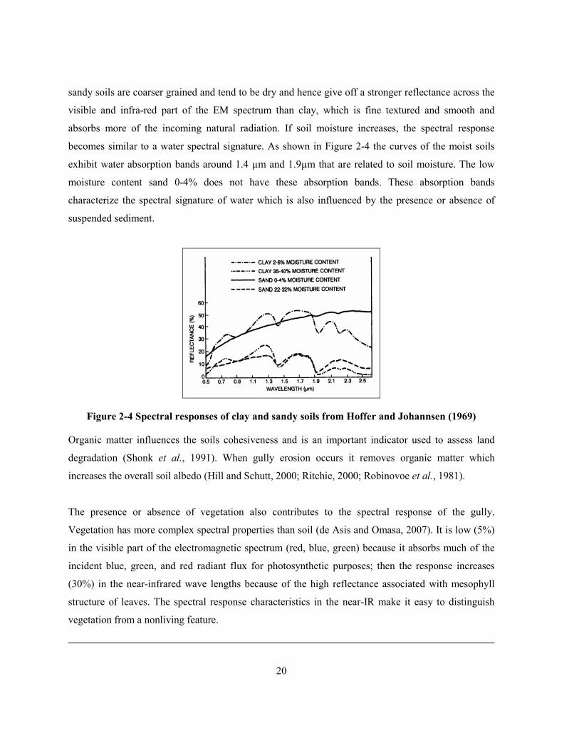
Figure 2-4 is a graph showing the differences in the spectral signatures of two bare soils; clay and
sand (solid line and large dashed line). The differences in the spectral curves of the clay (2-6%
moisture content) and the sand (0-4% moisture content) relates to the differences in soil texture;
20
sandy soils are coarser grained and tend to be dry and hence give off a stronger reflectance across the
visible and infra-red part of the EM spectrum than clay, which is fine textured and smooth and
absorbs more of the incoming natural radiation. If soil moisture increases, the spectral response
becomes similar to a water spectral signature. As shown in Figure 2-4 the curves of the moist soils
exhibit water absorption bands around 1.4 µm and 1.9µm that are related to soil moisture. The low
moisture content sand 0-4% does not have these absorption bands. These absorption bands
characterize the spectral signature of water which is also influenced by the presence or absence of
suspended sediment.
Figure 2-4 Spectral responses of clay and sandy soils from Hoffer and Johannsen (1969)
Organic matter influences the soils cohesiveness and is an important indicator used to assess land
degradation (Shonk et al., 1991). When gully erosion occurs it removes organic matter which
increases the overall soil albedo (Hill and Schutt, 2000; Ritchie, 2000; Robinovoe et al., 1981).
The presence or absence of vegetation also contributes to the spectral response of the gully.
Vegetation has more complex spectral properties than soil (de Asis and Omasa, 2007). It is low (5%)
in the visible part of the electromagnetic spectrum (red, blue, green) because it absorbs much of the
incident blue, green, and red radiant flux for photosynthetic purposes; then the response increases
(30%) in the near-infrared wave lengths because of the high reflectance associated with mesophyll
structure of leaves. The spectral response characteristics in the near-IR make it easy to distinguish
vegetation from a nonliving feature.

21
The time and stage dimension of a gully erosion process affects the physical and spectral properties of
the soil surface (Ritchie, 2000). For example Figure 2-5 shows a cross-section of a gully system that
has developed through incision into a thin colluvium layer overlying mudstones and sandstones in
Lugxogxo, South Africa (Dardis, 1991). The spectral response of this gully system would vary. Water
may or may not be present in the base of the gully and each of the layers (colluvium, palaeosol,
mudstone, dolerite, gravel lag) and each of the stages (1,2,3 and 4) shown in the cross-section, would
have different spectral signatures and may also have different types of vegetation growing on them
depending on the mix of these surface types. Usually a stabilized gully has more vegetation present
than an actively eroding gully in which bare soil dominates. During the rainy season the more
stabilized gully would then have more healthy vegetation within the gully meaning that there would
be an increase in the reflectance of the NIR in the spectral signature.
Figure 2-5 An example of soil variability within a gully that has incised into a thin colluvium
layer overlying mudstones and subordinate sandstones. Left are four cross-sections of the gully
system at different points. Right is an aerial view of the gully system with graphs displaying
elevation change in the landscape (A,B,C,and D). Modified from (Dardis, 1991).

22
Since gullies are complex features to map, the design of a remote sensing gully mapping technique
needs to maximize the spectral response of the eroded area (Dwivedi and Ramana, 2003; Metternicht
and Fermont, 1998; Pickup and Nelson, 1984; Pickup and Chewings, 1988) and/or the erosion
controlling factors (Cyr et al., 1995; Hochschild et al., 2003; Price, 1993). The complex nature of the
gullies and of the surrounding terrain, within which they are formed, has brought remote sensing to
the forefront of gully erosion mapping with a stated need for improved gully mapping methods using
satellite remote sensing (Boardman, 2006; Lal, 2001).
2.3.2.2.1 Spectral Behavior of Gullies in a Landsat TM Imagery
The amount of energy reflected from an object, for example gully or an erosion factor, can be graphed
at specific wavelengths to produce a spectral reflectance curve (Jensen, 2005). The spectral
reflectance curves are unique to the sample and the environment from which they are derived
(Schowengerdt, 2007).
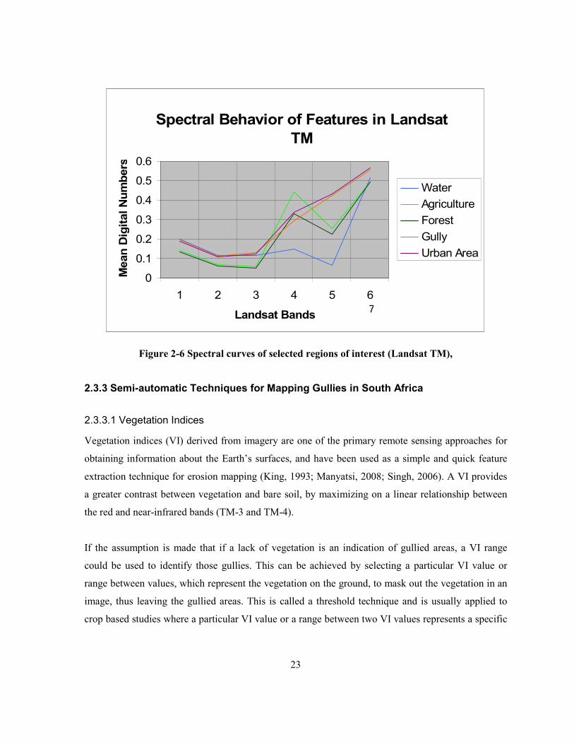
Figure 2-6 displays the spectral response (mean reflectance) of six regions of interests (ROI) in bands
1-5 and band 7 of Landsat TM data of KwaZulu-Natal, South Africa. The lower reflectance of the
gully ROI in the visible and near-infrared ranges compared to the other bands is attributed to a
shadow component related to depth of the gullies and the irregularities of the surface, trapping more
of the incoming sunlight and reducing the amount of reflected energy (Metternicht and Zinck, 1998).
The gully and urban ROI, indicated as a brown and purple solid line respectively, exhibits the highest
reflectance values in all waveband ranges, except the TM-4 where maximum reflectance values
correspond to ROIs consisting of more green vegetation, forest and agriculture. The TM bands 4 and
5 allow for the most separability amongst the ROIs yet in TM bands 1, 2 and 3 the ROIs are less
separable because of the similarity in their interactions with the sun’s rays. This similarity can cause
difficulties when trying to identify gullies spectrally from other features in the landscape; thus most
remote sensing studies have focused on extracting erosion controlling factors such as soils (Pickup
and Nelson, 1984; Pickup and Chewings, 1988) and vegetation (Singh et al., 2004; Wessels et al.,
2004). However, remote sensing techniques do exist that can help enhance separability amongst
classes for example vegetation indices and classification algorithms.
23
Figure 2-6 Spectral curves of selected regions of interest (Landsat TM),
2.3.3 Semi-automatic Techniques for Mapping Gullies in South Africa
2.3.3.1 Vegetation Indices
Vegetation indices (VI) derived from imagery are one of the primary remote sensing approaches for
obtaining information about the Earth’s surfaces, and have been used as a simple and quick feature
extraction technique for erosion mapping (King, 1993; Manyatsi, 2008; Singh, 2006). A VI provides
a greater contrast between vegetation and bare soil, by maximizing on a linear relationship between
the red and near-infrared bands (TM-3 and TM-4).
If the assumption is made that if a lack of vegetation is an indication of gullied areas, a VI range
could be used to identify those gullies. This can be achieved by selecting a particular VI value or
range between values, which represent the vegetation on the ground, to mask out the vegetation in an
image, thus leaving the gullied areas. This is called a threshold technique and is usually applied to
crop based studies where a particular VI value or a range between two VI values represents a specific
Spectral Behavior of Features in Landsat
TM
0
0.1
0.2
0.3
0.4
0.5
0.6
1 2 3 4 5 6
Landsat Bands
Mean
Dig
ital N
um
bers
Water
Agriculture
Forest
Gully
Urban Area
7

24
vegetation/crop type (Vaidyanathan et al., 2002). To apply this technique for mapping gullies in
South Africa, the selected VI must accurately represent the vegetation on the ground.
2.3.3.1.1 Normalized Difference Vegetation Index
Normalized difference vegetation index (NDVI) can easily be derived from data acquired by a variety
of satellites and low value thresholds can be selected to extract eroded areas (Mathieu et al., 1997;
Symeonakis and Drake, 2004; Thiam, 2003; Vaidyanathan et al., 2002). Using SPOT imagery,
Mathieu et al. (1997) mapped gully erosion in northern France by calculating NDVI and doing a
maximum similarity with a brightness index (BI) and masking out vegetation, limestone outcrops and
built-up areas. Thiam (2003) also used NDVI to produce a three-class (low, moderate, and high) land
degradation risk map using multitemporal 1km NOAA/AVHRR. Here NDVI values were averaged
for specific soil types which allowed for the evaluation the spatial extent of land degradation risk in
southern Mauritius. Symeonakis and Drake (2004) used NDVI as an indicator of vegetation cover to
determine areas of desertification over sub-Saharan Africa, using AVHRR. Using imagery from the
Indian satellite sensor IRS-1B LISS-II, Vaidyanathan et al. (2002) used NDVI thresholds to identify
classes for an erosion intensity map in Garhwal. This technique allowed for separation of 4 different
classes, snow (NDVI <-0.01), vegetation (0.03 ≥ NDVI > -0.01), Barren (0.03≥NDVI>0.14), Water
(0.14 ≥ NDVI > 0.34) (Vaidyanathan et al., 2002).
NDVI measures the slope of the line between the point of convergence and the location of the pixel
plotted in red-NIR space (Baugh and Groeneveld, 2006). This index is computed by dividing the
difference of the near-IR and visible red bands (bands 3 and 4) by their sum, as seen in the following
equation:
NDVI = (NIR-R) / (NIR+R) (2-1)
This equation is based on the idea that chlorophyll absorbs incoming radiation in the red/visible band
and that the interior structure of the plant leaves reflects strongly in the near-infrared (indication of
plants health). Although this equation is simple NDVI has proven to be unsuitable for areas with
sparse vegetation. This is because soil is a major surface component that controls the spectral
behavior of sparsely vegetated areas (Huete, 1988).

25
2.3.3.1.2 Soil Line Indices
In attempts to improve the detection of erosion features, in sparsely vegetated areas, other studies
have applied vegetation indices developed to minimize the effect of soil, such as the soil adjusted
vegetation index (SAVI) (Botha and Fouche, 2000) and the transformed soil adjusted vegetation
index (TSAVI) (Hochschild et al., 2003). These indices are designed to be relatively insensitive to
variables such as soil background, sun-sensor angular geometry and the atmosphere (Dash et al.,
2007), which NDVI is sensitive to.
SAVI was originally developed using ground-based data, but it was later found useful in minimizing
soil background effects using satellite imagery (Jackson and Huete, 1991). SAVI has been used in
land degradation studies in southern Africa (Botha and Fouche, 2000). Using Landsat TM and MSS,
Botha (2000) used SAVI to detect land degradation change. Whereas Dang et al. (2003) used Landsat
ETM to calculated SAVI for a soil erosion model for Miyun County in China.
SAVI and TSAVI are based on the assumption that bare soil reflectance lies on a single line in the
feature space of the red and NIR bands (soil line) (Baret et al., 1993). The red and NIR bands have
proven to be very useful for identifying soil erosion through the use of the ‘soil line’ concept
(Mathieu et al., 1997) which is a linear relationship between bare soil reflectance observed in the red
and near-IR bands (Richardson and Wiegand, 1977). This soil line is characterized by the following
linear equation:
NIR = aR+b (2-2)
Where a is the soil line slope and b is the y intercept. In theory the soil line can be calculated by
finding two patches of different soils and calculating the best fitted line in NIR-red spectral space
(Baugh and Groeneveld, 2006). In practice, the typical approach is to collect a large number of pixels
and plot them on a NIR-red spectral space (y-axis NIR, x-axis red), then use the flat edge as the soil
line (Baugh and Groeneveld, 2006). Soil Adjusted Vegetation Index (SAVI) was proposed by Huete
(1988). It is derived from NDVI and can be expressed in terms of the NIR and R reflectance and also
a constant (L), according to the following:
SAVI = [(NIR-R) / (NIR+R+L)] (1+L) (2-3)

26
The value of L ranges from 0, for very high vegetation cover, to 1 for very low vegetation cover.
Huete, (1988) proved that SAVI (L=0.5) successfully minimizes soil variations in both the grass and
the cotton canopies (Huete, 1988). Huete et al. (1992) showed that SAVI normalized the soil
background (dry, wet, and damp soils) across all viewing angles. Some of the drawbacks of SAVI is
it only offers an exact solution for study sites where the soil line slope is exactly in unity and the
intercept is exactly zero (Fox et al., 2004).
Another VI expression used is the TSAVI which can significantly reduce the effects of soil for areas
of sparse vegetation cover or bare soil (Baret and Guyot, 1991; Hochschild et al., 2003). It
incorporates soil line parameters which allow for a VI that is designed for a specific area and can be
applied in imagery that covers different soil types. Low TSAVI values have been related to
potentially degraded areas (Flugel et al., 2003; Hochschild et al., 2003). Calculation of TSAVI
requires parameters that are developed from a soil line. It is important to note that these parameters
vary with soil type.
TSAVI= a(NIR-aRed-b) / (aNIR+Red-ab+X(1+a²)) (2-4)
Where a and b are calculated from the soil line as slope and y intercept respectively, and X is a soil
adjustment factor (Baret and Guyot, 1991). The benefit of using TSAVI is that it adjusts to a given
study area using a well designed soil line; hence it would be expected to perform better than SAVI
and NDVI as they are universal (Lawrence and Ripple, 1998). Though there is little literature on the
application of soil line vegetation indices (SAVI and TSAVI) in erosion research, they could prove to
be beneficial for gully erosion mapping in South Africa.
2.3.3.2 Classification Algorithms
A second approach of applicability to mapping soil erosion using remote sensing is through the use of
the powerful capabilities of supervised classification algorithms. The objective of a supervised
classification approach is to automatically categorize all pixels in an image based on their spectral
clustering behavior, into classes or themes; in the case of this research those classes would be gullies
and non gullies. The classification process involves three main steps (i) Transformation – the
transformation of an image by spatially or spectrally enhancing feature identification, for example
Principal Component Analysis (PCA). This helps remove noise in the image and simplifies the
calculations performed by an algorithm, (ii) Training – selection of pixels which are used to train the
classifier to recognize classes, and determination of decision boundaries which partition the feature

27
space according to the training pixel properties, (iii) Labeling – the application of the feature space
decision boundaries to the entire image to label all pixels (Schowengerdt, 2007). The final output is a
thematic map that categorizes different surface materials or conditions (see Figure 2-7).
Figure 2-7 The classification process (modified from Schowengerdt, 2002)
Classification algorithms can be parametric or non-parametric. Both require user input, in the form of
training data, to guide the image processing software through the classification. A parametric
algorithm uses parameters such as mean and variance-covariance matrices for each of the classes to
determine its decision boundary between classes; whereas non-parametric algorithms do not make
Transformation
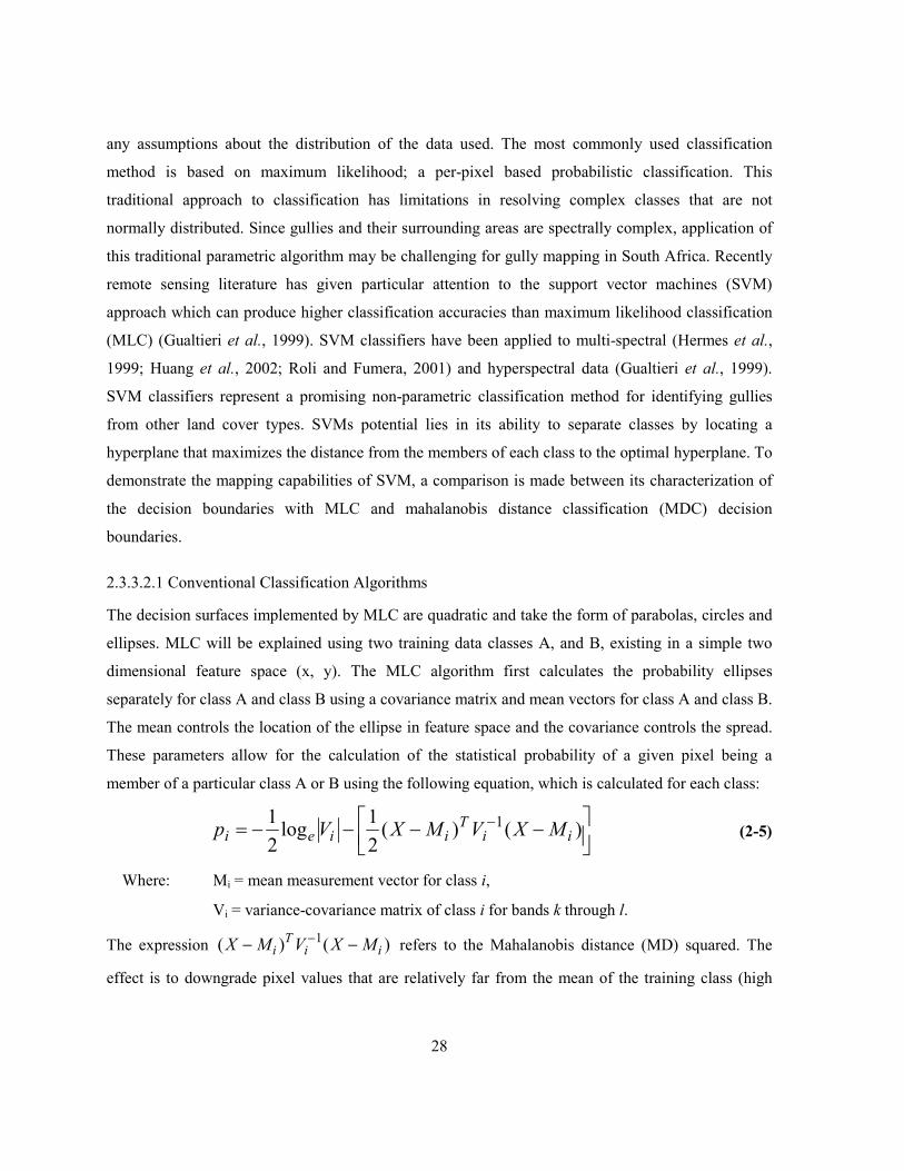
28
any assumptions about the distribution of the data used. The most commonly used classification
method is based on maximum likelihood; a per-pixel based probabilistic classification. This
traditional approach to classification has limitations in resolving complex classes that are not
normally distributed. Since gullies and their surrounding areas are spectrally complex, application of
this traditional parametric algorithm may be challenging for gully mapping in South Africa. Recently
remote sensing literature has given particular attention to the support vector machines (SVM)
approach which can produce higher classification accuracies than maximum likelihood classification
(MLC) (Gualtieri et al., 1999). SVM classifiers have been applied to multi-spectral (Hermes et al.,
1999; Huang et al., 2002; Roli and Fumera, 2001) and hyperspectral data (Gualtieri et al., 1999).
SVM classifiers represent a promising non-parametric classification method for identifying gullies
from other land cover types. SVMs potential lies in its ability to separate classes by locating a
hyperplane that maximizes the distance from the members of each class to the optimal hyperplane. To
demonstrate the mapping capabilities of SVM, a comparison is made between its characterization of
the decision boundaries with MLC and mahalanobis distance classification (MDC) decision
boundaries.
2.3.3.2.1 Conventional Classification Algorithms
The decision surfaces implemented by MLC are quadratic and take the form of parabolas, circles and
ellipses. MLC will be explained using two training data classes A, and B, existing in a simple two
dimensional feature space (x, y). The MLC algorithm first calculates the probability ellipses
separately for class A and class B using a covariance matrix and mean vectors for class A and class B.
The mean controls the location of the ellipse in feature space and the covariance controls the spread.
These parameters allow for the calculation of the statistical probability of a given pixel being a
member of a particular class A or B using the following equation, which is calculated for each class:
−−−−= − )()(2
1log
2
1 1ii
Tiiei MXVMXVp (2-5)
Where: Mi = mean measurement vector for class i,
Vi = variance-covariance matrix of class i for bands k through l.
The expression )()( 1ii
Ti MXVMX −− −
refers to the Mahalanobis distance (MD) squared. The
effect is to downgrade pixel values that are relatively far from the mean of the training class (high

29
MD) taking into account the shape of the probability distribution of the training-class members
(Mather, 2004). The unknown pixel is assigned to the class that produces the largest probability.
The above discussion on how an unknown pixel (w) is classified, is illustrated in Figure 2-8, which is
two classes A and B in a two dimensional feature space (x,y). Here class A has a high positive
covariance between the bands x and y whereas class B has a lower covariance, this is demonstrated in
the width of the ellipses. The means of each class are located in the centre of the ellipse, point 1 and
2. The contours indicate the degree of probability of point w belonging to each class, so as one moves
away from the mean or centroid, the probability of the pixel w being in that class decreases. The
shape of the probability distribution contours also controls the probability of whether or not a pixel
should belong in that class as can be seen point w is closer the center of class A yet because of the
shape of the ellipse point w is more likely to be classified as class B rather than class A. Probability
thresholds can also be applied if not enough training data are available to estimate the parameters of
the class distributions. Applying a threshold
also helps remove outliers. Thus the MLC can
be regarded as a distance-like classifier
because it measures the distance from the
unknown pixel to each class however this is
modified according to class (Mather, 2004).
There exists abundant literature on ML and its
application to remote sensing data; for more
information a comprehensive overview can be
found in (Jensen, 2005; Richards and Jia,
2006).
Figure 2-8 Displays class A and class B plotted in an x-y feature space, with hypothetical
probability contours and means. Modified from Mather (2004)
The Mahalanobis distance classifier (MDC) is similar to MLC however its decision boundaries
assume all class covariance’s are equal (Richards and Jia, 2006) and simply measures the MD of an
unknown pixel as appose to MLC which calculates the probability density function of each class.
Here the MD is defined as the distance of an unknown pixel from the center of a class ellipse (i.e.
mean) divided by the width of the ellipsoid in the direction of the unknown pixel (Mather, 2004). An
Class A
Class B
w1
2
x
y
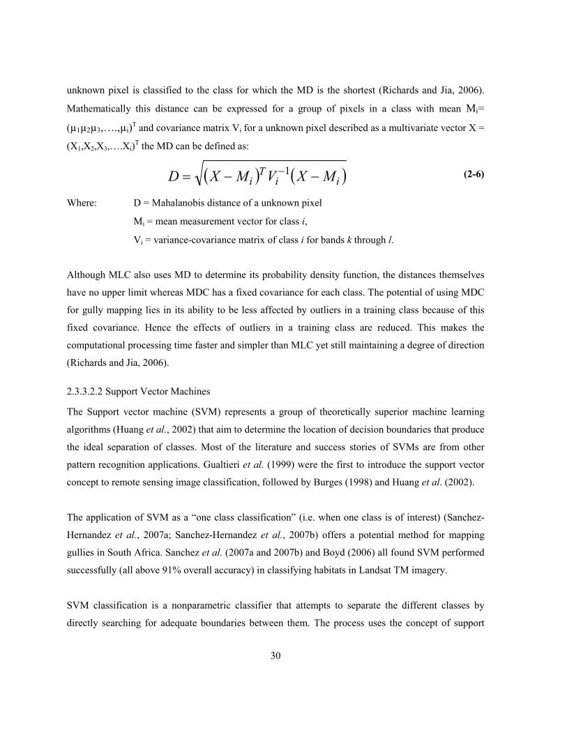
30
unknown pixel is classified to the class for which the MD is the shortest (Richards and Jia, 2006).
Mathematically this distance can be expressed for a group of pixels in a class with mean Mi=
(µ1µ2µ3,….,µi)T and covariance matrix Vi for a unknown pixel described as a multivariate vector X =
(X1,X2,X3,….Xi)T the MD can be defined as:
( ) ( )iiT
i MXVMXD −−= −1
(2-6)
Where: D = Mahalanobis distance of a unknown pixel
Mi = mean measurement vector for class i,
Vi = variance-covariance matrix of class i for bands k through l.
Although MLC also uses MD to determine its probability density function, the distances themselves
have no upper limit whereas MDC has a fixed covariance for each class. The potential of using MDC
for gully mapping lies in its ability to be less affected by outliers in a training class because of this
fixed covariance. Hence the effects of outliers in a training class are reduced. This makes the
computational processing time faster and simpler than MLC yet still maintaining a degree of direction
(Richards and Jia, 2006).
2.3.3.2.2 Support Vector Machines
The Support vector machine (SVM) represents a group of theoretically superior machine learning
algorithms (Huang et al., 2002) that aim to determine the location of decision boundaries that produce
the ideal separation of classes. Most of the literature and success stories of SVMs are from other
pattern recognition applications. Gualtieri et al. (1999) were the first to introduce the support vector
concept to remote sensing image classification, followed by Burges (1998) and Huang et al. (2002).
The application of SVM as a “one class classification” (i.e. when one class is of interest) (Sanchez-
Hernandez et al., 2007a; Sanchez-Hernandez et al., 2007b) offers a potential method for mapping
gullies in South Africa. Sanchez et al. (2007a and 2007b) and Boyd (2006) all found SVM performed
successfully (all above 91% overall accuracy) in classifying habitats in Landsat TM imagery.
SVM classification is a nonparametric classifier that attempts to separate the different classes by
directly searching for adequate boundaries between them. The process uses the concept of support
31
vectors8 to identify the optimal separating hyperplane OHS (multidimensional linear surface) which
divides two classes and functions as a decision surface for classification. The orientation of the
hyperplane is where there is a maximum separation between the two classes which is essentially
called maximizing the margin. If two-classes are linearly separable the SVM selects from among the
infinite number of linear decision boundary the one that has low generalization error (Gualtieri et al.,
1999).
However most classes are not linearly separable and in such cases the SVM approach uses a kernel
which plays an important role in locating complex decision boundaries between classes (Huang et al.,
2002). The kernel maps the data to a higher dimensional space and within that space it attempts to
find a linear separating surface between the two classes (Gualtieri et al., 1999). The basic idea is the
nonlinearly separable data appear in the training algorithm are in the form of dot products (xi*xj) and
the kernel maps them to some other Euclidean space where they can be linearly separated. (See
Figure 2-9).
8 Training samples that lie near the boundary between the classes in feature space (Boyd, Sanchez-Hernandez,
and Foody, 2006)

32
a) Input Space b) Feature space
The kernel maps the training samples into a higher dimensional
Kernel Mapping
function
Optimal H
yper
plane
Legend
Class 1
Class 2
Figure 2-9 The kernel maps the training samples into a higher dimensional feature space via a
nonlinear function and constructs a separating hyperplane with maximum margins. Modified
from Camps-Valls et al. (2004)
How the kernel operates is by introducing positive slack variables (allowed errors) and a penalization
parameter C which is applied to the errors (Camps-Valls et al., 2004). The positive slack variables are
applied to each sample and indicate the distance the sample is from the OSH. They are used so that
the amounts of violation of the constraints are introduced. The constant C is selected by the user and
is used to control the magnitude of the penalty that is associated with the samples that lie on the
wrong side of the decision boundary (Foody et al., 2006). Parameter C affects the generalization
capabilities of the classifier (Camps-Valls et al., 2004). Large values of C may cause the SVM to
over-fit the training data and low values may cause an inappropriately large fraction of support
vectors to be derived (Foody et al., 2006). Figure 2-10 is a more detailed description of how the SVM
operates with linear and nonlinear training data. This binary classification can also be extended to N
classes, where N > 2 (Hsu and Lin, 2002), however this is not the focus of the study. For more
information the kernel functions and parameters please refer to Vapkin (1995).
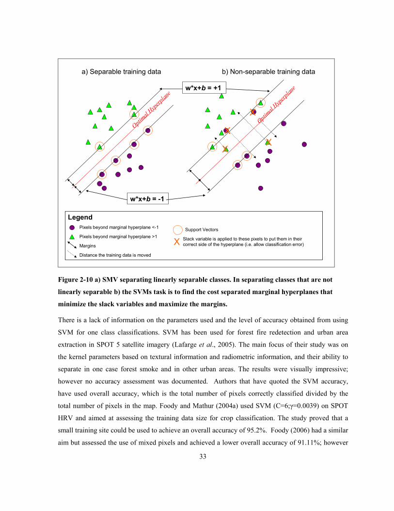
33
w*x+b = +1
w*x+b = -1
Opt
imal
Hyp
erpl
ane
Opt
imal H
yper
plan
e
a) Separable training data b) Non-separable training data
X
X
X
X
Legend
X
Support Vectors
Slack variable is applied to these pixels to put them in their
correct side of the hyperplane (i.e. allow classification error)
Pixels beyond marginal hyperplane <-1
Pixels beyond marginal hyperplane >1
Margins
Distance the training data is moved
Figure 2-10 a) SMV separating linearly separable classes. In separating classes that are not
linearly separable b) the SVMs task is to find the cost separated marginal hyperplanes that
minimize the slack variables and maximize the margins.
There is a lack of information on the parameters used and the level of accuracy obtained from using
SVM for one class classifications. SVM has been used for forest fire redetection and urban area
extraction in SPOT 5 satellite imagery (Lafarge et al., 2005). The main focus of their study was on
the kernel parameters based on textural information and radiometric information, and their ability to
separate in one case forest smoke and in other urban areas. The results were visually impressive;
however no accuracy assessment was documented. Authors that have quoted the SVM accuracy,
have used overall accuracy, which is the total number of pixels correctly classified divided by the
total number of pixels in the map. Foody and Mathur (2004a) used SVM (C=6;γ=0.0039) on SPOT
HRV and aimed at assessing the training data size for crop classification. The study proved that a
small training site could be used to achieve an overall accuracy of 95.2%. Foody (2006) had a similar
aim but assessed the use of mixed pixels and achieved a lower overall accuracy of 91.11%; however

34
still concluded that SVM was comparable to conventional methods (91.48% overall accuracy). More
recently Mathur and Foody (2008) used SVM (C=1; γ=0.000625) to classify crops in South west
India. They demonstrated that using only the support vectors, for the SVM classification, still
produced a high overall accuracy of 90% which is comparable to the conventional training data which
had a 92% overall accuracy.
Rational for using Support Vector Machines for gully mapping in South Africa
• It has proven successful in binary classifications (Boyd et al., 2006; Sanchez-Hernandez et
al., 2007b; Tax and Duin, 2004) which separate the class of interest from all other classes. In
this case gullies from non gully areas.
• Is well adapted to deal with data of high dimensions: Since SVM does not rely explicitly
on the dimensionality of the training data but uses pattern recognition, regression, and density
estimation in high-dimensional spaces to separate the classes (Vapnik, 1998), this means that
less time is required in creating training data.
• Less expert knowledge is required in training data collection: The nature of SVM’s
operation allows the use of smaller training data size (Foody and Mathur, 2004b). SVM has
also proven useful for mapping unknown classes in a Landsat ETM (Mantero and Moser,
2005). Therefore, SVM implementation is probably more tolerable of less expert knowledge
when identifying training data for mapping gullies using this algorithm.
• Competitive with other classifiers: It has been proven to be competitive with the best
available classification methods such as neural networks and decision tree classifiers (Huang
et al., 2002); and typically yields accuracies that are comparable to other classifiers that are
widely used in remote sensing (Foody and Mathur, 2004a; Huang et al., 2002). Other
classifiers have problems separating unbalanced classes.
If SVM is successful in gully mapping then researchers will be able to extract gully information with
little background knowledge of the gully feature/process, rapidly and inexpensively, over large
geographic area (50-10,000km²). Fortunately most of the remote sensing literature on SVM
classification has provided information on the level of accuracy; however, in most of these studies
these values are very misleading and could, once again, contribute to some serious issues when
drawing conclusions on maps created using classification algorithms.
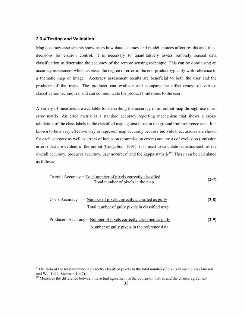
35
2.3.4 Testing and Validation
Map accuracy assessments show users how data accuracy and model choices affect results and, thus,
decisions for erosion control. It is necessary to quantitatively assess remotely sensed data
classification to determine the accuracy of the remote sensing technique. This can be done using an
accuracy assessment which assesses the degree of error in the end-product typically with reference to
a thematic map or image. Accuracy assessment results are beneficial to both the user and the
producer of the maps. The producer can evaluate and compare the effectiveness of various
classification techniques, and can communicate the product limitations to the user.
A variety of measures are available for describing the accuracy of an output map through use of an
error matrix. An error matrix is a standard accuracy reporting mechanism that shows a cross-
tabulation of the class labels in the classified map against those in the ground truth reference data. It is
known to be a very effective way to represent map accuracy because individual accuracies are shown
for each category as well as errors of inclusion (commission errors) and errors of exclusion (omission
errors) that are evident in the output (Congalton, 1991). It is used to calculate statistics such as the
overall accuracy, producer accuracy, user accuracy9 and the kappa statistic
10. These can be calculated
as follows:
Overall Accuracy = Total number of pixels correctly classified
Total number of pixels in the map
(2-7)
Users Accuracy = Number of pixels correctly classified as gully
Total number of gully pixels in classified map
(2-8)
Producers Accuracy = Number of pixels correctly classified as gully
Number of gully pixels in the reference data
(2-9)
9 The ratio of the total number of correctly classified pixels to the total number of pixels in each class (Janssen
and Wel 1994, Stehman 1997), 10
Measures the difference between the actual agreement in the confusion matrix and the chance agreement

36
Kappa Statistic =
∑
∑ ∑
=++
= =++
−
−
k
i
ii
k
i
k
i
iiii
nnn
nnnn
1
2
1 1
(2-10)
Where: n the total number of samples
nii the number of samples correctly classified into category i
ni+ the number of samples classified into category i in the classified image
n+I is the number of samples classified into category j in the reference data set
There are many claims on which measurement is the best for quoting the accuracy of a given
classification. Interestingly enough, most of the remote sensing erosion studies have failed to report
the accuracy of the output maps (Vrieling, 2006) and those that have provided validation statistics, are
often misleading. For example, Ellis (2000) study on classification of soil erosion in Australia used
overall accuracy to compare two classifiers performances. However the high overall accuracies
reported was mostly a result of two classes which occupied 99% of the study region: `no appreciable
erosion' (class 1) and `minor sheet erosion (Ellis, 2000). Other classifications where one class is of
interest, have quoted the maps based on either the producer or the user accuracy. For example, both
Boyd et al. (2006) and Sanchez-Hernandez (2007a) chose the producer accuracy as being more
important for identifying habitats for fen identification; whereas, Verling (2007) placed more
emphasis on the user accuracy for identifying gullies. Verling (2007) also suggested that using an
average of the producer and user accuracy for identifying gullies is less biased than reporting a single
value. It is not clear, however, whether such a technique could be used for a comparative study of
different classifications. Stehman (1997) favored the kappa statistics for comparison of classified
maps using different algorithms.
To illustrate how some of the above accuracy measurements could be very misleading for a
comparison of classified maps representing gullies and non gullies in this study, we consider the
calculations presented in Figure 2-11. This is a hypothetical example displaying two maps; classified
map and reference map each showing different proportions of area for the gully and no gullied class.
The accuracy assessment is illustrated in the bottom left and shows correctly classified pixels as solid
colour and errors of commission and omission as patterned areas. The error matrix in the top right
now displays the values which are used in the calculation of the accuracy measurements.
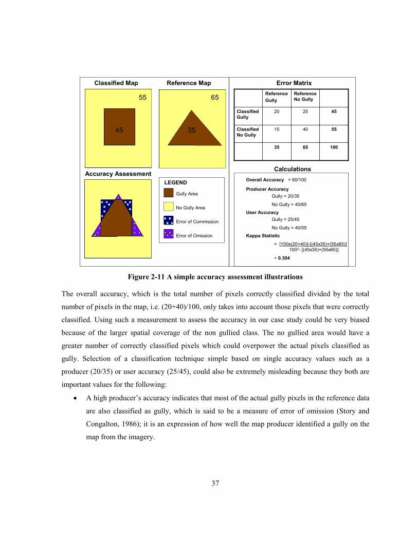
37
1006535
554015Classified
No Gully
452520Classified
Gully
Reference
No Gully
Reference
Gully
45 35
6555
Classified Map Reference Map
Accuracy Assessment
Gully Area
No Gully Area
Error of Commission
Error of Omission
LEGEND
Gully = 20/35
No Gully = 40/65
Calculations
User Accuracy
Producer Accuracy
Overall Accuracy = 60/100
Gully = 25/45
No Gully = 40/55
Kappa Statistic
= [100x(20+40)]-[(45x35)+(55x65)]
100²- [(45x35)+(55x65)]
= 0.304
Error Matrix
Figure 2-11 A simple accuracy assessment illustrations
The overall accuracy, which is the total number of pixels correctly classified divided by the total
number of pixels in the map, i.e. (20+40)/100, only takes into account those pixels that were correctly
classified. Using such a measurement to assess the accuracy in our case study could be very biased
because of the larger spatial coverage of the non gullied class. The no gullied area would have a
greater number of correctly classified pixels which could overpower the actual pixels classified as
gully. Selection of a classification technique simple based on single accuracy values such as a
producer (20/35) or user accuracy (25/45), could also be extremely misleading because they both are
important values for the following:
• A high producer’s accuracy indicates that most of the actual gully pixels in the reference data
are also classified as gully, which is said to be a measure of error of omission (Story and
Congalton, 1986); it is an expression of how well the map producer identified a gully on the
map from the imagery.

38
• A high user’s accuracy indicates that few actual non gully pixels are classified as gully,
which is considered a measure of commission (Story and Congalton, 1986). It expresses how
well a user will find that gully feature on the ground.
Since both the user and the producer accuracy are important, the Kappa statistic is more applicable for
assessing the accuracy of a classification output because it takes into account the overall statistical
agreement of an error matrix (Lu and Weng, 2007). The kappa statistic measures the difference
between the actual agreement and the chance agreement and takes into account the whole error matrix
(Congalton, 1991). The value of the kappa statistic ranges from 0 to 1 with values greater than 0.80
indicating a positive correlation between the classified image and the reference data and values
between 0.4 and 0.8 representing a moderate level of agreement (Jensen, 2005). A major advantage of
using the kappa statistic is it allows for a statistical test of the significance of difference between two
techniques (Congalton, 1991) which allows for better comparison.
2.4 Specific Objectives
From this literature review, the main aim of this study is to assess the relative merits of using
vegetation indices and classification algorithms for mapping gullies in a Landsat TM imagery of KZN
South Africa. Gullies mapped in a SPOT 5 Pan image using traditional digitization provide a
comparative basis for this assessment. The specific objectives are to compare and evaluate the
classification map accuracy, achieved form each technique with changes in scale of the study area
from the gully system level- continuous and discontinuous to the sub-catchment. The kappa statistic is
the main accuracy assessment metric used. These main objectives can be summarized as follows:
A. Vegetation Indices for mapping gullies:
• To determine the input parameters for TSAVI.
• To determine the best threshold range for gully mapping using NDVI, SAVI and TSAVI.
• To determine the accuracy assessment of the sub-catchment subset using thresholds obtained
from the continuous gully subset.
• To determine the classification accuracy, using the kappa statistic, of the gully maps
produced from NDVI, SAVI and TSAVI in the continuous and discontinuous and sub-
catchment subsets.

39
B. Classification algorithms for mapping gullies:
• To test the need for image transformation for MLC, MDC and SVM for mapping gullies.
• To test the effect in classification accuracy with different training data sizes
• To determine the SVM parameters for gully mapping using Landsat TM.
• To determine the classification accuracy, using the kappa statistic, of the gully maps
produced from MLC, MDC, and SVM in the continuous and discontinuous and sub-
catchment subsets.
The experiments reported in this thesis were undertaken in order to achieve the objectives listed
above, while at the same time addressing a variety of other issues that are extremely important for
successful applications of remote sensing for gully mapping in South Africa such as cost, time and
expert knowledge required.
The final question is whether “medium resolution multi-spectral satellite observations, such as
Landsat TM, combined with information extraction techniques, such as Vegetation Indices and
multispectral classification algorithms, can provide a semi-automatic method of mapping gullies and
to what level of accuracy?”. By addressing this question, it may be possible to determine whether or
not such techniques could improve the ability of developing countries, such as South Africa, to create
gully maps for a large area on ‘the fly’, economically and with little expert knowledge.
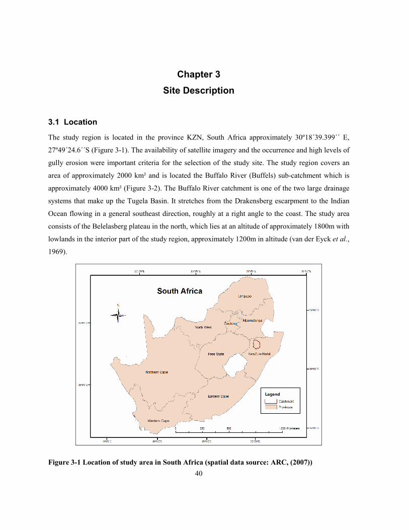
40
Chapter 3
Site Description
3.1 Location
The study region is located in the province KZN, South Africa approximately 30º18´39.399´´ E,
27º49´24.6´´S (Figure 3-1). The availability of satellite imagery and the occurrence and high levels of
gully erosion were important criteria for the selection of the study site. The study region covers an
area of approximately 2000 km² and is located the Buffalo River (Buffels) sub-catchment which is
approximately 4000 km² (Figure 3-2). The Buffalo River catchment is one of the two large drainage
systems that make up the Tugela Basin. It stretches from the Drakensberg escarpment to the Indian
Ocean flowing in a general southeast direction, roughly at a right angle to the coast. The study area
consists of the Belelasberg plateau in the north, which lies at an altitude of approximately 1800m with
lowlands in the interior part of the study region, approximately 1200m in altitude (van der Eyck et al.,
1969).
Figure 3-1 Location of study area in South Africa (spatial data source: ARC, (2007))

41
Figure 3-2 Location of study region within Buffalo River sub-catchment (spatial data source:
rivers (DWAF, 2007) towns and catchment (ARC, 2007))
3.2 Climate
The climate of the study area is semi-arid with dry winters and rainy summers. The area generally
experiences a mean annual rainfall between 800-1000mm with most of the precipitation falling
between the summer months of October to March (Schulze et al., 1997). In the upper catchment in
the north of the study area, mean annual rainfall ranges from 780—1,300mm; whereas the interior
part of the study area has a lower mean annual rainfall ranging from 750-980mm. The monthly
minimum and maximum daily temperatures are approximately 11 ºC and 25ºC, respectively; however
temperatures can reach as high as 39ºC in the summer months (October-March). The two main
ecological regions present in the study area are the Highlands in the north and the Interior Basin
which covers most of the study region.

42
3.3 Vegetation
The study region is located within two Biomes: Grassland biome and Savanna biome (Munica and
Rutherford 2006). Within these biomes a total of three bioregions are present: Mesic Highveld
Grassland, Sub Escarpment Grassland and the Sub-escarpment Savanna. These three bioregions
represent a total of eleven different vegetation units which are characterized based on geology, soils,
topography and precipitation (see Appendix B: Bioregion and vegetation unit map) The vegetation
unit description is provided in Appendix C and additional information can be found in Munica and
Rutherford (2006).
The most dominant vegetation unit is the Income Sandy Grassland (approximately 80% of the study
area) which has the greatest erosion intensity compared to the other vegetation units in the study
region (Mucina and Rutherford, 2006). The two vegetation units of the Mesic Highveld Grassland
bioregion are located on the escarpment in the northern part of the study region. The sub-escarpment
Savanna Bioregion covers a very small area found in the south east of the study region. The other
vegetation types are dispersed through out the study region with the Eastern Temperate Freshwater
wetlands occurring close to the rivers and the Northern Afrotemperate Forest occurring on the high
levels of the escarpment.
3.4 Geology and Soils
The study region is underlain by rocks of the Karoo Supergroup which is a sedimentary rock that
formed from the filling of the Karoo basin during the Permo-Carboniferous to Early Jurassic times
(van der Eyck et al., 1969). The sedimentary formation includes four layers: Dwyka, Ecca, Beaufort
and Stormberg series. The majority of the study area (approximately 85%) consists of the Vryheid
and Volkrust formations of the Ecca series and the Normandien formation of the Beaufort series. The
Vryheid formation consists of thick beds of whitish to yellowish, mostly coarse-grained sandstones
and massive grits, often rich in feldspars (Catuneanu et al., 2005). The Volkrust formation consists of
blue shales that were deposited under lacustrine conditions (van der Eyck et al., 1969) (see Figure
3.3). The Normandien formation consists of coarse grained sandstone interbedded with mudstone that
has been deposited by meandering streams (Catuneanu et al., 2005). Scattered within the study area
are intrusive dykes and sills made of a volcanic rock called Karoo Dolerite, as well as alluvial and
colluvial deposits made up of silt, clay and larger particles of sand.
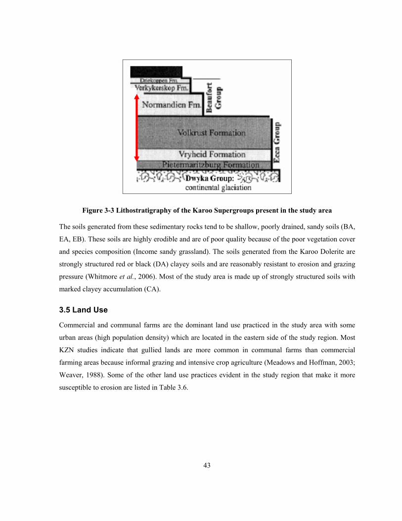
43
Figure 3-3 Lithostratigraphy of the Karoo Supergroups present in the study area
The soils generated from these sedimentary rocks tend to be shallow, poorly drained, sandy soils (BA,
EA, EB). These soils are highly erodible and are of poor quality because of the poor vegetation cover
and species composition (Income sandy grassland). The soils generated from the Karoo Dolerite are
strongly structured red or black (DA) clayey soils and are reasonably resistant to erosion and grazing
pressure (Whitmore et al., 2006). Most of the study area is made up of strongly structured soils with
marked clayey accumulation (CA).
3.5 Land Use
Commercial and communal farms are the dominant land use practiced in the study area with some
urban areas (high population density) which are located in the eastern side of the study region. Most
KZN studies indicate that gullied lands are more common in communal farms than commercial
farming areas because informal grazing and intensive crop agriculture (Meadows and Hoffman, 2003;
Weaver, 1988). Some of the other land use practices evident in the study region that make it more
susceptible to erosion are listed in Table 3.6.
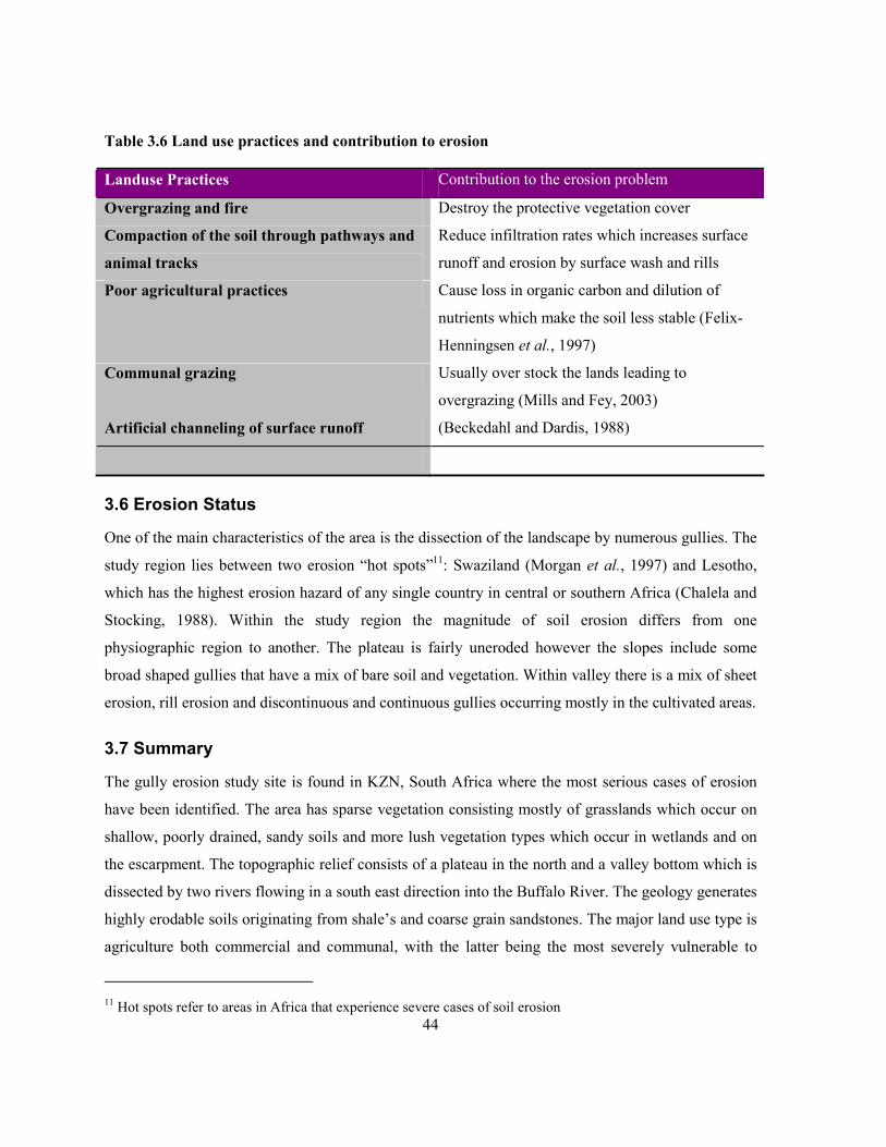
44
Table 3.6 Land use practices and contribution to erosion
Landuse Practices Contribution to the erosion problem
Overgrazing and fire Destroy the protective vegetation cover
Compaction of the soil through pathways and
animal tracks
Reduce infiltration rates which increases surface
runoff and erosion by surface wash and rills
Poor agricultural practices Cause loss in organic carbon and dilution of
nutrients which make the soil less stable (Felix-
Henningsen et al., 1997)
Communal grazing Usually over stock the lands leading to
overgrazing (Mills and Fey, 2003)
Artificial channeling of surface runoff (Beckedahl and Dardis, 1988)
3.6 Erosion Status
One of the main characteristics of the area is the dissection of the landscape by numerous gullies. The
study region lies between two erosion “hot spots”11
: Swaziland (Morgan et al., 1997) and Lesotho,
which has the highest erosion hazard of any single country in central or southern Africa (Chalela and
Stocking, 1988). Within the study region the magnitude of soil erosion differs from one
physiographic region to another. The plateau is fairly uneroded however the slopes include some
broad shaped gullies that have a mix of bare soil and vegetation. Within valley there is a mix of sheet
erosion, rill erosion and discontinuous and continuous gullies occurring mostly in the cultivated areas.
3.7 Summary
The gully erosion study site is found in KZN, South Africa where the most serious cases of erosion
have been identified. The area has sparse vegetation consisting mostly of grasslands which occur on
shallow, poorly drained, sandy soils and more lush vegetation types which occur in wetlands and on
the escarpment. The topographic relief consists of a plateau in the north and a valley bottom which is
dissected by two rivers flowing in a south east direction into the Buffalo River. The geology generates
highly erodable soils originating from shale’s and coarse grain sandstones. The major land use type is
agriculture both commercial and communal, with the latter being the most severely vulnerable to
11 Hot spots refer to areas in Africa that experience severe cases of soil erosion

45
gully erosion. The combination of high rainfalls, sparse vegetation cover, highly erodable soils and
poor land management, are all contributing factors to the gully erosion problem in the area.

46
Chapter 4
Methodology
The imagery used in this thesis was made available by the ARC of South Africa and included
Landsat (TM) 2005, SPOT (HRG) 2006 and SPOT (Pan) 2006 images for the defined study area
(refer to Table 2-1 for imagery characteristics). Only Landsat TM was used for the VI gully mapping
methods and both Landsat (TM) and SPOT (HRG) were used for the classification gully mapping
methods. The SPOT (Pan) was used to create the ground truth map for the accuracy assessment of the
semi-automatically produced gully maps. Figure 4-1 summarizes the procedures used to assess the
explored semi-automatic methods for gully mapping.
Preprocessing
• Calibration
• Geometric correction
• Image subsetting
Major
Gully
SPOT 5
SPOT 5Pan
Classification
• MLC
• MDC
• SVM
Vegetation Index
• NDVI
• SAVI
• TSAVI
Accuracy Assessment
Kappa Statistics
Preprocessing
Semi-automatic Methods
Results
Expert
knowledge
1.Ground Truth Gully Map
1.1
Traditional Method
Subsets
Continuous
Gully
Discontinuous
Gully
Ground truth map
• Gully digitization
• Field work
• Map Validation
Sub-catchment
Subsets
LandsatTM
Figure 4-1 Methodology flow diagram
4.1 Preprocessing
Image preprocessing is necessary before information is extracted from the image because it ensures
that the image is as close to the true radiant energy and spatial characteristics at the time of data

47
collection. The preprocesses carried out in this study were radiometric calibration, atmospheric
correction, geometric correction and Image subsetting
4.1.1 Calibration
A typical radiometric calibration involves several different steps. First the sensor’s digital numbers
(DN) need to be converted to at-sensor radiances (sensor calibration). Second, the at-sensor radiance
values need to be transformed to radiances at the earth’s surface and this stage involves incorporation
of the atmospheric condition at the time of image capture (atmospheric correction). The last stage of
calibration is done by correction for slope and aspect, atmospheric path length variation due to
topographic relief, solar spectral irradiance, solar path atmospheric transmittance, and down-scattered
skylight radiance (Schowengerdt, 2007). Not all of the procedures were necessary for this particular
study area because the terrain is not complex (Song et al., 2001).
4.1.1.1.1 Sensor Calibration
The sensor calibration procedure involves converting the DN values to radiances using calibration
coefficients called “gain” and “offset”. The output is units of radiance-per-DN. It is often assumed
that the gain and offset are constant throughout the sensor’s life; hence the Landsat TM image was
processed to reflectance using a Landsat TM model in ERDAS. This procedure reduced between
scene variability by accounting for sensor gains, offsets, solar irradiance, and solar zenith angle
(Schowengerdt, 2007). It also removed the thermal band 6 in Landsat TM, which was not necessary
for this study. SPOT 5 was kept at DN values because only a small subset of the image was used for
this study; thus between-scene variability would be minor.
4.1.1.1.2 Atmospheric Correction
Atmospheric correction is the removal of effects of the passage of radiation through the atmosphere.
The amount of atmospheric correction depends upon the wavelength of the bands and the atmospheric
conditions (Sabins, 1996). For both Landsat TM and SPOT, scattering is the dominant atmospheric
effect (Song et al., 2001) with band 1 of each image having the highest component of scattered light
and band 7 of Landsat TM having the least.
The Dark Pixel Subtraction technique was used to remove the additive effect of scattered light
because it is one of the oldest, simplest and most widely used procedures for adjusting digital remote
sensing data for effects of atmospheric scattering (Song et al., 2001). However, it is recognized that
48
this is not a complete atmospheric correction. Dark pixel subtraction assumes that the dark object,
water in the case of this study domain, has uniformly zero radiance for all bands, and that any non-
zero measured radiance must be due to the atmospheric scattering into the objects pixels (Song et al.,
2001). In ENVI 4.3 the dark pixel reflectance values were subtracted from every pixel in the
corresponding band for both TM and SPOT.
4.1.2 Geometric Correction
The scanning of remote sensing images introduces a number of geometric distortions that are
classified as systematic and nonsystematic distortions (Sabins, 1996). Nonsystematic distortions are
caused by variations in the spacecraft such as attitude, velocity, and altitude. Systematic distortions
are distortions whose effects are constant and are corrected before the data are distributed. To remove
the nonsystematic distortions a geometric correction was performed by conducting an image to map
registration of the Landsat TM and SPOT 5 images to the national georeferenced Topographic Map of
South Africa. A minimum of 20 ground control points were collected and the average root mean
square (RMS) error of 0.85 pixels was achieved. Ideally one would want an RMS error less than 1
and as close to 0 as possible. These steps were necessary to ensure that any additional spatial data
would overlap exactly.
4.1.3 Image Subsetting
Image subsetting reduces the processing time and allows for behavior trends within techniques. Three
different subsets were obtained: a sub-cathment area of 2000km², and two sample areas, each
approximately 150km² that were characteristic of the study region. One sample included a continuous
gully system and the other included discontinuous gullies (Figure 4-2). The large sub-catchment
subset was selected based on the area of overlapped by two Landsat scenes, a 1991 and 2005 (Figure,
4.2). This allowed for change detection studies in the area using the techniques presented. The smaller
continuous gully subset (150 km² window) consisted of a large representative connected gully system.
The smaller discontinuous gully subset (150 km² window) was chosen in an area that had
representative discontinuous gullies (small not connected eroded areas). Both Landsat TM and SPOT
5 Pan were spatially clipped to the three subset areas. Figure 4-2 displays the sub-catchment subset
location within the Buffalo River sub-catchment area (left) and the locations of the continuous (A)
and discontinuous (B) gully subsets, within a preprocessed true colour Landsat TM image that was
clipped to the sub-catchment subset.

49
Figure 4-2 Left: Map illustrating the sub-catchment level of the study area and the Landsat TM
track/row. Right: The locations of the chosen subsets within the selected preprocessed Landsat
TM sub-catchment subset. Label ‘A’ is the continuous gully system, and label ‘B’ is the
discontinuous gullies
50
4.2 Mapping Methodology
The objective of this study was to compare semi-automatically created gully maps with maps created
using traditional gully mapping methods. Thus a gully map created traditionally is assumed to be a
‘ground truth’ map i.e. everything in the map is assumed to be true. Ground truth based comparison is
a form of accuracy assessment where the whole image is used in the accuracy assessment rather than
randomly selected pixels (see, section 2.3.4). Ground truth accuracy assessment was chosen over a
ground truth point approach because it: avoided issues in choosing the sampling design used to select
reference data; it reflected the ‘true’ class proportions for gully and no-gullied areas; and the approach
enabled identification of misclassified pixels (Congalton, 1991).
4.2.1 Traditional Methods
The specific objectives:
• To determine the location of gullies in the catchment using expert knowledge
• To create a gully erosion map that could be used as a “ground truth” basis for assessing the
semi-automatically created gully erosion maps.
A commonly accepted practice for assessing products derived from coarse resolution data is the use
of a higher resolution satellite data as a reference (Cihlar et al., 2003). Ground truth maps were
created using the traditional gully mapping methods mentioned in section 2.3.4, in the SPOT 5
panchromatic image sub-catchment subset. The procedures used to create the assumed “ground truth”
gully map are summarized in Figure 4.3.

51
Gully Digitization • Expert knowledge of gullies location
• Gullies digitized in ArcMap based on: size,
shape, shadow, tone and colour (reflectance)
texture, pattern and feature association.
“Ground Truth” Gully Map
Map used for Semi - automatic
accuracy assessment
Major
Gully
Field Validation• Erosion assessment
• Ground control points
• Photographs
Update Map
Convert Vector file
Raster
Major
GullySubsets
Continuous
Gully
Discontinuous Gully
Sub-catchment
Map Subsets
SPOT 5 Pan
High spatial
resolution
Imagery of 2.5m
Figure 4-3 Flow diagram of the "Ground Truth" gully maps
Creating the ground truth map involved manually digitizing individual gullies in the SPOT 5 Pan sub-
catchment subset using ArcMap. This was carried out by gully mapping experts at the ARC. Ground
truthing was necessary to validate the digitized gully map and involved confirming that the locations
of the gullies mapped were actually present on the ground. This was conducted during a one week
field study that involved: i) documenting the erosion status (sheet, rill, gully), vegetation cover (%),
land use type, (ii) visual assessment of the erosion extent which was limited to visibility from the road
because most gully areas were on private property, (iii) collection of photographs, and (iv) collection
of ground control points (GCP) using a global positioning system (GPS). Previously collected soil
sample data, in the form of a shape file (point), offered additional information on the erosion
assessment. The GCPs and erosion assessment information were imported into ArcMap and overlaid
with the digitized gully map. Erosion experts corrected the errors of omission or commission by re-
digitizing or deleting features in the gully map. Appendix D displays the location of the expert
mapped gullies, soil samples, and ground truth sites and illustrates the location of a few gully
photographs taken during field research.

52
Once the corrections were made in the ground truth gully map the created vector file was converted to
a binary raster representing two classes: gullies and non gully classes. This is essentially a gully map
which was then subsetted to the selected discontinuous and continuous subsets. Figure 4.5 displays
the gully distribution within the discontinuous (A) and continuous (B) gully subsets. A1 and B1 are
SPOT 5 true colour composites of the area with expert digitized gullies overlaid in red; and A2 and
B2 are the ground truth maps created using traditional mapping methods with the white and black
representing gullies and non gullied areas respectively.
B2
A2A1
B1

53
Figure 4-4 A1 and B1 are the digitized gullies, in red solid line, on a true colour composite of
SPOT 5. A2 and B2 are the gully maps created for the discontinuous and continuous subsets
respectively.
4.2.2 Semi-automatic Methods
The following section discusses the semi-automatic techniques used to create a gully map. Each of
the output maps created were enhanced using a majority analysis. This analysis involved using a 3*3
majority filter where the center pixel in the filter was replaced with the class present in the most of the
surrounding pixels. This process removes spurious pixels that cause noise (‘salt and pepper’ effect)
and in some cases it can increase the accuracy of the map (Jensen, 2005). All semi-automatically
created gully maps assessed based on the ground truth maps created in section 4.2.1 using the
accuracy assessment discussed in section 2.3.4.
4.2.2.1 Mapping Gullies from Vegetation Indices
The specific objectives of this section are:
• To determine the input parameters for TSAVI.
• To determine the best threshold range for gully mapping using NDVI, SAVI and TSAVI.
• To determine the classification accuracy, using the kappa statistic, of the gully maps
produced from NDVI, SAVI and TSAVI in the continuous and discontinuous and sub-
catchment subsets.
4.2.2.1.1 Vegetation Index Implementation
NDVI, SAVI and TSAVI were applied to the continuous and discontinuous subsets defined in section
4.1.2.3. NDVI was calculated by inserting the NIR and Red bands in the NDVI model which was
already built in ENVI 4.3. The SAVI formula (equation 2-3) was translated into a band math equation
(equation 4-1) in ENVI 4.3. Since over 70% of the study area is made up of Income Sandy
Grasslands, SAVI L parameter was chosen to be 0.5 because it is the most ideal value for areas with
such sparse vegetation type (Baret and Guyot, 1991; Huete, 1988; Schowengerdt, 2007):
(((b4-b3)/(b4+b3+0.5))*(1+0.5)) ( 4-1)
where b3 is the red reflectance band and b4 the NIR band.
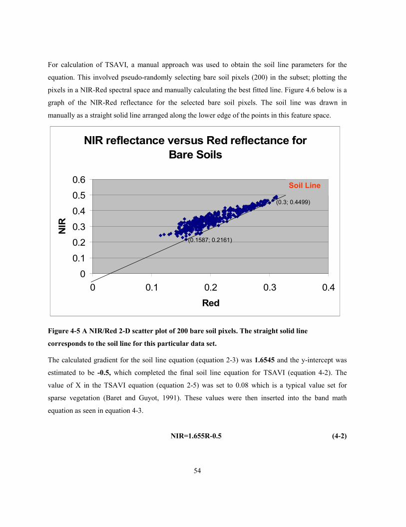
54
For calculation of TSAVI, a manual approach was used to obtain the soil line parameters for the
equation. This involved pseudo-randomly selecting bare soil pixels (200) in the subset; plotting the
pixels in a NIR-Red spectral space and manually calculating the best fitted line. Figure 4.6 below is a
graph of the NIR-Red reflectance for the selected bare soil pixels. The soil line was drawn in
manually as a straight solid line arranged along the lower edge of the points in this feature space.
Figure 4-5 A NIR/Red 2-D scatter plot of 200 bare soil pixels. The straight solid line
corresponds to the soil line for this particular data set.
The calculated gradient for the soil line equation (equation 2-3) was 1.6545 and the y-intercept was
estimated to be -0.5, which completed the final soil line equation for TSAVI (equation 4-2). The
value of X in the TSAVI equation (equation 2-5) was set to 0.08 which is a typical value set for
sparse vegetation (Baret and Guyot, 1991). These values were then inserted into the band math
equation as seen in equation 4-3.
NIR=1.655R-0.5 (4-2)
NIR reflectance versus Red reflectance for
Bare Soils
0
0.1
0.2
0.3
0.4
0.5
0.6
0 0.1 0.2 0.3 0.4
Red
NIR
Soil Line
(0.3; 0.4499)
(0.1587; 0.2161)

55
TSAVI= 1.655)))))*(1.655+(1*(0.08+(-0.5))*(1.655-b3+float(b4))*((1.655
(-0.5)))-float(b3))*(1.655-(b4*((1.655
(4-3)
Where: B3=Red,
B4=NIR
The calculated VI values were confirmed by selecting a pixel within the subsets of the original
Landsat TM image and identifying its corresponding reflectance in the red and NIR bands and
manually calculating the expected NDVI, SAVI and TSAVI.
4.2.2.1.2 Threshold Selection
Threshold selection was done in the continuous gully subset because it best represented the gully
erosion in the study area. The spatial profiler tool in ENVI 4.3 was used to visually select a
vegetation index lower and upper threshold within which pixels values were assigned to soil that is
assumed to be gully erosion. This was done by drawing a transect across ten different locations on the
continuous gully and visually identifying the corresponding value, for each VI. This interactive
process helped identify a range of candidate values that could be used as thresholds to map gullies.
Similar transects were visually evaluated to estimate VI thresholds to test for gully mapping. Once
thresholds were identified for each vegetation index in each subset, they were used to create a gully
mask using a similar technique as applied by Cyr et. al (1995). This mask was then transformed into a
gully map by applying the ISODATA unsupervised classification with a limit of two classes labeled
gullied area and non gullied area. It is important to note that this classification was only used to label
the already created mask, no analysis was run. This process is essentially developing classification
rules to map gullies, for example an associated rule for classifying gullied areas using NDVI would
look similar to the following rule:
If NDVI ≥0.4 then the pixel belongs to gullied area
If NDVI ≤ 0.4 then the pixel belongs to non gullied area
Threshold selection was an optimization process which was run several times, using random values
for each subset, until a maximum accuracy was achieved (maximum kappa statistic) for each
vegetation index. It was assumed that approximately 70% of the gullies in the study area were
continuous gullies, thus the threshold that produced the maximum kappa statistic for the continuous
gully subset was applied to the sub-catchment subset and tested in the discontinuous gully subset.
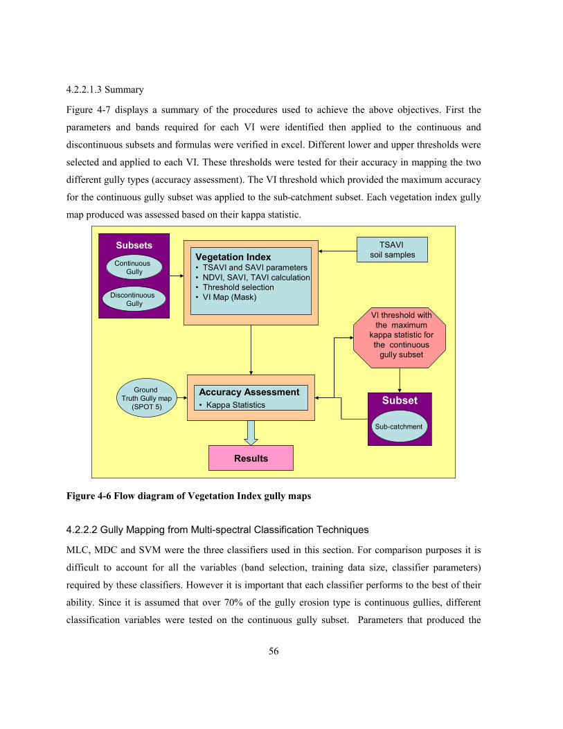
56
4.2.2.1.3 Summary
Figure 4-7 displays a summary of the procedures used to achieve the above objectives. First the
parameters and bands required for each VI were identified then applied to the continuous and
discontinuous subsets and formulas were verified in excel. Different lower and upper thresholds were
selected and applied to each VI. These thresholds were tested for their accuracy in mapping the two
different gully types (accuracy assessment). The VI threshold which provided the maximum accuracy
for the continuous gully subset was applied to the sub-catchment subset. Each vegetation index gully
map produced was assessed based on their kappa statistic.
Ground
Truth Gully map
(SPOT 5)
Vegetation Index• TSAVI and SAVI parameters
• NDVI, SAVI, TAVI calculation
• Threshold selection
• VI Map (Mask)
Accuracy Assessment
• Kappa Statistics
Results
Subset
Sub-catchment
Major
Gully
Continuous
Gully
Discontinuous
Gully
Subsets
VI threshold with
the maximum
kappa statistic for
the continuous
gully subset
TSAVI
soil samples
Figure 4-6 Flow diagram of Vegetation Index gully maps
4.2.2.2 Gully Mapping from Multi-spectral Classification Techniques
MLC, MDC and SVM were the three classifiers used in this section. For comparison purposes it is
difficult to account for all the variables (band selection, training data size, classifier parameters)
required by these classifiers. However it is important that each classifier performs to the best of their
ability. Since it is assumed that over 70% of the gully erosion type is continuous gullies, different
classification variables were tested on the continuous gully subset. Parameters that produced the
57
highest kappa statistic were selected as input parameters for the sub-catchment subset. The objective
of this section is:
• To test the need for image transformation for MLC, MDC and SVM for mapping gullies.
• To test the effect in classification accuracy with different training data sizes
• To determine the SVM parameters for gully mapping using Landsat TM.
• To determine the classification accuracy, using the kappa statistic, of the gully maps
produced from MLC, MDC, and SVM in the continuous and discontinuous and sub-
catchment subsets.
4.2.2.2.1 Principal Component Analysis
A principal component analysis (PCA) was run to ensure that the maximum accuracy for mapping
gullies was achieved with conventional classification algorithms. PCA is a process that compresses
the information content from a number of bands into a few principal components which are
uncorrelated and easier to interpret (Jensen, 2005). It has proven to increase classification accuracies
of conventional classification algorithms (Wu and Linders, 2000).
PCA was run on the Landsat TM discontinuous and continuous subset and two tests were run using
the first 5 PC bands (Test 3) and first 4 PC bands (Test 4). The last principal components were
disregarded because they contained most of the noise in the image. This aim was to assess whether
the classification accuracies improved when applied to an uncorrelated image with less noise (PCA
image) rather than the original preprocessed Landsat TM image which is assumed to carry more
noise.
4.2.2.2.2 Training
Although it is important to consider the classifier when choosing the training data, for comparative
purposes, the same training data was used for each classifier. Two classes of training data were used
in this study: gully and non gully. The number of pixels chosen for each class was based on Jensen
(2005) general rule that states “the number of pixels used for the training data from n bands should be
>10n.” The total number of Landsat TM bands used were six, thus the number of training pixels
selected was >60.
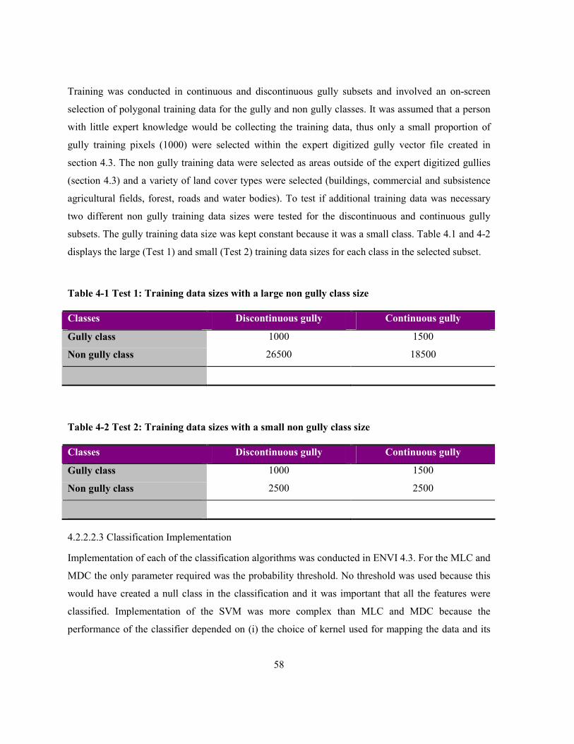
58
Training was conducted in continuous and discontinuous gully subsets and involved an on-screen
selection of polygonal training data for the gully and non gully classes. It was assumed that a person
with little expert knowledge would be collecting the training data, thus only a small proportion of
gully training pixels (1000) were selected within the expert digitized gully vector file created in
section 4.3. The non gully training data were selected as areas outside of the expert digitized gullies
(section 4.3) and a variety of land cover types were selected (buildings, commercial and subsistence
agricultural fields, forest, roads and water bodies). To test if additional training data was necessary
two different non gully training data sizes were tested for the discontinuous and continuous gully
subsets. The gully training data size was kept constant because it was a small class. Table 4.1 and 4-2
displays the large (Test 1) and small (Test 2) training data sizes for each class in the selected subset.
Table 4-1 Test 1: Training data sizes with a large non gully class size
Classes Discontinuous gully Continuous gully
Gully class 1000 1500
Non gully class 26500 18500
Table 4-2 Test 2: Training data sizes with a small non gully class size
Classes Discontinuous gully Continuous gully
Gully class 1000 1500
Non gully class 2500 2500
4.2.2.2.3 Classification Implementation
Implementation of each of the classification algorithms was conducted in ENVI 4.3. For the MLC and
MDC the only parameter required was the probability threshold. No threshold was used because this
would have created a null class in the classification and it was important that all the features were
classified. Implementation of the SVM was more complex than MLC and MDC because the
performance of the classifier depended on (i) the choice of kernel used for mapping the data and its

59
parameters, and (ii) the choice of user-defined parameters C (which controls the penalty associated
with misclassifications) (Boyd et al., 2006).
Selecting the most accurate parameters for the SVM was critical in this study because inappropriately
selected parameters could produce very low accuracies and thus inadequate gully mapping results.
Four main kernels are discussed in the literature- linear, polynomial, radial basis function (RBF),
sigmoid- however it is difficult to distinguish which one gives the best generalization for mapping
gullies. Furthermore there is little guidance in literature on the choice of the kernel and the ideal
parameters to use (Mantero and Moser, 2005; Pal and Mather, 2005). Therefore in this study the four
different kernels were tested on the continuous gully because it was assumed to represent most of the
sub-catchment area and it was small enough to reduce processing time. The kernel that produced the
highest kappa statistic, with default values, was then used to test a range of values for parameters C
(varying from 1-5000) and γ (0-60). The parameters that produced the highest accuracy for the
continuous gully subset were then used to classify the discontinuous and sub-catchment gully subset.
4.2.2.3 Summary of Classification Algorithm Tests
The classification gully mapping procedures involved in this study required five main tests which are
listed below and illustrated in Figure 4-8. Test 1-6 were conducted using both the discontinuous gully
and the continuous gully subset whereas the SVM parameter tests were only conducted on the latter.
1. Training data test
• Large training data size (Test 1)
• Small training data size (Test 2)
2. SVM Parameter tests
• kernel selection
• C parameter
• γ parameters
3. Principal component analysis
• Principal components 1-4 (Test 3)
• Principal components 1-5 (Test 4)
4. Sub-catchment subset (test for regionalization)
• Apply classification variables that produced the maximum kappa statistic for continuous
gully subset, to the sub-catchment subset (Test 5)
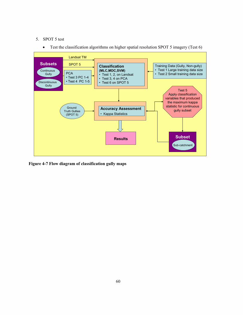
60
5. SPOT 5 test
• Test the classification algorithms on higher spatial resolution SPOT 5 imagery (Test 6)
Ground
Truth Gullies
(SPOT 5)
Classification (MLC,MDC,SVM)
• Test 1, 2, on Landsat
• Test 3, 4 on PCA
• Test 6 on SPOT 5
Accuracy Assessment
• Kappa Statistics
Results
PCA
• Test 3 PC 1-4
• Test 4 PC 1-5
Subsets
Continuous
Gully
Discontinuous
Gully
Subset
Sub-catchment
Training Data (Gully, Non-gully)
• Test 1 Large training data size
• Test 2 Small training data size
Test 5
Apply classification
variables that produced
the maximum kappa
statistic for continuous
gully subset
Landsat TM
SPOT 5
Figure 4-7 Flow diagram of classification gully maps

61
Chapter 5
Results
5.1 Vegetation Indices
The spatial profile tool in ENVI 4.3 helped compare the range of values for each vegetation index
(Figure 5-1). Figure 5-1 displays graphs with extracted NDVI, SAVI and TSAVI pixel values (y-axis)
of different transects (x-axis) crossing over selected land cover types. The yellow arrow indicates the
location of the particular land cover type on the transect. The general range of the VIs was between
+1 to 0 with values close to zero being bare soil and values close to one representing very healthy
vegetation. There were some cases of negative values for NDVI and SAVI which were located in
areas of deep water; however TSAVI had no negative values. The trend for each VI was slightly
similar, TSAVI produced generally higher values, except in healthy vegetated areas (agriculture and
wetlands) where NDVI was higher, then NDVI ranked second for other land cover types, followed by
SAVI which produced much lower values. Data from vegetated areas, for example agriculture,
wetlands and grasslands, yielded high VI values due to high near-infrared and low red or visible
reflectance (Jensen, 2005). Water produced low VI values (NDVI=0.1, SAVI=0.08 and TSAVI=0.45)
because it has a higher reflectance in the red or visible bands than the NIR (top right of Figure 5-1).
SAVI results were similar to NDVI, except the values were slightly lower. For NDVI and SAVI bare
soil areas coincided with low positive values close to zero because bare soil generally has similar
reflectance in the NIR and red or visible bands (Jensen, 2005). The bare soil values were similar to
that of gullies (Figure 5-3 and Figure 5-4). TSAVI values were also low for bare soil compared to
other land cover types but values were close to 0.5 rather than zero.

62
NDVI
TSAVI
SAVI
NDVI
TSAVI
SAVI
NDVI
TSAVI
SAVI
NDVI
TSAVI
SAVI
Grassland
Agricultural
WaterWetland
Figure 5-1 Spatial profile of NDVI, SAVI and TSAVI values across different land cover types in
the study area
5.1.1 Vegetation Index Threshold
More specific to this study was the range of NDVI, SAVI and TSAVI values within a gully system.
Figure 5-2 displays a Landsat TM false colour composite of the continuous gully subset and the three
corresponding calculated vegetation index results.

63
NDVI SAVI TSAVI
False colour composite
Figure 5-2Top image is a false colour composite of the continuous gully subset. Bottom (left to
right) are the NDVI, SAVI and TSAVI results for the continuous gully subset.
Figure 5-3 is a gully with a transect (A-B-C) across its channel (B), displayed is a false colour image
made up of TSAVI, NDVI and SAVI entered into the red, green and blue colour guns, respectively.
The corresponding graph illustrates the VI values (y-axis) of extracted pixel along the transect (A-B-
C), that passes from an area of non gully (A) to gully (B) to non gully (C) (solid line A-C in gully
image).

64
AC
Gully Transect Spatial Profile
NDVI
TSAVI
SAVI
Gully
BCA B
Figure 5-3 Spatial profile of NDVI, SAVI, TSAVI values across a gully
Figure 5-4 displays five transect graphs extracted along a continuous gully channel, using the same
method in Figure 5-3. It can be observed that the VI values at the base of the gully are generally low
for NDVI, SAVI and TSAVI, compared to no gully areas. The NDVI, SAVI, TSAVI values for the
base of the gully (B) are approximately 0.3, 0.27 and 0.5 respectively. These low VI values could be
attributed to the moisture conditions of the gully bottom (Vrieling et al., 2008). The observed VI
values have a similar trend across the gully channel, with NDVI values generally range between
SAVI and TSAVI values. Mapping of gullies using Landsat TM seems to be feasible following the
comparison of these VI values with surrounding areas.

65
NDVI
NDVINDVI
NDVI
TSAVITSAVI
TSAVI
TSAVI
NDVI
SAVI
SAVI
SAVI
SAVI
SAVI
TSAVI
Gully Gully
Gully
Gully
Gully
Figure 5-4 Spatial profiles of VI values across transects along a continuous gully
The selected lower threshold for gully mapping using NDVI and SAVI was zero and for TSAVI 0.41.
Table 5-1 lists the top five kappa statistics achieved with the tested upper VI thresholds for the
continuous gully subset. Figure 5-5 displays the kappa statistics trend for each tested VI threshold.
The selected upper thresholds used to represent each VI were the ones that produced the maximum
kappa statistic (bold values in Table 5-1). The chosen thresholds used to classify the image can be
explained using the following rules:
If 0 ≤ NDVI ≤ 0.40 then pixel belongs to gullies, else non gully
If 0 ≤ SAVI ≤ 0.274 then pixel belongs to gullies, else non gully
If 0.41 ≤ TSAVI ≤ 0.55 then pixel belongs to gullies, else non gully

66
Table 5-1 Tested upper VI thresholds that produced the highest kappa statistic for gully
mapping in the continuous gully subset
Tested Upper Threshold The top five kappa statistics
0 ≤ NDVI 0 ≤ SAVI 0.41 ≤ TSAVI
0.27 0.4903
0.273 0.4949
0.274 0.4961
0.275 0.4958
0.280 0.4928
0.380 0.5330
0.390 0.5474
0.400 0.5555
0.405 0.5541
0.410 0.5534
0.530 0.4485
0.540 0.5373
0.550 0.5580
0.555 0.5569
0.560 0.5492

67
Tested Upper Limit Thresholds for VI
0.00
0.10
0.20
0.30
0.40
0.50
0.60
0.25
0.27
0.27
0.28
0.30
0.40
0.41
0.53
0.55
0.56
0.57
0.58
0.60
Upper Limit Threshold
Kap
pa
Sta
tisti
c
0 ≤ NDVI
0 ≤ SAVI
0.41 ≤ TSAVI
Figure 5-5 A graph of the tested upper thresholds for each vegetation index
5.1.2 Gully Maps from Vegetation Indices
Figure 5-6 displays the VI gully maps produced when the selected threshold values were applied to
the continuous gully subset. TSAVI performed the best with an accuracy of 0.5580 followed by
NDVI, with an accuracy of 0.555, and last SAVI, with an accuracy of 0.496.
NDVI Kappa = 0.555 TSAVI Kappa = 0.5580SAVI Kappa = 0.496
Co
nti
nu
ou
s G
ull
y
Gullies No gullies
Figure 5-6 VI continuous gully map with kappa statistic results
Figure 5-7 displays the VI gully maps produced when the selected threshold values were applied to
the discontinuous gully subset. The results achieved were very low compared to the continuous gully
map. SAVI had the highest kappa statistic of 0.2216, followed by NDVI with an accuracy of 0.2088
and TSAVI with accuracy of 0.1793.

68
Dis
co
nti
nu
ou
s G
ullie
s
Gullies No gullies
NDVI Kappa = 0.2088 SAVI Kappa = 0.2216 TSAVI Kappa = 0.1793
Figure 5-7 VI discontinuous gully map with VI kappa statistic results
Table 5-2 lists the VI accuracies produced when the selected threshold values were applied to the sub-
catchment gully subset. NDVI had the highest kappa statistic of, 0.3616, followed by TSAVI with
0.3337 and SAVI with 0.2997. The maps produced were not very clear for representation in this
document; however results are discussed in terms of the distribution of error in section 5.1.5.1
Table 5-2 VI kappa statistic results for the Sub-catchment gully map
VI Sub-catchment
NDVI 0.3616
SAVI 0.2997
TSAVI 0.3337
5.1.3 Gully Map Accuracy Assessment from Vegetation Indices
Figure 5-8 and Table 5-3 is a summary of the kappa statistic results for the three VI subset maps. The
continuous gully subset was mapped with the highest kappa statistic across all the vegetation indices
ranging around 0.5, followed by the sub-catchment scale around 0.3 and the discontinuous gullies
around 0.2. All the indices performed better at identifying the continuous gully system, than their
performance in the other two subsets. TSAVI produced the most accurate continuous gully map
(0.558), SAVI produced the most accurate discontinuous gully map (0.2216) and NDVI ranked first
at mapping gullies in the sub-catchment subset (0.3616).

69
Vegetation Index Accuracy Assessment
0
0.1
0.2
0.3
0.4
0.5
0.6
Discontinuous Continuous sub-catchment
Landsat TM gully subsets
Kap
pa s
tati
sti
cs
NDVI
SAVI
TSAVI
Figure 5-8 Kappa statistics graph comparing the VI results for each gully subset
Table 5-3 VI kappa statistic results for gully mapping in each subset
VI Discontinuous gully Continuous gully sub-catchment
NDVI 0.2088 0.5508 0.3616
SAVI 0.2216 0.4961 0.2997
TSAVI 0.1793 0.558 0.3337
5.1.4 Discussion
Although individual studies have compared the use of VI based on their effectiveness to estimate and
detect water erosion (Baugh and Groeneveld, 2006; Cyr, et al., 1995); no comprehensive study has
attempted to compare the accuracy of VI for mapping gullies. Cyr et al. (1995) performed a
comparative study of vegetation indices derived from the ground and from satellite images, to find the
best index for estimating soil protection against water erosion. Whereas Baugh and Groeneveld,
(2006) compared fourteen VI for mapping erosion.
With the potential of the soil line indices (SAVI and TSAVI) being better at identifying vegetation, it
is disappointing that these indices did not out-perform NDVI for gully mapping because most of the
vegetation would be identified and masked out; NDVI had the highest accuracy over the sub-
catchment subset at 0.3616 It is possible that NDVI was more accurate in the sub-catchment subset
because the soil line for the whole area was not that much different than NDVI assumed soil line
70
(Lawrence and Ripple, 1998). The TSAVI and SAVI soil line parameters were probably not
exemplary for the sub-catchment subset soil line because they were obtained in the continuous gully
subset. For TSAVI, soil line parameters may have been obtained from the same soil type. Therefore
when the index was applied to the sub-catchment and discontinuous gully subsets, a majority of the
soils may have been different. Although SAVI parameter L which was assumed at 0.5 is said to be
most ideal for minimizing soil variations in sparse vegetation (Huete, 1988), it may not have been the
ideal parameter value for the type of vegetation in the study area. It is also possible that most of the
gullies in the study region had vegetation within them and if this is the case the soil line indices
performed successfully, at identifying vegetation, to the extent that the vegetation within the gullies
was removed resulting in a lower kappa statistic because of errors of commission. This highlights the
importance of ancillary data, such as soil and rainfall data, when using remote sensing to draw
conclusions on areas where one has little knowledge. Although substantial success has been achieved
through the use of soil adjusted vegetation indices for the prediction of vegetation variables, this
study proves that simple NDVI achieves equivalent or better results without much additional effort
for mapping gullies.
Although TSAVI performed the best in the continuous gully subset, with an accuracy of 0.5580 it is
recommended that NDVI still be selected, because of the computational cost of the TSAVI soil line
parameters. TSAVI performed well in the continuous gully subset because the soil line parameters
were modeled to the area. But NDVI was only 0.0072 less accurate than TSAVI, which is not
significantly different considering the amount of time and additional information necessary (soil line
parameters) to calculate TSAVI.
While NDVI performed the best overall, some of the major limitations are its sensitivity to
atmospheric conditions, soil, and view/sun angle conditions (Dash et al., 2007). The atmospheric
conditions lower the NDVI of vegetated areas and in areas where the vegetation is on darker soil
substrates, the NDVI produces higher vegetation index values (Huete, 1988), as shown in the wetland
graph in Figure 5-1. An additional limitation is that the NDVI is insensitive to very high and very low
chlorophyll content, which is an important biochemical property that varies with vegetation type
(Gilabert, et al. 2002). Lastly when compared across different soil types, NDVI has been found to be
affected (Huete, 1988) especially during open plant canopy periods. All these limitations restrict the
NDVI quantitative capabilities to characterize the vegetated surface (Huete, et al. 1992) and therefore

71
a limitation in gully erosion mapping. But given the presented challenges of trying to assume the
vegetation type for SAVI and difficulties in obtaining soil line parameters for calculating TSAVI,
NDVI is still the final recommended technique for mapping gullies in South Africa.
5.1.5 Vegetation Index Choice for Gully Mapping – some guidelines
This study has successfully compared three VI for gully mapping in KZN. The results presented
confirm that NDVI and TSAVI can be used to map a continuous gully with a moderate level of
agreement using little knowledge when compared to traditional methods of gully mapping. Overall,
NDVI proved to be more accurate at the sub-catchment level than TSAVI, which was ideal for
identifying a continuous gully system and SAVI was best for a discontinuous gully system.
Explanation for the distribution of error (omission and commission) can only be validated with
additional information such as rainfall patterns prior to image acquisition and the distribution of soil
types. For improvements in TSAVI, it is recommended that the selected soil patches be random
across soil types, this will ensure that the VI parameters are generalized for the whole study region.
When little is known about the study region and little expert knowledge is available, NDVI is
recommended to identify erosion.
The experiments carried out in this study can be used to form a number of guidelines that can greatly
facilitate the use of VI for gully erosion mapping using Landsat TM. The list of guidelines presented
is ranked from highest to lowest and are given as follows:
A. Time required
1. TSAVI – slow process involved in selecting bare soil pixels for soil line equation.
2. SAVI – average amount of time spent on calculating the formula.
3. NDVI – quick, because model was already built in the ENVI 4.3 program
B. Expert knowledge required
1. TSAVI - required extensive expert knowledge, for collecting bare soil pixels, calculation was
very complex
2. SAVI – average
3. NDVI - easiest, required little knowledge
C. Accuracy for mapping continuous gullies
1. TSAVI - high

72
2. NDVI – medium
3. SAVI - low
D. Accuracy for mapping discontinuous gullies
1. SAVI - high
2. NDVI - high
3. TSAVI - low
E. Accuracy in mapping sub-catchment level
1. NDVI – high
2. TSAVI - medium
3. SAVI - low
5.2 Gully Mapping Results from Multi-spectral Classification Techniques
5.2.1 Support Vector Machine Parameters
Appendix E is a list of the tested SVM parameter and the following are the selected values:
• RBF was the chosen kernel function which performed the best (0.5794) compared to the
other three kernels. This kernel is known for its capability to separate classes that are not
linearly separable with less numerical difficulties (Hsu, et al. 2008).
• The chosen value of C was 1000 which provided the highest kappa statistic of 0.601. Values
were not tested above 1000 because increasing the penalty parameter would increase the cost
of misclassifying points and would create a model that would not generalize well.
• The γ parameter is a kernel specific parameter that controls the width of the RBF kernel. The
chosen value for γ was 0.167, which concurred with previously tested γ values which
typically ranged between 0 and 1 (Joachims, 1998; Vapnik, 1995). Haung et al. (2002)
provides details on the effect of γ on the decision boundary.
5.2.2 Training Sample Size
Table 5-4 is the classification accuracy results for a large and small non gully training data size (test 1
and test 2) for the discontinuous and continuous gully system. The values in brackets indicate the
change in accuracy when a smaller training data set was used (↓ = decrease and ↑= increase). MDC
performed the best within test 1 with a kappa statistic of 0.353 for the discontinuous gully subset and
0.5719 for the continuous gully subset. All classifications improved after test 2 with the most

73
significant increase in accuracy produced by SVM, in both continuous and discontinuous gully
subset, which increased by 0.0227 and 0.0363, respectively. However MDC was the most accurate in
mapping gullies within test 2 in the discontinuous gully subset producing an accuracy of 0.374.
Table 5-4 Classification kappa statistics results using different training data sizes
Tests Discontinuous Gully Continuous Gully
Test 1: Large Sample Size
MLC 0.3155 0.4265
MDC 0.353 0.5719
SVM 0.3365 0.5647
Test 2: Small Sample Size
MLC 0.3516 (↑0.0361) 0.5196 (↑0.0931)
MDC 0.3740 (↑0.0210) 0.5804 (↑0.0085)
SVM 0.3592 (↑0.0227) 0.6010 (↑0.0363)
5.2.3 Principal Component Analysis
Table 5-5 are the kappa statistic results obtained after applying the classifiers to two PCA images one
with the first five PC (Test 3) and the other the first four PC (Test 4). The values in brackets, in Table
5-5, indicate the amount of increase compared to the small sample size classification (Test 2). The
PCA increased the accuracy of MLC and MDC in both PC combinations, except the MDC test 4 in
the discontinuous gully subset which decreased (↓0.0100). The PCA test 3 had a more significant
increase than test 4 for MLC and MDC. MLC had the most significant increase in accuracy in these
two tests with an accuracy increase of 0.0609 in the continuous gully subset. The SVM classifier
experienced a decrease in accuracy using PCA. The bold values in Table 5-4 and 5-5 are the selected
accuracies used to represent each subset gully maps and were the set procedures that were applied to
the sub-catchment gully subset.

74
Table 5-5 Classification kappa statistics results with selected PCA bands
Tests Discontinuous Gully Continuous Gully
Test 3: PCA 1_2_3_4_5
MLC 0.3573 (↑0.0057) 0.5805 (↑0.0609)
MDC 0.3598 (↑0.0068) 0.5835 (↑0.0031)
SVM 0.3569 (↓0.0023) 0.5842 (↓0.0168)
Test 4: PCA 1_2_3_4
MLC 0.3540 (↑0.0024) 0.5803 (↑0.0607)
MDC 0.3640 (↓0.0100) 0.5830 (↑0.0026)
SVM 0.3575 (↓0.0017) 0.5854 (↓0.0156)
5.2.4 Gully Maps from Multi-spectral Classification Techniques
With reference to Figure 5-9, visual comparison of SVM produced a continuous gully map that was
less speckled and the gully was more defined than in the other MLC and MDC continuous gully
maps. It is challenging to visually assess the classifiers performance in the discontinuous gully subset
and is actually insignificant because of the low accuracy achieved.

75
MLC Kappa = 0.5805 SVM Kappa = 0.601MDC Kappa = 0.5835C
on
tin
uo
us
Gu
lly
Dis
co
nti
nu
ou
s G
ullie
s
No gullyGully
MLC Kappa = 0.3573 SVM Kappa = 0.3592MDC Kappa = 0.3598
Figure 5-9 Classification gully maps with kappa statistic results
5.2.5 Gully Map Accuracy Assessment from Multi-spectral Classification Techniques
Table 5-6, Figure 5-10 and summarizes the maximum kappa statistics achieved for the continuous and
discontinuous subsets as well as the results for the sub-catchment gully subset (Test 5). Figure 5-10
suggests that the continuous gully subset was the only one that produced a high accuracy for all three
classifiers. All three classifiers produced similar results for the discontinuous gully subset with a low
accuracy of approximately 0.36. Both MLC and MDC poorly classified the sub-catchment gully
subset with a low accuracy of 0.2589 and 0.2499 respectively; however, the SVM classified sub-
catchment with a higher accuracy (0.4063), compared to its performance in the discontinuous gully
subset at (0.3592).

76
Table 5-6 Classification kappa statistics results for mapping gullies in subsets
Algorithms Discontinuous Gully Continuous gully Sub-catchment gully
MLC (Test 3) 0.3573 0.5805 0.2589
MDC (Test 3) 0.3598 0.5835 0.2499
SVM 0.3592 0.601 0.4063
Kap
pa s
tati
sti
c
Figure 5-10 Classification kappa statistic results for mapping gullies in each subset
5.2.5.1 Results Using Multi-spectral Classification Techniques on SPOT 5 Imagery
Table 5-7 are the results obtained when the classifiers were applied to SPOT 5 data, the values in
brackets are the differences in value from Table 5-6. All the classification algorithms performed
poorly in the discontinuous and continuous gully subsets values. MLC and MDC had a more
significant decrease in accuracy, for both subsets compared to SVM.
Table 5-7 Classification kappa statistics results with SPOT 5
Test 6 Discontinuous Gully Continuous Gully
MLC 0.2291 (↓-0.1282) 0.4100 (↓-0.1705)
MDC 0.2308 (↓-0.129) 0.4717 (↓-0.1118)
SVM 0.3042 (↓-0.055) 0.5331 (↓-0.0679)

77
5.2.6 Discussion
The following discussion addresses the performance of the classificaiton algorithms for mapping
gullies, in terms of training data separability and size, and the algorithm decision boundaries. These
differences build the case for the selection of the most ideal classifier for gully mapping in South
Africa.
5.2.6.1 Issue of Class Spectral Separability
The main obstacle in achieving high accuracies of the gully erosion maps derived from medium
resolution (Landsat TM) satellite data is the heterogeneous nature of the gullies because they can
consist of water, vegetation, and bare soil (section 2.3.2.2). The inherently high heterogeneity of
gullies made it challenging for traditional classifiers to detect gullies because features that existed in
the gully class also existed in the non gully class. This is an issue of class spectral separability.
The issue of spectral separability between the gully and the non gully class can be observed in Figure
5-11. This image displays the gully and non gully training data from Test 2, projected in a five band
feature space. It illustrates the complexity of identifying a boundary that best separates the classes
because the gully training data, indicated as green, and the non gully training data, indicated as
yellow, both have overlapping regions in feature space. This area of over lap (fuzzy area) illustrates
the region where features that are present in the gully class are also present in the non gully class.
Figure 5-11 The Gully and Non Gully training data in a five band feature space
78
5.2.6.2 Training Data Size
Training data size is related to the “number of spectral bands, to which statistical properties are to be
estimates, the number of those statistical properties, and the degree of variability present in the class”
(Mather, 2004). Research has found a positive relationship between the size of the training set and
classification accuracy for various classifiers (Foody and Arora, 1997; Foody and Mathur, 2004a).
However acquiring large training sets is costly and time consuming and therefore may not be ideal for
mapping gullies in South Africa. Interestingly enough this study has proven that a smaller training
data size (Test 2) for the non gully class is more suitable for mapping gullies than a larger training
data size (Test 1) (Table 5-4). In the following paragraph addresses the possible reasons for these
results in hopes to obtain an ideal algorithm for mapping gullies in South Africa.
Some insight is gained into why the classifiers are producing significantly different accuracy results
with different training data sizes, by looking at how the classifiers work. MLC and MDC are based on
statistical descriptions of the classes generated from the training data (Mathur and Foody, 2008). It
would be expected that these two classifiers would improve with a larger training data set because all
classes would be exhaustively defined (Sanchez-Hernandez et al., 2007b). Although a large training
data for the non gully class does capture all the land cover types in the area; the multimodality of the
class defies the MLC assumptions of normality thus feeding to the low accuracy results. MLC had
the most significant increase in accuracy using a smaller training data size (Table 5-4), most likely
because the training data size allowed for greater separability between the two classes. On the other
hand, MDC was not significantly affected by the change in training data size (from Test 1 to Test 2)
because it does not take into account possible data multimodality (Lai et al., 2002), such as the non
gully class. MDC assumes all class covariance’s are equal (Richards and Jia, 2006) and bases its
classification decisions on the mahalanobis distance rather than the probability of a pixel being in a
class. This assumption of equal covariance’s reduced the spectral complexity within the classes and
allowed for the decision boundaries to be more concise. In doing so MDC is less affected by outliers
in the training data because an unknown pixel is classified based on the distance of an uknown pixel
from the center of a class ellips (i.e mean) divided by the width of the ellipsoid in the direction of the
unknown pixel. This explains why MDC did not increase significantly when the training data size
was reduced.
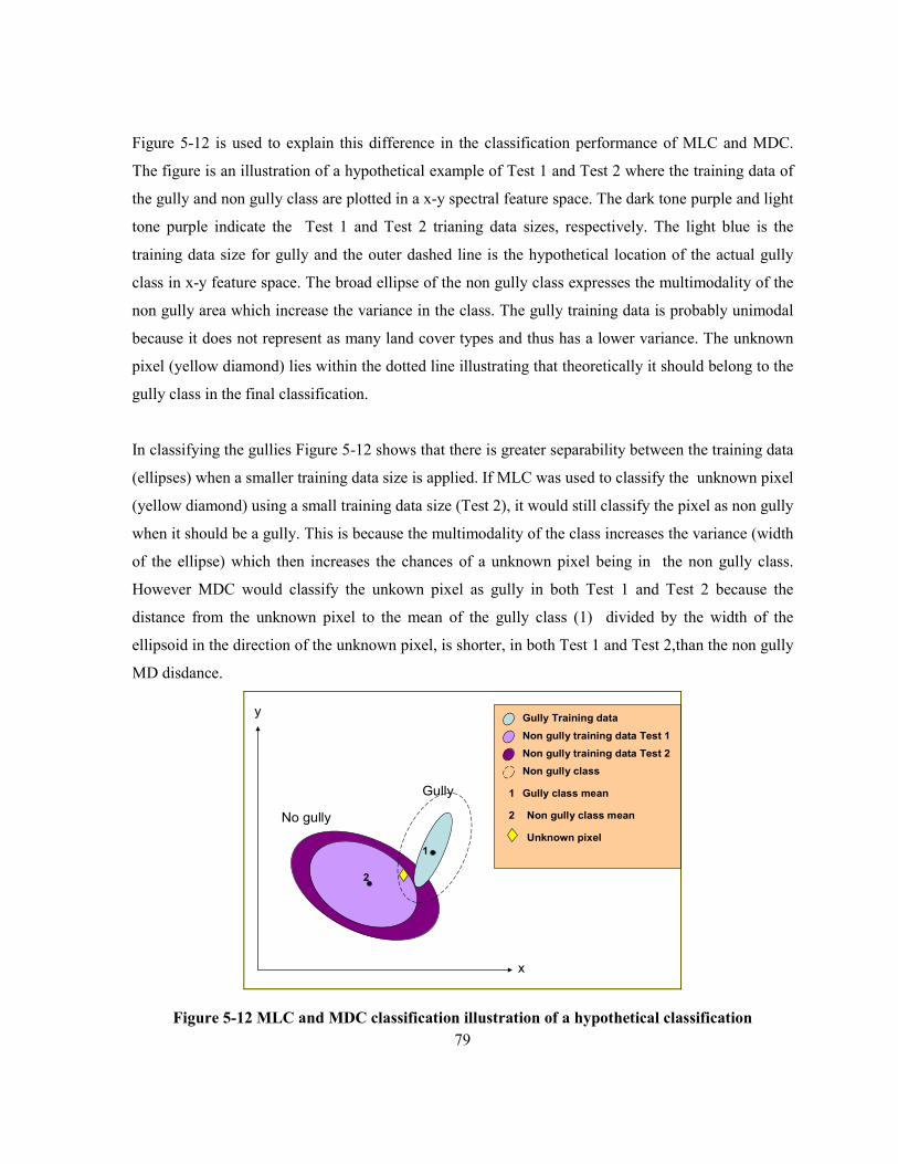
79
Figure 5-12 is used to explain this difference in the classification performance of MLC and MDC.
The figure is an illustration of a hypothetical example of Test 1 and Test 2 where the training data of
the gully and non gully class are plotted in a x-y spectral feature space. The dark tone purple and light
tone purple indicate the Test 1 and Test 2 trianing data sizes, respectively. The light blue is the
training data size for gully and the outer dashed line is the hypothetical location of the actual gully
class in x-y feature space. The broad ellipse of the non gully class expresses the multimodality of the
non gully area which increase the variance in the class. The gully training data is probably unimodal
because it does not represent as many land cover types and thus has a lower variance. The unknown
pixel (yellow diamond) lies within the dotted line illustrating that theoretically it should belong to the
gully class in the final classification.
In classifying the gullies Figure 5-12 shows that there is greater separability between the training data
(ellipses) when a smaller training data size is applied. If MLC was used to classify the unknown pixel
(yellow diamond) using a small training data size (Test 2), it would still classify the pixel as non gully
when it should be a gully. This is because the multimodality of the class increases the variance (width
of the ellipse) which then increases the chances of a unknown pixel being in the non gully class.
However MDC would classify the unkown pixel as gully in both Test 1 and Test 2 because the
distance from the unknown pixel to the mean of the gully class (1) divided by the width of the
ellipsoid in the direction of the unknown pixel, is shorter, in both Test 1 and Test 2,than the non gully
MD disdance.
Gully
No gully
2
x
yGully Training data
Non gully training data Test 2
Non gully class
1
2
Gully class mean
Non gully class mean
Unknown pixel
Non gully training data Test 1
1
Figure 5-12 MLC and MDC classification illustration of a hypothetical classification

80
SVM does not rely explicitly on the dimensionality of the training data but uses pattern recognition,
regression, and density estimation in high-dimensional spaces to separate the classes (Vapnik, 1998).
Visual assessment of Figure 5-9 suggests that the SVM has mapped the continuous gully subset more
accurately than the conventional classifiers. More importantly, the results in Table 5-4 prove that
SVM can still produce higher accuracies than MLC and MDC even with smaller training data. This is
because SVM is non parametric and only uses the support vectors which lie in the region where the
classes meet (Foody and Mathur, 2006) and not the whole training data set. Thus SVM maximizes on
the complexity of the classes at the boundary and is unaffected by the within class variance. These
results mean that application of SVM for gully mapping requires less time, effort and expert
knowledge required in training on the classes that are of no interest (Foody et al., 2006).
5.2.6.3 Principal Component Analysis
The Principal component analysis was used to test the need for image transformation by the
classifiers. The results show that using PCA increased the accuracy for MLC and MDC in Test 3 but
decreased the accuracy for SVM, but SVM still produced higher accuracies (Table 5-5). The
obtained results confirm the strong superiority of SVMs over the other classifiers even in lower
dimensional feature spaces (Table 5-5). Greater efforts could be put in place, in this analysis, to
increase the accuracy however this can be very time-consuming. The bottom line is that SVM is not
affected by the presence of noise in an image whereas conventional classifiers are. SVM can then be
used without any additional expert knowledge and time needed to run an image transformation; thus it
is applicable for gully erosion mapping in South Africa.
5.2.6.4 Algorithm Time Requirements
The training speeds of the three classifiers were substantially different. In all cases training the MLC
and the MDC did not take more than a few minutes on an IBM thinkPad workstation, while training
the SVM took hours and in some cases days, especially when the training data was large. The SVM
also had the greatest challenge when classifying discontinuous gullies which took three hours. The
long computation time required by SVM expresses the difficulties encountered by the SVM in
identifying a separation between the two classes (Huang et al. 2002; Melgani and Bruzzone, 2004).
The training speeds of these algorithms were affected by the size of the study area, with the sub-
catchment subset taking the longest. Although SVM did require a longer computational time during

81
the process, the removed need for PCA and the higher accuracies across all the subsets still make
SVM superior.
5.2.6.5 SPOT 5 Imagery for Gully Mapping
The classification algorithm test on SPOT 5 imagery (Test 6) was conducted to identify the need for
higher resolution imagery for gully mapping. It would be expected that as the spatial resolution
increases, so the amount of spatial variation, and thereby, the amount of information revealed about
the gullies would increase (Atkinson and Tate, 1999), but with SPOT this is not the case. The
classification results in Table 5-7 (pg 81) show that medium resolution Landsat TM data imagery out
performed the higher resolution SPOT5 imagery for mapping gullies using all classifiers in the
continuous and discontinuous subset. One would have expected that the SPOT image would produce
a more accurate classification because of the finer spatial resolution; however it appears that the
spectral resolution of Landsat TM was more important for identifying the gullies. This is probably
due to the spectral variability within the gullies as explained in section 2.3.2.2., gullies can be
composed of water, bare soil and vegetation. The heterogeneity of the gully makes it difficult for the
classifiers to identify the gullies if less spectral information is provided as in the case of SPOT 5
which only provides 3 spectral bands. However, while the Landsat TM image classification retains
more information than the SPOT classification (as evident in the kappa statistics), the resultant
predictions still display a large degree of uncertainty.
5.2.7 Multi-Spectral Classification Algorithm Choice – some guidelines
Although the methods presented vary in complexity the study represents some of the inputs, issues
and potential of selecting a classifier for gully mapping. Semi-automatic gully detection is very
challenging due to the variability in appearance of the gullies and surrounding terrain. This study has
shown that using state-of-the-art learning algorithms, which have worked well in other pattern
recognition and vision problems, is successful in increasing the detection accuracy of gullies. The
best result achieved from the SVM was the classification of the continuous gully system with an
accuracy of 0.601. Although the computational time for running SVM was greater than the MLC and
MDC, the processing time of SVM was still less than a traditional gully mapping method. The
presented results can be summarized by the following guidelines:
82
A. Time required
1. SVM – slow process involved in running the algorithm.
2. MLC – average amount of time spent training data collection.
3. MDC – quickest
B. Expert knowledge required
1. SVM - required extensive expert
2. MLC – average
3. MDC - easiest, required little knowledge
C. Accuracy for mapping continuous gullies
1. SVM - high
2. MDC – medium
3. MLC - low
D. Accuracy for mapping discontinuous gullies
1. SVM - high
2. MDC - medium
3. MLC - low
E. Accuracy in mapping sub-catchment level
1. SVM – high
2. MDC - medium
3. MLC – low
F. Accuracy with SPOT data for mapping continuous and discontinuous gullies
1. SVM – high
2. MDC – medium
3. MLC – low
5.3 Summary of Results
If we assess these results based on Landis and Koch (1977) characterization of kappa statistics where:
a value greater than 0.80 represents strong agreement, a value between 0.40 and 0.80 represents
moderate agreement, and a value below 0.40 represents poor agreement, then most of the continuous
gully system results performed are reputable as they are within the moderate level of agreement.
Only the sub-catchment subset result for SVM (0.4063) lies within this category. Thus Landsat TM
combined with SVM can be used to produce a gully erosion map at a sub-catchment scale with a
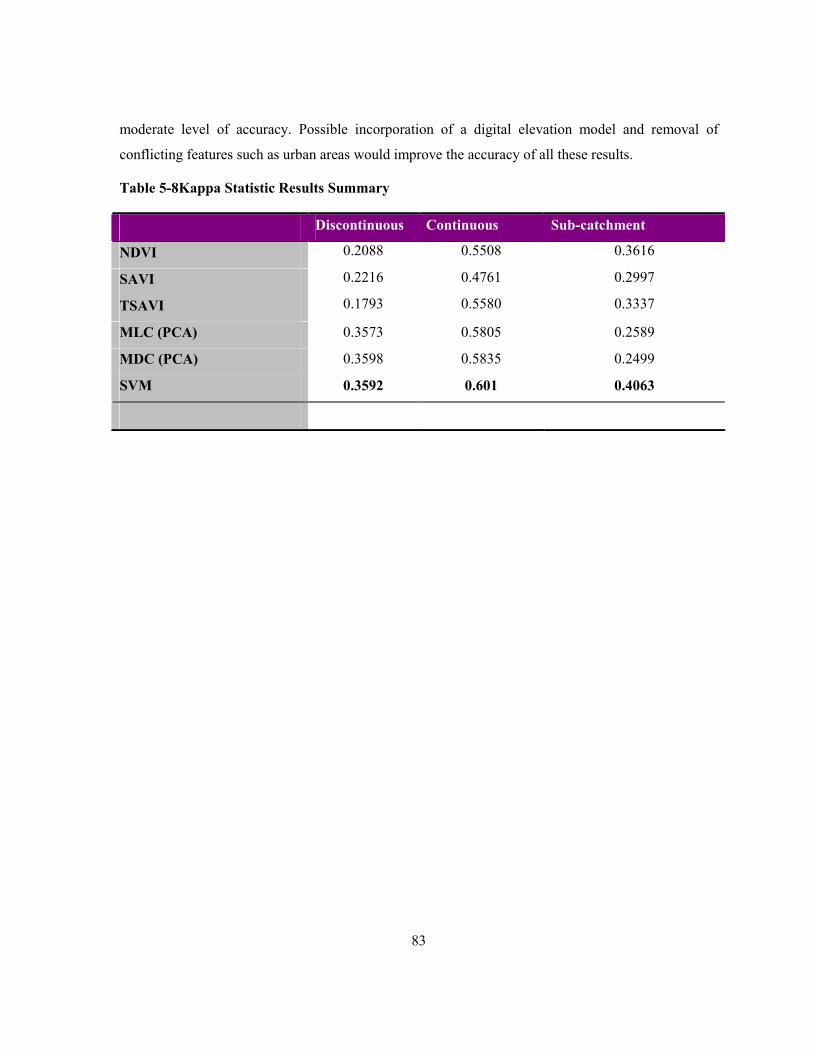
83
moderate level of accuracy. Possible incorporation of a digital elevation model and removal of
conflicting features such as urban areas would improve the accuracy of all these results.
Table 5-8Kappa Statistic Results Summary
Discontinuous Continuous Sub-catchment
NDVI 0.2088 0.5508 0.3616
SAVI 0.2216 0.4761 0.2997
TSAVI 0.1793 0.5580 0.3337
MLC (PCA) 0.3573 0.5805 0.2589
MDC (PCA) 0.3598 0.5835 0.2499
SVM 0.3592 0.601 0.4063
84
Chapter 6
Discussion
6.1 Issue of Detectability
Some of the low accuracy results achieved using the proposed semi-automatic techniques can be
explained in terms of detectability - described as the degree of ease or difficulty that is encountered in
extracting a gully using a vegetation index or classification algorithm. The low results for mapping
discontinuous gullies are an issue of detectability both spatially and spectrally. Spatially the issue
relates to the size of discontinuous gullies, which in some cases tends to be less than the pixel size
30*30m². This means that the gully is imbedded in a spectrally mixed pixel that contains components
of non gully areas. Therefore spectral detectability of gullies in a landscape becomes more difficult,
and accuracy in mapping the gully decreases, as the complexity of the background increases (Adams
and Gillespie, 2006). The continuous gully subset produced the highest kappa statistic because the
continuous gully system is a very prominent feature in the landscape, with most of the pixels being
bare soil whereas the discontinuous gully pixels are a mix of vegetation and bare soil. The issue of
detectability also explains the low accuracy results at the sub-catchment subset. First it contains a
mixture of continuous and discontinuous gullies with the latter probably decreasing the accuracy
levels. Second the sub-catchment subset includes a wider range of spectrally similar features to
gullies, such as built up areas and quarries. Figure 6-1 is a TSAVI gully map and the ground truth
gully map illustrating some of the features that were commonly miss-classified as gullies (errors of
commission).

85
Roads
Extraction Site
TSAVI Gully Map Ground truth Gully Map
Figure 6-1 Right: Spectrally similar features that were mapped as gullies. Left: TSAVI gully
map and right is the ground truth gully map
Despite the superior performance of some of the proposed semi-automatic gully mapping techniques
at the continuous gully level, several parts and entire gullies remain unmapped at the sub-catchment
level. Most of the proposed mapping techniques were unable to identify gullies along the escarpment
(error of omission). A possible explanation could be the inclusion of some vegetation within the
gullies which can be seen as a slight pink colour within the expert digitized gully outline in white
colour in Figure 6-2 D. This is an issue of up-scaling, i.e. the application of methods to a larger area.
It is also possible that this error occurred due to elevation distortions because these gullies are located
on a slightly steeper slope than those chosen in the experiments. This steeper slope could have caused
elevation distortions in the VIs; additionally this area could have a perched water table causing the
exposed soil to be on the darker section of the soil line. Thus affecting the proposed soil line VIs and
classification algorithms because these techniques were modeled to the continuous gully subset. A
possible way to overcome this situation would be to apply geographical stratification, based on
elevation. This can be done by using a digital elevation model to observe whether the spectral
response of gullies changes with elevation.

86
Figure 6-2 The location where gullies were not identified using NDVI (A), SAVI (B) and TSAVI
(C); false colour composite (D) with red indicating vegetation and light blue indicating bare
soil; the purple and light blue areas in A, B and C are the errors of omission and commission.
6.2 Possible Explanations for Low Accuracy of Maps
The low accuracy levels obtained overall could also be explained because of the methods used in the
accuracy assessment. First, this case study is unique to most remote sensing accuracy assessments
because it has considered all the pixels in the study region as a sample size since it is a representative
of the entire mapping domain. However, in the real world such as situation may not be possible as it
is time consuming and costly to obtain information about every pixel (digitization). In areas where
there is little known about the erosion status or expert knowledge is unavailable, a sample of pixels

87
can be used to estimate the classification accuracy. However it is important that the map user is
cautions on the decisions made based on these maps because the higher accuracy levels can be very
misleading especially when the area being mapped is only a small percentage of the map. For
example a random sample of 100 non gully points and 75 gully points was generated to test the
accuracy of the SVM sub-catchment map. Using the ground truth image accuracy assessment
discussed in the study, the SVM map had an accuracy of 0.4063, but using the ground truth points the
accuracy increased to 0.55 with an overall accuracy of 80%, which are both misleadingly high results.
Second, the low accuracy could be explained by the temporal resolutions of the imagery used in the
study. The SPOT 5 image used to digitize gullies was taken in 2006 whereas the Landsat TM used to
create the semi-automatic maps was taken in 2005. The major issue is the assumption that a gully
system had not changeover a one year period. As presented in section 2.1.1.3 gully erosion rates can
vary. In one year changes such as flashfloods, human induced factors, vegetation growth and removal
could have caused drastic changes in the landscape and thus gully system. This highlights the
importance of additional information on past events that may have occurred prior to the image
capture. Third the confidence put into the ground truth gully map could cause some discrepancies. As
mentioned earlier there are difficulties in the literature with the characterization of a gully and thus it
can also be expected that the experts digitizing the gully made errors. These are all possible
explanations for the results obtained and can only be justified with further investigation.

88
Chapter 7
Conclusions and Recommendations
As presented in this thesis traditional techniques for mapping gullies were inappropriate for regional
erosion control in South Africa because of the limited resources (expert knowledge, time and money).
Furthermore traditional techniques have proven challenging to use because gullies vary in their
characterization, dimension, development and also in their governing factors. The literature review
discussed how satellite remote sensing can overcome some of the limitations of traditional gully
mapping methods. In this section a detailed overview of candidate satellite remote sensing
instruments for erosion mapping was presented and Landsat TM had the greatest potential for gully
mapping in South Africa. Landsat TM was then combined with selected semi-automatic techniques
for mapping gully erosion in Kwazulu-Natal South Africa.
The complex nature of gully erosion and its surrounding areas also proved to be challenging for gully
mapping using some of the explored vegetation indices and conventional classifiers. The
heterogeneity of the gullies themselves limited the mapping capabilities of the vegetation indices
because the thresholds masked the area based on vegetated and non vegetated, not necessarily gully
and no gully. The application of the conventional classification algorithms, MLC and MDC, were not
appropriate for mapping gullies in this case study because they assume implicitly that the set of
classes were exhaustively defined which was not the case because only two classes were being used
to map the area, gully and non-gully area. However, SVM proved to be superior over all the explored
methods and is recommended for future gully erosion mapping studies in South Africa because it:
• Required less expert knowledge in the training stages:
o SVM produced a moderate accuracy level by successfully separating the gully class
from the non gully class using a small training data set.
• Required less time:
o In processing because no image transformation was necessary
o In training data collection, small training data size.
• The achieved accuracies were comparable to traditional gully mapping methods.
89
• Once the parameters were defined the algorithm was simple to run.
SVM can be beneficial for erosion control, not only in South Africa, but other regions around the
world. The potential of using SVM to map areas of severe erosion provides a means of obtaining
valuable information on the extent, nature and magnitude of gully erosion in remote areas. This study
has demonstrated that SVM can be used for the spatial assessment of the driving forces present at
different scales- defined as subcatchment, continuous and discontinuous, which is considered to be
relevant in future steps towards controlling erosion in South Africa (Sonneveld et al., 2005).
Stakeholders in erosion management can have added benefit of knowing the accuracy of the maps
produced and thus make better decisions quickly because the technique is repeatable. The technique is
also affordable and requires less expert knowledge. However users must be aware about the scale
(discontinuous, continuous or sub-catchment) at which they require the gully maps because as
demonstrated in this thesis higher accuracies are more achievable when the gully erosion feature is
more prominent, as in the continuous gully scale. The overall accuracies achieved were low because
of the methods used in the accuracy assessment and also possible because of the temporal resolution
of the imagery. For improved accuracy in gully mapping for future studies the following is
recommended:
• Higher spatial and spectral resolution imagery. This would be necessary to for a more
accurate local gully erosion map 1:10,000 (Thwaites, 1986).
• Incorporation of ancillary information: e.g. elevation, slope, and aspect could improve the
understanding of how the terrain affects the radiation of features. For example with the SVM,
information on soil moisture levels and other properties could help in the training data
acquisition process in order to identify the most informative training samples (Mathur and
Foody, 2008).
• Combining SPOT and Landsat TM imagery: could provide a higher accuracy for mapping
gullies because the classifiers would have the advantage of having both a high spatial
resolution from SPOT and a high spectral resolution from the Landsat TM.
• Mask out spectrally similar features such as, urban built up areas, prior to mapping the gullies
with the proposed techniques.
• Use ground truth imagery with the same temporal resolution.

90
• Design and explore other indices for mapping gullies because there are currently none that
are specific to geomorphic features that contain vegetation and bare soil.
91
References
Adams, J. B., and Gillespie, A. R. (2006). Remote sensing of landscapes with spectral images: A
physical modeling approach. Cambridge: Cambridge University Press.
ARC. (2007). Agricultural research council: Spatial data. Unpublished manuscript.
Atkinson, P. M., and Tate, J. N. (Eds.). (1999). Advances in remote sensing and GIS analysis. West
Sussex, England: John Wiley and Sons Ltd.
Bader, C. J. (Ed.). (1962). Typical soils of the east London district. the border region, natural
environment and land use in the eastern cape. Cape Town: Oxford University Press.
Baret, F., and Guyot, G. (1991). Potentials and limits of vegetation indices for LAI and APAR
assessment. Remote Sensing of Environment, 35(2-3), 161-173.
Baret, F., Jacquemoud, S., and Hanocq, J. F. (1993). The soil line concept in remote sensing. Remote
Sensing Reviews, 7(1), 65-82.
Bergsma, E. (1974). Soil erosion sequences on aerial photographs. The ITC Journal, (3), 342-376.
Barnes, E. M., and Baker, M. G. (2000). Multispectral data for mapping soil texture: Possibilities and
limitations. Application of Engineering and Agriculture, 16, 731-741.
Baugh, W. M., and Groeneveld, D. P. (2006). Broadband vegetation index performance evaluated for
a low-cover environment. International Journal of Remote Sensing, 27(21), 4715.
Beckedahl, H., and Dardis, G. F. (1988). The role of artificial drainage in the development of soil
pipes and gullies: Some examples from Transkei, southern Africa. In G. F. Dardis, and B. P.
Moon (Eds.), Geomorphological studies in southern Africa, (pp. 229-245). Rotterdam,
Netherlands: Balkema.
Bergsma, E. (1974). Soil erosion sequences on aerial photographs. The ITC Journal, (3), 342-376.
Berjak, M., Fincham, R., Liggitt, B. and Watson, H. (1986). Temporal and spatial dimensions of gully
erosion in northern natal, south Africa. Commission IV of the International Society for
Photogrammetry and Remote Sensing and the Remote Sensing Society, Pollock Halls,
Edinburgh, Scotland.

92
Blong, R. J. (1966). Discontinuous gullies on the volcanic plateau. New Zealand Journal of
Hydrology, 5, 87-99.
Boardman, J. (2006). Soil erosion science: Reflections on the limitations of current approaches.
Catena, 68(2-3), 73-86.
Bocco, G. (1991). Gully erosion: Processes and models. Progress in Physical Geography, 15(4), 392-
406.
Bocco, G., Palacio, J. L. and Valenzuela, C. R. (1991). Gully erosion modeling using GIS and
geomorphological knowledge. ITC Journal, 3, 253-261.
Bocco, G. and Valenzuela, C. R. (1988). Integration of GIS and image processing in soil erosion
studies using ILWIS. ITC Journal, 4, 309-319.
Bocco, G. and Valenzuela, C. R. (1993). Integrating satellite-remote sensing and geographic
information systems technologies in gully erosion research. Remote Sensing Reviews, 7(3-4),
233-240.
Botha, G. A. (1996). The geology and palaeopedology of late quaternary colluvial sediments in
northern KwaZulu-natal. Council for Geoscience, South Africa, Memoir 83, 165.
Botha, J. H., and Fouche, P. S. (2000). An assessment of land degradation in the northern province
from satellite remote sensing and community perception. South African Geographical Society,
82, 70-79.
Botha, G. A., Wintle, A. G. and Vogel, J. C. (1994). Episodic late quaternary palaeogully erosion in
northern KwaZulu-natal, South Africa. Catena, 23, 327-340.
Boyd, D., Sanchez-Hernandez, C., and Foody, G. M. (2006). Mapping a specific class of interest for
priority habitats monitoring from satellite sensor data. International Journal of Remote Sensing,
27(13), 2631-2644.
Brill, J., and Ochs, B. (2008). NASA: Landsat data continuity mission. Retrieved November, 01,
2008, from http://ldcm.nasa.gov/
Bull, L. J. and Kirkby, M. J. (1997). Gully processes and modeling. Progress in Physical Geography,
(21), 354-374.
Burges, C. J. C. (1998). A tutorial on support vector machines for pattern recognition. Data Mining
and Knowledge Discovery, 2, 121-167.
93
Burkard, M. B. and Kostaschuk, R. A. (1997). Patterns and controls of gully growth along the
shoreline of lake Huron. Earth Surface Processes and Landforms, 22, 901-911.
Camps-Valls, G., Gomez-Chova, L., Calpe-Maravilla, J., Martin-Guerrero, J. D., Soria-Olivas, E.,
Alonso-Chorda, L., et al. (2004). Robust support vector method for hyperspectral data
classification and knowledge discovery
Chalela, Q., Stocking, M. (1988). An improved methodology for erosion hazard mapping: PartII.
application to Lesotho. Geographiska Annaler, 10A(3), 181-189.
Charlton, R. (2008). Fundamentals of fluvial geomorphology. New York: Routedge, Taylor and
Fancis Group.
Cihlar, J., Latifovic, R., Beaubien, J., Guindon, B., and Palmer, M. (2003). TM-based accuracy
assessment of a land cover produce for Canada derived from SPOT VEGETATION data.
Canadian Journal of Remote Sensing, 29(2), 154-170.
Congalton, R. G. (1991). A review of assessing the accuracy of classifications of remotely sensed
data. Remote Sensing of Environment, 37(1), 35-46.
Cogalton, R. G., and Green, K. (1999). Assessing the accuracy of remote sensed data: Principles and
practices. London New York: Lewis Publishers.
Cyr, L., Bonn, F., and Pesant, A. (1995). Vegetation indices derived from remote sensing for an
estimation of soil protection against water erosion. Ecological Modeling, 79(1-3), 277-285.
Dang, A., Zhang, S., He, X., Tang, L., & Xu, H. (2003). Case study on soil erosion supported by GIS
and RS
Dardis, G. F. (1991). The role of rock properties in the development of bedrock-incision rills and
gullies: Examples from South Africa. GeoJournal, 23(1), 35-40.
Dardis, G. F., Beckedahl, H., Bowyer-Bower, T. A. S. and Hanvey, P. M. (1988). Soil erosion forms
in southern Africa. In G. F. Dardis and B. P. Moon (Eds.), Geomorphological studies in southern
Africa (pp. 187-213). Rotterdam, Netherlands: Balkema.
Dash, J., Mathur, A., Foody, G. M., Curran, P. J., Chipman, J. W., and Lillesand, T. M. (2007). Land
cover classification using multi-temporal MERIS vegetation indices. International Journal of
Remote Sensing, 28(6), 1137.
de Asis, A. M., and Omasa, K. (2007). Estimation of vegetation parameter for modeling soil erosion
using linear spectral mixture analysis of Landsat ETM data. ISPRS Journal of Photogrammetry
and Remote Sensing, 62(4), 309-324.

94
de Jong, S. M. (1994). Applications of reflective remote sensing for land degradation studies in a
Mediterranean environment. University Utrecht: Netherlands: Faculteit Ruimtelijke
Wetenschappen.
Dhakal, A. S., Amada, T., Aniya, M., and Sharma, R. R. (2002). Detection of areas associated with
flood and erosion caused by a heavy rainfall using multitemporal landsat TM data.
Photogrammetric Engineering and Remote Sensing, 68(3), 233-239.
DWAF. (2007). Geospatial data. Pretoria: Department of Water Affairs and Forestry.
Dwivedi, R. S., Kumar, A. B., and Tewari, K. N. (1997). The utility of multi-sensor data for mapping
eroded lands. International Journal of Remote Sensing, 18(11), 2303-2318.
Dwivedi, R. S., and Ramana, K. V. (2003). The delineation of reclamative groups of ravines in the
indo-gangetic alluvial plains using IRS-ID LISS-III data. International Journal of Remote
Sensing, 24(22), 4347-4355.
Dwivedi, R. S., RaviSankar, T., Venkataratnam, L., Karale, R. L., Gawande, S. P., SeshagiriRao, K.
V., et al. (1997). The inventory and monitoring of eroded lands using remote sensing data.
International Journal of Remote Sensing, 18(1), 107-119.
Ellis, F. (2000). The application of machine learning techniques to erosion modeling. Unpublished
manuscript.
Eswaran, H., Lal, R. and Reich, P. F. (2001). Land degradation: An overview. Response to Land
Degradation , 20-35.
Fadul, H. M., Salih, A. A., Imad-eldin, A. A. and Inanaga, S. (1999). Use of remote sensing to map
gully erosion along the Atbara River, Sudan. International Journal of Applied Earth Observation
and Geoinformation, 1(3-4), 175-180.
Felix-Henningsen, P., Morgan, R. P. C., Mushala, H. M., Rickson, R. J. and Scholten, T. (1997). Soil
erosion in Swaziland: A synthesis. Soil Technology, 11(3), 319-329.
Flugel, W., Marker, M., Moretti, S., Rodolfi, G. and Sidorchuk, A. (2003). Integrating geographical
information systems, remote sensing, ground truthing and modeling approaches for regional
erosion classification of semi-arid catchments in South Africa. Hydrological Processes, 17(5),
929-942.
Food and Agriculture Organization (FAO). (1965). Soil erosion by water. some measures for its
control on cultivated lands. No. 81). Rome: FAO Agricultural Paper.

95
Foody, G. M., and Arora, M. K. (1997). An evaluation of some factors affecting the accuracy of
classification by an artificial neural network. International Journal of Remote Sensing, 18, 799-
810.
Foody, G. M., and Mathur, A. (2004a). A relative evaluation of multiclass image classification by
support vector machines. IEEE Transactions on Geoscience and Remote Sensing, 93, 1335-
1343.
Foody, G. M., and Mathur, A. (2004b). Toward intelligent training of supervised image
classifications: Directing training data acquisition from SVM classification. Remote Sensing of
Environment, 93, 107-117.
Foody, G. M., and Mathur, A. (2006). The use of small training sets containing mixed pixels for
accurate hard image classification: Training on mixed spectral responses for classification by a
SVM. Remote Sensing of Environment, 103(2), 179-189.
Foody, G. M., Mathur, A., Sanchez-Hernandez, C., and Boyd, D. S. (2006). Training set size
requirements for the classification of a specific class. Remote Sensing of Environment, 104(1), 1-
14.
Fox, G. A., Sabbagh, G. J., Searcy, S. W., and Yang, C. (2004). An automated soil line identification
routine for remotely sensed images. Soil Science Society of America, 68, 1326-1331.
Fox, R. C. and Rowntree, K. M. (Eds.). (2001). Redistribution and reform: Prospects for the land in
the eastern cape province, South Africa. Kluwer Academic Publishers: Dordrecht.
Garland, G. G., Hoffman, T. and Todd, S. (2000). Soil degradation in a national review of land
degradation in South Africa. Retrieved 06/01, 2008, from
Gilabert, M. A., González-Piqueras, J., García-Haro, F. J., and Meliá, J. (2002). A generalized soil-
adjusted vegetation index. Remote Sensing of Environment, 82(2-3), 303-310.
Giordano, A., and Marchisio, C. (1991). Analysis and correlation of the existing soil erosion maps in
the Mediterranean basin. Quaderni Di Scieza Del Suolo, 3, 97-132.
Gualtieri, J. A., Chettri, S. R., Cromp, R. F., and Johnson, L. F. (1999). Support vector machine
classifiers as applied to AVIRIS data. Unpublished manuscript.
Hadley, R. F., Lal, R., Onstad, C. A., Walling, D. E. and Yair, A. (1985). Recent developments in
erosion and sediment yield studies. Technical Documents in Hydrology,
Harvey, M. D., Watson, C. C. and Schumm, S. A. (1985). Gully erosion. Technical Note, (366)

96
Hayden, R. S. (2008). NASA geomorphology: Mapping. Retrieved October/10, 2008, from
http://disc8.sci.gsfc.nasa.gov/geomorphology/GEO_11
Heede, B. H. (1970). Morphology of gullies in the Colorado rocky mountains. Bulletin International
Association of Science and Hydrology, XV(2), 78-89.
Heede, B. H. (1975). Stages of development of gullies in the west No. ARS-S-40). Washington: US
Department of Agriculture.
Hermes, L., Frieauff, D., Puzicha, J., and Buhmann, J. M. (1999). Support vector machines for land
usage classification in Landsat TM imagery. Hamburg, Germany. 348-350.
Hill, J., and Schutt, B. (2000). Mapping complex patterns of erosion and stability in dry
Mediterranean ecosystems. Remote Sensing of Environment, 74(3), 557-569.
Hoffer, R. M., & Johannsen, C. J. (1969). Ecological potentials in spectral signature analysis. In P. L.
Johnson (Ed.), (pp. 1-29). Athens: University of Georgia Press.
Hoffman, T. and Ashwell, A. (2001). Nature divided land degradation in South Africa. Cape Town:
University of Cape Town Press.
Hsu, C., Chang, C., and Lin, C. -. (2008, ). A practical guide to support vector classification.
Huang, C., Davis, L. S., and Townshend, J. R. G. (2002). An assessment of support vector machines
for land cover classification. International Journal of Remote Sensing, 23(4), 725-749.
Huete, A. R. (1988). A soil-adjusted vegetation index (SAVI). Remote Sensing of Environment, 25(3),
295-309.
Huete, A. R., Hua, G., Qi, J., Chehbouni, A., and van Leeuwen, W. J. D. (1992). Normalization of
multidirectional red and NIR reflectance’s with the SAVI. Remote Sensing of Environment,
41(2-3), 143-154.
Hudson, N. W. (1980). Erosion prediction with insufficient data. In M. D. E. Boodt and D. Gabriels
(Eds.), Assessment of erosion (pp. 279). Great Britain: John Wiley and sons.
Imeson, A. C. and Kwaad, F. J. (1980). Gully types and gully prediction. Geografisch Tijdschrift,
XIV(5), 430-41.
Ireland, H. A., Sharpe, C. F. and Eargle, D. H. (1939). Principles of gully erosion in the piedmont of
South Carolina. Technical Bulletin, (633)

97
Irons, J. R., Weismiller, R. A., and Petersen, G. W. (1989). Soil reflectance. In G. E. Asrar (Ed.),
Theory and applications of optical remote sensing (pp. 66). New York: Wiley.
Jackson, R. D. (1983). Spectral indices in N-space. Remote Sensing of Environment, 13(5), 409-421.
Jackson, R. D., and Huete, A. R. (1991). Interpreting vegetation indices. Preventive Veterinary
Medicine, (11), 185-200.
Jensen, J. R. (2005). Introductory digital image processing (3rd ed.). United States of America:
Pearson Prentice Hall.
Joachims, T. (1998). Text categorization with support vector machines learning with many relevant
features. Berlin. 137-142.
Jones, R. G. B. and Keech, M. A. (1966). Identifying and assessing problem areas in soil erosion
surveys using aerial photographs. Photogrammetric Society, 5(27), 189-197.
Jurgens, C., and Fander, M. (1993). Soil erosion assessment and simulation by means of SGEOS and
ancillary digital data. International Journal of Remote Sensing, 14(15), 2847-2855.
Kakembo, V. and Rowntree, K. M. (2003). The relationship between land use and soil erosion in the
communal lands near peddie town, eastern cape, South Africa. Land Degradation and
Development, 14, 39-49.
King, R. B. (2002). Land cover mapping principles: A return to interpretation fundamentals.
International Journal of Remote Sensing, 23(18), 3525-3545.
King, C., Baghdadi, N., Lecomte, V., and Cerdan, O. (2005). The application of remote-sensing data
to monitoring and modeling of soil erosion. Catena, 62(2-3), 79-93.
Kiusi, R. B. and Meadows, M. E. (2006). Assessing land degradation in the monduli district, northern
Tanzania. Land Degradation and Development, 17, 509-525.
Klimaszewski, M. (1982). Detailed geomorphological maps. ITC Journal, 3, 265-271.
Lai, C., Tax, D. M. J., Duin, R. P. W., Pekalska, E., and Paclik, P. (Eds.). (2002). On combining one-
class classifiers for image database retrieval. Berlin Heidelberg: Springer-Verlag.
Lafarge, F., Descombes, X., and Zerubia, J. (2005). Textural kernel for SVM classification in remote
sensing: Application to forest fire detection and urban area extraction. IEE,

98
Laker, M. C. (2000). Soil resources: Distribution, utilization and degradation. In R. Fox and K.
Rowntree (Eds.), The geography of South Africa in a changing world (pp. 326). Cape Town:
Oxford University Press Southern Africa.
Lal, R. (2001). Soil degradation by erosion. Land Degradation and Development, 12(6), 519-539.
Langran, K. J. (1983). Potential for monitoring soil erosion features and soil erosion modeling
components from remotely sensed data. Proc. IGARSS 83,
Lawrence, R. L., and Ripple, W. J. (1998). Comparisons among vegetation indices and band wise
regression in a highly disturbed, heterogeneous landscape: Mount St. Helens, Washington.
Remote Sensing of Environment, 64(1), 91-102.
Le Roux, J. J., Newby, T. S. and Summer, P. D. (2007). Monitoring soil erosion in South Africa at a
regional scale: Review and recommendations. South African Journal of Science, 103, 329-335.
Leopold, L. B. and Miller, J. P. (1956). Ephemeral streams, hydraulic factors and their relation to the
drainage net. US Geological Survey, 282-A
Leopold, L. B., Wolman, G. M. and Miller, J. P. (1964). Fluvial processes in geomorphology. United
States of America: W.H. Freeman and Company.
Liggitt, B. (1988). An investigation into soil erosion in the Mfolozi catchment. Unpublished
manuscript.
Liggitt, B. and Fincham, R. J. (1989). Gully erosion: The neglected dimension in soil erosion
research. South African Journal of Science, 85, 18-20.
Lu, D., and Weng, Q. (2007). A survey of image classification methods and techniques for improving
classification performance. International Journal of Remote Sensing, 28(5), 823-870.
Lawrence, R. L., and Ripple, W. J. (1998). Comparisons among vegetation indices and band wise
regression in a highly disturbed, heterogeneous landscape: Mount St. Helens, Washington.
Remote Sensing of Environment, 64(1), 91-102.
Mantero, P., and Moser, G. (2005). Partially supervised classification of remote sensing images
through SVM-based probability density estimation. IEEE Transactions on Geoscience and
Remote Sensing, 43(3), 559-570.
Mather, P. M. (2004). Computer processing of remotely-sensed images (Third ed.). England: John
Wiley and Sons Ltd.
99
Mathieu, R., King, C., and Le Bissonnais, Y. (1997). Contribution of multi-temporal SPOT data to
the mapping of a soil erosion index. the case of the loamy plateau of northern France. Soil
Technology, 10(2), 99-110.
Mathur, A., and Foody, G. M. (2008). Crop classification by support vector machine with
intelligently selected training data for an operational application. International Journal of
Remote Sensing, 29(8), 2227-2240.
Mati, B. M. and Veihe, A. (2008). Application of the USLE in a savannah environment: Comparative
experiences from east and west Africa. Singapore Journal of Tropical Geography, 22(2), 138.
Meadows, M. E., and Hoffman, T. (2003). Land degradation and climate change in South Africa. The
Geographical Journal, 169(7), 168-177.
Melgani, F., and Bruzzone, L. (2004). Classification of hyperspectral remote sensing images with
support vector machines. IEEE Transactions on Geoscience and Remote Sensing, 42, 1778-
1790.
Merrit, W. S., Letcher, R. A., and Jakeman, A. J. (2003). A review of erosion and sediment transport
models. Environmental Modeling and Software, 18(8-9), 761-799.
Metternicht, G. I., and Fermont, A. (1998). Estimating erosion surface features by linear mixture
modeling. Remote Sensing of Environment, 64(3), 254-265.
Metternicht, G. I., and Zinck, J. A. (1998). Evaluating the information content of JERS-1 SAR and
landsat TM data for discrimination of soil erosion features. ISPRS Journal of Photogrammetry
and Remote Sensing, 53(3), 143-153.
Millington, A. C., and Townshend, J. R. G. (1984). Remote sensing applications in African erosion
and sedimentation studies. Challenges in African Hydrology and Water Resources. Proc. Harare
Symposium, 1984, , 373-384.
Mills, A. J., and Fey, M. V. (2003). Declining soil quality in South Africa: Effects of land use on soil
organic matter and surface crusting. South Africa Journal of Science, 99, 429-436.
Moore, T. R. (1979). Rainfall erosivity in east Africa. Geographiska Annaler, 61A, 136-147.
Morgan, R. P. C. (1986). Soil erosion and conservation. Essex: Longman Group.
Morgan, R. P. C., Rickson, R. J., McIntyre, K., Brewer, T. R. and Altshul, H. J. (1997). Soil erosion
survey of the central part of the Swaziland middleveld. Soil Technology, 11, 263-289.

100
Mosley, M. P. (1972). Evolution of a discontinuous gully system. Annals Association of American
Geographer, 62(4), 655-63.
Mountain, E. D. (1952). Geology of the keiskammahoek
Mpumalanga, D. (2002). Mpumalanga province, state of environment report 2001. KwaZulu-Natal:
Mpumalanga Department of Agriculture, Conservation and Environment.
Mucina, L., and Rutherford, C. M. (2006). The vegetation of South Africa, Lesotho’s and Swaziland.
Pretoria: South African National Biodiversity Institute.
Nichol, J. E., Shaker, A., and Wong, M. S. (2006). Application of high-resolution stereo satellite
images to detailed landslide hazard assessment. Geomorphology, 76, 68-75.
Nizeyimana, E., and Petersen, G. W. (1997). Remote sensing applications to soil degradation
assessments. In R. Lal, W. H. Blum, C. Valentine and B. A. Stewart (Eds.), Methods for
assessment of soil degradation (pp. 393). New York: CRC Press LLC.
Pal, M., and Mather, P. M. (2005). Support vector machines for classification in remote sensing.
International Journal of Remote Sensing, 26(5), 1007-1011.
Patton, P. C., & Schumm, S. A. (1975). Gully erosion, NW Colorado: A threshold phenomenon.
Geology, 3(2), 88-99.
Pickup, G., and Chewings, V. H. (1988). Forecasting patterns of soil erosion in arid lands from
landsat MSS data. International Journal of Remote Sensing, 9(1), 69-84.
Pickup, G., and Nelson, D. J. (1984). Use of Landsat radiance parameters to distinguish soil erosion,
stability and deposition in arid central Australia. Remote Sensing of Environment, 16(3), 195-
209.
Poesen, J., Vandekerckhove, L., Nachtergaele, J., Oostwoud, W. D., Verstraeten, G. and van
Wesemael, B. (2002). Gully erosion in Dryland environments. In Bull, L.J. Kirkby, M.J. (Ed.),
Dryland rivers: Hydrology and geomorphology of semi-arid channels (pp. 62- 229). Chichester:
John Wiley and Sons.
Pretorius, D. J. (1995). The development of a soil degradation management support. Unpublished
manuscript.
Pretorius, D. J. and Bezuidenhout, C. J. (1994). Report on the development of a methodology to
determine the nature, rate and extent of soil erosion in South Africa No. GW1A/94/7). Pretoria:
National Department of Agriculture, Directorate Land and Resources Management.
101
Price, K. P. (1993). Detection of soil erosion within pinyon-juniper woodlands using thematic mapper
(TM) data. Remote Sensing of Environment, 45(3), 233-248.
Richards, J. A., and Jia, X. (2006). Remote sensing digital image analysis: An introduction (4th ed.).
Germany: Springer.
Richardson, A. J., and Wiegand, C. L. (1977). Distinguishing vegetation from soil background
information. Photogrammetric Engineering and Remote Sensing, 43(12), 1541-1552.
Ritchie, J. C. (2000). Soil erosion. Remote sensing in hydrology and water management (Schultz GA,
Engman ET ed., pp. 271). Berlin: Springer.
Robinovoe, C. J., Chavez Jr, P. S., and Dale, G. (1981). Arid land monitoring using Landsat albedo
difference images. Remote Sensing of Environment, 11, 133-156.
Roli, F., and Fumera, G. (2001). Support vector machines for remote sensing image classification. ,
4170 160-166.
Sabins, F. F. (1996). Remote sensing: Principles and interpretation (3rd ed.). United States of
America: New York: W.H.Freeman and Company.
Sanchez-Hernandez, C., Boyd, D. S., and Foody, G. M. (2007a). Mapping specific habitats from
remotely sensed imagery: Support vector machine and support vector data description based
classification of coastal saltmarsh habitats. Ecological Informatics, 2(2), 83-88.
Sanchez-Hernandez, C., Boyd, D., and Foody, G. M. (2007b). One-class classification for mapping a
specific land cover class: SVDD classification of fenland. IEEE Transactions on Geoscience and
Remote Sensing, 45(4)
Schulze, R. E., Maharaj, M., Lynch, S. D., Howe, B. J., and Melvil-Thomson, B. (1997). South
African atlas of agrohydrology and climatology (first ed.). Pretoria: Water Research
Commission.
Scotney, D. (1978). Soil erosion in natal. paper presented to the wildlife society of southern Africa
symposium on agriculture and environmental conservation. Unpublished manuscript.
Schowengerdt, R. A. (2007). Remote sensing: Models and methods for image processing (3rd ed.).
United States of America: Elsevier Inc.
Servenay, A., and Prat, C. (2003). Erosion extension of indurated volcanic soils of Mexico by aerial
photographs and remote sensing analysis. Geoderma, 117(3-4), 367-375.
102
Shonk, J. L., Gaultney, L. D., Schulze, D. G., and Van Scoyoc, G. E. (1991). Spectroscopic sensing
of soil organic matter content. ASAE, (34)
Sidorchuk, A. (1999). Dynamic and static models of gully erosion. CATENA, 37(3-4), 401-414.
Singh, D., Herlin, I., Berroir, J. P., Silva, E. F., and Simoes, M. M. (2004). An approach to correlate
NDVI with soil colour for erosion process using NOAA/AVHRR data. Advances in Space
Research, 33(3), 328-332.
Soil Science Society of America. (1996). Glossary of soil science terms. USA: Madison.
Song, C., Woodcock, C. E., Seto, K. C., Lenney, M. P., and Macomber, S. A. (2001). Classification
and change detection using Landsat TM data. Remote Sensing of Environment, 75(2), 230-244.
Sonneveld, M. P. W., Everson, T. M. and Veldkamp, A. (2005). Multi-scale analysis of soil erosion
dynamics in Kwazulu-natal, South Africa. Land Degradation and Development, 16(3), 287-301.
Story, M., and Congalton, R. G. (1986). Accuracy assessment: A user's perspective. Photogrammetric
Engineering and Remote Sensing, (52)
Sujatha, G., Dwivedi, R. S., Sreenivas, K., and Venkataratnam, L. (2000). Mapping and monitoring
of degraded lands in part of jaunpur district of uttar pradesh using temporal spaceborne
multispectral data. International Journal of Remote Sensing, 21(3), 519-531.
Summer, P. D. and Meiklejohn, I. (2000). Landscape evolution in a changing environment. In R. Fox
and K. Rowntree (Eds.), The geography of South Africa in a changing world (). Cape Town:
Oxford University Press Southern Africa.
Symeonakis, E., and Drake, N. (2004). Monitoring desertification and land degradation over sub-
Saharan Africa. International Journal of Remote Sensing, 25(3), 573-592.
Tax, D. M. J., and Duin, R. P. W. (2004). Support vector data description. Machine Learning, 54, 45-
66.
Teng, W. L., Loew, E. R., Ross, D. I., Zsilinszky, V. G., Lo, C. P., Philipson, W. R., et al. (1997).
Fundamentals of photographic interpretation. In W. R. Philipson (Ed.), Manual of photographic
interpretation (pp. 49-113). American Society of Photogrammetry and Remote Sensing:
Bethesda.
Terrence, J., Foster, G. and Renard, G. K. (Eds.). (2002). Soil erosion: Processes, predictions,
measurement and control. New York: John Wiley and Sons.
103
Thiam, A. K. (2003). The causes and spatial pattern of land degradation risk in southern Mauritania
using multitemporal AVHRR-NDVI imagery and field data. Land Degradation and
Development, 14(1), 133-142.
Thwaites, R. N. (1986). A technique for local soil erosion survey. South African Geographical
Journal, 68(1), 67-76.
Twidale, C. R. (2004). River pattern and their meaning. Earth Science Review, 67, 159-218.
Vaidyanathan, N. S., Sharama, G., Sinha, R., and Dikshit, O. (2002). Mapping of erosion intensity in
the Garhwali Himalaya. International Journal of Remote Sensing, 23(20), 4125-4129.
van der Eyck, J.J., MacVicar, C. N. and de Villiers, J. M. (1969). Soils of the Tugela basin - a study in
sub-tropical Africa No. 15) Natal Town and Regional Planning Report.
Van Dijk, A., Bruijnzeel, L. and Rosewell, C. (2002). Rainfall intensity-kinetic energy relationships:
A critical literature appraisal. Journal of Hydrology, 261, 1-23.
Van Zuidam, R. E. (1985). Terrain analysis and classification using aerial photographs (2nd ed.).
Enschede: International Institute for Aerospace Survey and Earth Science.
Vapnik, V. N. (1995). The nature of statistical learning theory. New York: Springer-Verlag.
Vapnik, V. N. (1998). Statistical learning theory. New York: Wiley.
Vrieling, A. (2006). Satellite remote sensing for water erosion assessment: A review. Catena, 65, 2-
18.
Vrieling, A., de Jong, S. M., Sterk, G., and Rodrigues, S. C. (2008). Timing of erosion and satellite
data: A multi-resolution approach to soil erosion risk mapping. International Journal of Applied
Earth Observation and Geoinformation, 10(3), 267-281.
Wang, G., Wente, S., Gertner, G. Z., and Anderson, A. (2002). Improvement in mapping vegetation
cover factor for the universal soil loss equation by geostatistical methods with Landsat thematic
mapper images. International Journal of Remote Sensing, 23(18), 3649-3667.
Watson, H. K. (1997). Geology as an indicator of land capability in the mfolozi area, KwaZulu-natal.
South African Journal of Science, 93, 39-44.
Weaver, A. v. (1988). Factors affecting the spatial variation in soil erosion in Ciskei: An initial
assessment at the macroscale. In G. F. Dardis, and B. P. Moon (Eds.), Geomorphological studies
in southern Africa (pp. 215). Rotterdam, Netherlands: Balkema.

104
Weaver, A. v. (1991). The distribution of soil erosion as a function of slope aspect and parent material
in ciskei, South Africa. South Africa GeoJournal, (23), 29-34.
Wessels, K. J., Prince, S. D., Frost, P. E., and van Zyl, D. (2004). Assessing the effects of human-
induced land degradation in the former homelands of northern South Africa with a 1 km
AVHRR NDVI time-series. Remote Sensing of Environment, 91(1), 47-67.
Wilkie, D. S., and Finn, T. J. (1996). Remote sensing imagery for natural resources monitoring. New
York: Columbia University Press.
Whitmore, G., Meth, D. and Uken, R. (2006). Geological science: Geology of KwaZulu-natal.
Retrieved October, 2008, from http://www.geology.ukzn.ac.za/GEM/kzngeol/kzngeol.htm
Wu, D., and Linders, J. (2000). Comparison of three different methods to select feature for
discriminating forest cover types using SAR imagery. International Journal of Remote Sensing,
21(10), 2089-2099.
Zhang, J. and Goodchild, M. F. (Eds.). (2002). Uncertainty in geographical information. New York:
Taylor and Francis

105
Appendix A
Erosion Controlling Factors
Factor Author Findings/Comments
Soil Weaver (1991) Soils with a high clay content as well as a structured A-
horizon tend to exhibit relatively low degrees of erosion.
Duplex soils with restrictive horizons and shallow soils
with a low permeability exhibit higher levels of erosion.
Watson (1997) Unconsolidated sediments and several of the weaker,
particularly shale formations are susceptible to both
gully and sheet erosion
Berjack et al. (1986) and
Liggit (1988)
Soils underlain by Dwyka Tillite were the worst affected
by gulling.
Colluvial or
Sediments
Garland, (2000); Botha,
(1994); Watson, (1997)
In KwaZulu-Natal most gullies form on transported
colluvial or alluvial sediments.
Climate Moore (1979); Van Dijk
(2002)
Affect soil erosion directly, through precipitation,
temperature, evapotranspiration; indirectly, through the
conditions that influence the soil moisture and vegetation
cover (biomass).
Rainfall, in particular, is a major driving force of many
erosional processes and the amount of soil that is
detached is related to rainfall intensity.
Topography Morgan (1986) Important topographical properties regarding degradation
processes are slope steepness, slope length and slope
shape
De Jong (1994) Erosion normally increases with increasing slope
steepness and slope length because of the increase of
velocity and volume of surface runoff
Liggitt (1988) Gradient less than 10° was a critical slope value, where
gullies occur most frequent in part of KZN.
Weaver (1991) North-facing slopes tend to be more heavily eroded than
south-facing slopes because natural forests tend to
concentrate on the cool, moist south-facing slops, hence
restricting erosion.
Bedrock Botha, (1996) Strong direct relationship between gully erosion and
specific bedrock types
Weaver (1991); Berjak
(1986); Mountain
(1952);Bader 1962
Soil erosion is more severe on soils underlain by dolerite
than on those underlain by sedimentary rocks.
Mountain (1952); Berjak
(1986)
Soils underlain by shale’s and mudstone of the Beaufort
Group were more heavily erodable than those underlain
by dolerite

106
Appendix B
Bioregion and vegetation unit map of the Buffalo river sub-catchment (Spatial data source: (Mucina and Rutherford, 2006))

107
Appendix C
Summary of the Biological Environment
1.0 Grassland Biome:
The topography of this biome is mainly flat to rolling, but also includes mountainous regions and the
escarpment. This biome experiences large temperature differences from winter to summer with high frequency
of frost.
1.1 Mesic Highveld Grassland
1.1.1 Wakkerstrom Montane Grassland (Gm14)
• Short montane grassland found on the plateaus and flat areas, with short forest and thickets
occurring along steep, mainly east facing slops and drainage areas.
• Occurs on shallow soils
1.1.2 Paulpietersburg Moist Grassland (Gm15)
• Underlain by Archaean granite and gneiss
• Vulnerable vegetation unit because of its usefulness for cultivation
1.2 Sub Escarpment Grassland
1.2.1 Low escarpment Moist Grassland (Gs3)
• Found on complex mountain topography and on mudstone or shale
1.2.2 Northern KwaZulu-Natal Moist Grassland (Gs4)
• Geology is similar to Gs3 and is considered vulnerable as more than a quarter has already been
transformed either for cultivation, plantation and urban sprawl or by building dams
1.2.3 Northern KwaZulu-Natal Shrubland (Gs5)
• Widely scattered group of patches embedded within Gs4, Gs6 and Gs7.
• Small dolerite koppies and steeper slopes of ridges with sparse grass cover and scattered
shrubland pockets.
1.2.4 KwaZulu-Natal Highland Thorn Shrubland(Gs6)
• Occurs in both dry valleys and moist upland
** 1.2.5 Income Sandy Grassland (Gs7)
• Landscape includes very flat with generally shallow, poorly drained, sandy soils
• Found on sandstones and shale supporting poorly drained sand soils.
1.2.6 Mooi River Highland (Gs8)
• Soils are derived from sedimentary rock and are generally shallow and poor
2.0 Savanna Biome
It is the most widespread biome in Africa. The temperatures in this biome are slightly higher than the
surrounding grasslands mostly due to the lower elevation.
2.1 Sub-escarpment
• 2.1.1 Thukela Thornveld (Sv2)
• Landscape includes valley slopes and undulating hills
3.0 Other Vegetation Units
3.1 Northern Afrotemperate Forest (FOz2)
• Represents the indigenous forest scattered within the study region
3.2 Eastern Temperate Freshwater Wetland (AZf3)
• Found around stagnant water bodies and is embedded within the grassland
(Table modified from Munica and Rutherford (2006)

108
Appendix D
Ground truth study sites (Photographs were taken in October 2007)

109
Appendix E
Support Vector Parameter Test Results
Kernel Kappa statistic Comments
Linear 0.5735 Long processing time
Polynomial 0.5766
Sigmoid 0.5685
Radial Basis
Function (RBF) 0.5794
C parameter Kappa statistic Comments
0.1 0.3 Visually unimpressive gullies appeared wider than normal
50 0.5933 Reduced accuracy and slow
500 0.6002 Faster processing time
1000 0.601 Faster processing time and improved accuracy
Gamma (γ) Kappa statistic Comments
0 - took too long to process results, computer crashed
0.167 0.601 Default value
0.0039 59.79
5 0.5979
60 0.5888