guidance for pacific lamprey distribution and occupancy sampling€¦ · · 2015-06-08guidance...

Guidance for Pacific Lamprey distribution and occupancy sampling:

For the Lamprey occupancy sampling workshop, Tualatin National Wildlife Refuge, Oregon.

Prepared by : Columbia River Fisheries Program Office, U.S. Fish and Wildlife Service

10/27/2014

This document contains draft guidance for the design of a sampling framework and methods at three spatial scales that are selected to inform conservation strategies and actions throughout the range of Pacific Lamprey in the United States.

Draft Guidance CRFPO 10/27/14 Page 1

Guidance for Pacific Lamprey distribution and occupancy sampling

Sampling Frame for evaluating distribution of Pacific Lamprey

Background for the scale of distribution analyses:

Lamprey are among the most poorly studied groups of fishes on the west coast of the United

States, despite their diversity and presence in many rivers including coastal streams (Moyle et

al. 2009). Behavior during the benthic portion of the life-cycle, small size larvae, and the

patchiness of the fine sedimentary habitat they occupy make traditional fish surveys difficult to

successfully implement. Throughout the range of Pacific Lamprey there is very limited

information on adults returning to rivers to track changes in abundance and distribution. The

distribution of a species is a fundamental component of its ability to persist over ecological and

evolutionary time scales (Simberloff 1988; Wahlberg et al. 1996, MacKenzie et al. 2005).

Habitat loss and degradation as well as the extinction of local populations are major threats to a

species’ persistence (Groom et al. 2006). A local population can be defined in biological terms

as a reproductive community of individuals that share in a common gene pool (Dobzhansky

1950). The smallest functional unit of biological interest is generally the local population or in

the case of lamprey a 4th level Hydrologic Unit Code (HUC) (or stock, see Ricker 1972). Given the

limited resources directed towards Pacific Lamprey monitoring, efforts have been focused on

estimating occupancy at a particular scale (assessment unit of interest) and how it is used to

inform distribution of lamprey for a watershed or collection of watersheds for a region of

interest (MacKenzie et al. 2005, Dunham et al. 2013, Jolley et al. 2012, Jolley et al. 2013).

After reviewing a number of the documents guiding Pacific Lamprey conservation and

restoration, we believe that future sampling for Pacific Lamprey can be focused on three spatial

scales to assess conservation progress regionally, by watersheds, and for particular

conservation actions. The three recommended scales are: 1) Regional Management Units

(RMUs); 2) 4th level HUC; and 3) finer scale analysis units within each 4th level HUC. The first


two levels would focus on evaluating changes in distribution at those spatial scales. The third

level would help to inform finer scale issues such as effectiveness of restoration actions or

informing our knowledge on detection probabilities for lamprey for the sampling methods

(focusing on electrofishing approach for larval lamprey).

Based on guidance from section III Status and Distribution of Pacific Lamprey of the

Conservation Agreement (CA, USFWS 2012), the first spatial level of evaluation of distribution

would be at the RMUs for the purpose of implementing conservation actions. Under objective 5

of the Conservation Agreement, the parties agreed to identify historic and current distributions

of Pacific Lamprey in each RMU and monitor them to detect changes in distribution and status

as conservation actions are implemented.

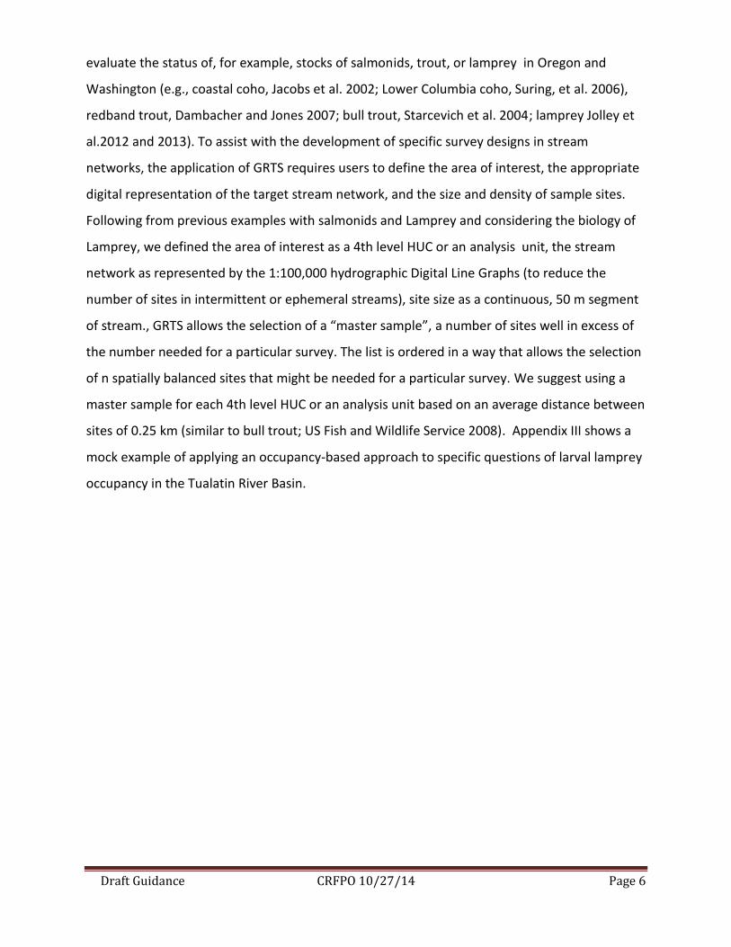
Figure 1 shows the RMUs for Pacific Lamprey in the coterminous United States. Each of these

RMUs includes several 4th level HUCs, which are the geographic units used to evaluate lamprey

status, threats, and watershed specific conservation needs in the Pacific Lamprey Assessment

and Template for Conservation Measures (Luzier et al 2011). Therefore, the first level of

distribution assessment would rely on measuring occupancy of 4th level HUCs of a RMU and to

determine if the occupancy of these HUCs, and therefore the RMU, changed between

assessment periods. The occupancy sampling would focus on the wadeable stream portions of

the HUCs that are suitable for spawning and early rearing. In many of these HUCs various levels

of data exist for direct or indirect sampling that has taken place to verify occupancy. Therefore,

the occupancy sampling at the 4th code HUC would be directed at those HUCs where we lack

recent information (less than 10 years old) to inform occupancy and distribution.

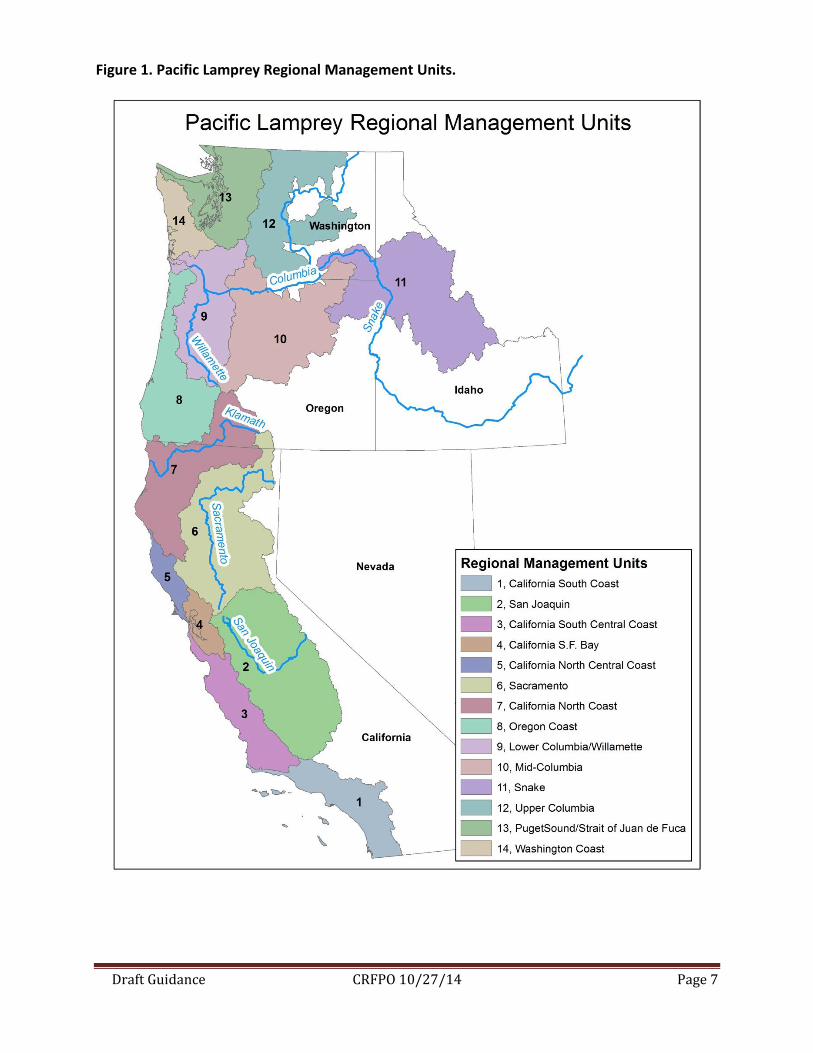
For example, the historic distribution of Pacific Lamprey can be displayed throughout the

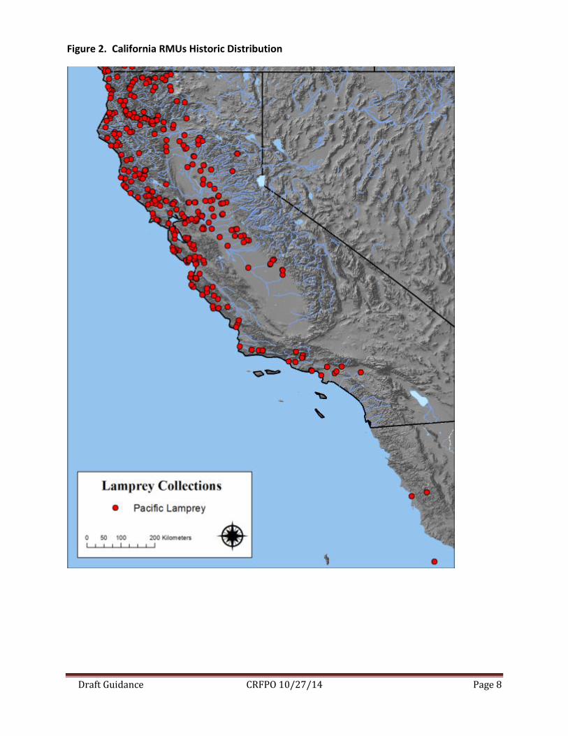
California RMUs (Figure 2). The recent information for stream occupancy of California can be

used to inform distribution changes of the RMUs (Figure 3). However, watersheds that have

unknown occupancy or are determined to be unoccupied (based on sampling for other species

or non-probabilistic sampling) are areas were future probabilistic sampling would be directed to

verify occupancy at the 4th level HUCs (Figure 3 - white circles; Goodman and Reid 2012).


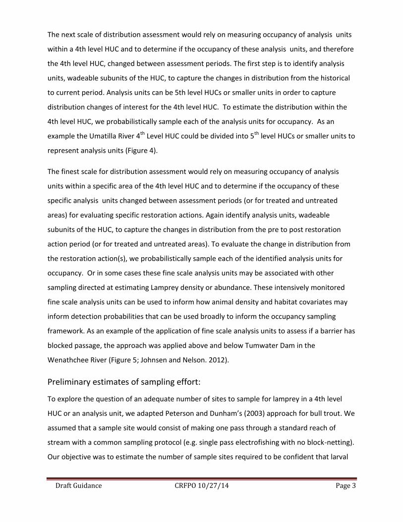
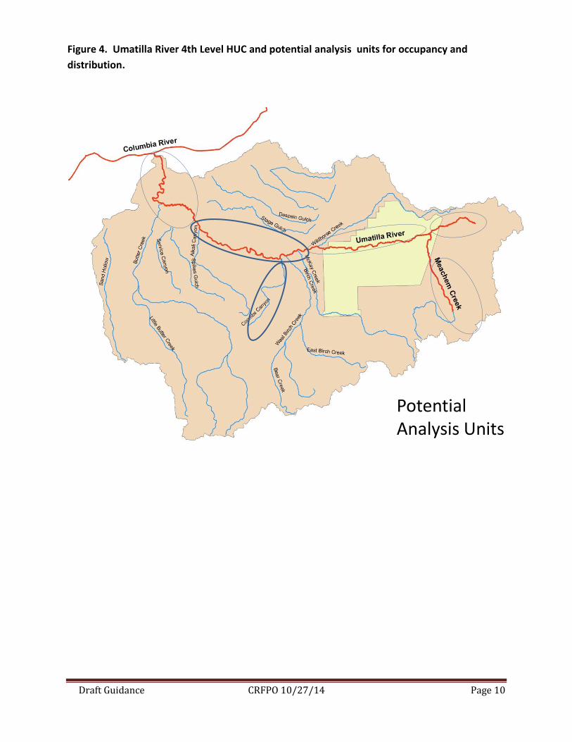
The next scale of distribution assessment would rely on measuring occupancy of analysis units

within a 4th level HUC and to determine if the occupancy of these analysis units, and therefore

the 4th level HUC, changed between assessment periods. The first step is to identify analysis

units, wadeable subunits of the HUC, to capture the changes in distribution from the historical

to current period. Analysis units can be 5th level HUCs or smaller units in order to capture

distribution changes of interest for the 4th level HUC. To estimate the distribution within the

4th level HUC, we probabilistically sample each of the analysis units for occupancy. As an

example the Umatilla River 4th Level HUC could be divided into 5th level HUCs or smaller units to

represent analysis units (Figure 4).

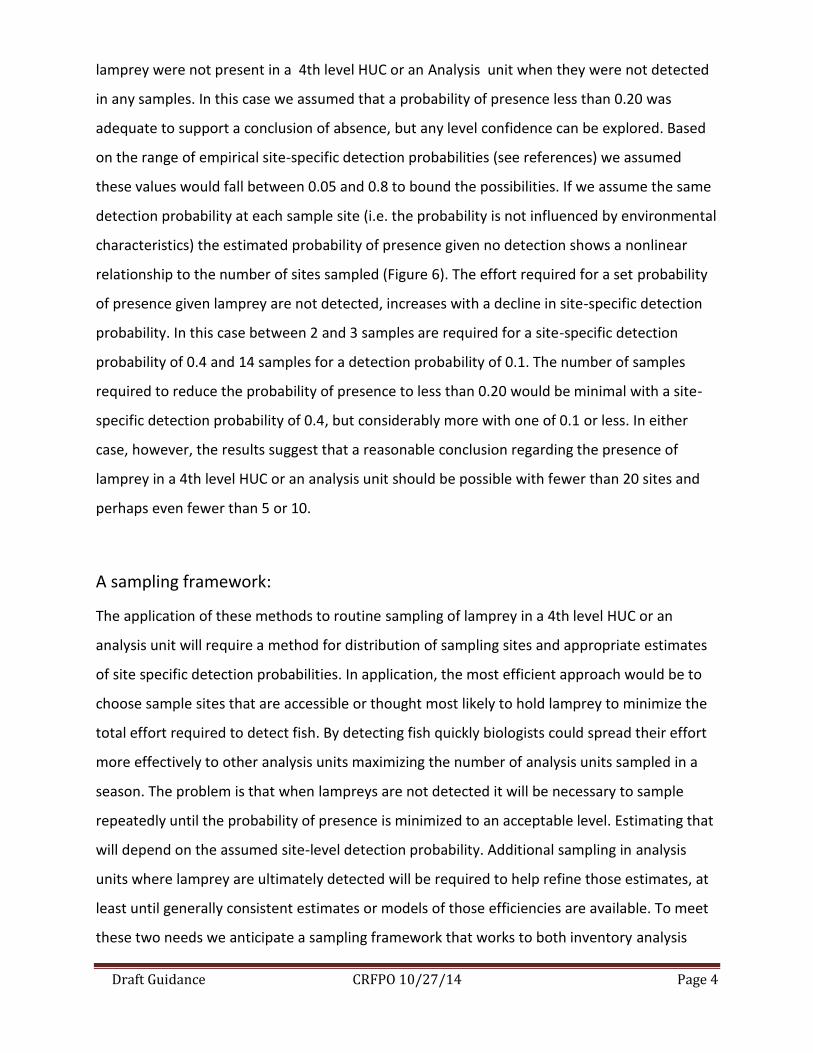
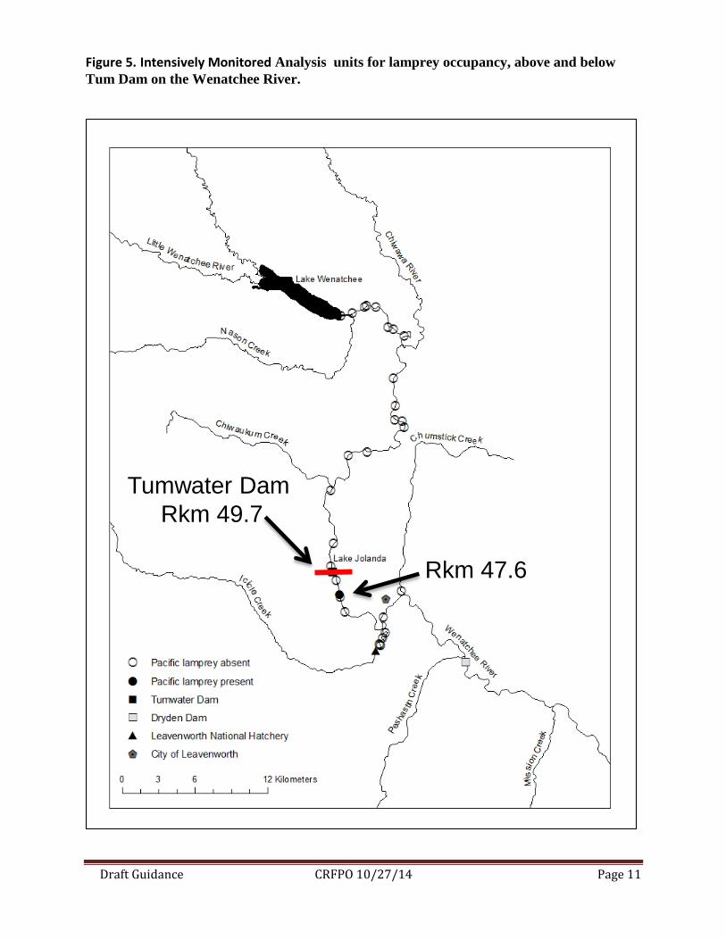
The finest scale for distribution assessment would rely on measuring occupancy of analysis

units within a specific area of the 4th level HUC and to determine if the occupancy of these

specific analysis units changed between assessment periods (or for treated and untreated

areas) for evaluating specific restoration actions. Again identify analysis units, wadeable

subunits of the HUC, to capture the changes in distribution from the pre to post restoration

action period (or for treated and untreated areas). To evaluate the change in distribution from

the restoration action(s), we probabilistically sample each of the identified analysis units for

occupancy. Or in some cases these fine scale analysis units may be associated with other

sampling directed at estimating Lamprey density or abundance. These intensively monitored

fine scale analysis units can be used to inform how animal density and habitat covariates may

inform detection probabilities that can be used broadly to inform the occupancy sampling

framework. As an example of the application of fine scale analysis units to assess if a barrier has

blocked passage, the approach was applied above and below Tumwater Dam in the

Wenathchee River (Figure 5; Johnsen and Nelson. 2012).

Preliminary estimates of sampling effort:

To explore the question of an adequate number of sites to sample for lamprey in a 4th level

HUC or an analysis unit, we adapted Peterson and Dunham’s (2003) approach for bull trout. We

assumed that a sample site would consist of making one pass through a standard reach of

stream with a common sampling protocol (e.g. single pass electrofishing with no block-netting).

Our objective was to estimate the number of sample sites required to be confident that larval


lamprey were not present in a 4th level HUC or an Analysis unit when they were not detected

in any samples. In this case we assumed that a probability of presence less than 0.20 was

adequate to support a conclusion of absence, but any level confidence can be explored. Based

on the range of empirical site-specific detection probabilities (see references) we assumed

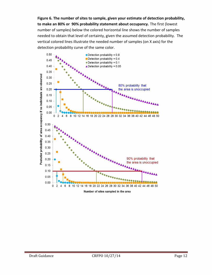
these values would fall between 0.05 and 0.8 to bound the possibilities. If we assume the same

detection probability at each sample site (i.e. the probability is not influenced by environmental

characteristics) the estimated probability of presence given no detection shows a nonlinear

relationship to the number of sites sampled (Figure 6). The effort required for a set probability

of presence given lamprey are not detected, increases with a decline in site-specific detection

probability. In this case between 2 and 3 samples are required for a site-specific detection

probability of 0.4 and 14 samples for a detection probability of 0.1. The number of samples

required to reduce the probability of presence to less than 0.20 would be minimal with a site-

specific detection probability of 0.4, but considerably more with one of 0.1 or less. In either

case, however, the results suggest that a reasonable conclusion regarding the presence of

lamprey in a 4th level HUC or an analysis unit should be possible with fewer than 20 sites and

perhaps even fewer than 5 or 10.

A sampling framework:

The application of these methods to routine sampling of lamprey in a 4th level HUC or an

analysis unit will require a method for distribution of sampling sites and appropriate estimates

of site specific detection probabilities. In application, the most efficient approach would be to

choose sample sites that are accessible or thought most likely to hold lamprey to minimize the

total effort required to detect fish. By detecting fish quickly biologists could spread their effort

more effectively to other analysis units maximizing the number of analysis units sampled in a

season. The problem is that when lampreys are not detected it will be necessary to sample

repeatedly until the probability of presence is minimized to an acceptable level. Estimating that

will depend on the assumed site-level detection probability. Additional sampling in analysis

units where lamprey are ultimately detected will be required to help refine those estimates, at

least until generally consistent estimates or models of those efficiencies are available. To meet

these two needs we anticipate a sampling framework that works to both inventory analysis


units and refine estimates of site specific detection probability simultaneously. If methods are

standardized and results archived in a consistent fashion, the range of observed detection

probabilities and development of detection-covariate models could be shared among

practitioners.

We expect that site-specific detection probabilities will vary with characteristics of the stream

environments that influence sampling efficiency and the distribution and abundance of lamprey

within occupied analysis units (for bull trout: Peterson et al. 2002; Peterson et al. 2004; Thurow

et al. 2006). With enough replicated sampling it could be possible to build empirical models of

site level detection probability that incorporate covariates representing the range of sampling

conditions for lamprey environments and explain that variation. For example, lamprey

occupancy observations are strongly associated with proportion of fine sediment suggesting

that detection probability could improve substantially at areas with high proportion of fines

(type I Habitat-lamprey) within a 4th Level HUC or an analysis unit (J. Great Lakes Res. 29). If

standardized sampling procedures are adopted and sampling results are archived consistently,

the development of new models should be possible allowing the prediction of detection

probabilities based on routine environmental characteristics. Once those models are developed

the need for repeated sampling in any patch for further detection model development will be

lessened. Simulation modeling can illustrate how examining the influence of covariates (e.g.

habitat - type 1 habitat; stream order; density) could be useful to better estimate detection

probability; if such studies are underway (see Appendix II on simulation modeling).

Our goal was to define an initial survey that rigorously estimates analysis unit presence and at

the same time, is practical in the field. The Environmental Protection Agency’s Environmental

Monitoring and Assessment Program (EMAP) developed a general approach for selecting sites

in stream networks incorporating randomization and spatial balance, called GRTS (Generalized

Random- Tessellation Stratified design; Stevens and Olsen 2004). GRTS is a GIS-based approach

and lends itself to a relatively broad application by many users (Firman and Jacobs 2001). GRTS-

based designs allow one to make a statistical inference about the status and trend of stream

attributes (e.g., the presence or absence, or abundance of lamprey) in a predefined stream

network (in this case 4th level HUC or an analysis unit). GRTS has been successfully used to


evaluate the status of, for example, stocks of salmonids, trout, or lamprey in Oregon and

Washington (e.g., coastal coho, Jacobs et al. 2002; Lower Columbia coho, Suring, et al. 2006),

redband trout, Dambacher and Jones 2007; bull trout, Starcevich et al. 2004; lamprey Jolley et

al.2012 and 2013). To assist with the development of specific survey designs in stream

networks, the application of GRTS requires users to define the area of interest, the appropriate

digital representation of the target stream network, and the size and density of sample sites.

Following from previous examples with salmonids and Lamprey and considering the biology of

Lamprey, we defined the area of interest as a 4th level HUC or an analysis unit, the stream

network as represented by the 1:100,000 hydrographic Digital Line Graphs (to reduce the

number of sites in intermittent or ephemeral streams), site size as a continuous, 50 m segment

of stream., GRTS allows the selection of a “master sample”, a number of sites well in excess of

the number needed for a particular survey. The list is ordered in a way that allows the selection

of n spatially balanced sites that might be needed for a particular survey. We suggest using a

master sample for each 4th level HUC or an analysis unit based on an average distance between

sites of 0.25 km (similar to bull trout; US Fish and Wildlife Service 2008). Appendix III shows a

mock example of applying an occupancy-based approach to specific questions of larval lamprey

occupancy in the Tualatin River Basin.


Figure 1. Pacific Lamprey Regional Management Units.


Figure 2. California RMUs Historic Distribution


Figure 3. California RMU Current Distribution


Figure 4. Umatilla River 4th Level HUC and potential analysis units for occupancy and

distribution.

Potential Analysis Units


Figure 5. Intensively Monitored Analysis units for lamprey occupancy, above and below

Tum Dam on the Wenatchee River.

Rkm 47.6

Tumwater Dam

Rkm 49.7


Figure 6. The number of sites to sample, given your estimate of detection probability,

to make an 80% or 90% probability statement about occupancy. The first (lowest

number of samples) below the colored horizontal line shows the number of samples

needed to obtain that level of certainty, given the assumed detection probability. The

vertical colored lines illustrate the needed number of samples (on X axis) for the

detection probability curve of the same color.


References

Dambacher J.M. and K.K. Jones. 2007. Benchmarks and patterns of abundance of redband trout in Oregon streams: a compilation of studies. Pages 47–55 in R.K. Schroeder and J.D. Hall, editors. Redband trout: resilience and challenge in a changing landscape. Oregon Chapter, American Fisheries Society, Corvallis. Dobzhansky, T. 1950. Mendelian populations and their evolution. Amer. Nat. 84:401-418. Dunham, J.B., N.D. Chelgren , M.P. Heck & S.M. Clark 2013. Comparison of electrofishing techniques to detect larval lampreys in wadeable streams in the Pacific Northwest. North American Journal of Fisheries Management, 33:6, 1149-1155, DOI:10.1080/02755947.2013.826758

Firman, J., and S. Jacobs. 2001. A survey design for integrated monitoring of salmonids. Pages 242-252 in T. Nishida, P. J. Kailola, and C. E. Hollingworth, editors. Proceedings of the First International Symposium on Geographic Information Systems (GIS) in Fishery Science. Fishery GIS Research Group, Seattle, Washington. Goodman, D.H. and S.B. Reid. 2012. Pacific lamprey (Entosphenus tridentatus) Assessment and Template for Conservation Measures in California.U.S. Fish and Wildlife Service, Arcata, California. 117 pp. http://www.fws.gov/arcata/fisheries/reports/technical/PLCI_CA_Assessment_Final.pdf Groom M.J., Meffe G.K. and C.R. Carroll. 2006 – Principles of Conservation Biology. Sinauer & Associates, 699 p. Jacobs, S., J. Firman, G. Susac, D. Stewart and J. Weybright. 2002. Status of Oregon Coastal Stocks of Anadromous Salmonids, 2000-2001 and 2001- 2002. Oregon Department of Fish and Wildlife, OPSW-ODFW-2002-3, Portland, Oregon. Jolley J.C., G.S. Silver, and T.A. Whitesel. 2012. Occupancy and detection of larval Pacific Lampreys and Lampetra spp. in a large river: the Lower Willamette River. Transactions of the American Fisheries Society, 141:2, 305-312. Jolley, J.C., G.S. Silver, and T.A. Whitesel. 2013. Occurrence, detection, and habitat use of larval lamprey in Columbia River mainstem Environments: The Dalles Pool and Deschutes River Mouth. U.S. Fish and Wildlife Service, Columbia River Fisheries Program Office, Vancouver, WA. 21 pp. http://www.fws.gov/columbiariver/publications.html Johnsen, A. and M. C. Nelson. 2012. Surveys of Pacific lamprey distribution in the Wenatchee River watershed 2010-2011. U.S. Fish and Wildlife Service, Leavenworth, Washington. http://www.fws.gov/midcolumbiariverfro/reports.html#lamprey Journal of Great Lake Research. 2003. Sea Lamprey International Symposium. Volume 29, Supplement 1. International Association for Great Lakes Research. ISSN 0380-1330.

http://www.fws.gov/arcata/fisheries/reports/technical/PLCI_CA_Assessment_Final.pdf

http://www.tandfonline.com/doi/full/10.1080/00028487.2012.662201

http://www.tandfonline.com/doi/full/10.1080/00028487.2012.662201


Luzier, C.W., H.A. Schaller, J.K. Brostrom, C. Cook-Tabor, D.H. Goodman, R.D. Nelle, K. Ostrand and B. Streif. 2011. Pacific Lamprey assessment and template for conservation measures. U.S. Fish and Wildlife Service. Portland, OR. 282 pages. http://www.fws.gov/columbiariver/publications.html MacKenzie, D., J. Nichols, J. Royce, K. Pollock, L. Bailey, and J. Hines. 2005. Occupancy

Estimation and Modeling- Inferring Patterns and Dynamics of Species Occurrence. Elsevier

Publishing.

Moyle, P. B., L.B. Brown, S. D. Chase, and R. M. Quinones. 2009. Status and conservation of

lampreys in California. Pages 279-293 in L. R. Brown, S. D. Chase, M. G. Mesa, R. J. Beamish,

and P. B. Moyle, editors. Biology, management, and conservation of lampreys in North

America. American Fisheries Society, Symposium 72, Bethesda, Maryland.

Peterson, J.T., J. Dunham, P. Howell, R. Thurow and S. Bonar. 2002. Protocol for determining bull trout presence. Report to the Western Division of the American Fisheries Society. Available: www.fisheries.org/wd/committee/bullptrout/protocolFinal-2–02.doc . Peterson, J. and J. Dunham. 2003. Combining Inferences from Models of Capture Efficiency, Detectability, and Suitable Habitat to Classify Landscapes for Conservation of Threatened Bull Trout. Cons. Biol. 17:1070–1077. Peterson, J.T., R.F Thurow and J.W. Guzevich. 2004. An evaluation of multipass electrofishing for estimating the abundance of stream-dwelling salmonids. Transactions of the American Fisheries Society 133:462-475. Ricker, W.E. 1972. Hereditary and environmental factors affecting certain salmonids populations. Pages 27-160 in (R. C. Simon and P. A. Larkin, editors), The Stock Concept in Pacific Salmon. University of British Columbia, Vancouver, British Columbia. Simberloff, D. 1988. The contribution of population and community biology to conservation science. Ann. Rev. Ecol. Syst. 19:473-511. Starcevich, S.J., S. Jacobs, and P.J. Howell. 2004. Migratory patterns, structure, abundance, and status of bull trout populations from subbasins in the Columbia Plateau and Blue Mountain Provinces. 2004 Annual Report. Project Number 199405400. Bonneville Power Administration, Portland, OR. Stevens, Jr., D.L and A.R. Olsen. 2004. Spatially balanced sampling of natural resources. Journal of the American Statistical Association 99:262–278. Suring, E.J., E.T. Brown and K.M.S. Moore. 2006. Lower Columbia River Coho Status Report 2002 – 2004: Population abundance, distribution, run timing, and hatchery influence; Report Number OPSW-ODFW-2006-6, Oregon Department of Fish and Wildlife, Salem, Oregon.

http://www.fisheries.org/wd/committee/bullptrout/protocolFinal-2–02.doc


Thurow, R.F., J.T. Peterson, and J.W. Guzevich. 2006. Utility and validation of day and night snorkel counts for estimating bull trout abundance in first to third order streams. North American journal of Fisheries management 26:117-132. USFWS (U.S. Fish and Wildlife Service). 2008. Bull Trout Recovery: Monitoring and Evaluation Guidance. Report prepared for the U.S. Fish and Wildlife Service by the Bull Trout Recovery and Monitoring Technical Group (RMEG). Portland, Oregon. Version 1 - 74 pp. http://www.fws.gov/columbiariver/publications.html USFWS (U.S. Fish and Wildlife Service). 2012. Pacific Lamprey Conservation Agreement. U.S. Fish and Wildlife Service, Portland, Oregon. 57 pp. http://www.fws.gov/pacific/Fisheries/sphabcon/lamprey/pdf/Pacific_Lamprey_CI.pdf Wahlberg, N., A. Moilanen and I Hanski. 1996. Predicting the occurrence of endangered species in fragmented landscapes. Science 273:1536-1538

http://www.fws.gov/columbiariver/publications/080310_M&E_guidance_FINAL_2.pdf




Appendix I: Excerpts from three documents that provide

context for scale of distribution analyses

1-Conservation Agreement guidance:

III. STATUS AND DISTRIBUTION OF PACIFIC LAMPREY Although Pacific Lamprey were historically widespread along the West Coast of North America, their abundance is declining and their distribution is contracting throughout Oregon, Washington, Idaho, and California (Luzier et al. 2009). Current status in Alaska is unknown. Threats to Pacific Lamprey occur throughout much of the range of the species and include: restricted mainstem and tributary passage; reduced flows; dewatering of streams; stream and floodplain degradation; degraded water quality; and changing marine and climate conditions. These threats in conjunction with declining distribution and depressed abundance affect the status of lamprey. For the purpose of implementing conservation actions, Pacific Lamprey distribution has been divided into ten Regional Management Units (RMUs). This division facilitates a finer level of resolution for description of populations, distribution, and their habitats. It also provides a more optimal structure for collaboration on conservation and restoration activities. Each of these RMUs includes several 4th level Hydrologic Unit Codes (HUCs), which are the finer scale geographic units used to evaluate lamprey status, threats, and conservation needs. The findings by HUC were synthesized to determine the overall status, threats and conservation needs for the RMU (Luzier et al. 2011).

Objective 5: Identify and characterize Pacific Lamprey for the RMUs Identify historic and present distributions of Pacific Lamprey in each RMU and monitor them to detect changes in distribution and status as conservation actions are implemented. Objective 6: Identify, secure and enhance watershed conditions contained in the RMUs Protect areas with healthy habitat conditions and strive to improve watershed conditions and migratory corridors where needed. These efforts will focus on threats not being addressed through restoration efforts for other species (e.g., salmon and bull trout recovery plans). To focus efforts, parties will:

e. Develop protocols for monitoring habitat status, Pacific Lamprey status, and restoration effectiveness.


2- Pacific Lamprey (Entosphenus tridentatus) Assessment and Template for Conservation Measures

Page 34 Methods justification for scale of analyses: We used a modification of the NatureServe ranking system (Faber-Langendoen et al. 2009; Master et al. 2009) for discrete geographic units (primarily watersheds at the 4th Field HUC, approximately 3rd Field HUC in California) to rank the risk to Pacific Lamprey relative to their vulnerability of extirpation. Data used to rank 4th Field HUCs consisted of updated information on population abundance, distribution, population trend, and threats to lamprey which were summarized by 4th Field HUC in the Subregional Template documents. These relative ranks of risk calculated for each 4th Field HUC were then summarized by regional area. We conducted a structured evaluation of existing population data and threat information available to us in a variety of formats. We spatially evaluated Pacific Lamprey at discrete watershed units at the 4th Field HUC and larger regional groupings in order to assess overall patterns of risk and to identify any relative strongholds or weak areas for Pacific Lamprey conservation. We reasoned that a successful process would allow us to maximize use of data collected at the watershed levels, where the highest degree of specificity occurs and threats are most appropriately characterized. We then integrated the analysis into larger blocks for assessing risk in the larger conservation context. A strong point of this process was that it could be applied on multiple scales and would therefore be an appropriate tool for quantifying conservation risk of Pacific Lamprey. Page 40: Regional Group Summaries Once the ranks were calculated for each geographic unit (approximately 4th Field HUC), the results were summarized by regional grouping. Maps by region were constructed to display the spatial arrangement of risk by watershed. The objective was to provide the range of ranks for the watersheds within a regional grouping, and to consider the spatial arrangement of risk levels for these watersheds. In addition, the maps identified priority threats within these regional groupings that influence the risk rankings.

3- Framework for Pacific Lamprey Supplementation Research in the

Columbia River Basin, Columbia River Intertribal Fish Comission

Composed of the following two components:

1. Regional Framework for Pacific Lamprey Research, Monitoring, Evaluation and

Reporting in the Columbia River Basin (RME Framework) which will encompass a broad

scope of ongoing and needed research, monitoring and restoration activities;

2. Framework for Pacific Lamprey Supplementation Research in the Columbia River Basin

(Supplementation Research Framework) which will focus specifically on coordination


and continuity in research and reporting of information associated with emerging and

active lamprey restoration strategies such as propagation, reintroduction, translocation,

and augmentation; and

Supplementation RME Framework

This section describes the Supplementation Research Framework that will be an integral

component of the larger Pacific lamprey RME Framework . Collective development of

these documents is anticipated to guide future activities and funding associated with

periodic updates for the (1) Tribal Pacific Lamprey Restoration Plan, (2) Lamprey

Conservation Agreement, and (3) Northwest Power and Conservation Council Fish and

Wildlife Program. Each of these activities will be important contributions towards the

development of a Columbia River Basin Pacific Lamprey Management Plan, intended to

be drafted in years 2016-2017. Translocation and propagation continue to be tools

necessary for learning, both in laboratory and the natural environment. Supplementation

may be used as one method to address limiting factors and ultimately to help shape the

management plan.

Because of the low returns of Pacific lamprey, including extirpation in some subbasins,

and the assumption that natural recolonization will require a long time, the use and

monitoring of adult translocation and artificially propagated larval and juvenile lamprey

in short and long-term supplementation efforts will be necessary. In the short term,

translocation and propagation efforts would be used to reestablish lamprey in extirpated

streams and maintain lamprey presence to attract upstream migrating spawning lamprey.

In the long term, artificially produced lamprey could be used to supplement CRB lamprey

by dramatically increasing larval/juvenile numbers with the goal of effectively reversing

declines.

Within key research areas, multiple threats recognized, both within and outside of

subbasins, include degraded habitat, passage barriers, degraded water quality, dewatering,

and predation (CRITFC 2011a; Luzier et al. 2011). To varying degrees these threats are

being addressed, although it will take considerable time before their impacts are fully

understood and corrected; therefore, appropriate supplementation is necessary during this

time.

Fishery managers recognize the importance for both restoration and research to be

complimentary efforts in addressing threats. It is especially important to recognize the

use of supplementation in areas where lamprey numbers are too low to actually determine

the nature or extent of potential limiting factors. Examples include juvenile entrainment

and passage through irrigation screens or adult passage over irrigation facilities.

Propagated fish may also be used to address basic questions about growth and survival in

natural riverine environments. Managers have concluded that without use of

translocation and propagation research as a tool, it is essentially impossible to understand

potential environmental threats in many subbasins. Short term focus should be on critical

areas of research and longer-term application of supplementation in key areas.


Regional RME Framework

The larger Regional Framework for Pacific Lamprey Research Monitoring, Evaluation,

and Reporting in the Columbia River Basin (RME Framework – Item 1 described in

Section) will be guided by principles and concepts put forth by Luzier et al. (2011). The

RME Framework will also be informed by biologists with experience in lamprey biology.

At this time, some of the elements of a comprehensive RME Framework cannot be

implemented because of a lack of scientific tools needed to collect data (e.g., juvenile

tags). Nevertheless, the framework will identify appropriate RME questions and

objectives, and the need to develop the tools necessary to address the questions and

objectives.

Types of RME Efforts

Several types of monitoring are needed to allow managers to make sound decisions:

Status and Trend Monitoring. Status monitoring describes the current state or

condition and limiting factors at any given time. Trend monitoring tracks these

conditions to provide a measure of the increasing, decreasing, or steady state of a status

measure through time. Status and trend monitoring includes the collection of

standardized information used to describe broad-scale trends over time. This information

is the basis for evaluating the cumulative effects of actions on lamprey and their habitats.

Action Effectiveness Monitoring. Action effectiveness monitoring is designed to

determine whether a given action or suite of actions (e.g., propagation and translocation)

achieved the desired effect or goal. This type of monitoring is research oriented and

therefore requires elements of experimental design (e.g., controls or reference conditions)

that are not critical to other types of monitoring. Consequently, action effectiveness

monitoring is usually designed on a case-by-case basis. Action effectiveness monitoring

provides funding entities with information on benefit/cost ratios and resource managers

with information on what actions or types of actions improved environmental and

biological conditions.

Implementation and Compliance Monitoring. Implementation and compliance

monitoring determines if actions were carried out as planned and meet established

benchmarks. This is generally carried out as an administrative review and does not

require any parameter measurements. Information recorded under this type of monitoring

includes the types of actions implemented, how many were implemented, where they

were implemented, and how much area or stream length was affected by the action.

Success is determined by comparing field notes with what was specified in the plans or

proposals. Implementation monitoring sets the stage for action effectiveness monitoring

by demonstrating that the actions were implemented correctly and followed the proposed

design.

Uncertainties Research. Uncertainties research includes scientific investigations

of critical assumptions and unknowns that constrain effective propagation and

translocation. Uncertainties include unavailable pieces of information required for

informed decision making as well as studies to establish or verify cause-and-effect and

identification and analysis of limiting factors.


Larval Abundance and Distribution

Monitoring questions

How many larvae were produced by translocated adults?

What size distribution is represented by each cohort of lamprey?

How many larvae remained within the target areas over time?

Did the distribution of larvae expand into areas outside the target areas?

How did release timing and location affect the density and distribution of larval or

juvenile lamprey within the target areas?

What habitat conditions (e.g., flows, water quality, temperature, substrate,

velocities, depths, etc.) were associated with larval distribution and abundance?

Performance metrics

Density of larvae (CPUE or fish/m2)

Distribution and abundance of larvae

Presence and proportion of various size classes of larvae

Performance may be influenced by a number of variables including water temperature,

stream flow, water quality, water velocity, water depth, substrate composition, and

riparian condition.

Approach

Annual larval sampling within treated and untreated areas before and after

supplementation activities will determine the relative abundance and size classes of

larvae within the target areas. Parentage analysis will identify which larvae originated

from which translocated adults, thereby providing a way to verify larvae were derived

from translocation efforts and to measure distance traveled from last known spawner

release site.

Electrofishing techniques modified for sampling larval lamprey may be the most

appropriate method for estimating relative abundance, size classes and distribution.

However, recent research from Europe shows that a significant proportion of lamprey

populations (especially anadromous lamprey) can be found in deep water habitat that are

not normally targeted with the standard electrofishing methods for lamprey. Alternative

methods may need to be evaluated further (such as deep water shocking, suction

dredging, passive traps, and infra-red cameras) to target these other areas that larvae may

use extensively. Locations of juveniles can be mapped using GPS. Lamprey biologists

will need to identify a protocol for sampling habitat conditions.

Analysis

A time series of the densities (CPUE or fish/m2) of larval lamprey and numbers of

transformers can be constructed to show how densities and numbers changed before and

after supplementation efforts. Distribution maps can be generated that show how the

spatial extent of larvae expanded or contracted over time. Correlation and regression

techniques can be used to assess the relationships between habitat conditions and larval

abundance and distribution.


1.1 Analysis Units (Optional)

Provide justification for partitioning Pacific lamprey within the subbasin into analysis

units if applicable. Preference would be to adopt USFWS groupings. Additional

justification for groupings may include management areas, passage constraints,

differences in habitat quality/quantity, or others. Provide a map of the subbasin

highlighting the various analysis units.

Analysis unit descriptions

Use subsections to define and describe each analysis unit. These should be referenced

from existing documents if possible to avoid the need to define new geographic units.

Include geographic bounds (e.g., watersheds included), and general descriptions of

Pacific lamprey abundance and distribution.


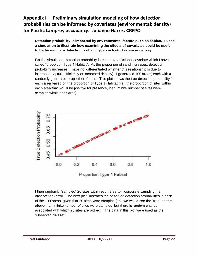
Appendix II – Preliminary simulation modeling of how detection probabilities can be informed by covariates (environmental; density) for Pacific Lamprey occupancy. Julianne Harris, CRFPO

Detection probability is impacted by environmental factors such as habitat. I used

a simulation to illustrate how examining the effects of covariates could be useful

to better estimate detection probability, if such studies are underway.

For the simulation, detection probability is related to a fictional covariate which I have

called “proportion Type 1 Habitat”. As the proportion of sand increases, detection

probability increases (I have not differentiated whether this relationship is due to

increased capture efficiency or increased density). I generated 100 areas, each with a

randomly generated proportion of sand. This plot shows the true detection probability for

each area based on the proportion of Type 1 Habitat (i.e., the proportion of sites within

each area that would be positive for presence, if an infinite number of sites were

sampled within each area).

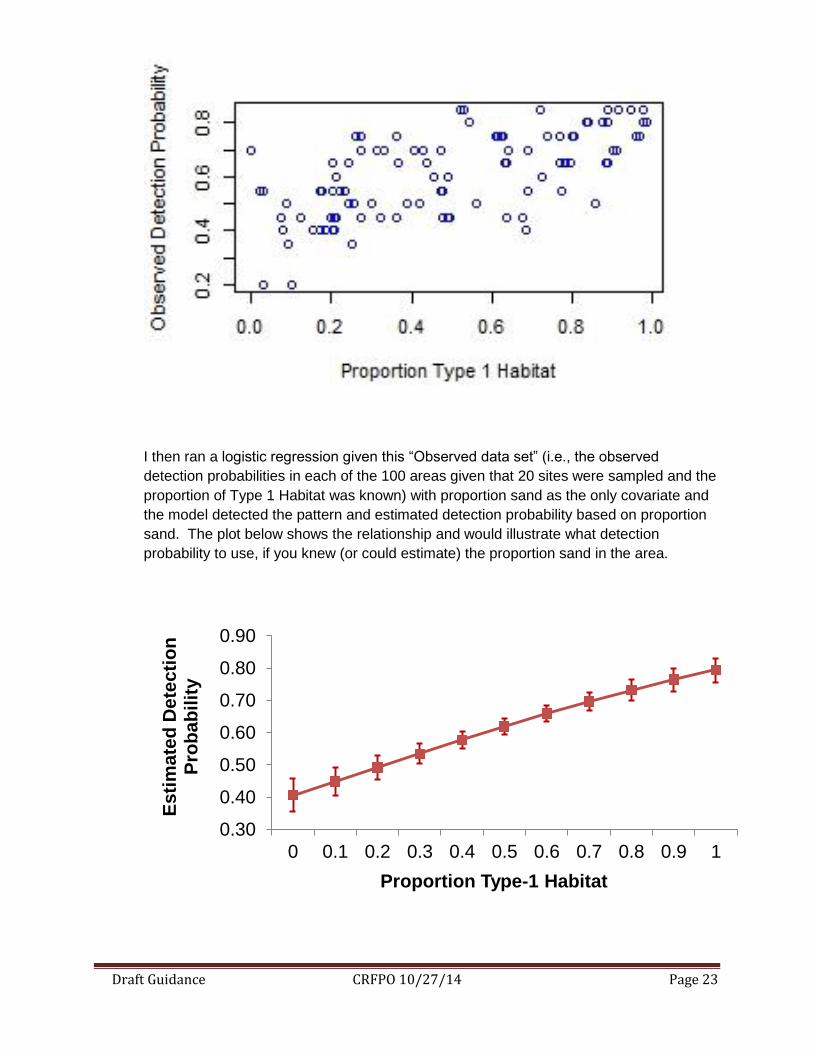
I then randomly “sampled” 20 sites within each area to incorporate sampling (i.e.,

observation) error. The next plot illustrates the observed detection probabilities in each

of the 100 areas, given that 20 sites were sampled (i.e., we would see the “true” pattern

above if an infinite number of sites were sampled, but there is random chance

associated with which 20 sites are picked). The data in this plot were used as the

“Observed dataset”.


I then ran a logistic regression given this “Observed data set” (i.e., the observed

detection probabilities in each of the 100 areas given that 20 sites were sampled and the

proportion of Type 1 Habitat was known) with proportion sand as the only covariate and

the model detected the pattern and estimated detection probability based on proportion

sand. The plot below shows the relationship and would illustrate what detection

probability to use, if you knew (or could estimate) the proportion sand in the area.

0.30

0.40

0.50

0.60

0.70

0.80

0.90

0 0.1 0.2 0.3 0.4 0.5 0.6 0.7 0.8 0.9 1

Es

tim

ate

d D

ete

cti

on

P

rob

ab

ilit

y

Proportion Type-1 Habitat


What this exercise shows is that if multiple studies to estimate detection probability

included measurement of habitat covariates, we could model the relationship between

habitat covariates and detection probability and then have a better understanding of

what our detection probability should be in new un-sampled areas, if we know something

about the habitat there. The selection of 20 sites to estimate detection probability was

randomly—the number needed would be based on what the true detection probability

range really was, but would not need to be the same for all studies to evaluate the

relationship. There would also not need to be 100 areas examined. Similarly to the

number of sites, the number of areas that would need to be examined would depend on

the magnitude of variability and the actual relationship between the covariate and

detection probability. Overall, however, this is the kind of analysis that would require

multiple groups to sample multiple areas in a standardized fashion, so that the data

could be combined for such an analysis.


Appendix III – Steps for Occupancy Sampling: A Mock Example in the Tualatin Basin. Julianne Harris, Gregory Silver, Jeffrey Jolley – CRFPO

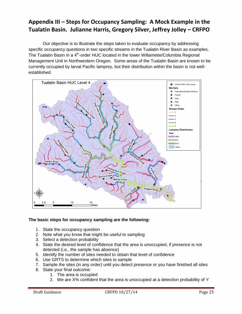
Our objective is to illustrate the steps taken to evaluate occupancy by addressing

specific occupancy questions in two specific streams in the Tualatin River Basin as examples.

The Tualatin Basin in a 4th-order HUC located in the lower Willamette/Columbia Regional

Management Unit in Northwestern Oregon. Some areas of the Tualatin Basin are known to be

currently occupied by larval Pacific lamprey, but their distribution within the basin is not well-

established.

The basic steps for occupancy sampling are the following:

1. State the occupancy question 2. Note what you know that might be useful to sampling 3. Select a detection probability 4. State the desired level of confidence that the area is unoccupied, if presence is not

detected (i.e., the sample has absence) 5. Identify the number of sites needed to obtain that level of confidence 6. Use GRTS to determine which sites to sample 7. Sample the sites (in any order) until you detect presence or you have finished all sites 8. State your final outcome:

1. The area is occupied 2. We are X% confident that the area is unoccupied at a detection probability of Y


Tualatin Mock Example:

Our occupancy questions are related to two 3rd order streams in the Tualatin Basin:

Gales Creek and Fanno Creek, but we started by estimating detection probability in West Fork

Dairy Creek, another third order stream in the Tualatin Basin known to be occupied by larval

Pacific lamprey. Estimating or selecting a detection probability in a similar system (i.e., a similar

3rd order stream in the same basin) with known occupancy is useful, but not always possible.

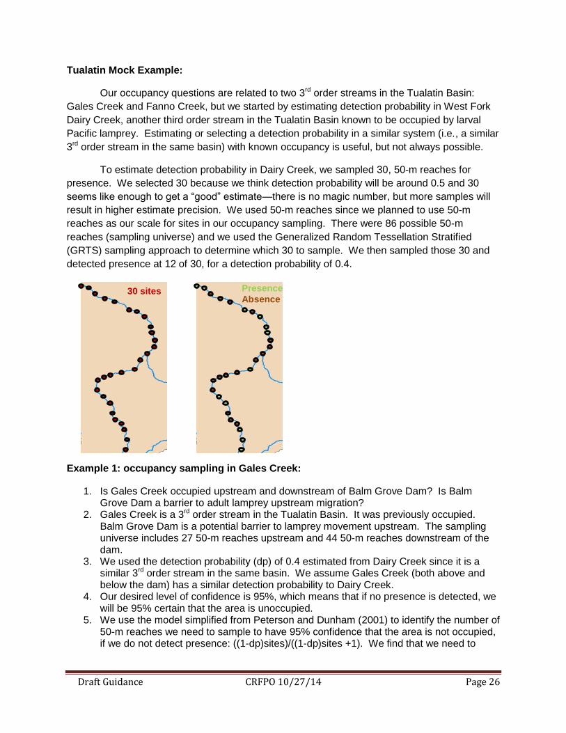
To estimate detection probability in Dairy Creek, we sampled 30, 50-m reaches for

presence. We selected 30 because we think detection probability will be around 0.5 and 30

seems like enough to get a “good” estimate—there is no magic number, but more samples will

result in higher estimate precision. We used 50-m reaches since we planned to use 50-m

reaches as our scale for sites in our occupancy sampling. There were 86 possible 50-m

reaches (sampling universe) and we used the Generalized Random Tessellation Stratified

(GRTS) sampling approach to determine which 30 to sample. We then sampled those 30 and

detected presence at 12 of 30, for a detection probability of 0.4.

Example 1: occupancy sampling in Gales Creek:

1. Is Gales Creek occupied upstream and downstream of Balm Grove Dam? Is Balm Grove Dam a barrier to adult lamprey upstream migration?

2. Gales Creek is a 3rd order stream in the Tualatin Basin. It was previously occupied. Balm Grove Dam is a potential barrier to lamprey movement upstream. The sampling universe includes 27 50-m reaches upstream and 44 50-m reaches downstream of the dam.

3. We used the detection probability (dp) of 0.4 estimated from Dairy Creek since it is a similar 3rd order stream in the same basin. We assume Gales Creek (both above and below the dam) has a similar detection probability to Dairy Creek.

4. Our desired level of confidence is 95%, which means that if no presence is detected, we will be 95% certain that the area is unoccupied.

5. We use the model simplified from Peterson and Dunham (2001) to identify the number of 50-m reaches we need to sample to have 95% confidence that the area is not occupied, if we do not detect presence: ((1-dp)sites)/((1-dp)sites +1). We find that we need to

30 sites Presence

Absence


sample at 6 50-m reaches to have at least 95% confidence that the area is unoccupied, if presence is not detected (if presence is detected, the area is occupied).

# of sites Probability that the area is occupied, but presence will not be detected

Probability that the area is unoccupied

1 0.38 0.62

2 0.26 0.74

3 0.18 0.82

4 0.11 0.89

5 0.07 0.93

6 0.04 0.96

7 0.03 0.97

8 0.02 0.98

9 0.01 0.99

10 0.01 0.99

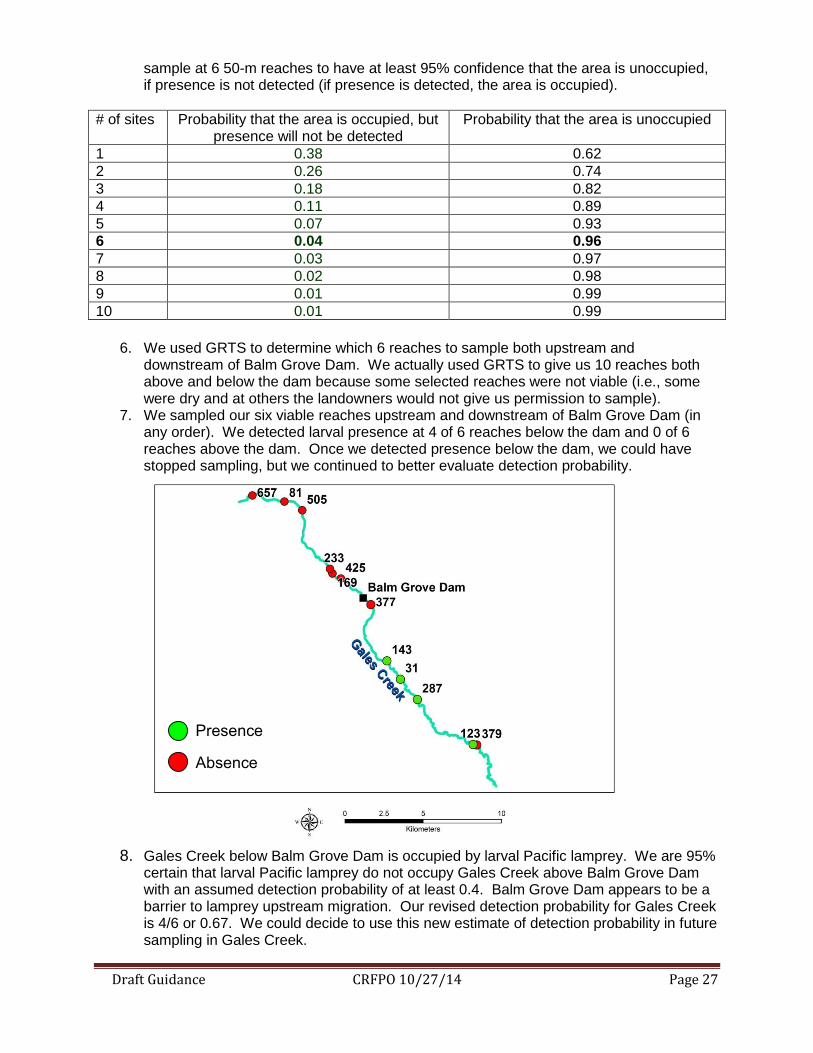
6. We used GRTS to determine which 6 reaches to sample both upstream and downstream of Balm Grove Dam. We actually used GRTS to give us 10 reaches both above and below the dam because some selected reaches were not viable (i.e., some were dry and at others the landowners would not give us permission to sample).

7. We sampled our six viable reaches upstream and downstream of Balm Grove Dam (in any order). We detected larval presence at 4 of 6 reaches below the dam and 0 of 6 reaches above the dam. Once we detected presence below the dam, we could have stopped sampling, but we continued to better evaluate detection probability.

8. Gales Creek below Balm Grove Dam is occupied by larval Pacific lamprey. We are 95%

certain that larval Pacific lamprey do not occupy Gales Creek above Balm Grove Dam with an assumed detection probability of at least 0.4. Balm Grove Dam appears to be a barrier to lamprey upstream migration. Our revised detection probability for Gales Creek is 4/6 or 0.67. We could decide to use this new estimate of detection probability in future sampling in Gales Creek.

Presence

Absence


Example 2: occupancy sampling in Fanno Creek:

1. Is Fanno Creek occupied by larval Pacific lamprey? Has the distribution within the Tualatin Basin changed from historic levels?

2. Fanno Creek is a 3rd order stream in the Tualatin Basin. We know that it was previously occupied by larval Pacific lamprey, but the current status is unknown (previous occupancy data is greater than 10 years old). There are 36, 50-m reaches in Fanno Creek (sampling universe).

3. We used a detection probability of 0.4, since that was the detection probability found during estimation in Dairy Creek. We did not use the estimate derived from occupancy sampling in Gales Creek, although it was also a 3rd order stream in the same basin for two reasons: 1) the detection probability from Dairy Creek has higher precision (i.e., estimated from 30 reaches rather than 6) and 2) the detection probability from Dairy Creek is more conservative.

4. The desired level of confidence again is 95%. 5. We used the same Peterson and Dunham (2001) model as used for Gales Creek and

since we used the same estimate of detection probability, we again got that we needed to sample 6 reaches (see table from above).

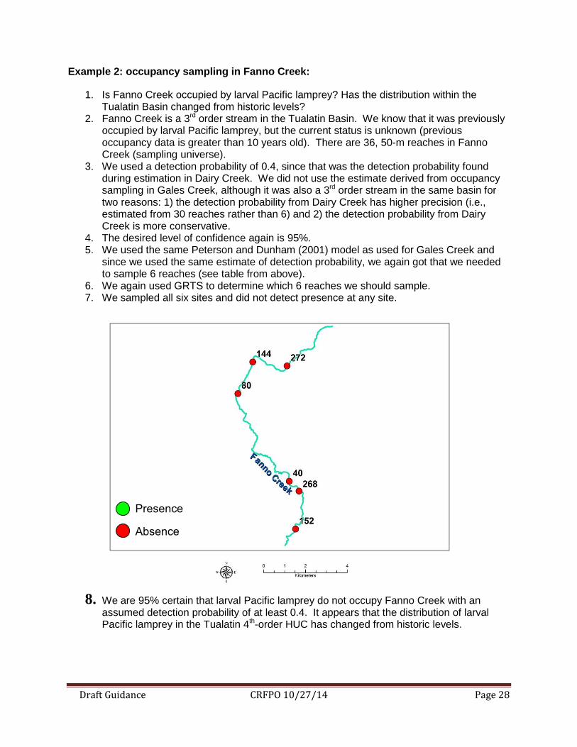
6. We again used GRTS to determine which 6 reaches we should sample. 7. We sampled all six sites and did not detect presence at any site.

8. We are 95% certain that larval Pacific lamprey do not occupy Fanno Creek with an assumed detection probability of at least 0.4. It appears that the distribution of larval Pacific lamprey in the Tualatin 4th-order HUC has changed from historic levels.

Presence

Absence

guidance for pacific lamprey distribution and occupancy sampling€¦ · · 2015-06-08guidance...

Documents