White-headed Woodpecker occupancy in the Pacific Northwest Region (USFS

R6) FINAL

2017 Progress Report

January 2017

Quresh S. Latif1, Vicki Saab1, Kim Mellen-McLean3, Jon Dudley2

USFS Rocky Mountain Research Station, Bozeman, MT1 and Boise, Idaho2; USFS Pacific

Northwest Region3

Report Highlights

Six years (2011–2016) of regional occupancy monitoring was completed for White-

headed Woodpeckers (WHWO) in the Pacific Northwest Region (Oregon and

Washington) as planned.

We summarize resulting data and provide estimates for yearly transect occupancy rates

using occupancy models.

We also provide descriptive statistics for key remotely sensed and field-measured

environmental attributes at survey points (along transects) with and without WHWO

detections.

Finally, we provide guidance for potential future monitoring efforts needed to measure

long-term population trends drawing upon an analysis of the timing of detections within

surveys (presented here) and results from a simulation study (Latif et al. In Review).

WHWO were detected consistently at transects in each of three sub-regions (East

Cascades, Blue Mountains, and North Cascades). We did not find any indication of

obvious population trends, but we could not draw meaningful conclusions regarding

trends given data limitations and the short timeframe of sampling.

Environmental conditions associated with point-level WHWO detections were consistent

with habitat relationships documented in previous studies.

For potential future regional monitoring aimed at quantifying long-term population

trends, we recommend four main adjustments to the monitoring protocol implemented in

2011–2016: 1) implement a single-survey approach with auxiliary sampling to estimate

within-survey detectability while (possibly) conducting repeat surveys during some years

for documenting shifts in breeding phenology due to climate change, 2) monitor more

transects with fewer [4] points each arranged in a square configuration, 3) monitor

transects in clusters with member transects spaced sufficiently for statistical

independence to reduce travel time between transects and thereby allow more transects to

be monitored, 4) depending upon questions of interest, possibly implement a panel design

whereby a rotating subset of transects would be surveyed each year to allow monitoring a

larger overall sample.

INTRODUCTION

The White-headed Woodpecker is a regional endemic species of the Inland Northwest and

California. This woodpecker may be particularly vulnerable to environmental change because it

occupies a limited distribution and it has narrow habitat requirements. They are year-round

residents of dry coniferous forests, typically found in open ponderosa pine forests with mature,

cone-producing trees that provide seasonal foraging resources, and snags and stumps that

provide nest cavity substrates. Mature, open, ponderosa pine habitat has declined more

dramatically than any other forested habitat of the Interior Pacific Northwest (Wisdom et al.

2002). Dry forest habitat occupied by White-headed Woodpeckers is the target of most

restoration and fuels reduction projects in the USFS Pacific Northwest Region, which have the

potential for beneficial or negative effects on their habitat. Concerns for this species provided the

incentive to establish regional monitoring for a better understanding of habitat needs and to

inform restoration projects and fuels prescriptions.

Regional occupancy-based monitoring of White-headed Woodpeckers (Picoides

albolarvatus; hereafter WHWO) across the interior Pacific Northwest Region was initiated in

2011. The survey protocol was based on results from 16 transects from a pilot study in 2010.

Call-broadcast surveys were conducted each year at 300 survey points arranged along 30

transects distributed across potential habitat. Surveyors repeatedly visited transects twice per

year to provide data for estimating detectability and modeling occupancy (MacKenzie et al.

2003, Royle and Kéry 2007). Additionally, habitat was measured at survey points twice over the

study period (once in 2011–2013 and again in 2014–2016) to allow analysis of habitat

relationships with WHWO occurrence. This report follows six years of data collection (2011–

2016), which completes the currently funded regional monitoring effort (Mellen-McLean et al.

2015).

In this report, we provide a final summary and analysis of regional monitoring data to

inform future monitoring efforts. We present 1) yearly transect occupancy estimates and an

overall estimate of detectability, 2) a summary of which transects were occupied during the study

period, 3) a comparison of environmental conditions at survey points with and without WHWO

detections, and 4) an analysis of the timing of detections. We synthesize ecological information

and knowledge gained from these efforts, and provide a suggested sampling design for continued

regional long-term monitoring to document population trends.

METHODS

We estimated yearly occupancy probabilities over the study period (2011–2016) and overall

detectability using an occupancy model fitted to transect detection data. We modeled the

probability of transect occupancy on a logit scale: logit(ψt) = bt, where bt varied as a fixed effect

of year t. We modeled the occupancy state of transect i in year t as a function of the occupancy

probability: zit ~ Bernoulli(ψt). For transect detection data, yitk = 1 when ≥ 1 WHWO was

detected at any survey point along transect i in year t during visit k. We modeled detection data

as yitk ~ Bernoulli(p × zit), where p is the probability of detecting WHWO when surveying an

occupied transect. We formulated this model using Bayesian methods (Royle and Kéry 2007)

fitted using JAGS (v. 4.2.0; Plummer 2003) programmed from R (v. 3.3.2; R Core Team 2017)

via the R2jags package (Su and Yajima 2014). We used independent non-informative priors for

all parameters and sampled posterior parameter distributions with 4 parallel MCMC chains. We

verified sufficient sampling and chain convergence by checking neffective ≥ 100 and �̂� ≤ 1.1,

respectively (Gelman and Hill 2007).

We summarized and tabulated environmental data at survey points along regional

monitoring transects. We summarized data for 5 remotely sensed and 7 field-collected variables

describing topography, forest structure, and tree species composition (Table 1). Relevance of

these environmental attributes, data sources (remotely sensed), measurement protocols (field-

collected), and relationships with WHWO occurrence are described in detail elsewhere

(Wightman et al. 2010, Hollenbeck et al. 2011, Latif et al. 2014, 2015). In this report, we provide

basic summary statistics for survey points with and without WHWO detections over the study

period (2011–2016) to describe the data generated from regional monitoring and inform future

analyses. We conducted two-sample t-tests to identify variables with statistically significant

differences in means (α = 0.05) between points with versus without WHWO detections.

We analyzed the timing of detections to inform survey duration for future WHWO

monitoring. Considerations of survey duration were motivated by simulation study showing

greater effectiveness of single surveys (accompanied by auxiliary sampling, e.g., detection

timings, to inform within-survey detectability) over repeat surveys for monitoring population

trends (Latif et al. In Review). In 2012–2016, surveyors recorded the time remaining until point-

survey completion (max = 4.5 min) when WHWO were first detected. We examined the

distribution of detection timings classified into 1.5-min sub-periods (3 sub-periods per survey) to

qualitatively assess the potential need for longer surveys. We reasoned that if detections were

primarily recorded during sub-periods 1 or 2 (first 3 min), lengthening survey duration would be

unnecessary. Conversely, a similar or larger proportion of detections recorded in sub-period 3

relative to sub-periods 1 or 2 would suggest longer surveys are needed to allow sufficient

chances of detecting WHWO where present.

We supplemented qualitative assessment of detection timing data with model-based

estimates of perceptibility, pp – the probability of perceiving WHWO during a survey given their

physical presence (e.g., Rota et al. 2009, sensu Latif et al. 2016; for modeling details, see

Appendix A). We modeled pp for 1.5 min survey sub-periods and derived estimates for entire

surveys (p*p, R = 1 – [1 - pp]R, where R = survey duration in minutes). We considered p*p, R ≲ 0.9

indicative of low perceptibility and a need for longer surveys (MacKenzie and Royle 2005). For

model-based analysis, we used boot-strapping to fill in missing detection timing data, i.e., we

resampled existing data to fill in missing data for 30 boot-strapped datasets, and then

summarized posterior estimates of within-survey detectability across boot-strapped data. We

used qualitative and quantitative assessments of detection timings, along with other

considerations, to inform sampling design for potential future monitoring.

We evaluated timing data for both point- and transect-level detections. At the transect-

level, we considered WHWO detected when detected at ≥ 1 point and the timing of a detection

equal to the earliest point detection timing along a given transect. We evaluated transect

detection timings for full-length transects (10 points each) and for reduced-length transects (4

points each; recommended for potential future monitoring by Latif et al. In Review). When

analyzing detection timings for reduced-length transects, we treated the first and last four survey

points along each 10-point transect as separate transects.

RESULTS

Surveyors detected WHWO during 248 surveys at 123 points along 22 transects over the 6-year

study period. WHWO were detected in each of 3 sub-regions representing different mountain

ranges in every year of the study period (Figure 1). Yearly occupancy probability estimates

ranged 0.46–0.67 and suggested no obvious population trends (Figure 2).

Environmental values differed between survey points with and without WHWO

detections for 3 remotely-sensed and 3 field-measured variables (Table 2). Points where WHWO

were detected had lower canopy cover at 1-ha and 314-ha scales and more ponderosa pine-

dominated forest than points where WHWO were never detected. Points with WHWO detections

also had fewer medium-diameter trees and snags, but more large ponderosa pine trees than points

without detections.

Detection timing data were associated with 171 point detections, 103 10-point (full

length) transect detections, and 101 4-point (reduced length) transect detections. Detections were

recorded at similar frequencies during earlier versus later 1.5-min survey sub-periods (Figure 3).

Model-based estimates indicated low perceptibility for when surveying either full-length 10-

point transects or reduced-length 4-point transects with the current 4.5-min survey duration, and

suggested longer surveys may be needed for sufficient perceptibility (Table 3).

DISCUSSION

Regional occupancy-based monitoring has contributed to current knowledge of white-headed

woodpecker population status. Early research in the Blue Mountains (late 1970s – early 1980s)

found white-headed woodpecker to be relatively common, whereas subsequent research (early

2000s) in the same area found no WHWO (Altman 2000, Bull 1980, Nielsen-Pincus 2005).

Regional monitoring in 2011–2016 show persistent WHWO occurrence at several widely

distributed locations in the Blue Mountains. More generally, monitoring data suggest broad

persistence throughout the region. Long-term population trends, however, will remain uncertain

without more extensive monitoring (Latif et al In Review).

Environmental conditions associated with WHWO detections during regional monitoring

were largely consistent with relationships quantified in previous work (Wightman et al. 2010,

Hollenbeck et al. 2011, Latif et al. 2014, 2015). White-headed woodpeckers favor large-diameter

ponderosa pine for nesting and foraging, such that breeding habitat favors ponderosa pine-

dominated forests. Nesting habitat is also associated with canopy mosaics whereby nests are

located in canopy openings adjacent to more closed-canopy forests thought to provide foraging

habitat (Hollenbeck et al. 2011, Latif et al. 2015). Lower canopy cover and fewer medium trees

and snags at point detection locations reported here likely reflect nesting preferences for canopy

openings. Our simplified univariate analyses were limited for discerning previously documented

scale-specific relationships with canopy cover reflecting associations with canopy mosaics (Latif

et al. 2015). More sophisticated model-based analyses of regional monitoring data hinted at these

relationships but were still limited by the ambiguity regarding whether point detections signify

habitat use for nesting versus foraging (Latif et al. 2014). Nevertheless, longer-term monitoring

could complement published studies of nesting distributions by quantifying habitat relationships

with occupancy dynamics (e.g., Kéry et al. 2013).

Given interest in extending monitoring to measure population trends, simulations indicate

single surveys (i.e., 1 visit per year) accompanied with detection timings would provide more

statistical power for observing trends and better trend estimates than the repeat-survey approach

implemented in 2011–2016 (Latif et al. In Review). Our analysis of detection timing data

indicate a need for a longer survey duration, however, to provide sufficient detectability with a

single-survey approach. MacKenzie and Royle (2005) provide optimal numbers of replicate

surveys given various levels of occupancy and detectability. Applying their recommendations to

our estimates of perceptibility and probability of species presence (Table 3), one might infer

optimal survey durations of ~9–13 min depending on transect length. Published

recommendations are based on known occupancy and detectability (MacKenzie and Royle

2005), however, whereas our estimates are uncertain and likely biased due to insufficient

detectability (MacKenzie et al. 2002, McKann et al. 2013).

Given these uncertainties, we recommend initially conducting 10-min surveys and

subsequently adjusting survey duration depending upon the distribution of detection timings. As

a rule of thumb, the frequency of new detections should ideally drop noticeably in the final sub-

period immediately preceding the end of the survey. If the frequency of new detections drops

earlier, surveys can be shortened, whereas if no drop is observed, surveys would need to be

lengthened. Quantitative analyses based on published recommendations and tools (MacKenzie

and Royle 2005, Bailey et al. 2007) should ideally supplement qualitative evaluation of detection

timings to identify an optimal survey length. Whereas we estimated perceptibility for 1.5-min

sub-periods, perceptibility estimated for shorter (e.g., 30-sec) sub-periods could inform finer

resolution assessment of optimal survey length (for analysis details, see Appendix A).

FUTURE MONITORING

Based on results reported here and from a separate simulation study (Latif et al. In Review), we

have several recommendations for adjusting the protocol applied in 2011–2016 (Mellen-McLean

et al. 2015) for monitoring regional WHWO population trends.

1. We recommend switching to a single-survey approach to monitoring. A single-survey

protocol would allow monitoring of more transects over a broader area, likely improving

statistical power for observing trends and reducing error of estimated trends with respect

to actual trends in population size (Latif et al. In Review). We provide two caveats to our

recommendation for single surveys. First, auxiliary sampling of detection timing would

be needed to estimate within-survey detectability (i.e., perceptibility, sensu Latif et al.

2016), and preliminary assessment of optimal survey duration would be strongly advised

as described above. Second, the single survey approach relies on consistent

responsiveness of WHWOs to call broadcasts across years, and because responsiveness

varies over the nesting period (Mellen-McLean 2015), this approach also requires

maintaining survey timing in relation to breeding phenology. Shifts in breeding

phenology resulting from climate change and consequent changes in responsiveness to

broadcast calls could cause spurious observations of apparent population trends with

single surveys. Repeat surveys conducted during some years (e.g., once in 3–5 years),

along with nesting data, could help uncover shifts in breeding phenology. Alternatively,

analysis of single-survey data could test for relationships between occupancy estimates

and seasonal timing.

2. We also recommend monitoring shorter transects of 4 points each arranged as a square.

Such transects would offer several advantages over the 10-point straight-line transects

monitored in 2011–2016. Shorter transects can improve statistical power for observing

trends by allow monitoring of more transects (Latif et al. In Review). A 4-point square

transect would also align more closely to the size and shape of a single home range,

which would minimize variability in local abundance among occupied transects and

thereby provide occupancy estimates that better track abundance (Efford and Dawson

2012, Latif et al. In Review). Finally, the route taken to survey a square transect would

form a loop, reducing the travel time back to the surveyor’s field vehicle, potentially

allowing surveys of multiple transects per day.

3. We recommend monitoring transects in clusters with member transects spaced

sufficiently to ensure sampling of different individuals (e.g., 5–10 km apart). Such an

arrangement would allow more transects to be monitored by reducing travel time between

transects. Additionally, occupancy models that allow random variation among clusters

(i.e., random effects of cluster) could reveal spatial variability in population size (indexed

by occupancy rates) and trends.

4. Depending upon questions of interest, we suggest considering a panel design, whereby a

rotating subset of transects would be surveyed each year. A panel design can improve

statistical power for observing population trends by allowing monitoring of a larger

overall sample of transects (Latif et al. In Review). By monitoring each transect less

frequently, however, there would be less opportunity for quantifying occupancy

dynamics (i.e., colonization, extinction, and turnover; MacKenzie et al. 2003, Bailey et

al. 2007, Kéry et al. 2013). Thus, the value of a panel design would depend on which

aspects of WHWO population dynamics are of greatest interest. For example, if we are

interested in understanding variation in long-term trends among sub-regions (East

Cascades, Blue Mountains, North Cascades), a panel design may be valuable to boost the

number of transects surveyed within each sub-region. If instead we are interested in

understanding how suspected environmental drivers affect occupancy dynamics at

individual transects, we may be better off surveying a smaller set of transects every year.

LITERATURE CITED

Altman, B. 2000. Conservation strategy for landbirds in the northern Rocky Mountains of eastern

Oregon and Washington. Version 1.0. Oregon and Washington Partners in Flight.

Unpubl. Rpt., 128 pp.

Bailey, L. L., J. E. Hines, J. D. Nichols, and D. I. MacKenzie. 2007. Sampling design trade-offs

in occupancy studies with imperfect detection: examples and software. Ecological

Applications 17:281-290.

Bull, E.L. 1980. Resource Partitioning among woodpeckers in northeastern Oregon. PhD

Dissertation, University of Idaho, Moscow. 109 pp.

Efford, M. G., and D. K. Dawson. 2012. Occupancy in continuous habitat. Ecosphere 3:article

32.

Gelman, A., and J. Hill. 2007. Data analysis using regression and multilevel/ hierarchical

models. Cambridge University Press, New York, NY.

Hollenbeck, J. P., V. A. Saab, and R. W. Frenzel. 2011. Habitat suitability and nest survival of

White-headed Woodpeckers in unburned forests of Oregon. Journal of Wildlife

Management 75:1061-1071.

Kéry, M., G. Guillera-Arroita, and J. J. Lahoz-Monfort. 2013. Analysing and mapping species

range dynamics using occupancy models. Journal of Biogeography 40:1463-1474.

Landscape Ecology Modeling, Mapping, and Analysis (LEMMA). (2012)

http://www.fsl.orst.edu/lemma/splash.php. last accessed March 2012.

Latif, Q. S., M. M. Ellis, and C. L. Amundson. 2016. A broader definition of occupancy:

Comment on Hayes and Monfils. The Journal of Wildlife Management 80:192-194.

Latif, Q.S., M.M. Ellis, V.A. Saab, and K. Mellen-McLean. In Review. Simulations inform

design of regional occupancy-based monitoring for a sparsely distributed, territorial

species. Methods in Ecology and Evolution.

Latif, Q.S., V.A. Saab, K. Mellen-McLean, J.G. Dudley. 2014. Occupancy trends and patterns

for White-headed Woodpecker in the Pacific Northwest Region. 2014 Progress Report,

USFS Region 6.

Latif, Q. S., V. A. Saab, K. Mellen-Mclean, and J. G. Dudley. 2015. Evaluating habitat

suitability models for nesting white-headed woodpeckers in unburned forest. The Journal

of Wildlife Management 79:263-273.

MacKenzie, D. I., J. D. Nichols, J. E. Hines, M. G. Knutson, and A. B. Franklin. 2003.

Estimating site occupancy, colonization, and local extinction when a species is detected

imperfectly. Ecology 84:2200-2207.

MacKenzie, D. I., J. D. Nichols, G. B. Lachman, S. Droege, J. A. Royle, and C. A. Langtimm.

2002. Estimating site occupancy rates when detection probabilities are less than one.

Ecology 83:2248-2255.

MacKenzie, D. I., and J. A. Royle. 2005. Designing occupancy studies: general advice and

allocating survey effort. Journal of Applied Ecology 42:1105-1114.

McKann, P. C., B. R. Gray, and W. E. Thogmartin. 2013. Small sample bias in dynamic

occupancy models. The Journal of Wildlife Management 77:172-180.

Mellen-McLean, K., V. Saab, B. Bresson, A. Wales, and K. VanNorman. 2015. White-headed

Woodpecker Monitoring Strategy and Protocols for the Pacific Northwest Region. v1.3.

U.S. Forest Service, Pacific Northwest Region, Portland, OR. 34 pp.

Nielsen-Pincus, N. 2005. Nest site selection; nest success, and density of selected cavity-nesting

birds in northeastern Oregon with a method for improving accuracy of density estimates.

M.S. Thesis. University of Idaho, Moscow. 96 pp.

Plummer, M. 2003. JAGS: A program for analysis of Bayesian graphical models using Gibbs

sampling.in Proceedings of the 3rd International Workshop on Distributed Statistical

Computing (DSC 2003), March 20-22, Vienna, Austria.

R Core Team. 2017. R: A language and environment for statistical computing. R Foundation for

Statistical Computing, Vienna, Austria. <http://www.R-project.org>.

Rota, C. T., R. J. Fletcher Jr, R. M. Dorazio, and M. G. Betts. 2009. Occupancy estimation and

the closure assumption. Journal of Applied Ecology 46:1173-1181.

Royle, J. A., and M. Kéry. 2007. A Bayesian state-space formulation of dynamic occupancy

models. Ecology 88:1813-1823.

Su, Y.-S., and M. Yajima. 2014. R2jags: A package for running jags from R. R package version

3.3.0. http://CRAN.R-project.org/package=R2jags.

Wightman, C. S., V. A. Saab, C. Forristal, K. Mellen-McLean, and A. Markus. 2010. White-

headed Woodpecker nesting ecology after wildfire. Journal of Wildlife Management

74:1098-1106.

Wisdom, M. J., R. S. Holthausen, B. C. Wales, C. D. Hargis, V. A. Saab, D. C. Lee, W. J. Hann,

R. D. Terrell, M. M. Rowland, W. J. Murphy, and M. R. Eames. 2002. Source habitats

for terrestrial vertebrates of focus in the interior Columbia basin: broadscale trends and

management implications—Volume 1, Overview. Gen. Tech. Rep. PNW-GTR-485.

Portland, OR: U.S. Department of Agriculture, Forest Service, Pacific Northwest

Research Station. 3 vol. (Quigley, Thomas M., tech. ed.; Interior Columbia Basin

Ecosystem Management Project: scientific assessment).

TABLES

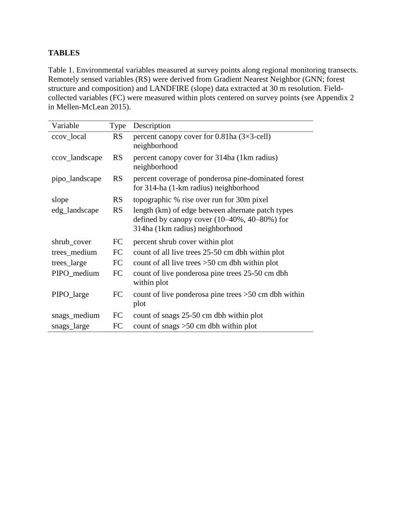
Table 1. Environmental variables measured at survey points along regional monitoring transects.

Remotely sensed variables (RS) were derived from Gradient Nearest Neighbor (GNN; forest

structure and composition) and LANDFIRE (slope) data extracted at 30 m resolution. Field-

collected variables (FC) were measured within plots centered on survey points (see Appendix 2

in Mellen-McLean 2015).

Variable Type Description

ccov_local RS percent canopy cover for 0.81ha (3×3-cell)

neighborhood

ccov_landscape RS percent canopy cover for 314ha (1km radius)

neighborhood

pipo_landscape RS percent coverage of ponderosa pine-dominated forest

for 314-ha (1-km radius) neighborhood

slope RS topographic % rise over run for 30m pixel

edg_landscape RS length (km) of edge between alternate patch types

defined by canopy cover (10–40%, 40–80%) for

314ha (1km radius) neighborhood

shrub_cover FC percent shrub cover within plot

trees_medium FC count of all live trees 25-50 cm dbh within plot

trees_large FC count of all live trees >50 cm dbh within plot

PIPO_medium FC count of live ponderosa pine trees 25-50 cm dbh

within plot

PIPO_large FC count of live ponderosa pine trees >50 cm dbh within

plot

snags_medium FC count of snags 25-50 cm dbh within plot

snags_large FC count of snags >50 cm dbh within plot

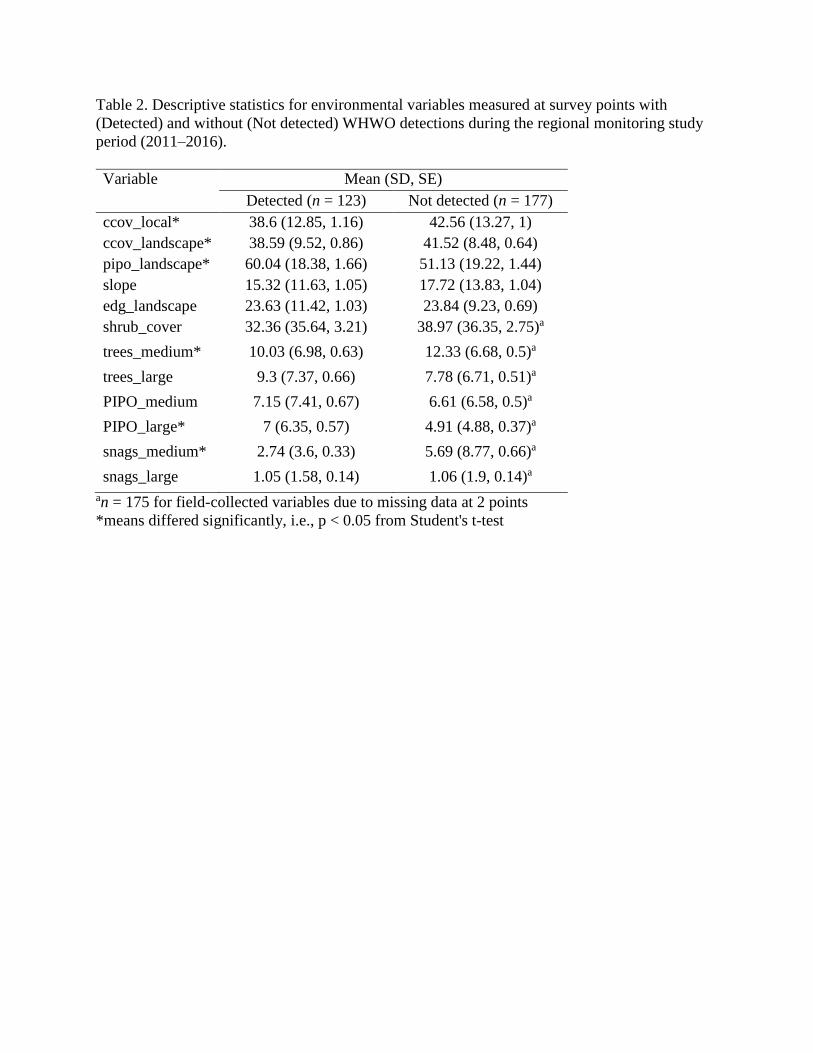
Table 2. Descriptive statistics for environmental variables measured at survey points with

(Detected) and without (Not detected) WHWO detections during the regional monitoring study

period (2011–2016).

Variable Mean (SD, SE)

Detected (n = 123) Not detected (n = 177)

ccov_local* 38.6 (12.85, 1.16) 42.56 (13.27, 1)

ccov_landscape* 38.59 (9.52, 0.86) 41.52 (8.48, 0.64)

pipo_landscape* 60.04 (18.38, 1.66) 51.13 (19.22, 1.44)

slope 15.32 (11.63, 1.05) 17.72 (13.83, 1.04)

edg_landscape 23.63 (11.42, 1.03) 23.84 (9.23, 0.69)

shrub_cover 32.36 (35.64, 3.21) 38.97 (36.35, 2.75)a

trees_medium* 10.03 (6.98, 0.63) 12.33 (6.68, 0.5)a

trees_large 9.3 (7.37, 0.66) 7.78 (6.71, 0.51)a

PIPO_medium 7.15 (7.41, 0.67) 6.61 (6.58, 0.5)a

PIPO_large* 7 (6.35, 0.57) 4.91 (4.88, 0.37)a

snags_medium* 2.74 (3.6, 0.33) 5.69 (8.77, 0.66)a

snags_large 1.05 (1.58, 0.14) 1.06 (1.9, 0.14)a

an = 175 for field-collected variables due to missing data at 2 points

*means differed significantly, i.e., p < 0.05 from Student's t-test

Table 3. Posterior parameter estimates from analysis of detection timing data to inform survey

duration for white-headed woodpecker regional monitoring (for model details, see Appendix A).

pa × Ψ2011–2016 = the unconditional probability of ≥ 1 white-headed woodpecker being physically

present during a given transect survey. pp = probability of perceiving white-headed woodpecker

within a 1.5-min survey sub-period given their physical presence. p*p, t = the overall

perceptibility estimate over a survey period of t minutes.

Parameter median estimates (95th %-iles)

10-point transects 4-point transects

pp 0.32 (0.25, 0.42) 0.2 (0.13, 0.33)a

pa × Ψ2011–2016 0.57 (0.36, 0.79) 0.4 (0.2, 0.74)

p*p, 4..5 0.68 (0.57, 0.8) 0.5 (0.34, 0.7)

p*p, 6 0.78 (0.68, 0.88) 0.6 (0.43, 0.8)

p*p, 9 0.9 (0.82, 0.96) 0.75 (0.57, 0.91)

p*p, 10.5 0.93 (0.86, 0.98) 0.8 (0.63, 0.94)

p*p, 13.5 0.97 (0.92, 0.99) 0.87 (0.72, 0.97)

aEven though pp is less for 4-point transects, they are recommended because they provide greater

statistical power to observe population trend and align better with home range size (Latif et al. In

Review). A surveyor is less likely to observe WHWO along a shorter transect, but more transects

can be surveyed.

FIGURES

Figure 1. Locations of transects surveyed yearly to monitor White-headed Woodpeckers across

the Pacific Northwest Region. Transects where WHWO were detected (red) and not detected

(black) are depicted in each year and for the entire 6-year study period.

Figure 2. Mean transect-scale occupancy probabilities (ψ) by year. Occupancy probabilities were

estimated with a model that assumed constant detectability fitted to 2011–2016 regional

monitoring data for white-headed woodpeckers.

Figure 3. Timing of WHWO detections (min) recorded within 4.5 min surveys in 2012–2016.

Detections were recorded at survey points (top panel; n = 171), 10-point (full length) transects

(lower left; n = 103), and 4-point (reduced length) transects (lower right; n = 101).

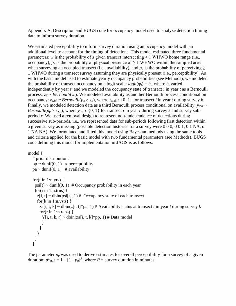
Appendix A. Description and BUGS code for occupancy model used to analyze detection timing

data to inform survey duration.

We estimated perceptibility to inform survey duration using an occupancy model with an

additional level to account for the timing of detections. This model estimated three fundamental

parameters: ψ is the probability of a given transect intersecting ≥ 1 WHWO home range (i.e.,

occupancy), pa is the probability of physical presence of ≥ 1 WHWO within the sampled area

when surveying an occupied transect (i.e., availability), and pp is the probability of perceiving ≥

1 WHWO during a transect survey assuming they are physically present (i.e., perceptibility). As

with the basic model used to estimate yearly occupancy probabilities (see Methods), we modeled

the probability of transect occupancy on a logit scale: logit(ψt) = bt, where bt varied

independently by year t, and we modeled the occupancy state of transect i in year t as a Bernoulli

process: zit ~ Bernoulli(ψt). We modeled availability as another Bernoulli process conditional on

occupancy: za,itk ~ Bernoulli(pa × zit), where za,itk ϵ {0, 1} for transect i in year t during survey k.

Finally, we modeled detection data as a third Bernoulli process conditional on availability: yitkr ~

Bernoulli(pp × za,it), where yitkr ϵ {0, 1} for transect i in year t during survey k and survey sub-

period r. We used a removal design to represent non-independence of detections during

successive sub-periods, i.e., we represented data for sub-periods following first detection within

a given survey as missing (possible detection histories for a survey were 0 0 0, 0 0 1, 0 1 NA, or

1 NA NA). We formulated and fitted this model using Bayesian methods using the same tools

and criteria applied for the basic model with two fundamental parameters (see Methods). BUGS

code defining this model for implementation in JAGS is as follows:

model {

# prior distributions

pp ~ dunif(0, 1) # perceptibility

pa ~ dunif(0, 1) # availability

for(t in 1:n.yrs) {

psi[t] ~ dunif(0, 1) # Occupancy probability in each year

for(i in 1:n.trns) {

z[i, t] ~ dbin(psi[t], 1) # Occupancy state of each transect

for(k in 1:n.vsts) {

za[i, t, k] ~ dbin(z[i, t]*pa, 1) # Availability status at transect i in year t during survey k

for(r in 1:n.reps) {

Y[i, t, k, r] ~ dbin(za[i, t, k]*pp, 1) # Data model

}

}

}

}

}

The parameter pp was used to derive estimates for overall perceptibility for a survey of a given

duration: p*p, R = 1 – [1 - pp]R, where R = survey duration in minutes.