GROUND WATER HYDROLOGY(WRIE – 2136)

Lecture-01: Introduction

Programme: BSc in Water Resources and Irrigation Engineering

Course Objectives

This course is intended to provide :

The basic theories, principles and mathematical model governing sub surface flow

It deals with sub surface storage mechanism and flow pattern

Course outlines

1. Occurrences of Groundwater Ground Water Resources Occurrences of Ground water Unsaturated Zone/Zone of aeration Saturated Zone Aquifers and their characteristics Determination of ground water flow parameter

2. Movement of Ground water Darcy’s law Hydraulic conductivity Hydraulic flow and Transmissivity Flow in anisotropic aquifer Ground water Flow direction Flow nets Flow in relation to groundwater contours

Ground water flow equations

Course outlines

3. Well Hydraulics

Steady Radial flow to a well

Confined aquifer

Unconfined aquifer

Unsteady Radial flow to a well

Confined aquifer

Unconfined aquifer

Unsteady Radial flow to a well in leaky aquifers

Partially penetrating well

Multiple well systems

Well losses and specific capacity

Course outlines

4. Pumping tests of wells

Test wells and observation wells

Performing pumping tests

Methods of Analysis and Interpretation

5. Introduction to ground water modeling

CHAPTER ONE OCCURRENCES OF GROUNDWATER

1.1. Groundwater Resources

Ground Water: is the water that exists in the pore spaces and fractures in rocks and sediments beneath the earth’s surface.

Pore space: the openings between the soil particles

Porosity : the ratio of the pore spaces over the total volume

of the soil

Out of the total volume of water on land, 61% is groundwater

Important for drinking and irrigation

Conti…….

To understand the occurrences and distribution of Gw, it is important to know the hydrologic cycle

Figure 1.1: Groundwater flow in the hydrologic cycle

Conti……

The most favorable areas to ground water:

Existence of favorable geologic structures

Permeable rock zones

Topographically depressed areas

Areas with good ground water recharge possibilities

.

.

.

1.2. Occurrence of Groundwater

Groundwater system is the zone in the earth’s crust

where the open space in the rock is completely filled

with groundwater at a pressure greater than

atmospheric.

Groundwater stretches out below the groundwater

table

Groundwater table is the top most part of

groundwater

=› it may be located near or even at land surface

and not fixed ( i,e it fluctuate seasonally)

Figure 1.2a: Schematic representation of subsurface water in the soil

Two zones can be distinguished in which water occurs in the

ground:

a. The unsaturated zone/ Zone of aeration

b. The saturated zone

Infiltration: The process of water entering into the ground Percolation: Downward transport of water in the unsaturated zone

Capillary rise: The upward transport in the unsaturated zone

Groundwater flow: The flow of water through saturated porous media

Seepage: The out flow from groundwater to surface water

A. Unsaturated Zone/ Zone of aeration Unsaturated Zone (zone of aeration): In this zone the soil pores

are only partially saturated with water

It is marked by the space b/n the land surface and the water table

The zone of aeration has three sub zones:

a. soil water zone: it lies close to the ground surface in the

major root band of the vegetation from which the water is lost

to the atmosphere by evapotranspiration

b. capillary fringe: This zone extends from the water table

upwards to the limit of the capillary rise

c. intermediate zone: it lies b/n the soil water zone and the

capillary fringe

The soil moisture in the zone of aeration is of importance in

agricultural practice and irrigation engineering.

However, this course is concerned only with the saturated

zone

Important conditions in unsaturated zone are;

the wilting point and

the field capacity

Field capacity is the moisture content in the soil a few days

after irrigation or heavy rainfall, when excess water in the

unsaturated zone has percolated

Figure 1.2b: Classification of subsurface water and variation in degree of saturation

b. Saturated Zone Groundwater is the water which occurs in the saturated zone.

All earth materials, from soils to rocks have pore spaces

these pores are completely saturated with water below the groundwater

table or phreatic surface (GWT)

Natural variations in permeability and ease of transmission of groundwater

in d/t saturated geological formations lead to the recognition of:

A. Aquifer: A water-bearing layer for which the porosity and pore size are

sufficiently large which is not only stores water but yields it in sufficient

quantity due to its high permeability.

e.g. sand, gravel layers (Unconsolidated deposits of sand and gravel)

B. Aquitard: It is less permeable geological formation which

may be capable of transmitting water (e.g. sandy clay layer).

It may transmit quantities of water that are significant in

terms of regional groundwater flow

C. Aquiclude: is a geological formation which is essentially

impermeable to the flow of water.

It may be considered as closed to water movement even

though it may contain large amount of groundwater due to

its high porosity (e.g. clay).

D. Aquifuge: is a geological formation which is neither

porous nor permeable.

There are no interconnected openings and hence it cannot

transmit water.

e.g: Massive compacted rock without any fractures is an

aquifuge.

1.2.3. Aquifers and their characteristics

For a description or mathematical treatment of groundwater

flow the geological formation can be schematized into an

aquifer system, consisting of various layers with distinct

different hydraulic properties.

The aquifers are simplified into one of the following types:

i. Unconfined aquifer (phreatic or water table aquifer):

This aquifer consists of a pervious layer underlain by a (semi-)

impervious layer.

it is not completely saturated with water. The upper boundary is

formed by a free water-table (phreatic surface) that is in direct

contact with the atmosphere.

ii. Confined aquifer: it consists of a completely saturated

pervious layer bounded by impervious layers.

There is no direct contact with the atmosphere. The water level in

wells tapping these aquifers rises above the top of the pervious

layer and sometimes even above soil surface (artesian wells).

iii. Semi-confined (Leaky aquifers): consists of a

completely saturated pervious layer, but the upper and/or

lower boundaries are semi-pervious.

They are overlain by aquitard that may have inflow and

outflow through them.

iv. Perched aquifers: These are unconfined aquifers of

isolated in nature.

They are not connected with other aquifers

Figure1.4: Different types of aquifer formations

1.2.4. Determination of groundwater flow parameters

The ff are some of the groundwater flow parameters which are

important in the storage and transmission of water in aquifers:

1. Porosity (n)

The porosity, n is the ratio of volume of the open space in the rock

or soil to the total volume of soil or rock.

(1.1)

Where:

Vv = the pore volume or volume of voids

VT = the total volume of the soil

2. Specific yield (Sy)

The ratio of volume of water in the aquifer which can be

extracted by the force of gravity or by pumping wells to the

total volume of saturated aquifer is called Specific yield (Sy).

(1.2)

Where:

Sy= Specific yield

Vw=the volume of extractible water(except capillary and

hygroscopic water)

VT = the total volume of the soil

1.5b. Specific yield of unconfined aquifer

3. Specific retention (Sr)

The water which is not drained or the ratio of volume of water

that cannot be drained (Vr) to the total volume (VT) of a

saturated aquifer is called specific retention (Sr).

(1.3)

In fine-grained material, the forces that retain water against

the force of gravity are high due to the small pore size

the specific retention of fine-grained material (silt or clay) is

larger than that of coarse material (sand or gravel)

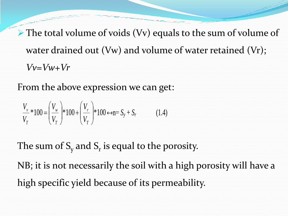
The total volume of voids (Vv) equals to the sum of volume of

water drained out (Vw) and volume of water retained (Vr);

Vv=Vw+Vr

From the above expression we can get:

The sum of Sy and Sr is equal to the porosity.

NB; it is not necessarily the soil with a high porosity will have a

high specific yield because of its permeability.

100*100*100*

T

r

T

w

T

v

V

V

V

V

V

V↔n= Sy + Sr (1.4)

4. Coefficient of permeability (k)

Coefficient of permeability (hydraulic conductivity) reflects

the combined effects of the porous medium and fluid

properties.

It is an ease with which water can flow through a soil mass or

rock and usually it is the capacity of geological formation to

transmit water.

K=ki.kw (1.5) Where: K = Coefficient of permeability, ki = Intrinsic permeability; depending on rock properties (such as grain size & packing), kW = Permeability depending on fluid properties (such as density and viscosity of water)

For unconsolidated rocks, from an analogy of laminar flow through a conduit, the coefficient of permeability K can be expressed as:

K = C dm2 ( / ) = C dm

2 (g / ) (1.6)

Where:

dm = Mean pore size of the porous medium (m),

= unit weight of the fluid (kg/m2s2),

= density of the fluid (kg/m3),

g = acceleration due to gravity (m/s2),

= dynamic viscosity of the fluid (kg/ms),

C = a shape factor which depends on the porosity, packing, shape of grains and grain-size distribution of the porous medium. Thus for a given porous material K 1/ where = kinematic viscosity = / = f (temperature).

5. Transmissivity (T) and Vertical Resistance (C):

Transmissivity is the product of horizontal coefficient of

permeability and saturated thickness of the aquifer.

For an isotropic aquifer (Kx = Ky = K):

T = KB (1.7)

Where:

T = aquifer Transmissivity (m2 / day)

B = aquifer thickness (m)

The vertical resistance of an aquitard is defined as the

ratio of the thickness of the aquitard and its permeability

in the vertical direction (kz):

C = D / KZ (1.8)

Where:

C = vertical resistance (days)

D = thickness of the aquitard (m)

There are d/t stratifications in aquifers may be stratification

with different permeability in each stratum.

Two main kinds of stratifications (flow situations in stratified

aquifers) are possible in aquifers:

a. Horizontal stratification

When the flow is parallel to the stratification as in (Fig. 1.6)

equivalent permeability Ke of the entire aquifer of thickness b =

bi is:

n

i

i

n

i

ii

e

B

BK

K

1

1 (1.9)

Transmissivity of an aquifer formation will therefore be given

as follows:

i

n

i

i

n

i

ie BKBKT

11

Figure 1.6: Flow parallel to stratification

b) Vertical Stratification

When the flow is vertical and normal to the stratification as in (Fig.1.7) the equivalent

permeability Ke of the aquifer length

n

i

iLL1

is:

n

i i

i

n

i

i

e

K

L

L

K

1

1 (1.10)

Figure 1.7 Flow normal to stratification

6. Storage Coefficient (S)

The volume of water drained from an aquifer, Vw may be

found from the following equation.

Vw=SAh

7. Specific Storage (Ss)

In a saturated porous medium that is confined b/n two

transmissive layers of rocks, water will be stored in the pores

of the medium by a combination of two phenomena;

a. water compression

b. aquifer expansion

In a unit of saturated porous matrix, the volume of water that

will be taken in to storage under a unit increase in head, or

the volume that will be released under a unit decrease in

head is called specific storage.

For confined aquifer, the relation between the specific

storage and the storage coefficient is as follows:

S = Ss*b (1.11)

Where:

S = Storage coefficient (dimensionless),

b = aquifer thickness (m)

Specific Storage is also called elastic storage coefficient and is

given by:

Ss=g (+n) (1.12)

Where:

=fluid (water) density,

g=gravitational acceleration,

=aquifer expansion,

n= porosity,

=water compressibility

Elastic storage is the only storage occurring in semi-confined

and confined aquifers

CHAPTER TWO GROUNDWATER MOVEMENT

Introduction

Figure 2.1: Subsurface water movement

2.1. Darcy’s Law

Groundwater in its natural state is invariably moving.

This movement is governed by hydraulic principles.

The flow through aquifers, can be expressed by what is known as Darcy’s

law

Darcy was a French hydraulic Engineer, investigating the flow of water

through horizontal beds of sand to be used for water filtration(1956)

The law is stated as “the flow through a porous media is proportional to

the area normal to the flow direction (A) and the head loss (hL) and

inversely proportional to the length (L) of the flow path.”

Q ~ hL and Q ~1/L and from continuity Q ~ A

And thus Q ~ hL.A/L

Figure2.2. Setup showing tube experiment of Henry Darcy

Introducing the proportionality constant K, Q = -K.hL/L.A ---

Darcy Equation

And Expressed in general terms as Q = KAdh/dl

Formulation of Darcy’s Law

The experimental verification of Darcy’s law can be performed

with water flowing at a rate Q through a cylinder of cross-

sectional area A packed with sand and having a piezometric

distance L apart(see figure below)

Fig 2.2 Pressure distribution and head loss in flow through a sand

column

Energy head, or fluid potentials, above the datum plane may be expressed by Bernoulli equation as:

Where p is the pressure

v is the velocity of flow

g is the acceleration of gravity

z is the elevation

hL is the head loss

is the specific weight of water

Subscripts refer to the points of measurement

Since the velocity of flow in porous media is very small, the

velocity head can be neglected ( v2/2g ≈0) and thus the head

loss can be obtained as:

This head loss is due to the energy loss by frictional

resistance dissipated as heat energy.

It follows that the head loss is independent of the inclination

of the cylinder

hL =

2

21

1 zp

zp

ww

Specific Discharge

Specific discharge is also called the Darcy Velocity. It is the

discharge Q per cross-section area, A. The specific discharge

is designated by q.

Form Darcy’s equation, q =

hk

AQ

Taking the limit as 0 i.e. dl

dhk

hKit

0

lim

- q =

The Darcy velocity (v) or the specific discharge (q) assumes

that flow occurs through the entire x-section of the material

without regard to solids & pores.

Actually, the flow is limited to the pore space only so that is

the average interstitial velocity

Va = nA

Q where n = porosity

actual

na

A

QQQQV

.........321

nA

QVa

*

Va > v

Validity of Darcy’s law

In general the Darcy’s law holds well for

i) Saturated & unsaturated flow

ii) Steady & unsteady flow condition

iii) Flow in aquifers and aquitard

iv) Flow in homogenous & heterogeneous media

v) Flow in isotropic & an isotropic media

vi) Flow in rocks and granular media

Darcy’s law is valid for laminar flow condition as it is governed

by the linter law.

In flow through pipes, it is the Reynolds number(R) to distinguish b/n laminar flow & turbulent flow.

For the flow in porous media, v is the Darcy velocity and D is the effective grain size (d10) of a formation/media. D10 for D is merely an approximation since measuring pore size distribution is a complex research task.

Experiments show that Darcy’s law is valid for NR < 1 and does not go beyond seriously up to NR =10.

This is the upper limit to the validity of Darcy’s laws

Fortunately, natural underground flow occurs with NR < 1.

So Darcy’s law is applicable

2.2. Hydraulic Conductivity Darcy’s law (1856), states that the rate of fluid flow (Q) through a sand sample is directly proportional to the x-sectional area of the flow (A) and the loss of hydraulic head b/n two points of measurements ( ), and it is inversely proportional to the length of the sample L. K is the proportionality constant of the law called hydraulic conductivity(the coefficient of permeability) It has the unit of velocity It describes the rate at which water can move through a

permeable medium. The density and kinematic viscosity of water must be

considered in determining the hydraulic conductivity

The general hydraulic equation of continuity of flow, which results from the principle of conservation of mass is,

From which and relating it with Darcy’s equation,

Where is the hydraulic gradient

is the head loss along the distance L

The hydraulic gradient , i is given by ,

Finally from above equation; hydraulic conductivity K can be determined as,

i = L

h (dimensionless)

v = Ki (another form of Darcy’s equation)

K = i

v

Intrinsic Permeability

It is a permeability which characterizes the ability of a porous medium to transmit a fluid.

It is dependent only on the physical properties of the porous medium: grain size, grain shape and arrangement, pore interconnections etc…

On the other hand hydraulic conductivity is dependent on the properties of both porous media and the fluid.

The r/ship b/n intrinsic permeability (Ki) and hydraulic conductivity (K) is expressed through the ff formula.

Ki = Kµ/ ρg (L2) Where µ absolute viscosity (dynamic viscosity) ρ density of fluid

Viscosity of a fluid is the property which describes its resistance to flow.

Determinations of Hydraulic Conductivity

Hydraulic conductivity in saturated zones can be determined by variety of techniques.

These include

analytical (empirical) methods,

laboratory methods,

tracer tests,

augur hole tests and

pumping tests of wells

i) Empirical formulas

Numerous investigators have studied the r/ship of hydraulic conductivity or permeability to the properties of porous media.

Most commonly used r/ship of such a formula has the ff general formula.

K = Cd2 Where C is the dimensionless constant

some specific terms of the formula is expressed as

K = fsfnd2

Where fs is the grain shape factor,

fn the porosity factor and

d is the characteristic grain diameter

ii) Laboratory Tests

In the laboratory, hydraulic conductivity is determined by permeameters in which flow is maintained through a small sample of material while measurements of flow rate and head loss are made.

A permeameter is a laboratory device used to measure the intrinsic permeability and hydraulic conductivity of a soil or rock sample.

There are two types of permeameters:

a) Constant head permeameter

b) Variable head permeameter

A) Constant head permeameters

Water enters the medium cylinder from the bottom and is collected as overflow after passing upward through the material/sample

The hydraulic conductivity is determined from the equation of Darcy as

K = VL/ (Ath)

Where L = length of sample;

t = time of measurement;

A = Area of sample;

h = head loss for the flow through the sample for a given particular test and

V = Volume of water collected through time t after passing through sample.

B) Variable(falling) head permeameter

Here water is added to the fall tube; it flows upward through the cylindrical sample and collected as an overflow.

The test in falling head permeameter consists of measuring the rate of fall of the water level in the tube and collecting volume of water overflow through time.

The flow rate in the tube is

Qtube = atube x dh/dt

Where a is the area of the tube and dh/dt is the rate of fall of head in the tube.

And the rate of flow in the sample is governed by Darcy’s law.

Thus the flow rate through the sample is

Qsample = -KiA

Where A is the area of the sample

i = h/L

From continuity equation, Qtube = Qsample

Therefore, adh/dt = -KAh/L

aLdh/h = -KAdt

Therefore, from integration,

K = aLln(h1/h2)/At

Fig. Arrangement of constant (a) and Variable (b) head permeameters

iii) Tracer tests

Field determination of hydraulic conductivity can be made by measuring the time interval for a water tracer to travel b/n two observation wells or test holes. The tracer can be a die such as sodium fluorescein or salt.

Consider the unconfined aquifer case below where the GW flow is from point A to point B.

the tracer flows through the aquifer with the average interstitial velocity, va, then;

va = Kh/(nL) Where n is the porosity, L is the distance b/n two points and h is the difference in head causing flow b/n the points. But va = L/t , Where, t is the travel time interval of tracer b/n two holes resulting

K= nL2/ht

limitations of the tracer tests are;

The holes need to be close together; otherwise, the travel time interval can excessively be long. For this requirement, the value of K is highly localized.

Unless the flow direction is accurately known, the tracer may miss the d/s hole entirely. Multiple sampling holes may help, but costly.

If the aquifer stratified with layers having different hydraulic conductivities, the first arrival of the tracer will result in conductivity considerably larger than the average for the aquifer.

iv) Auger- hole method

This method is most adaptable to shallow water table conditions.

The value of K obtained is essential for a horizontal direction in the immediate vicinity of the hole.

The value of K is given by

K = C/864 (dy/dt)

Where, dy/dt is measured rate of rise (cm/sec)

C = Constant (dimensionless),

K = hydraulic conductivity (m/day)

Fig 2.5 Diagram of an Auger hole for determining the hydraulic conductivity

v) Pumping tests of wells

The most reliable method of estimating aquifer hydraulic conductivity is the pumping test of wells.

Based on observations of water levels near pumping wells an integrated K value over sizable aquifer section can be obtained.

2.3. Aquifer flow and Transmissivity

Aquifer Flow

Aquifer flow can be one dimensional, two dimensional or more. Darcy’s equation can be used to calculate one dimensional flow in aquifers.

To obtain the volume rate of flow in aquifer, Darcy’s velocity is multiplied by cross sectional area of an aquifer normal to the flow.

Q = Av = -AKdh/dl = Aki i is the hydraulic gradient (slope of water table or piezometric surface)

Q = -WbKi

Transmissivity(T)

It is defined as the rate at which water of prevailing kinematic viscosity is transmitted through a unit width of aquifer under a unit hydraulic gradient. It follows that

T = Kb (L2/T)

Where, b is the saturated thickness of an aquifer

Therefore, the flow rate in Darcy’s equation can be given as

Q = -WbKi = Q = -WTi

The saturated thickness for confined aquifer is fairly constant and hence the value of T is constant; however, the saturated thickness for unconfined aquifers is variable as the water table varies.

Hence the Transmissivity for unconfined aquifers vary as a function of the water table variation.

Flow in anisotropic aquifers

Anisotropy is the rule where the directional properties of hydraulic conductivity exist.

In alluvial deposits this results from two conditions.

One is that the individual particles are seldom spherical so that when deposited under water they tend to rest with their flat sides down.

The second is that alluvium typically consists of layers of different materials, each possessing a unique value of K.

If the layers are horizontal, any single layer with a relatively low hydraulic conductivity causes vertical flow to be retarded, but horizontal flow can occur easily through any stratum of relatively high hydraulic conductivity.

Horizontal flow

Consider an aquifer of n horizontal layers each individually isotropic, with different thickness and hydraulic conductivity.

For horizontal flow parallel to the layers, the flow per unit width in the upper layer, q1 is given by

q1 = K1iz1 Where i is the hydraulic gradient

K1 and z1 are indicated in the figure.

Similarly, q2 = K2iz2 and the total flow qx in the horizontal direction is given by:

i for the horizontal flow is the same in each layer.

qx =

n

i

iq1

i(K1z1 + K2z2 +………….+ Knzn) (1)

If the whole aquifer system is taken as taken as homogeneous; then the total flow is:

qx = Kxi(z1 +z2+ ………+ zn) (2)

Where Kx is the horizontal hydraulic conductivity for the entire system

Equating the two equations and solving for the Kx yields:

Kx = (K1z1 + K2z2 +…………. + Knzn)/( z1 +z2+ ………+ zn)

If the thicknesses are equal, then

Kx = (K1 + K2 +…………. + Kn)/n (Arithmetic mean) Where n is the number of thicknesses.

Vertical flow

Consider an aquifer system consisting of n horizontal layers each individually isotropic, with different thickness values. If there is a vertical flow through the system, the flow q per unit horizontal area for the top layer can be expressed as: qz = K1Δh1/z1 Where Δh1 is the total head loss across the first layer Solving for Δh1, Δh1 = qzz1/K1 Similarly for the second layer and n layer: Δh2 = qzz2/K2 Δhn = qzzn/Kn The total head loss (Δht = ΔH) for vertical flow through all the layers of the system can be calculated as the sum of the head losses in each layer, Δht = ΔH = qz(z1/K1 + z2/K2+ ………+ zn/Kn) (3) In homogenous system, the vertical flow can be expressed as qz = Kz ΔH /(z1 +z2 +…..zn) and ΔH = qz (z1 +z2 +…..zn)/Kz (4) Equating the two equations (3 and 4) and solving for Kz, Kz = (z1 +z2 +…..zn) /( (z1/K1 + z2/K2+ ………+ zn/Kn) And for equal thickness; Kz = n /( (1/K1 + 1K2+ ………+ 1/Kn) (Harmonic mean)

Reading Assignment!

K-value for two dimensional flow in isotropic media

Average Hydraulic Conductivity

Groundwater flow directions

Flow nets

Flow net is a net work b/n flow lines and equipotential lines intersecting at right angles to each other.

The imaginary path which a particle of water follows in its course of seepage through a saturated soil mass is called flow line.

An equipotential line is the line which joins points with equal potential head.

Equipotential lines are lines that intersect the flow lines at right angles

flow net is constructed to quantify the flow rate through a medium.

Consider the portion of a flow net shown in figure above. The hydraulic gradient is given by:

i = -dh/ds

and the constant flow rate , b/n two adjacent lines is given by

q = -K.dm.dh/ds for unit thickness.

But for the squares of the flow net, the approximation ds ~ dm can be made.

Therefore, the above equation reduces to

q = Kdh

Reading Assignment Flow in relation to GW Contours

Groundwater Flow Directions

CHAPTER THREE WELL HYDRAULICS

Introduction

Wells are one of the most important aspects of applied hydrology.

Water wells are used for the extraction of ground water to fill domestic, municipal, industrial and irrigation needs.

Wells have also been used to:

control salt-water intrusion

remove contaminated water from an aquifer

lower the water table for the construction projects

drain farm lands and inject fluids into the ground

Basic Assumptions

The derivation of well flow equation is generally based on the following assumptions:

The well is pumped at constant rate ( Q = Constant)

The aquifer is homogenous, isotropic, horizontal and of infinite extent

Prior to pumping, the initial water level is horizontal

The aquifer is bounded on the bottom by confining layer

All changes in the position of potentiometric surface are due to the effects of pumping the well alone

All flow is radial toward the well

Ground water flow is horizontal and Darcy’s law is valid

The pumping well has an infinitesimal diameter and 100% efficient

The pumping well and observation wells are fully penetrating and they are screened over the entire thickness of the aquifer

3.1. Steady Radial Flow to a Well

Steady flow implies that no change occurs with time (the head is constant with respect to time).

3.1.1. A steady radial flow in confined aquifer

The figure 3.1 below shows a well completely penetrating a horizontal confined aquifer of thickness b.

Consider the well to be discharging a steady flow, Q

The original piezometric head is ho

The draw down due to pumping(s) is indicated below

The piezometric head at the pumping well is hw and drawdown is sw

0

t

h, Or 0

t

parameter (steady state)

Figure 3.1: Radial flow to a well penetrating confined aquifer

At a radial distance r from the well, if h is the piezometric head, the velocity of flow by Darcy’s law is:

qr = K (dh/dr)

The cylindrical surface area (A) through which this velocity occurs is 2rb.

Hence by equating the discharge entering this surface to the well discharge,

Q = Av = for steady radial flow to a well

Integrating between limits r1 and r2 with the corresponding piezometric heads being h1 and h2, respectively:

rbKdhQdr 2

2

1

2

1

2

h

h

r

r

dhbKr

drQ

)ln(

)(2

1

2

12

r

r

hhbKQ

(3.1)

If the drawdowns s1 and s2 at the observation wells are known, s1=ho-h1, s2=ho-h2 and kb=T, then equation (3.1) will be;

Further, at the edge of the zone of influence, s2=0, r2=R, h2=ho

At the well wall, r1=rw , h1=hw and s1=sw then equation (3.2) will be;

)ln(

)21(2

1

2

r

r

ssbKQ

(3.2)

3.1.2. Steady radial flow in unconfined aquifer

Consider a steady flow from a well completely penetrating an unconfined aquifer .

To obtain simple solution, depuit’s assumptions are important;

These are:

For small inclinations of the free surface, the streamlines can be assumed to be horizontal and the equipotential lines are thus vertical

The hydraulic gradient is equal to the slope of the free surface and does not vary with depth. This assumption is satisfactory in most of the flow regions except in the immediate neighborhood of the well.

Consider the well of radius, rw penetrating completely extensive unconfined horizontal aquifers as shown in Fig.3.2.

Figure 3.2: Radial flow to well penetrating an unconfined aquifer

Water is pumped out from the well at a constant discharge, Q for a long time.

According to Darcy’s law, at any radial distance r, the velocity of radial flow into the well is:

qr = K (dh/dr)

Where h is the height of the water table above the aquifer bed at that location.

For steady flow, by continuity:

Integrating between limits r1 and r2 where the water table depths are h1 and h2 respectively and on rearranging:

r

dr

K

Qhdhor

dr

dhKrhAqQ r

2,*2 ,

Eq. (3.4) is the equilibrium equation for a well in an unconfined aquifer.

At the edge of the zone of influence of radius R, H = saturated thickness of the aquifer, Eq. (3.4) can be written as:

Where:

hw = depth of water in the pumping well of radius rw

1

2

2

1

2

22

1

2

1ln

222 r

r

K

Qhh

r

dr

K

Qhdh

r

r

h

h

1

2

2

1

2

2

lnr

r

hhKQ

(3.4)

w

w

r

R

hHKQ

ln

22 (3.5)

Approximate equations: If the drawdown at the pumping well Sw = (H - hw) is small relative to H, then:

H2 - hw

2 = (H + hw)*(H - hw) 2hwSw, Noting that T = KH, Eq. (3.5) can be written as:

w

w

r

R

TSQ

ln

2 (3.6)

It is the same as Eq. (3.3) Similarly Eq. (3.4) can be written in terms of S1 = (H -h1) and S2 = (H - h2) as:

1

2

21

ln

2

r

r

SSTQ

(3.7)

3.2. Unsteady radial flow to a well

3.2.1. Unsteady radial flow in confined aquifer

Non-equilibrium well pumping equation

Where; h-head

r-radial distance from the pumped well

s-the storage coefficient

T-transmissivity

t-time since beginning of pumping

The non-steady Ground Water flow equation in two dimensions is given by:

t

h

T

S

y

h

x

h

2

2

2

2

Or in polar coordinates

t

h

T

S

r

h

r

h

2

2

Theis obtained a solution for the above eqn. based on the analog between GW flow and heat conduction.

By imposing the boundary conditions of the well as, h=ho for t=0 and h→ho as r→∞ for t≥0, the solution will be;

This equation is non-equilibrium or Theis equation

u

u

u

due is the well function defined by W(u)

B/se of the mathematical difficulties encountered in applying the above equation, several investigators developed simpler approximate solutions that can be readily applied for field purposes.

Let us deal with two of them…

a) Theis curve matching

b) Jacob approximate method

Other method is chow method…….

3.2.2. Unsteady radial flow in unconfined aquifer

3.3. Unsteady Radial flow to a well in leaky aquifers

3.4. Partially penetrating Wells

A well whose water entry is less than the aquifer it penetrates is known as a partially penetrating well.

Figure 3.4: Effects of partially penetrating well on drawdown

The draw down , swp, at the well face of partially penetrating wells in confined aquifer of transient flow can be given as:

swp = sw + Δsw

Where Δsw is additional DD due to partial penetration

The ff eqn, developed by Hantush is used for determination of draw down in a partially penetrating well;

Where: - wps is the DD of the piezometric surface by Hantush

ps is a dimensionless term = f(D/rw , Le/D)

Where D = is the aquifer thickness and Le is the open space (effective screen length)

3.5. Well Losses and Specific Capacity

Well Loss

The total DD (sw) at the well face is made up of:

i) Head loss resulting from laminar flow in the formation, sf

ii) Head loss resulting from turbulent flow in the zone close to the well face where Re > 1.

iii) Head loss through the well casing and screen

The components under (ii) and (iii) are contributing to the so called well loss.

Therefore, taking the well loss in to account, the total DD can be given as:

n

wfw

efw

QcQcs

sss

Where: - ws is the total DD at the pumping well

fs is loss in the formation due to laminar flow ( expressed by Theis)

es is the well loss ( can be observed near the pumping well)

fc is the formation loss constant.

wc is the well loss constant

n is the exponent due to turbulence

Specific Capacity

It is the ratio of discharge to drawdown in a pumping well.

It is the measure of the productivity of a well

The larger the specific capacity, the better the well is.

S. C. = Q/sw

But the value of cf can be determined from the theoretical Theis equation;

w

fr

R

T

Qs ln

2 And since sf = cfQ; cf =

T

rRc w

f2

)/ln( (if steady state flow condition

near the well is achieved)

T

SrTt

c wf

4

)25.2ln( 2

(if unsteady sate case is considered)

Therefore,

1

2

1

1

4

)25.2ln(

1/

1//

n

w

w

w

n

wf

w

n

wfw

cT

SrTt

sQ

QccsQQccQs

3.6. Multiple Well Systems

When the cone of depressions of two nearby pumping wells overlap, one well is said to interfere with another because of the increase in drawdown.

Figure 3.6: Interference of two wells in a confined aquifer

For confined aquifer, the DD at is

1

111 ln

2 R

T

Qs

For steady states of flow

2

222 ln

2 R

T

Qs

if Q1 = Q2 = ….= Qn ; rw1 = rw2 = …= rwn ; R1 = R2 = …….= Rn ;

The total DD is then given by :

sT = s1 +s2 =

1

11 ln2

R

T

Q

+

2

22 ln2

R

T

Q

for two interfering wells.

=

21

lnln2

RRT

Q

=

12

2

ln2

RT

Q

Similarly, the drawdown at any of the wells is

sw =

Lr

RT

Q

w

2

ln2

composite DD at a single well.

CHAPTER FOUR PUMPING TESTS OF WELLS

4.1 Test wells and observation wells

Test wells(pumping well): is a well where pumping is being done and observation of flow rate/discharge rate(Q) is taking place

Observation wells: a wells where observation of variation of water level (head) being under taken (also called monitoring wells)

Observation wells are located at some distances (r) from pumping well

Preliminary investigations one has to carryout before conducting pumping tests of a well:

a) The geophysical x-tics of subsurface

b) The type of aquifer and confining bed

c) The thickness and lateral extent of aquifers and confining beds

d) Boundary conditions

e) Data of ground water flow systems(horizontal, vertical), flow of groundwater , water table gradients, trends in water level

f) Data of any existing wells in the area

4.2 Performing pumping tests

Measurements in pumping well site

The following measurements can be taken in the pumping well site:

a) Water level (dynamic and static)

b) Discharge rate(Q), water quality samples

c) Duration and steps of pumping

d) Distance between the pumping and observation wells

e) Pumping position

f) Aquifer thickness

g) Set up of blind and screen casing

While locating a test well, the following points should be considered:

a) The hydrological conditions of test well should not change over short distances and should be representative of the area

b) The gradient of the water level should be low

c) The well should be located away from other recharging and discharging well

d) The well should be located away from high and heavy traffic sites where variation in head may occurs

e) The pumping water should be discharge sufficiently away from the well site

f) The site should be easily accessible for machinery, labor and construction material transport

The following points should be considered for installation and design of observation wells:

Number of observation wells

Spacing of observation wells

Length of the well screen(aquifer thickness)

Depth of observation wells

CHAPTER FIVE INTRODUCTION TO GROUNDWATER MODELLING

What is model?

Models serves as the representation of reality and its process

eg. Darcy’s law, hydrologic cycle……

From past and present conceptualizations models can be used to simulate future conditions

Models can be:-

Physical models( a scaled down system of real system)

Analog models(simulated process representing natural system, i.e hydrologic cycle)

Mathematical models( includes clear chronological sets of relations, numerical and logical steps that change numerical input to numerical output, i.e ∆s= Qin-Qout

A small object, usually built to scale, that represents in detail another, often larger object.

A schematic description of a system, theory, or phenomenon that accounts for its known or inferred properties and may be used for further study of its x-tics

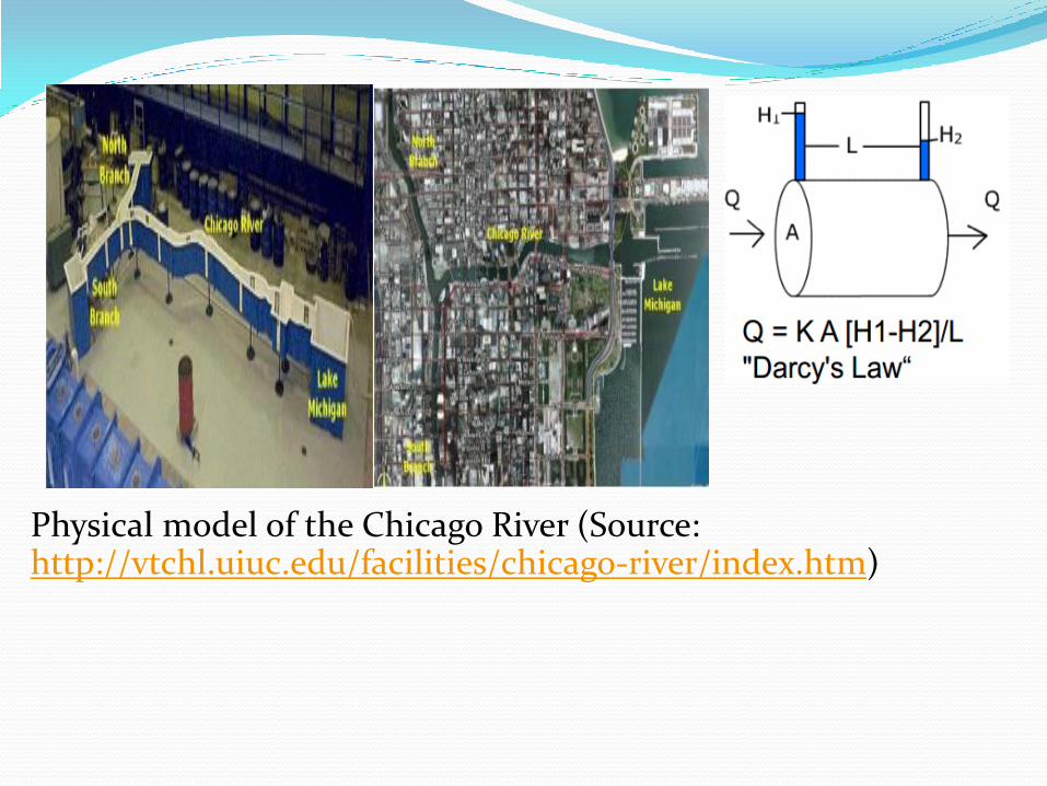
Physical model of the Chicago River (Source: http://vtchl.uiuc.edu/facilities/chicago-river/index.htm)

What models do ?

They simulate all important processes and functional r/ships within the system that they represent.

These processes are simulated by solving mathematical equations representing the system behavior and operations.

Example of computer based models

Mike-She, Mike Basin, Mike 11, HEC-1, HEC-HMS

MODFLOW, TOPMODEL,

SWAT, HBV, HYPE, ACRU, PITMAN

SWAP, ORYZA, DAIZY

WAFLEX ,WEAP, Ribasim

Others……………

Why modelling?

Modelling helps to understand system functioning

Generate knowledge and new insights about a system

Contribute to engineering design

Answer various what if questions

Support decision making process

Useful for training and education

A word of caution

Models produce information to aid decision making but not the decisions

Decision making involves:

Interdisciplinary problems

Dynamic problems

People’s wishes

Politics (consensus, time of decisions,…)

Communication with decision makers and stakeholders

Be aware that the science and facts may be ignored … !

Models are always a simplified representation of the

reality and

are based on assumptions.

Insufficient understanding

Uncertainties in measurements

Unpredictable actions of individuals or institutions

So, a modeler has to make choices when building a

model and should be well aware of the limitations

and uncertainties

Modelling protocols(procedures)

Initiating modeling project

Defining the problem to be modeled

o Impact of land use changes on hydrology

o Impact of climate change on hydrology

o Impact of construction of a dam on hydrology, water quality

o Impact of wells on groundwater flows, levels or contamination transport

Models

Simplification of reality

o Can be an scale model of the system

o Diagram of figure representing the system

o Mathematical translation

o Computer program

Model selection- structure/input-output criteria

Conceptualization of major processes

Accuracy of prediction

Simplicity of model

Consistency of parameters estimation

Sensitivity of results to changes in parameter values

Assumptions

Potential for improvement

Model selection-practical issue

o Nature of the problem

o Availability of resources and know-how

o Computing facilities

o Further applications

o Model comprehensiveness

o Model performance

o Access to data

o User friendliness

Calibration

Models are approximations of reality; they can not precisely represent natural systems

There is no single accepted statistic or test , accepted statistic or test that determines whether or not a model is valid

Both graphical comparisons and statistical tests are required in model calibration and validation

Models cannot expected to be more accurate than the errors (confidence intervals) in the input and observed data Calibration and validation

Iterative process to improve model performance

Model calibration consists of changing values of model input parameters in an attempt to match field conditions within some acceptable criteria.

Validation aims to demonstrate the ability to predict field observations for periods separate from the calibration effort.

Split- sample calibration/validation

use only a portion of the available record of observed values for calibration;

once the final parameter values are developed through calibration, simulation is performed for the remaining period of observed values and goodness-of-fit b/n recorded and simulated values is reassessed.

Simulation and presentation

Using the model

o Simulating different scenarios

o Simulating different strategies

Interpreting model results

Reporting modelling results

References

1. Brouwer, H (1978) ground water hydrology, McGraw Hill, New York

2. Driscoll, fletcher G. (1986) Ground water & wells. 2nd edition, Johnson filtration systems Inc., USA.

3. Fetter, C.W., 1980. Applied Hydrogeology, E-Merril publishing Company, New York.

4. Kresic, N (1997) quantitative solution in hydrology & ground water modeling, CRC-Press, USA

5. Kruse man, G, P & de Ridder, N, A (1994) analysis & evaluation of pumping test data 2nd

Edition, ILRI, the Netherland

6. Ragunath, H.M. (1982) Ground Water. 2ndEdition, New Age International, New Delih.

7. Todd, D.K. (1980) Ground Water Hydrology. 2nd Edition, John Wiley and Sons, California

THANK

YOU!!