STUDY GUIDE FOR A BEGINNING COURSE IN GROUND-WATER HYDROLOGY: r”- \

a ,: PART II -- INSTRUCTOR’S GUIDE

0OUNDARY D-WATER SY

U.S. GEOLOGICAL SURVEY Open-File Report 92-637

The keystone of this section and the entire course is Darcy's law, which 0 - provides the basis for quantitative analysis of ground-water flow. In this section, after establishing the necessary supporting relations, we present a simplified development of the ground-water flow equation.

Darcy3s Law

Assignments

*Study Fetter (1988), p. 75-85, 123-131; Freeze and Cherry (1979), Darcy's law--p. 15-18, 34-35, 72-73; physical content of permeability--p. 26-30; Darcy velocity and average linear velocity--p. 69-71; or Todd (1980), p. 64-74.

*Work Exercise (2-1)--Darcy's law.

*Define the following terms, using the glossary in Fetter (1988), an unabridged dictionary, or other available sources--steady state, unsteady state, transient, equilibrium, nonequilibrium.

*Study Note (2-1)--Dimensionality of a ground-water flow field.

The importance of Darcy's law to ground-water hydrology cannot be overstated; it provides the basis for quantitative analysis of ground-water flow. Several important points related to Darcy's law that are covered in Fetter (1988) are emphasized below.

(1) The physical content of hydraulic conductivity. The reason for the statement by some writers that hydraulic conductivity is a coefficient of proportionality in Darcy's experiment is demonstrated in the first part of Exercise (2-l). Theory and experiment indicate that the coefficient of hydraulic conductivity represents the combined properties of the flowing fluid (ground water) and the porous medium. The physical content of hydraulic conductivity is developed in connection with equations (4-8) and (4-9) in Fetter (1988, p. 78). The term "intrinsic permeability" designates the parameter that describes only the properties of the porous medium, irrespective of the flowing fluid, Explicit use of fluid properties and intrinsic permeability instead of hydraulic conductivity is required in analyzing density-dependent flows (for example, flow of water with variable density in fresh-ground-water/salty-ground-water problems) or flows that involve more than one phase or more than one fluid, such as flow in the unsaturated zone, in petroleum reservoirs, and in many situations that involve contaminated ground water.

28

(2) The Darcy velocity (or specific discharge) and the average linear velocity. The Darcy velocity (equation (5-24) in Fetter, 1988, p. 125) is an apparent average velocity that is derived directly from Darcy's law. The average linear velocity (equation (5-25) in Fetter, 1988, p. 126), the Darcy velocity divided by the porosity (n), is an approximation of the actual average velocity of flow in the openings within the solid earth material. In m>st practical problems, particularly those involving movement of contaminants, the average linear velocity is applicable.

(3) Dimensionality of flow fields. Flow patterns in real ground-water systems are inherently three-dimensional. Hydrologists commonly analyze ground-water flow patterns in two or even one dimension. The purpose of Note (2-l) is to introduce the concept of flow-system dimensionality. The hydrologist must differentiate between the ground-water flow patterns found in a real ground-water system and what is assumed about these flow patterns as an approximation in order to simplify their quantitative analysis.

Comments

Freeze and Cherry (1979, table 2.3, p. 29) provide a useful conversion table, not only for units of,hydraulic conductivity (K) [LT"] and intrinsic permeability (k) EL*], but also for conversion of hydraulic conductivity to intrinsic permeability and the reverse. Both Freeze and Cherry (1979) and Fetter (1988) discuss the relation

PS K=k--,

Ir

where p is the mass density of the flowing fluid [ML"], g is the acceleration of gravity [LT'*], and /A is the absolute viscosity of the flowing fluid [ML-'T-l]. To convert back and forth between K and k (see formula above), a

PS value for -? ( 1 water is required. The precise value of this composite

P conversion factor depends on temperature because pwater is slightly temperature-dependent and pwater is highly temperature-dependent. An example problem for this conversion is given by Fetter (1988, p. 84).

The discussion in Freeze and Cherry (1979, p. 69-71) on ground-water velocity is the most lucid that we have seen.

29

Answers to Exercise (S-l)--Darcy's law a .. Table 8-l .--Data from hypothetical experiments with the laboratory seepage

system

[Q is steady flow through sand prism; Ah is head difference between two piezometers; 1 is distance between tw piezometers; A is constant cross-sectional area of sand prism (fig. 2-l)]

Test number

Q (cubic feet per day)

Ah (feet) Ah/ 1

Q/A (feet per

day)

1 2.2 0.11 0.0275 1.82

2 3.3 .17 .0425 2.73

3 4.6 .23 .0575 3.80

4 5.4 .26 .065 4.46

5 6.7 .34 .085 5.54

6 7.3 .38 .095 6.03

7 7.9 .40 . 100 6.53

30

Awwcrs to Exercise (S-l) (continued)-- (I), (a), (3)

107 : -... :..i..i.. -:..:.:..I.. . . . * d*“>.!..:‘. --;..;.;..:.. . . 1 .

: : : : -. . . +. . 2 . . . . . . . b.. . . . :. .:. . . . . . -2-e..a-.*.. . . * .

. . . . . . . . . . . . . . . . . .

-j-.:.-i-.,. A..:.:..“. . . . . ..<..?.!..:‘. --:..;.;..:.. * . . .

.r..;.;.;.. +..;.;..

.,.. ‘..:.A. . . . . :.:..E.. .*.. . . . .

.<..>.:..p. .<..~.~..~.

.;..;.;.;.. .;..;.;.;. . . . . . . . .

. . ..+.+ m;..;. . +.:.a .: . . . . . . A. .:..:.:..z..

T

. . . .a . . . ..m. :.. . . . . . . . . . . a..... ::: -*** .3 ..,.,..... m;..;.:..:.. . . . . . . . .

. . . . .-:--:-.;-.!- .;..~..i.-:..

. . . . . . ..:.A. .: .-.. z-2.. . . . . ..*. .<..>.:..>. .<..>.:..:‘. .;..;.;..:.. .;..;.;.;* .*.. *...

. . . . . ..+..‘..i.. ..;..:.. j..:.. .L . . . . :.,. .:..,.:.,.

> . j . .f . . ‘-. f . j . .I

,.... :.:..,. .,....:..:. . ..a . . . .

.‘-.>-:..2. .<..:.<.m>

.;..;.;..:.. .;..;.;.:. . . . . . . . .

: : : : ‘..* -... . .*..... I .;..:-.i..:. . . . . . . . . :..,. .:..:.:..: . . . . . . . .

MOC EL THROUGHFLOV

MODEL ( ROSS-SECTIONAL

..~..~.i..;.. ..:..;.;..:m

.A.‘.:..‘. .:..:.:..:. . . . . . ..*

1

.3.>.‘..>. .a . . . . :..:-

.;.;.i..:.. .;..;.;.:. . . . . . . . . . . . . . . . .

..:..>.j..;.. ..;..>.j..:.

.:..:.:..:. .:..:.:..:. . ..I . . .

--I-

“.“:‘:.-“. .a . . . . . t..:.

.;..;.;..:.. .:..:.;..t . . . . . . . .

. . . . . . . . --:--i-j.-:-. -i--S-i--:.

. . . . ..*. ,...-. . . . . . . . . . . . . . . . . . . . . . . . -.;..>.a..%.

: : .< . . . . !..

.;..; .,..... .; ..,.; .:. ..*. . . .

. ..* . . . . .i..:.:..>. .$..>.!W.‘-. .;..;-;.-:.. .;..;-;..:.. . . . . . . . . . ..:..:+~.. . . . . . . . . . . . i-2. .&.-i..‘. .:..: -... ‘. . . . . . . . . .<..:.+..:.. .,*.- :.i..‘.-. .;..;.;..:.. .;..;-;..:.. . . . . . . . . . . . ..I +.j..‘. ..:..>.j..:.. ‘(4.b,‘6:2 i iO-‘,:

.*: .‘:: .;..;.; . . ..- .;..; .,..... . . . . ..a. . ..* . . . .

. .:..I. j-.:. . . .:..:. . j..f . . . . . . . . . . :..... .,..1.:..,. . . . . . ..* .<..>.f..?. .,..:.a...>.

,.;..;.;..:.. .*..;.;..:.. . . . . . . . . . . . .:..:-. i..:. .

.<.A . . . . z.. .+;..;. .-.. :.:..,. . . . . . ..a -<‘.:.f..?. .<..~.~..~.

.;..;-;..;. .;..;.:..;. . . . . .,.* . . . . * .

.j..>.<..>. .,..;.j+. * . e..... :..,. .:..:.:.A.. ..a .,.. .a*..?.!..;.. ..y.!..>.

..I..;.;..:.. . . . . ;.;..:.. . . . . . . . .

.-.-....i--... e;e-;-j.o:.m : : * : . .

(Q) AREA (A)’ IN FEE-

PER DAY

. . *. .E . j . 1. . i I ..:..;.;..;.. ..:. . . .:..: .... :

..;. .A.:...‘. .:..:.:..z.. .:..:.:..z.. ... .$ ..: .f .. { ... .... .. .;..;.;.;.

.y.>.+ .:‘.:.:..c.

.... ;.;.; .. .<..;.;..;. ............

.... +. .j..: ..... .;..;.j..: .. ..;..;.j..: .... . ... :.:. .:..:.:.;. .:..:.:..:. ... .:..>.:..; .. ..... ..*..:.:.$. .a*..: ............ -;..;.;..: . . .;..:.;.; .. .&4.; .... ............

.... ..:..:..i..: ..~..;.j..:

.. .. .. ~~~-~~~i-~:.~

.-‘..:.:..I.. ..:..:.:..z.. .A.:.:..‘. .......

.<..>.!..>. .<..>.& ....

.. .a...:.<..‘-. .;..;.;..: .. .;.....; ....... ..... . .;..;.;..;. ....

Figwe 8-8. --Plot of data from hypothetical eaqxriments with the laboratory seepage system illustrating a linear relation between hydraulic gradient (Ah/l) and model throughf low (8). area (A) is constant .)

(Model cross-sectional

31

Answers to Exercise (a-1) (continued)

(1) A "good" straight-line or linear relation (fig. 2-2).

(2) y = mx + b is a standard formula for a straight line, where m is the slope of the line and b Is the y-intercept.

Substituting parameters from figure (2-2),

Ah Q -- cm - +b 1 A

Ah Q however, when -- = 0, - = 0 and b = 0.

1 A

Thus, from our knowledge of the physical experiment, we know that the experimental line must pass through the origin. As a result, our experimental line can be represented by

Y = mx, or

Ah Q -- =m - . 1 A

(3) Ym -Y1 m I -----.

xn -X1 6.2 x 10" - 0 6.2 x 1O-9

See graph on figure (2-2); m = -------------- = ---------- = 1.55 x 10-r. 4.0 - 0 4.0

1 Ah

(4) Q = - A i- l m

1 1 (5) Numerical value of K = - = ----------- = 64.5 ft/d.

m 1.55 x 10"

(6) See figure (2-l).

32

Exercise (8-l) -- (6) (continued)

,WATER LEVEL / VALVE

A

.

!3fi

QN . . ‘.‘_ ,‘,’ . ,’ CROSS-SECTIONAL AREAL;

OF SQUARE SAND PRISM = 1.1 FEET X 1.1 FEET =

1.21 FEET SQUARED

.

/PIEZOMETER

FLOWLINES

k: &= 4 FEET

’ IN = Q,,, (CUBIC FEET PER DAY)

THIS STEADY FLOW EQUALS THE OVERFLOW FROM THE

CONSTANT -HEAD TANK, WHICH IS MEASURED HERE

v \, B

CONSTANT- HEAD TANK

‘OTENTIAL LINES I

AC = UPSTREAM END OF PRISM OR INFLOW SURFACE = CONSTANT- HEAD BOUNDARY

BD = DOWNSTREAM END OF PRISM OR OUTFLOW SURFACE = CONSTANT- HEAD BOUNDARY

IN THREE DIMENSIONS THE WALLS OF THE DARCY PRISM ARE IMPERMEABLE, THAT IS, NO-FLOW OR STREAM-SURFACE BOUNDARIES. THUS, AB AND CD ARE NO-FLOW BOUNDARIES

Figure B-1. --Sketch of laboratory seepage system showing boundary conditions of sand prism and representative flowlines and potential lines within sand prism.

33

Exercise (%1)--(7)(a) (continued)

(7)(a) From Fetter (1988), problem 6, p. 159

A confined aquifer is 10 ft thick. The potentiometric surface drops 0.54 ft between two wells that are 792 ft apart. The hydraulic conductivity is 21 ftld and the effective porosity is 0.17.

(a) How much water, in cubic feet per day, is moving through a strip of the aquifer that is 10 ft wide?

(b) What is the average linear velocity?

Thickness of confined aquifer = 10 ft

Distance between wells = 792 ft

Change in head = 0.54 ft

Hydraulic conductivity = 21 ft/d

Effective porosity = 0.17

NOT TO SCALE

Sketch of problem 6 in Fetter (1988), p. 159.

Solution Q dh

(a) Using v = - = -K -- (equation 5-24, Fetter (1988, p. 125)) and A dl

dh 10 ft l 10 ft l 2lft/d l 0.54 ft rearranging Q = M _- = ___-___--__--_------------------ = 1.432 fta/d

dl 792 ft

Q -K dh (b) Using V, = --- = ------ (equation 5-25A, Fetter (1988, p. 126)),

neA ne dl

1.432 fta/d Vx ~5 ------------_- = 0.084 ft/d, or

0.17 l 100 fta

21 ft/d l 0.54 ft V, = ------------__--m. = 0.084 ft/d

0.17 l 792 ft

Note: Average linear velocity is commonly designated 7.

34

Exercise (S-1) -- (7) (6) (cant inued)

(7)(b)--From Fetter (1988), problem 7, p. 160

A constant-head permeameter has a cross-sectional area of 156 cn?. The sample is 18 cm long. At a head of 5 cm, the permeameter discharges 50 cn? in 193 5. What is the hydraulic conductivity in

(a) cm/s?

(b) ftld?

Cross-sectional area of sample= 156 cn?

Sample length = 18 cm

I I NOT TO SCALE

Sketch for problem 7 in Fetter (1988), p. 160.

Solution

VL (a) Using K = --- (equation 5-26, Fetter (1988, p. 128))

Ath

(50 cti) (18 cm) R= --__--------------------

(156 cd) (193 s) (5 cm)

K= 5.98 x 10'8 cm/s

(b) (5.98 x 10" cm/s) x 86,400 s/d x ft130.48 cm = 16.95 ft/d

35

Transmissivity

Assignments

*Study Fetter (1988), p. 105, 108-111; Freeze and Cherry (1979), p* 30-34, 59-62; or Todd (1980), p. 69, 78-81.

*Work Exercise (2-2)--Transmissivity and equivalent vertical hydraulic conductivity in a layered sequence.

Transmissivity is a convenient composite variable that applies only to horizontal or nearly horizontal hydrogeologic units. In order to analyze vertical ground-water flow, we must use values of hydraulic conductivity that are appropriate to the vertical direction. Exercise (2-2) provides practice in the use of equations (4-16), (4-17), (4-22), and (4-23) in Fetter (1988, p. 105, 110).

36

Answers to EZercisc (I%$?) --Transmissivity and Equivalent Vertical Hydraulic Conductivity in a Layered Sequence

(1) Use equation (4-17), p. 105, and equation (4-22), p. 110, in Fetter (1988).

Bed Bed thickness number (feet)

Bed hydraulic conductivity (K) Bed transmfssivity (T)

(feet per day) (feet squared per day)

1 25 10 250

2 30 100 3,000

3 20 .OOl .020

4 50 50 2,500

5,750 fta/d = T

d = 25 + 30 + 20 + 50 = 125 ft (total thickness of sequence)

T 5,750 (Equivalent) K(x,y) = ; = -;;;- = 46 ft/d

(2) Use equation (4-23), in Fetter (1988, p. 111). A derivation of this equation can be found in Freeze and Cherry (1979, p. 32-34).

125 125 (Equivalent) K, = --------------e----- = -w---- = 0.00625 ft/d

25 30 20 50 20,000 -- + --- + --- + -- 10 100 .OOl 50

(Denominator) 2.5 + .3 + 20,000 + 1 t 20,003.8

(3) In general, the most permeable beds exert the greatest influence on the transmissivity, and the least permeable beds exert the greatest influence on the equivalent vertical hydraulic conductivity.

Note that in this problem we assume that each individual bed is isotropic and homogeneous with respect to hydraulic conductivity. In a more realistic problem, we would use different values of Kx and K, for each bed.

37

Aquifers, Confining Layers, Unconfined and Confined Flow

Assignment

*Study Fetter (1988), p. 101-105; Freezeaand Cherry (1979), p. 47-49; or Todd (1980), p. 25-26, 37-45.

The physical mechanisms by which ground-water storage in saturated aquifers or parts of aquifers is increased or decreased (described in the next section) are determined by the hydraulic conditions under which the ground water occurs. In nature, ground water in the saturated zone is found in unconfined aquifers and confined aquifers. The approximate upper bounding surface of the saturated zone is the water table, which is overlain by the unsaturated zone and is subject to atmospheric pressure, whereas confined aquifers are overlain and underlain by confining units. A confining unit has a low hydraulic conductivity compared to that of the adjacent aquifer. Ratios of hydraulic conductivity generally are at least 1,000 (aquifer) to 1 (confining unit), and commonly are much larger. In addition, the head at the top of the confined aquifer always is higher than the altitude of the bottom of the overlying confining unit. This means that the entire thickness of the confined aquifer is fully saturated.

Reference

Lohman (1972b), p. 2, 5, 7 (refer to aquifer; artesian; confining bed; ground water, confined; ground water, unconfined).

38

Ground-Water Storage

Assignments

*Study Fetter (1988), p. 73-76, 105-107; Freeze and Cherry (1979), p. 51-62; or Todd (1980), p. 36-37, 45-46.

*Study Note (2-2)--Ground-water storage.

*Work Exercise (2-3)--Specific yield.

Hydraulic parameters for earth materials can be divided into (1) transmitting parameters and (2) storage parameters. We already have encountered the principal transmitting parameters --hydraulic conductivity (K) or intrinsic permeability (k), and transmissivity (T). In this section the principal storage parameters and specific yield (Sy)--are

--storage coefficient (S), specific storage (Ss), introduced.

The physical mechanisms involved in unconfined storage are different from those involved in confined storage. A change in storage in an unconfined aquifer involves a physical dewatering of the earth materials; that is, earth materials that previously were saturated become unsaturated. When a change in storage takes place in a confined aquifer, the earth materials in the confined aquifer remain saturated.

Reference

Lohman (1972b), p. 12, 13 (refer to specific retention; specific yield; storage, specific; storage coefficient).

Comments

The treatment of aquifer and water compressibility and effective stress in Freeze and Cherry (1979, p. 51-58) is too detailed for presentation in this course, but it provides the necessary background for any level of discussion on storage in confined aquifers that the instructor chooses to undertake. Key concepts are the fundamentally different physical mechanisms controlling changes in storage in unconfined and confined aquifers and the related large differences in storage coefficients between these two aquifer types.

39

Answers to Exercise (2-S) --Specif ic Yie Id

A rectangular prism whose base is a square with sides equal to 1.5 ft and height equal to 6 ft is filled with fine sand whose pores are saturated with water. The porosity (n) of the sand equals 34 percent. The prism is drained by opening a drainage hole in the bottom and 2.43 fta of water is collected. Calculate the following quantities:

total volume of prism 1.5 ft x 1.5 ft x 6 ft = 13.5 fts

volume of sand grains in prism .66 x 13.5 = 8.91 fta

total volume of water in prism before drainage .34 x 13.5 = 4.59 ftr

volume of water drained by gravity 2.43 ftg

volume of water retained in prism (not drained by gravity)

4.59 - 2.43 = 2.16 fta

specific yield 2.43113.5 = .18

specific retention 2.16/13.5 = .16

0.34 By definition, specific yield + specific retention = porosity (n).

40

(1) Assuming the value of specific yield determined above, what volume of water, in cubic feet, is lost from ground-water storage per square mile for an average 1-ft decline in the water table?

VW = SAAh (equation (4-21), Fetter (1988, p. 107))

VW = .18 x 5,280 ft x 5,280 ft x 1 ft = 5,018,112 fta

Express this volume as a rate for 1 day in cubic feet per second.

5,018,112 ft8 -..------------ = 58.08 ft?/s

86,400 s

Express this volume as depth of water in inches over the mi2.

.18 x 12 in. = 2.16 in.

(2) Assuming the value of specific yield determined above, a volume of water added as recharge at the water table that is equal to (a) 1 in. and (b) 4.8 in. per unit area would represent what average change in ground-water levels, expressed in feet?

VW = SAAh

SA ft

(a) 1 ft2 x 1 in. x ------ 12 in.

Ah = ----------_--__-___--- = .463 ft . 18 x 1 ft2

ft (b) 1 ft' x 4.8 in. x ----em

12 In. Ah = ------------------------- St 2.22 ft

. 18 x 1 fta

41

Ground-Water Flow Equation

Assignments

*Study Fetter (1988), p. 131-136; Freeze and Cherry (1979), p. 63-66, 174-178, 531-533; or Todd (1980), p. 99-101.

*Study Note (2-3)--Ground-water flow equation.

*Define the following terms by referring to any available mathematics text that covers differential equations--independent variable, dependent variable, order, degree, linear, nonlinear.

A differential equation that describes or "governs" ground-water flow under a particular set of physical circumstances can be regarded as a kind of mathematical model. In ground-water flow equations, head generally is the dependent variable. If the flow equation is solved, either analytically or numerically, values of head can be calculated as a function of position in space in the ground-water reservoir (coordinates x, y, and z) and time (t). The differential equatfion provides a general rule that describes how head must vary in the neighborhood of any and all points within the flow domain (ground- water flow system). Numerical algorithms that are amenable to solution by digital computers (for example, the finite-difference approximation of a differential equation) can be developed directly from the differential equation.

The ground-water flow equation developed in Note (2-3) is widely applicable. Note that the steady-state form of this equation represents the mathematical combination of (1) the equation of continuity and (2) Darcy's law.

Comments

Many students with weak backgrounds in mathematics "tune out" whenever they see a derivative, not to mention a differential equation. The role of the instructor in discussing Note (2-3) on the ground-water flow equation is to help the participants interpret the mathematical notation and continue beyond it to the underlying physical concepts in the derivation, which were introduced previously in this course. The mathematical notation can be regarded as a powerful "shorthand" language for expressing physical relations.

As a follow-up to the idea that a differential equation used to describe a ground-water system or problem contains important physical information on an investigator's assumptions about that system or problem, participants will benefit greatly from discussion of and practice in what can be termed "differential-equation recognition." Specifically, participants will benefit from learning to identify in the differential equation features such as (1) *dependent and independent variables; (2) dimensionality of flow system (one-, two-, or three-dimensional); (3) steady versus unsteady flow; (4) identification of parameters (hydraulic conductivity (K), transmissivity (T), storage coefficient (S), specific storage (S,), aquifer thickness (b or m), and area1 recharge (W)); and (5) the presence or absence and the position of the conductive parameter (K or T) in the equation, which indicates the

42

assumptions of the investigator concerning the properties of the earth material in the system under study--for example, the earth material is isotropic and homogeneous, anisotropic and homogeneous, or anisotropic and heterogeneous. In reports on ground-water studies, the ground-water-flow equation that is used in the quantitative analysis usually is written in only four or five different ways , not including possible minor variations. Several of these ways are simplifications of the flow equation derived in Note (2-3). Examples of often-used equations and their corresponding assumptions follow.

(1) 6'h 6ah --- + --- = 0 8x2 6i9

(h is dependent variable, x and z are independent variables; two dimensions; steady flow; flow medium is isotropic and homogeneous; flow domain is a vertical section)

Ph Ph (2) K, --- + K, --- = 0

8x2 69

(same as (1) except medium is anisotropic and homogeneous)

t3) %; (Kx ;;) + %; (Kz !) = o

(same as (1) except medium is anisotropic and heterogeneous)

(dependent variable h, independent variables x, y, t; two dimensions; unsteady flow; T varies in x and y directions; flow is horizontal, or nearly so)

43

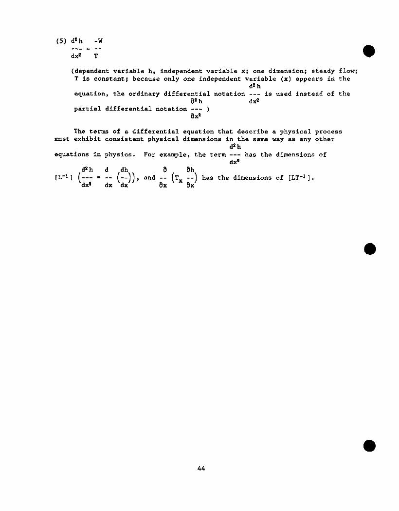
(5) d*h -W --- = -- dxg T

(dependent variable h, independent variable x; one dimension; steady flow; T is constant; because only one independent variable (x) appears in the

d2h equation, the ordinary differential notation --- is used instead of the

@h dx2 partial differential notation --- )

6X2

The terms of a differential equation that describe a physical process must exhibit

equations in

d2h [L-l] (;;; =

consistent physical dimensions in the same way as any other d2h

physics. For example, the term --- has the dimensions of dx'

d dh -- --

( 1) , and ,p (TX %q, has the dimensions of [LT'I]. dx dx

SECTION (3)--DESCRIPTION AND ANALYSIS OF GROUND-WATER SYSTEMS

The first three subsections below--system concept, information required to describe a ground-water system, and preliminary conceptualization of a ground-water system--introduce the system concept as it is applied to ground- water systems. The system concept is exceedingly useful in ground-water hydrology. It provides an organized and technically sound framework for thinking about and executing any type of ground-water investigation and is the basis for numerical simulation of ground-water systems, the most powerful investigative tool that is available. Although the system concept usually is not developed in a beginning course in ground-water hydrology to the extent that it is here, its fundamental importance , particularly as a framework for :hinking about a ground-water problem, warrants this emphasis.

An example of the need for "system thinking" in practical problems is the "site" investigations of ground-water contamination from point sources, a major activity of hydrogeologists at this time. Many of these studies suffer irreparably from the investigators' failure to apply "system thinking" by not placing and studying the local "site" in the context of the larger ground-water system of which the "site" is only a small part.

System Concept

0 Assignment

*Study Note (3-1)--System concept as applied to ground-water systems.

In Note (3-l), attend particularly to the list of features that characterize a ground-water system. Although these features may seem to be abstract at this time, the reasons for this formulation will become evident as we proceed.

Reference

Domenico (1972), p. 1-21.

Comments

From the standpoint of this course, the content of Note (3-l), although brief, is designed to be self-contained. A much broader perspective on the system concept is provided by Domenico (1972, p. 1-21).

45

Information Required to Describe a Ground-Water System

Assignments

*Study Fetter (1988), p. 533-534; or Freeze and Cherry (1979), p. 67-69, 534-535.

*Study Note (3-2) --Information necessary to describe a ground-water system.

In these and other study assignments, concentrate particularly on all the available information about the boundary conditions used in ground-water hydrology (name, properties, and physical occurrence in real ground-water systems). This is the most important new information in this section and also the most difficult to apply to specific problems.

Reference

Franke, Reilly, and Bennett (1987), p. l-10, 14-15.

Comments

The discussion in Note (3-2) on the information necessary to describe a ground-water system can begin profitably with a patient review of table (3-l). With the help of the class, make a list of the common natural and human stresses on ground-water systems.

Because we routinely measure heads in the field, we are most aware of and, thus, regard changes in head as the principal response to stress in ground-water systems. Our best opportunity to measure changes in ground-water flow in response to stress is to monitor changes in base flow of streams. Unfortunately, interpretable base flow data commonly are not available for this purpose unless a special program of data collection is established--for example, a systematic series of periodic base-flow measurements.

Among the pertinent features of a ground-water system listed in table (3-l) of Note (3-2), beginning hydrologists have the greatest conceptual difficulty with boundary conditions. Adequate information on boundary conditions for this course is provided by Franke and others (1987). Distinguishing between physical boundary conditions--that is, a description of actual hydraulic conditions at the boundaries of the ground-water system in the field--and mathematical boundary conditions, which usually are a highly idealized and simplified representation of these conditions, is essential for an overall understanding of boundary conditions by participants. In fact, at this juncture in the course, the discussion of physical boundary conditions is as important as the discussion of mathematical boundary conditions. For example, ground-water recharge to the water table is intermittent and highly variable in space and time, both during the annual hydrologic cycle of a given year and from year to year. However, we often treat area1 recharge as a constant-flux boundary in analytical solutions and numerical simulations--that is, estimates of actual recharge are averaged for a period of years, and this average flux is applied to a model of the natural ground-water system.

We recommend that instructors review all aspects of boundary conditions at every opportunity during the rest of this course , particularly in relation to concrete examples.

46

Preliminary Conceptualization of a Ground-Water System

Assignments

*Study Note (S-3)--Preliminary conceptualization of a ground-water system.

*Work Exercise (3-1)--Refining the conceptualization of a ground-water flow system from head maps and hydrogeologic sections.

*Refer to figure l-7 of Note (l-l) on head, in which three pairs of observation wells are depicted, each pair illustrating a different relation between shallow heads and deeper heads. On the basis of your study of the ground-water system in Exercise (3-l), where would you expect to find each pair of observation wells in a "typical" ground-water system, irrespective of the scale of that system?

After finishing the assignments, note that (1) our conceptualization of a ground-water system is based on what we know about that system at any particular time and must be revised continually as new information becomes available; and (2) a system conceptualization that bears little resemblance to the real system under study may lead to quantitative analyses of that system that are grossly in error because, in essence, the "wrong" system is being analyzed.

Reference

Freeze and Cherry (1979), p. 193-203.

Comments

Table 3-l in Note (3-2) on information necessary for definition of a ground-water system and table 3-2 in Note (3-3) with steps for developing a conceptual model of a ground-water system provide a general, although somewhat abstract, framework for thinking about a ground-water system or problem. Applying this general, conceptual framework to a specific ground-water system requires practice and a general knowledge of ground-water hydrology. We must expect that most course participants will be lacking in both prerequisites. The first ground-water system to be studied in considerable detail in this course is described and analyzed in Exercise (3-l). We reconanend that the two tables referred to above be used as guides and referred to explicitly in all discussions by the instructor on this ground-water system so that participants will learn what the information in the tables means through application to a concrete example.

Exercise (3-l) consists of three parts: (1) analysis of the unstressed system (questions 1 to 5), (2) analysis of the system stressed by a pumped well (question 6), and (3) analysis of a system that is similar to that in parts (1) and (2) except that the confining layer is discontinuous rather than continuous. We recommend that at least parts (1) and (2) be completed during the course.

47

Answers to Exercise ($-1)--Refining the Conceptualization of a G+round-Water Flow System from Head Maps and Hydrogeologic Sections

The purpose of this exercise is to demonstrate (1) how the three- dimensional distribution of hydraulic head in a ground-water system can be depicted accurately on a series of maps and sections derived from (a) pertinent hydrologic data, (b) knowledge of the physics of ground-water flow, and (c) a preliminary conceptualization of the structure and operation of a ground-water system; and (2) how this depiction of the head distribution either is a con- firmation of our initial conceptualization of the system or includes a modifi- cation of our initial conceptualization. The modification process is based on the results of the mapping analysis and the data utilized, and indicates an evolution in our level of understanding of the ground-water system. Inherent in item 2 is the implication that the complete integration of available hydrologic data, knowledge of physics, and hydrologic experience in the mapping analysis can improve our understanding of a ground-water flow system.

This mapping exercise is a qualitative analysis of the available data and undoubtedly is subject to some subjectivity and the professional judgment of the hydrologist making the analysis. Nonetheless, as we point out throughout the exercise, the knowledge and experience of the hydrologist must be incorporated into the final conceptualization of the ground-water system so that it represents a complete integration of the three factors listed above.

Head maps commonly are used to interpret the behavior of ground-water systems. Head maps are used to evaluate the direction and rate of ground- water flow within an aquifer; Head maps of layered aquifers commonly are used to estimate zones of upward and downward flow between the aquifers. Head maps for different hydrologic conditions can be compared to evaluate the response character of a ground-water system. The accuracy of such interpretations depends on the degree to which an understanding of the operation of the ground-water system is incorporated in the mapping exercise.

Perhaps the most demanding application of head maps and sections is their use in the calibration of ground-water-flow-simulation models. In this case, a model's ability to represent the structure and operation of a ground-water flow system is assessed largely on the basis of its ability to reproduce the three-dimensional distribution of hydraulic head in the system as depicted by maps and sections of observed head. The model integrates the physical laws that govern ground-water flow with the charatiteristics of the ground-water system--its boundary conditions, its hydrogeologic framawrk (geouwtry), the distribution of water-transmitting properties, and the presence of any internal ground-water sources or sinks. Head maps that are constructed without consideration of these factors are not an accurate representation of the flow system and are not a suitable gage with which to evaluate the validity of a ground-water model.

48

The mapping exercise consists of three parts. The first part "Mapping hydraulic head in a layered ground-water system," presents the mapping problem as a sequence of steps. It begins with mappIng the water table, continues with mapping the potentiometric surface in the confined aquifer, and ends with mapping the hydraulic head in selected sections. The instructions repeatedly suggest the advisability of returning to maps already drawn and modifying these maps on the basis of the information gained from subsequent maps or sections and the associated data. This stepped approach is used in this part of the exercise to reinforce two important considerations:

(1) The head map and section sets represent a complete picture of hydraulic head in the ground-water system and, therefore, should be constructed concurrently; and

(2) even sparse head data for an aquifer can be used to define the head surface in the aquifer when considered together with head data for overlying or underlying aquifers.

The final product of the set of head maps and sections is a depiction of the three-dimensional distribution of hydraulic head in the ground-water system. To reinforce this fact, the instructor should point out that contour

.lines, which conventionally are considered to be a linear expression on a two- dimensional surface, are in reality contour surfaces through three-dimensional space. A contour line is the expression of that three-dimensional three- dimensional surface in the plane of the map or section. An understanding of the three-dimensional nature of ground-water systems, in terms of their framework, boundaries, water-transmitting properties, head distributions, flow

0 patterns, and related heterogeneities, is arguably the most critical factor in achieving an understanding of the structure and operation of a ground-water system.

The second part of the exercise, "Mapping hydraulic head in a layered ground-water system with a pumped well," is designed to demonstrate the added understanding of a ground-water system that is gained from analyzing and comparing hydraulic heads under stressed and unstressed conditions. The third part of the exercise, "Mapping hydraulic head in a layered ground-water system with a discontinuous confining unit," presents a case in which the observed- hydraulic-head data are inconsistent with our original conceptualization of the ground-water system and which involves reformulation or refinement of our flow-system concept as part of the mapping exercise.

The following sections provide detailed solutions to all three parts of the head-mapping exercise. This exercise provides an opportunity that is not available in field investigations of ground-water systems--that is, the opportunity to compare the student's interpretation of sparse hydrologic data to an exact solution of the head distribution within the system. The hypothetical ground-water systems presented in this exercise were represented exactly in a numerical ground-water-flow-simulation model. The locations of observation wells were established at model nodes, head data for each synoptic measurement were taken from specific steady-state-model simulation results, and the answer map and sections were constructed from complete simulation results. Thus, the system concept presented and suggested for use in constructing the head maps and sections is virtually an exact replica of the system under study, whereas results of field investigations never replicate the real system exactly.

49

In field investigations of ground-water system8 , no exact solutions exist. Conceptual models are never exact, but are crude and grossly simplified approx imations of the real system. These simplifications are found in both system

d

detail and hydrologic condition. Features of system detail that can never be defined fully in our conceptual model include details of boundary representa- tion, hydrogeologic framework, and variations in water-transmitting properties that are present at a finer scale than can be measured and mapped with avail- able data. Simplifications of hydrologic condition involve the assumption that the observed data approximate a steady-flow condition within the aquifer system. Synoptic head measurements undoubtedly are affected to some degree by the dynamic nature of ground-water systems, and express the effects of seasonal fluctuations, longer-term climatic trends, or variations in pumping rates. Consideration of such complexities in mapping head in actual field investiga- tions is virtually impossible but adequate design of monitoring programs can minimize their effect. An adequate monitoring network can provide indirect information about the scale of heterogeneities that is relevant to the objectives of the analysis. Synoptic measurements can be scheduled to provide a picture (measure) of the hydrologic system that is consistent with the hydrologic condition being analyzed.

The remainder of this discussion consists of detailed answers to specific questions in Exercise (3-l).

Question 1 .--Boundary condition8 must be represented over the entire external boundary surface of the ground-water flow system. The maps and sections in figure 3-2 provide a three-dimensional picture of the system and its boundary surface. The boundary conditions on the boundary surface are as follows: The contact between the aquifer system and bedrock is assumed to be a no-flow, or streamline, boundary; the water table is assumed to be a free-surface and a constant-flux boundary, where recharge from precipitation enters at a constant rate and the water-table surface can move in response to change8 in hydrologic conditions; the surface ofdcontact between the aquifer system and the surface water in the lake (lake bottom) is assumed to be at a constant head that is equal to the stage of the lake; the contact between the aquifer system and the streambed is assumed to be a head-dependent-flux boundary, where the ground-water discharge to the stream is controlled by (1) the difference in head between the stream stage and the head in the surrounding aquifer, and (2) the hydraulic properties of the streambed and adjacent aquifer material.

Mapping hydraulic head in a layered ground-water system

6jM3tiOBS 8 t0 b.--Questions 2, 3, and 4 relate to mapping hydraulic head in the unconfined aquifer, in the confined aquifer, and on two sections, respectively. Because all the maps and sections are constructed jointly, the di8cu88ion8 of these question8 are presented together. Figures 3-4, 3-6, 3-7, and 3-8 present the distribution of hydraulic head for the water table, confined aquifer, and sections A and B, respectively.

50

The water-table contour lines (fig. 3-4) depict gradients that increase toward the shoreline and represent a water-table configuration that shows the effects of two factors: With proximity to the shoreline, (1) the amount of water flowing through the system continually increases as a result of accretion from recharge, and (2) the transmissivity of the aquifer decreases as the water table approaches the lake level. In addition, the shape of contours near boundaries is consistent with our concept of boundary operation. Contours approach impermeable boundaries at right angles, tend to parallel constant-head boundaries, and "V" upstream at the gaining stream. The S- and lo-ft contours intersect the stream channel very near the locations where the streambed altitudes are 5 and 10 ft, respectively. (In this contouring exercise we are assuming that the depth of the stream is negligibly small. If the assumed stream depth were to increase, the points where the S- and lo-ft water-table contours intersect the stream would move further downstream from the 5- and lo-ft streambed altitudes.) However, the 15- and 20-ft contours cross the stream upstream from the locations of the 15- and 20-ft streambed altitudes, respectively, because the stream start-of-flow is located south of the 15- and 20-ft streambed altitudes --that is, the streambed is dry at these altitudes, and the water table must lie below the streambed in this stream reach.

The potentiometric surface in the confined aquifer (fig. 3-6) also shows contours that approach boundaries in a manner that Is consistent with their basic hydrologic interpretation. A subtle depression in the potentiometric surface is centered on the stream, reflecting the increased depression in the water table near the stream. This depression in the potentiometric surface is

0

consistent with the interpretation that flow converges toward this area and discharges upward to the overlying aquifer in the area of depressed heads surrounding the stream channel. Note in figure 3-4 that the transition from downward to upward flow between these aquifers shifts upstream beneath the stream.

51

Answer to Ekercisc ($-I), Question I!

l 32.47.

a 30.66

Lake 0 2 MILES

++-- 0 2 KiLOMiTERS

A EXPLANATION

l 9.9 WATER-TABLE OBSERVATION WELL -- Number is altitude of water level, in feet above sea level

k

5 STREAMBED LEVEL -- Number is elevation of streambed, in feet above sea level

k- POINT OF START-OF-FLOW OF STREAM

A-A’ TRACE OF SECTION

-5- WATER-TABLE CONTOUR

- - LINE OF DEMARCATION BET WEEN REGION IN WHICH GROUND-WATER FLOW EXHIBITS A DOWNWARD COMPONENT AND REGION IN WHICH IT EXHIBITS AN UPWARD COMPONENT

Answer to Ezrcise (3-l), Question 3

l 28.32

0 29.48 .27.28

Lake

/-- -------- \ l 6.92 -/-- > 2 KILOMETERS --- -H-d

A

EXPLANATION

0 6.92 OBSERVATlON WELL SCREENED IN THE CONFINED AQUIFER -- Number is altitude of water level, in feet above sea level

A-A’ TRACE OF SECTION

-15- HEAD CONTOUR

---- -- TRACE OF SHORELINE AND STREAM AT LAND SURFACE

a Figure 3-6.--Head contours in the confined aquifer drawn from results of a synoptic measuremen? of water levels in observation wells:

53

Head contours in section A-A' (fig. 3-7) are effectively vertical in both the unconfined and confined aquifers and refract upon entering the confining unit. The slope of the contours within the confining unit reflects the magnitude of the vertical gradients across the unit. The maximum downward gradient is found at the northern end of section A-A'. Moving south along the section, vertical gradients gradually decrease to zero at the line of demarcation between regions of upward and downward flow, reverse to upward, and gradually increase to a maximum upward gradient beneath the lake discharge boundary. The spacing of contours in the confined aquifer in both the section and the map (figs. 3-6 and 3-7) shows a maximum horizontal gradient (i.e. the closest spac‘ing of contours) near the line of demarcation from upward to downward flow, where the maximum amount of flow in the confined aquifer would be expected. 5

The head distribution in section B-B' is shown in figure 3-8. This section trends almost parallel to the head contours and, thus, can show significant differences in head distribution and associated flow patterns because of subtle differences in contouring. The head contours show a downward gradient at the western edge of the section that gradually decreases and then reverses to an upward gradient beneath the stream, and possibly reverses again at the extreme eastern edge of the section. Very large upward vertical gradients are present beneath the stream channel in the unconfined aquifer. These vertical gradients are reflected by the lo-ft contour, which sweeps under the stream, whose altitude is less than 7 ft above sea level at that location. Note that the shape of the lo-ft contour resembles the shape of the streambed, which is a constant-head boundary.

54

S A

FEET 40-

SEA LEVEL

40-

1

60-

160-

I- 6.92

1aoI

AQUIFER

lIIzl ,:_::;:_ _:. :. :_ ,: : 1: CONFINING UNIT

t ?

25.06

II c

EXPLANATION

-25- HEAD CONTOUR

+ + APPROXIMATE DIRECTION OF GROUND-WATER FLOW -- LINE OF DEMARCATION BCTWEEN REGION IN WHICH

GROUND-WATER FLOW EXHIBITS A DOWNWARO

Y WELL LOCATION -- Horizontal lines COMPONENT AND REGION IN WHICH IT EXHIBITS

17.43 represent separate screened zones. AN UPWARD COMPONENT Number is altitude of water level, in feet above sea level

Figure 9-7. --North-south-trending hydrogto logic section showing head contours

l dram from results of a synoptic measurement of water levels in observation wells. (L oca t ion of section A-A' is shown in fig. S-8.)

55

W B

FEET

---

SEA _ LEVEL

20-

120-

140-

160-

Answer to Exercise (9-l), Question 4

19.58 I

17.43 1 14.52

0

i 0

EXPLANATION

AQUIFER -2+ HEAD CONTOUR

i -

$$&g;r CONFINING UNIT + APPROXIMATE DIRECTION OF GROUNLhWATER w

. . . ..i..i -- LINE OF DEMARCATION BETWEEN REGION IN WHIo(

WELL LOCATION -- Horizontal lines represent separate screened zones Number is altitude of water level, in feet above sea level

GROUND-WATER FLOW EXHIBITS A DOWNWARD COMPONENT AND REGION IN WHICH IT EXHIBITS AN UPWARD COMPONENT

Figure 3-8. --East-west-trending hydrogrologic m&ion ahowing head contow dram from results of a qfwptic wamwabent of v&w tmd8 irr observation wells. (L oca ion ef aactisr, 8-F 4a whom in fi;B. t

56

An additional question can be posed by the instructor after this part of the mapping exercise has been completed: How does the area through which water enters the confined aquifer (the area of downward flow across the overlying confining unit) compare with the recharge area of the confined aquifer? (The recharge area of the confined aquifer is the area on the water table that contributes recharge to the ground-water system that ultimately enters and flows through the underlying confined aquifer.)

This question is intended to prompt discussion on the way the flow system operates and can be considered in two ways: (1) in a budget sense, and (2) in a flow-path sense. In a budget sense, because the recharge rate is uniform over the water table, the recharge area of the confined aquifer is a percentage of the recharge area of the entire system (the area of the water-table boundary) that is equal to the percentage of the flow in the entire ground-water system that enters the confined aquifer. The distribution of aquifer properties and the hydrogeologic framework of this system indicate that most of the water that recharges this ground-water flow system remains in the unconfined aquifer and discharges directly to the lake and tributary-stream boundaries. In this case, the recharge area of the confined aquifer is considerably smaller than the area of downward flow across the confining unit, as shown in figure 3-4.

To address this question in a flow-path sense, consider the selected flow paths shown on section A-A' (fig. 3-9). The line of demarcation between downward and upward flow across the confining unit marks the location of a flowline that separates water that enters the confined aquifer (represented by all flowlines that enter the system to the north of and flow below this flowline) from water that flows only in the unconfined aquifer (represented by all flowlines that enter the system to the south of and flow above this flowline). The flow pattern in figure 3-9 indicates that the recharge area of the confined aquifer is in the northernmost part of the ground-water system.

57

s A

FEET 40-

SEA _. LEVEL

140-

160 -

AREA OF DOWNWARD FLOW TO CONFINED AQUIFER

1 RECHARGE AREA OF N CONFINED AQUIFER

160 ’ c

EXPLANATION

II AQUIFER

CONFINING UNIT

- FLOWLINE

- - LINE OF DEMARCATION BETWEEN REGION IN WHICH GROUND-WATER FLOW EXHIBITS A DOWNWARD COMPONENT AND REGION IN WHICH IT EXHIBITS AN UPWARD COMPONENT

Figure 3-Q. --Conceptual diagram of flow patterns along north-south-trending hydrogeologic sections comparing the recharge area of the confined aquifer at the water table with the area of downward floti to the confined aquifer at the top of the confining unit. (Location of section A-A’ is shown in fig. S-2.)

a

58

Mapping hydraulic head in a layered ground-water system with a pwnped well

Unnumbered questions .--The only difference between the unstressed system previously mapped and this system is that a well has been introduced that is withdrawing approximately 8 percent of the natural flow in the ground-water system. [The area of the ground-water system through which recharge enters (i.e. the area of the water table) is approximately 56,000 ft by 40,000 ft, or 2.24 x lo9 fta. The rate of area1 recharge is approximately 0.475 ft/yr. Therefore, total recharge to the system equals the recharge rate times the area, which is 1.064 x lo9 fta/yr or 21.8 Mgalld. The well pumps at a rate of 1.66 Mgal/d, or 7.6 percent of the total natural recharge to the system.]

For purposes of this exercise, we assumed that the system is in equilibrium with the pumping stress. Therefore, the drawdown from the pumped well has reduced gradients to the stream and the lake, effectively diverting water to the well that otherwise would have discharged to these boundaries. The effect of a pumped well on heads and flows in a ground-water system is discussed further in Exercise (3-3), "Source of water to a pumped well."

Question 6 .--Figures 3-10, 3-11, and 3-12 show the mapped steady-state head distribution in this system with a well that is pumped at a steady rate. A simple but critical concept in this analysis is that, neglecting other possible hydrologic changes that could be detected in the monitoring program, the difference between this head distribution and that in the previous part of this exercise has been caused by the pumped well. Stated in another way, the head distribution in the system with the pumped well is the sum of the head distribution without the well (figs. 3-4, 3-6, 3-7, 3-8) plus the drawdown caused by the pumped well. Therefore, the head distribution in the unstressed system should be used as a guide in contouring the head distribution in the stressed system. If this procedure is not followed, subtle differences in subjective manual contouring of the data could result in differences between the head distribution for stressed and unstressed conditions that could be attributed erroneously to the effects of the pumped well.

59

In figure 3-10, a closed 25-ft contour line has been drawn arbitrarily around the pumped well on the water-table map to indicate a closed depression around the well. Although the shape of this depression is not accurately defined, the data point immediately south of the pumped well with an observed head value of 25.07 ft indicates that (1) the water-table altitude exceeds 25 ft above sea level south of the pumped well (so that the main 25-ft contour does not trend north and enclose the pumped well), and (2) the head in the cone of depression near the pumped well undoubtedly is less than 25 ft above sea level. The head distribution in section A-A' (fig. 3-12) shows the configuration of the closed 25-ft contour in vertical section. The shape of this three-dimensional surface of equal hydraulic head is approximately cylindrical and is centered at the pumped well. It probably extends farther from the well at a depth equivalent to the screened interval of the pumped well, but the data are insufficient to map explicitly at this level of detail.

The line of demarcation between downward and upward flow across the confining unit indicates a slight shift from unstressed to stressed conditions (figs. 3-4 and 3-10, respectively). The well diverts some water from flowing down to the confined aquifer. The drawdown caused by pumping the ~11 is greatest in the northwestern part of the system. As a result, both downward flow to the confined aquifer and upward flow from the confined aquifer occur at a significantly reduced rate compared to flow under unstressed conditions. (The head change across the confining unit at the northwesternmost observation well decreases from 5.6 ft under unstressed conditions to 4.5 ft under stressed conditions.)

An additional exercise that provides further insight into the effect of the pumped well on the system is to calculate the drawdown at each observation well in the unconfined aquifer from heads in the stressed and unstressed systems (figs. 3-10 and 3-4) and to contour these data.

60

A’

Answer to Exercise (8-l), question 6

l 31.26

. 28.94

\ ’ -/

l 25.07

I l a.18

Lake 0 1 2 MILES

-7 0 2 KILOMETERS

! EXPLANATION

A-A’ TRACE OF SECTION 0 a.18 WATER-TABLE OBSERVATION WELL -- Number is altitude

-5- WATER-TABLE CONTOUR of water level, in feet above sea level

- - LINE OF DEMARCATION BETWEEN REGION k

5 STREAMBED LEVEL -- Number is elevation of streambed IN WHICH GROUND-WATER FLOW EXHIBITS in feet above sea level A DOWNMEARD COMPONENT AND REGION IN WHICH IT EXHIBITS AN UPWARD COMPONENT - POINT OF START-OF-FLOW OF STREAM

@ PUMPED WELL

Figure 3-10. --Measured heads in the unconfined aquifer caused by response to steady pwnping from a well screened in the lower part of the unconfined aquifer .

61

Answer to Exercise (3-l), Question 6

l 26.2

0 25.99

B-

I A EXPLANATION

06.26 OBSERVATION WELL SCREENED IN CONFINED AQUIFER -- Number is altitude of water level, in feet above sea level

A-A’ TRACE OF SECTION

-lO- HEAD CONTOUR

- - - - -- TRACE OF SHORELINE AND STREAM AT LAND SURFACE

l 23.09

0 22.03 I

I

-20 I I I \

\ \

\

015.55 - -I5 \ I I

I

/--do- I

L -------w------------------------d ' \-----,-- ------ --

f

Lake

/-- -;6;c---_) \ 2 KILOMETERS

-- -/-- ,/--

-8

0

Figure 3-11. --Measured heads in the confined aquifer cuwcd by rcspon~ to steady pumping from a well screened in the lower part of the unconfined aquif cr. a

62

Answer to Ekercisc (S-l), Question 6

0 FEET

40

160

180

I AQUIFER

CONFINING UNIT

EXPLANATION

0

i 0

I- 25.88

2 MILES

KILOMETERS

-25- HEAD CONTOUR

- - APPROXIMATE DIRECTION OF GROUND-WATER FLOW

-- LINE OF DEMARCATION BETWEEN REGION IN WHICH

e

WELL LOCATION -- Horizontal lines represent separate screened zones.

**.03 Number is altitude of water level, in feet above sea level

GROUND-WATER FLOW EXHIBITS A DOWNWARD COMPONENT AND REGION IN WHICH IT EXHIBITS AN UPWARD COMPONENT

Figure 3-1s .--North-south-trending hydrogeologic section showing head contours

a

drawn from measured head.s caused by response to (Location of sect$on A-A' is shown in fig. S-2.)

steady pumping.

63

Mapping hydraulic head in a Layered ground-water system with a discontinuous confining unit 0

question 7.-- Field observations of hydraulic head frequently are inconsistent with our basic conceptualization of the ground-water system. In this exercise, the near-absence of vertical gradients between the unconfined and confined aquifers in an area where vertical gradients are expected to be greatest has caused us to reformulate our concept of the system. Perhaps these unexpected head data prompted collection of additional surface- geophysical information or borehole geophysical logs that indicated an absence of the confining unit in the extreme northwestern part of the area.

Overlaying the water-table and potentiometric-surface maps (figs. 3-13 and 3-15) reveals that the 30-ft contour lines on both maps are parallel and coincident in the area where the confining unit is absent (referred to as a "hole" in the confining unit). The vertical head drop in the absence of the confining unit is on the order of a hundredth of a foot. Although vertical gradients are small, downward flow through the hole may be significant because the vertical hydraulic conductivity of the aquifer material is much greater than that of the confining unit. In fact, the head data indicate that the hole is a pathway for downward flow to the confined aquifer. The 30-ft contour on the water table bends slightly southward on either side of the hole. These contours depict a water table with a slight depression over the hole in the confining unit , and indicate that water flows toward the hole and downward through the hole to the underlying aquifer.

The 30-ft contour line on the head map of the confined aquifer (fig. 3-15) bends to the north on either side of the hole. This contour shape indicates that water enters the confined aquifer through the hole and forms a small mound in the potentiometric surface from which water disperses within the confined aquifer. The distance between the 30-ft contour line on the water-table map and the 30-ft contour line on the potentiometric-surface map increases rapidly eastward of the hole, indicating a consistent increase in the vertical gradient between the two aquifers with distance from the hole. The head distribution on section A-A ‘ (fig. 3-16) depicts a very small change in head between the two aquifers where the confining unit is absent. (The 30-ft contour is virtually vertical.)

Logic suggests that a greater amount of water flows to the confined aquifer with the hole in the confining unit than in the original system. As a result, heads both beneath the lake discharge boundary and in the area of upward flow from the confined aquifer are greater in the hypothetical system with the hole in the confining unit than in the system without the hole in the confining unit (compare figures 3-6 and 3-15, and figures 3-4 and 3-13). The hole allows a significant increase of flow down to the confined aquifer over a small area; the resulting increase in discharge from the confined aquifer requires increased upward gradients and a larger discharge area.

64

B-

Anstoer to Exercise (3-l), Question 7

A' I

0 33.77 l 32.45

l 28.82

* 8.92 A/

Lake

2 KILOMETERS

I I

A EXPLANATION

l 8.92 WATER-TABLE OBSERVATION WELL -- Number is altitude of water level, in feet above sea level

k 5 STREAMBED LEVEL -- Number is elevation ot

\

streambed, in feet above sea level

c POINT OF START-OF-FLOW OF STREAM

A-A’ TRACE OF SECTION

-2o- WATER-TABLE CONTOUR

- - LINE OF DEMARCATION BETWEEN REGION IN WHICH GROUND-WATER FLOW EXHIBITS A DOWNWARD COMPONENT AND REGION IN WHICH IT EXHIBITS AN UPWARD COMPONENT

a Figure 3-13 .--Measured heads in the unconfined aquifer in a ground-water system with a dimontinuous confining unit.

65

A~~surer to EXWC~S~ (3-l), &&ion 7

l 18.41 15 \ I I I

I 10

L -------------------------------~ ‘\ -we-------------

Lake 0 2 MILES

/----------2 \

l 7.20 0’-;-1’---’ -- -c--- *de-

3 2 KILOMETERS

I A

EXPLANATION

1::. .’ L i ,. Tclc( 1, :~.:.A. +., p ,. ?.’ AREA OF HOLE IN CONFINING UNIT

l 14.73 OBSERVATION WELL SCREENED IN THE CONFINED AQUIFER -- Number is altitude of water level, in feet above sea level

A-A’ TRACE OF SECTION

-2o- HEAD CONTOUR ------- TRACE OF SHORELINE AND

STREAM AT LAND SURFACE

Figure 3-15.--kaswrcd heads in the confined aquifer and location of the hole in the overlying confining unit. a

66

Answer to Ezercisc (S-I), Question 7

S

0 A

FEET

.

!8.78

1 ? MILES

2 KILOMETERS

EXPLANATION

AQUIFER

CONFINING UNIT

-2o- HEAD CONTOUR

* * APPROXIMATE DIRECTION OF GROUND-WATER FLOW

-- LINE OF DEMARCATION BETWEEN REGION IN WHICH GROUND-WATER FLOW EXHIBITS A DOWNWARD

WELL LOCATION -- Hortzontal lines represent separate screened zones. Number is altitude of water level in feet above sea level

COMPONENT AND REGION IN WHICH IT EXHIBITS AN UPWARD COMPONENT

Figure 3-16. --North-south-trending hydrogcologic section showing heads

0 measured in a ground-water system with a discontinuous confining wait. (Location of section A-A’ is shown in fig. 3-B.)

67

Answer to the Third hnwnbercd Assignwnt under Vreliminary Conceptuulization of a Ground-Water System'

In figure l-7 of Note (l-l) (p. 22 in Part I of the Study Guide), observation-well pair (a) indicates a downward component of the head gradient; pair (b) indicates neither a downward nor an upward component, implying nearly horizontal head gradients; and pair (c) indicates an upward component of the head gradient. Consider the longest and several shorter streamlines in any ground-water system. The head relation in observation-well pair (a) would be found where the head is high near the starting point of a streamline, which corresponds to an area of recharge in the system; the relation in pair (b) is typical of the "middle" part of the flow system, where streamlines in aquifers tend to be nearly horizontal; and the relation in pair (c) corresponds to the downgradient discharge part of the flow system. These relations are found at all scales. Refer to the shallow, local flow system depicted in figure 1-13 of Exercise (l-6) (p. 36) for an example of conditions (b) and (c) and to the entire ground-water system depicted in figure 3-7 of Exercise (3-l) (p. 84) for an example of all three conditions.

Analysis of Ground-Water Systems Through Use of Flow Nets

Assignments

*Study Fetter (1988), p. 137-141, 218-229; Freeze and Cherry (1979), p. 168-185; or Todd (1980), p. 83-93.

*Study Note (3-4)-- Introducton to discretization.

*Work Exercise (3-2) --Flow net beneath an impermeable wall.

*Study Note (3-5)--Examples of flow nets.

Flow nets depict a selected number of accurately located flowlines and equipotential lines in the flow system, which together provide a quantita- tively useful, graphical representation of the ground-water flow field. In fact, problems that involve ground-water flow often can be considered as solved if an accurate flow net is developed. Flow nets can be applied conveniently only in two-dimensional flow problems, and the technique is particularly useful in analyzing vertical sections of flow systems that are oriented along a regional "streamline" (actually, stream surface).

Comments

Flow beneath an impermeable wall (Exercise (3-Z)) is the second ground- water system that is analyzed in detail in this course. The instructor's discussion of this system can be enhanced by explicit reference to table 3-l in Note (3-2) and table 3-2 in Note (3-3). The format suggested at the beginning of Note (3-5) for analyzing flow nets is a repetition of parts of these two tables. Asking the participants to denote the boundary conditions of the flow nets in Note (3-S), and following this exercise with a complete review in class, is highly recommended.

68