ground-water hydrology: a ,: part ii -- instructor… · r”- \ ground-water hydrology: a ,: part...
TRANSCRIPT

STUDY GUIDE FOR A BEGINNING COURSE IN GROUND-WATER HYDROLOGY: r”- \
a ,: PART II -- INSTRUCTOR’S GUIDE
0OUNDARY D-WATER SY
U.S. GEOLOGICAL SURVEY Open-File Report 92-637

STUDY GUIDE FOR A BEGINNING COURSE IN
a GROUND-WATER HYDROLOGY:
PART II -- INSTRUCTOR’S GUIDE By 0. Lehn Franke, Thomas E. Reilly, Herbert T. Buxton, and Dale L. Simmons
U.S. GEOLOGICAL SURVEY Open-File Report 92-637
Reston, Virginia 1993

U.S. DEPARTMENT OF THE INTERIOR
BRUCE BABBITT, Secretary
U.S. Geological Survey
Dallas L. Peck, Director
For additional information Copies of this report may be write to: purchased from:
U.S. Geological Survey U.S. Geological Survey Office of Ground Water Books and Open-File Reports Section National Center, MS 411 Federal Center 12201 Sunrise Valley Drive P.O. Box 25425 Reston, VA 22092 Denver, CO 80225
ii

CONTENTS Page
Introduction .............................. Purpose and scope of instructor's guide .............. Suggestions to instructors on teaching the course .........
Section (I)--Fundamental concepts and definitions. ........... Dimensions and conversion of units. ................
Answers to Exercise (l-l) Dimensions and conversion of units . Water budgets ...........................
Answers to Exercise (l-2) Water budgets and the hydrologic equation ..........................
Characteristics of earth materials related to hydrogeology. .... Occurrence of subsurface water. .................. Pressure and hydraulic head ....................
Answers to Exercise (l-3) Hydrostatic pressure ........ Answers.to Exercise (l-4) Hydraulic head ...........
Preparation and interpretation of water-table maps. ........ Answers to Exercise (1-S) Head gradients and the direction of
ground-water flow ..................... Ground-water/surface-water relations. ...............
Answers to Exercise (l-6) Ground-water flow pattern near gaining streams ......................
Supplemental problem on ground-water/surface-water relations, with answers. .......................
Section (2)--Principles of ground-water flow and storage ........ Darcy'slaw ............................
Answers to Exercise (2-l) Darcy's law. ............ Transmissivity. ..........................
Answers to Exercise (2-2) Transmissivity and equivalent vertical hydraulic conductivity in a layered sequence ...
Aquifers, confining layers , unconfined and confined flow. ..... Ground-water storage. .......................
Answers to Exercise (2-3) Specific yield ........... Ground-water flow equation. ....................
Section (3)--Description and analysis of ground-water systems. ..... System concept. .......................... Information required to describe a ground-water system. ...... Preliminary conceptualization of a ground-water system. ......
Answers to Exercise (3-l) Refining the conceptualization of a ground-water flow system from head maps and hydrogeologic sections ..........................
Answer to the third unnumbered assignment under "Preliminary conceptualization of a ground-water system" ........
Analysis of ground-water systems through use of flow nets ..... Answers to Exercise (3-2) Flow net beneath an impermeable
wall ............................ Regional ground-water flow and depiction of ground-water systems
by means of hydrogeologic maps and sections. .......... Geology and the occurrence of ground water. ............ Description of a real ground-water system ............. Source of water to a pumped well. .................
Answers to Exercise (3-3) Source of water to a pumped well . . Role of numerical simulation in analyzing ground-water systems. ..
6 9
11 12 13 14 16
17 21
22
26 28 28 30 36
37 38 39 40 42 45 45 46 47
48
68 68
69
77 78 79 80 80 84
iii

CONTENTS (Continued)
Section (4)--Ground-water flow to wells. ................ Concept of ground-water flow to wells ............... Analysis of flow to a well-- Introduction to basic analytical
solutions ............................ Answers to Exercise (4-l) Derivation of the Dupuit-Thiem
equation for unconfined radial flow ............ Analysis of flow to a well-- Applying analytical solutions to
specific problems. ....................... Answers to Exercise (4-Z) Comparison of drawdown near a pumped
well in confined and unconfined aquifers through use of the Thiem and Dupuit-Thiem equations. .............
Answers to unnumbered example problem. ............ Answers to Exercise (4-3) Analyafs of a hypothetical aquifer
test by using the Theis solution. ............. Concept of superposition and its application to well-hydraulic
problems ............................ Answers to Exercise (4-4) Superposition of drawdowns caused by
a pumped well on the pre-existing head distribution in an area1 flow system .....................
Aquifer tests ........................... Section (5)--Ground-water contamination. ................
Background and field procedures related to ground-water contamination. .........................
Physical mechanisms of solute transport in ground water ...... Answers to Exercise (5-l) Ground-water travel times in the
flow system beneath a partially penetrating impermeable wall ............................
Answers to Exercise (5-2) Advective movement and travel times in a hypothetical stream-aquifer system ..........
Answers to Exercise (5-3) Application of the one-dimensional advective-dispersive equation ...............
Page
85 86
87
89
92
93 97
98
105
106 111 112
112 113 _ 0
114
119
12J Selected references. . . . . . . . . . . . . . . . . . . . . . . . . . . 125
ILLUSTRATIONS’
Figure l-l. Flow diagram of a hypothetical hydrologic system under predevelopment conditions showing assumed budget values associated with selected flow paths . . . . . . . . . . . . 7
l-8. Sketches showing pressure head (p/7) and elevation head (z) in three closely spaced observation wells . . . . . . . . . 15
l Numbers of illustrations are the same as those in Part I of the Study Guide (Franke and others, 1990). Because the Instructor's Guide does not include all the illustrations found in Part I of the Study Guide, figure numbers in this publication are not consecutive. Two of the illustrations in this publication are new and are not found in Part I of the Study Guide.
iV

ILLUSTRATIONS (Continued)
Page
Figure l-10. Maps of hydraulic head illustrating three different contour patterns and plots of head that assist in estimating head gradients . . . . . . . . . . . . . . . . . . . . . . . . . 19
l-11. Plot for the "three-point" head-gradient problem. . . , . . 20
1-12. Hypothetical water-table map of an area underlain by permeable deposits in a humid climate showing selected streamlines, lateral ground-water divides, and the inferred ground-water contributing area for a stream reach . . . . . 24
1-13. Head measurements near Connetquot Brook, Long Island, New York, during a 3-day period in October 1978 . . . . . . . . 25
1-14. Sketch of water-table contours near a losing stream . . . . ,27
2-2. Plot of data from hypothetical experiments with the laboratory seepage system illustrating a linear relation between hydraulic gradient (Ah/L) and model throughflow (Q) . . . . . . , . . . . . . . . . . . . . . . 31
2-l. Sketch of laboratory seepage system showing boundary conditions of sand prism and representative flowlines and potential lines within sand prism . . . . . . . . . . . . . 33
3-4. Head contours in the unconfined aquifer drawn from results of a synoptic measurement of water levels in observation wells........................... 52
3-6. Head contours in the confined aquifer drawn from results of a synoptic measurement of water levels in observation wells.................... . . . . . . . 53
3-7. North-south-trending hydrogeologic section showing head contours drawn from results of a synoptic measurement of water levels in observation wells . . . . . . . . . . . . . 55
3-8. East-west-trending hydrogeologic section showing head contours drawn from results of a synoptic measurement of water levels in observation wells . . . . . . . . . . . . . 56
3-9. Conceptual diagram of flow patterns along north-south- trending hydrogeologic sections comparing the recharge area of the confined aquifer at the water table with the area of downward flow to the confined aquifer at the top of the confining unit. . . . . . . . . . . . . . . . . . . . . 58
3-10. Measured heads in the unconfined aquifer caused by response to steady pumping from a well screened in the lower part of the unconfined aquifer. . . . . . . . . . . . 61
V

ILLUSTRATIONS (continued)
Page a
Figure 3-11.
3-12.
3-13.
3-15.
3-16.
3-19.
3-20.
3-21.
3-35.
4-4.
Measured heads in the confined aquifer caused by response to steady pumping from a well screened in the lower part of the unconfined aquifer. . . . . . . . . . . . . . . . .
North-south-trending hydrogeologic section showing head contours drawn from measured heads caused by response to steady pumping. . . . . . . . . . . . . . . . . . . . . .
Measured heads in the unconfined aquifer in a ground-water system with a discontinuous confining unit . . . . . . . .
Measured heads in the confined aquifer and location of the hole in the overlying confining unit . . . . . . . . . . .
North-south-trending hydrogeologic section showing heads measured in a ground-water system with a discontinuous confining unit . . . . . . . . . . . . . . . . . . . . . .
Vertical section through a ground-water flow system near a partially penetrating impermeable wall showing diagrammatic sketch of flow pattern. . . . . . . . . . . .
Aquifer blocks for calculating block conductances and block flows, and for plotting positions of calculated values of stream functions . . . . . . . . . . . . . . . .
Flow net for a ground-water system near an impermeable wall...........................
(A) Head map for the stressed aquifer when the pumping rate of the well is 3.1 cubic feet per second with bounding flowlines delineating the area of diversion of the pumped well. (B) Head profile along section AC in (A)............................
Steady flow to a completely penetrating well in an unconfined aquifer as represented in the Dupuit-Thiem analysis.....; . . . . . . . . . . . . . . . . . . . .
62
63
65
66
67
72
0 73 -
74
83
90
vi

ILLUSTRATIONS (continued)
Page
Figure 4-5. Plot of calculated drawdowns obtained by using the Thiem (confined case) and Dupuit-Thiem (unconfined case) equations......................... 95
4-7(a). Double logarithmic plot of drawdown against time for well N-l (r = 200 feet). . . . . . . . . . . . . . . . . . . . . 99
4-7(b). Double logarithmic plot of drawdown against time for well N-2 (r = 400feet)..................... 100
4-7(c). Double logarithmic plot of drawdown against time for well N-3 (r = 800feet)..................... 101
4-8. Double logarithmic plot of selected values of drawdown against time/radius squared for wells N-l, N-2, and N-3 . . 103
4-10. Head distribution In confined area1 flow system resulting frompumping. . . . . . . . . . . . . . . . . . . . . . . . 108
5-5. Contours of equal time of travel from the upper left-hand inflow boundary in the impermeable-wall ground-water system......... . . . . . . . . . . . . . . . . . . 11s
5-6. Hypothetical water-table map of an area underlain by permeable deposits in a humid climate showing streamlines from point A to stream B and from point B to stream A . . . 120
5-9. Plot of relative concentration against distance from source for two values of the dispersion coefficient D and an elapsed time of 1,000 days. . . . . . . . . . . . . . . . . 124
Vii

TABLES’
Page a
Table l-2. Head data for three closely spaced observation wells . . . . 14
2-l. Data from hypothetical experiments with the laboratory seepage system . . . . . . . . . . . . . . . . . . . . . . . 30
3-4. Format for calculation of stream functions in impermeable wallproblem........................ 75
4-3. Format for calculation of drawdowns at specified distances fromthe pumped well. . . . . . . . . . . . . . . . . . . . 106
4-4. Format for calculation of absolute heads at specified reference points . . . . . . . . . . . . . . . . . . . . . . 107
5-l. Format for calculation of time of travel along selected flowlines in impermeable-wall problem. . . . . . . . . . . . 116
5-2. Format for calculating solute concentrations when the dispersion coefficient D = 10 square feet per day and the elapsed time t = 1,000 days. . . . . . . . . . . . . . . . . 122
5-3. Format for calculating solute concentrations when the dispersion coefficient D = 100 square feet per day and the elapsed time t = 1,000 days. . . . . . . . . . . . . . . . . 123
1 Numbers of tables are the same as those in Part I of the Study Guide (Franke and others, 1990). Because the Instructor's Guide does not include all the tables found in Part I of the Study Guide, table numbers in this publication are not consecutive. 0
Viii

LIST OF NOTES IN PART I OF STUDY GUIDE1
Page
l-l Piezometers and measurement of pressure and head. ......... 18
2-l Dimensionality of a ground-water flow field ............ 41
2-2 Ground-water storage, by Gordon D. Bennett. ............ 46
2-3 Ground-water flow equation --A simplified development, by Thomas E. Reilly ............................. 57
3-1 System concept as applied to ground-water systems . . . . . . . . . 65
3-2 Information necessary to describe a ground-water system . . . . . . 67
3-3 Preliminary conceptualization of a ground-water system. . . . . . . 72
3-4 Introduction to discretization. . . . . . . . . . . . . . . . . . . 98
3-5 Examples of flow nets . . . . . . . . . . . . . . . . . . . . . . . 110
3-6 Examples of hydrogeologic maps and sections . . . , . . . . . . . . 113
3-7 Role of numerical simulation in analyzing ground-water systems. . . 128
4-l Concept of ground-water flow to wells . . . . . . . . . . . . . . . 130
4-2 Analytical solutions to the differential equations governing ground-water flow. . . . . . . . . . . . . . . . . . . . . . . . 135
4-3 Derivation of the Thiem equation for confined radial flow . . . . . 137
4-4 Additional analytical equations for well hydraulic problems . . . . 141
4-5 Application of superposition to well hydraulic problems . . . . . . 150
4-6 Aquifer tests . . . . . . . . . , . . . . . . . . . . . . . . . . . 157
5-l Physical mechanisms of solute transport in ground water . . . . . . 159
5-2 Analytical solutions for analysis of solute transport in ground water.............................. 172
r This listing is for reference only. The page numbers refer to those
0 in Part I of the Study Guide (Franke and others, 1990).
iX

CONVERSION FACTORS, ABBREVIATIONS, AND VERTICAL DATUM
Multiply by To obtain 0
inch (in.)
inch (in.)
foot (ft)
mile (mi)
square mile (mi")
foot squared per day (ftl/d)
cubic foot per second (fta/s)
gallon per minute (gal/min)
million gallons per day (Mgalld)
foot per year per square mile [(ftlyr)/miq 1
25.4
2.54
0.3048
1.609
2.59
0.0929
0.02832
0.06309
0.04381
0.7894
millimeter (mm)
centimeter (cm)
meter (m)
kilometer (km)
square kilometer (km2)
meter squared per day (d/d)
cubic meter per second (x$/s)
liter per second (L/s)
cubic meter per second (II? Is)
meter per year per square kilometer [(m/yr)/kn?]
Additional abbreviations used in this report: a L‘
cd - square centimeter cd - cubic centimeter cm/s - centimeter per second cm/d - centimeter per day cd/s - square centimeter per second cd/s - cubic centimeter per second d - day ft? - square foot ft" - cubic foot ft/d - foot per day ftlyr - foot per year fta/d - cubic feet per day
ft'fyr - cubic feet per year gal/daft - gallon per day per foot gal/deftq - gallon per day per square foot gal/d%& - gallon per day per square mile inq - square inch in/hr - inch per hour lbs - pounds lbslin. - pounds per inch lbslftq - pounds per square foot lbs/fta - pounds per cubic foot nfld - cubic meters per day
Sea level: In this report, "sea level" refers to the National Geodetic Vertical Datum of 1929 (NGVD of 1929)--a geodetic datum derived from a general adjustment of the first-order level nets of the United States and Canada, formerly called Sea Level Datum of 1929.
X

INTRODUCTION
This publication is a companion to dStudy Guide for a Beginning Course in Ground-Water Hydrology: Part I--Course Participants" (Franke and others, 1990) and is not designed to stand alone. The companion study guide, hereafter referred to as Part I of the Study Guide, includes suggested readings in a selection of appropriate ground-water texts, comments on outline topics, and specially prepared notes and exercises.
Purpose and Scope of Instructor's Guide
The purpose of this publication is to provide (1) suggestions to instructors on teaching the course outlined in Part I of the Study Guide, (2) additional references and comments on the topics in Part I of the Study Guide, and (3) answers to the exercises in Part I of the Study Guide.
This instructor's guide consists of five sections. Within each section, we proceed sequentially through each subsection in Part I of the Study Guide and provide the following information: (1) a repetition of the assignments and comments from each subsection in Part I of the Study Guide; (2) additional references for certain subsections; (3) further comments on the subsection topic--e ither technical comments or suggestions on teaching; and (4) detailed answers to exercises in the Study Guide.
Suggestions to Instructors on Teaching the Course
In this section, we make brief suggestions and coannents on course mechanics, pace of teaching, additional references to supplement the keyed course texts, and sources of additional problems.
Instructors have considerable latitude in how a course is organized and presented. In class sessions that meet for no longer than 2 to 3 hours, intensive lecturing with reading and problem assignments between classes can be an effective teaching approach. In workshops that are scheduled for 8 hours or more a day, however, continuous lecturing is virtually fruitless, particularly in workshops lasting several days. In this latter situation, we recommend that formal lecturing be limited to less than one-half of the scheduled time. The remaining time can be spent profitably in reading notes, In class discussion, and in working well-designed exercises. We believe the latter to be particularly important for developing an understanding of new concepts.
We suggest making overhead transparencies of all figures in the notes and exercises so that these figures can be discussed readily with the entire class when appropriate. If an instructor prepares additional figures, these need be nothing more than neat pencil sketches, as simplicity of design aids understanding by the viewer. As a rule, course participants benefit from having a paper copy in their notes of any overhead transparency that is discussed. This same principle applies to equation derivations--if course
l participants have complete derivations in their hands, they will be able to make additional marginal notes as the derivation proceeds.
1

The ideal pace for presenting material in a course is difficult to fix rigidly, as it depends to a large degree on the technical background and motivation of the participants. The technical background of participants in in-house training courses often varies widely. In this situation the best approach is to aim the presentations for the "middle-level" participants, and to encourage those less-prepared with individual help and the more advanced with additional, more challenging assignments. In this setting, instructors are not under pressure to complete a prescribed curriculum in a fixed time frame, as is often the case in an academic setting. In general, we recommend covering less material more thoroughly, rather than covering more material in a manner in which only the best-prepared participants achieve understanding. One pitfall to avoid is the assumption that, because a topic is covered clearly in a lecture from the instructor's standpoint, this topic is assimilated and understood In perpetuity by the participants. Understanding by course participants is enhanced by judicious repetition of key concepts, particularly as they apply to practical examples.
The level of detail and related time alloted to some course topics should be determined in part on the basis of the technical background of the course participants. For example, if most of the participants have a geologic background, the discussion of geologic framework maps can be shortened in comparison with the discussion of this topic if the participants have other technical backgrounds. Circulation of a brief questionnaire that surveys the technical background of each participant at the beginning of the course will assist the instructor in evaluating this variable.
Course instructors should have appropriate source material readily available for quick reference. For the beginning course in ground-water hydrology that we have outlined , the combination of the keyed course texts (Fetter, 1988; Freeze and Cherry, 1979; and Todd, 1980) and the annotated list of references provided at the beginning of Part I of the Study Guide generally is sufficient. Additional pertinent references are listed in this publication and in Part I of the Study Guide, and all three textbooks listed above contain carefully selected and widely ranging bibliographies.
Well-designed and relevant exercises, particularly those with answers, are less readily available than are reference materials. As noted previously in the Study Guide, we believe that a selection of such exercises is one of our principal contributions to this course. Additional illustrative problems can be found in both Fetter (1988) and Freeze and Cherry (1979). An answer book is available for the problems in Fetter's text. In addition, worthwhile exercises, several of which stress the geologic aspects of hydrogeology, are available in Heath and Trainer (1968).
2

SECTION (l)--FUNDAMENTAL CONCEPTS AND DEFINITIONS
This initial section of the course provides a background in earth materials, selected hydrologic concepts and features, and physical principles that is sufficient to begin the quantitative study of ground-water hydrology in Section (2).
Dimensions and Conversion of Units
Assignment
*Work Exercise (1-1)--Dimensions and conversion of units.
Conversion of units 1s a painful necessity in everyday technical life. Tables of conversion factors for common hydrologic variables are found in Fetter (1988), in both the inside cover and several appendixes; Freeze and Cherry (1979), p. 22-23, 29, 526-530, and front inside cover; and Todd (1980), p. 521-526, and back inside cover.
Comments
Experience indicates the need to continually emphasize the units of all variables when teaching beginning hydrologists, even for variables as familiar as hydraulic conductivity and transmissivity. In all exercises, stress the necessity for using the appropriate units tith the numerical answers. Upon completion of Section (2) in Part I of the Study Guide, instructors can review units by associating common hydrologic variables with the unit combinations in Exercise (l-l).
Anstuers to Exercise (1-1)--Dimensions and Conversion of hits
Below is a list of several conversions to be calculated. Before performing the calculations, test whether the two sets of units are dimensionally compatible. (In one or more examples, they are not compatible.) To perform this test, write a general dimensional formula for each set of units in terms of mass (M), length (L), and time (T). For example, velocity has a general dimensional formula of (LT'l), and force has a general dimensional formula of (MLT'*). As part of the calculations, write out all conversion factors.
(1) 15 ft/d to (a) in/hr, (b) cm/s
(2) 200 gal/min to (a) fts/d, (b) cnf/s
(3) 500 gal/deft% to (a) ft*/d, (b) d/d
(4) 250 fta/d to (a) gal/daft, (b) c&/s
(5) 500,000 gal/d*mi* to (a) inlyr, (b) cm/d.

Answers :
15 ft 12 in. d in. (1) [L/T], (a) -- l --- l -e--w t 7.5 ---
d ft 24 hr hr
7.5 in. 2.54 cm hr (b) --- l ------- 0 --m---e = 5.29 x 10'" cm/s
hr in. 3,600 s
200 gal 1,440 min ftl fta (2) [Ls/T], (a) --- l --- l --- = 38,503 ---
min d 7.48 gal d
(b) 38,503 ftr d (2.54 cm)* (12 in.)' Cd
--- 0 - 0 ---------- b ------m-- = 12,619 --- d 86,400 s in.a fts S
(3) [L/T1 - [L* /Tl, not compatible units
250 ftq 7.48 gal (4) [Lq/T], (a) --- l --- = 1,870 gal/deft
d ft8
250 ft' d (2.54 cm)q (12 in.)l Cm?
(b) --- l _ l ____-_--_- l -----m--s = 2.69 ---
d 86,400 s in.' ft4 S
(5) WTI, (a) 500,000 gal 365 d ft8 miq ----w-B l -- 0 --- 0 --- l
d l miq yr 7.48 gal (5,280)9 ftq
12 in. in. --- = 10.50 --- ft yr
(b) 10.50 in. 2.54 cm yr cm --- 0 --- 0 -- = 0.073 -- yr in. 365 d d
4

Water Budgets
Assignments
*Study Fetter (1988), p. 1-12, 15-24, 446-448; Freeze and Cherry (1979), p. 203-207, 364-367; or Todd (1980), p. 353-358.
*Work Exercise (1-E)--Water budgets and the hydrologic equation.
The preparation of an approximate water budget is an important first step in many hydrologic investigations. Unfortunately, the only two budget components that we can measure directly and do measure routinely are precipitation and streamflow. Evapotranspiration, the "great unknown" in hydrology, can be estimated by various indirect means, and estimates of subsurface flows also usually are subject to considerable uncertainty. The reasons for the uncertainty in subsurface-flow estimates are addressed later in this course.
In Exercise (l-2) and the accompanying discussion on water budgets, the following points are emphasized: (1) the differentiation between inflows and outflows from a basin as a whole and flows within the basin, (2) the possible specific inflow and outflow components of the saturated ground-water part of the hydrologic system , and (3) the necessity of clearly defining a reference volume when determining a water budget for the saturated ground-water part of the system. This reference volume will be used again later in the development of concepts specifically related to ground-water systems.
Reference
Heath and Trainer (1968), p. 230-244.
5

Anstuers to Exercise (l-$)--Water Budgets and the Hydrologic Equation a
Participants who have not had a previous course in hydrology may have difficulty getting started with this exercise, p articularly in matching given "budget numbers" with flow lines in figure l-l. In this case, the beginning of this exercise may be completed as part of a class
Inflow
(1) System budget (See fig. l-l)
Precipitation 45 in.
(2) Stream budget Direct runoff 1 in. (bodies of surface water) Ground-water seepage
to streams 11 in.
(3) Ground-water- Recharge 20 in. reservoir budget (zone of Neglected--recharge of saturation) ground water by
streams
(5,280 ft)* in. ft fts (4) 250 ml* l ---------- 0 45 --- b --- = 2.614 x 10'0 ---
mi' yr 12 in. yr
ft9 d fts (5) (a) 2.614 x lOlo --- l ? l - = 828.9 ---
yr 365 d 86,400 s 8
discussion.
Outflow
Total evapotranspiration 25 in.
Stream discharge 12 in.
Subsurface outflow 8 in.
Total stream discharge 12 in.
Neglected--evaporation from stream surface
Seepage to streams 11 in.
Subsurface discharge 8 in.
Neglected--ground-water evapotranspiration 0
(5,280 ft)a 45 in. ft 7.48 gal Yr (b) -em_ sm.-; s-s_ l __- l --- l m-w . 10-b l -- =
Yr 12 in. ft' 365 d
NM 2.14 ---e-m-
d l mi’
6

EXPLANATION
I
ATMOSPHERE
1c
4 FLOW OF LIQUID WATER--Heavy tines represent major flow paths; thin lines, minor flow paths
PRECIPI;ATION
45 lN/YR
E”APOTR&,&,T,ON
A
-+ now OI: GASEOUS WATER-%avy
-4- lines represent major flow p&s;
1 25 lN/YR thin Iincs, minor flow palhr
SURFACE-WATER
b OUTFLOW \
12 lN/YR D
SEEPAGE
CAPILLARY RISE AND
SPRING FLOW
11 lN/YR SUBSURFACE
GROUND-WATER OUTFLOW \
8 lN/YR \*
-
0
C
E
A
N
-
Figure l-l .--Flow diagram of a hypothetical hydrologic system under predevelopment conditions showing assumed budget values associated
a with selected flow paths. 19m, fig. 13.)
(Modified from Franke and McClymonds,
7

(6) Inflow - Outflow = + A Storage
Precipitation - (Total Evapotranspiration + Surface Water Outflow + Subsurface Ground-Water Outflow) = + A Storage
35 in. - (20 in. + 10 in. + 7 in.) = 35 in. - 37 in. = -2 in.
As = -2”
Inflow Outflow ----------> System --e----s-- >
35 in. 37 in. ----se---- > -2 in. ---..------ >
(From storage)
If the (A Storage) term is on the right-hand side of the water-budget equation, a (-AS) means that water has been removed from storage in the hydrologic system and appears as outflow from the system.
8

Characteristics of Earth Materials Related to Hydrogeology
Assignments
*Study Fetter (1988), p. 63-73; Freeze and Cherry (1979), p. 29, 36-38; or Todd (1980), p. 25-31, 37-39.
*Look up in both the glossary and the index in Fetter (1988) and write the definitions of the following terms describing the flow medium: isotropic, anisotropic, homogeneous, and heterogeneous.
In considering earth materials from the hydrogeologic viewpoint, the first level of differentiation generally is between consolidated and unconsolidated earth materials. In many ground-water studies, the thickness of the unconsolidated materials above bedrock defines the most permeable part of the ground-water system.
Relevant characteristics of earth materials from the hydrogeologic viewpoint include (1) mineralogy, (2) grain-size distribution of unconsolidated materials, (3) i s ze and geometry of openings in consolidated rocks, (4) porosity, (5) permeability (hydraulic conductivity), and (6) specific yield.
Mineralogy is included in this list because it is one of the principal bases for the geologic classification of consolidated rocks, and it exerts an important influence on the geochemical evolution of ground water (a topic that is not discussed in this course). Permeability and specific yield, included here to make the list of relevant characterietics more complete, are defined and discussed later in the course.
References
Davis (1969), p. 53-89. Heath (1983), p. 2-3, 7-9. Heath and Trainer (1968), p. 7-29. Meinzer (1923), p. 2-18.

Comments
The references above and these comments discuss the most relevant hydrogeologic characteristics of earth materials, including permeability and specific yield, which have not yet been introduced in the course. Thus, some of the following topics are more appropriately discussed later.
Some hydrogeologic features of earth materials that merit discussion include (1) the fundamental difference between the geometry and spatial distribution of void space in unconsolidated materials composed of grains and that in fractured bedrock; (2) the fact that the porosity of fractured bedrock commonly is lower than that of granular materials; (3) the large spatial variations in porosity (and permeability) exhibited by certain types of consolidated rock, such as limestone and basalt; (4) the importance of grain sorting on porosity and permeability--well-sorted materials tend to have higher porosities than less well-sorted materials; (5) the absence of a generai, direct relation between porosity and permeability--that is, a high porosity does not necessarily imply a high permeability; for example, clays generally have higher porosities but lower permeabilities than sands and gravels; (6) the concept of primary and secondary permeability; and (7) the importance of solution openings as well as fractures in consolidated rocks.
Davis' (1969) overview of porosity and permeability of earth materials provides much more information than would normally be presented in a beginning ground-water course. Heath and Trainer (1968) provide exercises on openings in rocks and the relation between sorting and porosity of granular materials. Most textbook discussions on openings in rocks refer to a figure in and discussion of this topic by Meinzer (1923, fig. 1, p. 3).
10

Occurrence of Subsurface Water
Assignments
*Study Fetter (1988), p. 85-95, 99-101; Freeze and Cherry (1979), p. 38-41; or Todd (1980), p. 31-36.
Subsurface water generally is considered to occur in three zones--(l) the unsaturated zone, (2) the capillary or tension saturated zone, and (3) the saturated zone. The water table in coarse earth materials can be defined approximately as the upper bounding surface of the saturated zone. The focus of this course is the saturated zone; however, hydrologic processes in the shallow saturated zone are controlled largely by physical processes in the overlying unsaturated zone. For example, most recharge to the water table must traverse some thickness of the unsaturated zone.
References
Davis and Dewiest (1966), p. 38-43, 54-55. Heath (1983), p. 4-6, 16-18, 72-73. Meinzer (1923), p. 29-39.
Comments
The principal purpose of this subsection is to differentiate between and characterize the unsaturated and saturated zones and to define the water table. The level of detail of the treatment of the unsaturated zone will depend on the time available and the inclination of the instructor.
As pointed out by Fetter (1988, p. 86) and Lohman (1972b, p. 14), we use two definitions of the water table --(1) the surface below the land surface at which pore-water pressure is atmospheric, and (2) the altitudes of water levels in wells that penetrate the saturated water body just far enough to hold standing water. The second definition is an operational definition because it reflects the way we determine the position of the water table in the field. For this reason, this definition should be emphasized at this point in the course. The first definition is necessary for a comprehensive discussion of head and pressure in the unsaturated and saturated zones, which is premature at this time. A description of digging a shallow well until standing water is encountered in the bottom of the excavation is a useful technique for introducing the concepts of the unsaturated zone, the water table, and the saturated zone.
11

Pressure and Hydraulic Head
Assignments
*Work Exercise (1-3)--Hydrostatic pressure.
*Study Fetter (1988), p. 115-122; Freeze and Cherry (1979), p. 18-22; or Todd (1980), p. 65, 434-436.
*Study Note (1-1)--Piezometers and measurement of pressure and head.
*Work Exercise (1-4)--Hydraulic head.
Hydraulic head' is one of the key concepts in ground-water hydrology; however, it is a difficult concept that remains confusing to many practitioners. Working with the concept will increase understanding.
The first assignment in this section is a review of hydrostatic pressure (Exercise (l-3)). This review provides background for the head concept, which is developed in the reading from Fetter (1988). These concepts are developed further in Note (l-l) on the measurement of pressure and head in piezometers and wells. Practice in differentiating between the two components of hydraulic head--pressure head and elevation head--is provided in Exercise (l-4).
References
Lohman (1972b), p. 6-8 (refer to fluid potential; head, static; head, total).
Comments
Although the readings and exercises in this subsection are designed to be self-contained, the head concept commonly is a difficult one for beginning hydrologists to understand. Therefore, we recommend its detailed discussion in class at this juncture and a review of this concept at every opportunity during the remainder of the course.
1 Synonymous terms include "ground-water head," "total head," and "potentiometric head." We recommend and use in this course "hydraulic head," or simply "head."
12

Answers to E’rcise (l-3) -4ydrostatic Pressure
(1) p = 7L where p is fluid pressure, 7 is weight density of fluid, and 1 is length of fluid column.
(a) (b)
lbs fts lbs P = 62.4 lbs/fta x 12 ft = 748.8 --- l ------- = 5.2 ---
fta 144 in* inp
lbs (c) Atmospheric pressure M 14.7 ---
inn
lbs Total pressure @ 14.7 + 5.2 N 19.9 ---
in*
1.025 5.2 lbs lbs (2) ( ;-; ) .
. ;;; = 5.33 ;np
The first term in (2) in parentheses is the ratio of the density of seawater to the density of freshwater (dimensionless).
13

,I N
14

Answers to Exercise (l-4) (continued)
100 l
WELL 1 WELL 2 WELL 3 h = 35 FT h = 36 FT h =36 FT
50 . k-T 51 FT .c r-b- -- --5 FT
SEA LEVEL
-150 z =-299 FT
-200
-250
15

Preparation and Interpretation of Water-Table Maps
Assignments
*Study Fetter (1988), p. 136-137; Freeze and Cherry (1979), p. 45; or or Todd (1980), p. 42-43, 85-88.
*Work Exercise (1-5)--Head gradients and the direction of ground-water flow.
The concept and procedure of contouring point data are familiar to geologists, meteorologists, and other scientists. At any given time the water table can be regarded as a topographic surface that lies for the most part below the land surface, the most familiar topographic surface. We measure water-table altitudes in shallow wells. The locations of the wells are plotted accurately on a map along with their associated water-table altitudes. The objective is to develop the best possible representation of the water- table (topographic) surface on the basis of a few scattered water-table measurements at points. A water-table map is constructed by drawing contour lines of equal water-table altitude (equipotential lines or head contours)' at convenient intervals, through use of approximate linear interpolation between point measurements.
Head gradients commonly are estimated from water-table maps, as shown in Exercise (l-5). These gradient estimates necessarily are based on a two-dimensional representation of the equipotential surface. In nature, however, equipotential surfaces are inherently three-dimensional. Although "two-dimensional" gradients are adequate for many purposes, their use occasionally may lead to significant errors.
References
Davis and Dewiest (1966), p. 48-53. Heath (1983), p. 10-11, 20. Heath and Trainer (1968), p. 188-195.
Comments
The goals of this subsection are to convey (1) what a water-table map represents and (2) the concept of a head gradient and associated direction of ground-water flow. Although extensive practice in head contouring, both in map view and in vertical section, is provided in a later exercise (Exercise 3-l), the instructor may wish to introduce an additional simple contouring exercise at this juncture. Heath and Trainer (1968, p. 183-195) provide the necessary data for such a contouring exercise. Davis and Dewiest (1966, p. 48-53) offer a useful discussion of head maps.
1 In ground-water hydraulics the terms potential line, equipotential line, line of constant head, and head contour are used interchangeably. These terms also apply to surfaces of constant head or constant potential--for example, equipotential surface.
16

Answers to Exercise (-I-5)--Head Gradients and the Direction of Ground-Water FLOUI
(1) (a) See figure l-10.
(b) The head contours are parallel and equally spaced. Thus, the head surface is a sloping plane.
(~1 Ah i = -- I constant
1
10 ft i s ----v--s = 0.005
2,000 ft
In this case the average head gradient in the neighborhood of point A and the gradient at point A are equal.
(2) (a) See figure l-10.
(b) The head contours are parallel but not equally spaced. The head surface is a curved surface whose slope varies with altitude but is a constant at any specified altitude on the surface.
Ah 100 - 70
(c) i = i- u -e-s---- U 0.0028
10,800
Graphical determination of the gradient or slope of a curve at a point is difficult to execute accurately "by eye;" expect considerable variation in the answers from participants. The answer provided above is not "exact," but only a rough approximation. The point of this exercise is to differentiate between an "average gradient or slope in the neighborhood of a point" and the "slope at a point." We usually use the "average slope in the neighborhood of a point" when obtaining slope estimates from head maps.
(3) The streamline through point C is not straight, but curved. Starting at point C, draw a smooth curve through point C that intersects the llO- and lOO-ft contours at right angles. An approximation of the average slope
110 - 100 of the head contours in the vicinity of point C is i = --------- where 1
1 is the length of the streamline between the llO- and lOO-ft contours through point C (fig. l-10).
17

Answers to Exercise (l-5) (continued)
(4) Vertical distance between measuring points
25 ft + 45 ft = 70 ft
Ah 1 ft i vertical = -- = ----- = 0.0143
1 70 ft
This question confuses some participants because they are accustomed to determining horizontal gradients from head maps, but not vertical gradients. The vertical distance between measuring points of adjacent wells, the distance 1 in the gradient formula, is the key to this question. Ground-water flow may not be strictly vertical at this location in the ground-water system. A horizontal component of flow that we are not measuring may be present. Thus, on the basis of the available data, we calculated only one component of the actual gradient.
(5) "Three-point problem" answer is presented on figure l-11.
18

HEAD, IN FEET ABOVE DATUM 40 0
Answers to Exercise (l-5) (continued)--(l), (a), (3)
PLAN VIEW
110
100 ‘A
so
a0 2000 FEET
(A)
110 100
90 %I
12ooo1 FEET
ALL ALTITUDES IN FEET
EXPLANATION
(C) -QO- HEAD CONTOUR
l C REFERENCE POMT
Figure l-10. --Maps of hydraulic head illwtrating three different contow pattern8 and plot8 of head that curi& im c8ti#timg hea gradients.
19

Answers to Exercise (l-5) (continued) -- (5)
P C
hA = 292 - 8 = 284 m hC = 288 - 6 = 2112 m
0 500 1000 METERS I1 I I I I I,,
(a) Direction of flow is toward northeast
(b) Hydraulic gradient i = hl - h2 s 284 - 282 3O.oo57 350
Figure l-11. --Plot for the “three-point” head-gradient problem.
20

Ground-Water/Surface-Water Relations
Assignments
*Study Fetter (1988), p. 37-48; Freeze and Cherry (1979), p. 208-211, 217-221, 225-229; or Todd (1980), p. 222-230.
*Work Exercise (1-6)--Ground-water flow pattern near gaining streams.
*Sketch several water-table contour lines near a losing stream.
The relation between shallow aquifers and streams is of great importance in both ground-water and surface-water hydrology. The bed and banks of a gaining stream are an area of discharge for shallow ground water, and this discharge Is one of the principal outflow components from many ground-water systems. This water usually is a major part of the base flow of streams and is the principal component of streamflow during dry periods. In many areas base flow is critical for water supply and maintenance of strearmwater quality.
In a gaining stream, a "hydraulic connection" exists between the shallow aquifer and the stream--that is, the earth material beneath the streambed is continuously saturated, and saturated ground-water flow occurs between the aquifer and the stream. A losing reach of a stream can exhibit either (1) hydraulic connection between stream and aquifer or (2) no hydraulic connection. The absence of a hydraulic connection implies the presence of some thickness of unsaturated earth material below the streambed--that is, the stream is recharging the shallow aquifer through an unsaturated zone. Losing streams can be important sources of recharge to shallow ground-water systems.
References
Heath (1983), p. 22-23. Heath and Trainer (1968), p. 215-219.
21

Answers to Elcercisel(l-6)--Ground-Water Flow Pattern near Gaining Streams
Depending on their background in hydrology, many course participants may be unable to answer some of the questions in this exercise without assistance. In this situation the instructor may choose to work through the exercise as an interactive discussion with the class.
(1) See figure 1-12.
1 u 1.2 mi N 6,340 ft
50 ft - 40 ft iu --__--------- # 0.00158
6,340 ft
(2) See figure 1-12.
(3) An important factor determining the length of a streamline from a point on the water table to its point of intersection with a nearby stream is the local curvature of the water-table contours.
(4) A "lateral" ground-water divide exists between adjacent gaining streams. The position of the lateral ground-water divide can change as the curvature of the local water-table contours changes for any reason (fig. 1-12).
(5) We have outlined an approximate ground-water contributing area for reach l-2 of stream B (fig. 1-12).
(6) We can estimate the long-term average annual ground-water recharge of the contributing area, assuming that (1) the contributing area is correct, (2) there is no artificial disturbance of the local ground-water system, and (3) discharge of ground water by ground-water evapotranspiration within the contributing area is negligible. Our general assumption about the flow system is that all ground-water recharge from precipitation over the contributing area discharges to the stream between the two measuring points on the stream, 1 and 2. To estimate recharge, we use the relation
Average annual stream pick-up Average annual area1 recharge W = --------_--------------------
Area of contributing area
e --
Common units for area1 recharge are feet per year or inches per year and units for stream pickup are cubic feet per second.
22

0 (7)
(8)
(9)
(a) We are already aware that small changes in the curvature of water-table contours can influence greatly the position of streamlines. We never have available a sufficiently dense network of observation wells to determine accurately the local contributing areas of streams. Furthermore, even if a dense observation well network were available, the combination of the effect of system noise on heads and the achievable precision of head measurements in the field may well frustrate the precise determination of contributing areas.
(b) Upstream or uphill from the point of start-of-flow of the stream, some fraction of the ground-water recharge may flow to deeper parts of the ground-water system and may not discharge into the stream at all, at least not locally. It is virtually impossible to draw a divide line on a map between areas contributing recharge to the shallow system discharging into the local stream and areas contributing recharge to the deeper flow system on the basis of field-measured head data.
See figure 1-13.
In our analysis of figure 1-12, we assumed almost horizontal flow, which implies equipotential head surfaces that are almost vertical. Looking at heads in the third (vertical) dimension , we see evidence of significant components of vertical flow in the inrmediate vicinity of the stream. In fact, ground-water flow beneath the middle of the stream probably is vertical, or nearly so.
(10) At about 47 ft from the streambank, heads are virtually constant with depth within measurement error. This observation implies that at this "short" dietance from the stream ("short" relative to the area1 dimensions of the shallow flow system), ground-water flow is horizontal, or nearly so.
(11) 4 ‘h, 26.70 - 26.02 .68 ft i (beneath center = ------- I ------------- z -M---B = 0.227
of stream) 1 3.0 3.0 ft
Vertical gradient beneath streambed .227 ----------------------------------- = s---m- = 144
Horizontal water-table gradient .00158
The horizontal water-table gradient8 in figure 1-12 are approximately the same a8 horizontal water-table gradient8 near the south shore of Long Island, New York. We see that vertical gradients acting over a very emall area of streambed are on the order of 100 times greater than typical horizontal water-table gradient8 in this ground-water system.
In this ground-water system , nearly horizontal ground-water flow through relatively large cross-sectional area8 converges to the relatively small discharge area of the streambed and banks.
23

Answers to Eizercise (l-6) (continued)--(l), (a), (a), (4), (5), (6), (7) 0
t
70
LATERAL 66 1 1 I
Rn I
STREAMLINE
EXPLANATION
-Zo--- WATER-TABLE CONTOUR -- Shows altitude of water table. Contour interval 10 feet. Datum is sea level
0 ” LOCATION OF START-OF-FLOW OF STREAM -- Number is altitude of stream, in feet above sea level
A2 LOCATION AND NUMBER OF STREAM-DISCHARGE MEASUREMENT POINT
-..- ESTIMATED POSITION OF LATERAL GROUND WATER-DIVIDE
1 INFERRED GROUND-WATER CONTRIBUTING AREA FOR THE STREAM REACH BETWEEN POINTS 1 AND 2 ON STREAM B
Figure l-l%. -4typothet ical water-table map of an area underlain by permeable &posits in a humid climate showing selected streamlines, lateral ground-water divides, and the inferred ground-water contributing area for a stream reach. a
24

Answers to Ezercisc (l-6) (continued)--(8), (9)) (lo), (11)
Memsur- 6it6 47 feet
: ::::: + 27.18
+ 27.17
t 2680
+
/
2663 + 26.67
+ 26.69 1' /
/'
t 26.92 + 2693 /'
i- 2706 + 26.95 ,/'
/'
.-- A'
27O-.-'!!~----m----
t 2701 EXPLANATION
+2667 LOCATION OF WELL-SCREEN CENTER- Number is ground-water head in feet above 686 level
--- EOUIPOTENTIAL LINE-Approximately located. Contour int6tv6l 0.2 foot
I I I I I 0 I I 10 20 30 4c 50 60
DISTANCE FROM STREAM CENTER. IN FEET
t 27.16
+ 27.16
t 27.16
76
0 Figure l-19. --Head measwements near Connetquot Brook, Long Island, New York,
during a 3-&y period in October 1978. and othms, 1988, fig. 10.)
(Modified from Prince
25

Supplemental hoblen on Ground-Water/Surface-Water Relations, with Answers
This supplemental problem (not in Part I of the Study Guide), which builds on the assignment in which course participants are asked to sketch water-table contour lines near a losing stream, can be the basis for a worth- while classroom discussion. After a review of the pattern of water-table contours near gaining streams, and after the class has sketched several water- table contour lines that intersect a losing stream, ask participants to (1) plot an arbitrary reference point near the losing stream, and (2) trace a ground-water streamline both upgradient and downgradient from the reference point and designate the direction of ground-water flow along the streamline.
Question: Where does the streamline originate?
Answer: At the stream.
Question: What is the source of the moving ground water?
Answer: Water flowing in the stream that moves through the streambed into the shallow ground-water system.
Review question: What is the source of ground water discharging to a gaining stream?
Answer: Area1 recharge to the water table.
26

Swlemental Problem on Ground-Water/Surface-Water Relations, with Answers (continued)
REFERENCE POINT ON WATER TABLE
WATER-TABLE CONTOURS DECREASING IN ALTITUDE
SOUTHWARD
STREAM FLOWING SOUTH
Comment: Note that the ground-water streamline through reference point A starts at the flowing stream and moves downgradient away from stream.
Comment: Note that the ground-water streamline through reference point A starts at the flowing stream and moves downgradient away from the stream.
Figwe l-11. --Sketch of water-table contours near a Losing stream.
27

The keystone of this section and the entire course is Darcy's law, which 0 - provides the basis for quantitative analysis of ground-water flow. In this section, after establishing the necessary supporting relations, we present a simplified development of the ground-water flow equation.
Darcy3s Law
Assignments
*Study Fetter (1988), p. 75-85, 123-131; Freeze and Cherry (1979), Darcy's law--p. 15-18, 34-35, 72-73; physical content of permeability--p. 26-30; Darcy velocity and average linear velocity--p. 69-71; or Todd (1980), p. 64-74.
*Work Exercise (2-1)--Darcy's law.
*Define the following terms, using the glossary in Fetter (1988), an unabridged dictionary, or other available sources--steady state, unsteady state, transient, equilibrium, nonequilibrium.
*Study Note (2-1)--Dimensionality of a ground-water flow field.
The importance of Darcy's law to ground-water hydrology cannot be overstated; it provides the basis for quantitative analysis of ground-water flow. Several important points related to Darcy's law that are covered in Fetter (1988) are emphasized below.
(1) The physical content of hydraulic conductivity. The reason for the statement by some writers that hydraulic conductivity is a coefficient of proportionality in Darcy's experiment is demonstrated in the first part of Exercise (2-l). Theory and experiment indicate that the coefficient of hydraulic conductivity represents the combined properties of the flowing fluid (ground water) and the porous medium. The physical content of hydraulic conductivity is developed in connection with equations (4-8) and (4-9) in Fetter (1988, p. 78). The term "intrinsic permeability" designates the parameter that describes only the properties of the porous medium, irrespective of the flowing fluid, Explicit use of fluid properties and intrinsic permeability instead of hydraulic conductivity is required in analyzing density-dependent flows (for example, flow of water with variable density in fresh-ground-water/salty-ground-water problems) or flows that involve more than one phase or more than one fluid, such as flow in the unsaturated zone, in petroleum reservoirs, and in many situations that involve contaminated ground water.
28

(2) The Darcy velocity (or specific discharge) and the average linear velocity. The Darcy velocity (equation (5-24) in Fetter, 1988, p. 125) is an apparent average velocity that is derived directly from Darcy's law. The average linear velocity (equation (5-25) in Fetter, 1988, p. 126), the Darcy velocity divided by the porosity (n), is an approximation of the actual average velocity of flow in the openings within the solid earth material. In m>st practical problems, particularly those involving movement of contaminants, the average linear velocity is applicable.
(3) Dimensionality of flow fields. Flow patterns in real ground-water systems are inherently three-dimensional. Hydrologists commonly analyze ground-water flow patterns in two or even one dimension. The purpose of Note (2-l) is to introduce the concept of flow-system dimensionality. The hydrologist must differentiate between the ground-water flow patterns found in a real ground-water system and what is assumed about these flow patterns as an approximation in order to simplify their quantitative analysis.
Comments
Freeze and Cherry (1979, table 2.3, p. 29) provide a useful conversion table, not only for units of,hydraulic conductivity (K) [LT"] and intrinsic permeability (k) EL*], but also for conversion of hydraulic conductivity to intrinsic permeability and the reverse. Both Freeze and Cherry (1979) and Fetter (1988) discuss the relation
PS K=k--,
Ir
where p is the mass density of the flowing fluid [ML"], g is the acceleration of gravity [LT'*], and /A is the absolute viscosity of the flowing fluid [ML-'T-l]. To convert back and forth between K and k (see formula above), a
PS value for -? ( 1 water is required. The precise value of this composite
P conversion factor depends on temperature because pwater is slightly temperature-dependent and pwater is highly temperature-dependent. An example problem for this conversion is given by Fetter (1988, p. 84).
The discussion in Freeze and Cherry (1979, p. 69-71) on ground-water velocity is the most lucid that we have seen.
29

Answers to Exercise (S-l)--Darcy's law a .. Table 8-l .--Data from hypothetical experiments with the laboratory seepage
system
[Q is steady flow through sand prism; Ah is head difference between two piezometers; 1 is distance between tw piezometers; A is constant cross-sectional area of sand prism (fig. 2-l)]
Test number
Q (cubic feet per day)
Ah (feet) Ah/ 1
Q/A (feet per
day)
1 2.2 0.11 0.0275 1.82
2 3.3 .17 .0425 2.73
3 4.6 .23 .0575 3.80
4 5.4 .26 .065 4.46
5 6.7 .34 .085 5.54
6 7.3 .38 .095 6.03
7 7.9 .40 . 100 6.53
30

Awwcrs to Exercise (S-l) (continued)-- (I), (a), (3)
107 : -... :..i..i.. -:..:.:..I.. . . . * d*“>.!..:‘. --;..;.;..:.. . . 1 .
: : : : -. . . +. . 2 . . . . . . . b.. . . . :. .:. . . . . . -2-e..a-.*.. . . * .
. . . . . . . . . . . . . . . . . .
-j-.:.-i-.,. A..:.:..“. . . . . ..<..?.!..:‘. --:..;.;..:.. * . . .
.r..;.;.;.. +..;.;..
.,.. ‘..:.A. . . . . :.:..E.. .*.. . . . .
.<..>.:..p. .<..~.~..~.
.;..;.;.;.. .;..;.;.;. . . . . . . . .
. . ..+.+ m;..;. . +.:.a .: . . . . . . A. .:..:.:..z..
T
. . . .a . . . ..m. :.. . . . . . . . . . . a..... ::: -*** .3 ..,.,..... m;..;.:..:.. . . . . . . . .
. . . . .-:--:-.;-.!- .;..~..i.-:..
. . . . . . ..:.A. .: .-.. z-2.. . . . . ..*. .<..>.:..>. .<..>.:..:‘. .;..;.;..:.. .;..;.;.;* .*.. *...
. . . . . ..+..‘..i.. ..;..:.. j..:.. .L . . . . :.,. .:..,.:.,.
> . j . .f . . ‘-. f . j . .I
,.... :.:..,. .,....:..:. . ..a . . . .
.‘-.>-:..2. .<..:.<.m>
.;..;.;..:.. .;..;.;.:. . . . . . . . .
: : : : ‘..* -... . .*..... I .;..:-.i..:. . . . . . . . . :..,. .:..:.:..: . . . . . . . .
MOC EL THROUGHFLOV
MODEL ( ROSS-SECTIONAL
..~..~.i..;.. ..:..;.;..:m
.A.‘.:..‘. .:..:.:..:. . . . . . ..*
1
.3.>.‘..>. .a . . . . :..:-
.;.;.i..:.. .;..;.;.:. . . . . . . . . . . . . . . . .
..:..>.j..;.. ..;..>.j..:.
.:..:.:..:. .:..:.:..:. . ..I . . .
--I-
“.“:‘:.-“. .a . . . . . t..:.
.;..;.;..:.. .:..:.;..t . . . . . . . .
. . . . . . . . --:--i-j.-:-. -i--S-i--:.
. . . . ..*. ,...-. . . . . . . . . . . . . . . . . . . . . . . . -.;..>.a..%.
: : .< . . . . !..
.;..; .,..... .; ..,.; .:. ..*. . . .
. ..* . . . . .i..:.:..>. .$..>.!W.‘-. .;..;-;.-:.. .;..;-;..:.. . . . . . . . . . ..:..:+~.. . . . . . . . . . . . i-2. .&.-i..‘. .:..: -... ‘. . . . . . . . . .<..:.+..:.. .,*.- :.i..‘.-. .;..;.;..:.. .;..;-;..:.. . . . . . . . . . . . ..I +.j..‘. ..:..>.j..:.. ‘(4.b,‘6:2 i iO-‘,:
.*: .‘:: .;..;.; . . ..- .;..; .,..... . . . . ..a. . ..* . . . .
. .:..I. j-.:. . . .:..:. . j..f . . . . . . . . . . :..... .,..1.:..,. . . . . . ..* .<..>.f..?. .,..:.a...>.
,.;..;.;..:.. .*..;.;..:.. . . . . . . . . . . . .:..:-. i..:. .
.<.A . . . . z.. .+;..;. .-.. :.:..,. . . . . . ..a -<‘.:.f..?. .<..~.~..~.
.;..;-;..;. .;..;.:..;. . . . . .,.* . . . . * .
.j..>.<..>. .,..;.j+. * . e..... :..,. .:..:.:.A.. ..a .,.. .a*..?.!..;.. ..y.!..>.
..I..;.;..:.. . . . . ;.;..:.. . . . . . . . .
.-.-....i--... e;e-;-j.o:.m : : * : . .
(Q) AREA (A)’ IN FEE-
PER DAY
. . *. .E . j . 1. . i I ..:..;.;..;.. ..:. . . .:..: .... :
..;. .A.:...‘. .:..:.:..z.. .:..:.:..z.. ... .$ ..: .f .. { ... .... .. .;..;.;.;.
.y.>.+ .:‘.:.:..c.
.... ;.;.; .. .<..;.;..;. ............
.... +. .j..: ..... .;..;.j..: .. ..;..;.j..: .... . ... :.:. .:..:.:.;. .:..:.:..:. ... .:..>.:..; .. ..... ..*..:.:.$. .a*..: ............ -;..;.;..: . . .;..:.;.; .. .&4.; .... ............
.... ..:..:..i..: ..~..;.j..:
.. .. .. ~~~-~~~i-~:.~
.-‘..:.:..I.. ..:..:.:..z.. .A.:.:..‘. .......
.<..>.!..>. .<..>.& ....
.. .a...:.<..‘-. .;..;.;..: .. .;.....; ....... ..... . .;..;.;..;. ....
Figwe 8-8. --Plot of data from hypothetical eaqxriments with the laboratory seepage system illustrating a linear relation between hydraulic gradient (Ah/l) and model throughf low (8). area (A) is constant .)
(Model cross-sectional
31

Answers to Exercise (a-1) (continued)
(1) A "good" straight-line or linear relation (fig. 2-2).
(2) y = mx + b is a standard formula for a straight line, where m is the slope of the line and b Is the y-intercept.
Substituting parameters from figure (2-2),
Ah Q -- cm - +b 1 A
Ah Q however, when -- = 0, - = 0 and b = 0.
1 A
Thus, from our knowledge of the physical experiment, we know that the experimental line must pass through the origin. As a result, our experimental line can be represented by
Y = mx, or
Ah Q -- =m - . 1 A
(3) Ym -Y1 m I -----.
xn -X1 6.2 x 10" - 0 6.2 x 1O-9
See graph on figure (2-2); m = -------------- = ---------- = 1.55 x 10-r. 4.0 - 0 4.0
1 Ah
(4) Q = - A i- l m
1 1 (5) Numerical value of K = - = ----------- = 64.5 ft/d.
m 1.55 x 10"
(6) See figure (2-l).
32

Exercise (8-l) -- (6) (continued)
,WATER LEVEL / VALVE
A
.
!3fi
QN . . ‘.‘_ ,‘,’ . ,’ CROSS-SECTIONAL AREAL;
OF SQUARE SAND PRISM = 1.1 FEET X 1.1 FEET =
1.21 FEET SQUARED
.
/PIEZOMETER
FLOWLINES
k: &= 4 FEET
’ IN = Q,,, (CUBIC FEET PER DAY)
THIS STEADY FLOW EQUALS THE OVERFLOW FROM THE
CONSTANT -HEAD TANK, WHICH IS MEASURED HERE
v \, B
CONSTANT- HEAD TANK
‘OTENTIAL LINES I
AC = UPSTREAM END OF PRISM OR INFLOW SURFACE = CONSTANT- HEAD BOUNDARY
BD = DOWNSTREAM END OF PRISM OR OUTFLOW SURFACE = CONSTANT- HEAD BOUNDARY
IN THREE DIMENSIONS THE WALLS OF THE DARCY PRISM ARE IMPERMEABLE, THAT IS, NO-FLOW OR STREAM-SURFACE BOUNDARIES. THUS, AB AND CD ARE NO-FLOW BOUNDARIES
Figure B-1. --Sketch of laboratory seepage system showing boundary conditions of sand prism and representative flowlines and potential lines within sand prism.
33

Exercise (%1)--(7)(a) (continued)
(7)(a) From Fetter (1988), problem 6, p. 159
A confined aquifer is 10 ft thick. The potentiometric surface drops 0.54 ft between two wells that are 792 ft apart. The hydraulic conductivity is 21 ftld and the effective porosity is 0.17.
(a) How much water, in cubic feet per day, is moving through a strip of the aquifer that is 10 ft wide?
(b) What is the average linear velocity?
Thickness of confined aquifer = 10 ft
Distance between wells = 792 ft
Change in head = 0.54 ft
Hydraulic conductivity = 21 ft/d
Effective porosity = 0.17
NOT TO SCALE
Sketch of problem 6 in Fetter (1988), p. 159.
Solution Q dh
(a) Using v = - = -K -- (equation 5-24, Fetter (1988, p. 125)) and A dl
dh 10 ft l 10 ft l 2lft/d l 0.54 ft rearranging Q = M _- = ___-___--__--_------------------ = 1.432 fta/d
dl 792 ft
Q -K dh (b) Using V, = --- = ------ (equation 5-25A, Fetter (1988, p. 126)),
neA ne dl
1.432 fta/d Vx ~5 ------------_- = 0.084 ft/d, or
0.17 l 100 fta
21 ft/d l 0.54 ft V, = ------------__--m. = 0.084 ft/d
0.17 l 792 ft
Note: Average linear velocity is commonly designated 7.
34

Exercise (S-1) -- (7) (6) (cant inued)
(7)(b)--From Fetter (1988), problem 7, p. 160
A constant-head permeameter has a cross-sectional area of 156 cn?. The sample is 18 cm long. At a head of 5 cm, the permeameter discharges 50 cn? in 193 5. What is the hydraulic conductivity in
(a) cm/s?
(b) ftld?
Cross-sectional area of sample= 156 cn?
Sample length = 18 cm
I I NOT TO SCALE
Sketch for problem 7 in Fetter (1988), p. 160.
Solution
VL (a) Using K = --- (equation 5-26, Fetter (1988, p. 128))
Ath
(50 cti) (18 cm) R= --__--------------------
(156 cd) (193 s) (5 cm)
K= 5.98 x 10'8 cm/s
(b) (5.98 x 10" cm/s) x 86,400 s/d x ft130.48 cm = 16.95 ft/d
35

Transmissivity
Assignments
*Study Fetter (1988), p. 105, 108-111; Freeze and Cherry (1979), p* 30-34, 59-62; or Todd (1980), p. 69, 78-81.
*Work Exercise (2-2)--Transmissivity and equivalent vertical hydraulic conductivity in a layered sequence.
Transmissivity is a convenient composite variable that applies only to horizontal or nearly horizontal hydrogeologic units. In order to analyze vertical ground-water flow, we must use values of hydraulic conductivity that are appropriate to the vertical direction. Exercise (2-2) provides practice in the use of equations (4-16), (4-17), (4-22), and (4-23) in Fetter (1988, p. 105, 110).
36
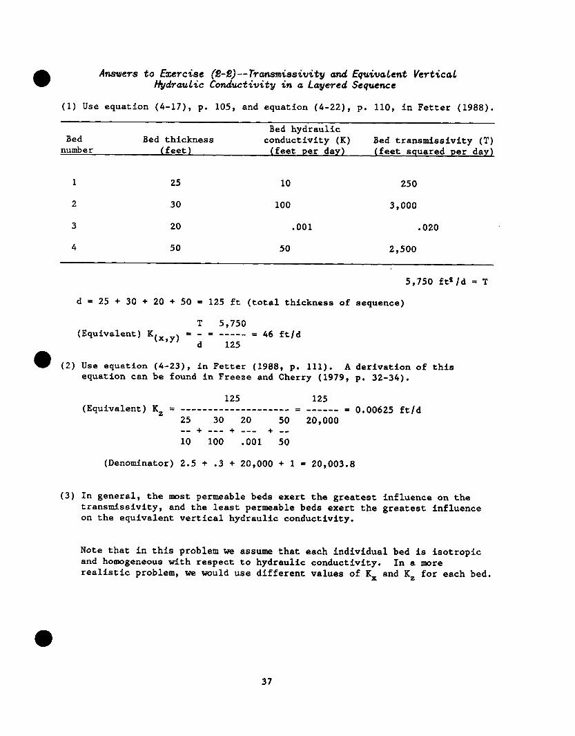
Answers to EZercisc (I%$?) --Transmissivity and Equivalent Vertical Hydraulic Conductivity in a Layered Sequence
(1) Use equation (4-17), p. 105, and equation (4-22), p. 110, in Fetter (1988).
Bed Bed thickness number (feet)
Bed hydraulic conductivity (K) Bed transmfssivity (T)
(feet per day) (feet squared per day)
1 25 10 250
2 30 100 3,000
3 20 .OOl .020
4 50 50 2,500
5,750 fta/d = T
d = 25 + 30 + 20 + 50 = 125 ft (total thickness of sequence)
T 5,750 (Equivalent) K(x,y) = ; = -;;;- = 46 ft/d
(2) Use equation (4-23), in Fetter (1988, p. 111). A derivation of this equation can be found in Freeze and Cherry (1979, p. 32-34).
125 125 (Equivalent) K, = --------------e----- = -w---- = 0.00625 ft/d
25 30 20 50 20,000 -- + --- + --- + -- 10 100 .OOl 50
(Denominator) 2.5 + .3 + 20,000 + 1 t 20,003.8
(3) In general, the most permeable beds exert the greatest influence on the transmissivity, and the least permeable beds exert the greatest influence on the equivalent vertical hydraulic conductivity.
Note that in this problem we assume that each individual bed is isotropic and homogeneous with respect to hydraulic conductivity. In a more realistic problem, we would use different values of Kx and K, for each bed.
37

Aquifers, Confining Layers, Unconfined and Confined Flow
Assignment
*Study Fetter (1988), p. 101-105; Freezeaand Cherry (1979), p. 47-49; or Todd (1980), p. 25-26, 37-45.
The physical mechanisms by which ground-water storage in saturated aquifers or parts of aquifers is increased or decreased (described in the next section) are determined by the hydraulic conditions under which the ground water occurs. In nature, ground water in the saturated zone is found in unconfined aquifers and confined aquifers. The approximate upper bounding surface of the saturated zone is the water table, which is overlain by the unsaturated zone and is subject to atmospheric pressure, whereas confined aquifers are overlain and underlain by confining units. A confining unit has a low hydraulic conductivity compared to that of the adjacent aquifer. Ratios of hydraulic conductivity generally are at least 1,000 (aquifer) to 1 (confining unit), and commonly are much larger. In addition, the head at the top of the confined aquifer always is higher than the altitude of the bottom of the overlying confining unit. This means that the entire thickness of the confined aquifer is fully saturated.
Reference
Lohman (1972b), p. 2, 5, 7 (refer to aquifer; artesian; confining bed; ground water, confined; ground water, unconfined).
38

Ground-Water Storage
Assignments
*Study Fetter (1988), p. 73-76, 105-107; Freeze and Cherry (1979), p. 51-62; or Todd (1980), p. 36-37, 45-46.
*Study Note (2-2)--Ground-water storage.
*Work Exercise (2-3)--Specific yield.
Hydraulic parameters for earth materials can be divided into (1) transmitting parameters and (2) storage parameters. We already have encountered the principal transmitting parameters --hydraulic conductivity (K) or intrinsic permeability (k), and transmissivity (T). In this section the principal storage parameters and specific yield (Sy)--are
--storage coefficient (S), specific storage (Ss), introduced.
The physical mechanisms involved in unconfined storage are different from those involved in confined storage. A change in storage in an unconfined aquifer involves a physical dewatering of the earth materials; that is, earth materials that previously were saturated become unsaturated. When a change in storage takes place in a confined aquifer, the earth materials in the confined aquifer remain saturated.
Reference
Lohman (1972b), p. 12, 13 (refer to specific retention; specific yield; storage, specific; storage coefficient).
Comments
The treatment of aquifer and water compressibility and effective stress in Freeze and Cherry (1979, p. 51-58) is too detailed for presentation in this course, but it provides the necessary background for any level of discussion on storage in confined aquifers that the instructor chooses to undertake. Key concepts are the fundamentally different physical mechanisms controlling changes in storage in unconfined and confined aquifers and the related large differences in storage coefficients between these two aquifer types.
39

Answers to Exercise (2-S) --Specif ic Yie Id
A rectangular prism whose base is a square with sides equal to 1.5 ft and height equal to 6 ft is filled with fine sand whose pores are saturated with water. The porosity (n) of the sand equals 34 percent. The prism is drained by opening a drainage hole in the bottom and 2.43 fta of water is collected. Calculate the following quantities:
total volume of prism 1.5 ft x 1.5 ft x 6 ft = 13.5 fts
volume of sand grains in prism .66 x 13.5 = 8.91 fta
total volume of water in prism before drainage .34 x 13.5 = 4.59 ftr
volume of water drained by gravity 2.43 ftg
volume of water retained in prism (not drained by gravity)
4.59 - 2.43 = 2.16 fta
specific yield 2.43113.5 = .18
specific retention 2.16/13.5 = .16
0.34 By definition, specific yield + specific retention = porosity (n).
40

(1) Assuming the value of specific yield determined above, what volume of water, in cubic feet, is lost from ground-water storage per square mile for an average 1-ft decline in the water table?
VW = SAAh (equation (4-21), Fetter (1988, p. 107))
VW = .18 x 5,280 ft x 5,280 ft x 1 ft = 5,018,112 fta
Express this volume as a rate for 1 day in cubic feet per second.
5,018,112 ft8 -..------------ = 58.08 ft?/s
86,400 s
Express this volume as depth of water in inches over the mi2.
.18 x 12 in. = 2.16 in.
(2) Assuming the value of specific yield determined above, a volume of water added as recharge at the water table that is equal to (a) 1 in. and (b) 4.8 in. per unit area would represent what average change in ground-water levels, expressed in feet?
VW = SAAh
SA ft
(a) 1 ft2 x 1 in. x ------ 12 in.
Ah = ----------_--__-___--- = .463 ft . 18 x 1 ft2
ft (b) 1 ft' x 4.8 in. x ----em
12 In. Ah = ------------------------- St 2.22 ft
. 18 x 1 fta
41

Ground-Water Flow Equation
Assignments
*Study Fetter (1988), p. 131-136; Freeze and Cherry (1979), p. 63-66, 174-178, 531-533; or Todd (1980), p. 99-101.
*Study Note (2-3)--Ground-water flow equation.
*Define the following terms by referring to any available mathematics text that covers differential equations--independent variable, dependent variable, order, degree, linear, nonlinear.
A differential equation that describes or "governs" ground-water flow under a particular set of physical circumstances can be regarded as a kind of mathematical model. In ground-water flow equations, head generally is the dependent variable. If the flow equation is solved, either analytically or numerically, values of head can be calculated as a function of position in space in the ground-water reservoir (coordinates x, y, and z) and time (t). The differential equatfion provides a general rule that describes how head must vary in the neighborhood of any and all points within the flow domain (ground- water flow system). Numerical algorithms that are amenable to solution by digital computers (for example, the finite-difference approximation of a differential equation) can be developed directly from the differential equation.
The ground-water flow equation developed in Note (2-3) is widely applicable. Note that the steady-state form of this equation represents the mathematical combination of (1) the equation of continuity and (2) Darcy's law.
Comments
Many students with weak backgrounds in mathematics "tune out" whenever they see a derivative, not to mention a differential equation. The role of the instructor in discussing Note (2-3) on the ground-water flow equation is to help the participants interpret the mathematical notation and continue beyond it to the underlying physical concepts in the derivation, which were introduced previously in this course. The mathematical notation can be regarded as a powerful "shorthand" language for expressing physical relations.
As a follow-up to the idea that a differential equation used to describe a ground-water system or problem contains important physical information on an investigator's assumptions about that system or problem, participants will benefit greatly from discussion of and practice in what can be termed "differential-equation recognition." Specifically, participants will benefit from learning to identify in the differential equation features such as (1) *dependent and independent variables; (2) dimensionality of flow system (one-, two-, or three-dimensional); (3) steady versus unsteady flow; (4) identification of parameters (hydraulic conductivity (K), transmissivity (T), storage coefficient (S), specific storage (S,), aquifer thickness (b or m), and area1 recharge (W)); and (5) the presence or absence and the position of the conductive parameter (K or T) in the equation, which indicates the
42

assumptions of the investigator concerning the properties of the earth material in the system under study--for example, the earth material is isotropic and homogeneous, anisotropic and homogeneous, or anisotropic and heterogeneous. In reports on ground-water studies, the ground-water-flow equation that is used in the quantitative analysis usually is written in only four or five different ways , not including possible minor variations. Several of these ways are simplifications of the flow equation derived in Note (2-3). Examples of often-used equations and their corresponding assumptions follow.
(1) 6'h 6ah --- + --- = 0 8x2 6i9
(h is dependent variable, x and z are independent variables; two dimensions; steady flow; flow medium is isotropic and homogeneous; flow domain is a vertical section)
Ph Ph (2) K, --- + K, --- = 0
8x2 69
(same as (1) except medium is anisotropic and homogeneous)
t3) %; (Kx ;;) + %; (Kz !) = o
(same as (1) except medium is anisotropic and heterogeneous)
(dependent variable h, independent variables x, y, t; two dimensions; unsteady flow; T varies in x and y directions; flow is horizontal, or nearly so)
43

(5) d*h -W --- = -- dxg T
(dependent variable h, independent variable x; one dimension; steady flow; T is constant; because only one independent variable (x) appears in the
d2h equation, the ordinary differential notation --- is used instead of the
@h dx2 partial differential notation --- )
6X2
The terms of a differential equation that describe a physical process must exhibit
equations in
d2h [L-l] (;;; =
consistent physical dimensions in the same way as any other d2h
physics. For example, the term --- has the dimensions of dx'
d dh -- --
( 1) , and ,p (TX %q, has the dimensions of [LT'I]. dx dx

SECTION (3)--DESCRIPTION AND ANALYSIS OF GROUND-WATER SYSTEMS
The first three subsections below--system concept, information required to describe a ground-water system, and preliminary conceptualization of a ground-water system--introduce the system concept as it is applied to ground- water systems. The system concept is exceedingly useful in ground-water hydrology. It provides an organized and technically sound framework for thinking about and executing any type of ground-water investigation and is the basis for numerical simulation of ground-water systems, the most powerful investigative tool that is available. Although the system concept usually is not developed in a beginning course in ground-water hydrology to the extent that it is here, its fundamental importance , particularly as a framework for :hinking about a ground-water problem, warrants this emphasis.
An example of the need for "system thinking" in practical problems is the "site" investigations of ground-water contamination from point sources, a major activity of hydrogeologists at this time. Many of these studies suffer irreparably from the investigators' failure to apply "system thinking" by not placing and studying the local "site" in the context of the larger ground-water system of which the "site" is only a small part.
System Concept
0 Assignment
*Study Note (3-1)--System concept as applied to ground-water systems.
In Note (3-l), attend particularly to the list of features that characterize a ground-water system. Although these features may seem to be abstract at this time, the reasons for this formulation will become evident as we proceed.
Reference
Domenico (1972), p. 1-21.
Comments
From the standpoint of this course, the content of Note (3-l), although brief, is designed to be self-contained. A much broader perspective on the system concept is provided by Domenico (1972, p. 1-21).
45

Information Required to Describe a Ground-Water System
Assignments
*Study Fetter (1988), p. 533-534; or Freeze and Cherry (1979), p. 67-69, 534-535.
*Study Note (3-2) --Information necessary to describe a ground-water system.
In these and other study assignments, concentrate particularly on all the available information about the boundary conditions used in ground-water hydrology (name, properties, and physical occurrence in real ground-water systems). This is the most important new information in this section and also the most difficult to apply to specific problems.
Reference
Franke, Reilly, and Bennett (1987), p. l-10, 14-15.
Comments
The discussion in Note (3-2) on the information necessary to describe a ground-water system can begin profitably with a patient review of table (3-l). With the help of the class, make a list of the common natural and human stresses on ground-water systems.
Because we routinely measure heads in the field, we are most aware of and, thus, regard changes in head as the principal response to stress in ground-water systems. Our best opportunity to measure changes in ground-water flow in response to stress is to monitor changes in base flow of streams. Unfortunately, interpretable base flow data commonly are not available for this purpose unless a special program of data collection is established--for example, a systematic series of periodic base-flow measurements.
Among the pertinent features of a ground-water system listed in table (3-l) of Note (3-2), beginning hydrologists have the greatest conceptual difficulty with boundary conditions. Adequate information on boundary conditions for this course is provided by Franke and others (1987). Distinguishing between physical boundary conditions--that is, a description of actual hydraulic conditions at the boundaries of the ground-water system in the field--and mathematical boundary conditions, which usually are a highly idealized and simplified representation of these conditions, is essential for an overall understanding of boundary conditions by participants. In fact, at this juncture in the course, the discussion of physical boundary conditions is as important as the discussion of mathematical boundary conditions. For example, ground-water recharge to the water table is intermittent and highly variable in space and time, both during the annual hydrologic cycle of a given year and from year to year. However, we often treat area1 recharge as a constant-flux boundary in analytical solutions and numerical simulations--that is, estimates of actual recharge are averaged for a period of years, and this average flux is applied to a model of the natural ground-water system.
We recommend that instructors review all aspects of boundary conditions at every opportunity during the rest of this course , particularly in relation to concrete examples.
46

Preliminary Conceptualization of a Ground-Water System
Assignments
*Study Note (S-3)--Preliminary conceptualization of a ground-water system.
*Work Exercise (3-1)--Refining the conceptualization of a ground-water flow system from head maps and hydrogeologic sections.
*Refer to figure l-7 of Note (l-l) on head, in which three pairs of observation wells are depicted, each pair illustrating a different relation between shallow heads and deeper heads. On the basis of your study of the ground-water system in Exercise (3-l), where would you expect to find each pair of observation wells in a "typical" ground-water system, irrespective of the scale of that system?
After finishing the assignments, note that (1) our conceptualization of a ground-water system is based on what we know about that system at any particular time and must be revised continually as new information becomes available; and (2) a system conceptualization that bears little resemblance to the real system under study may lead to quantitative analyses of that system that are grossly in error because, in essence, the "wrong" system is being analyzed.
Reference
Freeze and Cherry (1979), p. 193-203.
Comments
Table 3-l in Note (3-2) on information necessary for definition of a ground-water system and table 3-2 in Note (3-3) with steps for developing a conceptual model of a ground-water system provide a general, although somewhat abstract, framework for thinking about a ground-water system or problem. Applying this general, conceptual framework to a specific ground-water system requires practice and a general knowledge of ground-water hydrology. We must expect that most course participants will be lacking in both prerequisites. The first ground-water system to be studied in considerable detail in this course is described and analyzed in Exercise (3-l). We reconanend that the two tables referred to above be used as guides and referred to explicitly in all discussions by the instructor on this ground-water system so that participants will learn what the information in the tables means through application to a concrete example.
Exercise (3-l) consists of three parts: (1) analysis of the unstressed system (questions 1 to 5), (2) analysis of the system stressed by a pumped well (question 6), and (3) analysis of a system that is similar to that in parts (1) and (2) except that the confining layer is discontinuous rather than continuous. We recommend that at least parts (1) and (2) be completed during the course.
47

Answers to Exercise ($-1)--Refining the Conceptualization of a G+round-Water Flow System from Head Maps and Hydrogeologic Sections
The purpose of this exercise is to demonstrate (1) how the three- dimensional distribution of hydraulic head in a ground-water system can be depicted accurately on a series of maps and sections derived from (a) pertinent hydrologic data, (b) knowledge of the physics of ground-water flow, and (c) a preliminary conceptualization of the structure and operation of a ground-water system; and (2) how this depiction of the head distribution either is a con- firmation of our initial conceptualization of the system or includes a modifi- cation of our initial conceptualization. The modification process is based on the results of the mapping analysis and the data utilized, and indicates an evolution in our level of understanding of the ground-water system. Inherent in item 2 is the implication that the complete integration of available hydrologic data, knowledge of physics, and hydrologic experience in the mapping analysis can improve our understanding of a ground-water flow system.
This mapping exercise is a qualitative analysis of the available data and undoubtedly is subject to some subjectivity and the professional judgment of the hydrologist making the analysis. Nonetheless, as we point out throughout the exercise, the knowledge and experience of the hydrologist must be incorporated into the final conceptualization of the ground-water system so that it represents a complete integration of the three factors listed above.
Head maps commonly are used to interpret the behavior of ground-water systems. Head maps are used to evaluate the direction and rate of ground- water flow within an aquifer; Head maps of layered aquifers commonly are used to estimate zones of upward and downward flow between the aquifers. Head maps for different hydrologic conditions can be compared to evaluate the response character of a ground-water system. The accuracy of such interpretations depends on the degree to which an understanding of the operation of the ground-water system is incorporated in the mapping exercise.
Perhaps the most demanding application of head maps and sections is their use in the calibration of ground-water-flow-simulation models. In this case, a model's ability to represent the structure and operation of a ground-water flow system is assessed largely on the basis of its ability to reproduce the three-dimensional distribution of hydraulic head in the system as depicted by maps and sections of observed head. The model integrates the physical laws that govern ground-water flow with the charatiteristics of the ground-water system--its boundary conditions, its hydrogeologic framawrk (geouwtry), the distribution of water-transmitting properties, and the presence of any internal ground-water sources or sinks. Head maps that are constructed without consideration of these factors are not an accurate representation of the flow system and are not a suitable gage with which to evaluate the validity of a ground-water model.
48

The mapping exercise consists of three parts. The first part "Mapping hydraulic head in a layered ground-water system," presents the mapping problem as a sequence of steps. It begins with mappIng the water table, continues with mapping the potentiometric surface in the confined aquifer, and ends with mapping the hydraulic head in selected sections. The instructions repeatedly suggest the advisability of returning to maps already drawn and modifying these maps on the basis of the information gained from subsequent maps or sections and the associated data. This stepped approach is used in this part of the exercise to reinforce two important considerations:
(1) The head map and section sets represent a complete picture of hydraulic head in the ground-water system and, therefore, should be constructed concurrently; and
(2) even sparse head data for an aquifer can be used to define the head surface in the aquifer when considered together with head data for overlying or underlying aquifers.
The final product of the set of head maps and sections is a depiction of the three-dimensional distribution of hydraulic head in the ground-water system. To reinforce this fact, the instructor should point out that contour
.lines, which conventionally are considered to be a linear expression on a two- dimensional surface, are in reality contour surfaces through three-dimensional space. A contour line is the expression of that three-dimensional three- dimensional surface in the plane of the map or section. An understanding of the three-dimensional nature of ground-water systems, in terms of their framework, boundaries, water-transmitting properties, head distributions, flow
0 patterns, and related heterogeneities, is arguably the most critical factor in achieving an understanding of the structure and operation of a ground-water system.
The second part of the exercise, "Mapping hydraulic head in a layered ground-water system with a pumped well," is designed to demonstrate the added understanding of a ground-water system that is gained from analyzing and comparing hydraulic heads under stressed and unstressed conditions. The third part of the exercise, "Mapping hydraulic head in a layered ground-water system with a discontinuous confining unit," presents a case in which the observed- hydraulic-head data are inconsistent with our original conceptualization of the ground-water system and which involves reformulation or refinement of our flow-system concept as part of the mapping exercise.
The following sections provide detailed solutions to all three parts of the head-mapping exercise. This exercise provides an opportunity that is not available in field investigations of ground-water systems--that is, the opportunity to compare the student's interpretation of sparse hydrologic data to an exact solution of the head distribution within the system. The hypothetical ground-water systems presented in this exercise were represented exactly in a numerical ground-water-flow-simulation model. The locations of observation wells were established at model nodes, head data for each synoptic measurement were taken from specific steady-state-model simulation results, and the answer map and sections were constructed from complete simulation results. Thus, the system concept presented and suggested for use in constructing the head maps and sections is virtually an exact replica of the system under study, whereas results of field investigations never replicate the real system exactly.
49

In field investigations of ground-water system8 , no exact solutions exist. Conceptual models are never exact, but are crude and grossly simplified approx imations of the real system. These simplifications are found in both system
d
detail and hydrologic condition. Features of system detail that can never be defined fully in our conceptual model include details of boundary representa- tion, hydrogeologic framework, and variations in water-transmitting properties that are present at a finer scale than can be measured and mapped with avail- able data. Simplifications of hydrologic condition involve the assumption that the observed data approximate a steady-flow condition within the aquifer system. Synoptic head measurements undoubtedly are affected to some degree by the dynamic nature of ground-water systems, and express the effects of seasonal fluctuations, longer-term climatic trends, or variations in pumping rates. Consideration of such complexities in mapping head in actual field investiga- tions is virtually impossible but adequate design of monitoring programs can minimize their effect. An adequate monitoring network can provide indirect information about the scale of heterogeneities that is relevant to the objectives of the analysis. Synoptic measurements can be scheduled to provide a picture (measure) of the hydrologic system that is consistent with the hydrologic condition being analyzed.
The remainder of this discussion consists of detailed answers to specific questions in Exercise (3-l).
Question 1 .--Boundary condition8 must be represented over the entire external boundary surface of the ground-water flow system. The maps and sections in figure 3-2 provide a three-dimensional picture of the system and its boundary surface. The boundary conditions on the boundary surface are as follows: The contact between the aquifer system and bedrock is assumed to be a no-flow, or streamline, boundary; the water table is assumed to be a free-surface and a constant-flux boundary, where recharge from precipitation enters at a constant rate and the water-table surface can move in response to change8 in hydrologic conditions; the surface ofdcontact between the aquifer system and the surface water in the lake (lake bottom) is assumed to be at a constant head that is equal to the stage of the lake; the contact between the aquifer system and the streambed is assumed to be a head-dependent-flux boundary, where the ground-water discharge to the stream is controlled by (1) the difference in head between the stream stage and the head in the surrounding aquifer, and (2) the hydraulic properties of the streambed and adjacent aquifer material.
Mapping hydraulic head in a layered ground-water system
6jM3tiOBS 8 t0 b.--Questions 2, 3, and 4 relate to mapping hydraulic head in the unconfined aquifer, in the confined aquifer, and on two sections, respectively. Because all the maps and sections are constructed jointly, the di8cu88ion8 of these question8 are presented together. Figures 3-4, 3-6, 3-7, and 3-8 present the distribution of hydraulic head for the water table, confined aquifer, and sections A and B, respectively.
50

The water-table contour lines (fig. 3-4) depict gradients that increase toward the shoreline and represent a water-table configuration that shows the effects of two factors: With proximity to the shoreline, (1) the amount of water flowing through the system continually increases as a result of accretion from recharge, and (2) the transmissivity of the aquifer decreases as the water table approaches the lake level. In addition, the shape of contours near boundaries is consistent with our concept of boundary operation. Contours approach impermeable boundaries at right angles, tend to parallel constant-head boundaries, and "V" upstream at the gaining stream. The S- and lo-ft contours intersect the stream channel very near the locations where the streambed altitudes are 5 and 10 ft, respectively. (In this contouring exercise we are assuming that the depth of the stream is negligibly small. If the assumed stream depth were to increase, the points where the S- and lo-ft water-table contours intersect the stream would move further downstream from the 5- and lo-ft streambed altitudes.) However, the 15- and 20-ft contours cross the stream upstream from the locations of the 15- and 20-ft streambed altitudes, respectively, because the stream start-of-flow is located south of the 15- and 20-ft streambed altitudes --that is, the streambed is dry at these altitudes, and the water table must lie below the streambed in this stream reach.
The potentiometric surface in the confined aquifer (fig. 3-6) also shows contours that approach boundaries in a manner that Is consistent with their basic hydrologic interpretation. A subtle depression in the potentiometric surface is centered on the stream, reflecting the increased depression in the water table near the stream. This depression in the potentiometric surface is
0
consistent with the interpretation that flow converges toward this area and discharges upward to the overlying aquifer in the area of depressed heads surrounding the stream channel. Note in figure 3-4 that the transition from downward to upward flow between these aquifers shifts upstream beneath the stream.
51

Answer to Ekercisc ($-I), Question I!
l 32.47.
a 30.66
Lake 0 2 MILES
++-- 0 2 KiLOMiTERS
A EXPLANATION
l 9.9 WATER-TABLE OBSERVATION WELL -- Number is altitude of water level, in feet above sea level
k
5 STREAMBED LEVEL -- Number is elevation of streambed, in feet above sea level
k- POINT OF START-OF-FLOW OF STREAM
A-A’ TRACE OF SECTION
-5- WATER-TABLE CONTOUR
- - LINE OF DEMARCATION BET WEEN REGION IN WHICH GROUND-WATER FLOW EXHIBITS A DOWNWARD COMPONENT AND REGION IN WHICH IT EXHIBITS AN UPWARD COMPONENT

Answer to Ezrcise (3-l), Question 3
l 28.32
0 29.48 .27.28
Lake
/-- -------- \ l 6.92 -/-- > 2 KILOMETERS --- -H-d
A
EXPLANATION
0 6.92 OBSERVATlON WELL SCREENED IN THE CONFINED AQUIFER -- Number is altitude of water level, in feet above sea level
A-A’ TRACE OF SECTION
-15- HEAD CONTOUR
---- -- TRACE OF SHORELINE AND STREAM AT LAND SURFACE
a Figure 3-6.--Head contours in the confined aquifer drawn from results of a synoptic measuremen? of water levels in observation wells:
53

Head contours in section A-A' (fig. 3-7) are effectively vertical in both the unconfined and confined aquifers and refract upon entering the confining unit. The slope of the contours within the confining unit reflects the magnitude of the vertical gradients across the unit. The maximum downward gradient is found at the northern end of section A-A'. Moving south along the section, vertical gradients gradually decrease to zero at the line of demarcation between regions of upward and downward flow, reverse to upward, and gradually increase to a maximum upward gradient beneath the lake discharge boundary. The spacing of contours in the confined aquifer in both the section and the map (figs. 3-6 and 3-7) shows a maximum horizontal gradient (i.e. the closest spac‘ing of contours) near the line of demarcation from upward to downward flow, where the maximum amount of flow in the confined aquifer would be expected. 5
The head distribution in section B-B' is shown in figure 3-8. This section trends almost parallel to the head contours and, thus, can show significant differences in head distribution and associated flow patterns because of subtle differences in contouring. The head contours show a downward gradient at the western edge of the section that gradually decreases and then reverses to an upward gradient beneath the stream, and possibly reverses again at the extreme eastern edge of the section. Very large upward vertical gradients are present beneath the stream channel in the unconfined aquifer. These vertical gradients are reflected by the lo-ft contour, which sweeps under the stream, whose altitude is less than 7 ft above sea level at that location. Note that the shape of the lo-ft contour resembles the shape of the streambed, which is a constant-head boundary.
54

S A
FEET 40-
SEA LEVEL
40-
1
60-
160-
I- 6.92
1aoI
AQUIFER
lIIzl ,:_::;:_ _:. :. :_ ,: : 1: CONFINING UNIT
t ?
25.06
II c
EXPLANATION
-25- HEAD CONTOUR
+ + APPROXIMATE DIRECTION OF GROUND-WATER FLOW -- LINE OF DEMARCATION BCTWEEN REGION IN WHICH
GROUND-WATER FLOW EXHIBITS A DOWNWARO
Y WELL LOCATION -- Horizontal lines COMPONENT AND REGION IN WHICH IT EXHIBITS
17.43 represent separate screened zones. AN UPWARD COMPONENT Number is altitude of water level, in feet above sea level
Figure 9-7. --North-south-trending hydrogto logic section showing head contours
l dram from results of a synoptic measurement of water levels in observation wells. (L oca t ion of section A-A' is shown in fig. S-8.)
55

W B
FEET
---
SEA _ LEVEL
20-
120-
140-
160-
Answer to Exercise (9-l), Question 4
19.58 I
17.43 1 14.52
0
i 0
EXPLANATION
AQUIFER -2+ HEAD CONTOUR
i -
$$&g;r CONFINING UNIT + APPROXIMATE DIRECTION OF GROUNLhWATER w
. . . ..i..i -- LINE OF DEMARCATION BETWEEN REGION IN WHIo(
WELL LOCATION -- Horizontal lines represent separate screened zones Number is altitude of water level, in feet above sea level
GROUND-WATER FLOW EXHIBITS A DOWNWARD COMPONENT AND REGION IN WHICH IT EXHIBITS AN UPWARD COMPONENT
Figure 3-8. --East-west-trending hydrogrologic m&ion ahowing head contow dram from results of a qfwptic wamwabent of v&w tmd8 irr observation wells. (L oca ion ef aactisr, 8-F 4a whom in fi;B. t
56

An additional question can be posed by the instructor after this part of the mapping exercise has been completed: How does the area through which water enters the confined aquifer (the area of downward flow across the overlying confining unit) compare with the recharge area of the confined aquifer? (The recharge area of the confined aquifer is the area on the water table that contributes recharge to the ground-water system that ultimately enters and flows through the underlying confined aquifer.)
This question is intended to prompt discussion on the way the flow system operates and can be considered in two ways: (1) in a budget sense, and (2) in a flow-path sense. In a budget sense, because the recharge rate is uniform over the water table, the recharge area of the confined aquifer is a percentage of the recharge area of the entire system (the area of the water-table boundary) that is equal to the percentage of the flow in the entire ground-water system that enters the confined aquifer. The distribution of aquifer properties and the hydrogeologic framework of this system indicate that most of the water that recharges this ground-water flow system remains in the unconfined aquifer and discharges directly to the lake and tributary-stream boundaries. In this case, the recharge area of the confined aquifer is considerably smaller than the area of downward flow across the confining unit, as shown in figure 3-4.
To address this question in a flow-path sense, consider the selected flow paths shown on section A-A' (fig. 3-9). The line of demarcation between downward and upward flow across the confining unit marks the location of a flowline that separates water that enters the confined aquifer (represented by all flowlines that enter the system to the north of and flow below this flowline) from water that flows only in the unconfined aquifer (represented by all flowlines that enter the system to the south of and flow above this flowline). The flow pattern in figure 3-9 indicates that the recharge area of the confined aquifer is in the northernmost part of the ground-water system.
57

s A
FEET 40-
SEA _. LEVEL
140-
160 -
AREA OF DOWNWARD FLOW TO CONFINED AQUIFER
1 RECHARGE AREA OF N CONFINED AQUIFER
160 ’ c
EXPLANATION
II AQUIFER
CONFINING UNIT
- FLOWLINE
- - LINE OF DEMARCATION BETWEEN REGION IN WHICH GROUND-WATER FLOW EXHIBITS A DOWNWARD COMPONENT AND REGION IN WHICH IT EXHIBITS AN UPWARD COMPONENT
Figure 3-Q. --Conceptual diagram of flow patterns along north-south-trending hydrogeologic sections comparing the recharge area of the confined aquifer at the water table with the area of downward floti to the confined aquifer at the top of the confining unit. (Location of section A-A’ is shown in fig. S-2.)
a
58

Mapping hydraulic head in a layered ground-water system with a pwnped well
Unnumbered questions .--The only difference between the unstressed system previously mapped and this system is that a well has been introduced that is withdrawing approximately 8 percent of the natural flow in the ground-water system. [The area of the ground-water system through which recharge enters (i.e. the area of the water table) is approximately 56,000 ft by 40,000 ft, or 2.24 x lo9 fta. The rate of area1 recharge is approximately 0.475 ft/yr. Therefore, total recharge to the system equals the recharge rate times the area, which is 1.064 x lo9 fta/yr or 21.8 Mgalld. The well pumps at a rate of 1.66 Mgal/d, or 7.6 percent of the total natural recharge to the system.]
For purposes of this exercise, we assumed that the system is in equilibrium with the pumping stress. Therefore, the drawdown from the pumped well has reduced gradients to the stream and the lake, effectively diverting water to the well that otherwise would have discharged to these boundaries. The effect of a pumped well on heads and flows in a ground-water system is discussed further in Exercise (3-3), "Source of water to a pumped well."
Question 6 .--Figures 3-10, 3-11, and 3-12 show the mapped steady-state head distribution in this system with a well that is pumped at a steady rate. A simple but critical concept in this analysis is that, neglecting other possible hydrologic changes that could be detected in the monitoring program, the difference between this head distribution and that in the previous part of this exercise has been caused by the pumped well. Stated in another way, the head distribution in the system with the pumped well is the sum of the head distribution without the well (figs. 3-4, 3-6, 3-7, 3-8) plus the drawdown caused by the pumped well. Therefore, the head distribution in the unstressed system should be used as a guide in contouring the head distribution in the stressed system. If this procedure is not followed, subtle differences in subjective manual contouring of the data could result in differences between the head distribution for stressed and unstressed conditions that could be attributed erroneously to the effects of the pumped well.
59

In figure 3-10, a closed 25-ft contour line has been drawn arbitrarily around the pumped well on the water-table map to indicate a closed depression around the well. Although the shape of this depression is not accurately defined, the data point immediately south of the pumped well with an observed head value of 25.07 ft indicates that (1) the water-table altitude exceeds 25 ft above sea level south of the pumped well (so that the main 25-ft contour does not trend north and enclose the pumped well), and (2) the head in the cone of depression near the pumped well undoubtedly is less than 25 ft above sea level. The head distribution in section A-A' (fig. 3-12) shows the configuration of the closed 25-ft contour in vertical section. The shape of this three-dimensional surface of equal hydraulic head is approximately cylindrical and is centered at the pumped well. It probably extends farther from the well at a depth equivalent to the screened interval of the pumped well, but the data are insufficient to map explicitly at this level of detail.
The line of demarcation between downward and upward flow across the confining unit indicates a slight shift from unstressed to stressed conditions (figs. 3-4 and 3-10, respectively). The well diverts some water from flowing down to the confined aquifer. The drawdown caused by pumping the ~11 is greatest in the northwestern part of the system. As a result, both downward flow to the confined aquifer and upward flow from the confined aquifer occur at a significantly reduced rate compared to flow under unstressed conditions. (The head change across the confining unit at the northwesternmost observation well decreases from 5.6 ft under unstressed conditions to 4.5 ft under stressed conditions.)
An additional exercise that provides further insight into the effect of the pumped well on the system is to calculate the drawdown at each observation well in the unconfined aquifer from heads in the stressed and unstressed systems (figs. 3-10 and 3-4) and to contour these data.
60

A’
Answer to Exercise (8-l), question 6
l 31.26
. 28.94
\ ’ -/
l 25.07
I l a.18
Lake 0 1 2 MILES
-7 0 2 KILOMETERS
! EXPLANATION
A-A’ TRACE OF SECTION 0 a.18 WATER-TABLE OBSERVATION WELL -- Number is altitude
-5- WATER-TABLE CONTOUR of water level, in feet above sea level
- - LINE OF DEMARCATION BETWEEN REGION k
5 STREAMBED LEVEL -- Number is elevation of streambed IN WHICH GROUND-WATER FLOW EXHIBITS in feet above sea level A DOWNMEARD COMPONENT AND REGION IN WHICH IT EXHIBITS AN UPWARD COMPONENT - POINT OF START-OF-FLOW OF STREAM
@ PUMPED WELL
Figure 3-10. --Measured heads in the unconfined aquifer caused by response to steady pwnping from a well screened in the lower part of the unconfined aquifer .
61

Answer to Exercise (3-l), Question 6
l 26.2
0 25.99
B-
I A EXPLANATION
06.26 OBSERVATION WELL SCREENED IN CONFINED AQUIFER -- Number is altitude of water level, in feet above sea level
A-A’ TRACE OF SECTION
-lO- HEAD CONTOUR
- - - - -- TRACE OF SHORELINE AND STREAM AT LAND SURFACE
l 23.09
0 22.03 I
I
-20 I I I \
\ \
\
015.55 - -I5 \ I I
I
/--do- I
L -------w------------------------d ' \-----,-- ------ --
f
Lake
/-- -;6;c---_) \ 2 KILOMETERS
-- -/-- ,/--
-8
0
Figure 3-11. --Measured heads in the confined aquifer cuwcd by rcspon~ to steady pumping from a well screened in the lower part of the unconfined aquif cr. a
62

Answer to Ekercisc (S-l), Question 6
0 FEET
40
160
180
I AQUIFER
CONFINING UNIT
EXPLANATION
0
i 0
I- 25.88
2 MILES
KILOMETERS
-25- HEAD CONTOUR
- - APPROXIMATE DIRECTION OF GROUND-WATER FLOW
-- LINE OF DEMARCATION BETWEEN REGION IN WHICH
e
WELL LOCATION -- Horizontal lines represent separate screened zones.
**.03 Number is altitude of water level, in feet above sea level
GROUND-WATER FLOW EXHIBITS A DOWNWARD COMPONENT AND REGION IN WHICH IT EXHIBITS AN UPWARD COMPONENT
Figure 3-1s .--North-south-trending hydrogeologic section showing head contours
a
drawn from measured head.s caused by response to (Location of sect$on A-A' is shown in fig. S-2.)
steady pumping.
63

Mapping hydraulic head in a Layered ground-water system with a discontinuous confining unit 0
question 7.-- Field observations of hydraulic head frequently are inconsistent with our basic conceptualization of the ground-water system. In this exercise, the near-absence of vertical gradients between the unconfined and confined aquifers in an area where vertical gradients are expected to be greatest has caused us to reformulate our concept of the system. Perhaps these unexpected head data prompted collection of additional surface- geophysical information or borehole geophysical logs that indicated an absence of the confining unit in the extreme northwestern part of the area.
Overlaying the water-table and potentiometric-surface maps (figs. 3-13 and 3-15) reveals that the 30-ft contour lines on both maps are parallel and coincident in the area where the confining unit is absent (referred to as a "hole" in the confining unit). The vertical head drop in the absence of the confining unit is on the order of a hundredth of a foot. Although vertical gradients are small, downward flow through the hole may be significant because the vertical hydraulic conductivity of the aquifer material is much greater than that of the confining unit. In fact, the head data indicate that the hole is a pathway for downward flow to the confined aquifer. The 30-ft contour on the water table bends slightly southward on either side of the hole. These contours depict a water table with a slight depression over the hole in the confining unit , and indicate that water flows toward the hole and downward through the hole to the underlying aquifer.
The 30-ft contour line on the head map of the confined aquifer (fig. 3-15) bends to the north on either side of the hole. This contour shape indicates that water enters the confined aquifer through the hole and forms a small mound in the potentiometric surface from which water disperses within the confined aquifer. The distance between the 30-ft contour line on the water-table map and the 30-ft contour line on the potentiometric-surface map increases rapidly eastward of the hole, indicating a consistent increase in the vertical gradient between the two aquifers with distance from the hole. The head distribution on section A-A ‘ (fig. 3-16) depicts a very small change in head between the two aquifers where the confining unit is absent. (The 30-ft contour is virtually vertical.)
Logic suggests that a greater amount of water flows to the confined aquifer with the hole in the confining unit than in the original system. As a result, heads both beneath the lake discharge boundary and in the area of upward flow from the confined aquifer are greater in the hypothetical system with the hole in the confining unit than in the system without the hole in the confining unit (compare figures 3-6 and 3-15, and figures 3-4 and 3-13). The hole allows a significant increase of flow down to the confined aquifer over a small area; the resulting increase in discharge from the confined aquifer requires increased upward gradients and a larger discharge area.
64

B-
Anstoer to Exercise (3-l), Question 7
A' I
0 33.77 l 32.45
l 28.82
* 8.92 A/
Lake
2 KILOMETERS
I I
A EXPLANATION
l 8.92 WATER-TABLE OBSERVATION WELL -- Number is altitude of water level, in feet above sea level
k 5 STREAMBED LEVEL -- Number is elevation ot
\
streambed, in feet above sea level
c POINT OF START-OF-FLOW OF STREAM
A-A’ TRACE OF SECTION
-2o- WATER-TABLE CONTOUR
- - LINE OF DEMARCATION BETWEEN REGION IN WHICH GROUND-WATER FLOW EXHIBITS A DOWNWARD COMPONENT AND REGION IN WHICH IT EXHIBITS AN UPWARD COMPONENT
a Figure 3-13 .--Measured heads in the unconfined aquifer in a ground-water system with a dimontinuous confining unit.
65
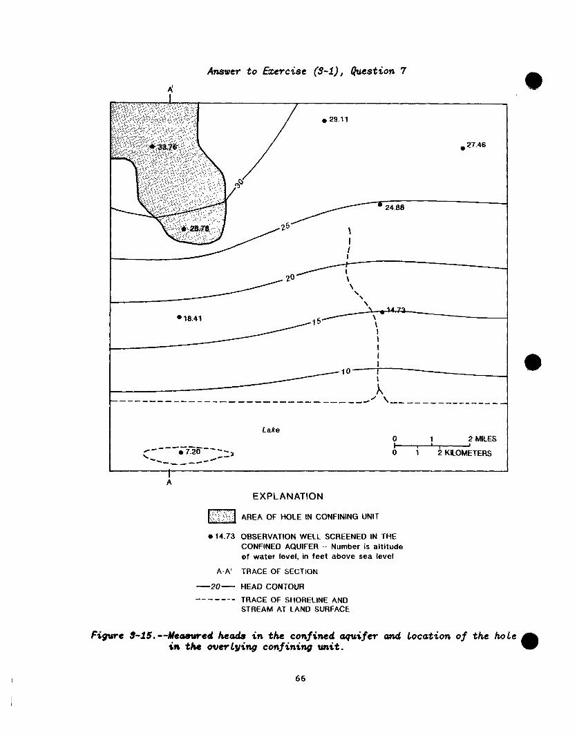
A~~surer to EXWC~S~ (3-l), &&ion 7
l 18.41 15 \ I I I
I 10
L -------------------------------~ ‘\ -we-------------
Lake 0 2 MILES
/----------2 \
l 7.20 0’-;-1’---’ -- -c--- *de-
3 2 KILOMETERS
I A
EXPLANATION
1::. .’ L i ,. Tclc( 1, :~.:.A. +., p ,. ?.’ AREA OF HOLE IN CONFINING UNIT
l 14.73 OBSERVATION WELL SCREENED IN THE CONFINED AQUIFER -- Number is altitude of water level, in feet above sea level
A-A’ TRACE OF SECTION
-2o- HEAD CONTOUR ------- TRACE OF SHORELINE AND
STREAM AT LAND SURFACE
Figure 3-15.--kaswrcd heads in the confined aquifer and location of the hole in the overlying confining unit. a
66

Answer to Ezercisc (S-I), Question 7
S
0 A
FEET
.
!8.78
1 ? MILES
2 KILOMETERS
EXPLANATION
AQUIFER
CONFINING UNIT
-2o- HEAD CONTOUR
* * APPROXIMATE DIRECTION OF GROUND-WATER FLOW
-- LINE OF DEMARCATION BETWEEN REGION IN WHICH GROUND-WATER FLOW EXHIBITS A DOWNWARD
WELL LOCATION -- Hortzontal lines represent separate screened zones. Number is altitude of water level in feet above sea level
COMPONENT AND REGION IN WHICH IT EXHIBITS AN UPWARD COMPONENT
Figure 3-16. --North-south-trending hydrogcologic section showing heads
0 measured in a ground-water system with a discontinuous confining wait. (Location of section A-A’ is shown in fig. 3-B.)
67

Answer to the Third hnwnbercd Assignwnt under Vreliminary Conceptuulization of a Ground-Water System'
In figure l-7 of Note (l-l) (p. 22 in Part I of the Study Guide), observation-well pair (a) indicates a downward component of the head gradient; pair (b) indicates neither a downward nor an upward component, implying nearly horizontal head gradients; and pair (c) indicates an upward component of the head gradient. Consider the longest and several shorter streamlines in any ground-water system. The head relation in observation-well pair (a) would be found where the head is high near the starting point of a streamline, which corresponds to an area of recharge in the system; the relation in pair (b) is typical of the "middle" part of the flow system, where streamlines in aquifers tend to be nearly horizontal; and the relation in pair (c) corresponds to the downgradient discharge part of the flow system. These relations are found at all scales. Refer to the shallow, local flow system depicted in figure 1-13 of Exercise (l-6) (p. 36) for an example of conditions (b) and (c) and to the entire ground-water system depicted in figure 3-7 of Exercise (3-l) (p. 84) for an example of all three conditions.
Analysis of Ground-Water Systems Through Use of Flow Nets
Assignments
*Study Fetter (1988), p. 137-141, 218-229; Freeze and Cherry (1979), p. 168-185; or Todd (1980), p. 83-93.
*Study Note (3-4)-- Introducton to discretization.
*Work Exercise (3-2) --Flow net beneath an impermeable wall.
*Study Note (3-5)--Examples of flow nets.
Flow nets depict a selected number of accurately located flowlines and equipotential lines in the flow system, which together provide a quantita- tively useful, graphical representation of the ground-water flow field. In fact, problems that involve ground-water flow often can be considered as solved if an accurate flow net is developed. Flow nets can be applied conveniently only in two-dimensional flow problems, and the technique is particularly useful in analyzing vertical sections of flow systems that are oriented along a regional "streamline" (actually, stream surface).
Comments
Flow beneath an impermeable wall (Exercise (3-Z)) is the second ground- water system that is analyzed in detail in this course. The instructor's discussion of this system can be enhanced by explicit reference to table 3-l in Note (3-2) and table 3-2 in Note (3-3). The format suggested at the beginning of Note (3-5) for analyzing flow nets is a repetition of parts of these two tables. Asking the participants to denote the boundary conditions of the flow nets in Note (3-S), and following this exercise with a complete review in class, is highly recommended.
68

Answers to Exercise (3-I?)--Flow Net Beneath an Impermeab Le Wall
The following comments can be made by the instructor as a part of a class discussion before participants begin work on the flow net:
(1) Review the concept of two-dimensional flow. In this exercise we assume that the flow pattern is replicated exactly in planes parallel to the plane of the figures illustrating the impermeable-wall ground-water system. It is convenient to consider the plane of the figures as the x-z plane. A velocity vector at any point in the flow domain in the y-coordinate direction, which is perpendicular to the x-z plane or the plane of the figures, is equal to the velocity vector with the same (x,2) coordinate in the plane depicted in the figures.
(2) Outline the external geometry of the flow system, which is the boundary of the fine sand.
(3) Because the flow medium is assumed to be isotropic and homogeneous, no layering or internal geometry is present in this system, and hydraulic conductivity is constant throughout the system.
(4)
(5)
(6)
With the assistance of the class, locate and draw the extents of the four boundaries. Participants sometimes designate the upper right-hand boundary, the discharge boundary, as a constant-flux boundary. In principle, this boundary could be designated as a constant-flux boundary if the flow through the system were known. Generally, however, this flow is not known, and one reason for performing an analysis of the system is to determine this flow. Furthermore, if some depth of standing water were present above this boundary--even a small depth--most hydrologists would conceptualize this boundary as a constant-head boundary because, if the system were stressed (not an issue in this exercise), the response of the system with a constant-head boundary would differ markedly from its response with a constant-flux boundary.
Identify where water enters the system (upper left-hand constant-head boundary) and discharges from the system (upper right-hand constant-head boundary). Two bounding flowlines (the outer one along the impermeable sides and bottom, and the inner one along the impermeable wall) connect the inflow and outflow boundaries. Sketch several internal flowlines and equipotential lines. The purpose of this demonstration is to emphasize that, given the external geometry and boundary conditions, we can conceptualize the approximate flow pattern within a ground-water system without detailed data or analysis.
The previous comments relate to the ground-water system depicted in figure 3-19 of Exercise (3-2). A comparison of the system depicted in figure 3-19 with similar real ground-water systems, however, indicates that the position, and possibly the type, of boundaries ST and VU usually are arbitrary instead of actual defined impermeable boundaries. In nature the flow system may extend laterally for a considerable d&stance. The purpose of simulation in this type of problem is to achieve realistic heads and flows in the vicinity of the engineering structure. A logical approach to simulation of this type of system is to perform a "sensitivity analysis" on the position of boundaries ST and VU--that is, to execute a series of
69

simulations in which the distance of these two vertical boundaries from the impermeable wall increases continuously until two successive simula- tions exhibit negligible differences in heads and flows near the wall. The question of assigning a boundary condition to these two vertical boundaries still remains. Possibilities include (a) constant-head, (b) constant-flux, and (c) flowline boundaries. Our reasonable concept of the flow pattern in this system envisions flowlines starting at the upper left-hand constant-head boundary and flowing beneath the wall. Because head is dissipated along flowlines , a vertical constant-head boundary near the wall is not appropriate. Wherever the position of an approximate vertical boundary ST is established, we are likely to neglect a small quantity of lateral inflow. Thus, a lateral constant flux boundary along ST is physically reasonable. A realistic estimate of this flux, however, would require a simulation whose lateral boundary was positioned consider- ably farther from the impermeable wall than the proposed constant-flux boundary. For this reason, the simplest and usual approach is to treat these lateral boundaries,as flowlines in this problem type. The previous considerations did not play a role in positioning the lateral boundaries ST and VU in this exercise because the lateral no-flow impermeable boundaries were specified in the problem definition. However, in most problems of this type , these boundaries would be placed farther from the wall to perform a quantitative engineering analysis if no physical impermeable boundary were present.
The following comments can be made by the instructor as part of a class discussion after participants have completed work on the flow net: 0
(1) According to Darcy's law, head is dissipated along flowlines. Thirty feet of head must be dissipated between the two ends of all flowlines in this system. The lengths of flowlines in this system vary continuously from a maximum for the vertical left-hand, horizontal bottom, vertical right-hand streamline to a minimum for the streamline that extends along the sides and bottom of the impermeable wall. Thus, the average distance between intersections of equipotential lines and flowlines decreases toward the impermeable wall.
(2) The actual distance between intersections of equipotential lines with any flowline varies widely. In this system, head dissipation is concentrated near the bottom of the wall--that is , equipotential lines are spaced most closely there. If the impermeable wall were deeper, the equipotential lines would be spaced even more closely in this region, and the opposite would be true if the wall were less deep. It is sometimes simpler to think in terms of "resistance to flow" instead of "relative ease of flow" in a ground-water system. The greatest "resistance to flow" in this system is found beneath the impermeable wall, where the area of flow is smallest.
70

(3) The spacing of flowlines that bound flow tubes containing equal proportions of total flow in the system is related to the pattern of head dissipation. The widths of the five flow tubes along the upper left-hand constant-head boundary decrease slightly, but continuously, from left to right toward the impermeable wall. The heads in the row of heads immediately below the upper left-hand constant-head boundary all must be equal in order for the widths of flow tubes along this boundary to be equal. In fact, heads in this row decrease from left to right toward the impermeable wall. On the discharge side of the impermeable wall, the widths of flow tubes along the upper right-hand boundary decrease markedly from right to left toward the impermeable wall, corresponding to a sharply increasing vertical gradient from right to left along this boundary.
(4) The spacing between equipotential lines and flowlines generally varies in a continuous and orderly manner in flow nets for isotropic and homogeneous media.
The aquifer blocks used in the calculation of block conductance8 and flows in the impermeable wall problem are shown in figure 3-20. The resultant fully-constructed flow net is shown in figure 3-21, based on the completed calculations in table 3-4.
71

Answers to Exercise (3-Z) (continued)
IMPERMEABLE WALL
POTENTIAL LINES
EXPLANATION
S, T, U, V, W, X, Y. 2 POINTS ON BOUNDARY OF FLOW DOMAIN
z=o ELEVATION HEAD, IN FEET
V SURFACE OF STATIC WATER UNDER ATMOSPHERIC PRESSURE
$ ,,,,,,,,,, IMPERMEABLE EARTH MATERIAL ,
Boundaries
SW and ZV are constant-head boundaries
STUV and WXYZ are streamline, or no-flow boundaries. \
The flow field has unit thickness perpendicular to the page.
Figtlre a-19. -- Vertical section through a ground-water flow system near a partially penetrating impermeable wall showing diagrammatic sketch of flow pattern. a
72

0
I- a z a -I a X Lu
II . -. _I -.
3
73

C
Answers to Exercise (S-I?) (continued)
II N c
74

Answers to Exercise (3-S) (continued)
Table 3-4. --Format for calculation of stream functions in impermeable wall problem (page 1 of B)
[For locations of numbered blocks, traverse DE, and plotting positions for stream functions pl, p2, . . . . see figure 3-20; Cbl =k is hydraulic conductance of discretized block, which equa% IZA/L, where K= hydraulic conductivity of earth material in block, A = cross- sectional area of block perpendicular to direction of ground-water flow, and L = length of block; h, and h, are head values at nodes located at ends of block; Ah = 4 -h,; qRlofk = flow through a single
= flow in a numbered bloc p us the flows through all blocks (cumulative sum of block flows in traverse);
Qtotal = total flow through the ground-water system beneath the impermeable wall; ft= feet; ft4 /d * square feet per day; fts/d = cubic feet per day; 9 - stream functian]
0.13
0.63
1.00
PI
P8
PS B
PlO
Pll e
!i

Answers to Exercise (34) (continued)
Table $-A.-- Finmat for calculation of stream functions in impermeable wall prob&m (page a of e)
7 t I , I
x:s black
(ft3/d)
qblock= CAh
(ft3/d)
6.30
13.05
15.30
18.45
23.85
31.05
40.95
54.45
70.20
87.30
48.83
BLOCK NUMBER
’ block = KAIL
(ft2/d)
hl h2
(W m
Ah block
(W & block
Qtotal
0.28 6.30 1 22.5 25.28 25.00
2 45.0 25.29 25.00
3 45.0 25.34 25.00
19.35
34.65
0.29
0.34 0.085
0.13 0.41
0.53
0.69
4 45.0 25.41 25.00 I. ..I 5 45.0 25.53 1 25.00 76.95
108.00 E. 6 45.0 25.69 25.00
z. 7 45.0 25.91 25.00
E 8 45.0 26.21 25.00
9 45.0 26.56 25.00
0.26
148.95
203.40
0.36 0.91
1.21
1.56 0.67 273.60
360.90 I 10 I 45.0 1 26.94 1 25.00 1.94
11 22.5 27.17 25.00 2.17
I I
I I I
76

llegional ground-Water Flow and Depiction of Ground-Water Systems by Means of Hydrogeologic Maps and Sections
Assignments
*Study Fetter (1988), p. 230-258; or Freeze and Cherry (1979), p. 253.
*Study Note (3-6)--Examples of hydrogeologic maps and sections.
A comprehensive introduction to many of the most areally extensive regional aquifer systems in the United States is provided in U.S. Geological Survey Circular 1002 (Sun, 1986).
Common types of hydrogeologic maps and sections include (1) structure- contour maps that depict the topographic surfaces corresponding to the tops and bottoms of hydrogeologic units ; (2) isopach (thickness) maps, which can be regarded as difference maps between two selected structure-contour maps; (3) sections that depict hydrogeologic units --sections sometimes show actual lith- ologic or borehole geophysical logs; (4) fence diagrams and block diagrams, which extend the geometric representation of hydrogeologic units to three dimensions; (5) head maps of a single hydrogeologic unit; and (6) sections showing both hydrogeologic units and head information. Examples of some of these types of hydrogeologic illustrations are given in Note (3-6).
Reference
Heath and Trainer (1968), p. 183-203.
Comments
Participants with a technical background in a subject other than geology will require a more detailed review of hydrogeologic illustrations than geologists. Instructors may wish to substitute their favorite examples of hydrogeologic illustrations in place of the examples in Note (3-6).
77

geology and the Occurrence of ground Water
Assignment
*Study Fetter (1988), p. 259-324; Freezt? and Cherry (1979), p. 144-166; or Todd (1980), p. 37-42.
Much has been written about the effect of rock type, depositional environment of sediments, geologic structure, and climate on the occurrence of ground water. The reading assignment listed above deals with these aspects of ground-water hydrology in sufficient detail for the purposes of this course.
References
Davis and Dewiest (1966), p. 318-444. Meinzer (1923), p.,102-192.
Comments
Time constraints generally dictate that participants acquire needed knowledge of this topic from their own reading; however, if the participants are especially interested in the geology of a particular geographic area and the associated occurrence of ground water, the instructor may lead a profitable discussion to meet this interest.
78

Description of a Real Ground-Water System
We suggest that at this point in the course the instructor or someone else make a formal presentation that describes in detail the operation of a real ground-water system, preferably one that is of particular interest to the participants. Some of the information that such a presentation might contain is listed below. Of particular importance in the context of this course is a clear conceptualization of the natural system, which includes a careful description of the system's physical boundary conditions (items (2) and (3) in the following list).
(1) Location of study area, geography, and climate.
(2) Geologic framework--pertinent features but not lengthy stratigraphic descriptions.
(3) Natural hydrologic system--how the system operates; inputs and locations; areas of discharge; head maps for pertinent hydrogeologic units; careful designation of boundaries and boundary conditions of natural hydrologic system; data available, and methods to estimate distribution of hydraulic properties.
(4) Human effects on hydrologic system--brief historical survey.
(5) If the presentation includes discussion of a model simulation, reason for developing model or definition of problem to be solved with model.
(6) Description of model--area1 extent; area1 discretization scheme; number of model layers; careful designation of model boundaries and boundary condi- tions; comnarison with boundaries in (3) and justification of any differences; definition of initial conditions; time-discretization scheme if unsteady model; superposition versus absolute heads; preliminary model runs and what can be learned from them; calibration procedures; and subjective evaluation of validity of final simulation results to solve the problem posed.
Comments
As one might expect from previous exercises and comments, the list of requested information for describing a ground-water system is closely related to table 3-l of Note (3-2) and table 3-2 of Note (3-3). Continued reference to these tables is appropriate. If a transient model simulation is described in the presentation, the instructor is obliged to discuss initial conditions, a topic not covered thus far in this course. Sufficient information on initial conditions for such an introductory discussion is provided by Franke and others (1987, p. 11-13).
79

Source of Water to a Pumped Well
Assignment
*Work Exercise (3-3)-- Source of water to a pumped well.
What is the source of water to a pumped well placed at various locations within the ground-water system? Answering this question qualitatively in the early part of a ground-water investigation can be a productive part of the conceptualization of a ground-water system. As some thought about the question may suggest, the response of a system to stress ultimately must depend on that system's physical boundary conditions.
Reference and Comments
We recommend Theis's consideration of the source of water to a pumped well, as outlined in the first part of Exercise (3-3), as a conceptually useful way of evaluating the effects of stress on a ground-water system. The value of this approach lies in relating the effects of stress directly to the ground-water system's physical boundary conditions. The best additional reference is Theis's original paper (Theis, 1940).
Answers to Exercise (3-3)--Source of Water to a hnpcd Well
(1) The aquifer in this hypothetical problem is a large rectangular prism of a sand bounded on its sides, top, and bottom by impermeable surfaces and bounded-on its ends by two constant-head boundaries. Thus, Darcy's law is directly applicable. Using the form of Darcy's law Q = TIL, where L is the "width" of the sand prism,
Q 3.1 ft?/s T = _- = ------------------ = 1.55 x lo'* ft*/s = 1,340 ft*/d (rounded)
iL 200 ft --------- l 10,000 ft 10,000 ft
If this approach is confusing to participants, one can assume any value for the aquifer thickness (b), solve for hydraulic conductivity (K) by using the usual form of Darcy's law, and then multiply K times b to obtain T.
For example, assume the aquifer thickness (b) = 50 ft.
Q = KiA
Q 3.1 ftS/s K = mm = -------------------------- = 0.00031 ft/s
iA 200 ------ l 50 ft l 10,000 ft 10,000
T = .00031 ft/s x 50 ft = 1.55 x 10⁻² ft'ls.
80

(2) See figure 3-35.
(3) See figure 3-35.
(4) A head divide; to the left of the divide, head gradients in the profile are toward the well; to the right of the divide, head gradients are toward the stream.
(5) See figure 3-35.
(a) These two streamlines ar,e "bounding" streamlines that also represent a kind of "ground-water divide," but not a divide in which head gradients are in opposite directions (except at point B on the head profile along AC in question (4)). "Outside" the two bounding streamlines, all ground water flowing in the aquifer ultimately discharges into the stream; "inside" the two streamlines, all ground water flowing in the aquifer discharges at the well.
(b) The area in plan view bounded by the two streamlines and the reservoir is a contributing area of the pumped well for the specified pumping rate. This area is sometimes called the "area of diversion" of the pumped well. In our particular case, all the water discharged at the well is obtained from the reservoir (an aquifer boundary) between the two bounding streamlines.
(6) Outflow from aquifer during pumping:
2.0 fts/s to stream + 3.1 ft8/s from well = 5.1 ft8/s total.
For equilibrium to be maintained--Inflow from reservoir = 5.1 fta/s.
(7) Before pumping:
Inflow from reservoir = 3.1 ft*/s. Outflow to stream = 3.1 fts/s.
Pumping from the well has
(a) increased inflow from the reservoir by (5.1 - 3.1) = 2.0 fta/s, and
(b) decreased outflow,to the stream by (3.1 - 2.0) = 1.1 fts/s.
The sum of increased inflow (2.0 ft*/s) + decreased outflow (1.1 ft8/s) = discharge of the well (3.1 ft8/s).
(8)(a) One can see readily that the cone of depression in figure 3-36 is "deeper" than the cone in figure 3-35. The significant difference for this discussion, however, is that a head divide no longer exists between the well and the stream in figure 3-36. In other words, a head gradient exists along profile AC between the stream and the well.
81
0) The head gradient between the stream and well along profile AC means that, at least for part of the area of contact between the stream and the aquifer, water is'moving from the stream into the aquifer (induced inflow from the stream). Thus, in this more extreme case of stress on the aquifer, the source of water to the pumped well in terms of the Theis concepts has three components (rather than two components, as in the previous case)--namely,
(1) increased inflow from the reservoir, (2) decreased outflow to the stream, and (3) induced inflow from the stream.
(9)(a) Comparison of boundary conditions in the two systems indicates that (1) the "top" boundary surface is impermeable in system (a) and is a recharge boundary (water table) in system (b); (2) a vertical imperme- able boundary in system (b) corresponds to one of the vertical constant- head boundaries in system (a); and (3) the one constant-head boundary in system (b) partially penetrates the ground-water system, whereas both constant-head boundaries in system (a) are completely penetrating.
(b) The presence of constant-head boundaries in a ground-water system reduces drawdowns in response to large pumping stresses in comparison to drawdowns in a system without them.
(i) In general, minimum drawdowns occur in response to pumping when the pumped well is placed adjacent to the constant-head boundary.
(ii) In general, maximum drawdowns caused by a pumped well are obtained at maximum distances from the constant head boundaries. In system (a), this maximum distance is found on a line halfway between the two constant-head boundaries. Maximum drawdowns on this line, corresponding to a minimum influence of the two constant-head boundaries, occur when the well is placed at the two extremities of the line. In system (b), the maximum distance from the single constant-head boundary is found along the "back" vertical impermeable boundary. Maximum drawdowns on this "back" boundary, corresponding to a minimum influence of the single constant-head boundary, occur for a well placed at the extremities of the back boundary or the two "back corners" of the ground-water system.
(c) As noted in previous questions, the possible sources of water in system (a) under assumed conditions of steady flow are reduced outflow to one constant-head boundary and increased inflow from two constant-head boundaries. In system (b), possible sources of water are reduced out- flow to and increased inflow from the single constant-head boundary. In system (b), large stresses will cause the gaining stream to become dry.
(d) Previous discussion has developed the concept that hydraulic conditions near any constant-head boundary in hydraulic connection with the ground- water system will change in response to a pumping stress. In system (b), the quantity of recharge or flux at the water table is fixed and, there- fore, is not affected directly by a pumping stress. If the pumping stress lowers heads in areas where the water table is shallow and evapotranspira- tion from the water table is active, however, the pumping stress may result in a decrease in evapotranspiration from the water table. This 0 result of pumping is sometimes referred to as "evapotranspiration salvage."
82

Ansvcrs to Eurcise (3-S) (contimed)
IMPERMEABLE BEDROCK
., .._ .____.__ __ . . . . . . . . . . . . . . . . . . , . ; .
.;' ..... '. ,,:. I,,, ,I i'i.','"' I D . "i.i . . . .; ,
143 -117 -95 -75 -57 -42 -27 0
MF’ERMEABLE BEDROCK
A. PLAN VIEW WITH PUMPED WELL A B C IS LINE OF PROFILE
DISTANCE FROM RESERVOIR. IN FEET
B. HEAD PROFILE ALONG AC
Figure 3-35. --(A) Head map for the stressed aquifer the well is 3.1 cubic feet per second
a
when the pumping rate of vith bowiing flowlines
delineating the area of diversion of the pumped well. (B) Head profile along section AC in (A).
83

Role of Numerical Simulation in Analyzing Ground-Water Systems
Assignments
*Study Fetter (1988), p. 525-548; Freeze and Cherry (1979), p. 352-364, 540-541; or Todd (1980), p. 384-408.
*Study Note (3-7)--Role of numerical simulation in analyzing ground-water systems.
Numerical simulation is the most powerful quantitative tool available to the hydrogeologist. One example of a well-documented, generalypurpose three-dimensional numerical model for ground-water-flow simulation is the U.S. Geological Survey modular model (McDonald and Harbaugh, 1988). The purpose of the brief comments in Note (3-7) is to suggest a number of ways in which this tool can be used effectively.
Simulation, however, can only be used effectively by a knowledgeable hydrologist. The authors have observed instances in which simulation was applied incorrectly. Unfortunately, although the results of these simulations are incorrect and misleading, the conceptual errors leading to these incorrect results may be difficult to identify , and the results may be perceived as correct because they are results of a simlation.
Comments
Because digital computers with their ever-increasing computational 0 efficiency are widely accessible, numerical simulation is now without question the simulation method of choice in ground-water studies. The outline for this course, however, does not include an introduction to numerical simulation. The purpose of Note (3-7) is to stimulate a discussion of the role of numerical simulation in ground-water studies. The emphasis in this course on the system concept and the treatment of the ground-water-flow equation provide the requisite background, and we recommend that an introduction to simulation be part of the next step in the ground-water education of course participants.
84

0
SECTION (4)--GROUND-WATER FLOW TO WELLS
Wells are our direct means of access, or "window," to the subsurface environment. Uses of wells include pumping water for water supply, measuring pressures and heads, obtaining ground-water samples for chemical analysis, acting as an access hole for borehole geophysical logs, and direct sampling of earth materials for geologic description and laboratory analysis, primarily during the process of drilling the wells. Hydrogeologic investigations are based on these potential sources of well-related information.
85

Concept of Ground-Water Flow to Wells
Assignment
*Look up in Fetter (1988), both in the glossary and in the index, and write the definitions of the following terms relating to radial flow and wells: drawdown, specific capacity of well, completely penetrating well, partially penetrating well, leaky confined aquifer, leaky artesian aquifer, semiconfined aquifer, and leaky confining unit or layer.
*Study Note (4-1)--Concept of ground-water flow to wells.
The general laws (Darcy's law and the principle of continuity) that govern ground-water flow to wells are the same as those that govern regional ground-water flow. The system concept is equally valid--we are still con- cerned with system geometry, both external and internal; boundary conditions; initial conditions; ,and spatial distribution of hydraulic characteristics, as outlined in table 1 of Note (3-2). The process of removing water from a vertical well, however, imposes a particular geometry on the ground-water flow pattern in the vicinity of the well that is called radial flow. Radial flow to a pumped well is a strongly converging flow whose geometry can be described by means of a particular family of differential equations that utilize cylin- drical coordinates (r,z) instead of Cartesian coordinates (x,y,z). A large number of analytical solutions to these differential equations with different boundary conditions describe,the distribution of head near a pumped well.
Comments
Flow to wells, or radial flow, which includes aquifer testing by pumping a well, is a subspecialty in ground-water hydrology with a large and technically complex literature. In a l- or E-week workshop or a one-semester college course in introductory ground-water hydrology, time generally is insufficient to cover in detail even the material on radial flow in the keyed course textbooks. Given this time constraint, we have opted to include only an abbreviated list of possible topics in this outline that we consider essential to begin the study of radial flow, accompanied by an introduction to three widely applicable analytical solutions.
In the initial discussion of radial flow, participants will benefit from a review of polar coordinates in the horizontal plane (r, 6), radial or cylindrical coordinates in three dimensions (r, 8, z), and the concept of radial symmetry. When radial symmetry is assumed, the angular coordinate 6 does not appear explicitly in the differential equation associated with an analytical solution to a radial flow problem. For example, the differential equation (6-l) in Fetter (1988, p. 162) assumes radial symmetry, a horizontal aquifer whose horizontal hydraulic conductivity is constant, and horizontal flowlines within the aquifer. The latter assumption implies that the pumped well completely penetrates the aquifer.
86

0
Analysis of Flow to a Well--Introduction to Basic Analytical Solutions
Assignments
*Study Note (4-2)--Analytical solutions to the differential equations governing ground-water flow.
*Study Fetter (1988), p. 143, 199-201; Freeze and Cherry (1979), p. 188-189, 314-319; or Todd (1980), p. 112-113, 115-119, 123-124.
*Study Note (4-3)--Derivation of the Thiem equation for confined radial flow.
*Work Exercise (4-1)--Derivation of the Dupuit-Thiem equation for unconfined radial flow.
*Study Fetter (1988), p. 161-169.
*Study Note (4-4)--Additional analytical equations for well-hydraulic problems.
This subsection is primarily a study section that provides an introduction to some of the simplest and most widely applied radial-flow equations. We focus on three such equations: (1) the Thiem equation for steady-state confined flow, (2) the Dupuit-Thiem equation for steady-state unconfined flow, and (3) the Theis equation for unsteady confined flow. These and all other radial-flow equations relate to specific, highly idealized ground-water flow
0
systems. We cannot overemphasize the importance of learning the key features of the individual flow systems to which each equation applies. These key features relate in large part to the boundary conditions that are assumed in the derivation of a given equation.
References
Bennett, Reilly, and Hill (1990), p. 43-58. Davis and Dewiest (1966), p. 183-186, 201-205. Harr (1962), p. 40-42, 57-59. Reed (1980).
Comments
The "radius of influence" of a pumped well, sometimes designated r or R, is a useful concept in connection with the Thiem and Dupuit-Thiem equat f ona. This term is loosely defined, but implies a distance from the pumped well at which the drawdown in response to that particular stress either cannot be measured or becomes impossible to distinguish from "background noise" in the aquifer. With a steel tape we measure water levels in wells to 0.01 ft. Because natural logarithms of radial; distances from the pumped well are present in these equations, an approximation of the distance at which a drawdown of 0.01 ft occurs is sufficient to define the radius of influence.
87

The "Dupuit assumptions" underlying the derivation of the Dupuit-Thiem equation and all other equations based on these assumptions require explana- tion. The explanation of these assumptions is more complete in Davis and Dewiest (1966) and Harr (1962) than in the keyed course textbooks. The Dupuit analysis assumes uniform horizontal flow and neglects vertical gradients and the presence of a seepage face at the pumped well and, as a result, the water-table profile calculated from the Dupuit analysis is always lower than the actual water-table profile in the vicinity of the well. Note that the water-table profile depicted in figure 4-4 of Exercise (4-l) is based on the Dupuit assumptions and does not represent an actual water-table profile. Because this is the first topic in this course to involve a seepage face, a general introduction to the seepage face as a boundary condition is appropriate at this time. (See Franke and others, 1987, p. 5-6).
The boundary conditions and other assumptions of the Theis solution merit class discussion because they define a hypothetical aquifer that can neyer be found in nature. Despite this limitation, the Theis solution is exceedingly useful in the transient analysis of aquifer tests to determine aquifer properties. As noted in Exercise (3-3), the possible sources of water to a pumped well are (1) increased inflow to the aquifer, (2) decreased outflow from the aquifer, and (3) removal of water from storage. After the Theis aquifer has been described, ask the class which possible source or sources contribute water to the well. (The answer is storage only, item (3).)
88

Answer to Ezcrcise (4-l) Derivation of the Dupuit-Thiem Equation for &confined Radial Flow
As indicated in Note (4-3) on the derivation of the Thiem equation, Darcy's law can be written as follows (modified from Fetter, 1988, p. 123, equation 5-19):
dh Q=-u--
dr
where A is the cross-sectional area through which the water is flowing, r is distance (in this case, radial distance), h is head, K is hydraulic conductivity, and Q is volumetric flow rate. Steady flow to a well In a water-table or unconfined aquifer (an aquifer with a free surface as the top boundary) (fig. 4-4) is radially convergent flow through a cylindrical area around the well. As inferred from figure 4-4 , the area A through which flow to the pumped well at any radial distance r occurs is
A= 2Arh,
where the head datum is set at a bottom impermeable horizontal bed so that h is the saturated thickness of the unconfined aquifer as well as the hydraulic head. Substituting into Darcy's law gives
dh Q= -2mKh -- .
dr
For steady flow, the constant quantity of water pumped, Q, is also the flow rate through any cylindrical shell around the well. This governing dlfferantial equation can be solved by separating variables and integrating both sides of the equation. Separation of variables gives
1 2MC - dr = - --- hdh . r Q
89

Q = CONSTANT WELL DISCHARGE
SCREENED HTERVAL OF WELL
LAND SURFACE
BEFORE PU
-WATER TABLE IN RESPONSE TO PUMPING FROM DUPUIT-THIEM
ANALYSIS
- ALTITUDE OF WATER TABLE ABOVE BASE OF AQUIFER (h)
Q 0
AQUIFER
- DATUM F8 - = IMPERMEABLE EARTH MATERIAL /flz///s fle/&=/& =
z=o
Note: Q is constant well discharge which equals constant radial flow in aquifer to well; Z is elevation head
Figure 4-d. --Steady flow to a completely penetrating well in an unconfined aquifer as rtpresen%ed in a Dupuit-Thier analysis. l
90

Integrating from rp to r,, where the heads are h, and h,, respectively,
5 dr
P 2rK
I -- = - --- hdh, '1 r hl Q
leads to
lnrp - Lnrl =---()4* -hIa) l
Q
Rearranging terms gives
Q 4 K= ------------ h --
fHb,' - h,* 1 fl
where the pumping rate is defined as a positive number. This is the Dupuit-Thiem equation (Fetter, 1988, p. 200, equation 6-57), which Fetter identifies as the Thiem equation for an unconfined aquifer.
91
Analysis of Flow to a Well--Applying Analytical Solutions to Specific Problems
Assignments
*Study Fetter (1988), p. 170-199; Freeze and Cherry (1979), p. 343-349; or Todd (1980), p. 125-134.
*Work Exercise (4-2)-- Comparison of drawdown near a pumped well in confined and unconfined aquifers by using the Thiem and Dupuit-Thiem equations.
*Work (a) the example problem in Fetter (1988), p. 165, and (b) by using the same data as in (a), determine the radial distance at which the drawdown would be 0.30 m after 1 d of pumping.
*Work Exercise (4-3)-- Analysis of a hypothetical aquifer test by using the Theis solution.
In this subsection we apply the analytical solutions introduced in the previous section to some typical problems. Additional problems, some that require other analytical solutions , are available in Fetter (1988) at the end of chapter 6.
Reference
Heath and Trainer (1968), p. 108-119, 129.
Comments
Exercise (4-2) illustrates concepts of linearity and nonlinearity of ground-water systems. In the succeeding exercises most participants will be concerned primarily with mastering the mechanics of obtaining an answer from the Theis solution. The instructor's role is to help the participants master the mechanics and also to discuss hydrologic applications of, and hydrologic insights gained from, the Theis solution.
92

Answers to Exercise (4-l?)--Comparison of Drawdown Near a Pumped We 11 in Confined and Unconfined Aquifers Through Use of the Thiem and
Lkpuit-Thiem Equations
The next pages contain (1) the appropriate formulas in a convenient form for calculation, (2) a listing of calculated answers in a table, (3) a plot of calculated drawdowns from the table as a function of well pumping rate, (4) answers to the final two questions in the exercise and brief remarks on linear and nonlinear equations and relations in ground-water flow, and (5) the answer to the problem based on an example problem in Fetter (1988), p. 165.
Formulas for calculation:
Confined case (Thiem equation)
(hre - hr)
Q = 2?Nb In re/r
Q h r =h --
re 2?rKb In re/r
s = hr - hr e
Unconfined case (Dupuit-Thiem equation)
aK (h re
o - hr2)
Q= In r,/r
Q h,2 =h
re 2 - -Lnr /r e
lrK
s = hr - hr e
93

Ansoers to Exercise (4-B) (continued)
Results of calculations obtained by using the Thiem and Dupuit-lhiem equations ,a
[ft*/d = cubic feet per day; h is head in feet at r = 100 '100
feet from pumped well; AhrIo is drawdown at r = 100 feet
from pumped well; ft = feet; Q is pumping rate of well]
Confined case Unconfined case (Thiem equat ion1 (Dupuit-Thlem equation)
Pumping rate h '100
Ah flO0
h Ah of well r100 r100
(fta/d)
Ql = 25,920 (0.3 fta/s)
(ft) (ft) (ft) (ft)
194.93 5.07 69.75 5.25
e = 51,840 189.87 10.13 64.07 10.93 (0.6 ftJ/s)
e = 103,680 179.74 20.26 50.84 24.16 (1.2 fts/s)
a
94

Anawera to Ezerciae (4-S) (continued)
1333 NI ‘113M WOW 1333 001 = ’ IV NMOaMVISl 1
Y
95

Ansurers to final two questions in Ea;ercise (I-S), and additional remarka
(1) A change in initial head in the confined aquifer will not change the value of calculated drawdown. We see by inspection of the Thiem equation that, given values of Q, K, b, r,, and r, the calculated value of drawdown
(hre - hr) is independent of the absolute values of the initial and pumping
heads. Because of this fact, Q, the pumping rate of the well, and s, the drawdown in the well or at any other point in the ground-water system, are linearly related. On the other hand, inspection of the Dupuit-Thiem equation shows that the drawdown at any point in the system (h
re - hr) is a function of
the absolute magnitude of the initial and pumping heads, as indicated by the term (h
re 2 - h,*). In the unconfined case Q is linearly related to
(hrez - h,s) but is not linearly related to (h,, - h,).
(2) The plot of calculated drawdowns in the previous table illustrates these points in a way that words cannot. In the confined case a linear relation exists between Q and s. In the unconfined case the relation between Q and s is nearly linear, and approaches the curve for the confined case for small drawdowns ("small" drawdown means a numerical value of drawdown that is small relative to the saturated thickness of the unconfined aquifer). As drawdown in the unconfined aquifer increases, however, the relation between Q and s becomes increasingly nonlinear, and the curve for the unconfined case deviates increasingly from the curve (straight line) for the confined case.
0 Note that for similar hydrologic conditions (that is, the initial
saturated thicknesses are equal) the drawdown in the unconfined case is always greater than the corresponding drawdown in the confined case in the graph under consideration. This statement also is true in general. Because drawdowns in the unconfined case involve aquifer dewatering and, thus, a decrease in the saturated thickness in which flow can occur (which is equivalent to a decrease in transmissivity of the unconfined aquifer), the "resistance to flow" must increase as drawdowns increase. This increase in flow resistance in the unconfined case causes an additional increment of drawdown in comparison to the confined case in which no dewatering occurs, and the saturated thickness of the aquifer and associated "resistance to flow" remain constant.
This fundamental difference between confined and unconfined flow is reflected in the differential equations that were solved to derive the Thiem and Dupuit-Thiem equations. The relevant terms to compare in the two
dh dh differential equations are (a) b -- for the confined case and (b) h -- for the
dr dr unconfined case. In (a) the aquifer thickness b is a constant and, thus, does not enter into the integration of this term. In (b) the changing thickness of the unconfined aquifer h is substituted for the constant aquifer thickness b
dh in the confined case. The term h -- is a nonlinear term in h and its integra-
dr tion is a nonlinear solution, the Dupuit-Thiem equation, as we have seen. 0
96

In general, flow in confined aquifers is governed by linear differential equations (for example, the flow equation derived in Note (2-3)) and is inherently linear as long as the system boundary conditions are linear. A moving freshwater-saltwater interface is an example of a nonlinear boundary. In contrast, because of changes in the saturated thickness of unconfined aquifers under different hydrologic conditions, inherently nonlinear.
flow in unconfined aquifers is
As noted subsequently in this section, the principle of superposition applies to linear systems with linear boundary conditions. Exercise (4-4).
See Note (4-S) and
Answers to Lhmmbered Eimnple Prob Lem
(a) See Fetter (1988), p. 165.
Q (b) h,-h = - W(u)
4fT
2,725 x$/d .30m = W(u)
4% x 300 m)/d
.3 x 4R x 300 W(u) = = 0.4150
2,725
From the table of W(u) and u (Fetter, 1988, p. 550), for W(u) = 0.4150,
u = 6.5 x 10-l
r4S u=-
4Tt
rs (.005) 6.5 x 10" =
4 x 300 x 1
r= / 6.5 x 10" x 4 x 300
d .005
r = 395 m
97
Answers to Exercise (I-9)--Analysis of a )typothetical Aquifer Test by Using the Xhcis Solution
The next pages contain (1) individual plots of s against t for the three observation wells in table 4-2, (2) an analysis for T and S with match point and complete calculations obtained by using the data plot for observation well N-3 (r = 800 ft), (3) a plot of s against t/r% obtained by using data from all three observation wells, and (4) an analysis for T and S obtained by using the plot in (3) with match point and complete calculations.
98
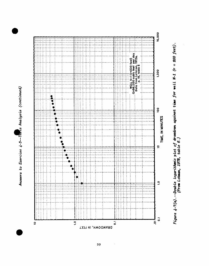
,.>.:...:..;..-1 . . ..I . . . . . . > . . . . . . . . . . .>.:..>.;..>...: . ...! .,....: . . . . . . . . . . . . i.!.;.+..:-..! . . . . F . . ...! . . . . . . . . . ..p.>.!..f . . . . . ...! . . . . . . 9s f.......... d..! ..,‘. :‘..;..a . . . . . . . . . . . < . . . . . . . . . . . . ~.~.!‘~..<...~ . . . . . . . . . . . . . . . . . . . .
~.-.:.‘..f...L...: . . . . . . :..... . . . . . . . . l . . ...! . . . . . . . . . . . . _.._..: . . . . . . . . . . . . . . . . . . . . . . . p . . . . . . . . . . . . . . . . . . . . . . .
. .:_ :. . I . . . . . . * * .
.,-..‘..-.i......i-...........(.i.~..:..-~..(....~..-..i......-.....;.).1-.:...:...I...“......)........ :::.: , . . . . . . . : .
“~‘~‘~“~...~...~ . . . . ..-.......... . ...:
.:‘<..:‘.;..;...~ . . . . . . . . . . . . . . . . . . . . . . . . ~~:.~..:‘..~.“:....~ . . . . . . . . . . .._..
: . . ..; . . . . . ;..;...y . . . . . . . . . . . . . . . . . . . . . . ..i .,.. :..:...:...; . . . . . . . . . ..I . . . . _ . . . . . . .;.> .,‘.,.‘&..;.- ..I......; . . . . . . . . .‘:: ’
.:::. : f :“: . . : :
: : : “:: : . .
.,..:..;..:...:-...: . . . . . . . . . . . . . . _ . . . . . . . . . . . :...: . . . . . . . . . . . . . . . . . . . . _ . . . . . ’ . . . . . . . :.;..:... E
.:;:I ; ::::: : : ‘.i’ :
~ d .j .,.......
. .
:.:., . : : “::: : . :.:: : QLN :
. . 0 e6 _.:._: ..,..: . . . . . . . . . . . . . . . . . . . . . . . . . . . . ;...;..:..: . . . . . . . . . . . . . . . . . . . . . . . . . . . +..j..j...~ ac .i . . . . . . . . .
,:::: : . . . .
. : :
.:::: 1 : : :‘: ,
. : . ..:: . .
: : ‘.: : .: . ‘. : :
: ..;:: : : : .
: f : ,: i:: : . : : :
.:: . a.: . . . . * *
. . . . .
; $g$
.
..:..:..i..i-.-~.-.; _.__._ ~ .._._._I_. .~~.~.~~~~:~~~:~..~....~~..~.~~.~..~-..~..;~~.;.~~.~.:--. &.2’0-
.d..: . . . . . F..” . ...! . . . . ..*............I. 1 .L.. > . . . ...! . . . . . . . . . . < . . .._.__._
*a ..< .-.......
. . . .:...\ _a._ <...- 2 Q) . . . . . . . . . . .
_.:__:_ . . . . t...: . ...! . . . . . . :_ . . . . . . . . . ..a. 8 . . . . I ..C..! . . . . . . . . . . $ . . . . . . . . . . . . .
..;..y
. . . *
.,..I . ...) . . . . . . . . . . . . . . . . . . . <.;.<..:...>..; . . . . . . . . . . . ;..-- . . . . . .
.!...‘..... :... . . .
.;.>.:..<...:...
& 0 E’.i . . . . . .._.
:.: .
0 0 &.i . . . . . . . . .
. ..a.. . . ..*, 1 -Jo* ..:‘.:‘.~‘.~‘~ . . . . . . . . . . . . . . . . . . . . . . . . . . :.:.:..: . ..“‘! . . . . . . . . . . . . . . . ..f..... :.:.: ‘d,.. <...w
--1O . . . . . . . . . . .
.:: : :.: . .*:. . ..; ..;.: :..,....I . . . . . . . . . . . . . . . . . . . . . . . . . . .!..; ..,... i...; .-., i . . . . . . . . . . . . . . . . . . ;.:..z..;..:... p&E :
:::: :
..:..:..;..;...: . . . . . . . . . . . . . . . . . . . . . . . . i.: .,.. :..: . . . . . . . . i..- . . . . . . . . . . . . . . . :.;..-.: . . . . . .
: . : ::;: f . . . . *
“: *
wx .; . . . . . . . .
.; . . ..-....
,:: ;
bi :
.:::: : :
Q
..;..;.;..i...+ . . . . . . :, . . . . . . . . . . . j.i..i..i..i..i . . . . j . . . . !
ii::: : :
. ::::: i . . . *
f . . . . . . . . . . . . . . . , . . . -:. . .,. . . . . . . . . . . . . *, . . _ - f . f f
: : : i ..::: : : . *
:.::: : a . : .:::. * : *.:::: . * . .
,:. ::I: . : : i :
.:::: : . “::: : ..:. * : : : :::. .
::..: : : .* : : * . . . .
;..:..:..i..;...: . . . . . . . . . . . > . . . . . . . . . . .:.;. .I. .:. . .:. ..;. . ..f . . . . . . . . . . . . _... .;.>.;.,...:...: . . . . . . . . . . . > . . . . ..-. ~.:.:.:..!...:....:......:*..-....:.:.-:.-:..!.-:-..:-..,!.-..-.:.-....-...:-!.!.!.-:-..1--i..-.:--.-..!-.-..... :_ _._. :_ .._.! _.......! _....................~ . . . . . . . . . . . . . . . . . . . . . <a . . . . . . . . . . . !.:.f.‘..‘...; . . . . > . . . . . :..-..-” +:..:..(...f . . . . . . . . ...) ;..* . . . . . . . +~..+.i . . . . i.- . . ..I . . . . . . . . . . . . j.iej..i’.‘>..; . . . . . . . . . . . I . . . . . . . . F.l..+;...; . . . . i . . . . . . . . . . . l . . . . . . :.; *..._ . ..*..: . . . . . . . -..<- . . . . . . . . . . f...! .I.. <...i . . . . . .,.......... _.. : :’
; : . i.i.~..~..~...+~ . . . . . . . . . . . . * . . . . ;.<..:..I..;...; . . . . i . . . . . . i . . . . . . . . . . . . ;.; : ; .q.....: . . . . . . . . . . . . . . . ‘........
: : ++;...; . . . . . . . . . . . . . . . . . . . . ..-i.i....+.: . . . . . . . . . . . . . . . . . . . . . .
.. : . ; ; 1
0 0 -T ; 0 b .
133 NI ‘NMOaMVtlCl
99

::;:: :
.. . .... .;. . , ............
: : :‘i: i
. .:. .:. . ; : : :
.....
.::
.:. ... , ...
...
.:::: :
.:: . .... .
. . .:. . . . . . . . .
: : : : : .
..:..:..i-.i--.~..-i----.-:-...--.--
. a. .:. . . . . . ,..: . ...! . . . . . . . . . . . . . . . .
__:_ _._. . . . , . . . . . . . . !. . . . . _:. . . . . . . . .
..:..i--I..i...:-...: . . . . . . . . . . . . . . . .
- -‘- -i- .
. . . . . . . . . . . . . . . . .._.............
. :: ::. ..:..:..i..;...: . . . . . . . . . . . > . . . . . . . .
.:::: .
..:..:..;..:...: . . . . . . . . . . . . . . . . . ..-. .::: : : : b : ..&Li...; . . . . . $....‘........, : : : : .:: : s.1: : :.: : jo :
: :oi .:..: . . ..:..)..:..;...~...; .I....? . . . . . . . . ,__:__:_ _,_. :...;...:...*; . . . . .._.
,* . . . . ..::: : . ,. . , . .; . . . . . . .. . . . . .:::: .
. . . . . . +..-...
, : : : : : 0 ..:..:..;..:.-.: . . . . ..__.... . . . . . . . . . . .:: .:.:: : : 0
: : : : : 0 ,.:.* . . _.... . . 0
I . . . . .
. .
. .
.,.
. .
. . .
. .
. . .
. . .
. . .
..,
. . .
. . .
1..
..,
. . . . .
._,
. . .
. .
. .
.
. . .
b- . . .
4) . . .
. .
. . .
. .
.._
..,
. . . . .
. .
. . .
. .
. . .
. .
. . .
i
““: : : . :..>.:...;..;...> . . . . . . . . . . . f . . . . . . . . .__.._._....! _._.....! . . . . . . y . . . . . . . . ,,.. . : . .._ :.a.., . . . . . . . ..I . . . . . . . . . . . . . . 1. .j. _:. ! . . ) . . _;. . . . I.. . . . j.. . . . . . . ; . .._... z..;...:...; _.....-........ :(‘.:’ . :_ .~ .‘:. i _. , . . .i.. . i. - -
. . . . . . . .i.. . . . . . -
..,., . :.:..:..:..;...: . . . . . . . . . . . . . . . . . . . . .
.,“. . : ::: : : :
:
. ..__. 1....: . . . . . . :.. -.....
..: ... . .... >. .... . ........
.;. ... . ...... . ........
.;.... . . . ..............
0 ; d
133A NI ‘NMOCIMVW
100

; .:. .: . .:. . ; .. .> ... .:. ........ ; ... L .... >:.f.:..: ..:.
... ; ...... ; .... .......
... .
> ............
.:.:..~I..:......:- . ..-. ........ ......... ::.:.“.? .S...!.
p.:.:.!..;
:.>:.;.: ..:. ...... . ;.::z.r: . ,..‘..i-...) .....
::.:-_ ..!. ........
....... ‘:. ........ . ..!. ........... :.:y.:.:. ..... . ............
.........
.... .:.
.> >.‘...:. ........
:.r . ..r
..........
.: I : .; ..<. ... (..--. .... .....
:.f.>.>.:.-.: ... . .... . ..!
,: !<.? ... ...!
:-. ...... ....
............ ......
..<.; .<. .
f. ............. :.!.;..;..:...: ... .
:-.:. . .. . ........ *. .... ........ ~: ..~..~ . . . ....... y:y.:.y
..... : .
..........
.:.:. : : .... .......... . .............. :..: .......... . ..........

Answers to EATcisc (4-S) (continued)
Analysis of plot of 8 against t
Data from Lohman (1972a, p. 19, table 6)--Well N-3 (r = 800 ft);
Q = 96,000 fta/d
Match point 1
W(u) = 1.0; - = 1.0; s = 0.58 ft; t = 3.55 min U
3.55 t i --s-w = 2.465 x lo-* d
1,440
QWu) 96,000 ftrId l 1.0 (1) T s --w-m_ r -_-------_-____-_- = 13,170 ft*/d
4ns 4 l fr l .58 ft
Lehman's values: s = 0.56 ft, T = 13,700 ft*/d
(2) 1 4Tt - P --- U rs S
4Ttu 4 l 13,200 ft4/d l 2.465 x lo-' d l 1 S = e--w z ------------------------------------- = 2.03 x 10" M 2 x 10"
rs (800)4 ft*
Lehman's value: S = 2 x 10"
102

.
>.i..:..!..; >.i..:..!..; ... ... . . .... .... . . ................. ................. ’ f ’ f j..;..;..;..; j..;..;..;..; i.. i..
i i ... ... i.. i.. ...... ......
.... .... ... ... . . .... ....
:::; : :::; : :..:..:..;..: ‘.;..+; :::: : ... ... . . m m
.... .... i.. i.. .... .... :.a.. ..... .... ..:i: : :
i.. . . .... . : :::: : ::::. : : : .. ; m I D .::: : : i ::: .: : 4
: . :- .> .:. . ! . . . : l - ,...:...-i......~........ by..: . ...! . . . . . . . . . . . . ..-..... _ :_ .I........ t...: . ...! . . . . . . . . . . . . . n . . :.<..:..:..:...: . ...) . . . . . , (.... . . . . 4 _. :_ . . . . . . . . . . t...: . ...! . . . . . . . . . . . . . . . .
. .
i.;.;..)..: . .._.... i . . . . . < .I.. _ . . . . : :
.‘I:’ : : : : ..-...:..;..*...; . . . . . . . . . . . . . . . . . . . . .
:::: :
::::: ; i
:-;.:..‘..‘..: . . ..-...... :- . . . . . . . . . . . . . . . -..:. : :
:::: : : : . . . . . ..:;: : : ::... : .
;.>.;..;..; . ..-..... . . . ...! . . . . . . . . . y _:.. > .,.. :...: . . f . . . . . . . . . . . . . . . . b....? .,.. t...;...: . . . . .._......... :..)..:..t..;...: . . . . <......: . . . . . . . . .
0
:..:..>.;..f..‘....! ...... . .......... ..‘.a..‘..- ............. ......
. ..........
.. . ..... !.e. .. . ...........
...... . ..........
:.;.<..:...> ..a.. ... I.. .... . .......... . . . .a,,-. ... :..: ..I.. . .: ...... . .......... :*:.:: : :.:..:..:..+ ..<. ... >. .... :. ......... ....... .
::“: : : ,.... :..: ..,...,..,.,...... . . . . . . . . . . . . . . . * :::: :
. : : “.:. :.: .,.._......; . . . . . . . . . . . . . . . . . . . . . . . . , .
::::’ : .., . :
i
:::: : : :
:::: : : .
,*... : :
:.;..:..:...: . . . . I... .> . . . . . .I . . . . . . . . . :.:.:‘.:..y..: . . . . . . . . ...! . . . . . . . . .
‘.a.‘..! ..C.............< . . . . . . . . . . I
!.,.!..:..,...! . . . . . . . . . . . i . . . . . . . . . . . . . . ..A . . . . ., ..-._I . . . .._..... _ . . . . . . . . ,:::: : . ; i.:..:..:...:...; . . . . . . . . . . . . . . . . . . . . .
: : :.::: : : :.; .\.. ;..:.. ..: . . . . . . . . . . . . . . . . . . . .
.;;i: : :
::::: : : : . . . . . . . . . . ;...: . . . . . . . . . . . . . . . . . . . . .
a., , :::.
: : : .:::. * *
: : :‘:” : . . . .
: : :
i.;.:..:...: . ..!. ... . ...... . .........
:.<.*... ................. 2 .....
..........
:.:.: ..‘.- .a ............... . ......... ...
>.:..>.;..!...>...f . . . . . . . . . . . . . . . . . . . . . . , * ..!.‘.-‘..e...............,.........
:.’ : : i.;.t..J..~..< . . . . . . . . . . . . . . . . . . . . . ::::. : : . . ;.e.r.v...:...; . . . . . . . . . . . . . . . . . . . . . ::::: : : :::.:: : ;.:.;.:..;...; . . . . :...-..; _........ . . . . . . . ..::: : : ..::: : : .:::: : f ; .*... . ...* . . . :.;.:.-:...:-..+ . .._ >.-...; . . . . . . . . . ~.~.~..~...........~......!.-.......
:.:.:.;..;...i . . . . i . . . . . . . . . . . . . . . . . , : : : . . . ::; ; . : . . . . . . . . . : : : : : . L; ; I..;..;..;..:
...... ... .
..I.. . .. . .:.a..: .:_ .; ..> .;.
..a.. .................
.... ........
.;. ....
...... ..!.
... * .... ..; ......... ;.1.; ..i .............. m ..... i.y.$~ . ..i.. .. . ...... . ......... : : . :. ,,.:.,, UI ..‘. ... . ...... . .......... :.;*.~~~ I 1 i : =~ ..‘.... i ..... . ......... : :
“‘.:i : : : . :.:.: ._-_. ‘...Z . . . . . . . . . . . . . . . . . . . . _ : : . :;: : ; ::: : ::: . ::: : : : .__: t:
i.!.;..:...:...‘......... -2 . ..-..... :.;.*.A.:...; . . . . . . . . . . . . . . . . . . . . *.* 9 I..., . . . . . . :_ . . . . . . . . . . . . . . . . . . . . . . . * . . * * ;.>.;.A..:...% . . . . . . . ..-.......... . . . . . . : : ;.;.:..y ..F ..: .... . ..... . ......... :. : * :.t.,.+..~ . ..[. ... . ...... . ........ ::::: : . i.;.:..:...: . ..t.. .. . ..... .1.........
::::: : : *
*.::: : . *
:
..::;. :
. .
. . . . 1 :
::::: : :. .:. .: .; . . : . _ .:. . . . . . , . . . . . ..::: : . .
::: : : .-- .; : ,:..:.;..:..:. * ..i........
0 ,’ d z .
13311 NI ‘NMOClMVtla
103

Answers to Exercise (4-S) (continued)
Analysis of plot of s against t/r2
Data from Lohman (1972a, p. 19, table 6)--selected drawdown data for wells
N-l, N-2, N-3; Q = 96,000 ft'/d
Match point 1
W(u) = 1.0; - = 1.0; 8 = 0.57 ft; t/r2 = 5.1 x 10s6 min/ft* U
Q.W(u) 96,000 ftaId x 1.0 (1) T = ---v-v = ---------------w-- = 13,400 ftg/d
4?rs 4% x .57 ft
(Lehman's value: T = 13,700 f@/d)
(2) 1 4Tt - I w-w z 1.0 U rs S
tu ftnId 1 d min. 1 S I 4T ..- = 4 x 13,400 ----- ----- ---w x 5.1 x 10" --w---w = 1.90 x 10"
rq day 1,440 min ftl
(Lehman's value: S = 2 x 10")
104

0 Concept of Superposition and its Application to Well-Hydraulic Problems
Assignments
*Study Fetter (1988), p. 201-204; Freeze and Cherry (1979), p. 327-332; or Todd (1980), p. 139-149.
*Study Note (4-5)--Application of superposition to well-hydraulic problems.
*Work Exercise (4-C)--Superposition of drawdowns caused by a pumped well on the pre-existing head distribution in an area1 flow system.
Superposition is a concept that has many applications to ground-water hydrology as well as to other physical systems that are described by linear differential equations. We use superposition when we analyze (most) aquifer tests, perhaps without realizing this fact, and in the theory of images and image wells. Superposition also has applications to the numerical simulation of ground-water systems, a topic that is not discussed in this course.
Reference
Reilly, Franke, and Bennett (1987)
Comments
A comprehensive overview of the principle of superposition is provided by Reilly and others (1987a). Todd (1980) offers a thorough review of image-well theory, which is a first-priority extension of this course on the topics of superposition and radial flow because it deals with the effects of hydrogeologlc boundaries on the drawdown response of water levels to a pumped well.
105
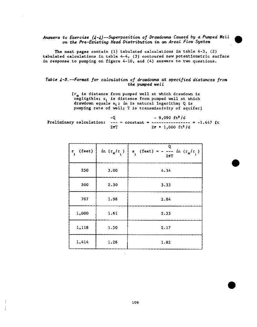
Answers to Exercise (d-4)--Superposition of Drw&ums Caused by a Pumped We1 1 on the Pm-Existing Head Distribution in an Area1 Flow System
The next pages contain (1) tabulated calculations in table 4-3, (2) tabulated calculations in table 4-4, (3) contoured new potentiometric surface in response to pumping on figure 4-10, and (4) answers to two questions.
Table 4-S. --Format for calculation of drawdowns at specified distances from the pumped well
[re is distance from pumped well at which drawdown is negligible; rI is distance from pumped well at which drawdown equals sl; In is natural logarithm; Q is pumping rate of well; T is transmissivity of aquifer]
-Q - 9,090 ftsId Preliminary calculation: --- = constant = ---------------- = -1.447 ft
2aT 2~ ' 1,000 ftlld
1 fi (feet) / In (fe/f, 1
I 250 I
3.00
) 500 / 2.30
1,000 1.61
1,118 1.50
1,414 1.26
s1 (feet) = - -Q- In (re/rl) 2nT
4.34
3.33
2.84
2.33
2.17
1.82
106

Ansums to Exercise (4-4) (continued)
Table 4-4. --Format for calculation of absolute heads at specified referemcr poht8
107

Answers to Exercise (d-4) (continued)
EXPLANATION -Ii?- HEAD CONTOUR, IN FEET 0 LOCATION OF PUMPED WELL
-- - SYMMETRY LINE FOR HEAD CONTOURS OF REFERENCE POINT WITH
all.16 HEAD AT REFERENCE POINT, IN FEET WELL IDENTIFIER
Figure d-10. --Head distribution in confined area1 flow system resulting from pwnjpiw. l
108

Ansu~crs to Exercise (I-4) (continued)
Question (1). The first two streamlines drawn on figure 4-10 represent a type of ground-water divide that is analogous to the hydrologic situation depicted in figure 3-35, Exercise (3-3). Between these two bounding streamlines, all streamlines in the aquifer terminate at the pumped well. Outside the area bounded by these two streamlines, all streamlines in the aquifer continue to flow downgradient beyond the well as part of the regional flow system. The area between the two bounding streamlines is called the area of diversion of the pumped well.
Consider the steady-state, three-dimensional configuration of potential surfaces and related streamlines that are found in a ground-water system in equilibrium with a single pumped well. Conceptually trace upgradient all the streamlines that terminate at the pumped well to their point of entry into the saturated ground-water system. In real systems, this point of entry is generally at the water table or at the bottom or bank of a surface-water body. The shape of the volume of saturated earth material that is defined by this "bundle" of streamlines can be c&plex, particularly for wells screened near the bottom of thick unconfined aquifers or in confined aquifers between leaky confining units.
The term "contributing area" usually is used to define the area through which water enters the ground-water system and is synonymous with the term "recharge area." Thus, this area constitutes the starting points for the "bundle" of streamlines that enter the ground-water system through a boundary surface. The area of diversion, however, is the projected area in map view of the entire bundle of streamlines as they flow to their point of discharge at
0 the well.
In terms of the class problem under discussion, it is useful, as always, to review its boundary conditions and impliclt assumptions--(l) the pumped well is screened in a confined aquifer; thus, the saturated thickness of the pumped aquifer is assumed to remain constant; (2) the analysis is done with the assumption of two-dimensional flow in plan view; this assumption is best approximated in real systems if the pumped well completely penetrates the confined aquifer; and (3) the source of water to the regional flow system before pumping and to the pumped system is a plane constant-head boundary located at a great distance upgradient from the pumped well; no water enters this system by leakage through an overlying or underlying confining unit.
The area of diversion in the class problem, therefore, is the surface projection of the area encompassed by the two bounding flow lines drawn on figure 4-10. The location of the recharge area or contributing area depends on the actual source of water entering the ground-water system. This source of water is not explicitly stated in our problem; however, because the equipotential lines in the undisturbed system are evenly spaced, we can assume, as stated above, that there is no local source of water entering the system and the source of water ast be an upgradient-plane constant-head boundary. The contributing or recharge area can not be defined for the class problem as given, and it would exist beyond the area shown in figure 4-10.
109
The existing terminology as used in many reports for terms such as zone of contribution, contributing area, and area of diversion is frequently confusing because it is based on two-dimensional systems, and it is imprecisely defined' for three-dimensional systems. In three-dimensional systems it is desirable to identify the volume of earth material and contained fluid that is associated with flow to a pumped well, and to envision the changing shape of the actual "bundle" of flow tubes that constitute this volume from its entry into the flow system to its discharge from the system at the well. This conceptualization should be clearly explained in reports, instead of relying on terminology that Is frequently misleading.
Question (2). The purpose of this question is to emphasize the difference between the area of diversion of the pumped well and the area of influence of the pumped well. Theoretically, the area of influence of the pumped well extends to the aquifer boundaries; in a practical sense, however, we can define the area of influence as the area of the aquifer in which we can measure drawdowns resulting from the influence of the pumped well that are greater than _ or equal to 0.01 ft. Our calculated data and contour map (fig. 4-10) show that (1) the ground-water divide between the tw "areas" exists between reference points S, T, X, and Y and the pumped well; and (2) quantitatively significant drawdowns, as exemplified by the calculated drawdowns at these four points, are found inside the area of influence but outside the area of diversion of the pumped well.
110

Aquifer Tests
0 Assignments
*Study Fetter (1988), p. 204-209; Freeze and Cherry (1979), p. 335-343, 349-350; or Todd (1980), p. 45-46, 70-78.
*Study Note (4-6)--Aquifer tests.
One of the main activities of ground-water hydrologists is to estimate physically reasonable values of aquifer parameters for different parts of the ground-water system under study. The most powerful and direct field method for obtaining aquifer parameters is a carefully designed, executed, and analyzed aquifer test. Unfortunately, aquifer tests are labor- and time-intensive. Often, the most important decision concerning an aquifer test is whether or not to perform one-- in other words, whether the value of the test results equals the cost of obtaining those data. This question generally is difficult to answer.
References
Heath and Trainer (1968), p. 83-84, 119-127. Lohman (1972a), p. 52-54. Stallman (1971).
Comments
0 Our goal in this subsection is to initiate a discussion of aquifer tests-- what they are and what we seek to accomplish by undertaking them, their advan- tages and disadvantages, and their implementation in three phases--design, field measurements, and data analysis. In addition, adequate information is available in the keyed course textbooks and other listed references for a dis- cussion of other ways in which hydrogeologists estimate aquifer and confining- unit coefficients. Introduction of this information is appropriate at this time.
111

SECTION (6).-GROUND-WATER CONTAMINATION
The goal of this section of the course is to introduce the physical * mechanisms of solute movement in ground water. Further treatment of the vast and rapidly developing area of science and technology related to ground-water contamination can be found in the extensive literature that is available or in additional training courses.
Background and Field Procedures Related to Ground-Water Contamimtion
Assignments
*Study Fetter (1988), p. 367-389, 406-442; Freeze and Cherry (1979), p. 384-457; or Todd (1980), p. 344-346.
The depth of topical coverage in this section of the course will depend primarily on the time available and the interests of the instructors and participants. A useful and readable discussion on the conceptualieation and organization of a field study involving solute transport, along with a pertinent bibliography, is provided by Reilly and others (1987).
Reference
Reilly, Franke, Buxton, and Bennett (1987)
Comments
The focus of this course is hydrogeology and the hydraulics of ground- water flow. A section on ground-water contamination is included primarily because of its present-day topical interest. The keyed course textbooks and the reference above provide much more information on ground-water contamina- tion than can be discussed in this course. Freeze and Cherry (1979, pa 384- 401) provide a thorough introduction to the physical mechanisms of solute transport.
112
Physical Mechanisms of Solute Transport in Ground Water
a Assignments
*Study Fetter (1988), p. 389-405.
*Study Note (S-1)--Physical mechanisms of solute transport in ground water
*Work Exercise (S-1)--Ground-water travel times in the flow system beneath a partially penetrating impermeable wall
*Work Exercise (S-2)--Advective movement and travel times in a hypothetical stream-aquifer system
*Study Note (S-2)--Analytical solutions for analysis of solute transport in ground water
*Work Exercise (S-3)--Application of the one-dimensional advective-dispersive equation
The background for this section is provided in Note (S-l), which is an introductory discussion of the basic physical mechanisms of solute movement-- advection and dispersion. Exercises (5-l) and (5-2) consider only advective movement of ground water and involve calculation of travel times by using the average linear velocity (Darcy velocity divided by porosity). In Exercise (S-l), travel times are calculated in a vertical section of a simple flow system; in Exercise (S-2), travel times are calculated in plan view.
0 Comments on the field application of analytical solutions to the advective-dispersive differential equation are provided in Note (S-2), and Exercise (5-3) involves numerical calculations with one of the simplest analytical solutions.
113

Answers to Eizemise (5-1)--Qrowad-Water Travel Times in the Flow System Beneath a Padially Penetrating Impermeable Wall ,@
With reference to the plotted time-of-travel values (as calculated in table 5-1) and related equal-time contours in figure 5-5, the total time of travel from the recharge boundary to the discharge boundary along the longest bounding streamline is about 20 times greater than the total travel time along the shortest bounding streamline around the impermeable wall. The time of travel for increments of the longest streamline vary widely. The longest travel times per unit length of streamline are found in the lower left-hand corner, in‘the lower right-hand corner, and at the right-hand vertical boundary. This observation is predictable from the low head gradients in these regions. The shortest times of travel in this system are found beneath the impermeable wall, where head gradients are greatest.
Hydrologists are not accustomed to calculating time-of-travel contours and visualizing their general pattern in ground-water systems. The pattern of these contours does not bear a visually obvious relation to the more familiar head contours and streamlines. Because of the present-day prevalence of contamination studies and the advent of particle-tracking algorithms in association with digital flow models, we can expect ever-increasing applications of time contours and "surfaces" in ground-water studies.
114

115

Answers to Exercise (5-l) (continued)
Table 5-l .--Fomat for calculation of time of travel along selected flowlines in impemeab Le-wall problem (page 1 of 3)
[h is head at a node or other point in flow system; L is distance between two @oints on a flowline at which head is known; Ah is difference in head between two points on a flowline; t is time of travel between two points on a flowline; Ct is time of travel from inflow boundary to point on flowline; 9 is stream function)
t (days) =
h L Ah 6.67 x 10" Lp Et --------------
(feet) (feet) (feet) Ah ( daya 1
Flowline 55.00 (a) 9 54.25 g 0 = 53.52
52.81 52.16
-- em
5.0 0.75 5.0 .73 5.0 .71 5.0 .65
-a -w
0.223 0.223 .229 .452 .235 .687 .257 .944
51.54 5.0 .62 .269 1.213 51.03 5.0 .51 .327 1.54 SO.62 5.0 .41 .407 1.947 50.33 5.0 .29 .576 2.523 50.19 5.0 .14 1.193 3.716
50.08 5.0 .ll 1.518 5.234 49.97 5.0 .ll 1.518 6.752 49.66 5.0 .31 .539 7.291 49.31 5.0 .35 .477 7.768 48.80 5.0 .51 .327 8.095
48.10 5.0 .70 .239 8.334 47.15 5.0 .95 .176. 8.510 45.90 5.0 1.25 .134 8.6.44 44.24 5.0 1.66 .lOl 8.745 42.02 5.0 2.22 ,075 8.820
39.13 5.0 2.89 .058 8.878 35.68 5.0 3.45 .048 8.926 32.83 5.0 2.85 .059 8.985 30.71 5.0 2.12 .079 9.064 29.17 5.0 1.54 .108 9.172
28.07 5.0 1.10 .152 9.324 27.28 5.0 .79 .211 9.535 26.73 5.0 .55 .304 9.839 26.35 5.0 .38 .439 10.278 26.10 5.0 .25 .668 10.946
116

0 Answers to Exercise (5-l) (continued)
Table 5-1 .--Format for calculation of time of travel along selected flowlines in impermeable-wall problem (page 8 of 3)
0
t (days) =
h L Ah 6.67 x 10'" Lp Et --------------
(feet) (feet) (feet) Ah (days 1
25.96 5.0 0.14 1.193 12.139 25.90 5.0 .06 2.783 14.922 25.87 5.0 .03 5.567 20.489 25.74 5.0 .13 1.285 21.774 25.54 5.0 .20 .835 22.609
25.28 5.0 25.00 5.0
Flowline 55.00 5.0 -- -- (f) 9 53.88 5.0 1.12 .149
Q = 1.0 52.75 5.0 1.13 .148 51.56 5.0 1.19 . 140 50.28 5.0 1.28 .130
48.84 5.0 1.44 .116 .683 47.11 5.0 1.73 .097 .780 44.77 5.0 2.34 .071 .851 40.77 5.0 4.00 .042 .893 33.97 5.0 6.80 .025 .918
29.80 5.0 27.17 5.0 25.00 5.0
.26
.28 30.00
4.17 2.63 2.17
30.00
.642 23.251
.596 23.847
.040 .958
.063 1.021
.077 1.098
-- .149 .297 .437 .567
117
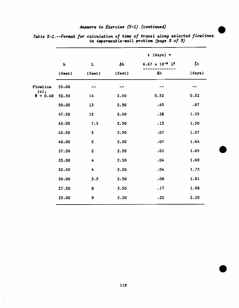
Answers to Exercise (5-l) (continued) @
Tcrble 5-l.. --Fond for calculation of time of travel along selected flowlines, in impermeable-wall problem (page 3 of 3)
t (days) =
h L Ah 6.67 x 10" L" Ct --------------
(feet) (feet) (feet) Ah (days)
Flowline 55.00
1%.40 52.50
50.00
47.50
45.00
42.50
40.00
37.50
35.00
32.50
30.00
27.50
25.00
-- --
14 2.50
13 2.50
12 2.50
7.5 2.50
5 2.50
5 2.50
2 2.50
4 2.50
4 2.50
5.5 2.50
8 2.50
9 2.50
0.52
.45
.38
.15
.07
.07
.Ol
.04
.04
.08
.17
.22
--
0.52
.97
1.35
1.50
1.57
1.64
1.65
1.69
1.73
1.81
1.98
2.20
118

An.swers to Exercise (5-Z) --Advectivc Movement Md Trave 1 Times in a Hypothetical Stream-Aquifer System,
I. For Point A (as shown on figure 5-6):
1. Length:
La = 1.65 mi = 8,712 ft
2. Velocity:
K dh 125 ft/d 16 ft lmi VA = - -- =
-;;-
l ------- 0 -------- = 0.70 ft/d n dl 1.65 mi 5,280 ft
3. Time of travel:
LA 8,712 ft tA = -- =: --------- = 12,446 d = 34.1 yr
VA 0.70 ft/d
II. For Point B (as shown on figure 5-6):
1. Length:
LB = 2.90 mi = 15,312 ft
2. Velocity:
125 ftld 26 ft lmi VB =
--:;;--
l ------- 0 -------- = 0.64 ft/d 2.90 mi 5,280 ft
3. Time of travel:
LB 15,312 ft tB = -- = ----e---w t 23,925 d = 65.5 yr
VB 0.64 ft/d
Comment: Estimates of travel time based on water-table maps and available estimates of hydraulic conductivity are simple to calculate, require minimal time, and provide an approximate but generally reliable frame of reference for travel time that is the foundation of any investigation involving ground-water contamination.
119

Answers to Ezercisc (5-B) (continued)
EXPLANATION
-2o- WATER-TABLE CONTOUR -- Shows altitude- of water table. Contour Interval 10 feet. Datum is se’a level
0 41 LOCATION OF START-OF-FLOW OF STREAM -- Number is altitude of stream. in feet above sea level
A* LOCATION AND NUMBER OF STREAM-DISCHARGE MEASUREMENT POINT
Figure 5-6.--Hypothetical rater-table map of an area underlain by pemeabh &posits in a huanid climate showing streamlines from point A to strem B and from point B to stream A. l
120

Anscoers to Exercise (5-9)--AppLication of the One-DimensionaL
a Advection-Dispersion Equation
The following pages contain calculations of concentration as a function of distance from the source in tables 5-2 and 5-3, and a plot of these data in figure 5-9.
The curves in figure 5-9, based on the calculations in tables 5-2 and 5-3, provide a visual summary of classical advection-dispersion theory and the role of the dispersion coefficient. The frame of reference is the vertical line representing a "sharp front" between contaminated and uncontaminated ground water at a distance, L = 2,000 ft, from the contaminant source. The existence of a sharp front implies pure advective transport, or no mixing across the front.
The principal reference point on the vertical sharp front line is the point at which the relative concentration C/C, = 0.50. Curves of relative concentration for dispersion coefficients are symmetrical about this point for conditions where the simplified equation (3) is valid (i.e. the dispersion coefficient is small, or the distance is far from the boundary, or the time is large). For smaller coefficients of dispersion, at a given time and distance from the source, the symmetrical mixing zone relative to the sharp-front reference line is relatively narrow. For larger dispersion coefficients, at a given time and distance from the source, the zone of mixing is broader and may extend to the contaminant source.
121

Answers to Eercise (5-3) (continued)
Tizble 5-a.--Format for calculating solute concentrations when the dispersion coefficient D = 10 square feet per day and the elapsed tinae t = 1,000 days
[d, days; it/d, feet per day; ftpId, square feet per day; mg/L, milligrams per liter]
Formula for
c =
Co = L = v = t = D = erfc :
Preliminary
% L - vt calculations: C = -- erfc ------
2 ( 1 where 2IE
concentration of solute at point in plume at specified time, in q/L solute concentration of source, in mg/L distance from source, in feet average linear velocity of ground water, in ft/d elapsed time since introduction of solute dispersion coefficient, in ft41d complementary error function (see Fetter,
at source, in d
1988, po 562)
calculation:
IL -vt, L - 2ftld l 1,000 d L- 2,000 For D = 10 ftrld, '-;;E-j 52 ------------------- I -----e-m-
2h0ft4/d l 1,000 d 200
L-2,000 L-2,000 1 L-2,000 L ------- erfc ( ----a-- > c= 50 mg/L erfc(-------)
(feet) 200 200 200 1,500 -2.5 1.999 100. mglL
1,600 -2.0 1.995 99.75 mg/L
1,700 -1.5 1.966 98.3 mg/L ~~
1,800 -1.0 1.8427 92.1 mg/L
1,900 - .5 1.5205 76.0 mg/L
2,000 0.0 1.000 50.0 mg/L
2,100 .5 .4795 24.0 mg/L
2,200 1.0 .1573 7.9 mglL
2,300 1.5 .0339 1.7 mg/L
2,400 2.0 .0047 .24 mg/L
l erfc(-x) = 1 + erf(x)
122

Answers to Ezcrcise (5-3) (continued)
Table 5-3.--Format for calculating solute concentrations when the dispersion coefficient D = 100 square feet per day and the elapsed time t = 1,000 days
[d, days; ftld, feet per day: ftn/d, feet squared per day; mg/L, milligrams per liter]
Formula for
C t
c, = L = v = t = D = erfc =
Preliminary
CO L - vt calculations: C = -- erfc ---,-
( > where 2 2dDt
concentration of solute at point in plume at specified time, in mg/L solute concentration of source, in mg/L distance from source, in feet average linear velocity of ground water, in ft/d elapsed time since introduction of solute at source, in days dispersion coefficient, in ft*/d complementary error function (see Fetter, 1988, p. 562)
calculation:
fL -vt, L - Pftld l 1,000 d .~ --_ For D = 100 ft'ld, [-;;& t ----w-v---------w-em
2~100ft'/d'. 1,000 d
L- 2,000 = -c-------
632.5
L-2,000 L-2,000 1 L ---m-m- erfc ---w--w
( 632.5 1 C = 50 mg/L erfc
(
L-2,000, -v----w
(feet) 632.5 632.5 '
1,000 -1.58 1.974 98.7 mg/L
1,250 -1.185 1.905 95.3 mg/L
1,500 - .791 1.736 86.8 lug/L
1,750 - .40 1.428 7.1.4 mg/L
2,000 0.0 1.000 50. WL
2,250 .40 0.572 28.6 mg/L
2,500 ,791 0.264 13.2 mg/L
2,750 1.185 0.095 4.75 mg/L
3,000 1.58 0.026 1.3 mg/L
l erfc(-x) = 1 + erf(x)
123
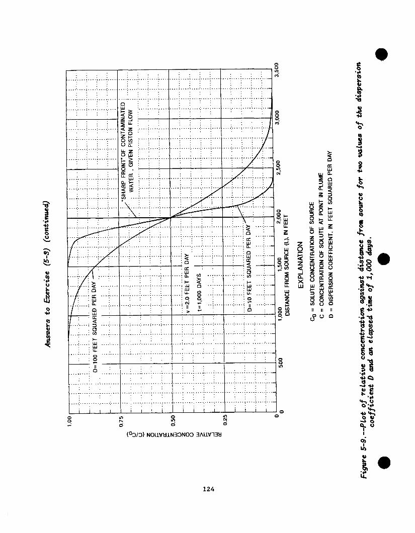
. ..I . . . . . . . . .._...__...._.......~ ._..:.__. :...- I_i:!- fs~~
Q z ; . . . . . . . . . i . . . . . . . . 1 . . . . :; . . . . i . . . . . . . . . . . . . i . . . . 1 . . . i . . . . i...
E & I . . . . . . . f . . . . ..‘..~ . . . . ;...; . . . . . . . . t . . . . :...: . . . . :...;./.y
un”: : : LL. z :....; . . . . - . . . . . . . . . 1 i.... f . . . . . . .._.; . . . . I...; . . . . j . . . . ;...q . OW L > ; . . . . f . . . . . . . . . I.... i . . . . :...: . . . . . . . . . I...: . . . . . . . . . y.; . ..” . .
: : : : .__........._... -... .
: : : ..: . . . . . . . . . . . . . . I...
: : : :
. . _. . . . . . . - . . . -. . .
: : :
: : :
. ., . . . . : . . ,. . . . ., . .
: :
.
: : : . . . . . . . . . . . . . . . . . . i...
: .._ . . . . . . . . . -........
: : . ,...: . . . . . . . .._......... : :
: . . . J
ia: i i 0
i? ” : 5:
La: : : ti ,_.._~...._.... c& : : Q z yj . . . . . . . . . 5 . ..j . . . . . . . . . i . . . .
: :
=L
. . . ........:....I.... . . .z . . . . :. : : : :
,,.. .y-z- ,/v-v. . I .\.
A$
: 8 -0+
: ,;!A
. . . . . . . . I . . . . :...:... : : .
. : : . _..” . . . . . . . . . e........
: : : :
._..: . . . . . . . . . j.. ..:...
: : :
_ _ ” . . . . . . . . . ” . . . -. . . : : :
_..; . . . i....; . . . . . ;... .
.Y ..___...__......_._............ . . . . . . : : :
! _.; ___...... I . . . . . . . . . . . . . . . . I : :a '
. . . . . . . . . . n ‘W . I
.....; ii ‘II ..i . . . . . . . . . . . . . . ‘;i . . . _:. . .
. : : ;, +- ; 10 : g;”
: : : : : : 00 : -‘
. . . . . . . . . . . . . . . . . . . . >... . . . . . . . . . . . . . . . . . :‘.... : : : : : : . _ . . . . . . . . . . . _...: . . . . :....l......... : 1 : I
. . ..I . . ..I . . . . . . . . . . :... : : I- . . . . . . . . . . . . .._... “...
.___.__._. __- . . . . . .
. ..__.__....._... -..
. . . ., . . . ., . . . ,. . .j . . . . i . . . . . . . . . . . . . i . . . . Ii I 1 i 11 11 1
: . . . . . +.; . . . . . . . . . . i...
: I I I I 0
0 s1 d P
d
(o,/,) NOllVkilN33N03 3AllVTlti
124
Bear, Jacob, 1972, Dynamics of fluids in porous media: New York, American Elsevier, 764 p.
1979, Hydraulics of groundwater: New York, McGraw-Hill Book Company, 569 p.
Bennett, G.D., 1976, Introduction to ground-water hydraulics: U.S. Geological Survey Techniques of Water-Resources Investigations, Book 3, Chapter B2, 172 p.
Bennett, G.D., and Giusti, E.V., 1971, Coastal ground-water flow near Ponce, Puerto Rico: U.S. Geological Survey Professional Paper 750-D, p. D206- D211.
Bennett, G.D., Reilly, T.E., and Hill, M.C., 1990, Technical training notes in ground-water hydrology--radial flow to a well: U.S. Geological Survey Water-Resources Investigations Report 89-4134, 83 p.
Bureau of Reclamation, 1977, Ground water manual: U.S. Department of the Interior, Bureau of Reclamation, 480 p.
Davis, S.N., 1969, Porosity and permeability of natural materials, chapter 2, p. 53-89, in Dewiest, R.J.M., ed., Flow through porous media: New York, Academic Press, 530 p.
0 Davis, S.N., and Dewiest, R.J.M., 1966, Hydrogeology: New York, John Wiley and Sons, 463 p.
Domenico, P.A., 1972, Concepts and models in groundwater hydrology: New York, McGraw-Hill Book Company, 405 p.
Ferris, J.G., Knowles, D.B., Brown, R.H., and Stallman, R.W., 1962, Theory of aquifer tests: U.S. Geological Survey Water-Supply Paper 1536-E, 174 p.
Fetter, C.W., 1988, Applied hydrogeology: Columbus, Ohio, Merrill Publishing Company, 592 p.
Franke, O.L., and Cohen, Philip, 1972, Regional rates of ground-water movement on Long Island, New York, in Geological Survey Research 1972: U.S. Geological Survey Professional Paper 800-C, p. C271-C277.
Franke, O.L., and McClymonds, N.E., 1972, Summary of the hydrologic situation on Long Island, New York, as a guide to water-management alternatives: U.S. Geological Survey Professional Paper 627-F, 59 p.
Franke, O.L., Reilly, T.E., and Bennett, G.D., 1987, Definition of boundary and initial conditions in the analysis of saturated ground-water flow systems--An introduction: U.S. Geological Survey Techniques of Water-Resources Investigations, Book 3, Chapter B5, 15 p.
125

SELECTED REFERENCES (Continued) 0
Franke, O.L., Reilly, T.E., Haefner, R.J., and Simmons, D.L., 1990, Study cx
guide for a beginning course in ground-water hydrology: Part I--Course participants: U.S. Geological Survey Open-File Report 90-183, 180 p.
Freeze, R.A., and Cherry, J.A., 1979, Groundwater: Englewood Cliffs, New Jersey, Prentice-Hall, Inc., 604 p.
Gelhar, L.W., and Axness, C.L., 1983, Three-dimensional stochastic analysis of macrodispersion in aquifers: Water Resources Research, v. 19, no. 1, p. 161-180.
Haeni, F.P., 1988, Application of seismic-refraction techniques to hydrologic studies: U.S. Geological Survey Techniques of Water-Resources Investigations, Book 2, Chapter D2, 86 p.
Harr, M.E., 1962, Groundwater and seepage: New York, McGraw-Hill Book Company, 315 p.
Heath, R.C., 1983, Basic ground-water hydrology: U.S. Geological Survey Water-Supply Paper 2220, 84 p.
1984, Ground-water regions of the United States: U.S. Geological Survey Water-Supply Paper 2242, 78 p.
Heath, R.C., and Trainer, F.W., 1968, Introduction to ground-water hydrology: New York, John Wiley and Sons, 284 p. e
Hem, J.D., 1985, Study and interpretation of the chemical characteristics of natural'watert U.S. Geological Survey Water-Supply Paper 2254, 264 p.
Javandel, I., Doughty, C., and Tsang, C.F., 1984, Groundwater transport-- Handbook of mathematical models: American Geophysical Union, Water Resources Monograph 10, 228 p.
Jorgensen, D.G., 1980, Relationships between basic soils-engineering equations and basic ground-water flow equations: U.S. Geological Survey Water-Supply Paper 2064, 40 p.
Keys, U.S., 1988, Borehole geophysics applied to ground-water hydrology: U.S. Geological Survey Open-File Report 87-539, 305 p.
Lohman, S. W., 1972a, Ground-water hydraulics: U.S. Geological Survey Professional Paper 708, 70 p.
Lohman, S.W., ed., 1972b, Definitions of selected ground-water terms-- Revisions and conceptual refinements: U.S. Geological Survey Water-Supply Paper 1988, 21 p.
McClymonds, N.E., and Franke, O.L., 1972, Water-transmitting properties of aquifers on Long Island, New York: U.S. Geological Survey Professional Paper 627-E, 24 p.
126

SELECTED REFERENCES (Continued)
McDonald, M.G., and Harbaugh, A.W., 1988, A modular three-dimensional finite- difference ground-water flow model: U.S. Geological Survey Techniques of Water-Resources Investigations, Book 6, Chapter Al, 576 p.
Meinzer, O.E., 1923, The occurrence of ground water in the United States: U.S. Geological Survey Water-Supply Paper 489, 321 p.
Mercado, A., 1967, The spreading pattern of injected water in a permeability stratifled aquifer, in Proceedings of the International Association of Scientific Hydrology Symposium, Haifa, Publication No. 72, p. 23-36.
1984, A note on micro and macrodispersion: Ground Water, V. 22, no. 6, p. 790-791.
Milne-Thompson, L.M., 1955, Theoretical hydrodynamicsr London, Macmillan & CO.) 632 p.
Nahrgang, Gunther, 1954, Zur Theorie des vollkonxaenen und unvollkommenen Brunnensr Berlin, Springer Verlag, 43 p.
Prickett, T.A., and Lonnquist, C.G., 1971, Selected digital computer techniques for groundwater resource evaluation: Champaign, Illinois, Illinois State Water Survey, Bulletin 55, 62 p.
Prince, K.R., Franke, O.L., and Reilly, T.E., 1988, Quantitative assessment of the shallow ground-water flow system associated with Connetquot Brook, Long Island, New York: U.S. Geological Survey Water-Supply Paper 2309, 28 p.
Rantz, S.E., 1982, Measurement and computation of streamflow: Volume 1. Measurement of stage and discharge: U.S. Geological Survey Water-Supply Paper 2175, 284 p.
Reed, J.E., 1980, Type curves for selected problems of flow to wells in confined aquifers: U.S. Geological Survey Techniques of Water-Resources Investigations, Book 3, Chapter B3, 106 p.
Reilly, T.E., Franke, O.L., and Bennett, G.D., 1987, The principle of super- position and its application in ground-water hydraulics: U.S. Geological Survey Techniques of Water-Resources Investigations, Book 3, Chapter B6, 28 p.
Reilly, T.E., Franke, O-L., Buxton, H.T., and Bennett, G.D., 1987, A conceptual framework for ground-water solute-transport studies with emphasis on physical mechanisms of solute movements U.S. Geological Survey Water-Resources Investigations Report 87-4191, 44 p.
Saffman, P.G., 1959, A theory of dispersion in a porous medium: Journal of Fluid Mechanics, v. 6, p. 321-349.
127
SELECTED REFERENCES (Continued)
Shuter, E., and Teasdale, W.E., 1989, Application of drilling, coring, and sampling techniques to test holes and wells: U.S. Geological Survey Techniques of Resources Investigations, Book 2, Chapter Fl, 97 p*
Skibitzke, H.E., and Robinson, G.M., 1963, Dispersion in ground water flowing through heterogeneous materials: U.S. Geological Survey Professional Paper 386-B, 3 p.
Stallman, R.W., 1971, Aquifer-test design, observation, and data analysis: U.S. Geological Survey Techniques of Water-Resources Investigations, Book 3, Chapter Bl, 26 p.
Sun, R.J., ed., 1986, Regional aquifer-system analysis program of the U.S. Geological Survey--Summary of projects, 1978-84: U.S. Geological Survey Circular 1002, 264 p.
Theis, C.V., 1940, The source of water derived from wells--Essential factors controlling the response of an aquifer to development: Civil Engineering Magazine, May 1940, p. 277-280 (U.S. Geological Survey Ground Water Note No. 34).
Todd, D.K., 1980, Ground-water hydrology: New York, John Wiley and Sons, 535 p.
U.S. Environmental Protection Agency,, 1987, Handbook of ground water: EPA/625/6-87/016, 212 p.
Wexler, E.J., 1989, Analytical solutions for one-, two-, and three-dimensional solute transport in ground-water systems with uniform flow: U.S. Geological Survey Open-File Report 89-56, 250 p.
Zohdy, A.A.R., Eaton, G.P. and Mabey, D.R., 1974, Application of surface geOphy8iC8 to ground-water investigationsr U.S. Geological Survey Techniques of Water-Re8OUrCe8 Investigations, Book 2, Chapter Dl, 116 p.
128