global migration in the 20th and 21st centuries: the

HAL Id: hal-01743799https://hal.archives-ouvertes.fr/hal-01743799

Submitted on 26 Mar 2018

HAL is a multi-disciplinary open accessarchive for the deposit and dissemination of sci-entific research documents, whether they are pub-lished or not. The documents may come fromteaching and research institutions in France orabroad, or from public or private research centers.

L’archive ouverte pluridisciplinaire HAL, estdestinée au dépôt et à la diffusion de documentsscientifiques de niveau recherche, publiés ou non,émanant des établissements d’enseignement et derecherche français ou étrangers, des laboratoirespublics ou privés.

Global Migration in the 20th and 21st Centuries: theUnstoppable Force of Demography

Thu Dao, Frédéric Docquier, Mathilde Maurel, Pierre Schaus

To cite this version:Thu Dao, Frédéric Docquier, Mathilde Maurel, Pierre Schaus. Global Migration in the 20th and 21stCenturies: the Unstoppable Force of Demography. 2018. �hal-01743799�

https://hal.archives-ouvertes.fr/hal-01743799

https://hal.archives-ouvertes.fr

fondation pour les études et recherches sur le développement international

LA F

ERD

I EST

UN

E FO

ND

ATIO

N R

ECO

NN

UE

D’U

TILI

TÉ P

UBL

IQU

E.

ELLE

MET

EN

ŒU

VRE

AV

EC L

’IDD

RI L

’INIT

IATI

VE

POU

R LE

DÉV

ELO

PPEM

ENT

ET L

A G

OU

VER

NA

NC

E M

ON

DIA

LE (I

DG

M).

ELLE

CO

ORD

ON

NE

LE L

ABE

X ID

GM

+ Q

UI L

’ASS

OC

IE A

U C

ERD

I ET

À L

’IDD

RI.

CET

TE P

UBL

ICAT

ION

A B

ÉNÉF

ICIÉ

D’U

NE

AID

E D

E L’

ÉTAT

FRA

NC

AIS

GÉR

ÉE P

AR

L’AN

R A

U T

ITRE

DU

PRO

GRA

MM

E «I

NV

ESTI

SSEM

ENTS

D’A

VEN

IR»

PORT

AN

T LA

RÉF

ÉREN

CE

«AN

R-10

-LA

BX-1

4-01

».

Global Migration in the 20th and 21st Centuries: the Unstoppable Force of Demography Thu Hien Dao | Frédéric Docquier Mathilde Maurel | Pierre Schaus

Thu Hien Dao, IRES, Université catholique de Louvain, Belgium - Department of Economics, University of Bielefeld, Germany. [email protected]

Frédéric Docquier, IRES, Université Catholique de Louvain, Belgium -FNRS, National Fund for Scientic Research, Belgium - FERDI, France. [email protected]

Mathilde Maurel, CES, Centre d’economie de la Sorbonne, Universite de Paris 1, France - FERDI, France. [email protected]

Pierre Schaus, Department of Computer Science & Engineering, Universite catholique de Louvain, Belgium. [email protected]

Abstract

This paper sheds light on the global migration patterns of the past 40 years, and produces migration projections for the 21st century, for two skill groups, and for all relevant pairs of countries. To do this, we build a simple model of the world economy, and we parameterize it to match the economic and socio-demographic characteristics of the world in the year 2010.

… /…Keywords: international migration, migration prospects, world economy, inequality.JEL codes: F22, F24, J11, J61, O15.

AknowledgmentWe thank Christiane Clemens, Giuseppe de Arcangelis, Timothy Hatton, Vincent Vanderberghe, and Gerald Willmann for their helpful comments and suggestions. This paper was presented at the conference on “Demographic Challenges in Africa” jointly organized by the French Agency for Development and the University of Paris 1 Pantheon-Sorbonne in February 2017, at the 8th International Conference on “Economics of Global Interactions: New Perspectives on Trade, Factor Mobility and Development” at the University of Bari Aldo Moro in September 2017, and at the Workshop on “The drivers and impacts of migration and labour mobility in origins and destinations: Building the evidence base for policies that promote safe, orderly and regular people’s and labour mobility for poverty reduction and sustainable development” at FAO Headquarters in Rome in December 2017. The authors are grateful to the participants for valuable comments. The first author acknowledge financial support by the European Commission in the framework of the European Doctorate in Economics Erasmus Mundus (EDEEM).

Development Polici e

s

Working Paper

223March

2018

“Sur quoi la fondera-t-il l’économie du monde qu’il veut gouverner? Sera-ce sur le caprice de chaque particulier? Quelle confusion! Sera-ce sur la justice? Il l’ignore.”

Pascal

.../...

FERDI WP 223 | Hien Dao, T., Docquier, F., Maurel, M., and Schaus, P. >> Global Migration in the 20th and 21st Centuries ... 1

We conduct a backcasting exercise which demonstrates that our model fits the past trends in international migration very well, and that historical trends were mostly governed by demo-graphic changes. We then describe a set of migration projections for the 21st century. In line with backcasts, our world migration prospects and emigration rates from developing countries are mainly governed by socio-demographic changes: they are virtually insensitive to the tech-nological environment. As far as OECD countries are concerned, we predict a highly robust increase in immigration pressures in general (from 12 in 2010 to 17-19% in 2050 and 25-28%in 2100), and in European immigration in particular (from 15% in 2010 to 23-25% in 2050 and 36-39% in 2100). Using development policies to curb these pressures requires triggering un-precedented economic takeoffs in migrants countries of origin. Increasing migration is therefore a likely phenomenon for the 21st century, and this raises societal and political challenges for most industrialized countries.

1 Introduction

Between 1960 and 2010, the worldwide stock of international migrants increased from 92 to211 million, at the same pace as the world population, i.e. the worldwide share of migrantsfluctuated around 3%. This average share masks comparatively significant differences be-tween regions, as illustrated on Figure 1. In high-income countries (HICs), the foreign-bornpopulation increased more rapidly than the total population, boosting the average propor-tion of foreigners from 4.5 to 11.0% (+6.5%). A remarkable fact is that this change is totallyexplained by the inflow of immigrants from developing countries, whose share in the totalpopulation increased from 1.5 to 8.0% (once again, +6.5%). By comparison, the share ofNorth-North migrants has been fairly stable.1 In less developed countries (LDCs), the totalstock of emigrants increased at the same pace as the total population, leading to small fluc-tuations of the emigration rate between 2.6 and 3.0%. As part of this emigration process, theshare of emigrants to HICs in the population increased from 0.5 to 1.4%. Hence, the averagepropensity to emigrate from LDCs to HICs has increased by less than one percentage pointover half a century.2

Figure 1. Long-run trends in international migration, 1960-2010

0%

2%

4%

6%

8%

10%

12%

1960 1970 1980 1990 2000 2010

Share of immig − HIC Share of SN immig − HICShare of emig − LDC Share of SN emig − LDC

The underlying root causes of these trends are known (demographic imbalances, eco-nomic inequality, increased globalization, political instability, etc.). However, quantitativelyspeaking, little is known about their relative importance and about the changing educational

1Similar patterns were observed in the 15 member states of the European Union (henceforth, EU15).The EU15 average proportion of foreigners increased from 3.9 to 12.2% (+8.2%) between 1960 and 2010.Although intra-European movements have been spurred by the Schengen agreement, the EU15 proportion ofimmigrants originating from LDCs also increased dramatically, from 1.2 to 7.5% (+6.3%).

2Demographic imbalances allow reconciling emigration and immigration patterns. Over the last 50 years,population growth has been systematically greater in developing countries. The population ratio betweenLDCs and HICs increased from 3.1 in 1960 to 5.5 in 2010. This explains why a 0.9% increase in emigrationrate from LDCs translated into a 6.5% increase in the share of immigrants to HICs.


structure of past migration flows. Furthermore, the very same root causes are all projectedto exert a strong influence in the coming decades, and little is known about the predictabilityof future migration flows. This paper sheds light on these issues, addressing key questionssuch as: How have past income disparities, educational changes and demographic imbalancesshaped past migration flows? What are the pairs of countries responsible for large variationsin low-skilled and high-skilled migration? How many potential migrants can be expected forthe 21st century? How will future changes in education and productivity affect migrationflows in general, and migration pressures to HIC in particular? Can development policies beimplemented to limit these flows?

To do so, we develop a simple, abstract economic model of the world economy thathighlights the major mechanisms underlying migration decisions and wage inequality in thelong term. It builds on a migration technology and a production technology, uses consensusspecifications, and includes a limited number of parameters that can be calibrated to matchthe economic and socio-demographic characteristics of the world in the year 2010. We firstconduct a set of backcasting experiments, which consists in using the model to simulatebilateral migration stocks retrospectively, and in comparing the backcasts with observedmigration stocks. We show that our backcasts fit very well the historical trends in theworldwide aggregate stock of migrants, in immigration stocks to all destination countries,and in emigration stocks from all origin countries. This demonstrates the capacity of themodel to identify the main sources of variation and to predict long-run migration trends.Simulating counterfactual historical trends with constant distributions of income, educationlevel or population, we show that most of the historical changes in international migrationare explained by demographic changes. In particular, the world migration stocks wouldhave virtually been constant if the population size of developing countries had not changed.Solving a Max-Sum Submatrix problem, we identify the clusters of origins and destinationsthat caused the greatest variations in global migration. These include important South-North, North-North and South-South corridors for the low-skilled, and North-North andSouth-North corridors for the highly skilled.

We then enter exogenous socio-demographic scenarios into the calibrated model, and pro-duce micro-founded projections of migration stocks by education level for the 21st century.The interdependencies between migration, population and income have rarely been accountedfor in projection exercises. The demographic projections of the United Nations do not an-ticipate the economic forces and policy reforms that shape migration flows. In the mediumvariant, they assume long-run convergence towards low fertility and high life expectancyacross countries, and constant immigration flows. The Wittgenstein projections rely on amore complex methodology (see Lutz et al., 2014). Depending on the scenario, they consistof a set of probabilities to emigrate (or to immigrate) multiplied by the native populationlevels in the origin countries (or in the rest of the world). The size of net immigration flowsvaries over time and are computed by sex, age and education level. Future migration flowsreflect expert opinion about future socio-political and economic trends that could affect mi-gration. From 2060 onwards, it is assumed that net migration flows converge to zero (zero isattained in the 2095-2100 period). As regards to the skill structure, it is assumed to be pro-portional to that of the origin (or destination) country, implying that skill-selection patternsin migration are disregarded. In contrast, our migration projections are demographically andeconomically rooted. They result from a micro-founded migration technology and are totally


compatible with the endogenous evolution of income disparities.The economic literature records a limited number of studies that focus on long-run migra-

tion trends and on projections of future migration. Hatton and Williamson (2003) examinethe determinants of net emigration from Africa using a panel of 21 countries between 1977and 1995, then subsequently use the regression estimates to predict African emigration pres-sure until 2025. They allow demography to influence emigration directly (via its impact onthe youth share) and indirectly (via its impact on domestic wages). They predict an intensi-fication of migration from Africa by the year 2025. The main reasons lie in the rapid growthof young cohort who has greater potential to migrate, and in the poor economic performanceof source countries as a result of demographic pressures. Focusing on the receiving countries’perspective, Hatton and Williamson (2011) identify the various drivers of emigration ratesfrom developing countries to the United States from 1970 to 2004, and then predict immi-gration trends up to the year 2034. The study reveals abating signs of migration from LatinAmerica and Asia to the United States while rising trend will continue in Africa. The authorsconclude that US immigrants will be more African and much less Hispanic. Similar conclu-sions are obtained in Hanson and McIntosh (2016), who show that the African migrationpressures will mostly affect European countries until the mid-21st century. They comparethe expanding migration pressure out of sub-Saharan Africa to Europe to that between LatinAmerica and the United States during the second half of the 20th century.

The common features of our present study as compared to these aforementioned papers arethe use of past observations and exogenous demographic forecasts to project future migration.However, our contribution is threefold. First, in terms of modeling, our paper builds on ageneral equilibrium framework to account for the interactions between labor and wage. Asa consequence, labor absorption capacity of each economy is not disregarded in the face ofdemographic shock. A similar approach is used in Mountford and Rapoport (2014) or inDocquier and Machado (2017). Second, the use of a random utility specification allows toallocate the world labor across multiple corridors as a function of the relative attractivenessof all destinations. Third, in terms of country coverage, our world-economy model includesthe majority of countries in the world (i.e., 180 countries). The simulation results thereforeoffer a better overview of future global migration, although we acknowledge that migrantconcentrate in a small number of corridors.

Our general equilibrium projection model produces striking results. In line with the back-casting exercise, we find that the future trends in international migration are hardly affectedby the technological environment; they are mostly governed by socio-demographic changes(i.e., changes in population size and in educational attainment). Focusing on OECD memberstates, we predict a highly robust increase in their proportion of immigrants. The magnitudeof the change is highly insensitive to the technological environment, and to the educationscenario. In particular, a rise in schooling in developing countries increases the averagepropensity to emigrate but also reduces population growth rates; as far as migrant stocksare concerned, these effects are balancing each other. Overall, under constant immigrationpolicies, the average immigration rate of OECD countries increases from 12 to 25-28% duringthe 21st century. Given their magnitude, expected changes in immigration are henceforthreferred to as migration pressures, although we do not make any value judgments about theirdesirability or about their welfare effects within the sending and receiving countries. TheMax-Sum Submatrix reveals that this surge is mostly due to rising migration flows from sub-


Saharan Africa, from the Middle East, and from a few Asian countries. In line with Hansonand McIntosh (2016) or with Docquier and Machado (2007), expected immigration pressuresare greater in European countries (+21.2 percentage points) than in the United States (+14.3percentage points). The greatest variations in immigration rates are observed in the UnitedKingdom, France, Spain; Canada is also strongly affected. Curbing such migration pressuresis difficult. For the 20 countries inducing the greatest migration pressures on the EU15 bythe year 2060 or for the combined geographic region of Middle-East and sub-Saharan Africa,we show that keeping their total emigration stock constant requires triggering unprecedentedeconomic takeoffs.

The remainder of the paper is organized as follows. Section 2 describes the model, definesits competitive equilibrium, and discusses its parameterization. Section 3 presents the resultsof the backcasting exercise. Forecasts are then provided in Section 4. Finally, Section 5concludes.

2 Model

The model distinguishes between two classes of workers and J countries (j = 1, ..., J). Theskill type s is equal to h for college graduates, and to l for the less educated. We firstdescribe the migration technology, which determines the condition under which migration toa destination country j is profitable for type-s workers born in country i. This conditiondepends on wage disparities, differences in amenities and migration costs between the sourceand destination countries. We then describe the production technology, which determineswage disparities. The latter are affected by the allocation of labor which itself depends on thesize and structure of migration flows. The combination of endogenous migration decisionsand equilibrium wages jointly determines the world distribution of income and the allocationof the world population.

Migration technology. – At each period t, the number of working age natives of type sand originating from country i is denoted by Ni,s,t. Each native decides whether to emigrateto another country or to stay in their home country; the number of migrants from i to j isdenoted by Mij,s,t (hence, Mii,s,t represents the number of non-migrants). After migration,the resident labor force of type s in country j is given by Lj,s,t.

For simplicity, we assume a ”drawing-with-replacement” migration process. Althoughone period is meant to represent 10 years, we ignore path dependency in migration decisions(i.e., having migrated to country j at time t influences the individual location at time t+ 1).In addition, by considering the population aged 15 to 64 as a homogenous group, our modelabstracts from the heterogeneity in the propensity to migrate across age groups, i.e. ignoringthe effect of age on migration.3 Individual decisions to emigrate result from the comparisonof discrete alternatives. To model them, we use a standard Random Utility Model (RUM)with a deterministic and a random component. The deterministic component is assumed tobe logarithmic in income and to include an exogenous dyadic component.4 At time t, the

3It is often shown that individual aged 15 to 34 are more migratory than older age groups (Hatton andWilliamson, 1998; UNDESA, 2013) due to higher present values of migration in intertemporal utility function(Hatton and Williamson, 2011; Djajic et al., 2016).

4Although Grogger and Hanson (2011) find that a linear utility specification fits the patterns of positive


utility of a type-s individual born in country i and living in country j is given by:

uij,s,t = γ lnwj,s,t + ln vij,s,t + εij,s,t,

where wj,s,t denotes the wage rate attainable in the destination country j; γ is a parametergoverning the marginal utility of income; vij,s,t stands for the non-wage income and amenitiesin country j (public goods and transfers minus taxes and non-monetary amenities) and isnetted from the legal and private costs of moving from i to j; εij,s,t is the random tastecomponent capturing heterogeneity in the preferences for alternative locations, in mobilitycosts, in assimilation costs, etc.

The utility obtained when the same individual stays in his origin country is given by

uii,s,t = γ lnwi,s,t + ln vii,s,t + εii,s,t.

The random term εij,s,t is assumed to follow an iid extreme-value distribution of type Iwith scale parameter µ.5 Under this hypothesis, the probability that a type-s individual bornin country i moving to country j is given by the following logit expression (McFadden, 1984):

Mij,s,t

Ni,s,t

= Pr[uij,s,t = max

kuik,s,t

]=

exp(γ lnwj,s,t+ln vij,s,t

µ

)∑

k exp(γ lnwk,s,t+ln vik,s,t

µ

) .Hence, the emigration rate from i to j depends on the characteristics of all potential des-tinations k (i.e., a crisis in Greece affects the emigration rate from Romania to Germany).The staying rates (Mii,s,t/Ni,s,t) are governed by the same logit model. It follows that theemigrant-to-stayer ratio is given by:

mij,s,t ≡Mij,s,t

Mii,s,t

=

(wj,s,twi,s,t

)γVij,s,t, (1)

where γ ≡ γ/µ, the elasticity of migration choices to wage disparities, is a combination ofpreference and distribution parameters, and Vij,s,t ≡ vij,s,t/(µvii,s,t) is a scale factor of themigration technology.6 Hence, the ratio of emigrants from i to j to stayers only depends onthe characteristics of the two countries.

Production technology. – Income is determined based on an aggregate production func-tion. Each country has a large number of competitive firms characterized by the same

selection and sorting in the migration data well, most studies rely on a concave (logarithmic) utility function(Bertoli and Fernandez-Huertas Moraga, 2013; Beine et al., 2013a; Beine and Parsons, 2015; Ortega andPeri, 2013).

5Bertoli and Fernandez-Huertas Moraga (2012, 2013), or Ortega and Peri (2012) used more general dis-tributions, allowing for a positive correlation in the application of shocks across similar countries.

6The model will be calibrated using migration stock data, which are assumed to reflect the long-runmigration equilibrium. We thus consider that Vij,s,t accounts for network effects (i.e., effect of past migrationstocks on migration flows). Additionally, Vij,s,t embeds migration costs. They represent monetary movingcosts, utility-loss equivalents of migration quotas (similar to tariff equivalent of non-tariff bariers in trade),etc. Migration costs in this study are treated as exogenous. However in practice, visa restrictions depend onthe intensity of immigration pressures as well as on origin and/or destination countries’ characteristics.


production technology and producing a homogenous good. The output in country j, Yj,t, isa multiplicative function of total factor productivity (TFP), Aj,t,

7 and the total quantity oflabor in efficiency units, denoted by Lj,T,t, supplied by low-skilled and high-skilled workers.Such a model without physical capital features a globalized economy with a common inter-national interest rate. This hypothesis is in line with Kennan (2013) or Klein and Ventura(2009) who assume that capital ”chases” labor.8 Following the recent literature on labor mar-kets, immigration and growth,9 we assume that labor in efficiency units is a CES function ofthe number of college-educated and less educated workers employed. We have:

Yj,t = Aj,tLj,T,t = Aj,t

[θj,h,tL

σ−1σ

j,h,t + θj,l,tLσ−1σ

j,l,t

] σσ−1

, (2)

where θj,s,t is the country and time-specific value share parameter for workers of type s (suchthat θj,h,t + θj,l,t = 1), and σ is the common elasticity of substitution between the two groupsof workers.

Firms maximize profits and the labor market is competitive. The equilibrium wage ratefor type-s workers in country j is equal to the marginal productivity of labor:

wj,s,t = θj,s,tAj,t

(Lj,T,tLj,s,t

)1/σ

. (3)

Hence, the wage ratio between college graduates and less educated workers is given by:

wj,h,twj,l,t

=θj,h,tθj,l,t

(Lj,h,tLj,l,t

)−1/σ

(4)

As long as this ratio is greater than one, a rise in human capital increases the averageproductivity of workers. Furthermore, greater contributions of human capital to produc-tivity can be obtained by assuming technological externalities. Two types of technologicalexternality are factored in. First, we consider a simple Lucas-type, aggregate externality (seeLucas, 1988) and assume that the TFP scale factor in each sector is a concave function ofthe skill-ratio in the resident labor force. This externality captures the fact that educatedworkers facilitate innovation and the adoption of advanced technologies. Its size has beenthe focus of many recent articles and has generated a certain level of debate. Using datafrom US cities (Moretti, 2004) or US states (Acemoglu and Angrist, 2001; Iranzo and Peri,2009), some instrumental-variable approaches give substantial externalities (Moretti, 2004)while others do not (Acemoglu and Angrist, 2001). In the empirical growth literature, thereis evidence of a positive effect of schooling on innovation and technology diffusion (see Ben-habib and Spiegel, 1994; Caselli and Coleman, 2006; Ciccone and Papaioannou, 2009). In

7In fact, there is a slight abuse of terms here as Aj,t implicitly includes capital in supplement to the usualTFP, which is by definition the residual that explains a country’s output level apart from capital and labor.Therefore, Aj,t is rather a ”modified TFP.”

8Interestingly, Ortega and Peri (2009) find that capital adjustments are rapid in open economies: an inflowof immigrants increases one-for-one employment and capital stocks in the short term (i.e. within one year),leaving the capital/labor ratio unchanged.

9See Katz and Murphy (1992), Card and Lemieux (2001), Caselli and Coleman (2006), Borjas (2003,2009), Card (2009), or Ottaviano and Peri (2012), Docquier and Machado (2015) among others.


parallel, another set of contributions highlights the effect of human capital on the qualityof institutions (Castello-Climente, 2008; Bobba and Coviello, 2007; Murtin and Wacziarg,2014). We write:

Aj,t = λtAj

(Lj,h,tLj,l,t

)ε, (5)

where λt captures the worldwide time variations in productivity (common to all countries),Aj is the exogenous country-specific component of TFP in country j (reflecting exogenousfactors such as arable land, climate, geography, etc.), and ε is the elasticity of TFP to theskill ratio.

Second, we assume skill-biased technical change. As technology improves, the relative pro-ductivity of high-skilled workers increases (Acemoglu, 2002; Restuccia and Vandenbroucke,2013). For example, Autor et al. (2003) show that computerization is associated with adeclining relative demand in industry for routine manual and cognitive tasks, and increasedrelative demand for non-routine cognitive tasks. The observed relative demand shift favorscollege versus non-college labor. We write:

θj,h,tθj,l,t

= Qj

(Lj,h,tLj,l,t

)κ, (6)

where Qj is the exogenous country-specific component of the skill bias in productivity incountry j, and κ is the elasticity of the skill bias to the skill ratio.

Competitive equilibrium. – The link between the native and resident population is tauto-logical: ∑

jNj,s,t =

∑jLj,s,t =

∑i

∑jmij,s,tMii,s,t (7)

Given our ”drawing-with-replacement” migration hypothesis and given the absence ofany accumulated production factor, the dynamics of the world economy is governed by asuccession of temporary equilibria defined as:

Definition 1 For a set {γ, σ, ε, κ, λt} of common parameters, a set{Aj, Qj

}∀j of country-

specific parameters, a set {Vij,s,t}∀i,j,s of bilateral (net) migration costs, and for given distri-bution of the native population {Nj,s,t}∀j,s, a temporary competitive equilibrium for period t isan allocation of labor {Mij,s,t}∀i,j,s and a vector of wages {wj,s,t}∀j,s satisfying (i) utility max-imization conditions, Eq. (1), (ii) profit maximization conditions, Eq. (3), (iii) technologicalconstraints, Eqs. (5) and (6), and (iv) the aggregation constraints, Eq. (7).

A temporary equilibrium allocation of labor is characterized by a system of 2×J×(J+1)i.e., 2×J×(J−1) bilateral ratio of migrants to stayers, 2×J wage rates, and 2×J aggregationconstraints. In the next sub-sections, we use data for 180 countries (developed and developingindependent territories) and explain how we parameterize our system of 65,160 simultaneousequations per period. Once properly calibrated, this model can be used to conduct a largevariety of numerical experiments.

Parameterization for the year 2010. – The model can be calibrated to match the economicand socio-demographic characteristics of 180 countries as well as skill-specific matrices of180× 180 bilateral migration stocks in the year 2010.


Regarding production technology, on the basis of GDP in PPP values (Yj,2010) from theMaddison’s project described in Bolt and Van Zanden (2014), we collect data on the size andstructure of the labor force from the Wittgenstein Centre for Demography and Global HumanCapital (Lj,s,2010), and data on the wage ratio between college graduates and less educatedworkers, wj,h,2010/wj,l,2010, from Hendriks (2004). When missing, the latter are supplementedusing the estimates of Docquier and Machado (2015). We assume the labor force correspondsto the population aged 25 to 64.

Using these data, we proceed in three steps to calibrate the production technology. First,in line with the labor market literature (e.g., Ottaviano and Peri, 2012), we assume that theelasticity of substitution between college-educated and less educated workers, σ, is equal to 2.This level fits well labor market interactions in developed countries. Greater levels have beenidentified in developing countries (e.g., Angrist, 1995). Therefore, we also consider a scenariowith σ = 3. Second, for a given σ, we calibrate the ratio of value shares, θj,h,2010/θj,l,2010, as aresidual from Eq. (4) to match the observed wage ratio. Since θj,h + θj,l = 1, this determinesboth θj,h,2010 and θj,l,2010 as well as the quantity of labor per efficiency unit, Lj,T,2010, definedin Eq. (2). Third, we use Eq. (2) and calibrate the TFP level, Aj,2010, to match the observedGDP and we normalize λ2010 to unity (without loss of generality). When all technologicalparameters are calibrated, we use Eq. (3) to proxy the wage rates for each skill group.

With regards to the migration technology, we use the DIOC-E database of the OECD.DIOC-E builds on the Database on Immigrants in OECD countries (DIOC) described inArslan et al. (2015). The data are collected by country of destination and are mainly basedon population censuses or administrative registers. The DIOC database provides detailedinformation on the country of origin, demographic characteristics and level of education ofthe population of 34 OECD member states. DIOC-E extends the latter by characterizingthe structure of the population of 86 non-OECD destination countries. Focusing on the pop-ulations aged 25 to 64, we thus end up with matrices of bilateral migration from 180 origincountries to 120 destination countries (34 OECD + 86 non-OECD countries) by educationlevel, as well as proxies for the native population (Ni,s,2010). We assume that immigrationstocks in the 60 missing countries are zero, which allows us to compute comprehensive mi-gration matrices.

Regarding the elasticity of bilateral migration to the wage ratio, γ, we follow Bertoliand Fernandez-Huertas Moraga (2013) who find a value between 0.6 and 0.7. We use 0.7.Finally, we calibrate Vij,s,2010 as a residual of Eq. (1) to match the observed ratio of bilateralmigrants to stayers. In sum, the migration and technology parameters are such that ourmodel perfectly matches the world distribution of income, the world population allocationand skill structure as well as bilateral migration stocks as of the year 2010.

3 Backcasting

Our first objective is to gauge the ability of our parameterized model to replicate aggregatehistorical data, and to backcast the educational structure of these flows. Our backcastingexercise consists in using the model to simulate retrospectively bilateral migration stocks byeducation level, and comparing the backcasts with proxies for observed migration stocks forthe years 1970, 1980, 1990 and 2000. This exercise can also shed light on the relevance of


technological hypotheses (i.e. what value for σ, κ or ε should be favored?), and on the role ofsocio-demographic and technological changes in explaining the aggregate variations in pastmigration.

There is no database documenting past migration stocks by education level and by agegroup. Nonetheless, Ozden et al. (2011) provides decadal data on bilateral migration stocksfrom 1960 to 2000 with no disaggregation between age and skill groups, which can be sup-plemented by the matrix of the United Nations for the year 2010 (UNPOP division). Toenable comparisons, we rescale these bilateral matrices using the destination-specific ratiosof the immigration stock aged 25 to 64 (from DIOC-E) to total immigration (from the UnitedNations) observed in 2010. We then apply these ratios to the decadal years 1970 to 2000,

and construct proxies for the stocks of the total stock of working-age migrants, Mij,T,t.10 We

then use the model to predict past stocks of migrants by education level, and aggregate themMij,T,t = Mij,h,t +Mij,l,t. To assess the predictive performance of the model, we compare the(rescaled) worldwide numbers of international migrants with the simulated ones; coefficients

of correlation between Mij,T,t and Mij,T,t can be computed for each period t.

Backcasting methodology. – Historical data allow us to document the size and structureof the resident population (Lj,s,t) and the level GDP (Yj,t) of each country from 1970 to 2010.However, data on within-country wage disparities and bilateral migration are missing priorto 2010. The model is used to predict these missing variables.

We begin by predicting past wage ratios between college graduates and less-educatedworkers. Eq. (4) governs the evolution of these ratios. It depends on the (observed) skill ratio,Lj,h,t/Lj,l,t, on the elasticity of substitution σ, and on the ratio of value share parameters,θj,h,t/θj,l,t. We consider two possible values for σ (2 or 3). For a given σ, it should be recalledthat we identified the ratio θj,h,2010/θj,l,2010 which matches wage disparities in 2010. In linewith Eq. (6), regressing the log of this ratio on the log of the skill ratio gives an estimatefor κ, the skill biased externality. We obtain κ = 0.214 when σ = 2, and κ = 0.048 whenσ = 3.11 Given the bidirectional causation relationship between the skill bias and educationdecisions (i.e. incentives to educate increase when the skill bias is greater), we consider theseestimates as an upper bound for the skill biased externality.12

Our backcasting exercise distinguishes between six technological scenarios:

• Elasticity of substitution σ = 2

– No skill biased externality: κ = 0.000

– Skill biased externality equal to 50% of the correlation: κ = 0.107


10We assume rescaled immigration stocks are zero for the destination countries that are unavailable in theDIOC-E database.

11The regression lines are log(Rj) = 0.214. log (Lj,h/Lj,l) + 0.540 with σ = 2, and log(Rj) =0.048. log (Lj,h/Lj,l) + 0.540 with σ = 3.

12Estimated κ is needed because we do not observe the past levels of the skill premium. On the contrary,our backasting methodology ignores the elasticity of TFP to the skill ratio ε. From Eq. 2, the TFP levels,Aj,t, are calibrated to match the observed levels of GDP, Yj,t, using data for Lj,s,t and the estimated level ofθj,s,t.


• Elasticity of substitution σ = 3

– No skill biased externality: κ = 0.000



For each level of κ, we calibrate the scale parameter Qj to match exactly the wage ratioin 2010. Then, for each year prior to 2010, we retrospectively predict θj,h,t and θj,l,t using Eq.(6), and calibrate the TFP level Aj,t that matches the observed GDP level using Eq. (2).Finally, we use Eq. (3) to proxy the wage rates of each skill group.

Turning to the migration backcasts, we assume constant scale factors in the migrationtechnology (Vij,s,t = Vij,s,2010 ∀t). We thus assume constant net migration costs. PluggingVij,s,t and wage proxies into Eq. (1), we obtain estimates for mij,s,t, the ratio of bilateralmigrants to stayers, for all years. We then rewrite Eq. (7) in a matrix format:

(M11,s,t M22,s,t ... MJJ,s,t

)m11,s,t m12,s,t ... m1J,s,t

m21,s,t m22,s,t ... m2J,s,t

... ... ... ...mJ1,s,t mJ2,s,t ... mJJ,s,t

=(L1,s,t L2,s,t ... LJ,s,t

).

The matrices mij,s,t and Lj,s,t are known. The latter observations of past resident populationsfrom 1970 to 2000 are collected from the Wittgenstein database. The only unknown matrixis that of non-migrant populations, Mjj,s,t. We identify it by multiplying the matrix of Lj,s,tby the inverse of the matrix of mij,s,t. Finally, when Mjj,s,t and mij,s,t are known, we use Eq.(1) to predict bilateral migration stocks by education level.

Worldwide migration backcasts. – Aggregate backcasts are depicted in Figure 2. Figure2.a compares the evolution of actual and predicted worldwide migration stocks by decade.For the 180× 120 corridors, the (rescaled) data gives a stock of 55 million migrants aged 25to 64 in 1970, and of 120 million migrants in 2010. The model almost exactly matches thisevolution whatever the technological scenario (by definition, the model perfectly matches the2010 data). The six variants of the model cannot be visually distinguished, as the lines almostperfectly coincide. Although technological variants drastically affect within-country incomedisparities (in particular, the wage rate of college graduates), they have negligible effectson aggregate migration stocks. This is due to the fact that income disparities are mostlygoverned by between-country inequality (i.e., by the TFP levels, which are calibrated undereach scenario to match the average levels of income per worker), and that the worldwideproportion of college graduates is so small that changes in their migration propensity havenegligible effects on the aggregate.

Considering the scenario with σ = 2 and κ = 0.214, Figure 2.b compares our back-casts with counterfactual retrospective simulations. The first counterfactual neutralizes de-mographic changes that occurred between 1970 and 2010; it assumes that the size of theworking age population is kept constant at the 2010 level in all countries. The second coun-terfactual neutralizes the changes in education; it assumes that the share of college graduatesis kept constant in all countries. The third counterfactual neutralizes the changes in incomedisparities; it assumes constant wage rates in all countries.


On the one hand, the simulations reveal that past changes/rises in education marginallyincreased the worldwide migration stock, while the past changes/decreases in income inequal-ity marginally reduced it. These effects are quantitatively small. This is because the rise inhuman capital has been limited in poor countries, and income disparities have been stablefor the last fifty years (with the exception of emerging countries). On the other hand, Figure2.b shows that demographic changes explain a large amount of the variability in migrationstocks. The stock of worldwide migrants in 1970 would have almost been equal to the currentstocks (in fact, it would have been 2% smaller only) if the population size of each countryhad been identical to the current level. This confirms that past changes in aggregate migrantstocks were predominantly governed by population growth and demographic imbalances: thepopulation ratio between developing and high-income countries increased from 3.5 in 1970to 5.5 in 2010.

Figure 2. Actual and predicted migrant stocks, 1970-2010 (in million)

2.a. Actual and predicted migrant stocks 2.b. Counterfactual historical stocks

60

80

100

120

1970 1980 1990 2000 2010

Actual s=2.0; k=0.000 s=2.0; k=0.107s=2.0; k=0.214 s=3.0; k=0.000 s=3.0; k=0.107s=3.0; k=0.214

40

60

80

100

120

1970 1980 1990 2000 2010

Backcast Cst. populationCst. skill share Cst. wages

Bilateral migration backcasts. – We now investigate the capacity of the model to matchthe decadal distributions of immigrant stocks by destination, and the decadal distributionsof emigrant stocks by origin. Table 1 provides the coefficient of correlation between ourbackcasts and the actual observations aggregate at country level for each scenario and foreach decade. Figure 3 provides a graphical visualization of the goodness of fit by comparingthe observed and simulated bilateral stocks of immigrants and emigrants for each decade.By definition, as the observed past immigration stocks of all ages are scaled to match theworking-age ones in 2010, the predicted immigrant stocks are perfectly matched in that year.Predicted emigrant stocks for 2010 do not perfectly match observations but the correlationwith observations is above 0.99. For previous years, the correlation is unsurprisingly smaller;it decreases with the distance from the year 2010. This is because our model does neitheridentify past variations in migration policies (e.g. the Schengen agreement in the EuropeanUnion, changes in the H1B visa policy in the US, the points-system schemes in Canada,Australia, New Zealand, guest worker programs in the Persian Gulf, etc.) nor past changesin net amenities and non-pecuniary push/pull factors (e.g., conflicts, political unrest, etc.).The biggest gaps between the observed and predicted migration stocks recorded in our datacome from the non-consideration of the partition of Pakistan from India, the collapse of


the Soviet Union, the end of the French-Algerian war and of the Vietnam war, the conflictbetween Cuba and the US. In addition, the model imperfectly predicts the evolution of intra-EU migration, the evolution of labor mobility to Persian Gulf countries, the evolution ofmigrant stocks from developing countries to the US, Canada and Australia, and the evolutionof immigration to Israel (especially the flows of Russian Jews after the late 1980 - the so-called Post-Soviet aliyah). Nevertheless, the scatterplots on Figure 3 show high correlationsbetween the observed and predicted bilateral migration volumes throughout all decades. Thelowest reported R-squared are 0.76 for immigrant stocks and 0.69 for emigrant stocks in 1970.These numbers reach 0.93 and 0.90 respectively in 2000. This demonstrates that the constantVij hypothesis does a good job on average despite big changes in immigration policies in thepast whose restrictiveness was either increasing or decreasing.13 In the former case, it maybe that stricter entry policies have been balanced by increasing network effects.

Table 1. Correlation between backcasts and actual migrant stocks(Results by year, destination vs origin)

Techn. variants 1970 1980 1990 2000 2010

Immigration stock by destination

σ = 2, κ = 0.000 0.7653 0.8365 0.9409 0.9801 1.0000

σ = 2, κ = 0.107 0.7650 0.8360 0.9407 0.9801 1.0000

σ = 2, κ = 0.214 0.7649 0.8358 0.9405 0.9800 1.0000

σ = 3, κ = 0.000 0.7649 0.8359 0.9406 0.9801 1.0000

σ = 3, κ = 0.107 0.7649 0.8358 0.9406 0.9800 1.0000

σ = 3, κ = 0.214 0.7649 0.8358 0.9405 0.9800 1.0000

1970 1980 1990 2000 2010

Emigration stock by origin

σ = 2, κ = 0.000 0.6904 0.7716 0.8616 0.9505 0.9904

σ = 2, κ = 0.107 0.6920 0.7714 0.8612 0.9502 0.9904

σ = 2, κ = 0.214 0.6934 0.7713 0.8608 0.9498 0.9904

σ = 3, κ = 0.000 0.6928 0.7713 0.8610 0.9500 0.9904

σ = 3, κ = 0.107 0.6931 0.7713 0.8609 0.9499 0.9904

σ = 3, κ = 0.214 0.6934 0.7713 0.8608 0.9498 0.9904

As far as the technological variants are concerned, Table 1 confirms that they play anegligible role. The correlation between variants is always around 0.99. The variant with σ =2 and no skill-biased externality marginally outperforms the others in replicating immigrantstocks; the one with σ = 3 and with skill biased externalities does a slightly better job inmatching emigrant stocks. Hence, the backcasting exercise shows that our model does a very

13In the late 20th century from 1970 to 2000, we document both forms of tighter and loosened immigrationpolicies in major receiving countries. In Western Europe, the Guest Worker program came to an end followingthe 1973-4’s oil crisis. While in the US, a serie of immigration acts were introduced allowing more entry offamily immigrants (the 1990 Immigration Act), legalization of illegal immigrants (the 1986 Reform andControl Act) (see Clark et al. (2007) for an overview) before immigration policies became restrictive againafter the September 11 attacks in 2001. The third wave of immigration to the Gulf region also took placeduring this period after 1971 - year of official independence of GCC countries from the United Kingdom.Mass industrialization and modernization have led to large importation of foreign workers.


good job in explaining the long term evolution of migration stocks; however, it does not helpeliminating irrelevant technological scenarios.

Figure 3. Comparison between actual and predicted migrant stocks, 1970-2010(Technological variant with σ = 2 and with skill biased externality)

Dyadic immigrant stocks (in logs) Dyadic emigrant stocks (in logs)

8

10

12

14

16

18

5 10 15 20

R−squared=0.9325

2000

8

10

12

14

16

6 8 10 12 14 16

R−squared=0.8656

1990

8

10

12

14

16

6 8 10 12 14 16

R−squared=0.7638

1980

6

8

10

12

14

16

6 8 10 12 14 16

R−squared=0.6270

1970

6

8

10

12

14

16

6 8 10 12 14 16

R−squared=0.9003

2000

6

8

10

12

14

16

6 8 10 12 14 16

R−squared=0.8046

1990

5

10

15

6 8 10 12 14 16

R−squared=0.7915

1980

5

10

15

5 10 15

R−squared=0.7174

1970


Backcasts by skill group. – As historical migration data by skill group do not exist, weuse our model to backcast the global net flows of college-educated and less educated workersbetween regions. We use the scenario with σ = 2 and with full skill-biased externalities.Assuming κ is large, we may overestimate the causal effect of the skill ratio on the skill bias.However, disregarding causation issues, this technological scenario is the most compatiblewith the cross-country correlation between human capital and the wage structure: it fits thecross-country correlation between the skill bias and the skill ratio in the year 2010.

For each pair of countries, we compute the net flow as the difference between the stock ofmigrants in 2010 and that of 1970, ∆Mij,s ≡ Mij,s,2010 −Mij,s,1970. These net flows form thematrix M. On Figure 4, we group countries into eight regions and use circular ideogramsfollowing Kzrywinski et al. (2009) to highlight the major components ofM. We distinguishbetween Europe (in dark blue), Western offshoots (NAM in light blue),14 the Middle Eastand Northern Africa (MENA in red), sub-Saharan Africa (SSA in yellow), South and EastAsia including South and South-East Asia (SEA in pink), the former Soviet countries (CISin orange), Latin America and the Caribbean (LAC in grey), and Others (OTH in green).Net flows are colored according to their origin, and their width is proportional to their size.The direction of the flow is captured by the colors of the outside (i.e., country of origin) andinside (i.e., country of destination) borders of the circle.

Figure 4.a focuses on the net flows of less educated workers. The net flow of low-skilledimmigrants equals 35.2 million over the 1970-2010 period. The ten main regional corridorsaccount for 79% of the total, and industrialized regions appear 6 times as a main destination.By decreasing the order of magnitude, they include Latin America to North America (27.6%),migration within the South and East Asian region (13%), from MENA to Europe (6.8%), mi-gration between former Soviet countries (5.2%), migration within sub-Saharan Africa (5.1%),intra-European movements (4.5%), Latin America to Europe (4.4%), South and East Asiato Western offshoots (4.2%), Others to Europe (4.0%), and migration between Latin Amer-ican countries (4.0%). It is worth noting the low-skilled mobility from sub-Saharan Africato Europe is not part of the top ten: it only represents 3.8% of the total (the 11th largestregional corridor).

Figure 4.b represents the net flows of college graduates. The net flow of high-skilledimmigrants equals 27.6 million over the 1970-2010 period. The ten main regional corridorsaccount for 74% of the total. A major difference with the low-skilled is that industrializedregions appear 9 times as a main destination, at least if we treat the Persian Gulf countries(as part of the MENA region) as industrialized. By decreasing order of magnitude, the top-10 includes South and East Asia to Western offshoots (19.8% of the total), intra-Europeanmovements (10.7%), migration between former Soviet countries (10.5%), Latin America toWestern offshoots (9.7%), Europe to Western offshoots (6.5%), South and East Asia toEurope (4.6%), MENA to Europe (3.3%), sub-Saharan Africa to Europe (3.2%), South andEast Asia to the MENA (3.1%), and Latin America to Europe (2.9%).

14These include the United States, Canada, Australia and New Zealand.


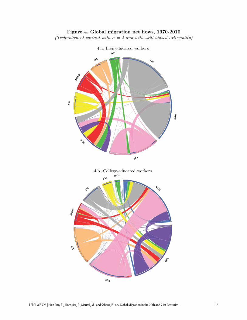
Figure 4. Global migration net flows, 1970-2010(Technological variant with σ = 2 and with skill biased externality)

4.a. Less educated workers

LAC

NAM

SEA

EUR

SSA

MENA

CIS

OTH

4.b. College-educated workers

NAM

EUR

SEA

CIS

MENA

LAC

SSA

OTH


Major corridors by skill group. – We now characterize the clusters of origins and destina-tions that caused the greatest variations in global migration between 1970 and 2010. Usingthe same matrix of migration net flows as above (denoted byM and including the J ×J netflows between 1970 and 2010, ∆Mij,s), our objective is to identify a sub-matrix with a fixeddimension o×d that maximizes the total migration net flows (i.e., that captures the greatestfraction of the worldwide variations in migration stocks). The Max-Sum Submatrix problemcan be defined as:

Definition 2 Given the squared matrix M ∈ RJ×J of net migration flows between J originand J destination countries, and given two numbers o and d (the dimensions of the subma-trix), the Max-Sum submatrix is a submatrix (O∗, D∗) of maximal sum , with O∗ ⊆ J andD∗ ⊆ J , such that:

(O∗, D∗) =O⊆J ,D⊆J∑

i∈O,j∈DMij . (8)

|O| = o and |D| = d (9)

where J = {1, . . . , J}.

This problem is a variant of the one introduced in Dupont et al. (2017) or Le Vanet al. (2014). The difference is that we fix the dimension of the submatrix. It also hassome similarity with the bi-clustering class of problems for which a comprehensive reviewis provided in Madeira and Oliveira (2004). To solve the Max-Sum Submatrix problem, weformulate it as a Mixed Integer Linear Program (MILP):15

maximize∑

i∈O,j∈DMij ×Xij , (10)

s.t. Xij ≤ Ri, ∀i ∈ O,∀j ∈ D , (11)

Xij ≤ Cj, ∀i ∈ O,∀j ∈ D , (12)

Xij ≥ Ri + Cj − 1, ∀i ∈ O,∀j ∈ D , (13)∑i∈O Ri = o , (14)∑j∈D Cj = d , (15)

Xij ∈ {0, 1}, ∀i ∈ O,∀j ∈ D , (16)

Ci ∈ {0, 1}, ∀i ∈ O , (17)

Rj ∈ {0, 1}, ∀j ∈ D . (18)

A binary decision variable is associated to each origin-row Ri, and to each destination-column Cj, and to each matrix entry Xij. The objective function is computed as the sum ofmatrix entries whose decision variable is set to one. Eqs. (11) to (13) enforce that variableXi,j = 1 if and only both the row i and column j are selected (Ri = 1 and Cj = 1). Thisformulation is the standard linearization of the constraint Xij = Ri · Cj. Constraints (14)and (15) enforce the o× d dimension of the submatrix to identify.

Applying the Max-Sum problem to the net flows of low-skilled migrants, we can identifythe 25 origins and the 25 destinations of the Max-Sum submatrix. These 625 entries of thesubmatrix account for 64% of the worldwide net flows of low-skilled migrants between 1970and 2010.

15See Nemhauser and Wolsey (1988) for an introduction to MILP.


• The main destinations (in alphabetical order) are: Australia, Austria, Belarus, Belgium,Canada, Dominican Republic, France, Germany, Greece, Hong Kong, India, Israel,Italy, Kazakhstan, Malaysia, Nepal, the Netherlands, Oman, Russia, Saudi Arabia,Spain, Thailand, the United Kingdom, the United States, and Venezuela.

• The main origins (in alphabetical order) are: Albania, Algeria, Bangladesh, Colom-bia, the Dominican Republic, Ecuador, Guatemala, Haiti, India, Indonesia, Jamaica,Kazakhstan, Mexico, Morocco, Myanmar, Pakistan, the Philippines, Poland, Romania,Russia, Slovenia, Turkey, Ukraine, Uzbekistan, and Vietnam.

As far as high-skilled migrants are concerned, the set of main destinations mostly includeshigh-income countries. The 625 entries of the submatrix account for 55% of the worldwidenet flow of college-educated migrants between 1970 and 2010.

• The 25 main destinations (in alphabetical order) are: Australia, Austria, Belarus,Canada, France, Germany, India, Ireland, Israel, Italy, Japan, Kazakhstan, the Nether-lands, New Zealand, Oman, Russia, Saudi Arabia, Spain, Sweden, Switzerland, Thai-land, Ukraine, the United Arab Emirates, the United Kingdom, and the United States.

• The 25 main origins (in alphabetical order) are: Algeria, Bangladesh, Canada, China,Colombia, Egypt, France, Germany, India, Iran, Japan, Kazakhstan, Mexico, Morocco,Pakistan, the Philippines, Poland, Romania, Russia, South Korea, Ukraine, the UnitedKingdom, the United States, Uzbekistan, and Vietnam.

Aggregate TFP externalities. – Finally, the backcasting exercise allows calibration of theTFP level (Aj,t) for each country, for each decadal year, and for each pair (σ, κ). We can usethese calibrated TFP levels to estimate the size of the aggregate TFP externality, ε. In linewith Eq. (5), we regress the log of TFP on the log of the skill ratio, controlling for time fixedeffects (capturing λt) and for country fixed effects (capturing Aj). Identifying the size of theTFP externality is important for conducting the forecasting exercise. Results are reportedin Table 2. We identify a significant and positive effect when the skill biased externalityoperates fully; the greatest level (0.207) is obtained in column 1, when σ = 2 and κ = 0.214.Lower levels of ε are obtained when σ = 3 (0.105) and/or when κ increases.

Table 2. Estimating ε using panel regressions, 1970-2010(Dependent = logAj,t)

(1) (2) (3) (4) (5) (6)

σ = 2 σ = 2 σ = 2 σ = 3 σ = 3 σ = 3κ = 0.000 κ = 0.107 κ = 0.214 κ = 0.000 κ = 0.024 κ = 0.048

log (Lj,h,t/Lj,l,t) 0.041 0.132∗∗∗ 0.207∗∗∗ 0.063 0.085∗∗ 0.105∗∗

(0.043) (0.043) (0.044) (0.043) (0.043) (0.043)

Constant 8.055∗∗∗ 8.493∗∗∗ 8.865∗∗∗ 8.392∗∗∗ 8.490∗∗∗ 8.568∗∗∗

(0.260) (0.254) (0.252) (0.257) (0.256) (0.255)

Time FE yes yes yes yes yes yes

Country FE yes yes yes yes yes yes

R-squared 0.912 0.915 0.918 0.899 0.900 0.901

Nb. obs. 900 900 900 900 900 900


4 Forecasting

We now use the parameterized model to produce projections of migration stocks and incomedisparities for the 21st century. Availability of population projection until the end of thecentury allows us to systematically predict migration for that entire period. Nonethelesssince the accuracy of prediction decreases with time, we will mainly focus on interpretingresults of the medium-term forecasts (up to 2050). We first define the two socio-demographicscenarios that feed our model; one has optimistic predictions for human capital while theother is more pessimistic. We then describe the global trends in international migration andincome inequality involved in these two scenarios, with a special focus on migration flowsto OECD countries. We finally discuss the policy options than can be used to curb futuremigration pressures.

Socio-demographic scenarios. – Our socio-demographic scenarios are drawn from Lutzet al. (2014), who produce projections by age, sex and education levels for all countries ofthe world. As human capital changes affect the distribution of productive capacities, incomeinequality and the propensity to migrate of people, we distinguish between an optimisticand a pessimistic scenario (labeled as SSP2 and SSP3, respectively). The authors defineSSP2 as a Continuation/Medium Population scenario, which is described as follows: ”this isthe middle-of-the-road scenario in which trends typical of recent decades continue, with someprogress towards achieving development goals, reductions in resource and energy intensity,and slowly decreasing fossil fuel dependency. Development of low income countries is un-even, with some countries making good progress, while others make less.” As for SSP3, it isdefined as the Fragmentation/Stalled Social Development scenario, which is described as fol-lowsg: ”this scenario portrays a world separated into regions characterized by extreme poverty,pockets of moderate wealth, and many countries struggling to maintain living standards forrapidly growing populations. The emphasis is on security at the expense of internationaldevelopment.”

The SSP2 and SSP3 scenarios involve international migration hypotheses, which are notin line with our migration technology. To neutralize these migration hypotheses, we use thescenario-specific projections of net immigration flows (Ii,s,t) from Lutz et al. (2014), and weproxy the evolution of the native population (Ni,s,t) by education level from 2010 to 2100. Inpractice, the dynamics of the resident population is governed by:

∆Li,s,t = ∆Mii,s,t + Ii,s,t,

where ∆Li,s,t = Li,s,t−Li,s,t−1 is the change in the level of the resident, working-age population(available at each period), Ii,s,t stands for the net inflow of working-age immigrants (i.e.immigrants minus emigrants) to country i and for the education level s, and ∆Mii,s,t =Mii,s,t −Mii,s,t−1 stands for the change in the number of native non-migrants.

Using official projections for ∆Li,s,t and Ii,s,t, we extract ∆Mii,s,t from this equation.Remember that the DIOC-E database of the OECD allows us to estimate the size of thenative population, Ni,s,2010, and of the native non-migrant population, Mii,s,2010, for the year2010. We can thus recursively compute ∆Mii,s,t/Mii,s,t−1 and the level of Mii,s,t for all yearsafter 2010. Assuming that ∆Ni,s,t/Ni,s,t−1 = ∆Mii,s,t/Mii,s,t−1 (i.e. the growth rate of thenative population equals the growth rate of the native non-migrant population), we thenproxy the evolution of the native population for all years after 2010.


Figure 5 describes the two socio-demographic scenarios. Figure 5.a compares the trajec-tories of the worldwide population aged 25 to 64 over the 21st century. In the SSP2 scenario,the working-age population increases by 31%, from 3.28 billion in 2010 to 4.29 billion in 2100.Figure 5.c illustrates the evolution of the regional shares in the world population. The break-down by region and the choice of colors are similar to Figure 4, albeit slightly less detailed forexpositional convenience. The demographic share of OECD member states decreases from19.2 to 14.8% (-4.4 percentage points), and that of Asia decreases from 54.6 to 40.0% (-14.6percentage points). By contrast, the share of sub-Saharan Africa drastically increases from8.4 to 28.5% (+20.1 percentage points). The shares of MENA countries (+2.3 percentagepoints), of Latin American countries (-1.1 percentage points), and of the rest of the world(-2.2 percentage points) exhibit smaller variations. In the SSP3 scenario, the working-agepopulation increases by 90% and reaches 6.26 billion in 2100. Figure 5.d shows that thedemographic share of OECD member states decreases from 19.2 to 8.8% (-10.4 percentagepoints), and that of Asia decreases from 54.6 to 45.8% (-8.8 percentage points). The share ofsub-Saharan Africa increases from 8.4 to 27.0% (+18.6 percentage points). Demographicallyspeaking, the difference between these two scenarios is mainly perceptible after the year 2050,and concerns the shares of OECD and Asian countries.

Figure 5.b compares the trajectories of the worldwide proportion of college graduates inthe working-age population. In the SSP2 scenario, this proportion increases by 31.6 percent-age points, from 14.7% in 2010 to 46.3% in 2100. Between 1970 and 2010, the worldwideshare of college graduates increased by 2.3 percentage point per year under the impetus ofhigh-income countries; it increased by 1.9 percentage points per year in developing countries,and by 2.1 percentage points per year in sub-Saharan Africa. For the years 2010 to 2100,SSP2 predicts a rise of 3.5 percentage point per year for the world and for the set of develop-ing countries, against +0.5 percentage points in Africa. By contrast, SSP3 predicts a slightdecrease in human capital for the world and for the set of developing countries, and +1.2 peryear in Africa. Figure 5.e illustrates the evolution of the regional shares in the world stock ofhuman capital. In 2100, 40.1 % of college graduates are living in the OECD member states;this share decreases by 17.9 percentage points between 2010 and 2100. The share of Asiaincreases from 36.9 to 39.9% (+3.0 percentage points), and the share of sub-Saharan Africadrastically increases from 3.1 to 18.4% (+15.3 percentage points); the latter change is dueto the rising demographic share of Africa. In the SSP3 scenario, the proportion of collegegraduates decreases slightly, from 14.7% in 2010 to 13.0% in 2100. Figure 5.f shows that thehuman capital share of OECD member states decreases from 40.2 to 20.4% (-19.8 percent-age points). The share of Asia increases from 36.9 to 42.2% (+5.3 percentage points). Theshare of sub-Saharan Africa increases from 3.1 to 13.5% (+10.4 percentage points). As far aseducation is concerned, the major difference between these two scenarios is the evolution ofhuman capital in low-income countries in general, and in sub-Saharan Africa in particular.


Figure 5. Socio-demographic scenarios, 2010-21005.a. World population (billions) 5.b. Share of college graduates (%)

1

2

3

4

5

6

1970 1980 1990 2000 2010 2020 2030 2040 2050 2060 2070 2080 2090 2100

SSP2 SSP3

0

10

20

30

40

50

1970 1980 1990 2000 2010 2020 2030 2040 2050 2060 2070 2080 2090 2100

SSP2 SSP3

5.c. Population shares by region in SSP2 5.d. Population shares by region in SSP3

0

10

20

30

40

50

60

70

80

90

100

1970 1980 1990 2000 2010 2020 2030 2040 2050 2060 2070 2080 2090 2100

OECD SSA MENA LAC Asia Others

0

10

20

30

40

50

60

70

80

90

100

1970 1980 1990 2000 2010 2020 2030 2040 2050 2060 2070 2080 2090 2100


5.e. Shares of college graduates in SSP2 5.f. Shares of college graduates in SSP3

0

10

20

30

40

50

60

70

80

90

100

1970 1980 1990 2000 2010 2020 2030 2040 2050 2060 2070 2080 2090 2100


0

10

20

30

40

50

60

70

80

90

100

1970 1980 1990 2000 2010 2020 2030 2040 2050 2060 2070 2080 2090 2100


Global implications. – We turn now to the implications of our two socio-demographicscenarios for income growth, global inequality and migration pressures. It is importantto acknowledge the reverse impacts of migration on population growth in sending countries.They are however not accounted for in this prospective paper, which takes socio-demographicscenarios as given in order to analyze their effects on income and migration. In addition tothat, the longer the distance from 2010, the more uncertain are our projections. We caninfer the predictability of our model from the reported coefficients of determination in Table


1 and Figure 3, which decrease with time departing from 2010 back to the past. Moreover,our forecasts do not account for future conflict, global warming, etc.. Compared to thesefactors that also affect migration, demography has higher level of predictability and can beseen as the driver of natural migration trend. Lastly, in all simulations we consider constantnet migration costs Vij,s,2010, which perform very well in backcasting past migration.

Figure 6. Global income and migration forecasts, 2010-2100

6.a. World GDP per worker 6.b. Theil index

0

20000

40000

60000

80000

1970 1980 1990 2000 2010 2020 2030 2040 2050 2060 2070 2080 2090 2100

SSP2/s2/0% SSP2/s2/50% SSP2/s2/100%SSP2/s3/0% SSP3/s2/0%

.2

.3

.4

.5

.6

.7

.8

1970 1980 1990 2000 2010 2020 2030 2040 2050 2060 2070 2080 2090 2100


6.c. World proportion of migrants 6.d. Share of college-educated migrants

3.5

4

4.5

5

5.5

6

1970 1980 1990 2000 2010 2020 2030 2040 2050 2060 2070 2080 2090 2100


0

20

40

60

80

1970 1980 1990 2000 2010 2020 2030 2040 2050 2060 2070 2080 2090 2100


6.e. Emigration rates from developing countries 6.f. Immigration rate to OECD countries

3

4

5

6

1970 1980 1990 2000 2010 2020 2030 2040 2050 2060 2070 2080 2090 2100


5

10

15

20

25

30

1970 1980 1990 2000 2010 2020 2030 2040 2050 2060 2070 2080 2090 2100



The global income and migration forecasts are depicted on Figure 6, which combines thedata for the period 1970-2010, and the model forecasts for the subsequent years. We dis-tinguish between five scenarios. In the first three ones, we consider that socio-demographicvariables are governed by SSP2, and we combine it with the three technological variantsdefined in Columns (1), (2) and (3) of Table 2 (i.e., σ = 2 and technological externalitiesequal to 0, 50 or 100% of the correlation between productivity levels and the skill ratio).While keeping SSP2, the fourth scenario assumes σ = 3 and zero technological externalities(as in Column (4) of Table 2). Finally, the fifth scenario combines SSP3 with σ = 2 andfull technological externalities (as in Column (6) of Table 2). In all scenarios with or with-out technological externalities, we assume an exogenous increase in TFP of 1.5% per year.It is worth noticing that under SSP3, worldwide changes in human capital are negligible;eliminating technological externalities hardly modifies the results.

Let us first focus on income projections. Figure 6.a shows the evolution of the worldwidelevel of GDP per worker. Under SSP3, the average GDP level in the year 2100 is 2.4 timesgreater than the level observed in 2010 (i.e., a growth rate of 1.0% per year). Under SSP2and due to the rise in the level of schooling, the GDP level in 2100 is 3.5 times greater thanthe level observed in 2010 (i.e., a growth rate of 1.4% per year). Productivity growth isboosted when technological externalities are factored in. Assuming externalities are equal to50 or 100% of the correlation, the annual growth rate reaches 1.7 and 1.9%, respectively.Finally, assuming a higher level for σ generates very similar income projections. Figure 6.bdescribes the evolution of the Theil index between 1970 and 2100. We combine our backcastsand forecasts, and account for between-country inequality and within-country inequality(between the college-educated and less educated representative workers, only). Globally, weshow that the Theil index decreases from 1970 to 2010, a phenomenon that can be due toconvergence in the productivity scale factors. Our projections do not account for convergenceforces that are not driven by human capital. Under SSP2, the model predicts that the Theilindex is constant over time, or is increasing slightly when externalities are included. UnderSSP3, we predict a larger increase in the Theil index.

Figures 6.c and 6.d depict the evolution of the worldwide proportion of internationalmigrants and of the skill structure of migration. Under SSP3, the proportion of migrants(ranging from 3.6 and 3.9%) and the share of college-educated (around 30%) are fairly stable.By contrast, under SSP2, progress in education makes people more mobile. Under constantmigration policies, the proportion of migrants increases from 3.6% in 2010 to 4.5% in 2050and to 6.0% in 2100, and the share of college graduates increases from 29% in 2010 to34% in 2050 and to 70% in 2100. It is worth noticing that in Figure 6.c the importantgap between the proportions of migrants in SSP2 and SSP3 does not result from a bigdifference in terms of migrant volume. In 2010, the working-age population is estimated at3.28 billion, it will increase by 2100 to 4.29 billion according to SSP2, and more drasticallyto 6.26 billion following SSP3. While using SSP2 we predict a net increase in total migrantsbetween 2010 and 2100 of about 111 million people, this number is a little bit smaller usingSSP3 which is about 82 million. As regards the proportion of the high skill population, itshould be recalled that our backcasts reveal that past changes in educational attainmentwere small in developing countries; they hardly affected the trajectory of global migration(see Figure 2.b). SPP2 predicts large educational changes in the coming decades, with strongimplications for global migration. Another remarkable result is that the global trends in


international migration are virtually unaffected by the technological environment; they aretotally governed by socio-demographic changes.

We now focus on emigration and immigration rates, separately. Figure 6.e depicts theevolution of emigration rates, defined as the ratio of emigrants to natives originating fromdeveloping countries. The average emigration rate equals 3.1% in 2010. Under SSP2, it ispredicted to reach 4.1% in 2050 and to be twice as large in the year 2100; under SSP3, itreaches 3.6% only by the end of the century. As explained above, the emigration rate isgoverned by the change in the average level of education in the developing world. UnderSSP2 progress in education makes people more mobile (remember college graduates migratemore than the less educated). Under SSP3 emigration rates remain fairly stable over timegiven the slower progress in education. Similar patterns exhibit in both Figures 6c and 6esuggesting that the world proportion of migrants is shaped by emigration rates from devel-oping countries. Finally, Figure 6.f depicts the evolution of the average immigration rateof OECD member states, defined as the proportion of foreign-born in the total population.This proportion equals 12% in the year 2010 and it is expected to increase drastically overthe 21st century. Nevertheless, a remarkable result is that the magnitude of the change ishighly insensitive to socio-demographic and technological scenarios. Under SSP3, emigrationrates from developing countries vary little, but population growth is large. Under the SSP2scenario, the rise in emigration rates is larger, but it is partly offset by the fall in the popula-tion growth rates of developing countries. By the year 2100, the share of immigrants reaches27.8% under SSP2, and 24.6% under SSP3.

In Figure 7, we represent the net flows of low-skilled and high-skilled migrants over the 21stcentury. Origin and destination regions are represented by circular ideograms (Kzrywinskiet al., 2009), and we use the same regions and colors as in Figure 4. Net flows are coloredaccording to their origin, and their width is proportional to their size. The direction of theflow is captured by the colors of the outside (i.e., country of origin) and inside (i.e., countryof destination) borders of the circle.

Figures 7.a and 7.b show the net flows of low-skilled migrants under the SSP2 and SPP3socio-demographic scenario, respectively. Under SPP2, the total net flows amount to 32 mil-lion. The top-5 regional corridors are intra-African migration (24.3% of the total), migrationfrom South and East Asia to the MENA (13.8%), migration from sub-Saharan Africa to Eu-rope (13.7%), intra-MENA migration (8.7%), and migration from Latin America to Westernoffshoots (8.4%). Outflows from sub-Saharan Africa and South and East Asia to Europe arelarge. Under SPP3, the total net flows amount to 60 million and are greater for all regionalcorridors. Compared to Figure 7.a, Figure 7.b of scenario SSP3 with slower growth andgreater fertility rates shows large outflows from Latin America to North America and withinAfrican regions. The top-5 regional corridors are Latin America to Western offshoots (16.4%of the total), intra-African migration (15.3%), intra-MENA migration (11%), migration fromSouth and East Asia to Western offshoots (21.1%), and migration within South and EastAsian countries (9.3%).


Figure 7. Global migration net flows, 2010-2100(Technological variant with σ = 2 and with technological externalities)

7.a. Less educated workers (SSP2)

SSA

SEA

MENA

EUR

NAM

LAC

OTHCIS

7.b. Less educated workers (SSP3)

SSA

MENA

SEA

LAC

NAM

EUR

OTH

CIS


Figure 7. Global migration net flows, 2010-2100 (cont’d)(Technological variant with σ = 2 and with technological externalities)

7.c. College-educated workers (SSP2)

NAM

SEA

EUR

MENA

SSA

LAC

CIS

OTH

7.d. College-educated workers (SSP3)

NAM

SEA

MENA

EUR

SSA

LAC

CISOTH


Figures 7.c and 7.d show the net flows of college-educated migrants under the SSP2 andSPP3 socio-demographic scenario, respectively. Under SPP2, the total net flows amount to79 million. The top-5 regional corridors are migration from South and East Asia to Westernoffshoots (21.1%), migration from sub-Saharan Africa to Europe (10.2%), migration fromLatin America to Western offshoots (10.1%), migration from sub-Saharan Africa to Westernoffshoots (7.8%), and migration from South and East Asia to the MENA (6.6%). Inflowsto Western offshoots and Europe are large. Under SPP3, the total net flow amounts to 22million only, but the structure of worldwide migration is similar than under SSP2. The top-5regional corridors are migration from South and East Asia to Western offshoots (24.2%),migration from Latin America to Western offshoots (11.5%), migration from sub-SaharanAfrica to Europe (10.4%), migration from sub-Saharan Africa to Western offshoots (8.2%),and intra-MENA migration (8.0%).

Implications for HI countries. – Table 3 provides projections of immigration rates for themain high-income, destination countries and for constant immigration policies (remember thishypothesis performed well when producing backcasting results). Results obtained under theSSP2 socio-demographic scenario are presented in the top panel; results obtained under SSP3are presented in the bottom panel. In both cases, we consider the variant with σ = 2 and fulltechnological externalities, the scenario that is the most compatible with future educationalchanges.16 Under SSP2 and over the 21st century, the proportion of immigrants increases by21.2% in the EU15 and by 14.3% in the United States. The greatest variations are obtainedfor the United Kingdom (+35.9%) and for Canada (+35.6%). Under SSP3, the averagepopulation growth rates are larger in developing countries, with the exception of Asia. Theproportion of immigrants increases by 24.3% in the EU15 and by 22.4% in the United States.The greatest variations are obtained for Spain (+27%), the United Kingdom (+26.2%) andfor Canada (+29.8%). Projections for the coming 50 years are rather insensitive to thesocio-demographic scenario.

In line with Hanson and McIntosh (2016) or with Docquier and Machado (2007), futuremigration pressures mainly affect European countries, and are mostly due to rising migrationflows from developing countries. To illustrate this, we use the same Max-Sum Submatrixalgorithm as in the previous section, and apply it to the matrix of total migration net flowsfrom developing countries to the 27 members of the European Union between 2010 and 2060;projections for subsequent years are more uncertain and scenario-sensitive. For each socio-demographic scenario, we identify the sub-matrix with a fixed dimension of 25 × 10 thatmaximizes the total migration net flows.

Under the SSP2 scenario, we obtain the following results (in alphabetical order):

• Main destination countries: Belgium, France, Germany, Ireland, Italy, Netherlands,Portugal, Spain, Sweden, and the United Kingdom.

• Main countries of origin: Afghanistan, Algeria, Angola, Bangladesh, Cameroon, Dem.Rep. of Congo, Cote d’Ivoire, Ghana, India, Iran, Iraq, Kenya, Madagascar, Mali,Morocco, Mozambique, Nigeria, Pakistan, Philippines, Senegal, Somalia, Tanzania,Turkey, Uganda, and Zimbabwe.

16Very similar results are obtained when technological externalities are zero, as shown in Table A1 in theAppendix.


Table 3. Proportion of working-age immigrants by main destination(Scenario with σ = 2 and full technological externality)

2010 2020 2030 2040 2050 2060 2070 2080 2090 2100 ∆SSP2, σ = 2, full technological externalities

EU15 14.5 16.8 19.3 22.2 24.7 26.8 29.1 31.3 33.5 36.5 +21.2

France 14.7 18.0 21.0 24.0 26.2 28.2 30.3 32.4 34.4 36.5 +21.8

Germany 15.9 17.3 19.3 21.3 22.0 22.8 23.7 24.0 24.3 24.9 +9.0

Italy 10.5 11.8 13.1 14.8 15.9 16.3 16.9 17.6 18.1 18.7 +8.2

Spain 14.9 16.8 19.2 22.0 25.2 26.6 27.6 28.9 29.5 29.9 +15.0

United Kingdom 16.5 19.9 24.2 28.8 32.8 37.2 41.1 45.1 48.9 52.3 +35.9

Switzerland 31.4 33.2 35.7 38.8 40.7 42.9 45.0 46.9 48.9 51.0 +19.6

United States 17.7 20.4 23.3 25.2 26.7 28.0 29.1 30.1 30.9 31.9 +14.3

Canada 24.5 29.4 35.3 40.1 44.3 48.4 51.7 54.5 57.3 60.0 +35.6

Australia 28.7 31.2 33.8 36.3 38.4 40.7 42.5 44.3 46.3 48.2 +19.4

OECD 11.9 13.7 15.5 17.4 19.2 20.8 22.5 24.2 25.8 27.5 +15.6

SSP3, σ = 2, full technological externalities

EU15 14.5 16.4 18.4 20.7 22.8 25.3 28.2 31.9 35.4 38.9 +24.3

France 14.7 17.4 19.4 21.2 22.7 24.6 27.1 30.3 33.3 36.3 +22.2

Germany 15.9 17.3 19.3 21.5 23.2 25.6 28.9 32.3 36.0 40.0 +24.1

Italy 10.5 11.8 13.2 15.2 17.3 19.3 21.8 25.4 28.6 32.1 +21.6

Spain 14.9 16.6 18.7 21.4 25.2 28.1 31.0 35.4 38.8 41.9 +27.0

United Kingdom 16.5 18.6 21.3 23.4 25.5 28.6 31.7 35.8 39.8 43.6 +26.2

Switzerland 31.4 32.5 34.1 36.1 37.3 39.3 41.5 44.1 46.9 49.7 +18.4

United States 17.7 19.8 22.2 23.5 25.3 27.6 30.2 33.6 36.8 40.1 +22.4

Canada 24.5 27.4 31.2 33.5 35.7 39.1 42.3 46.3 50.3 54.2 +29.8

Australia 28.7 29.9 31.4 32.4 33.5 35.5 37.6 40.5 43.8 47.0 +18.2

OECD 11.9 13.3 14.6 15.7 16.9 18.3 19.8 21.6 23.2 24.6 +12.7

And under the SSP3 scenario, we have (by alphabetical order):

• Main destination countries: Austria, Belgium, France, Germany, Italy, Netherlands,Portugal, Spain, Sweden, and the United Kingdom.

• Main countries of origin: Afghanistan, Algeria, Angola, Bangladesh, Bolivia, Colombia,Dem. Rep. of Congo, Cote d’Ivoire, Ecuador, Ghana, India, Iraq, Kazakhstan, Kenya,Madagascar, Mali, Morocco, Nigeria, Pakistan, Peru, Philippines, Senegal, Somalia,Turkey, and Uganda.

Under SSP2, migration flows from sub-Saharan Africa and from the MENA play a keyrole, as well as the flows from a few Asian countries with large populations. As the majorityof African migrants go to Europe, the EU15 experience greater migration pressures. UnderSSP3, this change is mostly due to immigration from Africa, although the magnitude of thisphenomenon is smaller than under SSP2. However, migration pressures from Asia, from


MENA, and from some Latin American countries are stronger. Clearly, there is a large inter-section of 9 destination countries (see countries in italics above) that are all member statesof the EU15, and for which future migration pressures are expected to be strong, whateverthe socio-demographic scenario for the coming half century. And there is large intersection of20 developing countries (in italics above) that are responsible for such migration pressures,including sub-Saharan African countries, the MENA countries, and a few Asian countries.

The case for Migration Compacts. – In line with the Sustainable Development Goals andthe New York Declaration for Refugees and Migrants (United Nations, 2016), the EuropeanCommission has outlined a general line of action to cope with the global challenge of futuremigration (see the European Agenda on Migration and the new Partnership Framework onMigration). Migration Compacts have been designed for Jordan, Lebanon, Nigeria, Niger,Mali, Senegal, Morocco, Tunisia, Libya and Ethiopia as of 2017; they can also be implementedin other partner countries. They include a set of measures to be implemented in the homecountry, targeting the reinforcement of border controls, the readmission of migrants whohave been denied entry, or a higher level of economic development. Readmission and bordercontrol strategies are difficult to implement in fragile states. Under the European MigrationCompacts, an investment plan has also been proposed to stimulate employment opportuni-ties and income in Africa, in the hope of reducing migration pressures. The effectivenessof these Migration Compacts depends on the resources allocated to their implementation(in comparison to the development targets to be reached), and on the effectiveness of themeasures undertaken.

To illustrate the difficulty curbing future migration pressure, we consider the intersectionof 20 developing countries emerging from our Max-Sum Submatrix problem (referred to asCompact 1 ),17 or the combined region of sub-Saharan African and the MENA countries(referred to as Compact 2 ). We consider these sets of countries as potential partners of aMigration Compact, and we quantify the homothetic change in TFP (above normal trend)and derive the consequent GDP annual growth rates required to keep their total emigrationstocks to Europe at their levels of 2010. Our simulations account for all general equilibriumeffects.

Table 4 provides the results of these policy experiments, taking the population size andstructure as given. Our discussion mainly focuses on net migration flows in the next twodecades, the period for which socio-demographic variations between SPP2 and SPP3 aresmaller and less likely to be affected by the TFP changes. In other words, this considerationpartially mitigates the issue that fertility and human capital are endogenously affected byincome, which our model does not account for. Indeed, if TFP and GDP start increasing from2010 onwards, population growth rates and the skill composition of the labor force will begradually impacted. Results obtained for 2030 and after (essentially beyond one generation)are likely to overestimate the requested changes and should be treated with more caution.

Under the SSP2 socio-demographic scenario, keeping the stock of the 20 main origincountries (Compact 1 ) at its level of 2010 requires TFP to increase by 58% in 2020 and by128% in 2030, compared to the baseline. Under the SSP3 scenario, the required TFP changes

17These include Afghanistan, Algeria, Angola, Bangladesh, Dem. Rep. of Congo, Cote d’Ivoire, Ghana,India, Iraq, Kenya, Madagascar, Mali, Morocco, Nigeria, Pakistan, Philippines, Senegal, Somalia, Turkey,and Uganda.


amount to 49% in 2020 and by 99% in 2030. Overall, this means multiplying GDP per capitaby 2 above the normal trend over the next two decades. Equivalently, this requires a TFPgrowth rate of 5% per year under SPP2 (instead of 1.5% a year in the baseline), and a TFPgrowth rate of 4.2% a year under SPP3. In terms of GDP growth, the required levels areon average twice as high as the baseline levels; in all variants, the requested annual GDPgrowth rate is close to 10%. Implementing Migration Compacts with all sub-Saharan Africanand MENA countries (Compact 2 ) requires similar changes in TFP and gives rise to similareffects.18

Table 4. Development policies to limit migration pressures

2010 2020 2030 2040 2050 2060 2100

I. Socio-demographic scenario: SSP2

Baseline immigration rate to EU15 14.6 16.8 19.3 22.2 24.7 26.8 35.8

Compacts 1 I.a. 20 main origin countries

TFP change: Aj,t/ABasej,t 1.00 1.58 2.28 3.19 4.18 5.24 9.73

New immigration rate EU15 14.6 15.6 16.9 18.5 19.5 20.4 24.9

Mean annual GDP growth over decade (Base) 5.17 5.00 4.82 4.58 4.33 3.48

Mean annual GDP growth over decade 10.28 9.59 9.11 8.54 7.99 6.25

Compacts 2 I.b. All sub-Saharan Africa and MENA





II. Socio-demographic scenario: SSP3

Baseline immigration rate to EU15 14.6 16.4 18.4 20.7 22.8 25.3 38.9

Compacts 1 II.a. 20 main origin countries





Compacts 2 II.b. All sub-Saharan Africa and MENA




Mean annual GDP growth over decade 8.95 8 7.38 6.84 6.42 5.22

Takeoffs of this nature have rarely been observed in the course of history.19 They basically

18We have also conducted another set of simulations (Compact 3 ) keeping constant the total emigrationstocks of sub-Saharan African countries only. The resulting required TFP growth rates are much higherthan the ones in Compact 2 where growth is fostered in both the MENA and SSA regions. This shows thecapacity of the MENA countries to absorb migrants from SSA. Thus smaller but simultaneous investment inboth regions is recommended to keep immigration rates in Europe at constant levels.

19This was even the case during the Industrial Revolution. Between 1820 and 1900, GDP per capita rose2.5 times in Western Europe, and 3.3 fold in the United States (Maddison, 2007). In other words, growthrates were 1.2 and 1.5% a year, respectively.


require all SSA and MENA countries to enter the ”modern growth club” during the 21stcentury. Based on facts from the 19th and 20th centuries, Benetrix et al. (2015) estimatethat joining the club requires an annual GDP growth rate above 5% over a period of tenyears; Jones and Romer (2010) argue that higher threshold growth rates are needed in thecurrent period. Still, ”explosive-growth” episodes were indeed recently observed in emergingcountries. Taiwan multiplied its income per capita by 5 between 1980 and 2000, and SouthKorea multiplied it by 7.5 over the same period; China has increased its income level tenfoldsince 1990 with an average GDP growth rate of 8% per year. Similar takeoffs have not beenobserved in sub-Saharan Africa. However, Rwanda, which is usually seen as one of the fastestgrowing economies in Africa, has increased its income per capita threefold since the genocide.

Sustaining TFP growth rates of 4 to 5% or real GDP growth rates of 8 to 10% peryear on the spatial scale of a continent and over several decades is unprecedented. So far,development policies have not triggered such resounding and generalized economic booms.Hence, dramatic changes in the effectiveness of aid are needed if policymakers want to usedevelopment tools to reduce migration pressures (Berthelemy et al. 2009; Berthelemy andMaurel 2010; Gary and Maurel 2015). In addition, generating these booms in SSA and MENAwould only attenuate migration pressures to Europe, but would not eliminate them sincemigration pressures from other countries and regions would still be observed. Table 4 showsthat the EU15 immigration rate in 2060 would be around 20% in all scenarios, comparedto 14.6% in 2010. Reinforcing immigration restrictions is another complementary policyavenue. However, it is a priori unclear whether changes in laws and policies can significantlyaffect the size of immigration flows. Past restrictions on migration have not prevented third-country nationals from moving in past decades (it may be recalled that our backcasts withconstant Vij,s,t fit well past migration flows), and have caused displacements and increasingflows of irregular migrants. Over the 21st century, increasing migration seems to be aninevitable phenomenon, which raises important challenges in terms of policy coherence formost industrialized countries.

5 Conclusion

The number of asylum applications lodged in 2015 in EU Member States exceeded 1.3 million,putting migration policy in the forefront of the global policy debate. While the proximatecause of the current crisis is the conflict and political unrest in the Middle East and Africa, therecent trends and forecasts for the world economy strongly suggest that there may be furtherepisodes of large-scale migration in the near future, in Europe and in other OECD countries.Specifically, the underlying root causes of increased migration (demographic imbalances,economic inequality, increased globalization, political instability, climatic changes) are allprojected to exert a stronger influence in the coming decades.

Relying on socio-demographic and technological scenarios, this paper produces integratedbackcasts and forecasts of income and bilateral migration stocks for all pairs of countries.Our model fits very well the trends in international migration of the last 40 years, anddemonstrates that historical trends were mostly governed by demographic changes. Turningto the migration prospects for the 21st century, we also find that world migration prospectsare mainly governed by socio-demographic changes; they are virtually insensitive to the


technological environment. We predict a highly robust increase in immigration pressures ingeneral, and in European immigration in particular. These migration pressures are mostlyexplained by the demographic changes in sub-Saharan Africa and in the MENA countries.Curbing them with development policies requires triggering unprecedented economic boomsin many developing countries. More than ever, improving the management of migrationflows and the coherence between development and migration policies will represent majorchallenges for European countries in the 21st century.

References

[1] Acemoglu, D. (2002). Technical Change, Inequality, and the Labor Market. Journal ofEconomic Literature 40(1): 7-72.

[2] Acemoglu, D. & J. Angrist (2001). How large are human-capital externalities? Evi-dence from compulsory schooling laws. In: B.S. Bernanke & K. Rogo (eds.), NBERMacroeconomics Annual 2000, volume 15, Cambridge, MA: MIT Press.

[3] Autor, D.H. & F. Levy & R.J. Murnane (2003). The Skill Content of Recent Tech-nological Change: An Empirical Exploration. Quarterly Journal of Economics 118(4):1279-1333.

[4] Beine, M. & P. Bourgeon.& J.C. Bricongne (2013). Aggregate Fluctuations and Inter-national Migration. CESifo Working Paper Series 4379, CESifo Group Munich.

[5] Beine, M. & C. Parsons (2015). Climatic Factors as Determinants of International Mi-gration. Scandinavian Journal of Economics 117(2): 723-767.

[6] Benetrix, A. & K. O’Rourke & J. Williamson (2015). The spread of manufacturing tothe poor periphery 1870-2007. Open Economies Review 26(1): 1-37.

[7] Benhabib, J. & M.M. Spiegel (1994). The Role of Human Capital in Economic Develop-ment: Evidence from Aggregate Cross-Country Data. Journal of Monetary Economics34(2): 143-173.

[8] Berthelemy, J.C. & M. Beuran & M. Maurel (2009). Aid and migration: substitutes orcomplements? World Development 37(10): 1589-1599.

[9] Berthelemy, J.C. & M. Maurel (2010). The consistency of EU foreign policies towardsnew member states. In: F. Keereman & I. Szekely (eds.), Five years of an enlarged EU:a positive sum game. Springer: 95-114.

[10] Bertoli, S. & J. Fernandez-Huertas Moraga (2012). Visa Policies, Networks and the Cliffat the Border, IZA Discussion Papers 7094.

[11] Bertoli, S. & J. Fernandez-Huertas Moraga (2013). Multilateral resistance to migration.Journal of Development Economics 102(C): 79-100.


[12] Bobba, M. & D. Coviello (2007). Weak instruments and weak identifcation in estimatingthe e ects of education on democracy. Economics Letters 96: 301-306.

[13] Bolt, J. & J. L. van Zanden (2014). The Maddison Project: collaborative research onhistorical national accounts. The Economic History Review, 67 (3): 627–651.

[14] Borjas, G.J. (2003), The Labor Demand Curve is Downward Sloping: Reexamining theImpact of Immigration on the Labor Market. Quarterly Journal of Economics 118(4):1335-1374.

[15] Borjas, G.J. (2009). The Analytics of the Wage E ect of Immigration, NBER WorkingPapers 14796.

[16] Card, D. (2009). Immigration and inequality. American Economic Review 99(2): 1-21.

[17] Card, D. & T. Lemieux (2001). Can Falling Supply Explain the Rising Returns to Collegefor Younger Men? A Cohort Based Analysis. Quarterly Journal of Economics 116(2):705-746.

[18] Caselli, F. & A. Ciccone (2014). The contribution of schooling in development account-ing: results from a nonparametric upper-bound. Journal of Development Economics 104:199-211.

[19] Caselli, F. & W. Coleman (2006). The World Technology Frontier. American EconomicReview 96(3): 499-522.

[20] Castello-Climent, A. (2008). On the distribution of education and democracy. Journalof Development Economics 87: 179-190.

[21] Ciccone, A. & E. Papaioannou (2009). Human Capital, the Structure of Production,and Growth. Review of Economics and Statistics 91(1), 66-82.

[22] Clark, X., Hatton, T. J., & Williamson, J. G. (2007). Explaining US immigration, 1971-1998. The Review of Economics and Statistics, 89(2), 359-373.

[23] Djajic, S., Kirdar, M. G., & Vinogradova, A. (2016). Source-country earnings and emi-gration. Journal of International Economics, 99, 46-67.

[24] Docquier, F. & J. Machado (2015). Efficiency gains from liberalizing labor mobility.Scandinavian Journal of Economics 117(2): 303-346.

[25] Docquier, F. & J. Machado (2017). Income disparities, population and migration flowsover the 21st century. Italian Journal of Economics, forthcoming.

[26] Dupont, P. & V. Branders & P. Schaus (2017). Mining a sub-matrix of maximal sum.In under-review: Joint European Conference on Machine Learning and Knowledge Dis-covery in Databases: Springer.

[27] Gary, A. & M. Maurel (2015). Donor’s policy consistency and economic growth. Kyklos68: 511-551.


[28] Grogger, J. & G. Hanson (2011). Income Maximization and the Selection and Sortingof International Migrants. Journal of Development Economics 95(1): 42-57.

[29] Hanson, G. & C. McIntosh (2016). Is the Mediterranean the New Rio Grande? US andEU Immigration Pressures in the Long Run. Journal of Economic Perspectives 30(4):57-82.

[30] Hatton, T. J., & Williamson, J. G. (2003). Demographic and economic pressure onemigration out of Africa. The Scandinavian Journal of Economics, 105(3), 465-486.

[31] Hatton, T. J., & Williamson, J. G. (1998). The age of mass migration: Causes andeconomic impact. Oxford University Press.

[32] Hatton, T. J., & Williamson, J. G. (2011). Are third world emigration forces abating?.World Development, 39(1), 20-32.

[33] Hendricks, L. (2004). A database of mincerian earnings regressions. Available online at:www.lhendircks.org/Mincer.htm.

[34] Jones, C.I. & P.M. Romer (2010). The new Kaldor facts: ideas, institutions, populationand human capital. American Economic Journal: Macroeconomics 2(1):224-245.

[35] Katz, L. & K. Murphy (1992). Changes in Relative Wages 1963-1987: Supply and De-mand Factors. Quarterly Journal of Economics 107(1):35-78.

[36] Kennan, J. (2013). Open Borders. Review of Economic Dynamics 16(2): L1-L13.

[37] Klein, P. & G. Ventura (2009). Productivity differences and the dynamic effects of labormovements. Journal of Monetary Economics 56 (8): 1059-1073.

[38] Krzywinski, M. & J. Schein & I. Birol & J. Connors & R. Gascoyne & D. Horsman &S. Jones & M. Marra. Genome Research (2009). Circos: An information aesthetic forcomparative genomics. Genome research 19(9): 1639-1645.

[39] Le Van, T. & M. Van Leeuwen & S. Nijssen & A.C. Fierro & K. Marchal & L. DeRaedt (2014). Ranked tiling. In Joint European Conference on Machine Learning andKnowledge Discovery in Databases, p. 98-113: Springer.

[40] Lucas, R.E. (1988). On the Mechanics of Economic Development. Journal of MonetaryEconomics 22: 3-42.

[41] Lutz, W. & W.P. Butz & Samir KC (2014). World population and human capital in thetwenty-first century. Oxford University Press.

[42] Madeira, S.C. & A.L. Oliveira (2004). Biclustering algorithms for biological data anal-ysis: a survey. IEEE/ACM Transactions on Computational Biology and Bioinformatics(TCBB) 1(1): 24-45.

[43] Maddison, A. (2007). Contours of the world Economy, 1-2030 AD. Essays in Macroeco-nomic History, Oxford University Press.


[44] McFadden, D. L. (1984). Econometric analysis of qualitative response models. InZ. Griliches and M. Intriligator (eds.), Handbook of Econometrics, Volume 2,Elsevier/North-Holland, Amsterdam.

[45] Mountford, A. & H. Rapoport (2014). Migration Policy, African Population Growth andGlobal Inequality. World Economy 39(4), pages 543-556.

[46] Moretti, E. (2004). Workers’ education, spillovers and productivity: evidence from plant-level production functions. American Economic Review 94(3): 656-90.

[47] Murtin, F. & R. Wacziarg (2014). The democratic transition, Journal of EconomicGrowth 19(2): 141-181.

[48] Nemhauser, G.L. & L.A. Wolsey (1988). Integer programming and combinatorial opti-mization. Wiley, Chichester. GL Nemhauser, MWP Savelsbergh, GS Sigismondi (1992).Constraint Classi cation for Mixed Integer Programming Formulations. COAL Bulletin20: 8-12.

[49] Ortega, F. & G. Peri (2009). The Causes and E ects of International Migrations: Evi-dence from OECD Countries 1980-2005. NBER Working Papers 14833, National Bureauof Economic Research, Inc.

[50] Ortega, F. & G. Peri (2013). The role of income and immigration policies in attractinginternational migrants. Migration Sudies 1(1): 1-28.

[51] Ottaviano, G.I.P. & G. Peri (2012). Rethinking The Effect Of Immigration On Wages,Journal of the European Economic Association 10(1): 152-197.

[52] Ozden, C. & C.R. Parsons & M. Schiff & T.L. Walmsley (2011). Where on earth is ev-erybody? The evolution of global bilateral migration 1960–2000. World Bank EconomicReview 25(1): 12–56.

[53] Restuccia, D. & G. Vandenbroucke (2013). The evolution of education: a macroeconomicanalysis. International Economic Review 54(3): 915-936.

[54] United Nations (2016). New York Declaration for Refugees and Migrants. Draft resolu-tion A/71/L.1.

[55] UNDESA (2013). World Youth Report: Youth and Migration. United Nations, NewYork.


Table A1. Proportion of working-age immigrants by main destination(Scenario with σ = 2 and no technological externality)

2010 2020 2030 2040 2050 2060 2070 2080 2090 2100 ∆SSP2, σ = 2, no externality

EU15 14.5 16.7 19.1 21.9 24.2 26.2 28.3 30.5 32.6 34.8 +20.2

France 14.7 17.8 20.6 23.2 25.2 27.0 28.9 30.9 32.8 34.8 +20.1

Germany 15.9 17.3 19.2 21.2 22.0 22.7 23.7 24.0 24.4 25.1 +9.2

Italy 10.5 11.7 12.9 14.6 15.6 16.0 16.5 17.1 17.6 18.2 +7.7

Spain 14.9 16.7 18.9 21.4 24.4 25.7 26.5 27.8 28.4 28.8 +13.9

United Kingdom 16.5 19.8 24.0 28.4 32.2 36.4 40.2 44.0 47.7 51.0 +34.6

Switzerland 31.4 33.3 35.7 38.8 40.8 43.0 45.0 46.9 48.8 50.9 +19.5

United States 17.7 20.6 23.6 25.6 27.4 28.8 30.1 31.3 32.3 33.5 +15.9

Canada 24.5 29.4 35.2 40.0 44.1 48.3 51.7 54.7 57.6 60.5 +36.0

Australia 28.7 31.1 33.7 36.1 38.2 40.4 42.3 44.1 46.0 47.9 +19.2

OECD 11.9 13.7 15.5 14.4 19.2 20.9 22.6 24.3 26.0 27.8 +15.8

SSP3, σ = 2, no externality

EU15 14.5 16.3 18.3 20.5 22.6 25.1 27.9 31.6 35.1 38.6 +24.0

France 14.7 17.4 19.4 21.2 22.7 24.6 27.1 30.3 33.3 36.3 +21.6

Germany 15.9 17.3 19.2 21.4 23.1 25.6 28.9 32.3 36.1 40.2 +24.3

Italy 10.5 11.8 13.2 15.3 17.3 19.3 21.9 25.4 28.7 32.1 +21.6

Spain 14.9 16.5 18.6 21.3 25.1 28.0 30.9 35.3 38.7 41.9 +27.0

United Kingdom 16.5 18.6 21.1 23.3 25.2 28.2 31.2 35.1 39.1 42.7 +26.2

Switzerland 31.4 32.6 34.2 36.2 37.4 39.4 41.6 44.1 46.8 49.6 +18.3

United States 17.7 20.0 22.4 23.7 25.5 27.9 30.4 33.9 37.1 40.4 +22.7

Canada 24.5 27.4 31.3 33.6 35.8 39.2 42.4 46.2 50.2 54.1 +29.7

Australia 28.7 29.9 31.4 32.4 33.4 35.4 37.5 40.3 43.5 46.6 +17.9

OECD 11.9 13.3 14.6 15.7 17.0 18.3 19.8 21.6 23.2 24.6 +12.7



Pascal


Pascal

Created in 2003 , the Fondation pour les études et recherches sur le développement international aims to promote a fuller understanding of international economic development and the factors that influence it.

[email protected]+33 (0)4 73 17 75 30

http://www.ferdi.fr

mailto:contact%40ferdi.fr?subject=

global migration in the 20th and 21st centuries: the

Documents