geothermal well logging: temperature and · pdf filegeothermal well logging 3...

Presented at “Short Course V on Conceptual Modelling of Geothermal Systems”, organized by UNU-GTP and LaGeo, in Santa Tecla, El Salvador, February 24 - March 2, 2013.

1

LaGeo S.A. de C.V. GEOTHERMAL TRAINING PROGRAMME

GEOTHERMAL WELL LOGGING: TEMPERATURE AND PRESSURE LOGS

Benedikt Steingrímsson ISOR – Iceland GeoSurvey

Grensásvegur 9, 108 Reykjavík ICELAND [email protected]

ABSTRACT Temperature and pressure logs are the most important well logs in geothermal exploration and development. They are used extensively throughout the life time of wells. Electronic tools with surface are used in low temperature wells (T< 150°C), but for wells with temperatures, in the range of 150-380°C, the geothermal industry have used mechanical Kuster/Amerada temperature gauges for decades. During the last ten years electronic high temperature tools have become available and the T&P tool that is most widely used in geothermal today is a K10G from Kuster Company, which is a memory tool with the electronics inside a Dewar flask to shield the electronics from the high well temperatures and maintain internal tool temperatures below 175°C for hours even at 350°C well temperatures. The ultimate goal of temperature and pressure logging in geothermal investigation is to determine formation temperature and reservoir pressures, but even during drilling when the well temperatures are highly disturbed by drilling fluid circulation and cold water injection in to the well the temperature profiles provide valuable information on the location of aquifers (feed zones) and their relative size (permeability). Internal flow often exists in very permeable wells with multiple feed zones. This flow is clearly seen in temperature logs and sometimes the internal flow rate can be estimated based on temperature transients. Bottom-hole formation temperature is sometimes estimated by extrapolation of a short term heating up temperature survey at bottom using Horner plot or other extrapolation algorithms. Pressure in wells is also influenced by fluid circulation, injection and production during drilling. Pressure transient test do, however, give information on well injectivity and productivity as well as other hydrological parameters. The temperature and pressure disturbances in a well during drilling will fade away gradually when the drilling stops. The wells will heat-up and reach thermal equilibrium with the surroundings in matter of several months and the well pressures will also recover after drilling and reach equilibrium with the permeable feed zones of the well. Temperature and pressure logs during the heating/recovery period after drilling are the most important data to estimate formation temperatures and reservoir pressure. T&P logs at later stages can improve the estimates. Monitoring of temperature and pressure becomes an essential tool for the management of the reservoir, when utilization commences.

Steingrímsson 2 Geothermal well logging

1. INTRODUCTION Temperature and pressure logs are used extensively in geothermal exploration and development. Their application starts when the drilling commences with the first exploration in a green field development and is carried out in most if not all wells drilled later in the development. The temperature and the pressure logs are carried out during drilling of wells, during heating-up after drilling and during flow tests. The biggest challenge in analysing these logs is to define the temperature and pressure reservoir conditions by determining the formation temperature profile for each well and the pressure potential of permeable zones intersected by the wells. When several wells have been drilled in an area, maps can be drawn to show the formation temperature and the pressure distribution in the geothermal reservoir. Early in the development these maps will show the initial reservoir conditions prior to utilization. Later when production from the field commences, the mass withdrawal from the reservoir will lead to pressure drawdown and sometimes also temperature changes in the geothermal reservoir. Temperature and pressure logs are then used to monitor the changes and map the long term response of the reservoir to the utilization. This short paper on temperature and pressure logging is divided into few chapters, starting with a brief description of the most common temperature and pressure gauges used in geothermal logging. The various applications and interpretation of temperature and pressure logs will then discussed with examples. 2. TEMPERATURE AND PRESSURE LOGGING TOOLS A portable logging unit used in Iceland for temperature measurement is drawn schematically in Figure 1. A platinum temperature sensor (resistance) is connected to an electric single conductor logging cable. Part of the sensor and the connection is encased in a pressure steel pipe (water tight). A sheave on well head guides the cable into the hole but act as a depth meter as each rotation moves the cable 1 meter. The electronic package and batteries are encased in a box displaying the depth and the sensor reading. A calibration book is required if the display is not calibrated to show temperature. A wide range of instruments have been used to measure temperature and pressure in geothermal wells since geothermal drilling became common about hundred years ago. The first thermometers used were maximum reading mercury meters, which were lowered repeatedly into the well on a line and stopped at one depth in each run. Several runs were therefore needed in order to have a temperature profile for the well. Temperature sensing electric resistors (thermistors and platinum) became common in logging in the 1950ties for well temperatures up to 150°C. The most primitive method is to hook the sensor with waterproof connection to an electric cable and lower it into the well and measure the electric resistance in the sensor at regular intervals. The resistance measured is converted to temperature using a known from calibration curve

FIGURE 1: Portable temperature logging unit. Typical cable length 100-400 m

Geothermal well logging 3 Steingrímsson

correlating the resistance of the sensor to the temperature. Later an electronic package was placed in the logging probe and the information on the temperature (the resistance in the sensor) sent through the logging cable as a pulsed signal where the temperature was given by the pulse frequency. Logging probes using this technique are still used Iceland but only for temperatures below 175°C. Mechanical temperature and pressure gauges for high temperature use were developed in the oil industry in the 1930ties by an American company Geophysical Research Corporation. These gauges were called Amerada RPG and similar gauges were later produced by the Kuster Company (Kuster KPG). The Amerada temperature gauges sense the wellbore with a bourdon tube containing a special liquid which boils in the tube and build up pressure through a temperature interval (typically 100-300°C). The Kuster gauges used however a bimetal sensor for the temperature determination. Both the Amerada and the Kuster pressure gauges sense the well bore pressures with bourdon tube. The gauges were lowered into the well on a slick-line (steel wireline) and temperature (or pressure) recorded with a pen needle on a carbon coated brass foil inside a clock driven recorder. Several data points (20-30) could be recorded during one run. Typically the measurements were done at 100 m interval from top of the well to bottom. The gauges are robust and fairly reliable with an accuracy of +/- 2°C for temperature and +/-0.2% for pressure. Their limitation is mainly the few number of data point obtained. In modern logging we require data points at a couple of meters interval or so.

The Amerada and Kuster gauges were routinely used in Iceland till 2004 for temperatures up to 380°C. Since the mid 1980s several high temperature electronic logging tools with surface readout have been developed. This includes tools that measure either temperature or pressure but also combination tools that measure simultaneously temperature and pressure (PT-tools) and even PTS-tools were flow is measured with a spinner. These tools were more like prototypes and their use rather limited in the geothermal industry and we Icelanders never had one. The Kuster Company developed however in the year 2000 an electronic PT gauge which they call K10 Geothermal (www.kusterco.com). The initial version of K10 was a memory tool to be lowered into wells on a slick-line and the data information stored in a memory inside the tool. The down-hole electronics, memory and battery package are encased in a pressure housing and a Dewar flask (heat shield) which protects the electronics from the hot environment for several hours. As an example, the tool can stay in 300°C for 6 hours before the internal temperature reaches the 150°C temperature rating of the electronics. The tool is typically lowered into the well at a speed of 30 m/min (0.5 m/s) and the data is collected into the memory every few seconds or at ~1 meter depth interval compared to every 100 m with the mechanical tool. The accuracy is also far better or +/- 0.5°C for temperature and +/-0.1bar for pressure. In Iceland we have solely been using the K10 Geothermal tool (PT) in our high temperature wells since 2004 and most geothermal logging companies worldwide have done the same. K10, both PT and PTS, are now available for surface readout. They are, however, mainly used in low temperature wells as wireline logging trucks with high temperature logging cable are rare in geothermal. So today the K10 memory tool from Kuster is the temperature, pressure and spinner combination tools used for geothermal investigation

FIGURE 2: K10 Geothermal


FIGURE 3: Logging of a high temperature well 3. TEMPERATURE LOGS IN GEOTHEMAL DEVELOPMENT. 3.1. Temperature logs run during the drilling of a well. Geothermal wells suffer cooling during drilling due to circulation of cold drilling fluids. Fluid losses into permeable fractures intersected by the well will cool the fracture zones and the geothermal reservoir close to the well. Temperature logs are, however, commonly run in wells during drilling for various purposes even though they rarely show the actual formation temperature drilled through. In Iceland and elsewhere it is a standard procedure to log wells at casing depths and when final depth is reached. This includes temperature logs, various geophysical logs and finally, at the end of the drilling process, pressure logs when carrying out multi rate injection test. Each temperature log is evaluated and analysed to obtain information on the well. This includes:

1. Location of aquifers (feed zones) accepting water during injection and their relative size. 2. Cross flow between aquifers is common in very permeable wells with multiple feed zones and

it is clearly seen in temperature logs. 3. Measurement of the cooling efficiency for a constant cold water injection on well head and the

heating of the well when the injection is stopped. This is important for blow-out risk assessment.

4. Temperature determination prior running other logging tools or drilling equipment into the well, tool with limited temperature tolerance.

5. Monitoring of the temperature recovery at well bottom over a period of few hours up to a day can often be extrapolated to determine the true formation temperature at bottom. This is done at production casing depth to make sure that the production casing penetrates into the geothermal reservoir.

6. Wells that encounter low permeability in the production part are often stimulated to enhance the permaeability using various techniques, including cold water injection on wellhead or


through packers, heating and rapid cooling of the wells and acidizing. Comparison of temperature log before the stimulation will often tell whether the stimulation had any success or not.

Four typical temperature profiles in wells during drilling are shown in Figure 4. It is assumed in the schematics that three feed zones are active in the well. In profile A, water is injected into the well and is lost into the three feed zones. The temperature increases gradually with depth due to conductive heating of the down flowing water from the hot formations around the well. As we pass the first two feed zones the slope of the temperature curve changes slightly as some of water is lost into the feed zone and the continued flow down the well is slower than above the feed zone but the heat conduction rate unchanged. The down flow ends at the deepest feed zone. Often this is the most pronounced feed zone seen in the temperature log showing rapid heating below it. This does, however, not necessarily mean that it is the most permeable zone accepting more water than feed zones above. Profile A is the most common profile for the production part of geothermal wells during injection. Profile B is also measured with injection. It is typical for high permeable wells with multiple feed zones. The temperature log shows temperature steps at the shallow feed zones (a, b) due to inflow of warmer water mixing with the injection. The fluid mixture flows down the well and into the deepest feed zone. All the three feed zones are clearly seen in the log but it should be pointed out that possible outflow zones in the interval between feed b and c can’t be excluded due to high flow in the well. Such out flow should show up in the log as a change in slope as in profile A. The reason for the inflow from the uppermost feed zones is the high permeability of the well so the injection into the well is sufficient to lift the pressure above the reservoir pressure at feed a and feed b. Increased injection will increase the pressure in the well an stop the inflow into out flow, first for the deeper feed zone (b) and eventually also feed a at very high injection rates. The temperature profile will then be like profile A. Profile B is therefore more common at low injection rates than high injection rates and for most wells a down flow from shallow to deep feed zones is observed in temperature logs after injection is stopped at the end of drilling and the well starts to heat-up.

FIGURE 4: Schematic temperature profiles in wells during or just after drilling


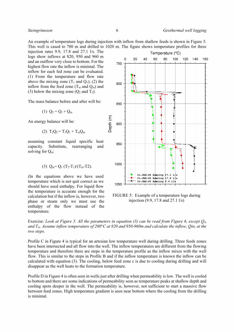
An example of temperature logs during injection with inflow from shallow feeds is shown in Figure 5. This well is cased to 780 m and drilled to 1020 m. The figure shows temperature profiles for three injection rates 9.9, 17.8 and 27.1 l/s. The logs show inflows at 820, 950 and 960 m and an outflow very close to bottom. For the highest flow rate the inflow is minimal. The inflow for each fed zone can be evaluated. (1) From the temperature and flow rate above the mixing zone (T1 and Q1); (2) the inflow from the feed zone (Tin and Qin) and (3) below the mixing zone (Q2 and T2). The mass balance before and after will be:

(1) Q2 = Q1 + Qin An energy balance will be:

(2) T2Q2 = T1Q1 + TinQin assuming constant liquid specific heat capacity. Substitute, rearranging and solving for Qin:

(3) Qin= Q1 (T2-T1)/(Tin-T2). (In the equations above we have used temperature which is not quit correct as we should have used enthalpy. For liquid flow the temperature is accurate enough for the calculation but if the inflow is, however, two phase or steam only we must use the enthalpy of the flow instead of the temperature. Exercise: Look at Figure 5. All the parameters in equation (3) can be read from Figure 6, except Qin and Tin. Assume inflow temperature of 200°C at 820 and 950-960m and calculate the inflow, Qin, at the two steps.

Profile C in Figure 4 is typical for an artesian low temperature well during drilling. Three feeds zones have been intersected and all flow into the well. The inflow temperatures are different from the flowing temperature and therefore there are steps in the temperature profile as the inflow mixes with the well flow. This is similar to the steps in Profile B and if the inflow temperature is known the inflow can be calculated with equation (3). The cooling, below feed zone c is due to cooling during drilling and will disappear as the well heats to the formation temperature. Profile D in Figure 4 is often seen in wells just after drilling when permeability is low. The well is cooled to bottom and there are some indications of permeability seen as temperature peaks at shallow depth and cooling spots deeper in the well. The permeability is, however, not sufficient to start a massive flow between feed zones. High temperature gradient is seen near bottom where the cooling from the drilling is minimal.

FIGURE 5: Example of a temperature logs during injection (9.9, 17.8 and 27.1 l/s)


Knowledge of the formation temperature is important during the drilling in order to decide casing depths, as production casing is typically run into temperatures of at least 230°C and also decide the final depth. The most common way to obtain information on the formation temperature is to measure the temperature build up at the bottom of the well during breaks in the drilling, i.e. if the drilling is stopped over night or over a weekend which is common in low temperature drilling in Iceland. The drilling of high temperature wells is, however, a continuous operation and the drilling not stopped for temperature build-up measurements unless absolutely necessary in order to determine the formation temperature at the planned depth for the production casing. Drilling and water circulation is then stopped and the temperature tool run to bottom to monitor the temperature build up for a short period of time typically 12 hours up to 2 days. Various methods have been developed to extrapolate the temperature build-up data at a certain depth (bottom) to formation temperature. In Iceland we use two semi analytical methods, Horner plot and the Albright method. Both methods assume that the heating is controlled by heat conduction and there is now fluid flow in the well at the measuring depth. The latter method is fairly accurate for heating up histories less than 24 hours but the Horner plot usually requires few days of heating up for accurate determination of the formation temperature. Example of Horner plot data will be shown during the presentation. 3.2. Temperature logs after drilling. Estimation of formation temperatures The heating of geothermal wells after drilling is monitored carefully by regular temperature and pressure logs. The objective is to obtain further information on location of feed zones, to study flow between feed zones and to estimate the size (permeability) of individual feeds. The main objective in analysing the temperature logs after drilling is, however, centre towards the estimation of the temperature of the formations surrounding the well. Low permeability wells will heat slowly over a period of several months as the heating rate is controlled by heat conduction alone and will eventually reach equilibrium temperatures matching the formation temperatures. Example of heating profiles in a low permeable well is shown on Figure 6. The well intersected two warm water aquifers at 175 and 230 m yielding 3 l/s of 25°C water. Cooling zones at 350 and 520 m indicate infiltration of cooling water into the formation but no fluid flow is observed in the temperature logs at these depths and the permeability in the well from 230 m to bottom at 600 m negligible. The well heats rapidly during the first week after drilling and has reached equilibrium temperatures with the formation in the log done six months after drilling. The well was then plugged at 510 m but the formation temperature from there on to bottom can easily be determined using Horner plot or the Albright method. The formation temperature, in the flowing section above 230 m, can, however, not be determined but following constraints are set by the logs.

1. The flowing water cools as it flows upwards the well indicating conductive heat loss. The formation temperature from surface to 230 m depth is therefore lower than the measured temperature in the well.

2. The step in the temperature a 175 m is due to inflow of cooler water at this depth. 3. The surface temperature is expected to be 2°C, the annual mean temperature in the area in

Iceland. Example of temperature logs in a high temperature well is shown in Figure 7. The logs are done over a period of ten years, starting with a log during injection at the end of the drilling process and followed

FIGURE 6: Heating profiles for a low temperature well


by several logs during two moths heating and after six months flow testing of the well. The logging dates are omitted on the graph. The well is drilled through ground water system into a very hot and deep high temperature reservoir. The ground water system was cased and production casing set at 800 m, before the well was drilled to 1804 m. Analyses of the temperature logs are the following:

1. The log during 25 l/s injection (brown asterix) shows that the injection flows to a feed zone at 1795 m. Inspection of the slope of the curve indicates water losses at 1100-1200 m and at 1300-1500 m.

2. The logs during two months heating period show interzonal flow from feed zones at ~1100 m and 1300-1400 m, to the feed zone at 1795 m.

3. The well was not fully heated after two months, when it was stimulated to flow and flow tested for six months.

4. The logs after the flow testing show consistent temperatures for years and are considered to show the formation temperature curve for the well.

5. Comparison of the temperature and the pressure in the well show that water temperature is below the boiling point at all depths.

6. The change in the profile at 800 m is due to fluid convection at the top of the liner.

The temperature logs in well NJ-12 in Figure 7 define fairly accurately the formation temperature at all depths in the well. It should though be emphasized that the estimation of formation temperature for geothermal wells is often more difficult than in the examples in Figures 6 and 7. The most difficult cases are high temperature wells where massive internal flow and boiling in the wells controls the temperature conditions in the well, even though the well is shut in. To interpret the temperature profiles in such wells can be difficult if not impossible. The procedure applied in Iceland for estimating formation temperature is to collect all available temperature logs from the well under study and group them into logs during drilling, during heating after drilling, during flow test and production and monitoring logs. Analyse each group of logs and plot them. For high temperature wells the boiling point depth curve (BPD-curve) is often plotted as a reference as this curve defines the maximum possible formation temperature for the hydrothermal system. If the temperature logs do not define accurately the formation temperature further analyses, interpretation, assumptions or pure guesses are necessary in order to estimate the formation temperature for the well. The main steps in the analyses are as follows:

1) Select logs carried out with the well shut-in and determine what processes in the well are screening away the formation temperature. Interzonal flow is common in permeable wells and screens out the formation temperature

FIGURE 7: Temperature logs in well NJ-12 and formation temperature

FIGURE 8: Formation temperature in a well with internal down flow


from the shallowest feed zone in the production part of the well to the deepest feed. Boiling in very high temperature wells is also common and rising steam bubbles from the boiling region deep in the well will heat the water column higher up in the well as the steam condenses and eventually creates a high pressure and high temperature steam (and gas) cap in the top section of the well suppressing the water level several hundreds of meters into the well.

2) If internal flow controls the well’s temperatures, estimate the formation temperature of sections of the well which are not disturbed by the internal flow i.e. up in the casing and down to the upper most feed zone and in the bottom section below the deepest feed zone. This can be done from logs during heating after drilling, using Horner plot or other extrapolation methods or using the actual measured temperature for these sections when the well has fully recovered after drilling (Figure 8). Connecting the formation temperature curve across the internal flow section can only be done roughly. Steps in the temperature logs (inflow) and the slope of the curve are indicative whether the formation temperature is higher or lower than the measured temperature in the flow section. Analyses of the temperature logs in HE-55 in Figure 8 indicate that the interzonal flow is a down flow from 900 to 2400 m. Minor cooler inflows into the well from 1000 to 1400 m and a small negative slope suggests that the formation temperature is slightly lower than the most resent log. We therefore suggest the pink profile in Figure 8 is a reasonable estimate for a smooth formation temperature curve for well HE-55 from available data. A temperature log during flow or just after a well is being shut-in after flow, often helps analysing the internal flow sections. Well HE-55 is not productive and has never been flow tested. Another example of a down flow in a high temperature well is shown in Figure 9. The logs show down flow in the well from a feed zone at ~1200 m to the bottom of the well. The true temperature of the bottom region of the well can’t be estimated from the heat up logs (green and red curves in Figure 9) but positive slope indicates that it is higher than the well temperatures. The well was flow tested. The initial discharge enthalpy corresponded to water temperatures of ~200°C, in good agreement with the well temperatures before the discharge but after 10-12 hours discharge the bottom feed zone kicked in and the fluid enthalpy rose from 850 to over 2000 kJ/kg indicating very high temperature inflow from the bottom feed zone. It was not possible to run a temperature tool into the well during discharge but a temperature log just after the well was shut-in (black profile in Figure 9) showed temperatures up to 300°C. This temperature value was, however, transient as the down flow from 1100 m starts immediately when the well is closed and pushes the hot fluid back into the bottom feed zone. The log just after discharge confirmed similar formation temperature profile for KJ-11 as for other wells in the Leirbotnar area in Krafla. The profile is shown in Figure 9 as pink line. It shows the existence of a shallow ~200°C hot convective reservoir zone down to ~1200 m and a deeper boiling reservoir from there on to the 2200 m at least, where the temperature rises from ~200°C at 1200 m to 300°C at 1400 m from there on to 345°C, at bottom.

3) High temperature wells often develop during heating after drilling high pressures on wellhead with steam/gas extending from the wellhead and several hundreds of meters down the well. The steam zone temperature is then dictated by the pressure in the steam zone as the boiling point

FIGURE 9: Temperature logs and formation temperature in KJ-11


temperature at that pressure. The steam zone is maintained by continuous boiling and degassing deeper in the well. The temperature in the upper part can often be estimated from temperature logs during drilling, for example by analysing logs done at casing depth but also from the first logs during heating before the well comes under pressure and the steam cap develops. The formation temperature below the boiling steam/gas cap be estimated from Horner plots or other extrapolation methods or directly from temperature logs carried out after the well has fully stabilized in temperature. Examples of temperature logs in a high temperature well under pressure are shown in Figure 10. This is well ÞG-3 at Þeistareykir in north Iceland. The well heated rapidly after drilling in 2006. A log at first casing depth measured on August 23rd suggested very high temperatures close to surface. The first logs during heating after drilling confirmed this and suggested boiling formation temperatures from surface down to at least 700 m. The well came under pressure and developed a steam cap of up to 55 bar pressure and 270°C temperature from the wellhead down to more than one km depth in the well. This steam cap screens out the formation temperature in this interval but the formation controls the temperature below the steam cap. In the case of well ÞG-3, stabilized temperature logs exist as seen in Figure 10. The estimated formation temperature curve is shown in the figure. It is actually made of two boiling point curve corresponding to two boiling reservoir zones. A shallow boiling zone with water level close to surface or even slightly over-pressured, extending to ~700 m depth and a deeper reservoir zone extending to 2.5 or 3 km. The temperature in the deeper zone is also a boiling point curve but the deep reservoir pressures potential is about 20 bar lower than the pressure potential of the upper zone.

We have discussed and showed few examples on how formation temperatures are estimated from temperature logs. We should, however, remember that indications on the formation temperature indications are available from other studies of geothermal wells. The geologists investigate the thermal alteration of the formation from studies of the drill cuttings and cores and define a formation temperature profile based on the alteration minerals seen in the samples. Fluid inclusion studies are also important method to study formation temperatures and finally the geochemists estimate reservoir temperatures based on the chemical content of the reservoir fluid using various geothermometers. These results should be considered in conjunction with the temperature logs when formation temperatures ate estimated. The temperature distribution in geothermal systems is determined by heat and fluid flow (water and steam) through the system. To understand how the system works and set up a conceptual model it is imperative to map the reservoir temperature as accurately as possible. The estimation of the formation temperature is the first step in this direction. Figure 11 shows various types of formation temperature curves in some geothermal wells in Iceland. Each type tells a story on fluid flow conditions in the vicinity of the wells:

FIGURE 10: Temperature logs and formation temperature for well ÞG-3


1. Linear profiles as seen in Figure 11 (Vestmannaeyjar, Þorlakshöfn and Akranes) indicate little or no vertical fluid flow in a low permeability formation. The heat transfer is dominated by heat conduction and the slope of the temperature log, called the geothermal gradient, is determined by the heat conductivity of the formation and the heat flux through

the crust upward to the surface at the location of the well. The average geothermal gradient in the shallowest part of the Earth’s crust is 30°C/km. The gradient of the three linear logs in Figure 11 are much higher or 60 to 140°C/km which is much higher than the world average due to much higher heat flux from volcanic active regions in Iceland.

2. Isothermal formation temperature profiles are found in regions of deep infiltration, circulation, convection, of the fluids. The Kaldársel well is located in a volcanic fracture zone where meteoric water infiltrate to great depths whereas in wells, in Eyjafjörður, Reykjavík and Svartsengi, hydrothermal convection dominates the heat transfer as the fluid mines the heat down to several kilometres depth and pump it up towards the surface. These systems are fractured and their vertical permeability is high. The isothermal formation profiles are typical for all major liquid dominated geothermal reservoirs for temperatures up to 250°C. The steam dominated systems are also isothermal and most of them have a reservoir temperature of 240°C and reservoir pressure of 35 bar.

3. Boiling formation temperature profiles are common in geothermal system with reservoir temperatures in the range of 300°C. These reservoirs are fractured and highly permeable so the heat transfer is dominated by fluid convection and up flow of steam.

4. Temperature reversals are sometimes seen in formation temperature curves (well MG-39 in Figure 11). This is usually explained to be due to horizontal or tilted flow of hot water in the underground. This could be up-flow along a non-vertical fracture or that the well is located in the outflow zone of a geothermal reservoir. Temperature reversal is also seen in cold recharge zones to geothermal reservoirs. This is the explanation to the reversal in well MG-39 and other well sin that area.

FIGURE 11: Various formation temperature profiles for Icelandic geothermal wells. The black curve is the BPD-curve and the point A on the graph is set at 200°C at 1 km depth, which distinguishes between high and low temperature

systems


3.3 Temperature maps of geothermal reservoirs In the preceding chapters we have discussed temperature logs in geothermal wells and how they are analyzed to obtain formation temperature profiles. Plotting these data in a plan view or a section and drawing isothermal contours produces a map showing how the temperature varies within the reservoir and at the reservoir boundary areas. Such maps indicate location of conductive and convective zones inside the geothermal system and divide it into recharge areas, upflow zones and out flow areas. The formation temperatures maps, drawn before any exploitation starts from the reservoir, define the natural thermal state of the reservoir but maps based on temperature data from reservoir under exploitation will reveal temperature changes caused by the production through pressure drawdown, induced fluid recharge and boiling. Temperature maps are very important in the development of conceptual models of geothermal reservoirs. Several examples of temperature maps and cross sections will be shown during presentations at the Short Course but to conclude the discussion here a temperature cross section for the Krafla field in Iceland is shown in Figure 12.

4. PRESSURE LOGS 4.1 Introduction Pressure is an essential parameter in geothermal reservoir studies. It is a property that is tied directly to the fluid. Global pressure variations in the reservoir are the driving force for fluid flow and time variations of the pressure reflect changes in the flow pattern and the fluid reserve of the reservoir. Fluid production/injection will change reservoir pressures in time. Monitoring of reservoir pressures is therefore important to estimate the response of the reservoir to utilization. Pressure is a readily measured parameter and pressure logging is an important tool in geothermal exploration. The logging is carried out in order to study well conditions (fluid flow, boiling etc.), in order to map reservoir pressures and to study transient pressure variations due to fluid injection or production and monitoring of long term pressure changes due to exploitation.

FIGURE 12: West to East Temperature Cross Section for the Krafla field


4.2 Pressure in boreholes. The pressure gradient in a flowing geothermal well will change with depth (z direction) according to the following equation:

(4) dP/dz = (dp/dz)friction + (dP/dz)acceleration + (dP/dz)hydrostatic

If there is no fluid flow in the well the first two terms are zero and the pressure gradient becomes only the hydrostatic (gravity dependent) term or:

(5) dP/dz = (dP/dz)hydrostatic = ρg

where ρ is the density of the fluid (water/steam) and g is earth’s gravitational acceleration. The fluid column in geothermal wells consists of liquid, steam gas and air, media with very different density. The density of each phase will also change with temperature. If, however, we assume isothermal conditions in the well equation can be solved the result being: (6a) P(z) = P0 + ρgz for liquid full well with pressure P0 on the wellhead. or

(6b) P(z) = ρg(z-z0) for well fluid level at depth z0 below the wellhead. The pressure profile of a geothermal well is commonly measured using mechanical Kuster tool or K10 gauges. A hydrostatic calculation of the pressures profile can though be integrated from equation (5) if the temperature dependent density profile of the well is known. There is distinguished between several type of wells depending on their pressure and phase conditions. The main types of static (no-flowing) wells are:

(1) Artesian wells: Liquid water wells with wellhead pressure. These wells will flow spontaneously when opened.

(2) Non Artesian wells (dead wells): Liquid water wells with down-hole water level.

(3) Pressurized high temperature wells: Pressure as high as 80 bar on wellhead and steam/gas cap in the well to a certain depth and water from thereon to bottom. Boiling and degassing at depth maintains the steam/gas cap. The temperature in the cap will be the boiling temperature of water at the cap’s pressure if this is pure steam but lower if the gas fraction increases.

(4) Steam wells: Wells full of steam from top to bottom. Due to the very low density of the steam phase the pressure at bottom is only slightly higher than the wellhead pressure.

Figure 13 shows examples of Artesian and Non-Artesian pressure profiles together with pressure profile in a well with steam/gas cap in the uppermost 200 m of the well.

FIGURE 13: Types of pressure profiles in geothermal wells


The pressure gradient in a static (no-flow) well is controlled by the fluid density, which varies with temperature. The hydrological connection between a geothermal well and the geothermal reservoir is through the feed zones (fractures) intersected by the well. During the drilling operation with water circulation, injection or production the well pressures are varied and controlled by the operators but when the operation is stopped and the well shut-in the pressure in the well changes towards equilibrium with reservoir pressure. In the ideal case of a well with only one feed zone, the pressure at the feed zone depth will change and become equal to the reservoir pressure in short period of time with no flow between the well and the reservoir. The pressure in wells with multiple feed zones will also change towards equilibrium with the reservoir pressure when the well is shut-in after the drilling. The water temperature in the well at the end of drilling and therefore the hydrostatic pressure gradient are different than the temperature and the hydrostatic pressure gradient in the reservoir. This means that the well’s pressure can’t find equilibrium in a way that the pressure matches the reservoir pressure at each feed zone. Usually one feed zone will dominate and therefore the equilibrium point will be close to the “best” feed zone. The mismatch between the temperature and the pressure inside the well and the reservoir pressure will therefore lead to fluid flow between the well and the reservoir. As the well temperatures are, at the end of drilling, always lower than reservoir temperatures the hydrostatic gradient will be higher in the well than in the reservoir. As the cold water column in the well adjusts towards equilibrium with feed zones reservoir pressures the well pressure become lower than the reservoir pressure at the shallower feed zones and higher at the deeper feed zones. This will lead to flow into the well through shallower feed zones and down the well to the deeper feed zones. This is what is called interzonal flow and is seen in all high temperature wells with multiple feed zones. The flow can easily be of the order of tens of l/s in wells with many high permeable feed zones. Example of this is well ÖJ-1 in Figure 5 where the interzonal flow was prominent even during cold water injection into the well. The first response of the well after shut-in after drilling is pressure equilibrium between the well and the reservoir. This usually takes few days. At the same time the well bore fluid heats up accompanied by changes in fluid density. The pressure at the “best” feed zone is, however, fixed at the reservoir pressure. The water column in the well will therefore expand resulting in rising of the water level in the well during the heating and the pressure profiles measured in the well in the heating period will pivot about the depth of the “best” feed zone. Example of the rise in water level in a high temperature well during heating up period is shown in Figure 14 where the water level was at 90 m depth after drilling but rose almost to surface during three weeks of heating.

FIGURE 14: Rising of water level in KJ-21 in Krafla during heating after drilling

FIGURE 15: Pivot point in pressure logs during heating


Information on the feed zones of a well and their relative size is found in the drilling records on circulation losses and gains and in flow meter surveys done during injection and production and last but not least in temperature logs done at the end of drilling, during heating after drilling and during production test. Most wells have several feed zones and in that case, the pivot point is between the feeds, typically closest to the best feed zone. The pivot point is therefore an indicator of the location of best (most permeable) feed zone in wells and determines the reservoir pressure at that depth. Figure 15 show several pressure logs during heating of a well after drilling. The pivot point is at about 800 m and the reservoir pressure at that depth is 62 bars. 6.3. Reservoir pressures. The pivot point, in pressure logs during heating after drilling, determines the reservoir pressure at that specific depth. The next step in the pressure log analyses is to determine or estimate the reservoir pressure profile for the well. This pressure profile can be measured in the well if the temperature profile at the end of the heating period is identical to the formation (reservoir) temperature. That is, however, rare in high temperature wells due to inter zonal flow and boiling. The reservoir pressure profile for the well can then be estimated by hydrostatic extrapolation from the pivot point depth pressure value using the formation temperature curve for the well to determine the water density as a function of depth. Figure 16 shows pressure log from well KJ-14 in Krafla which was drilled in 1980. The pivot point in the well during heating was at 1200 m and the pivot point pressure was 90 bar. The pink curve is the estimated reservoir (initial) pressure based on hydrostatic extrapolation but the red curve is the boiling point depth pressure curve with water level at surface. Estimating the reservoir pressure profile for all wells in the same field is an important step in comparing the pressure values in different wells and different depths and visualizing the pressure distribution in the reservoir. 6.4 Pressure maps. Estimating the reservoir pressure profile for all wells in the same field is an important step in comparing the pressure values in different wells and at different depths and visualizing the pressure distribution in the reservoir. The data are plotted in a similar manner as the formation temperature data i.e. in plan views and cross sections and iso- pressure contours drawn to produce maps showing how the pressures vary within the reservoir. These maps will indicate fluid flow directions in the reservoir in the natural state prior to exploitation and after exploitation starts the pressure maps will show pressure drawdown in the reservoir. Figure 17 shows simulated pressure map for the Nesjavellir field in the natural state. The figure shows high pressures in the recharge zone (upflow-zone) and declining pressures towards north

FIGURE 16: Reservoir pressure curve estimated from the pivot point using

hydrostatic extrapolation

FIGURE 17: The Nesjavellir Geothermal Field. Pressure map at sea

level (~200 m depth)


east. Well locations are shown as black dots and well pressures at sea level depth are given in parenthesis. Several example pressure maps will be shown during the presentations at the “Short Course”. 7. CONCLUDING REMARKS AND RECCOMENDED LITTERATURE This paper has presented a brief description of geothermal well logging for temperature and pressure and the most common interpretation methods. Few general textbooks are available on the subject. The best reference book is probably Geothermal Reservoir Engineering by Malcolm A. Grant and Paul F Bixley. The first edition of the book was published by Academic Press in 1982 but a revised second edition became available 2011. Another booklet is “Geothermal Logging, An Introduction to Techniques and Interpretation”, which was published in Iceland in 1980 and has been used in the annual introductory course at UNU for years. These books are recommended to the participant in the Short Course for further studies of temperature and pressure logs.

geothermal well logging: temperature and · pdf filegeothermal well logging 3...

Documents