geomorphological modelling and mapping of the peru-chile

HAL Id: hal-02464865https://hal.archives-ouvertes.fr/hal-02464865

Submitted on 6 Feb 2020

HAL is a multi-disciplinary open accessarchive for the deposit and dissemination of sci-entific research documents, whether they are pub-lished or not. The documents may come fromteaching and research institutions in France orabroad, or from public or private research centers.

L’archive ouverte pluridisciplinaire HAL, estdestinée au dépôt et à la diffusion de documentsscientifiques de niveau recherche, publiés ou non,émanant des établissements d’enseignement et derecherche français ou étrangers, des laboratoirespublics ou privés.

Distributed under a Creative Commons Attribution - NonCommercial| 4.0 InternationalLicense

Geomorphological modelling and mapping of thePeru-Chile Trench by GMT

Polina Lemenkova

To cite this version:Polina Lemenkova. Geomorphological modelling and mapping of the Peru-Chile Trench by GMT.Polish Cartographical Review, 2019, 51 (4), pp.181-194. �10.2478/pcr-2019-0015�. �hal-02464865�

https://hal.archives-ouvertes.fr/hal-02464865

http://creativecommons.org/licenses/by-nc/4.0/



https://hal.archives-ouvertes.fr

1. Introduction

The geographic study area is located in the Peru-Chile Trench, also known as the Atacama Trench (C. Gambi et al. 2003). It is the longest hadal trench of the Pacific Ocean, stretching 5,900 km from Ecuador to Chile: 6° 00′ S, 81° 50′ W to 39° 00′ S, 75° 00′ W (L.R. Fisher and R.W. Raitt 1962; fig. 1). Considering its total length, the trench covers an area of ca. 590,000 km2 (M.V. Angel 1982). The Peru--Chile Trench is narrower than other trenches of the Pacific Ocean (64 km in width). It is the deepest trench of the South Pacific Ocean, reaching a maximal depth of 8,065 m.

The Peru-Chile Trench was formed by the subduction of the Nazca and Antarctic plates beneath the South American Plate. As can be

understood by its name and location, the trench can be logically divided into two parts: Peru-vian and Chilean. The Chilean part is longer than the Peruvian, stretching in a north–south di-rection along 4,300 km, from -18° S to -56° S. Due to the specific geologic, geotectonic, geo-morphic and climatic settings, the region of the Peru-Chile Trench is exposed to a wide variety of hazardous processes: earthquakes; local tsunamis, generated between the Peru-Chile Trench and the Chilean coast; volcanism, and continent-specific geological hazards: floods, landslides and mass movements, as briefly dis-cussed below. The volcanism intensity can be illustrated by the recently documented tsuna-migenic giant earthquakes: Valdivia, the largest ever recorded (Mw = 9.5), 1960; and Maule (Mw = 8.8), 2010 (E. Contreras-Reyes et al. 2010).

Polish Cartographical ReviewVol. 51, 2019, no. 4, pp. 181–194

DOI: 10.2478/pcr-2019-0015POLINA LEMENKOVA Received: 02.10.2019Ocean University of China Accepted: 09.12.2019College of Marine Geo-sciencesQingdao, Chinaorcid.org/0000-0002-5759-1089 [email protected]

Geomorphological modelling and mapping of the Peru-Chile Trench by GMT

Abstract. The author presents a geospatial analysis of the Peru-Chile Trench located in the South Pacific Ocean by the Generic Mapping Tool (GMT) scripting toolset used to process and model data sets. The study goal is to perform geomorphological modelling by the comparison of two segments of the trench located in northern (Peruvian) and southern (Chilean) parts. The aim of the study is to perform automatic digitizing profiles using GMT and several scripting modules. Orthogonal cross-section profiles transecting the trench in a perpendicular direction were automatically digitized, and the profiles visualized and compared. The profiles show variations in the geomorphology of the trench in the northern and southern segments. To visualize geo-logical and geophysical settings, a set of the thematic maps was visualized by GMT modules: free-air gravity anomaly, geoid, geology and bathymetry. The results of the descriptive statistical analysis of the bathymetry in both segments show that the most frequent depths for the Peruvian segment of the Peru-Chile Trench range from -4,000 to -4,200 (827 recorded samples) versus the range of -4,500 to -4,700 m for the Peruvian segment (1,410 samples). The Peruvian segment of the trench is deeper and its geomorphology steeper with abrupt slopes compared to the Chilean segment. A comparison of the data distribution for both segments gives the following results. The Peruvian segment has the majority of data (23%) reaching 1,410 (-4,500 m to -4,700 m). This peak shows a steep pattern in data distribution, while other data in the neighbouring diapason are significantly lower: 559 (-4,700 m to -5,000 m) and 807 (-4,200 m to -4,400 m). The Chilean segment has more unified data distribution for depths of -6,000 m to -7,000 m. This paper presents GMT workflow for the cartographic automatic modelling and mapping deep-sea trench geomorphology.

Keywords: GMT, mapping, Peru-Chile Trench, submarine geomorphology

Unauthentifiziert | Heruntergeladen 02.02.20 15:49 UTC

https://orcid.org/0000-0002-5759-1089

mailto:[email protected]

182 Polina Lemenkova

The environmental setting of the Peru-Chile Trench is considered as eutrophic with high biological productivity and organic matter on the seafloor (N.C. Lacey et al. 2016). The uni-queness of the biodiversity of the Peru-Chile Trench is notable due to high concentrations

of nutritionally rich organic matter at a depth of 7,800 m, and high nematode densities (C. Gambi et al. 2003).

2. Geographic settings

2.1. Bathymetry

The continental margin of Southern Chile between 36° S and 39° S has an intermediate shelf of 20–30 km in width (D. Völker et al. 2008). The slope has an incline of 2.5–4.0 degrees with irregular-ities: plateaus, slope basins and escarpments as steep as 10 de-grees. The South Chilean slope is dissected by meandering subma-rine canyons connected to the large rivers off the continent.

The Biobío Canyon ends in submarine fans where it enters the trench (T.M. Thornburg and L.D. Kulm 1990). A sinuous axial channel is observed in the Chilean Trench (D. Völker et al. 2008).

It originates from the Chacao Canyon at 41° S, connected to the largest submarine canyon sys-tems of the continental margin (Calle-Calle, Tolten, Biobío and San Antonio Canyons). The Na-zca Plate forms the oceanward bo-undary of the Peru-Chile Trench; it elevates to ca. 100–400 m above the trench and shows parallel geological lineaments. The Nazca Plate has chains of 2-km-high sea mounts that are aligned quasi--parallel to the subduction of the Valdivia and Mocha Fracture Zones (E. Contreras-Reyes et al. 2013; fig. 2). Details of the complexity of the oceanic fracture zones is dis-cussed by E. Contreras-Reyes et al. (2008).

2.2. Tectonics

The Peru-Chile Trench was formed by the subduction of the oceanic crust of the Nazca

Fig. 1. Bathymetric map of the Peru-Chile Trench area. Topographic base map: ETOPO1


183Geomorphological modelling and mapping of the Peru-Chile Trench by GMT

Plate and the Antarctic tectonic plates beneath the South American Plate. The convergence rate of the Nazca Plate is 6.7–6.9 cm/year (J. Geersen 2019). The Mocha crustal block, configured by the Peru-Chile Trench, lies on the Nazca Plate (E. Contreras-Reyes et al. 2010). The complex pro-cesses of the tectonic plate sub-duction in the historical context of the evolution of the Nazca and Antarctic plates are des cribed in relevant works (L.F. Sarmiento--Rojas et al. 2006; V.C. Manea et al. 2017; S.C. Cande and R.B. Leslie, 1986; W.P. Schellart et al. 2006). Central Andes is a typical example of the convergent continental margin where the forearc reflects the in-teraction between the subducting and overriding plates (A.E. Mather et al 2014). The interaction between the Chile Ridge and the continen-tal margin determines the Taitao Triple Junction (46–47° S). The Nazca Plate is subducted beneath the South American Plate, while the Antarctic Plate subducts along an easterly direction (A. Cecioni and V. Pined 2010). The Nazca Plate, adjacent to the Peru-Chile Trench, is located at the boundary of the East Pacific Rise, the fastest--spreading ocean ridge on Earth. It is bordered by the Easter micro-plate and the Juan Fernandez microplate. These include three major seamount chains: Easter Seamount Chain, Nazca Ridge, and Carnegie Ridge (J.P. Bello--González et al. 2018). The earth-quake of 1960 was due to the subduction of the Mocha fracture zone, which caused the rupture of the Nazca Plate (I.L. Cifuentes 1989).

2.3. Geomorphology

The main geomorphic structural units in Chile are Coastal Cordillera, Central Depres-sion and Andean Cordillera. The distinguishing

features of the Peru-Chile Trench include sub-marine ridges, such as Juan Fernández, Copi-apó, Taltal, Nazca, Iquique, O’Higgins Guyot and Eastern Seamount Chain (fig. 2).

The Iquique Ridge is composed of several seamounts surrounded by a shallow seafloor,

Fig. 2. Geologic settings map of the Peru-Chile Trench area



swelling up to 250 km wide (E. Contreras-Reyes, D. Carrizo 2011; see fig. 1). The geomor-phology of the subducted slab in the Peru-Chile Trench region changes from flat to steep along its path beneath the Andes. The region of the Juan Fernandez Ridge subduction beneath the continental margin (27–33° S) correlates with a flat-slab subduction zone (A. Cecioni, V. Pineda 2010). The flat-slab subduction zone is located northwards of the Taitao Triple Junc-tion (J.S. Behrmann et al. 1994). The geo-morphological features of the Chilean Andes are characterized by transverse river valleys separating Coastal from Andean Cordillera (27–33° S). Southwards of 33° S, geologic and geomorphic features in the Peru-Chile Trench change due to the dip of the subduction zone (A. Cecioni, V. Pineda 2010).

2.4. Sedimentation

The system of giant landslides, rock ava-lanches and multiple rotational failures is lo-cated along the coastline within a distance of ca. 650 km and contributes to the sedimenta-tion of the Peru-Chile Trench. There are over 60 large landslides located on the Coastal Cordillera and Atacama Desert adjacent to the Peru-Chile Trench (A.E. Mather et al. 2014). Earthquakes increase sediment thickness as well; for example, in the region of the 1960 earthquake, sediment thickness ranged from ca. 300 to 700 m (R.A. Prince, L.D. Kulm 1975; D. Divins 2003).

Over 50% of the world’s deep-sea trenches are classified as sediment-starved or partly sediment-filled (J. Geersen et al. 2018). The northern part of the Peru-Chile Trench (Peru), is ‘sediment-starved’, while the southern part (Chile) is partly ‘sediment-filled’ (J. Geersen 2019). In response to the sediment loading at the trench, downward deflection plays a crucial role in determining its inlet sediment capacity. Weak and hot oceanic plates show more down-ward deflection at the trench due to sediment loading compared to the old oceanic plates (E. Contreras-Reyes, A. Osses 2010). A weak oceanic plate allows more space for sediment subduction. For the Peru-Chile Trench, larger downward deflection is found along the Chiloé segment (E. Contreras-Reyes et al. 2013). Ac-cording to the sedimentation conditions, the

Peru-Chile Trench can be divided into two main provinces: the main sediment-free prov-ince (8–32° S) and the sedimentary province (33–57° S; see D.E. Hayes 1966). The margin off Isla de Chiloé is characterized by a largely sedimented segment of the Peru-Chile Trench caused by the turbidite deposits (E. Contreras-Reyes et al. 2007). The region close to the Taitao Triple Junction is nearly devoid of sedi-ment and displays rapid narrowing of the forearc region (S.C. Cande et al. 1987).

3. Materials and methods

The goal of the current study is to compare two segments of the trench located in northern (Peruvian) and southern (Chilean) parts through geomorphological modelling by cross-section profiles. The study aim is to perform automatic digitizing of the profiles using GMT and several scripting modules. The orthogonal cross-sec-tion profiles transecting the trench in a perpen-dicular direction were automatically digitized, and the profiles visualized and compared. There are documented attempts to study the Peru-Chile Trench by drawing vertical profiles to study the variability of the data along the transects (J.M. Zeigler et al. 1957). However, along with the rapid development of advanced technologies in IT and the improvement of data analysis algorithms and automatization, ap-proaches to studying geomorphology have developed correspondingly. The application of advanced scripting towards data modelling (P. Lemenkova 2019b) enables complex ana-lysis of the bathymetric data, advance map-ping, automated digitizing and visualization to be performed. This study presents the metho-dological experience of using Generic Mapping Tools (GMT) for processing, modelling and map-ping geodata, aimed at visualizing the geo-morphology of the Peru-Chile Trench.

The methodology is based on GMT (P. Wessel and W.H.F. Smith 1998; P. Wessel et al. 2013). A principal strategy of GMT, and its fundamen-tal difference from classical GIS software, lies in its scripting approach. Thus, to produce a map, to visualize geodata and perform modelling, a cartographer needs to write a code similar to programming lines in principle (as demon-strated below). A combined sequence of such codes creates a script which facilitates creating maps or graphs.



Since the precision of the geodata is an im-portant issue in cartographic mapping, as dis-cussed in previous works (e.g. for bathymetric data (W.H.F. Smith 1993) and for gravity (P. Wes-sel, A.B. Watts 1988)), high quality raster grids were selected as a background for mapping: ETOPO1 (1 min resolution global data set) and gravity raster grid public data sets from Scripps Institution of Oceanography (SIO).

ETOPO1 is based on the horizontal datum WGS 84 geographic, with bathymetry estimated from satellite altimetry. The vertical uncertainty of the ETOPO1 elevations exceeds the differ-ences between the vertical datums near the sea level (< 1 m), which makes this data set reliable. Mapping and visualization of the raster grids was based on the existing algorithms of GMT modules used for current research. The most important codes are explained below in the relevant subsections.

3.1. Bathymetric and geologic mapping

The technical methodology for the thematic mapping is based on using a GMT scripting approach where each line of the code is respon-sible for adding certain cartographic elements on the map or for manipulations with the raster data. Thus, the bathymetric map (fig. 1) is made using the following sequence of the most es-sential GMT codes:

Step-1. Extracting a subset of ETOPO1m for the Peru-Chile area. Format: -R0/360/-90/90; here, 0°00 S to -55°00 S, 90° W to 60° W; through ‘grdcut’ GMT module: grdcut earth_relief_01m.grd -R270/300/-55/0 -Gpct_relief.nc

Step-2. Making the colour palette is done using the following code: gmt makecpt -Cgeo.cpt -V -T-8000/7000 > pctocean.cpt

Step-3. Visualizing the raster image is done by the GMT ‘grdimage’ module through this code: gmt grdimage pct_relief.nc -Cpctocean.cpt -R270/300/-55/0 -JM4.5i -P -I+a15+ne0.75 -Xc -K > $ps

Step-4. Adding shorelines was done using GMT ‘grdcontour’ module: gmt grdcontour pct_relief.nc -R -J -C1000 -W0.2p -O -K >> $ps

Likewise, adding cartographic elements on the map is done through the GMT module ‘psbasemap’: grid with major and minor lines, scale, directional rose, colour legend. Adding annotations is done through the GMT module

‘pstext’. The geological lineaments are added using GMT module ‘psxy’ as in the following examples:

gmt psxy -R -J ophiolites.gmt -Sc0.2c -Gma-genta -Wthinnest -O -K >> $ps

gmt psxy -R -J volcanoes.gmt -St0.4c -Gred -Wthinnest -O -K >> $ps

gmt psxy -R -J ridge.gmt -Sf0.5c/0.2c+l+t -Wthinnest,black -Ggreen -O -K >> $ps

3.2. Geoid modelling

The modelling geoid map (fig. 3) is based on the fundamental principle of the geoid, which is the equipotential surface of the Earth’s gravity field that best fits the undisturbed mean sea level (F.W. Gauss 1828).

In other words, the geoid model shows the level surface of the Earth’s gravity field that can be taken as a reference for the standardized elevation height systems into a global system. The geoid was modelled using the following GMT key sequence of codes stepwise:

Step-1. A colour palette table from the grid raster is generated using the following code:

gmt grd2cpt geoid.egm96.grd -Crainbow > geoid.cpt

Step-2. A geoid image with shading is gene-rated at the 2nd step:

gmt grdimage geoid.egm96.grd -I+a45+nt1 -R270/300/-55/0 -JM4.5i -Cgeoid.cpt -P -K > $ps

Here the ‘geoid.egm96.grd’ is an input file; ‘-I+a45’ shows the illumination of the grid, ‘-R270/300/-55/’ shows the coordinates squares of the taken area in W-E-S-N direction; ‘-JM4.5i’ means a Mercator projection and the dimen-sions of the map of 4.5 inches; ‘-Cgeoid.cpt’ means the colour palette taken; ‘-P’ means a port-rait orientation of the map; ‘-K’ means a conti-nuation of the codes.

Step-3. The base map elements (grid, title, coastlines) are added:

gmt pscoast -R -J -P -V -W0.25p -Df -B+t”Geoid regional model: Peru-Chile Trench area” -Bxg-3f4a4 -Byg3f2a4 -O -K >> $ps

In this code, the meaning of ‘-Bxg3f4a4 -Byg3f2a4’ is the grid density (major lines every 3, minor lines every 4, annotations every 4 for the latitude coordinates, with the same system for longitude). ‘-W0.25p’ means the thickness of the plotted lines (here: very thin ones, 0.25 points).



Step-4. The geoid contour is added through the following code snippet:

gmt grdcontour geoid.egm96.grd -R -J -C2 -A5 -Wthinnest,dim-gray -O -K >> $ps

Here ‘geoid.egm96.grd’ is the input file from which the data were taken; ‘-Wthinnest, dimgray’ is the aesthetics of the lines; ‘-A5’ means that the lines are annotated every 5th one.

3.3. Free-air gravity modelling

A combination of several GMT modules is used for mapping geo-morphological profiles based on the methodology of the GMT (P. Wes-sel et al. 2019). As noted (H. Amin et al. 2019), the Earth’s gravity field is subject to temporal varia-tions. Therefore, the geoid model is not a static surface. Temporal changes in the Earth’s gravity field are attributed to the move-ment of the water masses within the Earth’s thin fluid envelope that can be revealed using geodetic modelling (J.Wahr et al. 1998). Hence, the sea level change and mass redistribution affect the equi-potential surfaces in the Earth’s gravity field. Therefore, the marine free-air gravity modelling should be based on the most updated available grid data. Current re-search relies on such existing raster data sets (W.H.F. Smith, D.T. Sand-well 1995; D.T. Sandwell et al., 2014) visualized as gravity mo-dels (fig. 4). The technical metho-dology of the free-air modelling for the Peru-Chile Trench area and western South America is based on the following GMT codes (the most important codes have been selected and the minor code lines used mainly for cartographic aesthetics were skipped):

Step-1. The subset of the img file in Mercator projection is extracted using the following code: img2grd

Fig. 3. Geoid model map of the Peru-Chile Trench area



grav_27.1.img -R270/300/-55/0 -Ggra-vPCT.grd -T1 -I1 -E -S0.1 -V

Step-2. A colour palette table from the grid is generated for the gravity modelling: gmt grd2cpt gravPCT.grd -Crainbow > gravPCT.cpt

Step-3. The gravity image with shading is visualized through this code: gmt grdimage gravpCT.grd -I+a45+nt1 -R270/300/-55/0 -JM4.5i -CgravPCT.cpt -P -K > $ps

Step-4. Some base map parame-ters and elements are added (grid, title, coastline): gmt pscoast -R -J -P -V -W0.25p -Df -B+t”Marine free-air gravity anomaly for the Peru–Chile Trench area” -Bxg3f2a4 -Byg3f2a4 -O -K >> $ps

Step-5. A colour legend is added through this code: gmt psscale -R -J -CgravPCT.cpt -DjBC+o0.0c/-2.0c+ w12c/0.5c+h -Baf+l”Marine free-air gravity anomaly colour scale” -I0.2 -By+lmGal -O -K >> $ps

Here, the -’DjBC+o0.0c/-2.0c+w-12c/0.5c+h’ snippet shows the bot-tom centre alignment , ‘0.0c/-2.0c’ offset on ‘y’ scale 2 cm to the left, ‘w12c/0.5c+h’ means a 12 cm height and 0.5 cm the width of the colour legend, and ‘h’ means horizontal stretching (that is, the legend is placed below the main map). The output free-air marine gravity map of the Peru-Chile Trench region is visualized in figure 4.

3.4. Automated digitizing of the profiles

Before the computer era, manual visualization of the profiles was the only possibility for geoscientists to model geomorphic features, as pre-sented, for example, in J.M. Zeigler et al. (1957) who studied the Peru--Chile region by profiling, and using the methods available at that time. The rapid development of the computerization in geosciences, together with machine learn-ing tools, presented the possibility of semi--automatically digitizing bathymetric isolines in ocean topographic maps. Experience of auto-

matization is reported by H.W. Schenke, P. Le-menkova (2008) in their research on con verting raster bitmap images to vector lines. The cur-rent study presents a more advanced step in cartographic automatization using the metho-

Fig. 4. Gravimetry model map of the Peru-Chile Trench area



dology of GMT (P. Wessel, W.H.F. Smith 2018). The principle approach consists of automatic machine-based digitizing of the pro-files, then deriving attribute tables for xy coor-dinates and z values (depths) for each sample point. Technically, the GMT code for automatic digitizing of the Peru-Chile Trench is as follows:

Step-1. Two points are selected by the coordi-nated (here: along the Peruvian segment) and saved to the table (here: trenchPCTn.txt) cat << EOF > trenchPCTn.txt 279.1 -9.0 282.4 -14.0 EOF

Step-2. The line is plotted using this code: gmt psxy -Rpct_relief.nc -J -W2p,yellow trenchPCTn.txt -O -K >> $ps

Fig. 5. Two segments with digitized profiles: Peruvian (north) and Chilean (south)



Step-3. The points (first and last ones) are visualized: gmt psxy -R -J -Sc0.15i -Gyellow trenchPCTn.txt -O -K >> $ps

Step-4. The cross-track profiles 400 km long, spaced 20 km apart, sampled every 2 km are generated: gmt grdtrack trenchPCTn.txt -Gpct _relief.nc -C400k/2k/20k+v -Sm+sstackPCTn.txt > tablePCTn.txt gmt psxy -R -J -Wthin,yellow tablePCTn.txt -O -K >> $ps

Step-5. Upper/lower values encountered as an envelope are shown: gmt convert stackPCTn.txt -o0,5 > envPCTn.txt gmt convert stackPCTn.txt -o0,6 -I -T >> envPCTn.txt

After that the profiles are automatically digi-tized as presented in figure 5. The red line shows the Chilean (southern) segment, the yellow line shows the Peruvian (northern) segment. The table for the statistical analysis of the frequency of depths is then analyzed in the following step.

3.5. Statistical analysis of the profiles through histograms

The statistical analysis applied specifically for the hadal trenches comprises a vast variety of methods and approaches. In this research, the histograms were selected to show the fre-quency of the data distribution and to visualize the repeatability of the maximal depths for the two segments of the Peru–Chile Trench. Tech-nically, the methodology of the histogram plotting is summarized by the following code: gmt pshi-stogram tablePCTn.txt -i4 -R-7000/6/0/25 -JX4.8i/2.4i Bpxg1000a1000f100+l”Bathymetry (m)” -Bpyg5a5f2.5+l”Frequency”+u” %” -Bsyg2.5 -BWSne+t”Histogram of the bathymetry across Peruvian (A) segment”+gsnow1 -Glightsteel-blue1 -D+f7p,Times-Roman,black -L0.1p,dimgray -Z1 -W250 -N0+pred -N1+pgreen -N2+pblue -K > $ps

Here, ‘-JX4.8i/2.4i’ shows the dimension of the plotted graph, ‘ablePCTn.txt’ is the source data table from which the columns are taken. This table is generated automatically during the previous step by the GMT automatic digitizing profiles. Using data from this table, the histo-gram bins are then calculated and plotted. The ‘echo’ Unix program is used to add selected annotations: echo “-6700 22.5 A” | gmt pstext -R -J -F+jBL+f15p,black -Gfloralwhite -W0.5p -O -K >> $ps

4. Results

In this study, GMT-based automatic digitizing was used to visualize geomorphic variations of the Peru-Chile Trench in two different parts: Peruvian and Chilean. Furthermore, gravitatio-nal and geoid modelling, bathymetric and geo-logic mapping were performed using sequential coding of the GMT modules, as is briefly dis-cussed in the ‘Materials and methods- section’. A GMT-based statistical data assessment for the geomorphic variations of the Peru-Chile Trench is presented as visualized histograms. The workflow can be implemented into similar future works for data analysis aimed at the submarine geomorphic modelling of the hadal trenches.

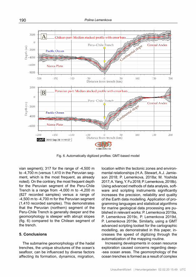
Findings in the automatic digitizing of the transect profiles, visualized as two segments (fig. 6) are as follows: the Chilean trench’s geo-morphology has deeper bathymetry and steeper gradient slope on the Nazca Plate (fig. 6A); on the contrary, the Peruvian segment of the trench (fig. 6B, below) demonstrates a gentler landform on the oceanward side. The compar-ison of the histograms on bathymetry in both segments shows that the Peruvian segment has shallower depths with the maximal reaching -6,500 m, while the Chilean segment reaches -7,800 m in depth (fig. 7). The frequency of the depth records shows the following results: the Chilean segment has more unified data distri-bution for the depth range of -6,000 m to -7,000 m with the following number of sample points: 86, 88, 88, 72. For the same depth diapa-son, the Peruvian part has 56 and 84 samples, respectively. A comparison of the highest fre-quency of the data for both segments shows: the Peruvian segment has the majority of the data (23%) reaching 1,410 samples (-4,500 m to -4,700 m are the most frequent values for the Peruvian segment of the trench). It shows a peak of all data with a very steep pattern in data distribution. Other data in the neighbouring diapason are significantly lower: 559 samples (-4,700 to -5,000 m) and 807 (-4,200 to -4,400 m) for the Peruvian segment.

At the same time, the Chilean segment has more even data distribution. Taking a look at the same data range: only 205 samples for the range -4,700 m to -5,000 m (versus 559 for the Peruvian segment); 731 for the range of -4,200 m to -4,400 m (versus 807 for the Peru-



vian segment); 317 for the range of -4,500 m to -4,700 m (versus 1,410 in the Peruvian seg-ment, which is the most frequent, as already noted). On the contrary, the most frequent depth for the Peruvian segment of the Peru-Chile Trench is a range from -4,000 m to -4,200 m (827 recorded samples) versus a range of -4,500 m to -4,700 m for the Peruvian segment (1,410 recorded samples). This demonstrates that the Peruvian (northern) segment of the Peru-Chile Trench is generally deeper and the geomorphology is steeper with abrupt slopes (fig. 6) compared to the Chilean segment of the trench.

5. Conclusions

The submarine geomorphology of the hadal trenches, the unique structures of the ocean’s seafloor, can be influenced by diverse factors affecting its formation, dynamics, migration,

location within the tectonic zones and environ-mental relationships (H.A. Stewart, A.J. Jamie-son 2018; P. Lemenkova, 2018a; M. Yoshida 2017; A. Yang, Y. Fu 2018; P. Lemenkova, 2018b). Using advanced methods of data analysis, soft-ware and scripting instruments significantly increases the precision, reliability and quality of the Earth data modelling. Application of pro-gramming languages and statistical algorithms for marine geological data processing are pu-blished in relevant works: P. Lemenkova 2019a, P. Lemenkova 2019c, P. Lemenkova 2019d, P. Lemenkova 2019e. Similarly, using a GMT advanced scripting toolset for the cartographic modelling, as demonstrated in this paper, in-creases the speed of digitizing through the automatization of the mapping routine.

Increasing developments in ocean resource exploration caused concerns regarding deep--sea ocean areas. The geomorphology of the ocean trenches is formed as a result of complex

Fig. 6. Automatically digitized profiles: GMT-based model



environmental processes in the ocean eco-systems. Several studies have revealed deep interconnections between the biodiversity of the ocean and the geospatial settings of the ecosystems: geology (sediments, tectonics, stratigraphy), bathymetry (depths), geomorpho-logy (shape) and oceanology (deep currents). Various publications have reported deep ocean

slab dynamics and tectonics (e.g. A.J. Oakley et al. 2008; A. Heuret, S. Lallemand 2005), deep ecosystems functioning and develop-ment (B.H. Robison 2004, 2009; K.J. Osborn et al. 2009; M.J. Costello et al. 2006; M.R. Clark et al. 2009 2010), marine thematic mapping (I.A. Suetova et al. 2005). Several attempts have been made so far to study the correlation

Fig 7. Histograms on the statistical analysis of the bathymetric data distribution



between various factors involved in the func-tioning of the ocean. However, there are certain limitations in these studies mostly caused by the study object: submarine trenches are the least reachable landform on the Earth that require significant application of numerical modelling, machine learning, remote sensing and GIS cartographic tools.

Existing techniques for modelling deep-sea trenches mostly identify relations and processes among the tectonic slabs, depths and seismi-city (C.R. Ranero et al. 2005), tectonic slab subduction and migration (C. Kincaid, P. Olson 1987), slab dynamics and rheology (B. Kaus, T.W. Becker 2008). These and other studies do not discuss geomorphic variations in the trench structure in great detail, but rather focus on geological issues. From the marine geo-

science perspective, insufficient research into deep-sea trenches is caused by limited access to hadal trenches, limitations in methodolog-ical techniques and constraints in the usage of GIS plugins for spatial modelling. Taking the aspect of machine learning and GMT algorithms into account, precision and accuracy in oceano-logical modelling, as well as visualization of oceanographic big data sets, increase signifi-cantly. They also broaden the perspective of marine research to multi-disciplinary level. Hence, this paper presents a contribution to-wards the development of advanced cartogra-phic methods of data processing, visualization and modelling. This technical paper has a me-thodological character aimed at presenting GMT workflow and approaches for the carto-graphic audience.

Literature

Amin H., Sjöberg L.E., Bagherbandi M., 2019, A global vertical datum defined by the conventional geoid potential and the Earth ellipsoid parameters. “Jour-nal of Geodesy” Vol. 93, no. 10, pp. 1943–1961. https://doi.org/10.1007/s00190-019-01293-3

Angel M.V., 1982, Ocean trench conservation. “En-vironmentalist” Vol. 2, pp.1–17.

Behrmann J.S., Leslie S.D., Cande S.C., 1994, ODP Leg 141 Scientific Party. Tectonics and geology of spreading ridge subduction at the Chile Triple Junction: A synthesis of results along from Leg 141 of the Ocean Drilling Program. “Geologische Rundschau” Bd. 83, pp. 832–852.

Bello-González J.P., Contreras-Reyes E., Arriagada C., 2018, Predicted path for hotspot tracks off South America since Paleocene times: Tectonic implications of ridge-trench collision along the Andean margin. “Gondwana Research” Vol. 64, pp. 216–234. DOI:10.1016/j.gr.2018.07.008+

Cande S.C., Leslie R. B., 1986, Late Cenozoic tec-tonics of the southern Chile Trench. “Journal of Geophysical Research” Vol. 91, pp. 471–496.

Cecioni A., Pineda V., 2010, Geology and geomor-phology of natural hazards and human-induced disasters in Chile. “Developments in Earth Surface Processes” Vol. 13, pp. 379–413. DOI: 10.1016/S0928-2025(08)10018-9

Cifuentes I.L.,1989, The 1960 Chilean earthquakes. “Journal of Geophysical Research” Vol. 94, pp. 665–680.

Clark M.R., Rowden A.A., Schlacher R., Williams A., Consalvey M., 2010, The ecology of seamounts: structure, function, and human impacts. “Annual Review of Marine Science” Vol. 2, pp. 253–278. DOI: 110.1146/annurev-marine-120308-081109

Contreras-Reyes E., Carrizo D., 2011, Control of high oceanic features and subduction channel on earthquake ruptures along the Chile-Peru subduc-tion zone. “Physics of the Earth and Planetary Interiors” Vol. pp. 186, 49–58. DOI: 10.1016/j.pepi. 2011.03.002

Contreras-Reyes E., Jara J., Maksymowicz A., Wein-rebe W., 2013, Sediment loading at the southern Chilean trench and its tectonic implications. “Jour-nal of Geodynamics” Vol. 66, pp. 134–145. DOI: 10.1016/j.jog.2013.02.009

Contreras-Reyes E., Osses A., 2010, Lithospheric flexure modeling seaward of the Chile trench: im-plications for oceanic plate weakening in the Trench Outer Rise region. “Geophysical Journal Interna-tional” Vol. 182, no.1, pp. 97–112. DOI: 10.1111/ j.1365-246X.2010.04629.x

Contreras-Reyes E., Flueh E.R., Grevemeyer I., 2010, Tectonic control on sediment accretion and sub-duction off south-central Chile: implications for coseismic rupture processes of the 1960 and 2010 megathrust earthquakes. “Tectonics” Vol. 29, no. 6. DOI: 10.1029/2010TC002734

Contreras-Reyes E., Grevemeyer I., Flueh E.R.M., Scherwath M., Heesemann M., 2007, Alteration of the subducting oceanic lithosphere at the southern central Chile trench-outer rise. “Geochemistry Geo-physics Geosystems” Vol. 8, Q07003. DOI: 10. 1029/2007GC001632.

Contreras-Reyes E., Grevemeyer I., Flueh E.R., Rei-chert C., 2008, Upper lithospheric structure of the subduction zone offshore southern Arauco Pe-ninsula, Chile at -38°S. “Journal of Geophysical Research” Vol. 113, B07303, DOI: 10.1029/ 2007JB005569.



Costello M.J., Berghe, van den E., 2006, Ocean bio-diversity informatics: a new era in marine biology research and management. “Marine Ecology – Progress Series” No. 316, pp. 203–214. DOI: 10.3354/ meps316203

Divins D., 2003, Total sediment thickness of the world’s oceans and marginal seas. Boulder, CO. NOAA National Geophysical Data Center. http://www.ngdc.noaa.gov/mgg/sedthick/sedthick.html

Fisher R.L., Raitt R.W., 1962, Topography and struc-ture of the Peru-Chile trench. “Deep-Sea Research” Vol. 9, pp. 424–443.

Gambi C., Vanreusel A., Danovaro R., 2003, Biodi-versity of nematode assemblages from deep-sea sediments of the Atacama Slope and Trench (South Pacific Ocean). “Deep-Sea Research I” No. 50, pp. 103–117.

Gauss F.W., 1828, Bestimmung des Breitenunter-schiedes zwischen den Sternwarten von Göttingen und Altona durch Beobachtungen am Ramsden-schen Zenithsector. Göttingen: Vanderschoeck und Ruprecht, pp. 48–50.

Geersen J., 2019, Sediment-starved trenches and rough subducting plates are conducive to T tsunami earthquakes. “Tectonophysics” No. 762, pp. 28–44. DOI: 10.1016/j.tecto.2019.04.024

Geersen J., Voelker D., Behrmann J.H., 2018, Oceanic trenches. In: Submarine Geomorphology. Cham: Springer, pp. 409–424.

Hayes D.E.,1966, A geophysical investigation of the Peru-Chile Trench. “Marine Geology” Vol. 4, no. 5, pp. 309–351. DOI: 10.1016/0025-3227(66)90038-7

Heuret A., Lallemand S., 2005, Plate motions, slab dynamics and back-arc deformation. “Physics of the Earth and Planetary Interiors” Vol. 149, pp. 31–51. DOI: 10.1016/j.pepi.2004.08.022

Kaus B., Becker T.W., 2008, A numerical study on the effects of surface boundary condition and rheology on slab dynamics. “Bollettino di Geofisica Teorica ed Applicata” Vol. 49, no. 2, pp. 177–181.

Kincaid C., Olson P., 1987, An experimental study of subduction and slab migration. “Journal of Geo-physical Research” Vol. 92, pp. 13832–13840.

Lacey N.C., Rowden A.A., Clark M.R., Kilgallen N.M., Linley T., Mayor D.J., Jamieson A.J., 2016, Com-munity structure and diversity of scavenging amphi-pods from bathyal to hadal depths in three South Pacific Trenches. “Deep-Sea Research I” No. 111, pp. 121–137. DOI: 10.1016/j.dsr.2016.02.014

Lemenkova P., 2018a, R scripting libraries for com-parative analysis of the correlation methods to identify factors affecting Mariana Trench forma-tion. “Journal of Marine Technology and Environ-ment” Vol. 2, pp. 35–42. DOI: 10.6084/m9.figshare. 7434167

Lemenkova P., 2018b, Factor analysis by R pro-gramming to assess variability among environmen-tal determinants of the Mariana Trench. “Turkish

Journal of Maritime and Marine Sciences” Vol. 4, pp. 146–155. DOI: 10.6084/m9.figshare.7358207

Lemenkova P. 2019a, Statistical analysis of the Ma-riana Trench geomorphology using R programming language. “Geodesy and Cartography” Vol. 45, no. 2, pp. 57–84. DOI: 10.3846/gac.2019.3785

Lemenkova P., 2019b, An empirical study of R appli-cations for data analysis in marine geology. “Mari-ne Science and Technology Bulletin” Vol. 8, no. 1, pp. 1–9. DOI: 10.33714/masteb.486678

Lemenkova P., 2019c., Processing oceanographic data by Python libraries NumPy, SciPy and Pan-das. “Aquatic Research” Vol. 2, pp. 73–91. DOI: 10.3153/AR19009

Lemenkova P., 2019d, Testing linear regressions by StatsModel Library of Python for oceanological data interpretation. “Aquatic Sciences and Engineering” Vol. 34, pp. 51–60. DOI: 10.26650/ASE2019547010

Lemenkova P., 2019e, Numerical data modelling and classification in marine geology by the SPSS statistics. “International Journal of Engineering Tech-nologies” Vol. 5, no. 2, pp. 90–99. DOI: 10.6084/m9.figshare.8796941

Manea V.C., Manea M., Ferrari L., Orozco-Esquivel T., Valenzuela R.W., Husker A., Kostoglodov V., 2017, A review of the geodynamic evolution of flat slab subduction in Mexico, Peru, and Chile. “Tec-tonophysics” No. 695, pp. 27–52. DOI: 10.1016/j.tecto.2016.11.037

Mather A.E., Hartley A.J., Griffiths J.S., 2014, The giant coastal landslides of Northern Chile: Tecto-nic and climate interactions on a classic conver-gent plate margin. “Earth and Planetary Science Letters” No. 388, pp. 249–256. DOI: 10.1016/j.epsl.2013.10.019

Oakley A.J., Taylor B., Moore G.F., 2008, Pacific plate subduction beneath the central Mariana and Izu--Bonin fore-arcs: new insights from an old margin. “Geochemistry Geophysics Geosystems” Vol. 9. DOI: 10.1029/2007GC001820

Osborn K.J., Haddock S.H.D., Pleijel F., Madin L.P., Rouse G.W., 2009, Deep-sea, swimming worms with luminescent ‘bombs’. “Science” Vol. 325, 964. DOI: 10.1126/science.1172488

Prince R.A., Kulm L.D., 1975, Crustal rupture and the initiation of imbricate thrusting in the Peru-Chile Trench. “GSA Bulletin” Vol. 86, no. 12, pp. 1639–1653.

Ranero C.R., Villaseor A., Morgan Ph.J., Wdinrebe W., 2005, Relationship between bending-faulting at trenches and intermediate-depth seismicity. “Geo-chemistry, Geophysics, Geosystems” Vol. 6. DOI: 10.1029/2005GC000997

Robison B.H., 2004, Deep pelagic biology. “Journal of Experimental Marine Biology and Ecology” No. 300, pp. 253– 272. DOI: 10.1016/j.jembe.2004.01.012

Robison B.H., 2009, Conservation of deep pelagic bio-diversity. “Conservation Biology” Vol. 23, pp. 847–858. DOI: 10.1111/j.1523-1739.2009.01219.x


http://www.ngdc.noaa.gov/mgg/sedthick/sedthick.html

http://www.ngdc.noaa.gov/mgg/sedthick/sedthick.html


Sandwell D.T., Müller R.D., Smith W.H.F., Garcia E., Francis R., 2014, New global marine gravity model from CryoSat-2 and Jason-1 reveals buried tectonic structure. “Science” Vol. 346, no. 6205, pp. 65–67.

Sarmiento-Rojas L.F., Van Wess J.D., Cloetingh S., 2006, Mesozoic transtensional basin history of the Eastern Cordillera, Colombian Andes: inferences from tectonic models. “Journal of South American Earth Sciences” Vol. 21, pp. 383–411.

Schellart W.P., Lister G.S., Toy V.G., 2006, A Late Cretaceous and Cenozoic reconstruction of the Southwest Pacific region: tectonics controlled by subduction and slab rollback processes. “Earth Review” Vol. 76, pp. 191–233.

Schenke H.W., Lemenkova P., 2008, Zur Frage der Meeresboden-Kartographie: Die Nutzung von AutoTrace Digitizer für die Vektorisierung der bathymetrischen Petschora-See Daten in der Petschora-See. “Hydrographische Nachrichten” Bd. 25, H. 81, pp. 16–21. DOI: 10.6084/m9.fig-share.7435538

Smith W.H.F., 1993, On the accuracy of digital bathy-metric data. “Journal of Geophysical Research” Vol. 98, no. B6, pp. 9591–9603.

Smith W.H.F., Sandwell D.T., 1995, Marine gravity field from declassified Geosat and ERS-1 altimetry, “EOS Transactions American Geophysical Union” Vol. 76, Fall Mitting Suppl, F156.

Stewart H.A., Jamieson A.J., 2018, Habitat hetero-geneity of hadal trenches: Considerations and implications for future studies. “Progress in Oceano-graphy” Vol. 161, pp. 47–65. DOI: 10.1016/j.poce-an.2018.01.007

Suetova I.A., Ushakova L.A., Lemenkova P., 2005, Geoinformation mapping of the Barents and Pechora Seas. “Geography and Natural Resources” Vol. 4, pp. 138–142. DOI: 10.6084/m9.figshare.7435535

Thornburg T.M., Kulm, L.D., 1990, Submarine-fan development in the southern Chile Trench: a dy-namic interplay of tectonics and sedimentation. “Geological Society of America. Bulletin.” Vol. 102, pp. 1658–1680.

Völker D., Reichel T., Wiedicke M., Heubeck C., 2008, Turbidites deposited on Southern Central Chilean seamounts: Evidence for energetic tur-bidity currents. “Marine Geology” Vol. 251, no. 1-2, pp. 15–31. DOI: 10.1016/j.margeo.2008.01.008

Wahr J., Molenaar M., Bryan F., 1998, Time variability of the Earth’s gravity field: hydrological and oce-anic effects and their possible detection using GRACE. “Journal of Geophysical Research” Vol. 103, pp. 30205–30229.

Wessel P., Smith W.H.F., 1998, New, improved ver-sion of the generic mapping tools released. “EOS Transactions American Geophysical Union” Vol. 79, p. 579.

Wessel P., Smith W.H.F., Scharroo R., Luis J.F., Wobbe F., 2013, Generic mapping tools: improved version released. “EOS Transactions American Geophysical Union” Vol. 94, no. 45, pp. 409–410. DOI: 10.1002/2013EO450001

Wessel P., Smith W.H.F., 2018, The generic map-ping tools. Version 4.5.18 Technical reference and cookbook (Computer software manual). U.S.A.

Wessel P., Smith W.H.F., Scharroo R., Luis J., Wob-be F., 2019, The generic mapping tools. GMT man pages. Release 5.4.5 (Computer software manual). U.S.A.

Wessel P., Watts A.B., 1988, On the accuracy of ma-rine gravity measurements. “Journal of Geophysical Research” Vol. 93, pp. 393–413.

Yang A., Fu Y., 2018, Estimates of effective elastic thickness at subduction zones. “Journal of Geo-dynamics” No. 117, pp. 75–87. DOI: 10.1016/j.jog.2018.04.007

Yoshida M., 2017, Trench dynamics: Effects of dy-namically migrating trench on subducting slab morphology and characteristics of subduction zones systems. “Physics of the Earth and Plan-etary Interiors” No. 268, pp. 35–53. DOI: 10.1016/j.pepi.2017.05.004

Zeigler J.M., Athearn W.D., Small H.,1957, Profiles across the Peru-Chile Trench. “Deep-Sea Re-search” Vol. 4, pp. 238–249. DOI: 10.1016/0146-6313(56)90056-9


geomorphological modelling and mapping of the peru-chile

Documents