Hydrological and Geomorphological Processes of an

extreme Flood in the Rio San Francisco Valley, South Ecuador

Harald Honer

Diplomarbeit unter der Leitung von Prof. Dr. Markus Weiler Freiburg im Breisgau, Februar 2010

Harald Honer

Hydrological and Geomorphological Processes of an extreme Flood in the Rio San Francisco Valley,

South Ecuador

Supervisor: Prof. Dr. Markus Weiler Co-Supervisor: Dr. Lutz Breuer

Respect the spiritual nature!

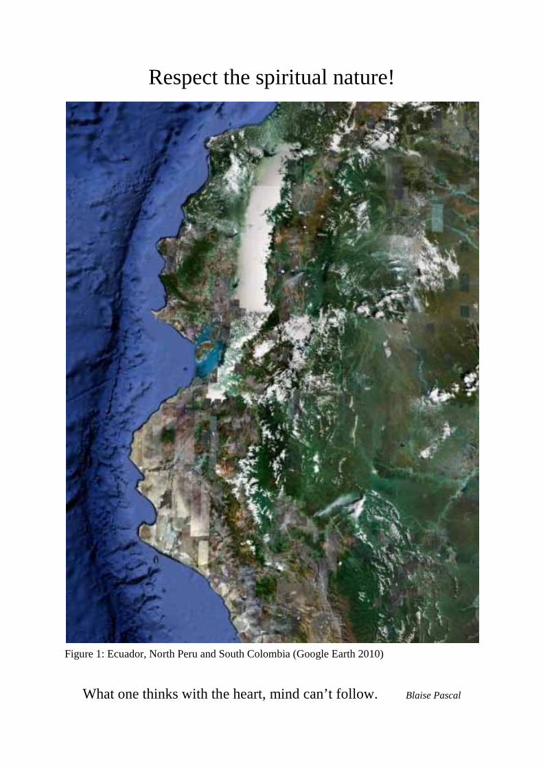
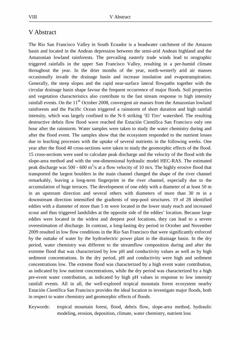
Figure 1: Ecuador, North Peru and South Colombia (Google Earth 2010)

What one thinks with the heart, mind can’t follow. Blaise Pascal

Table of contents � List of Figures .......................................................................................................................... I��� List of Tables ........................................................................................................................ V���� List of Abbreviations .......................................................................................................... VI��V Data DVD ......................................................................................................................... VII�V Abstract ............................................................................................................................. VIII�V� Zusammenfassung .............................................................................................................. IX 1 Introduction ............................................................................................................................ 1 2 Basics ..................................................................................................................................... 3

2.1 Definition of the Tropes and Climate Graph of Quito, Ecuador ...................................... 3�2.2 Plate Tectonics and Volcanoes in Ecuador ...................................................................... 4�2.3 Altitudinal Levels of the South American Andes ............................................................ 6�2.4 Deforestation and other Problems in Ecuador ................................................................ 10�2.5 Mangroves and Coral Reefs ........................................................................................... 16�2.6 Flood Climate ................................................................................................................. 20�2.7 Spatial and Temporal Scales of Hydroclimatic Activity ................................................ 26�2.8 Drainage Basin Morphometry ........................................................................................ 30�2.9 Runoff Generation .......................................................................................................... 39

3 State of the Art ..................................................................................................................... 45

3.1 Fluvial Geomorphology ................................................................................................. 45�3.2 Sediment Transport in the humid Tropics ...................................................................... 54�3.3 Flow Types ..................................................................................................................... 58�3.4 Geomorphic Impacts of Floods ...................................................................................... 65�3.5 Water Chemistry ............................................................................................................ 74�3.6 Runoff Generation in the humid Tropics ....................................................................... 76�3.7 Climate Change .............................................................................................................. 82�3.8 Paleoflood Hydrology .................................................................................................... 84

4 Methodology ........................................................................................................................ 91

4.1 Isotopes ........................................................................................................................... 91�4.2 Anions & Cations ........................................................................................................... 92�4.3 Water Samples ................................................................................................................ 93�4.4 Sediment ......................................................................................................................... 94�4.5 Cross-sectional Measurements ....................................................................................... 94�4.6 Slope-area Method ......................................................................................................... 95�4.6 Hydraulic Modeling with HEC-RAS ............................................................................. 97

5 Study Area .......................................................................................................................... 103

5.1 Geology ........................................................................................................................ 103�5.2 Landslides ..................................................................................................................... 108�5.3 Soils .............................................................................................................................. 112�5.4 Vegetation, Land Use, Biodiversity and Fire Dynamics .............................................. 117�5.5 Climate ......................................................................................................................... 127�5.6 El Niño ......................................................................................................................... 140�5.7 Flowpaths ..................................................................................................................... 143�5.8 Water Chemistry .......................................................................................................... 146�5.9 Nutrient Fluxes ............................................................................................................. 148�5.10 Impressions of the wider study area ........................................................................... 152

6 Results & Discussion ......................................................................................................... 155

6.1 Drainage Basin ............................................................................................................. 155

6.2 Climate ......................................................................................................................... 157

6.2.1 Landslides as indicator for maximum rainfall intensity ........................................ 157�6.2.2 Pre-Flood Conditions ............................................................................................ 158�6.2.3 Wind direction, wind velocity and rainfall intensity ............................................. 159�6.2.4 Air Temperature, Relative Humidity and Rainfall Intensity ................................. 160�6.2.5 Discussion ............................................................................................................. 161�6.2.6 Sea Surface Temperature....................................................................................... 162

6.3 Water Chemistry ......................................................................................................... 165

6.3.1 Conductivity and pH ............................................................................................. 165�6.3.2 Cations ................................................................................................................... 170�6.3.3 Anions ................................................................................................................... 178�6.3.4 Isotopes .................................................................................................................. 186�6.3.5 Sediment Concentration ........................................................................................ 188�6.3.6 Discussion ............................................................................................................. 191

6.4 Anthropogenic Influences ............................................................................................ 198

6.5 Hydraulics & discharge estimation .............................................................................. 204

6.5.1 Study Reach ........................................................................................................... 204�6.5.2 Cross-sectional Measurements .............................................................................. 205�6.5.3 Eddies .................................................................................................................... 207�6.5.4 Discussion ............................................................................................................. 210�6.5.5 Slope-area Method ................................................................................................ 213�6.5.6 HEC-RAS Modeling ............................................................................................. 214�6.5.7 Discussion ............................................................................................................. 215�6.5.8 Response Time ...................................................................................................... 216

6.6 Geomorphic Effects ...................................................................................................... 217

7 Conclusion .......................................................................................................................... 225 8 Acknowledgements ............................................................................................................ 229 9 Eidesstattliche Erklärung .................................................................................................... 231 10 Bibliography ..................................................................................................................... 233�

� List of Figures I

� List of Figures Figure 1: Ecuador, North Peru and South Colombia.................................................................... �Figure 2: Metric Climate Graph of Quito, Ecuador ................................................................... 3�Figure 3: Plates of the Earth ....................................................................................................... 4�Figure 4: Quilotoa Lagoon in Ecuador ....................................................................................... 5�Figure 5: Comparison between the Andes and the Alps ............................................................ 8�Figure 6: Deforestation in Morona Santiago on Shuar and Colonist land ............................... 12�Figure 7: Mangrove tree and kind of roots ............................................................................... 16�Figure 8: Geographic range of mangroves ............................................................................... 17�Figure 9: Extent of Shrimp farms in the Gulf of Guayaquil .................................................... 18�Figure 10: Position of the ITCZ in January and July. .............................................................. 21�Figure 11: Frequency of annual thunderstorms ........................................................................ 22�Figure 12: Zones of easterly wave and trade wind disturbance ............................................... 23�Figure 13: Flood climate regions of the world ......................................................................... 24�Figure 14: Meteorologic, climatologic and hydrologic space-time domain ............................ 26�Figure 15: Rainstorm event in the Walnut Gulch catchment ................................................... 28�Figure 16: Strahler ordering system of a drainage network and morphometric definitions..... 30�Figure 17: Drainage density and Thornthwaites precipitation effectiveness index ................. 31�Figure 18: Runoff hydrographs as a function of basin shape and bifurcation ratio ................. 32�Figure 19: Streamflow hydrograph resulting from a rainstorm ............................................... 33�Figure 20: Changes in lag time as a function of rainfall intensity ........................................... 34�Figure 21: Simulated Geomorphic Unit Hydrograph for a third-order basin........................... 35�Figure 22: Wave speed and travel time at flood discharges ..................................................... 36�Figure 23: Relationship between shear stress and velocity ...................................................... 38�Figure 24: Partial Area Model and Variable Source Area Model ............................................ 39�Figure 25: Relationship between infiltration volume and overland flow ................................. 40�Figure 26: Location of interrill, rill and gully erosion ............................................................. 41�Figure 27: Flow direction as controlled by soil anisotropy ...................................................... 42�Figure 28: Longitudinal profile of a river ................................................................................ 45�Figure 29: Meandering reach and areas of deposition and erosion .......................................... 46�Figure 30: Longitudinal profile of a riffle-pool sequence ........................................................ 46�Figure 31: Classification of bars .............................................................................................. 48�Figure 32: Bank erosion of a huge terrace in the Rio San Francisco Valley, Ecuador ............ 49�Figure 33: Relation of velocity and size of grains that can be eroded ..................................... 50�Figure 34: Profile of a rigid boundary channel ........................................................................ 51�Figure 35: Profile of a rigid boundary with floodplain vegetation .......................................... 51�Figure 36: Profile of changing cross-sections of a channel ..................................................... 52�Figure 37: Loose boundary textural and form drag resistance ................................................. 52�Figure 38: Flexible boundary resistance coefficient at low and high stage ............................. 53�Figure 39: Classification of suspensions based on shear strength & sediment concentration . 60�Figure 40: Channel widening due to the 1969 Hurricane Camille flood ................................. 66�Figure 41: Important factors controlling channel and floodplain response to floods .............. 71�Figure 42: Conceptual framework of runoff-generation mechanisms ..................................... 76�Figure 43: Ksat as function of soil depth ................................................................................... 78�Figure 44: Spectrum of hydrologic flowpaths in tropical rainforests ...................................... 79�Figure 45: Historical and paleoflood techniques for estimating paleoflood discharge ............ 86�Figure 46: Postbomb radiocarbon curve .................................................................................. 89�Figure 47: Conservation of energy for gradually varied flow .................................................. 98�Figure 48: Specific energy curve ............................................................................................. 99�

II � List of Figures

Figure 49: Hydraulic modeling .............................................................................................. 100�Figure 50: Topography and geology of the ‘Cordillera Real’ ................................................ 103�Figure 51: Upper tree line and lowest glacial stands within the west-Andes ........................ 104�Figure 52: Study area below the ‘El Tiro’ watershed ............................................................ 104�Figure 53: ‘El Tiro’ watershed in the upper Rio San Francisco Valley ................................. 105�Figure 54: Extension of the Páramo ....................................................................................... 106�Figure 55: Orographic map and river systems in Ecuador ..................................................... 107�Figure 56: Classification of rapid mass movements .............................................................. 108�Figure 57: Distribution of landslides on RBSF terrain .......................................................... 109�Figure 58: Landslides of a section of Quebrada Milagro ....................................................... 110�Figure 59: Successional stages on landslides ......................................................................... 111�Figure 60: Relationship between altitude and C/N ratio in organic layers. ........................... 112�Figure 61: Typical Cambisol after dye tracer experiment in the forested study area ............ 113�Figure 62: Relationship between calcium and pH and magnesium and pH in O horizons .... 115�Figure 63: Cation-exchange capacity, base saturation and C concentrations of soils ............ 115�Figure 64: Potential natural vegetation of the Cordillera Real and land-use pattern ............. 117�Figure 65: Profile diagram of Forest Type 1 at the RBSF (1960 m) ..................................... 119�Figure 66: Profile diagram of Forest Type 2 at the RBSF (2050 m) ..................................... 119�Figure 67: Profile diagram of Forest Type 3 at the RBSF (2210 m) ..................................... 120�Figure 68: Profile diagram of Forest Type 4 at the RBSF (2450 m) ..................................... 120�Figure 69: Profile diagram of Forest Type 5 at the RBSF (3000 m) ..................................... 121�Figure 70: Pollen percentage diagram and spore taxa from the RBSF - T2/250 ................... 123�Figure 71: Pollen percentage diagram and spore taxa from the Refugio ............................... 124�Figure 72: Pollen percentage diagram of pollen and spore taxa from El Tiro Pass ............... 125�Figure 73: Average air temperature along the altitudinal transect ......................................... 127�Figure 74: Average hourly irradiance along the altitudinal transect ...................................... 128�Figure 75: Cloud frequency along the western- and eastern Andean mountain range........... 129�Figure 76: Average wind velocity along the altitudinal transect ........................................... 130�Figure 77: Frequency of wind direction, rainfall and rain rate at the Páramo MS ................. 131�Figure 78: Average monthly rainfall along the altitudinal transect........................................ 133�Figure 79: Average monthly fog water intake along the altitudinal gradient ........................ 133�Figure 80: Average relative humidity along the altitudinal gradient ..................................... 136�Figure 81: Altitudinal gradients of pH, conductivity and ion concentrations in rain water ... 137�Figure 82: Altitudinal gradients of pH, conductivity and ion concentrations in fog water .... 137�Figure 83: Time series of monthly mean ion concentrations in rain and fog water .............. 138�Figure 84: Time series of fire frequency ................................................................................ 139�Figure 85: Ten-day daily backward trajectories ..................................................................... 139�Figure 86: Wind and rainfall in Ecuador during El Niño and normal conditions .................. 140�Figure 87: Cloud motion winds in the central Niño area of Ecuador and Northern Peru ...... 141�Figure 88: Average MCSST ................................................................................................... 142�Figure 89: Mean �18O values in rainfall and streamwater ...................................................... 144�Figure 90: Course of soil water content during a rainstorm event ......................................... 145�Figure 91: Estación Científica San Francisco, Pastos and RBSF study area ......................... 152�Figure 92: Cajanuma at 3400 m and Bombuscaro at 1000 m ................................................ 152�Figure 93: Tarabita during the mudflow phase, steps to overcome the steep slopes ............. 152�Figure 94: Rio San Francisco Valley, above the tara bita rock face ...................................... 153�Figure 95: Bacteria and algae in the river bed in the dry period 2009 ................................... 153�Figure 96: Rio San Francisco, variable source area ............................................................... 153�Figure 97: Antennas, upper Rio San Francisco headwaters ................................................... 153�Figure 98: Wider study area in South Ecuador showing the ‘Cordillera Real’ ...................... 155�Figure 99: Drainage network system of the study area .......................................................... 156�

� List of Figures III

Figure 100: RBSF study area ................................................................................................. 156�Figure 101: Landslides and incised Jipiro on the western slope of the ‘El Tiro watershed’ . 157�Figure 102: rainfall intensity, air temperature and relative humidity before the flood .......... 158�Figure 103: Wind direction and wind velocity at the El Tiro watershed ............................... 159�Figure 104: Air temperature, relative humidity, precipitation intensity at El Tiro watershed 160�Figure 105: Niño 4, Niño 3, Niño 1+2 and Costero ............................................................... 162�Figure 106: Sea Surface Temperature anomalies for Costero area ........................................ 163�Figure 107: Weekly Sea Surface Temperature anomalies relative to 1971-2000 .................. 164�Figure 108: Conductivity and pH in the flood phase ............................................................. 165�Figure 109: Conductivity and pH in the recovery phase ........................................................ 166�Figure 110: Conductivity and pH in the post-flood phase ..................................................... 167�Figure 111: Conductivity and pH in the dry period 2009 ...................................................... 168�Figure 112: Box Plots of conductivity in the different phases ............................................... 169�Figure 113: Box Plots of pH in the different phases .............................................................. 169�Figure 114: Concentrations of magnesium and calcium in the flood phase .......................... 170�Figure 115: Concentrations of magnesium and calcium in the recovery phase ..................... 171�Figure 116: Concentrations of magnesium and calcium in the post-flood phase .................. 172�Figure 117: Box Plots of magnesium concentrations in the different phases. ....................... 173�Figure 118: Box Plots of calcium concentrations in the different phases .............................. 173�Figure 119: Concentrations of sodium and potassium in the flood phase ............................. 174�Figure 120: Concentrations of sodium and potassium in the recovery phase ........................ 175�Figure 121: Concentrations of sodium and potassium in the post-flood phase...................... 176�Figure 122: Box Plots of sodium concentrations in the different phases ............................... 177�Figure 123: Box Plots of potassium concentrations in the different phases .......................... 177�Figure 124: Concentrations of nitrate and phosphate in the flood phase ............................... 178�Figure 125: Concentrations of nitrate and phosphate in the recovery phase.......................... 179�Figure 126: Concentrations of nitrate and phosphate in the post-flood phase ....................... 180�Figure 127: Box Plots of nitrate concentrations in the different phases ................................ 181�Figure 128: Box Plots of phosphate concentrations in the different phases .......................... 181�Figure 129: Concentrations of sulphate and chloride in the flood phase ............................... 182�Figure 130: Concentrations of sulphate and chloride in the recovery phase.......................... 183�Figure 131: Concentrations of sulphate and chloride in the post-flood phase ....................... 184�Figure 132: Box Plots of sulphate concentrations in the different phases ............................. 185�Figure 133: Box Plots of chloride concentrations in the different phases ............................. 185�Figure 134: Isotope contents of �18O and �2H in the flood phase .......................................... 186�Figure 135: Isotope contents of �18O and �2H in the recovery phase..................................... 186�Figure 136: Isotope contents of �18O and �2H in the post-flood phase .................................. 187�Figure 137: Box Plots of �18O and �2H contents in the different phases ............................... 187�Figure 138: Sediment concentrations in the flood phase ....................................................... 188�Figure 139: Sediment concentrations in the recovery phase .................................................. 188�Figure 140: Sediment concentrations in the post-flood phase ............................................... 189�Figure 141: Sediment concentrations in the dry period 2009 ................................................ 190�Figure 142: Box Plots of sediment concentrations in the different phases ............................ 190�Figure 143: Compuerta after the extreme flood ..................................................................... 198�Figure 144: Flow conditions of the ‘Camino Canal’ in the dry period 2009 ......................... 198�Figure 145: Extreme low flow conditions in the Rio San Francisco ..................................... 199�Figure 146: ‘Planta’ and ‘Quebrada Milagro’, surplus water of the ‘Camino Canal’ ........... 200�Figure 147: Nightly fire at the ‘Planta’ in the dry period ....................................................... 201�Figure 148: Road from Loja to Zamora at the ‘El Tiro’ watershed ....................................... 201�Figure 149: Gullies extending from the road to the streams .................................................. 202�Figure 150: Flood protection structure built after the extreme flood ..................................... 202�

IV � List of Figures

Figure 151: Peak discharge influencing bridge through backwater effects ........................... 203�Figure 152: Landslides on the road from Loja to Zamora ..................................................... 203�Figure 153: The three sub-reaches of the whole study reach ................................................. 204�Figure 154: Schematic overview over the three sub-reaches ................................................. 204�Figure 155: Average mean flow depth of the cross-sections ................................................. 205�Figure 156: Average maximum flow depth of the cross-sections .......................................... 205�Figure 157: Average channel width of the cross-sections ...................................................... 206�Figure 158: Average cross-sectional area of the cross-sections ............................................. 206�Figure 159: Number of eddies and diameters in the whole reach and in the tara bita reach.. 207�Figure 160: Average distance of eddies in the whole reach and in the tara bita reach .......... 207�Figure 161: Super-elevation and bed slope of different hydraulic features and locations ..... 208�Figure 162: Water surface inclination in the bend after the straight run of the zig zag reach 209�Figure 163: Super-elevation of the water surface at the tara bita rock face ........................... 210�Figure 164: Eddies, terraces, landslides and other channel features of all cross-sections ..... 211�Figure 165: Lower tara bita reach before and after the flood ................................................. 212�Figure 166: Hillslope, high water mark, water surface inclination and eddies ...................... 212�Figure 167: Velocity calculated with Manning’s and Chezy’s equation ............................... 213�Figure 168: Discharge calculated with Manning’s and Chezy’s equation ............................. 213�Figure 169: Modeled water level surfaces with HEC-RAS 4.0 ............................................. 214�Figure 170: Precipitation intensity at ‘El Tiro’ and response time of the Rio San Francisco 216�Figure 171: Geomorphic effects in the rock face reach ......................................................... 218�Figure 172: Rock face reach one year after the flood ............................................................ 219�Figure 173: Large boulders that have been transported during the flood .............................. 219�Figure 174: Tara bita rock face before (left) and after (right) the flood ................................ 220�Figure 175: High water marks on the tara bita rock face ....................................................... 220�Figure 176: Circular boulder deposition of a large eddy in the tara bita rock face ................ 221�Figure 177: Potholes occurring in couples or series .............................................................. 221�Figure 178: Rock spurs in steep bends ................................................................................... 222�Figure 179: Rock face of the rock face reach ......................................................................... 222�Figure 180: Catfish astroblepus ............................................................................................. 223�Figure 181: Largest eddy in the study reach .......................................................................... 224�Figure 182: Terrace with high flow channel, 6 m, 14 m and 36 m stage of the 50 m eddy ... 224

�� List of Tables V

�� List of Tables Table 1: Deforestation of Colonist and Shuar communities in Morona Santiago, Ecuador .... 12�Table 2: Classification of flows with high sediment concentrations ....................................... 58�Table 3: Geomorphic and sedimentologic characteristics of water and sediment flows ......... 59�Table 4: Geomorphic effects of major floods .......................................................................... 69�Table 5: Chemical composition of river water of the world .................................................... 74�Table 6: Typical Slackwater Deposit radiocarbon dating materials ........................................ 88�Table 7: Manning’s roughness coefficient values .................................................................... 96�Table 8: Mean element concentrations in the O horizons in South Ecuador ......................... 113�Table 9: Water surplus due to horizontal rain and cloud or fog water deposition ................. 134�Table 10: Characteristic parameters of the study area and other tropical ecosystems ........... 151�

VI ��� List of Abbreviations

��� List of Abbreviations ASCE American Society of Civil Engineers BAC Boletín de Alerta Climático C-CONDEM Corporación Coordianadora Nacional Para La Defensa Del Ecosistma Manglar CLIRSEN Centro De Levantamientos Integrados De Recursos Naturales Por Sensores

Remotos CONAIE Confederación de Nacionalidades Indígenas del Ecuador CPPS Comisión Permanente del Pacífico Sur ECSF Estación Científica San Francisco ERFEN Estudio Regional del Fenómeno El Niño FAO Food and Agriculture Organization FC Fog Collector ITCZ Inter-tropical Convergence Zone GTZ Gesellschaft für Technische Zusammenarbeit GUH Geomorphic Unit Hydrograph HEC-RAS Hydrologic Engineering Center - River Analysis System INOCAR Oceanographic Institute of the Navy of Ecuador IPCC Intergovernmental Panel on Climate Change MS Meteorologic Station NCEP National Centers for Environmental Prediction NOAA National Oceanic and Atmospheric Administration NWS National Weather Service RBSF Reserva Biologíca San Francisco RT Rainfall Totaliser UNEP United Nations Environmental Programme WMO World Meteorologic Organization

H+ hydrogenium Na+ sodium K+ potassium Mg2+ magnesium Ca2+ calcium Cl- chloride SO4

2- sulphate NO3

- nitrate PO4

3- phosphate 18O oxygen-18 2H deuterium pH negative logarithm base 10 of [H+]

DOM dissolved organic matter DOC dissolved organic carbon DON dissolved organic nitrogen DOP dissolved organic phosphor DOS dissolved organic sulphur Fe iron S sulphur P phosphorus N nitrogen NH4

+ methane CO2 carbon dioxide

�V Data DVD VII

�V Data DVD The included DVD contains:

- Data Documentation

- Pictures of the Flood:

- before the flood

- during the flood

- after the flood

- one year after the flood

- Videos of the Flood

- Newspaper articles of the flood published in ‘La Hora’, Loja, in Spanish

- Informations of anthropogenic influences on flood generation, in Spanish

- Pictures of erosion, scour and deposition from the ‘Compuerta’ to the ‘Planta’

- Pictures of the eddies

- Pictures of the succession stages on the two major terraces in the study reach

- Pictures of the biota

- Pictures of the mangroves on Jambeli, Gulf of Guayaquil, Ecuador

- Pictures of gold mining in Nambija, Ecuador

- Report on gold mining in developing countries, in German

VIII V Abstract

V Abstract

The Rio San Francisco Valley in South Ecuador is a headwater catchment of the Amazon basin and located in the Andean depression between the semi-arid Andean highland and the Amazonian lowland rainforests. The prevailing easterly trade winds lead to orographic triggered rainfalls in the upper San Francisco Valley, resulting in a per-humid climate throughout the year. In the drier months of the year, north-westerly arid air masses occasionally invade the drainage basin and increase insolation and evapotranspiration. Generally, the steep slopes and the rapid near-surface lateral flowpaths together with the circular drainage basin shape favour the frequent occurrence of major floods. Soil properties and vegetation characteristics also contribute to the fast stream response to high intensity rainfall events. On the 11th October 2008, convergent air masses from the Amazonian lowland rainforests and the Pacific Ocean triggered a rainstorm of short duration and high rainfall intensity, which was largely confined to the N-S striking ‘El Tiro’ watershed. The resulting destructive debris flow flood wave reached the Estación Científica San Francisco only one hour after the rainstorm. Water samples were taken to study the water chemistry during and after the flood event. The samples show that the ecosystem responded to the nutrient losses due to leaching processes with the uptake of several nutrients in the following weeks. One year after the flood 40 cross-sections were taken to study the geomorphic effects of the flood. 15 cross-sections were used to calculate peak discharge and the velocity of the flood with the slope-area method and with the one-dimensional hydraulic model HEC-RAS. The estimated peak discharge was 500 - 600 m3/s at a flow velocity of 10 m/s. The highly erosive flood that transported the largest boulders in the main channel changed the shape of the river channel remarkably, leaving a long-term fingerprint in the river channel, especially due to the accumulation of huge terraces. The development of one eddy with a diameter of at least 50 m in an upstream direction and several others with diameters of more than 30 m in a downstream direction intensified the gradients of step-pool structures. 19 of 28 identified eddies with a diameter of more than 5 m were located in the lower study reach and increased scour and thus triggered landslides at the opposite side of the eddies’ location. Because large eddies were located in the widest and deepest pool locations, they can lead to a severe overestimation of discharge. In contrast, a long-lasting dry period in October and November 2009 resulted in low flow conditions in the Rio San Francisco that were significantly enforced by the outtake of water by the hydroelectric power plant in the drainage basin. In the dry period, water chemistry was different to the streamflow composition during and after the extreme flood that was characterized by low pH and conductivity values as well as by high sediment concentrations. In the dry period, pH and conductivity were high and sediment concentrations low. The extreme flood was characterized by a high event water contribution, as indicated by low nutrient concentrations, while the dry period was characterized by a high pre-event water contribution, as indicated by high pH values in response to low intensity rainfall events. All in all, the well-explored tropical mountain forest ecosystem nearby Estación Científica San Francisco provides the ideal location to investigate major floods, both in respect to water chemistry and geomorphic effects of floods.

Keywords: tropical mountain forest, flood, debris flow, slope-area method, hydraulic modeling, erosion, deposition, climate, water chemistry, nutrient loss

V� Zusammenfassung IX

V� Zusammenfassung

Das Rio San Francisco Tal ist ein Einzugsgebiet des Amazonas und befindet sich in der Anden-Depression von Süd-Ecuador zwischen dem semi-ariden Hochland und dem immer feuchten Tieflandregenwald. Der östliche Passatwind dominiert das immer feuchte Klima insbesondere durch orographischen Niederschlag an der östlichen Andenkette. In den trockeneren Monaten des Jahres dringen gelegentlich trockene nord-west Winde von der Küste in das Rio San Francisco Tal ein und erhöhen die Sonneneinstrahlung und damit auch die Verdunstung von Oberflächen und Pflanzen durch trockene Fallwinde. Die Entstehung großer Hochwasser im Untersuchungsgebiet wird durch die steilen Hänge, durch die schnellen oberflächennahen Fließwege und die runde Form des Einzugsgebietes begünstigt. Die schnelle Reaktion des Abflusses wird zudem von Bodeneigenschaften und der höhenbedingten Vegetationsverteilung beeinflusst. Die klimatische Situation am 11. Oktober 2008 führte zu konvergierenden Luftmassen aus Amazonien und vom Pazifischen Ozean. Die kollidierenden und aufsteigenden Luftmassen führten zu einem heftigen kurzen und räumlich begrenzten Regenschauer über der Wasserscheide des ‘El Tiro’ Kammes. Die durch Niederschlag und Hangrutsche erzeugte zerstörerische Geröllflutwelle erreichte die Forschungsstation Estación Científica San Francisco nach nur einer Stunde. Während und nach dem Hochwasser wurden Wasserproben genommen um Einblicke in die Wasserchemie zu gewinnen. Das Ökosystem des tropischen Bergnebelregenwaldes reagierte auf den Nährstoffverlust durch Auswaschungsprozesse mit dem Rückhalt einiger wichtiger Pflanzennährstoffe in den folgenden Wochen. Im darauffolgenden Jahr wurden 40 Querschnittprofile vermessen um die geomorphologischen Auswirkungen des Hochwassers zu dokumentieren. Um den Abfluss und die Fließgeschwindigkeit des Hochwassers mit der Gradientenmethode und dem ein-dimensionalen hydraulischen Model HEC-RAS zu bestimmen, wurden 15 Querschnittprofile verwendet. Der geschätzte Abfluss betrug 500 - 600 m3/s bei einer Fließgeschwindigkeit von 10 m/s. Die zerstörerische Flutwelle transportierte die größten Felsbrocken im Flussbett und führte zur Ablagerung mächtiger Terrassen. Wasserwirbel, die sich bevorzugt in den tiefsten und weitesten Orten des Flussbettes entwickelten, verstärkten das lokale Gefälle zwischen Stufen und zugehörigen Becken. 19 von 28 Wasserwirbel bildeten sich im unteren Bereich des 800 m langen untersuchten Flussabschnitts. Die Wasserwirbel beeinflussten die Hydraulik und führten zu erhöhter Erosion an den gegenüberliegenden Hängen. Die Trockenperiode 2009 führte zu einem sehr geringen Abfluss im Rio San Francisco, der durch die Wasserentnahme des Wasserkraftwerkes ‘Planta’ entscheidend verschärft wurde. Die Wasserzusammensetzung der Trockenperiode unterschied sich entscheidend von der Hochwasserperiode, die durch niedrige pH und Leitfähigkeitswerte, sowie durch hohe Sedimentkonzentrationen gekennzeichnet war. Die Trockenperiode wurde von hohen pH und Leitfähigkeitswerten und geringen Sedimentkonzentrationen bestimmt und führte dem Hauptfluss bevorzugt Vorereigniswasser zu, während die Hochwasserperiode durch Zufluss von Ereigniswasser dominiert wurde. Der gut erforschte tropische Bergnebelregenwald Süd-Ecuadors und die Estación Científica San Francisco bieten ideale Voraussetzungen für Hochwasserstudien.

Schlüsselwörter: tropischer Bergnebelregenwald, Hochwasser, Erosion, Deposition, Gradientenmethode, hydraulische Modellierung, Nährstoffverlust

X V� Zusammenfassung

1 Introduction 1

1 Introduction

There is a close relationship between the source of all life and natural rivers. Streams provide drinking water, food, water for irrigation, land drainage, waste disposal, a source of power and a transport medium to the ocean. Because of the widespread use of flat and fertile alluvial land for agriculture and construction, floods frequently affect people and require investigation (Allan & Castillo 2007). Rivers are dynamic components of the landscape. As streamflow contains solid and dissolved substances, energy, mass and nutrients are transported from one location in the landscape to another. High intensity rainfalls that result in floods can produce rapid hydrologic and geomorphic responses that may affect large areas. Geomorphic transformation takes place within a short time and depends on the size of the river as well as on terrain and climatic features (Baker et al. 1988). Streams may shift course and change size, sediment loads may fluctuate, floods scour and deposit, banks collapse, huge boulders may move and thick layers of sediment may be deposited or eroded. Secondary flows, such as eddies can have a significant influence on hydraulic features during major floods and thus on erosion and deposition of organic and inorganic matter (Gordon et al. 2004). Studies on the geomorphic effects of floods are an efficient way to understand past, present and future earth surface processes. Major rainfall events and extreme floods often occur in inaccessible locations like in steep headwater catchments where natural metamorphosis of geomorphic flood effects, such as sedimentary features and high-water marks may be eroded or changed by following floods within a short time (Baker et al. 1988).

The hydrology and geomorphology of a river and its valley are closely linked to the shape of the river channel (Allan & Castillo 2007). For that reason, geomorphic effects of force, resistance, erosion, transportation and deposition can be best analysed in river channels. Geomorphologic and hydrologic studies after rare flood events provide insight into drainage basin processes (Baker et al. 1988). Rainfall, fog and snow that fall within a drainage basin reach the stream via numerous flowpaths. Overland flow and near-subsurface stormflow, following a rainstorm, reach the streams quickly and can produce flashy floods. In contrast, groundwater reaches the stream delayed, due to the longer and slower flowpaths through the soil matrix. Subsurface flow is more likely to take on the chemical signature of the underlying geology by dissolving more minerals. In natural ecosystems, drainage basin characteristics, such as geology, topography and vegetation, as well as climatic features influence these flowpaths (Allan & Castillo 2007).

Studies of the ecology and hydrology of streams depend on information on water chemistry and on the size and distribution of organic and inorganic particles, whether in motion or forming part of the river beds, banks and slopes. Streamwater chemistry reflects the nature of actual ongoing processes within a drainage basin at a certain time and place. Changes in the chemical composition thus contain information about the origin and the flowpaths of the constituents. In this context, the influence of a flood on the nutrient cycle of a ecosystem can be studied both in respect of the nutrient losses due to leaching processes and mass movement events, as well as in respect to the response of the catchment to flood associated features (Gordon et al. 2004).

2 1 Introduction

In October 2008 I made a lab on the Estación Científica San Francisco in South Ecuador in the tropical mountain forest ecosystem nearby the Reserve Podocarpus. At the end of my training, a major flood event occurred in the upper Rio San Francisco Valley. I decided to sample streamwater for one month to study the effects of the flood on the ecosystem. I decided to return to Ecuador to document the geomorphic effects of the flood in the Rio San Francisco headwater catchment of the mighty Amazon. When I arrived at the scientific station the driest period in Ecuador since 45 years affected the ecosystem. Therefore, I again took water samples for a complete month while I made the planned cross-sectional measurements.

The objective of this study is to determine major climatic and geomorphic factors that influenced and favoured the extreme flood of 11th October 2008 in the Rio San Francisco Valley in South Ecuador. As water samples were taken for the complete month after the flood event and analysed for anions, cations, sediment concentrations and isotopes, the major focus will be on the response of the ecosystem to the nutrient losses caused by the rainstorm, as well as on the general response of the drainage basin to rainfall events. The chemical hydrographs should reflect that different flowpaths are involved in runoff generation. In respect of geomorphology, the aim of the study will be on the description of the hydraulics and associated erosional and depositional features. In respect of hydrology, the focus will be on the determination of peak discharge and flow velocity through the slope-area method and the one-dimensional hydraulic model HEC-RAS. Another aim is to study the characteristics of large eddies. For these objectives, 40 cross-sections were measured in a reach of 800 m in length to analyse the impact of large eddies on the channel shape and on associated erosional and depositional features. The main focus, regarding climatic processes will be on meteorologic and climatologic configurations that triggered the rainstorm at the ‘El Tiro’ watershed in the ‘Cordillera Real’, the east Andean mountain range.

2 Basics 3

2 Basics 2.1 Definition of the Tropes and Climate Graph of Quito, Ecuador

The tropes can be limited in three different ways: through the astronomic borderlines of the northern tropic of Cancer and the southern tropic of Capricorn. The space in between the tropics from 23.5° N to 23.5° S forms a belt of more than 5000 km width (Blüthgen 1966); through the determination of frost-free zones throughout the year. This kind of boundary is generally less precise, because in tropical highlands frost can occur throughout the year but for tropical lowlands, it is a good criterion; through the definition of the tropes by the regions, where the average daily variations of temperature are higher than the average annual variations of temperature (Blüthgen & Weischet 1980).

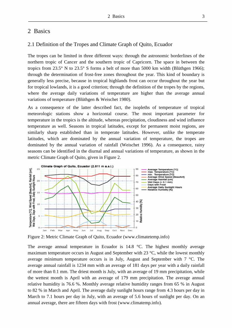
As a consequence of the latter described fact, the isopleths of temperature of tropical meteorologic stations show a horizontal course. The most important parameter for temperature in the tropics is the altitude, whereas precipitation, cloudiness and wind influence temperature as well. Seasons in tropical latitudes, except for permanent moist regions, are similarly sharp established than in temperate latitudes. However, unlike the temperate latitudes, which are dominated by the annual variation of temperature, the tropes are dominated by the annual variation of rainfall (Weischet 1996). As a consequence, rainy seasons can be identified in the diurnal and annual variations of temperature, as shown in the metric Climate Graph of Quito, given in Figure 2.

Figure 2: Metric Climate Graph of Quito, Ecuador (www.climatetemp.info)

The average annual temperature in Ecuador is 14.8 °C. The highest monthly average maximum temperature occurs in August and September with 23 °C, while the lowest monthly average minimum temperature occurs is in July, August and September with 7 °C. The average annual rainfall is 1234 mm with an average of 181 days per year with a daily rainfall of more than 0.1 mm. The driest month is July, with an average of 19 mm precipitation, while the wettest month is April with an average of 179 mm precipitation. The average annual relative humidity is 76.6 %. Monthly average relative humidity ranges from 65 % in August to 82 % in March and April. The average daily sunlight hours range from 4.3 hours per day in March to 7.1 hours per day in July, with an average of 5.6 hours of sunlight per day. On an annual average, there are fifteen days with frost (www.climatemp.info).

4 2 Basics

2.2 Plate Tectonics and Volcanoes in Ecuador

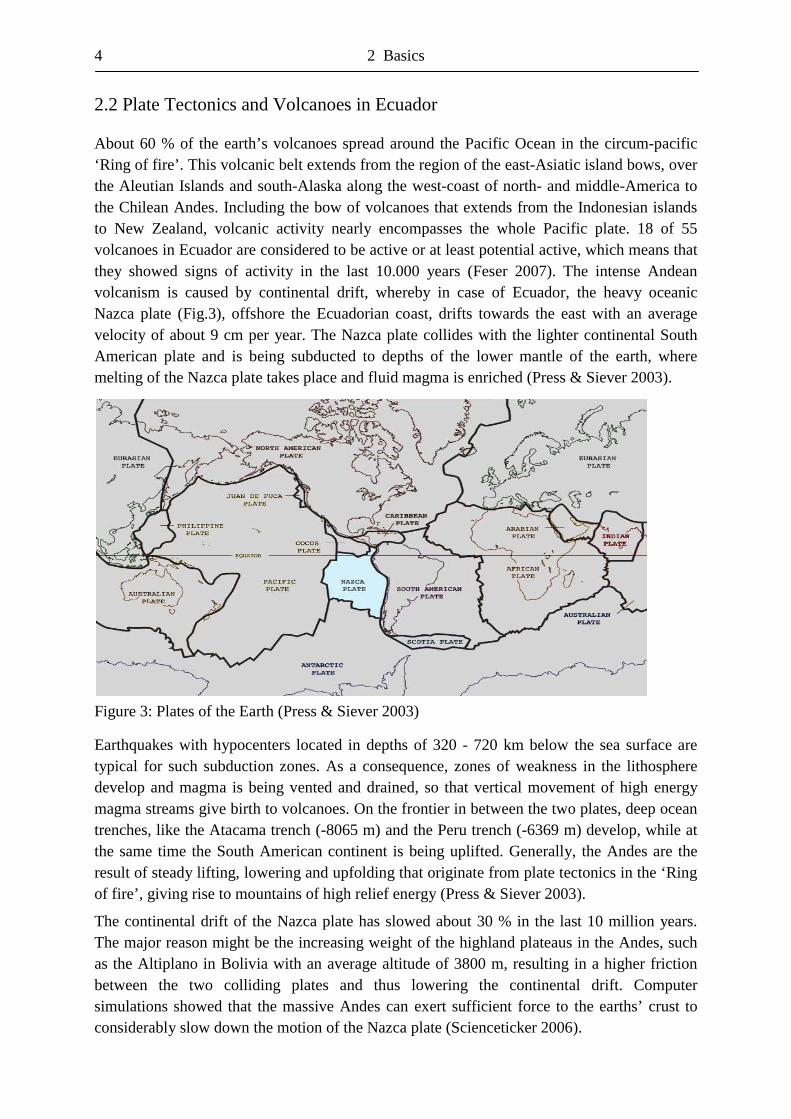
About 60 % of the earth’s volcanoes spread around the Pacific Ocean in the circum-pacific ‘Ring of fire’. This volcanic belt extends from the region of the east-Asiatic island bows, over the Aleutian Islands and south-Alaska along the west-coast of north- and middle-America to the Chilean Andes. Including the bow of volcanoes that extends from the Indonesian islands to New Zealand, volcanic activity nearly encompasses the whole Pacific plate. 18 of 55 volcanoes in Ecuador are considered to be active or at least potential active, which means that they showed signs of activity in the last 10.000 years (Feser 2007). The intense Andean volcanism is caused by continental drift, whereby in case of Ecuador, the heavy oceanic Nazca plate (Fig.3), offshore the Ecuadorian coast, drifts towards the east with an average velocity of about 9 cm per year. The Nazca plate collides with the lighter continental South American plate and is being subducted to depths of the lower mantle of the earth, where melting of the Nazca plate takes place and fluid magma is enriched (Press & Siever 2003).

Figure 3: Plates of the Earth (Press & Siever 2003)

Earthquakes with hypocenters located in depths of 320 - 720 km below the sea surface are typical for such subduction zones. As a consequence, zones of weakness in the lithosphere develop and magma is being vented and drained, so that vertical movement of high energy magma streams give birth to volcanoes. On the frontier in between the two plates, deep ocean trenches, like the Atacama trench (-8065 m) and the Peru trench (-6369 m) develop, while at the same time the South American continent is being uplifted. Generally, the Andes are the result of steady lifting, lowering and upfolding that originate from plate tectonics in the ‘Ring of fire’, giving rise to mountains of high relief energy (Press & Siever 2003).

The continental drift of the Nazca plate has slowed about 30 % in the last 10 million years. The major reason might be the increasing weight of the highland plateaus in the Andes, such as the Altiplano in Bolivia with an average altitude of 3800 m, resulting in a higher friction between the two colliding plates and thus lowering the continental drift. Computer simulations showed that the massive Andes can exert sufficient force to the earths’ crust to considerably slow down the motion of the Nazca plate (Scienceticker 2006).

2 Basics 5

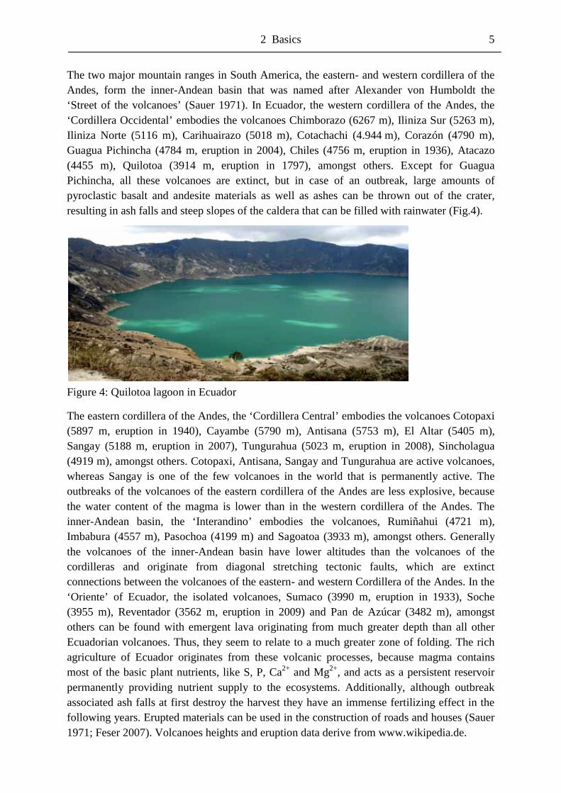
The two major mountain ranges in South America, the eastern- and western cordillera of the Andes, form the inner-Andean basin that was named after Alexander von Humboldt the ‘Street of the volcanoes’ (Sauer 1971). In Ecuador, the western cordillera of the Andes, the ‘Cordillera Occidental’ embodies the volcanoes Chimborazo (6267 m), Iliniza Sur (5263 m), Iliniza Norte (5116 m), Carihuairazo (5018 m), Cotachachi (4.944 m), Corazón (4790 m), Guagua Pichincha (4784 m, eruption in 2004), Chiles (4756 m, eruption in 1936), Atacazo (4455 m), Quilotoa (3914 m, eruption in 1797), amongst others. Except for Guagua Pichincha, all these volcanoes are extinct, but in case of an outbreak, large amounts of pyroclastic basalt and andesite materials as well as ashes can be thrown out of the crater, resulting in ash falls and steep slopes of the caldera that can be filled with rainwater (Fig.4).

Figure 4: Quilotoa lagoon in Ecuador

The eastern cordillera of the Andes, the ‘Cordillera Central’ embodies the volcanoes Cotopaxi (5897 m, eruption in 1940), Cayambe (5790 m), Antisana (5753 m), El Altar (5405 m), Sangay (5188 m, eruption in 2007), Tungurahua (5023 m, eruption in 2008), Sincholagua (4919 m), amongst others. Cotopaxi, Antisana, Sangay and Tungurahua are active volcanoes, whereas Sangay is one of the few volcanoes in the world that is permanently active. The outbreaks of the volcanoes of the eastern cordillera of the Andes are less explosive, because the water content of the magma is lower than in the western cordillera of the Andes. The inner-Andean basin, the ‘Interandino’ embodies the volcanoes, Rumiñahui (4721 m), Imbabura (4557 m), Pasochoa (4199 m) and Sagoatoa (3933 m), amongst others. Generally the volcanoes of the inner-Andean basin have lower altitudes than the volcanoes of the cordilleras and originate from diagonal stretching tectonic faults, which are extinct connections between the volcanoes of the eastern- and western Cordillera of the Andes. In the ‘Oriente’ of Ecuador, the isolated volcanoes, Sumaco (3990 m, eruption in 1933), Soche (3955 m), Reventador (3562 m, eruption in 2009) and Pan de Azúcar (3482 m), amongst others can be found with emergent lava originating from much greater depth than all other Ecuadorian volcanoes. Thus, they seem to relate to a much greater zone of folding. The rich agriculture of Ecuador originates from these volcanic processes, because magma contains most of the basic plant nutrients, like S, P, Ca2+ and Mg2+, and acts as a persistent reservoir permanently providing nutrient supply to the ecosystems. Additionally, although outbreak associated ash falls at first destroy the harvest they have an immense fertilizing effect in the following years. Erupted materials can be used in the construction of roads and houses (Sauer 1971; Feser 2007). Volcanoes heights and eruption data derive from www.wikipedia.de.

6 2 Basics

2.3 Altitudinal Levels of the South American Andes

One of the most important factors for the development of the characteristics of different altitudinal steps in the tropical Andes is the decrease of temperature with increasing altitude. The average annual temperature decreases about 0.5 - 0.6 K per 100 m. In reality every region is shaped by its individual characteristic environment, so that these values vary, depending on season, geographical latitude, regional differences and special features. Another important factor is the individual vertical distribution of precipitation in the Andes. Unlike in humid mountain regions of the moderate latitudes, such as the Alps in Europe, where the amount of rainfall relative constantly increases with increasing altitude, in the tropical Andes there is an altitudinal belt of maximum precipitation established in an altitude between 900 - 1500 m. Immediately above this boundary, the 1st level of water vapour condensation is located, with a subsequent 2nd level of water vapour condensation above 2700 m (Lauer & Erlenbach 1987).

The altitudinal steps of the tropical Andes were named according to their characteristic air temperature. Following descriptions have primary been developed by Alexander von Humboldt and encompass mountain ecosystems of the tropical Andes of South America, in which the whole complexity of climate, characteristics of the vegetation, agricultural use, and the shaping of the cultural landscape flow in (Lauer & Erlenbach 1987).

In the 1st altitudinal level, the hot land or ‘tierra caliente’, reaching up to 1100 m, the average annual temperature is about 19 - 27 °C. The region is hot and widely characterized by tropical evergreen lowland rainforests, e.g. in the Amazon basin, including the lower east-Andean slopes of the ‘Cordillera Real’, where the Ecuadorian ‘Oriente’ and Zamora is located.

In the 2nd altitudinal level, the temperate land or ‘tierra templada’, reaching up to 2500 m, the average annual temperature values about 12 - 15 °C at the upper limits. The region is moderate and characterized by tropical mountain forests, e.g. the Rio San Francisco Valley in the study area, located between ‘El Oriente’ and the Andean highland, e.g ECSF and Loja.

In the 3rd altitudinal level, the cold land or ‘tierra fría’, reaching up to 3800 m, the average annual temperature values about 5 - 8 °C. The region is cold and characterized by very good conditions to grow European field crops. Below the lower boundary of this altitudinal level, the absolute frost line is located, e.g. ‘El Tiro’ watershed on the crest of the ‘Cordillera Real’ at 2750 m up to the highest mountain ‘Antennas’ in the study area at 3200 m.

In the 4th altitudinal level, the frost land or ‘tierra helada’, reaching up to 4800 m as far as the forelands of the glaciers, the average annual temperature values about 0 - 6 °C. The region is icy and characterized by steppe, e.g. Ecuadorian volcanoes like Tungurahua and Rumiñahui.

In the 5th altitudinal level, the ‘tierra nevada’ or ‘tierra glacial’, the average annual temperature is below 0 °C. This region of everlasting snow and ice is characterized by isolated occurring lower plants (Geiger 1992), e.g. the volcanoes Cotopaxi and Chimborazo.

This type of classification of the near equatorial tropes in South America is well-tried. The vertical distribution of temperature and precipitation in the tropical Andes are the major reasons for the unique biodiversity of the flora at small space. The extreme biodiversity can only be estimated, as permanently new species are discovered (Lauer & Erlenbach 1987).

2 Basics 7

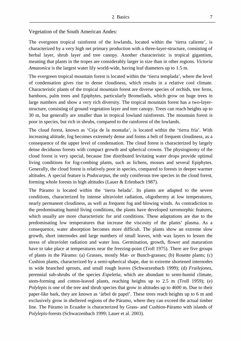
Vegetation of the South American Andes:

The evergreen tropical rainforest of the lowlands, located within the ‘tierra caliente’, is characterized by a very high net primary production with a three-layer-structure, consisting of herbal layer, shrub layer and tree canopy. Another characteristic is tropical gigantism, meaning that plants in the tropes are considerably larger in size than in other regions. Victoria Amazonica is the largest water lily world-wide, having leaf diameters up to 1.5 m.

The evergreen tropical mountain forest is located within the ‘tierra templada’, where the level of condensation gives rise to dense cloudiness, which results in a relative cool climate. Characteristic plants of the tropical mountain forest are diverse species of orchids, tree ferns, bamboos, palm trees and Epiphytes, particularly Bromeliads, which grow on huge trees in large numbers and show a very rich diversity. The tropical mountain forest has a two-layer-structure, consisting of ground vegetation layer and tree canopy. Trees can reach heights up to 30 m, but generally are smaller than in tropical lowland rainforests. The mountain forest is poor in species, but rich in shrubs, compared to the rainforest of the lowlands.

The cloud forest, known as ‘Ceja de la montaña’, is located within the ‘tierra fría’. With increasing altitude, fog becomes extremely dense and forms a belt of frequent cloudiness, as a consequence of the upper level of condensation. The cloud forest is characterized by largely dense deciduous forests with compact growth and spherical crowns. The physiognomy of the cloud forest is very special, because fine distributed levitating water drops provide optimal living conditions for fog-combing plants, such as lichens, mosses and several Epiphytes. Generally, the cloud forest is relatively poor in species, compared to forests in deeper warmer altitudes. A special feature is Podocarpus, the only coniferous tree species in the cloud forest, forming whole forests in high altitudes (Lauer & Erlenbach 1987).

The Páramo is located within the ‘tierra helada’. Its plants are adapted to the severe conditions, characterized by intense ultraviolet radiation, oligothermy at low temperatures, nearly permanent cloudiness, as well as frequent fog and blowing winds. As contradiction to the predominating humid living conditions, the plants have developed xeromorphic features, which usually are more characteristic for arid conditions. These adaptations are due to the predominating low temperatures that increase the viscosity of the plants’ plasma. As a consequence, water absorption becomes more difficult. The plants show an extreme slow growth, short internodes and large numbers of small leaves, with wax layers to lessen the stress of ultraviolet radiation and water loss. Germination, growth, flower and maturation have to take place at temperatures near the freezing-point (Troll 1975). There are five groups of plants in the Páramo: (a) Grasses, mostly Mat- or Bunch-grasses; (b) Rosette plants; (c) Cushion plants, characterized by a semi-spherical shape, due to extreme shortened internodes in wide branched sprouts, and small rough leaves (Schwarzenbach 1999); (d) Frailejones, perennial sub-shrubs of the species Espeletia, which are abundant to semi-humid climate, stem-forming and cotton-leaved plants, reaching heights up to 2.5 m (Troll 1959); (e) Polylepis is one of the tree and shrub species that grow in altitudes up to 4600 m. Due to their paper-like bark, they are known as ‘árbol de papel’. These trees reach heights up to 6 m and exclusively grow in sheltered regions of the Páramo, where they can exceed the actual timber line. The Páramo in Ecuador is characterized by Grass- and Cushion-Páramo with islands of Polylepis-forests (Schwarzenbach 1999; Lauer et al. 2003).

8 2 Basics

Agricultural use and principle of verticality in the South American Andes:

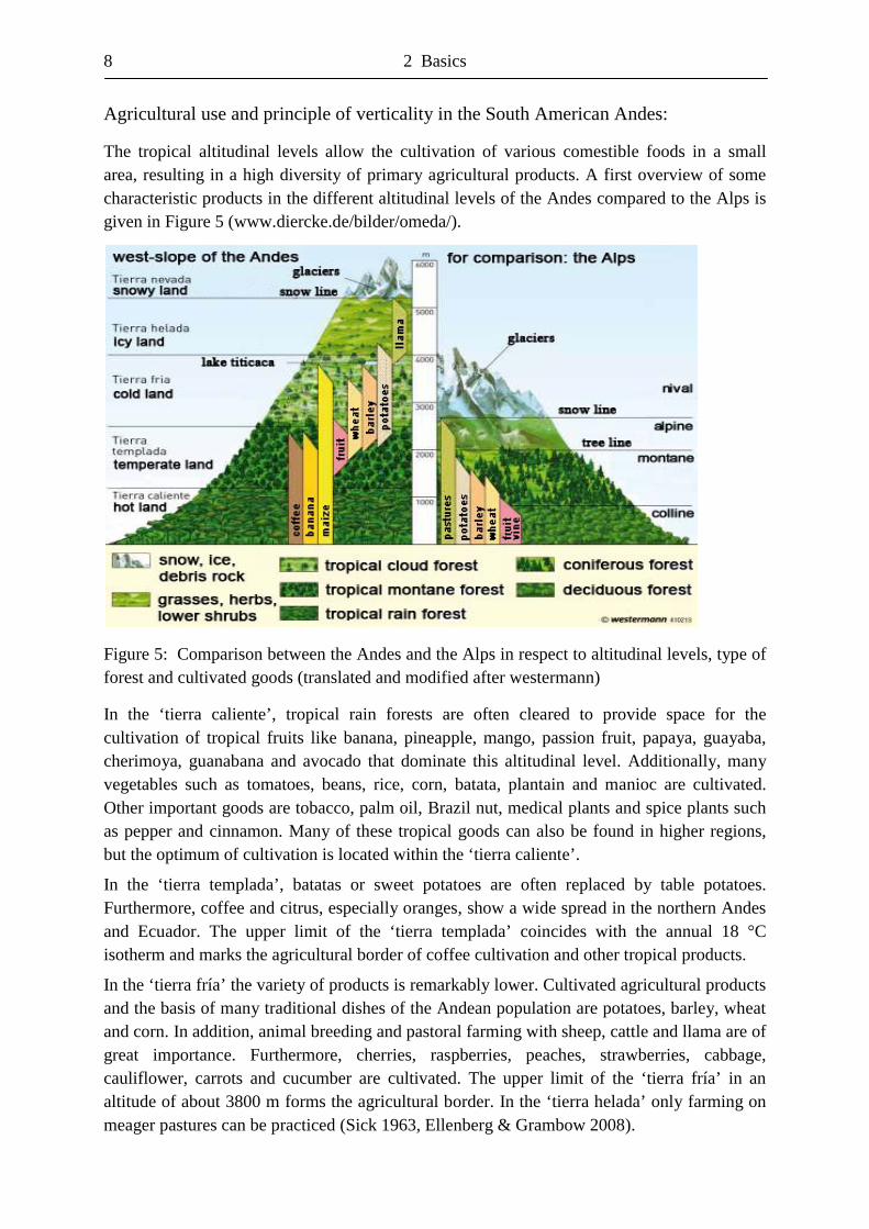
The tropical altitudinal levels allow the cultivation of various comestible foods in a small area, resulting in a high diversity of primary agricultural products. A first overview of some characteristic products in the different altitudinal levels of the Andes compared to the Alps is given in Figure 5 (www.diercke.de/bilder/omeda/).

Figure 5: Comparison between the Andes and the Alps in respect to altitudinal levels, type of forest and cultivated goods (translated and modified after westermann)

In the ‘tierra caliente’, tropical rain forests are often cleared to provide space for the cultivation of tropical fruits like banana, pineapple, mango, passion fruit, papaya, guayaba, cherimoya, guanabana and avocado that dominate this altitudinal level. Additionally, many vegetables such as tomatoes, beans, rice, corn, batata, plantain and manioc are cultivated. Other important goods are tobacco, palm oil, Brazil nut, medical plants and spice plants such as pepper and cinnamon. Many of these tropical goods can also be found in higher regions, but the optimum of cultivation is located within the ‘tierra caliente’.

In the ‘tierra templada’, batatas or sweet potatoes are often replaced by table potatoes. Furthermore, coffee and citrus, especially oranges, show a wide spread in the northern Andes and Ecuador. The upper limit of the ‘tierra templada’ coincides with the annual 18 °C isotherm and marks the agricultural border of coffee cultivation and other tropical products.

In the ‘tierra fría’ the variety of products is remarkably lower. Cultivated agricultural products and the basis of many traditional dishes of the Andean population are potatoes, barley, wheat and corn. In addition, animal breeding and pastoral farming with sheep, cattle and llama are of great importance. Furthermore, cherries, raspberries, peaches, strawberries, cabbage, cauliflower, carrots and cucumber are cultivated. The upper limit of the ‘tierra fría’ in an altitude of about 3800 m forms the agricultural border. In the ‘tierra helada’ only farming on meager pastures can be practiced (Sick 1963, Ellenberg & Grambow 2008).

2 Basics 9

It is remarkable, that the Amazonian lowland rainforest was able to give birth to such a rich biodiversity, although soils on the east-slopes of the Andes are poor in nutrients. As a consequence, the indigenous people have adapted their subsistence strategy. Their traditional agricultural fields, in Quechua are called ‘chacras’, have dimensions up to one ha. Chacras allow the cultivation of a large variety of fruits and vegetables. Traditionally, plants and trees are cultivated in combination due to their variable growing stages, so that there are always certain ripe products that can be harvested. The most important cultivated plant is manioc, followed by corn, plantain, beans, fruits, vegetables, spice plants and medical plants. The cultivation of a chacra takes place in three phases: deforestation, cultivation and fallow. As a chacra can only be cultivated for a few years, due to the exhaustion of the nutrient poor soils, familiar groups have to move and cultivate new chacras in the nearby surroundings. When a chacra is established, trees have to be cleared and shrubs to be burnt. The ashes then provide fertilizer for the nutrient-poor soil. The trees, which remain lying on the ground and their respective stubs, reduce soil erosion and can be used for firewood or new structures. The fallow is necessary for the recovery of the nutrient-poor soils and lasts for 10 - 15 years. Abandoned chacras remain family property and are visited once in a while, to gather wild growing fruits (Gippelhauser & Mader 1990).

Major settlement areas in South America are located in coastal and mountainous regions of the tropical and sub-topical Andes. Nature with its basic physical conditions given climate, bedrock, soil and biological resources, were important selection factors for the early beginnings of human civilisations, originating in high tropical mountains. According to Lauer (1987) pronounced favourable factors for human settlement in the Andes are richness in water and volcanic materials from inner-Andean volcanism, providing not only rich mineral deposits such as S, silver and gold, but also fertile soils. The contrast between the thick nutrient-rich black earths of the highlands such as Kastanozeme and the tropical nutrient-poor red earths of the lowlands such as Acrisole, Laterite und Oxisole is remarkable (Zech 2002). Soil fertility is the basic for the development of enduring agrarian shaped settlements in the Andes. The gain in power of early civilisations is a consequence of overproduction of agricultural goods in the high valleys, sophisticated vertical and horizontal cropping- and trading systems as well as cultural adaption to the three-dimensional differentiation of the unique conditions in the Andes.

Archaeological corpus of funds show that already in paleo-Indian time, a system of stable and wide-ranging trade relations developed within the Andes, extending from the Pacific coast up to the Andean highlands and further to the tropical rainforests of the Amazonian lowland. Beside long-distance trade also spheres of interaction have been developed in correlation with a high geo-ecological biodiversity. Already early cultures of the Andes used the principle of verticality or ecological complementarity, meaning that agrarian products that can be cultivated in a given region, depending on prevailing thermal- and hygric conditions of the different altitudinal levels. The use of these growing areas has created a unique form of settlement and cultivation within families and clans in Andean regions. Generally, traditional trade relations between communities take place through the exchange of goods on markets. Trade contacts today are realised over greater distances due to modern roads that earlier had to take place through the transport of goods via caravans of llama or by foot over the wide-spread net of the Inca-streets of the central Andes (Ellenberg & Grambow 2008).

10 2 Basics

2.4 Deforestation and other Problems in Ecuador

Several scientists estimate that more than 90 % or 25 million ha of Ecuador’s land area had primarily been covered by forests (Cabarle et al. 1989; Wunder 2000). Today, Ecuador suffers the highest rate of deforestation within South America. The average forest cover rate of Ecuador in 2005 was 39 % or 10.8 million ha. The average forest cover rate whole of South America at the same time was 48 % (FAO 2006).

The historical decline of forests in Ecuador can be divided into two major deforestation phases. The persistent deforestation of areas above 1200 m in the ‘Sierra’ during the pre-Columbian era marks the first phase. The second phase was the rapid deforestation of the ‘Costa’ region during the past century. In between these two phases, the dramatic decrease of the indigenous population during the Spanish colonial rule led to a forest expansion. But, the conquest was followed by an intense population pressure on the forests, until the declaration of independence of Ecuador in 1822. From that time on, until the early twentieth century, Ecuador’s forest cover was largely preserved. However, the coastal lowland forests were cleared for agricultural crops during the cocoa boom from 1900 to the end of the 1920s and intensified during the banana boom after the Second World War, with the main period from 1950 to 1965. During the oil boom of the 1970s, roads were built into Ecuador’s Amazon region, the ‘Oriente’, which attracted agricultural colonization and timber extraction (Wunder 2000). Cabarle et al. (1989) estimated the extent of forest in 1958 to be 63 % or 17.4 million ha that dropped remarkably to 45 % or 12.4 million ha in 1987 (FAO 1994). The decline of forests continued from 43 % or 11.9 million ha forest cover in 1990 to 39 % or 10.8 million ha in 2005 (FAO 1994, 2006). In recent years, the area of primary forests remained unchanged, probably due to the protection of many primary forests. 21 % of all forests in Ecuador were protected (UNEP 2002; FAO 2006). Thus, main deforestation today must take place in secondary forests. Current deforestation rates of secondary forests in Ecuador value -1.7 % or a deforested area of 198.000 ha/year (FAO 2006).

These high annual losses are the result of the change in land use from secondary forest to agricultural land. The area of pastures dramatically doubled from 2.2 million ha in 1972 to 4.4 million ha in 1985 with an increase of 244.000 ha/year, and until the end of 1989 to about 6 million ha with an increase of 182.000 ha/year. There are convincing hints that the main forest losses take place in the ‘Sierra’, where cattle ranches are settled (Wunder 2000). Indeed, the forest losses in the ‘Costa’, where commercial crops are cultivated, are lower than in the ‘Sierra’ (Mecham 2001). But this finding also derives from the fact that crop land in the ‘Costa’ only expanded slightly during the period from 1972 to 1989 (Wunder 2000).

While in other countries of South America the conversion of forests is lessened by high reforestation efforts, in Ecuador no substantial areas were reforested. From 2000 to 2005, the plantation area in Ecuador only increased by 560 ha/year (FAO 2006). According to a prediction model of Koopowith et al. (1994), habitat conversion caused by deforestation in Ecuador leads to species extinction rates that range up to 63 species per year.

2 Basics 11

In 1984, Ecuador was one of 19 countries worldwide having large blocks of humid tropical rainforests, and was grouped together with Brazil, Colombia, Indonesia and Malaysia as places with rapid deforestation rates (Office of Technology Assessment 1984; Ledec 1985). In the early 1980s the Ministry of Agriculture, estimated tropical deforestation to be about 183.000 ha/year. A tropical deforestation study between 1977 and 1985, which used remote sensing techniques, estimated the loss of tropical forests to be 340.000 ha/year.

Ecuador has rainforests in the west of the Andes, but most of the rainforests and about half of the country’s land area, are located east of the Andes in the upper reaches of the Amazon basin. In the past, almost all deforestation was located in northern coastal plains, in eastern Andean-slopes, mainly in the province of Morona Santiago and in the northern ‘Oriente’ (Ministerio de Agricultura y Ganaderia 1977). In the ‘Oriente’, oil companies triggered rapid deforestation when they constructed roads to service their wells and pipelines by opening up the areas around Lago Agrio. Thereafter, colonists cleared most of the forests along these roads. The African palm plantations in the north-eastern ‘Oriente’ contributed to the clearance of land only to a minor degree (Carrion & Cuvi 1985). Along Ecuador’s northern coast and in the southern Oriente, timber companies played a significant role in clearing land. However, smallholders working in corridors along the established roads have cleared most of the land, generating similar agrarian structures in these three regions (Barral 1979).

The competition for land between colonists and indigenous peoples characterizes the local politics of these regions (Chiriboga et al. 1989). The same pattern of smallholders’ predominance and colonist-Amerindian conflicts characterizes colonization areas in Rondonia, Brazil and Caqueta, Colombia. In this sense land clearing in Morona Santiago in Ecuador proceeds in a political-economic context. Rapid deforestation did not begin in the Upano-Palora region in Ecuador until the late 1960s, when the construction of the Macas-Puyo road favoured settlement in this region. By the mid-1980s colonists and Shuar had claimed all of the arable land, but much of the land far from roads remained forested.

While the competition between the Shuar and the colonists for control over land explains local variations and short-term fluctuations in deforestation rates, the long-term eastward expansion of settlement depends mainly on activities of growth coalitions and lead institutions, in form of colonization projects. The crucial role of growth coalitions only becomes apparent in detailed histories of the struggles to settle particular places. The clearing of forest remnants in the Upano-Palora Plain in the 1980s illustrates the difficulties of trailblazing and the value of growth coalitions in overcoming obstacles in settlement. Most Upano-Palora smallholders continued to clear land despite these obstacles, but some pushed ahead more vigorously than others. Thus, certain areas show extensive deforestation, while other areas do not (Rudel & Horowitz 1993).

12 2 Basics

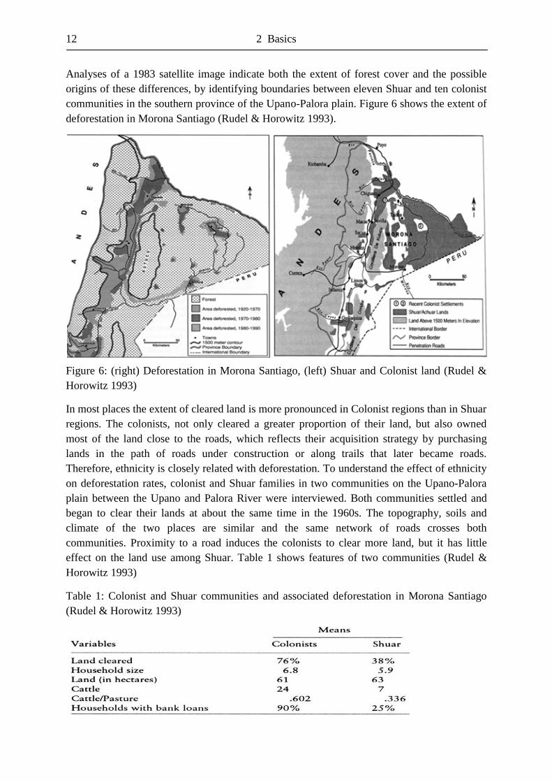
Analyses of a 1983 satellite image indicate both the extent of forest cover and the possible origins of these differences, by identifying boundaries between eleven Shuar and ten colonist communities in the southern province of the Upano-Palora plain. Figure 6 shows the extent of deforestation in Morona Santiago (Rudel & Horowitz 1993).

Figure 6: (right) Deforestation in Morona Santiago, (left) Shuar and Colonist land (Rudel & Horowitz 1993)

In most places the extent of cleared land is more pronounced in Colonist regions than in Shuar regions. The colonists, not only cleared a greater proportion of their land, but also owned most of the land close to the roads, which reflects their acquisition strategy by purchasing lands in the path of roads under construction or along trails that later became roads. Therefore, ethnicity is closely related with deforestation. To understand the effect of ethnicity on deforestation rates, colonist and Shuar families in two communities on the Upano-Palora plain between the Upano and Palora River were interviewed. Both communities settled and began to clear their lands at about the same time in the 1960s. The topography, soils and climate of the two places are similar and the same network of roads crosses both communities. Proximity to a road induces the colonists to clear more land, but it has little effect on the land use among Shuar. Table 1 shows features of two communities (Rudel & Horowitz 1993)

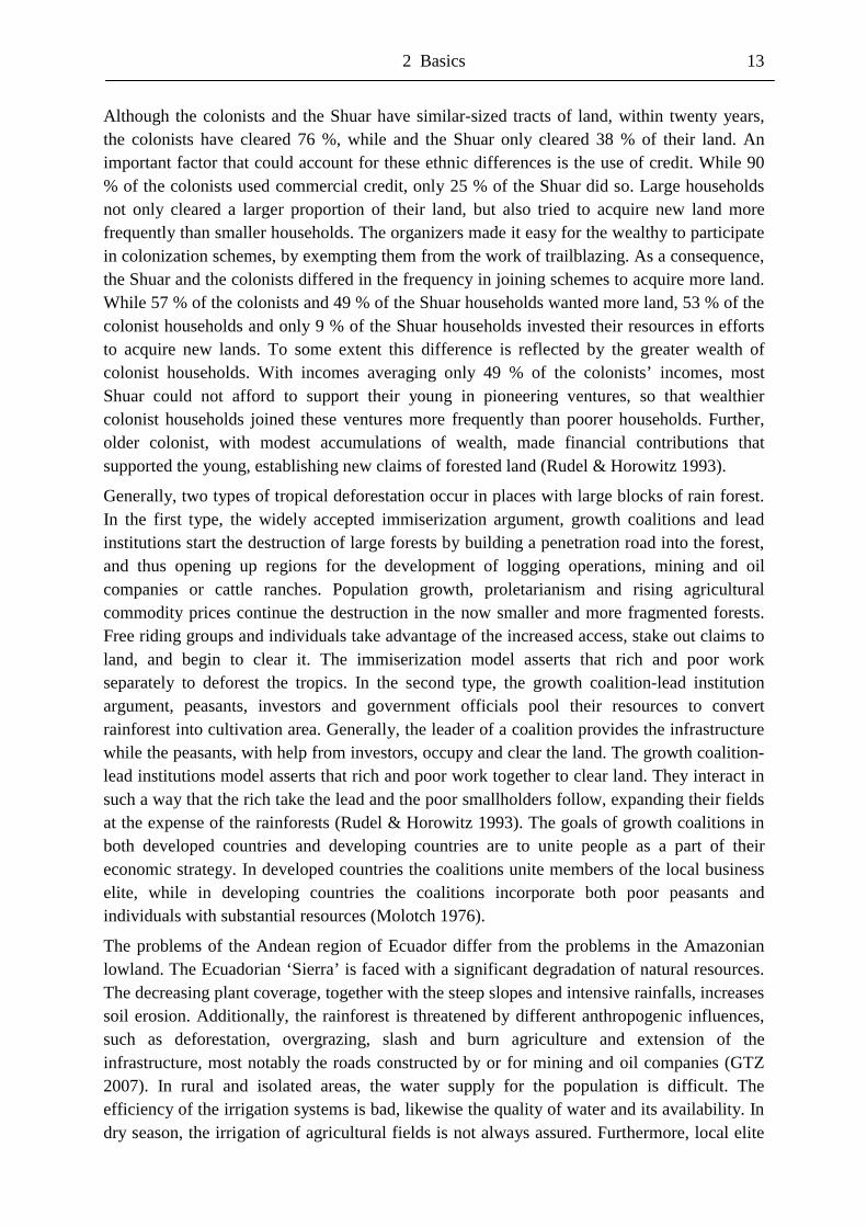
Table 1: Colonist and Shuar communities and associated deforestation in Morona Santiago (Rudel & Horowitz 1993)

2 Basics 13

Although the colonists and the Shuar have similar-sized tracts of land, within twenty years, the colonists have cleared 76 %, while and the Shuar only cleared 38 % of their land. An important factor that could account for these ethnic differences is the use of credit. While 90 % of the colonists used commercial credit, only 25 % of the Shuar did so. Large households not only cleared a larger proportion of their land, but also tried to acquire new land more frequently than smaller households. The organizers made it easy for the wealthy to participate in colonization schemes, by exempting them from the work of trailblazing. As a consequence, the Shuar and the colonists differed in the frequency in joining schemes to acquire more land. While 57 % of the colonists and 49 % of the Shuar households wanted more land, 53 % of the colonist households and only 9 % of the Shuar households invested their resources in efforts to acquire new lands. To some extent this difference is reflected by the greater wealth of colonist households. With incomes averaging only 49 % of the colonists’ incomes, most Shuar could not afford to support their young in pioneering ventures, so that wealthier colonist households joined these ventures more frequently than poorer households. Further, older colonist, with modest accumulations of wealth, made financial contributions that supported the young, establishing new claims of forested land (Rudel & Horowitz 1993).

Generally, two types of tropical deforestation occur in places with large blocks of rain forest. In the first type, the widely accepted immiserization argument, growth coalitions and lead institutions start the destruction of large forests by building a penetration road into the forest, and thus opening up regions for the development of logging operations, mining and oil companies or cattle ranches. Population growth, proletarianism and rising agricultural commodity prices continue the destruction in the now smaller and more fragmented forests. Free riding groups and individuals take advantage of the increased access, stake out claims to land, and begin to clear it. The immiserization model asserts that rich and poor work separately to deforest the tropics. In the second type, the growth coalition-lead institution argument, peasants, investors and government officials pool their resources to convert rainforest into cultivation area. Generally, the leader of a coalition provides the infrastructure while the peasants, with help from investors, occupy and clear the land. The growth coalition-lead institutions model asserts that rich and poor work together to clear land. They interact in such a way that the rich take the lead and the poor smallholders follow, expanding their fields at the expense of the rainforests (Rudel & Horowitz 1993). The goals of growth coalitions in both developed countries and developing countries are to unite people as a part of their economic strategy. In developed countries the coalitions unite members of the local business elite, while in developing countries the coalitions incorporate both poor peasants and individuals with substantial resources (Molotch 1976).

The problems of the Andean region of Ecuador differ from the problems in the Amazonian lowland. The Ecuadorian ‘Sierra’ is faced with a significant degradation of natural resources. The decreasing plant coverage, together with the steep slopes and intensive rainfalls, increases soil erosion. Additionally, the rainforest is threatened by different anthropogenic influences, such as deforestation, overgrazing, slash and burn agriculture and extension of the infrastructure, most notably the roads constructed by or for mining and oil companies (GTZ 2007). In rural and isolated areas, the water supply for the population is difficult. The efficiency of the irrigation systems is bad, likewise the quality of water and its availability. In dry season, the irrigation of agricultural fields is not always assured. Furthermore, local elite

14 2 Basics

groups often claim the water, so that a fair distribution of the available water is often not given (Waldick 2003). This demonstrates the absence and lack of functioning governmental institutions to avoid such social conflicts and enable a just division of water. The rural population furthermore increasingly suffers from shortage in land, due to land purchases and the banishment of small families from fertile land. In the latter case, only steep and difficult to cultivate slopes remain for these families, typically only having an area of 1 - 2 ha per family. Local problems in remote regions also occur due to the absence of infrastructure and a resulting deficient supply of the population (GTZ 2007).

In the Ecuadorian ‘Oriente’, the foundation of new colonies, due to governmental resettlement projects, results in an ever increasing population density. The opening up of sensitive Amazonian rainforest regions, due to the construction of streets and cities, is often accompanied by the invasion of oil- and timber companies as well as agribusinesses appearing out of the nowhere, causing serious environmental destructions, once virgin ecosystems become accessible. Leakages of oil pipelines result in large-scale contaminations of soils and the groundwater. Further, the sensitive soils of the Amazonian lowland are long-lasting disturbed, due to clearance, cattle breeding and the cultivation of cash crop plantations. As a consequence of the increasing population density, pollution, exploitation and cultural differences, conflicts between the indigenous population of the ‘Oriente’ and the new settlers from the highlands come into existence. Often such conflicts arise from unclear circumstances of land rights. However, occasionally controversies also arise within indigenous communities. For example, whole ethnic groups split, as some want to participate in oil business, while the others prefer to continue the traditional way of life. New dependency on economic companies and new wants and needs for goods usually come into existence under westerly influence. The money needed for these goods, partly originates from illegal clearing and selling of tropical wood. Deforestation not only reduces the habitat of animals and plants, but also enables an easier access to the hunting grounds. Thus, a temporal auxiliary income is the vending of meat and fur of wild prey, resulting in over-hunted areas. All in all, the ongoing changes lead to a declining biodiversity and irreversible damages to natural ecosystems and indigenous communities with a traditional way of life (Gippelhauser & Mader 1990).

Many ecosystems within Amazonian rainforest are natural reserves, but international environmental standards, traditional rights of the indigenous people and laws on nature conservations are often not respected, due to weak governmental institutions and a high degree of corruption. Thus, protected natural reserves potentially become cleared, exploited and polluted due to the expansion of infrastructure, deforestation, agribusinesses, mining and contamination through oil companies. In many places, the natural resources of the indigenous people are threatened by such external stressors. In recent years, growing numbers of consolidations of indigenous organisations gained more and more importance on a local, national and international level. However, yet there is no concept for a sustainable development in the Amazonian rainforest. Politics continues the economic way through the promotion of agriculture, infrastructural projects and exploitation of resources, while the protection of the unique biodiversity and culture suffers (Hoffmann 2005).

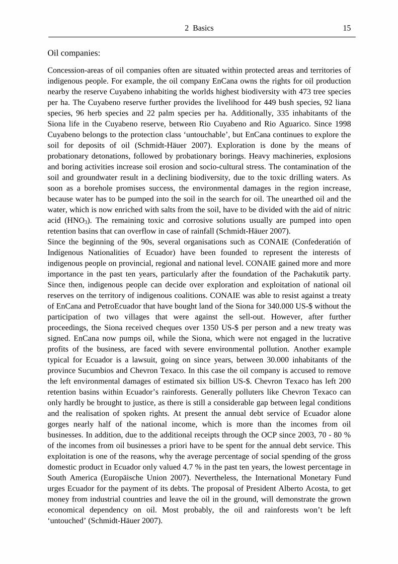
2 Basics 15

Oil companies:

Concession-areas of oil companies often are situated within protected areas and territories of indigenous people. For example, the oil company EnCana owns the rights for oil production nearby the reserve Cuyabeno inhabiting the worlds highest biodiversity with 473 tree species per ha. The Cuyabeno reserve further provides the livelihood for 449 bush species, 92 liana species, 96 herb species and 22 palm species per ha. Additionally, 335 inhabitants of the Siona life in the Cuyabeno reserve, between Rio Cuyabeno and Rio Aguarico. Since 1998 Cuyabeno belongs to the protection class ‘untouchable’, but EnCana continues to explore the soil for deposits of oil (Schmidt-Häuer 2007). Exploration is done by the means of probationary detonations, followed by probationary borings. Heavy machineries, explosions and boring activities increase soil erosion and socio-cultural stress. The contamination of the soil and groundwater result in a declining biodiversity, due to the toxic drilling waters. As soon as a borehole promises success, the environmental damages in the region increase, because water has to be pumped into the soil in the search for oil. The unearthed oil and the water, which is now enriched with salts from the soil, have to be divided with the aid of nitric acid (HNO3). The remaining toxic and corrosive solutions usually are pumped into open retention basins that can overflow in case of rainfall (Schmidt-Häuer 2007).

Since the beginning of the 90s, several organisations such as CONAIE (Confederatión of Indígenous Nationalities of Ecuador) have been founded to represent the interests of indigenous people on provincial, regional and national level. CONAIE gained more and more importance in the past ten years, particularly after the foundation of the Pachakutik party. Since then, indigenous people can decide over exploration and exploitation of national oil reserves on the territory of indigenous coalitions. CONAIE was able to resist against a treaty of EnCana and PetroEcuador that have bought land of the Siona for 340.000 US-$ without the participation of two villages that were against the sell-out. However, after further proceedings, the Siona received cheques over 1350 US-$ per person and a new treaty was signed. EnCana now pumps oil, while the Siona, which were not engaged in the lucrative profits of the business, are faced with severe environmental pollution. Another example typical for Ecuador is a lawsuit, going on since years, between 30.000 inhabitants of the province Sucumbios and Chevron Texaco. In this case the oil company is accused to remove the left environmental damages of estimated six billion US-$. Chevron Texaco has left 200 retention basins within Ecuador’s rainforests. Generally polluters like Chevron Texaco can only hardly be brought to justice, as there is still a considerable gap between legal conditions and the realisation of spoken rights. At present the annual debt service of Ecuador alone gorges nearly half of the national income, which is more than the incomes from oil businesses. In addition, due to the additional receipts through the OCP since 2003, 70 - 80 % of the incomes from oil businesses a priori have to be spent for the annual debt service. This exploitation is one of the reasons, why the average percentage of social spending of the gross domestic product in Ecuador only valued 4.7 % in the past ten years, the lowest percentage in South America (Europäische Union 2007). Nevertheless, the International Monetary Fund urges Ecuador for the payment of its debts. The proposal of President Alberto Acosta, to get money from industrial countries and leave the oil in the ground, will demonstrate the grown economical dependency on oil. Most probably, the oil and rainforests won’t be left ‘untouched’ (Schmidt-Häuer 2007).

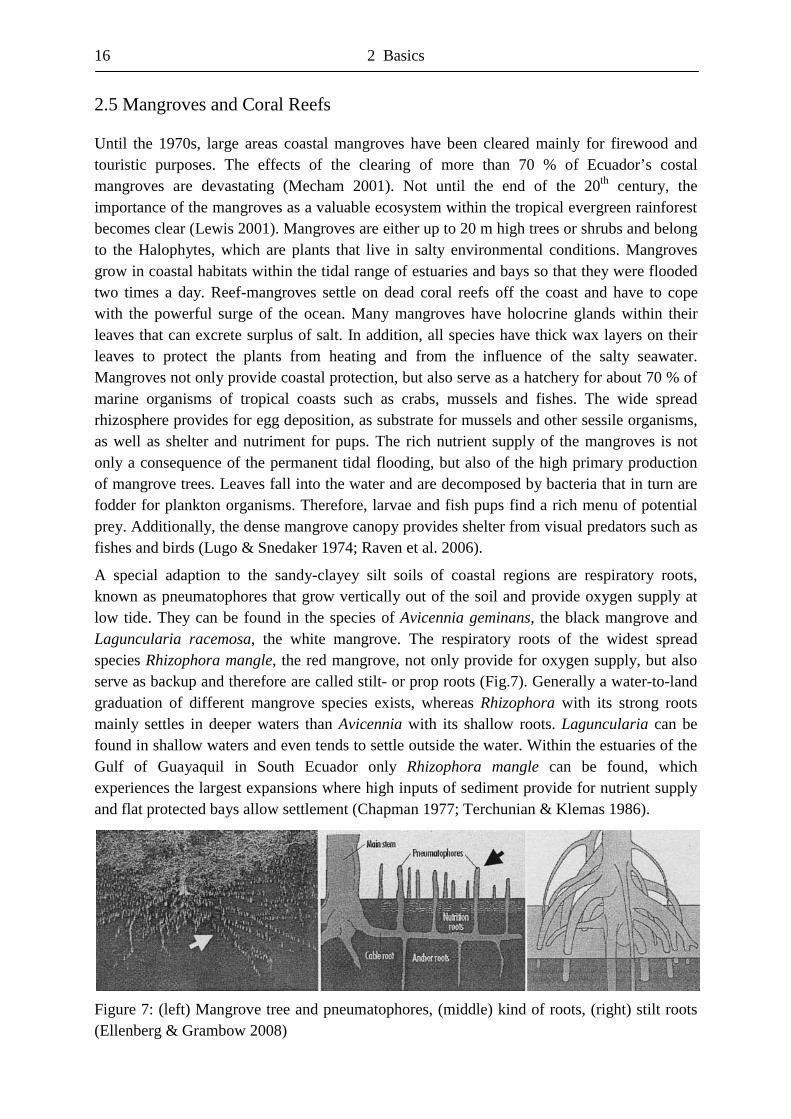
16 2 Basics

2.5 Mangroves and Coral Reefs

Until the 1970s, large areas coastal mangroves have been cleared mainly for firewood and touristic purposes. The effects of the clearing of more than 70 % of Ecuador’s costal mangroves are devastating (Mecham 2001). Not until the end of the 20th century, the importance of the mangroves as a valuable ecosystem within the tropical evergreen rainforest becomes clear (Lewis 2001). Mangroves are either up to 20 m high trees or shrubs and belong to the Halophytes, which are plants that live in salty environmental conditions. Mangroves grow in coastal habitats within the tidal range of estuaries and bays so that they were flooded two times a day. Reef-mangroves settle on dead coral reefs off the coast and have to cope with the powerful surge of the ocean. Many mangroves have holocrine glands within their leaves that can excrete surplus of salt. In addition, all species have thick wax layers on their leaves to protect the plants from heating and from the influence of the salty seawater. Mangroves not only provide coastal protection, but also serve as a hatchery for about 70 % of marine organisms of tropical coasts such as crabs, mussels and fishes. The wide spread rhizosphere provides for egg deposition, as substrate for mussels and other sessile organisms, as well as shelter and nutriment for pups. The rich nutrient supply of the mangroves is not only a consequence of the permanent tidal flooding, but also of the high primary production of mangrove trees. Leaves fall into the water and are decomposed by bacteria that in turn are fodder for plankton organisms. Therefore, larvae and fish pups find a rich menu of potential prey. Additionally, the dense mangrove canopy provides shelter from visual predators such as fishes and birds (Lugo & Snedaker 1974; Raven et al. 2006).

A special adaption to the sandy-clayey silt soils of coastal regions are respiratory roots, known as pneumatophores that grow vertically out of the soil and provide oxygen supply at low tide. They can be found in the species of Avicennia geminans, the black mangrove and Laguncularia racemosa, the white mangrove. The respiratory roots of the widest spread species Rhizophora mangle, the red mangrove, not only provide for oxygen supply, but also serve as backup and therefore are called stilt- or prop roots (Fig.7). Generally a water-to-land graduation of different mangrove species exists, whereas Rhizophora with its strong roots mainly settles in deeper waters than Avicennia with its shallow roots. Laguncularia can be found in shallow waters and even tends to settle outside the water. Within the estuaries of the Gulf of Guayaquil in South Ecuador only Rhizophora mangle can be found, which experiences the largest expansions where high inputs of sediment provide for nutrient supply and flat protected bays allow settlement (Chapman 1977; Terchunian & Klemas 1986).

Figure 7: (left) Mangrove tree and pneumatophores, (middle) kind of roots, (right) stilt roots (Ellenberg & Grambow 2008)

2 Basics 17

Mangroves are able to cope with extreme living conditions and therefore occur in almost all tropical coastal regions around the world and even in sub-tropical coastal regions like in Florida and New Zealand. However, mangroves are abundant to flat coastal regions, high nutrient inputs as well as constant average air- and water-temperatures above 18 °C with maximum diurnal variations of ± 5 °C. Further, an annual precipitation of 2000 - 5000 mm with a minimum of 100 mm per month is essential (Frey & Lösch 2004). Figure 8 shows the geographic range of about 17 million ha of worldwide existing mangroves (FAO 2003).

Figure 8: Geographic range of mangroves (modified after Ellenberg & Grambow 2008)

There is a strong negative correlation between the occurrence of cold sea currents and the geographic range of mangrove areas. This climatic dependence can be observed in the west-coast of South America, where the cold Humboldt stream prohibits a further southward extension of mangroves along the Peruvian coast. The same effect can be observed in South-West Africa, where the influence of the cold Bengal stream prohibits a further southward extension of the mangroves at the latitude of Angola (Terchunian & Klemas 1986).

Generally, mangroves considerably slow down flow velocity due to their dense rhizosphere, so that sediments and nutrients accumulate within the tidal range of estuaries and deltas. Therefore, nutrients and fine substrates can’t reach the ocean, where coral reefs are situated, like in the case of the Great Barrier Reef in Australia. It has to be mentioned, that coral reefs exclusively can exist in oligotroph, which means nutrient-poor, water. Indeed, most of the rivers in estuaries provide for rich nutrient supply and large amounts of sediments.

Therefore, when existing mangroves are cleared, large amounts of sediments can be accumulated on coral reefs. Similarly a surplus of nutrients can increase the growth of algae, which compete with the symbiotic community of the coral reef for sunlight. As a consequence of both processes, the whole coral reef could die, because of the lack of sunlight that is needed for photosynthesis. According to this, there is a tight connection between the ecosystems of coral reefs and mangroves that provide essential filtering processes for the existence of coral reefs (Baran & Hambrey 1998).

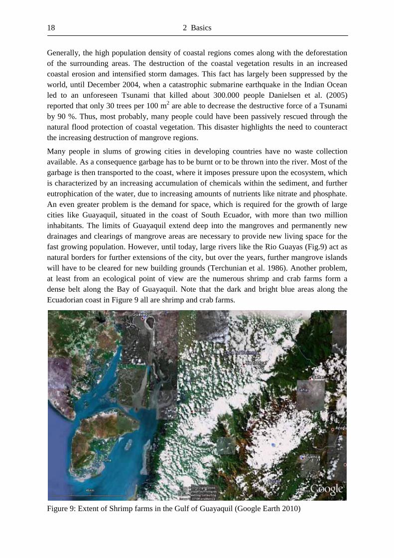
18 2 Basics

Generally, the high population density of coastal regions comes along with the deforestation of the surrounding areas. The destruction of the coastal vegetation results in an increased coastal erosion and intensified storm damages. This fact has largely been suppressed by the world, until December 2004, when a catastrophic submarine earthquake in the Indian Ocean led to an unforeseen Tsunami that killed about 300.000 people Danielsen et al. (2005) reported that only 30 trees per 100 m2 are able to decrease the destructive force of a Tsunami by 90 %. Thus, most probably, many people could have been passively rescued through the natural flood protection of coastal vegetation. This disaster highlights the need to counteract the increasing destruction of mangrove regions.

Many people in slums of growing cities in developing countries have no waste collection available. As a consequence garbage has to be burnt or to be thrown into the river. Most of the garbage is then transported to the coast, where it imposes pressure upon the ecosystem, which is characterized by an increasing accumulation of chemicals within the sediment, and further eutrophication of the water, due to increasing amounts of nutrients like nitrate and phosphate. An even greater problem is the demand for space, which is required for the growth of large cities like Guayaquil, situated in the coast of South Ecuador, with more than two million inhabitants. The limits of Guayaquil extend deep into the mangroves and permanently new drainages and clearings of mangrove areas are necessary to provide new living space for the fast growing population. However, until today, large rivers like the Rio Guayas (Fig.9) act as natural borders for further extensions of the city, but over the years, further mangrove islands will have to be cleared for new building grounds (Terchunian et al. 1986). Another problem, at least from an ecological point of view are the numerous shrimp and crab farms form a dense belt along the Bay of Guayaquil. Note that the dark and bright blue areas along the Ecuadorian coast in Figure 9 all are shrimp and crab farms.

Figure 9: Extent of Shrimp farms in the Gulf of Guayaquil (Google Earth 2010)

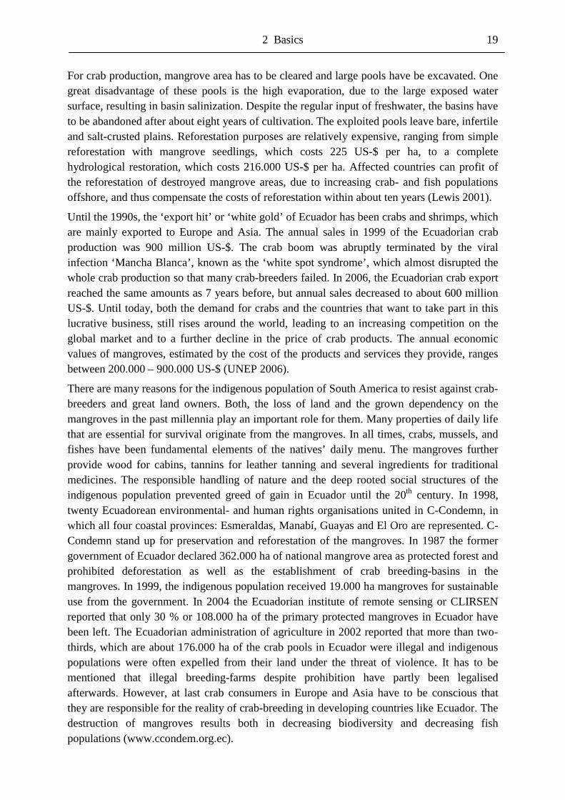
2 Basics 19

For crab production, mangrove area has to be cleared and large pools have be excavated. One great disadvantage of these pools is the high evaporation, due to the large exposed water surface, resulting in basin salinization. Despite the regular input of freshwater, the basins have to be abandoned after about eight years of cultivation. The exploited pools leave bare, infertile and salt-crusted plains. Reforestation purposes are relatively expensive, ranging from simple reforestation with mangrove seedlings, which costs 225 US-$ per ha, to a complete hydrological restoration, which costs 216.000 US-$ per ha. Affected countries can profit of the reforestation of destroyed mangrove areas, due to increasing crab- and fish populations offshore, and thus compensate the costs of reforestation within about ten years (Lewis 2001).

Until the 1990s, the ‘export hit’ or ‘white gold’ of Ecuador has been crabs and shrimps, which are mainly exported to Europe and Asia. The annual sales in 1999 of the Ecuadorian crab production was 900 million US-$. The crab boom was abruptly terminated by the viral infection ‘Mancha Blanca’, known as the ‘white spot syndrome’, which almost disrupted the whole crab production so that many crab-breeders failed. In 2006, the Ecuadorian crab export reached the same amounts as 7 years before, but annual sales decreased to about 600 million US-$. Until today, both the demand for crabs and the countries that want to take part in this lucrative business, still rises around the world, leading to an increasing competition on the global market and to a further decline in the price of crab products. The annual economic values of mangroves, estimated by the cost of the products and services they provide, ranges between 200.000 – 900.000 US-$ (UNEP 2006).

There are many reasons for the indigenous population of South America to resist against crab-breeders and great land owners. Both, the loss of land and the grown dependency on the mangroves in the past millennia play an important role for them. Many properties of daily life that are essential for survival originate from the mangroves. In all times, crabs, mussels, and fishes have been fundamental elements of the natives’ daily menu. The mangroves further provide wood for cabins, tannins for leather tanning and several ingredients for traditional medicines. The responsible handling of nature and the deep rooted social structures of the indigenous population prevented greed of gain in Ecuador until the 20th century. In 1998, twenty Ecuadorean environmental- and human rights organisations united in C-Condemn, in which all four coastal provinces: Esmeraldas, Manabí, Guayas and El Oro are represented. C-Condemn stand up for preservation and reforestation of the mangroves. In 1987 the former government of Ecuador declared 362.000 ha of national mangrove area as protected forest and prohibited deforestation as well as the establishment of crab breeding-basins in the mangroves. In 1999, the indigenous population received 19.000 ha mangroves for sustainable use from the government. In 2004 the Ecuadorian institute of remote sensing or CLIRSEN reported that only 30 % or 108.000 ha of the primary protected mangroves in Ecuador have been left. The Ecuadorian administration of agriculture in 2002 reported that more than two-thirds, which are about 176.000 ha of the crab pools in Ecuador were illegal and indigenous populations were often expelled from their land under the threat of violence. It has to be mentioned that illegal breeding-farms despite prohibition have partly been legalised afterwards. However, at last crab consumers in Europe and Asia have to be conscious that they are responsible for the reality of crab-breeding in developing countries like Ecuador. The destruction of mangroves results both in decreasing biodiversity and decreasing fish populations (www.ccondem.org.ec).

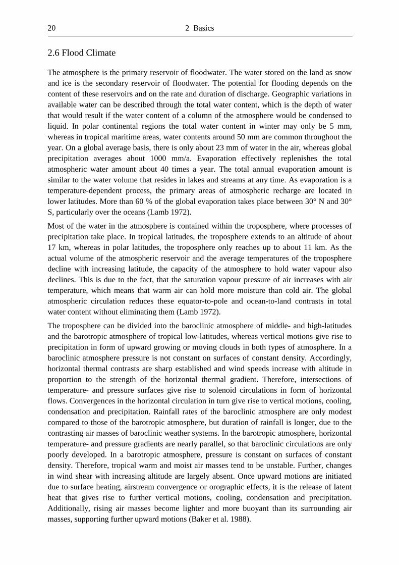
20 2 Basics

2.6 Flood Climate

The atmosphere is the primary reservoir of floodwater. The water stored on the land as snow and ice is the secondary reservoir of floodwater. The potential for flooding depends on the content of these reservoirs and on the rate and duration of discharge. Geographic variations in available water can be described through the total water content, which is the depth of water that would result if the water content of a column of the atmosphere would be condensed to liquid. In polar continental regions the total water content in winter may only be 5 mm, whereas in tropical maritime areas, water contents around 50 mm are common throughout the year. On a global average basis, there is only about 23 mm of water in the air, whereas global precipitation averages about 1000 mm/a. Evaporation effectively replenishes the total atmospheric water amount about 40 times a year. The total annual evaporation amount is similar to the water volume that resides in lakes and streams at any time. As evaporation is a temperature-dependent process, the primary areas of atmospheric recharge are located in lower latitudes. More than 60 % of the global evaporation takes place between 30° N and 30° S, particularly over the oceans (Lamb 1972).

Most of the water in the atmosphere is contained within the troposphere, where processes of precipitation take place. In tropical latitudes, the troposphere extends to an altitude of about 17 km, whereas in polar latitudes, the troposphere only reaches up to about 11 km. As the actual volume of the atmospheric reservoir and the average temperatures of the troposphere decline with increasing latitude, the capacity of the atmosphere to hold water vapour also declines. This is due to the fact, that the saturation vapour pressure of air increases with air temperature, which means that warm air can hold more moisture than cold air. The global atmospheric circulation reduces these equator-to-pole and ocean-to-land contrasts in total water content without eliminating them (Lamb 1972).

The troposphere can be divided into the baroclinic atmosphere of middle- and high-latitudes and the barotropic atmosphere of tropical low-latitudes, whereas vertical motions give rise to precipitation in form of upward growing or moving clouds in both types of atmosphere. In a baroclinic atmosphere pressure is not constant on surfaces of constant density. Accordingly, horizontal thermal contrasts are sharp established and wind speeds increase with altitude in proportion to the strength of the horizontal thermal gradient. Therefore, intersections of temperature- and pressure surfaces give rise to solenoid circulations in form of horizontal flows. Convergences in the horizontal circulation in turn give rise to vertical motions, cooling, condensation and precipitation. Rainfall rates of the baroclinic atmosphere are only modest compared to those of the barotropic atmosphere, but duration of rainfall is longer, due to the contrasting air masses of baroclinic weather systems. In the barotropic atmosphere, horizontal temperature- and pressure gradients are nearly parallel, so that baroclinic circulations are only poorly developed. In a barotropic atmosphere, pressure is constant on surfaces of constant density. Therefore, tropical warm and moist air masses tend to be unstable. Further, changes in wind shear with increasing altitude are largely absent. Once upward motions are initiated due to surface heating, airstream convergence or orographic effects, it is the release of latent heat that gives rise to further vertical motions, cooling, condensation and precipitation. Additionally, rising air masses become lighter and more buoyant than its surrounding air masses, supporting further upward motions (Baker et al. 1988).

2 Basics 21

This auto-convective process sustains vertical motions in the surface layer that can give rise to gigantic cumulonimbus clouds. These convective clouds, which represent the basic rainmaking elements in the barotropic atmosphere, can grow as great and nearly vertical chimneys, as they were not sheared off by strong winds aloft. Horizontal convergence and heating in the surface layer of the barotropic atmosphere gives rise to the vertical motions needed to support condensation and precipitation. As a consequence, convection through a deep layer of the atmosphere is possible, high rainfall rates of short duration can be generated. Thus discharges originating from the atmospheric reservoir differ remarkably between the barotropic- and baroclinic atmosphere. However, sufficient rainfall amounts to cause flooding depend on advection, convergence and upward motions of moisture (Lamb 1972).

The dominant rain-producing organized weather systems of the barotropic low latitudes are: the Inter-tropical Convergence Zone (ITCZ), cyclonic motions and curvatures of the pressure field, such as tropical storms and easterly waves, and orographic uplift processes.

The ITCZ is a circum-equatorial band of cloudiness that originates from the convergence of the trade wind streams of the Northern and Southern hemisphere, and is sometimes referred to as the ‘meteorological equator’, ‘belt of equatorial calms’ or the ‘doldrums’. This belt of convergence underlies a regular annual north-south excursion that is in its most northward position during Northern Hemisphere summer and in its most southward position during Southern Hemisphere summer. Figure 10 shows the position of the ITCZ and the 25 mm atmospheric water content contours in January and July (Lamb 1972).

Figure 10: Position of the ITCZ (lower dotted line) in January and (upper dotted line) in July, after Atkinson & Sadler (1970); 25-mm atmospheric water content contours (dashed lines) in January, mean winter and (solid lines) in July, mean summer, after Lamb (1972).

The 25-mm contours of the total atmospheric water content in January and July mark the transition zone between barotropic low-latitude and baroclinic high-latitude atmospheres. The lines follow that of Lamb (1972), except for the adjusted contour in the area of North Africa, where the atmospheric water content is below 25 mm. Therefore the air in North and East Africa, the Outback of Australia, the southern coast of the Arabian Peninsula and the Rajasthan desert of northwest India is moist enough to support considerable rainfall, although rainfall is often not realized, as the strength of convergence is too weak to initiate, support and sustain vertical motions, so that only slight rainfall results and the regions tend to be arid.

22 2 Basics

Where highlands are present in these regions, uplift is enhanced by orographic processes, resulting in great rainfall amounts. For example, most of the rainfall amounts that give rise to Nile flooding originates from the Ethiopian highlands as the ITCZ passes northward during the Northern Hemisphere summer. In years when the convergence fails to penetrate that far north, droughts, such as the drought and famine from 1981 to 1985 occur in the region.

As a consequence of the latitudinal movement of the ITCZ, a pronounced seasonality in rainfall results over much of the tropical regions. The 25-mm contour in July clearly indicates the monsoon invasion of moist air in eastern Asia, and the midsummer penetration of maritime tropical air into the high plains of North America. The common term monsoon is often associated to summer rainy seasons, while the specific term Monsoon is reserved for the pronounced Asian monsoon. In Cerrapunji, India, the record of 26.461 mm annual rainfall in 1860/61, as well as the record of 9300 mm monthly rainfall in July 1861 was dated. In another Monsoon, rainfall volume was 2500 mm in 100 hours. Off the west coast of South America the normal seasonal excursions of the ITCZ encompass only a few degrees of latitude and are largely confined to Colombia and Ecuador. In years of El Niño, warm tropical sea water extends southward along the coast, resulting in heavy convective rainfalls and flooding in the arid Peruvian and Ecuadorian coasts (Baker et al. 1988).

The 25-mm contours delimit regions with modest rainfall rates of long duration from regions with high rainfall rates of short duration. The boundary between the baroclinic- and barotropic atmosphere is approximately the northern limit of tropical air masses and varies on both seasonal and synoptic time scales. Three broad zones can be defined: The perennial baroclinic zone of the high latitudes, where water content is generally less than 25 mm throughout the year; The perennial barotropic zone of the low latitudes, where the water content exceeds 25 mm all year; The barotropic and baroclinic zone of the middle latitudes, which conditions alternate depending on season and synoptic time scales (Baker et al. 1988).

Thunderstorms are fully matured convective systems and commonly occur in perennial and seasonal barotropic conditions. Populations of thunderstorms are often organized into larger scale assemblages of convective weather elements. Figure 11 shows the global distribution and frequency of annual thunderstorms (Lamb 1972).

Figure 11: Frequency of annual thunderstorms: (black) regions with 100 or more thunder-storms per year, (dotted lines) encompass regions with more than 50 thunderstorms per year, (dashed-dotted lines) encompass regions with at least 20 thunderstorms per year (Lamb 1972)

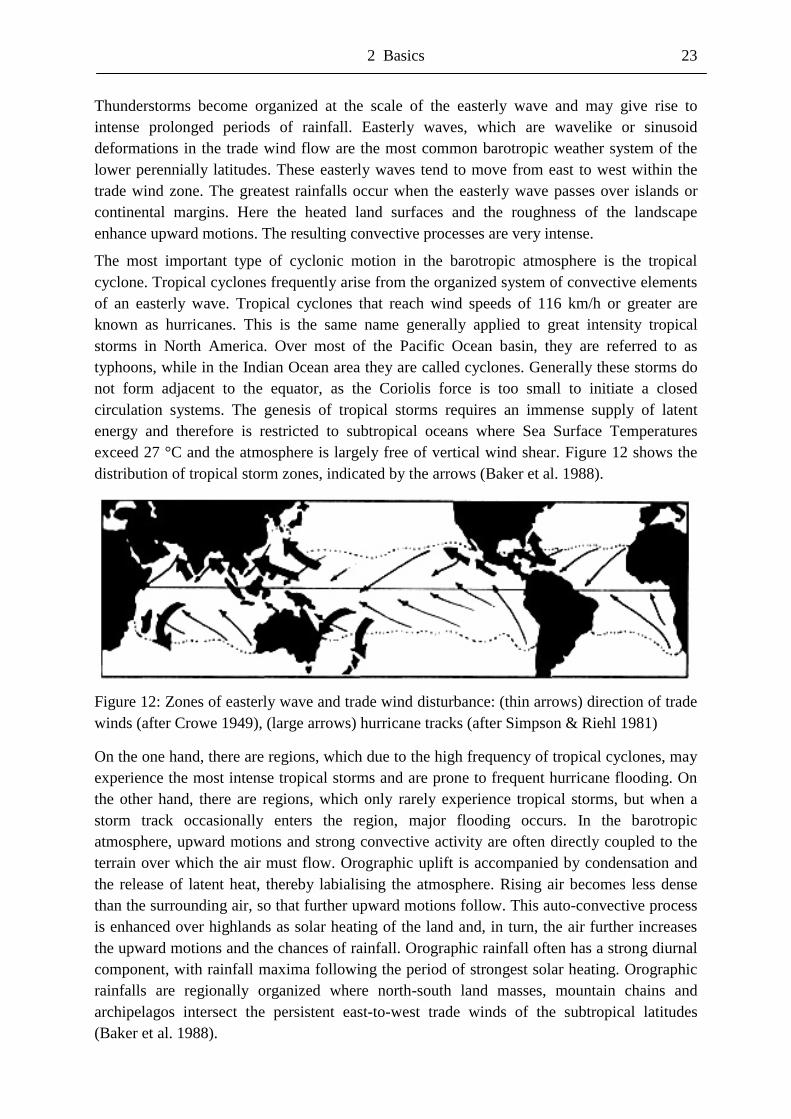
2 Basics 23

Thunderstorms become organized at the scale of the easterly wave and may give rise to intense prolonged periods of rainfall. Easterly waves, which are wavelike or sinusoid deformations in the trade wind flow are the most common barotropic weather system of the lower perennially latitudes. These easterly waves tend to move from east to west within the trade wind zone. The greatest rainfalls occur when the easterly wave passes over islands or continental margins. Here the heated land surfaces and the roughness of the landscape enhance upward motions. The resulting convective processes are very intense.

The most important type of cyclonic motion in the barotropic atmosphere is the tropical cyclone. Tropical cyclones frequently arise from the organized system of convective elements of an easterly wave. Tropical cyclones that reach wind speeds of 116 km/h or greater are known as hurricanes. This is the same name generally applied to great intensity tropical storms in North America. Over most of the Pacific Ocean basin, they are referred to as typhoons, while in the Indian Ocean area they are called cyclones. Generally these storms do not form adjacent to the equator, as the Coriolis force is too small to initiate a closed circulation systems. The genesis of tropical storms requires an immense supply of latent energy and therefore is restricted to subtropical oceans where Sea Surface Temperatures exceed 27 °C and the atmosphere is largely free of vertical wind shear. Figure 12 shows the distribution of tropical storm zones, indicated by the arrows (Baker et al. 1988).

Figure 12: Zones of easterly wave and trade wind disturbance: (thin arrows) direction of trade winds (after Crowe 1949), (large arrows) hurricane tracks (after Simpson & Riehl 1981)

On the one hand, there are regions, which due to the high frequency of tropical cyclones, may experience the most intense tropical storms and are prone to frequent hurricane flooding. On the other hand, there are regions, which only rarely experience tropical storms, but when a storm track occasionally enters the region, major flooding occurs. In the barotropic atmosphere, upward motions and strong convective activity are often directly coupled to the terrain over which the air must flow. Orographic uplift is accompanied by condensation and the release of latent heat, thereby labialising the atmosphere. Rising air becomes less dense than the surrounding air, so that further upward motions follow. This auto-convective process is enhanced over highlands as solar heating of the land and, in turn, the air further increases the upward motions and the chances of rainfall. Orographic rainfall often has a strong diurnal component, with rainfall maxima following the period of strongest solar heating. Orographic rainfalls are regionally organized where north-south land masses, mountain chains and archipelagos intersect the persistent east-to-west trade winds of the subtropical latitudes (Baker et al. 1988).

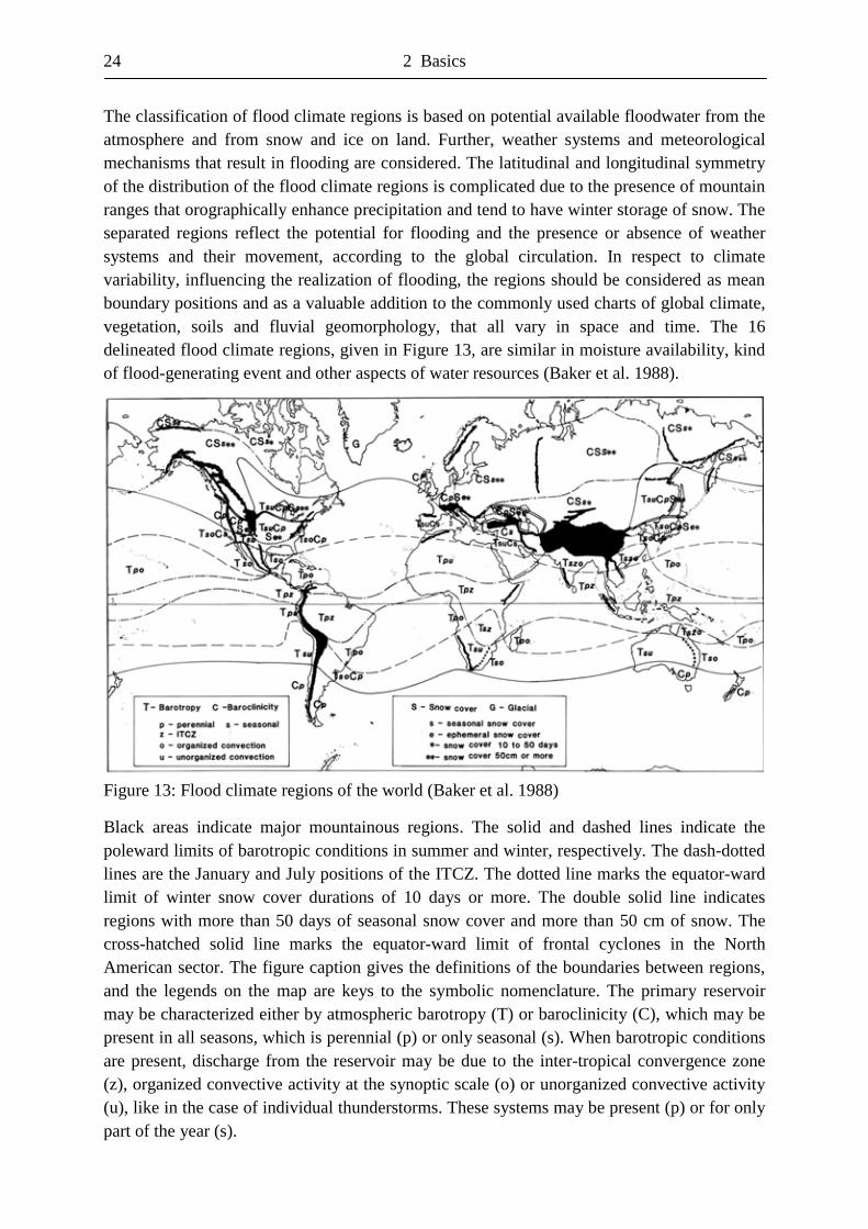
24 2 Basics

The classification of flood climate regions is based on potential available floodwater from the atmosphere and from snow and ice on land. Further, weather systems and meteorological mechanisms that result in flooding are considered. The latitudinal and longitudinal symmetry of the distribution of the flood climate regions is complicated due to the presence of mountain ranges that orographically enhance precipitation and tend to have winter storage of snow. The separated regions reflect the potential for flooding and the presence or absence of weather systems and their movement, according to the global circulation. In respect to climate variability, influencing the realization of flooding, the regions should be considered as mean boundary positions and as a valuable addition to the commonly used charts of global climate, vegetation, soils and fluvial geomorphology, that all vary in space and time. The 16 delineated flood climate regions, given in Figure 13, are similar in moisture availability, kind of flood-generating event and other aspects of water resources (Baker et al. 1988).

Figure 13: Flood climate regions of the world (Baker et al. 1988)

Black areas indicate major mountainous regions. The solid and dashed lines indicate the poleward limits of barotropic conditions in summer and winter, respectively. The dash-dotted lines are the January and July positions of the ITCZ. The dotted line marks the equator-ward limit of winter snow cover durations of 10 days or more. The double solid line indicates regions with more than 50 days of seasonal snow cover and more than 50 cm of snow. The cross-hatched solid line marks the equator-ward limit of frontal cyclones in the North American sector. The figure caption gives the definitions of the boundaries between regions, and the legends on the map are keys to the symbolic nomenclature. The primary reservoir may be characterized either by atmospheric barotropy (T) or baroclinicity (C), which may be present in all seasons, which is perennial (p) or only seasonal (s). When barotropic conditions are present, discharge from the reservoir may be due to the inter-tropical convergence zone (z), organized convective activity at the synoptic scale (o) or unorganized convective activity (u), like in the case of individual thunderstorms. These systems may be present (p) or for only part of the year (s).

2 Basics 25

In high altitudes of the baroclinic atmosphere, where rainfall intensity and totals are modest, the accumulation of snow on the surface (S) is the main trigger mechanism of flooding. When snow accumulates over the winter and melts in the spring, the subscript (s) is used and indicates seasonal snowmelt and flooding. When the accumulated snow is discharged within the winter season on a periodic basis, the subscript (e) is used and indicates the ephemeral nature of the snow cover in this reservoir. The potential for flooding at the end of the winter snow accumulation season is dependent on the depth of snow cover. Areas with sufficient snow cover of 50 cm or more are indicated by double asterisks (**) and areas with less than 50 cm snow cover by single asterisk (*).

Tpo regions are barotropic all year, situated within the trade wind zone pole-ward of the seasonal limits of the ITCZ and encompass many islands. Organized systems of convective elements, such as easterly waves in the trade wind streams and tropical storms give rise to rainfalls in these regions. Orography and heated land surfaces are important forcing process in the initiation of precipitation, resulting in flooding. Tpo regions tend to have a strong diurnal cycle in rainfall where rainfalls are most common in the late afternoon and just after sunset.

Tpu regions, such as Ecuador, are barotropic perennial all year and both easterly waves and tropical storms are uncommon or absent. Therefore, convective elements usually are discrete and/or individual thunderstorms. Generally these regions are semi-arid to arid and accordingly streams frequently ephemeral. However, where mountains occur in these regions, orography is an important factor for the initiation of precipitation and unusual atmospheric conditions may produce flooding. Along the coast of Peru, periods without sufficient rainfall to cause flooding can last for decades. However, as the ITCZ moves unusually far to the south, which is common in years of El Niño, when warm water extends southward along the Peruvian coast, heavy flooding occurs as the landscape is not adjusted to such rainfall events.

Tpz regions are perennially barotropic, situated nearby the equator and the ITCZ that provides the upward motions needed to initiate precipitation. Usually, a rainy season and a drier season are established due to the north-south movement of the ITCZ. The exception to this seasonality occurs along the west coast of South America in Colombia, where the north-south excursions of the ITCZ are small and it is rainy throughout the year. While the zone is circum-global, there are strong longitudinal variations in the amount of precipitation realized as the ITCZ is not equally active at all longitudes (Baker et al. 1988).

These flood climate regions bear considerable similarity to charts of vegetation cover classes based on climatic relationships (Emanuel et al. 1985) as well as to standard classifications of vegetation cover (Udvardy 1975). This is due to the fact that vegetation cover is a function of rainfall, temperature, snow cover, and the seasonality of these parameters. Furthermore, similarities with traditional climate classifications of Köppen (1936) and Trewartha (1968), in which temperature plays a major role, are obvious. This is due to the fact that barotropic and baroclinic conditions of the atmosphere act as a substitute of temperature. Similarities to the classification of the climate of the ocean by Dietrich (1963), the classification of coastal and marine regions of the world by Hayden et al. (1984) and the classification of North American climates based on air masses and streamlines by Bryson (1996) are especially encouraging. All mentioned classifications had the destiny of a classification based on atmospheric dynamics (Baker et al. 1988).

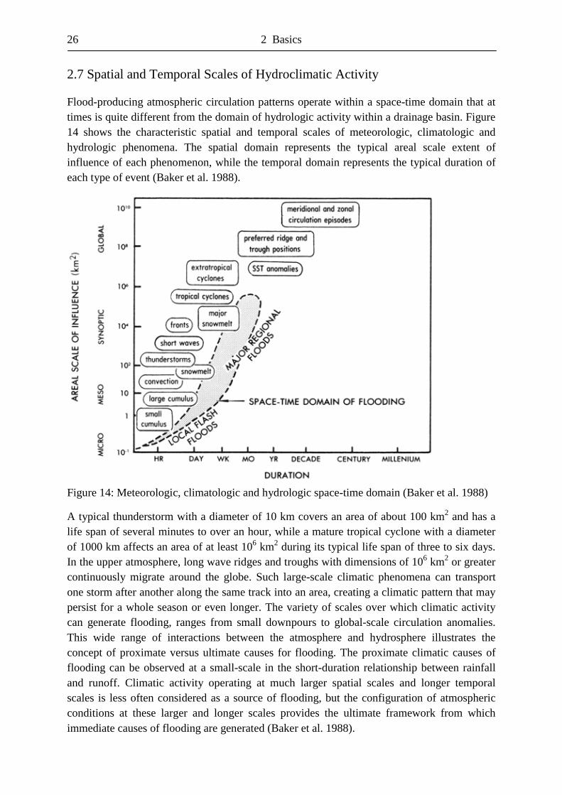
26 2 Basics

2.7 Spatial and Temporal Scales of Hydroclimatic Activity

Flood-producing atmospheric circulation patterns operate within a space-time domain that at times is quite different from the domain of hydrologic activity within a drainage basin. Figure 14 shows the characteristic spatial and temporal scales of meteorologic, climatologic and hydrologic phenomena. The spatial domain represents the typical areal scale extent of influence of each phenomenon, while the temporal domain represents the typical duration of each type of event (Baker et al. 1988).

Figure 14: Meteorologic, climatologic and hydrologic space-time domain (Baker et al. 1988)

A typical thunderstorm with a diameter of 10 km covers an area of about 100 km2 and has a life span of several minutes to over an hour, while a mature tropical cyclone with a diameter of 1000 km affects an area of at least 106 km2 during its typical life span of three to six days. In the upper atmosphere, long wave ridges and troughs with dimensions of 106 km2 or greater continuously migrate around the globe. Such large-scale climatic phenomena can transport one storm after another along the same track into an area, creating a climatic pattern that may persist for a whole season or even longer. The variety of scales over which climatic activity can generate flooding, ranges from small downpours to global-scale circulation anomalies. This wide range of interactions between the atmosphere and hydrosphere illustrates the concept of proximate versus ultimate causes for flooding. The proximate climatic causes of flooding can be observed at a small-scale in the short-duration relationship between rainfall and runoff. Climatic activity operating at much larger spatial scales and longer temporal scales is less often considered as a source of flooding, but the configuration of atmospheric conditions at these larger and longer scales provides the ultimate framework from which immediate causes of flooding are generated (Baker et al. 1988).

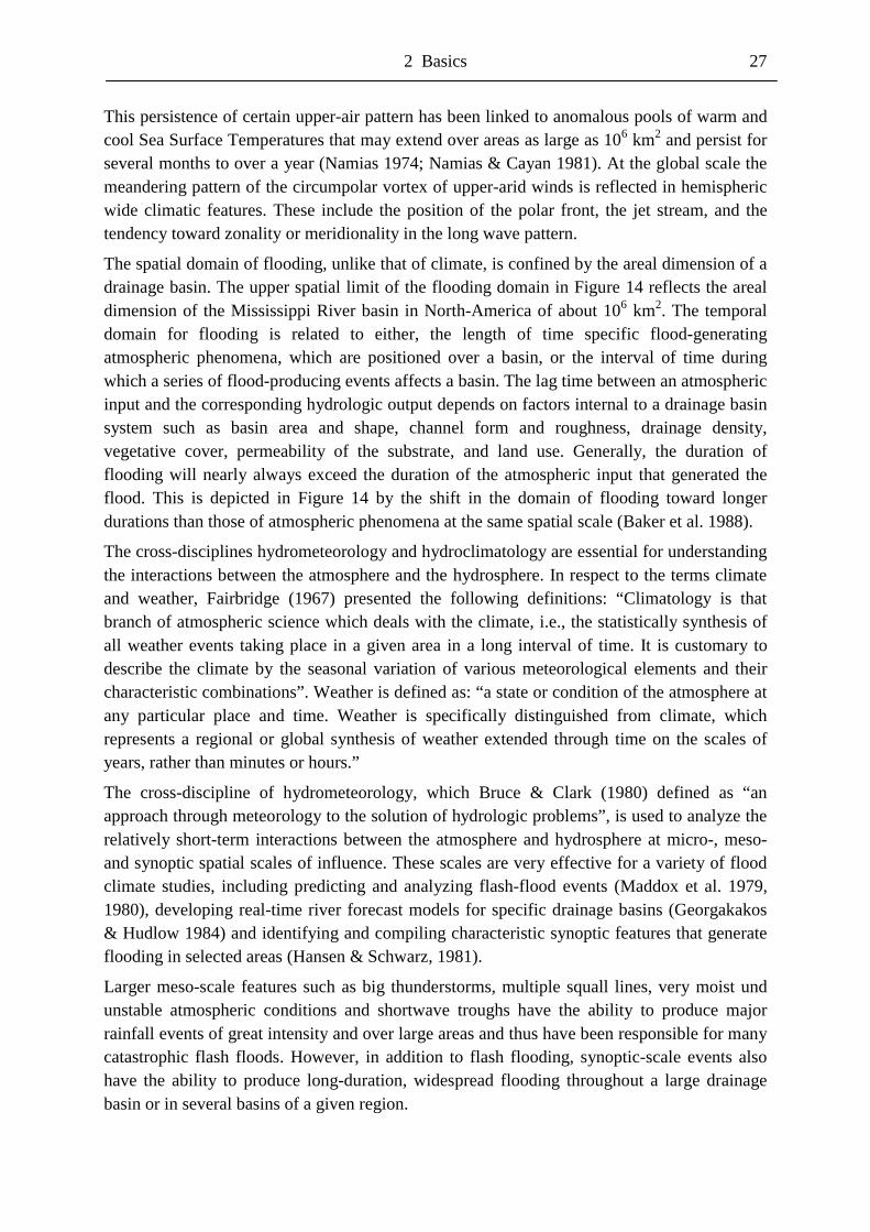
2 Basics 27

This persistence of certain upper-air pattern has been linked to anomalous pools of warm and cool Sea Surface Temperatures that may extend over areas as large as 106 km2 and persist for several months to over a year (Namias 1974; Namias & Cayan 1981). At the global scale the meandering pattern of the circumpolar vortex of upper-arid winds is reflected in hemispheric wide climatic features. These include the position of the polar front, the jet stream, and the tendency toward zonality or meridionality in the long wave pattern.

The spatial domain of flooding, unlike that of climate, is confined by the areal dimension of a drainage basin. The upper spatial limit of the flooding domain in Figure 14 reflects the areal dimension of the Mississippi River basin in North-America of about 106 km2. The temporal domain for flooding is related to either, the length of time specific flood-generating atmospheric phenomena, which are positioned over a basin, or the interval of time during which a series of flood-producing events affects a basin. The lag time between an atmospheric input and the corresponding hydrologic output depends on factors internal to a drainage basin system such as basin area and shape, channel form and roughness, drainage density, vegetative cover, permeability of the substrate, and land use. Generally, the duration of flooding will nearly always exceed the duration of the atmospheric input that generated the flood. This is depicted in Figure 14 by the shift in the domain of flooding toward longer durations than those of atmospheric phenomena at the same spatial scale (Baker et al. 1988).

The cross-disciplines hydrometeorology and hydroclimatology are essential for understanding the interactions between the atmosphere and the hydrosphere. In respect to the terms climate and weather, Fairbridge (1967) presented the following definitions: “Climatology is that branch of atmospheric science which deals with the climate, i.e., the statistically synthesis of all weather events taking place in a given area in a long interval of time. It is customary to describe the climate by the seasonal variation of various meteorological elements and their characteristic combinations”. Weather is defined as: “a state or condition of the atmosphere at any particular place and time. Weather is specifically distinguished from climate, which represents a regional or global synthesis of weather extended through time on the scales of years, rather than minutes or hours.”

The cross-discipline of hydrometeorology, which Bruce & Clark (1980) defined as “an approach through meteorology to the solution of hydrologic problems”, is used to analyze the relatively short-term interactions between the atmosphere and hydrosphere at micro-, meso- and synoptic spatial scales of influence. These scales are very effective for a variety of flood climate studies, including predicting and analyzing flash-flood events (Maddox et al. 1979, 1980), developing real-time river forecast models for specific drainage basins (Georgakakos & Hudlow 1984) and identifying and compiling characteristic synoptic features that generate flooding in selected areas (Hansen & Schwarz, 1981).

Larger meso-scale features such as big thunderstorms, multiple squall lines, very moist und unstable atmospheric conditions and shortwave troughs have the ability to produce major rainfall events of great intensity and over large areas and thus have been responsible for many catastrophic flash floods. However, in addition to flash flooding, synoptic-scale events also have the ability to produce long-duration, widespread flooding throughout a large drainage basin or in several basins of a given region.

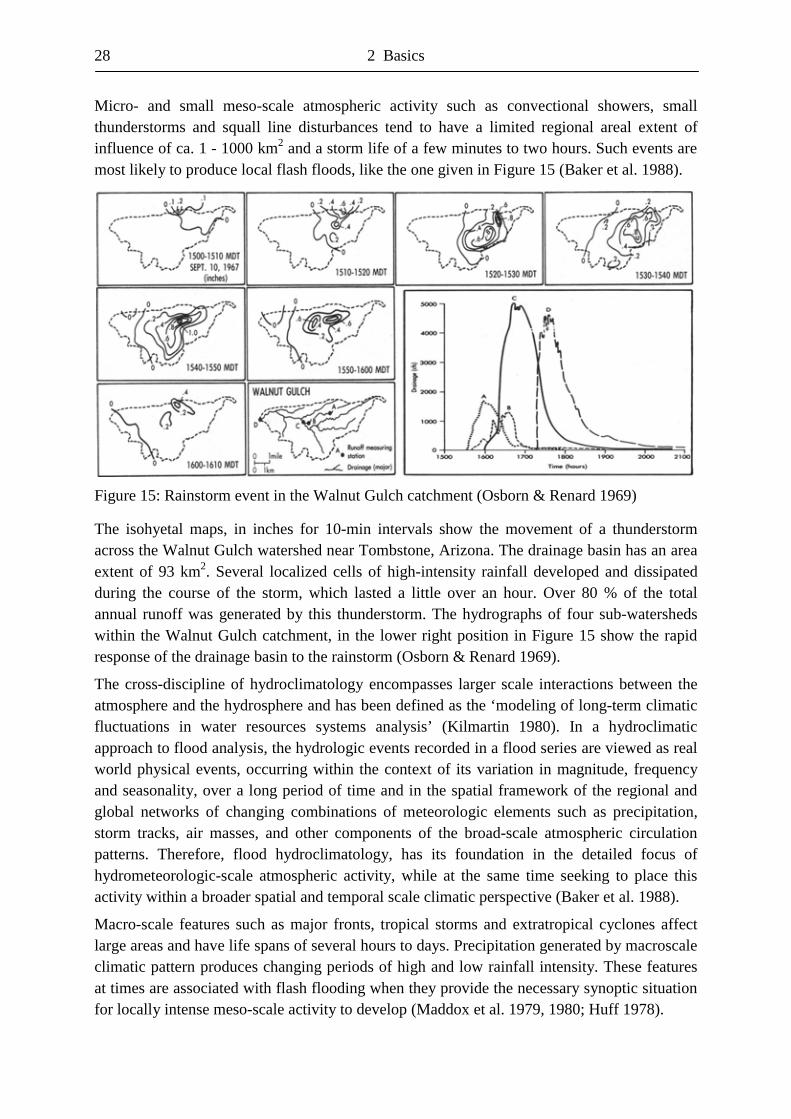
28 2 Basics

Micro- and small meso-scale atmospheric activity such as convectional showers, small thunderstorms and squall line disturbances tend to have a limited regional areal extent of influence of ca. 1 - 1000 km2 and a storm life of a few minutes to two hours. Such events are most likely to produce local flash floods, like the one given in Figure 15 (Baker et al. 1988).

Figure 15: Rainstorm event in the Walnut Gulch catchment (Osborn & Renard 1969)

The isohyetal maps, in inches for 10-min intervals show the movement of a thunderstorm across the Walnut Gulch watershed near Tombstone, Arizona. The drainage basin has an area extent of 93 km2. Several localized cells of high-intensity rainfall developed and dissipated during the course of the storm, which lasted a little over an hour. Over 80 % of the total annual runoff was generated by this thunderstorm. The hydrographs of four sub-watersheds within the Walnut Gulch catchment, in the lower right position in Figure 15 show the rapid response of the drainage basin to the rainstorm (Osborn & Renard 1969).

The cross-discipline of hydroclimatology encompasses larger scale interactions between the atmosphere and the hydrosphere and has been defined as the ‘modeling of long-term climatic fluctuations in water resources systems analysis’ (Kilmartin 1980). In a hydroclimatic approach to flood analysis, the hydrologic events recorded in a flood series are viewed as real world physical events, occurring within the context of its variation in magnitude, frequency and seasonality, over a long period of time and in the spatial framework of the regional and global networks of changing combinations of meteorologic elements such as precipitation, storm tracks, air masses, and other components of the broad-scale atmospheric circulation patterns. Therefore, flood hydroclimatology, has its foundation in the detailed focus of hydrometeorologic-scale atmospheric activity, while at the same time seeking to place this activity within a broader spatial and temporal scale climatic perspective (Baker et al. 1988).

Macro-scale features such as major fronts, tropical storms and extratropical cyclones affect large areas and have life spans of several hours to days. Precipitation generated by macroscale climatic pattern produces changing periods of high and low rainfall intensity. These features at times are associated with flash flooding when they provide the necessary synoptic situation for locally intense meso-scale activity to develop (Maddox et al. 1979, 1980; Huff 1978).

2 Basics 29

The widespread nature of these storms, coupled with their complex intensity-duration properties generally produce slow rising flood hydrographs, characterized by relatively long lasting flood water level. However, large scale and longer duration climatic events, such as snow-melting processes, anomalous configurations in the upper-level circulation, sea surface temperature anomalies and decadal-scale circulation episodes can also influence flood events. More detailed knowledge about the relationship between floods and climatic activity at larger scales is needed to identify widespread flood-generating hydrometeorologic activity being likely to develop floods. Large-scale anomaly patterns, global-scale controls and long-term trends might be overlooked in the analysis of floods limited to the hydrometeorologic space-time domain, whereas these same patterns, controls and relationships can be detected at the broader hydroclimatic domains of analysis (Baker et al. 1988).

In many cases floods result from excessive amounts of precipitation or snowmelt or from typical hydrometeorologic circulation mechanism, such as fronts, squall lines, mesoscale convective complexes or synoptic-scale cyclones, but floods can also be associated with atypical atmospheric circulation patterns. These anomalies can be in the form of an unusual combination of several common mechanisms occurring together, an unusual location or unseasonal occurrence of an otherwise typical circulation mechanism, the unusual persistence of a specific circulation pattern, or a rare configuration in the upper-air pattern itself.

According to Namias (1973), the anomaly that led to the June 1972 circulation anomaly associated with hurricane Agnes, began to establish as early as February or March, partly due to abnormally warm Sea Surface Temperature in the Atlantic, influencing the interaction between the ocean and the atmosphere. Such air-sea interactions form the basis for many long-range forecasting techniques and are argument for possible long-term, large-scale hydroclimatic controls on major flooding around the world. El Niño, the anomalous warming of Sea Surface Temperature from coastal Peru westward along the equator, and the Southern Oscillation, a related atmospheric pressure shift in the western South Pacific ocean, are the most frequently cited large-scale Sea Surface Temperature factors to be linked to flood events in regions such as Peru, Bolivia and Ecuador in South America, the Pacific coast of North America and coastal areas of the Gulf of Mexico (Quiroz 1983; Rasmusson 1985). However, in other parts of the world, the El Niño has been associated with the occurrence of droughts.

Episodic tendencies in the overall pattern of the circumpolar upper-air waves constitute the largest spatial and longest temporal scales to have a potential hydroclimatic impact on flooding. Although the ridges and troughs that form the upper-air wave pattern may adjust into high- and low-amplitude patterns on a daily, weekly, monthly or seasonal basis, over the last 100 years extended intervals of time characterized by more zonal circulation patterns have alternated with periods characterized by more meridional patterns. Theses circulation episodes often persist over several decades and have been documented in a variety of ways by researchers who have used both subjective and objective means to classify large-scale patterns and adjustments in the atmosphere over time. Circulation adjustments at these decadal scales have their greatest hydroclimatic impact in generating trends and variations in flood series over time (Dzerdzeevskii 1963, 1969; Kutzbach 1970; Kalnicky 1974; Knox et al. 1975; Lamb 1977; Barry & Perry 1973). The complete spectrum of atmospheric activity depicted in Figure 14 has the potential to generate floods, either directly or indirectly (Baker et al. 1988).

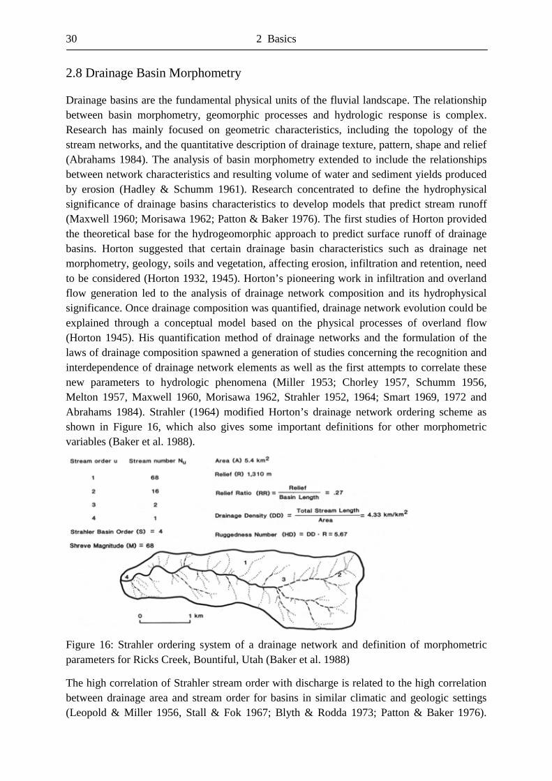
30 2 Basics

2.8 Drainage Basin Morphometry

Drainage basins are the fundamental physical units of the fluvial landscape. The relationship between basin morphometry, geomorphic processes and hydrologic response is complex. Research has mainly focused on geometric characteristics, including the topology of the stream networks, and the quantitative description of drainage texture, pattern, shape and relief (Abrahams 1984). The analysis of basin morphometry extended to include the relationships between network characteristics and resulting volume of water and sediment yields produced by erosion (Hadley & Schumm 1961). Research concentrated to define the hydrophysical significance of drainage basins characteristics to develop models that predict stream runoff (Maxwell 1960; Morisawa 1962; Patton & Baker 1976). The first studies of Horton provided the theoretical base for the hydrogeomorphic approach to predict surface runoff of drainage basins. Horton suggested that certain drainage basin characteristics such as drainage net morphometry, geology, soils and vegetation, affecting erosion, infiltration and retention, need to be considered (Horton 1932, 1945). Horton’s pioneering work in infiltration and overland flow generation led to the analysis of drainage network composition and its hydrophysical significance. Once drainage composition was quantified, drainage network evolution could be explained through a conceptual model based on the physical processes of overland flow (Horton 1945). His quantification method of drainage networks and the formulation of the laws of drainage composition spawned a generation of studies concerning the recognition and interdependence of drainage network elements as well as the first attempts to correlate these new parameters to hydrologic phenomena (Miller 1953; Chorley 1957, Schumm 1956, Melton 1957, Maxwell 1960, Morisawa 1962, Strahler 1952, 1964; Smart 1969, 1972 and Abrahams 1984). Strahler (1964) modified Horton’s drainage network ordering scheme as shown in Figure 16, which also gives some important definitions for other morphometric variables (Baker et al. 1988).

Figure 16: Strahler ordering system of a drainage network and definition of morphometric parameters for Ricks Creek, Bountiful, Utah (Baker et al. 1988)

The high correlation of Strahler stream order with discharge is related to the high correlation between drainage area and stream order for basins in similar climatic and geologic settings (Leopold & Miller 1956, Stall & Fok 1967; Blyth & Rodda 1973; Patton & Baker 1976).

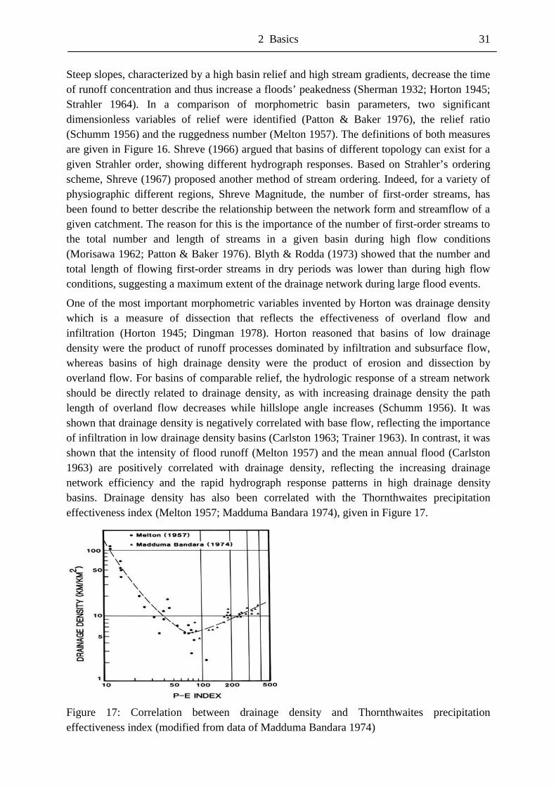
2 Basics 31

Steep slopes, characterized by a high basin relief and high stream gradients, decrease the time of runoff concentration and thus increase a floods’ peakedness (Sherman 1932; Horton 1945; Strahler 1964). In a comparison of morphometric basin parameters, two significant dimensionless variables of relief were identified (Patton & Baker 1976), the relief ratio (Schumm 1956) and the ruggedness number (Melton 1957). The definitions of both measures are given in Figure 16. Shreve (1966) argued that basins of different topology can exist for a given Strahler order, showing different hydrograph responses. Based on Strahler’s ordering scheme, Shreve (1967) proposed another method of stream ordering. Indeed, for a variety of physiographic different regions, Shreve Magnitude, the number of first-order streams, has been found to better describe the relationship between the network form and streamflow of a given catchment. The reason for this is the importance of the number of first-order streams to the total number and length of streams in a given basin during high flow conditions (Morisawa 1962; Patton & Baker 1976). Blyth & Rodda (1973) showed that the number and total length of flowing first-order streams in dry periods was lower than during high flow conditions, suggesting a maximum extent of the drainage network during large flood events.

One of the most important morphometric variables invented by Horton was drainage density which is a measure of dissection that reflects the effectiveness of overland flow and infiltration (Horton 1945; Dingman 1978). Horton reasoned that basins of low drainage density were the product of runoff processes dominated by infiltration and subsurface flow, whereas basins of high drainage density were the product of erosion and dissection by overland flow. For basins of comparable relief, the hydrologic response of a stream network should be directly related to drainage density, as with increasing drainage density the path length of overland flow decreases while hillslope angle increases (Schumm 1956). It was shown that drainage density is negatively correlated with base flow, reflecting the importance of infiltration in low drainage density basins (Carlston 1963; Trainer 1963). In contrast, it was shown that the intensity of flood runoff (Melton 1957) and the mean annual flood (Carlston 1963) are positively correlated with drainage density, reflecting the increasing drainage network efficiency and the rapid hydrograph response patterns in high drainage density basins. Drainage density has also been correlated with the Thornthwaites precipitation effectiveness index (Melton 1957; Madduma Bandara 1974), given in Figure 17.

Figure 17: Correlation between drainage density and Thornthwaites precipitation effectiveness index (modified from data of Madduma Bandara 1974)

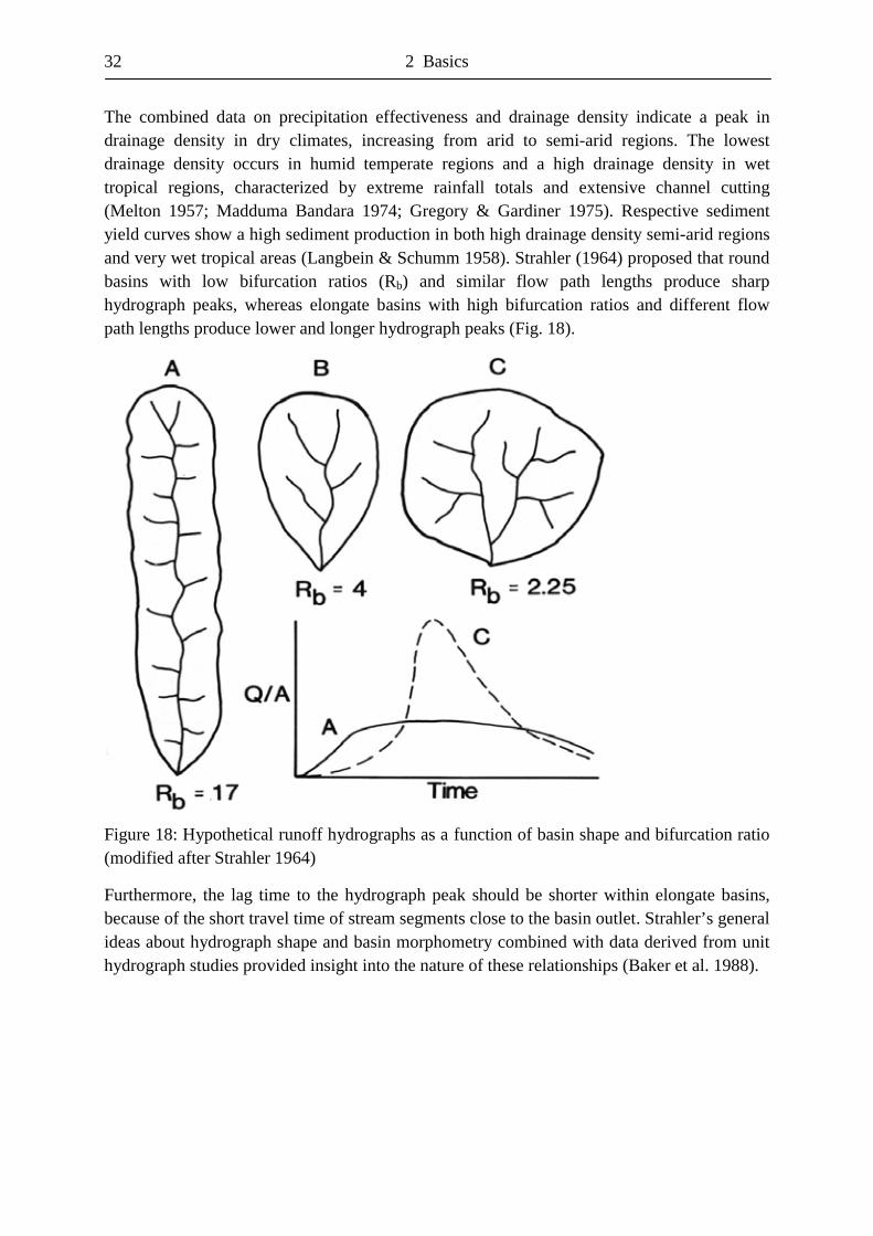
32 2 Basics

The combined data on precipitation effectiveness and drainage density indicate a peak in drainage density in dry climates, increasing from arid to semi-arid regions. The lowest drainage density occurs in humid temperate regions and a high drainage density in wet tropical regions, characterized by extreme rainfall totals and extensive channel cutting (Melton 1957; Madduma Bandara 1974; Gregory & Gardiner 1975). Respective sediment yield curves show a high sediment production in both high drainage density semi-arid regions and very wet tropical areas (Langbein & Schumm 1958). Strahler (1964) proposed that round basins with low bifurcation ratios (Rb) and similar flow path lengths produce sharp hydrograph peaks, whereas elongate basins with high bifurcation ratios and different flow path lengths produce lower and longer hydrograph peaks (Fig. 18).

Figure 18: Hypothetical runoff hydrographs as a function of basin shape and bifurcation ratio (modified after Strahler 1964)

Furthermore, the lag time to the hydrograph peak should be shorter within elongate basins, because of the short travel time of stream segments close to the basin outlet. Strahler’s general ideas about hydrograph shape and basin morphometry combined with data derived from unit hydrograph studies provided insight into the nature of these relationships (Baker et al. 1988).

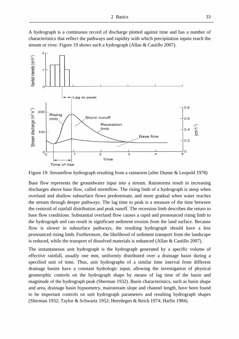
2 Basics 33

A hydrograph is a continuous record of discharge plotted against time and has a number of characteristics that reflect the pathways and rapidity with which precipitation inputs reach the stream or river. Figure 19 shows such a hydrograph (Allan & Castillo 2007).

Figure 19: Streamflow hydrograph resulting from a rainstorm (after Dunne & Leopold 1978)

Base flow represents the groundwater input into a stream. Rainstorms result in increasing discharges above base flow, called stormflow. The rising limb of a hydrograph is steep when overland and shallow subsurface flows predominate, and more gradual when water reaches the stream through deeper pathways. The lag time to peak is a measure of the time between the centroid of rainfall distribution and peak runoff. The recession limb describes the return to base flow conditions. Substantial overland flow causes a rapid and pronounced rising limb to the hydrograph and can result in significant sediment erosion from the land surface. Because flow is slower in subsurface pathways, the resulting hydrograph should have a less pronounced rising limb. Furthermore, the likelihood of sediment transport from the landscape is reduced, while the transport of dissolved materials is enhanced (Allan & Castillo 2007).

The instantaneous unit hydrograph is the hydrograph generated by a specific volume of effective rainfall, usually one mm, uniformly distributed over a drainage basin during a specified unit of time. Thus, unit hydrographs of a similar time interval from different drainage basins have a constant hydrologic input, allowing the investigation of physical geomorphic controls on the hydrograph shape by means of lag time of the basin and magnitude of the hydrograph peak (Sherman 1932). Basin characteristics, such as basin shape and area, drainage basin hypsometry, mainstream slope and channel length, have been found to be important controls on unit hydrograph parameters and resulting hydrograph shapes (Sherman 1932; Taylor & Schwartz 1952; Heerdegen & Reich 1974; Harlin 1984).

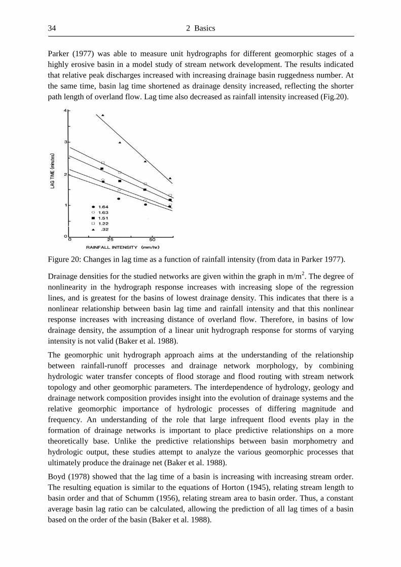
34 2 Basics

Parker (1977) was able to measure unit hydrographs for different geomorphic stages of a highly erosive basin in a model study of stream network development. The results indicated that relative peak discharges increased with increasing drainage basin ruggedness number. At the same time, basin lag time shortened as drainage density increased, reflecting the shorter path length of overland flow. Lag time also decreased as rainfall intensity increased (Fig.20).

Figure 20: Changes in lag time as a function of rainfall intensity (from data in Parker 1977).

Drainage densities for the studied networks are given within the graph in m/m2. The degree of nonlinearity in the hydrograph response increases with increasing slope of the regression lines, and is greatest for the basins of lowest drainage density. This indicates that there is a nonlinear relationship between basin lag time and rainfall intensity and that this nonlinear response increases with increasing distance of overland flow. Therefore, in basins of low drainage density, the assumption of a linear unit hydrograph response for storms of varying intensity is not valid (Baker et al. 1988).

The geomorphic unit hydrograph approach aims at the understanding of the relationship between rainfall-runoff processes and drainage network morphology, by combining hydrologic water transfer concepts of flood storage and flood routing with stream network topology and other geomorphic parameters. The interdependence of hydrology, geology and drainage network composition provides insight into the evolution of drainage systems and the relative geomorphic importance of hydrologic processes of differing magnitude and frequency. An understanding of the role that large infrequent flood events play in the formation of drainage networks is important to place predictive relationships on a more theoretically base. Unlike the predictive relationships between basin morphometry and hydrologic output, these studies attempt to analyze the various geomorphic processes that ultimately produce the drainage net (Baker et al. 1988).

Boyd (1978) showed that the lag time of a basin is increasing with increasing stream order. The resulting equation is similar to the equations of Horton (1945), relating stream length to basin order and that of Schumm (1956), relating stream area to basin order. Thus, a constant average basin lag ratio can be calculated, allowing the prediction of all lag times of a basin based on the order of the basin (Baker et al. 1988).

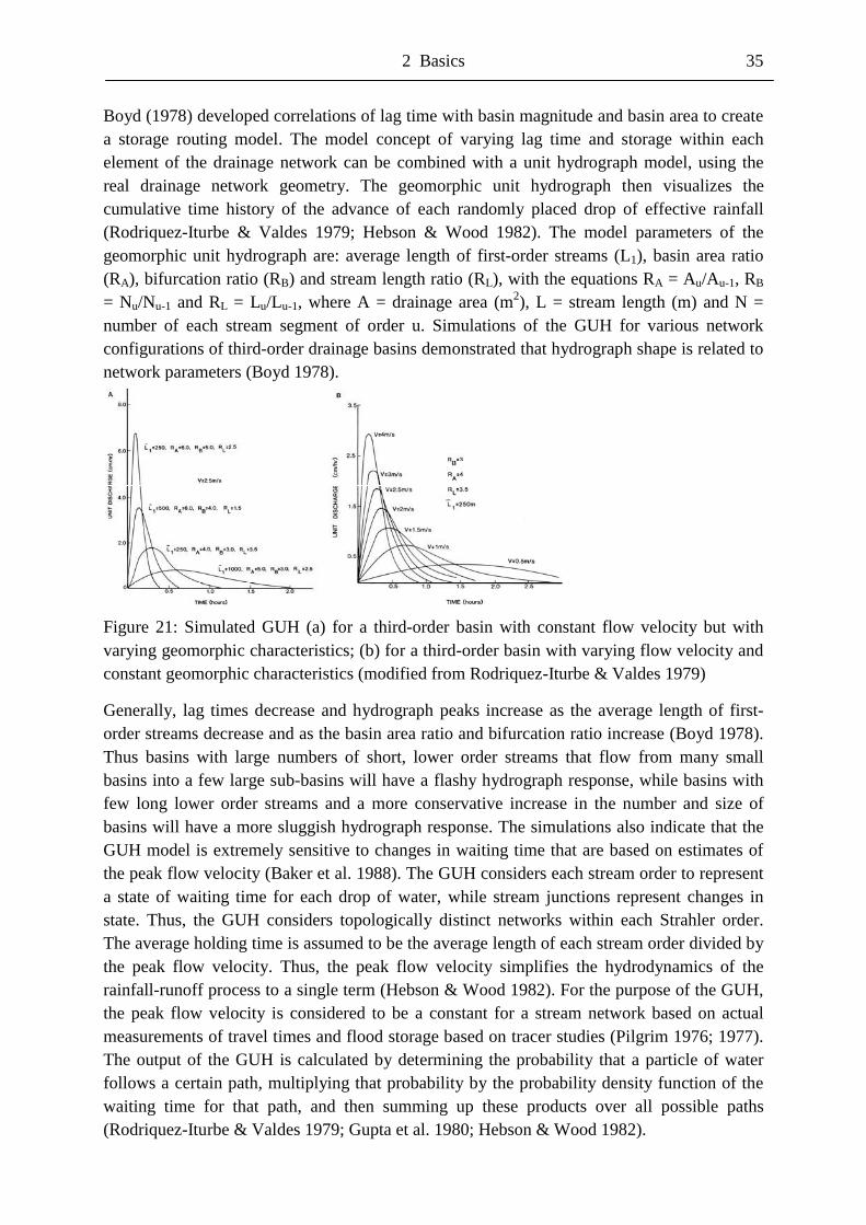
2 Basics 35

Boyd (1978) developed correlations of lag time with basin magnitude and basin area to create a storage routing model. The model concept of varying lag time and storage within each element of the drainage network can be combined with a unit hydrograph model, using the real drainage network geometry. The geomorphic unit hydrograph then visualizes the cumulative time history of the advance of each randomly placed drop of effective rainfall (Rodriquez-Iturbe & Valdes 1979; Hebson & Wood 1982). The model parameters of the geomorphic unit hydrograph are: average length of first-order streams (L1), basin area ratio (RA), bifurcation ratio (RB) and stream length ratio (RL), with the equations RA = Au/Au-1, RB = Nu/Nu-1 and RL = Lu/Lu-1, where A = drainage area (m2), L = stream length (m) and N = number of each stream segment of order u. Simulations of the GUH for various network configurations of third-order drainage basins demonstrated that hydrograph shape is related to network parameters (Boyd 1978).

Figure 21: Simulated GUH (a) for a third-order basin with constant flow velocity but with varying geomorphic characteristics; (b) for a third-order basin with varying flow velocity and constant geomorphic characteristics (modified from Rodriquez-Iturbe & Valdes 1979)

Generally, lag times decrease and hydrograph peaks increase as the average length of first-order streams decrease and as the basin area ratio and bifurcation ratio increase (Boyd 1978). Thus basins with large numbers of short, lower order streams that flow from many small basins into a few large sub-basins will have a flashy hydrograph response, while basins with few long lower order streams and a more conservative increase in the number and size of basins will have a more sluggish hydrograph response. The simulations also indicate that the GUH model is extremely sensitive to changes in waiting time that are based on estimates of the peak flow velocity (Baker et al. 1988). The GUH considers each stream order to represent a state of waiting time for each drop of water, while stream junctions represent changes in state. Thus, the GUH considers topologically distinct networks within each Strahler order. The average holding time is assumed to be the average length of each stream order divided by the peak flow velocity. Thus, the peak flow velocity simplifies the hydrodynamics of the rainfall-runoff process to a single term (Hebson & Wood 1982). For the purpose of the GUH, the peak flow velocity is considered to be a constant for a stream network based on actual measurements of travel times and flood storage based on tracer studies (Pilgrim 1976; 1977). The output of the GUH is calculated by determining the probability that a particle of water follows a certain path, multiplying that probability by the probability density function of the waiting time for that path, and then summing up these products over all possible paths (Rodriquez-Iturbe & Valdes 1979; Gupta et al. 1980; Hebson & Wood 1982).

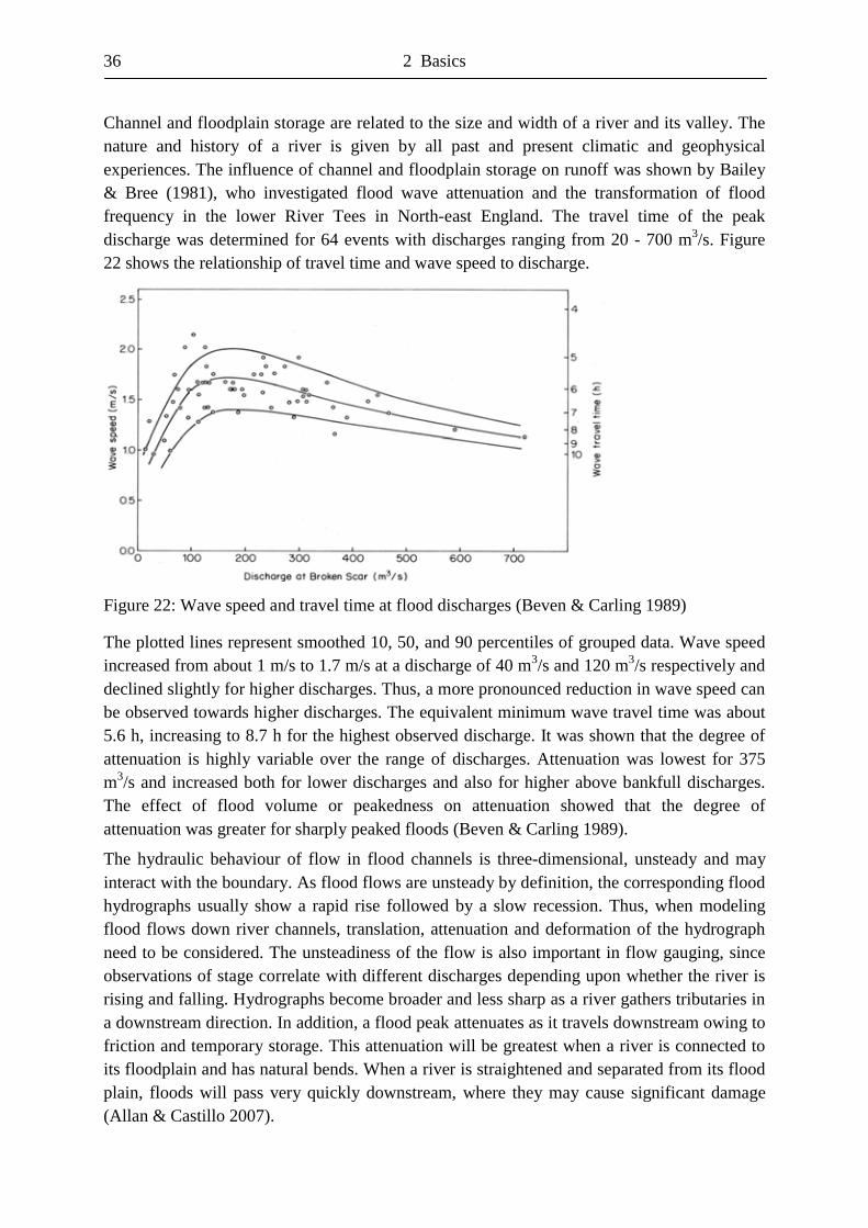
36 2 Basics

Channel and floodplain storage are related to the size and width of a river and its valley. The nature and history of a river is given by all past and present climatic and geophysical experiences. The influence of channel and floodplain storage on runoff was shown by Bailey & Bree (1981), who investigated flood wave attenuation and the transformation of flood frequency in the lower River Tees in North-east England. The travel time of the peak discharge was determined for 64 events with discharges ranging from 20 - 700 m3/s. Figure 22 shows the relationship of travel time and wave speed to discharge.

Figure 22: Wave speed and travel time at flood discharges (Beven & Carling 1989)

The plotted lines represent smoothed 10, 50, and 90 percentiles of grouped data. Wave speed increased from about 1 m/s to 1.7 m/s at a discharge of 40 m3/s and 120 m3/s respectively and declined slightly for higher discharges. Thus, a more pronounced reduction in wave speed can be observed towards higher discharges. The equivalent minimum wave travel time was about 5.6 h, increasing to 8.7 h for the highest observed discharge. It was shown that the degree of attenuation is highly variable over the range of discharges. Attenuation was lowest for 375 m3/s and increased both for lower discharges and also for higher above bankfull discharges. The effect of flood volume or peakedness on attenuation showed that the degree of attenuation was greater for sharply peaked floods (Beven & Carling 1989).

The hydraulic behaviour of flow in flood channels is three-dimensional, unsteady and may interact with the boundary. As flood flows are unsteady by definition, the corresponding flood hydrographs usually show a rapid rise followed by a slow recession. Thus, when modeling flood flows down river channels, translation, attenuation and deformation of the hydrograph need to be considered. The unsteadiness of the flow is also important in flow gauging, since observations of stage correlate with different discharges depending upon whether the river is rising and falling. Hydrographs become broader and less sharp as a river gathers tributaries in a downstream direction. In addition, a flood peak attenuates as it travels downstream owing to friction and temporary storage. This attenuation will be greatest when a river is connected to its floodplain and has natural bends. When a river is straightened and separated from its flood plain, floods will pass very quickly downstream, where they may cause significant damage (Allan & Castillo 2007).

2 Basics 37

Velocity:

The velocity in a stream varies in space and time. Mean velocity across any section is:

AQV = [m/s] (1)

where Q = discharge (m3/s) and A = cross-sectional area (m2). Flow velocity tends to increase as the slope increases and as bed roughness decreases (Gordon et al. 2004).

Flow in open channels can be classified in four ways: steady or unsteady, uniform or varied, laminar or turbulent and supercritical, critical or subcritical.

The first classification of steady or unsteady depends on whether the flow depth and velocity at a particular point change with time. In contrast, the classification of uniform or varied depends on whether flow depth and velocity vary with respect to distance. If depth and velocity remain constant over some length of a channel of constant cross-section and slope, then the water surface is parallel to the streambed and flow is uniform and moving at its ‘normal depth’. The assumption of uniform flow conditions simplifies the analysis of water movement in streams. If the flow in a stream is non-uniform or varied, the water depth and/or velocity change over distance. Varied flow can be sub-divided further into the categories rapidly varied and gradually varied. If the depth changes abruptly over a relatively short distance, as at a waterfall or wave, the flow is rapidly varied, and if changes are more widely spread, the flow is gradually varied. Uniform flow can be approximated by long, straight runs of constant slope and cross-section. The third classification of laminar or turbulent is irrelevant at the ‘macro-environment’ level. Although regions of laminar flow can exist near the surfaces of rocks or organisms within the stream, the bulk flow is nearly always turbulent except perhaps in the rare case where it flows slowly as a thin film of a few millimetres. The fourth classification of supercritical, critical or subcritical is related to the combined patterns of velocity and depth.

For a complete description of velocity distributions in streams, the concept of spiral, helical or secondary flow should be mentioned. Spiral flow is a consequence of frictional resistance and centrifugal force. When a cup of billy tea is stirred this is the reason why the leaves congregate in the middle rather than at the edges. In a stream, water is hurled against the outside banks at bends, causing the water surface to be ‘super-elevated’. The increase in elevation creates a gradient causing flow movement from the outer to the inner bank. A spiralling motion is generated along the general direction of flow (Petts & Foster 1985). Compared to the forward, downstream currents, secondary lateral and vertical currents are relatively small, yet they cause the mainstream current to vary from a predictable course and contribute to energy losses and bank erosion at bends. On the outside of a bend the rotary flow motion is downward, thereby scouring the bank. On the inside of a bend the flow is upward and decelerating, and any material carried tends to deposit, creating point bars (Vennard & Street 1982). Spiral flow also occurs in straight sections, where the welling of waters near the stream’s centre can increase the local surface elevation, resulting in a curved water surface (Leopold et al. 1964). Spiral flow is particularly pronounced where channel boundaries are irregular. (Gordon et al. 2004).

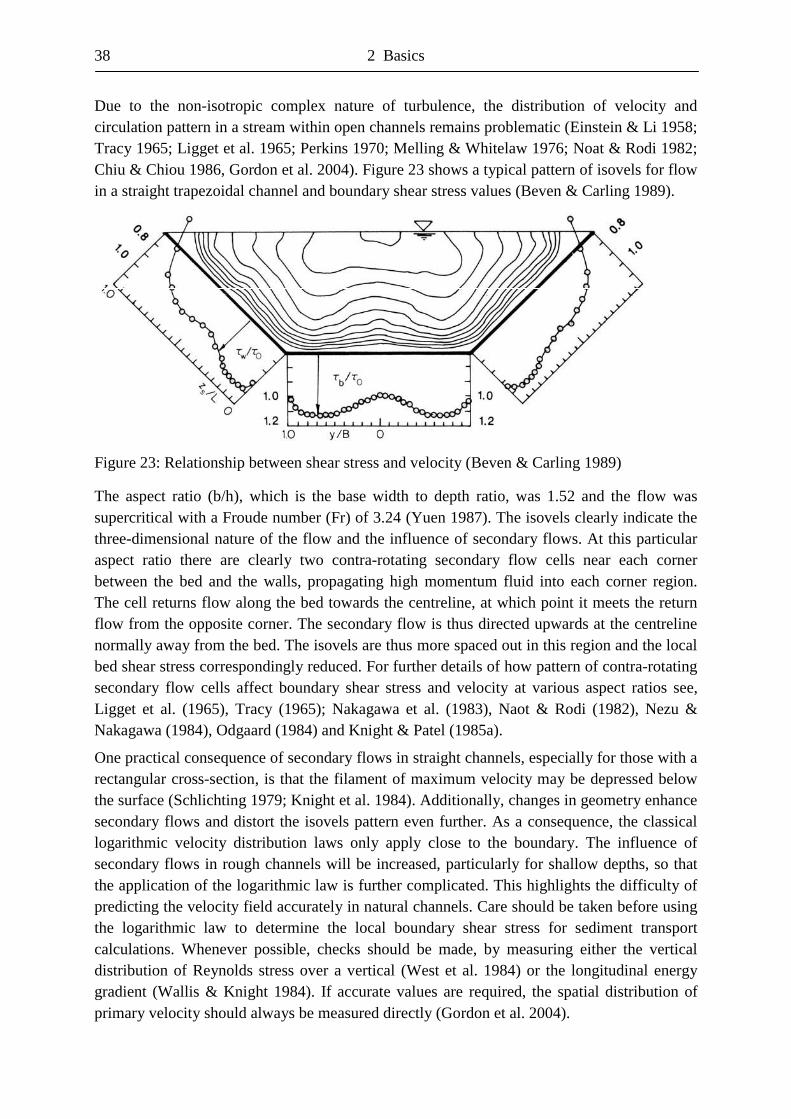
38 2 Basics

Due to the non-isotropic complex nature of turbulence, the distribution of velocity and circulation pattern in a stream within open channels remains problematic (Einstein & Li 1958; Tracy 1965; Ligget et al. 1965; Perkins 1970; Melling & Whitelaw 1976; Noat & Rodi 1982; Chiu & Chiou 1986, Gordon et al. 2004). Figure 23 shows a typical pattern of isovels for flow in a straight trapezoidal channel and boundary shear stress values (Beven & Carling 1989).

Figure 23: Relationship between shear stress and velocity (Beven & Carling 1989)

The aspect ratio (b/h), which is the base width to depth ratio, was 1.52 and the flow was supercritical with a Froude number (Fr) of 3.24 (Yuen 1987). The isovels clearly indicate the three-dimensional nature of the flow and the influence of secondary flows. At this particular aspect ratio there are clearly two contra-rotating secondary flow cells near each corner between the bed and the walls, propagating high momentum fluid into each corner region. The cell returns flow along the bed towards the centreline, at which point it meets the return flow from the opposite corner. The secondary flow is thus directed upwards at the centreline normally away from the bed. The isovels are thus more spaced out in this region and the local bed shear stress correspondingly reduced. For further details of how pattern of contra-rotating secondary flow cells affect boundary shear stress and velocity at various aspect ratios see, Ligget et al. (1965), Tracy (1965); Nakagawa et al. (1983), Naot & Rodi (1982), Nezu & Nakagawa (1984), Odgaard (1984) and Knight & Patel (1985a).

One practical consequence of secondary flows in straight channels, especially for those with a rectangular cross-section, is that the filament of maximum velocity may be depressed below the surface (Schlichting 1979; Knight et al. 1984). Additionally, changes in geometry enhance secondary flows and distort the isovels pattern even further. As a consequence, the classical logarithmic velocity distribution laws only apply close to the boundary. The influence of secondary flows in rough channels will be increased, particularly for shallow depths, so that the application of the logarithmic law is further complicated. This highlights the difficulty of predicting the velocity field accurately in natural channels. Care should be taken before using the logarithmic law to determine the local boundary shear stress for sediment transport calculations. Whenever possible, checks should be made, by measuring either the vertical distribution of Reynolds stress over a vertical (West et al. 1984) or the longitudinal energy gradient (Wallis & Knight 1984). If accurate values are required, the spatial distribution of primary velocity should always be measured directly (Gordon et al. 2004).

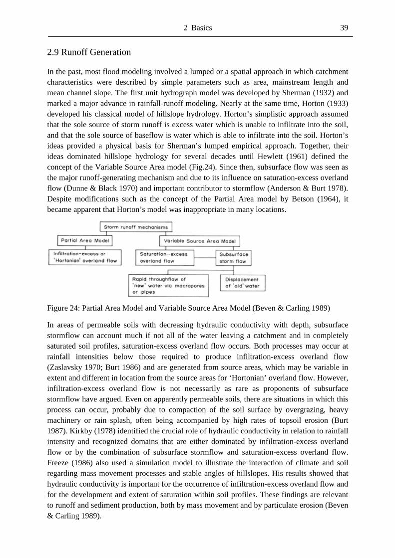
2 Basics 39

2.9 Runoff Generation

In the past, most flood modeling involved a lumped or a spatial approach in which catchment characteristics were described by simple parameters such as area, mainstream length and mean channel slope. The first unit hydrograph model was developed by Sherman (1932) and marked a major advance in rainfall-runoff modeling. Nearly at the same time, Horton (1933) developed his classical model of hillslope hydrology. Horton’s simplistic approach assumed that the sole source of storm runoff is excess water which is unable to infiltrate into the soil, and that the sole source of baseflow is water which is able to infiltrate into the soil. Horton’s ideas provided a physical basis for Sherman’s lumped empirical approach. Together, their ideas dominated hillslope hydrology for several decades until Hewlett (1961) defined the concept of the Variable Source Area model (Fig.24). Since then, subsurface flow was seen as the major runoff-generating mechanism and due to its influence on saturation-excess overland flow (Dunne & Black 1970) and important contributor to stormflow (Anderson & Burt 1978). Despite modifications such as the concept of the Partial Area model by Betson (1964), it became apparent that Horton’s model was inappropriate in many locations.

Figure 24: Partial Area Model and Variable Source Area Model (Beven & Carling 1989)

In areas of permeable soils with decreasing hydraulic conductivity with depth, subsurface stormflow can account much if not all of the water leaving a catchment and in completely saturated soil profiles, saturation-excess overland flow occurs. Both processes may occur at rainfall intensities below those required to produce infiltration-excess overland flow (Zaslavsky 1970; Burt 1986) and are generated from source areas, which may be variable in extent and different in location from the source areas for ‘Hortonian’ overland flow. However, infiltration-excess overland flow is not necessarily as rare as proponents of subsurface stormflow have argued. Even on apparently permeable soils, there are situations in which this process can occur, probably due to compaction of the soil surface by overgrazing, heavy machinery or rain splash, often being accompanied by high rates of topsoil erosion (Burt 1987). Kirkby (1978) identified the crucial role of hydraulic conductivity in relation to rainfall intensity and recognized domains that are either dominated by infiltration-excess overland flow or by the combination of subsurface stormflow and saturation-excess overland flow. Freeze (1986) also used a simulation model to illustrate the interaction of climate and soil regarding mass movement processes and stable angles of hillslopes. His results showed that hydraulic conductivity is important for the occurrence of infiltration-excess overland flow and for the development and extent of saturation within soil profiles. These findings are relevant to runoff and sediment production, both by mass movement and by particulate erosion (Beven & Carling 1989).

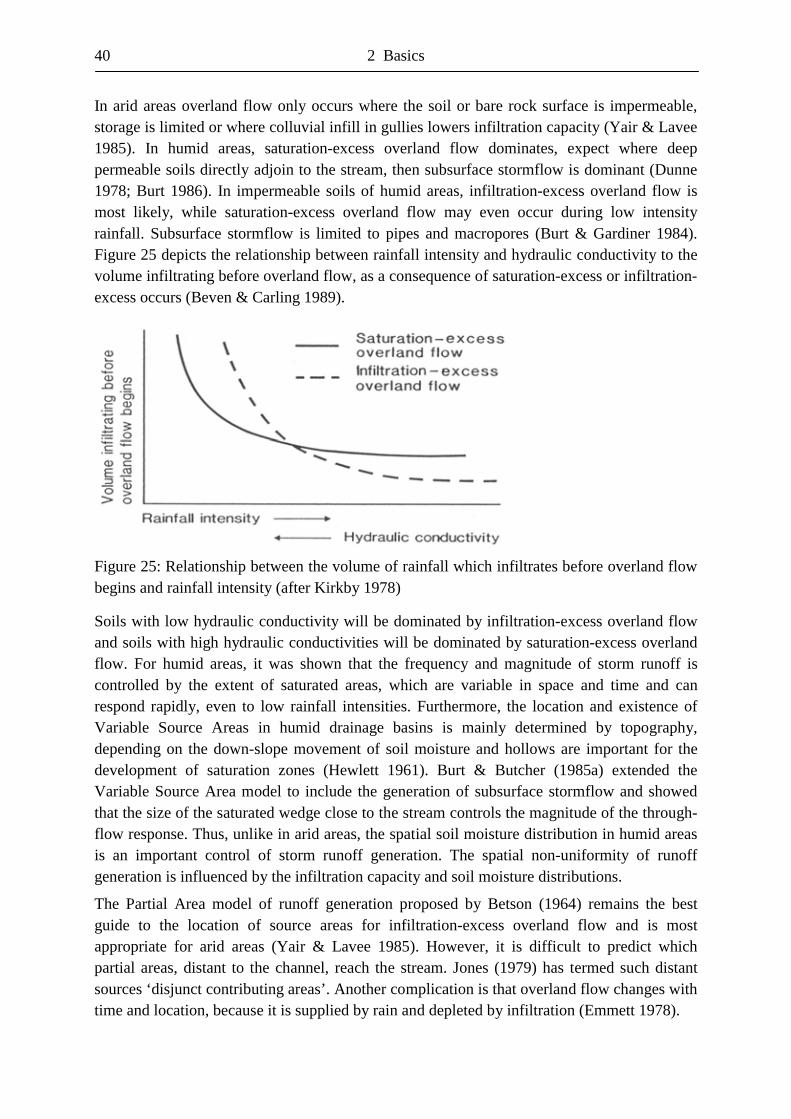
40 2 Basics

In arid areas overland flow only occurs where the soil or bare rock surface is impermeable, storage is limited or where colluvial infill in gullies lowers infiltration capacity (Yair & Lavee 1985). In humid areas, saturation-excess overland flow dominates, expect where deep permeable soils directly adjoin to the stream, then subsurface stormflow is dominant (Dunne 1978; Burt 1986). In impermeable soils of humid areas, infiltration-excess overland flow is most likely, while saturation-excess overland flow may even occur during low intensity rainfall. Subsurface stormflow is limited to pipes and macropores (Burt & Gardiner 1984). Figure 25 depicts the relationship between rainfall intensity and hydraulic conductivity to the volume infiltrating before overland flow, as a consequence of saturation-excess or infiltration-excess occurs (Beven & Carling 1989).

Figure 25: Relationship between the volume of rainfall which infiltrates before overland flow begins and rainfall intensity (after Kirkby 1978)

Soils with low hydraulic conductivity will be dominated by infiltration-excess overland flow and soils with high hydraulic conductivities will be dominated by saturation-excess overland flow. For humid areas, it was shown that the frequency and magnitude of storm runoff is controlled by the extent of saturated areas, which are variable in space and time and can respond rapidly, even to low rainfall intensities. Furthermore, the location and existence of Variable Source Areas in humid drainage basins is mainly determined by topography, depending on the down-slope movement of soil moisture and hollows are important for the development of saturation zones (Hewlett 1961). Burt & Butcher (1985a) extended the Variable Source Area model to include the generation of subsurface stormflow and showed that the size of the saturated wedge close to the stream controls the magnitude of the through-flow response. Thus, unlike in arid areas, the spatial soil moisture distribution in humid areas is an important control of storm runoff generation. The spatial non-uniformity of runoff generation is influenced by the infiltration capacity and soil moisture distributions.

The Partial Area model of runoff generation proposed by Betson (1964) remains the best guide to the location of source areas for infiltration-excess overland flow and is most appropriate for arid areas (Yair & Lavee 1985). However, it is difficult to predict which partial areas, distant to the channel, reach the stream. Jones (1979) has termed such distant sources ‘disjunct contributing areas’. Another complication is that overland flow changes with time and location, because it is supplied by rain and depleted by infiltration (Emmett 1978).

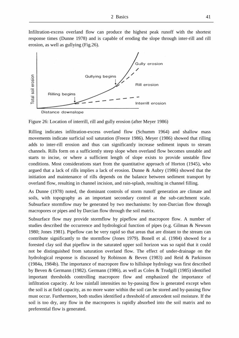
2 Basics 41

Infiltration-excess overland flow can produce the highest peak runoff with the shortest response times (Dunne 1978) and is capable of eroding the slope through inter-rill and rill erosion, as well as gullying (Fig.26).

Figure 26: Location of interrill, rill and gully erosion (after Meyer 1986)

Rilling indicates infiltration-excess overland flow (Schumm 1964) and shallow mass movements indicate surficial soil saturation (Freeze 1986). Meyer (1986) showed that rilling adds to inter-rill erosion and thus can significantly increase sediment inputs to stream channels. Rills form on a sufficiently steep slope when overland flow becomes unstable and starts to incise, or where a sufficient length of slope exists to provide unstable flow conditions. Most considerations start from the quantitative approach of Horton (1945), who argued that a lack of rills implies a lack of erosion. Dunne & Aubry (1986) showed that the initiation and maintenance of rills depends on the balance between sediment transport by overland flow, resulting in channel incision, and rain-splash, resulting in channel filling.

As Dunne (1978) noted, the dominant controls of storm runoff generation are climate and soils, with topography as an important secondary control at the sub-catchment scale. Subsurface stormflow may be generated by two mechanisms: by non-Darcian flow through macropores or pipes and by Darcian flow through the soil matrix.

Subsurface flow may provide stormflow by pipeflow and macropore flow. A number of studies described the occurrence and hydrological function of pipes (e.g. Gilman & Newson 1980; Jones 1981). Pipeflow can be very rapid so that areas that are distant to the stream can contribute significantly to the stormflow (Jones 1979). Bonell et al. (1984) showed for a forested clay soil that pipeflow in the saturated upper soil horizon was so rapid that it could not be distinguished from saturation overland flow. The effect of under-drainage on the hydrological response is discussed by Robinson & Beven (1983) and Reid & Parkinson (1984a, 1984b). The importance of macropore flow to hillslope hydrology was first described by Beven & Germann (1982). Germann (1986), as well as Coles & Trudgill (1985) identified important thresholds controlling macropore flow and emphasized the importance of infiltration capacity. At low rainfall intensities no by-passing flow is generated except when the soil is at field capacity, as no more water within the soil can be stored and by-passing flow must occur. Furthermore, both studies identified a threshold of antecedent soil moisture. If the soil is too dry, any flow in the macropores is rapidly absorbed into the soil matrix and no preferential flow is generated.

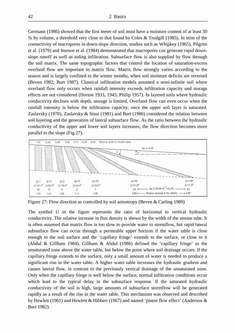
42 2 Basics

Germann (1986) showed that the first meter of soil must have a moisture content of at least 30 % by volume, a threshold very close to that found by Coles & Trudgill (1985). In term of the connectivity of macropores in down-slope direction, studies such as Whipkey (1965), Pilgrim et al. (1979) and Imeson et al. (1984) demonstrated that macropores can generate rapid down-slope runoff as well as aiding infiltration. Subsurface flow is also supplied by flow through the soil matrix. The same topographic factors that control the location of saturation-excess overland flow are important in matrix flow. Matrix flow strongly varies according to the season and is largely confined to the winter months, when soil moisture deficits are reversed (Beven 1982; Burt 1987). Classical infiltration models assumed a semi-infinite soil where overland flow only occurs when rainfall intensity exceeds infiltration capacity und storage effects are not considered (Horton 1933, 1945; Philip 1957). In layered soils where hydraulic conductivity declines with depth, storage is limited. Overland flow can even occur when the rainfall intensity is below the infiltration capacity, once the upper soil layer is saturated. Zaslavsky (1970), Zaslavsky & Sinai (1981) and Burt (1986) considered the relation between soil layering and the generation of lateral subsurface flow. As the ratio between the hydraulic conductivity of the upper and lower soil layers increases, the flow direction becomes more parallel to the slope (Fig.27).

Figure 27: Flow direction as controlled by soil anisotropy (Beven & Carling 1989)

The symbol U in the figure represents the ratio of horizontal to vertical hydraulic conductivity. The relative increase in flux density is shown by the width of the stream tube. It is often assumed that matrix flow is too slow to provide water to stormflow, but rapid lateral subsurface flow can occur through a permeable upper horizon if the water table is close enough to the soil surface and the ‘capillary fringe’ extends to the surface, or close to it (Abdul & Gillham 1984). Gillham & Abdul (1986) defined the ‘capillary fringe’ as the unsaturated zone above the water table, but below the point where soil drainage occurs. If the capillary fringe extends to the surface, only a small amount of water is needed to produce a significant rise in the water table. A higher water table increases the hydraulic gradient and causes lateral flow, in contrast to the previously vertical drainage of the unsaturated zone. Only when the capillary fringe is well below the surface, normal infiltration conditions occur which lead to the typical delay in the subsurface response. If the saturated hydraulic conductivity of the soil is high, large amounts of subsurface stormflow will be generated rapidly as a result of the rise in the water table. This mechanism was observed and described by Hewlett (1961) and Hewlett & Hibbert (1967) and named ‘piston flow effect’ (Anderson & Burt 1982).

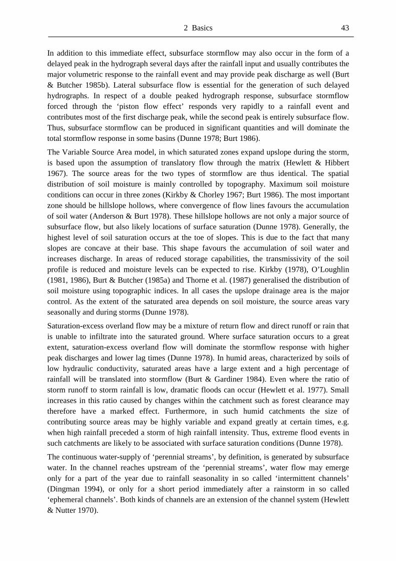
2 Basics 43

In addition to this immediate effect, subsurface stormflow may also occur in the form of a delayed peak in the hydrograph several days after the rainfall input and usually contributes the major volumetric response to the rainfall event and may provide peak discharge as well (Burt & Butcher 1985b). Lateral subsurface flow is essential for the generation of such delayed hydrographs. In respect of a double peaked hydrograph response, subsurface stormflow forced through the ‘piston flow effect’ responds very rapidly to a rainfall event and contributes most of the first discharge peak, while the second peak is entirely subsurface flow. Thus, subsurface stormflow can be produced in significant quantities and will dominate the total stormflow response in some basins (Dunne 1978; Burt 1986).

The Variable Source Area model, in which saturated zones expand upslope during the storm, is based upon the assumption of translatory flow through the matrix (Hewlett & Hibbert 1967). The source areas for the two types of stormflow are thus identical. The spatial distribution of soil moisture is mainly controlled by topography. Maximum soil moisture conditions can occur in three zones (Kirkby & Chorley 1967; Burt 1986). The most important zone should be hillslope hollows, where convergence of flow lines favours the accumulation of soil water (Anderson & Burt 1978). These hillslope hollows are not only a major source of subsurface flow, but also likely locations of surface saturation (Dunne 1978). Generally, the highest level of soil saturation occurs at the toe of slopes. This is due to the fact that many slopes are concave at their base. This shape favours the accumulation of soil water and increases discharge. In areas of reduced storage capabilities, the transmissivity of the soil profile is reduced and moisture levels can be expected to rise. Kirkby (1978), O’Loughlin (1981, 1986), Burt & Butcher (1985a) and Thorne et al. (1987) generalised the distribution of soil moisture using topographic indices. In all cases the upslope drainage area is the major control. As the extent of the saturated area depends on soil moisture, the source areas vary seasonally and during storms (Dunne 1978).

Saturation-excess overland flow may be a mixture of return flow and direct runoff or rain that is unable to infiltrate into the saturated ground. Where surface saturation occurs to a great extent, saturation-excess overland flow will dominate the stormflow response with higher peak discharges and lower lag times (Dunne 1978). In humid areas, characterized by soils of low hydraulic conductivity, saturated areas have a large extent and a high percentage of rainfall will be translated into stormflow (Burt & Gardiner 1984). Even where the ratio of storm runoff to storm rainfall is low, dramatic floods can occur (Hewlett et al. 1977). Small increases in this ratio caused by changes within the catchment such as forest clearance may therefore have a marked effect. Furthermore, in such humid catchments the size of contributing source areas may be highly variable and expand greatly at certain times, e.g. when high rainfall preceded a storm of high rainfall intensity. Thus, extreme flood events in such catchments are likely to be associated with surface saturation conditions (Dunne 1978).

The continuous water-supply of ‘perennial streams’, by definition, is generated by subsurface water. In the channel reaches upstream of the ‘perennial streams’, water flow may emerge only for a part of the year due to rainfall seasonality in so called ‘intermittent channels’ (Dingman 1994), or only for a short period immediately after a rainstorm in so called ‘ephemeral channels’. Both kinds of channels are an extension of the channel system (Hewlett & Nutter 1970).

44

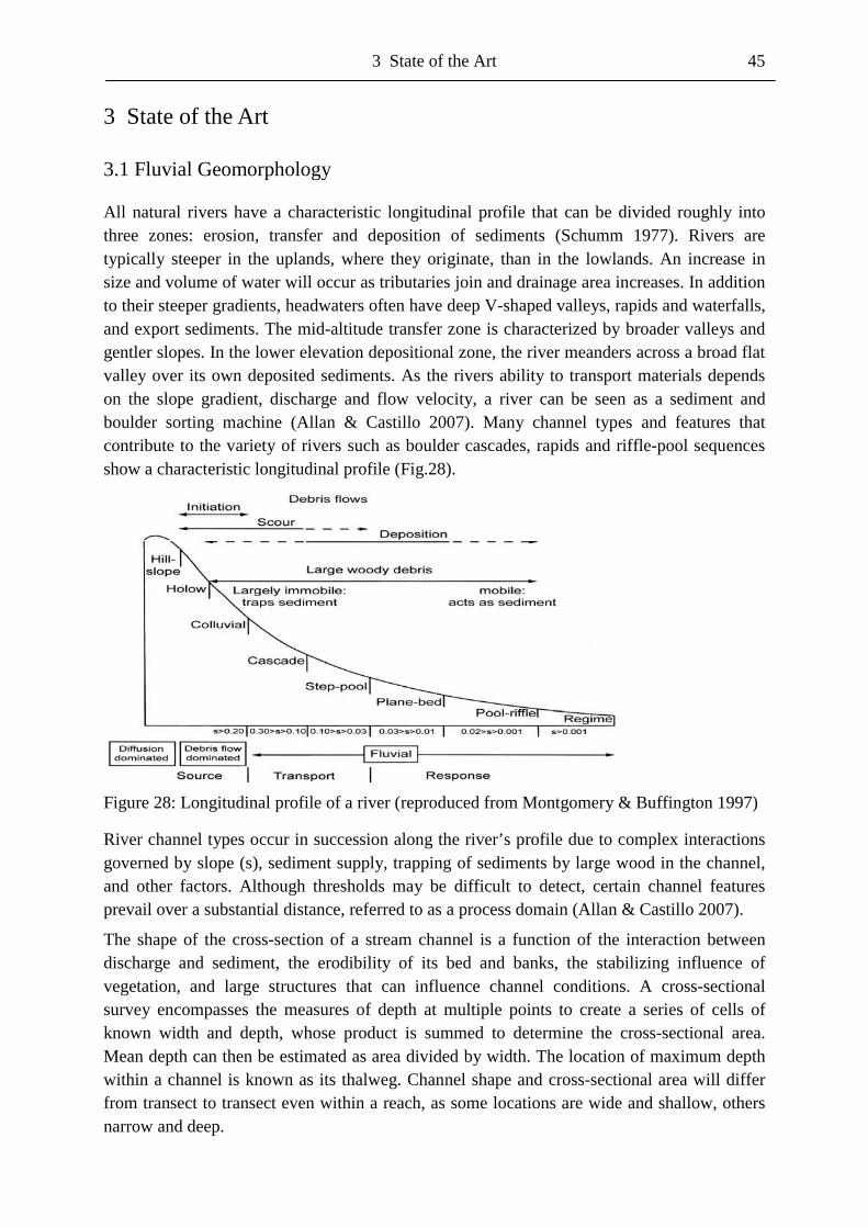
3 State of the Art 45

3 State of the Art 3.1 Fluvial Geomorphology

All natural rivers have a characteristic longitudinal profile that can be divided roughly into three zones: erosion, transfer and deposition of sediments (Schumm 1977). Rivers are typically steeper in the uplands, where they originate, than in the lowlands. An increase in size and volume of water will occur as tributaries join and drainage area increases. In addition to their steeper gradients, headwaters often have deep V-shaped valleys, rapids and waterfalls, and export sediments. The mid-altitude transfer zone is characterized by broader valleys and gentler slopes. In the lower elevation depositional zone, the river meanders across a broad flat valley over its own deposited sediments. As the rivers ability to transport materials depends on the slope gradient, discharge and flow velocity, a river can be seen as a sediment and boulder sorting machine (Allan & Castillo 2007). Many channel types and features that contribute to the variety of rivers such as boulder cascades, rapids and riffle-pool sequences show a characteristic longitudinal profile (Fig.28).

Figure 28: Longitudinal profile of a river (reproduced from Montgomery & Buffington 1997)

River channel types occur in succession along the river’s profile due to complex interactions governed by slope (s), sediment supply, trapping of sediments by large wood in the channel, and other factors. Although thresholds may be difficult to detect, certain channel features prevail over a substantial distance, referred to as a process domain (Allan & Castillo 2007).

The shape of the cross-section of a stream channel is a function of the interaction between discharge and sediment, the erodibility of its bed and banks, the stabilizing influence of vegetation, and large structures that can influence channel conditions. A cross-sectional survey encompasses the measures of depth at multiple points to create a series of cells of known width and depth, whose product is summed to determine the cross-sectional area. Mean depth can then be estimated as area divided by width. The location of maximum depth within a channel is known as its thalweg. Channel shape and cross-sectional area will differ from transect to transect even within a reach, as some locations are wide and shallow, others narrow and deep.

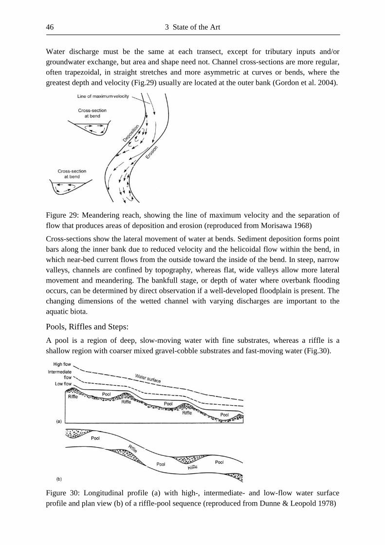
46 3 State of the Art

Water discharge must be the same at each transect, except for tributary inputs and/or groundwater exchange, but area and shape need not. Channel cross-sections are more regular, often trapezoidal, in straight stretches and more asymmetric at curves or bends, where the greatest depth and velocity (Fig.29) usually are located at the outer bank (Gordon et al. 2004).

Figure 29: Meandering reach, showing the line of maximum velocity and the separation of flow that produces areas of deposition and erosion (reproduced from Morisawa 1968)

Cross-sections show the lateral movement of water at bends. Sediment deposition forms point bars along the inner bank due to reduced velocity and the helicoidal flow within the bend, in which near-bed current flows from the outside toward the inside of the bend. In steep, narrow valleys, channels are confined by topography, whereas flat, wide valleys allow more lateral movement and meandering. The bankfull stage, or depth of water where overbank flooding occurs, can be determined by direct observation if a well-developed floodplain is present. The changing dimensions of the wetted channel with varying discharges are important to the aquatic biota.

Pools, Riffles and Steps:

A pool is a region of deep, slow-moving water with fine substrates, whereas a riffle is a shallow region with coarser mixed gravel-cobble substrates and fast-moving water (Fig.30).

Figure 30: Longitudinal profile (a) with high-, intermediate- and low-flow water surface profile and plan view (b) of a riffle-pool sequence (reproduced from Dunne & Leopold 1978)

3 State of the Art 47

The riffle is a topographical hillock and the pool a depression in a wavelike streambed. At riffles, the cross-sectional profiles tend to be rectangular, whereas pools show more asymmetric profiles. The term run is sometimes given to an intermediate category in which the flow is less turbulent than in riffles but moves faster than in pools. Pools and riffles alternate, whereas the depth of the pool is controlled by the elevation of the following riffle downstream, so that together they can be considered ‘vertical meanders’ (Knighton 1984). This pool-riffle periodicity may be important in the cycling of nutrients along a stream (Goldman & Horne 1983). Pool-riffle channels typically are found in moderate to low gradient, unconfined, meandering gravel-bed streams, with pools located at meander bends and riffles at crossover stretches. In self-formed pool-riffle channels, riffles are formed by the deposition of gravel bars in a characteristic alternation from one side of the channel to the other, at a typical distance of about 5 - 7 channel widths (Leopold et al. 1964). Irregular rhythmic patterns can result from local controls such as bedrock constrictions or tree roots, or an increased supply of coarse sediments. This semi-regular pattern is also found in straight channels, bedrock streams and the dried remains of semi-arid ephemeral streambeds. In steep, boulder-bed mountain streams the pool-riffle sequence is replaced by a pool-step sequence, where water tumbles over accumulations of boulders and short waterfalls plunge into small scour pools. ‘Organic’ steps can also be created by large fallen trees or debris dams. This debris-created steps also tend to be regularly spaced (Morisawa 1985).

Pool-riffle sequences are the result of particle sorting and require a range of sediment sizes to develop. Alternating pool-riffle sequences are most common in streams with mixed bed materials ranging from 2 - 256 mm (Knighton 1984). Steps, riffles and pools become more important at low flows when they become more dominant components of channel geometry. At low flow, riffles are shallower, have a higher slope and velocity compared to pools. At high flows the water surface slope, depth of flow and speed of the current between riffles and pools become more uniform, but pools remain deeper and velocity increases more in pools than in riffles. This results in changes in the distribution of forces on the streambed. As discharge increases, velocity and depth rise more rapidly in pools than in riffles, and energy loss becomes more uniform. The shear stress in pools can eventually exceed that in riffles, which may be part of a sorting mechanism for concentrating coarser materials in riffles (Knighton 1984). At flood stage, when flows are high enough to mobilize the bed, riffles are the locations of lowest transport capacity and thus the locations of gravel deposition, whereas coarse particles move from riffle to riffle, while very coarse fragments tend to deposit in the deepest part of pools (Gordon et al. 2004). Pool-riffle structures are usually formed by rare, large historic events, and pool-step systems may relate to even rarer, higher intensity discharges (Petts & Foster 1985). Thus, the flows which form these structures differ from those that maintain them, and they remain relatively stable under all but extreme flow conditions (Knighton 1984). Pools may deepen as a result of localized scour during low to moderate flows, especially at bends or the downstream side of logs, but they may also fill up with sediment if sediment supplies increase (Beschta & Platts 1986). Generally, pools form on the outside of bends and at locations where large woods or other obstructions force pool development (Leopold et al. 1964). In high gradient, gravel-bed streams of the Pacific Northwest U.S.A., the presence of pools is strongly dependent on large woods, and streams with a high loading of wood typically have closer pool spacing (Castillo & Allan 2007).

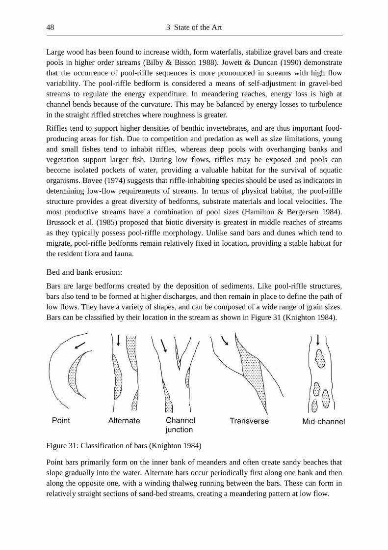
48 3 State of the Art

Large wood has been found to increase width, form waterfalls, stabilize gravel bars and create pools in higher order streams (Bilby & Bisson 1988). Jowett & Duncan (1990) demonstrate that the occurrence of pool-riffle sequences is more pronounced in streams with high flow variability. The pool-riffle bedform is considered a means of self-adjustment in gravel-bed streams to regulate the energy expenditure. In meandering reaches, energy loss is high at channel bends because of the curvature. This may be balanced by energy losses to turbulence in the straight riffled stretches where roughness is greater.

Riffles tend to support higher densities of benthic invertebrates, and are thus important food-producing areas for fish. Due to competition and predation as well as size limitations, young and small fishes tend to inhabit riffles, whereas deep pools with overhanging banks and vegetation support larger fish. During low flows, riffles may be exposed and pools can become isolated pockets of water, providing a valuable habitat for the survival of aquatic organisms. Bovee (1974) suggests that riffle-inhabiting species should be used as indicators in determining low-flow requirements of streams. In terms of physical habitat, the pool-riffle structure provides a great diversity of bedforms, substrate materials and local velocities. The most productive streams have a combination of pool sizes (Hamilton & Bergersen 1984). Brussock et al. (1985) proposed that biotic diversity is greatest in middle reaches of streams as they typically possess pool-riffle morphology. Unlike sand bars and dunes which tend to migrate, pool-riffle bedforms remain relatively fixed in location, providing a stable habitat for the resident flora and fauna. Bed and bank erosion:

Bars are large bedforms created by the deposition of sediments. Like pool-riffle structures, bars also tend to be formed at higher discharges, and then remain in place to define the path of low flows. They have a variety of shapes, and can be composed of a wide range of grain sizes. Bars can be classified by their location in the stream as shown in Figure 31 (Knighton 1984).

Figure 31: Classification of bars (Knighton 1984)

Point bars primarily form on the inner bank of meanders and often create sandy beaches that slope gradually into the water. Alternate bars occur periodically first along one bank and then along the opposite one, with a winding thalweg running between the bars. These can form in relatively straight sections of sand-bed streams, creating a meandering pattern at low flow.

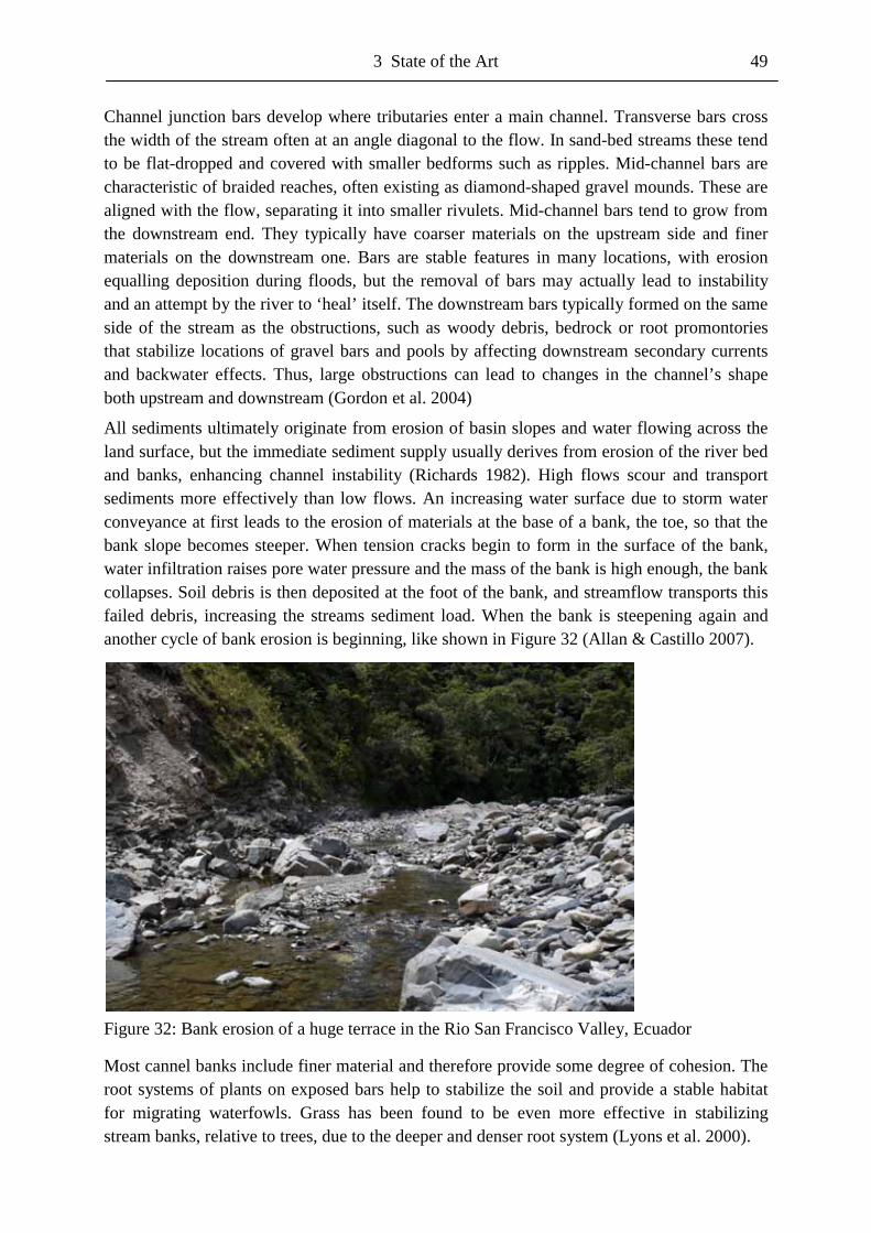
3 State of the Art 49

Channel junction bars develop where tributaries enter a main channel. Transverse bars cross the width of the stream often at an angle diagonal to the flow. In sand-bed streams these tend to be flat-dropped and covered with smaller bedforms such as ripples. Mid-channel bars are characteristic of braided reaches, often existing as diamond-shaped gravel mounds. These are aligned with the flow, separating it into smaller rivulets. Mid-channel bars tend to grow from the downstream end. They typically have coarser materials on the upstream side and finer materials on the downstream one. Bars are stable features in many locations, with erosion equalling deposition during floods, but the removal of bars may actually lead to instability and an attempt by the river to ‘heal’ itself. The downstream bars typically formed on the same side of the stream as the obstructions, such as woody debris, bedrock or root promontories that stabilize locations of gravel bars and pools by affecting downstream secondary currents and backwater effects. Thus, large obstructions can lead to changes in the channel’s shape both upstream and downstream (Gordon et al. 2004)

All sediments ultimately originate from erosion of basin slopes and water flowing across the land surface, but the immediate sediment supply usually derives from erosion of the river bed and banks, enhancing channel instability (Richards 1982). High flows scour and transport sediments more effectively than low flows. An increasing water surface due to storm water conveyance at first leads to the erosion of materials at the base of a bank, the toe, so that the bank slope becomes steeper. When tension cracks begin to form in the surface of the bank, water infiltration raises pore water pressure and the mass of the bank is high enough, the bank collapses. Soil debris is then deposited at the foot of the bank, and streamflow transports this failed debris, increasing the streams sediment load. When the bank is steepening again and another cycle of bank erosion is beginning, like shown in Figure 32 (Allan & Castillo 2007).

Figure 32: Bank erosion of a huge terrace in the Rio San Francisco Valley, Ecuador

Most cannel banks include finer material and therefore provide some degree of cohesion. The root systems of plants on exposed bars help to stabilize the soil and provide a stable habitat for migrating waterfowls. Grass has been found to be even more effective in stabilizing stream banks, relative to trees, due to the deeper and denser root system (Lyons et al. 2000).

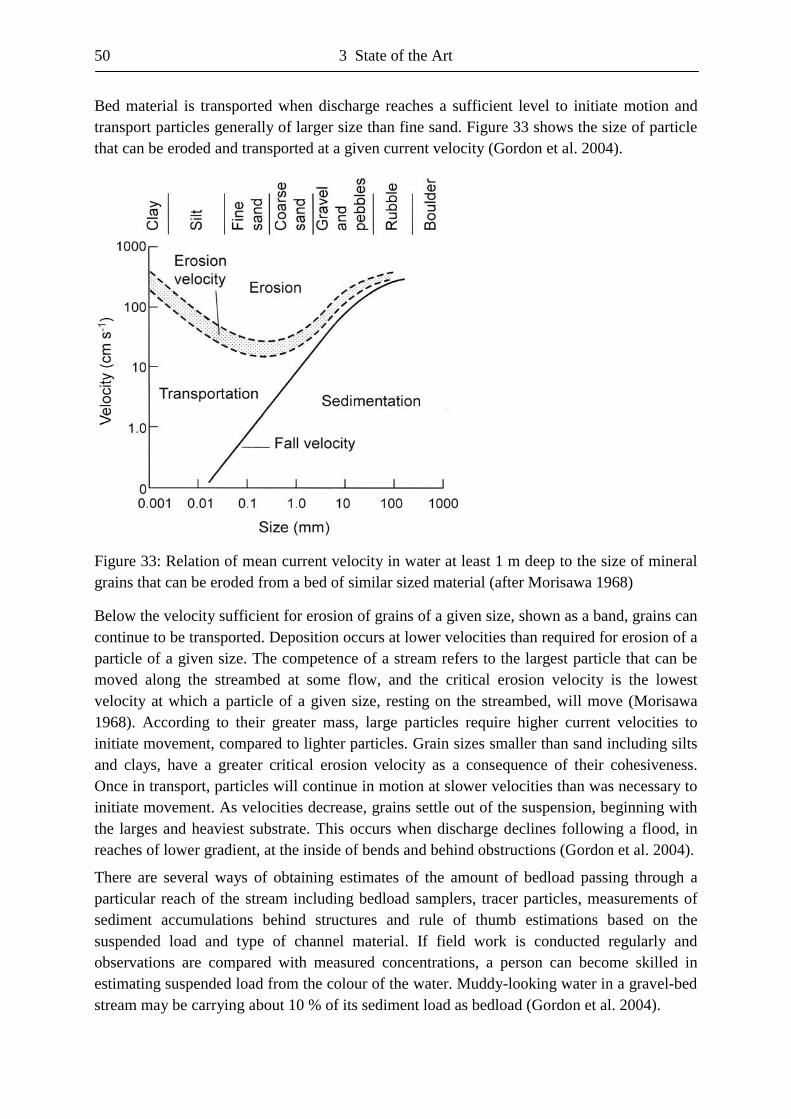
50 3 State of the Art

Bed material is transported when discharge reaches a sufficient level to initiate motion and transport particles generally of larger size than fine sand. Figure 33 shows the size of particle that can be eroded and transported at a given current velocity (Gordon et al. 2004).

Figure 33: Relation of mean current velocity in water at least 1 m deep to the size of mineral grains that can be eroded from a bed of similar sized material (after Morisawa 1968)

Below the velocity sufficient for erosion of grains of a given size, shown as a band, grains can continue to be transported. Deposition occurs at lower velocities than required for erosion of a particle of a given size. The competence of a stream refers to the largest particle that can be moved along the streambed at some flow, and the critical erosion velocity is the lowest velocity at which a particle of a given size, resting on the streambed, will move (Morisawa 1968). According to their greater mass, large particles require higher current velocities to initiate movement, compared to lighter particles. Grain sizes smaller than sand including silts and clays, have a greater critical erosion velocity as a consequence of their cohesiveness. Once in transport, particles will continue in motion at slower velocities than was necessary to initiate movement. As velocities decrease, grains settle out of the suspension, beginning with the larges and heaviest substrate. This occurs when discharge declines following a flood, in reaches of lower gradient, at the inside of bends and behind obstructions (Gordon et al. 2004).

There are several ways of obtaining estimates of the amount of bedload passing through a particular reach of the stream including bedload samplers, tracer particles, measurements of sediment accumulations behind structures and rule of thumb estimations based on the suspended load and type of channel material. If field work is conducted regularly and observations are compared with measured concentrations, a person can become skilled in estimating suspended load from the colour of the water. Muddy-looking water in a gravel-bed stream may be carrying about 10 % of its sediment load as bedload (Gordon et al. 2004).

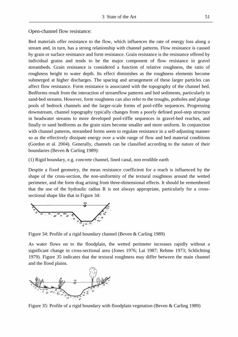
3 State of the Art 51

Open-channel flow resistance:

Bed materials offer resistance to the flow, which influences the rate of energy loss along a stream and, in turn, has a strong relationship with channel patterns. Flow resistance is caused by grain or surface resistance and form resistance. Grain resistance is the resistance offered by individual grains and tends to be the major component of flow resistance in gravel streambeds. Grain resistance is considered a function of relative roughness, the ratio of roughness height to water depth. Its effect diminishes as the roughness elements become submerged at higher discharges. The spacing and arrangement of these larger particles can affect flow resistance. Form resistance is associated with the topography of the channel bed. Bedforms result from the interaction of streamflow patterns and bed sediments, particularly in sand-bed streams. However, form roughness can also refer to the troughs, potholes and plunge pools of bedrock channels and the larger-scale forms of pool-riffle sequences. Progressing downstream, channel topography typically changes from a poorly defined pool-step structure in headwater streams to more developed pool-riffle sequences in gravel-bed reaches, and finally to sand bedforms as the grain sizes become smaller and more uniform. In conjunction with channel patterns, streambed forms seem to regulate resistance in a self-adjusting manner so as the effectively dissipate energy over a wide range of flow and bed material conditions (Gordon et al. 2004). Generally, channels can be classified according to the nature of their boundaries (Beven & Carling 1989): (1) Rigid boundary, e.g. concrete channel, lined canal, non erodible earth

Despite a fixed geometry, the mean resistance coefficient for a reach is influenced by the shape of the cross-section, the non-uniformity of the textural roughness around the wetted perimeter, and the form drag arising from three-dimensional effects. It should be remembered that the use of the hydraulic radius R is not always appropriate, particularly for a cross-sectional shape like that in Figure 34:

Figure 34: Profile of a rigid boundary channel (Beven & Carling 1989)

As water flows on to the floodplain, the wetted perimeter increases rapidly without a significant change in cross-sectional area (Jones 1976; Lai 1987; Rehme 1973; Schlichting 1979). Figure 35 indicates that the textural roughness may differ between the main channel and the flood plains.

Figure 35: Profile of a rigid boundary with floodplain vegetation (Beven & Carling 1989)

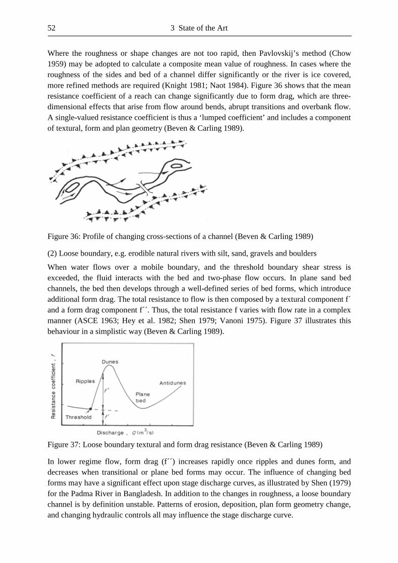
52 3 State of the Art

Where the roughness or shape changes are not too rapid, then Pavlovskij’s method (Chow 1959) may be adopted to calculate a composite mean value of roughness. In cases where the roughness of the sides and bed of a channel differ significantly or the river is ice covered, more refined methods are required (Knight 1981; Naot 1984). Figure 36 shows that the mean resistance coefficient of a reach can change significantly due to form drag, which are three-dimensional effects that arise from flow around bends, abrupt transitions and overbank flow. A single-valued resistance coefficient is thus a ‘lumped coefficient’ and includes a component of textural, form and plan geometry (Beven & Carling 1989).

Figure 36: Profile of changing cross-sections of a channel (Beven & Carling 1989)

(2) Loose boundary, e.g. erodible natural rivers with silt, sand, gravels and boulders

When water flows over a mobile boundary, and the threshold boundary shear stress is exceeded, the fluid interacts with the bed and two-phase flow occurs. In plane sand bed channels, the bed then develops through a well-defined series of bed forms, which introduce additional form drag. The total resistance to flow is then composed by a textural component f´ and a form drag component f´´. Thus, the total resistance f varies with flow rate in a complex manner (ASCE 1963; Hey et al. 1982; Shen 1979; Vanoni 1975). Figure 37 illustrates this behaviour in a simplistic way (Beven & Carling 1989).

Figure 37: Loose boundary textural and form drag resistance (Beven & Carling 1989)

In lower regime flow, form drag (f´´) increases rapidly once ripples and dunes form, and decreases when transitional or plane bed forms may occur. The influence of changing bed forms may have a significant effect upon stage discharge curves, as illustrated by Shen (1979) for the Padma River in Bangladesh. In addition to the changes in roughness, a loose boundary channel is by definition unstable. Patterns of erosion, deposition, plan form geometry change, and changing hydraulic controls all may influence the stage discharge curve.

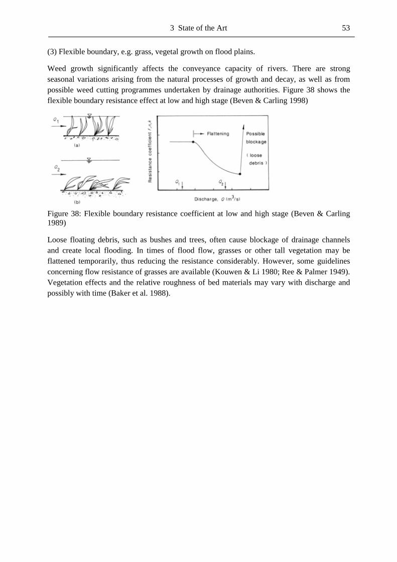
3 State of the Art 53

(3) Flexible boundary, e.g. grass, vegetal growth on flood plains.

Weed growth significantly affects the conveyance capacity of rivers. There are strong seasonal variations arising from the natural processes of growth and decay, as well as from possible weed cutting programmes undertaken by drainage authorities. Figure 38 shows the flexible boundary resistance effect at low and high stage (Beven & Carling 1998)

Figure 38: Flexible boundary resistance coefficient at low and high stage (Beven & Carling 1989)

Loose floating debris, such as bushes and trees, often cause blockage of drainage channels and create local flooding. In times of flood flow, grasses or other tall vegetation may be flattened temporarily, thus reducing the resistance considerably. However, some guidelines concerning flow resistance of grasses are available (Kouwen & Li 1980; Ree & Palmer 1949). Vegetation effects and the relative roughness of bed materials may vary with discharge and possibly with time (Baker et al. 1988).

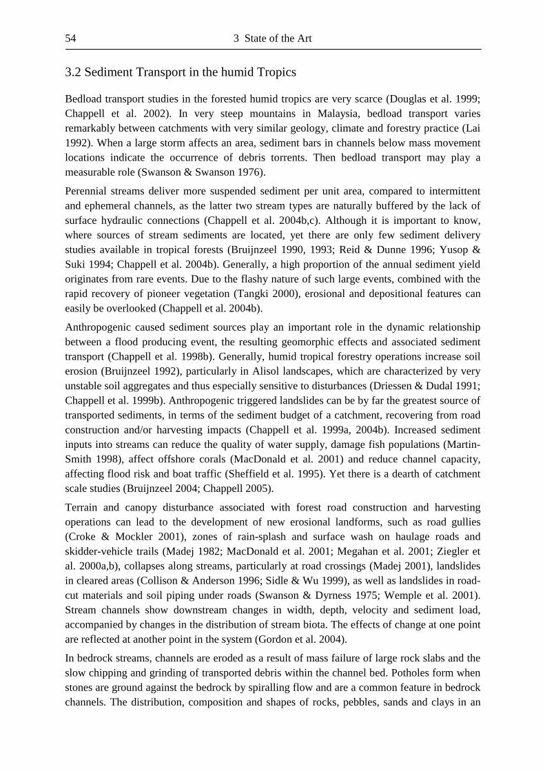
54 3 State of the Art

3.2 Sediment Transport in the humid Tropics

Bedload transport studies in the forested humid tropics are very scarce (Douglas et al. 1999; Chappell et al. 2002). In very steep mountains in Malaysia, bedload transport varies remarkably between catchments with very similar geology, climate and forestry practice (Lai 1992). When a large storm affects an area, sediment bars in channels below mass movement locations indicate the occurrence of debris torrents. Then bedload transport may play a measurable role (Swanson & Swanson 1976).

Perennial streams deliver more suspended sediment per unit area, compared to intermittent and ephemeral channels, as the latter two stream types are naturally buffered by the lack of surface hydraulic connections (Chappell et al. 2004b,c). Although it is important to know, where sources of stream sediments are located, yet there are only few sediment delivery studies available in tropical forests (Bruijnzeel 1990, 1993; Reid & Dunne 1996; Yusop & Suki 1994; Chappell et al. 2004b). Generally, a high proportion of the annual sediment yield originates from rare events. Due to the flashy nature of such large events, combined with the rapid recovery of pioneer vegetation (Tangki 2000), erosional and depositional features can easily be overlooked (Chappell et al. 2004b).

Anthropogenic caused sediment sources play an important role in the dynamic relationship between a flood producing event, the resulting geomorphic effects and associated sediment transport (Chappell et al. 1998b). Generally, humid tropical forestry operations increase soil erosion (Bruijnzeel 1992), particularly in Alisol landscapes, which are characterized by very unstable soil aggregates and thus especially sensitive to disturbances (Driessen & Dudal 1991; Chappell et al. 1999b). Anthropogenic triggered landslides can be by far the greatest source of transported sediments, in terms of the sediment budget of a catchment, recovering from road construction and/or harvesting impacts (Chappell et al. 1999a, 2004b). Increased sediment inputs into streams can reduce the quality of water supply, damage fish populations (Martin-Smith 1998), affect offshore corals (MacDonald et al. 2001) and reduce channel capacity, affecting flood risk and boat traffic (Sheffield et al. 1995). Yet there is a dearth of catchment scale studies (Bruijnzeel 2004; Chappell 2005).

Terrain and canopy disturbance associated with forest road construction and harvesting operations can lead to the development of new erosional landforms, such as road gullies (Croke & Mockler 2001), zones of rain-splash and surface wash on haulage roads and skidder-vehicle trails (Madej 1982; MacDonald et al. 2001; Megahan et al. 2001; Ziegler et al. 2000a,b), collapses along streams, particularly at road crossings (Madej 2001), landslides in cleared areas (Collison & Anderson 1996; Sidle & Wu 1999), as well as landslides in road-cut materials and soil piping under roads (Swanson & Dyrness 1975; Wemple et al. 2001). Stream channels show downstream changes in width, depth, velocity and sediment load, accompanied by changes in the distribution of stream biota. The effects of change at one point are reflected at another point in the system (Gordon et al. 2004).

In bedrock streams, channels are eroded as a result of mass failure of large rock slabs and the slow chipping and grinding of transported debris within the channel bed. Potholes form when stones are ground against the bedrock by spiralling flow and are a common feature in bedrock channels. The distribution, composition and shapes of rocks, pebbles, sands and clays in an

3 State of the Art 55

alluvial channel bed reflect the hydraulics of high and low flows. Due to the fact that weak rocks, such as mudstone, shale or sandstone are and more easily broken up and rounded than the less erosive quartzite, the size of sediments and the distance they have travelled reveal the hydrological stream evolution. In headwater regions, large angular bed materials that exceed the competence of a stream often decay near their origin. In a downstream direction, the mean grain size of substrate materials generally decreases as sediments are fragmented and abraded. The spatial distribution of bed materials is closely related to previous flood events.

Total load or debris load refers to the amount of dissolved and particulate organic and inorganic material carried by the stream. The total load can be divided into flotation load, dissolved load and sediment load. Commonly, sediment load is separated into suspended washload and bed load. Sediment is usually considered to be the solid inorganic material (Gordon et al 2004).

Flotation load consists of logs, leaves, branches and other organic debris, generally being lighter than water. The amount of organic debris supplied to a stream depends on the density and type of vegetation along the banks, the amount of bank failure and tree fall, and the amount of floating debris picked up from the floodplain by flood waters. Organic debris is the basic foodstuff of decomposers and some aquatic invertebrates. Large trees, roots and saplings provide shelter for fish, and form debris dams which trap sediments and modify the channel shape. Large woody debris can play an important role in channel stabilization. Removal of riparian vegetation reduces the supply of organic material to the stream, which may have long-term effects on its ecology and morphology. Flotation load can damage bridges and other man-made structures (Allan & Castillo 2007)

Dissolved load is the material transported by the stream in solution. Natural origins of dissolved loads include the chemical weathering of rocks and for example sea salts contained in rainwater in coastal regions. Generally, water originating as groundwater tends to have a higher soluble load than surface-derived runoff. On average, 38 % of the total load of the world’s rivers is dissolved material (Knighton 1984). As a consequence of turbulence, dissolved loads generally are uniformly distributed over a cross-sectional profile. Dissolved loads change with alternating discharge. During a runoff event, concentrations generally decrease at first as rainwater dilutes the stream water, but later increase as groundwater reaches the stream, delivering dissolved materials (Hjulstrom 1939).

Washload refers to the smaller sediments, primarily clays, silts and fine sands, which are readily carried in suspension by the stream. This load is ‘washed’ into the stream from the banks and upland areas and carried at essentially the same speed as the water. Only low velocities and minor turbulence are required to keep it in suspension, and it may never settle out. Its concentration is considered constant over the depth of a stream. The supply of washload from upstream sources determines the amount of transported washload and there is no limiting transport capacity for washload, because streams cannot become ‘saturated’ with sediment (Hjulstrom 1939). The washload can constitute a large percentage of the total volume and mass carried by a river. High washload is typical for streams with banks of high silt-clay content and for fired-denuded slopes. Furthermore, ashes from volcanic eruptions, road construction and agricultural use can provide significant amounts of washload.

56 3 State of the Art

Bedload is the material which generally remains in contact with the streambed, moves by rolling, sliding or hopping, also called saltation, and has about the same size range as streambed particles. Bedload movement is important because of its relationship to changes in the bars and bends of a stream’s morphology. It is also important to benthic stream biota which can be crushed or distributed by the moving material. Suspended bed-material load is the portion that is carried with the washload, remaining in suspension for an appreciable length of time. It is supported by the fluid and kept aloft by turbulent eddies, but will settle out quickly when velocities drop (Gordon et al. 2004). Finer materials than sand, such as silts and clays tend to be uniformly distributed in a cross-section, while coarser bedload material is concentrated near the streambed (Richards 1982). The actual distribution over a particular vertical in a stream is dependent on the particles sizes, particle concentration, as well as the velocity and turbulence intensity of the water flow. The largest quantities of sediment and the coarsest fractions tend to be transported in the path of maximum velocity. If velocity and turbulence increase, the larger particles will be distributed more evenly. On average, less bedload than suspended load is transported over a year (Gordon et al. 2004).

In sediment source areas, surface erosion is usually highest in the beginning of a rainstorm, as available sediments are washed quickly into the stream via overland flow. Washload fines typically occur in higher concentration at the beginning of an event. When the sediment supply becomes exhausted, the concentration drops quickly so that the sediment concentration in the rising limb of a hydrograph is generally higher, compared to the falling limb. This effect is called hysteresis. In headwater areas the sediment concentration will typically peak before discharge does. Bedload movement and entrainment of bed materials increases as the discharge reaches its peak, and then a reduction in particle size occurs as the hydrograph declines. The amount of sediment carried through the outlet of a catchment depends on the available amount and type of sediment eroded and transported to the stream from upland sources and the ability of a stream to carry the washed-in sediments and to re-work and transport bed and bank materials. Therefore, streams can be considered either supply-limited or capacity-limited, depending on whether their ability to carry sediment exceeds the amount available or vice versa. In regard to the type of sediment carried, washload is considered supply-limited and bed-material load capacity-limited. Mountain channels with large streambed materials and pool-step structures are typically supply-limited (Gordon et al. 2004). The relationship between runoff processes and the initiation of natural drainage networks, and the implications on sediment delivery have been reviewed by Dunne (1980) and Jones (1987). Soil moisture levels are closely linked with the occurrence of mass movements, especially on convergent hillslope hollows (Freeze 1986). In Japanese mountains more than 80 % of debris slides occurred on convergent slopes (Tsukamoto et al. 1982). The delivery of sediment to the stream channel by mass movement can significantly affect the geomorphological effectiveness of both present and future floods (Newson 1980). At the basin scale, the spatial pattern of stream solutes depends, on climate, lithology, soil and land use (Walling & Webb 1975), whereas at the sub-catchment scale, topography and land use are important controls (Burt & Arkell 1986, 1987).

3 State of the Art 57

Ecology:

For many aquatic organisms the channel bed is a substrate to be used as a foothold, as a sit to deposit or incubate eggs, as grit for grinding food or as a refuge from floods (Minshall 1984; Statzner et al. 1988). The surface of the streambed is rich in organic matter, providing nutrients for organisms at the base of the food chain. Below the surface, the normally biological active hyporheic zone forms an interface between stream and groundwater systems, where organisms temporarily reside or spend their whole life cycle deep within stony streambeds (Hynes 1970). The streambed acts as a refuge for benthic organisms, providing shelter from floods, drought, fluctuating temperatures and is capable to recolonize the stream if stream populations are depleted by adverse conditions (Ward & Stanford 1983a). The suitability of a substrate for colonization by aquatic flora and fauna depends on its average particle size, its mix of sizes, size of pore spaces, degree of packing and imbeddedness, and its surface topography. Freshwater crayfish and some aquatic insect species such as dragonfly and stonefly larvae live in the crevices between and beneath rocks. Caddisflies require unstable fine-grained sand, midge larvae require mud and salmons require a mix of gravels with small amounts of fine sediments and rubble (Beschta & Platts 1986). Algae, mosses and other aquatic plants also have specific substrate requirements and provide sheltering and supporting substrate for other organisms. Thus, the distribution of sediment sizes has an important influence on physical habitat conditions. In general, the highest productivity and diversity of aquatic invertebrates seems to occur in riffle habitats with medium cobble and gravel substrate (Gore 1985a). Areas of shifting sands commonly have reduced species abundance and richness (Minshall 1984). If large amounts of fine substrate are washed into a stream, they can form a ‘mat’ or ‘hardpan’ layer on top of the coarser bed materials, reducing inter-gravel flow velocity and thus affect biological activity, nutrient and oxygen supply, removal of metabolic waste, suffocate eggs, limit burrowing activity and trap emerging young. Gravel-bed streams that become filled with silt may experience a shift in the insect species compositions from mayflies and caddisflies to midgefly larvae, which may affect fish species composition (Milhous 1982). Thus, the transport of particulate matter is both bane and benefit to aquatic organisms. Organic particulate matter is a important food source for downstream organisms, but during flood stages, larger grains can become deadly projectiles. Fine silts and clays clog gills, reduce light needed for photosynthesis and periphyton production, and interfere with the foraging success of sight feeders and filterers. The shifting of whole segments of the streambed uproots and scours away benthic organisms. Heavy metals and other toxic substances can also be absorbed onto sediment and are thus transported and deposited along with it (Gordon et al. 2004). Vogel (1981) implies that abrasion and alterations of form of the stream bottom during floods have more critical impacts on biota than velocity. Jowett & Richardson (1989) cited a study on rivers in New Zealand where the abundance of trout decreased significantly after a major flood, although the coarsening of substrate, removal of excessive algae growth and deepening of pools improved habitat for future use. After floods, recolonization by bacteria, fungi and algae binds and stabilizes the substrate, improving conditions so that other organisms can come back more quickly. Variations of velocity with time may be critical to the aquatic insects (Gordon et al. 2004).

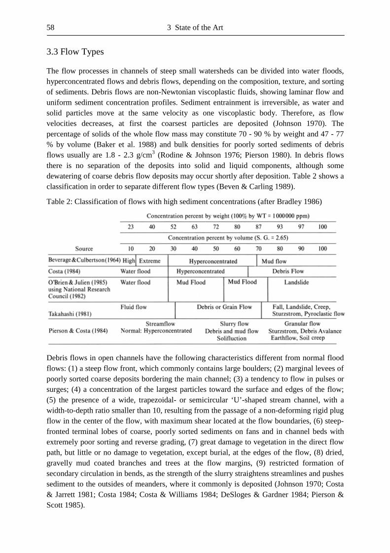
58 3 State of the Art

3.3 Flow Types

The flow processes in channels of steep small watersheds can be divided into water floods, hyperconcentrated flows and debris flows, depending on the composition, texture, and sorting of sediments. Debris flows are non-Newtonian viscoplastic fluids, showing laminar flow and uniform sediment concentration profiles. Sediment entrainment is irreversible, as water and solid particles move at the same velocity as one viscoplastic body. Therefore, as flow velocities decreases, at first the coarsest particles are deposited (Johnson 1970). The percentage of solids of the whole flow mass may constitute 70 - 90 % by weight and 47 - 77 % by volume (Baker et al. 1988) and bulk densities for poorly sorted sediments of debris flows usually are 1.8 - 2.3 g/cm3 (Rodine & Johnson 1976; Pierson 1980). In debris flows there is no separation of the deposits into solid and liquid components, although some dewatering of coarse debris flow deposits may occur shortly after deposition. Table 2 shows a classification in order to separate different flow types (Beven & Carling 1989). Table 2: Classification of flows with high sediment concentrations (after Bradley 1986)

Debris flows in open channels have the following characteristics different from normal flood flows: (1) a steep flow front, which commonly contains large boulders; (2) marginal levees of poorly sorted coarse deposits bordering the main channel; (3) a tendency to flow in pulses or surges; (4) a concentration of the largest particles toward the surface and edges of the flow; (5) the presence of a wide, trapezoidal- or semicircular ‘U’-shaped stream channel, with a width-to-depth ratio smaller than 10, resulting from the passage of a non-deforming rigid plug flow in the center of the flow, with maximum shear located at the flow boundaries, (6) steep-fronted terminal lobes of coarse, poorly sorted sediments on fans and in channel beds with extremely poor sorting and reverse grading, (7) great damage to vegetation in the direct flow path, but little or no damage to vegetation, except burial, at the edges of the flow, (8) dried, gravelly mud coated branches and trees at the flow margins, (9) restricted formation of secondary circulation in bends, as the strength of the slurry straightens streamlines and pushes sediment to the outsides of meanders, where it commonly is deposited (Johnson 1970; Costa & Jarrett 1981; Costa 1984; Costa & Williams 1984; DeSloges & Gardner 1984; Pierson & Scott 1985).

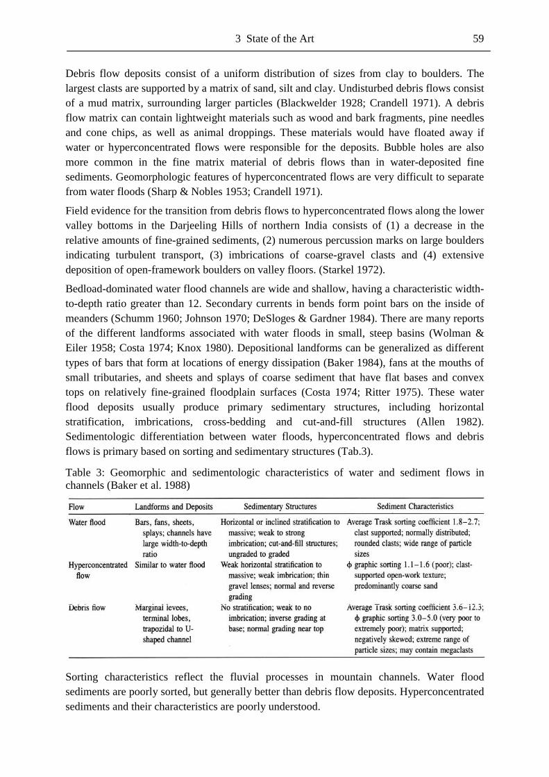
3 State of the Art 59

Debris flow deposits consist of a uniform distribution of sizes from clay to boulders. The largest clasts are supported by a matrix of sand, silt and clay. Undisturbed debris flows consist of a mud matrix, surrounding larger particles (Blackwelder 1928; Crandell 1971). A debris flow matrix can contain lightweight materials such as wood and bark fragments, pine needles and cone chips, as well as animal droppings. These materials would have floated away if water or hyperconcentrated flows were responsible for the deposits. Bubble holes are also more common in the fine matrix material of debris flows than in water-deposited fine sediments. Geomorphologic features of hyperconcentrated flows are very difficult to separate from water floods (Sharp & Nobles 1953; Crandell 1971).

Field evidence for the transition from debris flows to hyperconcentrated flows along the lower valley bottoms in the Darjeeling Hills of northern India consists of (1) a decrease in the relative amounts of fine-grained sediments, (2) numerous percussion marks on large boulders indicating turbulent transport, (3) imbrications of coarse-gravel clasts and (4) extensive deposition of open-framework boulders on valley floors. (Starkel 1972).

Bedload-dominated water flood channels are wide and shallow, having a characteristic width-to-depth ratio greater than 12. Secondary currents in bends form point bars on the inside of meanders (Schumm 1960; Johnson 1970; DeSloges & Gardner 1984). There are many reports of the different landforms associated with water floods in small, steep basins (Wolman & Eiler 1958; Costa 1974; Knox 1980). Depositional landforms can be generalized as different types of bars that form at locations of energy dissipation (Baker 1984), fans at the mouths of small tributaries, and sheets and splays of coarse sediment that have flat bases and convex tops on relatively fine-grained floodplain surfaces (Costa 1974; Ritter 1975). These water flood deposits usually produce primary sedimentary structures, including horizontal stratification, imbrications, cross-bedding and cut-and-fill structures (Allen 1982). Sedimentologic differentiation between water floods, hyperconcentrated flows and debris flows is primary based on sorting and sedimentary structures (Tab.3). Table 3: Geomorphic and sedimentologic characteristics of water and sediment flows in channels (Baker et al. 1988)

Sorting characteristics reflect the fluvial processes in mountain channels. Water flood sediments are poorly sorted, but generally better than debris flow deposits. Hyperconcentrated sediments and their characteristics are poorly understood.

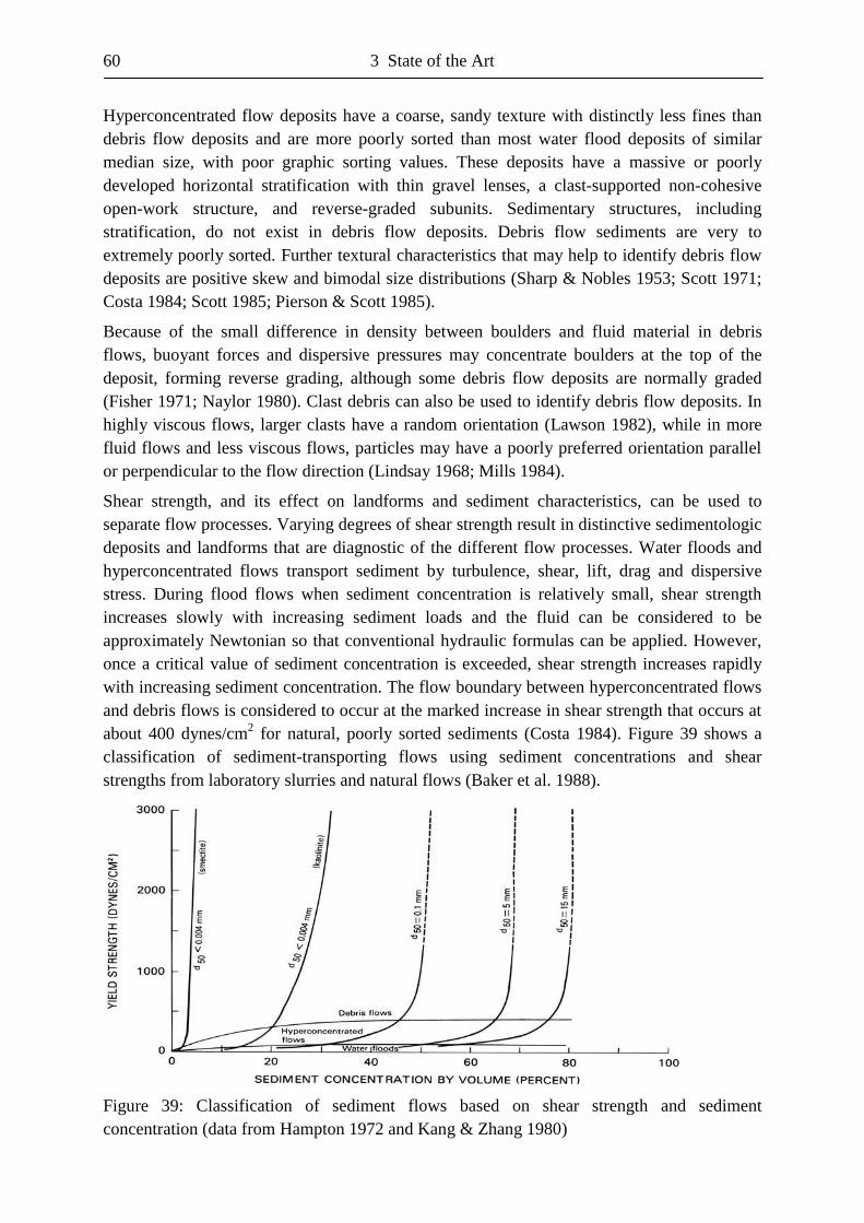
60 3 State of the Art

Hyperconcentrated flow deposits have a coarse, sandy texture with distinctly less fines than debris flow deposits and are more poorly sorted than most water flood deposits of similar median size, with poor graphic sorting values. These deposits have a massive or poorly developed horizontal stratification with thin gravel lenses, a clast-supported non-cohesive open-work structure, and reverse-graded subunits. Sedimentary structures, including stratification, do not exist in debris flow deposits. Debris flow sediments are very to extremely poorly sorted. Further textural characteristics that may help to identify debris flow deposits are positive skew and bimodal size distributions (Sharp & Nobles 1953; Scott 1971; Costa 1984; Scott 1985; Pierson & Scott 1985).

Because of the small difference in density between boulders and fluid material in debris flows, buoyant forces and dispersive pressures may concentrate boulders at the top of the deposit, forming reverse grading, although some debris flow deposits are normally graded (Fisher 1971; Naylor 1980). Clast debris can also be used to identify debris flow deposits. In highly viscous flows, larger clasts have a random orientation (Lawson 1982), while in more fluid flows and less viscous flows, particles may have a poorly preferred orientation parallel or perpendicular to the flow direction (Lindsay 1968; Mills 1984).

Shear strength, and its effect on landforms and sediment characteristics, can be used to separate flow processes. Varying degrees of shear strength result in distinctive sedimentologic deposits and landforms that are diagnostic of the different flow processes. Water floods and hyperconcentrated flows transport sediment by turbulence, shear, lift, drag and dispersive stress. During flood flows when sediment concentration is relatively small, shear strength increases slowly with increasing sediment loads and the fluid can be considered to be approximately Newtonian so that conventional hydraulic formulas can be applied. However, once a critical value of sediment concentration is exceeded, shear strength increases rapidly with increasing sediment concentration. The flow boundary between hyperconcentrated flows and debris flows is considered to occur at the marked increase in shear strength that occurs at about 400 dynes/cm2 for natural, poorly sorted sediments (Costa 1984). Figure 39 shows a classification of sediment-transporting flows using sediment concentrations and shear strengths from laboratory slurries and natural flows (Baker et al. 1988).

Figure 39: Classification of sediment flows based on shear strength and sediment concentration (data from Hampton 1972 and Kang & Zhang 1980)

3 State of the Art 61

The fundamental differences in rheology among the different flow processes, allows the reconstruction of the correct flow process from geomorphic and sedimentologic evidence. Hyperconcentrated flow landforms and deposits are transitional between more normal water floods and debris flows. They have been difficult to identify as causing unique landforms and deposits because such flows are relatively rare and transitional (Baker et al. 1988). The critical values of shear strength and sediment concentration between hyperconcentrated flows and debris flows vary with composition, texture, and sorting of sediments, and no single value can differentiate all situations. In debris flows, shear stress is concentrated in a thin zone at flow boundaries and sediment is transported by cohesive strength, buoyant forces, grain interactions, structural support and perhaps turbulence. Cohesion is controlled by the amount of clay in the debris. Buoyancy, controlled by the density difference of submerged solids and transporting fluid, is a major particle support mechanism in debris flows and could support 75 - 90 % of the particle weight in debris flows (Costa 1984). Dispersive stress (Bagnold 1954) results from lift produced when forces are transmitted between particles in collision or near collision as one is sheared over another. Where sediment concentrations are large, dispersive stress is a dominant process in dynamic sediment flows. Structural support, or grain-to-grain contacts providing a framework of particles in contact with the bed and each other, occurs at sediment volume concentrations greater than 35 % and supports about one-third of the weight of coarse particles (Pierson 1981). The efficiency of turbulence in debris flows is questionable because of the substantial viscosity and cohesion, as well as the laminar appearance of most debris flows (Enos 1977).

Mixtures of water, clay, silt, sand and rock particles can be considered as suspensions. The Coulomb-viscous and Bingham-plastic models that describe debris flows generally are known as viscoplastic rheology models. They originated from rheology investigations by Bingham & Green (1919) on oil paints and characterize features of debris flows and their deposits better than Newtonian models (Johnson 1970). In debris flows, resistance to flow or deformation results from shear strength originating from cohesion, internal friction and viscosity. Cohesion and internal friction constitute the yield strength of the debris that must be exceeded before any flow occurs. Viscosity only affects flow resistance in moving debris flows.

Debris flow rheology model approaches can be distinguishing into phenomenological and physical approaches. Phenomenological approaches have been developed by Johnson (1970), Fei (1982), Naik (1983), O’Brien & Julien (1988) and Wang Z. et al. (1992) in several rheometric experiments with mixtures of water and fine fraction debris flows. They concluded that a Bingham model or Coulomb-viscous model, in which debris flow is considered as a mixture of soil, following the Coulomb equation, and a Newtonian fluid, following the Newtonian viscous-flow equation, was best for describing the main characteristics of mud-mixture flow behaviour:

γηττ �*+= c (2)

where � = shear stress, �c = yield stress, � = viscosity and �� = shear rate.

62 3 State of the Art

Wang Y. (1989) and Major & Pierson (1992) in a similar approach used a Herschel-Bulkley model to describe the behaviour of mixtures of water and fine fraction debris flows:

nc K γττ �*+= (3)

where K, n = parameters of the fluid. Wang Y. (1989) suggested that the yield stress should be regarded as the sum of a term originating in matrix cohesion in a very fine sediment-water mixture and a term originating in friction between coarser particles. Major & Pierson (1992) tested mud-mixtures, fitted a Herschel-Bulkley model to their results and obtained a wide range of variation for the parameter n depending on material and solid concentration. Similarly, Phillips & Davies (1989, 1991) reported considerable fluctuations for very coarse suspensions. According to the authors, this phenomenon is caused by grain collisions and structural packing changes within the fluid.

A physical approach has been developed by Takahashi (1978, 1980, 1981), who applied the model that Bagnold (1954) developed for suspensions of particles in a Newtonian fluid to debris flows. The model distinguishes two regimes, whereas in the ‘Macro-viscous regime’ the viscous dissipation in the interstitial fluid prevails:

γηλτ �***25,2 5.1= for N < 40 (4) In the ‘Inertial regime’ the transfer momentum through inter-particle collision prevails:

22 **)*(* γησλρτ �Sa= for N > 450 (5)

where γρηλ

�*** 2DN S= , � = shear stress, 3 1)/(

1−

=vm CC

λ , � = viscosity, �� = shear rate

of the interstitial fluid, a = empirical coefficient, � = surface tension, �S = particle density, D = particle diameter, Cm = max. solid packing concentration, Cv = solid volumic concentration.

Takahashi (1991) proposed a yield criterion on the subject of debris flow motion initiation. Although all underlying ideas in the model are justified, it does not include both fluid yield stress and additional energy dissipation caused by motion. Additionally, the inertial regime does not consider turbulences within the interstitial fluid and momentum transfer. It is doubtful if natural debris flows can flow in an inertial regime, because the solid concentration is so high that the mean free path of particles is not large enough for collisions to prevail. Under these conditions, according to Bagnold’s theory, debris flow behaviour is in the Macro-viscous regime (Davies 1986). However, a viscous model only considering interstitial fluid energy dissipation is too simple, especially when particle friction or flocculent water-clay structure can exist. Similar problems occur in Chen’s (1988a, 1988b, 1991) generalized viscoplastic model for natural flow prediction. It is doubtful, if a single rheological model can be used to describe debris flow behaviour, because of the various complex components of debris flows suspensions (Phillips & Davies 1991; Coussot & Piau 1994).

3 State of the Art 63

Classification of natural debris flow suspension behaviour:

Coussot & Piau (1994) developed a classification based on well-known rheological results to characterize the qualitative behaviour of different natural mixtures. They defined physical boundary conditions and fundamental rheological characteristics of various natural suspensions to divide them in terms of their different qualitative behaviour. The classification assumes that it is possible to distinguish debris flow particles into two groups and that solid particle density is equal to water density. The first group includes particles for which the clay type interaction prevails, and the second group includes particles for which the coarse particle type interaction prevails. The coarsest particles, which interact either hydro-dynamically or directly through friction and/or collision when they are in close contact, are called force-free particles. Clay particles may interact through bounded water in ionized double-layers. A description of the nature of these interactions, which depends very much on pH, electrolyte concentration and clay type, is given by Wang et al. (1992). The classification distinguishes eight types of flows (Coussot & Piau 1994). (1) Pure water, few and more force-free particles in water

Pure water behaviour is Newtonian, but at high shear rates, fluctuating motions of particles around their mean motion appear. When the solid concentration is low enough, shearing motion of the interstitial fluid is slightly disturbed. Then theoretical calculations of total energy dissipation may be carried out for simple cases such as spheres or ellipsoids (Einstein 1956; Batchelor 1970). The resulting behaviour is Newtonian with a viscosity slightly higher than the interstitial fluid viscosity. As the concentration of force-free particles increases, hydrodynamic interaction between particles, friction and collisions have a greater influence on behaviour, but the behaviour will be still Newtonian (Kamal & Mutel 1985; Utracki 1988). (2) Percolating concentration of force-free particles

When the solid concentration is high enough, direct interaction and collision is very likely to prevail at high shear rates. Beyond a critical concentration, a continuous network of frictional particle contacts takes place throughout the sample. In order to break this network and initiate flow, it is necessary to impose a certain yield stress (Barnes et al. 1991, Kytomaa & Prasad 1993, Coussot 1992a). The solid concentration must not be too close to a maximum packing concentration or shear will be accompanied by shear thickening or dilatancy. (3) Few clay particles in water

The behaviour of double-layers is not well known, but at low clay concentrations and shear rates, the behaviour of the suspension is likely to be Newtonian. Viscosity is given by formulas formally identical to those obtained with force-free particle suspensions.

64 3 State of the Art

(4) More clay particles in water

Above a certain double-layer concentration, a continuous network of links due to repulsion and attraction between particles exists throughout the sample so that it is necessary to impose yield stress to initiate flow (M’Ewen & Mould 1957, Melton & Rand 1977). A Herschel-Bulkley model can be used, when interactions between particles are weak. For strong interactions, a micro-structural model, which describes the thixo-tropic behaviour of the rheology of concentrated dispersed systems in low weight matrix, and considers the evolution of broken bonds within the matrix, has been proposed by Coussot et al. (1992b, 1992c). (5) Clay-water mixtures with few force-free solid particles

There is no physical theory for predicting the behaviour of suspensions of force-free particles in yield stress fluids. However, assuming that the interstitial fluid follows a Bingham model and the force-free particle suspension follows the considerations of Newtonian fluid, an increase of the Bingham viscosity should result. Generally, when a simple Bingham model is used to describe the rheology of a suspension, the yield stress parameter corresponds to the minimum stress necessary to break the structure, which then results in a complex process of clay particle aggregate reformation and rupture. As a result, viscous dissipations originate in both phenomena and not only in classical hydrodynamic interactions. Migniot (1989), Major & Pierson (1992) and Coussot (1992a) observed that, the difference between the behaviour of the suspension and the behaviour of the interstitial fluid is negligible, when the concentration of force-free particles added to a clay-water mixture is not too high. (6) Clay-water mixtures with many force-free solid particles

Beyond a certain force-free particle concentration limit, effects of direct interaction prevail. In case of a Newtonian interstitial fluid, interaction was referred to as friction. Experiments of Coussot (1992a) proved that above a certain concentration of solid particles in a suspension there is a sudden increase of yield stress. As this percolation broadly corresponds to solid particle crowding, this rapid increase of yield stress is due to a sudden increase of the volume of frictional interactions between force-free particles (Coussot 1992a; Wang Y. 1989). (7) High force-free particle concentration in a clay water-mixture

When force-free particle concentration is too high the suspension can no longer stand large, continuous, incompressible deformation without a failure occurring through the sample. This phenomenon is clearly explained by the inability of a crowded, solid packing to change its configuration via an incompressible shear. The critical force-free particle concentration, beyond which this phenomenon appears, is lower than within an interstitial fluid such as water (Coussot & Piau 1994). (8) High force-free particle concentration in low clay water mixtures

If clay concentration in mixture (7) is decreased, a non-fracturing yield stress fluid results due to the lower viscosity of the interstitial fluid. When direct interactions between force-free particles are large, the suspension behaviour may be unstable (Coussot 1992a).

3 State of the Art 65

3.4 Geomorphic Impacts of Floods

Geomorphic response to large floods is controlled by numerous factors. In addition to basin and river channel factors, the recovery time between events is an important controlling factor of the response to large floods. The lasting impact of erosion by large floods on the extension and increased hydrologic efficiency of the drainage net is controlled by the recovery time of the basin (Wolman & Gerson 1978). If basin network extension, through the creation of new first-order channels, occurs at a greater rate than colluvial processes of channel abstraction, then the lag time of the basin should decrease, producing enhanced flood discharges that persist from one major storm to the next (Patton & Baker 1976; Baker 1977). Unlike the rapid and episodic network geometry changes in high relief basins, drainage basin evolution in low-relief regions is progressive. Over long time periods this may lead to a steady-state system with only slight variations in stream numbers, but varying network topology (Schumm 1956).

Drainage basin factors are external controls on the river channel and its floodplains, including: climate, hydrology, mainly peak discharge, contributing drainage area and hydrograph response, basin morphometry, sediment load, vegetation and soils. River channel factors are internal controls on the river, resulting from physical characteristics of the channel and flow, including: channel gradient, channel and floodplain geometry, channel morphology and bank cohesion (Baker et al. 1988).

Drainage Basin Factors:

Major floods usually result from one of four kinds of storms, which are tropical storms, convective storms associated with cold fronts, easterly waves and rainstorms due to orographic effects. Many areas of the world with arid or semi-arid climate, as well as humid regions that are not dominated by tropical influences are favoured to experience inland moving tropical storms that cause catastrophic floods. Major floods can also result from the passage of extra-tropical cyclones associated with cold fronts. These floods are most common in mid-latitude regions, where the interaction between cold polar air and warm tropical air masses is a common phenomenon. Major convective storms often develop along these cold fronts, which can result in significant rainfall amounts and severe flooding, particularly when cold fronts become stationary for periods of several days. Exceedingly large, short-duration rainfalls are common near orographic barriers, particularly where moist marine air masses are lifted as they move inland. Warm, moist air moving out of the easterly trade winds may also result in major rainfall and flooding in low mid-latitude regions of the world. The effect of orography sometimes combines with the movement of tropical storms to produce extremely intense rainfall over mountains (Kochel 1987).

Contributing areas of large floods are highly variable. Most of the floods that resulted in significant geomorphic response resulted from floods whose contributing area was small in comparison to the area of the entire drainage basin, regardless of climate. The rainfall required to produce a large flood with only a small portion of the drainage basin contributing runoff must be large and of short duration. Therefore, floods from small contributing areas are likely to be flashy and thus more likely to exceed the competence threshold for channel and floodplain erosion. Peak discharge of large floods varies greatly, depending on drainage area and climate. Floods likely to result in significant geomorphic change are those that produce

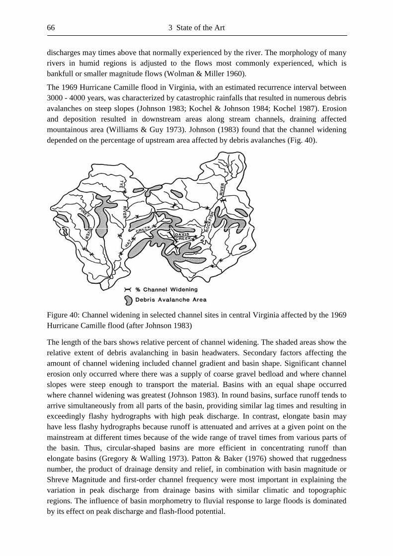
66 3 State of the Art

discharges may times above that normally experienced by the river. The morphology of many rivers in humid regions is adjusted to the flows most commonly experienced, which is bankfull or smaller magnitude flows (Wolman & Miller 1960).

The 1969 Hurricane Camille flood in Virginia, with an estimated recurrence interval between 3000 - 4000 years, was characterized by catastrophic rainfalls that resulted in numerous debris avalanches on steep slopes (Johnson 1983; Kochel & Johnson 1984; Kochel 1987). Erosion and deposition resulted in downstream areas along stream channels, draining affected mountainous area (Williams & Guy 1973). Johnson (1983) found that the channel widening depended on the percentage of upstream area affected by debris avalanches (Fig. 40).

Figure 40: Channel widening in selected channel sites in central Virginia affected by the 1969 Hurricane Camille flood (after Johnson 1983)

The length of the bars shows relative percent of channel widening. The shaded areas show the relative extent of debris avalanching in basin headwaters. Secondary factors affecting the amount of channel widening included channel gradient and basin shape. Significant channel erosion only occurred where there was a supply of coarse gravel bedload and where channel slopes were steep enough to transport the material. Basins with an equal shape occurred where channel widening was greatest (Johnson 1983). In round basins, surface runoff tends to arrive simultaneously from all parts of the basin, providing similar lag times and resulting in exceedingly flashy hydrographs with high peak discharge. In contrast, elongate basin may have less flashy hydrographs because runoff is attenuated and arrives at a given point on the mainstream at different times because of the wide range of travel times from various parts of the basin. Thus, circular-shaped basins are more efficient in concentrating runoff than elongate basins (Gregory & Walling 1973). Patton & Baker (1976) showed that ruggedness number, the product of drainage density and relief, in combination with basin magnitude or Shreve Magnitude and first-order channel frequency were most important in explaining the variation in peak discharge from drainage basins with similar climatic and topographic regions. The influence of basin morphometry to fluvial response to large floods is dominated by its effect on peak discharge and flash-flood potential.

3 State of the Art 67

Vegetation and soils can affect the flood response of a drainage basin. Generally, runoff and sediment yield declines with increasing vegetation density for a given rainfall intensity and duration (Langbein & Schumm 1958). Basins with thin soils tend to produce flashier floods with higher peak discharges for a given rainfall event than basins with thick soils. Within thick soils, once potential runoff water enters the subsurface system, large quantities of this infiltrated water may be temporarily bound in near-surface interflow or groundwater flow, so that the hydrograph peak occurs delayed and reduced.

River channel factors:

Channel, bank and floodplain erosion is favoured by high-velocity flows, carrying coarse bedload material that can be used as abrasive tools. Lithology, in combination with climate, largely controls the size of sediments delivered to channels from the drainage basin. Hack (1957) showed that channel gradient is affected by lithology for basins of similar size. Steep gradients generally occur in areas of resistant bedrock, while gentle gradients dominate in regions of weaker rocks. High channel gradients are required to efficiently transport coarse bedload delivered to channels in areas of resistant bedrock (Baker et al. 1988)

The effects of the Hurricane Camille flood in central Virginia in 1969 (Williams & Guy 1973) and a similar flood in western Virginia in 1949 (Hack & Goodlett 1960) differ strongly from the observations made of the Agnes flood, although all three floods occurred in a similar climatic regime (Coast 1974; Moss & Kochel 1978). The Pennsylvania and Maryland floods occurred in moderate-relief areas, where bedload was relatively fine grained, while the areas affected by floods in Virginia occurred in the high-relief areas, where bedload was dominated by coarse gravel and experienced upstream debris avalanching. Thus, extreme variability in fluvial response to floods can occur within the same climatic region. Extreme geomorphic response to flooding was reported for a number of studies that occurred in mountainous areas, where rivers have steep channel gradient and abundant coarse bedload, regardless of climate and vegetation (Stewart & LaMarche 1967; Scoot & Gravlee 1968; Baker 1977, 1984; Grozier et al. 1976; Costa 1978; Nolan & Marron 1985).

The geometry of stream channels plays an important role in determining the geomorphic effect of large floods. In terms of flood processes, bedrock and alluvial rivers can be considered as end members of the fluvial spectrum, characterized by different sediment yield and geomorphic work being done during large floods. Bedrock channels are common in uplifted plateau areas, especially in semi-arid and arid regions, usually have deep narrow cross-sections and are characterized by extremely increased flow depth and velocity during peak discharge. The 1954 extreme flood in Texas had an average flow depth greater than 25 m and average velocities of 12 m/s (Baker 1984).

Deep, high-gradient flood flows in bedrock channels usually result in macro-turbulent flow phenomena characterized by the birth and decay of vorticity around obstacles and along irregular channel boundaries (Baker 1984). Matthes (1947) described macro-turbulent phenomena, such as potholes, which are underwater vortexes that are created when rapidly rushing water passes an underwater obstacle in high shear boundary areas. Bedrock rivers with high velocity gradients produce violently rotating columns of water, which are capable of plucking multi-ton blocks of rock and transporting them in suspension for thousands of

68 3 State of the Art

meters. Baker (1977, 1978, 1984) described the intense upward vortex action developed when potholes are formed along irregular flow boundaries such as in the lee of bedrock protrusions, downstream of large boulders, and along irregular bedrock channel floors and walls. Potholes and other macro-turbulent flow phenomena such as cavitation may result in significant erosion of channel walls and floors during major floods. Baker (1978, 1984) described the dramatic effects of sedimentary deposits produced by bedrock river floods. Large volumes of coarse bedload are normally moved during bedrock river floods, and large-scale modification occurs on channel bars and floodplain areas. The resistance of bedrock channel walls is generally high enough to prevent significant change. Thus, the development of intensely energetic macro-turbulent flow phenomena occurs in these narrow, deep bedrock channels during floods. Baker (1977) in a study in Texas found that significant geomorphic changes only occur during rare large-magnitude floods, when macro-turbulent flow phenomena were established, and that subsequent floods of lower magnitude are unable to redistribute sediments. Thus, recovery of the landscape to pre-flood conditions is slow in semi-arid bedrock channels. In addition, the slow rate of vegetative re-establishment in arid regions prohibits rapid recovery (Wolman & Gerson 1978). In contrast, alluvial rivers in humid regions recover fast from changes of major floods. Localized channel scour and widening produced during Hurricane Agnes was masked by recovery within a few weeks to a year (Costa 1974; Gupta & Fox; Moss & Kochel 1978).

Beard (1975) mapped the United States according to its potential for flash flooding with a Flash-Flood Magnitude Index (FFMI), which describes the Qmax/Qmean ratio. The FFMI is a good measure for likelihood of streams to experience major geomorphic change during large floods. Baker (1977) noted that low FFMI values occur for extremely arid areas, suggesting that beside climatic factors, topography, vegetation and basin morphometry are important controls on flood response.

The complex interaction of variables important in controlling the channel response to large floods suggests that best insights into understanding these flood response controlling factors can be gained by comparing numerous studies where certain variables can be held constant. Systematic observations along a river that exhibits different gradient, sediment load, or channel geometry along its length would permit isolation of the effects of individual variables on geomorphic response to a flood (Baker et al. 1988).

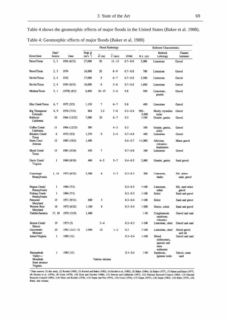
3 State of the Art 69

Table 4 shows the geomorphic effects of major floods in the United States (Baker et al. 1988). Table 4: Geomorphic effects of major floods (Baker et al. 1988)

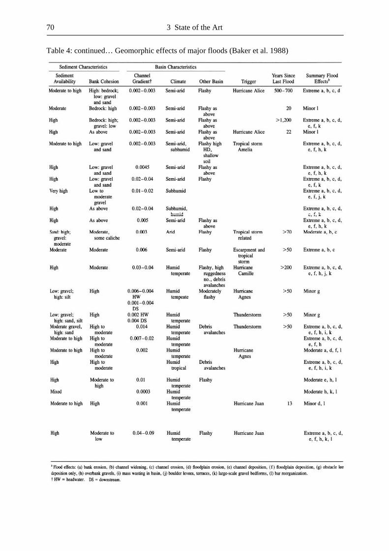
70 3 State of the Art

Table 4: continued… Geomorphic effects of major floods (Baker et al. 1988)

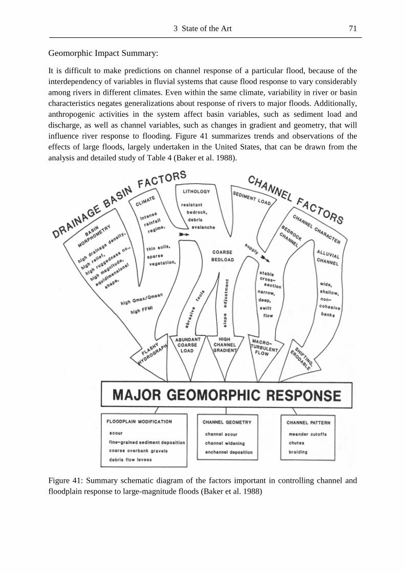
3 State of the Art 71

Geomorphic Impact Summary:

It is difficult to make predictions on channel response of a particular flood, because of the interdependency of variables in fluvial systems that cause flood response to vary considerably among rivers in different climates. Even within the same climate, variability in river or basin characteristics negates generalizations about response of rivers to major floods. Additionally, anthropogenic activities in the system affect basin variables, such as sediment load and discharge, as well as channel variables, such as changes in gradient and geometry, that will influence river response to flooding. Figure 41 summarizes trends and observations of the effects of large floods, largely undertaken in the United States, that can be drawn from the analysis and detailed study of Table 4 (Baker et al. 1988).

Figure 41: Summary schematic diagram of the factors important in controlling channel and floodplain response to large-magnitude floods (Baker et al. 1988)

72 3 State of the Art

Basin variables important in affecting fluvial geomorphic response to large floods include: climate, particularly the intensity-duration relationship for rainfall and the frequency of intense rainfall inputs into the system; river hydrology, particularly factors that relate to the flashiness of the hydrograph such as the portion of the basin contributing runoff to the mainstream and the peak discharge; basin morphometry, particularly factors that affect the flashiness of the mainstream hydrograph such as basin relief measures, drainage density, basin shape, vegetative cover and soil cover.

Streams that experience major geomorphic changes during large floods are characterized by: flashy hydrographs; high channel gradient; abundant coarse bedload; relatively low bank cohesion; channel cross-sections that enable flood discharges to be accompanied by deep, high velocity flows where macro-turbulent flow phenomena can be initiated and maintained. Flashy streams are most common in semi-arid and arid regions where intense, short-duration, local rainfalls are common, but intense rainfalls are also common in mountainous areas where orographic influences predominate in humid climates. Within these climatic zones where catastrophic rainfalls are common, rivers exhibit particularly flashy characteristics where drainage basin morphometry increases the rate and quantity of runoff delivered to the main channel.

Basin parameters likely to produce flashy conditions include: high relief, high drainage density, equal basin shape, high first-order stream frequency, high basin magnitude, sparse vegetation and thin soils. Factors coincident with streams showing dramatic response to floods but having less dependence on climate, because they are influenced by lithology and tectonics, are: high channel gradient, coarse bedload and channel geometry. Large quantities of coarse bedload are typical for channels that drain on resistant lithology. Thus, gradients are generally higher because the rivers adjust their slope to the load they have to transport. Therefore, during large floods on many streams, considerable geomorphic change occurs in headwater regions of high-gradient channels while minor response occurs downstream, where gradient and bedload availability are lower in spite of higher discharge (Moss & Kochel 1978).

Regions where dramatic channel response should be expected from large floods would be in mountainous basins of low stream order and/or in regions where recent tectonics has created high-gradient channels. These conditions may be independent of climate, although there would be a greater tendency for the production of coarse sediment in arid climates because of the reduced rate of soil production compared to humid regions of similar lithology.

Dramatic channel response to large floods occurs primarily when peak flood velocity and depth exceed threshold values necessary for the development and maintenance of macro-turbulence. These conditions result in exceedingly high values of unit stream power on the channel bed. Such conditions are most common in bedrock channels whose relatively stable cross-sections allow increase in discharge to be accompanied by dramatic increases in flow depth and velocity. Bedrock channels are not confined to a particular climatic regime but tend to be best developed in semi-arid to arid regions. Channels with this kind of geometry can better exceed competence levels required for the transportation of coarse bedload during major floods than ones that may adjust rapidly to increased discharges through channel widening.

3 State of the Art 73

In high relief areas such as first- and second-order basins, debris avalanches are important geomorphic processes, changing the drainage network system in a spectacular way. Debris avalanches can occur in all climatic regions and must be considered potential devastating natural hazards. In the United States floods account for one-fourth to one-third of the average annual dollar losses from geologic hazards and for 80 % of the annual loss of life from geologic hazards (Costa & Baker 1981). A tremendous cloudburst over the Serra das Araras escarpment in Rio de Janeiro, Brazil, triggered hundreds of debris avalanches and killed over 1000 people (Jones 1973). Williams & Guy (1973) reported that during the Hurricane Camille floods, 125 people died mainly as a consequence of their injuries caused by debris avalanches.

One of the first descriptions of debris avalanches was made by Cleland (1902). The debris avalanches on the slopes of Mt. Greylock, Massachusetts created chutes on the hillslopes ranging from 15 - 70 m width and up to 500 m length. The chutes were scoured to bedrock, forming new first-order channels, while eroded sediment was deposited as alluvial fans in adjacent lowlands. Hack & Goodlett (1960) studied the debris avalanches and chutes created during the June 1949 flood in the Little River basin in the Appalachian Mountains. Within this high-relief basin nearly 50 % of the drainage area consisted of small first-order basins, which are widely characterised by round hollows rimmed by steep slopes. The flood resulted from over 200 mm of rainfall and caused more than 100 landslides. Most of the chutes developed in slight runoff concentrating depressions on the hillslopes of first-order channels. Some of the about one meter deep chutes extended near to the slope crest and all extended to the base of the slope, intersecting with the channel. Six years after the flood event, the chutes still appeared quite fresh and unaltered compared to the older vegetated chutes. They concluded that the chutes represent the initiating stage of drainage extension by the creation of new hollows and new first-order streams. William & Guy (1973) found similar chutes and debris avalanches created during floods of Hurricane Camille in 1969 in the James River basin in Virginia, whereas chutes developed on the steepest slopes with a preferential N, NE or E aspect, indicating greater antecedent moisture conditions or wind-driven rainfall.

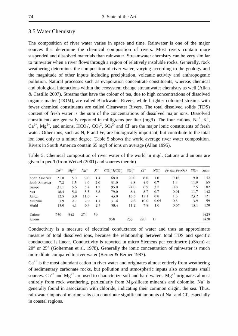
74 3 State of the Art

3.5 Water Chemistry

The composition of river water varies in space and time. Rainwater is one of the major sources that determine the chemical composition of rivers. Most rivers contain more suspended and dissolved materials than rainwater. Streamwater chemistry can be very similar to rainwater when a river flows through a region of relatively insoluble rocks. Generally, rock weathering determines the composition of river water, varying according to the geology and the magnitude of other inputs including precipitation, volcanic activity and anthropogenic pollution. Natural processes such as evaporation concentrate constituents, whereas chemical and biological interactions within the ecosystem change streamwater chemistry as well (Allan & Castillo 2007). Streams that have the colour of tea, due to high concentrations of dissolved organic matter (DOM), are called Blackwater Rivers, while brighter coloured streams with fewer chemical constituents are called Clearwater Rivers. The total dissolved solids (TDS) content of fresh water is the sum of the concentrations of dissolved major ions. Dissolved constituents are generally reported in milligrams per liter (mg/l). The four cations, Na+, K+, Ca2+, Mg2+, and anions, HCO3

-, CO32, SO4

2- and Cl- are the major ionic constituents of fresh water. Other ions, such as N, P and Fe, are biologically important, but contribute to the total ion load only to a minor degree. Table 5 shows the world average river water composition. Rivers in South America contain 65 mg/l of ions on average (Allan 1995).

Table 5: Chemical composition of river water of the world in mg/l. Cations and anions are given in µeq/l (from Wetzel (2001) and sources therein)

Conductivity is a measure of electrical conductance of water and thus an approximate measure of total dissolved ions, because the relationship between total TDS and specific conductance is linear. Conductivity is reported in micro Siemens per centimetre (µS/cm) at 20° or 25° (Golterman et al. 1978). Generally the ionic concentration of rainwater is much more dilute compared to river water (Berner & Berner 1987).

Ca2+ is the most abundant cation in river water and originates almost entirely from weathering of sedimentary carbonate rocks, but pollution and atmospheric inputs also constitute small sources. Ca2+ and Mg2+ are used to characterize soft and hard waters. Mg2+ originates almost entirely from rock weathering, particularly from Mg-silicate minerals and dolomite. Na+ is generally found in association with chloride, indicating their common origin, the sea. Thus, rain-water inputs of marine salts can contribute significant amounts of Na+ and Cl-, especially in coastal regions.

3 State of the Art 75

Pollution, due to domestic sewage, fertilizers and road salt are additional local sources, but most of the Na+ and Cl- constituents in natural streams originate from weathering of NaCl-containing rocks. Cl- is chemically and biologically inert and thus a useful tracer in nutrient experiments. K+ is the least abundant of the major cations in river water and originates mainly from the weathering of silicate materials, especially potassium feldspar and mica. SO4

2- has many sources, such as the weathering of sedimentary rocks, volcanic activity and pollution, through e.g. fertilizers, wastes and mining activities (Allan 1995). Na+, K+, Ca2+, Mg2+ and Cl- primarily derive from particles in the air, while SO4

2- and NO3- mainly derive from

atmospheric gases (Allan & Castillo 2007).

During stormflow, Avila et al. (1992) reported a decreased pH for a Mediterranean geo-ecosystem, Whitfield et al. (1993) for a maritime temperate forest environment and Elsenbeer et al. (1994) for a tropical ecosystem in Australia. During storm events, rainwater travels rapidly through macropores towards the stream and is thus more acid than the slower matrix flow, because of less equilibration time with the mineral soil (Neal et al. 1989; McDowell & Asbury 1994; McDowell 1998). Cl- concentrations can increase with discharge, due to Cl--rich precipitation (Mulder et al. 1990) or enrichment in the soil as a result of prolonged dry periods, associated with a high evapotranspiration (Avila et al. 1992). A dilution effect for Cl- during stormflow was found by Whitfield et al. (1993). Elsenbeer et al. (1994) observed a flushing effect of Cl- and SO4

2- during stormflow with an initial increase and a subsequent pronounced decrease of both anions.

In a variety of geo-ecosystems, the concentrations of Ca2+, Mg2+ and Na+ decrease during stormflow, while the concentration of K+ increases during stormflow. Thus, an increased K+ concentration during stormflow is an indicator of overland flow or ‘new’ water contribution. (Miller & Drever 1977; Feller & Kimmins 1979; Muscutt et al. 1990; Harriman et al. 1990; Avila et al. 1992; Hill 1993; Giusti & Neal 1993; Elsenbeer et al. 1994). The K+/SiO2 ratio is a useful measure to document this phenomena, since K+ is a characteristic tracer of fast flowpaths, being almost exclusively supplied by vegetation (Muscutt et al. 1990; Hill 1993; Elsenbeer et al. 1994), while SiO2 is a characteristic tracer of slow flowpaths and thus a indicator of ‘old’ water, which is almost exclusively supplied by the weathering zone. As vegetation mainly interacts with near-surface rapid flow paths in response to rainfall, the high K+/SiO2 ratio at La Cuenca, Peru indicates the contribution of fast flowpaths (Elsenbeer et al. 1995b). However, while ‘new’ water contribution implies fast pathways, such as overland flow, ‘old’ water contribution is not necessarily associated with slow pathways in responsive forested catchments, characterized by fast flowpaths (Bonell & Gilmour 1978; McDonnell 1990). At South Creek in tropical Australia, fast pathways supply ‘old’ and ‘new’ water to the streams (Elsenbeer et al. 1994).

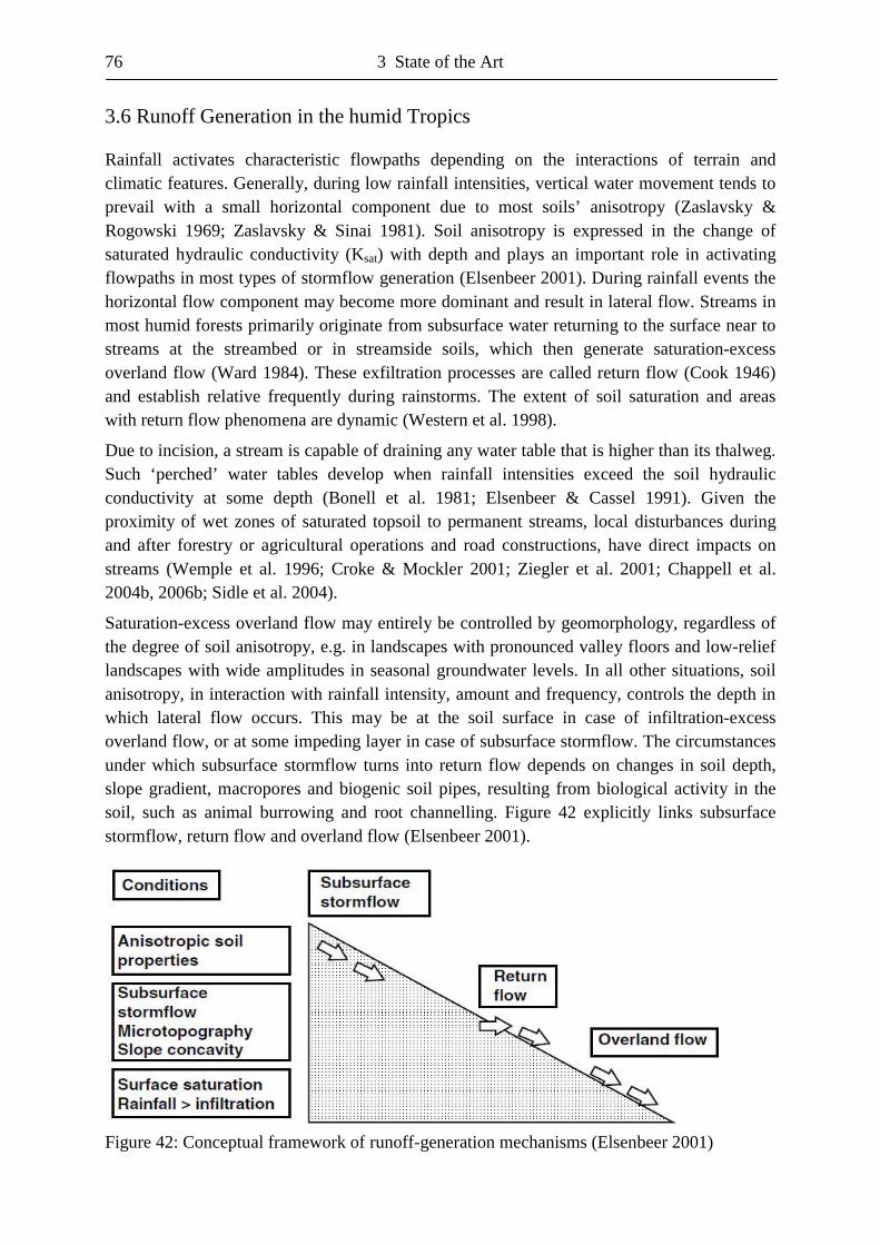
76 3 State of the Art

3.6 Runoff Generation in the humid Tropics

Rainfall activates characteristic flowpaths depending on the interactions of terrain and climatic features. Generally, during low rainfall intensities, vertical water movement tends to prevail with a small horizontal component due to most soils’ anisotropy (Zaslavsky & Rogowski 1969; Zaslavsky & Sinai 1981). Soil anisotropy is expressed in the change of saturated hydraulic conductivity (Ksat) with depth and plays an important role in activating flowpaths in most types of stormflow generation (Elsenbeer 2001). During rainfall events the horizontal flow component may become more dominant and result in lateral flow. Streams in most humid forests primarily originate from subsurface water returning to the surface near to streams at the streambed or in streamside soils, which then generate saturation-excess overland flow (Ward 1984). These exfiltration processes are called return flow (Cook 1946) and establish relative frequently during rainstorms. The extent of soil saturation and areas with return flow phenomena are dynamic (Western et al. 1998).

Due to incision, a stream is capable of draining any water table that is higher than its thalweg. Such ‘perched’ water tables develop when rainfall intensities exceed the soil hydraulic conductivity at some depth (Bonell et al. 1981; Elsenbeer & Cassel 1991). Given the proximity of wet zones of saturated topsoil to permanent streams, local disturbances during and after forestry or agricultural operations and road constructions, have direct impacts on streams (Wemple et al. 1996; Croke & Mockler 2001; Ziegler et al. 2001; Chappell et al. 2004b, 2006b; Sidle et al. 2004).

Saturation-excess overland flow may entirely be controlled by geomorphology, regardless of the degree of soil anisotropy, e.g. in landscapes with pronounced valley floors and low-relief landscapes with wide amplitudes in seasonal groundwater levels. In all other situations, soil anisotropy, in interaction with rainfall intensity, amount and frequency, controls the depth in which lateral flow occurs. This may be at the soil surface in case of infiltration-excess overland flow, or at some impeding layer in case of subsurface stormflow. The circumstances under which subsurface stormflow turns into return flow depends on changes in soil depth, slope gradient, macropores and biogenic soil pipes, resulting from biological activity in the soil, such as animal burrowing and root channelling. Figure 42 explicitly links subsurface stormflow, return flow and overland flow (Elsenbeer 2001).

Figure 42: Conceptual framework of runoff-generation mechanisms (Elsenbeer 2001)

3 State of the Art 77

The generation of overland flow by pipe outlets on hillslopes was first observed during several events in the highly responsive tropical rainforest catchment La Cuenca, Peru in western Amazonia (Elsenbeer & Cassel 1990, 1991). At La Cuenca, the chemical signature of fast flow paths is distinct from that of slow flow paths. Overland flow, occurring in any season, dominates the stormflow hydrograph during high-intensity events. Antecedent soil moisture conditions only influence the volumes generated. During low-intensity events and base flow conditions, the groundwater chemical signal is dominant. Given that overland flow in many places is generated by pipe flow, the chemical distinction between the two is complex (Elsenbeer & Lack 1996a).

From the catchment point of view, the distinction between pipe flow and overland flow is meaningless. There is one fast flowpath, being neither entirely at the soil surface nor entirely below it, and one slow flowpath, being significantly different in its hydrochemical composition, due to its longer contact time in the ecosystem (Elsenbeer et al. 1995b). To avoid the exclusive subsurface and surface connotation of pipe flow, often being classified as subsurface stormflow, and overland flow, respectively, the term return flow (Kirkby 1988) is more appropriate, because it captures the origin of overland flow, while acknowledging the existence of pipe flow (Elsenbeer et al. 1995b).

Overland flow is a mixture of subsurface sources or pre-event water, originating from hillslope groundwater and soil water, and surface sources or event water, depending on hydrometeorological features, antecedent soil moisture conditions and the degree of incision of individual flow lines (Elsenbeer & Lack 1996a). Hydraulic properties of permeability, including moisture release characteristics, porosity and dispersivity act as a major control on the flow vectors. Many hillslopes contain systems of preferential flow channels known as macropores or natural soil pipes (Beven & Germann 1982; Jones 1990). Active soil pipes have their greatest effect on subsurface stormflow under very wet catchment conditions, when the threshold for pipeflow initiation might be exceeded in many locations (Gilman & Newson 1980). In the Baru catchment, Malaysia, rainstorms with a daily rainfall volume of 50 - 100 mm, activate natural soil pipes with diameters between 0.01 and 0.5 m, returning water to the surface (Chappell et al. 1998). Soil piping in Acrisol-Alisol soils has been reported in Sarawak, Malaysia (Baillie 1975), Singapore (Sherlock et al. 1995) and Peru (Elsenbeer & Lack 1996a). Such studies indicate that pipe flow is a dominant pathway in tropical regions, transferring water to the streams. Thus, small-scale measurements of the permeability of soils in between these discrete preferential pathways may underestimate the ‘block permeability’ of hillslope-sized soil unit (Wen & Gómez-Hernández 1996). Direct characterization of larger soil blocks as a single unit, about the size of a whole hillslope, may be a way to include the effects of pipe flow systems (Jones 1990; Chappell & Ternan 1992; Bonell & Balek 1993).

The Amazon basin contains the largest continuous area of tropical rainforest, covering an area of more than 7 million km2 (Sioli 1984). The continental scale of the Amazon River basin comprises a considerable lithological and geomorphological diversity. The rich land- and soilscape reflects the geological history of the Amazon basin (Klammer 1984). Because hydrological processes significantly are controlled by properties of the soil such as the change of hydraulic conductivity with depth (Dunne 1983), soilscape diversity in the Amazon basin gives rise to various hillslope and catchment hydrological response patterns.

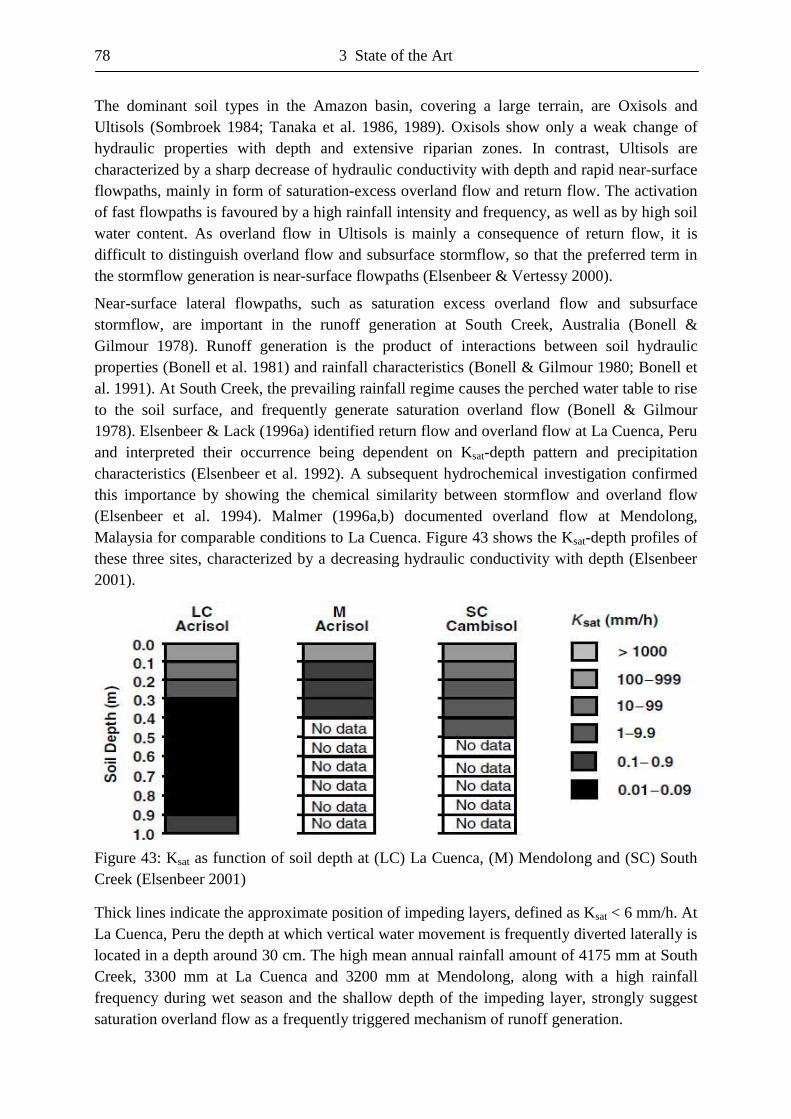
78 3 State of the Art

The dominant soil types in the Amazon basin, covering a large terrain, are Oxisols and Ultisols (Sombroek 1984; Tanaka et al. 1986, 1989). Oxisols show only a weak change of hydraulic properties with depth and extensive riparian zones. In contrast, Ultisols are characterized by a sharp decrease of hydraulic conductivity with depth and rapid near-surface flowpaths, mainly in form of saturation-excess overland flow and return flow. The activation of fast flowpaths is favoured by a high rainfall intensity and frequency, as well as by high soil water content. As overland flow in Ultisols is mainly a consequence of return flow, it is difficult to distinguish overland flow and subsurface stormflow, so that the preferred term in the stormflow generation is near-surface flowpaths (Elsenbeer & Vertessy 2000).

Near-surface lateral flowpaths, such as saturation excess overland flow and subsurface stormflow, are important in the runoff generation at South Creek, Australia (Bonell & Gilmour 1978). Runoff generation is the product of interactions between soil hydraulic properties (Bonell et al. 1981) and rainfall characteristics (Bonell & Gilmour 1980; Bonell et al. 1991). At South Creek, the prevailing rainfall regime causes the perched water table to rise to the soil surface, and frequently generate saturation overland flow (Bonell & Gilmour 1978). Elsenbeer & Lack (1996a) identified return flow and overland flow at La Cuenca, Peru and interpreted their occurrence being dependent on Ksat-depth pattern and precipitation characteristics (Elsenbeer et al. 1992). A subsequent hydrochemical investigation confirmed this importance by showing the chemical similarity between stormflow and overland flow (Elsenbeer et al. 1994). Malmer (1996a,b) documented overland flow at Mendolong, Malaysia for comparable conditions to La Cuenca. Figure 43 shows the Ksat-depth profiles of these three sites, characterized by a decreasing hydraulic conductivity with depth (Elsenbeer 2001).

Figure 43: Ksat as function of soil depth at (LC) La Cuenca, (M) Mendolong and (SC) South Creek (Elsenbeer 2001)

Thick lines indicate the approximate position of impeding layers, defined as Ksat < 6 mm/h. At La Cuenca, Peru the depth at which vertical water movement is frequently diverted laterally is located in a depth around 30 cm. The high mean annual rainfall amount of 4175 mm at South Creek, 3300 mm at La Cuenca and 3200 mm at Mendolong, along with a high rainfall frequency during wet season and the shallow depth of the impeding layer, strongly suggest saturation overland flow as a frequently triggered mechanism of runoff generation.

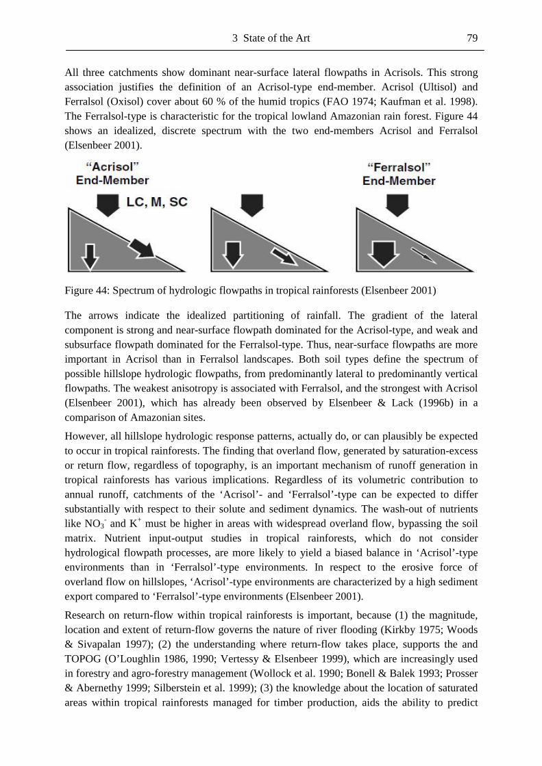
3 State of the Art 79

All three catchments show dominant near-surface lateral flowpaths in Acrisols. This strong association justifies the definition of an Acrisol-type end-member. Acrisol (Ultisol) and Ferralsol (Oxisol) cover about 60 % of the humid tropics (FAO 1974; Kaufman et al. 1998). The Ferralsol-type is characteristic for the tropical lowland Amazonian rain forest. Figure 44 shows an idealized, discrete spectrum with the two end-members Acrisol and Ferralsol (Elsenbeer 2001).

Figure 44: Spectrum of hydrologic flowpaths in tropical rainforests (Elsenbeer 2001) The arrows indicate the idealized partitioning of rainfall. The gradient of the lateral component is strong and near-surface flowpath dominated for the Acrisol-type, and weak and subsurface flowpath dominated for the Ferralsol-type. Thus, near-surface flowpaths are more important in Acrisol than in Ferralsol landscapes. Both soil types define the spectrum of possible hillslope hydrologic flowpaths, from predominantly lateral to predominantly vertical flowpaths. The weakest anisotropy is associated with Ferralsol, and the strongest with Acrisol (Elsenbeer 2001), which has already been observed by Elsenbeer & Lack (1996b) in a comparison of Amazonian sites.

However, all hillslope hydrologic response patterns, actually do, or can plausibly be expected to occur in tropical rainforests. The finding that overland flow, generated by saturation-excess or return flow, regardless of topography, is an important mechanism of runoff generation in tropical rainforests has various implications. Regardless of its volumetric contribution to annual runoff, catchments of the ‘Acrisol’- and ‘Ferralsol’-type can be expected to differ substantially with respect to their solute and sediment dynamics. The wash-out of nutrients like NO3

- and K+ must be higher in areas with widespread overland flow, bypassing the soil matrix. Nutrient input-output studies in tropical rainforests, which do not consider hydrological flowpath processes, are more likely to yield a biased balance in ‘Acrisol’-type environments than in ‘Ferralsol’-type environments. In respect to the erosive force of overland flow on hillslopes, ‘Acrisol’-type environments are characterized by a high sediment export compared to ‘Ferralsol’-type environments (Elsenbeer 2001).

Research on return-flow within tropical rainforests is important, because (1) the magnitude, location and extent of return-flow governs the nature of river flooding (Kirkby 1975; Woods & Sivapalan 1997); (2) the understanding where return-flow takes place, supports the and TOPOG (O’Loughlin 1986, 1990; Vertessy & Elsenbeer 1999), which are increasingly used in forestry and agro-forestry management (Wollock et al. 1990; Bonell & Balek 1993; Prosser & Abernethy 1999; Silberstein et al. 1999); (3) the knowledge about the location of saturated areas within tropical rainforests managed for timber production, aids the ability to predict

80 3 State of the Art

local sensitivity to soil disturbance and thus areas to focus protective measures (Chappell et al. 2006b) and (4) tropical forestry has a significant impact on erosion and the general behaviour of a river. Yet there’s a lack of studies of sediment and nutrient losses and flow-pathways in both managed and undisturbed tropical rainforests. Thus, generalisations about the amount of near-surface water flowpaths in natural rainforest slopes and on skid trails are highly uncertain (Tangtham 1994; Bonell 2004; Chappell et al. 2004c Chappell & Sherlock 2005; Chappell et al. 2006b).

Under the assumption of saturation-excess as the prevailing mechanism for the generation of overland flow, high frequencies are expected for steep slopes (Chappell et al. 2006b). However, at La Cuenca, Peru, pipe outlets are responsible for the high frequency of overland flow. Hydrological discontinuities lead to return flow and surface saturation, so that overland flow and subsurface stormflow are closely linked in many places (Elsenbeer & Vertessy 2000). Chappell et al. (1998, 1999a,b, 2004b) suggest that high pore water pressure-waves and natural soil pipes, rather than saturation overland flow, are important mechanisms to explain the fast stream response during rainstorm events within humid tropical environments.

For the Baru catchment in Malaysia it was shown that, even during large storms, the topsoil in all but valley bottom or channel head areas remained less than saturated (Sherlock 1997; Chappell & Sherlock 2005). The same phenomenon was observed within granite catchments in Singapore Island (Sherlock et al. 1995, 2000) and Peninsular Malaysia (Noguchi et al. 1997). These catchments are usually not associated with cyclonic storms that may produce extensive topsoil saturation (Bonell et al. 1981, 2004). Soil moisture observations within Huai Pacha and a nearby agricultural catchment in Thailand showed that most of the topsoil is relatively dry only a few hours after a storm in the wet season (Vongtanaboon 2004). Thus, tropical catchments in non-cyclonic regions may produce very fast stream responses without extensive topsoil saturation (Bidin & Greer 1997; Chappell et al. 1999a). Tropical forestry impacts in the humid tropics:

The greatest potential hydrological and pedological impacts and disturbances within commercial managed natural tropical rainforests along perennial streams results from ground skidding, from haulage road construction, from tracks and wheels of forestry vehicles and from logs that are hauled behind the skidder (Chappell et al. 2004c). Forestry vehicles, skid trails and haulage roads locally compact the topsoil, reduce its hydraulic permeability (Van der Plas & Bruijnzeel 1993; Malmer 1996) and increase the likelihood of infiltration-excess (Horton 1933) and saturation-excess overland flow being generated (Baharuddin 1995; Douglas et al. 1995; Ziegler et al. 2001; Chappell et al. 2004a,b). Thus a common phenomenon is infiltration-excess overland flow water running on predetermined road pathways towards undisturbed slopes. When the sediment laden water infiltrates into the soil its deposits accumulate upon the slope (Chappell et al. 2004b; Sidle et al. 2004). As forestry roads are normally constructed parallel to the slope, they must cross the streams. At these crossing, the surface hydraulic connection between slopes and permanent channels can be increased. The resulting overland flow can shed water and any carried sediments or chemicals into the stream.

3 State of the Art 81

Hydrological buffer zones in the humid tropics:

It is important to protect sensitive wet streamside soils and material contributing upslope areas for the following reasons (Chappell et al. 2006b). Wet stream-side soils have lower shear strengths and are more erosive than drier soils (Bryan 2000). Therefore they are more sensitive to mechanical damage and disturbance by forestry vehicles. As a consequence, the likelihood that sediments and nutrients reach the stream is increased. Saturated soils with fast overland flow near to stream channels can contribute a great amount of eroded and mobilised sediments and nutrients from upslope areas to the stream. As a consequence, local or downstream fauna can be damaged. Corridors of undisturbed native trees along stream banks maintain the natural stream temperature due to their shadow contributing crowns and thereby sustain fish habitats (Pusey & Arthington 2003). Additionally, these trees help to maintain the seed-pool, which allows the regeneration of selectively logged forest on adjacent slopes, as well as easier migration of ground and canopy dwelling fauna (Laurance & Laurance 1999).

Thus, a better understanding of the return-flow patterns and processes within tropical rainforests is needed (Woods & Sivapalan 1997; Bonell 2004). Research and visual observations in South East Asian tropical forests like in East Malaysia (Baru), Singapore (Bukit Timah), Brunei (Mata Ikan) and Thailand (Huai Pacha, Huai Daf and Kog Ma) support the idea that most rainfall infiltrates into the soil, flows toward the stream channels and re-emerges in the channel bed, banks or soils adjacent to the stream (Sherlock et al. 1995; Sherlock 1997; Chappell et al. 1998, 1999a, 1999b, 2004a, 2004b; Franks et al. 1997; Vongtanaboon 2004; Chappell & Sherlock 2005).

Chappell et al. (2006b) showed for the Baru catchment that wet soils coincide with areas of high topographic convergence and values of the spatial distribution greater than 9 ln(m), indicating that topography exerts a strong influence on the location of return-flow and the pattern of soil moisture content. The comparison of the perennial channel head locations with threshold values of spatial distribution indicate that the Kirkby topographic index is a useful in locating the perennial stream network on digital maps for objective ‘hydrological buffer zones’, defining smaller zones with a higher proportion of sensitive wet soils. Hence, the -based buffers would be more efficient, easier to justify and allow access to more of the timber growing on less sensitive drier soils. Obviously, the use of such an index, which identifies buffer zones on all streams from an ecological point of view, is more acceptable than the current common practice of only defining buffer zones along streams wider than 5 m (Cassells et al. 1984; Sist et al. 1998; Chappell et al. 2006b).

If infiltration-excess overland flow is not significant within a catchment (Bonell 2004), the protection of wet zones may be considered sufficient for surface hydrological buffering, but the lateral extent of soil saturation may be relatively stationary or very dynamic, changing significantly through storm periods (Anderson & Kneale 1980). Given that extreme storms with a 10-year or even 100-year return period have a much greater impact on erosion, mass movement and sediment transport, this definition might be problematic (Douglas et al. 1999; Chappell et al. 2004c). However, the suggestion, to use 10-year or even 100-year storm return periods to map and define the minimum size of ‘hydrological buffer zones’ is rather impractical, as it is often difficult to access rain forest terrain during such large events (Chappell et al. 2006b).

82 3 State of the Art

3.7 Climate Change

Considering global warming impacts on South America, changes in extremes, negative trends for cold nights and positive trends for warm nights, intense rainfall events and consecutive dry days are expected. During the 20th century, significant increases in precipitation were observed in Southern Brazil, Paraguay, Uruguay, North-east Argentina, North-west Peru and Ecuador. In contrast, a declining trend in precipitation was observed in Southern Chile, South-west Argentina and Southern Peru. In Ecuador from 1930 - 1990 temperatures increased between 0.08 - 0.27 °C every 10 years. The glacier-retreat trend has reached critical conditions in Bolivia, Peru, Colombia and Ecuador, where water availability has already declined either for consumption, irrigation or hydropower generation. Within the next decades Andean inter-tropical glaciers are very likely to disappear and will thus affect water availability and hydropower generation. Water supply problems are expected to increase in future and become chronic if no appropriate adaptation measures are planned and implemented (ICCP 2007). In Ecuador, there has been a gradual decline in glacier length and water supply for irrigation and hydroelectric power plants as well as clean water supply for Quito has decreased (Magrin et al. 2007). Recent studies indicate that 7 of 11 principal basins in Ecuador would be affected by a decreasing annual runoff and therefore result in periods of water shortage (Cáceres 2004).

During the last 10 - 20 years the rate of sea-level rise has increased from 1 to 2 - 3 mm/yr in SE South America. In the future, unfavourable impacts might affect the mangroves in e.g. Ecuador, Brazil, Colombia and Venezuela. In particular, sea-level rise is very likely to affect both Mesoamerican coral reefs, e.g. in Mexico, Belize and Panama, and the location of fish stocks in the SE Pacific, e.g. Ecuador, Peru and Chile. Low-lying coasts in several Latin American countries like Ecuador are among the most vulnerable to climate change and extreme hydrometeorological events such as rainstorms, windstorms and sub-tropical and tropical cyclones and associated storm surges (ICCP 2007).

In the scenario of a 38 - 104 cm sea-level rise, mangrove areas could disappear from exposed and marginal environments, whereas the greatest changes would occur in the high-sedimentation, high-tide and drowned river-valley environments. A shrimp farm area of 1204 km2 would be affected, with a consequent decrease in production and economic gain (Medina et al. 2001). Protection measures in the form of coastal defence of the Guayas river delta would cost less than 2 billion US-Dollars. The benefits are supposed to be two or three times higher than the investment into protection measures. Reforestation of mangroves and preservation of flooded areas in Ecuador should be of primary interest in respect to ecology, economy and sociology (NC-Ecuador 2000).

On a larger scale, a higher energy input enhances the hydrological cycle and may increase precipitation and evapotranspiration. Glacier melt and an upward shift of the snowline affect discharge rates and timing (Foster 2001; IPCC 2001; Meybeck 2004). Due to the difficult monitoring circumstances, complex topography, vegetation and soils and the rapid spatial and temporal changes in climatic parameters, there is a relative scarcity of long range datasets that limit the knowledge of runoff generation in mountain areas, especially in the tropics and the subtropics (Beniston 2003; Meybeck et al. 2005).

3 State of the Art 83

Compared to the whole drainage basin, mountainous regions provide a rich, reliable and low variable water contribution to rivers, which is important for the ecology, the economy and the water supply for human consumption, most notably, agricultural use and hydroelectric power plants (Buytaert et al. 2006). About 40 % of the global population live in watersheds of rivers originating in sensitive and vulnerable montane ecosystems (Beniston 2003). In many locations, human land use has changed these natural landscapes, through ecological and geomorphological deterioration, leading to the loss of habitats and a declining biodiversity, as well as to increased erosion. Such land use changes might also have an impact on the water cycle. Changes in soil properties, vegetation, land cover and land management alter the water regulation capacity of mountainous catchments in different ways (Buytaert et al. 2006).

Global climate change is expected to have a strong impact on water resources (Huntington 2006; IPCC 2007). Changes in precipitation affect water availability and runoff directly, while changes in temperature, radiation and humidity influence evapotranspiration. There is social-economic need to predict the potential effects of climate change on the timing and magnitude of a steams’ discharge (Vergara et al. 2007). The study of Buytaert et al. (2009) analysed the impact of uncertainties related to global circulation model projections on future changes of streamflow in the Paute river basin, Ecuador. Although uncertainties in the hydrological model and downscaling techniques are neglected, prediction ranges are wide and of the same magnitude as current discharges.

Tropical forests play a major role in regulating the earth’s climate and hydrological cycles. Thus, tropical deforestation is widely believed to influence local, regional and global climate, because the trees of the humid tropics provide water vapour through evapotranspiration (Sagan et al. 1979; Salati & Nobre 1991). Although the relationship between deforestation and climate change is complex, there is a growing consensus that deforestation leads to warmer and drier climates. However, these model-based simulations of the effects of deforestation on climate are analytical experiments. They are not intended to be predictions of the impacts of contemporary deforestation. For one thing, the models assume that forests are removed instantaneously and completely. This assumption is contrary to most real-world situations, where deforestation is a gradual and fragmented process. In addition, growing secondary forests are not taken into account. In reality, the regrowth could compensate the impacts of deforestation. These factors alone suggest that the climatic impacts of contemporary deforestation are unlikely to be as dramatic or as clear as the model results might suggest. There is an urgent need for analyses based on real-world data and situations in tropical areas. Such studies should evaluate the quantity and spatial distribution of deforestation, as well as the quality of the climate record. Climatic trends should be examined in the context of large-scale climate changes or variability, such as global warming or El Niño, so that they are not mistakenly attributed to deforestation. More studies, considering deforestation and climate change on the local and regional scale could contribute to a better understanding of the complex nature of atmosphere-biosphere interactions. Without suchlike studies, possible impacts of deforestation on local and regional climates will continue to be based on the results of micro-scale studies and global modeling experiments. Hence, the question, whether the same processes are significant at all scales remains an unresolved question (O’Brien 1996).

84 3 State of the Art

3.8 Paleoflood Hydrology

Paleoflood hydrology uses geological evidences for the reconstruction of the magnitude and frequency of recent, past or ancient floods (Baker et al. 2002). Most ungauged basins studies research the last 5.000 years with an emphasis on the last millennium and century. Paleoflood hydrology is not defined by the time of flooding, but by the fact that flood evidence is derived from lasting physical effects on natural indicators (Benito & Thorndycraft 2005).

J. Harlem Bretz made the first paleohydrologic discharge estimates by using the Chezy equation, which is developed for uniform flow (Bretz 1929; Bretz et al. 1956). Hydraulic descriptions of non-uniform flow improved paleoflood discharge estimates (Baker 1973; Baker et al. 1979; Patton et al. 1979; Kochel et al. 1982). The most important formula is the slope-area method of peak discharge estimation described by Dalrymple & Benson (1967). This procedure can be applied to reaches of steady, gradually varied flow where multiple sites of high-water indicators exist. The method represents an improvement over the direct use of the Chezy and Manning equations in that it does, within limits, account for flow energy losses associated with variations in channel geometry and roughness along a stream reach. Although sound in principle and widely used, the slope-area method produces estimates that are relatively high compared to direct discharge measurements (Jarrett 1984) or more variable than discharges calculated by using more sophisticated hydraulic-modeling techniques (Webb 1985).

The term and concepts of paleoflood hydrology were introduced by Kochel & Baker (1982). The most accurate paleoflood technique is based on the identification of high-water marks and paleostage indicators (PSIs), such as slackwater sediments, debris accumulations, silt and scour lines, high-flow channels as well as other high-water marks such as drift wood and damage to vegetation. These paleoflood indicators can be correlated to define the paleoflood water surface profiles along river channels. Studies of prehistoric floods have proven to be effective in determining flood frequency and magnitude relationships for certain types of fluvial systems by using geologic evidence for paleoflood stages (Baker et al. 1979, 1983; Patton et al. 1979; Kochel et al. 1982; O’Connor et al. 1986). Hydraulic computations using either one- or two-dimensional hydraulic models can provide a good estimation of the discharges associated with the PSIs (O’Connor & Webb 1988; Webb & Jarrett 2002; Denlinger et al. 2002). Together with absolute age dating, flood magnitude and frequency over long time spans can be reconstructed (Benito & Thorndycraft 2005).

In order to lengthen flood records beyond instrumental gauging station data, paleoflood hydrology has been successfully applied in many regions of the world: USA (Kochel et al. 1982; Ely & Baker 1985; O’Connor et al. 1994), Australia (Baker & Pickup 1987; Pickup et al. 1988), India (Ely et al. 1996; Kale et al. 2000), Israel (Greenbaum et al. 2000); Spain (Benito et al. 2003a; Benito & Thorndycraft 2004; Thorndycraft et al. 2005), France (Sheffer et al. 2003a), Greece (Woodward et al. 2001), South Africa (Zawada 1997), China (Yang et al. 2000) and Japan (Jones et al. 2001).

3 State of the Art 85

Paleoflood hydrology is an inter-disciplinary research field that particularly incorporates geomorphology, sedimentology, hydrology, hydraulic modeling and statistics. Paleoflood analysis studies include various methodological approaches, such as (1) interpretation of variable scale aerial photos and topographic maps to identify suitable sites for paleoflood hydrological research; (2) field study and survey for the identification and selection of flood indicators such as flood deposits and high-water marks; (3) stratigraphical description with emphasis on identifying the number of flood units in a given sedimentary sequence; (4) sample collection for age dating of the flood deposits; (5) topographic survey of flood sites and river reaches; (6) hydraulic calculations and discharge estimation; (7) comparison with available historical and instrumental flood data; and (8) flood frequency analysis, as recurrence intervals of rare floods are often too long to be accurately assessed by using standard hydrologic engineering practices (Baker 1987; Benito & Thorndycraft 2005). Slackwater Deposits Analysis:

The most commonly utilised paleostage indicators (PSIs) in paleoflood hydrology are slackwater flood deposits (Baker 1987). These deposits accumulate in stable bedrock canyons at sites away from the main channel flow, where during high floods, eddies, back-flooding and water stagnation occur. These hydrological phenomena significantly reduce flow velocity and result in the deposition of clay, silt and sand (Baker & Kochel 1988; Benito et al. 2003b).

Paleoflood sites are controlled by a sediment source or the presence of fine-grained sediments in the catchment and according conditions of preservation. A catchment geology dominated by granite- or sandstones provides an abundant source of fine-grained material to be transported as suspended sediment during flood events. The deposition and preservation conditions during floods are controlled by the interplay between erosion and sedimentation processes and, afterwards, by post-flood erosion processes such as slope- and tributary runoff. Ideal conditions for the preservation of slackwater paleoflood deposits are given when sediments are deposited in valley side caves, alcoves or rock overhangs, where they are protected from erosion, slope movements, bioturbation and colonisation of flora and fauna after the flood event (Sheffer et al. 2003a; Thorndycraft et al. 2005). Tributary mouths and transitional reaches with abrupt canyon narrowing or widening are also suitable sites for flood deposits (Kochel et al. 1982; Kochel & Baker 1988). Depositional landforms in such environments include thick high-standing terraces. However, in marginal channel zones with the development of eddies during floods stages, flood deposits may be reformed, preserving a ridge morphology more typical of eddy bars (Ely & Baker 1985).

Slackwater terraces are developed by standing or slow-moving water that allows a better preservation of flood deposits through time (Patton et al. 1979; Kochel et al. 1982; Ely & Baker 1985; Benito et al. 2003a). Layers of sedimentary units of slackwater flood sediments may be deposited by successive flood events over long periods, building up sediment profiles. If the preservation of flood deposits at a particular site is good, the number of floods can be identified in the sedimentary profile (Benito & Thorndycraft 2005).

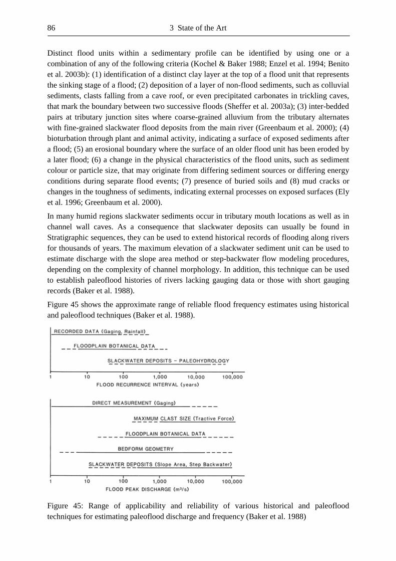
86 3 State of the Art

Distinct flood units within a sedimentary profile can be identified by using one or a combination of any of the following criteria (Kochel & Baker 1988; Enzel et al. 1994; Benito et al. 2003b): (1) identification of a distinct clay layer at the top of a flood unit that represents the sinking stage of a flood; (2) deposition of a layer of non-flood sediments, such as colluvial sediments, clasts falling from a cave roof, or even precipitated carbonates in trickling caves, that mark the boundary between two successive floods (Sheffer et al. 2003a); (3) inter-bedded pairs at tributary junction sites where coarse-grained alluvium from the tributary alternates with fine-grained slackwater flood deposits from the main river (Greenbaum et al. 2000); (4) bioturbation through plant and animal activity, indicating a surface of exposed sediments after a flood; (5) an erosional boundary where the surface of an older flood unit has been eroded by a later flood; (6) a change in the physical characteristics of the flood units, such as sediment colour or particle size, that may originate from differing sediment sources or differing energy conditions during separate flood events; (7) presence of buried soils and (8) mud cracks or changes in the toughness of sediments, indicating external processes on exposed surfaces (Ely et al. 1996; Greenbaum et al. 2000).

In many humid regions slackwater sediments occur in tributary mouth locations as well as in channel wall caves. As a consequence that slackwater deposits can usually be found in Stratigraphic sequences, they can be used to extend historical records of flooding along rivers for thousands of years. The maximum elevation of a slackwater sediment unit can be used to estimate discharge with the slope area method or step-backwater flow modeling procedures, depending on the complexity of channel morphology. In addition, this technique can be used to establish paleoflood histories of rivers lacking gauging data or those with short gauging records (Baker et al. 1988).

Figure 45 shows the approximate range of reliable flood frequency estimates using historical and paleoflood techniques (Baker et al. 1988).

Figure 45: Range of applicability and reliability of various historical and paleoflood techniques for estimating paleoflood discharge and frequency (Baker et al. 1988)

3 State of the Art 87

Slackwater paleoflood techniques can provide estimates of the discharge and frequency of large floods over greater temporal ranges than other methods. In addition, the slackwater technique can be used to estimate discharges of large floods and obtain continuous records over hundreds to thousands of years. Although paleohydrologic estimates contain some error, they provide excellent order-of-magnitude estimates of the frequency and magnitude of expected river discharges. In addition, paleohydrologic investigations such as the slackwater technique can be done rapidly and inexpensively compared to the costs of constructing major flood control structures. Standard statistical hydrological techniques of estimating the frequency of rare, large-magnitude floods become increasingly unreliable as the recurrence interval of the flood exceeds the length of historical gauging records (Baker et al. 1988). The water levels associated with different paleostages can be converted into flood discharge, which is the random variable used in statistical analysis (Francés 2004). Most calculated discharges from slackwater flood deposits are minimum discharge values, because the water depth above the specific flood deposits is unknown, but there are many ways to estimate past flood discharge from a known water surface elevation (O’Connor & Webb 1988, Webb & Jarrett 2002; Kutija 2003). In the majority of cases they assume one-dimensional flow based on slope-conveyance, slope-area, step-backwater and critical-depth methods. These models assume a fixed bed of stable bedrock. Data required include channel slope, roughness, which is usually Manning’s n, cross-sectional geometry and, for the step-backwater method, a boundary condition (Benito & Throndycraft 2005).

The two principal sources of error are an underestimation of paleo-discharge, due to the unknown level of the floodwaters above the deposited sediments, and changes in the valley cross-section (Benito & Thorndycraft 2005). The first error can be approached by studies of the sedimentology of the flood deposits that enable interpretations regarding flow velocities and energy conditions at the site of deposition. Therefore, inferences can be made regarding the level of the water above the deposits (Benito et al. 2003b; Thorndycraft et al. 2005). The second error, concerning cross-sectional stability, is limited, due to the lack of paleoflood studies about bedrock gorge reaches. Bedrock channel geometry is significantly more stable than alluvial floodplain channels and will not have been substantially altered over past centuries to millennia.

Given that the assumptions of one-dimensional flow are met, discharge estimates generally do not differ much between one- and two-dimensional models, so that one-dimensional modeling is appropriate for the estimation of paleoflood discharge in bedrock gorges (Denlinger et al. 2002). However, the accuracy of the estimation of extreme flood discharges is often criticised in respect of paleoflood hydrology concerns (Baker et al. 2002). In fact, during large floods, gauge stations are frequently either flooded or destroyed. As a consequence, in many cases the reported measured discharge values are actually discharge estimations using indirect methods or statistical extrapolation. One main concern regarding the accuracy of discharge estimation is the subsequent error that can be introduced by flood frequency analysis, but also systematic data is not free of errors (Baker et al. 2002; Benito et al. 2004a). At a flow gauge station, measurement errors increase the variability of flood quantile estimators (Potter & Walker 1981), but if the standard error is below 10 % the influence on the statistical analysis is negligible (Cong & Xu 1987).

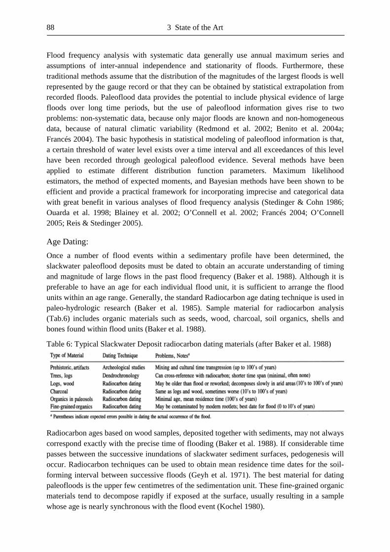
88 3 State of the Art

Flood frequency analysis with systematic data generally use annual maximum series and assumptions of inter-annual independence and stationarity of floods. Furthermore, these traditional methods assume that the distribution of the magnitudes of the largest floods is well represented by the gauge record or that they can be obtained by statistical extrapolation from recorded floods. Paleoflood data provides the potential to include physical evidence of large floods over long time periods, but the use of paleoflood information gives rise to two problems: non-systematic data, because only major floods are known and non-homogeneous data, because of natural climatic variability (Redmond et al. 2002; Benito et al. 2004a; Francés 2004). The basic hypothesis in statistical modeling of paleoflood information is that, a certain threshold of water level exists over a time interval and all exceedances of this level have been recorded through geological paleoflood evidence. Several methods have been applied to estimate different distribution function parameters. Maximum likelihood estimators, the method of expected moments, and Bayesian methods have been shown to be efficient and provide a practical framework for incorporating imprecise and categorical data with great benefit in various analyses of flood frequency analysis (Stedinger & Cohn 1986; Ouarda et al. 1998; Blainey et al. 2002; O’Connell et al. 2002; Francés 2004; O’Connell 2005; Reis & Stedinger 2005). Age Dating:

Once a number of flood events within a sedimentary profile have been determined, the slackwater paleoflood deposits must be dated to obtain an accurate understanding of timing and magnitude of large flows in the past flood frequency (Baker et al. 1988). Although it is preferable to have an age for each individual flood unit, it is sufficient to arrange the flood units within an age range. Generally, the standard Radiocarbon age dating technique is used in paleo-hydrologic research (Baker et al. 1985). Sample material for radiocarbon analysis (Tab.6) includes organic materials such as seeds, wood, charcoal, soil organics, shells and bones found within flood units (Baker et al. 1988). Table 6: Typical Slackwater Deposit radiocarbon dating materials (after Baker et al. 1988)

Radiocarbon ages based on wood samples, deposited together with sediments, may not always correspond exactly with the precise time of flooding (Baker et al. 1988). If considerable time passes between the successive inundations of slackwater sediment surfaces, pedogenesis will occur. Radiocarbon techniques can be used to obtain mean residence time dates for the soil-forming interval between successive floods (Geyh et al. 1971). The best material for dating paleofloods is the upper few centimetres of the sedimentation unit. These fine-grained organic materials tend to decompose rapidly if exposed at the surface, usually resulting in a sample whose age is nearly synchronous with the flood event (Kochel 1980).

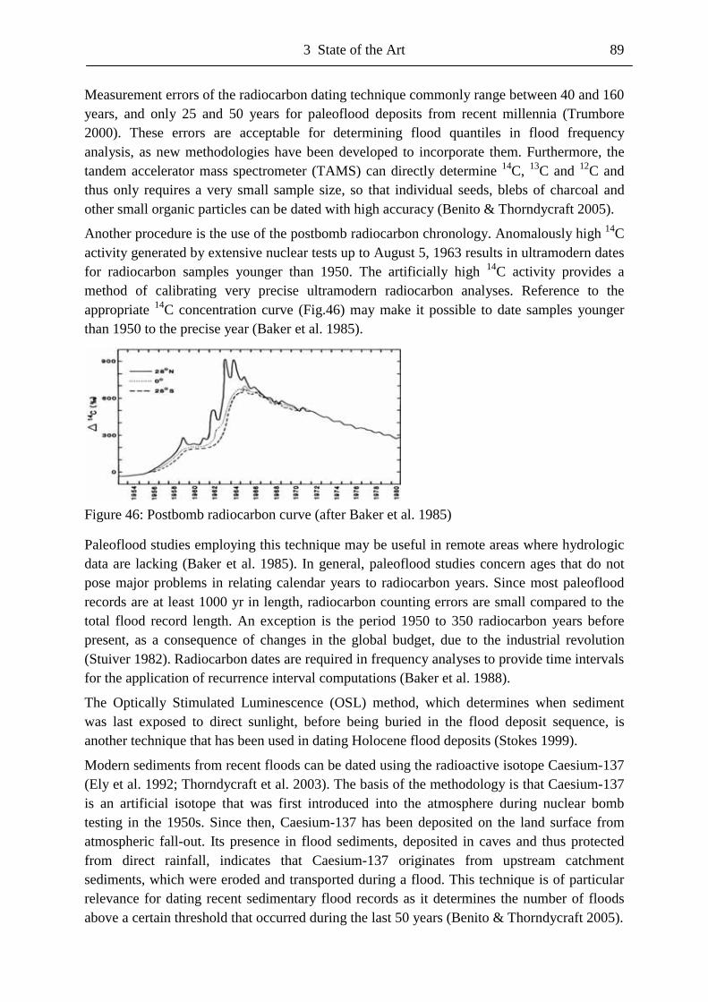
3 State of the Art 89

Measurement errors of the radiocarbon dating technique commonly range between 40 and 160 years, and only 25 and 50 years for paleoflood deposits from recent millennia (Trumbore 2000). These errors are acceptable for determining flood quantiles in flood frequency analysis, as new methodologies have been developed to incorporate them. Furthermore, the tandem accelerator mass spectrometer (TAMS) can directly determine 14C, 13C and 12C and thus only requires a very small sample size, so that individual seeds, blebs of charcoal and other small organic particles can be dated with high accuracy (Benito & Thorndycraft 2005).

Another procedure is the use of the postbomb radiocarbon chronology. Anomalously high 14C activity generated by extensive nuclear tests up to August 5, 1963 results in ultramodern dates for radiocarbon samples younger than 1950. The artificially high 14C activity provides a method of calibrating very precise ultramodern radiocarbon analyses. Reference to the appropriate 14C concentration curve (Fig.46) may make it possible to date samples younger than 1950 to the precise year (Baker et al. 1985).

Figure 46: Postbomb radiocarbon curve (after Baker et al. 1985)

Paleoflood studies employing this technique may be useful in remote areas where hydrologic data are lacking (Baker et al. 1985). In general, paleoflood studies concern ages that do not pose major problems in relating calendar years to radiocarbon years. Since most paleoflood records are at least 1000 yr in length, radiocarbon counting errors are small compared to the total flood record length. An exception is the period 1950 to 350 radiocarbon years before present, as a consequence of changes in the global budget, due to the industrial revolution (Stuiver 1982). Radiocarbon dates are required in frequency analyses to provide time intervals for the application of recurrence interval computations (Baker et al. 1988).

The Optically Stimulated Luminescence (OSL) method, which determines when sediment was last exposed to direct sunlight, before being buried in the flood deposit sequence, is another technique that has been used in dating Holocene flood deposits (Stokes 1999).

Modern sediments from recent floods can be dated using the radioactive isotope Caesium-137 (Ely et al. 1992; Thorndycraft et al. 2003). The basis of the methodology is that Caesium-137 is an artificial isotope that was first introduced into the atmosphere during nuclear bomb testing in the 1950s. Since then, Caesium-137 has been deposited on the land surface from atmospheric fall-out. Its presence in flood sediments, deposited in caves and thus protected from direct rainfall, indicates that Caesium-137 originates from upstream catchment sediments, which were eroded and transported during a flood. This technique is of particular relevance for dating recent sedimentary flood records as it determines the number of floods above a certain threshold that occurred during the last 50 years (Benito & Thorndycraft 2005).

90

4 Methodology 91

4 Methodology 4.1 Isotopes

The stable isotopes oxygen-18 (18O) and deuterium (2H) were measured with a continuous flow isotope ratio mass spectrometer (IRMS) at the University of Freiburg. The pyrolysis of the water samples in a high temperature conversion element analyser is necessary as samples have to be introduced as pure gases. The basic principle of the IRMS is to bend a beam of molecules charged by ionization in a magnetic field into spectrum of masses. Isotopes with higher masses are distracted stronger than isotopes with lower masses. Thus, IRMS allows measuring the relative abundance of isotopes in a given sample. By comparing the detected isotopic ratios to measured lab intern standards an accurate determination of the isotopic content of the sample is obtained. The isotopic concentration values are expressed in relation to a reference, which usually is the Vienna Standard Mean Ocean Water (VSMOV) and are reported in ‰. The relation (�) between the ratios (R) of measured values and reference is given by Clark & Fritz (1997):

1000*���

����

� −=

reference

referencesamplesample R

RRδ [‰] (6)

with OOR 16

18

= or HHR 1

2

= (7)

where �sample = isotopic composition of a sample, R = measured ratio of less and most abundant isotopes. Modern techniques allow the high precise detection of variation in isotope abundance and only small sample volumes are needed (Clark & Fritz 1997). The uncertainty of the IRMS for �2H and �18O is 1 ‰ and 0.2 ‰, respectively.

Stable isotopes show different reaction tendencies of fractionation due to different nuclear masses. These variations of stable isotopes are caused by meteorologic processes. Thus water of a particular environment has a characteristic isotope signature. Fractionation processes modify the ratio of isotopes by transition from one state to another. The higher binding energies of the heavier isotopes explain this phenomenon. More energy is needed to bring heavier isotopes from on energetic level to another. As a consequence heavier isotopes change their nature to a minor degree than lighter isotopes (Gat 1996; Clark & Fritz 1997). According to Dansgaard (1964), there are five fractionation effects, which result in ratio variations of stable isotopes due to fractionation during changes of state.

Continental effect: Decreasing of �18O and �2H values of precipitation with increasing distance from the coast

Altitude effect: Decreasing �18O and �2H values of precipitation with increasing altitude

Latitude effect: Decreasing �18O and �2H values of precipitation with increasing latitude

Amount effect: Decreasing �18O and �2H values of precipitation with increasing amount

Seasonal effect: Increasing amplitude of seasonal variation in the temperature pattern of a site. The greater the seasonal extremes in temperature, the stronger the seasonal variations in �18O and �2H values of precipitation.

92 4 Methodology

4.2 Anions & Cations

The anion concentrations of Cl-, SO42- and NO3

- as well as the cation concentrations of Na+, K+, Mg2+ and Ca2+ have been detected by ion chromatography (IC) at the Institute of Hydrology of the University of Freiburg. Chromatography encompasses numerous physic-chemical separation processes that are based on the distribution of a substance between a mobile and a stationary phase. Ion chromatography allows the separation and detection of ions and polar molecules based on their charge. The uncertainty of IC is about 5 %.

The filtered sample solution is injected into the separating column that consists of an organic polymer, e.g. resin. The used resin is a functional group with a fixed charge. Nearby this functional group, a respective counter-ion from the eluent is located so that the group as a whole is electrically neutral. As a consequence of the different affinity of the anions towards the stationary phase, they become separated. Generally, the retention time of the ion chromatography depends on the length of the separation column, the material within the column, the eluent and the selectivity of the ions. The determination of the ionic composition is done by the detection of conductivity in the suppressor column. The used suppressor SRS ASRS-ULTRA 4 mm reduces the conductivity to a minimum value, while increasing the sample signal/background ratio (Hydrochemical Laboratory 2008, University of Freiburg).

PO43- was analysed according to DEV EN ISO 6878:2004. In this method a calibration line

with the parent solution Merck 1.09879 Titrisol 1000 mg/l PO43- per liter has to be produced.

The dilution steps are 1 ml with 0.02 mg/l to 95 ml with 0.19 mg/l. 4 ml Vogler solution and 1 ml L(+)-Ascorbic acid have to be added to each solution. Then the samples for the calibration line have to be filled up with deionized water up to 100 ml, shaking and for at least 30 minutes they have to be abandoned. To produce the Vogler reagent, 13 g Ammonium heptamolybdate tetrahydrate ((NH4)6Mo7O24 * 4 H2O) have to be solved in 100 ml deionized water and 350 mg Potassium antimony(3)oxide tartarte hydrate (K(SbO)C4H4O6 * 1/2 H2O) in 100 ml as well. First, the molybdate solution and then the tartarte solution are solved by mixing in a 300 ml about 9 molare sulphuric acid solution. The sample volume is 40 ml, but to save sample volume one may work, like I did, with only 10 ml, by diluting the concentrations. The 40 ml are transferred to a 100 ml container. 1 ml 4.5 molar sulphuric acid (H2SO4) is added and mixed. Then 8 ml Potassium peroxodisulfate (K2S2O8) solution is added and mixed. The prepared samples now have to be filled up with deionized water up to 50 ml and have to be abandoned for at least 30 minutes. The samples with high phosphate concentrations become coloured and are measured in a 50 mm cell at 700 nm wave length in a photometer. The analysis of phosphate was undertaken at the Institute of Hydrology of the University of Freiburg with the photometer Aqua Mate.

4 Methodology 93

4.3 Water Samples

Streamflow samples were taken for two complete months in October 2008 and November 2009. In October 2008, 118 water samples were taken during and after the extreme flood and analyzed for the nutrients Na+, K+, Mg2+, Ca2+, Cl-, SO4

2-, NO3- and PO4

3- as well as for the isotopes �18O and �2H. For the 83 water samples taken in the dry period of November 2009 conductivity, pH and sediment concentrations are available yet. Nutrients and isotopes need to be determined to complete the picture of water chemistry for these two extreme climatic situations. The first month marks the change from rainy season to the drier month of the year and starts with a sample taken on 11.10, 12 a.m., 4 hours before the rainstorm. The sample period for the first month is from 11.10, 12 a.m. to 12.11, 12 p.m. For a better visualization and separation of the ongoing processes the study month was divided into three phases. The first phase, the flood phase represents the pure influence of the rainstorm of 11th October 2008 and lasts for nearly two days from 11.10, 12 a.m. to 13.10, 10 a.m. The second phase, the recovery phase, represents the long-term impact of the rainstorm on the composition of streamflow and lasts for about eight days from 13.10, 2 p.m. to 21.10, 6 a.m. The third phase, the post-flood phase is characterized by three normal water floods. The first two post-flood events are characterized by a fast stream response and relatively high sediment concentrations. The post-flood phase lasts from 21.10, 12 a.m. to 12.11, 12 p.m.

The first taken sample is included in the hydrochemical diagrams to better visualize the sudden rise of discharge and according change in chemical composition, but not in the Box Plots and in the presented calculations. Thus the chemical hydrographs assume that stream composition did not change in the five hours before peak discharge. Accordingly, the first two samples at 12 a.m. and 5 p.m. on 11.10 both represent the sample taken at 12 a.m. It has to be noted that something went wrong in the analysis of this sample, showing unrealistic high contents of chloride and potassium. Probably pH was measured within the sample bottle. Therefore, both nutrients were excluded from analysis and the respective nutrient concentrations are not depicted in the chemographs so that chloride and potassium concentrations start with the three samples taken at 5.18, 5.20, 5.21 p.m. on 11.10. Because these three samples only represent five minutes of the mudflow phase, they are treated as one sample, given their average concentration. Due to a misunderstanding there is a gap of two hours in sample taking from these three samples until 7.15 p.m. so that the water chemistry in the first 2.25 hours after peak discharge is unknown. As the rainstorm lasted about 1.5 hours from 4 p.m. to 5.30 p.m. and took mainly place in the headwaters near the watersheds, most notably at the ‘El Tiro’ watershed, rainfall intensities in all diagrams were used for the ‘El Tiro’ meteorologic station. The climatic data for the dry period 2009 derive from the ECSF meteorologic station. The samples of the dry period 2009 range from 05.11, 12 a.m. to 05.12, 12 a.m.

94 4 Methodology

4.4 Sediment

When sampling streams for suspended sediment it is important to obtain samples that reflect the actual sediment loads of the stream. Samples must be taken in such a way that the concentration represents an average for the cross-section, because the sediment concentration distribution varies with depth and across the section largely depending on particle size. When the natural mixing effect of turbulence is exploited the taken sample is considered to be relatively homogeneous (Gordon et al. 2004). All water samples were taken at the same location and used the natural turbulence of the stream.

A method to measure the sediment concentration of a taken suspension of known volume is to evaporate all the contained water. The dried sediments then can be weighted. To save drying time, sediment-free water can be siphoned or poured off, when the sediment sample has settled for at least 12 h. Sediment concentration (cS) is calculated by:

[ ]lgcS /suspension of volume

sediment= (8)

where sediment is in g and suspension volume is in l. The evaporation method measures both sediment concentration and dissolved solids. Thus, the technique is best for streams where the salt-mineral content is low in comparison with the suspended load, like in headwater streams or during high sediment transport (Gordon et al. 2004). 4.5 Cross-sectional Measurements

Cross-sectional measurements were done by stretching a tape across the river and fix it in the height of the flood marks. High water marks were present on both river sides for all measured cross-sections. The perpendicular was taken every meter. Additionally the water surface inclination or super-elevation was determined with an inclinometer. The inclinometer was also used to determine the hillslope angles and the bed slope. To obtain precise values of the bed slope, long distances of about 50 – 100 m have been measured, except in bends where the measuring length was about 20 - 50 m. Of the 40 measured cross-sections, 15 were selected to calculate discharge with the slope-area method, by using both Manning’s and Chezy’s equation. The same cross-sections were used in the one-dimensional hydraulic model HEC-RAS 4.0 to validate the obtained parameters from the slope-area method.

The most important factor in selecting suitable reaches for paleoflood analysis is the existence of multiple paleostage indicators. Channel boundaries should be both, horizontally and vertically stable. Hydraulically simple reaches can be more accurately modeled than complex reaches. The number of transitions between subcritical-supercritical flow regimes and their associated unaccountable energy losses should be kept as low as possible and the modeled reach should be long enough to account for uncertainties in the elevation of high-water indicators (Dalrymple & Benson 1967). Beside the reach geometry, the positions and elevations of paleostage indicators and estimates of Manning’s n values are required. The most precise matching of step-backwater generated water surface profiles to profiles defined by paleostage indicators can be achieved by adjacent cross-sections that contain paleostage indicators (Baker et al. 1988).

4 Methodology 95

4.6 Slope-area Method

At first, some definitions: Depth = D; vertical distance (m) between the water surface and some point on the streambed; Stage = y; vertical distance (m) from some fixed datum to the water surface. The datum might be the elevation of zero flow or mean sea level; Discharge = Q; volume of water (m3/s) passing through a stream cross-section per unit time; Top width = W; width (m) of the stream at the water surface. Except in channels with vertical walls, it will vary with stream depth. Cross-sectional area = A; area (m2) of water across a given section of the stream. Wetted perimeter = P; distance (m) around the outside edge of the cross-sectional ‘slice’ where the stream’s bed and banks contact the water; Hydraulic radius = R; ratio (m) of the cross-sectional area to the wetted perimeter: R = A/P; Hydraulic depth = D; ratio (m) of the cross-sectional area to the top width: D = A/W (Baker et al. 1988).

The basic idea in open channel flow is to determine the relationship between stage and discharge by correlating measurements of discharge with observations of stage. In a stable channel that is defined as one in which the physical form, control characteristics and frictional properties of the river channel remain constant with respect to time, the stage-discharge relationship is expressed in the basic formulae (Gordon et al. 2004):

nhhCQ )( 0+= (9)

where Q = discharge (m3/s), h = stage (m), h0 = zero correction (m), C, n = parameters to be determined by observation. The correction factor h0 needs to be determined, if the zero of the gauge does not coincide with zero discharge (Herschy 1978).

At ungauged sites, peak discharges during flood events are often indirectly estimated from the height of water marks left behind. Indirect methods can also be used to extend the upper part of a stage-discharge relationship (Herschy 1985). The slope-area method is a commonly used technique for indirect estimation of discharge (Dalrymple & Benson 1967). The stage-discharge relationship for simple prismatic channels can be obtained by applying a uniform flow resistance formula such as the most spread Manning’s or Chezy’s equation:

Manning 21

32

***1fh SRA

nQ = (10)

Chezy 21

21

*** fh SRACQ = (11)

Chezy coefficient fh SR

vC∗

= (12)

where Q = discharge (m3/s), A = area of cross-section (m2), Rh = hydraulic radius (m), whereas Rh =A/P, P = wetted perimeter (m), Sf = energy slope, whereas under uniform flow conditions Sf = S0 (bed slope), C = Chezy’s resistance coefficient and n = Manning’s roughness coefficient. The hydraulic parameters A, P and R in the equations (10) and (11) are related to the depth of flow h and depend on the shape of the cross-sectional profile. For the method to be valid a reach must be carefully selected so that uniform flow conditions can be approximated. This means that channel width, depth of flow, flow velocity, streambed materials and channel slope remain constant over a straight reach, as well as that channel

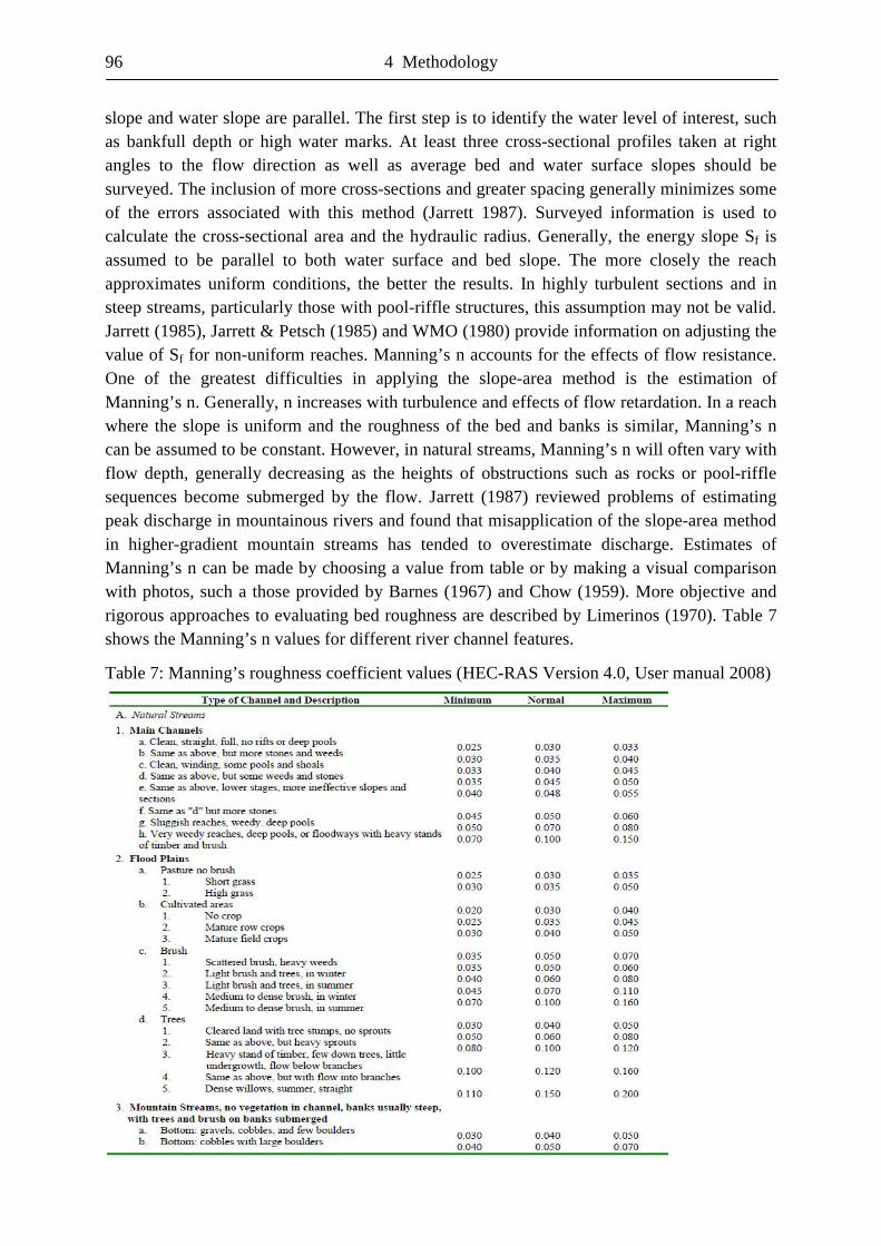
96 4 Methodology

slope and water slope are parallel. The first step is to identify the water level of interest, such as bankfull depth or high water marks. At least three cross-sectional profiles taken at right angles to the flow direction as well as average bed and water surface slopes should be surveyed. The inclusion of more cross-sections and greater spacing generally minimizes some of the errors associated with this method (Jarrett 1987). Surveyed information is used to calculate the cross-sectional area and the hydraulic radius. Generally, the energy slope Sf is assumed to be parallel to both water surface and bed slope. The more closely the reach approximates uniform conditions, the better the results. In highly turbulent sections and in steep streams, particularly those with pool-riffle structures, this assumption may not be valid. Jarrett (1985), Jarrett & Petsch (1985) and WMO (1980) provide information on adjusting the value of Sf for non-uniform reaches. Manning’s n accounts for the effects of flow resistance. One of the greatest difficulties in applying the slope-area method is the estimation of Manning’s n. Generally, n increases with turbulence and effects of flow retardation. In a reach where the slope is uniform and the roughness of the bed and banks is similar, Manning’s n can be assumed to be constant. However, in natural streams, Manning’s n will often vary with flow depth, generally decreasing as the heights of obstructions such as rocks or pool-riffle sequences become submerged by the flow. Jarrett (1987) reviewed problems of estimating peak discharge in mountainous rivers and found that misapplication of the slope-area method in higher-gradient mountain streams has tended to overestimate discharge. Estimates of Manning’s n can be made by choosing a value from table or by making a visual comparison with photos, such a those provided by Barnes (1967) and Chow (1959). More objective and rigorous approaches to evaluating bed roughness are described by Limerinos (1970). Table 7 shows the Manning’s n values for different river channel features. Table 7: Manning’s roughness coefficient values (HEC-RAS Version 4.0, User manual 2008)

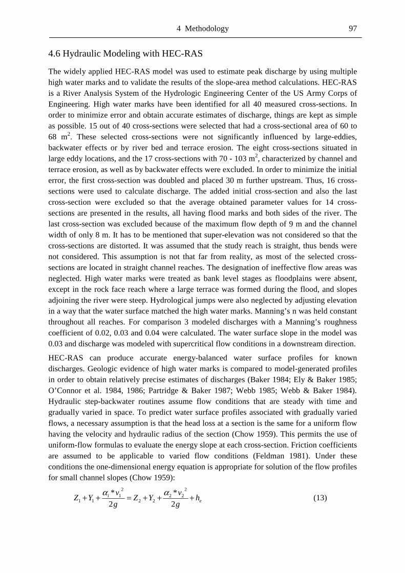
4 Methodology 97

4.6 Hydraulic Modeling with HEC-RAS

The widely applied HEC-RAS model was used to estimate peak discharge by using multiple high water marks and to validate the results of the slope-area method calculations. HEC-RAS is a River Analysis System of the Hydrologic Engineering Center of the US Army Corps of Engineering. High water marks have been identified for all 40 measured cross-sections. In order to minimize error and obtain accurate estimates of discharge, things are kept as simple as possible. 15 out of 40 cross-sections were selected that had a cross-sectional area of 60 to 68 m2. These selected cross-sections were not significantly influenced by large-eddies, backwater effects or by river bed and terrace erosion. The eight cross-sections situated in large eddy locations, and the 17 cross-sections with 70 - 103 m2, characterized by channel and terrace erosion, as well as by backwater effects were excluded. In order to minimize the initial error, the first cross-section was doubled and placed 30 m further upstream. Thus, 16 cross-sections were used to calculate discharge. The added initial cross-section and also the last cross-section were excluded so that the average obtained parameter values for 14 cross-sections are presented in the results, all having flood marks and both sides of the river. The last cross-section was excluded because of the maximum flow depth of 9 m and the channel width of only 8 m. It has to be mentioned that super-elevation was not considered so that the cross-sections are distorted. It was assumed that the study reach is straight, thus bends were not considered. This assumption is not that far from reality, as most of the selected cross-sections are located in straight channel reaches. The designation of ineffective flow areas was neglected. High water marks were treated as bank level stages as floodplains were absent, except in the rock face reach where a large terrace was formed during the flood, and slopes adjoining the river were steep. Hydrological jumps were also neglected by adjusting elevation in a way that the water surface matched the high water marks. Manning’s n was held constant throughout all reaches. For comparison 3 modeled discharges with a Manning’s roughness coefficient of 0.02, 0.03 and 0.04 were calculated. The water surface slope in the model was 0.03 and discharge was modeled with supercritical flow conditions in a downstream direction.

HEC-RAS can produce accurate energy-balanced water surface profiles for known discharges. Geologic evidence of high water marks is compared to model-generated profiles in order to obtain relatively precise estimates of discharges (Baker 1984; Ely & Baker 1985; O’Connor et al. 1984, 1986; Partridge & Baker 1987; Webb 1985; Webb & Baker 1984). Hydraulic step-backwater routines assume flow conditions that are steady with time and gradually varied in space. To predict water surface profiles associated with gradually varied flows, a necessary assumption is that the head loss at a section is the same for a uniform flow having the velocity and hydraulic radius of the section (Chow 1959). This permits the use of uniform-flow formulas to evaluate the energy slope at each cross-section. Friction coefficients are assumed to be applicable to varied flow conditions (Feldman 1981). Under these conditions the one-dimensional energy equation is appropriate for solution of the flow profiles for small channel slopes (Chow 1959):

ei h

gvYZ

gvYZ +++=++

2*

2* 2

2222

21

11αα (13)

98 4 Methodology

where z = elevation of the channel above an arbitrary datum (m), y = flow depth (m), v = mean flow velocity (m/s), g = gravitational acceleration (9.81 m/s2), = velocity head (m) coefficient accounting for non-uniform velocity distribution in a subdivided channel, he = head loss (m) between cross-sections. Figure 47 defines this formula (Baker et al. 1988):

Figure 47: Conservation of energy for gradually varied flow (Baker et al. 1988)

In natural stream systems, the water surface slope may deviate locally from both the channel slope and the energy slope depending on the local channel geometry (Baker et al. 1988). Equation (13) expresses conservation of mechanical energy for gradually varied flow within an incremental reach of channel. The sum of a flow’s potential and kinetic energy must equal that of a downstream cross-section less any energy losses between sections. Head loss is subdivided into frictional losses created by flow boundary roughness elements, eddy losses associated with turbulence, and flow separation generated by channel constrictions and expansions. Friction losses are evaluated by a variation of the Manning equation:

3/4

22 *R

vnS f = (14)

where Sf = local friction slope, n = Manning’s roughness coefficient, v = flow velocity (m/s) and R = hydraulic radius (m). Eddy losses are calculated as a function of the change in velocity head between sections:

gv

gvkEddyloss

22

222

211 αα −= (15)

where k is taken to equal 0 - 0.1 for gradually narrowing reaches: 1v12/2g < 2v2

2/2g and 0.2 - 0.5 for expanding reaches: 1v1

2/2g < 2v22/2g (Chow 1959; Dalrymple & Benson 1967;

Hydrologic Engineering Center 1982).

Some step-backwater routines do not have the capability to evaluate eddy losses directly; therefore, this type of energy loss must also be accounted for in selection of local Manning’s n coefficients. The use of the Manning equation local friction slopes allows a solution to Equation (1) given initial stage, discharge conditions, and known channel geometry. The computational approach, the “standard step” method described by Chow (1959), is an iterative procedure where successive attempts are made at determining an energy-balanced water surface elevation. The final estimated water surface elevation at the unknown section must have an associated energy that equals the total energy of the cross-section of known flow conditions, less any calculated head losses between them. The newly predicted water surface

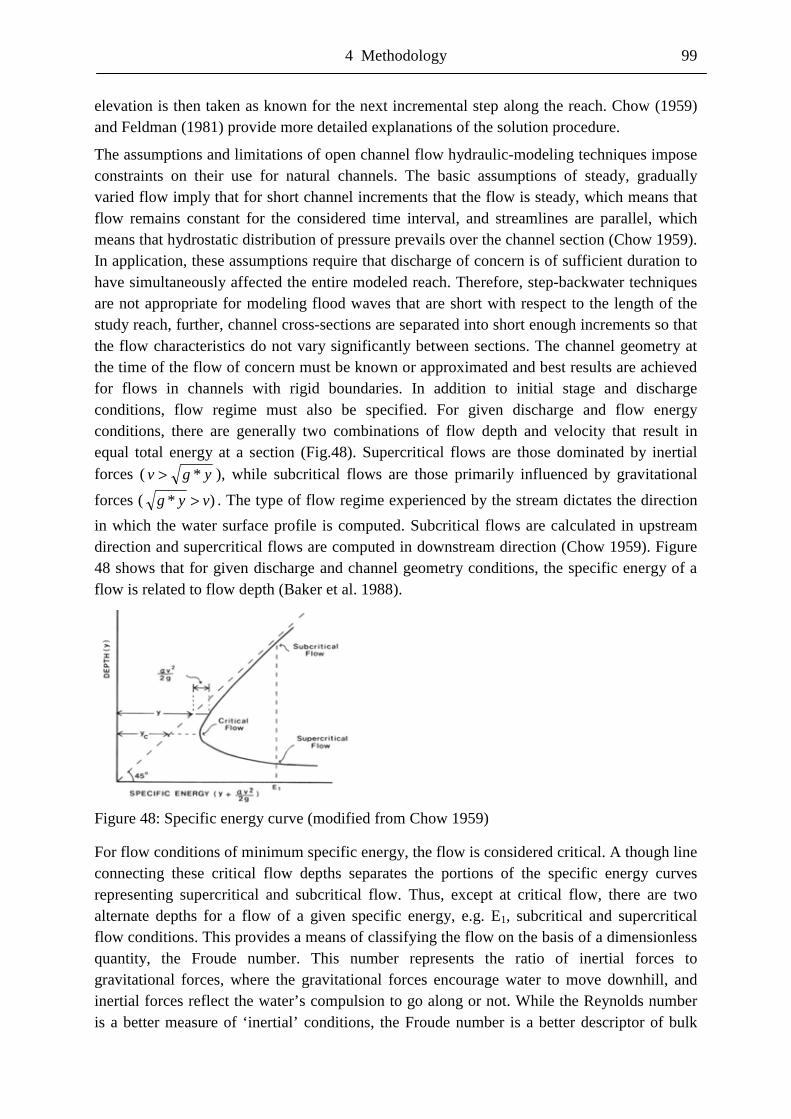
4 Methodology 99

elevation is then taken as known for the next incremental step along the reach. Chow (1959) and Feldman (1981) provide more detailed explanations of the solution procedure.

The assumptions and limitations of open channel flow hydraulic-modeling techniques impose constraints on their use for natural channels. The basic assumptions of steady, gradually varied flow imply that for short channel increments that the flow is steady, which means that flow remains constant for the considered time interval, and streamlines are parallel, which means that hydrostatic distribution of pressure prevails over the channel section (Chow 1959). In application, these assumptions require that discharge of concern is of sufficient duration to have simultaneously affected the entire modeled reach. Therefore, step-backwater techniques are not appropriate for modeling flood waves that are short with respect to the length of the study reach, further, channel cross-sections are separated into short enough increments so that the flow characteristics do not vary significantly between sections. The channel geometry at the time of the flow of concern must be known or approximated and best results are achieved for flows in channels with rigid boundaries. In addition to initial stage and discharge conditions, flow regime must also be specified. For given discharge and flow energy conditions, there are generally two combinations of flow depth and velocity that result in equal total energy at a section (Fig.48). Supercritical flows are those dominated by inertial forces ( ygv *> ), while subcritical flows are those primarily influenced by gravitational forces ( )* vyg > . The type of flow regime experienced by the stream dictates the direction in which the water surface profile is computed. Subcritical flows are calculated in upstream direction and supercritical flows are computed in downstream direction (Chow 1959). Figure 48 shows that for given discharge and channel geometry conditions, the specific energy of a flow is related to flow depth (Baker et al. 1988).

Figure 48: Specific energy curve (modified from Chow 1959)

For flow conditions of minimum specific energy, the flow is considered critical. A though line connecting these critical flow depths separates the portions of the specific energy curves representing supercritical and subcritical flow. Thus, except at critical flow, there are two alternate depths for a flow of a given specific energy, e.g. E1, subcritical and supercritical flow conditions. This provides a means of classifying the flow on the basis of a dimensionless quantity, the Froude number. This number represents the ratio of inertial forces to gravitational forces, where the gravitational forces encourage water to move downhill, and inertial forces reflect the water’s compulsion to go along or not. While the Reynolds number is a better measure of ‘inertial’ conditions, the Froude number is a better descriptor of bulk

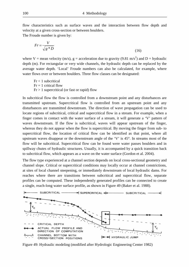
100 4 Methodology

flow characteristics such as surface waves and the interaction between flow depth and velocity at a given cross-section or between boulders. The Froude number is given by:

Dg

VFr*

= (16)

where V = mean velocity (m/s), g = acceleration due to gravity (9.81 m/s2) and D = hydraulic depth (m). For rectangular or very wide channels, the hydraulic depth can be replaced by the average water depth. ‘Local’ Froude numbers can also be calculated, for example, where water flows over or between boulders. Three flow classes can be designated: Fr < 1 subcritical Fr = 1 critical flow Fr > 1 supercritical (or fast or rapid) flow

In subcritical flow the flow is controlled from a downstream point and any disturbances are transmitted upstream. Supercritical flow is controlled from an upstream point and any disturbances are transmitted downstream. The direction of wave propagation can be used to locate regions of subcritical, critical and supercritical flow in a stream. For example, when a finger comes in contact with the water surface of a stream, it will generate a ‘V’ pattern of waves downstream. If the flow is subcritical, waves will appear upstream of the finger, whereas they do not appear when the flow is supercritical. By moving the finger from sub- to supercritical flow, the location of critical flow can be identified as that point, where all upstream waves disappear or the downstream angle of the ‘V’ is 45°. In streams most of the flow will be subcritical. Supercritical flow can be found were water passes boulders and in spillway chutes of hydraulic structures. Usually, it is accompanied by a quick transition back to subcritical flow, which appears as a wave on the water surface (Gordon et al. 2004).

The flow type experienced at a channel section depends on local cross-sectional geometry and channel slope. Critical or supercritical conditions may locally occur at channel constrictions, at sites of local channel steepening, or immediately downstream of local hydraulic dams. For reaches where there are transitions between subcritical and supercritical flow, separate profiles can be computed. These independently generated profiles can be connected to create a single, reach-long water surface profile, as shown in Figure 49 (Baker et al. 1988).

Figure 49: Hydraulic modeling (modified after Hydrologic Engineering Center 1982)

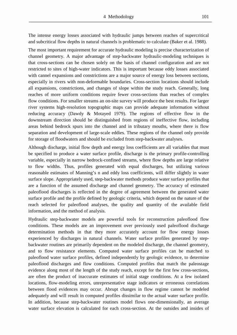
4 Methodology 101

The intense energy losses associated with hydraulic jumps between reaches of supercritical and subcritical flow depths in natural channels is problematic to calculate (Baker et al. 1988).

The most important requirement for accurate hydraulic modeling is precise characterization of channel geometry. A major advantage of step-backwater hydraulic-modeling techniques is that cross-sections can be chosen solely on the basis of channel configuration and are not restricted to sites of high-water indicators. This is important because eddy losses associated with cannel expansions and constrictions are a major source of energy loss between sections, especially in rivers with non-deformable boundaries. Cross-section locations should include all expansions, constrictions, and changes of slope within the study reach. Generally, long reaches of more uniform conditions require fewer cross-sections than reaches of complex flow conditions. For smaller streams an on-site survey will produce the best results. For larger river systems high-resolution topographic maps can provide adequate information without reducing accuracy (Dawdy & Motayed 1979). The regions of effective flow in the downstream direction should be distinguished from regions of ineffective flow, including areas behind bedrock spurs into the channel and in tributary mouths, where there is flow separation and development of large-scale eddies. These regions of the channel only provide for storage of floodwaters and should be excluded from step-backwater analyses.

Although discharge, initial flow depth and energy loss coefficients are all variables that must be specified to produce a water surface profile, discharge is the primary profile-controlling variable, especially in narrow bedrock-confined streams, where flow depths are large relative to flow widths. Thus, profiles generated with equal discharges, but utilizing various reasonable estimates of Manning’s n and eddy loss coefficients, will differ slightly in water surface slope. Appropriately used, step-backwater methods produce water surface profiles that are a function of the assumed discharge and channel geometry. The accuracy of estimated paleoflood discharges is reflected in the degree of agreement between the generated water surface profile and the profile defined by geologic criteria, which depend on the nature of the reach selected for paleoflood analyses, the quality and quantity of the available field information, and the method of analysis.

Hydraulic step-backwater models are powerful tools for reconstruction paleoflood flow conditions. These models are an improvement over previously used paleoflood discharge determination methods in that they more accurately account for flow energy losses experienced by discharges in natural channels. Water surface profiles generated by step-backwater routines are primarily dependent on the modeled discharge, the channel geometry, and to flow resistance elements. Computed water surface profiles can be matched to paleoflood water surface profiles, defined independently by geologic evidence, to determine paleoflood discharges and flow conditions. Computed profiles that match the paleostage evidence along most of the length of the study reach, except for the first few cross-sections, are often the product of inaccurate estimates of initial stage conditions. At a few isolated locations, flow-modeling errors, unrepresentative stage indicators or erroneous correlations between flood evidences may occur. Abrupt changes in flow regime cannot be modeled adequately and will result in computed profiles dissimilar to the actual water surface profile. In addition, because step-backwater routines model flows one-dimensionally, an average water surface elevation is calculated for each cross-section. At the outsides and insides of

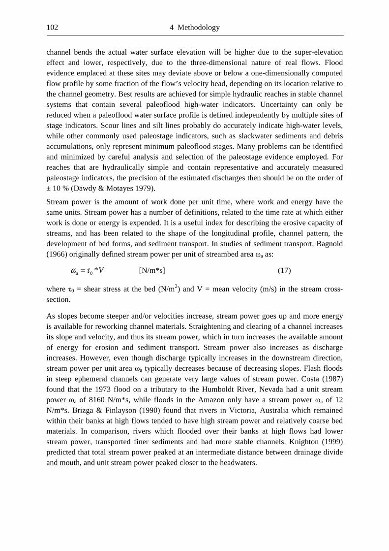
102 4 Methodology

channel bends the actual water surface elevation will be higher due to the super-elevation effect and lower, respectively, due to the three-dimensional nature of real flows. Flood evidence emplaced at these sites may deviate above or below a one-dimensionally computed flow profile by some fraction of the flow’s velocity head, depending on its location relative to the channel geometry. Best results are achieved for simple hydraulic reaches in stable channel systems that contain several paleoflood high-water indicators. Uncertainty can only be reduced when a paleoflood water surface profile is defined independently by multiple sites of stage indicators. Scour lines and silt lines probably do accurately indicate high-water levels, while other commonly used paleostage indicators, such as slackwater sediments and debris accumulations, only represent minimum paleoflood stages. Many problems can be identified and minimized by careful analysis and selection of the paleostage evidence employed. For reaches that are hydraulically simple and contain representative and accurately measured paleostage indicators, the precision of the estimated discharges then should be on the order of ± 10 % (Dawdy & Motayes 1979).

Stream power is the amount of work done per unit time, where work and energy have the same units. Stream power has a number of definitions, related to the time rate at which either work is done or energy is expended. It is a useful index for describing the erosive capacity of streams, and has been related to the shape of the longitudinal profile, channel pattern, the development of bed forms, and sediment transport. In studies of sediment transport, Bagnold (1966) originally defined stream power per unit of streambed area �a as:

Va *0τω = [N/m*s] (17)

where �0 = shear stress at the bed (N/m2) and V = mean velocity (m/s) in the stream cross-section.

As slopes become steeper and/or velocities increase, stream power goes up and more energy is available for reworking channel materials. Straightening and clearing of a channel increases its slope and velocity, and thus its stream power, which in turn increases the available amount of energy for erosion and sediment transport. Stream power also increases as discharge increases. However, even though discharge typically increases in the downstream direction, stream power per unit area �a typically decreases because of decreasing slopes. Flash floods in steep ephemeral channels can generate very large values of stream power. Costa (1987) found that the 1973 flood on a tributary to the Humboldt River, Nevada had a unit stream power �a of 8160 N/m*s, while floods in the Amazon only have a stream power �a of 12 N/m*s. Brizga & Finlayson (1990) found that rivers in Victoria, Australia which remained within their banks at high flows tended to have high stream power and relatively coarse bed materials. In comparison, rivers which flooded over their banks at high flows had lower stream power, transported finer sediments and had more stable channels. Knighton (1999) predicted that total stream power peaked at an intermediate distance between drainage divide and mouth, and unit stream power peaked closer to the headwaters.

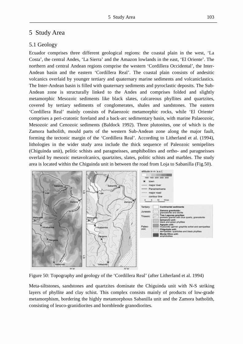
5 Study Area 103

5 Study Area

5.1 Geology Ecuador comprises three different geological regions: the coastal plain in the west, ‘La Costa’, the central Andes, ‘La Sierra’ and the Amazon lowlands in the east, ‘El Oriente’. The northern and central Andean regions comprise the western ‘Cordillera Occidental’, the Inter-Andean basin and the eastern ‘Cordillera Real’. The coastal plain consists of andesitic volcanics overlaid by younger tertiary and quaternary marine sediments and volcaniclastics. The Inter-Andean basin is filled with quaternary sediments and pyroclastic deposits. The Sub-Andean zone is structurally linked to the Andes and comprises folded and slightly metamorphic Mesozoic sediments like black slates, calcareous phyllites and quartzites, covered by tertiary sediments of conglomerates, shales and sandstones. The eastern ‘Cordillera Real’ mainly consists of Palaeozoic metamorphic rocks, while ‘El Oriente’ comprises a peri-cratonic foreland and a back-arc sedimentary basin, with marine Palaeozoic, Mesozoic and Cenozoic sediments (Baldock 1992). Three plutonites, one of which is the Zamora batholith, mould parts of the western Sub-Andean zone along the major fault, forming the tectonic margin of the ‘Cordillera Real’. According to Litherland et al. (1994), lithologies in the wider study area include the thick sequence of Paleozoic semipelites (Chiguinda unit), pelitic schists and paragneisses, amphibolites and ortho- and paragneisses overlaid by mesozic metavolcanics, quartzites, slates, politic schists and marbles. The study area is located within the Chiguinda unit in between the road from Loja to Sabanilla (Fig.50).

Figure 50: Topography and geology of the ‘Cordillera Real’ (after Litherland et al. 1994)

Meta-siltstones, sandstones and quartzites dominate the Chiguinda unit with N-S striking layers of phyllite and clay schist. This complex consists mainly of products of low-grade metamorphism, bordering the highly metamorphous Sabanilla unit and the Zamora batholith, consisting of leuco-granidiorites and hornblende granodiorites.

104 5 Study Area

The famous Ecuadorian mountains, such as the volcanoes Chimborazo, Cotopaxi or Antisana, with altitudes around 6000 m are concentrated in north and central Ecuador. In contrast, volcanoes in the Andean depression in south Ecuador (Fig.51) are absent and the crest of the ‘Cordillera Real’ does not exceed 2750 - 3400 m (Beck et al. 2008).

Figure 51: Position of the upper tree line and lowest glacial stands within the Neotropical section of the western escarpment of the Andes (Richter et al. 2008)

The lowest regions in the ‘Cordillera Real’ are the breach of the Rio Zamora, crossing the eastern mountain range of the Andes north of Loja and the ‘El Tiro’ watershed east of Loja with an altitude of 2000 m and 2750 m, respectively (Fig.52).

Figure 52: Study area below the ‘El Tiro’ watershed, ‘Cordillera Real’ (Google Earth 2010)

Even in such low positions, features of Pleistocene glaciation are present, such as head walls behind cirques containing tarns, e.g. ‘Lagunas de los Compadres’ south of the study area, smoothened bedrock with truncated spurs, and lateral and terminal moraines forming a typical nunatak landscape.

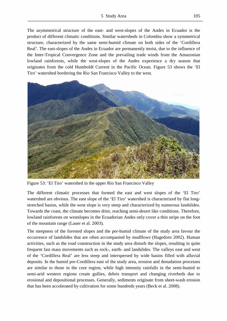
5 Study Area 105

The asymmetrical structure of the east- and west-slopes of the Andes in Ecuador is the product of different climatic conditions. Similar watersheds in Colombia show a symmetrical structure, characterized by the same semi-humid climate on both sides of the ‘Cordillera Real’. The east-slopes of the Andes in Ecuador are permanently moist, due to the influence of the Inter-Tropical Convergence Zone and the prevailing trade winds from the Amazonian lowland rainforests, while the west-slopes of the Andes experience a dry season that originates from the cold Humboldt Current in the Pacific Ocean. Figure 53 shows the ‘El Tiro’ watershed bordering the Rio San Francisco Valley to the west.

Figure 53: ‘El Tiro’ watershed in the upper Rio San Francisco Valley

The different climatic processes that formed the east and west slopes of the ‘El Tiro’ watershed are obvious. The east slope of the ‘El Tiro’ watershed is characterized by flat long-stretched basins, while the west slope is very steep and characterized by numerous landslides. Towards the coast, the climate becomes drier, reaching semi-desert like conditions. Therefore, lowland rainforests on westslopes in the Ecuadorian Andes only cover a thin stripe on the foot of the mountain range (Lauer et al. 2003).

The steepness of the forested slopes and the per-humid climate of the study area favour the occurrence of landslides that are often accompanied by mudflows (Hagedorn 2002). Human activities, such as the road construction in the study area disturb the slopes, resulting in quite frequent fast mass movements such as rock-, earth- and landslides. The valleys east and west of the ‘Cordillera Real’ are less steep and interspersed by wide basins filled with alluvial deposits. In the humid pre-Cordillera east of the study area, erosion and denudation processes are similar to those in the core region, while high intensity rainfalls in the semi-humid to semi-arid western regions create gullies, debris transport and changing riverbeds due to erosional and depositional processes. Generally, sediments originate from sheet-wash erosion that has been accelerated by cultivation for some hundreds years (Beck et al. 2008).

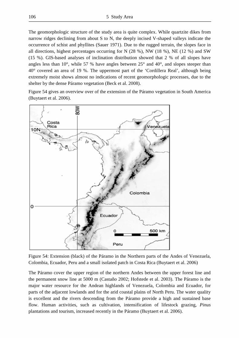
106 5 Study Area

The geomorphologic structure of the study area is quite complex. While quartzite dikes from narrow ridges declining from about S to N, the deeply incised V-shaped valleys indicate the occurrence of schist and phyllites (Sauer 1971). Due to the rugged terrain, the slopes face in all directions, highest percentages occurring for N (28 %), NW (18 %), NE (12 %) and SW (15 %). GIS-based analyses of inclination distribution showed that 2 % of all slopes have angles less than 10°, while 57 % have angles between 25° and 40°, and slopes steeper than 40° covered an area of 19 %. The uppermost part of the ‘Cordillera Real’, although being extremely moist shows almost no indications of recent geomorphologic processes, due to the shelter by the dense Páramo vegetation (Beck et al. 2008).

Figure 54 gives an overview over of the extension of the Páramo vegetation in South America (Buytaert et al. 2006).

Figure 54: Extension (black) of the Páramo in the Northern parts of the Andes of Venezuela, Colombia, Ecuador, Peru and a small isolated patch in Costa Rica (Buytaert et al. 2006)

The Páramo cover the upper region of the northern Andes between the upper forest line and the permanent snow line at 5000 m (Castaño 2002; Hofstede et al. 2003). The Páramo is the major water resource for the Andean highlands of Venezuela, Colombia and Ecuador, for parts of the adjacent lowlands and for the arid coastal plains of North Peru. The water quality is excellent and the rivers descending from the Páramo provide a high and sustained base flow. Human activities, such as cultivation, intensification of lifestock grazing, Pinus plantations and tourism, increased recently in the Páramo (Buytaert et al. 2006).

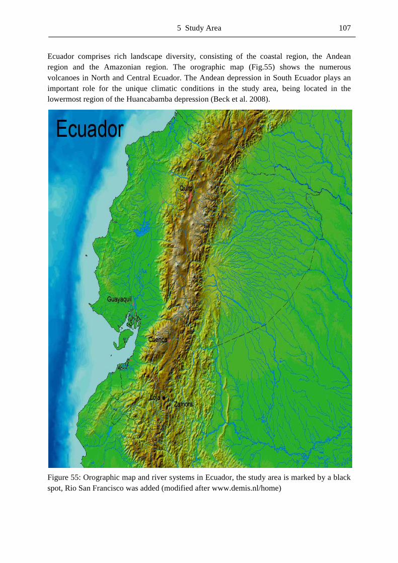
5 Study Area 107

Ecuador comprises rich landscape diversity, consisting of the coastal region, the Andean region and the Amazonian region. The orographic map (Fig.55) shows the numerous volcanoes in North and Central Ecuador. The Andean depression in South Ecuador plays an important role for the unique climatic conditions in the study area, being located in the lowermost region of the Huancabamba depression (Beck et al. 2008).

Figure 55: Orographic map and river systems in Ecuador, the study area is marked by a black spot, Rio San Francisco was added (modified after www.demis.nl/home)

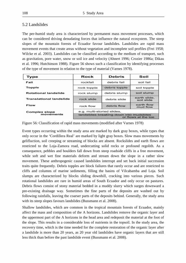
108 5 Study Area

5.2 Landslides

The per-humid study area is characterized by permanent mass movement processes, which can be considered driving denudating forces that influence the natural ecosystem. The steep slopes of the mountain forests of Ecuador favour landslides. Landslides are rapid mass movement events that create areas without vegetation and incomplete soil profiles (Frei 1958; Wilcke et al. 2003). Landslides can be classified according to the medium of transport, such as gravitation, pore water, snow or soil ice and velocity (Ahnert 1996; Crozier 1986a; Dikau et al. 1996; Hutchinson 1988). Figure 56 shows such a classification by identifying processes of the type of movement in relation to the type of material (Varnes 1978).

Figure 56: Classification of rapid mass movements (modified after Varnes 1978)

Event types occurring within the study area are marked by dark gray boxes, while types that only occur in the ‘Cordillera Real’ are marked by light gray boxes. Slow mass movements by gelifluction, soil creeping or streaming of blocks are absent. Rockslides and earth flows are restricted to the Loja-Zamora road, undercutting solid rocks or profound regolith. As a consequence, pebbles and boulders fall down from steep roadside cliffs in a free movement, while soft and wet fine materials deform and stream down the slope in a rather slow movement. These anthropogenic caused landslides interrupt and set back initial succession traits quite frequently. Debris topples are block failures that rarely occur and are restricted to cliffs and columns of marine sediments, filling the basins of Vilcabamba and Loja. Soil slumps are characterized by blocks sliding downhill, cracking into various pieces. Such rotational landslides are rare in humid areas of South Ecuador and only occur on pastures. Debris flows consist of stony material bedded in a muddy slurry which surges downward a pre-existing drainage way. Sometimes the fine parts of the deposits are washed out by following rainfalls, leaving the coarser parts of the deposits behind. Generally, the study area with its steep slopes favours landslides (Bussmann et al. 2008).

Shallow landslides, which are common in the tropical mountain forests of Ecuador, mainly affect the mass and composition of the A horizons. Landslides remove the organic layer and the uppermost part of the A horizons in the head area and redeposit the material at the foot of the slope. This results in a considerable loss of nutrients in the topsoil. In the study area, the recovery time, which is the time needed for the complete restoration of the organic layer after a landslide is more than 20 years, as 20 year old landslides have organic layers that are still less thick than before the past landslide event (Bussmann et al. 2008).

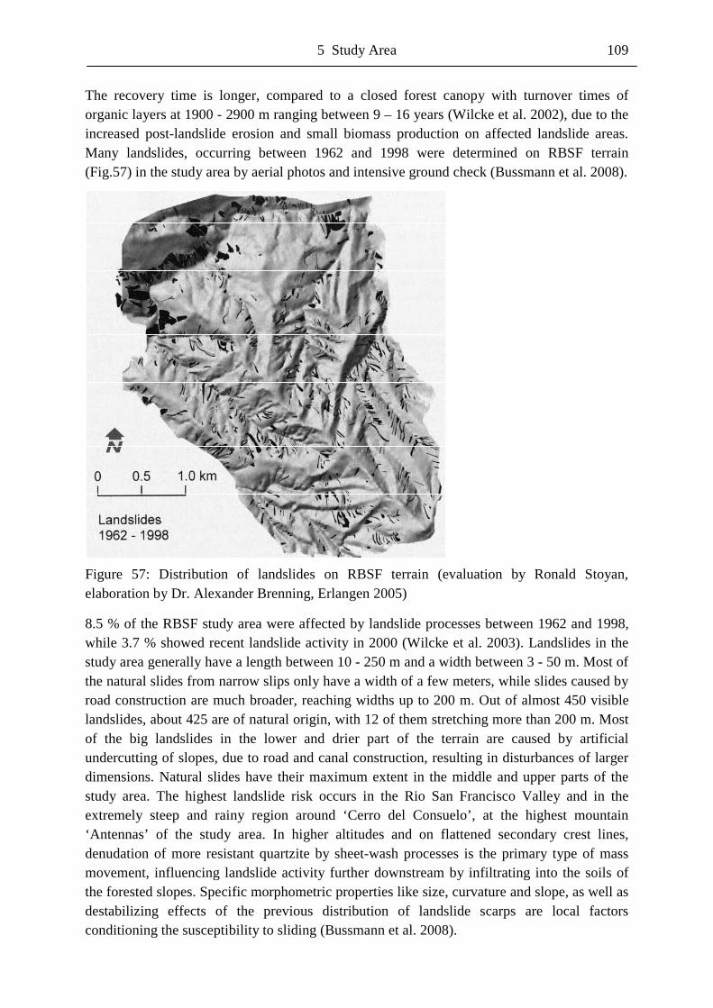
5 Study Area 109

The recovery time is longer, compared to a closed forest canopy with turnover times of organic layers at 1900 - 2900 m ranging between 9 – 16 years (Wilcke et al. 2002), due to the increased post-landslide erosion and small biomass production on affected landslide areas. Many landslides, occurring between 1962 and 1998 were determined on RBSF terrain (Fig.57) in the study area by aerial photos and intensive ground check (Bussmann et al. 2008).

Figure 57: Distribution of landslides on RBSF terrain (evaluation by Ronald Stoyan, elaboration by Dr. Alexander Brenning, Erlangen 2005)

8.5 % of the RBSF study area were affected by landslide processes between 1962 and 1998, while 3.7 % showed recent landslide activity in 2000 (Wilcke et al. 2003). Landslides in the study area generally have a length between 10 - 250 m and a width between 3 - 50 m. Most of the natural slides from narrow slips only have a width of a few meters, while slides caused by road construction are much broader, reaching widths up to 200 m. Out of almost 450 visible landslides, about 425 are of natural origin, with 12 of them stretching more than 200 m. Most of the big landslides in the lower and drier part of the terrain are caused by artificial undercutting of slopes, due to road and canal construction, resulting in disturbances of larger dimensions. Natural slides have their maximum extent in the middle and upper parts of the study area. The highest landslide risk occurs in the Rio San Francisco Valley and in the extremely steep and rainy region around ‘Cerro del Consuelo’, at the highest mountain ‘Antennas’ of the study area. In higher altitudes and on flattened secondary crest lines, denudation of more resistant quartzite by sheet-wash processes is the primary type of mass movement, influencing landslide activity further downstream by infiltrating into the soils of the forested slopes. Specific morphometric properties like size, curvature and slope, as well as destabilizing effects of the previous distribution of landslide scarps are local factors conditioning the susceptibility to sliding (Bussmann et al. 2008).

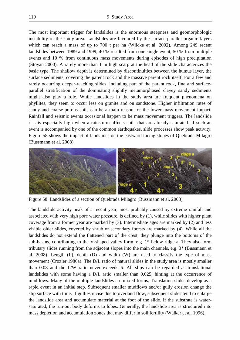
110 5 Study Area

The most important trigger for landslides is the enormous steepness and geomorphologic instability of the study area. Landslides are favoured by the surface-parallel organic layers which can reach a mass of up to 700 t per ha (Wilcke et al. 2002). Among 249 recent landslides between 1989 and 1999, 40 % resulted from one single event, 50 % from multiple events and 10 % from continuous mass movements during episodes of high precipitation (Stoyan 2000). A rarely more than 1 m high scarp at the head of the slide characterizes the basic type. The shallow depth is determined by discontinuities between the humus layer, the surface sediments, covering the parent rock and the massive parent rock itself. For a few and rarely occurring deeper-reaching slides, including part of the parent rock, fine and surface-parallel stratification of the dominating slightly metamorphosed clayey sandy sediments might also play a role. While landslides in the study area are frequent phenomena on phyllites, they seem to occur less on granite and on sandstone. Higher infiltration rates of sandy and coarse-porous soils can be a main reason for the lower mass movement impact. Rainfall and seismic events occasional happen to be mass movement triggers. The landslide risk is especially high when a rainstorm affects soils that are already saturated. If such an event is accompanied by one of the common earthquakes, slide processes show peak activity. Figure 58 shows the impact of landslides on the eastward facing slopes of Quebrada Milagro (Bussmann et al. 2008).

Figure 58: Landslides of a section of Quebrada Milagro (Bussmann et al. 2008)

The landslide activity peak of a recent year, most probably caused by extreme rainfall and associated with very high pore water pressure, is defined by (1), while slides with higher plant coverage from a former year are marked by (3). Intermediate ages are marked by (2) and less visible older slides, covered by shrub or secondary forests are marked by (4). While all the landslides do not extend the flattened part of the crest, they plunge into the bottoms of the sub-basins, contributing to the V-shaped valley form, e.g. 1* below ridge a. They also form tributary slides running from the adjacent slopes into the main channels, e.g. 3* (Bussmann et al. 2008). Length (L), depth (D) and width (W) are used to classify the type of mass movement (Crozier 1986a). The D/L ratio of natural slides in the study area is mostly smaller than 0.08 and the L/W ratio never exceeds 5. All slips can be regarded as translational landslides with some having a D/L ratio smaller than 0.025, hinting at the occurrence of mudflows. Many of the multiple landslides are mixed forms. Translation slides develop as a rapid event in an initial step. Subsequent smaller mudflows and/or gully erosion change the slip surface with time. If gullies incise due to overland flow, subsequent slides tend to enlarge the landslide area and accumulate material at the foot of the slide. If the substrate is water-saturated, the run-out body deforms to lobes. Generally, the landslide area is structured into mass depletion and accumulation zones that may differ in soil fertility (Walker et al. 1996).

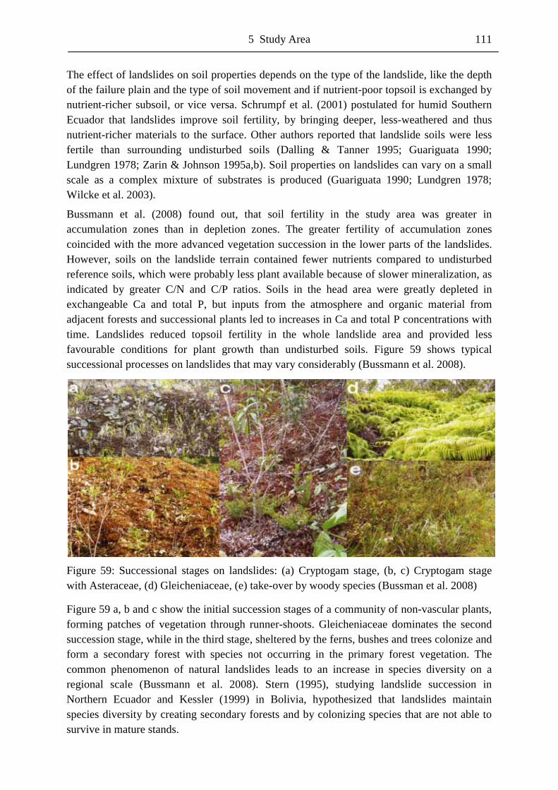
5 Study Area 111

The effect of landslides on soil properties depends on the type of the landslide, like the depth of the failure plain and the type of soil movement and if nutrient-poor topsoil is exchanged by nutrient-richer subsoil, or vice versa. Schrumpf et al. (2001) postulated for humid Southern Ecuador that landslides improve soil fertility, by bringing deeper, less-weathered and thus nutrient-richer materials to the surface. Other authors reported that landslide soils were less fertile than surrounding undisturbed soils (Dalling & Tanner 1995; Guariguata 1990; Lundgren 1978; Zarin & Johnson 1995a,b). Soil properties on landslides can vary on a small scale as a complex mixture of substrates is produced (Guariguata 1990; Lundgren 1978; Wilcke et al. 2003).

Bussmann et al. (2008) found out, that soil fertility in the study area was greater in accumulation zones than in depletion zones. The greater fertility of accumulation zones coincided with the more advanced vegetation succession in the lower parts of the landslides. However, soils on the landslide terrain contained fewer nutrients compared to undisturbed reference soils, which were probably less plant available because of slower mineralization, as indicated by greater C/N and C/P ratios. Soils in the head area were greatly depleted in exchangeable Ca and total P, but inputs from the atmosphere and organic material from adjacent forests and successional plants led to increases in Ca and total P concentrations with time. Landslides reduced topsoil fertility in the whole landslide area and provided less favourable conditions for plant growth than undisturbed soils. Figure 59 shows typical successional processes on landslides that may vary considerably (Bussmann et al. 2008).

Figure 59: Successional stages on landslides: (a) Cryptogam stage, (b, c) Cryptogam stage with Asteraceae, (d) Gleicheniaceae, (e) take-over by woody species (Bussman et al. 2008)

Figure 59 a, b and c show the initial succession stages of a community of non-vascular plants, forming patches of vegetation through runner-shoots. Gleicheniaceae dominates the second succession stage, while in the third stage, sheltered by the ferns, bushes and trees colonize and form a secondary forest with species not occurring in the primary forest vegetation. The common phenomenon of natural landslides leads to an increase in species diversity on a regional scale (Bussmann et al. 2008). Stern (1995), studying landslide succession in Northern Ecuador and Kessler (1999) in Bolivia, hypothesized that landslides maintain species diversity by creating secondary forests and by colonizing species that are not able to survive in mature stands.

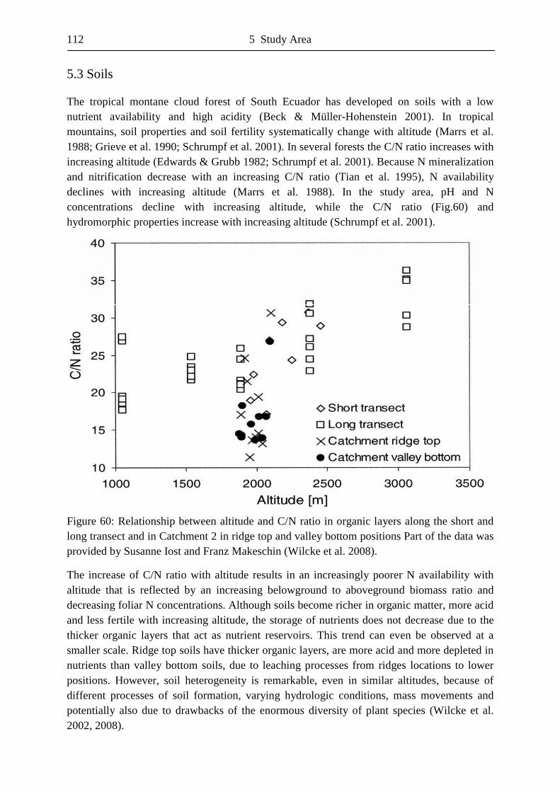
112 5 Study Area

5.3 Soils

The tropical montane cloud forest of South Ecuador has developed on soils with a low nutrient availability and high acidity (Beck & Müller-Hohenstein 2001). In tropical mountains, soil properties and soil fertility systematically change with altitude (Marrs et al. 1988; Grieve et al. 1990; Schrumpf et al. 2001). In several forests the C/N ratio increases with increasing altitude (Edwards & Grubb 1982; Schrumpf et al. 2001). Because N mineralization and nitrification decrease with an increasing C/N ratio (Tian et al. 1995), N availability declines with increasing altitude (Marrs et al. 1988). In the study area, pH and N concentrations decline with increasing altitude, while the C/N ratio (Fig.60) and hydromorphic properties increase with increasing altitude (Schrumpf et al. 2001).

Figure 60: Relationship between altitude and C/N ratio in organic layers along the short and long transect and in Catchment 2 in ridge top and valley bottom positions Part of the data was provided by Susanne Iost and Franz Makeschin (Wilcke et al. 2008).

The increase of C/N ratio with altitude results in an increasingly poorer N availability with altitude that is reflected by an increasing belowground to aboveground biomass ratio and decreasing foliar N concentrations. Although soils become richer in organic matter, more acid and less fertile with increasing altitude, the storage of nutrients does not decrease due to the thicker organic layers that act as nutrient reservoirs. This trend can even be observed at a smaller scale. Ridge top soils have thicker organic layers, are more acid and more depleted in nutrients than valley bottom soils, due to leaching processes from ridges locations to lower positions. However, soil heterogeneity is remarkable, even in similar altitudes, because of different processes of soil formation, varying hydrologic conditions, mass movements and potentially also due to drawbacks of the enormous diversity of plant species (Wilcke et al. 2002, 2008).

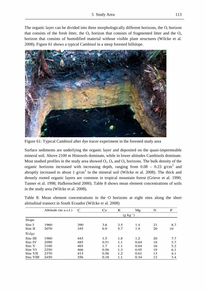
5 Study Area 113

The organic layer can be divided into three morphologically different horizons, the Oi horizon that consists of the fresh litter, the Oe horizon that consists of fragmented litter and the Oa horizon that consists of humidified material without visible plant structures (Wilcke et al. 2008). Figure 61 shows a typical Cambisol in a steep forested hillslope.

Figure 61: Typical Cambisol after dye tracer experiment in the forested study area

Surface sediments are underlying the organic layer and deposited on the quasi-impermeable mineral soil. Above 2100 m Histosols dominate, while in lower altitudes Cambisols dominate. Most studied profiles in the study area showed Oi, Oe and Oa horizons. The bulk density of the organic horizons increased with increasing depth, ranging from 0.08 – 0.23 g/cm3 and abruptly increased to about 1 g/cm3 in the mineral soil (Wilcke et al. 2008). The thick and densely rooted organic layers are common in tropical mountain forest (Grieve et al. 1990; Tanner et al. 1998; Hafkenscheid 2000). Table 8 shows mean element concentrations of soils in the study area (Wilcke et al. 2008).

Table 8: Mean element concentrations in the O horizons at eight sites along the short altitudinal transect in South Ecuador (Wilcke et al. 2008)

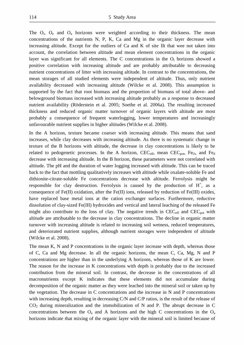
114 5 Study Area

The Oi, Oe and Oa horizons were weighted according to their thickness. The mean concentrations of the nutrients N, P, K, Ca and Mg in the organic layer decrease with increasing altitude. Except for the outliers of Ca and K of site ��t that wee not taken into account, the correlation between altitude and mean element concentrations in the organic layer was significant for all elements. The C concentrations in the Oi horizons showed a positive correlation with increasing altitude and are probably attributable to decreasing nutrient concentrations of litter with increasing altitude. In contrast to the concentrations, the mean storages of all studied elements were independent of altitude. Thus, only nutrient availability decreased with increasing altitude (Wilcke et al. 2008). This assumption is supported by the fact that root biomass and the proportion of biomass of total above- and belowground biomass increased with increasing altitude probably as a response to decreased nutrient availability (Röderstein et al. 2005; Soethe et al. 2006a). The resulting increased thickness and reduced organic matter turnover of organic layers with altitude are most probably a consequence of frequent waterlogging, lower temperatures and increasingly unfavourable nutrient supplies in higher altitudes (Wilcke et al. 2008).

In the A horizon, texture became coarser with increasing altitude. This means that sand increases, while clay decreases with increasing altitude. As there is no systematic change in texture of the B horizons with altitude, the decrease in clay concentrations is likely to be related to pedogenetic processes. In the A horizon, CECeff, mean CECpot, FeO, and Fed decrease with increasing altitude. In the B horizon, these parameters were not correlated with altitude. The pH and the duration of water logging increased with altitude. This can be traced back to the fact that mottling qualitatively increases with altitude while oxalate-soluble Fe and dithionite-citrate-soluble Fe concentrations decrease with altitude. Ferrolysis might be responsible for clay destruction. Ferrolysis is caused by the production of H+, as a consequence of Fe(��) oxidation, after the Fe(��) ions, released by reduction of Fe(���) oxides, have replaced base metal ions at the cation exchanger surfaces. Furthermore, reductive dissolution of clay-sized Fe(���) hydroxides and vertical and lateral leaching of the released Fe might also contribute to the loss of clay. The negative trends in CECeff and CECpot with altitude are attributable to the decrease in clay concentrations. The decline in organic matter turnover with increasing altitude is related to increasing soil wetness, reduced temperatures, and deteriorated nutrient supplies, although nutrient storages were independent of altitude (Wilcke et al. 2008).

The mean K, N and P concentrations in the organic layer increase with depth, whereas those of C, Ca and Mg decrease. In all the organic horizons, the mean C, Ca, Mg, N and P concentrations are higher than in the underlying A horizons, whereas those of K are lower. The reason for the increase in K concentrations with depth is probably due to the increased contribution from the mineral soil. In contrast, the decrease in the concentrations of all macronutrients except K indicates that these elements did not accumulate during decomposition of the organic matter as they were leached into the mineral soil or taken up by the vegetation. The decrease in C concentrations and the increase in N and P concentrations with increasing depth, resulting in decreasing C/N and C/P ratios, is the result of the release of CO2 during mineralization and the immobilization of N and P. The abrupt decrease in C concentrations between the Oa and A horizons and the high C concentrations in the Oa horizons indicate that mixing of the organic layer with the mineral soil is limited because of

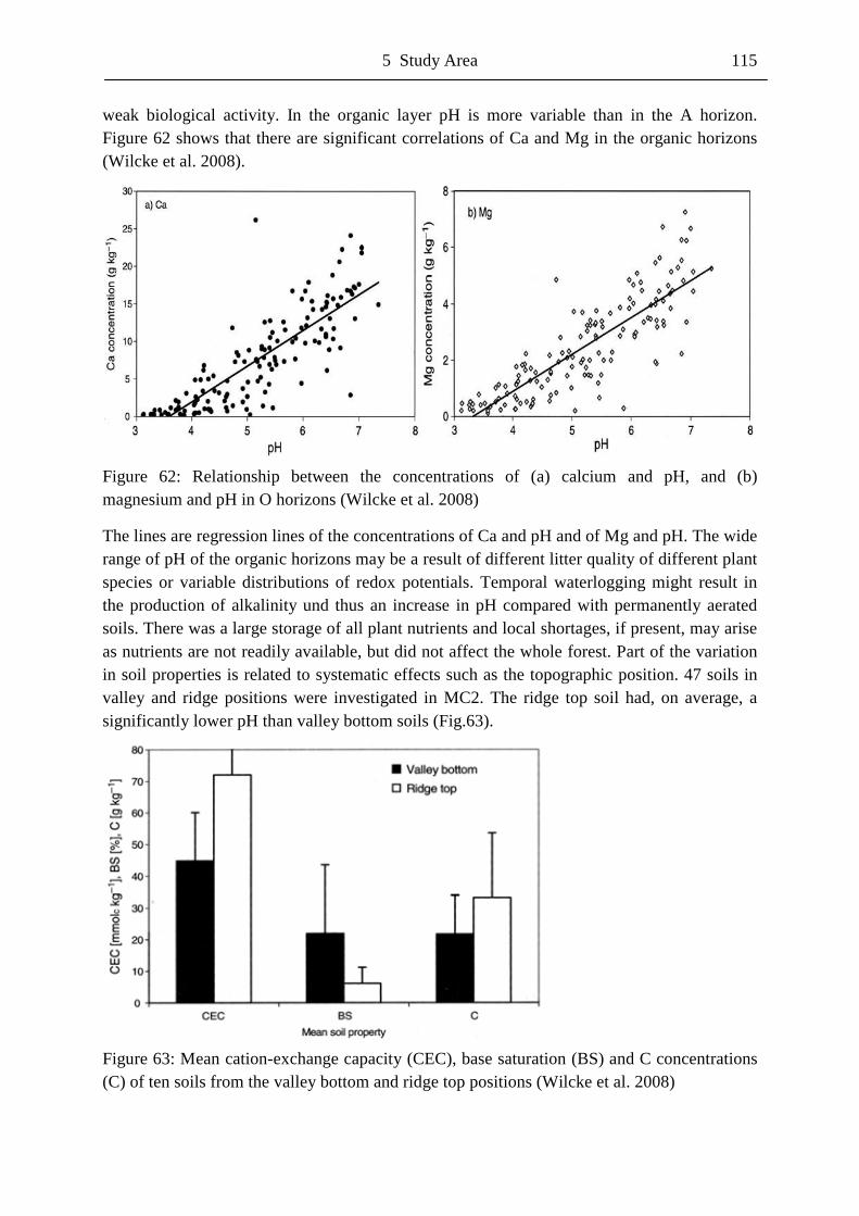
5 Study Area 115

weak biological activity. In the organic layer pH is more variable than in the A horizon. Figure 62 shows that there are significant correlations of Ca and Mg in the organic horizons (Wilcke et al. 2008).

Figure 62: Relationship between the concentrations of (a) calcium and pH, and (b) magnesium and pH in O horizons (Wilcke et al. 2008)

The lines are regression lines of the concentrations of Ca and pH and of Mg and pH. The wide range of pH of the organic horizons may be a result of different litter quality of different plant species or variable distributions of redox potentials. Temporal waterlogging might result in the production of alkalinity und thus an increase in pH compared with permanently aerated soils. There was a large storage of all plant nutrients and local shortages, if present, may arise as nutrients are not readily available, but did not affect the whole forest. Part of the variation in soil properties is related to systematic effects such as the topographic position. 47 soils in valley and ridge positions were investigated in MC2. The ridge top soil had, on average, a significantly lower pH than valley bottom soils (Fig.63).

Figure 63: Mean cation-exchange capacity (CEC), base saturation (BS) and C concentrations (C) of ten soils from the valley bottom and ridge top positions (Wilcke et al. 2008)

116 5 Study Area

Error bars indicate standard deviations. The mean CECeff in the A horizons was significantly higher in ridge top soils than in valley bottom soils, because of the higher organic matter concentration. The mean base saturation in the A horizons was significantly lower in the ridge top soils than in the valley bottom soils. In the valley bottom soils, mean total concentrations of Ca, Mg and P were higher than in the ridge top soils. Enhanced acidification, lower base saturation, and lower total element concentrations of the ridge top than of the valley bottom soils were the result of element leaching from ridge top to valley bottom positions. The reason is probably the higher water input than in the sheltered valley bottom positions, and slightly lower soil temperatures. The spatial variability in soil properties is attributable to differences in climatic conditions but also to the position in the landscape, where water and matter transport occurs from upper to lower areas (Wilcke et al. 2008).

Soil structure, stone content, plant root systems and possibly land use are controlling factors for water flow in soils. The water flow in disturbed and undisturbed tropical soils has been studied with dye tracer experiments, showing that the infiltration depths of the dye varied between the different study sites. While a new landslide and a pasture soil showed a rather simple pattern with a few preferential flow paths, the primary forest site showed a complex pattern. Despite the high irrigation intensity and the high amount of solution applied, the tracer did not exceed a certain depth. Another primary forest soil, as well as an old landslide showed deep infiltration. It was shown that stones create preferential flowpaths and increase flow velocity. Preferential flow results in variable soil moisture distribution and water supply, influencing root growth, C- and N-mineralization, denitrification, humus accumulation, the coexistence of zones with high and low oxidation potential and leads to rapid leaching of nutrients. As the air phase is discontinuous, the oxygen supply of plant roots and microorganisms can be interrupted. Chemical and physico-chemical reactions, such as cation exchange, kinetic sorption processes or nutrient exchange between mobile and immobile water, precipitations and oxidations are also affected by the occurrence of preferential flow (Bogner et al. 2008).

Soils of the open Páramo on the ridge develop on solid rocky layers, which cause long-lasting water stagnation. Thus, moisture content is considerably higher, compared to coarse porous debris layer beyond the forests. Thick humus layers in elfin forests protect the soils from drying up. Thus elfin forests create their own water regime by the mighty upper-most organic stratum that conserves moisture even during the long dry periods of ‘Veranillo del Niño’ events that rarely last longer than two weeks. Furthermore, the immense water storage capacities of thick epiphytic bryophyte packages on tree branches are verified as a general feature of elfin forests (Müller & Frahm 1998; Kürschner & Parolly 2004b).

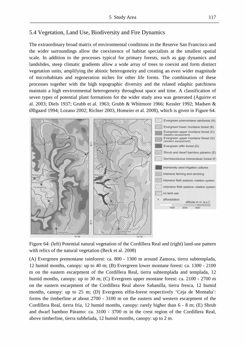
5 Study Area 117

5.4 Vegetation, Land Use, Biodiversity and Fire Dynamics

The extraordinary broad matrix of environmental conditions in the Reserve San Francisco and the wider surroundings allow the coexistence of habitat specialists at the smallest spatial scale. In addition to the processes typical for primary forests, such as gap dynamics and landslides, steep climatic gradients allow a wide array of trees to coexist and form distinct vegetation units, amplifying the abiotic heterogeneity and creating an even wider magnitude of microhabitats and regeneration niches for other life forms. The combination of these processes together with the high topographic diversity and the related edaphic patchiness maintain a high environmental heterogeneity throughout space and time. A classification of seven types of potential plant formations for the wider study area was generated (Aguirre et al. 2003; Diels 1937; Grubb et al. 1963; Grubb & Whitmore 1966; Kessler 1992; Madsen & Øllgaard 1994; Lozano 2002; Richter 2003, Homeier et al. 2008), which is given in Figure 64.

Figure 64: (left) Potential natural vegetation of the Cordillera Real and (right) land-use pattern with relics of the natural vegetation (Beck et al. 2008)

(A) Evergreen premontane rainforest: ca. 800 - 1300 m around Zamora, tierra subtemplada, 12 humid months, canopy: up to 40 m; (B) Evergreen lower montane forest: ca. 1300 - 2100 m on the eastern escarpment of the Cordillera Real, tierra subtemplada and templada, 12 humid months, canopy: up to 30 m; (C) Evergreen upper montane forest: ca. 2100 - 2700 m on the eastern escarpment of the Cordillera Real above Sabanilla, tierra fresca, 12 humid months, canopy: up to 25 m; (D) Evergreen elfin-forest respectively ‘Ceja de Montaña’: forms the timberline at about 2700 - 3100 m on the eastern and western escarpment of the Cordillera Real, tierra fría, 12 humid months, canopy: rarely higher than 6 - 8 m; (E) Shrub and dwarf bamboo Páramo: ca. 3100 - 3700 m in the crest region of the Cordillera Real, above timberline, tierra subhelada, 12 humid months, canopy: up to 2 m.

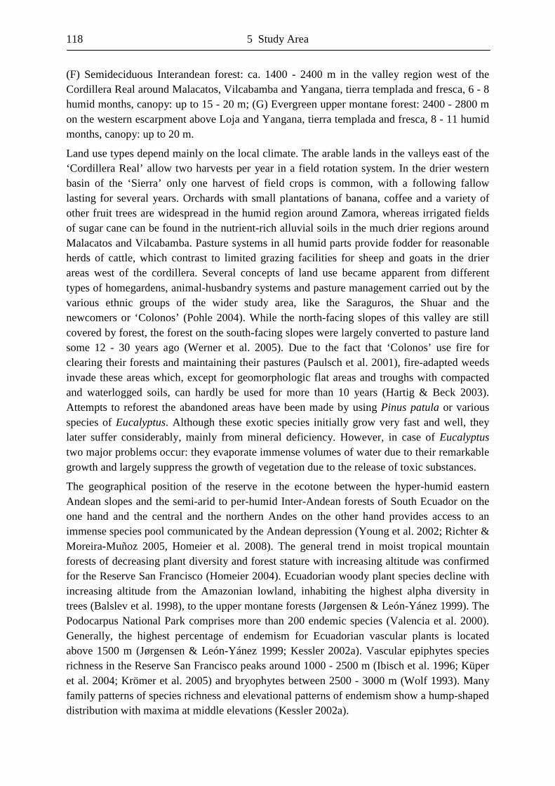
118 5 Study Area

(F) Semideciduous Interandean forest: ca. 1400 - 2400 m in the valley region west of the Cordillera Real around Malacatos, Vilcabamba and Yangana, tierra templada and fresca, 6 - 8 humid months, canopy: up to 15 - 20 m; (G) Evergreen upper montane forest: 2400 - 2800 m on the western escarpment above Loja and Yangana, tierra templada and fresca, 8 - 11 humid months, canopy: up to 20 m.

Land use types depend mainly on the local climate. The arable lands in the valleys east of the ‘Cordillera Real’ allow two harvests per year in a field rotation system. In the drier western basin of the ‘Sierra’ only one harvest of field crops is common, with a following fallow lasting for several years. Orchards with small plantations of banana, coffee and a variety of other fruit trees are widespread in the humid region around Zamora, whereas irrigated fields of sugar cane can be found in the nutrient-rich alluvial soils in the much drier regions around Malacatos and Vilcabamba. Pasture systems in all humid parts provide fodder for reasonable herds of cattle, which contrast to limited grazing facilities for sheep and goats in the drier areas west of the cordillera. Several concepts of land use became apparent from different types of homegardens, animal-husbandry systems and pasture management carried out by the various ethnic groups of the wider study area, like the Saraguros, the Shuar and the newcomers or ‘Colonos’ (Pohle 2004). While the north-facing slopes of this valley are still covered by forest, the forest on the south-facing slopes were largely converted to pasture land some 12 - 30 years ago (Werner et al. 2005). Due to the fact that ‘Colonos’ use fire for clearing their forests and maintaining their pastures (Paulsch et al. 2001), fire-adapted weeds invade these areas which, except for geomorphologic flat areas and troughs with compacted and waterlogged soils, can hardly be used for more than 10 years (Hartig & Beck 2003). Attempts to reforest the abandoned areas have been made by using Pinus patula or various species of Eucalyptus. Although these exotic species initially grow very fast and well, they later suffer considerably, mainly from mineral deficiency. However, in case of Eucalyptus two major problems occur: they evaporate immense volumes of water due to their remarkable growth and largely suppress the growth of vegetation due to the release of toxic substances.

The geographical position of the reserve in the ecotone between the hyper-humid eastern Andean slopes and the semi-arid to per-humid Inter-Andean forests of South Ecuador on the one hand and the central and the northern Andes on the other hand provides access to an immense species pool communicated by the Andean depression (Young et al. 2002; Richter & Moreira-Muñoz 2005, Homeier et al. 2008). The general trend in moist tropical mountain forests of decreasing plant diversity and forest stature with increasing altitude was confirmed for the Reserve San Francisco (Homeier 2004). Ecuadorian woody plant species decline with increasing altitude from the Amazonian lowland, inhabiting the highest alpha diversity in trees (Balslev et al. 1998), to the upper montane forests (Jørgensen & León-Yánez 1999). The Podocarpus National Park comprises more than 200 endemic species (Valencia et al. 2000). Generally, the highest percentage of endemism for Ecuadorian vascular plants is located above 1500 m (Jørgensen & León-Yánez 1999; Kessler 2002a). Vascular epiphytes species richness in the Reserve San Francisco peaks around 1000 - 2500 m (Ibisch et al. 1996; Küper et al. 2004; Krömer et al. 2005) and bryophytes between 2500 - 3000 m (Wolf 1993). Many family patterns of species richness and elevational patterns of endemism show a hump-shaped distribution with maxima at middle elevations (Kessler 2002a).

5 Study Area 119

The forest of the study area consists of the Subtypes (B), (C) and (D) and can more exactly be divided into the following five Forest Types. All following floristic composition profiles have a depth of 5 m and show only trees with a diameter greater than 5 cm. 1) Subtype of (B): Evergreen Lower Montane Forest

The Forest of the Rio San Francisco Valley and Major Ravines below about 2200 m is the tallest and most speciose forest, growing on gentle lower slopes and within major ravines. The canopy attains 20 - 25 m, with emergent reaching up to 35 m. The general appearance of the forest becomes considerably wetter at higher altitudes due to lusher epiphytic vegetation.

Figure 65: Profile diagram of Forest Type 1 at the RBSF (1960 m) 2) Subtype of (B): Evergreen Lower Montane Forest

The Forest along Ridges and Upper Slopes from about 1900 - 2100 m attains heights between 15 - 20 m on slopes and 8 - 10 m on exposed ridges. A characteristic feature of this forest type is the thick raw humus layer.

Figure 66: Profile diagram of Forest Type 2 at the RBSF (2050 m)

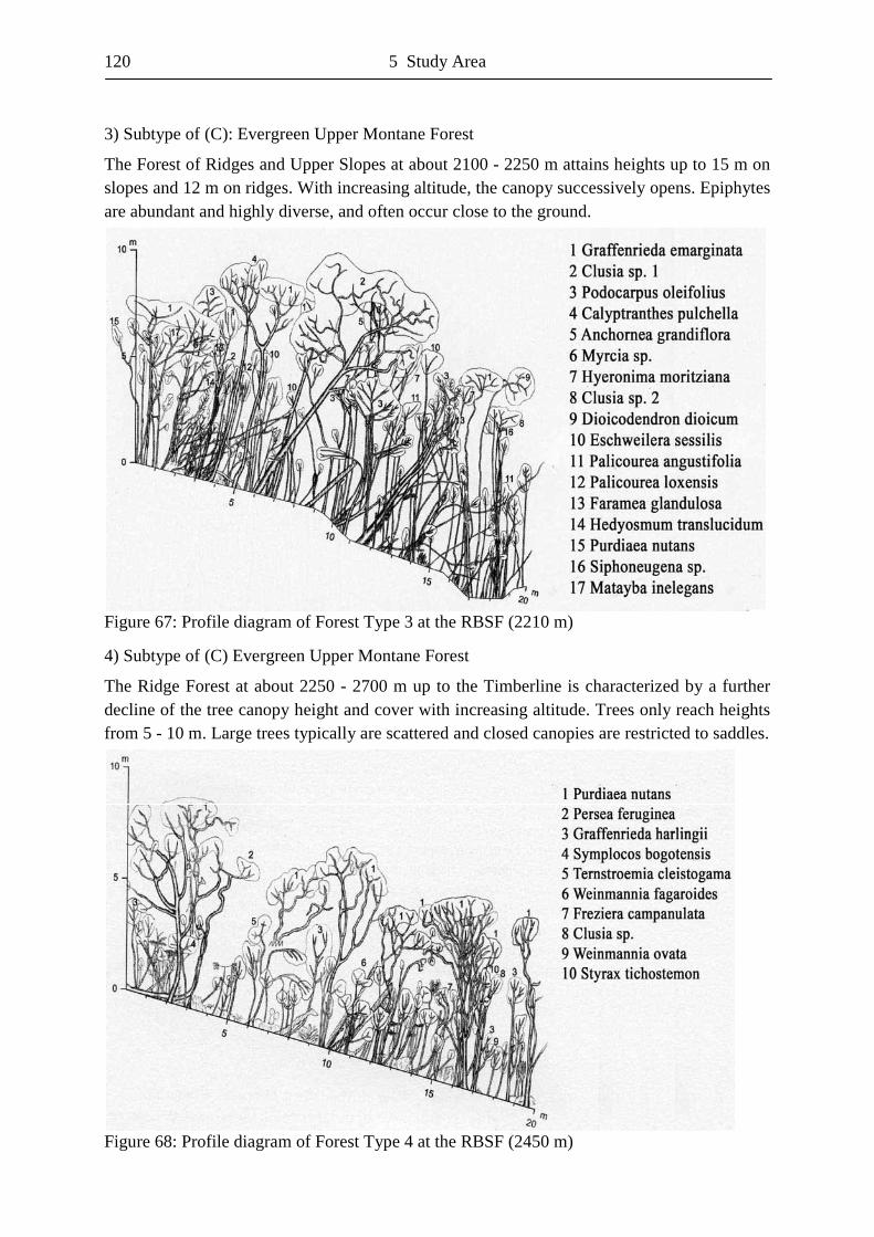
120 5 Study Area

3) Subtype of (C): Evergreen Upper Montane Forest

The Forest of Ridges and Upper Slopes at about 2100 - 2250 m attains heights up to 15 m on slopes and 12 m on ridges. With increasing altitude, the canopy successively opens. Epiphytes are abundant and highly diverse, and often occur close to the ground.

Figure 67: Profile diagram of Forest Type 3 at the RBSF (2210 m) 4) Subtype of (C) Evergreen Upper Montane Forest

The Ridge Forest at about 2250 - 2700 m up to the Timberline is characterized by a further decline of the tree canopy height and cover with increasing altitude. Trees only reach heights from 5 - 10 m. Large trees typically are scattered and closed canopies are restricted to saddles.

Figure 68: Profile diagram of Forest Type 4 at the RBSF (2450 m)

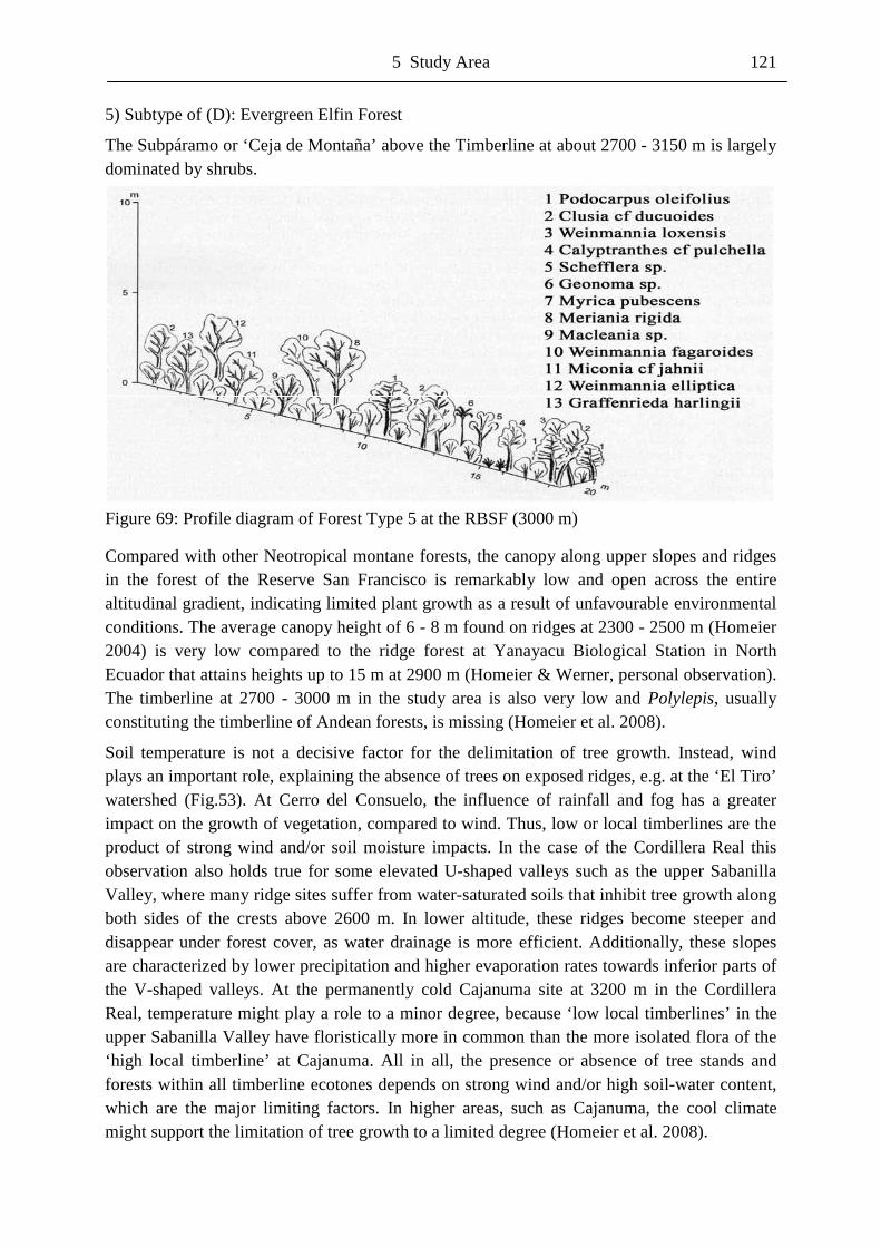
5 Study Area 121

5) Subtype of (D): Evergreen Elfin Forest

The Subpáramo or ‘Ceja de Montaña’ above the Timberline at about 2700 - 3150 m is largely dominated by shrubs.

Figure 69: Profile diagram of Forest Type 5 at the RBSF (3000 m)

Compared with other Neotropical montane forests, the canopy along upper slopes and ridges in the forest of the Reserve San Francisco is remarkably low and open across the entire altitudinal gradient, indicating limited plant growth as a result of unfavourable environmental conditions. The average canopy height of 6 - 8 m found on ridges at 2300 - 2500 m (Homeier 2004) is very low compared to the ridge forest at Yanayacu Biological Station in North Ecuador that attains heights up to 15 m at 2900 m (Homeier & Werner, personal observation). The timberline at 2700 - 3000 m in the study area is also very low and Polylepis, usually constituting the timberline of Andean forests, is missing (Homeier et al. 2008).

Soil temperature is not a decisive factor for the delimitation of tree growth. Instead, wind plays an important role, explaining the absence of trees on exposed ridges, e.g. at the ‘El Tiro’ watershed (Fig.53). At Cerro del Consuelo, the influence of rainfall and fog has a greater impact on the growth of vegetation, compared to wind. Thus, low or local timberlines are the product of strong wind and/or soil moisture impacts. In the case of the Cordillera Real this observation also holds true for some elevated U-shaped valleys such as the upper Sabanilla Valley, where many ridge sites suffer from water-saturated soils that inhibit tree growth along both sides of the crests above 2600 m. In lower altitude, these ridges become steeper and disappear under forest cover, as water drainage is more efficient. Additionally, these slopes are characterized by lower precipitation and higher evaporation rates towards inferior parts of the V-shaped valleys. At the permanently cold Cajanuma site at 3200 m in the Cordillera Real, temperature might play a role to a minor degree, because ‘low local timberlines’ in the upper Sabanilla Valley have floristically more in common than the more isolated flora of the ‘high local timberline’ at Cajanuma. All in all, the presence or absence of tree stands and forests within all timberline ecotones depends on strong wind and/or high soil-water content, which are the major limiting factors. In higher areas, such as Cajanuma, the cool climate might support the limitation of tree growth to a limited degree (Homeier et al. 2008).

122 5 Study Area

Anthropogenic influences and biodiversity:

Anthropogenic influenced areas in the study area are abandoned pastures, farming areas and areas, where the natural forest has been destroyed. However, along trails of active pastures, where fire has not been used for forest clearing, a succession similar to natural landslides can be observed (Ohl & Bussmann 2004). Conforming to the key species concept, all types of secondary forest are characterized by representatives of Chusquea that mainly occurs as tall lianas, but also as bushes or trailing herbs. In agreement with the moderate disturbance theory such secondary forests are extremely rich in plant species and specific groups of animals. Ecotones at tropical forest margins are often very biodiverse habitats, due to their high niche heterogeneity (Ricketts et al. 2001). At lower altitudes, forest types under human influence and succession stages are extraordinary rich in bird species. As a consequence of the ongoing habitat conversions, succession stages, secondary forests and forest remnants are becoming ever more important for the conservation of tropical biodiversity. Generally, the succession leads to a mainly non-linear increase in biodiversity, resulting in decreasing significance of earlier key species (Beck et al. 2008). In contrast, in the study area a few key species dominate and determine the course of the successional process (Hartig & Beck 2003). In areas of abandoned pastures, where fire is used for pasture maintenance, the very aggressive bracken fern Pteridium arachnoideum takes over. The competitive strength of this fern is enhanced by each burning, due to its practically invulnerable subterranean network of rhizomes from which new leaves are produced after a fire. Its big leaves rapidly form closed canopies and thus widely suppress upcoming seedlings of other plant species.

The steep slopes allow light to reach the ground, so that ubiquitous seeds of a few weedy bush species can germinate, grow and penetrate the fern canopy. These bushes are mainly Asteraceae, Ericaceae and Melastomataceae, which are all characterized by an enormous seed production. Together with the bracken fern, they form a stable plant community so that the invasion by trees is very unlikely. Once bracken fern has taken over, recultivation of the area is extremely difficult. Continued cutting of the fronds combined with the application of herbicides is expensive and needs to be continued for years until the rhizomes die (Marrs et al. 1998). In contrast to the regeneration of the forest on small-scale clearings the wide abandoned areas are poor in animal species, as neither bracken fern nor the bushes are attractive fodder plants for herbivores.

Prance (1973) has identified eastern Ecuador as the possible site of a Pleistocene refuge forest. Physical geographers theorize that eastern Ecuador remained forested when climatic changes caused a generalized reduction in the extent of tropical forests during the Pleistocene. The extraordinary age of the forests should promote endemism, which in turn would lead to extraordinary levels of species diversity in places like eastern Ecuador. Although its land area is only slightly larger than the state of Colorado, Ecuador has about 20.000 - 25.000 plant species, more than whole North America with about 17.000 plant species, and more animal species with about 2436 than the United States with 1394 animal species. Because the vast majority of these plants and animals live in Ecuador’s rain forests, the continued destruction of these forests causes massive species extinctions (Cabarle et al. 1989).

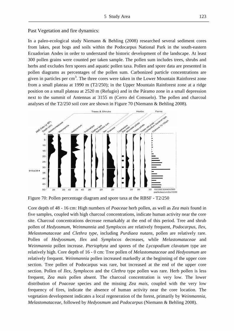
5 Study Area 123

Past Vegetation and fire dynamics:

In a paleo-ecological study Niemann & Behling (2008) researched several sediment cores from lakes, peat bogs and soils within the Podocarpus National Park in the south-eastern Ecuadorian Andes in order to understand the historic development of the landscape. At least 300 pollen grains were counted per taken sample. The pollen sum includes trees, shrubs and herbs and excludes fern spores and aquatic pollen taxa. Pollen and spore data are presented in pollen diagrams as percentages of the pollen sum. Carbonized particle concentrations are given in particles per cm3. The three cores were taken in the Lower Mountain Rainforest zone from a small plateau at 1990 m (T2/250); in the Upper Mountain Rainforest zone at a ridge position on a small plateau at 2520 m (Refugio) and in the Páramo zone in a small depression next to the summit of Antennas at 3155 m (Cerro del Consuelo). The pollen and charcoal analyses of the T2/250 soil core are shown in Figure 70 (Niemann & Behling 2008).

Figure 70: Pollen percentage diagram and spore taxa at the RBSF - T2/250

Core depth of 48 - 16 cm: High numbers of Poaceae herb pollen, as well as Zea mais found in five samples, coupled with high charcoal concentrations, indicate human activity near the core site. Charcoal concentrations decrease remarkably at the end of this period. Tree and shrub pollen of Hedyosmum, Weinmannia and Symplocos are relatively frequent, Podocarpus, Ilex, Melastomataceae and Clethra type, including Purdiaea nutans, pollen are relatively rare. Pollen of Hedyosmum, Ilex and Symplocos decreases, while Melastomataceae and Weinmannia pollen increase. Pteriophyta and spores of the Lycopodium clavatum type are relatively high. Core depth of 16 - 0 cm: Tree pollen of Melastomataceae and Hedyosmum are relatively frequent. Weinmannia pollen increased markedly at the beginning of the upper core section. Tree pollen of Podocarpus was rare, but increased at the end of the upper core section. Pollen of Ilex, Symplocos and the Clethra type pollen was rare. Herb pollen is less frequent, Zea mais pollen absent. The charcoal concentration is very low. The lower distribution of Poaceae species and the missing Zea mais, coupled with the very low frequency of fires, indicate the absence of human activity near the core location. The vegetation development indicates a local regeneration of the forest, primarily by Weinmannia, Melastomataceae, followed by Hedyosmum and Podocarpus (Niemann & Behling 2008).

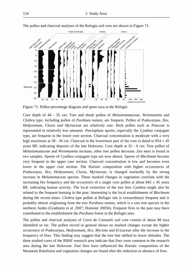
124 5 Study Area

The pollen and charcoal analyses of the Refugio soil core are shown in Figure 71.

Figure 71: Pollen percentage diagram and spore taxa at the Refugio

Core depth of 44 - 35 cm: Tree and shrub pollen of Melastomataceae, Weinmannia and Clethra type, including pollen of Purdiaea nutans, are frequent. Pollen of Podocarpus, Ilex, Hedyosmum, Clusia and Myrtaceae are relatively rare. Herb pollen such as Poaceae is represented in relatively low amounts. Pteriophyta spores, especially the Cyathea conjugate type, are frequent in the lower core section. Charcoal concentration is moderate with a very high maximum at 38 - 36 cm. Charcoal in the lowermost part of the core is dated to 854 ± 45 years BP, indicating deposits of the late Holocene. Core depth at 35 - 0 cm: Tree pollen of Melastomataceae and Weinmannia increase, other tree pollen decrease. Zea mais is found in two samples. Spores of Cyathea conjugate type are now absent. Spores of Blechnum become very frequent in the upper core section. Charcoal concentration is low and becomes even lower in the upper core section. The floristic composition with higher occurrences of Podocarpus, Ilex, Hedyosmum, Clusia, Myrtaceae, is changed markedly by the strong increase in Melastomaceae species. These marked changes in vegetation correlate with the increasing fire frequency and the occurrence of a single corn pollen at about 845 ± 45 years BP, indicating human activity. The local extinction of the tree fern Cyathea might also be related to the frequent burning in the past. Interesting is the local establishment of Blechnum during the recent times. Clethra type pollen at Refugio site is extraordinary frequent and is probably almost originating from the tree Purdiaea nutans, which is a rare tree species in the northern Andes (Gradstein et al. 2007; Homeier 2005b). Frequent fires in the past may have contributed to the establishment the Purdiaea forest in the Refugio area.

The pollen and charcoal analyses of Cerro de Consuelo soil core consist of about 88 taxa identified so far. The pollen record in general shows no marked changes except the higher occurrence of Podocarpus, Hedyosmum, Ilex, Myrsine and Ericaceae after the increase in the frequency of fires. This finding may suggest that the tree line shifted to lower altitudes. The three studied cores of the RBSF research area indicate that fires were common in the research area during the late Holocene. Past fires have influenced the floristic composition of the Mountain Rainforest and vegetation changes are found after the reduction or absence of fires.

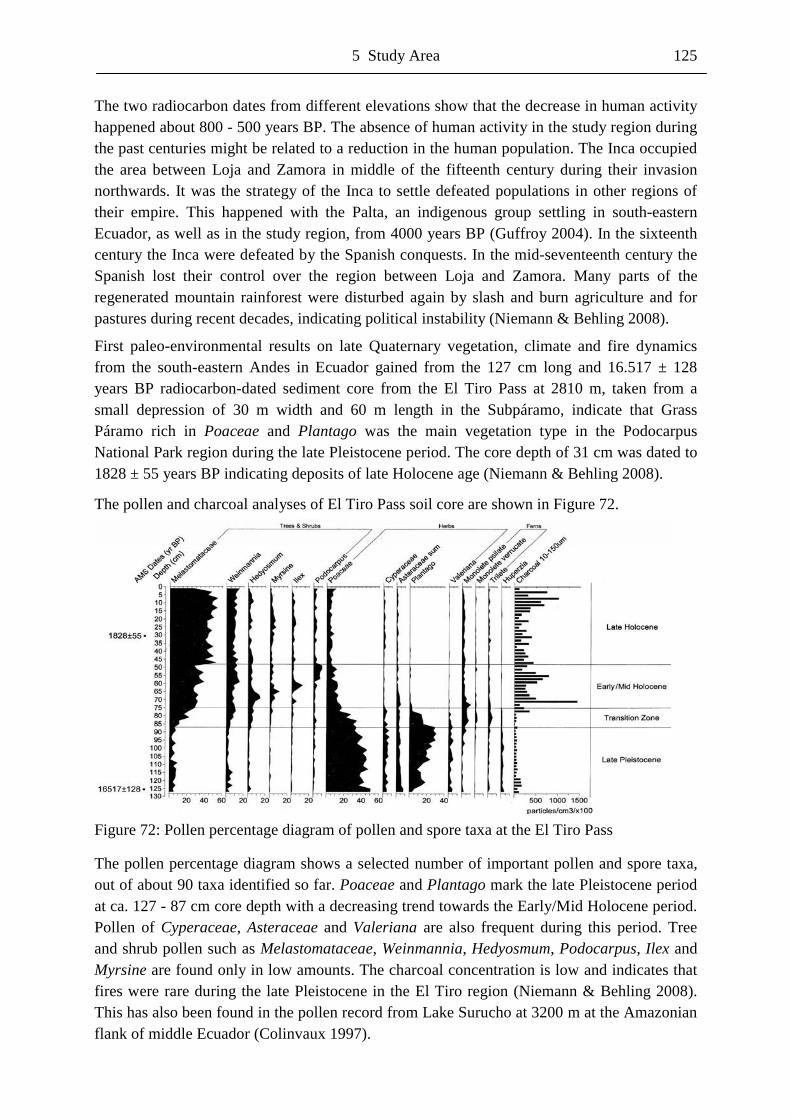
5 Study Area 125

The two radiocarbon dates from different elevations show that the decrease in human activity happened about 800 - 500 years BP. The absence of human activity in the study region during the past centuries might be related to a reduction in the human population. The Inca occupied the area between Loja and Zamora in middle of the fifteenth century during their invasion northwards. It was the strategy of the Inca to settle defeated populations in other regions of their empire. This happened with the Palta, an indigenous group settling in south-eastern Ecuador, as well as in the study region, from 4000 years BP (Guffroy 2004). In the sixteenth century the Inca were defeated by the Spanish conquests. In the mid-seventeenth century the Spanish lost their control over the region between Loja and Zamora. Many parts of the regenerated mountain rainforest were disturbed again by slash and burn agriculture and for pastures during recent decades, indicating political instability (Niemann & Behling 2008).

First paleo-environmental results on late Quaternary vegetation, climate and fire dynamics from the south-eastern Andes in Ecuador gained from the 127 cm long and 16.517 ± 128 years BP radiocarbon-dated sediment core from the El Tiro Pass at 2810 m, taken from a small depression of 30 m width and 60 m length in the Subpáramo, indicate that Grass Páramo rich in Poaceae and Plantago was the main vegetation type in the Podocarpus National Park region during the late Pleistocene period. The core depth of 31 cm was dated to 1828 ± 55 years BP indicating deposits of late Holocene age (Niemann & Behling 2008). The pollen and charcoal analyses of El Tiro Pass soil core are shown in Figure 72.

Figure 72: Pollen percentage diagram of pollen and spore taxa at the El Tiro Pass

The pollen percentage diagram shows a selected number of important pollen and spore taxa, out of about 90 taxa identified so far. Poaceae and Plantago mark the late Pleistocene period at ca. 127 - 87 cm core depth with a decreasing trend towards the Early/Mid Holocene period. Pollen of Cyperaceae, Asteraceae and Valeriana are also frequent during this period. Tree and shrub pollen such as Melastomataceae, Weinmannia, Hedyosmum, Podocarpus, Ilex and Myrsine are found only in low amounts. The charcoal concentration is low and indicates that fires were rare during the late Pleistocene in the El Tiro region (Niemann & Behling 2008). This has also been found in the pollen record from Lake Surucho at 3200 m at the Amazonian flank of middle Ecuador (Colinvaux 1997).

126 5 Study Area

A marked increase of tree and shrub pollen of Melastomataceae, Weinmannia, Hedyosmum and a decrease of herb pollen, especially Poaceae, Cyperaceae, Asteraceae, Valeriana and Plantago are observed during the transition of the late Pleistocene to the Holocene period at ca. 87 - 75 cm core depth, whereas charcoal concentration increases little. Monolete and trilete Pteriophyta spores increases and Huperzia decreases at the end of this period (Niemann & Behling 2008). The pollen record of Laguna Chorrereas at 3700 m report a decrease in Huperzia sp. spores during the transition of the late Pleistocene-Holocene period. Huperzia sp. and Lycopodium sp. characterize the upper cold wet Páramo (Hansen et al. 2003).

It is possible that, during the early to mid-Holocene period at approximate 75 - 48 cm core depth, an Upper Mountain Rainforest vegetation type developed at the study site, suggested by the increasing succession stages of Melastomataceae, Weinmannia, Hedyosmum, Myrsine, Ilex and Podocarpus and the stronger decomposition of organic material during this period that suggest a warmer climate than today. Monolete and trilete Pteriophyta spores decreases at the beginning of this period. Charcoal concentration increases markedly, indicating that fires became quite frequent during this period (Niemann & Behling 2008). However, first human activity in the region of Loja is dated by around 4000 years BP (Guffroy 2004), but human activities may have occurred in the dry Inter-Andean valley much earlier. In the Sabana de Bogota in Colombia, Amerindians were persent from 12500 years BP onward and possibly even before that time (Van der Hammen & Correal Urrego 1978). The modern Subpáramo vegetation became established during the mid- to late Holocene period at the El Tiro Pass. At ca. 48 – 0 cm Melastomataceae pollen become dominant, while other tree and shrub pollen taxa such as of Hedyosmum, Myrsine, Ilex and Podocarpus are slightly less frequent. However, the pollen data suggest the formation of a relatively stable Subpáramo vegetation of the study site since that time (Niemann & Behling 2008).

Fires were rare during the late Pleistocene, remain frequent during the mid-Holocene period and become more frequent during the late Holocene, before decreasing in the very late Holocene in the El Tiro region, suggesting an increase of human activities near or at the El Tiro slopes. The pollen record from Lake Surucucho (3200 m), at the Amazonian flank of middle Ecuador, shows a strong increase of fires during the late Holocene (Colinvaux 1997). This may suggest that the increase of fire frequency in the El Tiro Pass record derives from human activity. The comparison with other Ecuadorian records suggests that the fires are of anthropogenic origin (Niemann & Behling 2008).

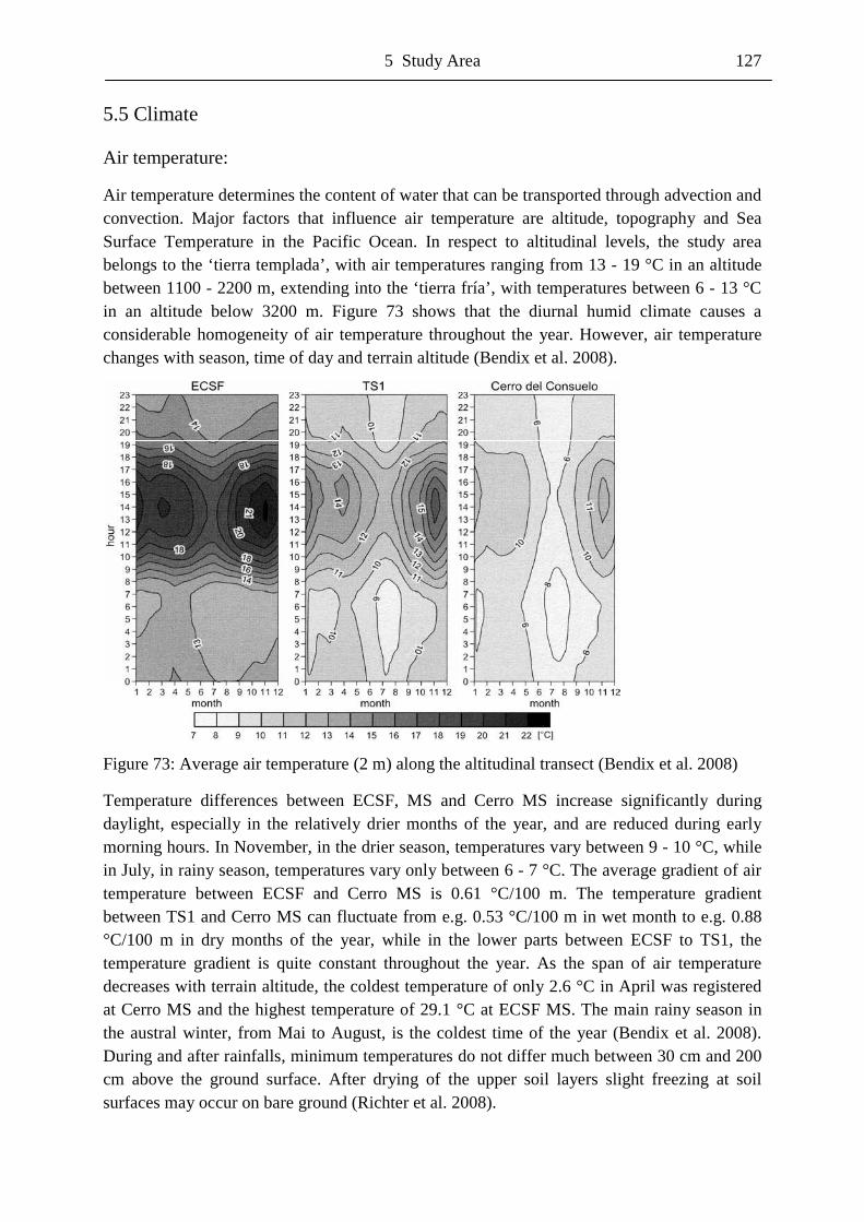
5 Study Area 127

5.5 Climate Air temperature:

Air temperature determines the content of water that can be transported through advection and convection. Major factors that influence air temperature are altitude, topography and Sea Surface Temperature in the Pacific Ocean. In respect to altitudinal levels, the study area belongs to the ‘tierra templada’, with air temperatures ranging from 13 - 19 °C in an altitude between 1100 - 2200 m, extending into the ‘tierra fría’, with temperatures between 6 - 13 °C in an altitude below 3200 m. Figure 73 shows that the diurnal humid climate causes a considerable homogeneity of air temperature throughout the year. However, air temperature changes with season, time of day and terrain altitude (Bendix et al. 2008).

Figure 73: Average air temperature (2 m) along the altitudinal transect (Bendix et al. 2008)

Temperature differences between ECSF, MS and Cerro MS increase significantly during daylight, especially in the relatively drier months of the year, and are reduced during early morning hours. In November, in the drier season, temperatures vary between 9 - 10 °C, while in July, in rainy season, temperatures vary only between 6 - 7 °C. The average gradient of air temperature between ECSF and Cerro MS is 0.61 °C/100 m. The temperature gradient between TS1 and Cerro MS can fluctuate from e.g. 0.53 °C/100 m in wet month to e.g. 0.88 °C/100 m in dry months of the year, while in the lower parts between ECSF to TS1, the temperature gradient is quite constant throughout the year. As the span of air temperature decreases with terrain altitude, the coldest temperature of only 2.6 °C in April was registered at Cerro MS and the highest temperature of 29.1 °C at ECSF MS. The main rainy season in the austral winter, from Mai to August, is the coldest time of the year (Bendix et al. 2008). During and after rainfalls, minimum temperatures do not differ much between 30 cm and 200 cm above the ground surface. After drying of the upper soil layers slight freezing at soil surfaces may occur on bare ground (Richter et al. 2008).

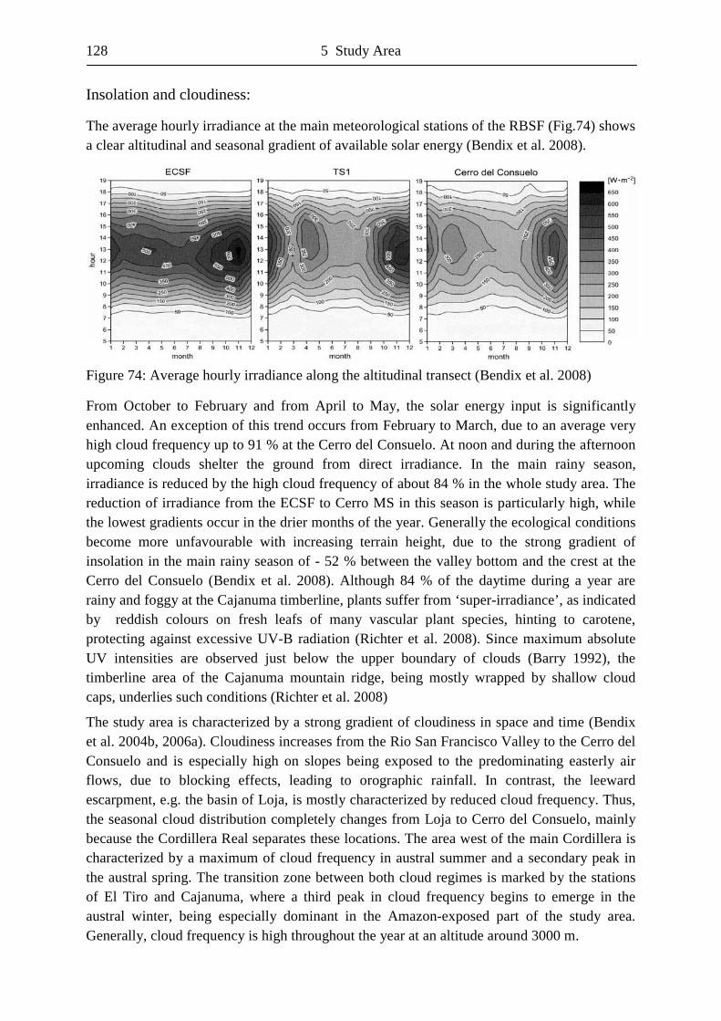
128 5 Study Area

Insolation and cloudiness:

The average hourly irradiance at the main meteorological stations of the RBSF (Fig.74) shows a clear altitudinal and seasonal gradient of available solar energy (Bendix et al. 2008).

Figure 74: Average hourly irradiance along the altitudinal transect (Bendix et al. 2008)

From October to February and from April to May, the solar energy input is significantly enhanced. An exception of this trend occurs from February to March, due to an average very high cloud frequency up to 91 % at the Cerro del Consuelo. At noon and during the afternoon upcoming clouds shelter the ground from direct irradiance. In the main rainy season, irradiance is reduced by the high cloud frequency of about 84 % in the whole study area. The reduction of irradiance from the ECSF to Cerro MS in this season is particularly high, while the lowest gradients occur in the drier months of the year. Generally the ecological conditions become more unfavourable with increasing terrain height, due to the strong gradient of insolation in the main rainy season of - 52 % between the valley bottom and the crest at the Cerro del Consuelo (Bendix et al. 2008). Although 84 % of the daytime during a year are rainy and foggy at the Cajanuma timberline, plants suffer from ‘super-irradiance’, as indicated by reddish colours on fresh leafs of many vascular plant species, hinting to carotene, protecting against excessive UV-B radiation (Richter et al. 2008). Since maximum absolute UV intensities are observed just below the upper boundary of clouds (Barry 1992), the timberline area of the Cajanuma mountain ridge, being mostly wrapped by shallow cloud caps, underlies such conditions (Richter et al. 2008)

The study area is characterized by a strong gradient of cloudiness in space and time (Bendix et al. 2004b, 2006a). Cloudiness increases from the Rio San Francisco Valley to the Cerro del Consuelo and is especially high on slopes being exposed to the predominating easterly air flows, due to blocking effects, leading to orographic rainfall. In contrast, the leeward escarpment, e.g. the basin of Loja, is mostly characterized by reduced cloud frequency. Thus, the seasonal cloud distribution completely changes from Loja to Cerro del Consuelo, mainly because the Cordillera Real separates these locations. The area west of the main Cordillera is characterized by a maximum of cloud frequency in austral summer and a secondary peak in the austral spring. The transition zone between both cloud regimes is marked by the stations of El Tiro and Cajanuma, where a third peak in cloud frequency begins to emerge in the austral winter, being especially dominant in the Amazon-exposed part of the study area. Generally, cloud frequency is high throughout the year at an altitude around 3000 m.

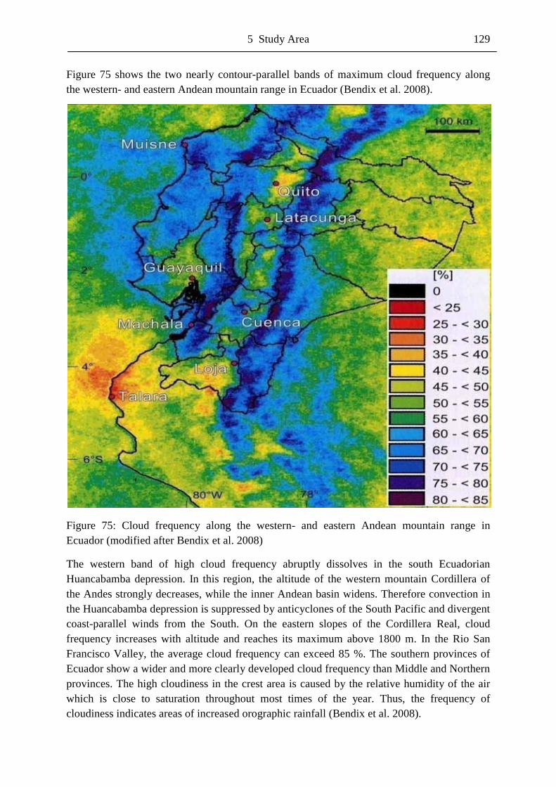
5 Study Area 129

Figure 75 shows the two nearly contour-parallel bands of maximum cloud frequency along the western- and eastern Andean mountain range in Ecuador (Bendix et al. 2008).

Figure 75: Cloud frequency along the western- and eastern Andean mountain range in Ecuador (modified after Bendix et al. 2008)

The western band of high cloud frequency abruptly dissolves in the south Ecuadorian Huancabamba depression. In this region, the altitude of the western mountain Cordillera of the Andes strongly decreases, while the inner Andean basin widens. Therefore convection in the Huancabamba depression is suppressed by anticyclones of the South Pacific and divergent coast-parallel winds from the South. On the eastern slopes of the Cordillera Real, cloud frequency increases with altitude and reaches its maximum above 1800 m. In the Rio San Francisco Valley, the average cloud frequency can exceed 85 %. The southern provinces of Ecuador show a wider and more clearly developed cloud frequency than Middle and Northern provinces. The high cloudiness in the crest area is caused by the relative humidity of the air which is close to saturation throughout most times of the year. Thus, the frequency of cloudiness indicates areas of increased orographic rainfall (Bendix et al. 2008).

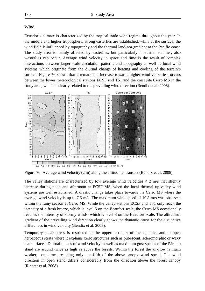
130 5 Study Area

Wind:

Ecuador’s climate is characterized by the tropical trade wind regime throughout the year. In the middle and higher troposphere, strong easterlies are established, while at the surface, the wind field is influenced by topography and the thermal land-sea gradient at the Pacific coast. The study area is mainly affected by easterlies, but particularly in austral summer, also westerlies can occur. Average wind velocity in space and time is the result of complex interactions between larger-scale circulation patterns and topography as well as local wind systems which originate from the diurnal change of heating and cooling of the terrain’s surface. Figure 76 shows that a remarkable increase towards higher wind velocities, occurs between the lower meteorological stations ECSF and TS1 and the crest site Cerro MS in the study area, which is clearly related to the prevailing wind direction (Bendix et al. 2008).

Figure 76: Average wind velocity (2 m) along the altitudinal transect (Bendix et al. 2008)

The valley stations are characterized by low average wind velocities < 2 m/s that slightly increase during noon and afternoon at ECSF MS, when the local thermal up-valley wind systems are well established. A drastic change takes place towards the Cerro MS where the average wind velocity is up to 7.5 m/s. The maximum wind speed of 19.8 m/s was observed within the rainy season at Cerro MS. While the valley stations ECSF and TS1 only reach the intensity of a fresh breeze, which is level 5 on the Beaufort scale, the Cerro MS occasionally reaches the intensity of stormy winds, which is level 8 on the Beaufort scale. The altitudinal gradient of the prevailing wind direction clearly shows the dynamic cause for the distinctive differences in wind velocity (Bendix et al. 2008).

Temporary shear stress is restricted to the uppermost part of the canopies and to open herbaceous strata where it explains xeric structures such as pubescent, scleromorphic or waxy leaf surfaces. Diurnal means of wind velocity as well as maximum gust speeds of the Páramo stand are around twice as high as above the forests. Within the forest the air-flow is much weaker, sometimes reaching only one-fifth of the above-canopy wind speed. The wind direction in open stand differs considerably from the direction above the forest canopy (Richter et al. 2008).

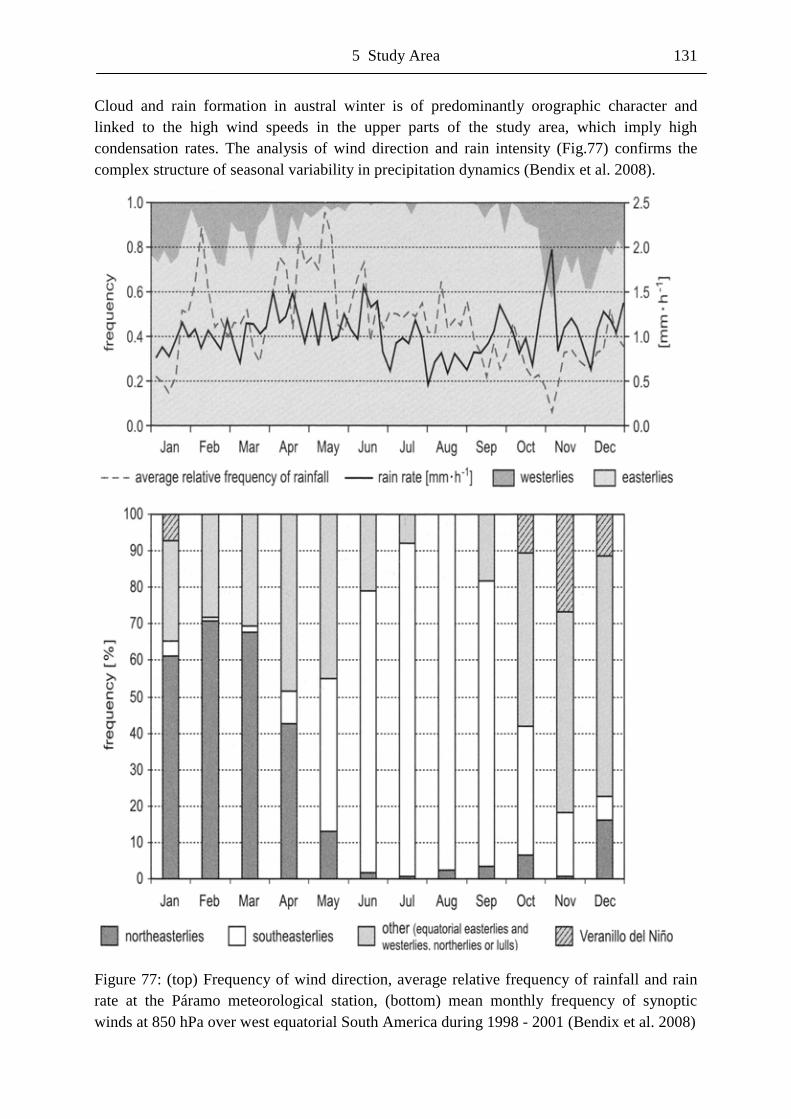
5 Study Area 131

Cloud and rain formation in austral winter is of predominantly orographic character and linked to the high wind speeds in the upper parts of the study area, which imply high condensation rates. The analysis of wind direction and rain intensity (Fig.77) confirms the complex structure of seasonal variability in precipitation dynamics (Bendix et al. 2008).

Figure 77: (top) Frequency of wind direction, average relative frequency of rainfall and rain rate at the Páramo meteorological station, (bottom) mean monthly frequency of synoptic winds at 850 hPa over west equatorial South America during 1998 - 2001 (Bendix et al. 2008)

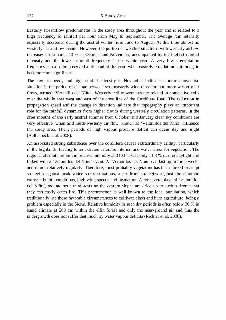
132 5 Study Area

Easterly streamflow predominates in the study area throughout the year and is related to a high frequency of rainfall per hour from May to September. The average rain intensity especially decreases during the austral winter from June to August. At this time almost no westerly streamflow occurs. However, the portion of weather situations with westerly airflow increases up to about 40 % in October and November, accompanied by the highest rainfall intensity and the lowest rainfall frequency in the whole year. A very low precipitation frequency can also be observed at the end of the year, when easterly circulation pattern again become more significant.

The low frequency and high rainfall intensity in November indicates a more convective situation in the period of change between southeasterly wind direction and more westerly air flows, termed ‘Veranillo del Niño’. Westerly cell movements are related to convective cells over the whole area west and east of the crest line of the Cordillera Real. The reduction in propagation speed and the change in direction indicate that topography plays an important role for the rainfall dynamics from higher clouds during westerly circulation patterns. In the drier months of the early austral summer from October and January clear sky conditions are very effective, when arid north-westerly air flow, known as ‘Veranillos del Niño’ influence the study area. Then, periods of high vapour pressure deficit can occur day and night (Rollenbeck et al. 2008).

An associated strong subsidence over the cordillera causes extraordinary aridity, particularly in the highlands, leading to an extreme saturation deficit and water stress for vegetation. The regional absolute minimum relative humidity at 3400 m was only 11.8 % during daylight and linked with a ‘Veranillos del Niño’ event. A ‘Veranillos del Nino’ can last up to three weeks and return relatively regularly. Therefore, most probably vegetation has been forced to adapt strategies against peak water stress situations, apart from strategies against the common extreme humid conditions, high wind speeds and insolation. After several days of ‘Veranillos del Niño’, mountainous rainforests on the eastern slopes are dried up to such a degree that they can easily catch fire. This phenomenon is well-known to the local population, which traditionally use these favorable circumstances to cultivate slash and burn agriculture, being a problem especially in the Sierra. Relative humidity in such dry periods is often below 30 % in stand climate at 200 cm within the elfin forest and only the near-ground air and thus the undergrowth does not suffer that much by water vapour deficits (Richter et al. 2008).

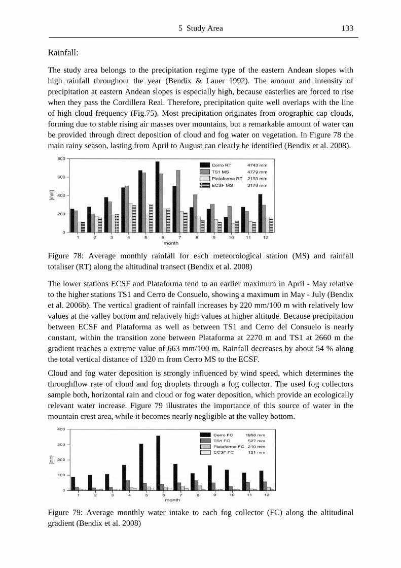
5 Study Area 133

Rainfall:

The study area belongs to the precipitation regime type of the eastern Andean slopes with high rainfall throughout the year (Bendix & Lauer 1992). The amount and intensity of precipitation at eastern Andean slopes is especially high, because easterlies are forced to rise when they pass the Cordillera Real. Therefore, precipitation quite well overlaps with the line of high cloud frequency (Fig.75). Most precipitation originates from orographic cap clouds, forming due to stable rising air masses over mountains, but a remarkable amount of water can be provided through direct deposition of cloud and fog water on vegetation. In Figure 78 the main rainy season, lasting from April to August can clearly be identified (Bendix et al. 2008).

Figure 78: Average monthly rainfall for each meteorological station (MS) and rainfall totaliser (RT) along the altitudinal transect (Bendix et al. 2008)

The lower stations ECSF and Plataforma tend to an earlier maximum in April - May relative to the higher stations TS1 and Cerro de Consuelo, showing a maximum in May - July (Bendix et al. 2006b). The vertical gradient of rainfall increases by 220 mm/100 m with relatively low values at the valley bottom and relatively high values at higher altitude. Because precipitation between ECSF and Plataforma as well as between TS1 and Cerro del Consuelo is nearly constant, within the transition zone between Plataforma at 2270 m and TS1 at 2660 m the gradient reaches a extreme value of 663 mm/100 m. Rainfall decreases by about 54 % along the total vertical distance of 1320 m from Cerro MS to the ECSF.

Cloud and fog water deposition is strongly influenced by wind speed, which determines the throughflow rate of cloud and fog droplets through a fog collector. The used fog collectors sample both, horizontal rain and cloud or fog water deposition, which provide an ecologically relevant water increase. Figure 79 illustrates the importance of this source of water in the mountain crest area, while it becomes nearly negligible at the valley bottom.

Figure 79: Average monthly water intake to each fog collector (FC) along the altitudinal gradient (Bendix et al. 2008)

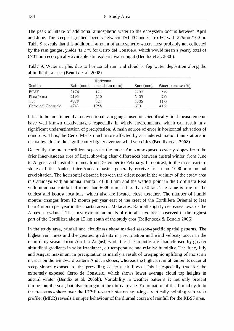
134 5 Study Area

The peak of intake of additional atmospheric water to the ecosystem occurs between April and June. The steepest gradient occurs between TS1 FC and Cerro FC with 275mm/100 m. Table 9 reveals that this additional amount of atmospheric water, most probably not collected by the rain gauges, yields 41.2 % for Cerro del Consuelo, which would mean a yearly total of 6701 mm ecologically available atmospheric water input (Bendix et al. 2008).

Table 9: Water surplus due to horizontal rain and cloud or fog water deposition along the altitudinal transect (Bendix et al. 2008)

It has to be mentioned that conventional rain gauges used in scientifically field measurements have well known disadvantages, especially in windy environments, which can result in a significant underestimation of precipitation. A main source of error is horizontal advection of raindrops. Thus, the Cerro MS is much more affected by an underestimation than stations in the valley, due to the significantly higher average wind velocities (Bendix et al. 2008).

Generally, the main cordillera separates the moist Amazon-exposed easterly slopes from the drier inner-Andean area of Loja, showing clear differences between austral winter, from June to August, and austral summer, from December to February. In contrast, to the moist eastern slopes of the Andes, inter-Andean basins generally receive less than 1000 mm annual precipitation. The horizontal distance between the driest point in the vicinity of the study area in Catamayo with an annual rainfall of 383 mm and the wettest point in the Cordillera Real with an annual rainfall of more than 6000 mm, is less than 30 km. The same is true for the coldest and hottest locations, which also are located close together. The number of humid months changes from 12 month per year east of the crest of the Cordillera Oriental to less than 4 month per year in the coastal area of Malacatos. Rainfall slightly decreases towards the Amazon lowlands. The most extreme amounts of rainfall have been observed in the highest part of the Cordillera about 15 km south of the study area (Rollenbeck & Bendix 2006).

In the study area, rainfall and cloudiness show marked season-specific spatial patterns. The highest rain rates and the greatest gradients in precipitation and wind velocity occur in the main rainy season from April to August, while the drier months are characterised by greater altitudinal gradients in solar irradiance, air temperature and relative humidity. The June, July and August maximum in precipitation is mainly a result of orographic uplifting of moist air masses on the windward eastern Andean slopes, whereas the highest rainfall amounts occur at steep slopes exposed to the prevailing easterly air flows. This is especially true for the extremely exposed Cerro de Consuelo, which shows lower average cloud top heights in austral winter (Bendix et al. 2006b). Variability in weather patterns is not only present throughout the year, but also throughout the diurnal cycle. Examination of the diurnal cycle in the free atmosphere over the ECSF research station by using a vertically pointing rain radar profiler (MRR) reveals a unique behaviour of the diurnal course of rainfall for the RBSF area.

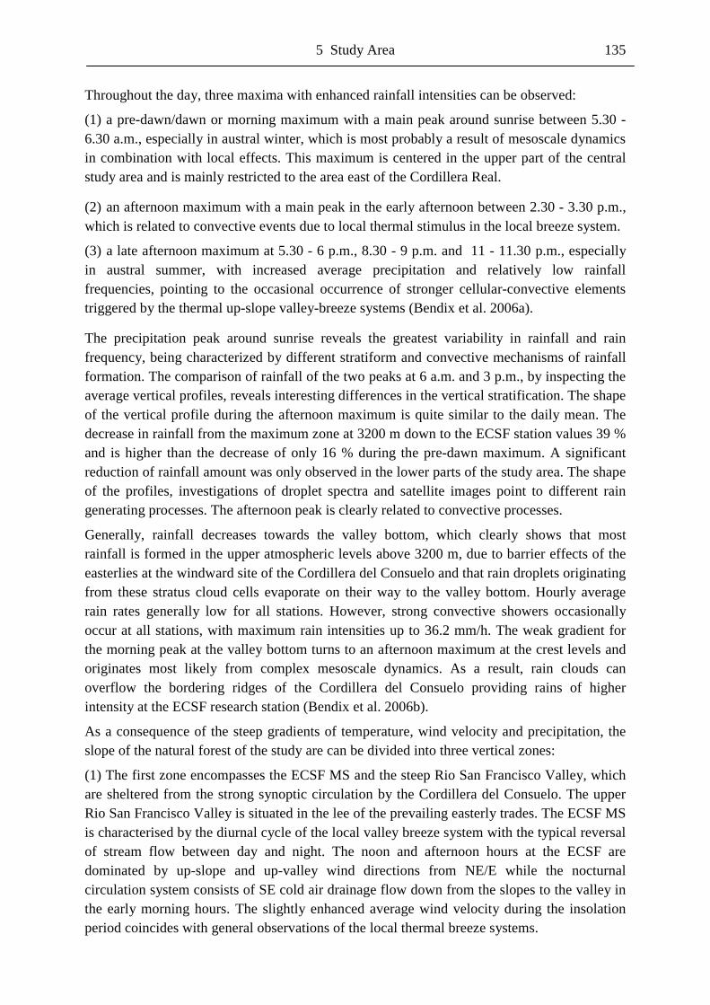
5 Study Area 135

Throughout the day, three maxima with enhanced rainfall intensities can be observed:

(1) a pre-dawn/dawn or morning maximum with a main peak around sunrise between 5.30 -6.30 a.m., especially in austral winter, which is most probably a result of mesoscale dynamics in combination with local effects. This maximum is centered in the upper part of the central study area and is mainly restricted to the area east of the Cordillera Real.

(2) an afternoon maximum with a main peak in the early afternoon between 2.30 - 3.30 p.m., which is related to convective events due to local thermal stimulus in the local breeze system.

(3) a late afternoon maximum at 5.30 - 6 p.m., 8.30 - 9 p.m. and 11 - 11.30 p.m., especially in austral summer, with increased average precipitation and relatively low rainfall frequencies, pointing to the occasional occurrence of stronger cellular-convective elements triggered by the thermal up-slope valley-breeze systems (Bendix et al. 2006a).

The precipitation peak around sunrise reveals the greatest variability in rainfall and rain frequency, being characterized by different stratiform and convective mechanisms of rainfall formation. The comparison of rainfall of the two peaks at 6 a.m. and 3 p.m., by inspecting the average vertical profiles, reveals interesting differences in the vertical stratification. The shape of the vertical profile during the afternoon maximum is quite similar to the daily mean. The decrease in rainfall from the maximum zone at 3200 m down to the ECSF station values 39 % and is higher than the decrease of only 16 % during the pre-dawn maximum. A significant reduction of rainfall amount was only observed in the lower parts of the study area. The shape of the profiles, investigations of droplet spectra and satellite images point to different rain generating processes. The afternoon peak is clearly related to convective processes.

Generally, rainfall decreases towards the valley bottom, which clearly shows that most rainfall is formed in the upper atmospheric levels above 3200 m, due to barrier effects of the easterlies at the windward site of the Cordillera del Consuelo and that rain droplets originating from these stratus cloud cells evaporate on their way to the valley bottom. Hourly average rain rates generally low for all stations. However, strong convective showers occasionally occur at all stations, with maximum rain intensities up to 36.2 mm/h. The weak gradient for the morning peak at the valley bottom turns to an afternoon maximum at the crest levels and originates most likely from complex mesoscale dynamics. As a result, rain clouds can overflow the bordering ridges of the Cordillera del Consuelo providing rains of higher intensity at the ECSF research station (Bendix et al. 2006b).

As a consequence of the steep gradients of temperature, wind velocity and precipitation, the slope of the natural forest of the study are can be divided into three vertical zones:

(1) The first zone encompasses the ECSF MS and the steep Rio San Francisco Valley, which are sheltered from the strong synoptic circulation by the Cordillera del Consuelo. The upper Rio San Francisco Valley is situated in the lee of the prevailing easterly trades. The ECSF MS is characterised by the diurnal cycle of the local valley breeze system with the typical reversal of stream flow between day and night. The noon and afternoon hours at the ECSF are dominated by up-slope and up-valley wind directions from NE/E while the nocturnal circulation system consists of SE cold air drainage flow down from the slopes to the valley in the early morning hours. The slightly enhanced average wind velocity during the insolation period coincides with general observations of the local thermal breeze systems.

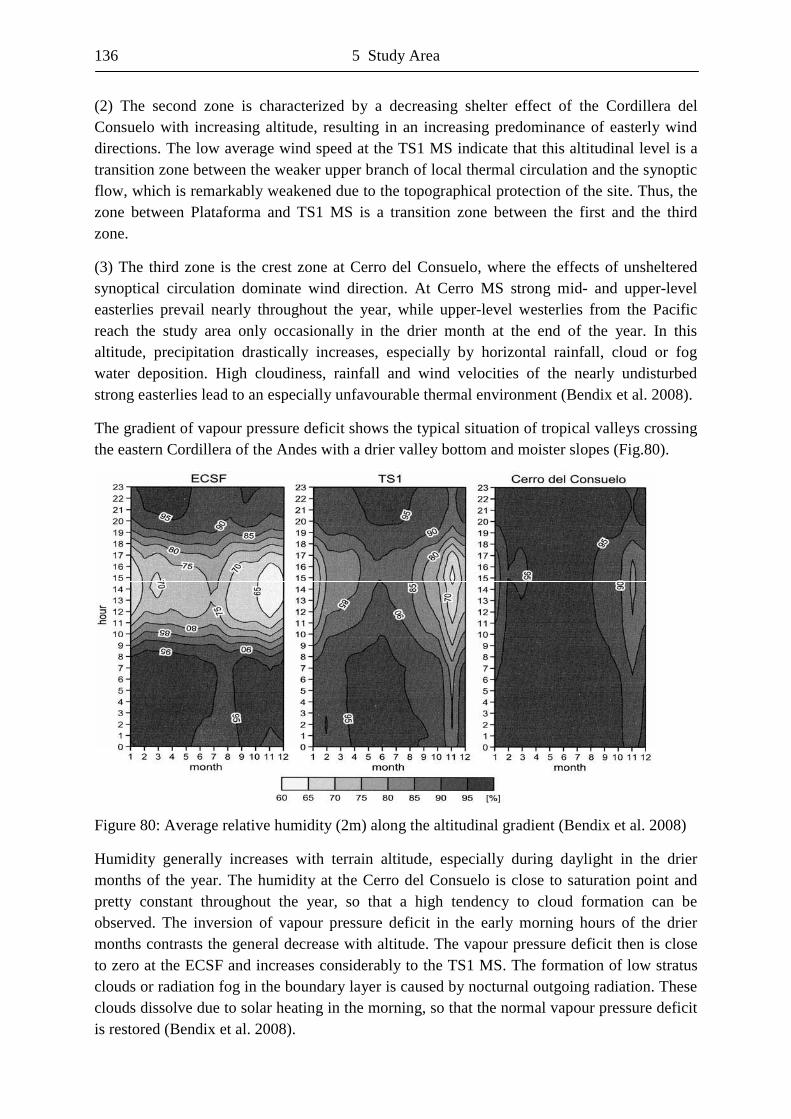
136 5 Study Area

(2) The second zone is characterized by a decreasing shelter effect of the Cordillera del Consuelo with increasing altitude, resulting in an increasing predominance of easterly wind directions. The low average wind speed at the TS1 MS indicate that this altitudinal level is a transition zone between the weaker upper branch of local thermal circulation and the synoptic flow, which is remarkably weakened due to the topographical protection of the site. Thus, the zone between Plataforma and TS1 MS is a transition zone between the first and the third zone.

(3) The third zone is the crest zone at Cerro del Consuelo, where the effects of unsheltered synoptical circulation dominate wind direction. At Cerro MS strong mid- and upper-level easterlies prevail nearly throughout the year, while upper-level westerlies from the Pacific reach the study area only occasionally in the drier month at the end of the year. In this altitude, precipitation drastically increases, especially by horizontal rainfall, cloud or fog water deposition. High cloudiness, rainfall and wind velocities of the nearly undisturbed strong easterlies lead to an especially unfavourable thermal environment (Bendix et al. 2008).

The gradient of vapour pressure deficit shows the typical situation of tropical valleys crossing the eastern Cordillera of the Andes with a drier valley bottom and moister slopes (Fig.80).

Figure 80: Average relative humidity (2m) along the altitudinal gradient (Bendix et al. 2008)

Humidity generally increases with terrain altitude, especially during daylight in the drier months of the year. The humidity at the Cerro del Consuelo is close to saturation point and pretty constant throughout the year, so that a high tendency to cloud formation can be observed. The inversion of vapour pressure deficit in the early morning hours of the drier months contrasts the general decrease with altitude. The vapour pressure deficit then is close to zero at the ECSF and increases considerably to the TS1 MS. The formation of low stratus clouds or radiation fog in the boundary layer is caused by nocturnal outgoing radiation. These clouds dissolve due to solar heating in the morning, so that the normal vapour pressure deficit is restored (Bendix et al. 2008).

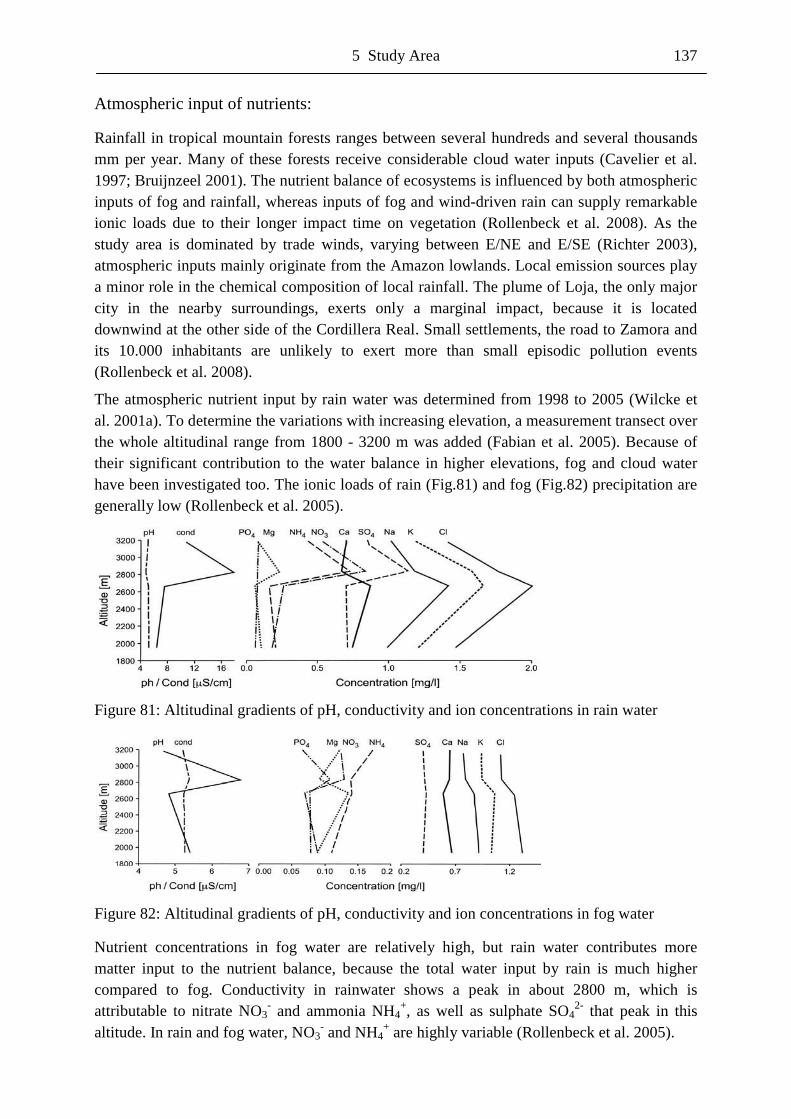
5 Study Area 137

Atmospheric input of nutrients:

Rainfall in tropical mountain forests ranges between several hundreds and several thousands mm per year. Many of these forests receive considerable cloud water inputs (Cavelier et al. 1997; Bruijnzeel 2001). The nutrient balance of ecosystems is influenced by both atmospheric inputs of fog and rainfall, whereas inputs of fog and wind-driven rain can supply remarkable ionic loads due to their longer impact time on vegetation (Rollenbeck et al. 2008). As the study area is dominated by trade winds, varying between E/NE and E/SE (Richter 2003), atmospheric inputs mainly originate from the Amazon lowlands. Local emission sources play a minor role in the chemical composition of local rainfall. The plume of Loja, the only major city in the nearby surroundings, exerts only a marginal impact, because it is located downwind at the other side of the Cordillera Real. Small settlements, the road to Zamora and its 10.000 inhabitants are unlikely to exert more than small episodic pollution events (Rollenbeck et al. 2008).

The atmospheric nutrient input by rain water was determined from 1998 to 2005 (Wilcke et al. 2001a). To determine the variations with increasing elevation, a measurement transect over the whole altitudinal range from 1800 - 3200 m was added (Fabian et al. 2005). Because of their significant contribution to the water balance in higher elevations, fog and cloud water have been investigated too. The ionic loads of rain (Fig.81) and fog (Fig.82) precipitation are generally low (Rollenbeck et al. 2005).

Figure 81: Altitudinal gradients of pH, conductivity and ion concentrations in rain water

Figure 82: Altitudinal gradients of pH, conductivity and ion concentrations in fog water

Nutrient concentrations in fog water are relatively high, but rain water contributes more matter input to the nutrient balance, because the total water input by rain is much higher compared to fog. Conductivity in rainwater shows a peak in about 2800 m, which is attributable to nitrate NO3

- and ammonia NH4+, as well as sulphate SO4

2- that peak in this altitude. In rain and fog water, NO3

- and NH4+ are highly variable (Rollenbeck et al. 2005).

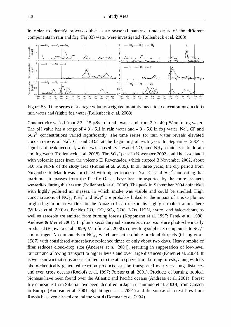
138 5 Study Area

In order to identify processes that cause seasonal patterns, time series of the different components in rain and fog (Fig.83) water were investigated (Rollenbeck et al. 2008).

Figure 83: Time series of average volume-weighted monthly mean ion concentrations in (left) rain water and (right) fog water (Rollenbeck et al. 2008)

Conductivity varied from 2.3 - 15 µS/cm in rain water and from 2.0 - 40 µS/cm in fog water. The pH value has a range of 4.8 - 6.1 in rain water and 4.8 - 5.8 in fog water. Na+, Cl- and SO4

2- concentrations varied significantly. The time series for rain water reveals elevated concentrations of Na+, Cl- and SO4

2- at the beginning of each year. In September 2004 a significant peak occurred, which was caused by elevated NO3

- and NH4+ contents in both rain

and fog water (Rollenbeck et al. 2008). The SO42- peak in November 2002 could be associated

with volcanic gases from the volcano El Reventador, which erupted 3 November 2002, about 500 km N/NE of the study area (Fabian et al. 2005). In all three years, the dry period from November to March was correlated with higher inputs of Na+, Cl- and SO4

2-, indicating that maritime air masses from the Pacific Ocean have been transported by the more frequent westerlies during this season (Rollenbeck et al. 2008). The peak in September 2004 coincided with highly polluted air masses, in which smoke was visible and could be smelled. High concentrations of NO3

-, NH4+ and SO4

2- are probably linked to the impact of smoke plumes originating from forest fires in the Amazon basin due to its highly turbulent atmosphere (Wilcke et al. 2001a). Besides CO2, CO, SO2, COS, NOx, HCN, hydro- and halocarbons, as well as aerosols are emitted from burning forests (Koppmann et al. 1997; Ferek et al. 1998; Andreae & Merlet 2001). In plume secondary substances such as ozone are photo-chemically produced (Fujiwara et al. 1999; Marufu et al. 2000), converting sulphur S compounds to SO4

2- and nitrogen N compounds to NO3

-, which are both soluble in cloud droplets (Chang et al. 1987) with considered atmospheric residence times of only about two days. Heavy smoke of fires reduces cloud-drop size (Andreae et al. 2004), resulting in suppression of low-level rainout and allowing transport to higher levels and over large distances (Koren et al. 2004). It is well-known that substances emitted into the atmosphere from burning forests, along with its photo-chemically generated reaction products, can be transported over very long distances and even cross oceans (Roelofs et al. 1997; Forster et al. 2001). Products of burning tropical biomass have been found over the Atlantic and Pacific oceans (Andreae et al. 2001). Forest fire emissions from Siberia have been identified in Japan (Tanimoto et al. 2000), from Canada in Europe (Andreae et al. 2001, Spichtinger et al. 2001) and the smoke of forest fires from Russia has even circled around the world (Damoah et al. 2004).

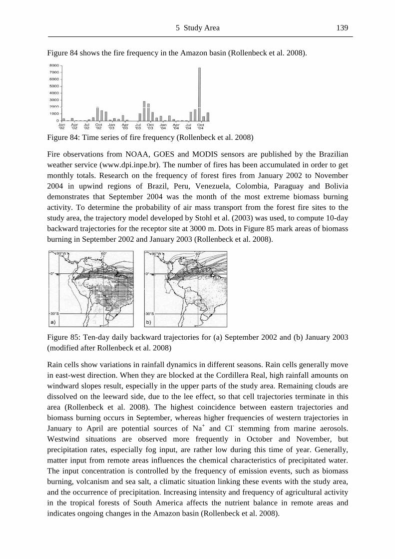
5 Study Area 139

Figure 84 shows the fire frequency in the Amazon basin (Rollenbeck et al. 2008).

Figure 84: Time series of fire frequency (Rollenbeck et al. 2008)

Fire observations from NOAA, GOES and MODIS sensors are published by the Brazilian weather service (www.dpi.inpe.br). The number of fires has been accumulated in order to get monthly totals. Research on the frequency of forest fires from January 2002 to November 2004 in upwind regions of Brazil, Peru, Venezuela, Colombia, Paraguay and Bolivia demonstrates that September 2004 was the month of the most extreme biomass burning activity. To determine the probability of air mass transport from the forest fire sites to the study area, the trajectory model developed by Stohl et al. (2003) was used, to compute 10-day backward trajectories for the receptor site at 3000 m. Dots in Figure 85 mark areas of biomass burning in September 2002 and January 2003 (Rollenbeck et al. 2008).

Figure 85: Ten-day daily backward trajectories for (a) September 2002 and (b) January 2003 (modified after Rollenbeck et al. 2008)

Rain cells show variations in rainfall dynamics in different seasons. Rain cells generally move in east-west direction. When they are blocked at the Cordillera Real, high rainfall amounts on windward slopes result, especially in the upper parts of the study area. Remaining clouds are dissolved on the leeward side, due to the lee effect, so that cell trajectories terminate in this area (Rollenbeck et al. 2008). The highest coincidence between eastern trajectories and biomass burning occurs in September, whereas higher frequencies of western trajectories in January to April are potential sources of Na+ and Cl- stemming from marine aerosols. Westwind situations are observed more frequently in October and November, but precipitation rates, especially fog input, are rather low during this time of year. Generally, matter input from remote areas influences the chemical characteristics of precipitated water. The input concentration is controlled by the frequency of emission events, such as biomass burning, volcanism and sea salt, a climatic situation linking these events with the study area, and the occurrence of precipitation. Increasing intensity and frequency of agricultural activity in the tropical forests of South America affects the nutrient balance in remote areas and indicates ongoing changes in the Amazon basin (Rollenbeck et al. 2008).

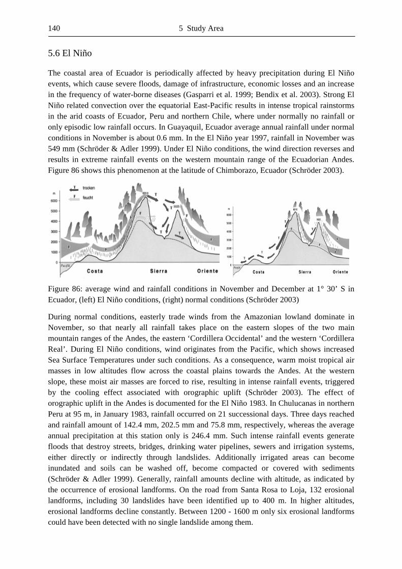
140 5 Study Area

5.6 El Niño

The coastal area of Ecuador is periodically affected by heavy precipitation during El Niño events, which cause severe floods, damage of infrastructure, economic losses and an increase in the frequency of water-borne diseases (Gasparri et al. 1999; Bendix et al. 2003). Strong El Niño related convection over the equatorial East-Pacific results in intense tropical rainstorms in the arid coasts of Ecuador, Peru and northern Chile, where under normally no rainfall or only episodic low rainfall occurs. In Guayaquil, Ecuador average annual rainfall under normal conditions in November is about 0.6 mm. In the El Niño year 1997, rainfall in November was 549 mm (Schröder & Adler 1999). Under El Niño conditions, the wind direction reverses and results in extreme rainfall events on the western mountain range of the Ecuadorian Andes. Figure 86 shows this phenomenon at the latitude of Chimborazo, Ecuador (Schröder 2003).

Figure 86: average wind and rainfall conditions in November and December at 1° 30’ S in Ecuador, (left) El Niño conditions, (right) normal conditions (Schröder 2003)

During normal conditions, easterly trade winds from the Amazonian lowland dominate in November, so that nearly all rainfall takes place on the eastern slopes of the two main mountain ranges of the Andes, the eastern ‘Cordillera Occidental’ and the western ‘Cordillera Real’. During El Niño conditions, wind originates from the Pacific, which shows increased Sea Surface Temperatures under such conditions. As a consequence, warm moist tropical air masses in low altitudes flow across the coastal plains towards the Andes. At the western slope, these moist air masses are forced to rise, resulting in intense rainfall events, triggered by the cooling effect associated with orographic uplift (Schröder 2003). The effect of orographic uplift in the Andes is documented for the El Niño 1983. In Chulucanas in northern Peru at 95 m, in January 1983, rainfall occurred on 21 successional days. Three days reached and rainfall amount of 142.4 mm, 202.5 mm and 75.8 mm, respectively, whereas the average annual precipitation at this station only is 246.4 mm. Such intense rainfall events generate floods that destroy streets, bridges, drinking water pipelines, sewers and irrigation systems, either directly or indirectly through landslides. Additionally irrigated areas can become inundated and soils can be washed off, become compacted or covered with sediments (Schröder & Adler 1999). Generally, rainfall amounts decline with altitude, as indicated by the occurrence of erosional landforms. On the road from Santa Rosa to Loja, 132 erosional landforms, including 30 landslides have been identified up to 400 m. In higher altitudes, erosional landforms decline constantly. Between 1200 - 1600 m only six erosional landforms could have been detected with no single landslide among them.

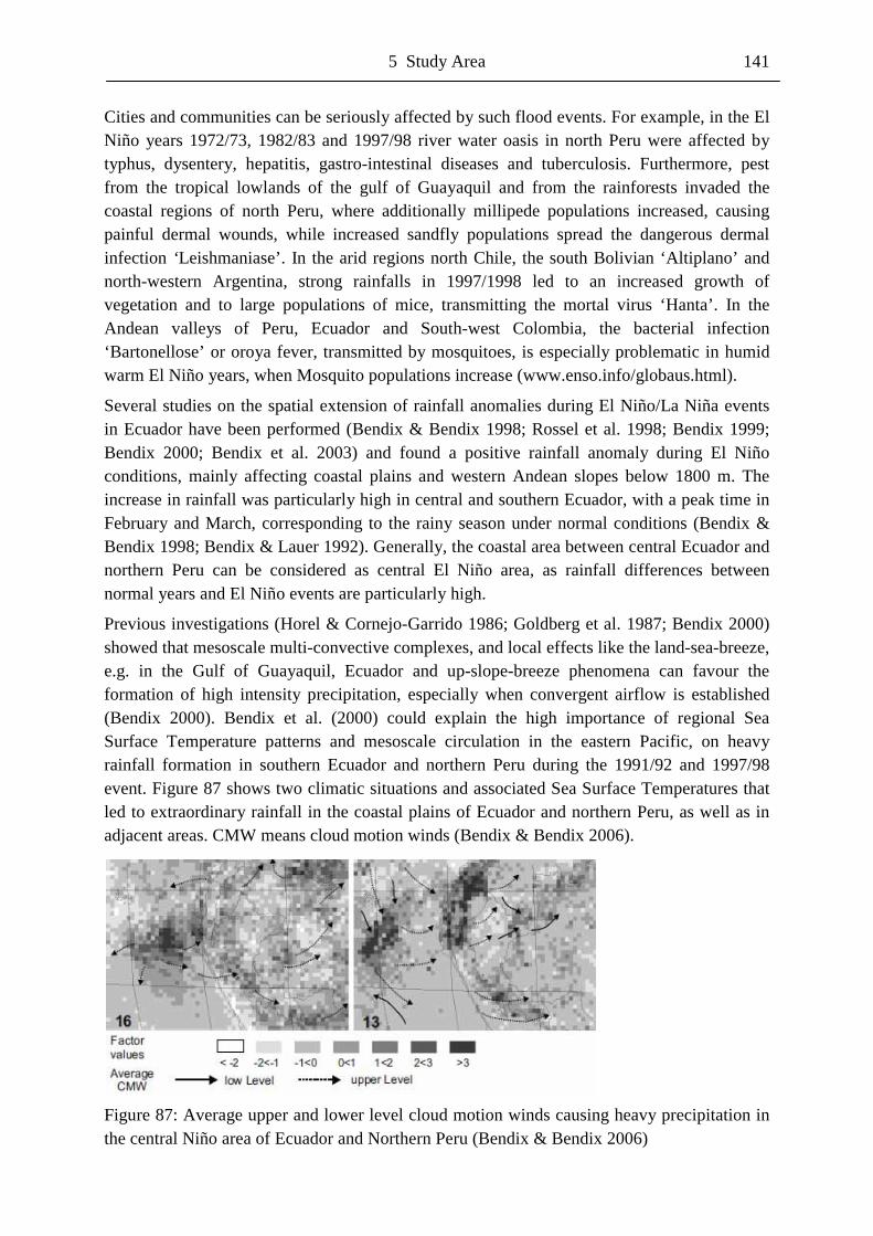
5 Study Area 141

Cities and communities can be seriously affected by such flood events. For example, in the El Niño years 1972/73, 1982/83 and 1997/98 river water oasis in north Peru were affected by typhus, dysentery, hepatitis, gastro-intestinal diseases and tuberculosis. Furthermore, pest from the tropical lowlands of the gulf of Guayaquil and from the rainforests invaded the coastal regions of north Peru, where additionally millipede populations increased, causing painful dermal wounds, while increased sandfly populations spread the dangerous dermal infection ‘Leishmaniase’. In the arid regions north Chile, the south Bolivian ‘Altiplano’ and north-western Argentina, strong rainfalls in 1997/1998 led to an increased growth of vegetation and to large populations of mice, transmitting the mortal virus ‘Hanta’. In the Andean valleys of Peru, Ecuador and South-west Colombia, the bacterial infection ‘Bartonellose’ or oroya fever, transmitted by mosquitoes, is especially problematic in humid warm El Niño years, when Mosquito populations increase (www.enso.info/globaus.html).

Several studies on the spatial extension of rainfall anomalies during El Niño/La Niña events in Ecuador have been performed (Bendix & Bendix 1998; Rossel et al. 1998; Bendix 1999; Bendix 2000; Bendix et al. 2003) and found a positive rainfall anomaly during El Niño conditions, mainly affecting coastal plains and western Andean slopes below 1800 m. The increase in rainfall was particularly high in central and southern Ecuador, with a peak time in February and March, corresponding to the rainy season under normal conditions (Bendix & Bendix 1998; Bendix & Lauer 1992). Generally, the coastal area between central Ecuador and northern Peru can be considered as central El Niño area, as rainfall differences between normal years and El Niño events are particularly high.

Previous investigations (Horel & Cornejo-Garrido 1986; Goldberg et al. 1987; Bendix 2000) showed that mesoscale multi-convective complexes, and local effects like the land-sea-breeze, e.g. in the Gulf of Guayaquil, Ecuador and up-slope-breeze phenomena can favour the formation of high intensity precipitation, especially when convergent airflow is established (Bendix 2000). Bendix et al. (2000) could explain the high importance of regional Sea Surface Temperature patterns and mesoscale circulation in the eastern Pacific, on heavy rainfall formation in southern Ecuador and northern Peru during the 1991/92 and 1997/98 event. Figure 87 shows two climatic situations and associated Sea Surface Temperatures that led to extraordinary rainfall in the coastal plains of Ecuador and northern Peru, as well as in adjacent areas. CMW means cloud motion winds (Bendix & Bendix 2006).

Figure 87: Average upper and lower level cloud motion winds causing heavy precipitation in the central Niño area of Ecuador and Northern Peru (Bendix & Bendix 2006)

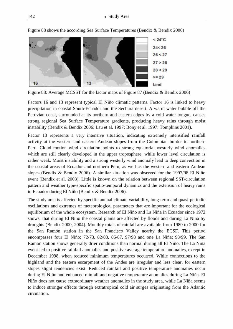
142 5 Study Area

Figure 88 shows the according Sea Surface Temperatures (Bendix & Bendix 2006)

Figure 88: Average MCSST for the factor maps of Figure 87 (Bendix & Bendix 2006)

Factors 16 and 13 represent typical El Niño climatic patterns. Factor 16 is linked to heavy precipitation in coastal South-Ecuador and the Sechura desert. A warm water bubble off the Peruvian coast, surrounded at its northern and eastern edges by a cold water tongue, causes strong regional Sea Surface Temperature gradients, producing heavy rains through moist instability (Bendix & Bendix 2006; Lau et al. 1997; Bony et al. 1997; Tompkins 2001).

Factor 13 represents a very intensive situation, indicating extremely intensified rainfall activity at the western and eastern Andean slopes from the Colombian border to northern Peru. Cloud motion wind circulation points to strong equatorial westerly wind anomalies which are still clearly developed in the upper troposphere, while lower level circulation is rather weak. Moist instability and a strong westerly wind anomaly lead to deep convection in the coastal areas of Ecuador and northern Peru, as well as the western and eastern Andean slopes (Bendix & Bendix 2006). A similar situation was observed for the 1997/98 El Niño event (Bendix et al. 2003). Little is known on the relation between regional SST/circulation pattern and weather type-specific spatio-temporal dynamics and the extension of heavy rains in Ecuador during El Niño (Bendix & Bendix 2006).

The study area is affected by specific annual climate variability, long-term and quasi-periodic oscillations and extremes of meteorological parameters that are important for the ecological equilibrium of the whole ecosystem. Research of El Niño and La Niña in Ecuador since 1972 shows, that during El Niño the coastal plains are affected by floods and during La Niña by droughts (Bendix 2000, 2004). Monthly totals of rainfall are available from 1980 to 2000 for the San Ramón station in the San Francisco Valley nearby the ECSF. This period encompasses four El Niño: 72/73, 82/83, 86/87, 97/98 and one La Niña: 98/99. The San Ramon station shows generally drier conditions than normal during all El Niño. The La Niña event led to positive rainfall anomalies and positive average temperature anomalies, except in December 1998, when reduced minimum temperatures occurred. While connections to the highland and the eastern escarpment of the Andes are irregular and less clear, for eastern slopes slight tendencies exist. Reduced rainfall and positive temperature anomalies occur during El Niño and enhanced rainfall and negative temperature anomalies during La Niña. El Niño does not cause extraordinary weather anomalies in the study area, while La Niña seems to induce stronger effects through extratropical cold air surges originating from the Atlantic circulation.

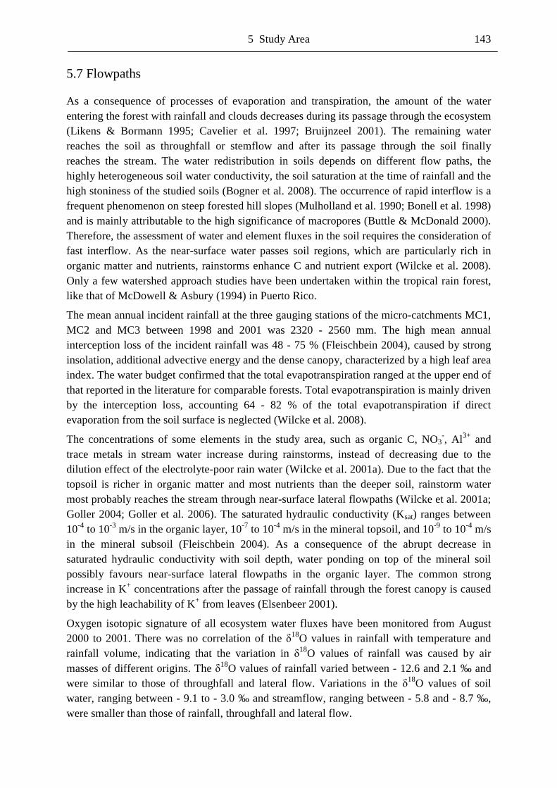
5 Study Area 143

5.7 Flowpaths

As a consequence of processes of evaporation and transpiration, the amount of the water entering the forest with rainfall and clouds decreases during its passage through the ecosystem (Likens & Bormann 1995; Cavelier et al. 1997; Bruijnzeel 2001). The remaining water reaches the soil as throughfall or stemflow and after its passage through the soil finally reaches the stream. The water redistribution in soils depends on different flow paths, the highly heterogeneous soil water conductivity, the soil saturation at the time of rainfall and the high stoniness of the studied soils (Bogner et al. 2008). The occurrence of rapid interflow is a frequent phenomenon on steep forested hill slopes (Mulholland et al. 1990; Bonell et al. 1998) and is mainly attributable to the high significance of macropores (Buttle & McDonald 2000). Therefore, the assessment of water and element fluxes in the soil requires the consideration of fast interflow. As the near-surface water passes soil regions, which are particularly rich in organic matter and nutrients, rainstorms enhance C and nutrient export (Wilcke et al. 2008). Only a few watershed approach studies have been undertaken within the tropical rain forest, like that of McDowell & Asbury (1994) in Puerto Rico.

The mean annual incident rainfall at the three gauging stations of the micro-catchments MC1, MC2 and MC3 between 1998 and 2001 was 2320 - 2560 mm. The high mean annual interception loss of the incident rainfall was 48 - 75 % (Fleischbein 2004), caused by strong insolation, additional advective energy and the dense canopy, characterized by a high leaf area index. The water budget confirmed that the total evapotranspiration ranged at the upper end of that reported in the literature for comparable forests. Total evapotranspiration is mainly driven by the interception loss, accounting 64 - 82 % of the total evapotranspiration if direct evaporation from the soil surface is neglected (Wilcke et al. 2008).

The concentrations of some elements in the study area, such as organic C, NO3-, Al3+ and

trace metals in stream water increase during rainstorms, instead of decreasing due to the dilution effect of the electrolyte-poor rain water (Wilcke et al. 2001a). Due to the fact that the topsoil is richer in organic matter and most nutrients than the deeper soil, rainstorm water most probably reaches the stream through near-surface lateral flowpaths (Wilcke et al. 2001a; Goller 2004; Goller et al. 2006). The saturated hydraulic conductivity (Ksat) ranges between 10-4 to 10-3 m/s in the organic layer, 10-7 to 10-4 m/s in the mineral topsoil, and 10-9 to 10-4 m/s in the mineral subsoil (Fleischbein 2004). As a consequence of the abrupt decrease in saturated hydraulic conductivity with soil depth, water ponding on top of the mineral soil possibly favours near-surface lateral flowpaths in the organic layer. The common strong increase in K+ concentrations after the passage of rainfall through the forest canopy is caused by the high leachability of K+ from leaves (Elsenbeer 2001).

Oxygen isotopic signature of all ecosystem water fluxes have been monitored from August 2000 to 2001. There was no correlation of the �18O values in rainfall with temperature and rainfall volume, indicating that the variation in �18O values of rainfall was caused by air masses of different origins. The �18O values of rainfall varied between - 12.6 and 2.1 ‰ and were similar to those of throughfall and lateral flow. Variations in the �18O values of soil water, ranging between - 9.1 to - 3.0 ‰ and streamflow, ranging between - 5.8 and - 8.7 ‰, were smaller than those of rainfall, throughfall and lateral flow.

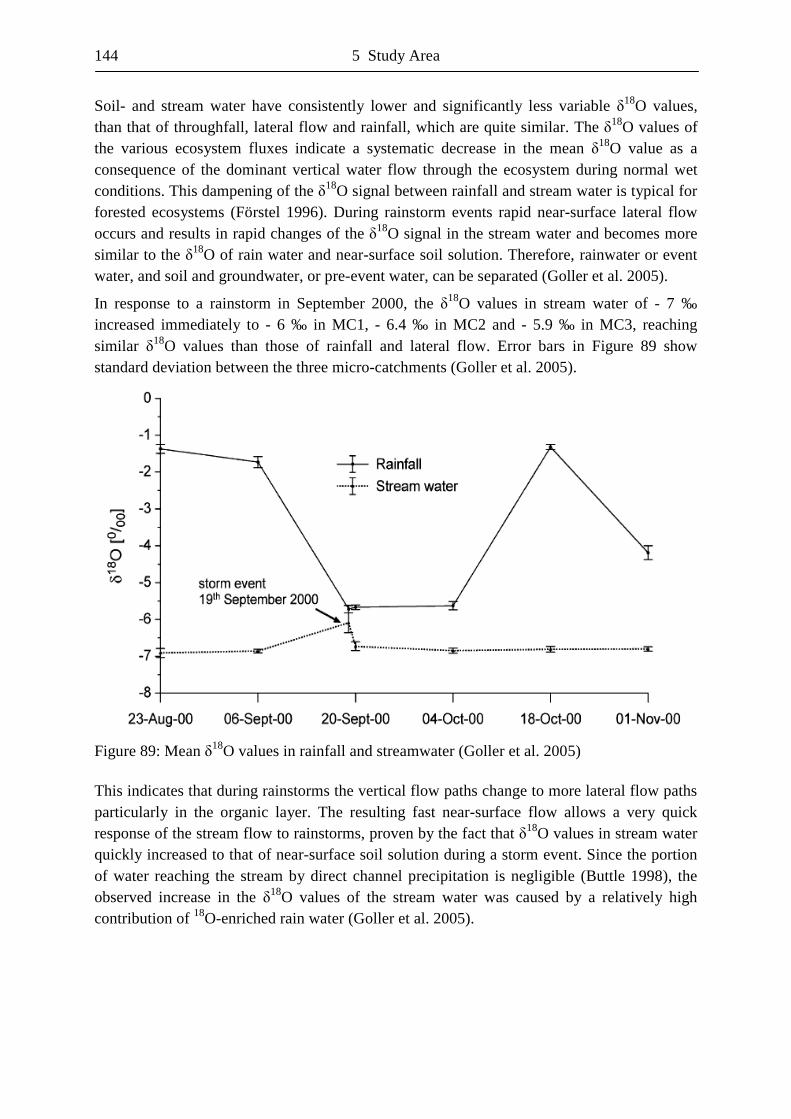
144 5 Study Area

Soil- and stream water have consistently lower and significantly less variable �18O values, than that of throughfall, lateral flow and rainfall, which are quite similar. The �18O values of the various ecosystem fluxes indicate a systematic decrease in the mean �18O value as a consequence of the dominant vertical water flow through the ecosystem during normal wet conditions. This dampening of the �18O signal between rainfall and stream water is typical for forested ecosystems (Förstel 1996). During rainstorm events rapid near-surface lateral flow occurs and results in rapid changes of the �18O signal in the stream water and becomes more similar to the �18O of rain water and near-surface soil solution. Therefore, rainwater or event water, and soil and groundwater, or pre-event water, can be separated (Goller et al. 2005).

In response to a rainstorm in September 2000, the �18O values in stream water of - 7 ‰ increased immediately to - 6 ‰ in MC1, - 6.4 ‰ in MC2 and - 5.9 ‰ in MC3, reaching similar �18O values than those of rainfall and lateral flow. Error bars in Figure 89 show standard deviation between the three micro-catchments (Goller et al. 2005).

Figure 89: Mean �18O values in rainfall and streamwater (Goller et al. 2005) This indicates that during rainstorms the vertical flow paths change to more lateral flow paths particularly in the organic layer. The resulting fast near-surface flow allows a very quick response of the stream flow to rainstorms, proven by the fact that �18O values in stream water quickly increased to that of near-surface soil solution during a storm event. Since the portion of water reaching the stream by direct channel precipitation is negligible (Buttle 1998), the observed increase in the �18O values of the stream water was caused by a relatively high contribution of 18O-enriched rain water (Goller et al. 2005).

5 Study Area 145

The assumption was confirmed by the course of soil water content, showing a higher water content of the organic layer, compared to the upper mineral soil (Fig.90), during the studied rainstorm event (Goller et al. 2005).

Figure 90: Course of soil water content during a rainstorm event (Goller et al. 2005)

Soil water content in transect MC2.1 started increasing continuously 6 days before the event, on 13.09, after a period of drier conditions. The hydrograph of the rainstorm event on 19.09 shows three smaller rain events prior to the actual rainstorm event, resulting in a high pre-saturation of the soils. The rise of the water content was considerably higher in the O horizon compared with the A horizon, indicating the occurrence and domination of lateral ‘organic horizon flow’ (Kendall et al. 1999) in the uppermost part of the soil during the rainstorm event (Goller et al. 2005). This interpretation is further confirmed by considerably higher saturated hydraulic conductivity in the organic layer with 4.5 * 10-4 m/s, compared with the upper mineral soil with a Ksat of 1.8 *10-6 m/s and the lower mineral soil with a Ksat of 1.4 * 10-7 m/s in MC2 (Fleischbein 2004). A decrease of soil hydrologic conductivity with depth is commonly considered as prerequisite for the occurrence of interflow (Caspar 2002).

Results from a two-component hydrograph separation of the rainstorm on 19.09 revealed a high contribution of event water to stormflow runoff in MC1 and MC3, with 81 and 78 %, respectively. A distinctly lower event water contribution of 44 % was reported for the MC2, indicating that the significance of stormflow generating processes may vary even in catchments with comparable climatic and edaphic conditions (Goller et al. 2005). This result partly contrasts the findings of numerous small catchment studies, which reported a dominance of pre-event water in stormflow runoff and supports fewer studies that found the event water component to be predominant (Bonell et al. 1998; Schellekens et al. 2004). Bonell et al. (1998) emphasized that rainfall intensity is a major factor for the response of small water catchments in high-rainfall areas. According to Sklash et al. (1986), the displacement of pre-event water can occur due to groundwater ridging, particularly in pre-saturated lower parts of the slope (Ward 1984). Old water contribution by groundwater ridging in MC2 was promoted by lower rainfall intensity in MC2 during the rainstorm event and the topographic position in a depression (Goller et al. 2005).

146 5 Study Area

5.8 Water Chemistry

The major purpose of forest ecosystem research in the past decades was to assess the human impact on cycles of C, N, P, and S and to understand element sources and sinks, as well as controls of their mobility (Likens & Bormann 1995; Matson et al. 1999; Matzner 2004). The biogeochemical cycles of N, P, and S are complex, as different chemical species are involved, which additionally are influenced by fertilizers and the deposition of NOx and SO2, which are released during combustion of fossil fuels (Wilcke et al. 2008b).

Low rainfall intensities and associated slow wash-off processes lead to an incomplete removal of dry deposition from the canopy. The resulting long contact time of rain water with the canopy surface leads to high ion concentrations. In contrast, high rainfall intensities lead to a complete depletion of the leachable ion pools of NH4

+, NO3- and PO4

3- of the canopy (Lovett & Schaefer 1992). The main ‘reactor’ compartments of forests are the canopy and the soil. The canopy of tropical forests can be a sink for plant nutrients, due to uptake processes enforced by the leaves (Bentley 1987; Schrumpf 2004), but nutrients can also be leached from the canopy, which might be a particularly true for organic species (Lilienfein & Wilcke 2004). Canopy leaching has proved to be the major source of dissolved PO4

3- (Parker 1983) and dissolved organic N in throughfall (Qualls et al. 1991). Furthermore, nutrients can be released by the mineralization of dead organic matter accumulated in the canopy (Bentley & Carpenter 1980; Coxson 1990). In temperate forests, the soil organic layer is usually the main source of dissolved organic matter (DOM) including associated N, P and S (Kaiser et al. 2000; Kalbitz et al. 2000; Michalzik et al. 2001). In temperate and tropical forests, the soil organic layer is a sink of inorganic N, P and S due to microbial immobilization (Yavitt & Fahey 1986; Qualls et al. 1991; Alewell et al. 1999) and the conservation by roots and mycorrhizae (Stark & Jordan 1978; Cuevas & Medina 1986). In some tropical forests, inorganic N concentrations in litter leachate are higher than in throughfall, indicating that inorganic N is leached from the organic layer because N release rates by mineralization are higher than the requirement of the vegetation and soil microorganisms (Hafkenscheid 2000; Wilcke et al. 2001; Schrumpf 2004). Dissolved P in forests on acid soils, primarily cycles between the canopy and the organic layer, as a consequence of P fixation in the mineral soils (Sanchez 1976; Sollins et al. 1988; Stevenson & Cole 1999). The microbial release of SO4

2- during mineralization is a major source of soluble S in many soils (Stevenson & Cole 1999).

Important controls of element cycles on the soil and catchment scale are soil pH and the water flow regime. Although an increasing pH promotes the release of DOM (Kalbitz et al. 2000), results from laboratory and field experiments are inconsistent (Michalzik et al. 2001). Contrasting results have also been reported concerning the effect of pH on microbial activity and associated nitrification rates. While some authors conclude that low pH values reduce nitrification, as a consequence of reduced activities of autotroph nitrifiers (Kilham 1990), others did not detect this relationship (Robertsen 1982). The water flux in soils is a major control of the dynamics of inorganic N (Mitchell 2001), DOC and DON (Hagedorn et al. 2000), total P (Frangi & Lugo 1985), DOP and DOS (Kaiser et al. 2000) in forested water catchments, especially after rainstorms. As small water catchments on steep hillslopes in tropical regions show a rapid response of catchment discharge to strongly increasing rainfall intensities and volumes, the influence of water fluxes on element dynamics should also be

5 Study Area 147

prominent there (Mulholland et al. 1990; Schellekens 2000). The increase in DOC concentrations in catchment runoff during high flow has been documented in many studies (Jardine et al. 1990; Brown et al. 1999; Casper 2002). Similar observations were reported for NO3

- by Mitchell (2001) and for PO43- by Frangi & Lugo (1985).

Goller et al. (2005) showed that during rainstorms flow paths of water in the soil switched rapidly from mainly vertical to mainly near-surface lateral flow, where concentrations of organic C and N are highest. Accordingly, Wilcke et al. (2001) reported an increase in DOC concentrations in streams during high flow conditions. Increased DOC and DON concentrations in stream water in response to rainstorms indicate that also DOM export is increased during elevated discharge. One reason might be the flushing of soluble organic compounds accumulated during preceding dry periods from the organic layer into the streams (Kalbitz et al. 2000; Qualls et al. 2002). The significantly higher three-year means of DOC and DON concentrations in stream water during stormflow than under non-storm conditions suggests that the frequently occurring rainstorm events may cause a considerable loss of C and N from the catchments (Goller et al. 2006).

DOM is the major vector for most fluxes of N, P, and S. Although DON, DOP, and DOS concentrations were all correlated with those of DOC, indicating that their biochemical dynamics were linked, differences in the contribution of the organic forms to the total nutrient fluxes imply that the cycles of N, P, and S are partly decoupled, particularly in the soil. The canopy was the largest source of dissolved inorganic N and P, the organic layer of DOC, DON, DOP and DOS, and the mineral soil of dissolved SO4

2-. The forest canopy also released considerable amounts of DOC, DON, DOP and DOS. The organic layer was a sink for dissolved inorganic N, P, and S and the mineral soil for all studied C, N, P and S forms except SO4

2-. The concentrations of NO3- and DON in soil solutions tended to be positively related to

pH. Hydrological conditions controlled N, P and S transport and transformation through the ecosystem. Dissolved inorganic N, P, and S concentrations were increased during dry periods probably because of the dying of microorganisms. In contrast, DON concentrations in soil solutions were reduced during dry periods because of sorption followed by a DON from the organic layer after rewetting. Rainstorms associated with short-time high-intensive rainfall, occurring from time to time at the study site, appeared to be responsible for a considerable increase in C and N and possibly P and S concentrations in catchment runoff. This indicated an elevated export of these elements from the studied forest during periods of stormflow because of fast near-surface lateral water flow (Goller et al. 2006).

Goller et al. (2006) reported increases in dissolved organic carbon (DOC) and N concentrations, as well as decreased pH values during high-flow conditions. The finding that there was no dilution of the N concentrations with increasing electrolyte-poor rainfall suggest that the fast percolating near-surface water after strong rainstorms on already pre-saturated soils carries organic matter and organically bound nutrients to the stream (Goller et al. 2005). However, this was not the case for the base metals, suggesting that the higher leaching during rainstorms of these metals which accumulate in the organic layer and topsoil (Wilcke et al. 2002) was compensated by other sources during baseflow conditions, such as mineral weathering and deep leaching.

148 5 Study Area

5.9 Nutrient Fluxes

In the study area, strong interannual variations of nutrient inputs, due to climatic changes and/or anthropogenic activity, influence the nutrient budget. The quality of ecosystem solutions such as throughfall, litter leachate, and soil solution was considerably variable (Wilcke et al. 2008b), coinciding with variable soil properties and associated numerous different ecological niches at a small scale (Wilcke et al. 2003). Major factors of nutrient fluxes in forest ecosystems are rainfall, litter fall and organic matter turnover. The chemical composition and quantity of rainfall and cloud water changes during its passage through the forest (Parker 1983). Generally nutrient concentrations, except for elements which are released by weathering, are lower in streamwater than in litter leachate (Bruijnzeel et al. 1993; McDowell 1998). The turnover of organic matter in tropical forests is fast for fine litter, intermediate for coarse woody debris and slow for living trees (Clark et al. 2002). Weathered or nutrient-poor soils contain most plant available nutrients (Cuevas & Medina 1986; Grubb 1995; Kauffman et al. 1998). The plant availability of N, P and S in the organic layers depends largely on mineralization rates, while base metals are mainly bound in exchangeable form (Vogt et al. 1986, Proctor 1987).

Deposition and canopy interaction

In mountainous forests in the northern Andes, pH values range from 4.4 to 5.6 (Steinhardt 1979, Veneklaas 1990). The volume-weighted mean pH of rainfall in the study area between the five study years and the three gauging stations MC1, MC2 and MC3 was 5.3 (Wilcke et al. 2003). During the passage through the canopy, pH was buffered to 6.2 in throughfall. pH values were slightly more acid in most years than expected, which might be a consequence of the input of mineral acids, originating from forest fires in the Amazon basin (Fabian et al. 2005), and/or the release of organic acids from the canopy of the Amazon lowland rainforest (Forti & Neal 1992). The volume-weighted mean concentrations of N, P, K, Ca and Mg in incident rainfall were similar or in the lower half of the range of concentrations compared to lower mountain rain forests in Central and South America. Volume-weighted mean concentrations of all nutrients increased in throughfall relative to rainfall and were at the upper end or above the range of concentrations compared with lower mountain rain forests (Hafkenscheid 2000; Wilcke et al. 2008b). Reasons for the enrichment of nutrients in throughfall are evaporation of intercepted water, particulate and gaseous dry deposition, hidden cloud water deposition, which occurs when water droplets evaporate, and canopy processes (Parker 1983). The most important canopy processes are leaching from the plant surfaces, N fixation, decomposition of plant debris in the crown, and insect excretions (Parker 1983; Schaefer & Reiners 1990). The rainfall deposition of N and P in the study area was similar to or above the data range of Hafkenscheid (2000), while the deposition of base metals was consistently at the lower end. Throughfall deposition for all elements was higher than rainfall deposition, with the exception of H+-Protons, which were buffered during the passage through the canopy, resulting in the release of base metals. Dry deposition for all elements had a size similar to that for bulk deposition with incident rainfall, indicating dust and gas inputs into the study area (Wilcke et al. 2008b). The remote location of the study area explains the generally low element concentrations in rainfall, but base metal composition in rainfall varied markedly. The weekly incident rainfall depositions of Ca2+ were highly

5 Study Area 149

variable and closely linked to Mg2+ and K+. In the hydrological years 98/99, 00/01, 01/02 and 02/03, rainfall depositions of Ca2+ were quite similar with 2.4 - 4.4 kg/ha*year, but much lower compared to the hydrological year 99/00, with 16 kg/ha*year. The variation in the annual rainfall deposition rates of Ca2+, Mg2+ and K+ could not be explained by seasonality and also were not related to the dilution effect of rainfall. Investigations in order to explore possible links to long-term climatic cycles, such as El Niño, suggest a 94 - 98 % similarity of weekly Ca2+ deposition rates with changes in the Sea Surface Temperature in the Pacific, indicating that long-term climatic variations influence the atmospheric input of nutrients. In three hydrological years, Ca2+ was leached from the canopy, while Ca2+ was retained by the canopy in the hydrological years 99/00 and 00/01, suggesting a higher Ca2+ uptake by the ecosystem (Wilcke et al. 2008b).

Litterfall and coarse woody debris

The study area produces an average annual biomass of 7.5 - 13.3 t/ha, likewise the tropical lowland forest. The average annual fine litter fall, ranging from 9.1 - 12 t/ha, was at the upper end of the range for various tropical mountain forests globally and is also comparable to that of tropical lowland forests (Vitousek 1984; Bruijnzeel & Proctor 1995; Hafkenscheid 2000). The mass-weighted mean concentrations of all five major nutrients in fine litterfall and element deposition rates differed considerably between transects und were at the upper end or greater than the range of concentrations of other tropical mountain forests (Hafkenscheid 2000). Concentrations of P, Ca2+ and Mg2+ in litterfall were closely related with their respective concentrations in the organic layer, indicating the uptake of these elements by the vegetation. In soils with a higher pH of the organic layer, the uptake is stronger and the nutrient cycling faster. Fine litterfall was the most important flux to the soil for all elements, except for K+ (Wilcke et al. 2001a). The average total coarse woody debris mass of 9.1 t/ha is comparable to the annual litterfall, but highly variable among the studied nine plots. As coarse woody debris is slowly turned over, at a similar rate as the whole organic layer, it contributes little to the nutrient supply via mineralization. More precisely, coarse woody debris contributes less than 1.8 % to the nutrient storage in the aboveground dead biomass. 40 % of the mass of coarse woody debris did not have contact to the soil and no relationship between topographic position, stand properties, mass, C and nutrient storage of coarse woody debris could be observed (Wilcke et al. 2008b)

Organic Matter Turnover

The annual litter is completely turned over within less than 1.5 years and the whole organic layer at the scale of 2 - 3 decades. KOi values represent the mean residence time of organic matter or a single element in the Oi horizon, while KOL values represent the mean residence time of organic matter or a single element in the whole organic layer. The calculated quotient of the storage of mass or nutrient in the Oi horizon and in the whole organic layer, to the annual flux of mass or the same nutrient by litterfall (KOi) is similar to the inverse value of KL used in literature (e.g. Edwards 1982; Heaney & Proctor 1989; Smith et al. 1998). The residence time integrates all scattering processes, such as release of CO2 and other gases, leaching, uptake by plants and animals, but may be biased by retention of element reaching the soil via throughfall and stemflow and by the not considered input of root litter. KOi values of the organic matter mass in the study area range between 0.9 - 1.5 years and are at the upper

150 5 Study Area

end or greater than the range of 0.6 - 1.2 years, reported for other tropical mountain forests (Edwards 1982; Heaney & Proctor 1989; Bruijnzeel et al. 1993). The mean KOL value of the mass is 11 times greater than the KOi value, indicating that the turnover of organic matter in the organic layer is slower than in other tropical mountain forests. The annual nutrient release from coarse woody debris contributed at most 1.5 % of the total plant-available nutrients in the forest soil, possibly being attributable to the thick organic layers (Wilcke et al. 2008b).

Soil solution

The average medians of the volume-weighted mean pH in litter leachates were 4.7 (MC2/1), 5.7 (MC2/2), 5.9 (MC2/3) and 6.0 (MC1). The pH values in throughfall were all higher, with 6.3 (MC2/1), 6.1 (MC2/2), 6.2 (MC2/3) and 6.5 (MC1), indicating that additional acids, such as acidic components of dissolved organic matter (DOM) were leached from the organic layer. In MC3, the pH of the litter leachate reflects the pH of the organic layer. Thus, the organic layer of MC1 and MC3 are better buffered than the more acid MC2. Volume-weighted mean pH values of the organic layers in MC2, ranging from 4.4 - 4.7, were more acid than respective pH values of the organic layers in MC1 and MC3, ranging from 6.2 - 6.3. All average medians of major nutrient concentrations in litter leachate were higher than in two Jamaican upper montane cloud forests, except for P at all study transects and base metals at transects MC 2/1 and MC 2/2 (Hafkenscheid 2000). Nutrient concentrations were highest at MC3, the least acid transect, and decreased with increasing acidity to the most acid transect MC2/1. This reflects the decreasing biological turnover in the organic layer with increasing acidity. Within all ecosystem fluxes, the highest concentrations of N, Ca2+ and Mg2+ occurred in litter leachate, while the highest concentrations of P and K+ occurred in throughfall. Nutrient concentrations in the mineral soil solution at MC3 were at the upper end or higher compared to the data by Hafkenscheid (2000) for the Jamaican sites, while they were at the lower end or below at the acid MC2/1. These results demonstrate that there is a considerable heterogeneity in nutrient availability at a small scale. The concentrations of all nutrients in mineral soil solutions, at most study sites, decreased from a depth of 0.15 m to 0.30 m, indicating that they were retained in the mineral soil or taken up by roots and associated mycorrhizae. For N, it is also possible that denitrification, favoured by frequent water-logging, decreased concentrations in soil solution (Wilcke et al. 2008b).

Surface Flow

The catchment budget was calculated as the difference between inputs and export with surface runoff. The N budget is incomplete, as gaseous N losses were not considered, (Wilcke et al. 2001b) but the accumulation of N is probably at least partly compensated by denitrification losses. The mean net nutrient budget of the three studied catchments was considerable variable and positive for most studied elements in most hydrological years. The accumulation of P is attributable to the strong sorption of P to Fe-oxides in soils and the precipitation of Al-PO4 (Wilcke et al. 2008). The largest variation occurred for the base metals. Rainstorm events were associated with increased total N and P concentrations in stream water due to fast near-surface flowpaths. The concentrations of the base metals did not change with flow condition. The flow-weighted mean pH of the stream water was 6.1 for all three catchments and all five years, while pH values in the A horizons were strongly acid, ranging from 3.9 - 5.3 (Wilcke et al. 2001a). The higher pH of stream water compared to mineral soil solution indicates that H+-

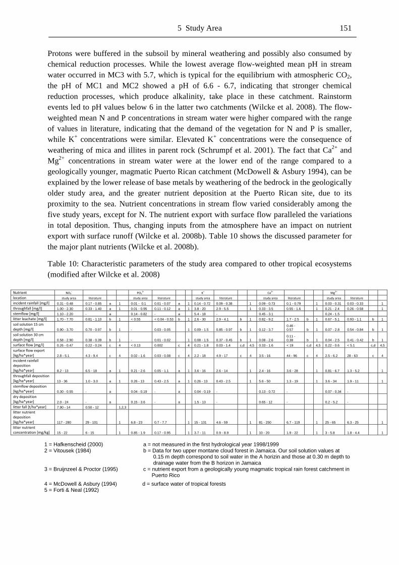
5 Study Area 151

Protons were buffered in the subsoil by mineral weathering and possibly also consumed by chemical reduction processes. While the lowest average flow-weighted mean pH in stream water occurred in MC3 with 5.7, which is typical for the equilibrium with atmospheric CO2, the pH of MC1 and MC2 showed a pH of 6.6 - 6.7, indicating that stronger chemical reduction processes, which produce alkalinity, take place in these catchment. Rainstorm events led to pH values below 6 in the latter two catchments (Wilcke et al. 2008). The flow-weighted mean N and P concentrations in stream water were higher compared with the range of values in literature, indicating that the demand of the vegetation for N and P is smaller, while K+ concentrations were similar. Elevated K+ concentrations were the consequence of weathering of mica and illites in parent rock (Schrumpf et al. 2001). The fact that Ca2+ and Mg2+ concentrations in stream water were at the lower end of the range compared to a geologically younger, magmatic Puerto Rican catchment (McDowell & Asbury 1994), can be explained by the lower release of base metals by weathering of the bedrock in the geologically older study area, and the greater nutrient deposition at the Puerto Rican site, due to its proximity to the sea. Nutrient concentrations in stream flow varied considerably among the five study years, except for N. The nutrient export with surface flow paralleled the variations in total deposition. Thus, changing inputs from the atmosphere have an impact on nutrient export with surface runoff (Wilcke et al. 2008b). Table 10 shows the discussed parameter for the major plant nutrients (Wilcke et al. 2008b).

Table 10: Characteristic parameters of the study area compared to other tropical ecosystems (modified after Wilcke et al. 2008)

�������� �3-� �� �� �� �4

3-� �� �� �� �+� �� �� �� �2+� �� �� �� ��2+� �� �� ��

�������� ����������� ����������� �� �� ����������� ����������� �� �� ����������� ����������� �� �� ����������� ����������� �� �� ����������� ����������� �� ��

���������������������� 0.31 - 0.48 0.17 - 0.85 a 1 0.01 - 0.1 0.01 - 0.07 a 1 0.14 - 0.72 0.09 - 0.38 1 0.09 - 0.73 0.1 - 0.79 1 0.03 - 0.31 0.03 - 0.33 1 ������������������� 1.00 - 2.30 0.33 - 1.40 a 1 0.01 - 0.95 0.11 - 0.12 a 1 3.8 - 20 2.9 - 5.5 1 0.33 - 3.5 0.55 - 1.6 1 0.21 - 2.4 0.26 - 0.58 1 ���������������� 1.10 - 2.20 - a 0.14 - 0.82 - a 5.4 - 18 - 0.45 - 3.1 0.24 - 1.5 ����������������������� 1.70 - 7.70 0.81 - 1.10 b 1 < 0.55 < 0.04 - 0.53 b 1 2.6 - 30 2.9 - 4.1 b 1 0.82 - 9.2 1.7 - 2.5 b 1 0.67 - 5.1 0.93 - 1.1 b 1 ��������������������� ���������� 0.90 - 3.70 0.70 - 0.97 b 1 - 0.03 - 0.05 1 0.09 - 1.5 0.85 - 0.97 b 1 0.12 - 3.7

0.46 - 0.57 b 1 0.07 - 2.8 0.54 - 0.84 b 1

�������������!"������ ���������� 0.58 - 2.90 0.38 - 0.39 b 1 - 0.01 - 0.02 1 0.08 - 1.5 0.37 - 0.45 b 1 0.08 - 2.6

0.11 - 0.38 b 1 0.04 - 2.5 0.41 - 0.42 b 1

�������������������� 0.26 - 0.47 0.22 - 0.24 c 4 < 0.13 0.002 c 4 0.21 - 1.8 0.03 - 1.4 c,d 4,5 0.33 - 1.6 < 19 c,d 4,5 0.22 - 0.6 < 5.1 c,d 4,5 ��������������# �����$����%������ 2.8 - 5.1 4.3 - 9.4 c 4 0.02 - 1.6 0.03 - 0.08 c 4 2.2 - 18 4.9 - 17 c 4 3.5 - 16 44 - 96 c 4 2.5 - 6.2 28 - 63 c 4 ����������������� ��������$����%������ 8.2 - 13 6.5 - 18 a 1 0.21 - 2.6 0.05 - 1.1 a 1 3.6 - 16 2.6 - 14 1 2.4 - 16 3.6 - 28 1 0.81 - 6.7 1.3 - 5.2 1 �������������� ��������$����%������ 13 - 36 1.0 - 3.0 a 1 0.26 - 13 0.43 - 2.5 a 1 0.26 - 13 0.43 - 2.5 1 5.6 - 50 1.3 - 19 1 3.6 - 34 1.9 - 11 1 ����������� ��������$����%������ 0.30 - 0.55 - a 0.04 - 0.19 - a 0.04 - 0.19 - 0.13 - 0.72 - 0.07 - 0.34 - ������ ��������$����%������ 2.0 - 24 - a 0.15 - 3.6 - a 1.5 - 13 - 0.65 - 12 - 0.2 - 5.2 - �����������������%������ 7.90 - 14 0.50 - 12 1,2,3 ���������������� ��������$����%������ 117 - 280 29 - 101 1 6.8 - 23 0.7 - 7.7 1 15 - 131 4.6 - 59 1 81 - 250 6.7 - 119 1 25 - 65 6.3 - 25 1 �����������������������������$��� 15 - 22 6 - 15 1 0.85 - 1.9 0.17 - 0.95 1 3.7 - 11 0.9 - 8.9 1 10 - 20 1.9 - 22 1 3 - 5.8 1.8 - 4.4 1

1 = Hafkenscheid (2000) a = not measured in the first hydrological year 1998/1999 2 = Vitousek (1984) b = Data for two upper montane cloud forest in Jamaica. Our soil solution values at 0.15 m depth correspond to soil water in the A horizin and those at 0.30 m depth to drainage water from the B horizon in Jamaica 3 = Bruijnzeel & Proctor (1995) c = nutrient export from a geologically young magmatic tropical rain forest catchment in Puerto Rico 4 = McDowell & Asbury (1994) d = surface water of tropical forests 5 = Forti & Neal (1992)

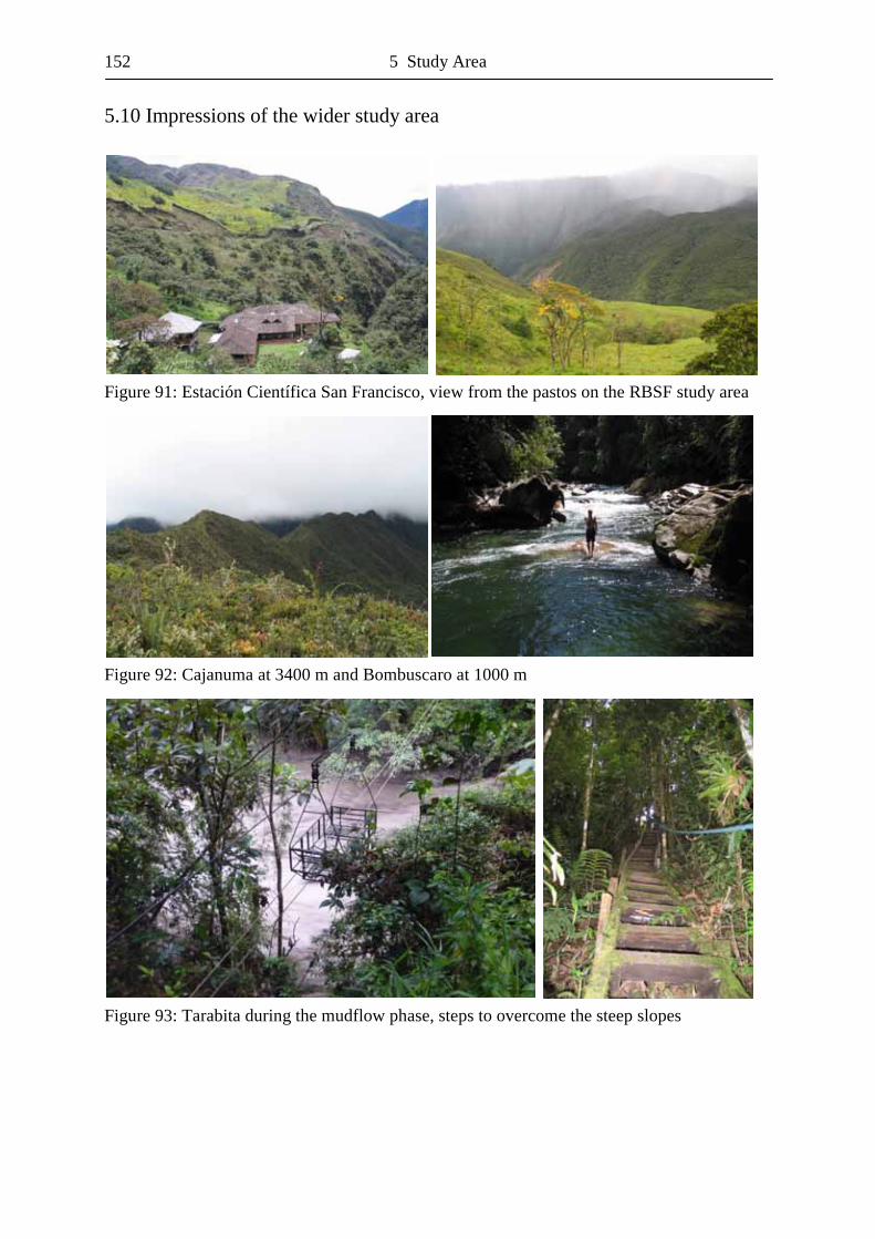
152 5 Study Area

5.10 Impressions of the wider study area

Figure 91: Estación Científica San Francisco, view from the pastos on the RBSF study area

Figure 92: Cajanuma at 3400 m and Bombuscaro at 1000 m

Figure 93: Tarabita during the mudflow phase, steps to overcome the steep slopes

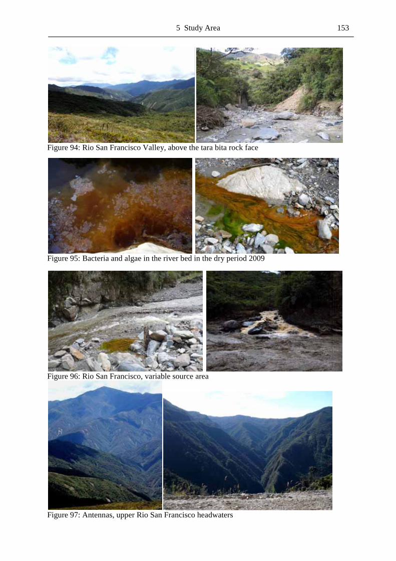
5 Study Area 153

Figure 94: Rio San Francisco Valley, above the tara bita rock face

Figure 95: Bacteria and algae in the river bed in the dry period 2009

Figure 96: Rio San Francisco, variable source area

Figure 97: Antennas, upper Rio San Francisco headwaters

154 5 Study Area

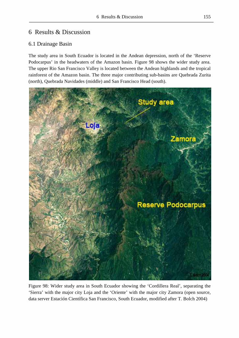
6 Results & Discussion 155

6 Results & Discussion

6.1 Drainage Basin

The study area in South Ecuador is located in the Andean depression, north of the ‘Reserve Podocarpus’ in the headwaters of the Amazon basin. Figure 98 shows the wider study area. The upper Rio San Francisco Valley is located between the Andean highlands and the tropical rainforest of the Amazon basin. The three major contributing sub-basins are Quebrada Zurita (north), Quebrada Navidades (middle) and San Francisco Head (south).

Figure 98: Wider study area in South Ecuador showing the ‘Cordillera Real’, separating the ‘Sierra’ with the major city Loja and the ‘Oriente’ with the major city Zamora (open source, data server Estación Científica San Francisco, South Ecuador, modified after T. Bolch 2004)

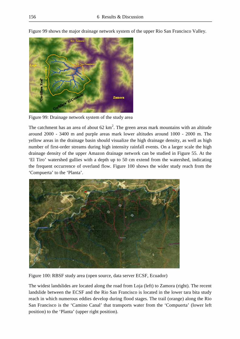
156 6 Results & Discussion

Figure 99 shows the major drainage network system of the upper Rio San Francisco Valley.

Figure 99: Drainage network system of the study area

The catchment has an area of about 62 km2. The green areas mark mountains with an altitude around 2000 - 3400 m and purple areas mark lower altitudes around 1000 - 2000 m. The yellow areas in the drainage basin should visualize the high drainage density, as well as high number of first-order streams during high intensity rainfall events. On a larger scale the high drainage density of the upper Amazon drainage network can be studied in Figure 55. At the ‘El Tiro’ watershed gullies with a depth up to 50 cm extend from the watershed, indicating the frequent occurrence of overland flow. Figure 100 shows the wider study reach from the ‘Compuerta’ to the ‘Planta’.

Figure 100: RBSF study area (open source, data server ECSF, Ecuador)

The widest landslides are located along the road from Loja (left) to Zamora (right). The recent landslide between the ECSF and the Rio San Francisco is located in the lower tara bita study reach in which numerous eddies develop during flood stages. The trail (orange) along the Rio San Francisco is the ‘Camino Canal’ that transports water from the ‘Compuerta’ (lower left position) to the ‘Planta’ (upper right position).

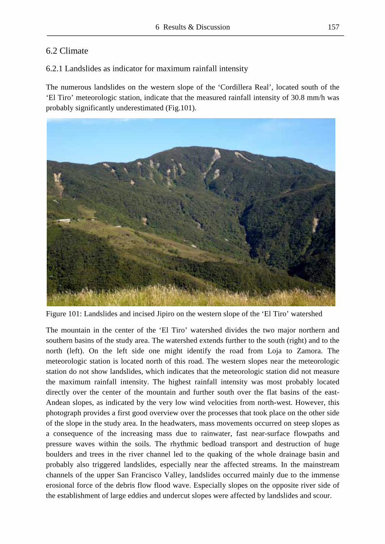
6 Results & Discussion 157

6.2 Climate

6.2.1 Landslides as indicator for maximum rainfall intensity

The numerous landslides on the western slope of the ‘Cordillera Real’, located south of the ‘El Tiro’ meteorologic station, indicate that the measured rainfall intensity of 30.8 mm/h was probably significantly underestimated (Fig.101).

Figure 101: Landslides and incised Jipiro on the western slope of the ‘El Tiro’ watershed

The mountain in the center of the ‘El Tiro’ watershed divides the two major northern and southern basins of the study area. The watershed extends further to the south (right) and to the north (left). On the left side one might identify the road from Loja to Zamora. The meteorologic station is located north of this road. The western slopes near the meteorologic station do not show landslides, which indicates that the meteorologic station did not measure the maximum rainfall intensity. The highest rainfall intensity was most probably located directly over the center of the mountain and further south over the flat basins of the east-Andean slopes, as indicated by the very low wind velocities from north-west. However, this photograph provides a first good overview over the processes that took place on the other side of the slope in the study area. In the headwaters, mass movements occurred on steep slopes as a consequence of the increasing mass due to rainwater, fast near-surface flowpaths and pressure waves within the soils. The rhythmic bedload transport and destruction of huge boulders and trees in the river channel led to the quaking of the whole drainage basin and probably also triggered landslides, especially near the affected streams. In the mainstream channels of the upper San Francisco Valley, landslides occurred mainly due to the immense erosional force of the debris flow flood wave. Especially slopes on the opposite river side of the establishment of large eddies and undercut slopes were affected by landslides and scour.

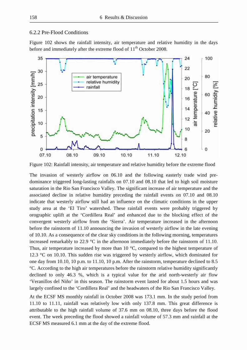
158 6 Results & Discussion

6.2.2 Pre-Flood Conditions

Figure 102 shows the rainfall intensity, air temperature and relative humidity in the days before and immediately after the extreme flood of 11th October 2008.

Figure 102: Rainfall intensity, air temperature and relative humidity before the extreme flood

The invasion of westerly airflow on 06.10 and the following easterly trade wind pre-dominance triggered long-lasting rainfalls on 07.10 and 08.10 that led to high soil moisture saturation in the Rio San Francisco Valley. The significant increase of air temperature and the associated decline in relative humidity preceding the rainfall events on 07.10 and 08.10 indicate that westerly airflow still had an influence on the climatic conditions in the upper study area at the ‘El Tiro’ watershed. These rainfall events were probably triggered by orographic uplift at the ‘Cordillera Real’ and enhanced due to the blocking effect of the convergent westerly airflow from the ‘Sierra’. Air temperature increased in the afternoon before the rainstorm of 11.10 announcing the invasion of westerly airflow in the late evening of 10.10. As a consequence of the clear sky conditions in the following morning, temperatures increased remarkably to 22.9 °C in the afternoon immediately before the rainstorm of 11.10. Thus, air temperature increased by more than 10 °C, compared to the highest temperature of 12.3 °C on 10.10. This sudden rise was triggered by westerly airflow, which dominated for one day from 10.10, 10 p.m. to 11.10, 10 p.m. After the rainstorm, temperature declined to 8.5 °C. According to the high air temperatures before the rainstorm relative humidity significantly declined to only 46.3 %, which is a typical value for the arid north-westerly air flow ‘Veranillos del Niño’ in this season. The rainstorm event lasted for about 1.5 hours and was largely confined to the ‘Cordillera Real’ and the headwaters of the Rio San Francisco Valley.

At the ECSF MS monthly rainfall in October 2008 was 173.1 mm. In the study period from 11.10 to 11.11, rainfall was relatively low with only 137.8 mm. This great difference is attributable to the high rainfall volume of 37.6 mm on 08.10, three days before the flood event. The week preceding the flood showed a rainfall volume of 57.3 mm and rainfall at the ECSF MS measured 6.1 mm at the day of the extreme flood.

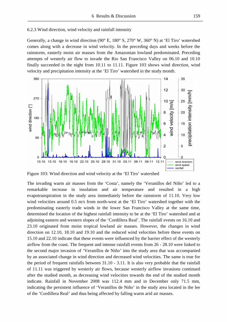
6 Results & Discussion 159

6.2.3 Wind direction, wind velocity and rainfall intensity

Generally, a change in wind direction (90° E, 180° S, 270° W, 360° N) at ‘El Tiro’ watershed comes along with a decrease in wind velocity. In the preceding days and weeks before the rainstorm, easterly moist air masses from the Amazonian lowland predominated. Preceding attempts of westerly air flow to invade the Rio San Francisco Valley on 06.10 and 10.10 finally succeeded in the night from 10.11 to 11.11. Figure 103 shows wind direction, wind velocity and precipitation intensity at the ‘El Tiro’ watershed in the study month.

Figure 103: Wind direction and wind velocity at the ‘El Tiro’ watershed

The invading warm air masses from the ‘Costa’, namely the ‘Veranillos del Niño’ led to a remarkable increase in insolation and air temperature and resulted in a high evapotranspiration in the study area immediately before the rainstorm of 11.10. Very low wind velocities around 0.5 m/s from north-west at the ‘El Tiro’ watershed together with the predominating easterly trade winds in the lower San Francisco Valley at the same time, determined the location of the highest rainfall intensity to be at the ‘El Tiro’ watershed and at adjoining eastern and western slopes of the ‘Cordillera Real’. The rainfall events on 16.10 and 23.10 originated from moist tropical lowland air masses. However, the changes in wind direction on 12.10, 18.10 and 19.10 and the reduced wind velocities before these events on 15.10 and 22.10 indicate that these events were influenced by the barrier effect of the westerly airflow from the coast. The frequent and intense rainfall events from 26 - 28.10 were linked to the second major invasion of ‘Veranillos de Niño’ into the study area that was accompanied by an associated change in wind direction and decreased wind velocities. The same is true for the period of frequent rainfalls between 31.10 - 3.11. It is also very probable that the rainfall of 11.11 was triggered by westerly air flows, because westerly airflow invasions continued after the studied month, as decreasing wind velocities towards the end of the studied month indicate. Rainfall in November 2008 was 112.4 mm and in December only 71.5 mm, indicating the persistent influence of ‘Veranillos de Niño’ in the study area located in the lee of the ‘Cordillera Real’ and thus being affected by falling warm arid air masses.

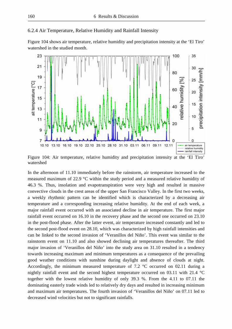
160 6 Results & Discussion

6.2.4 Air Temperature, Relative Humidity and Rainfall Intensity

Figure 104 shows air temperature, relative humidity and precipitation intensity at the ‘El Tiro’ watershed in the studied month.

Figure 104: Air temperature, relative humidity and precipitation intensity at the ‘El Tiro’ watershed

In the afternoon of 11.10 immediately before the rainstorm, air temperature increased to the measured maximum of 22.9 °C within the study period and a measured relative humidity of 46.3 %. Thus, insolation and evapotranspiration were very high and resulted in massive convective clouds in the crest areas of the upper San Francisco Valley. In the first two weeks, a weekly rhythmic pattern can be identified which is characterized by a decreasing air temperature and a corresponding increasing relative humidity. At the end of each week, a major rainfall event occurred with an associated decline in air temperature. The first major rainfall event occurred on 16.10 in the recovery phase and the second one occurred on 23.10 in the post-flood phase. After the latter event, air temperature increased constantly and led to the second post-flood event on 28.10, which was characterized by high rainfall intensities and can be linked to the second invasion of ‘Veranillos del Niño’. This event was similar to the rainstorm event on 11.10 and also showed declining air temperatures thereafter. The third major invasion of ‘Veranillos del Niño’ into the study area on 31.10 resulted in a tendency towards increasing maximum and minimum temperatures as a consequence of the prevailing good weather conditions with sunshine during daylight and absence of clouds at night. Accordingly, the minimum measured temperature of 7.2 °C occurred on 02.11 during a nightly rainfall event and the second highest temperature occurred on 03.11 with 21.4 °C together with the lowest relative humidity of only 39.3 %. From the 4.11 to 07.11 the dominating easterly trade winds led to relatively dry days and resulted in increasing minimum and maximum air temperatures. The fourth invasion of ‘Veranillos del Niño’ on 07.11 led to decreased wind velocities but not to significant rainfalls.

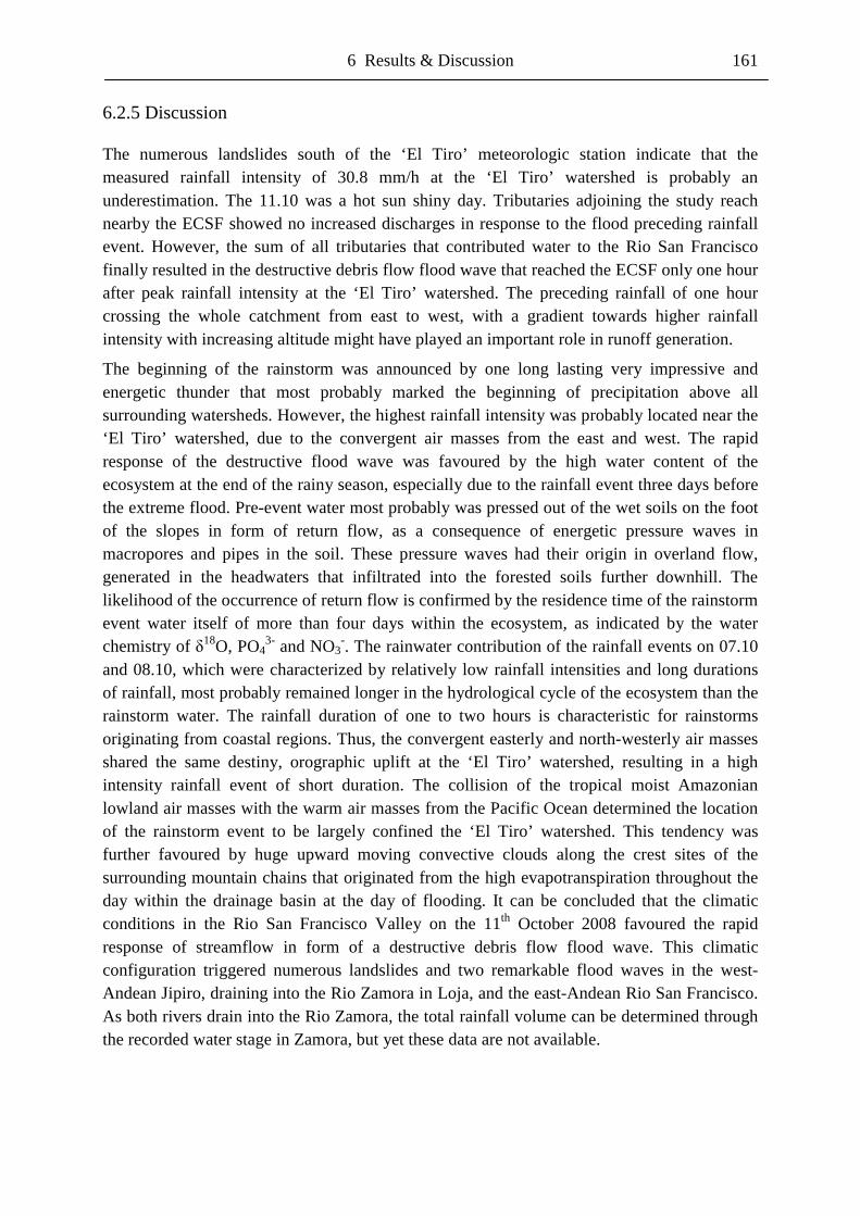
6 Results & Discussion 161

6.2.5 Discussion

The numerous landslides south of the ‘El Tiro’ meteorologic station indicate that the measured rainfall intensity of 30.8 mm/h at the ‘El Tiro’ watershed is probably an underestimation. The 11.10 was a hot sun shiny day. Tributaries adjoining the study reach nearby the ECSF showed no increased discharges in response to the flood preceding rainfall event. However, the sum of all tributaries that contributed water to the Rio San Francisco finally resulted in the destructive debris flow flood wave that reached the ECSF only one hour after peak rainfall intensity at the ‘El Tiro’ watershed. The preceding rainfall of one hour crossing the whole catchment from east to west, with a gradient towards higher rainfall intensity with increasing altitude might have played an important role in runoff generation.

The beginning of the rainstorm was announced by one long lasting very impressive and energetic thunder that most probably marked the beginning of precipitation above all surrounding watersheds. However, the highest rainfall intensity was probably located near the ‘El Tiro’ watershed, due to the convergent air masses from the east and west. The rapid response of the destructive flood wave was favoured by the high water content of the ecosystem at the end of the rainy season, especially due to the rainfall event three days before the extreme flood. Pre-event water most probably was pressed out of the wet soils on the foot of the slopes in form of return flow, as a consequence of energetic pressure waves in macropores and pipes in the soil. These pressure waves had their origin in overland flow, generated in the headwaters that infiltrated into the forested soils further downhill. The likelihood of the occurrence of return flow is confirmed by the residence time of the rainstorm event water itself of more than four days within the ecosystem, as indicated by the water chemistry of �18O, PO4

3- and NO3-. The rainwater contribution of the rainfall events on 07.10

and 08.10, which were characterized by relatively low rainfall intensities and long durations of rainfall, most probably remained longer in the hydrological cycle of the ecosystem than the rainstorm water. The rainfall duration of one to two hours is characteristic for rainstorms originating from coastal regions. Thus, the convergent easterly and north-westerly air masses shared the same destiny, orographic uplift at the ‘El Tiro’ watershed, resulting in a high intensity rainfall event of short duration. The collision of the tropical moist Amazonian lowland air masses with the warm air masses from the Pacific Ocean determined the location of the rainstorm event to be largely confined the ‘El Tiro’ watershed. This tendency was further favoured by huge upward moving convective clouds along the crest sites of the surrounding mountain chains that originated from the high evapotranspiration throughout the day within the drainage basin at the day of flooding. It can be concluded that the climatic conditions in the Rio San Francisco Valley on the 11th October 2008 favoured the rapid response of streamflow in form of a destructive debris flow flood wave. This climatic configuration triggered numerous landslides and two remarkable flood waves in the west-Andean Jipiro, draining into the Rio Zamora in Loja, and the east-Andean Rio San Francisco. As both rivers drain into the Rio Zamora, the total rainfall volume can be determined through the recorded water stage in Zamora, but yet these data are not available.

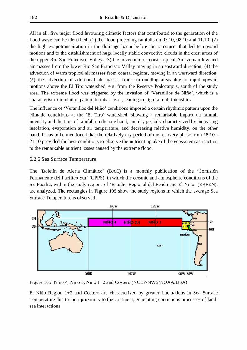
162 6 Results & Discussion

All in all, five major flood favouring climatic factors that contributed to the generation of the flood wave can be identified: (1) the flood preceding rainfalls on 07.10, 08.10 and 11.10; (2) the high evapotranspiration in the drainage basin before the rainstorm that led to upward motions and to the establishment of huge locally stable convective clouds in the crest areas of the upper Rio San Francisco Valley; (3) the advection of moist tropical Amazonian lowland air masses from the lower Rio San Francisco Valley moving in an eastward direction; (4) the advection of warm tropical air masses from coastal regions, moving in an westward direction; (5) the advection of additional air masses from surrounding areas due to rapid upward motions above the El Tiro watershed, e.g. from the Reserve Podocarpus, south of the study area. The extreme flood was triggered by the invasion of ‘Veranillos de Niño’, which is a characteristic circulation pattern in this season, leading to high rainfall intensities.

The influence of ‘Veranillos del Niño’ conditions imposed a certain rhythmic pattern upon the climatic conditions at the ‘El Tiro’ watershed, showing a remarkable impact on rainfall intensity and the time of rainfall on the one hand, and dry periods, characterized by increasing insolation, evaporation and air temperature, and decreasing relative humidity, on the other hand. It has to be mentioned that the relatively dry period of the recovery phase from 18.10 - 21.10 provided the best conditions to observe the nutrient uptake of the ecosystem as reaction to the remarkable nutrient losses caused by the extreme flood.

6.2.6 Sea Surface Temperature

The ‘Boletín de Alerta Climático’ (BAC) is a monthly publication of the ‘Comisión Permanente del Pacífico Sur’ (CPPS), in which the oceanic and atmospheric conditions of the SE Pacific, within the study regions of ‘Estudio Regional del Fenómeno El Niño’ (ERFEN), are analyzed. The rectangles in Figure 105 show the study regions in which the average Sea Surface Temperature is observed.

Figure 105: Niño 4, Niño 3, Niño 1+2 and Costero (NCEP/NWS/NOAA/USA)

El Niño Region 1+2 and Costero are characterized by greater fluctuations in Sea Surface Temperature due to their proximity to the continent, generating continuous processes of land-sea interactions.

6 Results & Discussion 163

The Sea Surface Temperature anomalies for the study region Costero at the Ecuadorian and Peruvian coast are illustrated in Figure 106 (NCEP/NWS/NOAA/USA).

Figure 106: Sea Surface Temperature anomalies for Costero area (NCEP/NWS/NOAA/USA)

Sea Surface Temperature was relatively high between February and April 2008 when major flooding affected coastal regions in Ecuador. The Spanish article ‘Reportaje Grafico Sobre las Inundaciones en Ecuador Febrero-Abril 2008’ provides good informations on these floods that can be viewed on www.calameo.com. The extreme flood occurred at the end of the second peak phase of positive Sea Surface Temperature anomaly in October 2008.

According to the Oceanographic Institute of the Navy of Ecuador (INOCAR), air temperature in the Ecuadorian coast fluctuated between 23.2 ºC and 26.3 ºC with anomalies between -0.2 ºC and 1.0 ºC during September 2008. Sea Surface Temperature varied between 23.4 and 26.7 ºC with anomalies between 0.2 and 1.0 ºC. Monthly rainfall in the Ecuadorian Coast ranged between 0 - 10 mm. The oceanographic cruise of the ‘BAE Orión’ showed that Sea Surface Temperature in September 2009 fluctuated from 20.5 °C in the south to 25.5 ºC in the north with positive anomalies between 0.5 and 1.0 ºC for a large extent of the cruise area. The Equatorial Front showed a weak thermohaline gradient that was possibly accompanied by a weak incursion of the cold Humboldt Current towards equatorial regions. In the first 50 m below the sea level, increasing temperatures in the Eastern Pacific regions have been observed but did not reach alarming values or show signals of anomalous process development.

During October 2008, air temperature in the Ecuadorian coast fluctuated between 22.4 ºC and 26.0 ºC with anomalies between 0 ºC and 0.7 ºC. Sea Surface Temperature fluctuated between 22.5 and 26.4 ºC with anomalies between -1.3 and 0.5 ºC. Monthly rainfall in the Northern Ecuadorian coast was 30 mm with a positive anomaly of 18 % that was influenced by the loosening of convective nuclei originating from the ITCZ. Rainfall volume in the Ecuadorian Coast was very low and wind direction was South South-East.

During November 2008, air temperature in the Ecuadorian coast fluctuated between 23.5 ºC and 26.0 ºC with anomalies of -0.3 ºC. Sea Surface Temperature fluctuated between 23.8 ºC and 26.3 ºC with anomalies of -0.3 and 0.5 ºC. Monthly rainfall in the northern regions the Ecuadorian coast measured 97 mm with a positive anomaly of 10% that was influenced by the loosening of convective nuclei originating from ITCZ. Other parts of Ecuador remained mostly dry. The wind direction was South South-East.

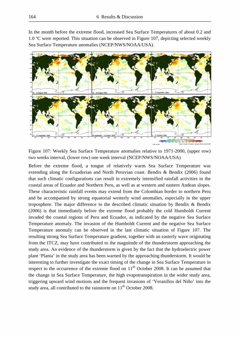
164 6 Results & Discussion

In the month before the extreme flood, increased Sea Surface Temperatures of about 0.2 and 1.0 ºC were reported. This situation can be observed in Figure 107, depicting selected weekly Sea Surface Temperature anomalies (NCEP/NWS/NOAA/USA).

Figure 107: Weekly Sea Surface Temperature anomalies relative to 1971-2000, (upper row) two weeks interval, (lower row) one week interval (NCEP/NWS/NOAA/USA)

Before the extreme flood, a tongue of relatively warm Sea Surface Temperature was extending along the Ecuadorian and North Peruvian coast. Bendix & Bendix (2006) found that such climatic configurations can result in extremely intensified rainfall activities in the coastal areas of Ecuador and Northern Peru, as well as at western and eastern Andean slopes. These characteristic rainfall events may extend from the Colombian border to northern Peru and be accompanied by strong equatorial westerly wind anomalies, especially in the upper troposphere. The major difference to the described climatic situation by Bendix & Bendix (2006) is that immediately before the extreme flood probably the cold Humboldt Current invaded the coastal regions of Peru and Ecuador, as indicated by the negative Sea Surface Temperature anomaly. The invasion of the Humboldt Current and the negative Sea Surface Temperature anomaly can be observed in the last climatic situation of Figure 107. The resulting strong Sea Surface Temperature gradient, together with an easterly wave originating from the ITCZ, may have contributed to the magnitude of the thunderstorm approaching the study area. An evidence of the thunderstorm is given by the fact that the hydroelectric power plant ‘Planta’ in the study area has been warned by the approaching thunderstorm. It would be interesting to further investigate the exact timing of the change in Sea Surface Temperature in respect to the occurrence of the extreme flood on 11th October 2008. It can be assumed that the change in Sea Surface Temperature, the high evapotranspiration in the wider study area, triggering upward wind motions and the frequent invasions of ‘Veranillos del Niño’ into the study area, all contributed to the rainstorm on 11th October 2008.

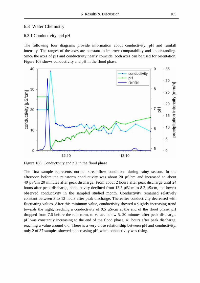
6 Results & Discussion 165

6.3 Water Chemistry

6.3.1 Conductivity and pH

The following four diagrams provide information about conductivity, pH and rainfall intensity. The ranges of the axes are constant to improve comparability and understanding. Since the axes of pH and conductivity nearly coincide, both axes can be used for orientation. Figure 108 shows conductivity and pH in the flood phase.

Figure 108: Conductivity and pH in the flood phase

The first sample represents normal streamflow conditions during rainy season. In the afternoon before the rainstorm conductivity was about 20 µS/cm and increased to about 40 µS/cm 20 minutes after peak discharge. From about 2 hours after peak discharge until 24 hours after peak discharge, conductivity declined from 13.3 µS/cm to 8.2 µS/cm, the lowest observed conductivity in the sampled studied month. Conductivity remained relatively constant between 3 to 12 hours after peak discharge. Thereafter conductivity decreased with fluctuating values. After this minimum value, conductivity showed a slightly increasing trend towards the night, reaching a conductivity of 9.5 µS/cm at the end of the flood phase. pH dropped from 7.6 before the rainstorm, to values below 5, 20 minutes after peak discharge. pH was constantly increasing to the end of the flood phase, 41 hours after peak discharge, reaching a value around 6.6. There is a very close relationship between pH and conductivity, only 2 of 37 samples showed a decreasing pH, when conductivity was rising.

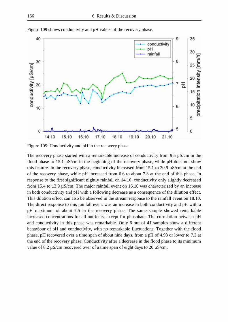
166 6 Results & Discussion

Figure 109 shows conductivity and pH values of the recovery phase.

Figure 109: Conductivity and pH in the recovery phase

The recovery phase started with a remarkable increase of conductivity from 9.5 µS/cm in the flood phase to 15.1 µS/cm in the beginning of the recovery phase, while pH does not show this feature. In the recovery phase, conductivity increased from 15.1 to 20.9 µS/cm at the end of the recovery phase, while pH increased from 6.6 to about 7.3 at the end of this phase. In response to the first significant nightly rainfall on 14.10, conductivity only slightly decreased from 15.4 to 13.9 µS/cm. The major rainfall event on 16.10 was characterized by an increase in both conductivity and pH with a following decrease as a consequence of the dilution effect. This dilution effect can also be observed in the stream response to the rainfall event on 18.10. The direct response to this rainfall event was an increase in both conductivity and pH with a pH maximum of about 7.5 in the recovery phase. The same sample showed remarkable increased concentrations for all nutrients, except for phosphate. The correlation between pH and conductivity in this phase was remarkable. Only 6 out of 41 samples show a different behaviour of pH and conductivity, with no remarkable fluctuations. Together with the flood phase, pH recovered over a time span of about nine days, from a pH of 4.93 or lower to 7.3 at the end of the recovery phase. Conductivity after a decrease in the flood phase to its minimum value of 8.2 µS/cm recovered over of a time span of eight days to 20 µS/cm.

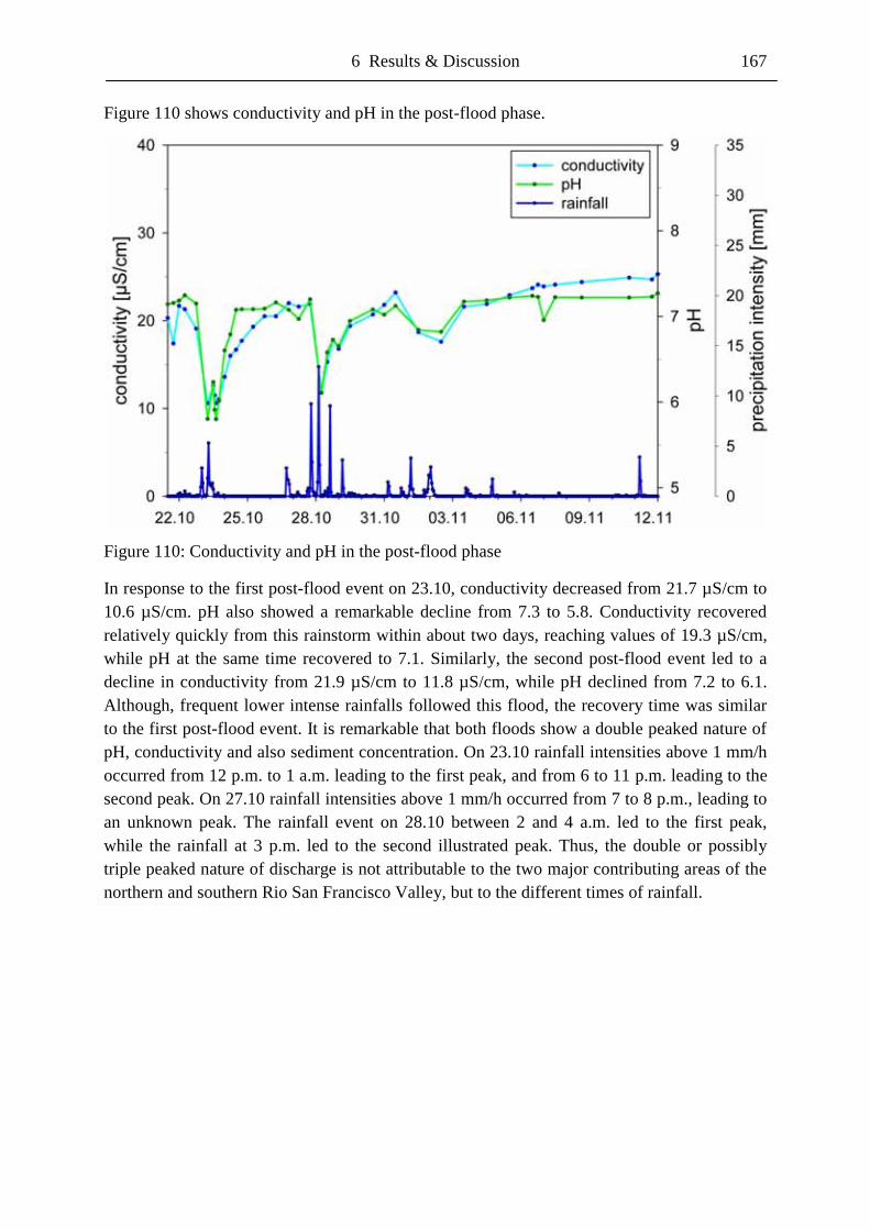
6 Results & Discussion 167

Figure 110 shows conductivity and pH in the post-flood phase.

Figure 110: Conductivity and pH in the post-flood phase

In response to the first post-flood event on 23.10, conductivity decreased from 21.7 µS/cm to 10.6 µS/cm. pH also showed a remarkable decline from 7.3 to 5.8. Conductivity recovered relatively quickly from this rainstorm within about two days, reaching values of 19.3 µS/cm, while pH at the same time recovered to 7.1. Similarly, the second post-flood event led to a decline in conductivity from 21.9 µS/cm to 11.8 µS/cm, while pH declined from 7.2 to 6.1. Although, frequent lower intense rainfalls followed this flood, the recovery time was similar to the first post-flood event. It is remarkable that both floods show a double peaked nature of pH, conductivity and also sediment concentration. On 23.10 rainfall intensities above 1 mm/h occurred from 12 p.m. to 1 a.m. leading to the first peak, and from 6 to 11 p.m. leading to the second peak. On 27.10 rainfall intensities above 1 mm/h occurred from 7 to 8 p.m., leading to an unknown peak. The rainfall event on 28.10 between 2 and 4 a.m. led to the first peak, while the rainfall at 3 p.m. led to the second illustrated peak. Thus, the double or possibly triple peaked nature of discharge is not attributable to the two major contributing areas of the northern and southern Rio San Francisco Valley, but to the different times of rainfall.

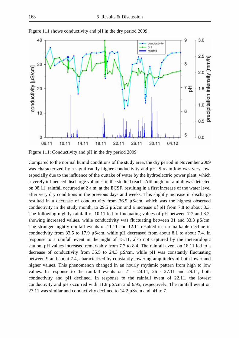
168 6 Results & Discussion

Figure 111 shows conductivity and pH in the dry period 2009.

Figure 111: Conductivity and pH in the dry period 2009

Compared to the normal humid conditions of the study area, the dry period in November 2009 was characterized by a significantly higher conductivity and pH. Streamflow was very low, especially due to the influence of the outtake of water by the hydroelectric power plant, which severely influenced discharge volumes in the studied reach. Although no rainfall was detected on 08.11, rainfall occurred at 2 a.m. at the ECSF, resulting in a first increase of the water level after very dry conditions in the previous days and weeks. This slightly increase in discharge resulted in a decrease of conductivity from 36.9 µS/cm, which was the highest observed conductivity in the study month, to 29.5 µS/cm and a increase of pH from 7.8 to about 8.3. The following nightly rainfall of 10.11 led to fluctuating values of pH between 7.7 and 8.2, showing increased values, while conductivity was fluctuating between 31 and 33.3 µS/cm. The stronger nightly rainfall events of 11.11 and 12.11 resulted in a remarkable decline in conductivity from 33.5 to 17.9 µS/cm, while pH decreased from about 8.1 to about 7.4. In response to a rainfall event in the night of 15.11, also not captured by the meteorologic station, pH values increased remarkably from 7.7 to 8.4. The rainfall event on 18.11 led to a decrease of conductivity from 35.5 to 24.3 µS/cm, while pH was constantly fluctuating between 9 and about 7.4, characterized by constantly lowering amplitudes of both lower and higher values. This phenomenon changed in an hourly rhythmic pattern from high to low values. In response to the rainfall events on 21 - 24.11, 26 - 27.11 and 29.11, both conductivity and pH declined. In response to the rainfall event of 22.11, the lowest conductivity and pH occurred with 11.8 µS/cm and 6.95, respectively. The rainfall event on 27.11 was similar and conductivity declined to 14.2 µS/cm and pH to 7.

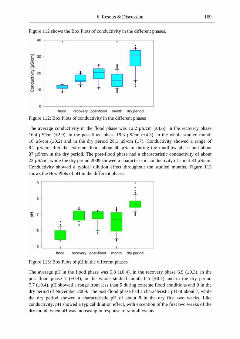
6 Results & Discussion 169

Figure 112 shows the Box Plots of conductivity in the different phases.

Figure 112: Box Plots of conductivity in the different phases

The average conductivity in the flood phase was 12.2 µS/cm (±4.6), in the recovery phase 16.4 µS/cm (±2.9), in the post-flood phase 19.3 µS/cm (±4.3), in the whole studied month 16 µS/cm (±0.2) and in the dry period 28.1 µS/cm (±7). Conductivity showed a range of 8.2 µS/cm after the extreme flood, about 40 µS/cm during the mudflow phase and about 37 µS/cm in the dry period. The post-flood phase had a characteristic conductivity of about 22 µS/cm, while the dry period 2009 showed a characteristic conductivity of about 33 µS/cm. Conductivity showed a typical dilution effect throughout the studied months. Figure 113 shows the Box Plots of pH in the different phases.

Figure 113: Box Plots of pH in the different phases

The average pH in the flood phase was 5.8 (±0.4), in the recovery phase 6.9 (±0.3), in the post-flood phase 7 (±0.4), in the whole studied month 6.5 (±0.7) and in the dry period 7.7 (±0.4). pH showed a range from less than 5 during extreme flood conditions and 9 in the dry period of November 2009. The post-flood phase had a characteristic pH of about 7, while the dry period showed a characteristic pH of about 8 in the dry first two weeks. Like conductivity, pH showed a typical dilution effect, with exception of the first two weeks of the dry month when pH was increasing in response to rainfall events.

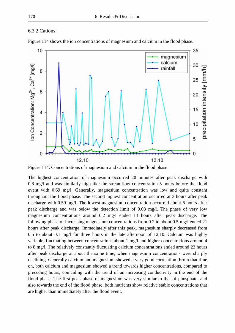
170 6 Results & Discussion

6.3.2 Cations Figure 114 shows the ion concentrations of magnesium and calcium in the flood phase.

Figure 114: Concentrations of magnesium and calcium in the flood phase

The highest concentration of magnesium occurred 20 minutes after peak discharge with 0.8 mg/l and was similarly high like the streamflow concentration 5 hours before the flood event with 0.69 mg/l. Generally, magnesium concentration was low and quite constant throughout the flood phase. The second highest concentration occurred at 3 hours after peak discharge with 0.59 mg/l. The lowest magnesium concentration occurred about 6 hours after peak discharge and was below the detection limit of 0.03 mg/l. The phase of very low magnesium concentrations around 0.2 mg/l ended 13 hours after peak discharge. The following phase of increasing magnesium concentrations from 0.2 to about 0.5 mg/l ended 21 hours after peak discharge. Immediately after this peak, magnesium sharply decreased from 0.5 to about 0.1 mg/l for three hours in the late afternoon of 12.10. Calcium was highly variable, fluctuating between concentrations about 1 mg/l and higher concentrations around 4 to 8 mg/l. The relatively constantly fluctuating calcium concentrations ended around 23 hours after peak discharge at about the same time, when magnesium concentrations were sharply declining. Generally calcium and magnesium showed a very good correlation. From that time on, both calcium and magnesium showed a trend towards higher concentrations, compared to preceding hours, coinciding with the trend of an increasing conductivity in the end of the flood phase. The first peak phase of magnesium was very similar to that of phosphate, and also towards the end of the flood phase, both nutrients show relative stable concentrations that are higher than immediately after the flood event.

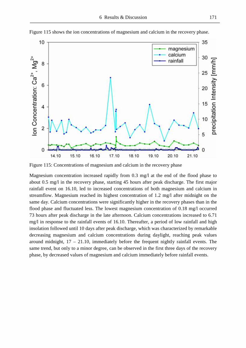
6 Results & Discussion 171

Figure 115 shows the ion concentrations of magnesium and calcium in the recovery phase.

Figure 115: Concentrations of magnesium and calcium in the recovery phase

Magnesium concentration increased rapidly from 0.3 mg/l at the end of the flood phase to about 0.5 mg/l in the recovery phase, starting 45 hours after peak discharge. The first major rainfall event on 16.10, led to increased concentrations of both magnesium and calcium in streamflow. Magnesium reached its highest concentration of 1.2 mg/l after midnight on the same day. Calcium concentrations were significantly higher in the recovery phases than in the flood phase and fluctuated less. The lowest magnesium concentration of 0.18 mg/l occurred 73 hours after peak discharge in the late afternoon. Calcium concentrations increased to 6.71 mg/l in response to the rainfall events of 16.10. Thereafter, a period of low rainfall and high insolation followed until 10 days after peak discharge, which was characterized by remarkable decreasing magnesium and calcium concentrations during daylight, reaching peak values around midnight, 17 – 21.10, immediately before the frequent nightly rainfall events. The same trend, but only to a minor degree, can be observed in the first three days of the recovery phase, by decreased values of magnesium and calcium immediately before rainfall events.

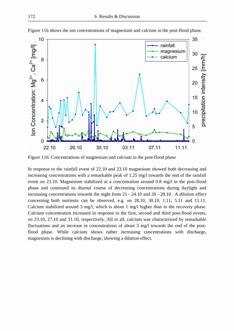
172 6 Results & Discussion

Figure 116 shows the ion concentrations of magnesium and calcium in the post-flood phase.

Figure 116: Concentrations of magnesium and calcium in the post-flood phase In response to the rainfall event of 22.10 and 23.10 magnesium showed both decreasing and increasing concentrations with a remarkable peak of 1.25 mg/l towards the end of the rainfall event on 23.10. Magnesium stabilized at a concentration around 0.8 mg/l in the post-flood phase and continued its diurnal course of decreasing concentrations during daylight and increasing concentrations towards the night from 21 - 24.10 and 26 - 28.10. A dilution effect concerning both nutrients can be observed, e.g. on 28.10, 30.10, 1.11, 5.11 and 11.11. Calcium stabilized around 3 mg/l, which is about 1 mg/l higher than in the recovery phase. Calcium concentration increased in response to the first, second and third post-flood events, on 23.10, 27.10 and 31.10, respectively. All in all, calcium was characterized by remarkable fluctuations and an increase in concentrations of about 3 mg/l towards the end of the post-flood phase. While calcium shows rather increasing concentrations with discharge, magnesium is declining with discharge, showing a dilution effect.

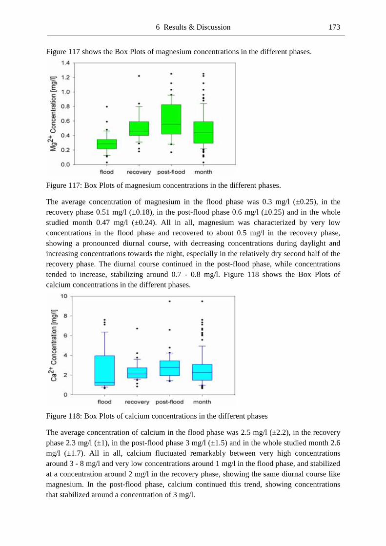
6 Results & Discussion 173

Figure 117 shows the Box Plots of magnesium concentrations in the different phases.

Figure 117: Box Plots of magnesium concentrations in the different phases.

The average concentration of magnesium in the flood phase was 0.3 mg/l (±0.25), in the recovery phase 0.51 mg/l (±0.18), in the post-flood phase 0.6 mg/l (±0.25) and in the whole studied month 0.47 mg/l (±0.24). All in all, magnesium was characterized by very low concentrations in the flood phase and recovered to about 0.5 mg/l in the recovery phase, showing a pronounced diurnal course, with decreasing concentrations during daylight and increasing concentrations towards the night, especially in the relatively dry second half of the recovery phase. The diurnal course continued in the post-flood phase, while concentrations tended to increase, stabilizing around 0.7 - 0.8 mg/l. Figure 118 shows the Box Plots of calcium concentrations in the different phases.

Figure 118: Box Plots of calcium concentrations in the different phases

The average concentration of calcium in the flood phase was 2.5 mg/l (±2.2), in the recovery phase 2.3 mg/l (±1), in the post-flood phase 3 mg/l (±1.5) and in the whole studied month 2.6 mg/l (±1.7). All in all, calcium fluctuated remarkably between very high concentrations around 3 - 8 mg/l and very low concentrations around 1 mg/l in the flood phase, and stabilized at a concentration around 2 mg/l in the recovery phase, showing the same diurnal course like magnesium. In the post-flood phase, calcium continued this trend, showing concentrations that stabilized around a concentration of 3 mg/l.

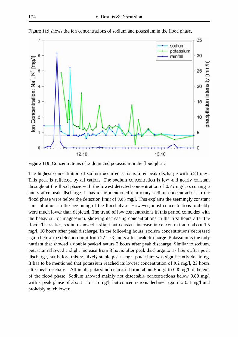
174 6 Results & Discussion

Figure 119 shows the ion concentrations of sodium and potassium in the flood phase.

Figure 119: Concentrations of sodium and potassium in the flood phase

The highest concentration of sodium occurred 3 hours after peak discharge with 5.24 mg/l. This peak is reflected by all cations. The sodium concentration is low and nearly constant throughout the flood phase with the lowest detected concentration of 0.75 mg/l, occurring 6 hours after peak discharge. It has to be mentioned that many sodium concentrations in the flood phase were below the detection limit of 0.83 mg/l. This explains the seemingly constant concentrations in the beginning of the flood phase. However, most concentrations probably were much lower than depicted. The trend of low concentrations in this period coincides with the behaviour of magnesium, showing decreasing concentrations in the first hours after the flood. Thereafter, sodium showed a slight but constant increase in concentration to about 1.5 mg/l, 18 hours after peak discharge. In the following hours, sodium concentrations decreased again below the detection limit from 22 - 23 hours after peak discharge. Potassium is the only nutrient that showed a double peaked nature 3 hours after peak discharge. Similar to sodium, potassium showed a slight increase from 8 hours after peak discharge to 17 hours after peak discharge, but before this relatively stable peak stage, potassium was significantly declining. It has to be mentioned that potassium reached its lowest concentration of 0.2 mg/l, 23 hours after peak discharge. All in all, potassium decreased from about 5 mg/l to 0.8 mg/l at the end of the flood phase. Sodium showed mainly not detectable concentrations below 0.83 mg/l with a peak phase of about 1 to 1.5 mg/l, but concentrations declined again to 0.8 mg/l and probably much lower.

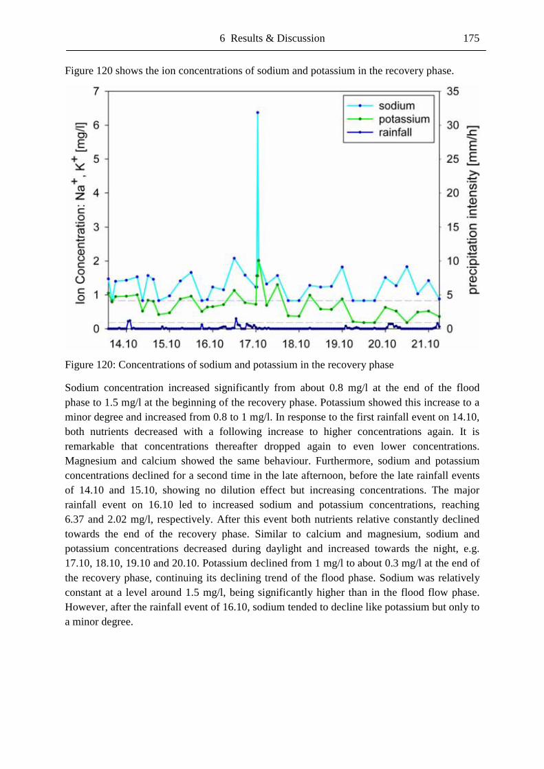
6 Results & Discussion 175

Figure 120 shows the ion concentrations of sodium and potassium in the recovery phase.

Figure 120: Concentrations of sodium and potassium in the recovery phase

Sodium concentration increased significantly from about 0.8 mg/l at the end of the flood phase to 1.5 mg/l at the beginning of the recovery phase. Potassium showed this increase to a minor degree and increased from 0.8 to 1 mg/l. In response to the first rainfall event on 14.10, both nutrients decreased with a following increase to higher concentrations again. It is remarkable that concentrations thereafter dropped again to even lower concentrations. Magnesium and calcium showed the same behaviour. Furthermore, sodium and potassium concentrations declined for a second time in the late afternoon, before the late rainfall events of 14.10 and 15.10, showing no dilution effect but increasing concentrations. The major rainfall event on 16.10 led to increased sodium and potassium concentrations, reaching 6.37 and 2.02 mg/l, respectively. After this event both nutrients relative constantly declined towards the end of the recovery phase. Similar to calcium and magnesium, sodium and potassium concentrations decreased during daylight and increased towards the night, e.g. 17.10, 18.10, 19.10 and 20.10. Potassium declined from 1 mg/l to about 0.3 mg/l at the end of the recovery phase, continuing its declining trend of the flood phase. Sodium was relatively constant at a level around 1.5 mg/l, being significantly higher than in the flood flow phase. However, after the rainfall event of 16.10, sodium tended to decline like potassium but only to a minor degree.

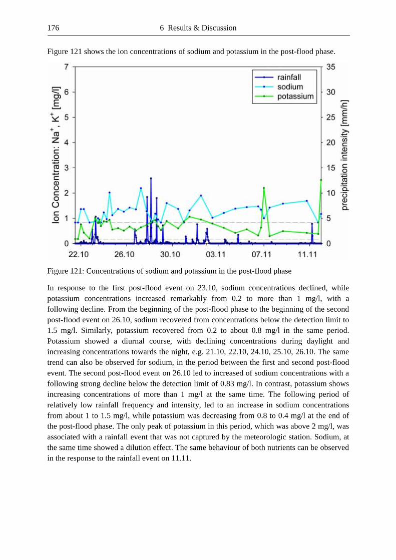
176 6 Results & Discussion

Figure 121 shows the ion concentrations of sodium and potassium in the post-flood phase.

Figure 121: Concentrations of sodium and potassium in the post-flood phase

In response to the first post-flood event on 23.10, sodium concentrations declined, while potassium concentrations increased remarkably from 0.2 to more than 1 mg/l, with a following decline. From the beginning of the post-flood phase to the beginning of the second post-flood event on 26.10, sodium recovered from concentrations below the detection limit to 1.5 mg/l. Similarly, potassium recovered from 0.2 to about 0.8 mg/l in the same period. Potassium showed a diurnal course, with declining concentrations during daylight and increasing concentrations towards the night, e.g. 21.10, 22.10, 24.10, 25.10, 26.10. The same trend can also be observed for sodium, in the period between the first and second post-flood event. The second post-flood event on 26.10 led to increased of sodium concentrations with a following strong decline below the detection limit of 0.83 mg/l. In contrast, potassium shows increasing concentrations of more than 1 mg/l at the same time. The following period of relatively low rainfall frequency and intensity, led to an increase in sodium concentrations from about 1 to 1.5 mg/l, while potassium was decreasing from 0.8 to 0.4 mg/l at the end of the post-flood phase. The only peak of potassium in this period, which was above 2 mg/l, was associated with a rainfall event that was not captured by the meteorologic station. Sodium, at the same time showed a dilution effect. The same behaviour of both nutrients can be observed in the response to the rainfall event on 11.11.

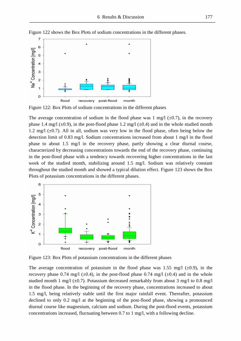
6 Results & Discussion 177

Figure 122 shows the Box Plots of sodium concentrations in the different phases.

Figure 122: Box Plots of sodium concentrations in the different phases

The average concentration of sodium in the flood phase was 1 mg/l (±0.7), in the recovery phase 1.4 mg/l (±0.9), in the post-flood phase 1.2 mg/l (±0.4) and in the whole studied month 1.2 mg/l (±0.7). All in all, sodium was very low in the flood phase, often being below the detection limit of 0.83 mg/l. Sodium concentrations increased from about 1 mg/l in the flood phase to about 1.5 mg/l in the recovery phase, partly showing a clear diurnal course, characterized by decreasing concentrations towards the end of the recovery phase, continuing in the post-flood phase with a tendency towards recovering higher concentrations in the last week of the studied month, stabilizing around 1.5 mg/l. Sodium was relatively constant throughout the studied month and showed a typical dilution effect. Figure 123 shows the Box Plots of potassium concentrations in the different phases.

Figure 123: Box Plots of potassium concentrations in the different phases

The average concentration of potassium in the flood phase was 1.55 mg/l (±0.9), in the recovery phase 0.74 mg/l (±0.4), in the post-flood phase 0.74 mg/l (±0.4) and in the whole studied month 1 mg/l (±0.7). Potassium decreased remarkably from about 3 mg/l to 0.8 mg/l in the flood phase. In the beginning of the recovery phase, concentrations increased to about 1.5 mg/l, being relatively stable until the first major rainfall event. Thereafter, potassium declined to only 0.2 mg/l at the beginning of the post-flood phase, showing a pronounced diurnal course like magnesium, calcium and sodium. During the post-flood events, potassium concentrations increased, fluctuating between 0.7 to 1 mg/l, with a following decline.

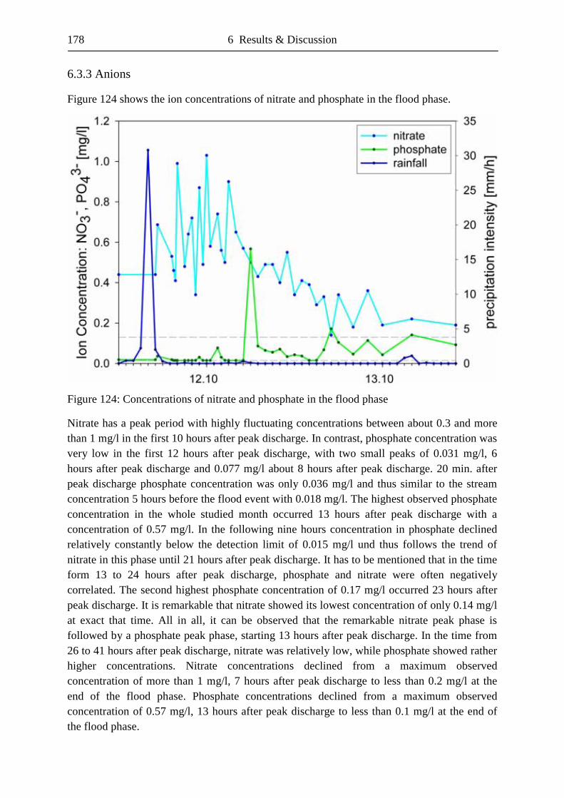
178 6 Results & Discussion

6.3.3 Anions Figure 124 shows the ion concentrations of nitrate and phosphate in the flood phase.

Figure 124: Concentrations of nitrate and phosphate in the flood phase

Nitrate has a peak period with highly fluctuating concentrations between about 0.3 and more than 1 mg/l in the first 10 hours after peak discharge. In contrast, phosphate concentration was very low in the first 12 hours after peak discharge, with two small peaks of 0.031 mg/l, 6 hours after peak discharge and 0.077 mg/l about 8 hours after peak discharge. 20 min. after peak discharge phosphate concentration was only 0.036 mg/l and thus similar to the stream concentration 5 hours before the flood event with 0.018 mg/l. The highest observed phosphate concentration in the whole studied month occurred 13 hours after peak discharge with a concentration of 0.57 mg/l. In the following nine hours concentration in phosphate declined relatively constantly below the detection limit of 0.015 mg/l und thus follows the trend of nitrate in this phase until 21 hours after peak discharge. It has to be mentioned that in the time form 13 to 24 hours after peak discharge, phosphate and nitrate were often negatively correlated. The second highest phosphate concentration of 0.17 mg/l occurred 23 hours after peak discharge. It is remarkable that nitrate showed its lowest concentration of only 0.14 mg/l at exact that time. All in all, it can be observed that the remarkable nitrate peak phase is followed by a phosphate peak phase, starting 13 hours after peak discharge. In the time from 26 to 41 hours after peak discharge, nitrate was relatively low, while phosphate showed rather higher concentrations. Nitrate concentrations declined from a maximum observed concentration of more than 1 mg/l, 7 hours after peak discharge to less than 0.2 mg/l at the end of the flood phase. Phosphate concentrations declined from a maximum observed concentration of 0.57 mg/l, 13 hours after peak discharge to less than 0.1 mg/l at the end of the flood phase.

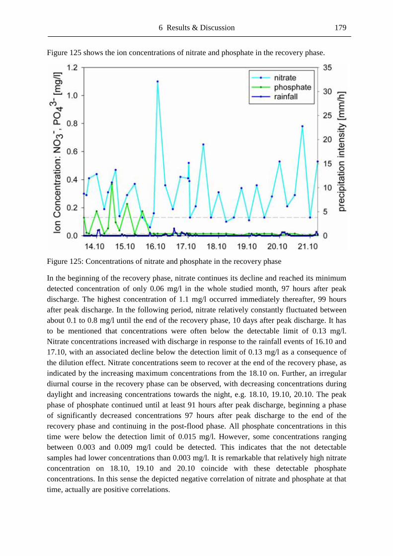
6 Results & Discussion 179

Figure 125 shows the ion concentrations of nitrate and phosphate in the recovery phase.

Figure 125: Concentrations of nitrate and phosphate in the recovery phase

In the beginning of the recovery phase, nitrate continues its decline and reached its minimum detected concentration of only 0.06 mg/l in the whole studied month, 97 hours after peak discharge. The highest concentration of 1.1 mg/l occurred immediately thereafter, 99 hours after peak discharge. In the following period, nitrate relatively constantly fluctuated between about 0.1 to 0.8 mg/l until the end of the recovery phase, 10 days after peak discharge. It has to be mentioned that concentrations were often below the detectable limit of 0.13 mg/l. Nitrate concentrations increased with discharge in response to the rainfall events of 16.10 and 17.10, with an associated decline below the detection limit of 0.13 mg/l as a consequence of the dilution effect. Nitrate concentrations seem to recover at the end of the recovery phase, as indicated by the increasing maximum concentrations from the 18.10 on. Further, an irregular diurnal course in the recovery phase can be observed, with decreasing concentrations during daylight and increasing concentrations towards the night, e.g. 18.10, 19.10, 20.10. The peak phase of phosphate continued until at least 91 hours after peak discharge, beginning a phase of significantly decreased concentrations 97 hours after peak discharge to the end of the recovery phase and continuing in the post-flood phase. All phosphate concentrations in this time were below the detection limit of 0.015 mg/l. However, some concentrations ranging between 0.003 and 0.009 mg/l could be detected. This indicates that the not detectable samples had lower concentrations than 0.003 mg/l. It is remarkable that relatively high nitrate concentration on 18.10, 19.10 and 20.10 coincide with these detectable phosphate concentrations. In this sense the depicted negative correlation of nitrate and phosphate at that time, actually are positive correlations.

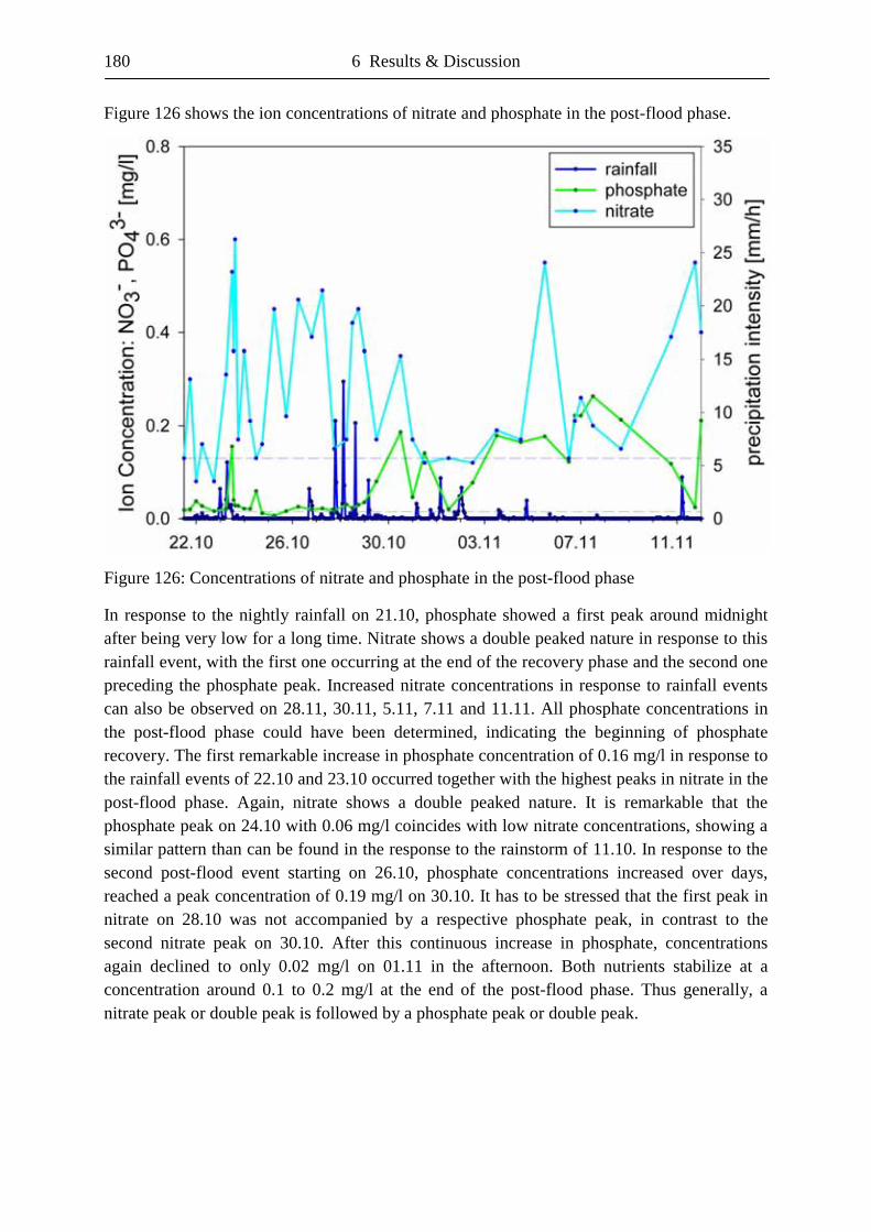
180 6 Results & Discussion

Figure 126 shows the ion concentrations of nitrate and phosphate in the post-flood phase.

Figure 126: Concentrations of nitrate and phosphate in the post-flood phase

In response to the nightly rainfall on 21.10, phosphate showed a first peak around midnight after being very low for a long time. Nitrate shows a double peaked nature in response to this rainfall event, with the first one occurring at the end of the recovery phase and the second one preceding the phosphate peak. Increased nitrate concentrations in response to rainfall events can also be observed on 28.11, 30.11, 5.11, 7.11 and 11.11. All phosphate concentrations in the post-flood phase could have been determined, indicating the beginning of phosphate recovery. The first remarkable increase in phosphate concentration of 0.16 mg/l in response to the rainfall events of 22.10 and 23.10 occurred together with the highest peaks in nitrate in the post-flood phase. Again, nitrate shows a double peaked nature. It is remarkable that the phosphate peak on 24.10 with 0.06 mg/l coincides with low nitrate concentrations, showing a similar pattern than can be found in the response to the rainstorm of 11.10. In response to the second post-flood event starting on 26.10, phosphate concentrations increased over days, reached a peak concentration of 0.19 mg/l on 30.10. It has to be stressed that the first peak in nitrate on 28.10 was not accompanied by a respective phosphate peak, in contrast to the second nitrate peak on 30.10. After this continuous increase in phosphate, concentrations again declined to only 0.02 mg/l on 01.11 in the afternoon. Both nutrients stabilize at a concentration around 0.1 to 0.2 mg/l at the end of the post-flood phase. Thus generally, a nitrate peak or double peak is followed by a phosphate peak or double peak.

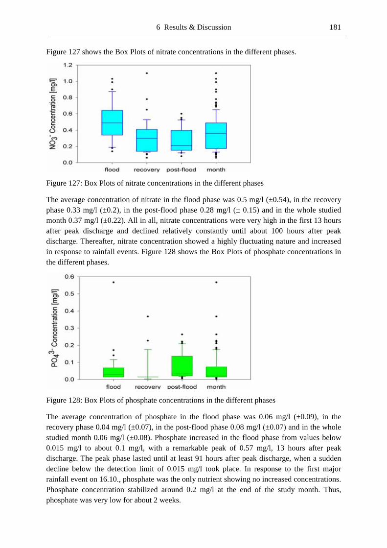
6 Results & Discussion 181

Figure 127 shows the Box Plots of nitrate concentrations in the different phases.

Figure 127: Box Plots of nitrate concentrations in the different phases

The average concentration of nitrate in the flood phase was 0.5 mg/l (±0.54), in the recovery phase 0.33 mg/l (±0.2), in the post-flood phase 0.28 mg/l (± 0.15) and in the whole studied month 0.37 mg/l (±0.22). All in all, nitrate concentrations were very high in the first 13 hours after peak discharge and declined relatively constantly until about 100 hours after peak discharge. Thereafter, nitrate concentration showed a highly fluctuating nature and increased in response to rainfall events. Figure 128 shows the Box Plots of phosphate concentrations in the different phases.

Figure 128: Box Plots of phosphate concentrations in the different phases

The average concentration of phosphate in the flood phase was 0.06 mg/l (±0.09), in the recovery phase 0.04 mg/l (±0.07), in the post-flood phase 0.08 mg/l (±0.07) and in the whole studied month 0.06 mg/l (±0.08). Phosphate increased in the flood phase from values below 0.015 mg/l to about 0.1 mg/l, with a remarkable peak of 0.57 mg/l, 13 hours after peak discharge. The peak phase lasted until at least 91 hours after peak discharge, when a sudden decline below the detection limit of 0.015 mg/l took place. In response to the first major rainfall event on 16.10., phosphate was the only nutrient showing no increased concentrations. Phosphate concentration stabilized around 0.2 mg/l at the end of the study month. Thus, phosphate was very low for about 2 weeks.

182 6 Results & Discussion

Figure 129 shows the ion concentrations of sulphate and chloride in the flood phase.

Figure 129: Concentrations of sulphate and chloride in the flood phase

Sulphate and chloride showed a very high average concentration of more than 4 mg/l and 3 mg/l, respectively, 20 minutes after peak discharge. 3 hours after peak discharge, sulphate and chloride showed a very high concentration of more than 9 mg/l and 3 mg/l, respectively. It has to be mentioned that all other nutrients, except for phosphate, also showed this second peak. After these peaks, sulphate showed constantly decreasing concentrations from about 1.4 mg/l to about 0.8 mg/l at the end of the flood phase, 41 hours after peak discharge. Chloride decreased from about 1.2 mg/l to 1 mg/l at the end of the flood phase. The lowest sulphate concentration occurred on 23 hours after peak discharge with 0.46 mg/l. At the same time chloride concentration was only 0.75 mg/l. Both nutrients are closely related and have about the same concentrations. Except for the two remarkable peaks, behaviour is completely different from that of phosphate and nitrate. Both nutrients are characterized by constantly low concentrations and tend to decrease to the end of the flood flow phase.

6 Results & Discussion 183

Figure 130 shows the ion concentrations of sulphate and chloride in the recovery phase.

Figure 130: Concentrations of sulphate and chloride in the recovery phase

Sulphate showed a significant rise from about 0.87 mg/l at the end of the flood phase to 1.26 mg/l in the beginning of the recovery phase. The same is true for chloride, increasing from 1.02 to 1.31 mg/l. In the evening of 14.10, both nutrients showed declining concentrations, sulphate from about 1.2 to 0.2 mg/l and chloride from about 1.2 to 0.9 mg/l. The same behaviour can be observed in the response to the rainfall event of 15.10. In response to the major rainfall event on 16.10 and 17.10, chloride concentration increased to 10.8 mg/l and sulphate concentration to 2.02 mg/l. Generally, a declining trend for both nutrients can be observed from about 1.2 mg/l at the beginning of the recovery phase to about 0.8 mg/l at the end of the recovery phase. It is remarkable that sulphate shows a pronounced diurnal course with declining concentrations during daylight and increasing concentrations towards the night that can be observed best on 14.10, 17 - 20.10 and 21 - 22.10. The chloride concentration follows this trend to a minor degree. Especially in the second half of the graph, a significant decline of both nutrients can be observed.

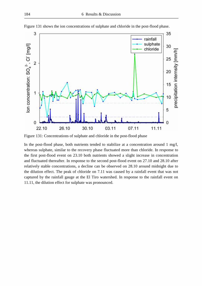
184 6 Results & Discussion

Figure 131 shows the ion concentrations of sulphate and chloride in the post-flood phase.

Figure 131: Concentrations of sulphate and chloride in the post-flood phase

In the post-flood phase, both nutrients tended to stabilize at a concentration around 1 mg/l, whereas sulphate, similar to the recovery phase fluctuated more than chloride. In response to the first post-flood event on 23.10 both nutrients showed a slight increase in concentration and fluctuated thereafter. In response to the second post-flood event on 27.10 and 28.10 after relatively stable concentrations, a decline can be observed on 28.10 around midnight due to the dilution effect. The peak of chloride on 7.11 was caused by a rainfall event that was not captured by the rainfall gauge at the El Tiro watershed. In response to the rainfall event on 11.11, the dilution effect for sulphate was pronounced.

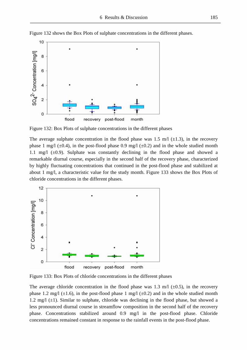
6 Results & Discussion 185

Figure 132 shows the Box Plots of sulphate concentrations in the different phases.

Figure 132: Box Plots of sulphate concentrations in the different phases

The average sulphate concentration in the flood phase was 1.5 m/l (±1.3), in the recovery phase 1 mg/l (±0.4), in the post-flood phase 0.9 mg/l (±0.2) and in the whole studied month 1.1 mg/l (±0.9). Sulphate was constantly declining in the flood phase and showed a remarkable diurnal course, especially in the second half of the recovery phase, characterized by highly fluctuating concentrations that continued in the post-flood phase and stabilized at about 1 mg/l, a characteristic value for the study month. Figure 133 shows the Box Plots of chloride concentrations in the different phases.

Figure 133: Box Plots of chloride concentrations in the different phases

The average chloride concentration in the flood phase was 1.3 m/l (±0.5), in the recovery phase 1.2 mg/l (±1.6), in the post-flood phase 1 mg/l (±0.2) and in the whole studied month 1.2 mg/l (±1). Similar to sulphate, chloride was declining in the flood phase, but showed a less pronounced diurnal course in streamflow composition in the second half of the recovery phase. Concentrations stabilized around 0.9 mg/l in the post-flood phase. Chloride concentrations remained constant in response to the rainfall events in the post-flood phase.

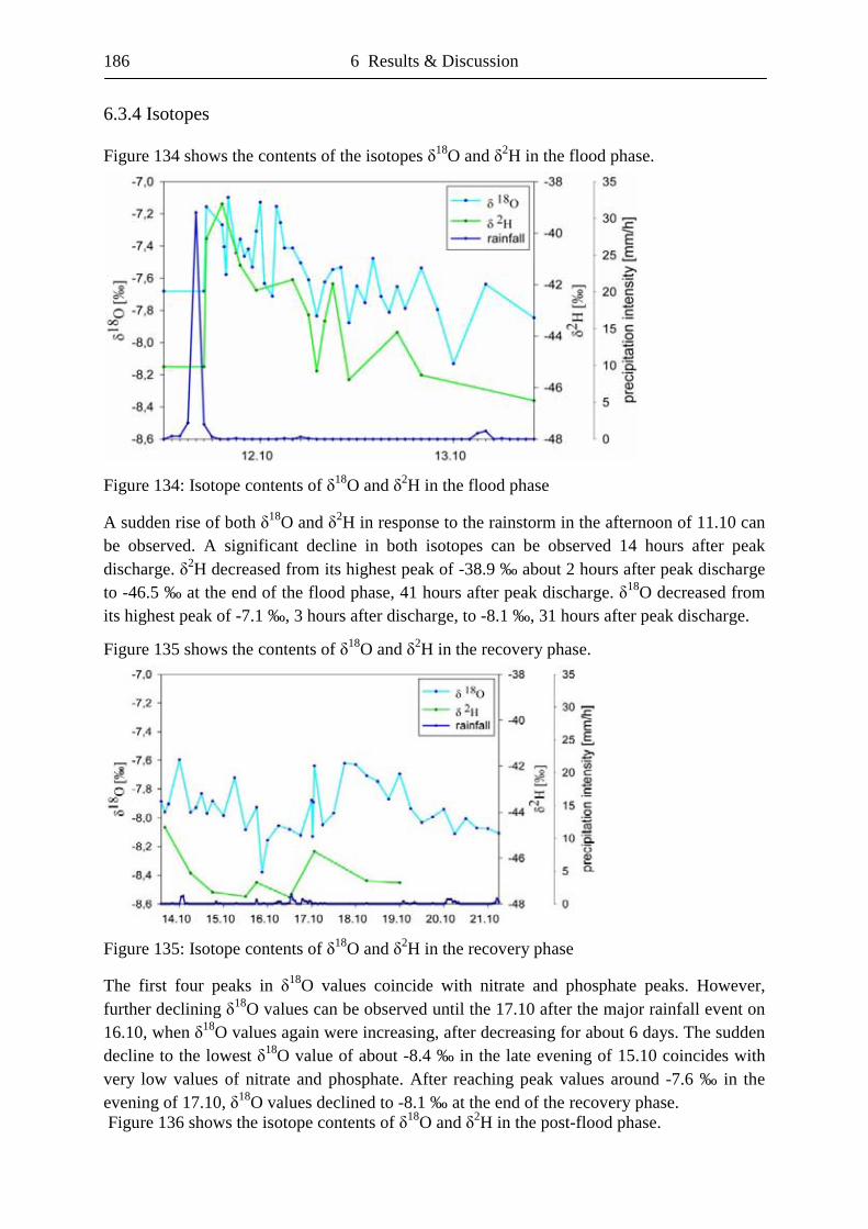
186 6 Results & Discussion

6.3.4 Isotopes Figure 134 shows the contents of the isotopes �18O and �2H in the flood phase.

Figure 134: Isotope contents of �18O and �2H in the flood phase

A sudden rise of both �18O and �2H in response to the rainstorm in the afternoon of 11.10 can be observed. A significant decline in both isotopes can be observed 14 hours after peak discharge. �2H decreased from its highest peak of -38.9 ‰ about 2 hours after peak discharge to -46.5 ‰ at the end of the flood phase, 41 hours after peak discharge. �18O decreased from its highest peak of -7.1 ‰, 3 hours after discharge, to -8.1 ‰, 31 hours after peak discharge. Figure 135 shows the contents of �18O and �2H in the recovery phase.

Figure 135: Isotope contents of �18O and �2H in the recovery phase

The first four peaks in �18O values coincide with nitrate and phosphate peaks. However, further declining �18O values can be observed until the 17.10 after the major rainfall event on 16.10, when �18O values again were increasing, after decreasing for about 6 days. The sudden decline to the lowest �18O value of about -8.4 ‰ in the late evening of 15.10 coincides with very low values of nitrate and phosphate. After reaching peak values around -7.6 ‰ in the evening of 17.10, �18O values declined to -8.1 ‰ at the end of the recovery phase. Figure 136 shows the isotope contents of �18O and �2H in the post-flood phase.

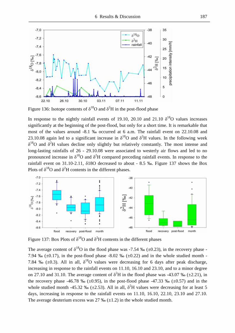
6 Results & Discussion 187

Figure 136: Isotope contents of �18O and �2H in the post-flood phase

In response to the nightly rainfall events of 19.10, 20.10 and 21.10 �18O values increases significantly at the beginning of the post-flood, but only for a short time. It is remarkable that most of the values around -8.1 ‰ occurred at 6 a.m. The rainfall event on 22.10.08 and 23.10.08 again led to a significant increase in �18O and �2H values. In the following week �18O and �2H values decline only slightly but relatively constantly. The most intense and long-lasting rainfalls of 26 - 29.10.08 were associated to westerly air flows and led to no pronounced increase in �18O and �2H compared preceding rainfall events. In response to the rainfall event on 31.10-2.11, �18O decreased to about - 8.5 ‰. Figure 137 shows the Box Plots of �18O and �2H contents in the different phases.

Figure 137: Box Plots of �18O and �2H contents in the different phases

The average content of �18O in the flood phase was -7.54 ‰ (±0.23), in the recovery phase -7.94 ‰ (±0.17), in the post-flood phase -8.02 ‰ (±0.22) and in the whole studied month -7.84 ‰ (±0.3). All in all, �18O values were decreasing for 6 days after peak discharge, increasing in response to the rainfall events on 11.10, 16.10 and 23.10, and to a minor degree on 27.10 and 31.10. The average content of �2H in the flood phase was -43.07 ‰ (±2.21), in the recovery phase -46.78 ‰ (±0.95), in the post-flood phase -47.33 ‰ (±0.57) and in the whole studied month -45.32 ‰ (±2.53). All in all, �2H values were decreasing for at least 5 days, increasing in response to the rainfall events on 11.10, 16.10, 22.10, 23.10 and 27.10. The average deuterium excess was 27 ‰ (±1.2) in the whole studied month.

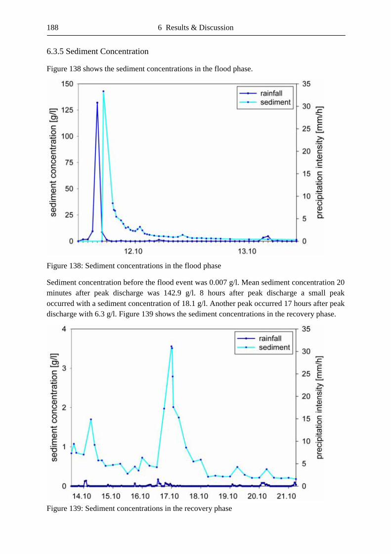
188 6 Results & Discussion

6.3.5 Sediment Concentration Figure 138 shows the sediment concentrations in the flood phase.

Figure 138: Sediment concentrations in the flood phase

Sediment concentration before the flood event was 0.007 g/l. Mean sediment concentration 20 minutes after peak discharge was 142.9 g/l. 8 hours after peak discharge a small peak occurred with a sediment concentration of 18.1 g/l. Another peak occurred 17 hours after peak discharge with 6.3 g/l. Figure 139 shows the sediment concentrations in the recovery phase.

Figure 139: Sediment concentrations in the recovery phase

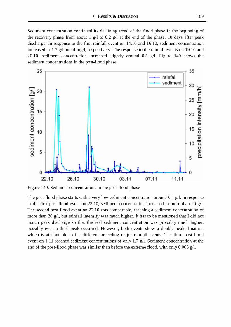
6 Results & Discussion 189

Sediment concentration continued its declining trend of the flood phase in the beginning of the recovery phase from about 1 g/l to 0.2 g/l at the end of the phase, 10 days after peak discharge. In response to the first rainfall event on 14.10 and 16.10, sediment concentration increased to 1.7 g/l and 4 mg/l, respectively. The response to the rainfall events on 19.10 and 20.10, sediment concentration increased slightly around 0.5 g/l. Figure 140 shows the sediment concentrations in the post-flood phase.

Figure 140: Sediment concentrations in the post-flood phase

The post-flood phase starts with a very low sediment concentration around 0.1 g/l. In response to the first post-flood event on 23.10, sediment concentration increased to more than 20 g/l. The second post-flood event on 27.10 was comparable, reaching a sediment concentration of more than 20 g/l, but rainfall intensity was much higher. It has to be mentioned that I did not match peak discharge so that the real sediment concentration was probably much higher, possibly even a third peak occurred. However, both events show a double peaked nature, which is attributable to the different preceding major rainfall events. The third post-flood event on 1.11 reached sediment concentrations of only 1.7 g/l. Sediment concentration at the end of the post-flood phase was similar than before the extreme flood, with only 0.006 g/l.

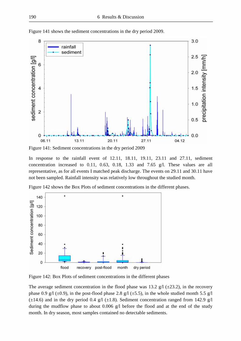
190 6 Results & Discussion

Figure 141 shows the sediment concentrations in the dry period 2009.

Figure 141: Sediment concentrations in the dry period 2009

In response to the rainfall event of 12.11, 18.11, 19.11, 23.11 and 27.11, sediment concentration increased to 0.11, 0.63, 0.18, 1.33 and 7.65 g/l. These values are all representative, as for all events I matched peak discharge. The events on 29.11 and 30.11 have not been sampled. Rainfall intensity was relatively low throughout the studied month. Figure 142 shows the Box Plots of sediment concentrations in the different phases.

Figure 142: Box Plots of sediment concentrations in the different phases

The average sediment concentration in the flood phase was 13.2 g/l (±23.2), in the recovery phase 0.9 g/l (±0.9), in the post-flood phase 2.8 g/l (±5.5), in the whole studied month 5.5 g/l (±14.6) and in the dry period 0.4 g/l (±1.8). Sediment concentration ranged from 142.9 g/l during the mudflow phase to about 0.006 g/l before the flood and at the end of the study month. In dry season, most samples contained no detectable sediments.

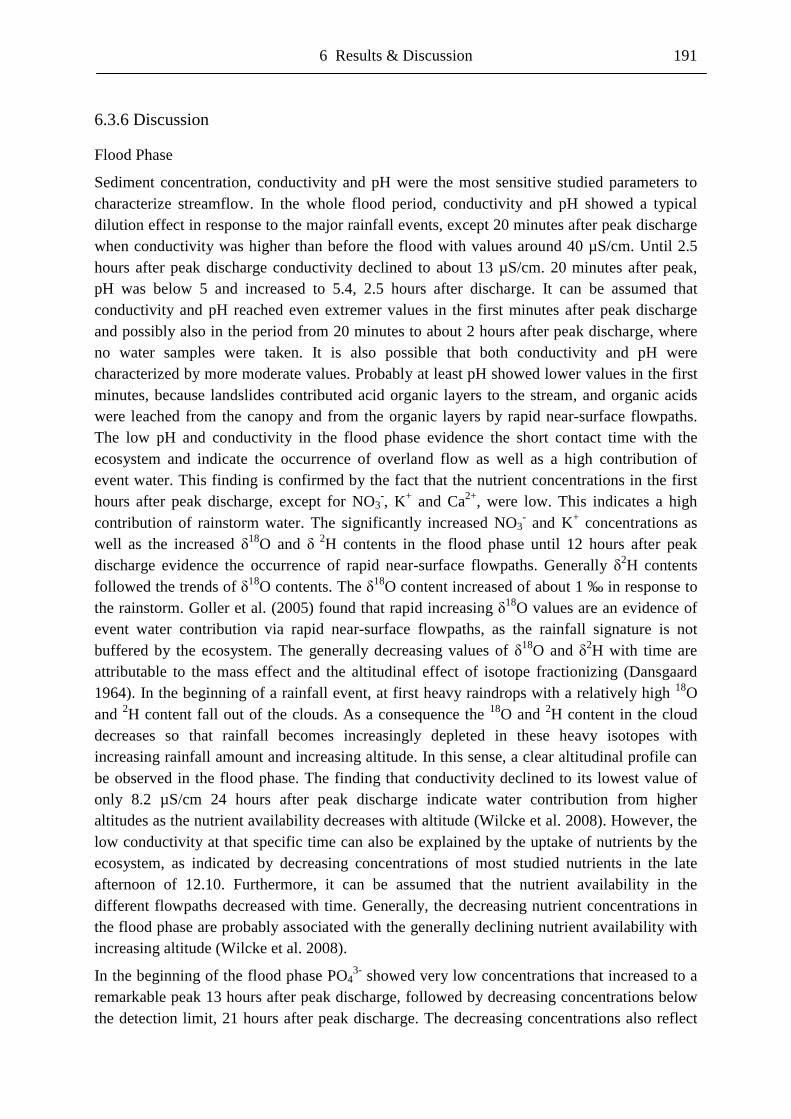
6 Results & Discussion 191

6.3.6 Discussion Flood Phase

Sediment concentration, conductivity and pH were the most sensitive studied parameters to characterize streamflow. In the whole flood period, conductivity and pH showed a typical dilution effect in response to the major rainfall events, except 20 minutes after peak discharge when conductivity was higher than before the flood with values around 40 µS/cm. Until 2.5 hours after peak discharge conductivity declined to about 13 µS/cm. 20 minutes after peak, pH was below 5 and increased to 5.4, 2.5 hours after discharge. It can be assumed that conductivity and pH reached even extremer values in the first minutes after peak discharge and possibly also in the period from 20 minutes to about 2 hours after peak discharge, where no water samples were taken. It is also possible that both conductivity and pH were characterized by more moderate values. Probably at least pH showed lower values in the first minutes, because landslides contributed acid organic layers to the stream, and organic acids were leached from the canopy and from the organic layers by rapid near-surface flowpaths. The low pH and conductivity in the flood phase evidence the short contact time with the ecosystem and indicate the occurrence of overland flow as well as a high contribution of event water. This finding is confirmed by the fact that the nutrient concentrations in the first hours after peak discharge, except for NO3

-, K+ and Ca2+, were low. This indicates a high contribution of rainstorm water. The significantly increased NO3

- and K+ concentrations as well as the increased �18O and � 2H contents in the flood phase until 12 hours after peak discharge evidence the occurrence of rapid near-surface flowpaths. Generally �2H contents followed the trends of �18O contents. The �18O content increased of about 1 ‰ in response to the rainstorm. Goller et al. (2005) found that rapid increasing �18O values are an evidence of event water contribution via rapid near-surface flowpaths, as the rainfall signature is not buffered by the ecosystem. The generally decreasing values of �18O and �2H with time are attributable to the mass effect and the altitudinal effect of isotope fractionizing (Dansgaard 1964). In the beginning of a rainfall event, at first heavy raindrops with a relatively high 18O and 2H content fall out of the clouds. As a consequence the 18O and 2H content in the cloud decreases so that rainfall becomes increasingly depleted in these heavy isotopes with increasing rainfall amount and increasing altitude. In this sense, a clear altitudinal profile can be observed in the flood phase. The finding that conductivity declined to its lowest value of only 8.2 µS/cm 24 hours after peak discharge indicate water contribution from higher altitudes as the nutrient availability decreases with altitude (Wilcke et al. 2008). However, the low conductivity at that specific time can also be explained by the uptake of nutrients by the ecosystem, as indicated by decreasing concentrations of most studied nutrients in the late afternoon of 12.10. Furthermore, it can be assumed that the nutrient availability in the different flowpaths decreased with time. Generally, the decreasing nutrient concentrations in the flood phase are probably associated with the generally declining nutrient availability with increasing altitude (Wilcke et al. 2008).

In the beginning of the flood phase PO43- showed very low concentrations that increased to a

remarkable peak 13 hours after peak discharge, followed by decreasing concentrations below the detection limit, 21 hours after peak discharge. The decreasing concentrations also reflect

192 6 Results & Discussion

the decreasing nutrient availability with altitude (Wilcke et al. 2008). This assumption is confirmed by the decreasing NO3

- concentrations from 13 hours to 23 hours after peak discharge. NO3

- reached its lowest concentration at the same time when PO43- showed a

second remarkable peak 23 hours after peak discharge. Together with the further declining �18O values in this period, water contribution from higher altitudes is obvious. Further, a general feature of water chemistry in response to the rainstorm and following rainfall events was that the peak in NO3

- was followed by a peak in PO43-. This behaviour can be explained

by the decreasing N availability with increasing altitude (Wilcke et al. 2008). Thus, if there is a plant growth limiting nutrient, probably NO3

- is the candidate in higher altitudes and PO43-

in lower altitudes of the San Francisco Valley. It is striking that PO43- concentrations

increased significantly 23 hours after peak discharge, when all other nutrients showed significantly declined concentrations. This indicates that there is a surplus of PO4

3- in a certain altitude which might be the transition zone between 2600 - 2800 m, where atmospheric inputs of PO4

3- are especially high (Rollenbeck et al. 2008). However, it seems that PO43- is

decoupled from the general trends in nutrient cycling, although from 24 hours after peak discharge to the end of the flood phase NO3

- and PO43- were closely related.

The highly fluctuating Ca2+ concentrations probably derive from the numerous erosional and depositional landforms, most notably the deep reaching landslides along the river channel and the new formed terraces. While the lower concentrations represent the signature of pure rainfall composition and thus the short contact time with the ecosystem, the higher concentrations represent the erosional force of the destructive debris flow flood wave and possibly also old water contribution. In this sense the fluctuating Ca2+ concentrations reflect the different altitudes and distances of erosional and depositional features to the sample location nearby the ECSF. K+ showed generally high and constantly decreasing concentrations in the first 10 hours after peak discharge with four peaks. These peaks might be associated to overland flow and thus should reflect differently distant areas of the drainage basin to the sample location. It has to be mentioned that while all nutrients showed peak concentrations 3 hours after peak discharge K+ showed a double peaked nature, with the first peak occurring half an hour earlier than the main peak reflected by all other nutrients, except for PO4

3-. This can be explained by the fact that K+ is mainly supplied by the rapid overland flow. Na+ and K+ showed slightly decreasing concentrations in the end of the flood phase. This indicates that both nutrients have been hold back by the ecosystem, after the significant losses, especially of K+ in the beginning of the flood phase. Probably K+ concentrations were very high in the first two hours after peak discharge due to the occurrence of overland flow and leaching processes from the canopy. Na+, K+, Mg2+ and partly also Ca2+ showed slightly increasing concentrations from 13 to 21 hours after peak discharge. SO4

2- and Cl- concentrations also decreased in the flood phase. As the concentrations of all nutrients in the water sample taken 3 hours after discharge were significantly higher than in rainwater, this sample probably represents a late pre-event water contribution. A possible uptake by the ecosystem in the flood phase can be observed for NO3

-, Ca2+, Mg2+, SO42-, Cl-, K+ and Na+, all

showing very low or concentrations below the detection limit from 22 - 24 hours after peak discharge during daylight from 3 to 5 p.m. Taking into account the typical response time of the drainage basin of 3 to 6 hours, this time of the day reflects the water composition of the period of maximum evapotranspiration around noon.

6 Results & Discussion 193

Recovery Phase

The decreasing �18O and �2H contents as well as the decreasing K+, NO3- and PO4

3- concentrations until the late evening of 15.10 seem to mark the end of water contribution from the rainstorm of 11.10. The similar low �18O contents on 16.10 and 17.10 indicate that water contribution around this time also originated from the rainstorm. Taking this assumption into account, then the rainfall event on 16.10 triggered the final contribution of the now one week old pre-event water of the rainstorm at midnight of the 17.10. Thus, the rainstorm water influenced streamflow composition and remained in the ecosystem for about one week. The rainfall event of 16.10 first led to an enrichment of �18O and �2H contents, reflecting fast near-surface lateral flowpaths and in the following hours and days to a depletion of �18O and �2H contents, reflecting the altitudinal and mass effect of isotope fractionizing. The residence time of this water, with a peak about six hours after rainfall and a more pronounced long-lasting peak that started in the late evening of 17.10 demonstrate the slow and long lasting response of the catchment to low intensity rainfalls. Furthermore, �18O contents declined until the end of the recovery phase, indicating a long residence time that seems to be associated with the low intensity rainfall event. Generally, the increasing pH and conductivity values throughout the recovery phase indicate that the impact of the rainstorm lasted for at least 10 days.

The sudden rise of conductivity in the beginning of the recovery phase and the constantly increasing pH indicate that water with a longer contact time and thus slower flowpaths reached the ECSF about 46 hours after peak discharge. In response to the rainfall event on 16.10 only a relatively weak dilution effect could be observed, probably due to the relatively long residence time of the low intensity rainfall event. Thus, the ecosystem buffered the pure chemical rainfall signature. Probably this rainfall event also contributed pre-event water of the rainstorm on 11.10 to the streams, as indicated by the low �18O contents. The rapid increasing pH values after this event might be associated with the washout of nutrients from the new formed terraces in the river channel and/or pre-event water contribution, as also indicated by increasing conductivity values.

NO3-, Cl-, SO4

2-, Na+, K+, Mg2+ and Ca2+ showed significantly increased concentrations in response to the rainfall event on 16.10, while PO4

3- remained below the detection limit. Thus the nutrient availability was very high. Possible reasons might be decomposition and mineralization processes of organic and inorganic materials supplied by wash-out and leaching processes from new formed or affected erosional and depositional landforms such as terraces, landslides and gullies. These major nutrient contributing features can be assumed to be most effective in the Rio San Francisco channel itself. The contribution of the now 5 days old water of the rainstorm event of 11.10 also might have contributed to the increased nutrient concentrations. However, the sharp peaks that were associated with a rising discharge stage indicate that a large proportion of the exported nutrients were provided by the river channel and the slopes of terraces. This assumption is based on the fact that the river channel was flooded for the first time after the rainstorm event of 11.10. The observation that PO4

3- was the only nutrient that showed no increased concentrations to the rainfall event on 16.10 indicates that PO4

3- was even hold back within the new formed erosional and depositional landforms in the river channel.

194 6 Results & Discussion

In the recovery phase, NO3- reached its lowest concentration at about the same time when

PO43- started its minimum phase that lasted at least to the end of the recovery phase, 10 days

after peak discharge. Immediately thereafter, NO3- reached its highest concentration in

response to the rainfall event of 16.10. It is striking that this NO3- peak was not followed by a

PO43- peak, indicating the beginning of retardation of PO4

3- by the ecosystem. NO3- showed

highly fluctuating concentrations that mainly declined during daylight and in the late evening, and increased toward the night in the period from 16.10 - 27.10. This diurnal course is also reflected by SO4

2- from 17.10 - 25.10 in a more constant and pronounced way. Cl-, generally following the trends of SO4

2- throughout the studied month showed this diurnal course only to a minor degree. Ca2+ showed decreasing concentrations during daylight on 13.10, 14.10, 15.10 and 17.10 - 23.10. Mg2+ showed decreasing concentrations during daylight on 13.10, 14.10 and 17.10 - 28.10. K + showed decreasing concentrations during daylight on 12.10 - 14.10 and 17.10 - 26.10. Na+ seems to be effected by nutrient retardation by the ecosystem only in a minor degree, but generally follows the diurnal course of K+. All in all, in the recovery phase most of the major nutrients were hold back by the ecosystem in response to the high nutrient losses caused by the rainstorm of 11.10. PO4

3-, SO42-, Cl- and K+ showed

continuously decreasing concentrations in the recovery phase, while pH and conductivity increased relatively continuously. Especially K+ was significantly declining over weeks, reflecting the immense loss due to leaching processes and overland flow during the flood phase. The diurnal course of most studied nutrients indicate, that the major impact time of the extreme flood on the nutrient cycle of the ecosystem and thus on streamflow composition lasted for at least 10 days to the end of the recovery phase. Post-Flood Phase

The low PO43- concentrations and the continuing diurnal course of NO3

-, K+ and Mg2+ indicate that the total impact time of the rainstorm on the nutrient cycle lasted for at least 17 days until the 28.10. K+ showed increased concentrations in response to the three major rainfall events in the post-flood phase, indicating rapid near-surface flowpaths and leaching processes from the canopy and the organic layers. After each rainfall event, K+ was most probably retained by the ecosystem, as indicated by the constantly declining K+ concentration not only after rainfall events, but also during the relatively dry period at the end of the post-flood phase. Na+ showed no reaction to the first post-flood event, decreasing concentrations during the second-post flood event and increasing concentrations in response to the third post-flood event. In response to the rainfall event on 06.11 and 11.11, K+ concentrations increased, while Na+ concentrations decreased, showing a typical dilution effect. In response to the first post-flood event Ca2+ and Mg2+ showed increased concentrations. Probably these high concentrations derived from wash-out processes from the new erosional and depositional landforms in the river channel most notably from the new formed terraces that were flooded for the first time after the extreme flood. This assumption is supported by the rather decreasing concentrations of both nutrients during the second post-flood event. However, the dilution effect through nutrient-poor rainfall probably also contributed to the decreased concentrations. The isolated short but remarkable Ca2+ peak indicates that the second-post flood event might have overtopped the stage of the first-post flood event in some locations. In response to the third-post flood event, both nutrients showed rather increased concentrations,

6 Results & Discussion 195

likewise in response to the rainfall event 6.11. In contrast, Ca2+ and Mg2+ declined in response to the rainfall event of 11.11, showing a typical dilution effect.

In response to the rainfall event on 23.10, both NO3- and PO4

3- increased. PO43- showed its

first remarkable peak after being below the detection limit for about 6 days, again occurring after the NO3

- peak. It is remarkable that the second PO43- peak coincided with a very low not

detectable NO3- concentration. This behaviour of streamflow composition was similar to the

response pattern to the rainstorm of 11.10, indicating that the water originated from higher altitudes, where N availability is lower than P availability. In response to the second post-flood event, NO3

- showed two remarkable peaks, with the second one being accompanied with a remarkable PO4

3- peak. Thereafter another PO43- peak followed. Thus, similar to the

response to the rainstorm and the first post-flood event, the NO3- peak was followed by a

PO43- peak. Cl- and SO4

2- showed no significant changes in their concentrations in response to the first, second and third post-flood event. All in all, PO4

3- was hold back by the ecosystem for at least two weeks and probably even for three weeks. In the post-flood phase, PO4

3- experienced leaching processes during the first and second post-flood events that were probably limited to higher altitudes, as indicated by the delayed response compared to NO3

-. The first increase in PO4

3- concentration in response to the first post-flood event is most probably linked with wash-out processes in the river channel, especially from the terraces that were flooded for the first time after the extreme flood of 11.10.

It can be assumed that the rainfall events between 26.10 and 03.11 that originated from coastal regions had lower �18O and �2H contents than the preceding easterly airflows as indicated by the decline of �18O contents throughout the post-flood phase. The rising �18O contents from 06.11 to the end of the study period are linked with easterly air flow and thus confirm this assumption of different composition in isotope contents in respect of the origin of the respective air masses. However, as the �18O contents of both sources are similar and westerly airflows frequently influenced easterly airflows, as indicated by the numerous nightly rainfalls a separation between the two becomes complicated. All in all, a quite good correlation of rising isotope contents in response to the major rainfall events and following declining isotope contents as a consequence of the altitudinal and mass effect can be observed (Dansgaard 1964). The rapid increase in isotope content evidences the occurrence of near-surface lateral flowpaths as the rainfall signature was not buffered by the ecosystem. Dry Period

In the dry period, which is represented by the first sampled two weeks, conductivity was significantly higher than in the post-flood phase. The same is true for pH that had a characteristic value of about 8. The increase in pH in response to the rainfall event on 15.11 and 18.11 to 8.4 and to 9, respectively, evidences pre-event water contribution. Generally, the high values in both pH and conductivity reflect the long residence time within the ecosystem. However, in response to the rainfall events on 12.11, 21 - 24.11, 26 - 27.11 and 29.11 a typical dilution effect could be observed. Thus also event water contribution could be observed. Generally, the dry period demonstrates the problematic separation of old and new water contribution due to the occurrence of multiple populations, which means that two different sources of water become mixed. The rhythmic hourly pattern of fluctuating high and

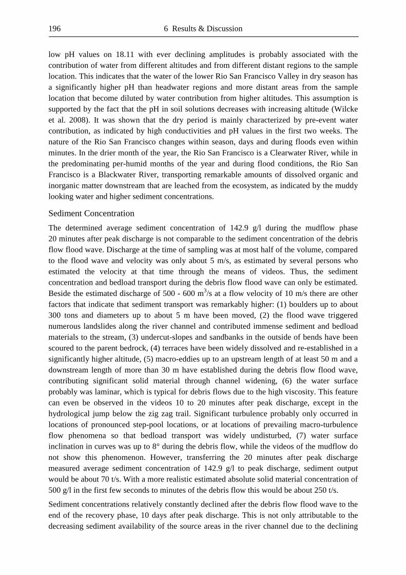
196 6 Results & Discussion

low pH values on 18.11 with ever declining amplitudes is probably associated with the contribution of water from different altitudes and from different distant regions to the sample location. This indicates that the water of the lower Rio San Francisco Valley in dry season has a significantly higher pH than headwater regions and more distant areas from the sample location that become diluted by water contribution from higher altitudes. This assumption is supported by the fact that the pH in soil solutions decreases with increasing altitude (Wilcke et al. 2008). It was shown that the dry period is mainly characterized by pre-event water contribution, as indicated by high conductivities and pH values in the first two weeks. The nature of the Rio San Francisco changes within season, days and during floods even within minutes. In the drier month of the year, the Rio San Francisco is a Clearwater River, while in the predominating per-humid months of the year and during flood conditions, the Rio San Francisco is a Blackwater River, transporting remarkable amounts of dissolved organic and inorganic matter downstream that are leached from the ecosystem, as indicated by the muddy looking water and higher sediment concentrations.

Sediment Concentration

The determined average sediment concentration of 142.9 g/l during the mudflow phase 20 minutes after peak discharge is not comparable to the sediment concentration of the debris flow flood wave. Discharge at the time of sampling was at most half of the volume, compared to the flood wave and velocity was only about 5 m/s, as estimated by several persons who estimated the velocity at that time through the means of videos. Thus, the sediment concentration and bedload transport during the debris flow flood wave can only be estimated. Beside the estimated discharge of 500 - 600 m3/s at a flow velocity of 10 m/s there are other factors that indicate that sediment transport was remarkably higher: (1) boulders up to about 300 tons and diameters up to about 5 m have been moved, (2) the flood wave triggered numerous landslides along the river channel and contributed immense sediment and bedload materials to the stream, (3) undercut-slopes and sandbanks in the outside of bends have been scoured to the parent bedrock, (4) terraces have been widely dissolved and re-established in a significantly higher altitude, (5) macro-eddies up to an upstream length of at least 50 m and a downstream length of more than 30 m have established during the debris flow flood wave, contributing significant solid material through channel widening, (6) the water surface probably was laminar, which is typical for debris flows due to the high viscosity. This feature can even be observed in the videos 10 to 20 minutes after peak discharge, except in the hydrological jump below the zig zag trail. Significant turbulence probably only occurred in locations of pronounced step-pool locations, or at locations of prevailing macro-turbulence flow phenomena so that bedload transport was widely undisturbed, (7) water surface inclination in curves was up to 8° during the debris flow, while the videos of the mudflow do not show this phenomenon. However, transferring the 20 minutes after peak discharge measured average sediment concentration of 142.9 g/l to peak discharge, sediment output would be about 70 t/s. With a more realistic estimated absolute solid material concentration of 500 g/l in the first few seconds to minutes of the debris flow this would be about 250 t/s.

Sediment concentrations relatively constantly declined after the debris flow flood wave to the end of the recovery phase, 10 days after peak discharge. This is not only attributable to the decreasing sediment availability of the source areas in the river channel due to the declining

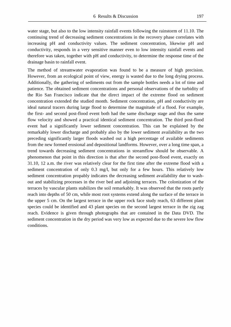
6 Results & Discussion 197

water stage, but also to the low intensity rainfall events following the rainstorm of 11.10. The continuing trend of decreasing sediment concentrations in the recovery phase correlates with increasing pH and conductivity values. The sediment concentration, likewise pH and conductivity, responds in a very sensitive manner even to low intensity rainfall events and therefore was taken, together with pH and conductivity, to determine the response time of the drainage basin to rainfall event.

The method of streamwater evaporation was found to be a measure of high precision. However, from an ecological point of view, energy is wasted due to the long drying process. Additionally, the gathering of sediments out from the sample bottles needs a lot of time and patience. The obtained sediment concentrations and personal observations of the turbidity of the Rio San Francisco indicate that the direct impact of the extreme flood on sediment concentration extended the studied month. Sediment concentration, pH and conductivity are ideal natural tracers during large flood to determine the magnitude of a flood. For example, the first- and second post-flood event both had the same discharge stage and thus the same flow velocity and showed a practical identical sediment concentration. The third post-flood event had a significantly lower sediment concentration. This can be explained by the remarkably lower discharge and probably also by the lower sediment availability as the two preceding significantly larger floods washed out a high percentage of available sediments from the new formed erosional and depositional landforms. However, over a long time span, a trend towards decreasing sediment concentrations in streamflow should be observable. A phenomenon that point in this direction is that after the second post-flood event, exactly on 31.10, 12 a.m. the river was relatively clear for the first time after the extreme flood with a sediment concentration of only 0.3 mg/l, but only for a few hours. This relatively low sediment concentration propably indicates the decreasing sediment availability due to wash-out and stabilizing processes in the river bed and adjoining terraces. The colonization of the terraces by vascular plants stabilizes the soil remarkably. It was observed that the roots partly reach into depths of 50 cm, while most root systems extend along the surface of the terrace in the upper 5 cm. On the largest terrace in the upper rock face study reach, 63 different plant species could be identified and 43 plant species on the second largest terrace in the zig zag reach. Evidence is given through photographs that are contained in the Data DVD. The sediment concentration in the dry period was very low as expected due to the severe low flow conditions.

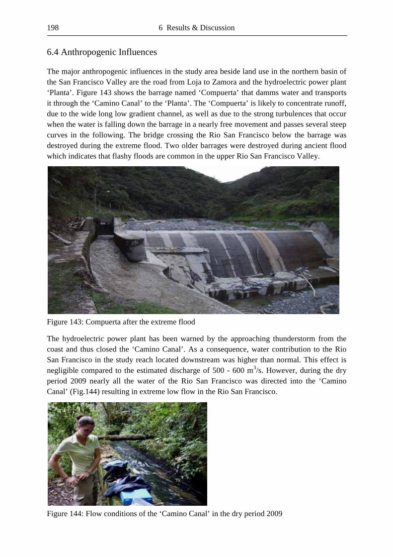
198 6 Results & Discussion

6.4 Anthropogenic Influences

The major anthropogenic influences in the study area beside land use in the northern basin of the San Francisco Valley are the road from Loja to Zamora and the hydroelectric power plant ‘Planta’. Figure 143 shows the barrage named ‘Compuerta’ that damms water and transports it through the ‘Camino Canal’ to the ‘Planta’. The ‘Compuerta’ is likely to concentrate runoff, due to the wide long low gradient channel, as well as due to the strong turbulences that occur when the water is falling down the barrage in a nearly free movement and passes several steep curves in the following. The bridge crossing the Rio San Francisco below the barrage was destroyed during the extreme flood. Two older barrages were destroyed during ancient flood which indicates that flashy floods are common in the upper Rio San Francisco Valley.

Figure 143: Compuerta after the extreme flood

The hydroelectric power plant has been warned by the approaching thunderstorm from the coast and thus closed the ‘Camino Canal’. As a consequence, water contribution to the Rio San Francisco in the study reach located downstream was higher than normal. This effect is negligible compared to the estimated discharge of 500 - 600 m3/s. However, during the dry period 2009 nearly all the water of the Rio San Francisco was directed into the ‘Camino Canal’ (Fig.144) resulting in extreme low flow in the Rio San Francisco.

Figure 144: Flow conditions of the ‘Camino Canal’ in the dry period 2009

6 Results & Discussion 199

Discharge in the ‘Camino Canal’ was estimated to be at least 1 m3/s at a flow velocity around 3 m/s. This not seems to be a high value, but when considering that not all of this water, bypassing the Rio San Francisco, was actually used for power generation, it becomes meaningful. Surplus water was directed into ‘Quebrada Milagro’, a cascade near the ‘Planta’. The influence of the hydroelectric power plant becomes clear by a comparison of the discharge of the ‘Camino Canal’ and the affected reach of the Rio San Francisco (Fig.145).

Figure 145: Extreme low flow conditions in the Rio San Francisco from the ‘Compuerta’ to the tributary immediately upstream of the tara bita rock face

The very low discharge of the Rio San Francisco in the dry period November 2009 can be identified in the upper left region of the picture. The tributary originating from the ‘Pastos’ carried many times more water than the major Rio San Francisco. Due to the immense differences in flow velocity between pools and riffles during such low flow conditions, the simplest hydrologic method to determine discharge was used, the bucket method. Thereby a confined riffle or step location is used to direct the streamflow for one second into a bucket of commonly 10 l volume. Discharge was estimated on 5.11 and 6.11, with each ten measurement of one second at the location given in Figure 138, to be 5 l/s (±0.2) and 4.6 l/s (±0.2), respectively at a conductivity of 33 µS/cm and 37 µS/cm and a pH of 8.3 and 7.8, respectively. On 15.11, 21.11 and 3.12, discharge was estimated 50 m further upstream to be 7.4 l/s (±0.3), 7.8 l/s (±0.2) and 4 l/s (±0.3), respectively at a conductivity of 34 µS/cm, 35 µS/cm and 35 µS/cm and a pH of 8.4, 7.8 and 7.6, respectively. The average discharge of the five days of measurement was 5.8 l/s (±1.5). Thus, discharge during the extreme flood in October 2008 was about 100.000 times higher than during the dry period in November 2009 in the study reach located between the ‘Compuerta’ and the ‘Planta’. This extreme difference was only possible due to the outtake of water by the hydroelectric power plant. Without the water outtake of the hydroelectric power plant, discharge would have been ‘only’ about 500 times higher during the extreme flood, compared to the dry period.

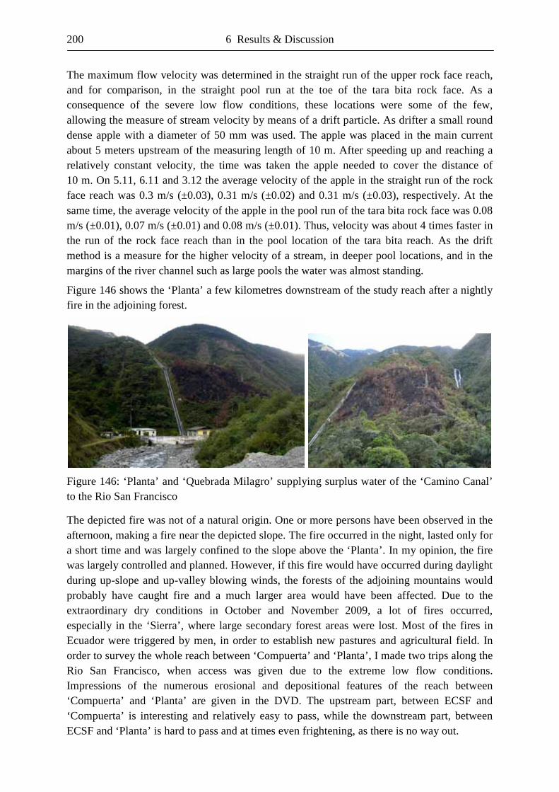
200 6 Results & Discussion

The maximum flow velocity was determined in the straight run of the upper rock face reach, and for comparison, in the straight pool run at the toe of the tara bita rock face. As a consequence of the severe low flow conditions, these locations were some of the few, allowing the measure of stream velocity by means of a drift particle. As drifter a small round dense apple with a diameter of 50 mm was used. The apple was placed in the main current about 5 meters upstream of the measuring length of 10 m. After speeding up and reaching a relatively constant velocity, the time was taken the apple needed to cover the distance of 10 m. On 5.11, 6.11 and 3.12 the average velocity of the apple in the straight run of the rock face reach was 0.3 m/s (±0.03), 0.31 m/s (±0.02) and 0.31 m/s (±0.03), respectively. At the same time, the average velocity of the apple in the pool run of the tara bita rock face was 0.08 m/s (±0.01), 0.07 m/s (±0.01) and 0.08 m/s (±0.01). Thus, velocity was about 4 times faster in the run of the rock face reach than in the pool location of the tara bita reach. As the drift method is a measure for the higher velocity of a stream, in deeper pool locations, and in the margins of the river channel such as large pools the water was almost standing.

Figure 146 shows the ‘Planta’ a few kilometres downstream of the study reach after a nightly fire in the adjoining forest.

Figure 146: ‘Planta’ and ‘Quebrada Milagro’ supplying surplus water of the ‘Camino Canal’ to the Rio San Francisco

The depicted fire was not of a natural origin. One or more persons have been observed in the afternoon, making a fire near the depicted slope. The fire occurred in the night, lasted only for a short time and was largely confined to the slope above the ‘Planta’. In my opinion, the fire was largely controlled and planned. However, if this fire would have occurred during daylight during up-slope and up-valley blowing winds, the forests of the adjoining mountains would probably have caught fire and a much larger area would have been affected. Due to the extraordinary dry conditions in October and November 2009, a lot of fires occurred, especially in the ‘Sierra’, where large secondary forest areas were lost. Most of the fires in Ecuador were triggered by men, in order to establish new pastures and agricultural field. In order to survey the whole reach between ‘Compuerta’ and ‘Planta’, I made two trips along the Rio San Francisco, when access was given due to the extreme low flow conditions. Impressions of the numerous erosional and depositional features of the reach between ‘Compuerta’ and ‘Planta’ are given in the DVD. The upstream part, between ECSF and ‘Compuerta’ is interesting and relatively easy to pass, while the downstream part, between ECSF and ‘Planta’ is hard to pass and at times even frightening, as there is no way out.

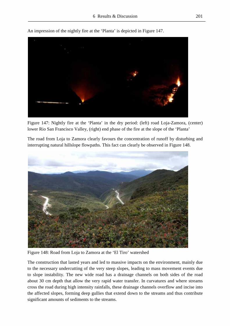
6 Results & Discussion 201

An impression of the nightly fire at the ‘Planta’ is depicted in Figure 147.

Figure 147: Nightly fire at the ‘Planta’ in the dry period: (left) road Loja-Zamora, (center) lower Rio San Francisco Valley, (right) end phase of the fire at the slope of the ‘Planta’

The road from Loja to Zamora clearly favours the concentration of runoff by disturbing and interrupting natural hillslope flowpaths. This fact can clearly be observed in Figure 148.

Figure 148: Road from Loja to Zamora at the ‘El Tiro’ watershed

The construction that lasted years and led to massive impacts on the environment, mainly due to the necessary undercutting of the very steep slopes, leading to mass movement events due to slope instability. The new wide road has a drainage channels on both sides of the road about 30 cm depth that allow the very rapid water transfer. In curvatures and where streams cross the road during high intensity rainfalls, these drainage channels overflow and incise into the affected slopes, forming deep gullies that extend down to the streams and thus contribute significant amounts of sediments to the streams.

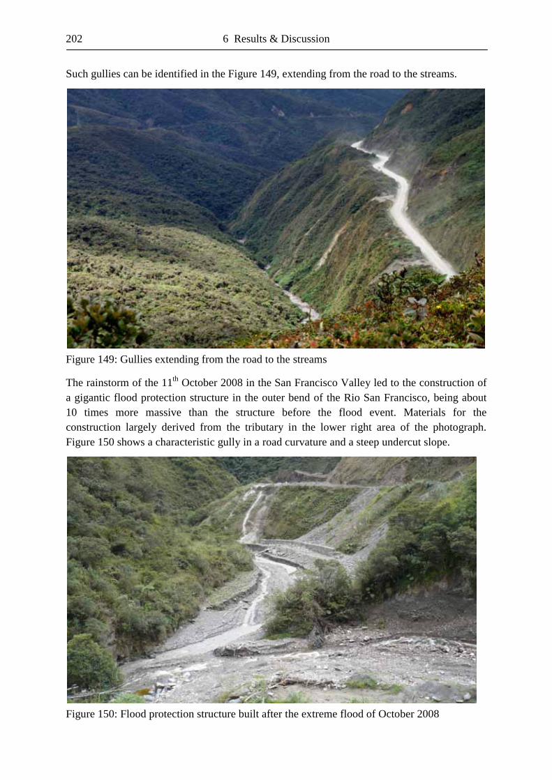
202 6 Results & Discussion

Such gullies can be identified in the Figure 149, extending from the road to the streams.

Figure 149: Gullies extending from the road to the streams

The rainstorm of the 11th October 2008 in the San Francisco Valley led to the construction of a gigantic flood protection structure in the outer bend of the Rio San Francisco, being about 10 times more massive than the structure before the flood event. Materials for the construction largely derived from the tributary in the lower right area of the photograph. Figure 150 shows a characteristic gully in a road curvature and a steep undercut slope.

Figure 150: Flood protection structure built after the extreme flood of October 2008

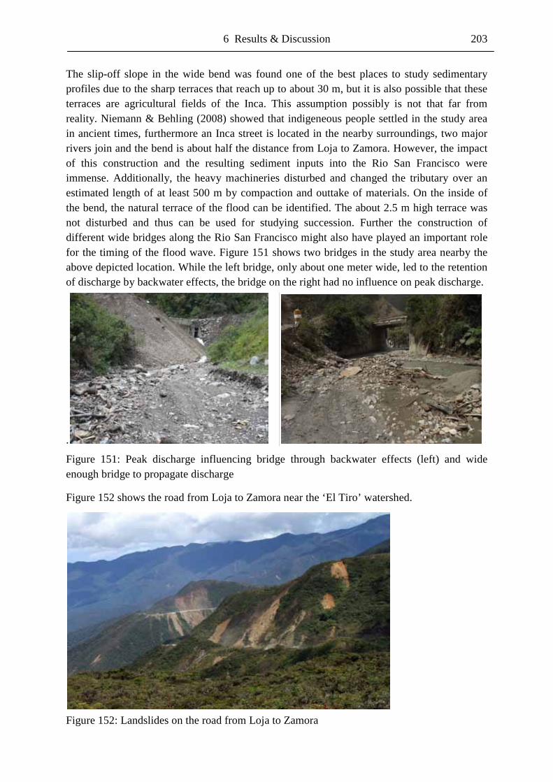
6 Results & Discussion 203

The slip-off slope in the wide bend was found one of the best places to study sedimentary profiles due to the sharp terraces that reach up to about 30 m, but it is also possible that these terraces are agricultural fields of the Inca. This assumption possibly is not that far from reality. Niemann & Behling (2008) showed that indigeneous people settled in the study area in ancient times, furthermore an Inca street is located in the nearby surroundings, two major rivers join and the bend is about half the distance from Loja to Zamora. However, the impact of this construction and the resulting sediment inputs into the Rio San Francisco were immense. Additionally, the heavy machineries disturbed and changed the tributary over an estimated length of at least 500 m by compaction and outtake of materials. On the inside of the bend, the natural terrace of the flood can be identified. The about 2.5 m high terrace was not disturbed and thus can be used for studying succession. Further the construction of different wide bridges along the Rio San Francisco might also have played an important role for the timing of the flood wave. Figure 151 shows two bridges in the study area nearby the above depicted location. While the left bridge, only about one meter wide, led to the retention of discharge by backwater effects, the bridge on the right had no influence on peak discharge.

.

Figure 151: Peak discharge influencing bridge through backwater effects (left) and wide enough bridge to propagate discharge

Figure 152 shows the road from Loja to Zamora near the ‘El Tiro’ watershed.

Figure 152: Landslides on the road from Loja to Zamora

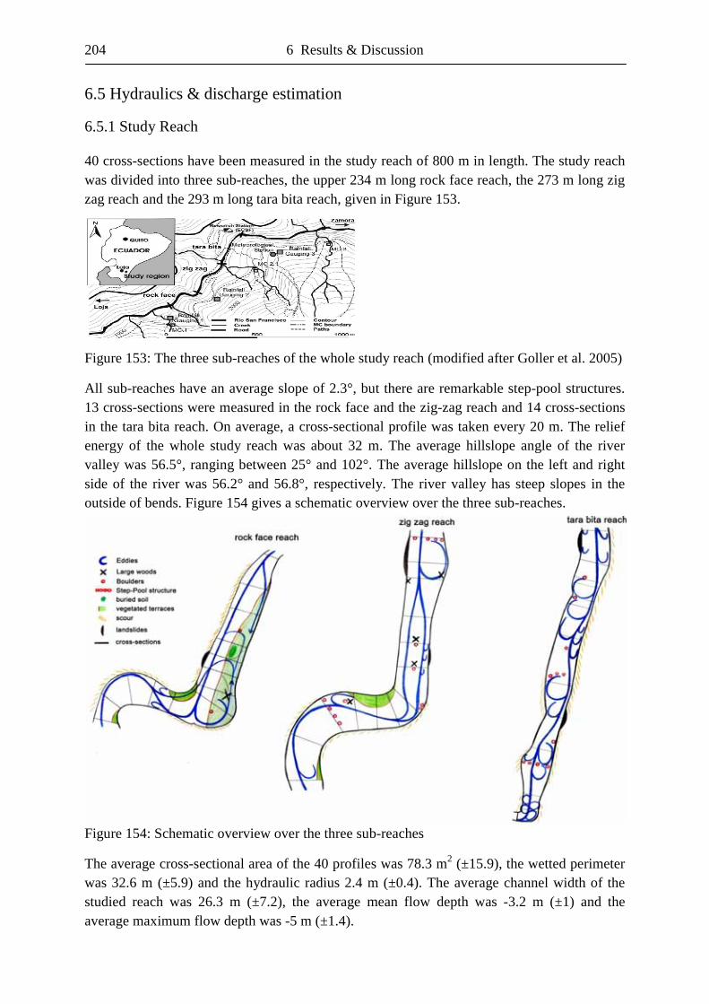
204 6 Results & Discussion

6.5 Hydraulics & discharge estimation

6.5.1 Study Reach

40 cross-sections have been measured in the study reach of 800 m in length. The study reach was divided into three sub-reaches, the upper 234 m long rock face reach, the 273 m long zig zag reach and the 293 m long tara bita reach, given in Figure 153.

Figure 153: The three sub-reaches of the whole study reach (modified after Goller et al. 2005)

All sub-reaches have an average slope of 2.3°, but there are remarkable step-pool structures. 13 cross-sections were measured in the rock face and the zig-zag reach and 14 cross-sections in the tara bita reach. On average, a cross-sectional profile was taken every 20 m. The relief energy of the whole study reach was about 32 m. The average hillslope angle of the river valley was 56.5°, ranging between 25° and 102°. The average hillslope on the left and right side of the river was 56.2° and 56.8°, respectively. The river valley has steep slopes in the outside of bends. Figure 154 gives a schematic overview over the three sub-reaches.

Figure 154: Schematic overview over the three sub-reaches

The average cross-sectional area of the 40 profiles was 78.3 m2 (±15.9), the wetted perimeter was 32.6 m (±5.9) and the hydraulic radius 2.4 m (±0.4). The average channel width of the studied reach was 26.3 m (±7.2), the average mean flow depth was -3.2 m (±1) and the average maximum flow depth was -5 m (±1.4).

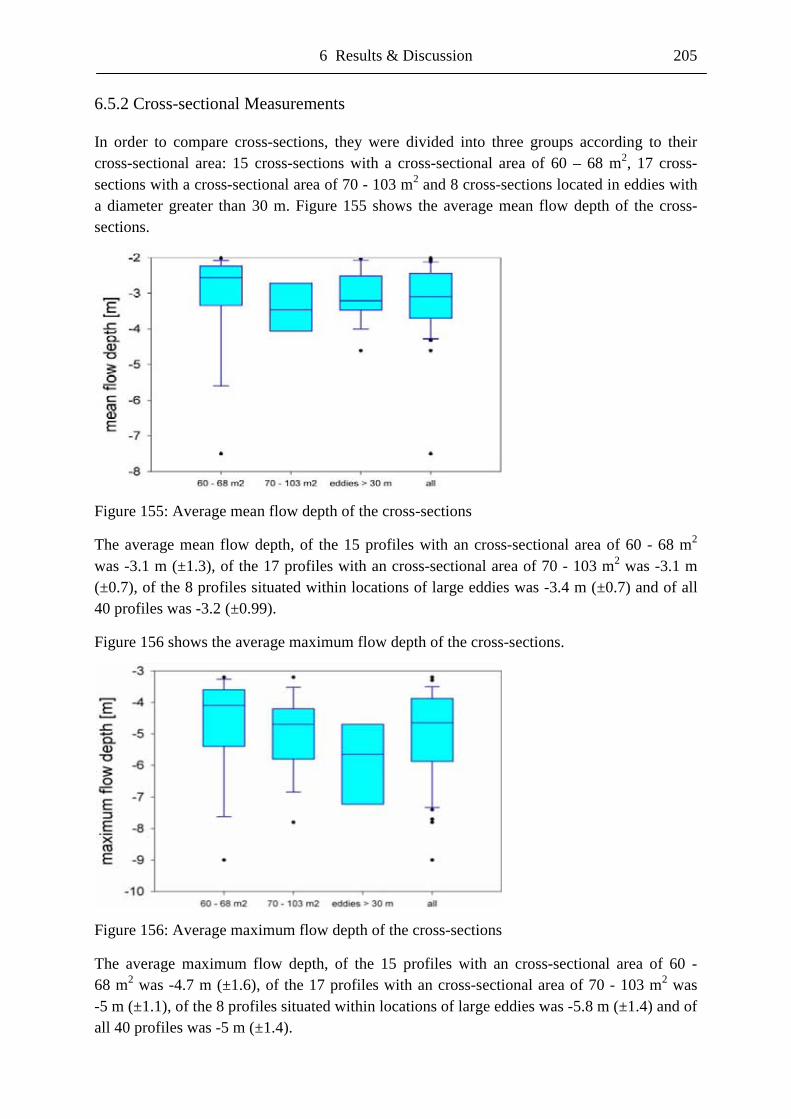
6 Results & Discussion 205

6.5.2 Cross-sectional Measurements

In order to compare cross-sections, they were divided into three groups according to their cross-sectional area: 15 cross-sections with a cross-sectional area of 60 – 68 m2, 17 cross-sections with a cross-sectional area of 70 - 103 m2 and 8 cross-sections located in eddies with a diameter greater than 30 m. Figure 155 shows the average mean flow depth of the cross-sections.

Figure 155: Average mean flow depth of the cross-sections

The average mean flow depth, of the 15 profiles with an cross-sectional area of 60 - 68 m2 was -3.1 m (±1.3), of the 17 profiles with an cross-sectional area of 70 - 103 m2 was -3.1 m (±0.7), of the 8 profiles situated within locations of large eddies was -3.4 m (±0.7) and of all 40 profiles was -3.2 (±0.99).

Figure 156 shows the average maximum flow depth of the cross-sections.

Figure 156: Average maximum flow depth of the cross-sections

The average maximum flow depth, of the 15 profiles with an cross-sectional area of 60 - 68 m2 was -4.7 m (±1.6), of the 17 profiles with an cross-sectional area of 70 - 103 m2 was -5 m (±1.1), of the 8 profiles situated within locations of large eddies was -5.8 m (±1.4) and of all 40 profiles was -5 m (±1.4).

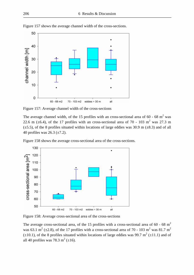
206 6 Results & Discussion

Figure 157 shows the average channel width of the cross-sections.

Figure 157: Average channel width of the cross-sections

The average channel width, of the 15 profiles with an cross-sectional area of 60 - 68 m2 was 22.6 m (±6.4), of the 17 profiles with an cross-sectional area of 70 - 103 m2 was 27.3 m (±5.5), of the 8 profiles situated within locations of large eddies was 30.9 m (±8.3) and of all 40 profiles was 26.3 (±7.2).

Figure 158 shows the average cross-sectional area of the cross-sections.

Figure 158: Average cross-sectional area of the cross-sections

The average cross-sectional area, of the 15 profiles with a cross-sectional area of 60 - 68 m2 was 63.1 m2 (±2.8), of the 17 profiles with a cross-sectional area of 70 - 103 m2 was 81.7 m2 (±10.1), of the 8 profiles situated within locations of large eddies was 99.7 m2 (±11.1) and of all 40 profiles was 78.3 m2 (±16).

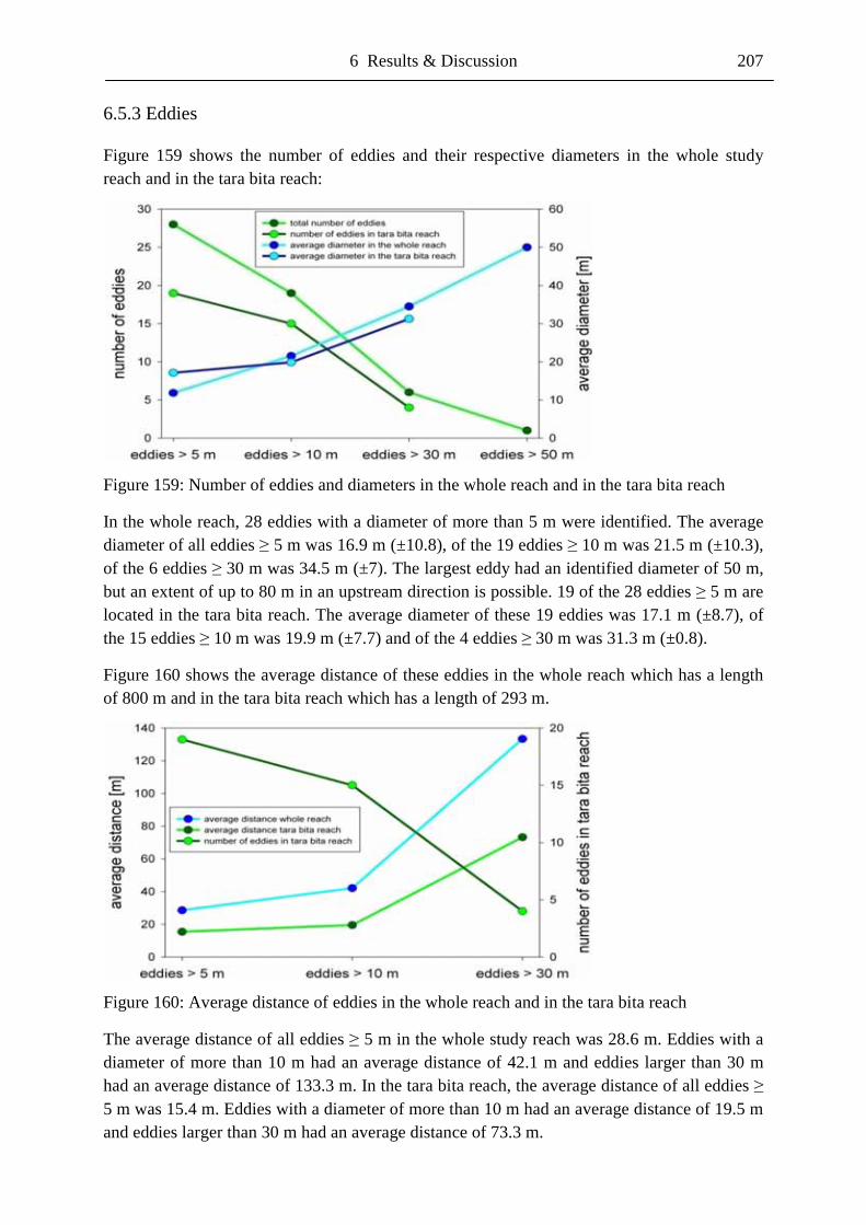
6 Results & Discussion 207

6.5.3 Eddies

Figure 159 shows the number of eddies and their respective diameters in the whole study reach and in the tara bita reach:

Figure 159: Number of eddies and diameters in the whole reach and in the tara bita reach

In the whole reach, 28 eddies with a diameter of more than 5 m were identified. The average diameter of all eddies � 5 m was 16.9 m (±10.8), of the 19 eddies � 10 m was 21.5 m (±10.3), of the 6 eddies � 30 m was 34.5 m (±7). The largest eddy had an identified diameter of 50 m, but an extent of up to 80 m in an upstream direction is possible. 19 of the 28 eddies � 5 m are located in the tara bita reach. The average diameter of these 19 eddies was 17.1 m (±8.7), of the 15 eddies � 10 m was 19.9 m (±7.7) and of the 4 eddies � 30 m was 31.3 m (±0.8).

Figure 160 shows the average distance of these eddies in the whole reach which has a length of 800 m and in the tara bita reach which has a length of 293 m.

Figure 160: Average distance of eddies in the whole reach and in the tara bita reach

The average distance of all eddies � 5 m in the whole study reach was 28.6 m. Eddies with a diameter of more than 10 m had an average distance of 42.1 m and eddies larger than 30 m had an average distance of 133.3 m. In the tara bita reach, the average distance of all eddies � 5 m was 15.4 m. Eddies with a diameter of more than 10 m had an average distance of 19.5 m and eddies larger than 30 m had an average distance of 73.3 m.

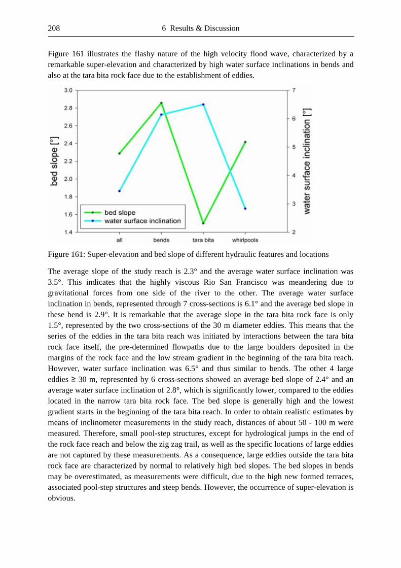
208 6 Results & Discussion

Figure 161 illustrates the flashy nature of the high velocity flood wave, characterized by a remarkable super-elevation and characterized by high water surface inclinations in bends and also at the tara bita rock face due to the establishment of eddies.

Figure 161: Super-elevation and bed slope of different hydraulic features and locations

The average slope of the study reach is 2.3° and the average water surface inclination was 3.5°. This indicates that the highly viscous Rio San Francisco was meandering due to gravitational forces from one side of the river to the other. The average water surface inclination in bends, represented through 7 cross-sections is 6.1° and the average bed slope in these bend is 2.9°. It is remarkable that the average slope in the tara bita rock face is only 1.5°, represented by the two cross-sections of the 30 m diameter eddies. This means that the series of the eddies in the tara bita reach was initiated by interactions between the tara bita rock face itself, the pre-determined flowpaths due to the large boulders deposited in the margins of the rock face and the low stream gradient in the beginning of the tara bita reach. However, water surface inclination was 6.5° and thus similar to bends. The other 4 large eddies � 30 m, represented by 6 cross-sections showed an average bed slope of 2.4° and an average water surface inclination of 2.8°, which is significantly lower, compared to the eddies located in the narrow tara bita rock face. The bed slope is generally high and the lowest gradient starts in the beginning of the tara bita reach. In order to obtain realistic estimates by means of inclinometer measurements in the study reach, distances of about 50 - 100 m were measured. Therefore, small pool-step structures, except for hydrological jumps in the end of the rock face reach and below the zig zag trail, as well as the specific locations of large eddies are not captured by these measurements. As a consequence, large eddies outside the tara bita rock face are characterized by normal to relatively high bed slopes. The bed slopes in bends may be overestimated, as measurements were difficult, due to the high new formed terraces, associated pool-step structures and steep bends. However, the occurrence of super-elevation is obvious.

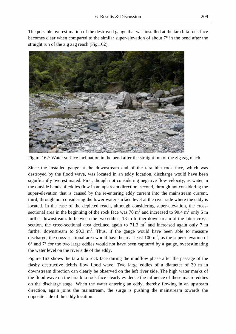
6 Results & Discussion 209

The possible overestimation of the destroyed gauge that was installed at the tara bita rock face becomes clear when compared to the similar super-elevation of about 7° in the bend after the straight run of the zig zag reach (Fig.162).

Figure 162: Water surface inclination in the bend after the straight run of the zig zag reach

Since the installed gauge at the downstream end of the tara bita rock face, which was destroyed by the flood wave, was located in an eddy location, discharge would have been significantly overestimated. First, though not considering negative flow velocity, as water in the outside bends of eddies flow in an upstream direction, second, through not considering the super-elevation that is caused by the re-entering eddy current into the mainstream current, third, through not considering the lower water surface level at the river side where the eddy is located. In the case of the depicted reach, although considering super-elevation, the cross-sectional area in the beginning of the rock face was 70 m2 and increased to 90.4 m2 only 5 m further downstream. In between the two eddies, 13 m further downstream of the latter cross-section, the cross-sectional area declined again to 71.3 m2 and increased again only 7 m further downstream to 90.3 m2. Thus, if the gauge would have been able to measure discharge, the cross-sectional area would have been at least 100 m2, as the super-elevation of 6° and 7° for the two large eddies would not have been captured by a gauge, overestimating the water level on the river side of the eddy.

Figure 163 shows the tara bita rock face during the mudflow phase after the passage of the flashy destructive debris flow flood wave. Two large eddies of a diameter of 30 m in downstream direction can clearly be observed on the left river side. The high water marks of the flood wave on the tara bita rock face clearly evidence the influence of these macro eddies on the discharge stage. When the water entering an eddy, thereby flowing in an upstream direction, again joins the mainstream, the surge is pushing the mainstream towards the opposite side of the eddy location.

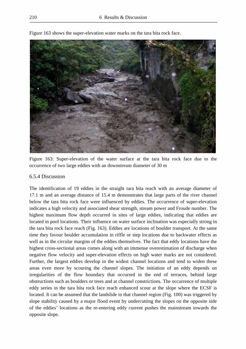
210 6 Results & Discussion

Figure 163 shows the super-elevation water marks on the tara bita rock face.

Figure 163: Super-elevation of the water surface at the tara bita rock face due to the occurrence of two large eddies with an downstream diameter of 30 m

6.5.4 Discussion

The identification of 19 eddies in the straight tara bita reach with an average diameter of 17.1 m and an average distance of 15.4 m demonstrates that large parts of the river channel below the tara bita rock face were influenced by eddies. The occurrence of super-elevation indicates a high velocity and associated shear strength, stream power and Froude number. The highest maximum flow depth occurred in sites of large eddies, indicating that eddies are located in pool locations. Their influence on water surface inclination was especially strong in the tara bita rock face reach (Fig. 163). Eddies are locations of boulder transport. At the same time they favour boulder accumulation in riffle or step locations due to backwater effects as well as in the circular margins of the eddies themselves. The fact that eddy locations have the highest cross-sectional areas comes along with an immense overestimation of discharge when negative flow velocity and super-elevation effects on high water marks are not considered. Further, the largest eddies develop in the widest channel locations and tend to widen these areas even more by scouring the channel slopes. The initiation of an eddy depends on irregularities of the flow boundary that occurred in the end of terraces, behind large obstructions such as boulders or trees and at channel constrictions. The occurrence of multiple eddy series in the tara bita rock face reach enhanced scour at the slope where the ECSF is located. It can be assumed that the landslide in that channel region (Fig. 100) was triggered by slope stability caused by a major flood event by undercutting the slopes on the opposite side of the eddies’ locations as the re-entering eddy current pushes the mainstream towards the opposite slope.

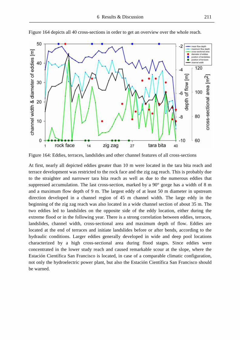
6 Results & Discussion 211

Figure 164 depicts all 40 cross-sections in order to get an overview over the whole reach.

Figure 164: Eddies, terraces, landslides and other channel features of all cross-sections

At first, nearly all depicted eddies greater than 10 m were located in the tara bita reach and terrace development was restricted to the rock face and the zig zag reach. This is probably due to the straighter and narrower tara bita reach as well as due to the numerous eddies that suppressed accumulation. The last cross-section, marked by a 90° gorge has a width of 8 m and a maximum flow depth of 9 m. The largest eddy of at least 50 m diameter in upstream direction developed in a channel region of 45 m channel width. The large eddy in the beginning of the zig zag reach was also located in a wide channel section of about 35 m. The two eddies led to landslides on the opposite side of the eddy location, either during the extreme flood or in the following year. There is a strong correlation between eddies, terraces, landslides, channel width, cross-sectional area and maximum depth of flow. Eddies are located at the end of terraces and initiate landslides before or after bends, according to the hydraulic conditions. Larger eddies generally developed in wide and deep pool locations characterized by a high cross-sectional area during flood stages. Since eddies were concentrated in the lower study reach and caused remarkable scour at the slope, where the Estación Científica San Francisco is located, in case of a comparable climatic configuration, not only the hydroelectric power plant, but also the Estación Científica San Francisco should be warned.

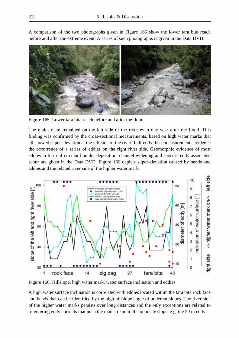
212 6 Results & Discussion

A comparison of the two photographs given in Figure 165 show the lower tara bita reach before and after the extreme event. A series of such photographs is given in the Data DVD.

Figure 165: Lower tara bita reach before and after the flood

The mainstream remained on the left side of the river even one year after the flood. This finding was confirmed by the cross-sectional measurements, based on high water marks that all showed super-elevation at the left side of the river. Indirectly these measurements evidence the occurrence of a series of eddies on the right river side. Geomorphic evidence of most eddies in form of circular boulder deposition, channel widening and specific eddy associated scour are given in the Data DVD. Figure 166 depicts super-elevation caused by bends and eddies and the related river side of the higher water mark.

Figure 166: Hillslope, high water mark, water surface inclination and eddies

A high water surface inclination is correlated with eddies located within the tara bita rock face and bends that can be identified by the high hillslope angle of undercut slopes. The river side of the higher water marks persists over long distances and the only exceptions are related to re-entering eddy currents that push the mainstream to the opposite slope, e.g. the 50 m eddy.

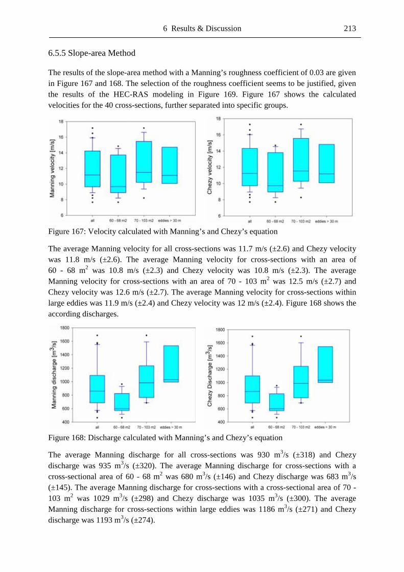
6 Results & Discussion 213

6.5.5 Slope-area Method

The results of the slope-area method with a Manning’s roughness coefficient of 0.03 are given in Figure 167 and 168. The selection of the roughness coefficient seems to be justified, given the results of the HEC-RAS modeling in Figure 169. Figure 167 shows the calculated velocities for the 40 cross-sections, further separated into specific groups.

Figure 167: Velocity calculated with Manning’s and Chezy’s equation

The average Manning velocity for all cross-sections was 11.7 m/s (±2.6) and Chezy velocity was 11.8 m/s (±2.6). The average Manning velocity for cross-sections with an area of 60 - 68 m2 was 10.8 m/s (±2.3) and Chezy velocity was 10.8 m/s (±2.3). The average Manning velocity for cross-sections with an area of 70 - 103 m2 was 12.5 m/s (±2.7) and Chezy velocity was 12.6 m/s (±2.7). The average Manning velocity for cross-sections within large eddies was 11.9 m/s (±2.4) and Chezy velocity was 12 m/s (±2.4). Figure 168 shows the according discharges.

Figure 168: Discharge calculated with Manning’s and Chezy’s equation

The average Manning discharge for all cross-sections was 930 m3/s (±318) and Chezy discharge was 935 m3/s (±320). The average Manning discharge for cross-sections with a cross-sectional area of 60 - 68 m2 was 680 m3/s (±146) and Chezy discharge was 683 m3/s (±145). The average Manning discharge for cross-sections with a cross-sectional area of 70 - 103 m2 was 1029 m3/s (±298) and Chezy discharge was 1035 m3/s (±300). The average Manning discharge for cross-sections within large eddies was 1186 m3/s (±271) and Chezy discharge was 1193 m3/s (±274).

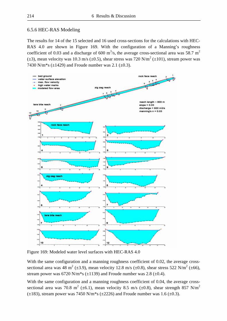
214 6 Results & Discussion

6.5.6 HEC-RAS Modeling

The results for 14 of the 15 selected and 16 used cross-sections for the calculations with HEC-RAS 4.0 are shown in Figure 169. With the configuration of a Manning’s roughness coefficient of 0.03 and a discharge of 600 m3/s, the average cross-sectional area was 58.7 m2 (±3), mean velocity was 10.3 m/s (±0.5), shear stress was 720 N/m2 (±101), stream power was 7430 N/m*s (±1429) and Froude number was 2.1 (±0.3).

Figure 169: Modeled water level surfaces with HEC-RAS 4.0

With the same configuration and a manning roughness coefficient of 0.02, the average cross-sectional area was 48 m2 (±3.9), mean velocity 12.8 m/s (±0.8), shear stress 522 N/m2 (±66), stream power was 6720 N/m*s (±1139) and Froude number was 2.8 (±0.4).

With the same configuration and a manning roughness coefficient of 0.04, the average cross-sectional area was 70.8 m2 (±6.1), mean velocity 8.5 m/s (±0.8), shear strength 857 N/m2 (±183), stream power was 7450 N/m*s (±2226) and Froude number was 1.6 (±0.3).

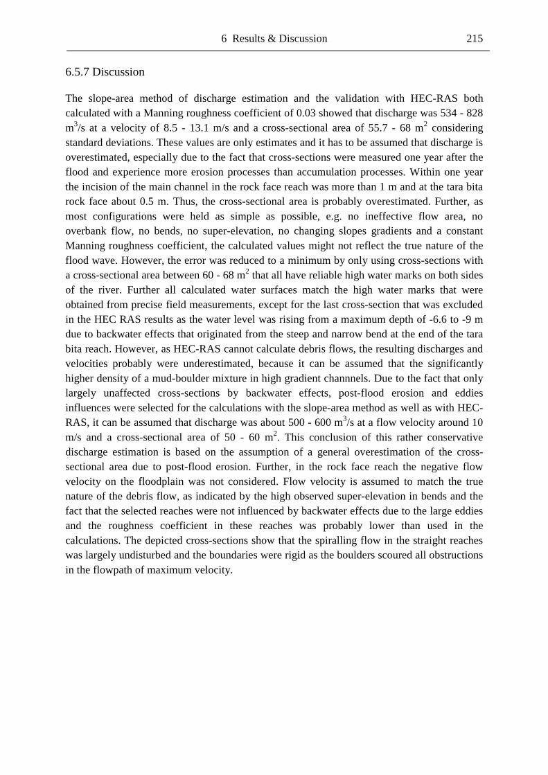
6 Results & Discussion 215

6.5.7 Discussion

The slope-area method of discharge estimation and the validation with HEC-RAS both calculated with a Manning roughness coefficient of 0.03 showed that discharge was 534 - 828 m3/s at a velocity of 8.5 - 13.1 m/s and a cross-sectional area of 55.7 - 68 m2 considering standard deviations. These values are only estimates and it has to be assumed that discharge is overestimated, especially due to the fact that cross-sections were measured one year after the flood and experience more erosion processes than accumulation processes. Within one year the incision of the main channel in the rock face reach was more than 1 m and at the tara bita rock face about 0.5 m. Thus, the cross-sectional area is probably overestimated. Further, as most configurations were held as simple as possible, e.g. no ineffective flow area, no overbank flow, no bends, no super-elevation, no changing slopes gradients and a constant Manning roughness coefficient, the calculated values might not reflect the true nature of the flood wave. However, the error was reduced to a minimum by only using cross-sections with a cross-sectional area between 60 - 68 m2 that all have reliable high water marks on both sides of the river. Further all calculated water surfaces match the high water marks that were obtained from precise field measurements, except for the last cross-section that was excluded in the HEC RAS results as the water level was rising from a maximum depth of -6.6 to -9 m due to backwater effects that originated from the steep and narrow bend at the end of the tara bita reach. However, as HEC-RAS cannot calculate debris flows, the resulting discharges and velocities probably were underestimated, because it can be assumed that the significantly higher density of a mud-boulder mixture in high gradient channnels. Due to the fact that only largely unaffected cross-sections by backwater effects, post-flood erosion and eddies influences were selected for the calculations with the slope-area method as well as with HEC-RAS, it can be assumed that discharge was about 500 - 600 m3/s at a flow velocity around 10 m/s and a cross-sectional area of 50 - 60 m2. This conclusion of this rather conservative discharge estimation is based on the assumption of a general overestimation of the cross-sectional area due to post-flood erosion. Further, in the rock face reach the negative flow velocity on the floodplain was not considered. Flow velocity is assumed to match the true nature of the debris flow, as indicated by the high observed super-elevation in bends and the fact that the selected reaches were not influenced by backwater effects due to the large eddies and the roughness coefficient in these reaches was probably lower than used in the calculations. The depicted cross-sections show that the spiralling flow in the straight reaches was largely undisturbed and the boundaries were rigid as the boulders scoured all obstructions in the flowpath of maximum velocity.

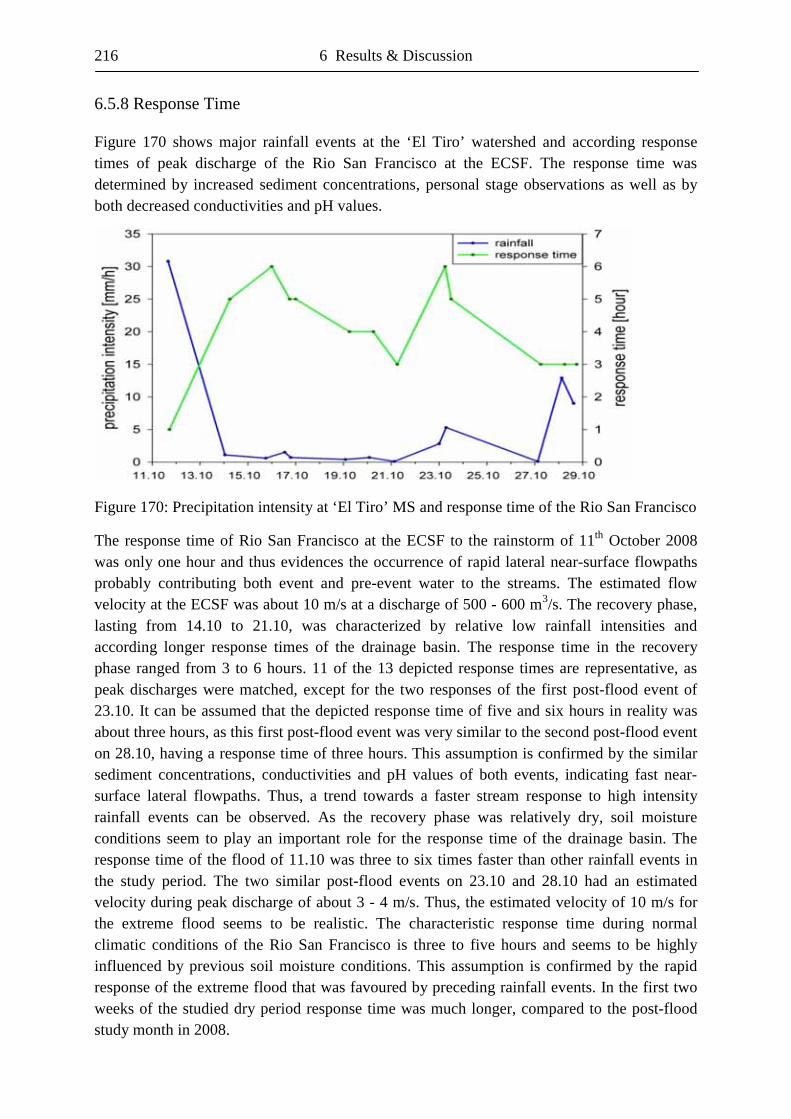
216 6 Results & Discussion

6.5.8 Response Time

Figure 170 shows major rainfall events at the ‘El Tiro’ watershed and according response times of peak discharge of the Rio San Francisco at the ECSF. The response time was determined by increased sediment concentrations, personal stage observations as well as by both decreased conductivities and pH values.

Figure 170: Precipitation intensity at ‘El Tiro’ MS and response time of the Rio San Francisco

The response time of Rio San Francisco at the ECSF to the rainstorm of 11th October 2008 was only one hour and thus evidences the occurrence of rapid lateral near-surface flowpaths probably contributing both event and pre-event water to the streams. The estimated flow velocity at the ECSF was about 10 m/s at a discharge of 500 - 600 m3/s. The recovery phase, lasting from 14.10 to 21.10, was characterized by relative low rainfall intensities and according longer response times of the drainage basin. The response time in the recovery phase ranged from 3 to 6 hours. 11 of the 13 depicted response times are representative, as peak discharges were matched, except for the two responses of the first post-flood event of 23.10. It can be assumed that the depicted response time of five and six hours in reality was about three hours, as this first post-flood event was very similar to the second post-flood event on 28.10, having a response time of three hours. This assumption is confirmed by the similar sediment concentrations, conductivities and pH values of both events, indicating fast near-surface lateral flowpaths. Thus, a trend towards a faster stream response to high intensity rainfall events can be observed. As the recovery phase was relatively dry, soil moisture conditions seem to play an important role for the response time of the drainage basin. The response time of the flood of 11.10 was three to six times faster than other rainfall events in the study period. The two similar post-flood events on 23.10 and 28.10 had an estimated velocity during peak discharge of about 3 - 4 m/s. Thus, the estimated velocity of 10 m/s for the extreme flood seems to be realistic. The characteristic response time during normal climatic conditions of the Rio San Francisco is three to five hours and seems to be highly influenced by previous soil moisture conditions. This assumption is confirmed by the rapid response of the extreme flood that was favoured by preceding rainfall events. In the first two weeks of the studied dry period response time was much longer, compared to the post-flood study month in 2008.

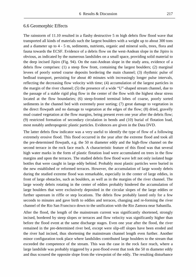
6 Results & Discussion 217

6.6 Geomorphic Effects

The rainstorm of 11.10 resulted in a flashy destructive 5 m high debris flow flood wave that transported all kinds of materials such the largest boulders with a weight up to about 300 tons and a diameter up to 4 - 5 m, sediments, nutrients, organic and mineral soils, trees, flora and fauna towards the ECSF. Evidence of a debris flow on the west-Andean slope in the Jipiro is obvious, as indicated by the numerous landslides on a small space, providing solid material to the deep incised Jipiro (Fig. 94). On the east-Andean slope in the study area, evidence of a debris flow comprises: (1) a steep flow front, containing the largest boulders; (2) marginal levees of poorly sorted coarse deposits bordering the main channel; (3) rhythmic pulse of bedload transport, persisting for about 40 minutes with increasingly longer pulse intervals, reflecting the decreasing flow velocity with time; (4) accumulation of the largest particles in the margin of the river channel; (5) the presence of a wide “U”-shaped stream channel, due to the passage of a stable rigid plug flow in the center of the flow with the highest shear stress located at the flow boundaries; (6) steep-fronted terminal lobes of coarse, poorly sorted sediments in the channel bed with extremely poor sorting; (7) great damage to vegetation in the direct flowpath and no damage to vegetation at the edges of the flow; (8) dried, gravelly mud coated vegetation at the flow margins, being present even one year after the debris flow; (9) restricted formation of secondary circulation in bends and (10) burial of flotation load, most notably anthropogenic plastic particles. Evidences are given in the Data DVD.

The latter debris flow indicator was a very useful to identify the type of flow of a following extremely erosive flood. This flood occurred in the year after the extreme flood and took all the pre-determined flowpath, e.g. the 50 m diameter eddy and the high-flow channel on the second terrace in the rock face reach. A characteristic feature of this flood was that several high water marks in the form of plastic flotation load were accumulated on trees in the flow margins and upon the terraces. The studied debris flow flood wave left not only isolated huge bottles that were caught in large eddy behind. Probably most plastic particles were buried in the new established or reformed terraces. However, the accumulation of large woody debris during the studied extreme flood was remarkable, especially in the center of large eddies, in front of large obstacles, such as boulders, as well as in the margins of the river channel. The large woody debris rotating in the center of eddies probably hindered the accumulation of large boulders that were exclusively deposited in the circular slopes of the large eddies or further upstream in riffle or step locations. The debris flow probably lasted only for a few seconds to minutes and gave birth to eddies and terraces, changing and re-forming the river channel of the Rio San Francisco down to the unification with the Rio Zamora near Sabanilla.

After the flood, the length of the mainstream current was significantly shortened, strongly incised, bordered by steep slopes or terraces and flow velocity was significantly higher than before the flood event at the same discharge stages. Even one year after the flood, the river remained in the pre-determined river bed, except were slip-off slopes have been eroded and the river had incised, thus shortening the mainstream channel length even further. Another minor configuration took place where landslides contributed large boulders to the stream that exceeded the competence of the stream. This was the case in the rock face reach, where a large landslide was probably triggered by a post-flood event that took the 50 m diameter eddy and thus scoured the opposite slope from the viewpoint of the eddy. The resulting disturbance

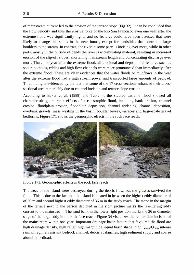
218 6 Results & Discussion

of mainstream current led to the erosion of the terrace slope (Fig.32). It can be concluded that the flow velocity and thus the erosive force of the Rio San Francisco even one year after the extreme flood was significantly higher and no features could have been detected that were likely to change this status in the near future, except for landslides that contribute large boulders to the stream. In contrast, the river in some parts is incising ever more, while in other parts, mostly in the outside of bends the river is accumulating material, resulting in increased erosion of the slip-off slopes, shortening mainstream length and concentrating discharge ever more. Thus, one year after the extreme flood, all erosional and depositional features such as scour, potholes, eddies and high flow channels were more pronounced than immediately after the extreme flood. These are clear evidences that the water floods or mudflows in the year after the extreme flood had a high stream power and transported large amounts of bedload. This finding is evidenced by the fact that some of the 17 cross-sections enhanced their cross-sectional area remarkably due to channel incision and terrace slope erosion.

According to Baker et al. (1988) and Table 4, the studied extreme flood showed all characteristic geomorphic effects of a catastrophic flood, including bank erosion, channel erosion, floodplain erosion, floodplain deposition, channel widening, channel deposition, overbank gravels, mass wasting in the basin, boulder levees, terraces and large-scale gravel bedforms. Figure 171 shows the geomorphic effects in the rock face reach.

Figure 171: Geomorphic effects in the rock face reach

The trees of the island were destroyed during the debris flow, but the grasses survived the flood. This is due to the fact that the island is located in between the highest eddy diameter of of 50 m and second highest eddy diameter of 36 m in the study reach. The stone in the margin of the terrace next to the person depicted in the right picture marks the re-entering eddy current to the mainstream. The sand bank in the lower right position marks the 36 m diameter stage of the large eddy in the rock face reach. Figure 34 visualizes the remarkable incision of the mainstream within one year. Important drainage basin factors that favoured the flood are high drainage density, high relief, high magnitude, equal basin shape, high Qmax/Qmin, intense rainfall regime, resistant bedrock channel, debris avalanches, high sediment supply and coarse abundant bedload.

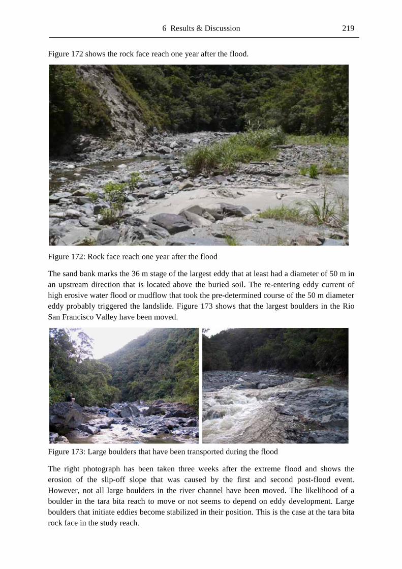
6 Results & Discussion 219

Figure 172 shows the rock face reach one year after the flood.

Figure 172: Rock face reach one year after the flood

The sand bank marks the 36 m stage of the largest eddy that at least had a diameter of 50 m in an upstream direction that is located above the buried soil. The re-entering eddy current of high erosive water flood or mudflow that took the pre-determined course of the 50 m diameter eddy probably triggered the landslide. Figure 173 shows that the largest boulders in the Rio San Francisco Valley have been moved.

Figure 173: Large boulders that have been transported during the flood

The right photograph has been taken three weeks after the extreme flood and shows the erosion of the slip-off slope that was caused by the first and second post-flood event. However, not all large boulders in the river channel have been moved. The likelihood of a boulder in the tara bita reach to move or not seems to depend on eddy development. Large boulders that initiate eddies become stabilized in their position. This is the case at the tara bita rock face in the study reach.

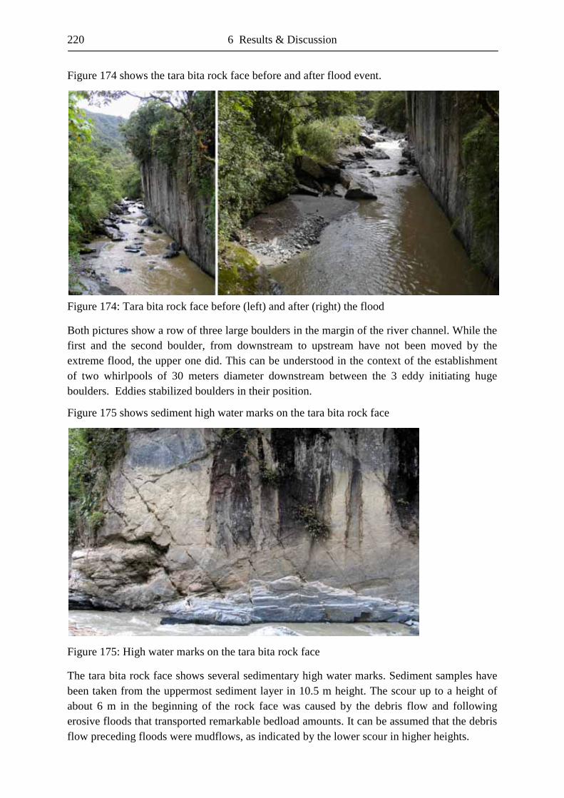
220 6 Results & Discussion

Figure 174 shows the tara bita rock face before and after flood event.

Figure 174: Tara bita rock face before (left) and after (right) the flood

Both pictures show a row of three large boulders in the margin of the river channel. While the first and the second boulder, from downstream to upstream have not been moved by the extreme flood, the upper one did. This can be understood in the context of the establishment of two whirlpools of 30 meters diameter downstream between the 3 eddy initiating huge boulders. Eddies stabilized boulders in their position. Figure 175 shows sediment high water marks on the tara bita rock face

Figure 175: High water marks on the tara bita rock face

The tara bita rock face shows several sedimentary high water marks. Sediment samples have been taken from the uppermost sediment layer in 10.5 m height. The scour up to a height of about 6 m in the beginning of the rock face was caused by the debris flow and following erosive floods that transported remarkable bedload amounts. It can be assumed that the debris flow preceding floods were mudflows, as indicated by the lower scour in higher heights.

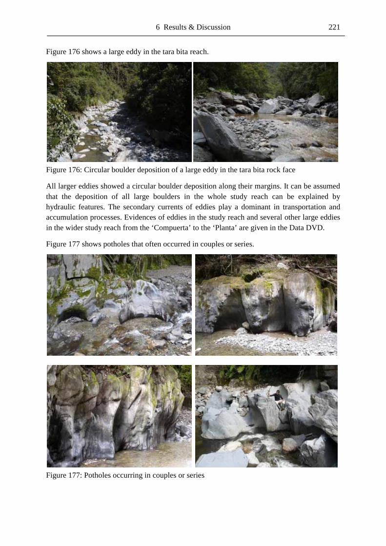
6 Results & Discussion 221

Figure 176 shows a large eddy in the tara bita reach.

Figure 176: Circular boulder deposition of a large eddy in the tara bita rock face

All larger eddies showed a circular boulder deposition along their margins. It can be assumed that the deposition of all large boulders in the whole study reach can be explained by hydraulic features. The secondary currents of eddies play a dominant in transportation and accumulation processes. Evidences of eddies in the study reach and several other large eddies in the wider study reach from the ‘Compuerta’ to the ‘Planta’ are given in the Data DVD.

Figure 177 shows potholes that often occurred in couples or series.

Figure 177: Potholes occurring in couples or series

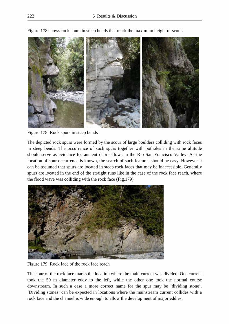
222 6 Results & Discussion

Figure 178 shows rock spurs in steep bends that mark the maximum height of scour.

Figure 178: Rock spurs in steep bends

The depicted rock spurs were formed by the scour of large boulders colliding with rock faces in steep bends. The occurrence of such spurs together with potholes in the same altitude should serve as evidence for ancient debris flows in the Rio San Francisco Valley. As the location of spur occurrence is known, the search of such features should be easy. However it can be assumed that spurs are located in steep rock faces that may be inaccessible. Generally spurs are located in the end of the straight runs like in the case of the rock face reach, where the flood wave was colliding with the rock face (Fig.179).

Figure 179: Rock face of the rock face reach

The spur of the rock face marks the location where the main current was divided. One current took the 50 m diameter eddy to the left, while the other one took the normal course downstream. In such a case a more correct name for the spur may be ‘dividing stone’. ‘Dividing stones’ can be expected in locations where the mainstream current collides with a rock face and the channel is wide enough to allow the development of major eddies.

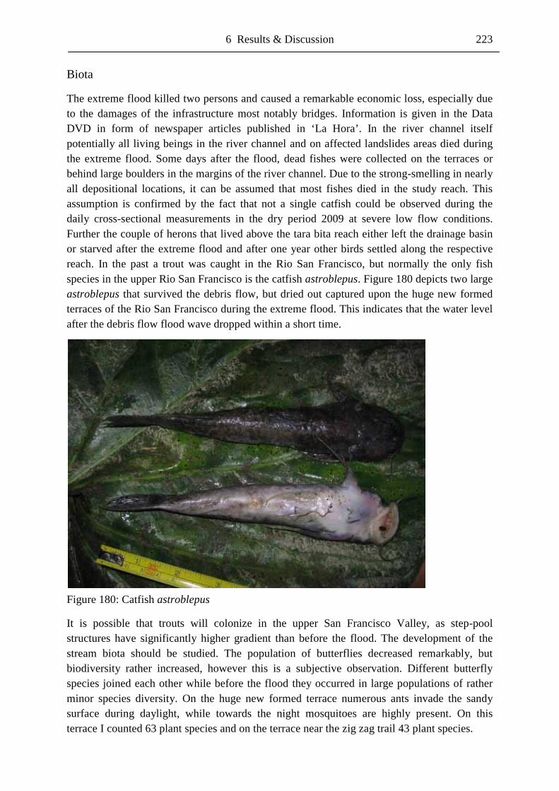
6 Results & Discussion 223

Biota

The extreme flood killed two persons and caused a remarkable economic loss, especially due to the damages of the infrastructure most notably bridges. Information is given in the Data DVD in form of newspaper articles published in ‘La Hora’. In the river channel itself potentially all living beings in the river channel and on affected landslides areas died during the extreme flood. Some days after the flood, dead fishes were collected on the terraces or behind large boulders in the margins of the river channel. Due to the strong-smelling in nearly all depositional locations, it can be assumed that most fishes died in the study reach. This assumption is confirmed by the fact that not a single catfish could be observed during the daily cross-sectional measurements in the dry period 2009 at severe low flow conditions. Further the couple of herons that lived above the tara bita reach either left the drainage basin or starved after the extreme flood and after one year other birds settled along the respective reach. In the past a trout was caught in the Rio San Francisco, but normally the only fish species in the upper Rio San Francisco is the catfish astroblepus. Figure 180 depicts two large astroblepus that survived the debris flow, but dried out captured upon the huge new formed terraces of the Rio San Francisco during the extreme flood. This indicates that the water level after the debris flow flood wave dropped within a short time.

Figure 180: Catfish astroblepus

It is possible that trouts will colonize in the upper San Francisco Valley, as step-pool structures have significantly higher gradient than before the flood. The development of the stream biota should be studied. The population of butterflies decreased remarkably, but biodiversity rather increased, however this is a subjective observation. Different butterfly species joined each other while before the flood they occurred in large populations of rather minor species diversity. On the huge new formed terrace numerous ants invade the sandy surface during daylight, while towards the night mosquitoes are highly present. On this terrace I counted 63 plant species and on the terrace near the zig zag trail 43 plant species.

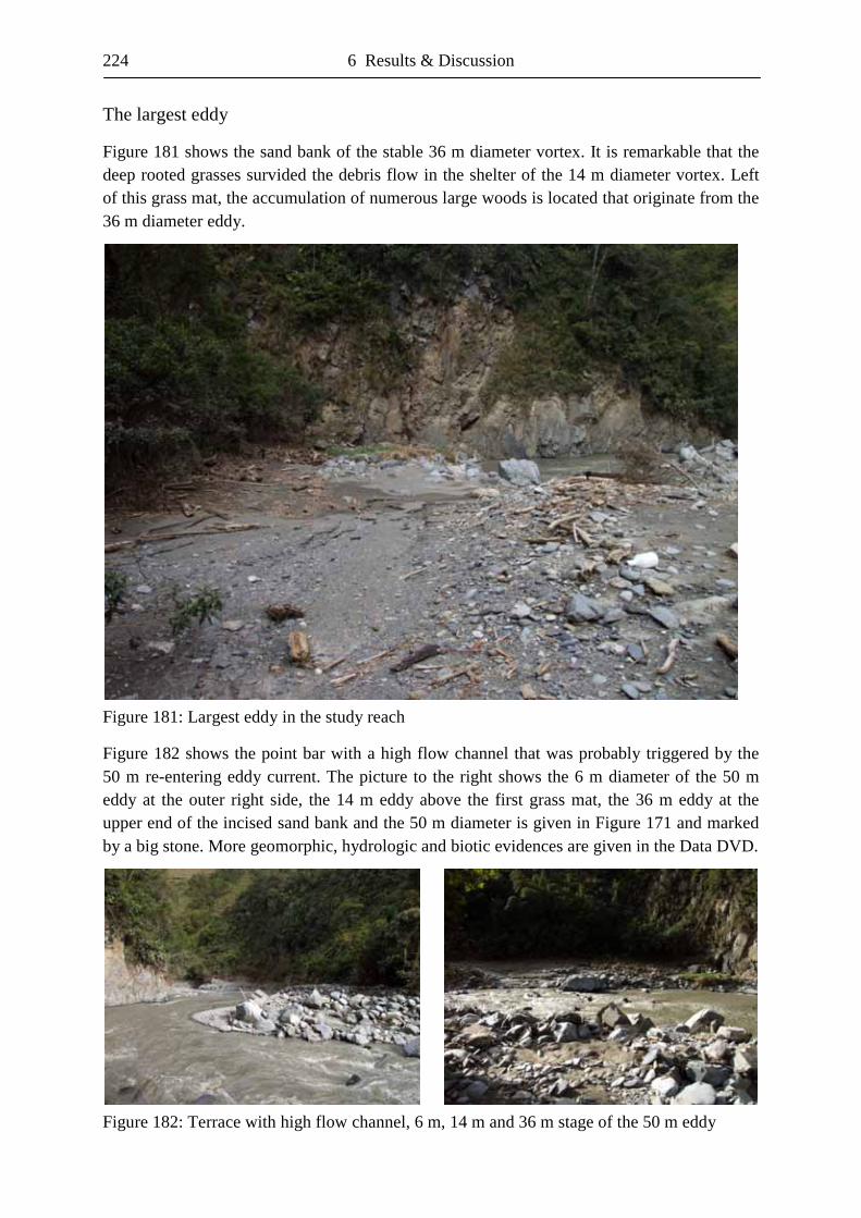
224 6 Results & Discussion

The largest eddy

Figure 181 shows the sand bank of the stable 36 m diameter vortex. It is remarkable that the deep rooted grasses survided the debris flow in the shelter of the 14 m diameter vortex. Left of this grass mat, the accumulation of numerous large woods is located that originate from the 36 m diameter eddy.

Figure 181: Largest eddy in the study reach

Figure 182 shows the point bar with a high flow channel that was probably triggered by the 50 m re-entering eddy current. The picture to the right shows the 6 m diameter of the 50 m eddy at the outer right side, the 14 m eddy above the first grass mat, the 36 m eddy at the upper end of the incised sand bank and the 50 m diameter is given in Figure 171 and marked by a big stone. More geomorphic, hydrologic and biotic evidences are given in the Data DVD.

Figure 182: Terrace with high flow channel, 6 m, 14 m and 36 m stage of the 50 m eddy

7 Conclusion 225

7 Conclusion

The objective of this study was to determine features of the extreme flood. Drainage basin factors that favoured the flood were: the circular drainage basin shape, the steep slopes, the high stream gradients, many first-order streams, intense gullying, high drainage density and a confined U-shaped bedrock main river channel with V-shaped tributaries. Furthermore, the densely rooted organic layers in forested soils have a high porosity and are characterized by a decreasing hydraulic conductivity with soil depth, favouring rapid near-surface flowpaths, especially due to the high soil saturation conditions as a consequence of the per-humid climate throughout the year. The increasing thickness of the organic layers with increasing altitude favours infiltration-excess overland flow and organic matrix flow. The increasingly coarser texture, characterised by higher sand contents and lower clay contents with altitude, probably increase the hydraulic conductivity with increasing altitude. The opening up of the vegetation and the decreasing canopy heights of the vegetation with increasing altitude favour the concentration of runoff in the hillslope hollows at the foot of the convergent slopes. This is due to the higher interception losses in lower altitudes and in valley locations, compared to higher altitudes and ridge positions.

Anthropogenic influences, most notably the road from Loja to Zamora and the ‘Camino Canal’ of the hydroelectric power plant ‘Planta’, concentrate runoff as well. In the dry period of 2009 the water outtake of the hydroelectric power plant led to severe low flow conditions in the study reach of the Rio San Francisco nearby the ECSF. Near-surface lateral flowpaths and rapid subsurface stormflow are favoured by macropores and pipes in the porous organic layers. A concentration of such flowpaths can be expected between the mineral soil and the organic soil due to the decreasing hydraulic conductivity with depth. Infiltration-excess overland flow is mainly generated in higher altitudes, while in lower altitudes saturation-excess overland flow should be dominant, as the overland flow infiltrates into the ever more forested slopes located downhill. Thus, pressure waves are very likely to produce return flow. In regions of lower relief water logging occurs, e.g. in the flat basins below the ‘El Tiro’ watershed. The high water table within the soil favours saturation-excess overland flow.

Climatic factors that favoured the flood were: rainfall events before the rainstorm leading to high soil saturation conditions, an extreme gradient of air temperature accompanied by high insolation and evapotranspiration after the invasion of ‘Veranillos de Niño’ immediately before the rainstorm, the establishment of upward moving convective clouds near the watersheds and the convergence of air masses from the Amazonian lowland rainforest and a thunderstorm originating from the Pacific Ocean. Furthermore, possibly additional air masses from surrounding areas, e.g. from the Reserve Podocarpus south of the drainage basin were advected. The sudden change in Sea Surface Temperature in the Pacific Ocean might also have contributed to the magnitude of the rainstorm. The convergent air masses led to low wind velocities, rapid upward motions and resulted in a short and high intensity rainfall event that was largely confined to the ‘El Tiro’ watershed. It can be assumed that the convergent air masses throughout the study period were involved in the observed nightly rainfall anomality.

226 7 Conclusion

The rainstorm triggered numerous landslides so that the destructive flood wave had the characteristics of a debris flow, which quickly changed to a hyperconcentrated flow or mudflow. Both phases were characterized by a very high sediment transport. The flood wave itself contributed further landslides along the river channels due to the development of large eddies and massive scour. Peak discharge was estimated to 500 - 600 m3/s at a velocity of about 10 m/s as determined by the slope-area method and the hydraulic model HEC-RAS. The flood wave transported the largest boulders in the main river channel. The water surface inclination or super-elevation was remarkable with up to 8° in bends and uo to 7° in the tara bita rock face due to the influence of eddy currents that re-entered the mainstream. It was shown that water of the rainstorm remained in the ecosystem for at least five days and that the response time of post-flood rainfall events ranged between three and six hours. The response time seemed to be depended on rainfall intensity and soil saturation conditions. The flood wave reached the ECSF only one hour after peak rainfall intensity at the ‘El Tiro’ watershed.

In order to research the long-term impact of this extreme flood on the nutrient cycle of the ecosystem, water samples were taken during a complete month. The impact on the nutrient cycle persisted over the whole study period and possibly even longer, as indicated by the declining K+ concentrations at the end of the study period. The highest observed nutrient losses were observed for K+, NO3

-, PO43- and Ca2+. The nutrients that were affected by the

uptake of the ecosystem for a duration up to three weeks were K+, NO3-, PO4

3-, Mg2+, Ca2+ and SO4

2-, as indicated by decreasing nutrient concentrations during daylight and increasing nutrient concentrations towards the night. Na+ and Cl- showed this diurnal course only to a minor degree, probably as they were supplied through the atmospheric input of sea salts by the three major invasions of ‘Veranillos de Niño’ from the coastal region. A special feature of most major rainfall events and resulting high flow was that the NO3

- peak was followed by a PO4

3- peak, reflecting the decreasing N availability with increasing altitude. It seems as if there is a surplus of PO4

3- and a relative shortage of NO3- in higher altitudes. Except for Ca2+

and PO43-, all other nutrients showed declining or persistently low nutrient concentrations

within the first 41 hours after peak discharge of the extreme flood, reflecting the general decrease of nutrient availability with altitude.

The flood period was divided into the flood phase, the recovery phase and the post-flood phase that differed in respect of pH, conductivity, sediment concentration, isotope content and nutrient concentration. The most rapid component reached the Estación Científica San Francisco within the first 3 hours, the fast component between 3 and 13 hours, the intermediate component between 13 and about 41 hours and the slow component until about 100 hours after the peak discharge.

In order to compare the water chemistry of the extreme flood with the dry period of 2009, water samples were taken for one month during the cross-sectional measurements. While during the extreme flood, the lowest conductivity was 8.2 µS/cm, the highest conductivity in the dry period was 36.9 µS/cm. The lowest pH during the extreme flood was below 5 and the highest pH during the dry period was 9. While the contribution of event water dominated during and after the rainstorms of the flood period, the contribution of pre-event water was dominant during the dry period. The average sediment concentration during the mudflow phase of the extreme flood was 142.9 g/l.

7 Conclusion 227

A channel reach of 800 m in length was surveyed to get an insight into geomorphologic and hydraulic processes. The study showed that bends, terraces, landslides and eddies were closely related. A striking observation was the occurrence of 28 eddies with diameters of more than 5 m in the study reach, with 19 of them located within the lower 300 m. Eddies developed due to irregularities of the river channel or at the end of terraces, while the largest ones occurred in pool locations. The largest eddy had a diameter of at least 50 m in an upstream direction, while five other eddies had diameters of at least 30 m in a downstream direction. These large eddies forced the mainstream current to the opposite river slope causing remarkable scour and thus enhanced slope instability so that landslides occurred on the affected slopes during the following year. The larger eddies developed in the deepest and widest locations of the river channel. Generally speaking, these eddies increased the gradient of pre-existing step-pool structures in the river bed by depositing large boulders in riffle or step locations and in the circular margins of the eddies themselves. Large woody debris was mainly deposited in marginal regions of eddies and the river channel or in front of large obstructions, such as boulders within or in marginal regions of the main channel. It was shown that all boulders in the main channel were moved with exception of marginal large boulders that were stabilized by the large eddies themselves. As a consequence of the specific locations of large eddies in pool locations, backwater effects and post-flood erosion and accumulation in the year after the extreme flood, the cross-sectional area of the measured profiles varied remarkably. In large eddy locations the cross-sectional area was about 100 m2, while the selected 15 cross-sections that were used for discharge and velocity calculation had a cross-sectional area around 60 m2. These selected cross-sections thus were not significantly influenced by eddies, post-flood erosion or deposition. If the gauge at the tara bita rock face that was located in a 30 m diameter eddy had not been destroyed by the flood, a significant discharge overestimation would have been inevitable. Reasons for this overestimation would have been the super-elevation of 7° on the side of the gauge and the unconsidered negative flow velocity. The peak discharge and the maximum velocity probably were limited by turbulence and backwater effects, created by eddies and by steep bends at the end of the straight reaches. Generally, flood waves that originate from the Rio San Francisco Valley seem not to be threatening for the downstream located town Zamora due to the high flood wave attenuation by the much larger and wider Rio Zamora. When gauging data of the flood from Zamora is available, the total rainfall volume can be determined.

The study area and the Estación Científica San Francisco provide ideal conditions to study the effects of floods. The measured data serve as basis for future geomorphological and hydrological research. In order to compare the nutrient composition of the two sampled months, the anion and cation concentrations of the dry period of 2009 need to be determined. Over the next years, especially geomorphic effects such as bedload transport, deposition, erosion and landslide development should be surveyed. The succession of the plants on the new formed terraces and the recolonization of the riverbed by fishes and macroinvertebrates are also interesting research fields. To obtain a more complete picture of watershed chemistry, samples of the rising water table during floods are required. Detailed research on the presented data is needed to understand this rare flood event in a greater context. Generally speaking, such geomorphologic, hydrologic and climatologic flood research can contribute to the knowledge of tropical mountain forest ecosystem processes.

228 7 Conclusion

8 Acknowledgements 229

8 Acknowledgements Sincerely, I want to thank: My family for the allround support throughout my studies in Freiburg Prof. Dr. Markus Weiler, for supervision and supporting this thesis

Dr. Lutz Breuer, for co-supervision and making my 2nd trip to Ecuador possible Dr. Folkert Bauer, for offering me a lab, making my 1st trip to Ecuador possible

Dr. Thorsten Peters, for providing climate data for the ‘El Tiro’ watershed and the climate data for the ECSF for in the dry period 2009

Dr. Ruetger Rollenbeck, for providing monthly total precipitation for the ECSF 2008 and accompanying me in the later hours of the day in discussions

Dr. Amelie Bücker, for providing the sample taken before the extreme flood Florian Werner, for providing the three samples taken during the mudflow phase Franz Wullaert, for providing pH-meter and conductivity-meter Barbara Herbstritt, for analysing the isotopes 18O and 2H Stephan Kryszon, for analysing the anions and cations, and support with phosphate Frank Rüthrich, for accompanying me at the ‘El Tiro’ watershed and in the river Philipp Kirchlechner, for the support in gaining sediment from tara bita rock face Alberto Bravo, for the GPS measurements Adriana Tutillo Vallejo, for providing photos and videos of the mudflow Karl-Heinz Diertl, for providing photos and videos of the mudflow Peter Vorpahl, for motivating me to take action in geomorphology Diploma students of the University of Freiburg for their support throughout my studies, you helped me a lot and thanks also to anyone I forgot. Peace & Love!

May the dreams be with you!

230

9 Eidesstattliche Erklärung 231

9 Eidesstattliche Erklärung Hiermit erkläre ich, dass die Arbeit selbständig und nur unter Verwendung der angegebenen Hilfsmittel angefertigt wurde. ______________________ _____________________ Unterschrift Ort, Datum

232 9 Eidesstattliche Erklärung

10 Bibliography 233

10 Bibliography Abdul, A.S. & Gillham, R.W. (1984): “Laboratory studies of the effects of the capillary fringe on streamflow

generation”, Water Resources Research (20), p. 691-698 Abrahams, A.D. (1984): “Channel networks: A geomorphological perspective”, W. Resour. R. (20), p. 161-168 Aguirre, Z.; Cabrera, O.; Sanchez, A.; Merino, B. & Maza, B. (2003): “Composición floristica, endemismo y

etnobotanica de la vegetación del Sector Oriental, parte baja del Parque Nacionál Podocarpus”, Lyo. (3), 5-14 Ahnert, F. (1996): “Introduction to geomorphology”, Arnold, London Alewell, C.; Mitchell, M.; Likens, G.E. & Krouse, R. (1999): “Sources of stream sulphate at the Hubbard Brook

Experimental Forest: long-term analysis using stable isotopes”, Biochemistry (44), p. 281-299 Allan, J.D. (1995): “Stream Ecology: Structure and Function of Running Waters”, Dordrecht, Kluwer., 388 p. Allan, J.D. & Castillo, M.M. (2007): “Stream Ecology: Structure and function of running waters”, Second

Edition, Springer, Dordrecht, Netherlands Allen, J.R.L. (1982): “Sedimentary Structures: Their Character and Physical Basis; Volume 1 and 2”, Elsevier Anderson, M.G. & Burt, T.P. (1978): “The role of topography in controlling throughflow generation”, Earth

Surface Processes (3), p. 331-344 Anderson, M.G. & Burt, T.P. (1982): “The contribution of throughflow to storm runoff; an evaluation of a

chemical mixing model”, Earth Surface Processes and Landforms (7), p. 565-574 Anderson, M.G. & Kneale, P.E. (1980): “Topography and hillslope soil water relationships in a catchment of low

relief”, J. Hydrol. (47), p. 115 - 128 Andreae, M.O. & Merlet, P. (2001): “Emission of trace gases and aerosols from biomass burning”, Global

Biogeochem. Cyc. (15), p. 955-960 Andreae, M.O.; Artaxo, P.; Fischer, H.; Freitag, S.R.; Grégoire, J.M.; Hansel, A.; Hoor, P.; Kormann, R.; Krejci,

R.; Lange, L.; Lelieveld, J.; Lindinger, W.; Longo, K.; Peters, W.; deReus, M.; Scheeren, B.; Silva Dias, M.A.F.; Ström, J.; Velthoven, P.F.J. van & Williams, J. (2001): “Transport of biomass burning smoke to the upper troposphere by deep convection in the equatorial region”, Geophys. Res. Lett. (28), p. 951-954

Andreae, M.O.; Rosenfeld, D.; Artaxo, P.; Costa, A.A.; Frank, G.P.; Longo, K.M. & Silva Dias, M.A.F. (2004): “Smoking rain clouds over the Amazon”, Science (303), p. 1337-1342

ASCE (1963): “Friction factors in open channels”, Task Force Report, J. Hyd. Div., ASCE (89 HY2), p. 97-143 Atkinson, G.D. & Sadler, J.C. (1970): “Mean-cloudiness and gradient-level-wind charts over the tropics”, Air

Weather Serv., USAF, Tech. Re. (215), p. 1-149 Avila, A.; Piñol, J.; Rodá, F. & Neal, C. (1992): “Storm solute behaviour in a montane Mediterranean forested

catchment”, J. Hydrol. (140), p. 143 – 161 Bagnold, R.A. (1954): “Experiments on a gravity-free dispersion of large solid spheres in a Newtonian fluid

under shear”, Proceedings of the Royal Society London, Ser. A (225), p. 49-63 Bagnold, R.A. (1966): “An approach to the sediment transport rates in flumes and natural rivers”, Proc. Roy. Soc.

London (A372), p. 453-473 Baillie, I.C. (1975): “Piping as an erosion process in the uplands of Sarawak”, J. Trop. Geog. (41), p. 9-15 Baker, V.E. (1978): “Large-scale erosional and depositional features of the Channeled Scabland”, in Baker, V.R.

& Nummedal, D. (Eds.): “The Channeled Scabland”, Nat. Aeronaut. Space Admin., Wash., D.C., p. 81-115 Baker, V.R. & Pickup, G. (1987): “Flood geomorphology of the Katherine Gorge. Northern Territory, Australia”,

Geology (13), p. 344-347 Baker, V.R. & Bunker, R.C. (1985): “Cataclysmic late Peistocene flooding from glacial Lake Missoula: A

review”, Quat. Sci. Rev. (4), p. 1-41 Baker, V.R. & Costa, J.E. (1987): “Flood power”, in Mayer, L. & Nash, D. (eds.): “Catastrophic Flooding”, Allen

and Unwin, London, p. 1-22 Baker, V.R. & Kochel, R.C. (1988): “Flood sedimentation in bedrock fluvial systems”, in Baker, V.R.; Kochel,

R.C. & Patton, P.C. (Eds.): “Flood Geomorphology”, Wiley, USA, p. 123-137. Baker, V.R. (1973): “Paleohydrology and sedimentology of Lake Missoula flooding in eastern Washington”,

Spec. Pap.-Geol. Soc. Am. (144), p. 1-79 Baker, V.R. (1977): “Stream-channel response to floods with examples from central Texas”, Geol. Soc. Am. Bull.

(88), p. 1057-1071 Baker, V.R. (1984): “Flood sedimentation in bedrock fluvial systems”, Mem.-Van. Soc. Pet. Geol. (10), p. 87-98 Baker, V.R. (1984): “Recent paleoflood hydrology studies in arid and semi-arid environments”, EOS, Trans. Am.

Geophys. Union (65), p. 893 Baker, V.R. (1987): “Paleoflood hydrology and extraordinary flood events”, Jour. of Hydrology (96), p. 79-99 Baker, V.R.; Kochel, R.C. & Patton, P.C. (1979): “Long-term flood frequency analysis using geological data”,

IAHS-AISH Publ. (128), p. 3-9 Baker, V.R.; Kochel, R.C. & Patton, P.C. (1988): “Flood Geomorphology”, John Wiley & Sons, Inc., Canada Baker, V.R.; Kochel, R.C.; Patton, P.C. & Pickup, G. (1983): “Paleohydrologic analysis of Holocene flood slack-

water sediments”, Spec. Publ. Int. Assoc. Sedimentol. (6), p. 229-239

234 10 Bibliography

Baker, V.R.; Webb, R.H. & House, P.K. (2002): “The scientific and societal value of paleoflood hydrology”, in House, P.K.; Webb, R.H.; Baker, V.R. & Levish, D.R. (Eds.): “Ancient Floods. Modern Hazards: Principles and Applications of Paleoflood Hydrology”, Water Science and Application Series (5), p. 127-146

Balslev,, H.; Valencia, R.; Paz y Mino, G.; Christensen, H. & Nielson, I. (1998): “Species count of vascular plants in one hectare of humid lowland forest in Amazonian Ecuador”, in: Dallmeier, F. & Comiskey, J.A. (eds.): “Forest biodiversity in North, Central and South America, and the Caribbean”, Man and the biosphere series (21), UNESCO, Paris, p. 585-594

Baran, E. & Hambrey, J. (1998): “Mangrove Conservation and Coastal Management in Southeast Asia: What Impact on Fisheries Resources?” Marine Pollution Bulletin Vol. 37, Elsevier Science Ltd., 431 - 440

Barnes, H.A., Jomba, A.I., Lips, A., Merrington, A. & Woodcock, L.V. (1991): “Recent developments in dense suspension rheology”, Powder Technology (65), p. 343-370

Barnes, H.H. (1967): “Roughness characteristics of natural channels”, Geol. Surv. Water-Supply Pap. U.S. (1849), Washington; D.C., p. 1-123

Barral, H. (1979): “Poblamiento y Colonizacion en la Provincia de Esmeraldas y Comparison con la Zona de Colonization del Nororiente”, Programa Nacional de Regionalizacion Agr., Ministerio de Agricultura, Quito

Barry, R.G. & Perry, A.H. (1973): “Synoptic Climatology”, Methuen, London, pp. 365-377 Barry, R.G. (1992): “Mountain weather and climate”, Routledge, London Batchelor, G.K. (1970): “The stress system in a suspension of force free particles”, Journal of Fluid Mechanics

(41), p. 545-570 Bathurst, J.C. (1982): “Flow resistance in boulder-bed streams”, in Hey, R.D.; Bathurst, J.C. & Thorne, C.R.

(eds.): “Gravel-bed Rivers”, p. 443-465, Wiley, New York Beard, L.R. (1975): “Generalized evaluation of flash-flood potential”, Tech. Rep.-Univ. Tex. Austin, Cent. Res.

Water Resour. (CRWR-124), p. 1-27 Beck, E. & Müller-Hohenstein, K. (2001): “Analysis of undisturbed and disturbed tropical mountain forest

ecosystems in southern Ecuador”, Erde (132), p. 1-8 Beck, E.; Kottke, I.; Bendix, J. Makeschin, F. & Mosandl, R. (2008): “Gradients in a tropical mountain ecosystem

in Ecuador – a synthesis”, ”, in: Beck, E.; Bendix, J.; Kottke, I.; Makeschin, F. & Mosandl, R. (Eds.): “Gradients in a Tropical Mountain Ecosystem of Ecuador”, Ecological Studies (198), Springer Verlag, Berlin, Heidelberg, New York, p. 451-464

Bendix, A. & Bendix, J. (2006): “Heavy rainfall episodes in Ecuador during El Niño events and associated regional atmospheric circulation and SST patterns”, Advances in Geosciences (6), p. 43-49

Bendix, J. & Bendix, A. (1998): “Climatological Aspects of the 1991/92 El Niño in Ecuador”, Bulletin de L’Institut Francaise d’Etudes Andines (27), p. 655-666

Bendix, J. & Lauer, W. (1992): “The rainy seasons in Ecuador and their climatic interpretation”, Erdkunde (46), p. 118-134

Bendix, J. & Rollenbeck, R. (2004a): “Gradients of fog and rain in a tropical cloud forest of southern Ecuador and its chemical composition”, in: “Proceedings of the third international conference on fog, fog collection and dew”, 11-15 October, Cape Town, available on CD-ROM, H7

Bendix, J. (1999): “A comparative analysis of the major El Niño events in Ecuador and Peru over the last two decades”, Zbl. Geol. Paläontol. I, H. 7/8, p. 1119-1131

Bendix, J. (2000): “Precipitation dynamics in Ecuador and Northern Peru during the 1991/92 El Niño – A Remote Sensing perspective”, Int. J. Remote Sensing (21), p. 533-548

Bendix, J.; Bendix, A. & Richter, M. (2000): “El Niño 1997/98 in northern Peru: An indication for a change of the ecosystem?”, Peterm. Geogr. Mit. (144), H.4, p. 20-31

Bendix, J.; Gämmerler, S.; Reudenbach, C. & Bendix, A. (2003): “A case study on rainfall formation during El Niño 1997/98 in Ecuador and surrounding areas as inferred from GOES-8 and TRMM-PR observations”, Erdkunde (57), p. 81-93

Bendix, J.; Rollenbeck, R. & Palacios, E. (2004b): “Cloud classification in the tropics – a suitable tool for climate-ecological studies in the high mountains of Ecuador”, Int. J. Remote Sensing (25), p. 4521-4540

Bendix, J.; Rollenbeck, R.; Göttlicher, D. & Cermak J. (2006a): “Cloud occurrence and cloud properties in Ecuador”, Clim. Res. (30), p. 133-147

Bendix, J.; Rollenbeck, R.; Reudenbach, C. (2006b): “Diurnal patterns of rainfall in a tropical Andean valley of southern Ecuador as seen by a vertically pointing K-band Doppler radar“, Int. J. Climatol. (26), p. 829-847

Bendix, J.; Rollenbeck, R.; Richter, M.; Fabian, P. & Emck, P. (2008): “Climate”, in: Beck, E.; Bendix, J.; Kottke, I.; Makeschin, F. & Mosandl, R. (Eds.): “Gradients in a Tropical Mountain Ecosystem of Ecuador”, Ecological Studies (198), Springer Verlag, Berlin, Heidelberg, New York, p. 319-346

Beniston, M. (2003): “Climate change in mountain regions: a review of possible impacts”, Clim. Ch. (59), p. 5-31 Benito, G. & Thorndycraft, V.R. (2004): “Systematic, paleoflood and historical data for the improvement of flood

risk estimation”, CSIC, Madrid, 115 p. Benito, G. & Thorndycraft, V.R. (2005): “Paleoflood hydrology and its role in applied hydrological sciences”,

Journal of Hydrology (313), p. 3-15

10 Bibliography 235

Benito, G.; Lang, M.; Barriendos, M.; Llasat, M.C.; Frances, F.; Ouarda, T.; Thorndycraft, V.; Enzel, Y.; Bardossy, A.; Coeur, D. & Bobéc, B. (2004a): “Use of systematic paleof,lood and historical data for the improvement of flood risk estimation. Review of scientific methods”, Natural Hazards (31), p. 623-643

Benito, G.; Sánchez-Moya, Y. & Sopeña, A. (2003b): “Sedimentology of high-stage flood deposits of the Tragus river, Central Spain”, Sedimentary Geology (157), p. 107-132

Benito, G.; Sopeña, A.; Sánchez, Y.; Machado, M.J. & Pérez González, A. (2003a): “Paleoflood record of the Tagus river (Central Spain) during the Late Pleistocene and Holocene”, Quat. Sci. Rev. (22), p. 1737-1756

Bentley, B. & Carpenter, E. (1980): “Effects of desiccation and rehydration on nitrogen fixation by epiphylls in a tropical rainforest”, Microb. Ecol. (6), p. 109-113

Bentley, B. (1987): “Nitrogen fixation by epiphylls in a tropical rainforest”, Ann. Mis. Bot. Garden (74), 234-241 Berner, E.K. & Berner, R.A. (1987): “The Global Water Cycle”, Prentice-Hall, Englewood Cliffs, NJ Beschta, R.L. & Platts, W.S. (1986): “Morphological features of small streams: significance and function”, Water

Resour. Bull. (22), p. 369-379 Betson, R.P. (1964): “What is watershed runoff?”, Journal of Geophysical Research (69), p. 1541-1552 Beven, K. & Carling, P. (1989): “Floods: Hydrological, Sedimentological and Geomorphological Implications”,

John Wiley & Sons Ltd., 290 p. Beven, K. & Germann, P.F. (1982): “Macropores and water flow in soils”, Wat. Resour. Res. (18), p. 1311-1325 Beven, K. (1982): “On surface stormflow: an analysis of response times”, Hydrol. Sciences Journal (27), 505-521 Beven, K. (1985): “Distributed models”, in Anderson, M.G. & Burt, T.P. (eds.): “Hydrological Forecasting”,

Wiley, p. 405-436 Bidin, K. & Greer, T. (1997): “A spreadsheet-based technique (Lotus 1-2-3) for separating tropical forest storm

hydrographs using Hewlett and Hibbert’s slope”, Earth Surf. Proc. Land. (22), p. 1231 - 1237 Bilby, R.E. & Bisson, P.A. (1988): “Function and distribution of large woody debris”, in: Naiman, R.J. & Bilby,

R.E. (eds.): “River Ecology and Management”, Springer, New York, p. 324-346 Bingham, E.C. & Green, H. (1919): “Paint, a plastic material and not a viscous liquid; the measure-ment of its

mobility and yield value”, Proc. Amer. Soc. on Testing Materials (19), Part 2, p. 640-664 Blackwelder, E. (1928): “Mudflow as a geologic agent in semi-arid mountains”, Geol. Soc. Am. Bull. (39), p.

465-484 Blainey, J.G.; Webb, R.H.; Moss, M.E. & Baker, V.R. (2002): “Bias and information content of paleoflood data

in flood-frequency analysis”, in House, P.K.; Webb, R.H.; Baker, V.R. & Levish, D.R. (Eds.): “Ancient Floods. Modern Hazards: Principles and Applications of Paleoflood Hydrology”, Water Sci. and Appl. S. (5), p. 161-174

Blüthgen, J. & Weischet, W. (1980): “Allgemeine Klimageographie”, 3. Auflage, Verlag Walter de Gruyter, Berlin, 887 p.

Blüthgen, J. (1966): “Allgemeine Klimageographie”, Verlag Walter de Gruyter, Berlin Blyth, K. & Rodda, J.C. (1973): “A stream length study”, Water Resour. Res. (9), p. 1454-1461 Bogner, C.; Engelhard, S.; Zeilinger, J. & Huwe, B. (2008): “Visualization and analysis of flow patterns and

water flow simulations in disturbed and undisturbed tropical soils”, in: Beck, E.; Bendix, J.; Kottke, I.; Makeschin, F. & Mosandl, R. (eds.): “Gradients in a Tropical Mountain Ecosystem of Ecuador”, Ecological Studies (198), Springer Verlag, p. 387-397

Bogner, C.; Engelhard, S.; Zeilinger, J. & Huwe, B. (2008): “Visualization and analysis of flow patterns and water flow simulations in disturbed and undisturbed tropical soils”, in: Beck, E.; Bendix, J.; Kottke, I.; Makeschin, F. & Mosandl, R. (eds.): “Gradients in a Tropical Mountain Ecosystem of Ecuador”, Ecological Studies (198), Springer Verlag, p. 387-397

Bonell, M. & Balek, J. (1993): “Recent scientific developments and research needs in hydrological processes of the humid tropics”, in: Bonell, M.; Hufschmidt, M.N. & Gladwell, J.S. (eds.): “Hydrology and Water Management in the Humid Tropics”, Cambridge University Press, Cambridge, p. 167-260

Bonell, M. & Gilmour, D.A. (1980): “Variations in short-term rainfall intensity in relation to synoptic climatological aspects of the humid tropical north-east Queensland coast”, Singapore Journal of Tropical Geography (1), p. 16-30

Bonell, M. & Gilmour, D.A. (1987): “The development of overland flow in a tropical rainforest catchment”, J. Hydrol. (39), p. 365 - 382

Bonell, M. (2004): “Runoff generation in tropical forests”, in: Bonell, M., Bruijnzeel, L.A. (Eds.): “Forests, Water and People in the Humid Tropics”, Cambridge University Press, Cambridge, pp. 314 - 406

Bonell, M.; Barnes, C.J.; Grant, C.R.; Howard, A. & Burns, J. (1998): “Oxygen and hydrogen isotopes in rainfall-runoff studies”, in: C., Kendall & J.J., McDonnell (Eds.): “Isotope Tracers in Catchment Hydrology”, Elsevier, Amsterdam, pp. 347 - 390

Bonell, M.; Callaghan, J. & Connor, G. (2004): “Synoptic and mesoscale rain producing systems in the humid tropics”, in: Bonell, M. & Bruijnzeel, L.A. (Eds.): “Forests, Water and People in the Humid Tropics”, Cambridge University Press, Cambridge, pp. 194 - 266

236 10 Bibliography

Bonell, M.; Gilmour, D.A. & Cassells, D.S. (1991): “The links between synoptic climatology and the runoff response of rainforest catchments on the wet tropical coast of northeastern Queensland”, in: Kershaw, P.A. & Werran, G. (eds.): “Australian National Rainforests – Study Report Volume 2”, Australian Heritage Commission, Canberra, p. 27-62

Bonell, M.; Gilmour, D.A. & Sinclair, D.F. (1981): “Soil hydraulic properties and their effect on surface and subsurface water transfer in a tropical rainforest catchment”, Hydrol. Sci. Bull. (26), 1-18

Bonell, M.; Hendriks, M.R.; Imeson, A.C. & Hazelhoff, L. (1984): “The generation of stormflow runoff in a forested clayey drainage basin in Luxembourg”, Journal of Hydrology (71), p. 123-133

Bony, S.; Lau, K.-M. & Sud, Y.C. (1997): “Sea surface temperature and large-scale circulation influences on tropical greenhouse effect and cloud readiative forcing”, J. Clim. (10), p. 2055-2076

Bovee, K.D. (1974): “The determination, assessment, and design of instream value studies for the Northern Great Plains region”, No. Great Plains Res. Prog.

Boyd, M.J. (1978): “A storage-routing model relating drainage basin hydrology and geomorphology”, Water Resour. Res. (14), p. 921-928

Brenning, A. (2005): “Spatial prediction models for landslide hazards: review, comparison and evaluation”, Nat. Hazards Earth Syst. Sci. (5), p. 853-862

Bretz, J.H. (1925): “The Spokane flood beyond the channelled scablands”, J. Geol. (33), p. 97-115, 236-259 Bretz, J.H. (1929): “Valley deposits immediately east of the Channeled Scablands of Washington”, J. Geol. (37),

p. 393-427 Bretz, J.H.; Smith, H.T.U. & Neff, G.E. (1956): “Channeled scabland of Washington: new data and

interpretations”, Geological Society of America Bulletin (67), p. 957-1049 Brizga, S.O. & Finlayson, B.L. (1990): “Channel avulsion and river metamorphosis: the case of the Thompson

River, Victoria, Australia”, Earth Surf. Proc. and Landforms (15), p. 391-404 Brown, V.A.; McDonnell, J.J.; Burns, D.A. & Kendall, C. (1999): “The role of event water, a rapid shallow flow

component, and catchment size in summer stormflow”, J. Hydrol. (217), p. 171-190 Bruce, J.P. & Clark, R.H. (1980): “Introduction to Hydrometeorology”, Pergamon, Oxford Bruijnzeel, L.A. & Proctor, J. (1995): "Hydrology and biogeochemistry of tropical montane cloud forests: what

do we really know?", in: Juvik, J.O. & Scatena, F.N. (eds.): "Tropical montane forest productivity: the fag has not lifted yet", Ecology (79), p. 3-9

Bruijnzeel, L.A. (1990): “Hydrology of Moist Tropical Forests and Effects of Conversion: A State of Knowledge Review”, UNESCO, Paris

Bruijnzeel, L.A. (1992): “Managing tropical forest watersheds for production: where contradictory theory and practice co-exist”, in: “Wise Management of Tropical Forests”, Miller, F.R., Adam, K.L. (eds.), Oxford Forestry Institute, Oxford, p. 37 - 75

Bruijnzeel, L.A. (1993): “Land-use and hydrology in warm humid regions: where do we stand?”, in: Johnson, A.I. & Fernández-Jáuregui (eds.): “Hydrology in the Humid Tropic Environment”, International Association of Hydrological Sciences Publication (253), IAHS Press: Wallingford, p. 3 - 34

Bruijnzeel, L.A. (2001): “Hydrology of tropical montane cloud forest: a Reassessment”, Land Use Water Res. (1), p. 1.1-1.18, available at www.luwrr.com

Bruijnzeel, L.A.; Waterloo, M.J.; Proctor, J.; Kuiters, A.T. & Kotterink, B. (1993): “Hydrological observations in montane rain forests on Gunung Silam, Sabah, Malaysia, with special reference to the Massenerhebung effect”, J. Ecol. (81), p. 145-167

Brussock, P.P.; Brown, A.V. & Dixon, J.C. (1985): “Channel form and stream ecosystem models”, Water Resources Bulletin (21), p. 859-866

Bryan, R.B. (2000): “Soil erodibility and processes of water erosion on hillslope”, Geomorphol. (32), p. 385-415 Bryson, R.A. (1966): “Airmasses, streamlines and the boreal forest”, Geogr. Bull. (8), p. 228-269 Burga, C.A.; Klötzli, F.; Grabherr, G. (2004): “Gebirge der Erde: Landschaft, Klima, Pflanzenwelt”, 1. Auflage,

Eugen Ulmer GmbH, Stuttgart Burt, T.P. & Arkell, B.P. (1986): “Variable source areas of stream discharge and their relationship to point and

non-point sources of nitrate pollution”, IAHS Publication (157), p. 155-164 Burt, T.P. & Arkell, B.P. (1987): “Temporal and spatial patterns of nitrate losses from an agricultural catchment”,

Soil Use and Management 83), p. 138-142 Burt, T.P. & Butcher, D.P. (1985a): “On the generation of delayed peaks in stream discharge”, Journal of

Hydrology (78), p. 361-378 Burt, T.P. & Butcher, D.P. (1985b): “Topographic controls of soil moisture distribution”, Journal of Soil Science

(36), p. 469-476 Burt, T.P. & Gardiner, A.T. (1984): “Runoff and sediment production in a small peat-covered catchment: some

preliminary results”, in Burt, T.P. & Walling, D.E. (eds.): “Catchment Experiments in Fluvial Geomorphology”, Geobooks, Norwich, p. 133-152

Burt, T.P. (1984): “Slopes and slope processes”, Progress in Physical Geography (11), p.570-582

10 Bibliography 237

Burt, T.P. (1986): “Runoff processes and solutional denudation rates on humid temperate hillslopes”, in Trudgill, S.T. (ed.): “Solute Processes”, Wiley, p. 193-250

Burt, T.P. (1987): “Slopes and slope processes”, Progress in Physical Geography (11), p. 598-611 Burt, T.P.; Donohoe, M.A. & Vann, A.R. (1983): “The effect of forestry drainage operations on upland sediment

yields: the results of a storm-based study”, Earth Surface Processes and Landforms (8), p. 339-346 Bussmann, R.W.; Wilcke, W. & Richter, M. (2008): “Landslides as Important Disturbance Regimes – Causes and

Regeneration”, in: Beck, E.; Bendix, J.; Kottke, I.; Makeschin, F. & Mosandl, R. (Eds.): “Gradients in a Tropical Mountain Ecosystem of Ecuador”, Ecological Studies (198), Springer Verlag, Berlin, Heidelberg, New York, p. 319-346

Buttle, J.M. & McDonald, D.J. (2000): “Soil macroporosity and infiltration characteristics of a forest podzol”, Hydrol. Process. (14), p. 831-848

Buttle, J.M. (1998): “Fundamentals of small catchment hydrology”, in: C., Kendall & J.J., McDonnell (Eds.): “Isotope Tracers in Catchment Hydrology”, Elsevier, Amsterdam, pp. 1 - 50

Buytaert, W.; Célleri, R. & Timbe, L. (2009): “Predicting climate change impacts on water resources in the tropical Andes: Effects of GCM uncertainty”, Geophysical Research Letters (36), L07406, doi:10.1029/2008GL037048

Buytaert, W.; Célleri, R.; De Biévre, B.; Hofstede, R.; Cisneros, F.; Wyseure, G. & Deckers, J. (2006): “Human impact on the hydrology of the Andean páramos”, Earth Sci. Rev. (79), p. 53-72

Cabarle, B.J.; Crespi, M.; Dodson, C.H.; Luzuriaga, C.; Rose, D. & Shores, J.N. (1989): “An assessment of biological diversity and tropical forest for Ecuador”, USAID, Quito

Cáceres, L. (2004): “Repuesta ecuatoriana al Cambio Climático”, Preprints, Comité Nacianl sobre el Clima, Ministerio del Ambiente, Tabarundo, Ecuador, 42 p.

Carlston, C.W. & Langbein, W.B. (1960): “Rapid approximation of drainage density: Line intersection method”, U.S. Geol. Surv. Water Resour. Div. Bull. (11)

Carlston, C.W. (1963): “Drainage density and streamflow”, Geol. Surv. Prof. Pap. U.S. (442C), p. 1-8 Carrion, L. & Cuvi, M. (1985): “La Palma Africana en el Ecuador: Technologia y Expansion Empresarial”,

Facultad Latinoamericana de Ciencias Sociales, Quito Caspar, M. (2002): “Die Identifikation hydrologischer Prozesse im Einzugsgebiet des Dürreychbaches,

Nordschwarzwald”, Mitteilungen Inst. F. Wasserwirtschaft u. Kulturtechnik, Univ. Karlsruhe, Heft 210 Cassells, D.S.; Gilmour, D.A. & Bonell, M. (1984): “Watershed forest management practices in the tropical

rainforests of north-eastern Australia”, in: O’Loughlin, C.L. & Pearce, A.J. (Eds.): “Effects of Land Use on Erosion and Slope Stability”, IUFRO, Vienna, pp. 289 - 298

Cavelier, J.; Jaramillo, M.; Solis, F. & León, D. (1997): “Water balance and nutrient inputs in bulk precipitation in tropical montane cloud forests in Panama”, J. Hydrol. (193), p. 83-86

Chang, J.S.; Brost, R.A.; Isaksen, I.S.A.; Madronich, S.; Middleton, P.; Stockwell, W.R. & Walcek, C.J. (1987): “A three-dimensional Eulerian acid deposition model: Physical concepts and formulation”, J. Geophys. Res. (92), p. 14681-14700

Chapman (1977): “Ecosystems of the World 1: Wet Coastal Ecosystems”, Elsevier Scientific Publishing Co Chappell, N.A. & Sherlock, M.D. (2005): “Contrasting flow pathways within tropical forest slopes of Ultisol

soil”, Earth Surf. Proc. Land. 30 (5), p. 1 - 18 Chappell, N.A. & Ternan, J.L. (1992): “Flow-path dimensionality and hydrologic modelling”, Hydrol. Process.

(6), p. 327-345 Chappell, N.A.; Bidin, K; Sherlock, M.D. & Lancaster, J.W. (2004a): “Parsimonious spatial representation of

tropical soils within dynamic, rainfall-runoff models”, in: Bonell, M. & Bruijnzeel, L.A. (Eds.): “Forests, Water and People in the Humid Tropics”, Cambridge University Press, Cambridge, pp. 756 – 769

Chappell, N.A.; Douglas, I.; Hanapi, J.M. & Tych, W. (2004b): “Source of suspended-sediment within a tropical catchment recovering from selective logging”, Hydrol. Process (18), p. 685 - 701

Chappell, N.A.; Franks S.W. & Larenus J. (1998): “Multi-scale permeability estimation for a tropical catchment”, Hydrological Processes (12), p. 1507-1523

Chappell, N.A.; McKenna, P.; Bidin, K.; Douglas, I. & Walsh, R.P.D. (1999a): “Parsimonious modelling of water and suspended-sediment flux from nested-catchments affected by selective tropical forestry”, Phil. Trans. Roy. Soc. London, Ser. B (354), p. 1831 – 1846

Chappell, N.A.; Nik, A.R.; Yusop, Z.; Tych, W.; Kasran, B. (2004c): “Spatially-significant effects of selective tropical forestry on water, nutrient and sediment flows: a modelling-supported review“, in: Bonell, M., Bruijnzeel, L.A. (Eds.): “Forests, Water and People in the Humid Tropics”, Cambridge University Press, Cambridge, pp. 513 – 532

Chappell, N.A.; Ternan, J.L. & Bidin, K. (1999b): “Correlation of physicochemical properties and sub-erosional landforms with aggregate stability variations in a tropical Ultisol disturbed by forestry operations”, Soil Till. Res. (50), p. 55 - 71

Chappell, N.A.; Ternan, J.L.; Williams, A.G. & Reynolds, B. (1990): “Preliminary analysis of water and solute movement beneath a coniferous hillslope in mid-Wales”, J. Hydrol. (116), p. 201-215

238 10 Bibliography

Chappell, N.A.; Tych, W.; Chotai, A.; Bidin, K., Sinun, W. & Thang, H.C. (2006a): “BARUMODEL: Combined Data Based Mechanistic models of runoff response in a managed rainforest catchment”, Elsevier, Forest Ecology and Management (224), p. 58 – 80

Chen, C.-L. (1988): “General solutions for viscoplastic debris flow”, J. Hydr. Eng. 114 (3), p. 259-282 Chen, C.-L. (1991): “Rheological model for ring-shear type debris flows”, Fifth Fed. Interagency Sediment

Conference, Subcommitee on Sed., Interagency advisory committee, Las Vegas, Nevada Chiriboga, M.; Landin, R. & Borja, J. (1989): “Los Cimientos de una Nueva Sociedad: Campesinos, Cantones, y

Desarrollo”, Instituto Interamericano de Cooperacion para la Agricultura, Quito, p. 23-24 Chiu, C.L. & Chiou, J.D. (1986): “Structure of 3-d flow in rectangular open channels”, J. Hyd. Engrg., ASCE

(112 HY 11), p. 1050-1068 Chorley, R.J. (1957): “Climate and morphometry”, J. Geol. (65), p. 628-668 Chorley, R.J. (1978): “The hillslope hydrological cycle”, in Kirkby, M.J. (ed.): “Hillslope Hydrology”,Wiley,1-42 Chow, V.T. (1959): “Open-channel Hydraulics”, McGraw-Hill, New York, p. 217, 271 Clark, D.B.; Clark, D.A.; Brown, S.; Oberbauer, S.F. & Veldkamp, E. (2002): “Stocks and flows of coarse woody

debris across a tropical rain forest nutrient and topography gradient”, For. Ecol. Man. (164), p. 237-248 Clark, I. & Fritz, P. (1987): “Environmental Isotopes in Hydrogeology”, Lewis Publishers, Boca Raton, New

York, 329 p. Cleland, H.F. (1902): “The landslides of Mt. Greylock and Briggsville”, Mass. J. Geol. (10), p. 513-517 Coles, N. & Trudgill, S.T. (1985): “The movement of nitrate fertilizeer from the soil surface to drainage waters by

preferential flow in weakly structured soil, Slapton, south Devon”, Agriculture, Ecosystems and Environment (13), p. 241-259

Colinvaux, P.A.; Bush, M.B.; Steinitz-Kanna, M. & Miller, M.C. (1997): “Glacial and postglacial pollen records from the Ecuadorian Andes and Amazon”, Quat. Res. (48), p. 69-78

Collison, A.J.C. & Anderson, M.G. (1996): “Using a combined slope hydrology stability model to identify suitable conditions for landslide prevention by vegetation in the humid tropics”, Earth Surface Processes and Landforms (21), p. 737 - 747

Cong, A. & Xu, Y. (1987): “Effect of discharge measurement errors on flood frequency analysis”, in Singh, V.P. (Ed.): “Appication of Frequency and Risk in Water Resources”, Reidel, Dordrecht, Holland, p. 175-190

Cook, H.L. (1946): “The infiltration approach to the calculation of surface runoff”, Trans. Am. Geophys. Union (27), p. 726 – 743

Costa, J.E. & Jarrett, R.D. (1981): “Debris flows in small mountain stream channels of Colorado, and their hydrologic implications”, Bull. Assoc. Eng. Geol. (18), p. 309-322

Costa, J.E. & Williams, G.P. (1984): “Debris-flow dynamics (videotape)”, Geol. Surv. Open-File Rep. U.S. (677) Costa, J.E. (1974): “Response and recovery of a Piedmont watershed from tropical storm Agnes, June 1972”,

Water Resour. Res. (10), p. 106-112 Costa, J.E. (1974): “Stratigraphic, morphologic, and pedologic evidence of large floods in humid environments”,

Geology (2), p. 301-303 Costa, J.E. (1978): “Colorado Big Thompsonflood: geologic evidence of a rare hydrologic event”, Geology (6), p.

617-620 Costa, J.E. (1984): “The physical geomorphology of debris flows”, in Costa J.E. & Fleisher P.J. (eds.):

“Developments and Applications of Geomorphology”, Springer-Verlag, Berlin, New York, p. 268-317 Costa, J.E. (1987): “Interpretation of the largest rainfall-runoff floods measured by indirect methods on small

drainage basins in the conterminous United States”, Proc. of the US-China Bilateral Symp. on the Analysis of Extraordinary Flood Events, Oct 1985, Nanjing, China

Coussot, P. (1992a): “Rhéologie des laves torrentielles – Etude de dispersions et suspensions concentrées”, Thése de l’Institut National Polytechnique de Grenoble, France, 420 p.

Coussot, P., Leonov, A.I. & Piau, J.-M. (1992b): “Rheology of concentrated dispersed systems in low molecular weight matrix”, Journal of Non-Newtonian Fluid Mechanics (46), p. 179-217

Coussot, P., Leonov, A.I. & Piau, J.-M. (1992c): “Rheological modelling and peculiar properties of some debris flows”, Proceedings of the International Symposium on Erosion, Debris Flow and Environment in Mountain Regions, Chengdu, China, I.A.H.S. Publication, 209, p. 207-216

Coussout, P. & Piau, J.M. (1994): “On the behaviour of fine mud suspensions”, Rheologica Acra, Springer Berlin Coxson, D.S. (1990): “Nutrient release from epiphytic bryophytes in tropical montane rain forest (Guadaloupe)”,

Can. J. Bot. (69), p. 2122-2129 Crandell, D.R. (1971): “Postglacial lahars from Mount Rainier volcano, Washington”, Geol. Surv. Prof. Pap. U.S.

(677), p. 1-75 Croke, J. & Mockler, S. (2001): “Gully initiation and road-to-stream linkage in a forested catchment, southeastern

Australia”, Earth Surf. Proc. Land. (26), p. 205 - 217 Crowe, P.R. (1949): “The trade wind circulation of the world”, Trans. Inst. Br. Geogr. (15), p. 38-56 Crozier, M.J. (1986a): “Landslides: causes, consequences, and environment”, Crown Helm, Dover, p. 252 Cuevas, E. & Medina, E. (1986): “Nutrient dynamics within Amazonian forests. 2. Growth, nutrient availability

and leaf litter decomposition”, Oecologia (76), p. 222-235

10 Bibliography 239

Dalling, J.W. & Tanner, E.V.J. (1995): “An experimental study of regeneration on landslides in montane rain forest in Jamaica”, J. Ecol. (83), p. 55-64

Dalrymple, T. & Benson, M.A. (1967): “Measurement of peak discharge by the slope-area method”, Tech. Water Resour. Res. Div. (U.S. geol. Surv.), Book 3, Ch. A-2, p. 1-12

Damoah, R.; Spichtinger, N.; Forster, C.; James, P.; Mattis, I.; Wandlinger, U.; Berle, S.; Wagner, T.; Stohl, A. (2004): “Around the world in 17 days – hemispheric scale transport of forest fire smoke from Russia in May 2003”, Atmos. Chem. Phys. (4), p. 1311-1321

Danielson, F.; Sorensen, M.K.; Olwig, M.F.; Selvam, V.; Parish, F.; Burgess, N.D.; Hiraishi, T.; Karunagaran, V.M.; Rasmussen, M.S.; Hansen, L.B.; Quarto, A. & Suryadiputra, N. (2005): “Asian tsunami: a protective role for coastal vegetation”, Science Vol. 310; 643

Dansgaard, W. (1964): “Stable isotopes in precipitation”, Tellus 16 (4), p. 436-468 Davies, T.R.H. (1986): “Large debris flows: A macro-viscous phenomenon”, Act. Mec. (63), p. 161-178 Dawdy, O.R. & Motayed, A.K. (1979): “Uncertainties in determination of flood profiles”, in Proc. Int. Symp.

Risk Reliab. Water Resour. (1978): “Inputs for Risk Analysis in Water Resources”, Water Resource Publications, Fort Collins, Colorado, p. 193-208

Denlinger, R.P,.; O’Connell, D.R.H & House, P.K. (2002): “robust determination of stage and discharge: an example from an extreme flood on the Verde River, Arizona”, in House, P.K.; Webb, R.H.; Baker, V.R. & Levish, D.R. (Eds.): “Ancient Floods. Modern Hazards: Principles and Applications of Paleoflood Hydrology”, Water Science and Application Series (5), p. 127-146

DeSloges, J.R. & Gardner, J.S. (1984): “Process and discharge estimation in ephemeral channels, Canadian Rocky Mountains”, Can. J. Earth Sci. (21), p. 1050-1060

Dickinson, R.E & Henderson-Seller, A. (1988): “Modelling tropical deforestation: a study of GCM land-surface parametrizations”, Quaterly Journal of the Royal Meteorological Society (114), p. 439-462

Dickinson, R.E. & Kennedy, P. (1992): “Impacts on regional climate of Amazon deforestation”, Geophysical Research Letters (19), p. 1947-1950

Diels, L. (1937): “Beiträge zur Kenntnis der Vegetation und Flora von Ecuador”, Bibliotheca botanica (116), E. Schweitzerbart’sche Verlagsbuchhandlung, Stuttgart

Dietrich, D. (1963): “General Oceanography: An Introduction”, Wiley-Interscience, New York Dikau, R.; Brunsden, D.; Schrott, L. & Ibsen, M.L. (1996): “Landslide recognition identification, movement and

causes”, Wiley, Chichester Dingman, S.L. (1978): “Drainage density and streamflow; a closer look”, Water Resour. Res. (14), p. 1183-1187 Dingman, S.L. (1994): “Physical Hydrology”, Prentice-Hall, Englewood Cliffs Douglas, I, Greer, T.; Sinun, W.; Anderton, S.; Bidin, K.; Spilsbury, M.; Jadda, S.; Azman, S. (1995):

“Geomorphology and rainforest logging practices”, in: McGregor, D.F.M. & Thompson, D.A. (Eds.): “Geomorphology and Land Management in a Changing Environment”, Wiley, Chichester

Douglas, I.; Bidin, K.; Balamurugam, G.; Chappell, N.A.; Walsh, R.P.D.; Greer, T. & Sinun, W. (1999): “The role of extreme events in the impacts of selective tropical forestry on erosion during harvesting and recovery phases at Danum Valley, Sabah”, Phil. Trans. Roy. Soc. London, Ser. B (354), p. 1749 - 1761

Driessen, P.M. & Dudal, R. (1991): “The Major Soils of the World”, Agricultural University Wageningen Dunne, T. & Aubry, B.F. (1986): “Evaluation of Horton’s theory of sheetwash and rill erosion on the basis of

field experiments”, in: Abrahams, A.D. (ed.): “Hillslope Processes”, Allen and Unwin, p. 31-54 Dunne, T. & Black, R.D. (1970): “An experimental investigation of runoff production in permeable soils”, Water

Resources Research (6), p. 478-490 Dunne, T. & Leopold, L.B. (1978): “Water in Enviromental Planning”, W.H. Freeman, San Francisco Dunne, T. (1978): “Field studies of hillslope flow processes”, in Kirkby, M.J. (ed.): “Hillslope Hydrology”,

Chichester, Wiley, p. 227-293 Dunne, T. (1980): “Formation and Controls of Channel Networks”, Progress in physical geography, Chichester,

Wiler, p. 227-293 Dunne, T. (1983): “Relation of field study and modeling in the prediction of storm flow”, J. Hydrol. 65, p. 25-48 Dunne, T.; Moore, T.R.; Taylor, C.H. (1975): “Recognition and prediction of runoff-producing zones in humid

regions”, Hydrol. Sci. Bull. (20), p. 305 - 327 Dzerdzeevski, B.L. (1963): “Fluctuations of general circulation of the atmosphere and climate in the twentieth

century”, Arid Zone Res. (20), p. 285-295 Dzerdzeevski, B.L. (1969): “Climatic epochs in the twentieth century and some comments on the analysis of past

climates”, in: H.E. Wright (ed.): “Quaternary Geology and Climate”, Publ. No. 1701, Nat. Acad. Sci., Washington, D.C., p. 49-60

Edwards, P.J. & Grubb, P.J. (1982): “Studies of mineral cycling in a montane rain forest in New Guinea. 4. Soil characteristics and the division of mineral elements between vegetation and soil”, J. Ecol. (70), p. 649-666

Edwards, P.J. (1982): “Studies of mineral cycling in a montane rain forest in New Guinea. 5. Rates of cycling in throughfall and litter fall”, J. Ecol. (70), p. 807-827

Einstein, A. (1956): in “Investigation of the brownian movement”, Dover, New York, p.49, English translation of Ann. Physik (19), p. 286 (1906) & Ann. Physik (34), p. 591 (1911)

240 10 Bibliography

Einstein, A.H. & Li, H. (1958): “Secondary currents in straight channels”, Trans. American Geohphysical Union (39.6), p. 1058-1088

Ellenberg, L. & Grambow, S. (2008): “Ecuador: Bericht zur Hauptexkursion 2007”, Arbeitsberichte (140), Geographisches Institut, Humboldt-Univesität zu Berlin, p. 27-51

Elsenbeer, H. & Cassel, D.K. (1990): “Surficial processes in the rainforest of western Amazonia”, in: R.R. Ziemer; C.L. O’Loughlin & L.S. Hamilton (eds): “Research Needs and Applications to Reduce Erosion and Sedimentation in Tropical Steeplands”, IAHS Publ. (192) pp. 289-297

Elsenbeer, H. & Cassel, D.K. (1991): “The mechanisms of overland flow generation in a small catchment in western Amazonia”, in: B.P.F. Braga & C.A. Fernández-Jáuregui (Eds.): “Water Management of the Amazon Basin”, UNESCO, Montevideo, Uruguay, Paris, p. 213 – 220

Elsenbeer, H. & Lack, A. (1995b): “Chemical fingerprints of hydrological compartments and flow paths at La Cuenca, western Amazonia”, Water Resources Research (31), p. 3051-3058

Elsenbeer, H. & Lack, A. (1996a): “Hydrometric and hydrochemical evidence for fast flowpaths at La Cuenca, Western Amazonia”, Journal of Hydrology (180), p. 237-250

Elsenbeer, H. & Lack, A. (1996b): “Hydrological pathways and water chemistry in Amazonian rainforests”, in: M.G. Anderson & S.M. Brooks (eds.): “Advances in Hillslope Processes”, Wiley: Chichester, p. 939-959

Elsenbeer, H. & Vertessy, R.A. (2000): “Stormflow generation and flowpath characteristics in an Amazonian rainforest catchment”, Hydrological Processes (14), p. 2367-2381

Elsenbeer, H. (2001): “Hydrologic flowpaths in tropical soilscapes - a review”, Hydro. Proc. (15), p. 1751-1759 Elsenbeer, H.; Lorieri, D. & Bonell, M. (1995a): “Mixing-model approaches to estimate storm flow sources in an

overland flow-dominated tropical rain forest catchment”, Water Resourc. Res. 31 (9), p. 2267-2278 Elsenbeer, H.; West, A. & Bonell, M. (1994): “Hydrological pathways and stormflow hydrochemistry at South

Creek, northeast Queensland“, J. Hydrol. (162), p. 1 - 21 Ely, L.L. & Baker, V.R. (1985): “Reconstructing paleoflood hydrology with slackwater deposits-Verde River,

Arizona”, Physical Geography (6), p. 103-126 Ely, L.L.; Enzel, Y.; Baker, V.R.; Kale, V.S. & Mishra, S. (1996): “Changes in the magnitude and frequency of

Holocene monsoon floods on the Narmada River, Central India”, Bull. Geol. Soc. Am. (108), p. 1134-1148 Ely, L.L.; Webb, R.H. & Enzel, Y. (1992): “Accuracy of post-bomb 137Cs and 14C in dating fluvial deposits”,

Quaternary Research (38), p. 196-204 Emanuel, W.R.; Shugart, H.H. & Stevenson, M.P. (1985): “Climatic change and the broad-scale distribution of

terrestrial ecosystem complexes”, Clim. Change (7), p. 29-44 Emmett, W.W. (1970): “The hydraulics of overland flow on hillslopes”, U.S. Geol. Surv. Prof. Pap. (662-A),68 p. Enos, P. (1977): “Flow regimes in debris flows”, Sedimentology (24), p. 133-142 Enzel, Y.; Ely, L.L.; Martinez, J. & Vivian, R.G. (1994): “Paleofloods comparable in magnitude to the

catastrophic 1989 dam failure flood on the Virgin River, Utah and Arizona”, Jour. Hydrology (153), 291-317. Erickson, G.E.; Ramirez, C.F.; Concha, J.F.; Tisnado, M.G. & Urquidi, B.F. (1989): “Landslide hazards in the

central and southern Andes”, in Brabb, E.E. & Harrold, B.L. (Eds.): “Landslides: extent and economic significance”, Belkema, Rotterdam, p. 111-117

Europäische Union (2007): EU Länderstrategiepapier 2007-2013, Ecuador, www.europa.eu (Abruf 14.06.2007) Fabian, P.; Kohlpaintner, M. & Rollenbeck, R. (2005): “Biomass burning in the Amazon – fertilizer for the

mountaineous rain forest in Ecuador”, Environ. Sci. Pollut. Res. (12), p. 290-296 Fairbridge, R.W., ed. (1967): “The Encyclopaedia of Atmospheric Sciences and Astrogeology”, Reinhold, N.Y. FAO (1974): “Unesco Soil Map of the World”, Volume 1, Legend, Unesco, Paris FAO (1994): “Forest resources assessment 1990: country briefs”, Food and Agricultural Organization of the

United Nations, Rome FAO (2003): “New Global Mangrove Estimate”, Food and Agriculture Organization of the United Nations,

Rome, Italy FAO (2006): “Global forest resources assessment 2005. Progress towards sustainable forest management”, Food

and Agricultural Organization of the United Nations, Rome Fei Xiangjun (1982): “Viscosity of the fluid with hyper-concentration coefficient rigidity”, Journal of Hydraulic

Engineering (3), p. 57-63 (in Chinese) Feldman, A.D. (1981): “HEC models for water resources system simulation: Theory and experience”, Adv.

Hydrosci. (12), p. 297-423 Feller, M.C. & Kimmins, J.P. (1979): “Chemical characteristics of small streams near Haney in south-western

British Columbia”, Water Resour. Res. (15), p. 247 – 258 Ferek, R.J.; Reid, J.S.; Hobbs, P.V.; Blake, D.R. & Liousse, C. (1998): “Emission factors of hydrocarbons,

halocarbons, trace gases and particles from biomass burning in Brazil”, J. Geophys. Res. (103), 32107-32118 Feser, V. (2007): “Ecuador”, 4. Auflage, Deutschland, p. 21-25 Fisher, R.V. (1971): “Features of coarse-grained, high concentration fluids and their deposits”, J. Sediment.

Petrol. (41), p. 916-927 Fleischbein, K. (2004): “Wasserhaushalt eines Bergwaldes in Ecuador: experimenteller und modell-hafter Ansatz

auf Einzugsgebietsebene”, PhD thesis, Justus-Liebig-University of Gießen, Germany

10 Bibliography 241

Förstel, H. (1996): “Hydrogen and oxygen isotopes in soil water: use of 18O and D in soil water to study the soil-plant-water sysem”, in: Boutton, T.W. (ed.): “Mass spectrometry of soils”, Dekker, New York, p. 285-310

Forster, C.; Wandinger, U.; Wotawa, G.; James, P.; Mattis, I.; Althausen, D.; Simmonds, P.; O’Doherty, S.; Jennings, S.G.; Kleefeld, C.; Schneider, J.; Trickl, T.; Kreipl, S.; Jäger, W. & Stohl, A. (2001): “Transport of boreal forest fire emissions from Canada to Europe”, J. Geophys. Res. (106), p. 22887-22906

Forti, M.C. & Neal, C. (1992): “Hydrochemical cycles in tropical rainforests: An overview with emphasis on central Amazonia”, J. Hydrol. (134), p. 103-115

Foster, P. (2001): “The potential negative impacts of global climate change on tropical montane cloud forests”, Earth-Science Reviews (55), p. 73-106

Francés, F. (2004): “Flood frequency analisis using systematic and non-systematic information”, in Benito, G. & Thorndycraft, V.R. (eds.): “Systematic, paleoflood and historical data for the improvement of flood risk estimation”, CSIC, Madrid, p. 55-70

Frangi, J.L. & Lugo, A.E. (1985): “Ecosystem dynamics of a subtropical floodplain forest”, Ecol. Monogr. (55), p. 351-369

Freeze, R.A. (1986): “Modelling interrelationships between climate, hydrology and hydrogeology and the development of slopes”, in Anderson, M.G. & Richards, K.S. (eds.): “Slope Stability”, Wiley, p. 381-404

Frei, E. (1958): “Eine Studie über den Zusammenhang zwischen Bodentyp, Klima und Vegetation in Ecuador”, Plant Soil (9), p. 215-236

Frey, W. & Lösch, R. (2004): “Lehrbuch der Geobotanik: Pflanze und Vegetation in Raum und Zeit”, 2. Auflage, Spektrum Verlag

Fujiwara, M.; Kita, K.; Kawakami, S.; Ogawa, T.; Komela, N.; Sarasprinya, S. & Surigsto, A. (1999): “Tropospheric ozone enhancements during the Indonesian fire events in 1994 and 1997 as revealed by ground-based observations”, Geophys. Res. Lettl (26), p. 24107-24120

Gasparri, E.; Tassara, C. & Velasco, M. (1999): “El fenómeno de El Niño 1997-1999 en El Ecuador, Del desastre a la prevención”, Ediciones Abya Yala, Quito, Ecuador

Gat, J.R. (1996): “Oxygen and hydrogen isotopes in the hydrologic cycle”, Annual Review of Earth and Planetary Sciences (24), p. 225-262

Geiger, M. (1992): “Höhenstufen”, in Praxis Geographie, 11/1992, p. 12 - 16 Georgakakos, K.P. & Hudlow, M.D. (1984): “Quantitative precipitation forecast techniques for use on hydrologic

forecasting”, Bull. Am. Meteorol. Soc. (65), p. 1186-1200 Germann, P.F. (1986): “Rapid drainage response to precipitation“, Hydrological Processes (1), p. 3-14 Geyh, M.A.; Benzler, J.H. & Roeschmann, G. (1971): “Problems of dating Pleistocene and Holocene soils by

radiometric methods“, in Yaalon, D.H. (ed.): “Paleopedology: Origin, Nature, and Dating of Paleosols”, Israel Univ. Press, Jerusalem, p. 63-75

Gillham, R.W. & Abdul, A.S. (1986): “Reply. “, Water Resources Research (22), p. 839 Gilman, K. & Newson, M.D. (1980): “Soil pipes and pipeflow: a hydrological study in upland Wales”, British

Geomorphological Research Group Research Monograph (1), Geobooks, Norwich, 110 p. Gippelhauser, R. & Mader, E. (1990): “Die Achuara-Jivaro: wirtschaftliche und soziale Organisationsformen am

peruanischen Amazonas”. Verlag der Österreichischen Akademie der Wissenschaften, Wien, p. 14 Giusti, L. & Neal, C. (1993): “Hydrological pathways and solute chemistry of storm runoff at Dargall Lane,

southwest Scotland”, J. Hydrol. (142), p. 1 – 27 Goldberg, R.A.; Tisnado, M.G. & Scofield, R.A. (1987): “Characteristics of extreme rainfall events in

northwestern Peru during the 1982-83 El Niño period”, J. Geophys. Res. (92), p. 14 225-241 Goldman, C.R. & Horne, A.J. (1983): “Limnology”, McGraw-Hill, New York Goller, R. (2004): “Biogeochemical consequences of hydrologic conditions in a tropical montane rain forest in

Ecuador”, PhD thesis, University of Bayreuth, Bayreuth Goller, R.; Wilcke, W.; Fleischbein, K.; Valarezo, C. & Zech, W. (2006): “Dissolved nitrogen, phosphorus, and

sulfur forms in the ecosystem fluxes of a montane forest in Ecuador”, Biogeochemistry (77), p. 57-89 Goller, R.; Wilcke, W.; Leng, M.J.; Tobschall, H.J.; Wagner, K.; Valarezo, C. & Zech, W. (2005): “Tracing water

paths through small catchments under tropical montane rain forest in south Ecuador by an oxygen isotope approach“, J. Hydrol. (308), p. 67 – 80

Golterman, H.L.; Clymo, R.S. & Ohnstad, M. (1978): “Methods for Physical & Chemical Analysis of Fresh Waters”, Blackwell Scientific, Oxford

Gordon, N.D.; MaMahon, T.A.; Finlayson, B.L.; Gipper, Ch.J.; Nathan, R.J. (2004): “Stream Hydrology – An Introduction for Ecologists”, 2nd edition, John Wiley & Sons, Ltd.,

Gore, J.A. (1985a): “Mechanisms of colonization and habitat enhancement for benthic macroinvertebrates in restored river channels”, in Gore, J.A. (ed.): “The Restoration of Rivers and Streams: Theories and Experience”, Butterworth Publishers, Boston, MA, P. 81-101

Gradstein, S.R.; Kessler, M.; Lehnert, M.; Abiy, M.; Homeier, J.; Mandl, N.; Makeschin, F.; Richter, M. (2007): “Vegetation, climate, and soil of the ubique Purdiaea forest of southern Ecuador”, Basic Appl. Ecol.

Greenbaum, N.; Schick, A.P. & Baker, V.R. (2000): “The paleoflood record of a hyperarid catchment, Nahal Zin, Negev Desert, Israel”, Earth Surface Processes and Landforms (25), p. 951-971

242 10 Bibliography

Gregory, K.J. & Gardiner, V. (1975): “Drainage density and climate”, Z. Geomorphol. (19), p. 287-298 Gregory, K.J. & Walling, D.E. (1973): “Drainage Basin Form and Process”, Arnold, London Grieve, I.C.; Proctor, J. & Cousins, S.A. (1990): “Soil variation with altitude on Volcán Barva, Costa Rica”,

Catena (17), p. 525-534 Grozier, R.U.; McCain, J.F.; Lang, L.F. & Merriman, D.C. (1976): “The Big Thompson River flood of July 31 –

August 1, 1976, Larimer County, Colorado”, Water Conservation Board, Denver, Colorado Grubb, P.J. & Withmore, T.C. (1966): “A comparison of montane and lowland rain forest in Ecuador: 2. The

climate and its effects on the distribution and physiognomy of the forests”, J. Ecol. (54), p. 303-333 Grubb, P.J. (1995): “Mineral nutrition and soil fertility in tropical rain forests”, in: Lugo, A.E. & Lowe, C. (eds.):

“Tropical forests: management and ecology”, Ecological studies (112), Springer, Berlin, p. 308-330 Grubb, P.J.; Lloyd, J.R.; Pennington, T.D. & Whitmore, T.C. (1963): “A comparison of lowland and montane rain

forest in Ecuador: 1. The forest structure, physiognomy, and floristics”, J. Ecol. (51), p. 567-601 GTZ (2007): http://www.gtz.de/de/themen/laendliche-entwicklung/13414.html Guariguata, M.R. (1990): “Landslide disturbance and forest regeneration in the upper Luquillo mountains of

Puerto Rico”, J. Ecol. (78), p. 814-832 Guffroy, J. (2004): “Catamayo precolombino, investiganciones arqueologicas en la provincia de Loja, Ecuador”,

IRD, Paris Gupta, A. (1975): “Stream characteristics in Eastern Jamaica, an environment of seasonal flow and large floods”,

Am. J. Sci. (275), p. 825-847 Gupta, A. (1983): “High magnitude floods and stream channel response”, Spec. Publ. Int. Assoc. Sedimentol. (6),

p. 219-227 Gupta, V.; Waymire, E. & Wang, C. (1980): “A representation of an instantaneous unit hydrograph from

geomorphology”, Water Resour. Res. (16), p. 855-862 Hack, J.T. & Goodlett, J.C. (1960): “Geomorphology and forest ecology of a mountain region in the central

Appalachians”, Geol. Surv. Prof. Pap. U.S. (347), p. 1-66 Hack, J.T. (1957): “Studies of longitudinal stream profiles in Virginia and Maryland”, Geol. Surv. Prof. Pap. U.S.

(294-B), p. 45-97 Hadley, R.F. & Schumm, S.A. (1961): “Hydrology of the upper Cheyenne River basin”, Geol. Surv. Water-

Supply Pap. U.S. (1531-B), p. 186-198 Hafkenscheid, R. (2000): “Hydrology and biogeochemistry of tropical montane rain forests of contrasting stature

in the Blue Mountains, Jamaica”, PhD thesis, Free University of Amsterdam, The Netherlands Hagedorn, F.; Schleppi, P.; Waldner, P. & Flühler, H. (2000): “Export of dissolved organic carbon and nitrogen

from Gleysol dominated catchments – the significance of water flow paths“, Biogeochemistry (50), p. 137-161 Hamilton, K. & Bergersen, E.P. (1984): “Methods to Estimate Aquatic Habitat Variables”, prepared by Colorado

Cooperative Fishery Research Unit, Colorado State University, for the Bureau of Reclamation, Denver, CO Hampton, M.A. (1972): “The role of subaqueous debris flow in generating turbidity currents”, J. Sediment. Petrol.

(42), p. 775-793 Hansen, B.C.S.; Rodbell, D.T.; Seltzer, G.O.; Leon, B.; Young, K.R. & Abbott, M. (2003): “Late-glacial and

Holocene vegetational history from two sides in the western Cordillera of southwestern Ecuador”, Palaeogeogr. Palaeoclimat. Palaeoecol. (194), p. 79-108

Hansen, E.M. & Schwarz, F.K. (1981): “Meteorology of Important Rainstorms in the Colorado River and Great Basin Drainages”, Hydrometeorol. Rep. (50), U.S. Dept. of Com., Natl. Oceanic Atmos. Admin., Washington

Harlin, J.M. (1984): “Watershed morphometry and time to hydrograph peak”, J. Hydrol. (67), p. 141-154 Harriman, R.; Gillespie, E.; King, D.; Watt, A.W.; Christie, A.E.G.; Cowan, A.A. & Edwards, T. (1990): “Short-

term ionic responses as indicators of hydrochemical processes in the Allt A’ Mharcaidh catchment, western Cairngorms, Scotland”, J. Hydrol. (116), p. 267 – 285

Hartig, K. & Beck, E. (2003): “The bracken fern (Pteridium arachnoideum (Kaulf.) Macon) dilemma in the Andes of Southern Ecuador”, Ecotropica (9), p. 3-13

Hayden, B.P.; Ray, G.C. & Dolan, R. (1984): “Classification of coastal and marine environments”, Environ. Conserv. (11), p. 199-207

Heaney, A. & Proctor, J. (1989): “Chemical elements in litter in forest on Volcán Barva, Costa Rica”, in: Proctor, J. (ed.): “Mineral nutrients in tropical forst and savanna ecosystems”, Special publication (9), British Ecological Society, Blackwell, Oxford, p. 255-271

Hebson, C. & Wood, E.F. (1982): “A derived flood frequency distribution using Horton order ratios”, Water Resour. Res. (18), p. 1509-1518

Heerdegen, R.G. & Reich, B.M. (1974): “Unit hydrographs for catchments of different sizes and dissimilar regions”, J. Hydrol. (22), p. 143-153

Henderson-Sellers, A. & Gornitz, V. (1984): “Possible climatic impacts of land cover transformations, with particular emphasis on tropical deforestation”, Climatic Change (6), p. 231-257

Henderson-Sellers, A.; Dickinson, R.E.; Durbidge, T.B.; Kennedy, P.J.; McGuffie, K. & Pitman, A.J. (1993): “Tropical deforestation: modeling local- to regional-scale climate change”, Journal of Geophysical Research (98), p. 289-314

10 Bibliography 243

Herschy, R.W. (1985): “Streamflow Measurement”, Elsevier Applied Science, London Hewlett, J.D. & Hibbert, A.R. (1967): “Factors affecting the response of small watersheds to precipitation in

humid areas”, in: Sopper, W.E. & Lull, H.W. (eds.): “Proceedings of the International Symposium of Forest Hydrology”, Geobooks, Norwich, p. 275-290

Hewlett, J.D. & Nutter, W.L. (1970): “The varying source area of streamflow from upland basins”, in: “Interdisciplinary Aspects of Watershed Management”, Montana State University, p. 3 - 6

Hewlett, J.D. (1961): “Watershed management”, Report for 1961, South Eastern Forest Experimental Station, U.S. Forest Service, Asheville, North California

Hewlett, J.D.; Cunnungham, G.B. & Troendle, C.A. (1977): “Predicting stormflow and peakflow from small basins in humid areas by the R-index method”, Water Resources Research (13), p. 231-253

Hey, R.D.; Bathurst, J.C. & Thorne, C.R. (1982): “Gravel Bed Rivers”, Wiley, Chichester Hill, A.R. (1993): “Base cation chemistry of storm runoff in a forested headwater wetland”, Water Resour. Res.

(29), p. 2663 – 2673 Hjulstrom, F. (1939): “Transportation of detritus by moving water”, in: Trask, P.D. (ed.): “Recent Marine

Sediments, a Symposium”, American Assn. of Petroleum Geologists, Tulsa, Oklahoma, p. 5-31 Hoffmann, M. (2005): “Grupo Amazónico: DED Programa Amazónica”, DED, Tena, p. 6-8 Homeier, J. (2004): “Baumdiversität, Waldstruktur und Wachstumsdynamik zweier tropischer Bergregenwälder

in Ecuador und Costa Rico”, Dissertationes botanicae (391), PhD thesis, University of Bielefeld, Bielefeld Homeier, J. (2005b): “Purdiaea nutans Planch”, in: Schütt, P.; Schuck, H.J.; Lang, U.; Roloff, A. (eds.):

“Enzyklopädie der Holzgewächse”, (32), Ecomed, Munich Homeier, J.; Werner, F.A.; Breckle, S.-W.; Gradstein, S.R. & Richter, M. (2008): “Potential vegetation and

floristic composition of Andean forests in South Ecuador, with a focus on the Reserva San Francisco“,”, in: Beck, E.; Bendix, J.; Kottke, I.; Makeschin, F. & Mosandl, R. (Eds.): “Gradients in a Tropical Mountain Ecosystem of Ecuador”, Ecological Studies (198), Springer Verlag, Berlin, Heidelberg, New York, p. 87-100

Horel, J.D. & Cornejo-Garrido, A.G. (1986): “Convection along the coast of northern Peru during 1983: Spatial and temporal variations of clouds and rainfall, Month. Wea. Rev. (114), p. 2091-2105

Horowith, A.J.; Rinella, F.A.; Lamothe, P.; Miller, T.L.; Edwards, T.K.; Roche, R.L. & Rickert, D.A. (1989): “Cross-sectional variability in suspended sediment and associated trace element concentrations in selected rivers in the US”, in: Hadley, R.F. & Ongley, E.D. (eds.): “Sediment and the Environment”, Proc. of Baltimore Symposium, May 1989, IAHS Publ. No. (184), p. 57-66

Horton, R.E. (1932): “Drainage basin characteristics”, Trans. Am. Geophys. Union (13), p. 350-361 Horton, R.E. (1933): “The role of infiltration in the hydrological cycle”, Transactions of the American

Geophysical Union (14), p. 446-460 Horton, R.E. (1945): “Erosional development of streams and their drainage basins: Hydrophysical approach to

quantitative morphology”, Geol. Soc. Am. Bull. (56), p. 275-370 Huff, F.A. (1978): “The Synoptic Environment of Flash Flood Storms”, Prepr., Conf. Flash Floods:

Hydrometeorol., Am. Meteorol. Soc., Boston, Massachusetts, p. 10-16 Huntington, T.G. (2006): “Evidence for intensification of the global water cycle: Review and synthesis”, J.

Hydrol. (319), p. 83-95 Hursh, C.R. & Brater, E.F. (1941): “Separating storm hydrographs from small drainage areas into surface and

subsurface flow”, Transactions of the American Geophysical Union, p. 863-870 Hutchinson, J.N. (1988): “Morphological and geotechnical parameters of landslides in relation to geology and

hydrology, general report”, in hBonnard, C. (ed.): “Landslides”, Proceedings of the fifth international symposium on landslides (1), p. 3-35

Hydrologic Engineering Center (1982): “HEC-2 Water surface Profile: Program User’s Manual”, U.S. Army Corps of Engineers, Davis, California

Hynes, H.B.N. (1970): “The Ecology of Running Waters”, Liverpool University Press, Liverpool Ibisch, P.; Boegner, A.; Nieder, J. & Barthlott, W. (1996): “How diverse are neotropical epiphytes? An analysis

based on the ‘Catalogue of the flowing plants and gymnosperms of Peru’”, Ecotropica (2), p. 13-28 Imeson, A.C.; Vis, M. & Duysings, J.J.H.M. (1984): “Surface and subsurface sources of suspended solids in

forest drainage basins in the Kemper region of Luxembourg”, in: Burt, T.P. & Walling, D.E. (eds.): “Catchment Experiments in Fluvial Geomorphology”, Geobooks, Norwich, p. 219-234

IPCC (2001): “Climate Change 2001: Impacts, Adaptation and Vulnerability”, Cambridge University Press IPCC (2007): “Climate Change 2007: Impacts, Adaptation and Vulnerability. Contribution of Working Group 2

to the Fourth Assessment Report of the Intergovernmental Panel on Climate Change”, edited by M. Parry et al., Cambridge Univ. Press, Cambridge, UK

Jardine, P.M.; Wilson, G.V.; McCarthy, J.F.; Luxmoore, R.J.; Tayler, D.L. & Zelazny, L.W. (1990): “Hydrogeochemical processes controlling transport of dissolved organic carbon through a forested hillslope”, J. Contam. Hydrol. (6), p. 3-19

Jarrett, R.D. & Malde, H.E. (1987): “Paleodischarge of the late Pleistocene Benneville flood, Snake River, Idaho, computed from new evidence”, Geol. Soc. Of Am. Bull. (99), p. 127-134

244 10 Bibliography

Jarrett, R.D. & Petsch, H.E., Jr. (1985): “Computer program NCALC user’s manual – verification of Manning’s roughness coefficient in channels”, US Geol. Survey Water-Resources Investigations Report (85-4317), USGS, Lakewood, CO

Jarrett, R.D. (1984): “Evaluation of methods of estimating paleofloods on high-gradient streams”, EOS, Trans. Am. Geophys. Union (65), p. 893

Jarrett, R.D. (1985): “Determination of roughness coefficients for streams in Colorado”, US Geol. Survey Water-Resources Investigations Report (85-4004), USGS, Lakewood, CO

Jarrett, R.D. (1987): “Errors in slope-area computations of peak discharges in mountain streams”, J. of Hydrol. (96), p. 53-67

Johnson, A.M. (1970): “Physical Processes in Geology”, Freeman & Cooper, California, S.F., 577 p. Johnson, R.A. (1983): “Stream channel response to extreme rainfall events: The Hurricane Camille storm in

central Nelson County, Virginia”, M.S. Thesis, University of Virginia, Charlottesville Jones, A.P.; Shimazu, H.; Oguchi, T.; Okuno, M. & Tokutake, M. (2001): “Late Holocene slackwater deposits on

the Nakagawa River, Tochigi Prefecture, Japan”, Geomorphology (39), p. 39-51. Jones, F.Q. (1973): “Landslides of Rio de Janeiro and the Serra das araras escarpment, Brazil”, Geol. Surv. Prof.

Pap. U.S. (697), p. 1-42 Jones, J.A.A. (1979): “Extending the Hewlett model of stream runoff generation”, Area (11), p. 110-114 Jones, J.A.A. (1987): “The initiation of natural drainage networks”, Progress in Physical Geography (11),598-611 Jones, J.A.A. (1990): “Piping effects in humid lands”, in: Higgins, C.G. & Coates, D.R. (eds.): “Groundwater

Geomorphology”, Geological Society of America Special Paper 252, Boulder, Colorado, p. 111-138 Jones, J.J.A. (1981): “The nature of soil piping: a review of research”, British Geomorphological Research Group

Monograph (3), Geobooks, Norwich Jones, O.C. (1976): “An improvement in the calculation of turbulent flow in rectangular ducts“, J. Fluids Engng.,

Trans. ASME, June, p. 173-181 Jørgensen, P.M. & León-Yánez, S. (1999): “Catalogue of the vascular plants of Ecuador”, Monogr. Syst. Bot.

Mis. Bot. Gard. (75) Jowett & Richardson (1989): “RHYHABSIM Computer Manual”, Freshw. Fish. Centre, Riccarton, New Zealand Jowett, I.G. & Duncan, M.J. (1990): “Flow variability in New Zealand rivers and its relationship to in-stream

habitat and biota”, New Zeanland Journal of Marine and Freshwater Research (24), p. 305-317 Kaiser, K.; Guggenberger, G. & Zech, W. (2000): “Organically bound nutrients in dissolved organic matter

fractions in seepage and pore water of weakly developed forest soils”, Acta Hydroch. Hydrobio. (28), 411-419 Kalbitz, K.; Solinger, S., Park, J.-H.; Michalzik B. & Matzner, E. (2000): “Controls on the dynamics of dissolved

organic matter in soils: a review”, Soil Sci. (165), p.277-304 Kale, V.S.; Singhvi, A.K.; Mishra, P.K. & Banerjee, F. (2000): “Sedimentary records and luminescence chrono-

logy of Late Holocene paleofloods in the Luni River, Thar Deser, north-west India”, Catena (40), p. 337-358 Kalnicky, R.A. (1974): “Climatic change since 1950”, Ann. Assoc. Am. Geogra. (64), p. 100-112 Kamal, M.R. & Mutel, A. (1985): “Rheological properties of suspensions in Newtonian and non-newtonian

fluids”, Journal of Polymer Engineering (5), No 4, p. 293-382 Kang, Z. & Zhang, S. (1980): “A preliminary analysis of the characteristics of debris flows”, in “Proceedings of

the International Symposium on River Sedimentation”, Chinese Society of Hydraulic Engin., Beijing, Ch. Kauffman, S.; Sombroek, W. & Mantel, S. (1986): “Soils of rainforests. Characterization and major constraints of

dominant forest soils in the humid tropics”, in: Schulte, A. & Ruhiyat, D. (eds.): “Soils of Tropical Forest Ecosystems”, Springer, Berlin, p. 9-20

Kauffman, S.; Sombroek, W. & Mantel, S. (1998): “Soils of rainforests”, in: Schulte, A. & Ruhiyat, D. (eds.): “Soils of tropical forest ecosystems: characteristics, ecology, and management”, Springer, Berlin, p. 9-20

Kendall, C.; Shanley, J.B. & McDonnell, J.J. (1999): “A hydrometric and geochemical approach to test the transmissivity feedback hypothesis during snowmelt”, J. Hydrol. (219), p. 188 - 205

Kessler, M. (1992): “The vegetation of south-west Ecuador”, in: Best, B.J. (ed.): “The threatened forests of south-west Ecuador”, Biosphere, Leeds, p. 79-100

Kessler, M. (1999): “Plant species reichness and endemism during natural land slide succession in a per humid montane forest in the Bolivian Andes”, Ecotropica (5), p. 123-136

Kessler, M. (2002a): “The elevational gradient of andean plant endemism: varying influences of taxon-specific traits and topography at different taxonomic levels”, J. Biogeogr. (29), 1159-1165

Kilham, K. (1990): “Nitrification in forest soils”, Plant Soil (128), p. 31-44 Kilmartin, R.F. (1980): “Hydroclimatology – a needed cross-discipline”, in: Proc. Eng. Found. Conf. (1979):

“Improved Hydrologic Forecasting – Why and How”, P. Am. Soc. Civ. Eng., New York, p. 160-198 Kirkby, M.J. & Chorley, R.J. (1967): “Throughflow, overland flow and erosion”, Bulletin of the International

Association of Scientific Hydrology (12), p. 5-21 Kirkby, M.J. (1975): “Hydrograph modelling strategies”, in: Peel, R., Chisholm, M., Haggett, P. (Eds.), “Process

in Physical and Human Geography”, Heinemann, pp. 69 – 90 Kirkby, M.J. (1978): “Implications for sediment transport”, in Kirkby, M.J. (ed.): “Hillslope Hydrology”, 325-363 Kirkby, M.J. (1988): “Hillslope runoff processes and models”, J. Hydrol. (100), p. 315-339

10 Bibliography 245

Klammer, G. (1984): “The relief of the extra-Andean Amazon basin”, in Sioli, H. (ed.): “The Amazon. Limnology and Landscape Ecology of a Mighty Tropical River and its Basin”, Dr W. Junk Publishers, Dordrecht, Holland, p. 47-83

Knight, D.W. & Patel, H.S. (1985a): “Boundary shear in smooth rectangular ducts”, Journal of Hydraulic Engineering, ASCE (111 1), p. 29-47

Knight, D.W. (1981): “Boundary shear in smooth and rough channels”, J. Hyd. Div., ASCE (107 HY7),p.839-851 Knight, D.W.; Demetriou, J.D. & Hamed, M.E. (1984): “Flood plain and main channel flow interaction”, Journal

of Hydraulic Engineering, ASCE (109 HY8), p. 1073-2 Knighton, A.D. (1984): “Fluvial Form and Processes”, Edward Arnold, London Knox, J.C. (1980): “Geomorphic evidence of frequent and extreme floods”, in: Proc. Eng. Found. Conf.:

“Improved Hydrologic Forecasting – Why and How”, Am. Soc. Civ. Eng., New York, p. 220-238 Knox, J.C.; Bartlein, P.J.; Hirschboeck, K.K. & Muckenhirn, R.J. (1975): “The response of floods and sediment

yields to climatic variation and land use in the Upper Mississippi Valley”, Univ. Wis. Inst. Env. Stud. (52) Kochel, R.C. & Baker, V.R. (1982): “Paleoflood hydrology”, Science (215), p. 353-361 Kochel, R.C. & Baker, V.R. (1988): “Paleoflood analysis using slackwater deposits”, in Baker, V.R.; Kochel,

R.C. & Patton, P.C. (Eds.): “Flood Geomorphology”, Wiley, New York, p. 357-376 Kochel, R.C. & Johnson, R.A. (1984): “Geomorphology and sedimentology of humid temperate alluvial fans,

central Virginia”, Mem.-Can. Soc. Pet. Geol. (10), p. 109-122 Kochel, R.C. (1980): “Interpretation of flood paleohydrology using slackwater deposits, lower Pecos and Devils

Rivers, southwest Texas”, PhD Dissertation, Univ. of Texas, Austin Kochel, R.C. (1987): “Holocene debris flows in central Virginia”, in Costa, J.E. & Wieczorek, G.F. (Eds.):

“Debris Flows/Avalanches: Process, Recognition, and Mitigation”, Rev. Eng. Geol. (vol. 7), Geol. Soc. Am., Boulder, Colorado, p. 139-155

Kochel, R.C.; Baker, V.R. & Patton, P.C. (1982): “Paleohydrology of Southwestern Texas”, Water Resources Research (18), p. 1165-1183

Kochel, R.C.; Ritter, D.F. & Miller, J. (1987): “Role of tree dams on thee construction of pseudo-terraces and variable geomorphic response to floods in the Little River valley, Virginia“, Geology (15), p. 718-721

Koopowith, H.; Thornhill, A.D. & Andersen, M. (1994): “A general stochastic model for the prediction of biodiversity losses based on habitat conversion”, Conserv. Biol. (8), p. 425-438

Köppen, W. (1936): “Das Geographische System der Klimate“ in Köppen, W. & Geiger, R. (eds.): “Handbuch der Klimatologie”, Gebrüder Von Borntraeger, Berlin

Koppmann, R.; Khedim, A.; Rudolph, J. Poppe, D.; Andreae, M.O.; Helas, G.; Welling, M. & Zenker, T. (1997): “Emissions of organic trace gases from savanna fires in southern Africa during the 1992 Southern African Fire Atmosphere Research Initiative and their impact on the formation of tropospheric ozone”, J. Geophys. Res. (102), p. 18879-18888

Koren, I.; Kaufman, Y.J.; Remer, L.A. & Marius, J.V. (2004): “Measurement of the effect of Amazon smoke on inhibition of cloud formation”, Science (303), p. 342-345

Kouwen, N. & Li, R.M. (1980): “Biomechanics of vegetative channel linings”, J. Hyd. Div., ASCE (106 HY6), June, p. 1085-1103

Krömer, T.; Kessler, M.; Gradstein, S.R. & Acebey, A. (2005): “Diversity patterns of vascular epiphytes along an elevational gradient in the Andes”, J. Biogeogr. (32), p. 1799-1809

Küper, W.; Kreft, H.; Nieder, J.; Köster, N. & Barthlott, W. (2004): “Large-scale diversity patterns of vascular epiphytes in neotropical montane rain forests”, J. Biogeogr. (31), p. 1477-1487

Kürschner, H. & Parolly, G. (2004b): “Phytomass and water storing capacity of epiphytic bryophyte communities in Andean rain forests. Ecosociological studies in Ecuadorian bryophyte communities 4”, Bot. Jahrb. Syst. (125), p. 489-504

Kutija, V. (2003): “Hydraulic modelling of floods”, in Thorndycraft, VoR.; Benito, G.; Barriendos, M & Llasat, M.C. (Eds.): “Paleofloods, Historical Floods and Climatic Variability: Applications in Flood Risk Assessment”, CSIC, Madrid, p. 163-170

Kutzbach, J.E. (1970): “Large-scale features of monthly mean Northern Hemisphere anomaly maps of sea-level pressure”, Mon. Weather Rev. (98), p. 708-716

Kytomaa, H.K. & Prasad, D. (1993): “Transition from quasi-static to rate dependent shearing of concentrated suspensions”, Powders & Grains, Thornton (ed.), Balkema, Rotterdam, p. 281-287

Lai, C.J. (1987): “Flow resistance, discharge capacity and momentum transfer in smooth compound closed ducts”, PhD Thesis, University of Birmingham, UK

Lai, F.S. (1992): “Sediment and solute yields from logged, steep upland catchments in Peninsular Malaysia”, unpublished PhD thesis, University of Manchester, UK

Lamb, H.H. (1972): “Climate: Past, Present and Future”, Vol. 1, Methuen, London Lamb, H.H. (1977): “Climate: Present, Past and Future: Climatic History and the Future”, Vol. 2, Methuen,

London Langbein, W.B. & Schumm, S.A. (1958): “Yield of sediment in relation to mean annual precipitation”, Trans.

Am. Geophys. Union (39), p. 1076-1084

246 10 Bibliography

Langbein, W.B. & Schumm, S.A. (1958): “Yield of sediment in relation to mean annual precipitation”, Trans. Am. Geophys. Union (39), p. 1076-1084

Lau, K.-M.; Wu, H.-T. & Bony, S. (1997): “The role of large-scale atmospheric circulation in the relationship between tropical convection and sea surface temperatures“, J. Clim. (10), p. 381-392

Lauer, W. & Erlenbach, W. (1987): “Die tropischen Anden: Geoökologische Raumgliederung und ihre Bedeutung für den Menschen”, in: Geographische Rundschau 39, Heft 2, S. 86-95

Lauer, W.; Rafiopoor, W.D.; Bendix, J. (2003): “Vergleichende Geoökologie der Hochgebirge der nördlichen (Mexiko) und südlichen (Bolivien) Randtropen sowie der inneren Tropen (Ecuador)”, 1. Aufl., Akademie der Wissenschaften und Literatur, Mainz, Franz Steiner Verlag, Stuttgart

Laurance, S.G. & Laurance, W.F. (1999): “Tropical wildlife corridors: use of linear rainforest remnants by arboreal mammals”, Biol. Conserv. (91), p. 231 - 239

Lawson, D.E. (1982): “Mobilization, movement, and deposition of active subaerial sediment flows, Matanuska Glacier, Alaska”, Journal of Geology (90), p. 279-300

Lean, J. & Rowntree, P.R. (1993): “A GCM simulation of the impact of Amazonian deforestation on climate using an improved canopy representation”, Quarterly Jour. of the Royal Meteorolo. Society (119), p. 509-530

Lean, J. & Warrilow, D.A. (1989): “Simulation of the regional climatic impact of Amazon deforestation”, Nature (342), p. 411-413

Ledec, G. (1985): “The Political Economy of Tropical Deforestation”, in: Leonard, H.J. (ed.): “Divesting Nature’s Capital: The Political Economy of Environmental Abuse in the Third World”, Holmes & Meier, New York, p. 18, 179-226

Leopold, L.B. & Miller, J.P. (1956): “Ephemeral streams – hydraulic factors and their relation to the drainage net”, Geol. Surv. Prof. Pap. U.S. (282-A), p. 1-37

Leopold, L.B.; Wolman, M.G. & Miller, J.P. (1964): “Fluvial Processes in Geomorphology”, W.H. Freeman, San Francisco

Lettau, H.; Lettau, K. & Molion, L.C.B. (1979): “Amazonia’s hydrologic cycle and the role of atmospheric recycling in assessing deforestation effects”, Monthly Weather Review (107), p. 227-238

Lewis, R.R. (2001): “Mangrove Restoration: Costs and Benefits of Successful Ecological Restoration”, Beijer International Institute of Ecological Economics, Stockholm, Schweden

Likens, G.E. & Bormann F.H. (1995): “Biogeochemistry of a Forested Ecosystem”, Springer, New York, 159 p. Lilienfein, J. & Wilcke W. (2004): “Water and element input into native, agri- and silvicultural ecosystems of the

Brazilian savanna”, Biogeochemistry (67), p. 183-212 Limerinos, J.T. (1970): “Determination of the Manning coefficient from measured bed roughness in natural

channels”, Geol. Surv. Water-Supply Pap. U.S. (1898-B), USGS, Washington, D.C, p. 1-47 Lindsay, J.F. (1968): “The development of clast fabric in mudflows”, J. Sediment. Petrol. (38), p. 1242-1253 Lovett, G.M & Schaefer, D.A. (1992): “Canopy interactions of Ca2+, Mg2+ and K+”, in: Johnson, D.W. &

Lindberg, S.E. (eds.): “Atmospheric Deposition and Forest Nutrient Cycling: A Synthesis of the Integrated Forest Study”, Springer-Verlag, New York

Lozano, P.E. (2002): “Los tipos de bosques en el sur de Ecuador”, in: Aguirre, Z.; Madsen, J.E.; Cotton, E. & Balslev, H. (eds.): “Botánica Austroecuatoriana. Estudieos sobre los recursos vegetales en las provincias de El

Oro, Loja y Zamora-Chinchipe”, Abya-Yala, Quito, p. 29-49 Lugo & Snedaker (1974): “The Ecology of Mangroves”, Annual Review of Ecology and Systematics Lundgren, L. (1978): “Studies of soil and vegetation development on fresh landslide scars in the Mgeta valley,

western Uluguru mountains, Tanzania”, Geogr. Ann. (60), p. 91-127 Lyons, J.; Trimble, S.W. & Paine, L.K. (2000): “Grass versus trees: managing riparian areas to benefit streams of

central North America”, Journal of the American Water Resources Association (36.4), p. 919-930 M’Ewen, M.B. & Mould, D.L. (1957): “The gelation of montmorillonite. Part 2: The nature of inter-particle

forces in soils of Wyoming bentonite”, Transactions of the Faraday Society (53), p. 548-564 MacDonald, L.H.; Sampson, R.W. & Anderson, D.M. (2001): “Runoff and road erosion at the plot and road

segment scales”, St. John, US Virgin Islands, Earth Surface Processes and Landforms 26, p. 251 - 272 Maddox, R.A. & Chappell, C.F. (1978): “Meteorological aspects of twenty significant flash flood events”, in:

“Conference on Flash Floods: Hydrometeorological Aspects and Human Aspects”, Prepr., Am. Meteorol. Soc., Boston, Massachusetts, p. 1-9

Maddox, R.A.; Canova, F. & Hoxit, L.R. (1980): “Meteorological characteristics of flash flood events over the western United States”, Mon. Weather Rev. (108), p. 1866-1877

Maddox, R.A.; Chappell, C.F. & Hoxit, L.R. (1979): “Synoptic and mesoscale aspects of flash flood events”, Bull. Am. Meteorol. Soc. (60), p. 115-123

Madduma Bandara, C.M. (1974): “Drainage density and effective precipitation”, J. Hydrol. (21), p. 187-190 Madej, M.A. (1982): “Sediment transport and channel changes in an aggrading stream in the Puget Lowland,

Washington”, in: “Sediment budgets and sediment routing in forested drainage basins”, USDA Forest Service General Technical Report PNW-141

Madej, M.A. (2001): “Erosion and sediment delivery following removal of forest roads”, Earth Surface Processes and Landforms (26), p. 175 - 190

10 Bibliography 247

Madsen, J.E. & Øllgaard, B. (1994): “Floristic composition, structure, and dynamics of an upper montane rain forest in southern Ecuador”, Nord J. Bot. (14), p. 403-423

Magrin, G.; Gay García, C.; Cruz Choque, D.; Giménez, J.C.; Moreno, A.R.; Nagy, G.J.; Nobre, C. & Villamizar, A. (2007): “Latin america. Climate Change 2007: Impacts, Adaptation and Vulnerability. Contribution of Working Group 2 to the Fourth Assessment Report of the Intergovernmental Panel on Climate Change, Parry, M.L.; Canziani, O.F.; Palutikof, J.P.; van der Linden, P.J. & Hanson, C.E. (Eds.), Cambridge University Press, Cambridge, UK, p. 581-615

Major, J.J. & Pierson, T.C. (1992): “Debris flow rheology: experimental analysis of fine-grained slurries”, Water Resources Research (28), No. 3, p. 841-857

Malmer, A. (1996a): “Hydrological effects and nutrient losses of forest plantation establishment on tropical rainforest land in Sabah, Malaysia”, J. of Hyd. (174), p. 129-148

Malmer, A. (1996b): “Observations on slope processes in a tropical rain forest environment before and after forest plantation establishment”, in: Anderson, M.G. & Brooks, S.M. (eds.): “Advances in Hillslope Processes”, Wiley, Chichester, p. 961-973

Malmer, A. (2006): “Hydrological effects and nutrient losses of forest plantation establishment on tropical rainforest land in Sabah, Malaysia”, J. Hydrol. (174), p. 129 - 148

Marrs, R.H.; Johnson, S.W. & LeDuc, M.G. (1998): “Control of bracken and restoration of heathland. 7. The response of bracken rhizomes to 18 years of continued bracken control or 6 years of control followed by recovery”, J. Appl. Ecol. (35), p. 748-757

Marrs, R.H.; Proctor, J.; Heaney, A. & Mountford, M.D. (1988): “Changes in soil nitrogen-mineralization and nitrification along an altitudinal transect in tropical rain forest in Costa Rica”, J. Ecol. (76), p. 466-482

Martin-Smith, K. (1998): “Biodiversity patterns of tropical freshwater fish following selective timber extraction: a case from Sabah, Malaysia”, Italian Journal of Zoology 65 (Suppl. S), p. 363 - 368

Marufu, L.; Dentener, F.; Lelieveld, J.; Andreae, M.O. & Helas, G. (2000): “Photochemistry of the African troposphere: influence of biomass-burning emissions”, J. Geophys. Res. (105), p. 14513-14530

Matson, P.A.; McDowell, W.H.; Townsend, A.R. & Vitousek, P.M. (1999): “The globalization of N deposition: ecosystem consequences in tropical environments”, Biogeochemistry (46), p. 67-83

Matthes, G.H. (1947): “Macroturbulence in natural stream flow”, Trans. Am. Geophys. Union (28), p. 255-262 Matzner, E. (2004): “Biogeochemistry of Forested Catchments in a Changing Environment. A German Case

Study.”, Ecological Studies 172, Springer-Verlag Berlin Maxwell, J.C. (1960): “Quantitative Geomorphology of the San Dimas Experimental Forest, California”, Tech.

Rep. (19), Dept. of Geology, Columbia University, New York McDonnell, J.J. (1990): “A rationale for old water discharge through macropores in a steep, humid catchment”,

Water Resour. Res. (26), p. 2821-2832 McDowell, W.H. & Asbury, C.E. (1994): “Export of carbon, nitrogen, and major ions from three tropical

montane watersheds”, Limnol. Oceanogr. (39), p. 111-125 McDowell, W.H. (1998): “Internal nutrient fluxes in a Puerto Rican rain forest”, J. Trop. Ecol. (14), p. 521-536 Mecham, J. (2001): “Causes and consequences of deforestation in Ecuador”, CIBT, available at:

www.rainforestinfo.org.au/projects/jefferson.htm Medina, E.; Adina, G. & Herrera-Silveira, J.A. (2003): “Tracing organic matter sources and carbon burial in

mangrove over the past 160 years”, Estuar. Coast. Shelf. S. (61), p. 211-227 Megahan, W.F.; Wilson, M. & Monsen, S.B. (2001): “Sediment production from granitic cutslopes on forest

roads in Idaho, USA”, Earth Surface Processes and Landforms (26), p. 153 - 163 Melling, A. & Whitelaw, J.H. (1976): “Turbulent flow in a rectangular duct”, Journal of Fluid Mechanics (78),

part 2, p. 289-315 Melton, I.E. & Rand, B. (1977): “Particle interactions in aqueous kaolinite suspensions, Part 1 - Effect of pH and

electrolyte upon the mode of particle interaction in homoionic sodium kaolinite suspensions”, Journal of Colloid and Interface Science (60), No 2, p. 308-336

Melton, M.A. (1957): “An Analysis of the Relation among Elements of Climate, surface Properties and Geomorphology”, Tech. Rep. (11), Dept. of Geology, Columbia University, New York

Meybeck, M. (2004): “The global change of continental aquatic systems: dominant impacts of human activities”, Water Science and Technology (49), p. 73-83

Meybeck, M.; Vörösmarty, C.J.; Schulze, R.E. & Becker, A. (2005): “Scaling relative responses of terrestrial aquatic systems to global changes”, in Kabat, P.; Claussen, M.; Dirmeyer, P.A.; Gash, J.H.C.; de Guenni, L.B.; Meybeck, M.; Vörösmarty, C.J.; Hutjes, R.W.A. & Lütkemeier, S. (Eds.): “Vegetation, Water, Humans and the Climate: a New Perspective on an Interactive system”, Springer, Verlag IGBP Synthesis Series, p. 455-456

Meyer, L.D. (1986): “Erosion processes and sediment properties for agricultural cropland”, in: Abrahams, A.D. (ed.): “Hillslope Processes”, Allen and Unwin, p. 55-76

Michalzik, B.; Kalbitz, K.; Park, J.-H.; Solinger, S. & Matzner, E. (2001): “Fluxes and concentrations of dissolved organic carbon and nitrogen – a synthesis for temperate forests”, Biogeochemistry (52), p. 173-205

Migniot, C. (1989): “Tassement et rheology des vases”, La Houille Blanche (2), p. 308-336

248 10 Bibliography

Miller, R.W. & Drever, J.I. (1977): “Water chemistry of a small stream following a storm, Absaroka Mountains, Wyoming”, Geol. Soc. Am. Bull. (88), p. 286 - 290

Miller, V.C. (1953): “A Quantitative Geomorphic Study of Drainage Bain Characteristics in the Clinch Mountain Area Virginia and Tennessee”, Tech. Rep. (3), Dept. of Geology, Columbia University, New York

Mills, H.H. (1984): “Clast orientation in Mount St. Helens debris-flow deposits, North Fork Toutle River, Washington”, J. Sediment. Petrol. (54), p. 626-634

Ministerio de Agricultura y Ganaderia (1977): “La Colonization de la Region Amazonica Ecuatoriana: Obra Nacional”, Quito, p. 4

Minshall, G.W. (1984): “Aquatic insect-substratum relationships”, in: Resh, V.M. & Rosenberg, D.M. (eds.): “Ecology of Aquatic Insects”, Praeger, New York, p. 358-400

Mitchell, M.J. (2001): “Linkages of nitrate losses in watersheds to hydrological processes”, Hydrol. Process. (15), p. 3305-3307

Molotch, H. (1976): “The City as a Growth Machine: Toward a Political Economy of Place”, American Journal of Sociology (82.2), p. 309-332

Montgomery, D.R. & Buffington, J.M. (1997): “Channel reach morphology in mountain drainage basins”, Geological Society of America Bulletin (109), p. 596-611

Morisawa, M.E. (1962): “Quantitative geomorphology of some watersheds in the Appalachian Plateau”, Geol. Soc. Am. Bull. (73), p. 1025-1046

Morisawa, M.E. (1968): “Streams, their Dynamics and Morphology”, McGraw-Hill, New York Morisawa, M.E. (1985): “Rivers, Form and Process, Geomorphology Texts 7”, Longman, London Moss, J.H. & Kochel, R.C. (1978): “Unexpected geomorphic effects of the Hurricane Agnes storm and flood,

Conestoga drainage basin, south-eastern Pennsylvania”, J. Geol. (86), p. 1-11 Mulder, J.; Christophersen, N.; Hauhs, M.; Vogt, R.D.; Andersen, S. & Andersen, D.A. (1990): “Water flow paths

and hydrochemical controls in the Birkenes catchment as inferred from a rainstorm high in sea salts”, Water Resour. Res. (26), p. 611 - 622

Mulholland, P.J.; Wilson, G.V. & Jardine, P.M. (1990): “Hydrogeochemical response of a forested watershed to storms: effects of preferential flow along shallow and deep pathways”, Water Resour. Res. (26), p. 3021-3036

Müller, U. & Frahm, J.P. (1998): “Diversität epiphytischer Moose eines westandinen Bergregenwaldes in Ecuador”, Trop. Bryol. (15), p. 29-43

Muscutt, A.D.; Wheater, H.S. & Reynolds, B. (1990): “Stormflow hydrochemistry of a small Welsh upland catchment”, J. Hydrol. (116), p. 239 – 249

Mylne, M.F. & Rowntree, P.R. (1992): “Modelling the effects of albedo change associated with tropical deforestation”, Climatic Change (21), p. 317-343

Naik, B. (1983): “Mechanics of mudflow treated as the flow of a Bingham fluid”, Ph.D thesis, Washington State University, USA, 166 p.

Nakagawa, H.; Nezu, I. & Tominaga, A. (1983): “Secondary currents in a straigt channel flow and the relation to its aspect ratio”, 4th Int. Symp. on Turbulent Shear Flows, Karlsruhe

Namias, J. & Cayan, D.R. (1981): “Large-scale air-sea interactions and short-period climatic fluctuations”, Science (214), p. 869-876

Namias, J. (1973): “Hurricane Agnes – an event shaped by large-scale air-sea systems generated during antecedent months”, Q. J. R. Meteorol. Soc. (99), p. 506-519

Namias, J. (1974): “Longevity of a coupled air-sea-continent system”, Mon. Weather Rev. (102), p. 638-648 Naot, D. & Rodi, W. (1982): “Calculation of secondary currents in channel flow”, Journal of the Hydraulics

Division, ASCE (108 HY8), August, p. 948-968 Naot, D. (1984): “Response of channel flow to roughness heterogeneity”, J. Hyd. Eng., ASCE(110 11),1568-1587 National Environment Research Council (1975): “Flood Studies Report”, London, 5 volumes National Research Council (1977): “Climate, Climate Change, and Water Supply”, Nat. Acad. Sci., Washington National Research Council (1982): “The Austin, Texas Flood of May 24-25, 1981”, Report of Committee on

Natural Disasters”, Natl. Res. Counc., Washington, D.C. National Research Council (1984): “The Tucson, Arizona Flood of October 1983”, Report of Committee on

Natural Disasters”, Natl. Res. Counc., Washington, D.C. Naylor, M.A. (1980): “The origin of inverse grading in muddy debris flow deposits – a review”, J.Sediment.

Petrol. (50), p. 1111-1116 NC-Ecuador (2000): “1st National Communication to the UNFCCC”, 267 p., www.climate.org/CI/latam.shtml Neal, C.; Reynolds, B. & Adamson, J.K. (1998a): “Analysis of the impacts of major anion variations on surface

water acidity particularly with regards to conifer harvesting: case studies from Wales and northern England”, Hydrol. Earth Syst. Sci. (2, 2-3), p. 303-322

Newson, M.D. (1980): “The geomorphic effectivness of floods – a contribution stimulated by two recent events in mid-Wales”, Earth Surface Processes (5), p. 1-16

Nezu, I. & Nakagawa, H. (1984): “Cellular secondary currents in straight conduit”, Journal of Hydraulic Engineering, ASCE (110 2), February, p. 173-193

10 Bibliography 249

Niemann, H. & Behling, H. (2008): “Past vegetation and fire dynamics”, in: Beck, E.; Bendix, J.; Kottke, I.; Makeschin, F. & Mosandl, R. (Eds.): “Gradients in a Tropical Mountain Ecosystem of Ecuador”, Ecological Studies (198), Springer Verlag, Berlin, Heidelberg, p. 101-112

Nobre, C.A.; Sellers, P.J. & Shukla, J. (1991): “Amazonian deforestation and regional climate change”, Journal of Climate (4), p. 957-988

Noguchi, S.; Abdul Rahim, N.K.B., Tani, M.; Sammori, T. & Morisada, K. (1997): “Soil physical properties and preferential flow pathways in tropical rain forest, Bukit Tarek, Peninsular Malaysia”, J. For. Res. (2), 115-120

Nolan, K.M. & Marron, D.C. (1985): “Contrast in stream channel response to major storms in two mountainous areas of California”, Geology (13), p. 135-138

O’Brien J.S. & Julien P.Y. (1988): “Laboratory analysis of mudflow properties”, Journal of Hydraulic Engineering, 114 (8), p. 877-887

O’Brien, K.L. (1996): “Tropical deforestation and climate change”, Process in Physical Geography (20), 311-335 O’Connell, D.R.H. (2005): “Nonparametric Bayesian flood frequency estimation”, Journal of Hydrology 2005 O’Connell, D.R.H.; Ostenaa, D.A.; Levish, D.R. & Klinger, R.E. (2002): “Bayesian flood frequency analysis with

paleohydrologic bound data”, Water Resources Research (38), p. 1058 O’Connor, J.E. & Webb, R.H. (1988): “Hydraulic modeling for paleoflood analysis”, in Baker, V.R.; Kochel,

R.C. & Patton, P.C. (eds.): “Flood Geomorphology”, Wiley, New York, p. 393-403 O’Connor, J.E.; Ely, L.L.; Stevens, L.E.; Melis, T.S.; Kale, V.S. & Baker, V.R. (1994): “A 4500-year record of

large floods in the Colorado River in the Grand Canyon, Arizona”, Hournal of geology (102), p. 1-9 O’Connor, J.E.; Webb, R.H. & Baker, V.R. (1984): “The relationship of pool and riffle pattern development to

large magnitude flow hydraulics within a canyonland stream system”, Geol. Soc. Am., Abst. Progr. (9), p. 612 O’Connor, J.E.; Webb, R.H. & Baker, V.R. (1986): “Paleo-hydrology of pool-and-riffle pattern development:

Boulder Creek, Utah”, Geol. Soc. Am. Bull. (97), p. 410-420 O’Loughlin, E.M. (1981): “Saturation regions in catchments and their relation to soil and topographic properties”,

J. Hydrol. (53), p. 229 - 246 O’Loughlin, E.M. (1986): “Prediction of surface saturation zones in natural catchments by topographic analysis”,

Water Resour. Res (22), p. 794 – 804 O’Loughlin, E.M. (1990): “Modelling soil water status in complex terrain”, Agric. For. Meteorol. (50), p. 23-38 Odgaard, A.J. (1984): “Shear-induce secondary currents in channel flows”, Journal of Hydraulic Engineering,

ASCE (110 7), July, p. 996-1004 Office of Technology Assessment (1984): “Technologies to Sustain Tropical Forest Resources”, U.S. Congress,

Washington, D.C. Ohl, C. & Bussmann, R.W. (2004): “Recolonisation of natural landslides in tropical mountain forests of Southern

Ecuador”, Feddes. Repert. Z. Bot. Taxon. Geobot. (115), p. 248-264 Osborn, H.B. & Renard, K.G. (1969): “Analysis of two major runoff-producing Southwest thunderstorms”, J.

Hydrol. (8), p. 282-302 Ouarda, T.B.M.J.; Rasmussen, P.F.; Bobéc, B. & Bernier, J. (1998): “Use of historical information in hydrologic

frequency analysis”, Water Sciences Journal (11), p. 41-49 Parker, G.G. (1983): “Throughfall and stemflow in the forest nutrient cycle”, Adv. Ecol. Res. (13), p. 57-133 Parker, R.S. (1977): “Experimental Study of Drainage Basin Evolution and Its Hydrologic Implications”, Hydrol.

Pap. (90), Colorado Stat University, Fort Collins Partridge, J.B. & Baker, V.R. (1987): “Paleoflood hydrology of the Salt River, central Arizona”, Earth Surface

Processes Landforms (12), p. 109-125 Patton, P.C. & Baker, V.R. (1976): “Morphometry and floods in similar drainage basins subject to diverse

hydrogeomorphic controls”, Water Resourc. Res. (12), p. 941-952 Patton, P.C. & Baker, V.R. (1977): “Geomorphic response of central Texas stream channels to catastrophic

rainfall and runoff”, in Doehring, D.O. (ed.): “Geomorphology in Arid Regions”, Allen & Unwin, Winchester, Massachusetts, p. 189-217

Patton, P.C.; Baker, V.R. & Kochel, R.C. (1979): “Slackwater deposits: a geomorphic technique for the interpretation of fluvial paleohydrology”, in: Rhodes, D.D. & Williams, G.P. (eds.): “Adjustments of the Fluvial System”, Kendall/Hunt Publ. Co., Dubuque, Iowa, p 225-253

Paulsch, A.; Schneider, R. & Hartig, K. (2001): “Land-use induced vegetation structure in a montane region of southern Ecuador”, Erde (132), p. 93-102

Perkins, H.J. (1970): “The formation of streamwise vorticity in turbulent flow”, Journal of Fluid Mechanics (44), part 4, p. 721-740

Petts, G.E. & Foster, I. (1985): “Rivers and Landscape”, Edward Arnold, London Philip, J.R. (1957): “The theory of infiltration: 4. Sorptivity and algebraic infiltration equations”, Soil Science

(84), p. 257-264 Phillips, C.J. & Davies, T.R.H. (1989): “Debris flow material rheology – Direct measurements”, Proc. of

International Symposium on Erosion and Volcanic Debris Flow Technology, Jogykarta, Indonesia Phillips, C.J. & Davies, T.R.H. (1991): “Determining rheological parameters of debris flow material”,

Geomorphology (4), p. 101-110

250 10 Bibliography

Pickup, G.; Allan, G. & Baker, V.R. (1988): “History, paleochannels and paleofloods of the Finke River, central Australia”, in Warner, R.G. (Ed.): “Fluvial Geomorphology of Australia”, Academic Press, Sydney, 177-200

Pierson, T.C. & Scott, K.M. (1985): “Downstream dilution of a lahar: Transition from debris flow to hyperconcentrated stream flow”, Water Resour. Res. (21), p. 1511-1524

Pierson, T.C. (1980): “Erosion and deposition by debris flows at Mount Thomas”, North Canterbury, New Zealand, Earth Surface Processes (5), p. 227-247

Pierson, T.C. (1981): “Dominant particle-support mechanisms in debris flows at Mount Thomas, New Zealand, and implications for flow mobility”, Sedimentology (28), p. 49-60

Pilgrim, D.H. (1976): “Travel times and nonlinearity of flood runoff tracer measurements on a small watershed”, Water Resour. Res. (12), p. 487-496

Pilgrim, D.H. (1977): “Isochrones of travel time and distribution of flood storage from a tracer study on a small watershed”, Water Resour. Res. (13), p. 587-595

Pilgrim, D.H.; Huff, D.D. & Steele, T.D. (1979): “Use of specific conductance and contact time relations for separating storm flow components in storm runoff”, Water Resources Research (15), p. 329-339

Pohle, P. (2004): “Erhaltung von Biodiversität in den Anden Südecuadors”, Geogr. Runds. (56), p. 14-21 Potter, G.L.; Ellsaesser, H.W.; MacCracken, M.C. & Ellis, J.S. (1981): “Albedo change by man: test of climatic

effects”, Nature (291), p. 697-698 Potter, G.L; Ellsaesser, H.W.; MacCracken, M.C. & Luther, F.M. (1975): “Possible climatic impact of tropical

deforestation”, Nature (258), p. 697-698 Potter, K.W. & Walker, J.F. (1981): “a model of discontinuous measurement error and its effects on the

probability distribution of flood discharge measurements”, Water Resources Research (17), p. 1505-1509 Prance, G.T. (1973): “Phytogeographic support for the theory of Pleistocene forest refuges in the Amazon Basin,

based on evidence from distribution patterns in Caryocaraceae, Chrysobalanaceae, Dichapetalaceae and Lecythidaceae”, Acta Amazonica (3), p. 5-26

Press, F. & Siever, R. (2003): “Allgemeine Geologie”, 3. Auflage, München, p.122 Price, R.K. (1985): “Hydraulics of floods”, in: Tebutt, T.H.Y. (ed.): “Advances in Water Engineering”, Elsevier,

London, p. 302-310 Proctor, J. (1987): “Nutrient cycling in primary and old secondary rainforests”, Appl. Geogr. (7), p. 135-152 Prosser, I.P. & Abernethy, B. (1999): “Increased erosion hazard resulting from log-row construction during

conversion to plantation forest“, For. Ecol. Manage. (123), p. 145 - 155 Pusey, B.J. & Arthington, A.H. (2003): “Importance of the riparian zone to the conservation and management of

freshwater fish: a review”, Mar. Freshw. Res. (54), p. 1 - 16 Qualls, R.G.; Haines, B.L. & Swank, W.T. (1991): “Fluxes of dissolved organic nutrients and humic substances

in a deciduous forest”, Ecology 72: 254-266 Qualls, R.G.; Haines, B.L.; Swank, W.T. & Tyler, S.W. (2002): “Retention of soluble organic nutrients by a

forested ecosystem”, Biogeochemistry (61), p. 135-171 Quiroz, R.S. (1983): “The climate of the ‘El Niño’ winter of 1982-83 – a season of extraordinary climatic

anomalies”, Mon. Weather Rev. (111), p. 1685-1706 Rasmusson, E.M. (1985): “El Niño and variations in climate“, Am. Sci. (73), p. 168-177 Raven, P.H.; Evert, R.F. & Eichhorn, S.E. (2006): “Biologie der Pflanzen”, 4. Aufl., Walter de Gruyter Verlag Redmond, K.T.; Enzel, Y.; House, P.K.; Biondi, F. (2002): “Climate variability and flood frequency at decadal to

millennial time scales”, in House, P.K.; Webb, R.H.; Baker, V.R. & Levish, D.R. (Eds.): “Ancient Floods. Modern Hazards: Principles and Applications of Paleoflood Hydrology”, Water Science and Application Series (5), American Geophysical Union, Washington, DC, p. 21-45

Ree, W.O. & Palmer, V.J. (1949): “Flow of water in channels protected by vegetative linings”, U.S. Soul Conservation Service, Technical Bulletin 967, February, USA

Rehme, K. (1973): “Simple method of predicting friction factors of turbulent flow in non-circular channels”, Int. J. Heat and Mass Transfer (16), p. 933-950

Reid, L.M. & Dunne, T. (1996): “Rapid evaluation of sediment budgets“, Catena Verlag: Reiskirchen Reis, D.S. Jr. & Stedinger, J.R. (2005): “Bayesian MCMC flood frequency analysis with historical information“,

Journal of Hydrology 2005 Richards; K.S. (1982): “Rivers, Form and Process in Alluvial Channels”, Methuen, London Richter, M. & Moreira-Muñoz, A. (2005): “Heterogeneidad climática y diversidad vegetacional en el sur de

Ecuador: un método de fitoindicación”, in: Weigend, M.; Rodriquez, E. & Arana, C. (eds.): “Bosques relictos del NO de Perú y SO de Ecuador”, Rev. Peru Biol. (12), p. 217-238

Richter, M. (1996): “Klimatologische und Pfanzenmorphologische Vertikalgradienten in Hochgebirgen”, in Erdkunde 50/1996, S. 205 – 222

Richter, M. (2003): “Using epiphytes and soil temperature for eco-climatic interpretations in south Ecuador”, Erdkunde (57), p.161-181

10 Bibliography 251

Richter, M.; Diertl, K.-H.; Peter, T. & Bussmann, R.W. (2008): “Vegetation Structures and Ecological Features oft he Upper Timberline Ecotone” in: Beck, E.; Bendix, J.; Kottke, I.; Makeschin, F. & Mosandl, R. (Eds.): “Gradients in a Tropical Mountain Ecosystem of Ecuador”, Ecological Studies (198), Springer Verlag, Berlin, Heidelberg, New York, p. 123-135

Ricketts, T.H.; Daily, G.C.; Ehrlich, P.R. & Fay, J.P. (2001): “Countryside biogeography of moths in a fragmented landscape: biodiversity in native and agricultural habitats”, Conserv. Biol. (15), p. 378-388

Ritter, D.F. (1975): “Stratigraphic implications of coarse-grained gravel deposited as overbank sediment, southern Illinois”, J. Geol. (83), p. 645-650

Robertson, G.P. (1982): “Nitrification in forested ecosystems”, Philos. Trans. Roy. Soc. Lond., Series B (296), p. 445-457

Robinson, M. & Beven, K.J. (1983): “The effect of mole drainage on th hydrological response of a swelling clay soil”, Journal of Hydrology (64), p. 205-223

Röderstein, M; Hertel, D. & Leuschner, C. (2005): “Above- and below-ground litter production in three tropical montane forests in southern Ecuador”, J. Trop. Ecol. (21), p. 483-492

Rodine, J.D. & Johnson, A.M. (1976): “The ability of debris, heavily freighted with coarse clastic materials, to flow on gentle slopes”, Sedimentology (23), p. 213-214

Rodriquez-Iturbe, I. & Valdes, J.B. (1979): “The geomorphologic structure of hydrologic response”, Water Resour. Res. (15), p. 1409-1420

Roelofs, G.-J.; Lelieveld, J.; Smit, H.G. & Klug, D. (1997): “Ozone production and transport in the tropical Atlantic region during the biomass burning season”, J. Geophys. Res. (102), p. 10637-10651

Rollenbeck, R. & Bendix, J. (2006): “Experimental calibration of a cost-effective C-band weather radar for climate-ecological studies in southern Ecuador”, Atmos. Res. (79), p. 296-316

Rollenbeck, R.; Fabian, P. & Bendix, J. (2005): “Precipitation dynamics and chemical properties in tropical mountain forests of Ecuador”, Adv. Geosci. (6), p. 1-4

Rollenbeck, R.; Fabian, P. & Bendix, J. (2008): “Temporal Heterogeneities - Matter Deposition form Remote Areas”, in: Beck, E.; Bendix, J.; Kottke, I.; Makeschin, F. & Mosandl, R. (Eds.): “Gradients in a Tropical Mountain Ecosystem of Ecuador”, Ecological Studies (198), Springer Verlag, Berlin, Heidelberg, p. 303-310

Rossel, F.; Mejía, R.; Ontaneda, G.; Pombosa, R.; Roura, J.; Le Goulven, P.; Cadier, E. & Calvez, R. (1998): “Regionalization of El Niño influence on rainfall in Ecuador”, Bulletin de L’Institut Francaise d’Etudes Andines (27), p. 643-654

Rudel, T.K. & Horowitz, B. (1993): “Tropical Deforestation: Small Farmers and Land Clearing in the Ecuadorian Amazon”, Columbia University Press, New York, 234 p.

Sagan, C.; Toon, O.B. & Pollack, J.B. (1979): “Anthropogenic albedo changes and the earth’s climate”, Science (206), p. 1363-1368

Salati, E. & Nobre, C.A. (1991): “Possible climatic impacts of tropical deforestation”, Clim. Change (19),177-196 Sanchez, P.A. (1976): “Properties and Management of Soils in the Tropics”, John Wiley & Sons, Inc., New York Sauer, W. (1971): “Geologie von Ecuador”, Berlin, Stuttgart, p. 137-140 Schaefer, D.A. & Reiners, W.A. (1990): “Throughfall chemistry and canopy processing mechanisms”, in:

Lindberg, S.E.; Page, A.L. & Norton, S.A. (eds.): “Acidic precipitation, vol. 3, Sources, depositions, canopy interactions”, Advances in environmental science, Springer, Berlin, Heidelberg, New York, p. 241-284

Schellekens, J. (2000): “Hydrological processes in a humid tropical rain forest: a combined experimental and modeling approach”, PhD thesis, Free University of Amsterdam, Netherlands

Schellekens, J.; Scatena, F.N.; Bruijnzeel, L.A.; Van Dijk, A.I.J.M.; Groen, M.M.A.; Van Hogezand, R.J.P. (2004): “Stormflow generation in a small rainforest catchment in the Luquillo experimental forest, Puerto Rico”, Hydrol. Process. (18), p. 505 – 530

Schlather, M. & Huwe, B. (2005): “A risk index for characterising flow pattern in soils using dye tracer distributions”, J. Contam. Hydrol. (79.1-2), p. 25-44

Schlichting, H. (1979): “Boundary Layer Theory”, McGraw-Hill, New York Schmidt-Häuer, C. (2007): Auf dem Kriegspfad gegen das Öl, in: “Die Zeit“ (19/07/2007), p .175 Schröder, H. & Adler, S. (1999): “El Niño 1997/98 in Guayaquil, Ecuador”, Geographische Rundschau (51), H.9,

Westermann, p. 502-507 Schröder, H. (2003): “Klimaerwärming und Naturkatastrophen im Hochgebirge – Desaster oder Stabilität im 21.

Jahrhundert?“, Heft (127), 2004, Antrittsvorlesung Humboldt-Universität zu Berlin, Mathematisch-Naturwissenschaftliche Fakultät 2, p. 3-23

Schrumpf, M.; Guggenberger, G.; Schubert, C.; Valarezo, C. & Zech, W. (2001): “Tropical montane rain forest soils – development and nutrient status along an altitudinal gradient in the south Ecuadorian Andes”, Erde (132), p. 43-59

Schrumpf, M. (2004): “Biochemical investigations in old growth and disturbed forest sites at Mount Kilimanjaro”, PhD thesis, University of Bayreuth, Germany

Schumm, S.A. (1956): “Evolution of drainage systems and slopes in badlands at Perth Amboy, New Jersey”, Geol. Soc. Am. Bull. (67), p. 597-646

252 10 Bibliography

Schumm, S.A. (1960): “The shape of alluvial channels in relation to sediment type”, Geol. Surv. Prof. Pap. (U.S.), 352-B, p. 17-30

Schumm, S.A. (1977): “The Fluvial System”, in Schwartz York, J.S. & Herricks E.E. (2005): “Fish use of stage-specific fluvial habitats as refuge patches during a flood in a low-gradient Illinois stream”, Canadian Journal of Fisheries and Aquatic Sciences (62), p. 1540-1552

Schwarzenbach, A.M. (1999): “Überleben im tropischen Hochgebirge”, Artikel, neue Züricher Zeitung (NZZ), 21.01.1999, http://www-x.nzz.ch/format/articles/99.html

Scienceticker(2006):http://www.scienceticker.info/2006/10/18/berge-bremsen-kontinentalverschiebung/ (14/7/09) Scott, K.M. & Gravlee, G.C. Jr. (1968): “Flood surge on the Rubicon River, California – Hydrology, hydraulics

and boulder transport”, Geol. Surv. Prof. Pap. U.S. (422-M), p. 1-38 Scott, K.M. (1971): “Origin and sedimentology of 1969 debris flows near Glendora, California”, Geol. Surv.

Open-File Rept. U.S. (85-500), p. 1-202 Sharp, R.H. & Nobles, L.H. (1953): “Mudflow of 1941 at Wrightwood, southern California”, Geol. Soc. Am.

Bull. (64), p. 547-560 Sheffer, N.A.; Enzel, Y.; Benito, G.; Grodek, T.; Poart, N.; Lang, M.; Naulet, R. & Coeur, D. (2003a): Historical

and paleofloods of the Ardèche river, France”, Water Resources Research (39), p. 1376 Shen, H.W. (1979): “River Mechanics”, Colorado State University, USA Sherlock, M.D. (1997): “Plot-scale hydrometric and tracer characterisation of soil water flow in two tropical rain

forest catchments in Southeast Asia”, Unpublished PhD Thesis, Lancaster University, Lancaster Sherlock, M.D.; Chappell, N.A & McDonnell, J.J. (2000): “Effects of experimental uncertainty on the calculation

of hillslope flow paths”, Hydrol. Process (14), p. 2457 - 2471 Sherlock, M.D.; Chappell, N.A. & Greer, T. (1995): “Tracer and Darcy-based identification of subsurface flow,

Bukit Timah forest, Singapore”, Singapore J. Trop. Geol. (16), p. 197-215 Sherman, L.K. (1932): “Streamflow from rainfall by the unit hydrograph method”, Engineering News Record

(108), p. 501-505 Sherman, L.K. (1932): “The relation of hydrographs of runoff to size and character of drainage basins”, Trans.

Am. Geophys. Union (13), p. 332-339 Shreve, R.L. (1966): “Statistical law of stream numbers”, J. Geol. (74), p. 17-37 Shreve, R.L. (1967): “Infinite topologically random channel networks”, J. Geol. (77), p. 397-414 Shukla, J.; Nobre, C. & Sellers, P. (1990): “Amazon deforestation and climate change”, Sci. (247), p. 1322-1325 Sick, W.-D. (1963): “Wirtschaftsgeographie von Ecuador”, Hrgs.: Meckelein, W., 1. Auflage, Selbstverlag des

Geographischen Instituts der T.H. Stuttgart, p 115-117 Sidle, R.C. & Wu, W.M. (1999): “Simulating effects of timber harvesting on the temporal and spatial distribution

of shallow landslides”, Zeitschrift für Geomorphologie (43), p. 185 - 201 Sidle, R.C.; Sasaki, S.; Otsuki, M.; Noguchi, S. & Nik, A.R. (2004): “Sediment pathways in a tropical forest:

effects of logging roads and skid trails”, Hydrol. Process. (18), p. 703 - 720 Silberstein, R.P., Vertessy, R.A., Morris, J. & Feikma, P.M. (1999): “Modelling the effects of soil moisture and

solute conditions on long term tree growth and water use: a case study from the Shepparton irrigation area, Australia”, Agric. Water Manage. (39), p. 283 - 315

Simpson, R.H. & Riehl, H. (1981): “The Hurricane and Its Impact”, Lousiana St. Uni. Pr., Baton Rouge Sioli, H. (1984): “The Amazon and its main effluents: hydrography, morphology of the river courses, and river

types”, in Sioli, H. (ed.): “The Amazon. Limnology and Landscape Ecology of a Mighty Tropical River and its Basin”, Dr W Junk Publishers, Dordrecht, Holland, p. 127-165

Sist, P.; Dykstra, D. & Fimbel, R. (1998): “Reduced-Impact Logging Guidelines for Lowland and Hill Dipterocarp Forests in Indonesia”, Occasional Paper No. 15, Center for Intern. Forestry Research, Bogor

Sklash, M.G.; Stewart, M.K. & Pearce, A.J. (1986): “Storm runoff generation in humid headwater catchments. 2. A case study of hillslope and low-order stream response”, Water Resour. Res. (22), p. 1273 – 1282

Smart, J.S. (1969): “Topological properties of channel networks”, Geol. Soc. Am. Bull. (80), p. 1757-1774 Smart, J.S. (1972): “Channel networks”, Adv. in Hydrosci. (8), p. 305-346 Smith, K.; Gholz, H.L. & Oliveira, F.A. (1998): “Litterfall and nitrogen-use efficiency of plantations and primary

forest in the eastern Brazilian Amazon”, For. Ecol. Manage (109), p. 209-220 Soethe, N.; Lehmann, J. & Engels, C. (2006a): “The vertical pattern of rooting and nutrient uptake at different

altitudes of a south Ecuadorian montane forest”, Plant Soil (286), p. 287-299 Sollins, P.; Robertson, G.P. & Uehara, G. (1988): “Nutrient mobility in variable- and permanent-charge soils”,

Biogeochemistry (6), p. 181-199 Sombroek, W.G. (1984): “Soil of the Amazon region”, in: Sioli, H. (ed.): “The Amazon. Limnology and

Landscape Ecology of a Mighty Tropical River and its Basin”, Dr W Junk Publishers, Dordrecht, p. 127-165 Spichtinger, N.; Wenig, M.; James, P.; Wagner, T.; Platt, U. & Stohl, A. (2001): “Satellite detection of a

continental-scale plume of nitrogen oxides from boreal forest fires”, Geophys. Res. Lett. (28), p. 4579-4582 Stall, J.B. & Fok, Y.S. (1967): “Discharge as related to stream system morphology”, in: “Symposium on River

Morphology”, Int. Assoc. Sci. Hydrol., Bern, p. 224-235 Stark, N.M. & Jordan, C.F. (1978): “Nutrient retention by root mat of an Amazonian rain forest”,Ecol.(59),434-37

10 Bibliography 253

Starkel, L. (1972): “The role of catastrophic rainfall in the shaping of the relief of the lower Himalaya (Darjeeling Hills)”, Geogr. Pol. (21), p. 103-147

Statzner, B.; Gore, J.A. & Resh, V.H. (1988): “Hydraulic stream ecology: observed patterns and potential applications”, J.N. Am. Benthol. Soc. (7), p. 307-360

Stedinger, J.R. & Cohn, T.A. (1986): “Flood frequency analysis with historical and paleoflood information”, Water Resources Research (22), p. 785-793

Steinhardt, U. (1979): “Untersuchungen über den Wasser- und Nährstoffhaushalt eines andinen Wolkenwaldes in Venezuela”, Göttinger Bodenkunde Ber. (56), p. 1-146

Stern, M.J. (1995): “Vegetation recovery on earthquake-triggered landslide sites in the Ecuadorian Andes”, in Churchill, S.P. et al. (eds.): “Biodiversity and conservation of neotropical montane forests”, New York Botanical Garden, New York, p. 207-222

Stevenson, F.J. & Cole, M.A. (1999): “Cycles of Soil. Carbon, Nitrogen, Phosphorus, Sulfur, Micronutrients”, 2nd edition, John Wiley & Sons, Inc., New York, 427 p.

Stewart, J.H.& LaMarche, V.C. (1967): “Erosion and deposition produced by the flood of December, 1964, on Coffee Creek, Trinity County, California”, Geol. Surv. Prof. Pap. U.S. (422-K), p. 1-22

Stohl, A.; Forster, C.; Eckhardt, S.; Spichtinger, N.; Huntrieser, H.; Heland, J.; Schlager, H.; Wilhelm, S.; Arnold, F. & Cooper, O. (2003): “A backward modeling study of intercontinental pollution transport using aircraft measurements”, J. Geophys. Res. (108)

Stokes, S. (1999): “Luminescence dating applications in geomorphological research”, Geomorph. (29), p.153-171 Stoyan, R. (2000): “Aktivität, Ursachen und Klassifikation der Rutschungen in San Francisco/Südecuador”, PhD

thesis, Friedrich-Alexander University of Erlangen-Nürnberg, Erlangen Strahler, A.N. (1952): “Hypsometric (area-altitude) analysis of erosional topography”, Geol. Soc. Am. Bull. (63),

p. 1117-1142 Strahler, A.N. (1964): “Quantitative geomorphology of drainage basins and channel networks”, in: Chow, V.T.

(ed.): “Handbook of Applied Hydrology”, McGraw-Hill, New York, p. 4-40 – 4-74 Stuiver, M. (1982): “A high-precision calibration of the A.D. radiocarbon time scale”, Radioc. (19), p. 355-363 Swanson, D.N. & Swanson, F.J. (1976): “Timber harvesting, mass erosion, and steepland forest geomorphology

in the Pacific Northwest”, in: Coates D.R. (ed.): “Geomorphology and Engineering”, Halsted Press. Swanson, F.J. & Dyrness, C.T. (1975): “Impact of clear-cutting and road construction on soil erosion by

landslides in the western Cascade Range, Oregon”, Geology (3), p. 393 - 396 Takahashi, T. (1978): “Mechanical characteristics of debris flow”, J. of Hydr. Division 104 (HY8), p. 1153-1169 Takahashi, T. (1980): “Debris flow on prismatic open channel”, J. of Hydraulics Division 106 (HY3), p. 381-396 Takahashi, T. (1981): “Debris flow”, Annual Review of Fluid Mechanics (13), p. 57–77 Takahashi, T. (1991): “Debris flow”, International Association for Hydraulic Research, Monograph Series, A.A.

Balkema, Rotterdam, Netherlands, 168 p. Tanaka, A.; Sakuma, T.; Okagawa, N.; Imai, H.; Ito, K.; Ogata, S. & Yamaguchi, J. (1986): “Agro-ecological

Conditions of the Oxisol-Ultisol Area of the Amazon River System”, Report of a Survey of Llanos in Colombia and Jungle in Peru, Faculty of Agriculture, Hokkaido University, Sapporo, 103

Tanaka, A.; Sakuma, T.; Okagawa, N.; Imai, H.; Sato, T.; Yamaguchi, J. & Fujita, K. (1989): “Agro-ecological Conditions of the Oxisol-Ultisol Area of the Amazon River System”, Report of a Survey from Cerrado to Forest Areas in Brazil, Faculty of Agriculture, Hokkaido University, Sappora, 105

Tangki, H. (2001): “Synergistic use of field-data and remote sensing in the inventory of selectively-managed Bornean forest”, unpublished MPhil thesis, Lancaster University, UK

Tangtham, N. (1994): “The hydrological role of forests”, TDRI Quart. Rev. (9), p. 27 - 32 Tanimoto, H.; Kaji, Y.; Hirokawa, J. Akimoto, H. & Minko, N.P. (2000): “The atmospheric impact of boreal

forest fires in far eastern Siberia on the seasonal variation of carbon monoccide: observations at Rishiri, a northern remote island in Japan”, Geophys. Res. Lett. (27), p. 4073-4076

Tanner, E.V.J.; Vitousek, P.M. & Cuevas, E. (1998): “Experimental investigation of nutrient limitations of forest growth on wet tropical mountains”, Ecology (79), p. 10-22

Taylor, A.B. & Schwartz, H.E. (1952): “Unit-hydrograph lag and peak flow related to basin characteristics”, Trans. Am. Geophys. Union (33), p. 235-246

Terchunian, A.; Klemas, V.; Segovia, A.; Alvarez, A.; Vasconez, B. & Guerro, L. (1986): “Mangrove Mapping in Ecuador: The impact of shrimp pond construction”, Environmental Management, Vol. 10 (3), Springer-Verlag New York Inc., p. 345 - 350

Thompson, S.M. & Campbell, P.L. (1979): “Hydraulics of a large channel paved with boulders”, J. Hydraul. Res. (17), p. 341-359

Thorndycraft, V.R.; Benito, G.; Rico, M.; Sánchez-Moya, Y.; Sopeña, A. & Casas, A. (2005): “A long-term flood discharge record derived from slackwater flood deposits of the Llobregat River, NE Spain”, Journal of Hydrology 2005

Thorndycraft, V.R.; Benito, G.; Walling, D.E.; Sopeña, A.; Sánchez-Moya, Y.; Rico, M. & Casas, A. (2003): “Caesium-137 dating applied to slackwater flood deposits of the Llobregat River, N.E. Spain”, Catena (59), p. 305-318

254 10 Bibliography

Thorne, C.R.; Zevenbergen, L.W.; Burt, T.P. & Butcher, D.P. (1987): “Terrain analysis for quantitative desceiption of zero order basins”, in: Beschta, R.L.; Blinn, T.; Grant, G.E.; Ice, G.G. & Swanson, F.J. (eds): “Erosion and Sedimentation in the Pacific Rim”, IAHS publication (165), p. 121-130

Tian, G.; Brussaard, L. & Kang, B.T. (1995): “Plant residue decomposition in the humid tropics. Influence of chemical composition and soil fauna”, in: Reddy, M. (ed.): “Soil organisms and litter decomposition in the tropics”, Westview, Boulder, p. 203-224

Tompkins, A.M (2001): “On the Relationship between tropical convection and sea surface temperature”, J. Climate (14), p. 633-637

Tracy, H.J. (1965): “Turbulent flow in a three-dimensional channel”, Journal of the Hydraulics Division”, ASCE (91 HY6), p. 9-35

Trainer, F.W. (1963): “Drainage density as an indicator of baseflow in part of the Potomac River”, Geol. Surv. Prof. Pap. U.S. (650C), p. 177-183

Trewartha, G.T. (1968): “Introduction to Climate”, McGraw-Hill, New York Troll, C. (1959): “Die tropischen Gebirge: Ihre dreidimensionale klimatischen und pflanzengeographische

Zonierung”, Ferd. Dümmlers Verlag, Bonn, p45 Troll, C. (1975): “Vergleichende Geographie der Hochgebirge der Erde in landschaftsökologischer Sicht”, in:

Geographische Rundschau 27, Heft 5, S. 185-196 Trumbore, S.E. (2000): “Radiocarbon geochronology”, in Noller, J.S.; Sowers, J.M. & Lettis, W.R. (eds.):

“Quaternary Geochronology: Methods and Applications”, AGU, Washington, DC, p. 41-60 Tsukamoto, Y.; Ohta, T. & Noguchi, H. (1982): “Hydrological and geomorphological studies of debris slides of

forested hillslopes in Japan”, in: Walling, D.E. (ed.): “Recent Developments in the Explanation and Prediction of Erosion and Sediment Yield”, IAHS Publications (137), p. 89-98

Udvardy, M.D.F. (1975): “A classification of the biogeographical provinces of the world”, Morges, Switzerland, IUCN Occas. Pap. (18), p. 1-49

UNEP (2002): “Forest programme – Ecuador”, available at: www.unep-wcmc.org/forest/data/country/ecu.htm UNEP (2006): “Regional Seas Reports and Studies No. 179: Pacific Island Mangroves in a Changing Climate and

Rising Sea”, United Nations Environment Programme Utracki, L.A. (1988): “The rheology of two-phase flows”, in Rheometrical Measurement, Edited by A.A. Collyer

& D.W. Clegg, Elsevier Applied Science, Chapter 15, p. 479-594 Valencia, R.; Pitman, N.; Leó-Yánez, S.; Jørgensen, P.M. (2000): “Libro roje de las plantas endémicas del

Ecuador 2000”, Pontificia Universidad Católica del Ecuador, Quito Van der Hammen, T. & Correal Urrego, G. (1978): “Prehistoric man on the Sabana de Bogota: data for an

ecological prehistory”, Palaeogeogr. Palaeoclimatol. Palaeoecol. (25), p. 179-190 Van der Plas, M.C. & Bruijnzeel, L.A. (1993): “The Impact of Mechanized Selective Logging of Lowland Rain

Forest on Topsoil Infiltrability in the Upper Segama Area”, Publication No. 216, International Association of Hydrological Sciences, Sabah, Malaysia, pp. 203 - 211

Vanoni, V.A. (1975): “Sedimentation Engineering”, M. & R. (54), ASCE, New York Varnes, D.J. (1978): “Slope movements: type and processes”, in: Eckel, E.B. (ed.): “Landslides – analysis and

control”, Transp. Res. Board Spec. Rep. (176), p. 11-33 Veneklaas, E.J. (1990): “Nutrient fluxes in bulk precipitation and throughfall in two montane tropical rain forests,

Colombia”, J. Ecol. (78), p. 974-992 Vennard, J.K. & Street, R.L. (1982): “Elementary Fluid Mechanics”, 6th edition, John Wiley, New York Vergara, W.; Deeb, A.M.; Valencia, A.M.; Bradley, R.S.; Francou, B. Zarzar, A.; Grünwaldt, A. & Haeussling

(2007): “Economic impacts of rapid glacier retreat in the Andes”, Eos Trans. AGU, 88 (25) Vertessy, R.A. & Elsenbeer, H. (1999): “Distributed modeling of storm flow generation in an Amazonian rain

forest catchment: effects of model parameterization”, Water Resour. Res (35), p. 2173 - 2187 Vitousek, P.M. (1984): "Litter fall, nutrient cycling, and nutrient limitation in tropical forests", Ecology (65) Vogel, S. (1981): “Life in Moving Fluids, The Physical Biology of Flow”, Princeton Uni. Press, New Jersey Vogt, K.A.; Grier, C.C. & Vogt, D.J. (1986): “Production, turnover, and nutrient dynamics of above- and

belowground detritus of world forests”, Adv. Ecol. Res. (15), 303-377 Vongtanaboon, S. (2004): “Parsimonious modelling the rainfall-runoff behaviour of large catchments in

Thailand”, Unpublished PhD Thesis, Lancaster University, Lancaster Waldick, L. (2003): “Water Management in Ecuador’s Andes Mountains”, International Development Research

Centre, Canada, http://www.Idrc.ca/en/ev-29422-201-1-DO_TOPIC.html, p. 312-313 Walker, L.R.; Zarin, D.J.; Fetcher, N.; Myster, R.W. & Johnson, A.H. (1996): “Ecosystem development and plant

succession on landslides in the Caribbean”, Biotropic. (28), p. 566-576 Walling, D.E. & Webb, B.W. (1975): “Spatial variation of river water quality; a survey of the River Exe”,

Transactions of the Institute of British Geographers (65), p. 155-171 Wallis, S. & Knight, D.W. (1984): “Calibration studies concerning a one dimensional numerical tidal model with

particular reference to resistance coefficients”, Estuarine, Coastal and Shelf Science, Academic Press (19) Wang, Y. (1989): “An approach to rheological models for debris flow research”, Proceedings of the Fourth

International Symposium on River Sedimentation, Beijing, China, p. 714-721

10 Bibliography 255

Wang, Z., Larsen, P. & Xiang, W. (1992): “Rheological properties of sediment suspensions and their implications”, submitted to Journal of Hydraulic Research, I.A.H.R.

Ward, J.V. & Stanford, J.A. (1983a): “The intermediate-disturbance hypothesis: an explanation for biotic diversity patterns in lotic ecosystems”, in: Fontaine, T.D. & Bartell, S.M. (eds.): “Dynamics of Lotic Ecosystems”, Ann. Arbor. Press, Ann Arbor, Michigan, p. 347-356

Ward, R.C. (1984): “On the response to precipitation of headwater streams in humid areas”, J. of Hy.(74),171 - 89 Webb, R.H. & Baker, V.R. (1984): “Flooding and alluvial processes on the Escalante River, Utah”, EOS, Trans.

Am. Geophys. Union (65), p. 893 Webb, R.H. & Jarrett, R.D. (2002): “One-dimensional estimation techniques for discharges of paleofloods and

historical floods” in House, P.K., Weeb, R.H.; Baker, V.R. & Levish, D.R. (Eds.): “Ancient Floods. Modern Hazards: Principles and Applications of Paleoflood Hydrology”, Water Resources Monograph (5), AGU, Washington, D.C., p. 111-125

Webb, R.H. (1985): “Late Holocene flood history of the Escalante River, south-central Utah”, Ph.D. Dissertation, University of Arizona, Tucson

Weischet, W. (1996): “Regionale Klimatologie”, Teil 1, Die Neue Welt, Stuttgart Weltbank (2006): Weltentwicklungsbericht 2006: Chancengleichheit und Entwicklung, Droste, Düsseldorf

www.accionecologica.org (14.06.2007) Wemple, B.C; Jones, J.A. & Grant, G.E. (1996): “Channel network extension by logging roads in two basins,

western Cascades, Oregon”, Water Resour. Bull. (32), p. 1195 - 1207 Wemple, B.C; Swanson, F.J. & Jones, J.A. (2001): “Forest roads and geomorphic process interactions, Cascade

Range, Oregon”, Earth Surface Processes and Landforms (26), p. 191 - 204 Wen, X. & Gómez-Hernández, J.J. (1996): “Upscaling hydraulic conductivities in heterogeneous media: a

review”, J. of Hydrology (183), p. 9-32 Werner, F.A.; Homeier, J. & Gradstein, S.R. (2005): “Diversity of vascular epiphytes on isolated remnant trees in

the montane forst belt of southern Ecuador”, Ecotropica (11), p. 21-40 West, J.R.; Knight, D.W. & Shiono, K. (1984): “A note on flow structure in the Great Ouse estuary”, Estuarine,

Coastal and Shelf Science (19), p. 271-290 Western, A.W.; Bloschl, G. & Grayson, R.B. (1998): “How well do indicator variograms capture the spatial

connectivity of soil moisture?”, Hydrol. Process. (12), p. 1851 - 1868 Wetzel, R.G. (2001): “Limnology”, 3rd edition, Academic Press, San Diego Whipkey, R.Z. (1965): “Subsurface stormflow from forested watersheds”, Bulletin of the International

Association of Scottish Hydrology (10), p. 74-85 Whitfield, P.H.; Rousseau, N. & Michnowsky, E. (1993): “Rainfall induced changes in chemistry of a British

Columbia coastal stream”, Northwest Sci. (67), p. 1 - 6 Wilcke, W.; Valladarez, C.; Stoyan, R.; Yasin, S.; Valarezo, C. & Zech, W. (2003): “Soil properties on a

chronosequence of landslides in montane rain forest, Ecuador”, Catena (53), p. 79-95 Wilcke, W.; Yasin, S.; Abramowski, U.; Valarezo, C. & Zech, W. (2002): “Nutrient storage and turnover in

organic layers under tropical montane forest in Ecuador”, Eur. J. Soil Sci. (53), p. 15-27 Wilcke, W.; Yasin, S.; Fleischbein, K.; Goller, R.; Boy, J.; Knuth, J.; Valarezo, C. & Zech, W. (2008b): “Nutrient

Status and Fluxes at the Field and Catchment Scale” ”, in: Beck, E.; Bendix, J.; Kottke, I.; Makeschin, F. & Mosandl, R. (Eds.): “Gradients in a Tropical Mountain Ecosystem of Ecuador”, Ecological Studies (198), Springer Verlag, Berlin, Heidelberg, New York, p. 203-215

Wilcke, W.; Yasin, S.; Fleischbein, K.; Goller, R.; Boy, J.; Knuth, J.; Valarezo, C. & Zech, W. (2008): “Water relation”, in: Beck, E.; Bendix, J.; Kottke, I.; Makeschin, F. & Mosandl, R. (eds.): “Gradients in a Tropical Mountain Ecosystem of Ecuador”, Ecological Studies (198), p. 193-201

Wilcke, W.; Yasin, S.; Valarezo, C. & Zech, W. (2001a): “Change in water quality during the passage through a tropical montane rain forest in Ecuador”, Biogeochemistry (55), p. 45-72

Wilcke, W.; Yasin, S.; Valarezo, C. & Zech, W. (2001b): “Nutrient budget of three microcatchments under tropical montane rain forest in Ecuador – preliminary results”, Erde (132), p. 61-74

Willeke, G.E. (1980): “Myths and uses of hydrometeorology in forecasting”, in: Proc. Eng. Found. Conf. (1979): “Improved Hydrological Forecasting – Why and How”, Am. Soc. Civ. Eng., New York, p. 117-124

Williams, G.P. & Guy, H.P. (1973): “Erosional and depositional aspects of Hurricane Camille in Virginia”, Geol. Surv. Prof. Pap. U.S. (804), p. 1-80

WMO (1980): “Manual on Stream Gauging, Volume 1: Field work, and Volume 2: Computation of Discharge”, Operational Hydrology Report (13), WMO (519), Secretariat of the World Meteorological Organization, Geneva, Switzerland

Wolf, J.H.D. (1993): “Diversity patterns and biomass of epiphytic bryophytes and lichens along an altitudinal gradient in the northern Andes”, Ann. Missouri Bot. Gard. (80), p. 928-960

Wollock, D.M.; Hornberger, G.M. & Musgrove, T.J. (1990): “Topographic effects on flow path and surface water chemistry of the Llyn Brianne catchments in Wales”, J. Hydro. (115), p. 243 - 261

Wolman, M.G. & Eiler, J.P. (1958): “Reconnaissance study of erosion and deposition produced by the flood of August 1955 in Connecticut”, Trans. Am. Geophys. Union (39), 1-14

256 10 Bibliography

Wolman, M.G. & Gerson, R. (1978): “Relative scales of time and effectiveness of climate in watershed geomorphology”, Earth Surf. Processes (3), p. 189-203

Wondzell, S.M. (1994): “Flux of groundwater and nitrogen through the floodplain of a fourth-order stream”, Unpublished PhD Thesis, Oregon State University, Corvallis

Woods, R.A. & Sivapalan, M. (1997): “A connection between topographically driven runoff generation and channel network structure”, Water Resour. Res. (33), p. 2939 – 2950

Woodward, J.C.; Hamlin, R.H.B.; Macklin, M.G.; Karkanas, P. & Kotjabopoulou, P. (2001): “Quantitative sourcing of slackwater deposits at Boila rockshelter: a record of late-glacial flooding and Palaeolithic settlements in the Pindus Mountains, Northern Greece”, Geoarchaeology (16), p. 501-536

Wunder, S. (2000): “The economics of deforestation: the example of Ecuador”, St. Martin, New York Yair, A. & Lavee, H. (1985): “Runoff generation in arid and semi-arid zones”, in Anderson, M.G. & Burt, T.P.

(eds.): “Hydrological Forecasting”, Wiley, p. 183-220 Yang, H.; Yu, G.; Xie, Y.; Zhan, D. & Li, Z. (2000): “Sedimentary records of large Holocene floods from the

middle reaches of the Yellow River, China”, Geomorphology (33), p. 73–88 Yavitt, J.B. & Fahey, T.J. (1986): “Litter decay and leaching from the forest floor in Pinus contorta (lodgepole

pine) ecosystems”, J. Ecol. (74), p. 525-545 Young, K.R.; Ulloa Ulloa, C.; Luteyn, J.L. & Knapp, S. (2002): “Plant evolution and endemism in Andean South

America: an introduction”, Bot. Rev. (68), p. 4-21 Yuen, K.W.H. (1987): “A Study of Boundary Shear Stress and Flow Resistance in Open Channels with a

Tapezoidal Cross Section”, M.Sc. Qualifying Thesis, University of Birmingham, UK Yusop, Z. & Suki, A. (1994): “Effects of selective logging methods on suspended solids concentration and

turbidity level in streamwater”, Journal of Tropical Forest Science (7), p. 199 - 219 Zarin, D.J. & Johnson, A.H. (1995a): “Nutrient accumulation during primary succession in a montane tropical

forest, Puerto Rico”, Soil Sci. Soc. Am. J. (59), p. 1444-1452 Zarin, D.J. & Johnson, A.H. (1995b): “Base saturation, nutrient cation, and organic matter increases during early

pedogenesis on landslide scars in the Luquillo Experimental Forest, Puerto Rico”, Geoderma (65), p. 317-330 Zaslavsky, D. & Rogowski, A.S. (1969): “Hydrologic and morphologic implications of anisotropy and infiltration

in soil profile development”, Soil Science Society of America Proceedings (33), p. 594-599 Zaslavsky, D. & Sinai, G. (1981): “Surface Hydrology: 5 parts”, J. Hydraul. Div. Proc. Am. Soc. Civ. Eng. (107) Zaslavsky, D. (1970): “Some Aspects of Watershed Hydrology”, ASDA Research Paper, ARS 41-157, 96 p. Zawada, P.K. (1997): “Paleoflood hydrology: method and application in flood-prone southern Africa”, South

African Journal of Science (93), p. 111-131. Zech, W. (2002): Böden der Welt, ein Bildatlas, Spektrum Akademischer Verlag, Heidelberg, Berlin, 120 p. Ziegler, A.D.; Giambelluca, T.W.; Sutherland, R.A., Vana, T.T. & Nullett, M.A. (2001): “Horton overland flow

contribution to runoff on unpaved mountain roads: a case study in Northern Thailand”, Hydrol. Process. (15) Ziegler, A.D.; Sutherland, R.A. & Giambelluca, T.W. (2000a): “Runoff generation and sediment production on

unpaved roads, footpaths and agricultural land surfaces in northern Thailand”, Earth Surface Processes and Landforms (25), p. 519 – 534

Ziegler, A.D.; Sutherland, R.A. & Giambelluca, T.W. (2000b): “Partitioning total erosion on unpaved roads into splash and hydraulic components: the roles of interstorm surface preparation and dynamic erodibility”, Water Resources Research (36), p. 2787 - 2791