Fundamentals of Electric Circuits

Chapter 8

Copyright © The McGraw-Hill Companies, Inc. Permission required for reproduction or display.

Overview• The previous chapter introduced the concept of first

order circuits. • This chapter will expand on that with second order

circuits: those that need a second order differential equation.

• RLC series and parallel circuits will be discussed in this context.

• The step response of these circuits will be covered as well.

• Finally the concept of duality will be discussed.

!2

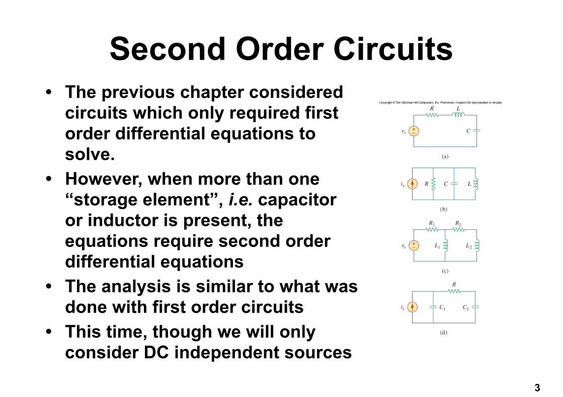
Second Order Circuits• The previous chapter considered

circuits which only required first order differential equations to solve.

• However, when more than one “storage element”, i.e. capacitor or inductor is present, the equations require second order differential equations

• The analysis is similar to what was done with first order circuits

• This time, though we will only consider DC independent sources

!3

Finding Initial and Final Values• Working on second order system is harder

than first order in terms of finding initial and final conditions.

• You need to know the derivatives, dv/dt and di/dt as well.

• Getting the polarity across a capacitor and the direction of current through an inductor is critical.

• Capacitor voltage and inductor current are always continuous.

!4

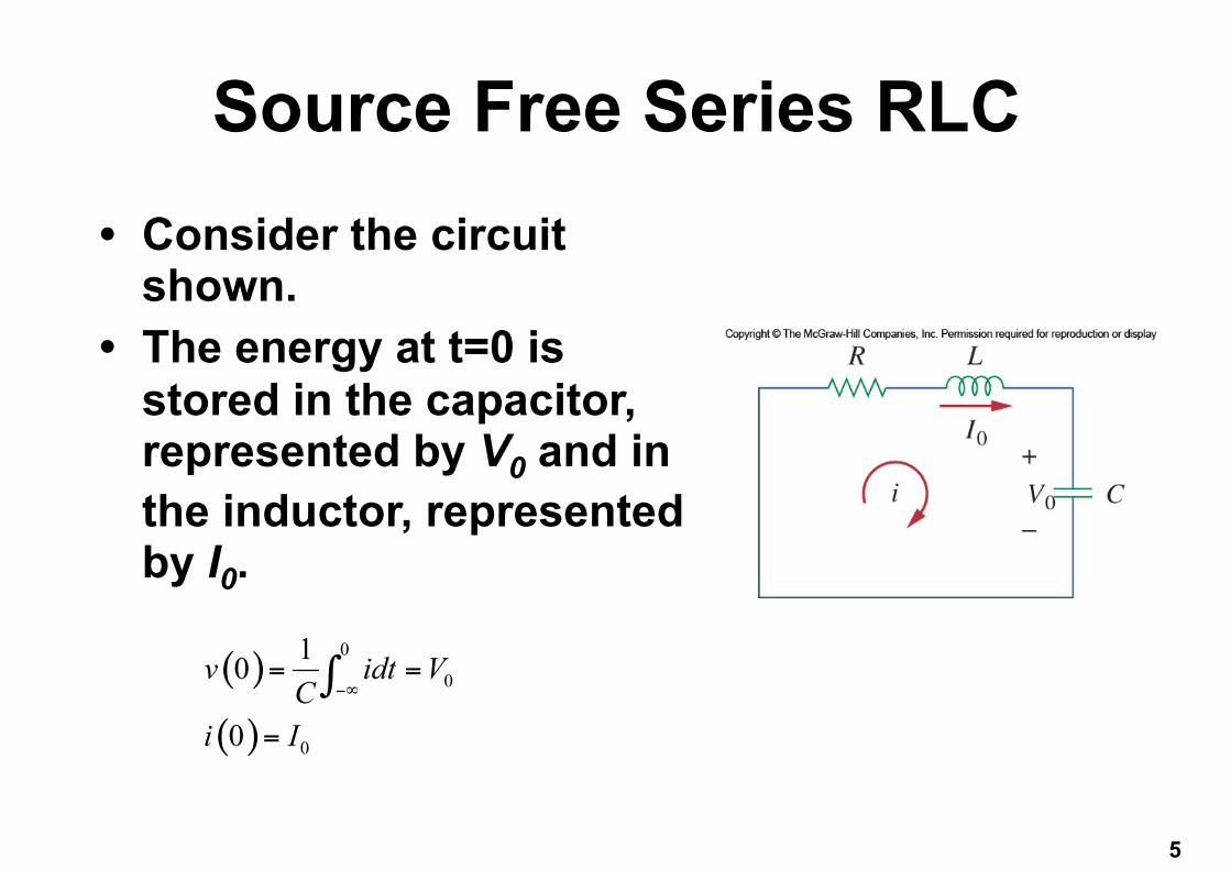
Source Free Series RLC• Consider the circuit

shown. • The energy at t=0 is

stored in the capacitor, represented by V0 and in the inductor, represented by I0.

!5

( )

( )

0

0

0

10

0

v idt VC

i I−∞

= =

=

∫

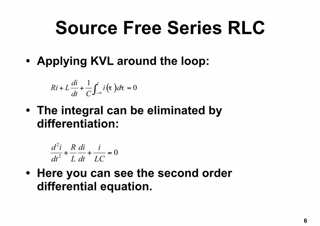
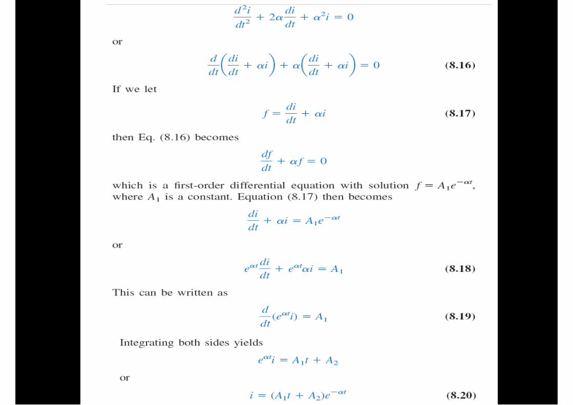
Source Free Series RLC• Applying KVL around the loop:

• The integral can be eliminated by differentiation:

• Here you can see the second order differential equation.

!6

( )1 0tdiRi L i d

dt Cτ τ

−∞+ + =∫

2

2 0d i R di idt L dt LC

+ + =

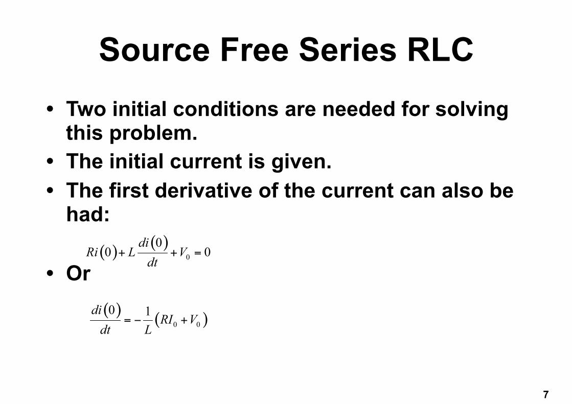
Source Free Series RLC• Two initial conditions are needed for solving

this problem. • The initial current is given. • The first derivative of the current can also be

had:

• Or

!7

( ) ( )0

00 0

diRi L V

dt+ + =

( ) ( )0 0

0 1diRI V

dt L= − +

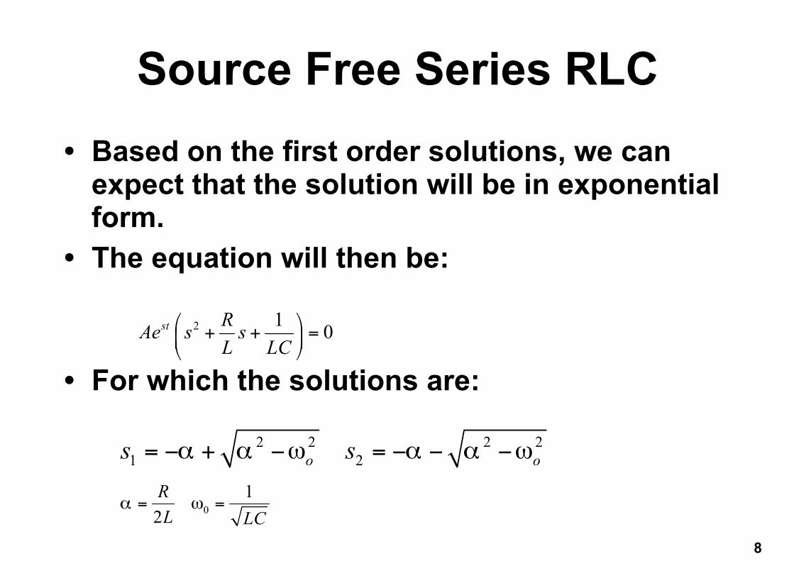
Source Free Series RLC• Based on the first order solutions, we can

expect that the solution will be in exponential form.

• The equation will then be:

• For which the solutions are:

!8

2 1 0st RAe s sL LC

⎛ ⎞+ + =⎜ ⎟⎝ ⎠

2 2 2 21 2o os sα α ω α α ω= − + − = − − −

01

2RL LC

α ω= =

Source Free Series RLC

!9

2

2 0d i R di idt L dt LC

+ + =

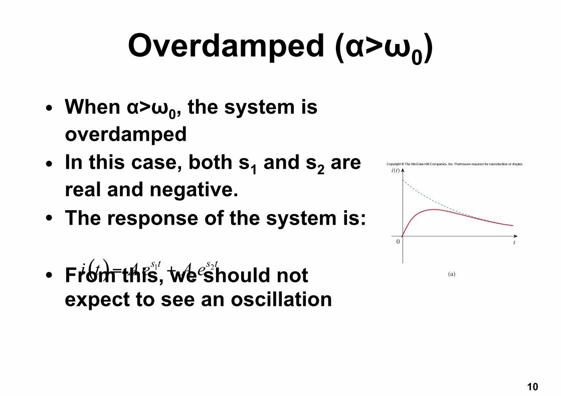
Overdamped (α>ω0)

• When α>ω0, the system is overdamped

• In this case, both s1 and s2 are real and negative.

• The response of the system is:

• From this, we should not expect to see an oscillation

!10

( ) 1 21 2s t s ti t A e A e= +

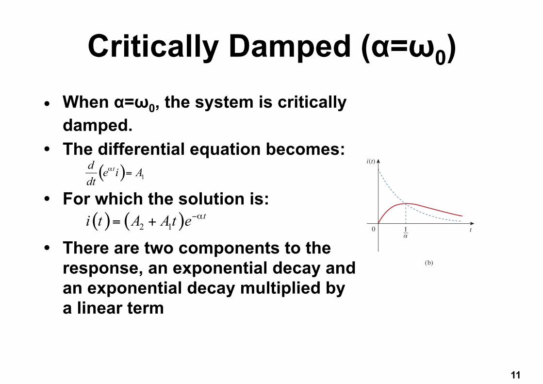
Critically Damped (α=ω0)• When α=ω0, the system is critically

damped. • The differential equation becomes:

• For which the solution is:

• There are two components to the response, an exponential decay and an exponential decay multiplied by a linear term

!11

( ) 1td e i A

dtα =

( ) ( )2 1ti t A A t e α−= +

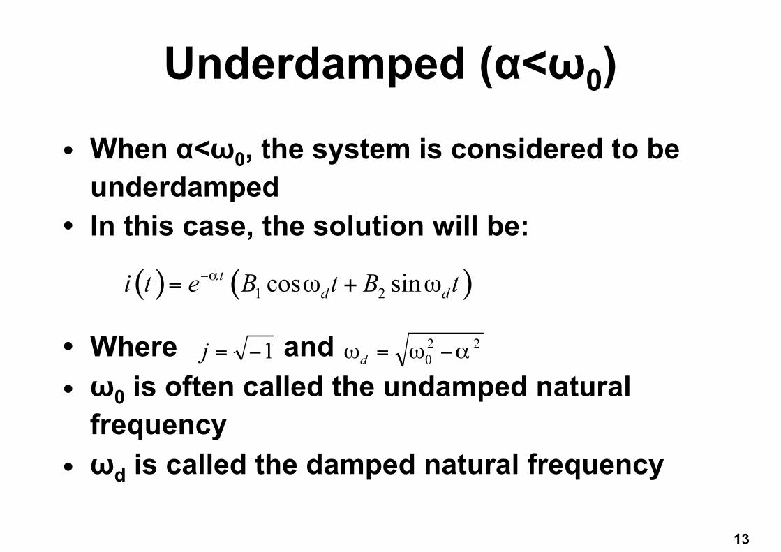
Underdamped (α<ω0)

• When α<ω0, the system is considered to be underdamped

• In this case, the solution will be:

• Where and • ω0 is often called the undamped natural

frequency • ωd is called the damped natural frequency

!13

1−=j 220 αωω −=d

( ) ( )1 2cos sintd di t e B t B tα ω ω−= +

Damping and RLC networks• RLC networks can be charaterized by the

following: 1.The behavior of these networks is captured

by the idea of damping 2.Oscillatory response is possible due to the

presence of two types of energy storage elements.

3. It is typically difficult to tell the difference between damped and critically damped responses.

!14

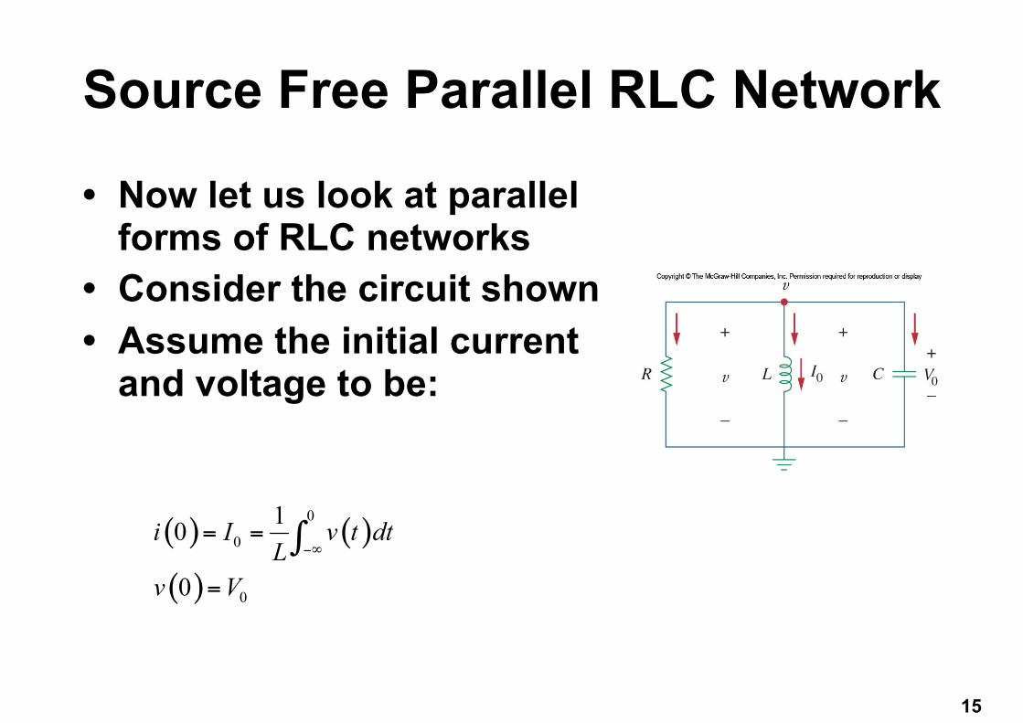
Source Free Parallel RLC Network

• Now let us look at parallel forms of RLC networks

• Consider the circuit shown • Assume the initial current

and voltage to be:

!15

( ) ( )

( )

0

0

0

10

0

i I v t dtL

v V−∞

= =

=

∫

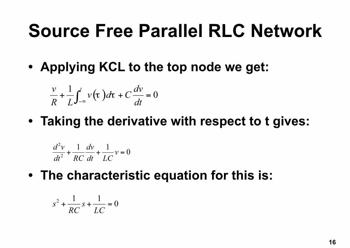
Source Free Parallel RLC Network

• Applying KCL to the top node we get:

• Taking the derivative with respect to t gives:

• The characteristic equation for this is:

!16

( )1 0tv dvv d C

R L dtτ τ

−∞+ + =∫

2

2

1 1 0d v dv vdt RC dt LC

+ + =

2 1 1 0s sRC LC

+ + =

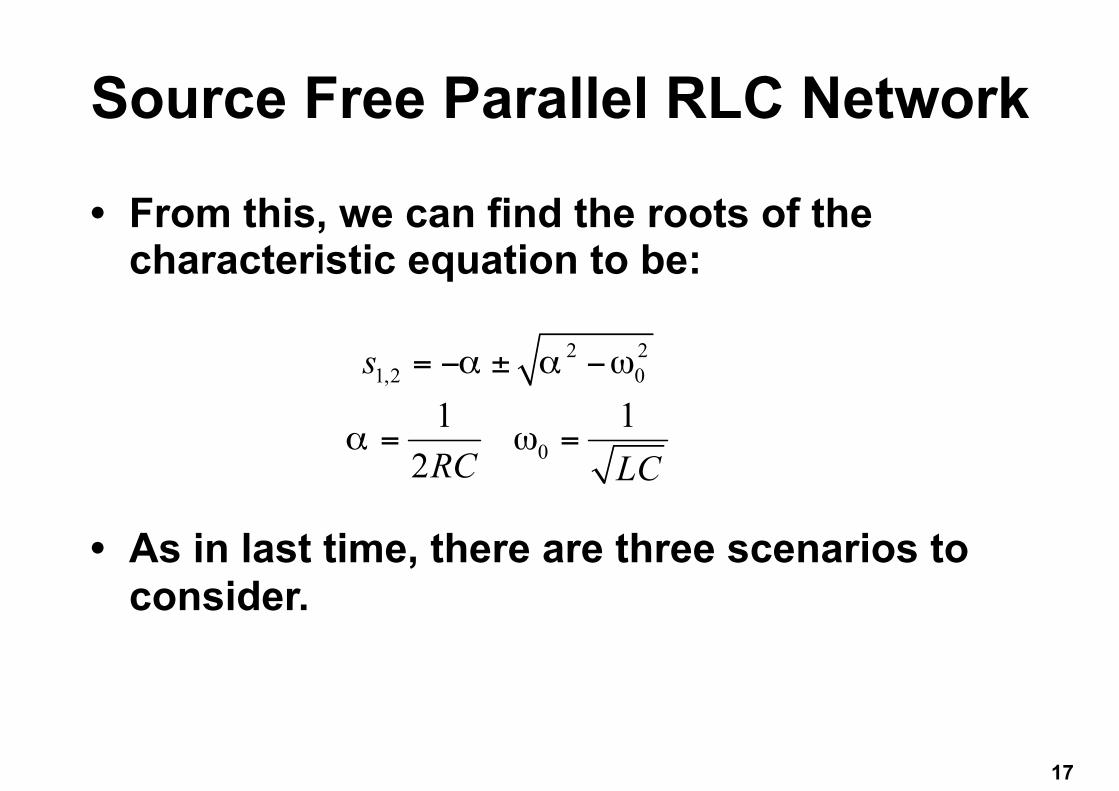
Source Free Parallel RLC Network

• From this, we can find the roots of the characteristic equation to be:

• As in last time, there are three scenarios to consider.

!17

2 21,2 0

01 12

s

RC LC

α α ω

α ω

= − ± −

= =

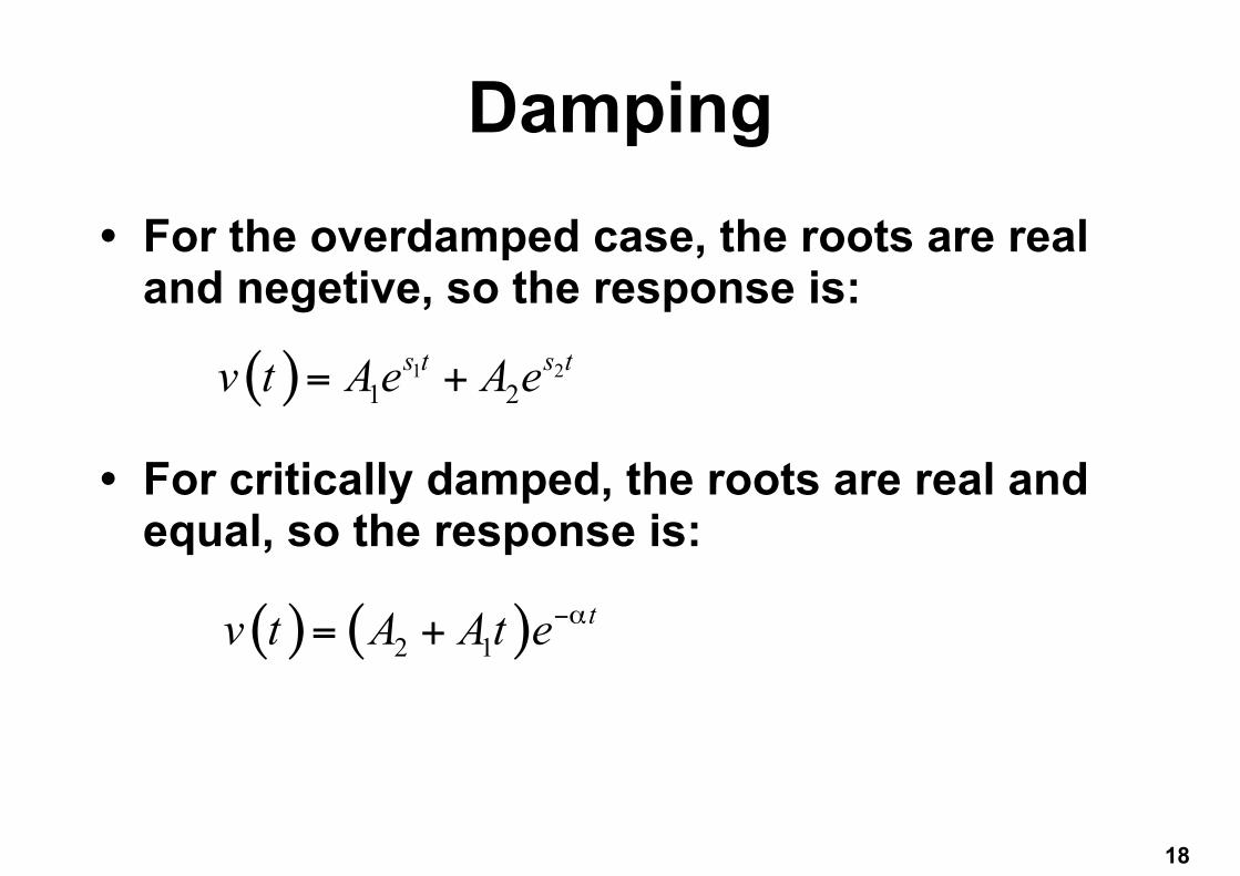
Damping• For the overdamped case, the roots are real

and negetive, so the response is:

• For critically damped, the roots are real and equal, so the response is:

!18

( ) 1 21 2s t s tv t A e A e= +

( ) ( )2 1tv t A At e α−= +

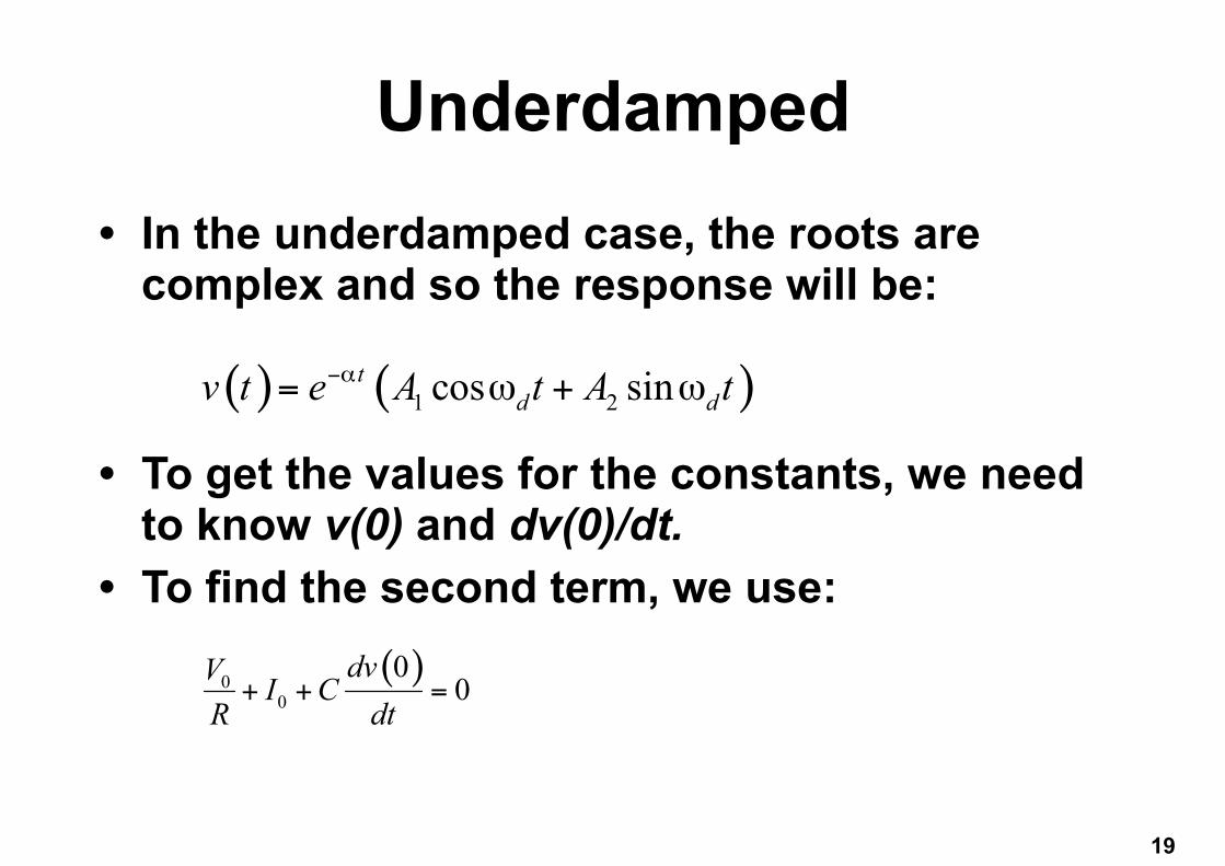
Underdamped• In the underdamped case, the roots are

complex and so the response will be:

• To get the values for the constants, we need to know v(0) and dv(0)/dt.

• To find the second term, we use:

!19

( ) ( )1 2cos sintd dv t e A t A tα ω ω−= +

( )00

00

dvV I CR dt+ + =

Underdamped• The voltage waveforms will be similar to

those shown for the series network. • Note that in the series network, we first found

the inductor current and then solved for the rest from that.

• Here we start with the capacitor voltage and similarly, solve for the other variables from that.

!20

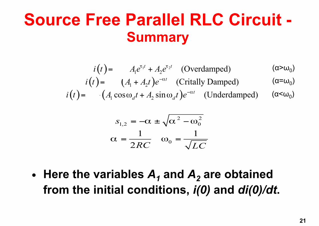
Source Free Parallel RLC Circuit - Summary

• Here the variables A1 and A2 are obtained from the initial conditions, i(0) and di(0)/dt.

!21

( )( ) ( )

( ) ( )

1 21 2

1 2

1 2

(Overdamped)(Critally Damped)

cos sin (Underdamped)

t ts

ts

ts d d

i t I A e A ei t I A A t e

i t I A t A t e

τ τ

α

αω ω

−

−

= + +

= + +

= + +

2 21,2 0

01 12

s

RC LC

α α ω

α ω

= − ± −

= =

(α>ω0)

(α=ω0)

(α<ω0)

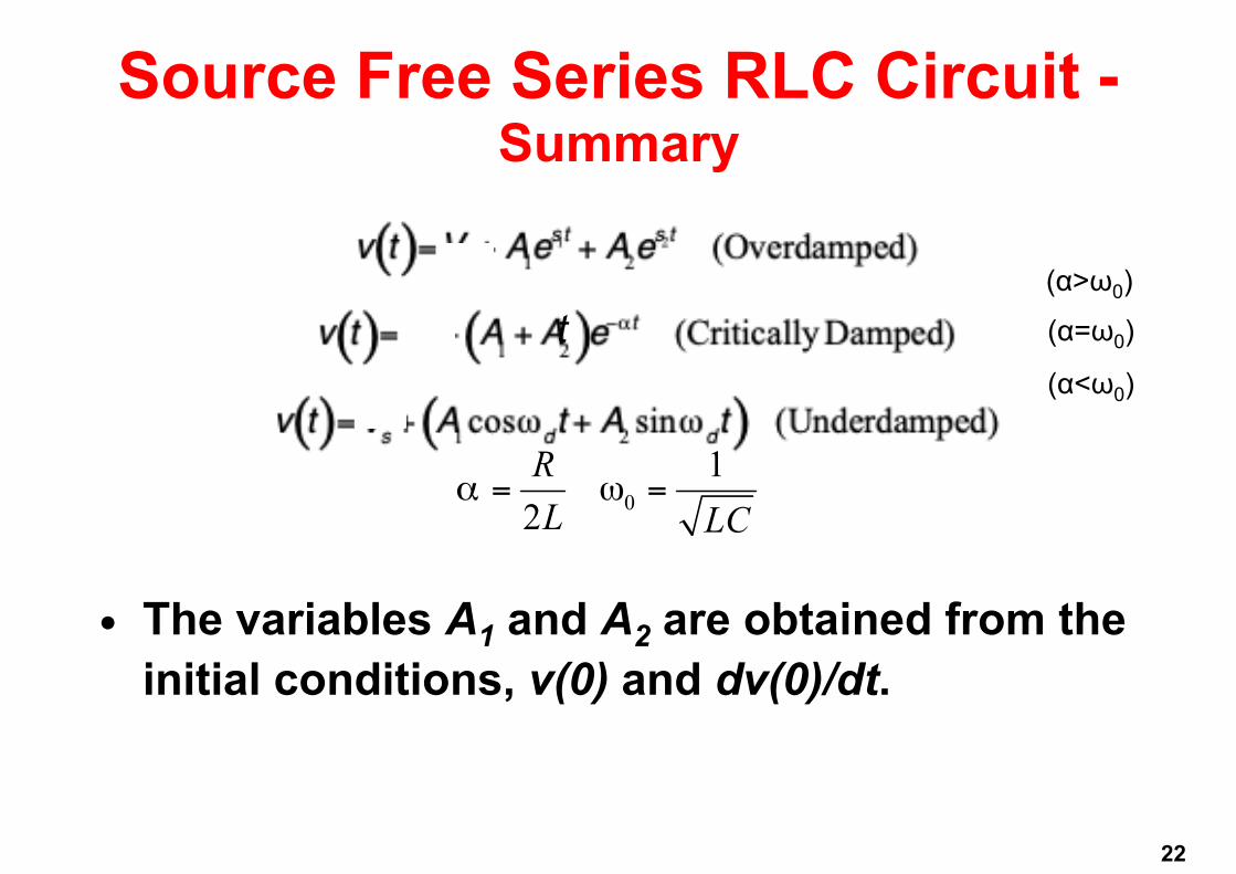
Source Free Series RLC Circuit - Summary

• The variables A1 and A2 are obtained from the initial conditions, v(0) and dv(0)/dt.

!22

01

2RL LC

α ω= =

(α>ω0)

(α=ω0)

(α<ω0)

t

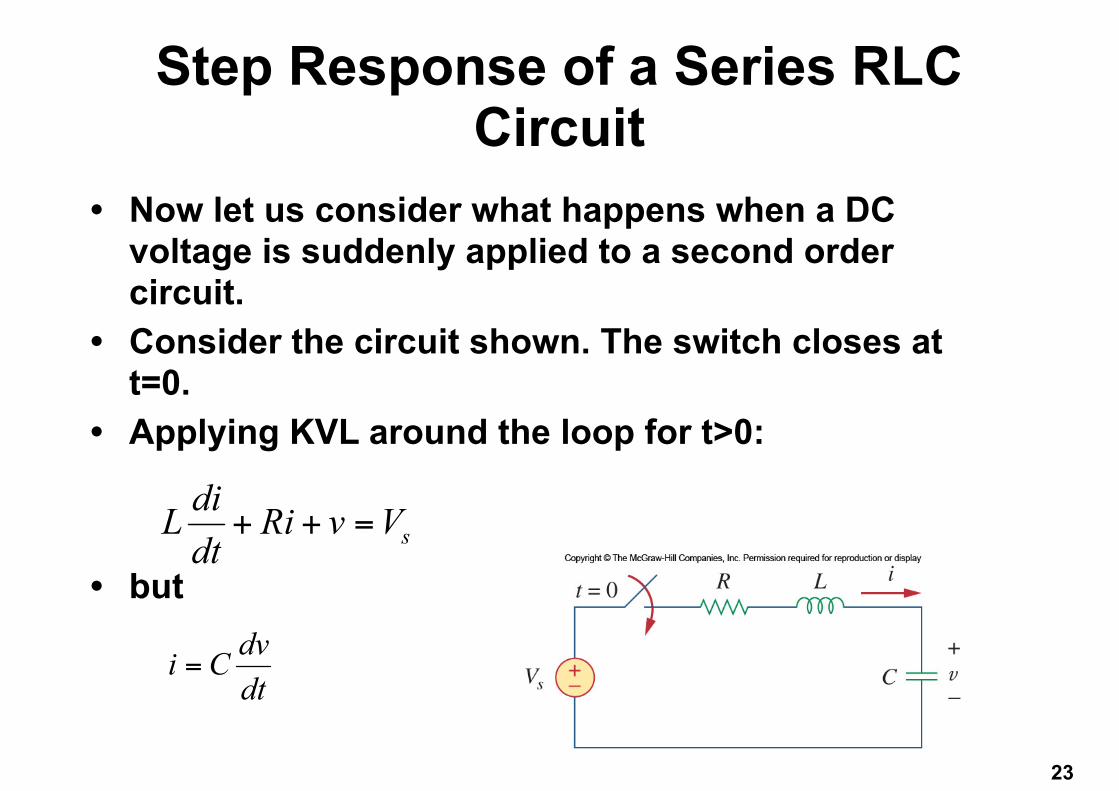
Step Response of a Series RLC Circuit

• Now let us consider what happens when a DC voltage is suddenly applied to a second order circuit.

• Consider the circuit shown. The switch closes at t=0.

• Applying KVL around the loop for t>0:

• but

!23

sdiL Ri v Vdt+ + =

dvi Cdt

=

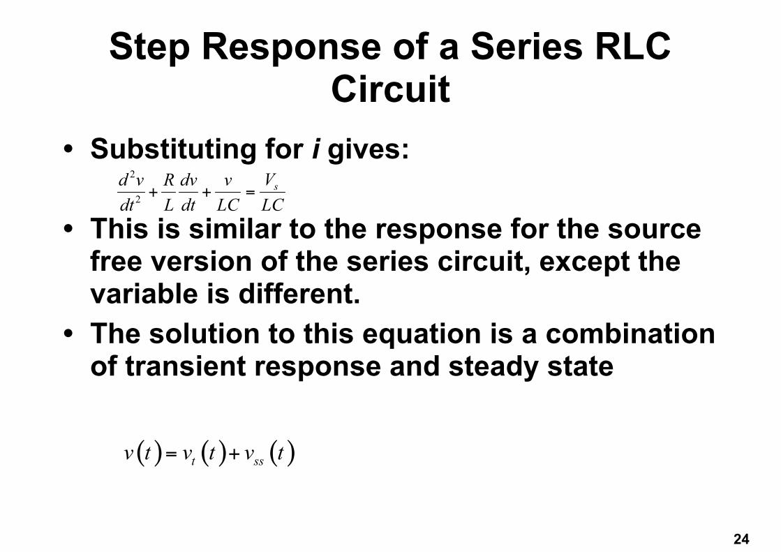
Step Response of a Series RLC Circuit

• Substituting for i gives:

• This is similar to the response for the source free version of the series circuit, except the variable is different.

• The solution to this equation is a combination of transient response and steady state

!24

2

2sVd v R dv v

dt L dt LC LC+ + =

( ) ( ) ( )t ssv t v t v t= +

Step Response of a Series RLC Circuit

• The transient response is in the same form as the solutions for the source free version.

• The steady state response is the final value of v(t). In this case, the capacitor voltage will equal the source voltage.

!25

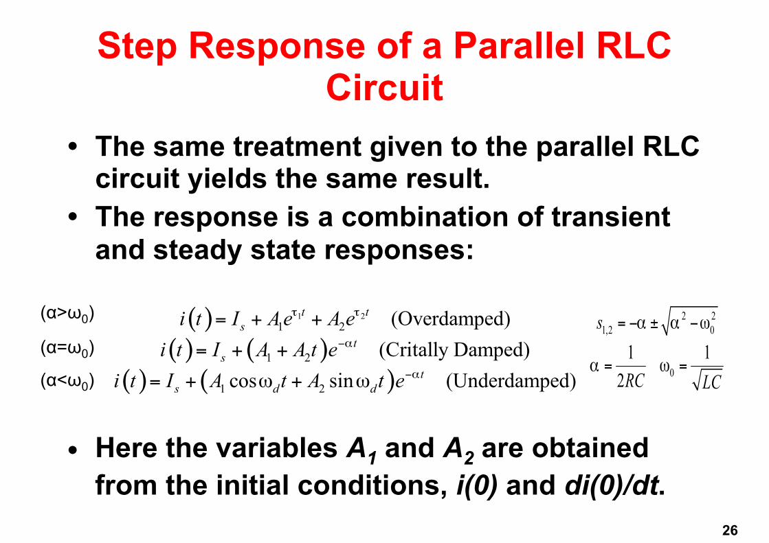
Step Response of a Parallel RLC Circuit

• The same treatment given to the parallel RLC circuit yields the same result.

• The response is a combination of transient and steady state responses:

• Here the variables A1 and A2 are obtained from the initial conditions, i(0) and di(0)/dt.

!26

( )( ) ( )

( ) ( )

1 21 2

1 2

1 2

(Overdamped)(Critally Damped)

cos sin (Underdamped)

t ts

ts

ts d d

i t I A e A ei t I A A t e

i t I A t A t e

τ τ

α

αω ω

−

−

= + +

= + +

= + +

2 21,2 0

01 12

s

RC LC

α α ω

α ω

= − ± −

= =

(α>ω0)

(α=ω0)

(α<ω0)

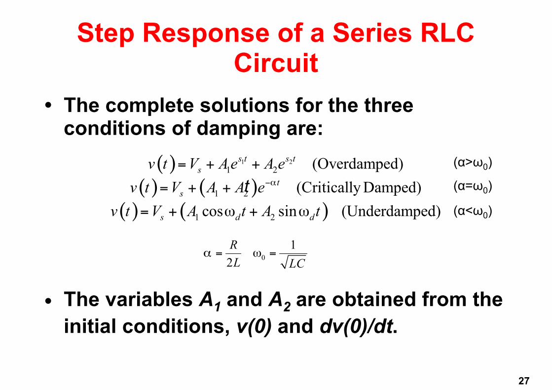
Step Response of a Series RLC Circuit

• The complete solutions for the three conditions of damping are:

• The variables A1 and A2 are obtained from the initial conditions, v(0) and dv(0)/dt.

!27

( )( ) ( )

( ) ( )

1 21 2

1 2

1 2

(Overdamped)(CriticallyDamped)

cos sin (Underdamped)

s t s ts

ts

s d d

v t V Ae A ev t V A A e

v t V A t A t

α

ω ω

−

= + +

= + +

= + +

01

2RL LC

α ω= =

(α>ω0)

(α=ω0)

(α<ω0)

t

General Second Order Circuits• The principles of the approach to solving the

series and parallel forms of RLC circuits can be applied to second order circuits in general:

• The following four steps need to be taken: 1.First determine the initial conditions, x(0) and

dx(0)/dt.

!28

Second Order Op-amp Circuits2. Turn off the independent sources and find

the form of the transient response by applying KVL and KCL.

• Depending on the damping found, the unknown constants will be found.

3. We obtain the stead state response as:

Where x(∞) is the final value of x obtained in step 1

!29

( ) ( )ssx t x= ∞

Second Order Op-amp Circuits II

4. The total response is now found as the sum of the transient response and steady-state response.

!30

( ) ( ) ( )t ssx t x t x t= +

Duality• The concept of duality is a time saving

measure for solving circuit problems. • It is based on the idea that circuits that

appear to be different may be related to each other.

• They may use the same equations, but the roles of certain complimentary elements are interchanged.

• The following is a table of dual pairs

!31

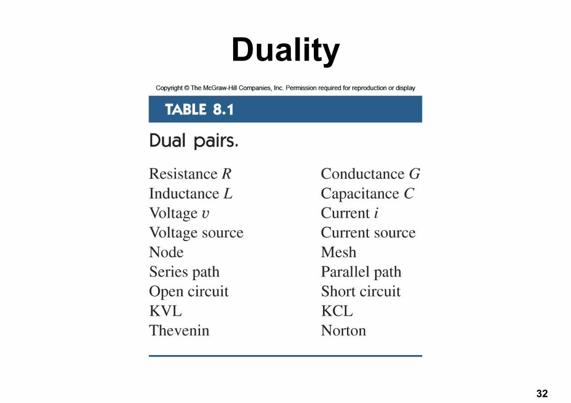
Duality

!32

Duality• Once you know the solution to one circuit,

you have the solution to the dual circuit. • Finding the dual of a circuit can be done with

a graphical method: 1.Place a node at the center of each mesh of a

given circuit. Place the reference node outside the given circuit.

2.Draw lines between the nodes such that each line crosses an element. Replace the element with its dual

!33

Duality3. To determine the polarity of voltage sources

and of current sources, follow this rule: A voltage source that produces a positive (clockwise) mesh current has as its dual a current source whose reference direction is from the ground to the nonreference node.

• When in doubt, one can refer to the mesh or nodal equations of the dual circuit.

!34