table of contents · laboratory manual 204 fundamentals of electrical circuits 2 preface the ee...
TRANSCRIPT
Laboratory Manual 204 Fundamentals of Electrical Circuits
1
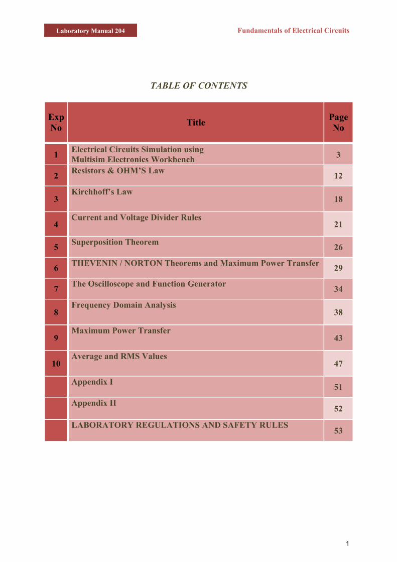
TABLE OF CONTENTS
Exp No Title Page
No
1 Electrical Circuits Simulation using Multisim Electronics Workbench 3
2 Resistors & OHM’S Law 12
3 Kirchhoff’s Law
18
4 Current and Voltage Divider Rules
21
5 Superposition Theorem 26
6 THEVENIN / NORTON Theorems and Maximum Power Transfer 29
7 The Oscilloscope and Function Generator 34
8 Frequency Domain Analysis
38
9 Maximum Power Transfer
43
10 Average and RMS Values
47
Appendix I 51
Appendix II
52
LABORATORY REGULATIONS AND SAFETY RULES 53
Laboratory Manual 204 Fundamentals of Electrical Circuits
2
PREFACE
The EE 204: Fundamentals of Electric Circuits Lab is intended to teach the basics of Electrical Engineering to undergraduates of other engineering departments. The main aim is to provide hands-on experience to the students so that they are able to put theoretical concepts to practice. The manual starts off with the basic laws such as Ohm's Law and Kirchhoff's Current and Voltage Laws. The two experiments augment students' understanding of the relations of voltage and current how they are implemented in practical life. Computer simulation is also stressed upon as it is a key analysis tool of engineering design. Multisim is used for simulation of electric circuits and is a standard tool at numerous universities and industries of the world. The simulated parameters are then verified through actual experiment. Use of oscilloscopes is also stressed upon as analysis tool. The important theorems of Thevenin and Norton are also provided along with the frequency domain analysis of circuits. They greatly simplify the complex electrical networks for analysis purposes. At the end, the students should be able to grasp the concepts thoroughly the electric circuits and able to apply them further in their field of study.
Laboratory Manual 204 Fundamentals of Electrical Circuits
3
Experiment No. 1
Electrical Circuits Simulation using Multisim Electronics Workbench: An Introduction
Simulation is a mathematical way of representing the actual behavior of a circuit. With simulation, you can determine a circuit’s performance without physically constructing the circuit or using actual test instruments. Multisim is a complete system design tool that offers a very large component database, schematic entry, full analog/digital SPICE simulation, etc. It also offers a single easy to use graphical interface for all design needs.
Introduction
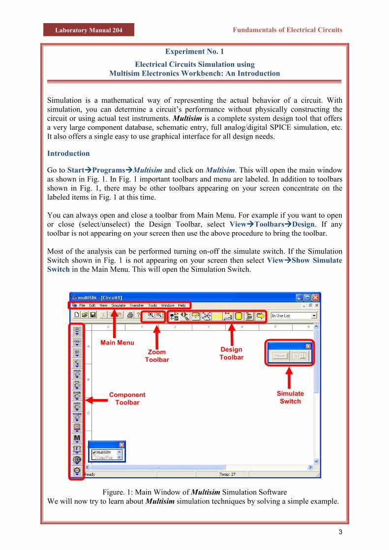
Go to StartààààProgramsààààMultisim and click on Multisim. This will open the main window as shown in Fig. 1. In Fig. 1 important toolbars and menu are labeled. In addition to toolbars shown in Fig. 1, there may be other toolbars appearing on your screen concentrate on the labeled items in Fig. 1 at this time. You can always open and close a toolbar from Main Menu. For example if you want to open or close (select/unselect) the Design Toolbar, select ViewààààToolbarsààààDesign. If any toolbar is not appearing on your screen then use the above procedure to bring the toolbar. Most of the analysis can be performed turning on-off the simulate switch. If the Simulation Switch shown in Fig. 1 is not appearing on your screen then select ViewààààShow Simulate Switch in the Main Menu. This will open the Simulation Switch.
Figure. 1: Main Window of Multisim Simulation Software We will now try to learn about Multisim simulation techniques by solving a simple example.
Design Toolbar
Main Menu
Simulate Switch
Component Toolbar
Zoom Toolbar
Laboratory Manual 204 Fundamentals of Electrical Circuits
4
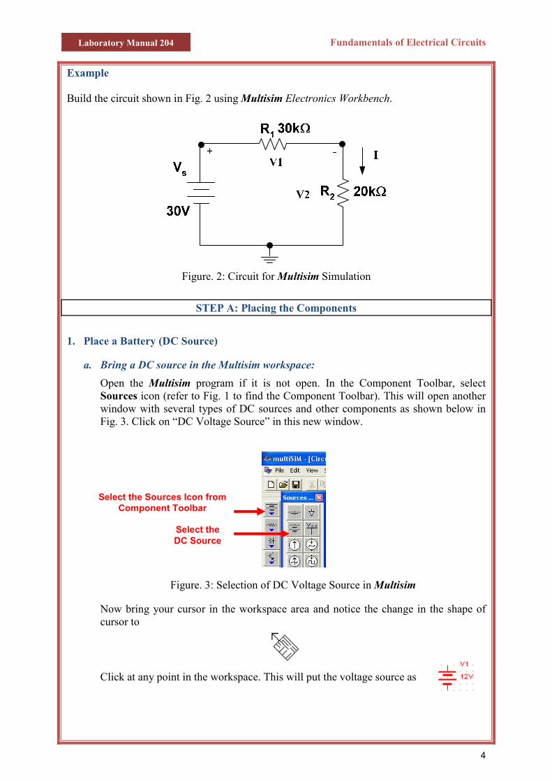
Example Build the circuit shown in Fig. 2 using Multisim Electronics Workbench.
Figure. 2: Circuit for Multisim Simulation
STEP A: Placing the Components
1. Place a Battery (DC Source)
a. Bring a DC source in the Multisim workspace:
Open the Multisim program if it is not open. In the Component Toolbar, select Sources icon (refer to Fig. 1 to find the Component Toolbar). This will open another window with several types of DC sources and other components as shown below in Fig. 3. Click on “DC Voltage Source” in this new window.
Figure. 3: Selection of DC Voltage Source in Multisim
Now bring your cursor in the workspace area and notice the change in the shape of cursor to
Click at any point in the workspace. This will put the voltage source as
Select the Sources Icon from Component Toolbar
Select the DC Source
Laboratory Manual 204 Fundamentals of Electrical Circuits
5
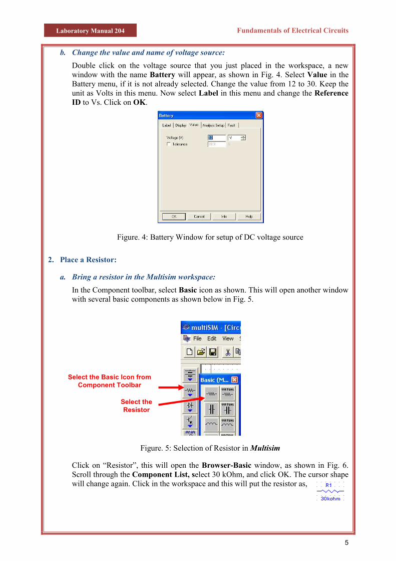
b. Change the value and name of voltage source:
Double click on the voltage source that you just placed in the workspace, a new window with the name Battery will appear, as shown in Fig. 4. Select Value in the Battery menu, if it is not already selected. Change the value from 12 to 30. Keep the unit as Volts in this menu. Now select Label in this menu and change the Reference ID to Vs. Click on OK.
Figure. 4: Battery Window for setup of DC voltage source
2. Place a Resistor:
a. Bring a resistor in the Multisim workspace:
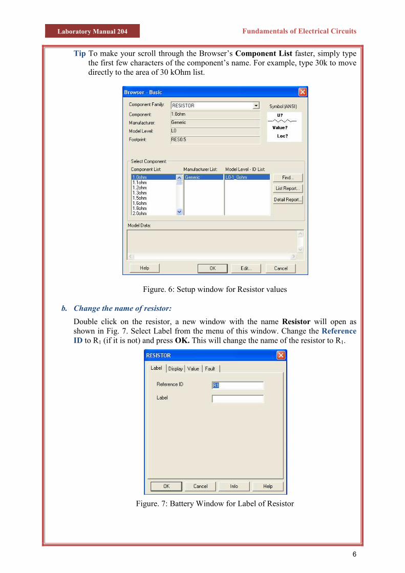
In the Component toolbar, select Basic icon as shown. This will open another window with several basic components as shown below in Fig. 5.
Figure. 5: Selection of Resistor in Multisim
Click on “Resistor”, this will open the Browser-Basic window, as shown in Fig. 6. Scroll through the Component List, select 30 kOhm, and click OK. The cursor shape will change again. Click in the workspace and this will put the resistor as,
Select the Basic Icon from Component Toolbar
Select the Resistor
Laboratory Manual 204 Fundamentals of Electrical Circuits
6
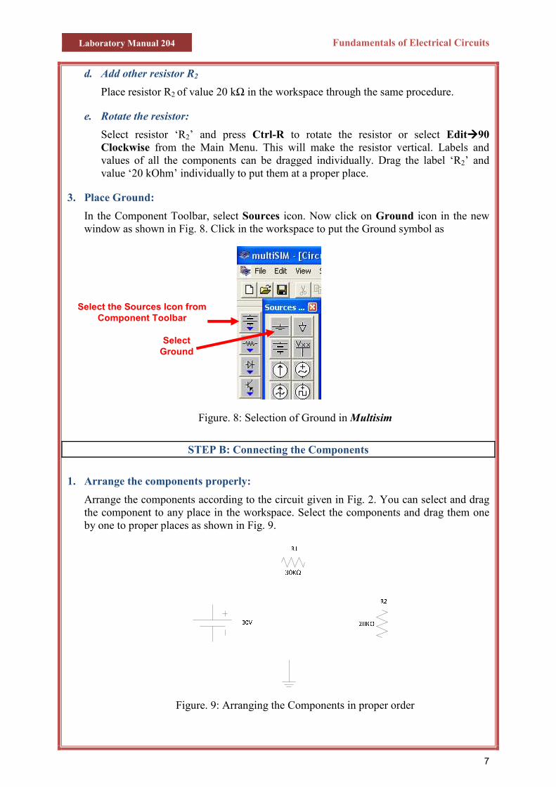
Tip To make your scroll through the Browser’s Component List faster, simply type the first few characters of the component’s name. For example, type 30k to move directly to the area of 30 kOhm list.
Figure. 6: Setup window for Resistor values
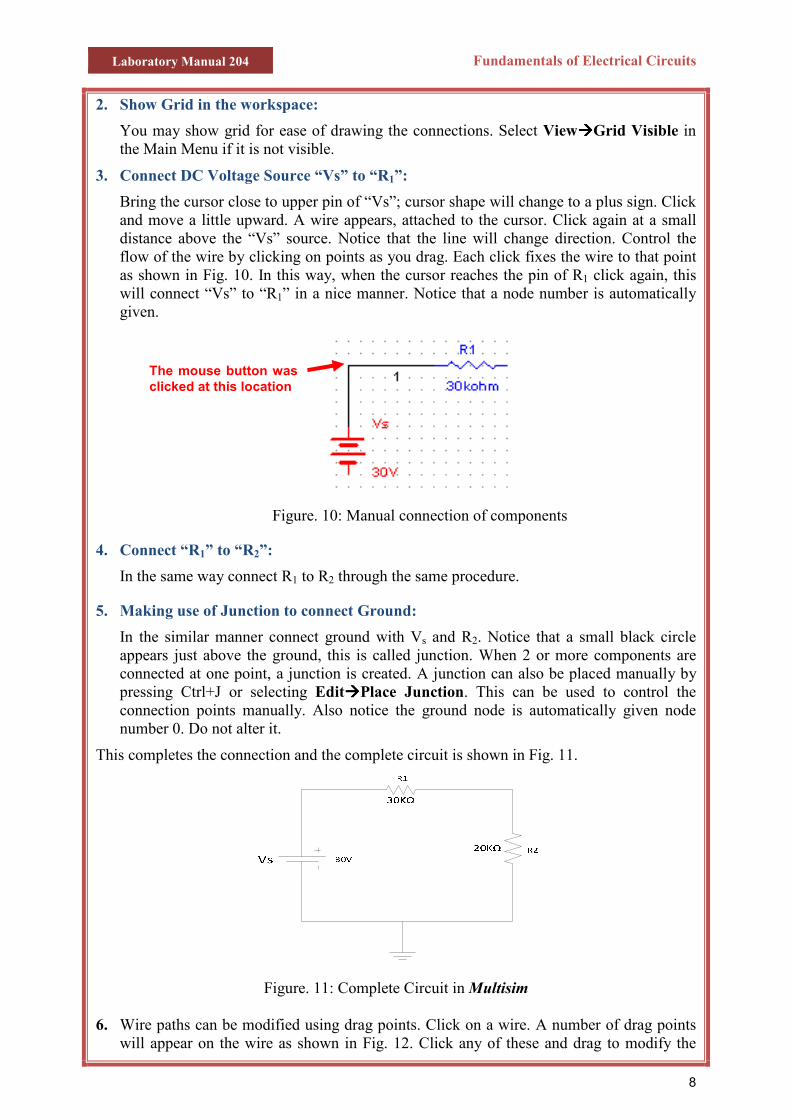
b. Change the name of resistor:
Double click on the resistor, a new window with the name Resistor will open as shown in Fig. 7. Select Label from the menu of this window. Change the Reference ID to R1 (if it is not) and press OK. This will change the name of the resistor to R1.
Figure. 7: Battery Window for Label of Resistor
Laboratory Manual 204 Fundamentals of Electrical Circuits
d. Add other resistor R2
Place resistor R2 of value 20 kΩ in the workspace through the same procedure.
e. Rotate the resistor:
Select resistor ‘R2’ and press Ctrl-R to rotate the resistor or select Editàààà90 Clockwise from the Main Menu. This will make the resistor vertical. Labels and values of all the components can be dragged individually. Drag the label ‘R2’ and value ‘20 kOhm’ individually to put them at a proper place.
3. Place Ground:
In the Component Toolbar, select Sources icon. Now click on Ground icon in the new window as shown in Fig. 8. Click in the workspace to put the Ground symbol as
Figure. 8: Selection of Ground in Multisim
STEP B: Connecting the Components
1. Arrange the components properly:
Arrange the components according to the circuit given in Fig. 2. You can select and drag the component to any place in the workspace. Select the components and drag them one by one to proper places as shown in Fig. 9.
Figure. 9: Arrangi
Select Ground
Select the Sources Icon from Component Toolbar
7
ng the Components in proper order
Laboratory Manual 204 Fundamentals of Electrical Circuits
8
2. Show Grid in the workspace:
You may show grid for ease of drawing the connections. Select ViewààààGrid Visible in the Main Menu if it is not visible.
3. Connect DC Voltage Source “Vs” to “R1”:
Bring the cursor close to upper pin of “Vs”; cursor shape will change to a plus sign. Click and move a little upward. A wire appears, attached to the cursor. Click again at a small distance above the “Vs” source. Notice that the line will change direction. Control the flow of the wire by clicking on points as you drag. Each click fixes the wire to that point as shown in Fig. 10. In this way, when the cursor reaches the pin of R1 click again, this will connect “Vs” to “R1” in a nice manner. Notice that a node number is automatically given.
Figure. 10: Manual connection of components
4. Connect “R1” to “R2”:
In the same way connect R1 to R2 through the same procedure.
5. Making use of Junction to connect Ground:
In the similar manner connect ground with Vs and R2. Notice that a small black circle appears just above the ground, this is called junction. When 2 or more components are connected at one point, a junction is created. A junction can also be placed manually by pressing Ctrl+J or selecting EditààààPlace Junction. This can be used to control the connection points manually. Also notice the ground node is automatically given node number 0. Do not alter it.
This completes the connection and the complete circuit is shown in Fig. 11.
Figure. 11: Complete Circuit in Multisim
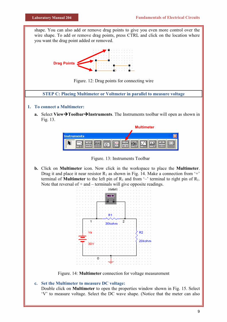
6. Wire paths can be modified using drag points. Click on a wire. A number of drag points will appear on the wire as shown in Fig. 12. Click any of these and drag to modify the
The mouse button was clicked at this location
Laboratory Manual 204 Fundamentals of Electrical Circuits
shape. You can also add or remove drag points to give you even more control over the wire shape. To add or remove drag points, press CTRL and click on the location where you want the drag point added or removed.
Figure. 12: Drag points for connecting wire
STEP C: Placing Multimeter or Voltmeter in parallel to measure voltage
1. To connect a Multimeter:
a. Select ViewààààToolbarààààInstruments. The Instruments toolbar will open as shown in Fig. 13.
Figure. 13: Instruments Tool
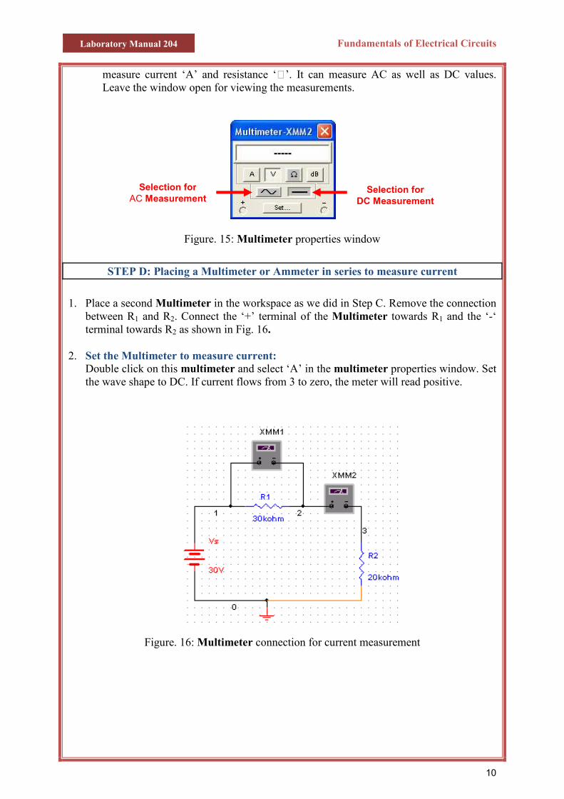
b. Click on Multimeter icon. Now click in the workspaDrag it and place it near resistor R1 as shown in Fig. 14terminal of Multimeter to the left pin of R1 and from ‘Note that reversal of + and – terminals will give opposit
Figure. 14: Multimeter connection for voltage
c. Set the Multimeter to measure DC voltage: Double click on Multimeter to open the properties win‘V’ to measure voltage. Select the DC wave shape. (N
Drag Points
Multi
meter9
bar
ce to place the Multimeter. . Make a connection from ‘+’ –’ terminal to right pin of R1. e readings.
measurement
dow shown in Fig. 15. Select otice that the meter can also
Laboratory Manual 204 Fundamentals of Electrical Circuits
10
measure current ‘A’ and resistance ‘K’. It can measure AC as well as DC values. Leave the window open for viewing the measurements.
Figure. 15: Multimeter properties window
STEP D: Placing a Multimeter or Ammeter in series to measure current
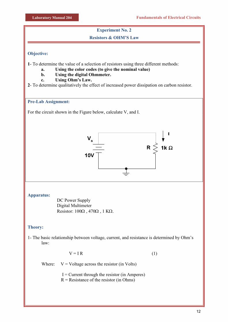
1. Place a second Multimeter in the workspace as we did in Step C. Remove the connection between R1 and R2. Connect the ‘+’ terminal of the Multimeter towards R1 and the ‘-‘ terminal towards R2 as shown in Fig. 16.
2. Set the Multimeter to measure current: Double click on this multimeter and select ‘A’ in the multimeter properties window. Set the wave shape to DC. If current flows from 3 to zero, the meter will read positive.
Figure. 16: Multimeter connection for current measurement
Selection for DC Measurement
Selection for AC Measurement

Laboratory Manual 204 Fundamentals of Electrical Circuits
11
NAME ______________________ SEC # __________ ID # ______________________ SERIAL# __________
Example: V1 V2 IT
Exercise: IT I1 I2 V1 V2
Conclusion:
Laboratory Manual 204 Fundamentals of Electrical Circuits
12
Experiment No. 2
Resistors & OHM’S Law Objective:
1- To determine the value of a selection of resistors using three different methods:
a. Using the color codes (to give the nominal value) b. Using the digital Ohmmeter. c. Using Ohm’s Law.
2- To determine qualitatively the effect of increased power dissipation on carbon resistor.
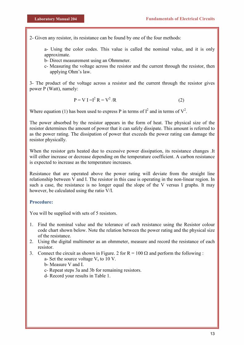
Pre-Lab Assignment: For the circuit shown in the Figure below, calculate V, and I.
Apparatus: DC Power Supply Digital Multimeter
Resistor: 100Ω , 470Ω , 1 KΩ.
Theory:
1- The basic relationship between voltage, current, and resistance is determined by Ohm’s
law:
V = I R (1)
Where: V = Voltage across the resistor (in Volts)
I = Current through the resistor (in Amperes) R = Resistance of the resistor (in Ohms)
Laboratory Manual 204 Fundamentals of Electrical Circuits
13
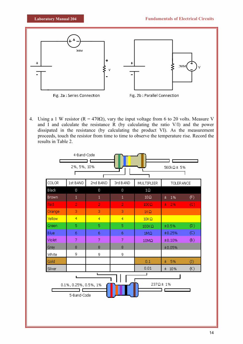
2- Given any resistor, its resistance can be found by one of the four methods:
a- Using the color codes. This value is called the nominal value, and it is only approximate. b- Direct measurement using an Ohmmeter. c- Measuring the voltage across the resistor and the current through the resistor, then
applying Ohm’s law. 3- The product of the voltage across a resistor and the current through the resistor gives power P (Watt), namely: P = V I =I2 R = V2 /R (2) Where equation (1) has been used to express P in terms of I2 and in terms of V2. The power absorbed by the resistor appears in the form of heat. The physical size of the resistor determines the amount of power that it can safely dissipate. This amount is referred to as the power rating. The dissipation of power that exceeds the power rating can damage the resistor physically. When the resistor gets heated due to excessive power dissipation, its resistance changes .It will either increase or decrease depending on the temperature coefficient. A carbon resistance is expected to increase as the temperature increases. Resistance that are operated above the power rating will deviate from the straight line relationship between V and I. The resistor in this case is operating in the non-linear region. In such a case, the resistance is no longer equal the slope of the V versus I graphs. It may however, be calculated using the ratio V/I. Procedure: You will be supplied with sets of 5 resistors. 1. Find the nominal value and the tolerance of each resistance using the Resistor colour
code chart shown below. Note the relation between the power rating and the physical size of the resistance.
2. Using the digital multimeter as an ohmmeter, measure and record the resistance of each resistor.
3. Connect the circuit as shown in Figure. 2 for R = 100 Ω and perform the following : a- Set the source voltage Vs to 10 V. b- Measure V and I. c- Repeat steps 3a and 3b for remaining resistors. d- Record your results in Table 1.
Laboratory Manual 204 Fundamentals of Electrical Circuits
14
4. Using a 1 W resistor (R = 470Ω), vary the input voltage from 6 to 20 volts. Measure V and I and calculate the resistance R (by calculating the ratio V/I) and the power dissipated in the resistance (by calculating the product VI). As the measurement proceeds, touch the resistor from time to time to observe the temperature rise. Record the results in Table 2.
Laboratory Manual 204 Fundamentals of Electrical Circuits
15
Questions: 1. Plot P versus R in Fig. 3.
R
P
Figure. 3: R versus P
Comment on the linearity of R as P increases. 2. Does the resistor in step 4 operate in the linear region or non-linear region? Explain
by considering the power rating of the resistor. 3. An electric heater takes 1.48 kW from a voltage source of 220 V. Find the resistance
of the heater? 4. If the current in a resistor doubles, what happens to the dissipated power? (Assume
the resistor operates in the linear region). 5. A 4 Ω resistor is needed to be used in circuit where the voltage across the resistor is
3V .If two 4 Ω resistors with 2 W and 3 W power rating are available, which will you use and why?
Laboratory Manual 204 Fundamentals of Electrical Circuits
16
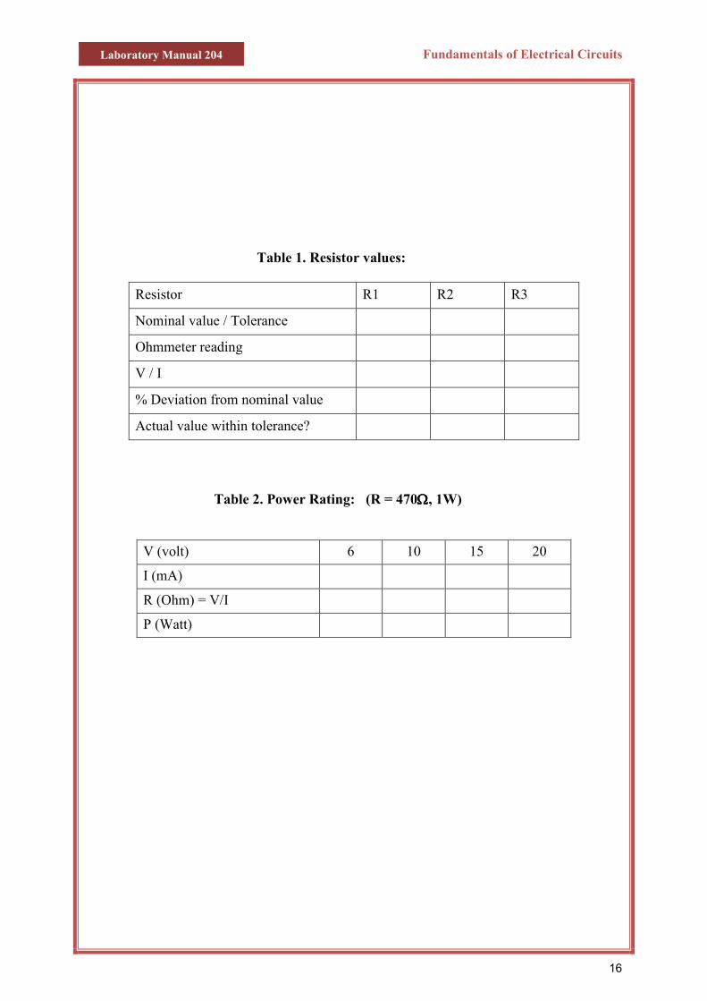
Table 1. Resistor values:
Resistor R1 R2 R3
Nominal value / Tolerance
Ohmmeter reading
V / I
% Deviation from nominal value
Actual value within tolerance?
Table 2. Power Rating: (R = 470ΩΩΩΩ, 1W)
V (volt) 6 10 15 20
I (mA)
R (Ohm) = V/I
P (Watt)
Laboratory Manual 204 Fundamentals of Electrical Circuits
17
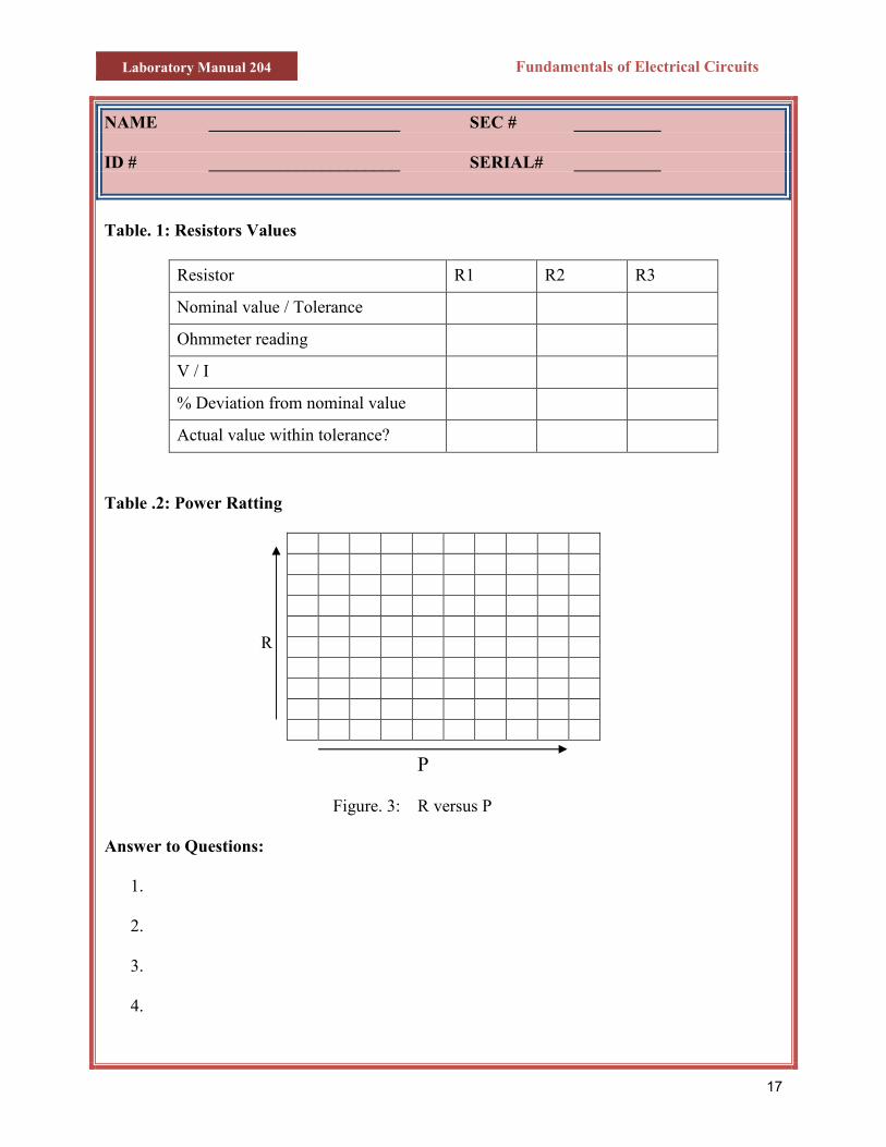
NAME ______________________ SEC # __________ ID # ______________________ SERIAL# __________
Table. 1: Resistors Values
Resistor R1 R2 R3
Nominal value / Tolerance
Ohmmeter reading
V / I
% Deviation from nominal value
Actual value within tolerance?
Table .2: Power Ratting
R
P
Figure. 3: R versus P Answer to Questions:
1.
2.
3.
4.
Laboratory Manual 204 Fundamentals of Electrical Circuits
Experiment No. 3
Kirchhoff’s Law
Objective: To verify Kirchhoff’s Voltage and Current Law experimentally. Apparatus: Theory:
•••• Kirchhoff’s The alge •••• Kirchhoff’s
The alge Procedure:
1- Check the vRecord the v
2- Connect thevoltage Vs to
3- Measure the(including th
4- Measure theTable. 3
Pre-Lab Assi For th
1- VA
2- I1,
gnment:
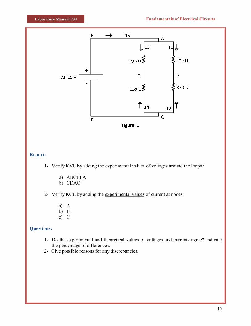
e circuit shown in Figure 1, calculate:
B , VBC , VAD , VDC , VBD , and VAC. I2, I3, I4 and I5.
18
DC Power Supply Digital Multimeter Carbon Resistors: 100Ω, 150Ω, 220Ω, and 330Ω
Voltage Law ( KVL ): braic sum of all voltages around any closed path is equal to zero.
current Law ( KCL ): braic sum of all currents at a junction point is equal to zero.
alues of the resistors, used in the circuit of Figure.1, using a multimeter. alues in Table 1. circuit as shown, and have it checked by the instructor. Adjust the supply 10 V, using a DC voltmeter (DMM). voltages VAB, VBC , VAD , VDC , VBD , and VAC. Record their values e signs) in Table 2 currents I1 , I2 , I3 , I4 and I5 and record their values (including the signs) in
Laboratory Manual 204 Fundamentals of Electrical Circuits
19
Report:
1- Verify KVL by adding the experimental values of voltages around the loops :
a) ABCEFA b) CDAC
2- Verify KCL by adding the experimental values of current at nodes:
a) A b) B c) C
Questions:
1- Do the experimental and theoretical values of voltages and currents agree? Indicate the percentage of differences.
2- Give possible reasons for any discrepancies.
Laboratory Manual 204 Fundamentals of Electrical Circuits
20
NAME ______________________ SEC # __________ ID # ______________________ SERIAL# __________
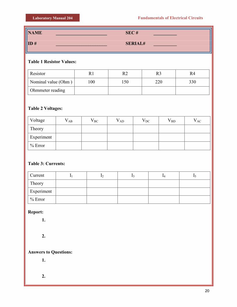
Table 1 Resistor Values: Resistor R1 R2 R3 R4
Nominal value (Ohm ) 100 150 220 330
Ohmmeter reading
Table 2 Voltages:
Voltage VAB VBC VAD VDC VBD VAC
Theory
Experiment
% Error
Table 3: Currents:
Current I1 I2 I3 I4 I5
Theory
Experiment
% Error
Report:
1.
2.
Answers to Questions:
1.
2.
Laboratory Manual 204 Fundamentals of Electrical Circuits
Experiment No. 4
Current and Voltage Divider Rules
Objective:
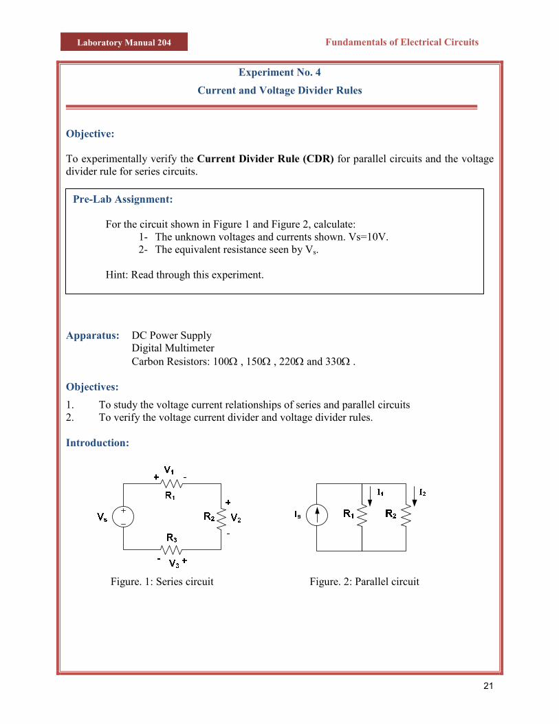
To experimentally verify the Current Divider Rule (CDR) for parallel circuits and the voltage divider rule for series circuits.
Apparatus: DC Power Sup Digital Multim Carbon Resisto Objectives:
1. To study the voltage cu2. To verify the voltage c Introduction:
Figure. 1: Series cir
Pre-Lab Assignment: For the circuit shown
1- The unkn2- The equiv
Hint: Read through th
in Figure 1 and Figure 2, calculate: own voltages and currents shown. Vs=10V. alent resistance seen by Vs.
is experiment.
21
ply eter rs: 100Ω , 150Ω , 220Ω and 330Ω .
rrent relationships of series and parallel circuits urrent divider and voltage divider rules.
cuit
Figure. 2: Parallel circuit
Laboratory Manual 204 Fundamentals of Electrical Circuits
22
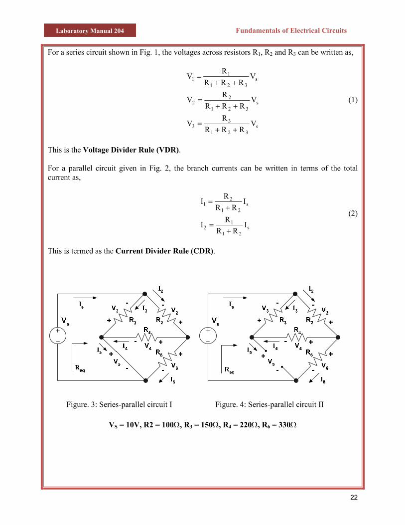
For a series circuit shown in Fig. 1, the voltages across resistors R1, R2 and R3 can be written as,
s321
33
s321
22
s321
11
VRRR
RV
VRRR
RV
VRRR
RV
++=
++=
++=
(1)
This is the Voltage Divider Rule (VDR). For a parallel circuit given in Fig. 2, the branch currents can be written in terms of the total current as,
s21
12
s21
21
IRR
RI
IRR
RI
+=
+=
(2)
This is termed as the Current Divider Rule (CDR).
Figure. 3: Series-parallel circuit I
Figure. 4: Series-parallel circuit II
VS = 10V, R2 = 100Ω, R3 = 150Ω, R4 = 220Ω, R6 = 330Ω
Laboratory Manual 204 Fundamentals of Electrical Circuits
23
Procedure:
Simulation
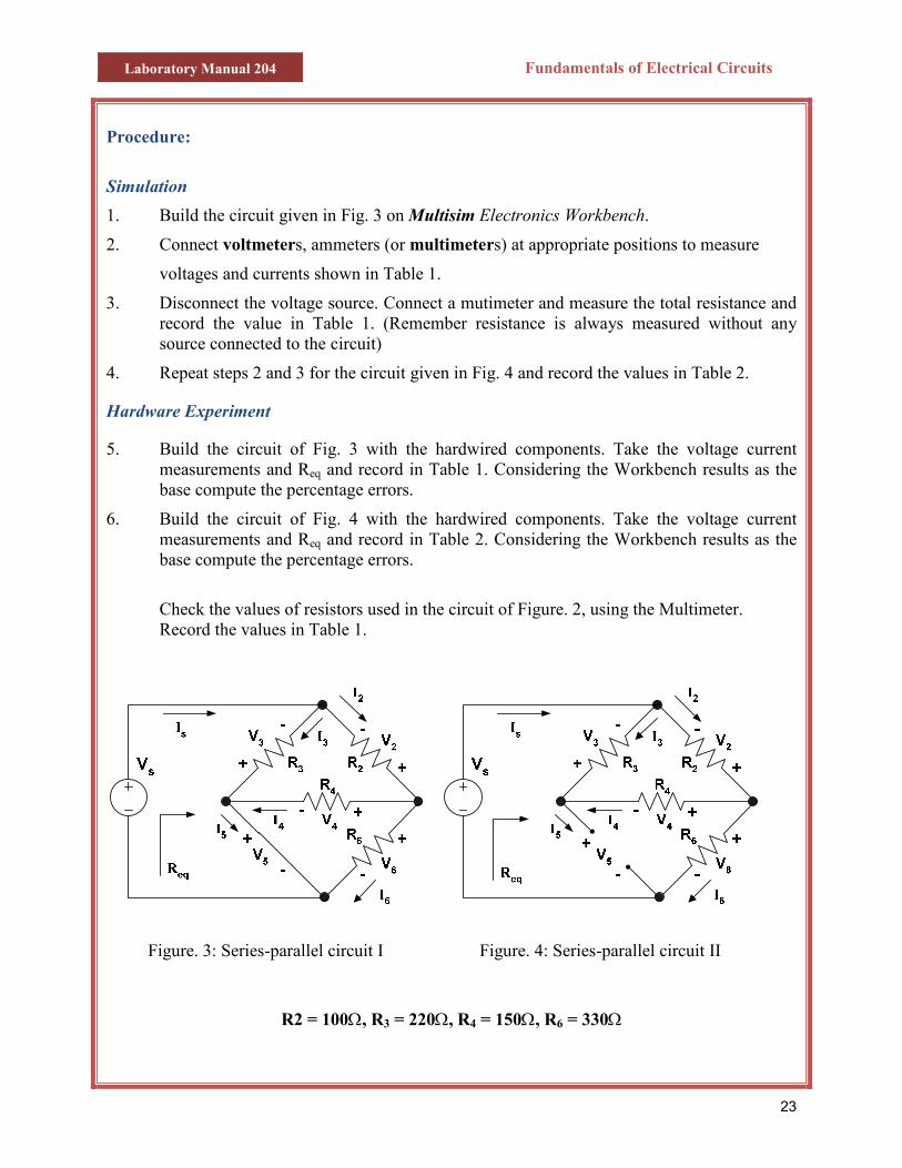
1. Build the circuit given in Fig. 3 on Multisim Electronics Workbench.
2. Connect voltmeters, ammeters (or multimeters) at appropriate positions to measure
voltages and currents shown in Table 1.
3. Disconnect the voltage source. Connect a mutimeter and measure the total resistance and record the value in Table 1. (Remember resistance is always measured without any source connected to the circuit)
4. Repeat steps 2 and 3 for the circuit given in Fig. 4 and record the values in Table 2.
Hardware Experiment
5. Build the circuit of Fig. 3 with the hardwired components. Take the voltage current measurements and Req and record in Table 1. Considering the Workbench results as the base compute the percentage errors.
6. Build the circuit of Fig. 4 with the hardwired components. Take the voltage current measurements and Req and record in Table 2. Considering the Workbench results as the base compute the percentage errors.
Check the values of resistors used in the circuit of Figure. 2, using the Multimeter. Record the values in Table 1.
Figure. 3: Series-parallel circuit I
Figure. 4: Series-parallel circuit II
R2 = 100Ω, R3 = 220Ω, R4 = 150Ω, R6 = 330Ω
Laboratory Manual 204 Fundamentals of Electrical Circuits
24
7. Connect the circuit of Figure. 2a and adjust the supply voltage Vs to 10 V, using the DC voltmeter.
8. Measure the entire unknown voltages and currents shown. Record their values in Table 2.
9. Measure Req using an Ohmmeter and record its values in Table 2. 10. Connect the circuit of Figure. 2b and adjust the supply voltage Vs to 10 V, using the DC
voltmeter. 11. Measure the entire unknown voltages and currents shown. Record their values in Table3
(recall that when measuring current by an ammeter, the ammeter should be placed in series with the element in which the current passes. Keep this fact in mind when measuring I5.
12. Measure Req. and record its value in Table 3.
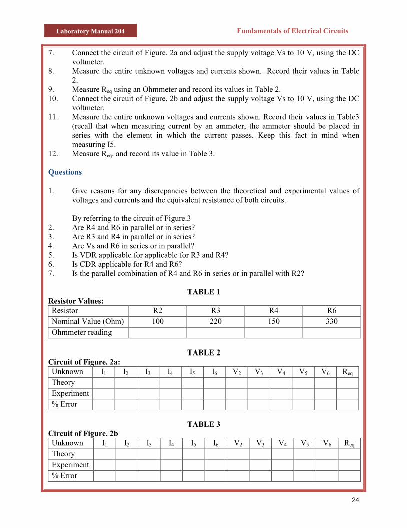
Questions 1. Give reasons for any discrepancies between the theoretical and experimental values of
voltages and currents and the equivalent resistance of both circuits. By referring to the circuit of Figure.3
2. Are R4 and R6 in parallel or in series? 3. Are R3 and R4 in parallel or in series? 4. Are Vs and R6 in series or in parallel? 5. Is VDR applicable for applicable for R3 and R4? 6. Is CDR applicable for R4 and R6? 7. Is the parallel combination of R4 and R6 in series or in parallel with R2?
TABLE 1
Resistor Values: Resistor R2 R3 R4 R6 Nominal Value (Ohm) 100 220 150 330 Ohmmeter reading
TABLE 2
Circuit of Figure. 2a: Unknown I1 I2 I3 I4 I5 I6 V2 V3 V4 V5 V6 Req
Theory Experiment % Error
TABLE 3
Circuit of Figure. 2b Unknown I1 I2 I3 I4 I5 I6 V2 V3 V4 V5 V6 Req
Theory Experiment % Error
Laboratory Manual 204 Fundamentals of Electrical Circuits
25
NAME ______________________ SEC # __________ ID # ______________________ SERIAL# __________
Answers to Questions:
1.
2.
3.
4.
5.
6.
7.
Laboratory Manual 204
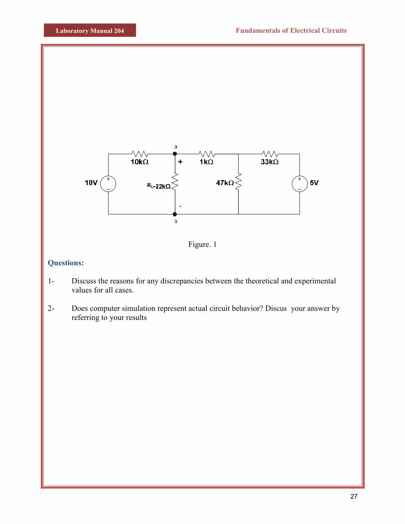
Objective: The objective of this experiment is to verify superposition theorem experimentally and using simulation. Pre- Lab Assignment: For the circuit shown Figure 1:
1. Find the & superposition.2. Record your values in Table 2 and 3
Note:
• , are due to 5 V Source • , are due to 10 V Source• & are due to both sources
Apparatus: DC Power Supply (Two) Digital Multimeter. Carbon Resistors: 10 k PC for simulation with Introduction The voltage and current responses in a network from two or more sources acting simultaneously can be obtained as the sum of the responses from each source acting alone with other sources deactivated. A deactivated current source is an open circuit. A deactivated voltashort circuit. Procedure: Note: do all the steps using computer simulation and experimentally. Step 1 is experimental only. 1. Check the values of the resistors using the multimeter. Record the values in Table.1.2. Connect the circuit of Figure.1 and measure 3. Deactivate the 10 V source and measure 4. Reactivate the 10 V sources and deactivate the 5 V source. Measure 5. Record the results in Tables 2 and 3
Fundamentals of Electrical Circuits
Experiment No. 5
Superposition Theorem
this experiment is to verify superposition theorem experimentally and using
superposition. Record your values in Table 2 and 3
are due to 5 V Source are due to 10 V Source are due to both sources
DC Power Supply (Two) Digital Multimeter.
Carbon Resistors: 10 kΩ, 22 kΩ, 33 kΩ, 47 kΩ, and 1 kΩ.PC for simulation with multisim
and current responses in a network from two or more sources acting simultaneously can be obtained as the sum of the responses from each source acting alone with other sources deactivated. A deactivated current source is an open circuit. A deactivated volta
Note: do all the steps using computer simulation and experimentally.
Check the values of the resistors using the multimeter. Record the values in Table.1.Connect the circuit of Figure.1 and measure & Deactivate the 10 V source and measure &
the 10 V sources and deactivate the 5 V source. Measure , and Record the results in Tables 2 and 3
Fundamentals of Electrical Circuits
26
this experiment is to verify superposition theorem experimentally and using
.
and current responses in a network from two or more sources acting simultaneously can be obtained as the sum of the responses from each source acting alone with other sources deactivated. A deactivated current source is an open circuit. A deactivated voltage source is a
Check the values of the resistors using the multimeter. Record the values in Table.1.
, and
Laboratory Manual 204 Fundamentals of Electrical Circuits
27
Figure. 1
Questions: 1- Discuss the reasons for any discrepancies between the theoretical and experimental
values for all cases. 2- Does computer simulation represent actual circuit behavior? Discus your answer by
referring to your results
Laboratory Manual 204
NAME ____________________ ID # ____________________
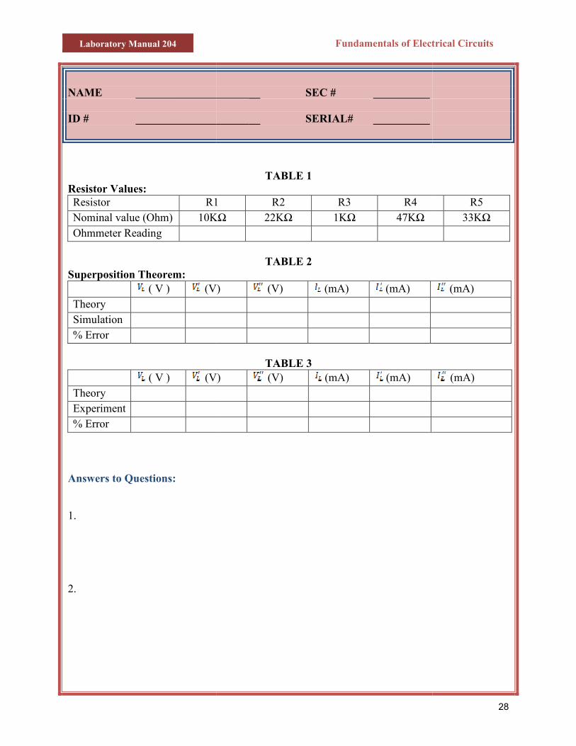
Resistor Values: Resistor R1Nominal value (Ohm) 10KOhmmeter Reading
Superposition Theorem: ( V ) (V)Theory Simulation % Error
( V ) (V)Theory Experiment % Error
Answers to Questions:
1.
2.
Fundamentals of Electrical Circuits
______________________ SEC # __________
______________________ SERIAL# __________
TABLE 1
R1 R2 R3 R4 10KΩ 22KΩ 1KΩ 47KΩ
TABLE 2
(V) (V) (mA) (mA)
TABLE 3 (V) (V) (mA) (mA)
Fundamentals of Electrical Circuits
28
R5 33KΩ
(mA)
(mA)
Laboratory Manual 204 Fundamentals of Electrical Circuits
Experiment No. 6
THEVENIN / NORTON Theorems and Maximum Power Transfer Objective: 1- To experimentally verify the Thevenin and Norton Theorems. 2- To experimentally verify the Maximum Power Transfer Theorem for resistive circuits. Apparatus: Theory:
• Theven A two–tecircuit vequivale •••• Norto
A two teshort cirequivalenis equal to
Pre- Lab Ass For th
1- F2- U
wRc
3- C4- F
M
ignment:
e circuit shown Figure 1: ind the VTH, ISC and Rth seen by RL. se the Thevenin’s equivalent circuit you obtained to find the values of VL hen L is varied from 2.5 K to 10.5 K in steps of 1 K Ohms. Calculate VL in each ase. alculate the power PL absorbed by RL in each case of step 2. ind the value of RL for Maximum Power Transfer and the value of the aximum Power.
29
DC Power Supply (Two) Digital Multimeter. Carbon Resistors: 10 kΩ, 22 kΩ, 33 kΩ, 47 kΩ, and 1 kΩ. Decade Resistor Box.
in’s Theorem:
rminal network can be replaced by a voltage source with the value equal the open oltage across its terminals, in series with a resistor with the value equal to the nt resistance of the network.
n’s Theorem: rminal network can be replaced by a current source with the value equal to the cuit current at its terminal, in parallel with a resistor with the value equal to the t resistance of the network. The equivalent resistance of a two–terminal network the open circuit voltage divided by the short circuit current.
Laboratory Manual 204 Fundamentals of Electrical Circuits
30
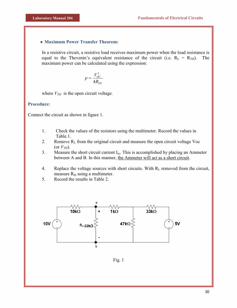
•••• Maximum Power Transfer Theorem:
In a resistive circuit, a resistive load receives maximum power when the load resistance is equal to the Thevenin’s equivalent resistance of the circuit (i.e. RL = RTH). The maximum power can be calculated using the expression:
TH
OC
RV
p4
2
=
where VTH is the open circuit voltage. Procedure: Connect the circuit as shown in figure 1.
1. Check the values of the resistors using the multimeter. Record the values in Table.1.
2. Remove RL from the original circuit and measure the open circuit voltage Voc (or VTH).
3. Measure the short circuit current Isc. This is accomplished by placing an Ammeter between A and B. In this manner, the Ammeter will act as a short circuit.
4. Replace the voltage sources with short circuits. With RL removed from the circuit,
measure Rth using a multimeter. 5. Record the results in Table 2.
Fig. 1

Laboratory Manual 204 Fundamentals of Electrical Circuits
31
Maximum Power Transfer:
6. Reconnect the circuit as shown in Figure 1, but replace the 22 KΩ resistor
between A and B and by a variable resistor (i.e. RL in this case is the variable resistor).
7. Vary RL from 2.5 KΩ to 10.5 KΩ in steps of 1 KΩ and measure VL in each case. 8. Record the results in Table 3. 9. Calculate PL from Step. 7 above and record the results in Table 4.
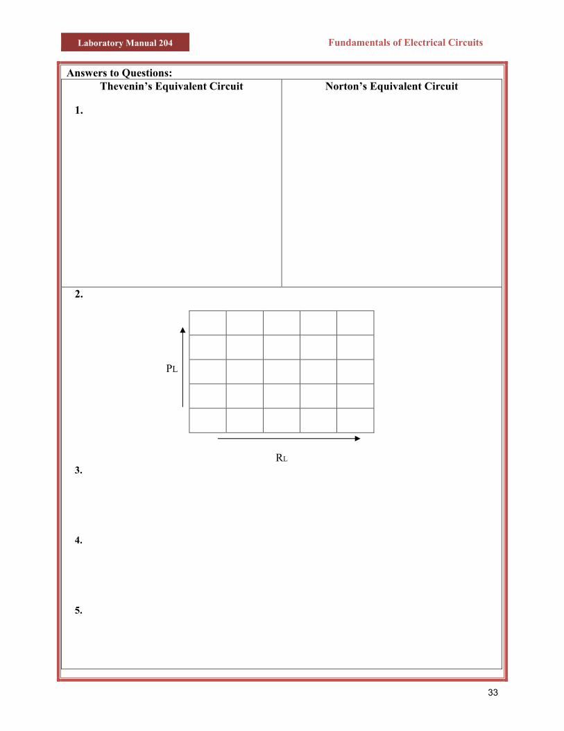
Questions:
1. Draw the Thevenin’s and Norton’s equivalent circuit obtained experimentally. 2. Plot the theoretical and experimental values of PL versus RL (on the same graph)
and compare the two graphs. 3. Discuss the reasons for any discrepancies between the theoretical and
experimental values for all cases. 4. Thevenin’s and Norton’s Theorem are very useful. List at least two reasons for it 5. Is the Maximum Power Theorem verified experimentally? Explain.
Laboratory Manual 204 Fundamentals of Electrical Circuits
32
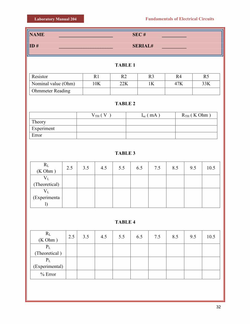
NAME ______________________ SEC # __________ ID # ______________________ SERIAL# __________
TABLE 1
Resistor R1 R2 R3 R4 R5 Nominal value (Ohm) 10K 22K 1K 47K 33K Ohmmeter Reading
TABLE 2
VTH ( V ) Isc ( mA ) RTH ( K Ohm ) Theory Experiment Error
TABLE 3
RL (K Ohm )
2.5 3.5 4.5 5.5 6.5 7.5 8.5 9.5 10.5
VL (Theoretical)
VL
(Experimental)
TABLE 4
RL (K Ohm )
2.5 3.5 4.5 5.5 6.5 7.5 8.5 9.5 10.5
PL
(Theoretical )
PL (Experimental)
% Error
Laboratory Manual 204 Fundamentals of Electrical Circuits
33
Answers to Questions: Thevenin’s Equivalent Circuit
1.
Norton’s Equivalent Circuit
2.
PL
RL
3. 4. 5.
Laboratory Manual 204 Fundamentals of Electrical Circuits
34
Experiment No. 7
The Oscilloscope and Function Generator
Introduction
The Oscilloscope is one of the most important electronic instruments available for making circuit measurements. It displays a curve plot of time-varying voltage on the Oscilloscope screen. The controls on the Oscilloscope are as follows:
1. The TIME/DIV control adjusts the time scale on the horizontal axis in time per division. The X_POS control determines the horizontal position where the curve plot begins.
2. The CHANNEL A control adjusts the volts per division on the vertical axis for the channel A curve plot. The POSITION control located in top of CHANNEL A determines the vertical position of the channel A curve plot relative to the horizontal axis. Selecting AC places a capacitance between the channel A vertical input and the circuit testing point. Selecting “GORUND” connects channel A vertical input to ground.
3. Same thing applies to CHANNEL B.
The Function Generator The Function Generator is a voltage source that supplies different time-varying voltage functions. The Function Generator can supply Sine Wave, Square Wave, and Triangular Wave voltage functions. The waveshape, frequency, amplitude, and DC offset can be easily changed. The controls on the Function Generator are as follows:
1. You can select a waveshape by selecting the appropriate waveshape (Sine wave, Square Wave and Triangular Wave) on the top of the Function Generator.
2. The frequency control allows you adjust the frequency of the output voltage. Select the frequency button and select the frequency with the appropriate scale.
3. The AMPLITUDE buttons allows you to adjust the peak to peak value or RMS of the output voltage. The peak to peak value is twice the amplitude setting.
4. The OFFSET buttons adjusts the DC level of the voltage curve generated by the Function Generator. When selecting the DC option on the Oscilloscope, an offset of 0 positions the curve plot along the x-axis with an equal positive and negative voltage setting. A positive offset raises the curve plot above the x-axis and a negative offset lowers the curve plot below the x-axis.

Laboratory Manual 204 Fundamentals of Electrical Circuits
35
Procedure 1. Connect the output of the Function Generator to CHANNEL A on the Oscilloscope. 2. Turn the Function Generator and select the Sine Wave button. Set frequency to 1 kHz and 2
Vp-p. Set the DC offset to 0 V DC. 3. Turn on the Oscilloscope and select the GROUND button. Using the POSITON control on
the top, bring your line to the center of the screen. Now select the AC position.
4. Select the TIME/DIV to 0.2ms and CHANNEL A to 0.5 V/DIV.
Question: What was the time period (T) and the frequency of your signal? 5. Select the “GROUND” on the Oscilloscope channel A. Question: What change occurred on the Oscilloscope Channel A curve plot? Explain. 6. Change the Oscilloscope channel A to 1V/div. Question: What change occurred on the Oscilloscope Channel A curve plot? Explain. 7. Change the Oscilloscope Time Base to 0.1ms/div. Question: What change occurred on the Oscilloscope Channel A curve plot? What is the period and the frequency of your signal? Compare the results to that of step 4. 8. Return the Oscilloscope time base to 0.2m/DIV and CHANNEL A to 0.5V/DIV. Select the
Triangular Wave shape on the Function Generator. Question: What change occurred on the Oscilloscope curve plot? 9. Select the Square Wave on the Function Generator and run the analysis again. Question: What change occurred on the Oscilloscope curve plot? 10. Change the AMPLITUDE on the Function Generator to 2Vp-p Question: What change occurred on the Oscilloscope curve plot? Explain. 11. Change the frequency on the Function Generator to 2 kHz. Question: What change occurred on the Oscilloscope curve plot? Explain. 12. Change the offset on the Function Generator to 1V. Question: What change occurred on the Oscilloscope curve plot? Explain. 13. Select the DC setting on CHANNEL A of the oscilloscope. Question: What change occurred on the Oscilloscope curve plot? Explain.

Laboratory Manual 204 Fundamentals of Electrical Circuits
36
NAME ______________________ SEC # __________ ID # ______________________ SERIAL# __________
Answers to Questions in Procedures Question of Step 4 Question of Step 5 Question of Step 6 Question of Step 7 Question of Step 8
Laboratory Manual 204 Fundamentals of Electrical Circuits
37
Question of Step 9 Question of Step 10 Question of Step 11 Question of Step 12 Question of Step 13 Question of Step 13
Laboratory Manual 204 Fundamentals of Electrical Circuits
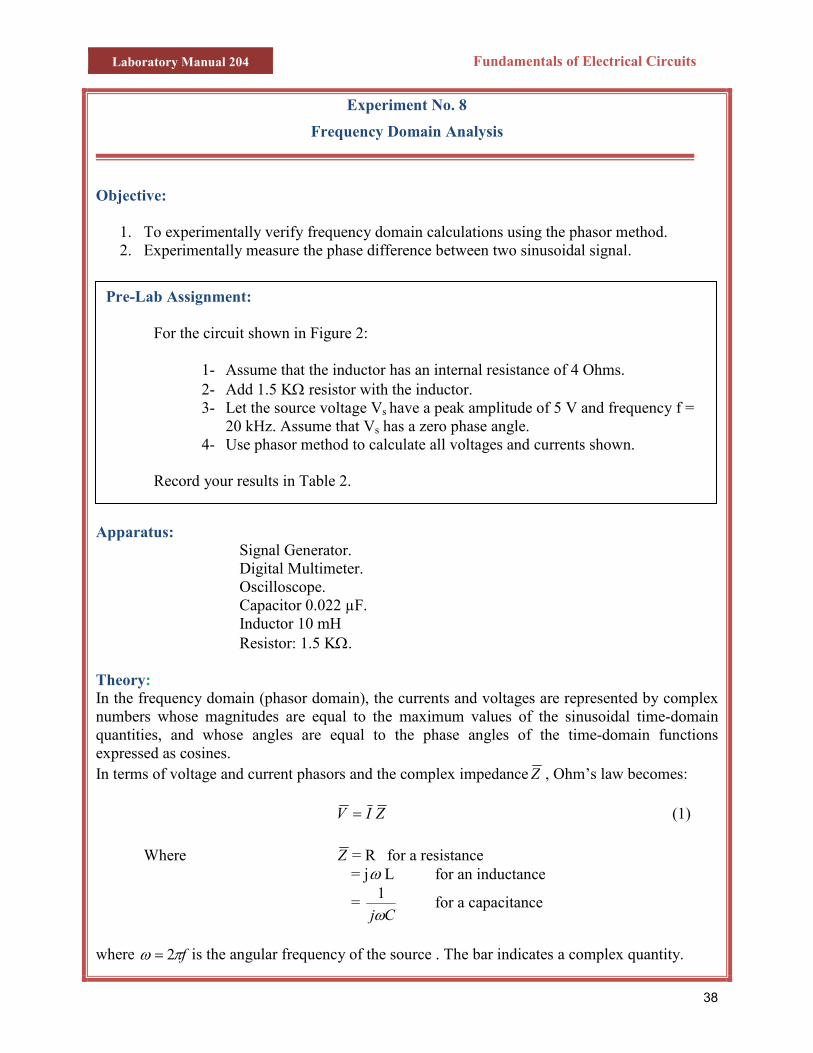
Experiment No. 8
Frequency Domain Analysis
Objective:
1. To experimentally verify frequency domain calculations using the phasor method. 2. Experimentally measure the phase difference between two sinusoidal signal.
Apparatus:
Theory: In the frequency domanumbers whose magnquantities, and whoseexpressed as cosines. In terms of voltage and
Where
where fπω 2= is the an
Pre-Lab Assignmen For the circui
1- As2- Ad3- Le
204- Us
Record your r
t:
t shown in Figure 2:
sume that the inductor has an internal resistance of 4 Ohms. d 1.5 KΩ resistor with the inductor. t the source voltage Vs have a peak amplitude of 5 V and frequency f = kHz. Assume that Vs has a zero phase angle. e phasor method to calculate all voltages and currents shown.
esults in Table 2.
38
Signal Generator. Digital Multimeter. Oscilloscope. Capacitor 0.022 µF. Inductor 10 mH Resistor: 1.5 KΩ.
in (phasor domain), the currents and voltages are represented by complex itudes are equal to the maximum values of the sinusoidal time-domain angles are equal to the phase angles of the time-domain functions
current phasors and the complex impedance Z , Ohm’s law becomes:
ZIV = (1)
Z = R for a resistance = jω L for an inductance
= Cjω
1 for a capacitance
gular frequency of the source . The bar indicates a complex quantity.
Laboratory Manual 204 Fundamentals of Electrical Circuits
39
In general, for =V 1θ∠V and 2θ∠= II , the impedance 21 θθ −∠=IV
Z
Analytically, frequency-domain circuits are treated by the same method as used in DC circuits, except that the algebra of complex numbers is used.
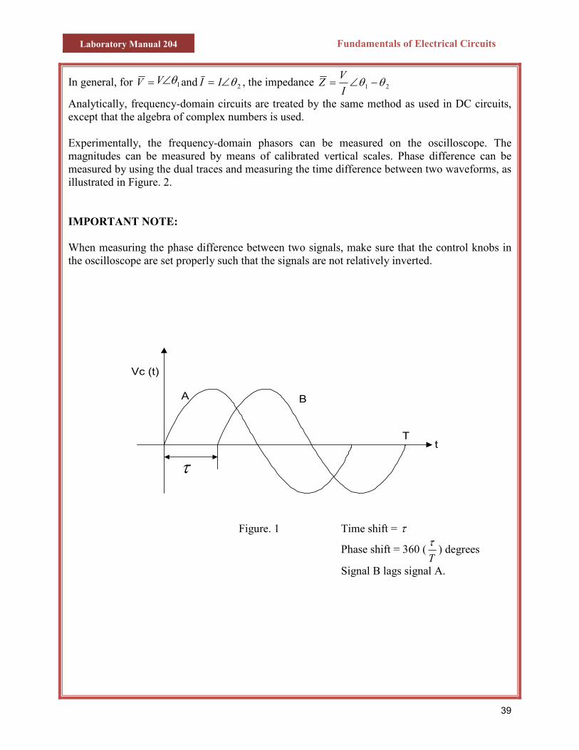
Experimentally, the frequency-domain phasors can be measured on the oscilloscope. The magnitudes can be measured by means of calibrated vertical scales. Phase difference can be measured by using the dual traces and measuring the time difference between two waveforms, as illustrated in Figure. 2.
IMPORTANT NOTE: When measuring the phase difference between two signals, make sure that the control knobs in the oscilloscope are set properly such that the signals are not relatively inverted.
Figure. 1 Time shift = τ
Phase shift = 360 (Tτ
) degrees
Signal B lags signal A.
Vc (t)
τ
A B
Tt
Laboratory Manual 204 Fundamentals of Electrical Circuits
40
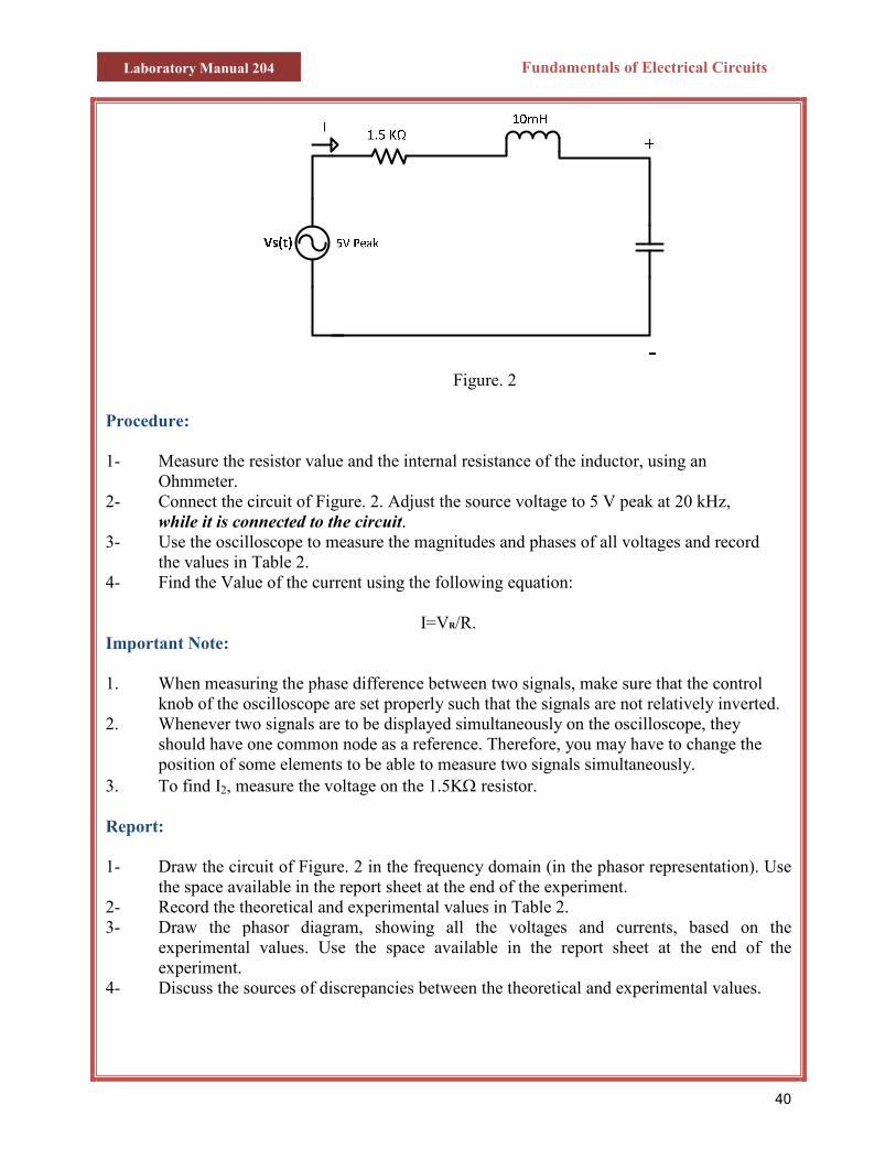
Figure. 2
Procedure:
1- Measure the resistor value and the internal resistance of the inductor, using an
Ohmmeter. 2- Connect the circuit of Figure. 2. Adjust the source voltage to 5 V peak at 20 kHz,
while it is connected to the circuit. 3- Use the oscilloscope to measure the magnitudes and phases of all voltages and record
the values in Table 2. 4- Find the Value of the current using the following equation:
I=VR/R. Important Note: 1. When measuring the phase difference between two signals, make sure that the control
knob of the oscilloscope are set properly such that the signals are not relatively inverted. 2. Whenever two signals are to be displayed simultaneously on the oscilloscope, they
should have one common node as a reference. Therefore, you may have to change the position of some elements to be able to measure two signals simultaneously.
3. To find I2, measure the voltage on the 1.5KΩ resistor. Report: 1- Draw the circuit of Figure. 2 in the frequency domain (in the phasor representation). Use
the space available in the report sheet at the end of the experiment. 2- Record the theoretical and experimental values in Table 2. 3- Draw the phasor diagram, showing all the voltages and currents, based on the
experimental values. Use the space available in the report sheet at the end of the experiment.
4- Discuss the sources of discrepancies between the theoretical and experimental values.
Laboratory Manual 204 Fundamentals of Electrical Circuits
41
Questions: 1. For a resistance and capacitance in series with a voltage source, show that it is possible to
draw a phasor diagram for the current and all voltages from magnitude measurement of these quantities only. Illustrate your answer graphically.
2. The equivalent impedance of a capacitor in series with an inductor is equivalent to a
short circuit (i.e. equal to zero) at a certain frequency. Derive an expression for this frequency.
3. The equivalent impedance of a capacitor in parallel with an inductor is equivalent to an
open circuit (i.e. equal to infinity) at a certain frequency. Derive an expression for this frequency.
Laboratory Manual 204 Fundamentals of Electrical Circuits
42
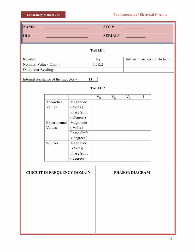
NAME ______________________ SEC # __________ ID # ______________________ SERIAL# __________
TABLE 1
Resistor R1 Internal resistance of Inductor Nominal Value ( Ohm ) 1.5KΩ Ohmmeter Reading
Internal resistance of the inductor = Ω
TABLE 2
VR VL VC I
Theoretical Values
Magnitude ( Volts )
Phase Shift ( Degree )
Experimental Values
Magnitude ( Volts )
Phase Shift ( degrees )
% Error Magnitude (Volts)
Phase Shift ( degrees )
CIRCUIT IN FREQUENCY DOMAIN
PHASOR DIAGRAM
Laboratory Manual 204 Fundamentals of Electrical Circuits
43
Experiment No. 9
Maximum Power Transfer
Objective:
1. To obtain maximum output power from a sinusoidal source with an internal impedance
2. To experimentally verify the theory of maximum power transfer.
3.
Apparatus:
• Signal Generator • Digital Multimeter • Decade Resistance Boxes RDB and RDA • Decade Capacitance Box CDA • Inductor (10 mH) • Resistance (100 Ohms)
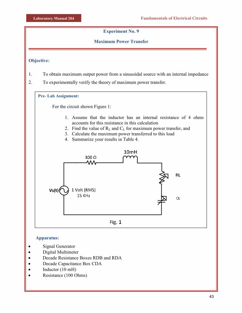
Pre- Lab Assignment: For the circuit shown Figure 1:
1. Assume that the inductor has an internal resistance of 4 ohms accounts for this resistance in this calculation
2. Find the value of RL and CL for maximum power transfer, and 3. Calculate the maximum power transferred to this load 4. Summarize your results in Table 4.
Laboratory Manual 204 Fundamentals of Electrical Circuits
44
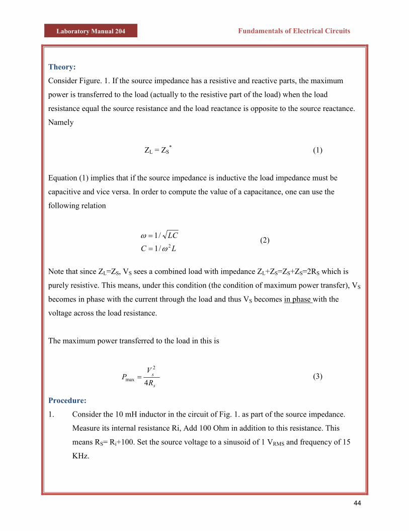
Theory:
Consider Figure. 1. If the source impedance has a resistive and reactive parts, the maximum
power is transferred to the load (actually to the resistive part of the load) when the load
resistance equal the source resistance and the load reactance is opposite to the source reactance.
Namely
ZL = ZS* (1)
Equation (1) implies that if the source impedance is inductive the load impedance must be
capacitive and vice versa. In order to compute the value of a capacitance, one can use the
following relation
LC
LC2/1
/1
ω
ω
=
= (2)
Note that since ZL=ZS, VS sees a combined load with impedance ZL+ZS=ZS+ZS=2RS which is
purely resistive. This means, under this condition (the condition of maximum power transfer), VS
becomes in phase with the current through the load and thus VS becomes in phase with the
voltage across the load resistance.
The maximum power transferred to the load in this is
s
s
R
VP
4
2
max = (3)
Procedure:
1. Consider the 10 mH inductor in the circuit of Fig. 1. as part of the source impedance.
Measure its internal resistance Ri, Add 100 Ohm in addition to this resistance. This
means RS= Ri+100. Set the source voltage to a sinusoid of 1 VRMS and frequency of 15
KHz.
Laboratory Manual 204 Fundamentals of Electrical Circuits
45
2. With RL set the value of RS, vary C from 0.007 µF to 0.015 µF in steps of 0.001 µF (use
two decade capacitors in parallel). Measure the voltage across RL in each case,
maintaining an input voltage of 1 VRMS. Record the values in table 2.
3. Display the source voltage and the voltage across RL simultaneously on the oscilloscope.
Vary C and notice the phase shift between the two signals. Record the value of C that
makes the two signals in phase.
4. With C set at the value found in step 3, vary RL from 80-120 and measure the voltage
across RL in each case, again maintaining an input voltage of 1 V RMS. Record the values
in table 4.
Note: Record your results in Table No. 1, 2, 3 & 4 and answer the questions.
Questions:
1) What is the phase difference between the current and the voltage source when maximum
power transfer is achieved?
2) If the frequency of the source is doubled, what change should be done to maintain
maximum power transfer to the load? How does this change affect the value of the
maximum power? Explain.
3) Comment on the causes of errors between the measure and calculated values.
Laboratory Manual 204 Fundamentals of Electrical Circuits
46
NAME ______________________ SEC # __________ ID # ______________________ SERIAL# __________
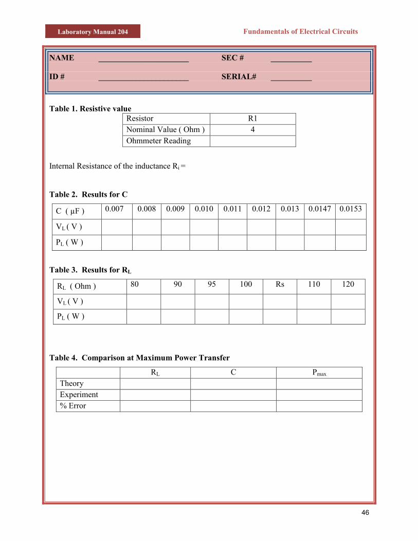
Table 1. Resistive value
Resistor R1 Nominal Value ( Ohm ) 4 Ohmmeter Reading
Internal Resistance of the inductance Ri =
Table 2. Results for C
C ( µF ) 0.007 0.008 0.009 0.010 0.011 0.012 0.013 0.0147 0.0153
VL ( V )
PL ( W )
Table 3. Results for RL
RL ( Ohm ) 80 90 95 100 Rs 110 120
VL ( V )
PL ( W )
Table 4. Comparison at Maximum Power Transfer
RL C Pmax Theory Experiment % Error
Laboratory Manual 204 Fundamentals of Electrical Circuits
Experiment No. 10
Average and RMS Values
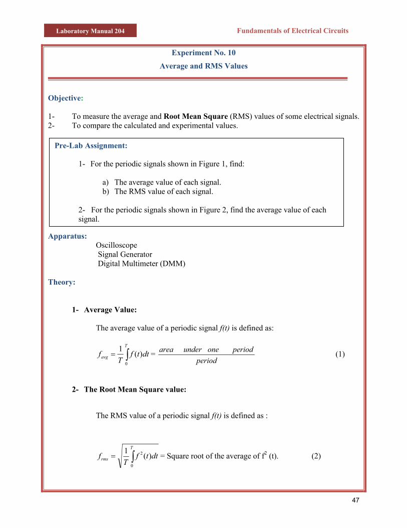
Objective:
1- To measure the average and Root Mean Square (RMS) values of some electrical signals. 2- To compare the calculated and experimental values.
Apparatus:
Oscilloscope Signal Gene Digital Mul Theory:
1- Average Value: The average
∫=T
avg fT
f0
(1
2- The Root Mean
The RMS va
∫=T
rms Tf
0
1
Pre-Lab Assignment:
1- For the period
a) The avb) The RM
2- For the periodsignal.
ic signals shown in Figure 1, find:
erage value of each signal. S value of each signal.
ic signals shown in Figure 2, find the average value of each
47
rator timeter (DMM)
value of a periodic signal f(t) is defined as:
dtt) = period
periodoneunderarea (1)
Square value:
lue of a periodic signal f(t) is defined as :
dttf 2 )( = Square root of the average of f2 (t). (2)
Laboratory Manual 204 Fundamentals of Electrical Circuits
48
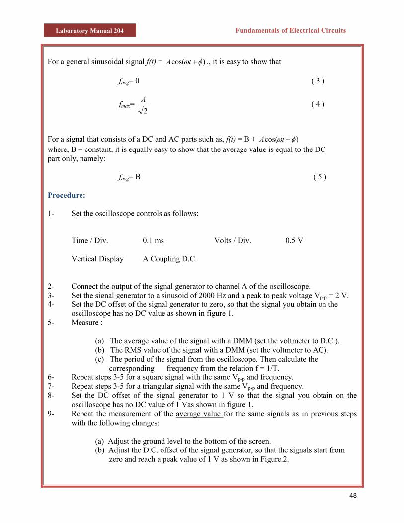
For a general sinusoidal signal f(t) = )cos( φω +tA ., it is easy to show that
favg= 0 ( 3 )
fmax= 2
A ( 4 )
For a signal that consists of a DC and AC parts such as, f(t) = B + )cos( φω +tA where, B = constant, it is equally easy to show that the average value is equal to the DC part only, namely:
favg= B ( 5 )
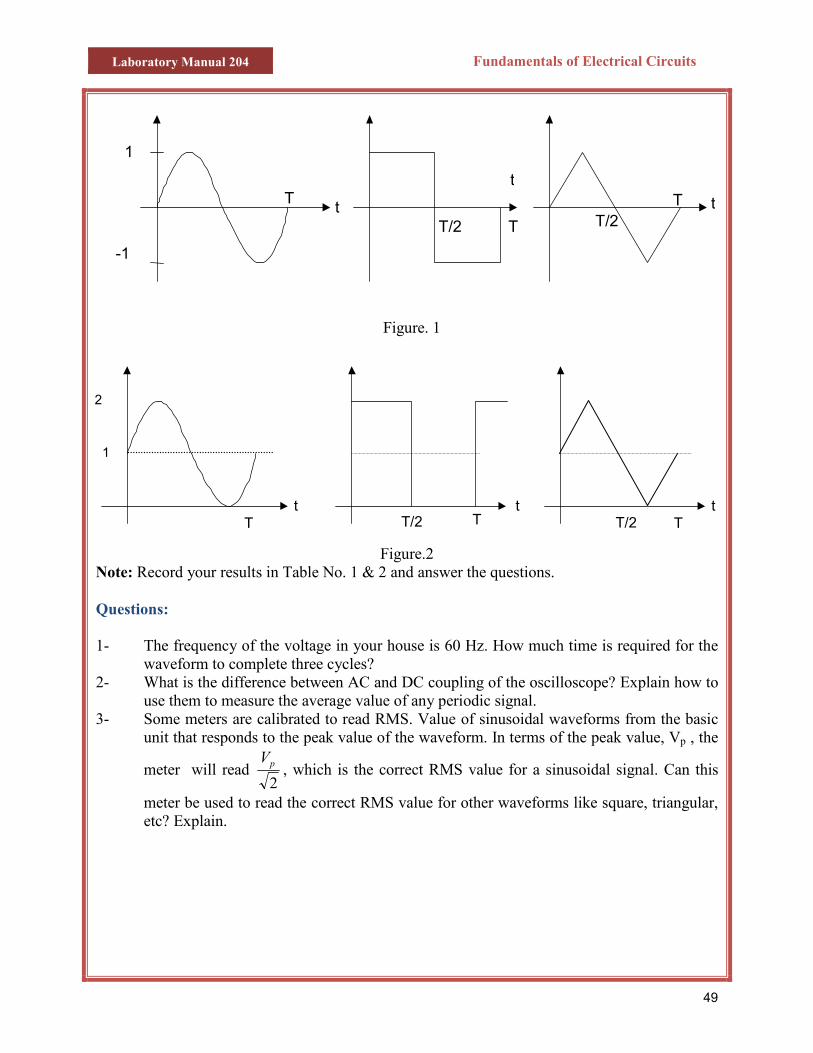
Procedure: 1- Set the oscilloscope controls as follows: Time / Div. 0.1 ms Volts / Div. 0.5 V Vertical Display A Coupling D.C. 2- Connect the output of the signal generator to channel A of the oscilloscope. 3- Set the signal generator to a sinusoid of 2000 Hz and a peak to peak voltage Vp-p = 2 V. 4- Set the DC offset of the signal generator to zero, so that the signal you obtain on the
oscilloscope has no DC value as shown in figure 1. 5- Measure :
(a) The average value of the signal with a DMM (set the voltmeter to D.C.). (b) The RMS value of the signal with a DMM (set the voltmeter to AC). (c) The period of the signal from the oscilloscope. Then calculate the corresponding frequency from the relation f = 1/T.
6- Repeat steps 3-5 for a square signal with the same Vp-p and frequency. 7- Repeat steps 3-5 for a triangular signal with the same Vp-p and frequency. 8- Set the DC offset of the signal generator to 1 V so that the signal you obtain on the
oscilloscope has no DC value of 1 Vas shown in figure 1. 9- Repeat the measurement of the average value for the same signals as in previous steps
with the following changes:
(a) Adjust the ground level to the bottom of the screen. (b) Adjust the D.C. offset of the signal generator, so that the signals start from zero and reach a peak value of 1 V as shown in Figure.2.
Laboratory Manual 204 Fundamentals of Electrical Circuits
49
Figure. 1
Figure.2 Note: Record your results in Table No. 1 & 2 and answer the questions. Questions: 1- The frequency of the voltage in your house is 60 Hz. How much time is required for the
waveform to complete three cycles? 2- What is the difference between AC and DC coupling of the oscilloscope? Explain how to
use them to measure the average value of any periodic signal. 3- Some meters are calibrated to read RMS. Value of sinusoidal waveforms from the basic
unit that responds to the peak value of the waveform. In terms of the peak value, Vp , the
meter will read 2pV
, which is the correct RMS value for a sinusoidal signal. Can this
meter be used to read the correct RMS value for other waveforms like square, triangular, etc? Explain.
1
-1
T tT/2
t
T/2 T t
T
T t
T/2
T/2 Tt
1
2
T t
Laboratory Manual 204 Fundamentals of Electrical Circuits
50
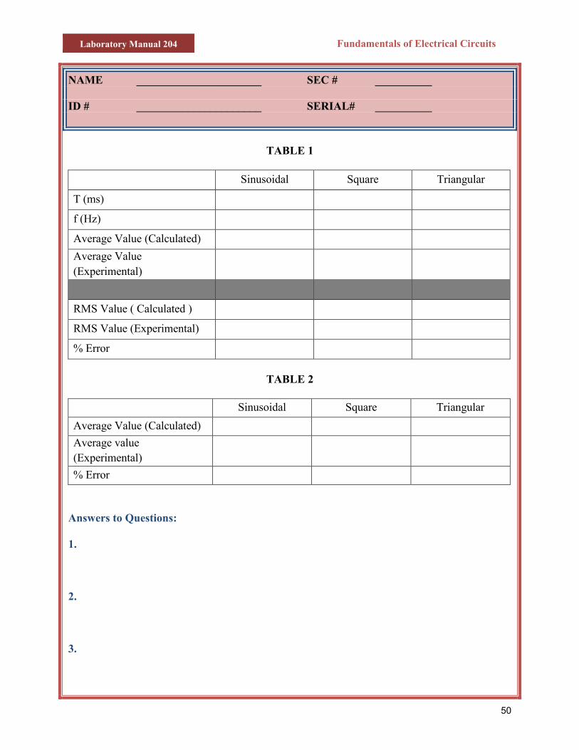
NAME ______________________ SEC # __________ ID # ______________________ SERIAL# __________
TABLE 1
Sinusoidal Square Triangular
T (ms)
f (Hz)
Average Value (Calculated)
Average Value (Experimental)
RMS Value ( Calculated )
RMS Value (Experimental)
% Error
TABLE 2
Sinusoidal Square Triangular
Average Value (Calculated) Average value (Experimental)
% Error Answers to Questions: 1. 2. 3.

Laboratory Manual 204 Fundamentals of Electrical Circuits
51
Appendix I
Laboratory Manual 204 Fundamentals of Electrical Circuits
52
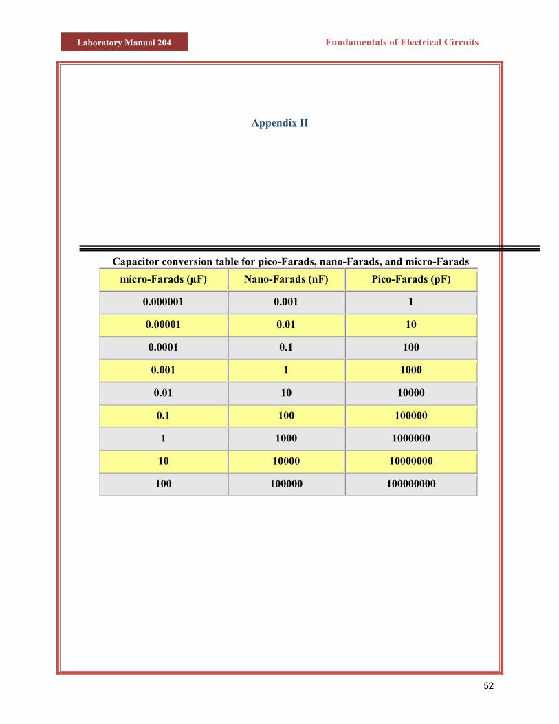
Appendix II
Capacitor conversion table for pico-Farads, nano-Farads, and micro-Farads
micro-Farads (µF) Nano-Farads (nF) Pico-Farads (pF)
0.000001 0.001 1
0.00001 0.01 10
0.0001 0.1 100
0.001 1 1000
0.01 10 10000
0.1 100 100000
1 1000 1000000
10 10000 10000000
100 100000 100000000
Laboratory Manual 204 Fundamentals of Electrical Circuits
53
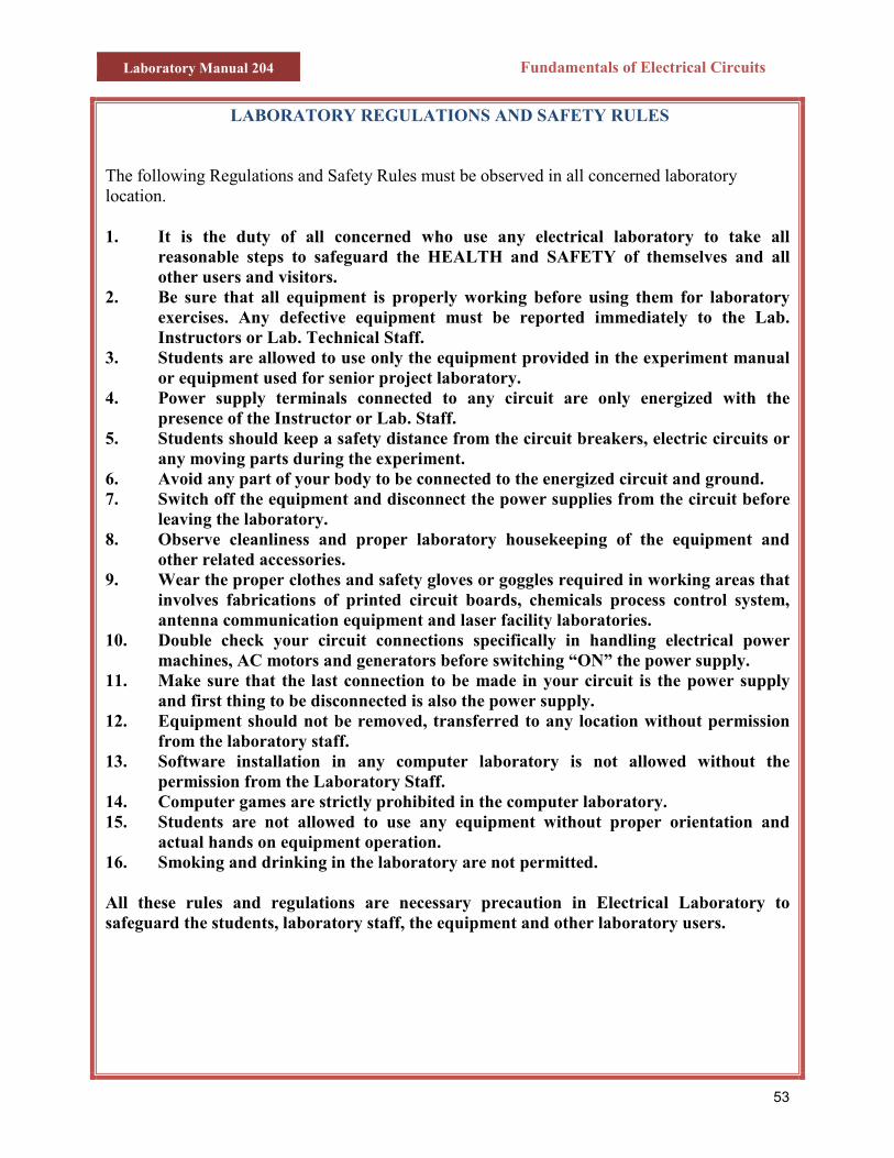
LABORATORY REGULATIONS AND SAFETY RULES
The following Regulations and Safety Rules must be observed in all concerned laboratory location. 1. It is the duty of all concerned who use any electrical laboratory to take all
reasonable steps to safeguard the HEALTH and SAFETY of themselves and all other users and visitors.
2. Be sure that all equipment is properly working before using them for laboratory exercises. Any defective equipment must be reported immediately to the Lab. Instructors or Lab. Technical Staff.
3. Students are allowed to use only the equipment provided in the experiment manual or equipment used for senior project laboratory.
4. Power supply terminals connected to any circuit are only energized with the presence of the Instructor or Lab. Staff.
5. Students should keep a safety distance from the circuit breakers, electric circuits or any moving parts during the experiment.
6. Avoid any part of your body to be connected to the energized circuit and ground. 7. Switch off the equipment and disconnect the power supplies from the circuit before
leaving the laboratory. 8. Observe cleanliness and proper laboratory housekeeping of the equipment and
other related accessories. 9. Wear the proper clothes and safety gloves or goggles required in working areas that
involves fabrications of printed circuit boards, chemicals process control system, antenna communication equipment and laser facility laboratories.
10. Double check your circuit connections specifically in handling electrical power machines, AC motors and generators before switching “ON” the power supply.
11. Make sure that the last connection to be made in your circuit is the power supply and first thing to be disconnected is also the power supply.
12. Equipment should not be removed, transferred to any location without permission from the laboratory staff.
13. Software installation in any computer laboratory is not allowed without the permission from the Laboratory Staff.
14. Computer games are strictly prohibited in the computer laboratory. 15. Students are not allowed to use any equipment without proper orientation and
actual hands on equipment operation. 16. Smoking and drinking in the laboratory are not permitted. All these rules and regulations are necessary precaution in Electrical Laboratory to safeguard the students, laboratory staff, the equipment and other laboratory users.