Fundamentals ofElectric Circuits

FiFt h Edition

Charles K. Alexander | Matthew n. o. Sadiku

Fundamentals of

Electric Circuits

FiFth Edition

Alexander

Sadiku

With its objective to present circuit analysis in a manner that is clearer, more interesting, and easier to understand than other texts, Fundamentals of Electric Circuits by Charles Alexander and Matthew Sadiku

has become the student choice for introductory electric circuits courses.

Building on the success of the previous editions, the fifth edition features the latest updates and advances in the field, while continuing to present material with an unmatched pedagogy and communication style.

Pedagogical Features

■ Problem-Solving Methodology. A six-step method for solving circuits problems is introduced in Chapter 1 and used consistently throughout the book to help students develop a systems approach to problem solving that leads to better understanding and fewer mistakes in mathematics and theory.

■ Matched Example Problems and Extended Examples. Each illustrative example is immediately followed by a practice problem and answer to test understanding of the preceding example. one extended example per chapter shows an example problem worked using a detailed outline of the six-step method so students can see how to practice this technique. Students follow the example step-by-step to solve the practice problem without having to flip pages or search the end of the book for answers.

■ Comprehensive Coverage of Material. not only is Fundamentals the most comprehensive text in terms of material, but it is also self-contained in regards to mathematics and theory, which means that when students have questions regarding the mathematics or theory they are using to solve problems, they can find answers to their questions in the text itself. they will not need to seek out other references.

■ Computer tools. PSpice® for Windows is used throughout the text with discussions and examples at the end of each appropriate chapter. MAtLAB® is also used in the book as a computational tool.

■ new to the fifth edition is the addition of 120 national instruments Multisim™ circuit files. Solutions for almost all of the problems solved using PSpice are also available to the instructor in Multisim.

■ We continue to make available KCidE for Circuits (a Knowledge Capturing integrated design Environment for Circuits).

■ An icon is used to identify homework problems that either should be solved or are more easily solved using PSpice, Multisim, and/or KCidE. Likewise, we use another icon to identify problems that should be solved or are more easily solved using MAtLAB.

Teaching Resources

McGraw-hill Connect® Engineering is a web-based assignment and assessment platform that gives students the means to better connect with their coursework, with their instructors, and with the important concepts that they will need to know for success now and in the future. Contact your McGraw-hill sales representative or visit www.connect.mcgraw-hill.com for more details.

the text also features a website of student and instructor resources. Check it out at www.mhhe.com/alexander.

MD

DA

LIM

1167970 10/30/11 CY

AN

MA

G Y

EL

O B

LA

CK

Fundamentals Of Electric Circuits 5th Edition Alexander Solutions ManualFull Download: https://testbanklive.com/download/fundamentals-of-electric-circuits-5th-edition-alexander-solutions-manual/

Full download all chapters instantly please go to Solutions Manual, Test Bank site: TestBankLive.com

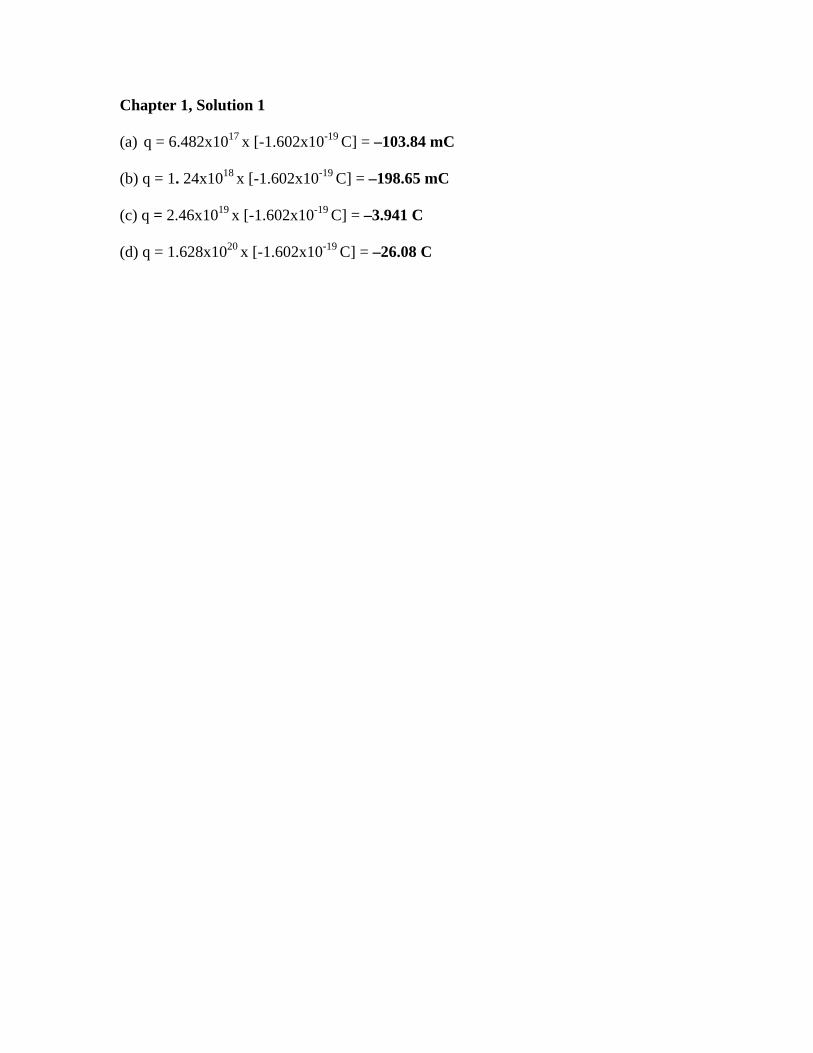
Chapter 1, Solution 1 (a) q = 6.482x1017

x [-1.602x10-19 C] = –103.84 mC

(b) q = 1. 24x1018

x [-1.602x10-19 C] = –198.65 mC

(c) q = 2.46x1019

x [-1.602x10-19 C] = –3.941 C

(d) q = 1.628x1020

x [-1.602x10-19 C] = –26.08 C

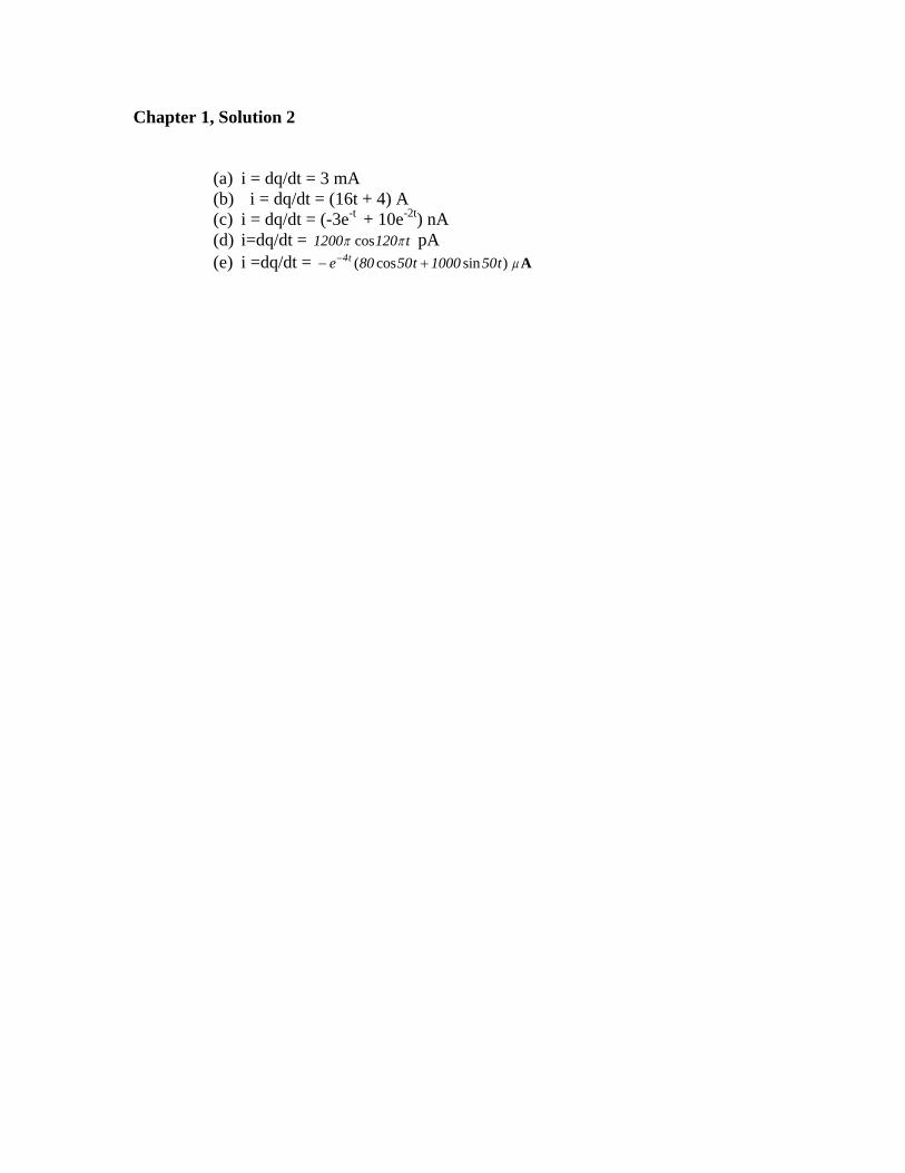
Chapter 1, Solution 2

(a) i = dq/dt = 3 mA (b) i = dq/dt = (16t + 4) A (c) i = dq/dt = (-3e-t + 10e-2t) nA (d) i=dq/dt = 1200 120 cos t pA (e) i =dq/dt = e t tt4 80 50 1000 50( cos sin ) A

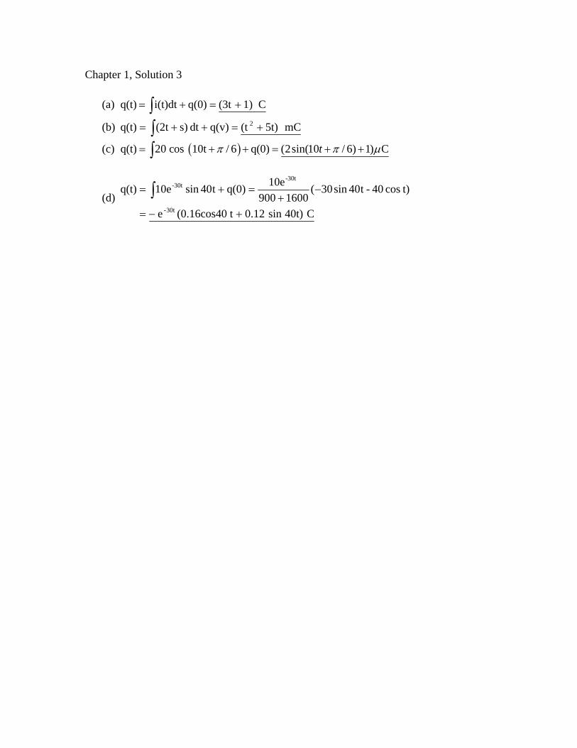
Chapter 1, Solution 3

(a) C 1)(3t q(0)i(t)dt q(t)

(b) mC 5t)(t 2 q(v)dt s)(2tq(t)

(c) q(t) 20 cos 10t / 6 q(0) (2sin(10 / 6) 1) Ct

(d)

C 40t) sin 0.12t(0.16cos40e 30t-

t)cos 40-t40sin30(1600900

e10q(0)t40sin10eq(t)

-30t30t-

Chapter 1, Solution 4 q = it = 7.4 x 20 = 148 C

Chapter 1, Solution 5

10 2

0

10125 C

02 4

tq idt tdt

Chapter 1, Solution 6

(a) At t = 1ms, 2

30

dt

dqi 15 A

(b) At t = 6ms, dt

dqi 0 A

(c) At t = 10ms,

4

30

dt

dqi –7.5 A

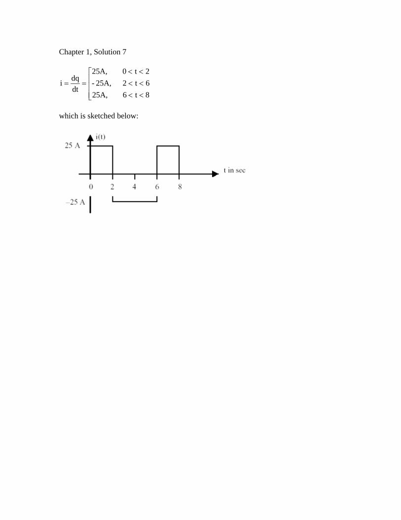
Chapter 1, Solution 7

8t6 25A,

6t2 25A,-

2t0 A,25

dt

dqi

which is sketched below:

Chapter 1, Solution 8

C 15 μ1102

110idtq

Chapter 1, Solution 9

(a) C 10 1

0dt 10idtq

(b)

C5.2255.715

152

1510110idtq

3

0

(c) C 30 101010idtq5

0

Chapter 1, Solution 10

q = it = 10x103x15x10-6 = 150 mC

Chapter 1, Solution 11

q= it = 90 x10-3 x 12 x 60 x 60 = 3.888 kC E = pt = ivt = qv = 3888 x1.5 = 5.832 kJ

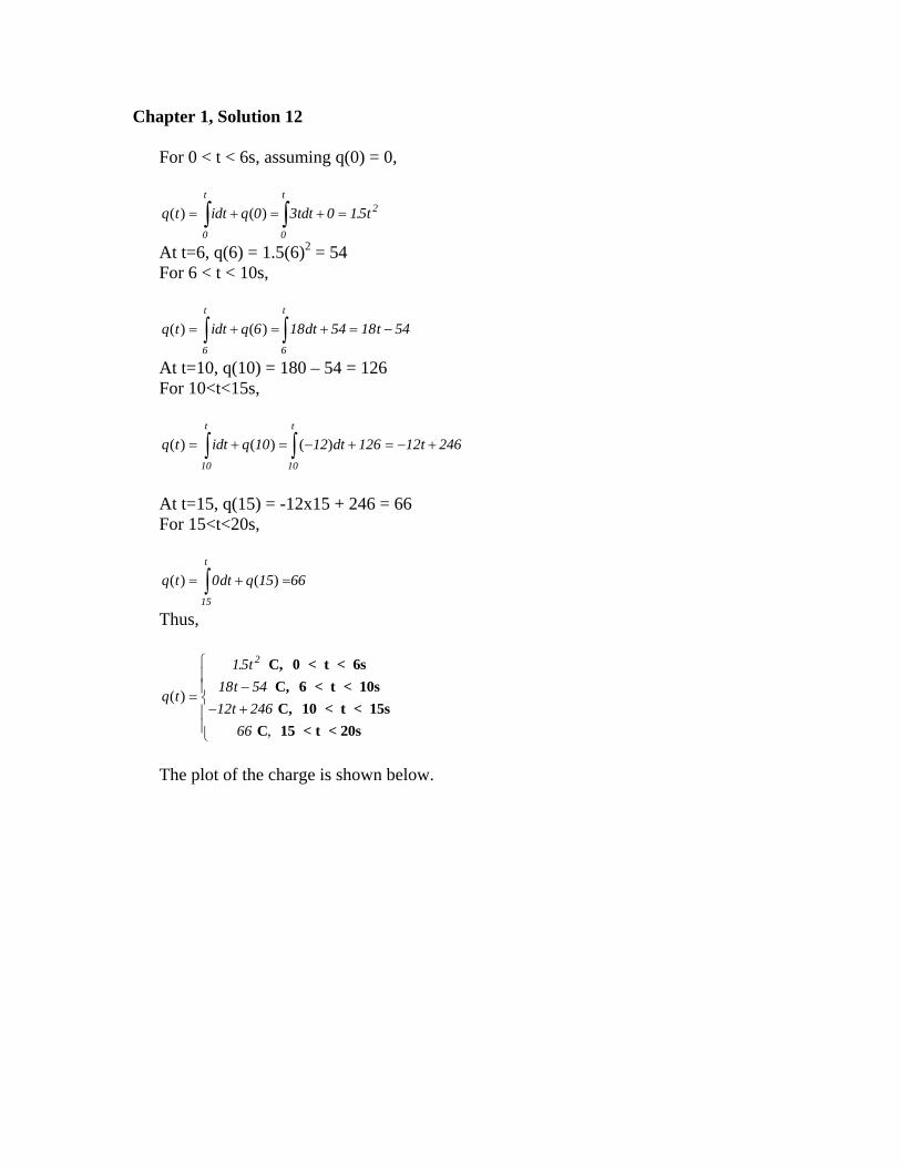
Chapter 1, Solution 12

For 0 < t < 6s, assuming q(0) = 0,

q t idt q tdt tt t

( ) ( ) . 0 3 0 150

2

0

At t=6, q(6) = 1.5(6)2 = 54 For 6 < t < 10s,

q t idt q dt tt t

( ) ( ) 6 18 54 18 56 6

4

66

At t=10, q(10) = 180 – 54 = 126 For 10<t<15s,

q t idt q dt tt t

( ) ( ) ( ) 10 12 126 12 24610 10

At t=15, q(15) = -12x15 + 246 = 66 For 15<t<20s,

q t dt qt

( ) ( ) 0 1515

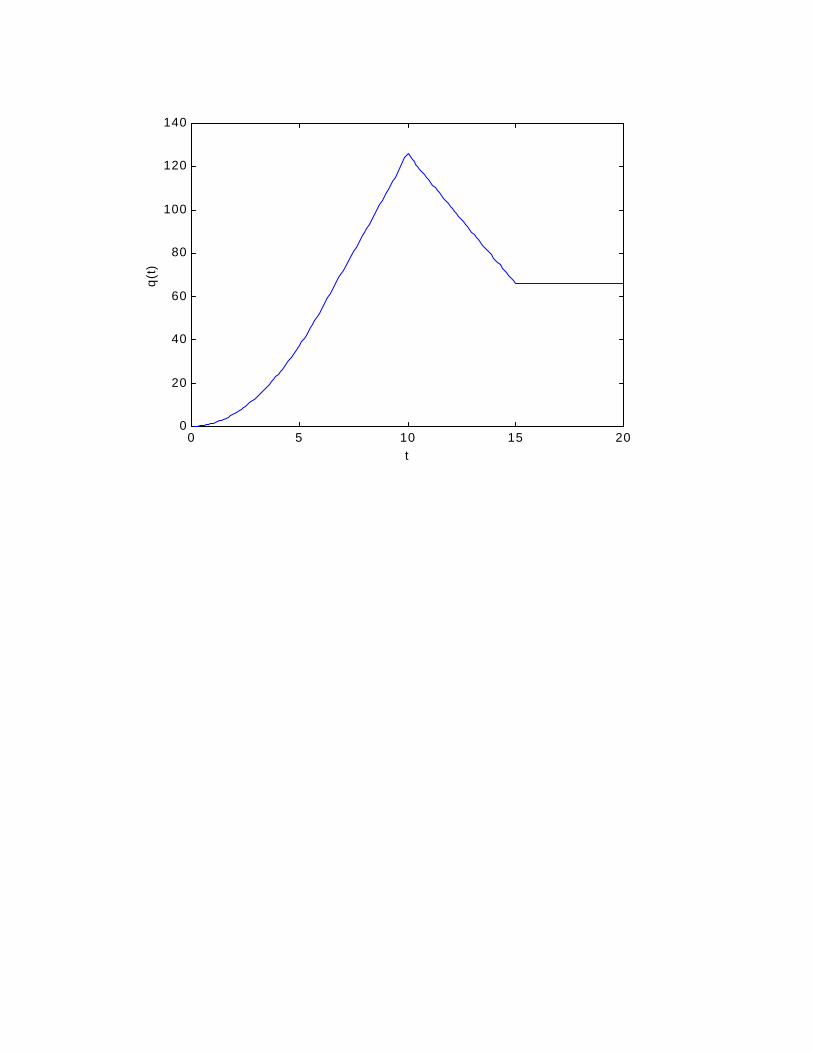
Thus,

q t

t

t

t( )

.

,

15

18 54

12 246

66

2 C, 0 < t < 6s

C, 6 < t < 10s

C, 10 < t < 15s

C 15 < t < 20s

The plot of the charge is shown below.

0 5 10 15 200

20

40

60

80

100

120

140

t

q(t

)

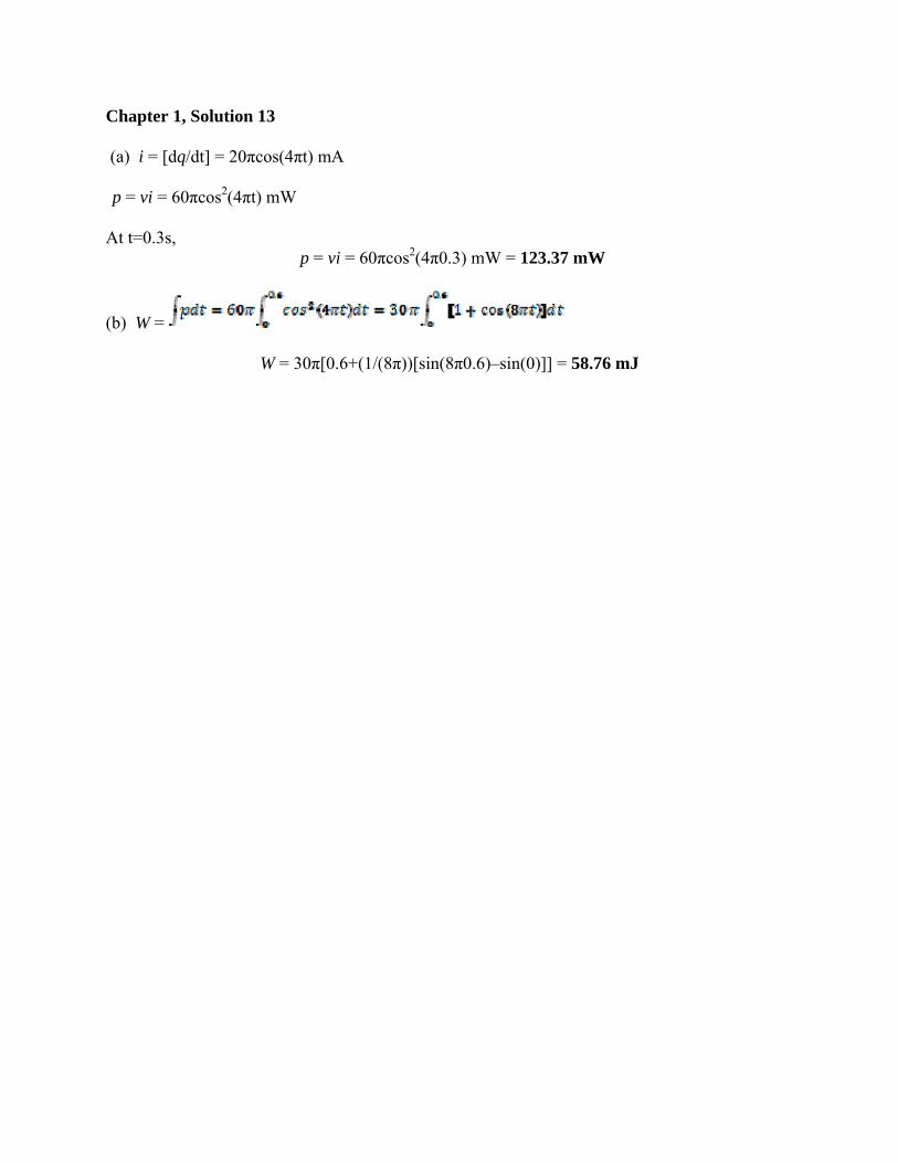
Chapter 1, Solution 13 (a) i = [dq/dt] = 20πcos(4πt) mA p = vi = 60πcos2(4πt) mW

At t=0.3s,

p = vi = 60πcos2(4π0.3) mW = 123.37 mW

(b) W =

W = 30π[0.6+(1/(8π))[sin(8π0.6)–sin(0)]] = 58.76 mJ

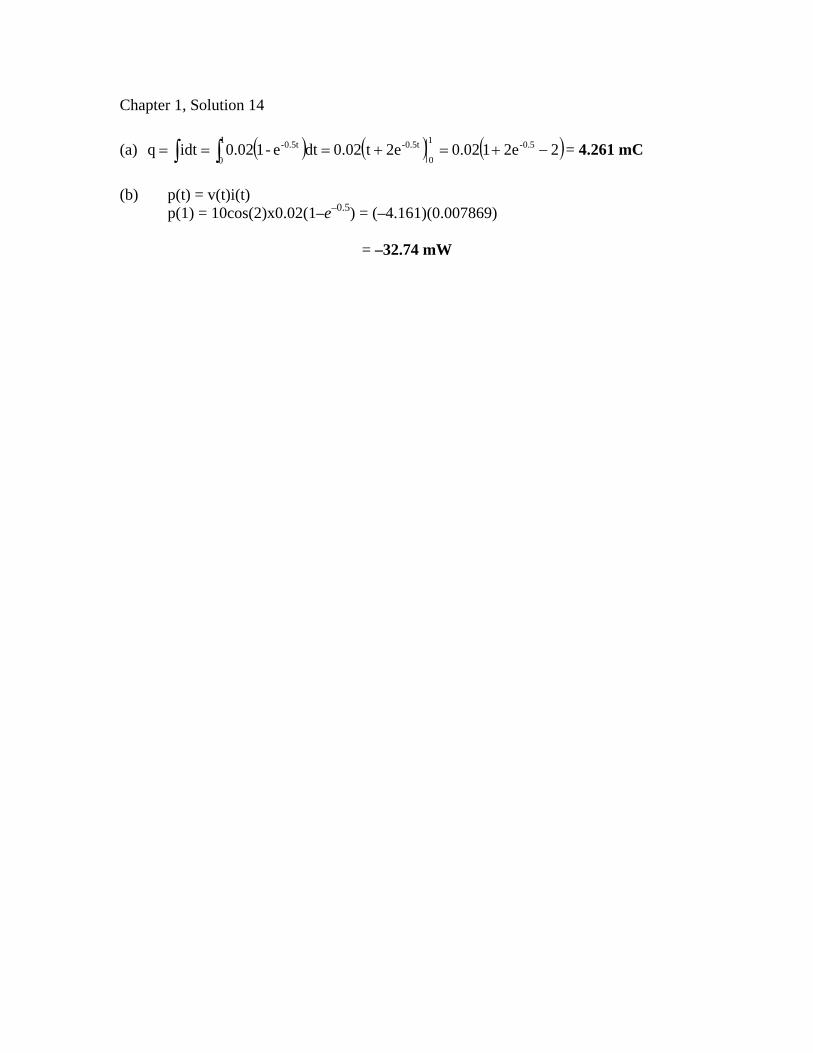
Chapter 1, Solution 14

(a) 2e2102.02et02.0dte-10.02idtq 0.5-1

0

0.5t-1

0

0.5t- = 4.261 mC

(b) p(t) = v(t)i(t) p(1) = 10cos(2)x0.02(1–e–0.5) = (–4.161)(0.007869)

= –32.74 mW

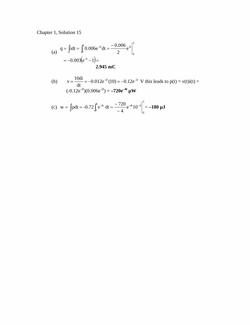
Chapter 1, Solution 15

(a)

1e003.0

e2

006.0dt0.006eidtq

4-

2

0

2t2

0

2t-

2.945 mC

(b) 2t-2t- e12.0)10(e012.0dt

di10v V this leads to p(t) = v(t)i(t) =

(-0.12e-2t)(0.006e-2t) = –720e–4t µW

(c) 3

0

64t-3

0

4t- 10e4

720dt e-0.72pdtw

= –180 µJ

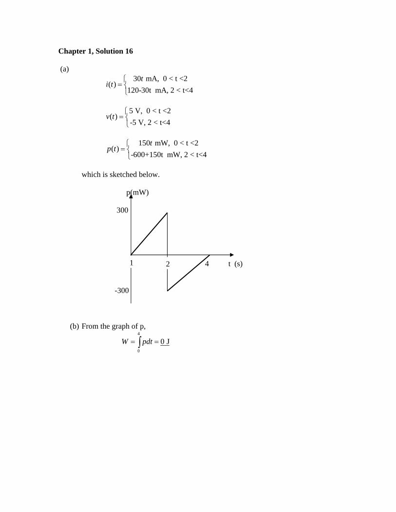
Chapter 1, Solution 16 (a)

30 mA, 0 < t <2( )

120-30t mA, 2 < t<4

ti t

5 V, 0 < t <2

( )-5 V, 2 < t<4

v t

150 mW, 0 < t <2

( )-600+150t mW, 2 < t<4

tp t

which is sketched below.

p(mW) 300 4 t (s) -300

1 2

(b) From the graph of p,

4

0

0 JW pdt

Chapter 1, Solution 17

p = 0 -205 + 60 + 45 + 30 + p3 = 0 p3 = 205 – 135 = 70 W Thus element 3 receives 70 W.

Chapter 1, Solution 18

p1 = 30(-10) = -300 W p2 = 10(10) = 100 W p3 = 20(14) = 280 W p4 = 8(-4) = -32 W p5 = 12(-4) = -48 W

Fundamentals Of Electric Circuits 5th Edition Alexander Solutions ManualFull Download: https://testbanklive.com/download/fundamentals-of-electric-circuits-5th-edition-alexander-solutions-manual/

Full download all chapters instantly please go to Solutions Manual, Test Bank site: TestBankLive.com