framework for calibration of a traffic state space model€¦ · 7.2.1 local and source alternating...

Department of Science and Technology Institutionen för teknik och naturvetenskap Linköping University Linköpings universitet

gnipökrroN 47 106 nedewS ,gnipökrroN 47 106-ES

LiU-ITN-TEK-A--12/070--SE

Framework for Calibration of aTraffic State Space Model

Magnus Fransson

Mats Sandin

2012-10-17

LiU-ITN-TEK-A--12/070--SE

Framework for Calibration of aTraffic State Space Model

Examensarbete utfört i Transportsystemvid Tekniska högskolan vid

Linköpings universitet

Magnus FranssonMats Sandin

Handledare David GundlegårdExaminator Clas Rydergren

Norrköping 2012-10-17

Upphovsrätt

Detta dokument hålls tillgängligt på Internet – eller dess framtida ersättare –under en längre tid från publiceringsdatum under förutsättning att inga extra-ordinära omständigheter uppstår.

Tillgång till dokumentet innebär tillstånd för var och en att läsa, ladda ner,skriva ut enstaka kopior för enskilt bruk och att använda det oförändrat förickekommersiell forskning och för undervisning. Överföring av upphovsrättenvid en senare tidpunkt kan inte upphäva detta tillstånd. All annan användning avdokumentet kräver upphovsmannens medgivande. För att garantera äktheten,säkerheten och tillgängligheten finns det lösningar av teknisk och administrativart.

Upphovsmannens ideella rätt innefattar rätt att bli nämnd som upphovsman iden omfattning som god sed kräver vid användning av dokumentet på ovanbeskrivna sätt samt skydd mot att dokumentet ändras eller presenteras i sådanform eller i sådant sammanhang som är kränkande för upphovsmannens litteräraeller konstnärliga anseende eller egenart.

För ytterligare information om Linköping University Electronic Press seförlagets hemsida http://www.ep.liu.se/

Copyright

The publishers will keep this document online on the Internet - or its possiblereplacement - for a considerable time from the date of publication barringexceptional circumstances.

The online availability of the document implies a permanent permission foranyone to read, to download, to print out single copies for your own use and touse it unchanged for any non-commercial research and educational purpose.Subsequent transfers of copyright cannot revoke this permission. All other usesof the document are conditional on the consent of the copyright owner. Thepublisher has taken technical and administrative measures to assure authenticity,security and accessibility.

According to intellectual property law the author has the right to bementioned when his/her work is accessed as described above and to be protectedagainst infringement.

For additional information about the Linköping University Electronic Pressand its procedures for publication and for assurance of document integrity,please refer to its WWW home page: http://www.ep.liu.se/

© Magnus Fransson, Mats Sandin

Framework for Calibration of a Traffic State

Space Model

Magnus Fransson, Mats Sandin

November 9, 2012

Copyright

The publishers will keep this document online on the Internet – or its possiblereplacement –from the date of publication barring exceptional circumstances.

The online availability of the document implies permanent permission foranyone to read, to download, or to print out single copies for his/hers own useand to use it unchanged for non-commercial research and educational purpose.Subsequent transfers of copyright cannot revoke this permission. All other usesof the document are conditional upon the consent of the copyright owner. Thepublisher has taken technical and administrative measures to assure authentic-ity, security and accessibility.

According to intellectual property law the author has the right to be men-tioned when his/her work is accessed as described above and to be protectedagainst infringement.

For additional information about the Linkoping University Electronic Pressand its procedures for publication and for assurance of document integrity,please refer to its www home page: http://www.ep.liu.se/.

c©Magnus Fransson & Mats Sandin

Abstract

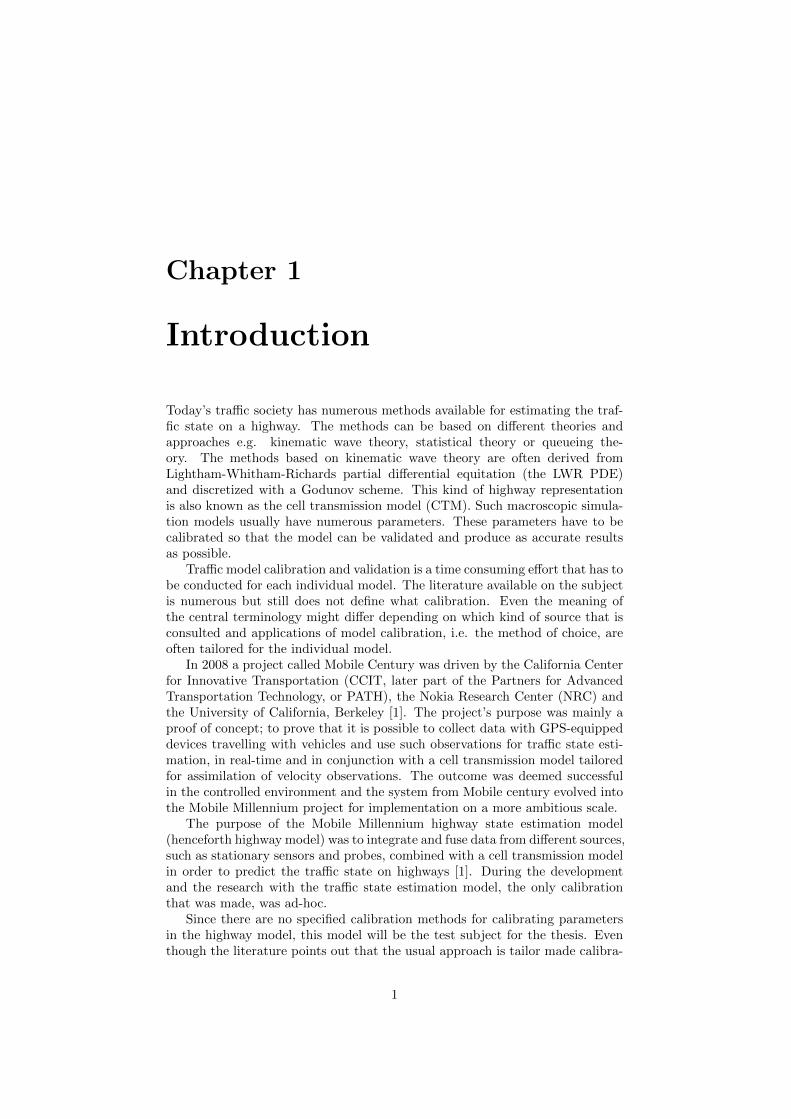
To evaluate the traffic state over time and space, several models can be used.A typical model for estimating the state of the traffic for a stretch of road ora road network is the cell transmission model, which is a form of state spacemodel. This kind of model typically needs to be calibrated since the differentroads have different properties. This thesis will present a calibration frameworkfor the velocity based cell transmission model, the CTM-v.

The cell transmission model for velocity is a discrete time dynamical systemthat can model the evolution of the velocity field on highways. Such a modelcan be fused with an ensemble Kalman filter update algorithm for the purposeof velocity data assimilation. Indeed, enabling velocity data assimilation wasthe purpose for ever developing the model in the first place and it is an essentialpart of the Mobile Millennium research project.

Therefore a systematic methodology for calibrating the cell transmission isneeded. This thesis presents a framework for calibration of the velocity basedcell transmission model that is combined with the ensemble Kalman filter.

The framework consists of two separate methods, one is a statistical ap-proach to calibration of the fundamental diagram. The other is a black boxoptimization method, a simplification of the complex method that can solveinequality constrained optimization problems with non-differentiable objectivefunctions. Both of these methods are integrated with the existing system, yield-ing a calibration framework, in particular highways were stationary detectorsare part of the infrastructure.

The output produced by the above mentioned system is highly dependenton the values of its characterising parameters. Such parameters need to becalibrated so as to make the model a valid representation of reality. Modelcalibration and validation is a process of its own, most often tailored for theresearchers models and purposes.

The combination of the two methods are tested in a suit of experiments fortwo separate highway models of Interstates 880 and 15, CA which are evaluatedagainst travel time and space mean speed estimates given by Bluetooth detectorswith an error between 7.4 and 13.4 % for the validation time periods dependingon the parameter set and model.

Acknowledgements

We are truly indebted to our mentor, friend and group leader Anthony D. Patirefor his help, patience and enthusiasm as well as for making our stay in Berkeleyone to remember.

We owe thanks to our mentors, Andreas Allstrom and David Gundlegard fortheir support and especially their trust and the amount of freedom that followedwith it.

For ever making this thesis possible we would like to thank our fellow internsand the staff at California Partners for Advanced Transportation Technology,especially Anastasios Kouvelas, Agathe Benoıt, Boris Prodhomme, Elie Daouand Jerome Thai. We hope that you have learned as much from us as we havefrom you.

We would like to thank our examiner, Clas Rydergren for his encouragementand for ever bringing the idea to do this thesis up to us.

Finally, our visit to University of California and California Partners for Ad-vanced Transportation Technology was made possible by financial support fromSweco Infrastructure.

We have truly seen a new world of opportunities, thank you all.

Contents

1 Introduction 11.1 Purpose and objectives . . . . . . . . . . . . . . . . . . . . . . . . 21.2 Method . . . . . . . . . . . . . . . . . . . . . . . . . . . . . . . . 21.3 Limitations . . . . . . . . . . . . . . . . . . . . . . . . . . . . . . 21.4 Outline . . . . . . . . . . . . . . . . . . . . . . . . . . . . . . . . 3

2 Literature Review Part I: Highway Model 42.1 Traffic flow model review . . . . . . . . . . . . . . . . . . . . . . 4

2.1.1 Transformation of the Lightham-Whitham-Richard par-tial differential equation . . . . . . . . . . . . . . . . . . . 5

2.1.2 Transformation to the velocity domain . . . . . . . . . . . 72.1.3 Discretization . . . . . . . . . . . . . . . . . . . . . . . . . 82.1.4 Fundamental diagrams . . . . . . . . . . . . . . . . . . . . 92.1.5 Cell transmission model for velocity . . . . . . . . . . . . 112.1.6 Model representation of junctions . . . . . . . . . . . . . . 122.1.7 Network algorithm . . . . . . . . . . . . . . . . . . . . . . 13

2.2 Data assimilation: The ensemble Kalman filter . . . . . . . . . . 142.2.1 Statistics . . . . . . . . . . . . . . . . . . . . . . . . . . . 142.2.2 Analysis schemes for combined model prediction and data

assimilation . . . . . . . . . . . . . . . . . . . . . . . . . . 202.2.3 Kalman filter . . . . . . . . . . . . . . . . . . . . . . . . . 262.2.4 Extended Kalman filter . . . . . . . . . . . . . . . . . . . 282.2.5 Ensemble Kalman filter . . . . . . . . . . . . . . . . . . . 30

2.3 Combining CTM-v and EnKF . . . . . . . . . . . . . . . . . . . . 362.3.1 Implementation of the CTM-v and EnKF combination . . 37

3 Literature Review Part II: Calibration 383.1 Calibration and validation of traffic models . . . . . . . . . . . . 38

3.1.1 Literature survey . . . . . . . . . . . . . . . . . . . . . . . 393.2 Automatic empirical calibration method . . . . . . . . . . . . . . 42

3.2.1 Regression analysis: Equality constrained least squares . . 433.2.2 Step I . . . . . . . . . . . . . . . . . . . . . . . . . . . . . 453.2.3 Step II . . . . . . . . . . . . . . . . . . . . . . . . . . . . . 453.2.4 Step III . . . . . . . . . . . . . . . . . . . . . . . . . . . . 463.2.5 Remarks . . . . . . . . . . . . . . . . . . . . . . . . . . . . 48

3.3 Complex method . . . . . . . . . . . . . . . . . . . . . . . . . . . 483.3.1 Formal presentation . . . . . . . . . . . . . . . . . . . . . 493.3.2 Example: Visualization of the complex movement . . . . 54

i

3.3.3 Example: Calibration of a single edge highway model . . 54

4 System Description 604.1 Overview . . . . . . . . . . . . . . . . . . . . . . . . . . . . . . . 604.2 Measurement loader . . . . . . . . . . . . . . . . . . . . . . . . . 614.3 Highway model . . . . . . . . . . . . . . . . . . . . . . . . . . . . 624.4 Ensemble Kalman filter revisited . . . . . . . . . . . . . . . . . . 62

5 Implementations of Calibration Procedures 645.1 Implementation of the automatic empirical calibration method . 64

5.1.1 Version I . . . . . . . . . . . . . . . . . . . . . . . . . . . 645.1.2 Version II . . . . . . . . . . . . . . . . . . . . . . . . . . . 675.1.3 Version III . . . . . . . . . . . . . . . . . . . . . . . . . . 695.1.4 Implementation remarks . . . . . . . . . . . . . . . . . . . 70

5.2 Link assignment . . . . . . . . . . . . . . . . . . . . . . . . . . . 715.2.1 Forward link assignment . . . . . . . . . . . . . . . . . . . 735.2.2 Backward link assignment . . . . . . . . . . . . . . . . . . 73

5.3 Complex method implementation . . . . . . . . . . . . . . . . . . 735.3.1 Ground truth . . . . . . . . . . . . . . . . . . . . . . . . . 745.3.2 Complex method: Implementation concept . . . . . . . . 765.3.3 Complex method: Implementation data flow . . . . . . . 805.3.4 Complex method: Simplification for problems with ex-

plicit constraints . . . . . . . . . . . . . . . . . . . . . . . 82

6 Experiments 846.1 Test site introduction . . . . . . . . . . . . . . . . . . . . . . . . 84

6.1.1 Test site I: Interstate 880, CA . . . . . . . . . . . . . . . . 846.1.2 Test site II: Interstate 15 Ontario . . . . . . . . . . . . . . 85

6.2 Experiment layout: Fundamental diagram estimation . . . . . . . 866.3 Experiment layout: Automated calibration . . . . . . . . . . . . 87

6.3.1 Local and source alternating calibration framework usingstandard fundamental diagrams . . . . . . . . . . . . . . . 88

6.3.2 Global and type-differentiated calibration framework us-ing estimated fundamental diagrams . . . . . . . . . . . . 90

6.3.3 Global calibration framework using estimated fundamen-tal diagrams . . . . . . . . . . . . . . . . . . . . . . . . . 91

7 Results 937.1 Fundamental Diagram Calibration Results . . . . . . . . . . . . . 937.2 Complex method calibration results . . . . . . . . . . . . . . . . 95

7.2.1 Local and source alternating calibration framework usingstandard fundamental diagrams: Interstate 880, CA . . . 95

7.2.2 Global and type-differentiated calibration framework us-ing estimated fundamental diagrams: Interstate 880, CA . 102

7.2.3 Global calibration framework using estimated fundamen-tal diagrams: Interstate 15, Ontario, CA . . . . . . . . . . 106

8 Analysis and Discussion 1138.1 Fundamental diagram estimation and link assignment procedure 113

8.1.1 Calibration framework . . . . . . . . . . . . . . . . . . . . 114

ii

9 Conclusion and Future Work 115

A Identified Parameters 119

B Bluetooth Deployment 126

C Fundamental Diagram Calibration Results 130

iii

List of Figures

2.1 Speed-density and flow-density relationships. . . . . . . . . . . . 92.2 Posterior probability. . . . . . . . . . . . . . . . . . . . . . . . . . 16

3.1 Flow-density measurements. . . . . . . . . . . . . . . . . . . . . . 433.2 Step I of Gunes’ method. . . . . . . . . . . . . . . . . . . . . . . 453.3 Step II of Gunes’ method. . . . . . . . . . . . . . . . . . . . . . . 463.4 Relationship between quartiles and mass of probability. . . . . . 473.5 Data-bin representation. . . . . . . . . . . . . . . . . . . . . . . . 473.6 Step III, and outcome, of Gunes’ method. . . . . . . . . . . . . . 483.7 Flowchart representation of the Complex method. . . . . . . . . . 533.8 Complex movement during optimization effort. . . . . . . . . . . 543.9 A highway section. . . . . . . . . . . . . . . . . . . . . . . . . . . 563.10 Weak boundary conditions. . . . . . . . . . . . . . . . . . . . . . 573.11 Example model output. . . . . . . . . . . . . . . . . . . . . . . . 583.12 Complex movement during calibration, a 3-dimensional case. . . 59

4.1 Data flow in the Mobile Millennium system. . . . . . . . . . . . . 61

5.1 Step I of Version I of the modified automatic empirical calibrationmethod. . . . . . . . . . . . . . . . . . . . . . . . . . . . . . . . . 65

5.2 Step II of Version I of the modified automatic empirical calibra-tion method. . . . . . . . . . . . . . . . . . . . . . . . . . . . . . 66

5.3 Step III of Version I of the modified automatic empirical calibra-tion method. . . . . . . . . . . . . . . . . . . . . . . . . . . . . . 66

5.4 Step I of Version II of the modified automatic empirical calibra-tion method. . . . . . . . . . . . . . . . . . . . . . . . . . . . . . 68

5.5 Step II of Version II of the modified automatic empirical calibra-tion method. . . . . . . . . . . . . . . . . . . . . . . . . . . . . . 68

5.6 Step III of Version II of the modified automatic empirical cali-bration method. . . . . . . . . . . . . . . . . . . . . . . . . . . . . 69

5.7 Step IV of Version III of the modified automatic empirical cali-bration method. . . . . . . . . . . . . . . . . . . . . . . . . . . . . 70

5.8 Link assignment procedure. . . . . . . . . . . . . . . . . . . . . . 725.9 Ground truth data collection. . . . . . . . . . . . . . . . . . . . . 755.10 Ground truth visualization. . . . . . . . . . . . . . . . . . . . . . 765.11 Layer view of the data processing. . . . . . . . . . . . . . . . . . 785.12 Layer view of parameter evaluation. . . . . . . . . . . . . . . . . 795.13 Feedback loop merged with the Mobile Millennium system’s data

flow. . . . . . . . . . . . . . . . . . . . . . . . . . . . . . . . . . . 81

iv

5.14 Flow chart of the simplified complex method. . . . . . . . . . . . 83

6.1 Overview of test site I: I-880 . . . . . . . . . . . . . . . . . . . . . 856.2 Overview of test site II: I-15 Ontario . . . . . . . . . . . . . . . . 86

7.1 Calibration framework 1: Initial validation of I-880 model. . . . . 967.2 Calibration framework 1: Validation of the initial calibration of

the I-880 model. . . . . . . . . . . . . . . . . . . . . . . . . . . . 977.3 Calibration framework 1: Initial validation of I-880 model, travel

time perspective. . . . . . . . . . . . . . . . . . . . . . . . . . . . 987.4 Calibration framework 1: Validation of the initial calibration of

the I-880 model, travel time perspective. . . . . . . . . . . . . . . 997.5 Calibration framework 1: Final model validation. . . . . . . . . . 1007.6 Calibration framework 1: Final model validation, travel time per-

spective. . . . . . . . . . . . . . . . . . . . . . . . . . . . . . . . . 1017.7 Calibration framework 1: Validation of the velocity field. . . . . . 1027.8 Calibration framework 2: Outcome of the calibration effort. . . . 1037.9 Calibration framework 2: Validation of the calibration effort. . . 1037.10 Calibration framework 2: Validation of the calibrated model,

travel time perspective. . . . . . . . . . . . . . . . . . . . . . . . 1057.11 Calibration framework 2: Validation of the velocity field. . . . . . 1067.12 Calibration framework 3: Model output prior to calibration. . . . 1077.13 Calibration framework 3: Validation of the calibration effort. . . 1077.14 Calibration framework 3: Model output prior to calibration. . . . 1087.15 Calibration framework 3: Validation of the calibration effort. . . 1087.16 Calibration framework 3: Validation of the calibration effort,

travel time perspective. . . . . . . . . . . . . . . . . . . . . . . . 1107.17 Calibration framework 3: Validation of the calibration effort,

travel time perspective. . . . . . . . . . . . . . . . . . . . . . . . 1117.18 Calibration framework 3: Validation of the velocity field. . . . . . 1127.19 Calibration framework 3: Validation of the velocity field. . . . . . 112

B.1 Overview of the I-880 Bluetooth deployment area. . . . . . . . . 126B.2 Detailed map over the I-880 Bluetooth deployment. . . . . . . . . 127B.3 Overview of the I-15 Ontario Bluetooth deployment area. . . . . 128B.4 Detailed map over the I-15 Ontario Bluetooth deployment. . . . 129

C.1 Space mean speeds on I-880 for different fundamental diagrams. . 130C.2 Space mean speeds on I-880 for different fundamental diagrams. . 131C.3 Space mean speeds on I-880 for different fundamental diagrams. . 131C.4 Space mean speeds on I-880 for different fundamental diagrams. . 132C.5 Space mean speeds on I-880 for different fundamental diagrams. . 132C.6 Space mean speeds on I-880 for different fundamental diagrams. . 133C.7 Space mean speeds on I-880 for different fundamental diagrams. . 133C.8 Space mean speeds on I-880 for different fundamental diagrams. . 134C.9 Space mean speeds on I-880 for different fundamental diagrams. . 134C.10 Space mean speeds on I-880 for different fundamental diagrams. . 135C.11 Space mean speeds on I-880 for different fundamental diagrams. . 135C.12 Space mean speeds on I-880 for different fundamental diagrams. . 136C.13 Space mean speeds on I-880 for different fundamental diagrams. . 136

v

C.14 Space mean speeds on I-15 Ontario for different fundamental di-agrams. . . . . . . . . . . . . . . . . . . . . . . . . . . . . . . . . 137












vi

List of Tables

3.1 Summary of the calibration and validation literature survey, macro-scopic models. . . . . . . . . . . . . . . . . . . . . . . . . . . . . . 41

3.2 Summary of the calibration and validation literature survey, mi-croscopic models. . . . . . . . . . . . . . . . . . . . . . . . . . . . 42

3.3 Parameter values retrieved from a calibration example using Gunes’method. . . . . . . . . . . . . . . . . . . . . . . . . . . . . . . . . 48

4.1 Summary of the measurement loader’s parameters. . . . . . . . . 614.2 Summary of the highway model’s parameters. . . . . . . . . . . . 624.3 Summary of the ensemble Kalman filter’s parameters. . . . . . . 63

5.1 Parameter results of Version I of the modified automatic empiricalcalibration method. . . . . . . . . . . . . . . . . . . . . . . . . . . 67

5.2 Parameter results of Version II of the modified automatic empir-ical calibration method. . . . . . . . . . . . . . . . . . . . . . . . 69

5.3 Parameter results of Version III of the modified automatic em-pirical calibration method. . . . . . . . . . . . . . . . . . . . . . . 70

6.1 Summary of the fundamental diagram calibration set-up. . . . . 87

7.1 RMSE-results for I-880 using different fundamental diagrams. . . 937.2 NRMSE-results for I-880 using different fundamental diagrams. . 947.3 RMSE-results for I-15 Ontario using different fundamental dia-

grams. . . . . . . . . . . . . . . . . . . . . . . . . . . . . . . . . . 947.4 NRMSE-results for I-15 Ontario using different fundamental di-

agrams. . . . . . . . . . . . . . . . . . . . . . . . . . . . . . . . . 957.5 MAPE of the travel time results after calibration of I-880. . . . . 1007.6 MAPE of the travel time results after calibration of I-880. . . . . 1047.7 MAPE of the travel time results after calibration of I-15 Ontario. 109

vii

Chapter 1

Introduction

Today’s traffic society has numerous methods available for estimating the traf-fic state on a highway. The methods can be based on different theories andapproaches e.g. kinematic wave theory, statistical theory or queueing the-ory. The methods based on kinematic wave theory are often derived fromLightham-Whitham-Richards partial differential equitation (the LWR PDE)and discretized with a Godunov scheme. This kind of highway representationis also known as the cell transmission model (CTM). Such macroscopic simula-tion models usually have numerous parameters. These parameters have to becalibrated so that the model can be validated and produce as accurate resultsas possible.

Traffic model calibration and validation is a time consuming effort that has tobe conducted for each individual model. The literature available on the subjectis numerous but still does not define what calibration. Even the meaning ofthe central terminology might differ depending on which kind of source that isconsulted and applications of model calibration, i.e. the method of choice, areoften tailored for the individual model.

In 2008 a project called Mobile Century was driven by the California Centerfor Innovative Transportation (CCIT, later part of the Partners for AdvancedTransportation Technology, or PATH), the Nokia Research Center (NRC) andthe University of California, Berkeley [1]. The project’s purpose was mainly aproof of concept; to prove that it is possible to collect data with GPS-equippeddevices travelling with vehicles and use such observations for traffic state esti-mation, in real-time and in conjunction with a cell transmission model tailoredfor assimilation of velocity observations. The outcome was deemed successfulin the controlled environment and the system from Mobile century evolved intothe Mobile Millennium project for implementation on a more ambitious scale.

The purpose of the Mobile Millennium highway state estimation model(henceforth highway model) was to integrate and fuse data from different sources,such as stationary sensors and probes, combined with a cell transmission modelin order to predict the traffic state on highways [1]. During the developmentand the research with the traffic state estimation model, the only calibrationthat was made, was ad-hoc.

Since there are no specified calibration methods for calibrating parametersin the highway model, this model will be the test subject for the thesis. Eventhough the literature points out that the usual approach is tailor made calibra-

1

tion methods for different models, this thesis will try to create a more generalframework. This framework should be able to be applied to other models thanthe highway model. This thesis will also present two procedures for calibratingdifferent types of parameters1.

1.1 Purpose and objectives

The purpose of this thesis is to develop a framework for calibrating a trafficstate space model. Since the definition of calibration and validation can differbetween articles, authors or other sources, it is required to define the conceptsof calibration and validation in this thesis.

The framework should fulfil some criteria. The second criteria is to providea general working process for how to calibrate and validate a traffic state spacemodel. It should also provide some calibration procedures as examples of howto estimate parameters connected to the model. Another purpose is to providesome results from calibrated test cases using the calibration framework for acertain traffic state estimation model and thereby validate the framework.

The objective with this thesis, is to produce a calibration framework fora traffic state estimation model. The framework should contain certain parts.The first part should be a general working process that describes the proce-dure in which the calibration should be made. It should also contain a generalcalibration procedure as well as a parameter specific procedure. Another aimis to measure and evaluate the performance of the traffic model when usingcalibrated parameter sets for the test sites.

1.2 Method

The two major approaches for developing and creating the framework was aliterature survey as well as a system analysis.

The literature survey was conducted as to bring in knowledge about the Mo-bile Millennium system, specifically the cell transmission model for velocity anddata assimilation with the ensemble Kalman filter. In parallel, the literaturesurvey also included the topics calibration, validation, empirical parameter esti-mation and black-box calibration so as to form the backbone of the calibrationframework.

Even though the framework as such can be used for other systems, it wasdeveloped for a specific traffic state space model, the Mobile Millennium system,being in the development stage and a large research topic at that, an extensivesystem analysis was needed. The primary goals for doing the analysis was tounderstand and identify all issues in the system. The analysis pointed out thatit was necessary to make modifications to the system, so that the system couldbe calibrated using the calibration framework.

1.3 Limitations

This thesis will mainly focus on two different calibration procedures for cali-brating parameters connected to the highway model. The two methods consists

1These procedures are exchangeable in the framework.

2

of a black box calibration method called the complex method and the other isan empirical calibration method for calibration of the parameters connected tothe fundamental diagram.

The data sources will be of three different kinds; probe data, inductive loopdetector data (from Caltrans Performance Measurement System, PeMS) andBluetooth data. Only limited data sets were available during the thesis. Pro-cessing of raw traffic data is outside the scope of this thesis although somequality assessment of filtered data will be conducted as part of the framework.

Due to lack of time, only two different calibration procedures was tested dur-ing the thesis in the frame work. Due to the factors mentioned, the performanceof the calibration procedures will not be compared against other calibrationmethods.

Only off-line calibration of parameters is addressed in this thesis. This meansthat the framework presents calibration methods that are used with historicaldata when calibrating parameters.

1.4 Outline

The outline for the rest of this thesis is as follows; first a literature review will bepresented in chapter. It consists of two chapters where the first chapter, chapter2, will focus on the transformation of the CTM to the CTM-v, the networkalgorithm and the theory behind the ensemble Kalman filter. The second part ofthe literature review, chapter 2, will focus on the theories behind the calibrationframework and calibration procedure. The purpose of the literature review isto present the theoretical foundation on which this thesis resides.

The following chapters will be the main contribution of this thesis. Chapter4, presents the system description, which have the purpose of presenting a moredetailed overview of the highway models and the relevant parameters connectedto each part. It will also present the data flow of the highway model. Afterthe system description, in 5, the implementation of the calibration frameworktogether with the calibration procedures chapter are introduced. These twochapters system description and the implementation chapter, describes for thereader how the author developed and adapted the calibration procedures andintegrated them into the highway model.

To prove that the calibration framework and the calibration procedures work,experiments are conducted. In chapter 6 the test sites, which is the subjectswhen conducting the experiments, as well as the layout are introduced andpresented. Chapter 7 summarizes and concludes the results from conductingthe experiments. The two last chapters in this thesis is the chapter 8 andchapter 9. Chapter 8 contains the analysis and discussion of the results fromthe work made. The final chapter which is chapter 9, concludes the work madein thesis and gives propositions for future work.

3

Chapter 2

Literature Review Part I:Highway Model

This chapter provides the literature review over the theoretical background forthe highway model in the Mobile Millennium system [2]. This highway modelis the traffic state space model that will be the experimental subject for thecalibration framework presented in this thesis. The chapter describes the math-ematics behind the highway model that lie within the scope of the thesis. Themain focus lie on derivatio of the velocity based cell transmission model and theensemble Kalman filter.

2.1 Traffic flow model review

This section will present a brief explanation to the Lightham-Whitham-Richard’s(LWR) kinematic wave theory with a small introduction to cell transmissionmodels (CTM), which is a recognized method for describing traffic states overtime and space. A review of different flux functions and the Godunov schemewill be presented. It will also introduce an inversion of the CTM into a velocitybased cell transmission model for which a network update algorithm is applied.

Macroscopic traffic models often use the CTM version from the Lightham-Whitham-Richard’s partial differential equation (LWR PDE). The theory wasdeveloped by Lightham, Whitham (1955), see [3] and Richards (1956), see [4].To express the flow as a function of density the PDE utilize a fundamentaldiagram. This diagram have evolved in many ways and there are different ver-sions. This report will give a brief explanation for three different fundamentaldiagrams; Greenshields [5], Daganzo-Newell [6] and the Hyperbolic-Linear fun-damental diagram and how they are connected to the LWR PDE.

The outline for the traffic model review section of this chapter is as follows.First a brief network representation to explain how a highway is simplified andmodelled. Thereafter an introduction to the theories behind the traffic flowmodel. Next, a transformation from the density domain to the velocity domainwill be introduced and explained. After a more detailed and link specific section,the cell transmission model for velocity (CTM-v) model is introduced. This kindof modelling are generally used to represent homogeneous stretches of road; anetwork representation these homogeneous stretches of road are defined as links.

4

To be able to extend the link modelling to a network representation, junctionsare introduced. The junctions acts as connection between links and distributesthe traffic flows over the outgoing links. Lastly, the network algorithm of howto estimate the state for the whole network is provided.

2.1.1 Transformation of the Lightham-Whitham-Richardpartial differential equation

In the LWR theory there is a partial differential equation known as the LWRPDE that expresses how the density ρ evolves for a certain stretch of road witha length of L, for a time period T . The LWR PDE is (2.1).{

∂ρ(x,t)∂t + ∂Qρ(x,t)

∂x = 0, (x, t)ε(0, L)× (0, T )

ρ(x, 0) = ρ0(x), ρ(0, t) = ρl(x), ρ(L, t) = ρr(x)(2.1)

where Q(·) is the fundamental digram1 for ρ ∈ [0, ρmax], where ρmax is themaximum density. Note that Q(·) often is assumed to be concave and piecewisedifferentiable. The initial condition, left boundary condition and right boundarycondition are expressed by the terms ρ0(·), ρl(·) and ρr(·). It is assumed thatthe flow can be described as (2.2).

Q = ρV (ρ) (2.2)

where the velocity V (·) is a function of the density ρ.To be able to characterize the behaviour of the LWR PDE correctly, under

the assumption that the desired density or measured density is not always equalto the modelled density gives that boundary conditions are needed to solvethe PDE. They can be either strong or weak, depending on how the network2

representation is formulated. The boundary conditions will be described moreclosely in the next part. Notations for the initial conditions as well as for theboundary conditions is as described above.

The initial boundary condition is directly corresponding to the density alongthe stretch of the modelled highway at time t = 0, this gives (2.3).

ρ(x, 0) = ρ0(x), x ∈ [0, L] (2.3)

where x is a specific stretch of road. In general, when trying to estimate thestate of a traffic system on a stretch of road, it is generally difficult to estimatethe initial conditions. To be able to cope with this problem, a system warmup can be used. By letting the system run over a sufficiently long time period,the significance of the initial conditions will be negligible. This is also calledthe flush out effect [2]. However, to solve (2.1) for the left and right boundaryconditions, [2] states that at least weak boundary conditions are used3. Byintroducing the weak boundary conditions, it is meant that the modelled density

1The fundamental digram express the relation between flow and density.2The network is a representation of the modelled highway, with junctions e.g. on and off

ramps.3By weak boundary conditions, it is meant that they are no longer required to hold abso-

lutely. In this way it is possible to use concepts from linear algebra to solve PDE:s. In thiscase it used to transform the PDE into an entropy function to be able to prove that a solutionexists.

5

and the desired density which is represented by ρ(l, t) = ρl(t) and ρ(r, t) = ρr(t)not always have to be absolute for all t.

According to [7] a simplification of the weak boundary conditions can beexpressed as (2.4) and (2.5). However for the mathematical specifics of thehyperbolic conservation law, which the LWR PDE is, the reader is referredto [8].

(I) ρ(l, t) = ρl(t) and Q′(ρl(t)) ≥ 0 or

(II) Q′(ρ(l, t)) ≤ 0 and Q′(ρl(t)) ≤ 0 or

(III) Q′(ρ(l, t)) ≤ 0 and Q′(ρl(t)) ≥ 0 and Q(ρ(l, t)) ≤ Q(ρl(t))

for all t

(2.4)and

(I) ρ(r, t) = ρr(t) and Q′(ρr(t)) ≤ 0 or

(II) Q′(ρ(r, t)) ≥ 0 and Q′(ρr(t)) ≥ 0 or

(III) Q′(ρ(r, t)) ≥ 0 and Q′(ρr(t)) ≤ 0 and Q(ρ(r, t)) ≤ Q(ρr(t))

for all t

(2.5)where Q′(·) = dq

dρ . Case (I) represents that the desired density is equal to

the modelled density. Case (II) represents the traffic state where both thedesired inflow as well as the modelled inflow, therefore the boundary condition ispushed by the current state. Case (III) represents that the boundary conditionis not able to push the inflow. This due to that the modelled density is incongestion and larger than the uncongested desired density. According to [7]this formulation ensures that it is possible to find an existing and unique entropysolution for a bounded domain.

So to be able to transform the density based CTM to a velocity based CTM-v it is needed to consider the density entropy solution, see (2.6), everything inline with [2]. This is also needed due to discontinuity that can appear in (2.1).The weak entropy solution for the density evolution model, the LWR PDE,can be written as (2.6). Note that earlier in the report, it is mentioned thatthe fundamental diagram is generally differential, piecewise linear and concave.However it is not possible to differentiate the Daganzo-Newell fundamental di-agram, which in turn rends it impossible to use in the entropy solution. It isa necessity that the fundamental diagram used in the entropy function can betwice differentiable (which the Daganzo-Newell digram is not) and is strictlyconcave with super linear growth. This is the motivation that [2] uses to intro-duce the hyperbolic-linear fundamental diagram.

L∫0

T∫0

(|ρ(x, t)− k| ∂

∂tϕ(x, t) + sgn(ρ(x, t)− k)(Q(ρ(x, t))−Q(k))

+∂

∂xϕ(x, t)

)dtdx+

L∫0

T∫0

sgn(k)(Q(Υρ(x, t))−Q(k)) · nϕ(x, t)dtdx ≥ 0

∀ϕ ∈ C2c ([0, L]× [0, T );R+), ∀k ∈ R

(2.6)

where Υ is the trace operator and n is the normal vector to the domain. Totransform the solution of the density based LWR PDE, which means that addi-tional boundary conditions for the initial conditions, left boundary conditions

6

and right boundary conditions is needed to be reformulated for this specific case.Not only in the weak sense but in a strong sense as well.

supk∈D(u(0,t),ul(t))

sgn(u(0, t)− ul(t))(F (u(0, t))− F (k)) = 0, a.e. t > 0. (2.7)

where D(x, y) = [inf(x, y), sup(x, y)]. 2.7 is the proper weak description for thetrace of the solution for u(0, t) and ul(t) for the left boundary condition of 2.1.

2.1.2 Transformation to the velocity domain

To be able to extend the LWR-v to a network model with proper boundary con-ditions, it is required to formulate them as strong boundary conditions insteadof weak conditions. In [2], they prove that the strong boundary conditions forthis case can be formulated as (2.8)-(2.9).

Q′(u(0, t)) ≥ 0 and Q′(ul(t)) ≥ 0

Q′(u(0, t)) ≤ 0 and Q′(ul(t)) ≤ 0 and u(0, t) = ul(t) xor

Q′(u(0, t)) ≤ 0 and Q′(ul(t)) > 0 and Q(u(0, t)) > Q(ul(t)) xor

a.t. t > 0

(2.8)and

Q′(u(L, t)) ≤ 0 and Q′(ur(t)) ≤ 0

Q′(u(L, t)) ≥ 0 and Q′(ur(t)) ≥ 0 and u(L, t) = ur(t) xor

Q′(u(L, t)) ≥ 0 and Q′(ur(t)) < 0 and Q(u(L, t)) > Q(ur(t)) xor

a.t. t > 0

(2.9)Note that u(·) is measured data, l and r is the boundaries, Q is the fundamentaldiagram and u(·, ·) is the solution.

Lastly, to be able to show that it is possible to recreate the LWR PDE for thevelocity domain with the same attributes as the density based LWR PDE, [2]introduces a modified velocity based entropy function that solves the PDE inits weak sense4, see (2.10).

L∫0

T∫0

(P (v(x, t))

∂ϕ

∂t(x, t) +Q(P (v(x, t)))

∂ϕ

∂x(x, t)

)dxdt

+

L∫0

P (v0(x))ϕ(x, 0)dx = 0, ∀ϕ ∈ C2c ([0, L]× [0, T ])

(2.10)

The first step to formulate the CTM-v, [2] wants to formulate the LWR-v PDEconservation law in the velocity based domain according to (2.11).

∂

∂tv(x, t) +

∂

∂xR(v(x, t)) = 0

v(x, 0) = v0(x)(2.11)

4By its weak sense, it is meant that a solution for the PDE cannot be guaranteed for thewhole domain.

7

where R(v) is a convex, velocity based fundamental diagram. Q = ρv is invert-ible, due to a strictly linear relationship.

This is done with the same approach as earlier, by introducing weak bound-ary conditions for the entropy function (2.10). The boundary conditions thenneeds to be reformulated, see (2.12) and (2.13) for (2.10).

u(0, t) = ul(t)

Q′(u(0, t)) ≤ 0 and Q′(ul(t)) ≤ 0 and u(0, t) 6= ul(t) xor

Q′(u(0, t)) ≤ 0 and Q′(ul(t)) > 0 and Q(u(0, t)) ≥ Q(ul(t)) xor

.

a.e. t > 0

(2.12)and

u(L, t) = ur(t)

Q′(u(L, t)) ≥ 0 and Q′(ur(t)) ≥ 0 and u(L, t) 6= ur(t) xor

Q′(u(L, t)) ≥ 0 and Q′(ur(t)) < 0 and Q(u(L, t)) ≥ Q(ur(t)) xor

.

a.e. t > 0

(2.13)where ul(·), ur(·) are of non differentiable functions. The functions ul(·) andur(·) strong boundary conditions applied to the left and right boundaries5.

2.1.3 Discretization

To discretize (2.13), [2] uses the Godunov scheme. This is a method to discretizethe LWR PDE and is commonly used in the traffic society. The Godunovscheme is a numerical approximation to the weak solution of the PDE in itsconservative form. It discretize the PDE in both time and space. In otherwords, by applying the Godunov scheme it is possible to reformulate the LWR-v PDE as a non-linear, dynamic system that is discrete in space and time. Inother words, the cell transmission model. To ensure numerical stability, it is

required that vmax∆T

∆x≤ 1, where vmax is the maximum modelled velocity. In

the descretization, the space step i ∈ {0, · · · , imax} with length ∆x is introducedas well as the time step n ∈ {0, · · · , nmax} with length ∆T . (2.14) is the celltransmission function for the LWR PDE.

ρn+1i = ρni −

∆T

∆X(G(ρni , ρ

ni+1)−G(ρni−1, ρ

ni )) (2.14)

where ρ is the density and G(ρ1, ρ2) is the Godunov density flow function, wherethe Godunov velocity flow function is defined as (2.15).

G(ρ1, ρ2) =

Q(ρ2) if ρcr ≤ ρ2 ≤ ρ1Q(ρcr) if ρ2 ≤ ρcr ≤ ρ1Q(ρ1) if ρ2 ≤ ρ1 ≤ ρcrmin

(Q(ρ1), Q(ρ2)

)if ρ1 ≤ ρ2

(2.15)

where Q(·) is the fundamental diagram, ρ1 is the upstream density and ρ2 isthe downstream density.

Since (2.14) is for estimating the traffic state for a certain cell in a certaintime step using density, a transformation to the velocity domain is needed. The

5This to ensure that a solution to the PDE can be found.

8

inversion is made by stating that Q(ρ) = Q(v) = V −1(v)v. It is possible ifV (·) is strictly decreasing and ρ1 ≤ ρ2 while v1 = V (ρ1) and v2 = V (ρ2) andv1 ≤ v2, where v1 is the upstream velocity and v2 is the downstream velocity. Itis also required that V (·) is monotonically decreasing and invertible. By usingthis statement, the relationship Q(ρ) = Q(v) = V −1(v)v can be assumed. Byinverting (2.14) and transforming (2.15), results in the velocity based cell trans-mission model, the CTM-v, see (2.16) and (2.17). Note that if the fundamentaldiagram is not affine, the inversion is needed to be made after the discretizationto yield the CTM-v.

vn+1i = V

(V −1vni −

∆T

∆x

(G(vni , v

ni+1)− G(vni−1, v

ni )))

(2.16)

where the Godunov velocity flow G(v1, v2) is given by (2.17).

G(v1, v2) =

Q(v2) if vcr ≤ v2 ≤ v1Q(vcr) if v2 ≤ vcr ≤ v1Q(v1) if v2 ≤ v1 ≤ vcrmin

(Q(v1), Q(v2)

)if v1 ≤ v2

(2.17)

2.1.4 Fundamental diagrams

This section will provide an introduction to the Greenshields [5], Daganzo-Newell [6] and the Hyperbolic-Linear fundamental diagram. It will also providethe inversion of the Hyperbolic-Linear fundamental diagram [2], which is laterused in the CTM-v.

vf

qmax

II.

ρcr ρmax

v

vf

vcr

ρ

q

I.

ρcr ρmax

vfvcr

III.

ρcr ρmax

1

Figure 2.1: Three different fundamental diagrams is pairwise shown inthis figure. The first pair I is the Greenshields fundamental diagram wherethe upmost diagam is represented in the velocity density domain and thelower is represented in the flow density domain. The second pair is theDaganzo-Newell fundamental digram and the third pair is the Hyperbolic-Linear fundamental diagram.

9

Greenshields fundamental diagram

The Greenshields fundamental diagram was invented by Bauce D. Greenshieldsin 1934. It was observed that the speed depended on the density. In [5], theystate the affine velocity function as (2.18). It expresses a linear relationshipbetween speed and density.

v = VG(ρ) = vmax

(1− ρ

ρmax

)(2.18)

where v is the estimated velocity and ρ is the density, G is a notation forGreenshields fundamental diagram, in graphical representation, see figure 2.1.

Daganzo-Newell fundamental diagram

In July 1993, Carlos F. Daganzo presented a cell transmission model in [9], asa dynamic representation of highway traffic. In this article, instead of using theGreenshields fundamental diagram, the author presents another fundamentaldiagram, see figure 2.1. A triangular where the differentiation between thecongested regime and the uncongested regime is strengthened. The fundamentaldiagram is expressed by (2.19).

v = VDN (ρ)

vmax, if ρ ≤ ρcr−wf

(ρmax

ρ

), otherwise

(2.19)

where vmax is the maximum velocity (free flow velocity), ρmax is the maxi-mum density, wf is the backward propagating shock wave velocity and DNis a notation for Daganzo-Newell fundamental diagram. The Daganzo-Newellfundamental diagram is not invertible since it is not strictly monotonic in freeflow.

Hyperbolic-Linear fundamental diagram

The main reason to why the Hyperbolic-Linear fundamental diagram is intro-duced is that the Daganzo-Newell fundamental diagram is not invertible. So theHyperbolic-Linear fundamental diagram is a combination between the Green-shields and the Daganzo-Newell fundamental diagram. For the mathematicalexpression of the Hyperbolic-Linear, see (2.20) and for graphical presentationsee 2.1.

v = VHL(ρ) =

vmax

(1− ρ

ρmax

), if ρ ≤ ρcr

−wf(

1− ρmax

ρ

), otherwise

(2.20)

where ρmax is the maximum density, ρcr is the critical density, wf is the back-ward propagating shock wave velocity, vmax is the free flow velocity and HLstands for that this fundamental diagram is the Hyperbolic-Linear fundamentaldiagram.

Since the system requires that everything should be expressed in the velocitydomain, an inversion of the Hyperbolic-Linear fundamental diagram is needed.

10

To be able to invert the fundamental diagram, continuity is required, especiallywhere ρ = ρcr. To achieve this, the authors in [2] introduce the continuityconstraint 2.21.

ρcrρmax

=wfvmax

(2.21)

After the continuity constraint is introduced, it is possible to invert (2.21), andthe inverted fundamental diagram is formulated as 2.22.

2.1.5 Cell transmission model for velocity

This section presents a summary of the CTM-v model proposed by [2] as wellas all the reasoning previously made. Just as for the network representation, alldeclarations are in line with those of [2]. To express the density as a functionof speed (2.22) is used.

ρ = V −1HL (v) =

ρmax

(1− v

vmax

), if v ≥ vcr

ρmax

(1

1 + vwf

), otherwise

(2.22)

In (2.22), V −1HL (v) denotes the inverted Hyperbolic-Linear velocity function,which is the inverse function of the approximated Daganzo-Newell velocity func-tion (see e.g. [2] for details). ρ is the vehicle density, v is the velocity, ρmax is themaximum, or jam, density, vmax is the free flow speed, vcr is the critical velocitycorresponding to the critical density vcr and wf is the backwards propagatingshock wave velocity.

The predicted velocity in the next time step for cell i is calculated via (2.23).This expression is what is called the Cell Transmission Model for velocity, orCTM-v.

vn+1i = V

(V −1(vni )− ∆T

∆x

(G(vni , v

ni+1)− G(vni−1, v

ni )))

(2.23)

where G is the transformed Godunov velocity flux.Transforming G and using (2.22), it is possible to yield the Hyperbolic-Linear

model (2.24).

G(v1, v2) =

Q(v2) = v2ρmax

(1

1 +v2wf

), if vcr ≥ v2 ≥ v1

Q(vcr) = vcrρmax

(1− vcr

vmax

), if v2 ≥ vcr ≥ v1

Q(v1) = v1ρmax

(1− v1

vmax

), if v2 ≥ v1 ≥ vcr

min(V −1HL (v1)v1V

−1HL (v2)v2

), if v1 ≥ v2

(2.24)

For the first and last cell however, the velocity at the next time step is calculatedwith (2.25) instead.

11

vn+10 = V

(V −1

(vn0

)− ∆T

∆x

(G(vn0 , v

n1

)− G

(vn−1, v

n0

)))vn+1imax

= V(V −1

(vnimax

)− ∆T

∆x

(G(vnimax

, vnimax+1

)−

G(vnimax−1, v

nimax

))) (2.25)

So at the boundaries of an edge, (2.23) will reference to points vn−1 and vnimax+1.These points are not within the physical domain, but are given by boundaryconditions. (2.24) can result in situations were the boundary conditions are notimposed on the physical domain.

2.1.6 Model representation of junctions

Physical restrictions requires that the flow distributions at the junctions aresolved. The first two restrictions (vehicle conservation and an imposed routingscheme) can be represented according to (2.26) and (2.27).∑

ein∈Ij

Qein(vein(Lein , t

))=

∑eout∈Oj

Qeout(veout

(0, t))

(2.26)

∑eout∈Oj

αj,eout,ein = 1 (2.27)

where αj,eout,ein is the allocation parameter and Aj ∈ [0, 1]|Oj |×|Ij | is the alloca-tion matrix for junction j. We also have the relations Aj(eout, ein) = αj,eout,einand αj,eout,ein ≥ 0. The purpose of the allocation parameters in the allocationmatrix is to distribute the traffic flow from the incoming edges to the outgoingedges according to routing information.

The restrictions expressed by (2.26) and (2.27) cannot always be fulfilledsince they combined impose strong boundary conditions at the end of the edges(note the equality). To solve this issue the third restriction is included (traf-fic flow is maximized over the junction) and the strong boundary conditionsrepresents upper bounds for that problem. The result is an optimization proce-dure (a LP-problem). The LP-problem solves the exiting flow on each incomingedge for the junction j. The dummy vector variable ξ ∈ R|Ij | is introduced forthe incoming edges ein of junction j. It is the possible to conclude the threerestrictions into the following LP-problem.

maximize: 1T ξ

Subject to: Ajξ ≤ γmaxOj

0 ≤ ξ ≤ γmaxIj

(2.28)

where the upper bounds are set by γmaxOj

:=(γmaxeout,1 , . . . , γ

maxeout,|Oj |

)and γmax

Ij :=(γmaxein,1 , . . . , γ

maxein,|Ij |

). The LP-problem expressed by (2.28) will have an optimal

solution ξ∗ for junction j. After estimating the maximum admissible outgoing

flux, it is possible to determine the state for G(vn−1, v

n0

)and G

(vnimax−1, v

nimax

)in (2.25) by (2.29).

12

Gein(vnimax, v

nimax+1

)= ξ∗ein ,

Geout

(vn−1, v

n0

)=

∑ein∈Ij

αj,eout,einξ∗ein

(2.29)

The maximum admissible outgoing and incoming maximum flow in (2.28) isdefined via (2.30) and (2.31) respectively.

γmaxeout

(veout(0, t)

)=

ρmax

(1− vcr,eout

vmax

)vcr,eout

if veout(0, t) ∈ [vcr,eout , vmax,eout ]

ρmax

(1

1+veout (0,t)

wf

)veout

(0, t)

if veout(0, t) ∈ [0, vcr,eout

]

(2.30)

and

γmaxein

(vein(Lein , t)

)=

ρmax

(1− vein (Lein

,t)

vmax

)vein(Lein , t)

if vein(Lein , t) ∈ [vcr,ein , vmax,ein ]

ρmax

(1

1+vcr,ein

wf

)vcr,ein

if vein(Lein , t) ∈ [0, vcr,ein ]

(2.31)

2.1.7 Network algorithm

The authors of [2], apart from deriving the CTM-v from the LWR PDE, definedan algorithm that progresses the velocity field in the network in time. The algo-rithm basically applies the CTM-v for each individual network edge and solvesthe LP-problem for each junction. The velocity field for the entire network, thatis, for every cell i ∈ {0, · · · , imax} on all edges, is

vn :=[vn0,e0 , · · · , vnimax,e0 , · · · , vn0,e|ε| , · · · , v

nimax,e|ε|

]The velocity at time t = (n+ 1)∆T is given by

vn+1 =M[vn] (2.32)

Where M[v] denotes the update algorithm presented below.

Step 1. For all junctions j ∈ J :

Compute γnimax,ein

(vnimax,ein

)∀ein ∈ Ij and

γn0,eout

(vn0,eout

)∀eout ∈ Oj using (2.30)-(2.31).

Solve the LP-problem (2.28) and update

Gein(vnimax

, vnimax+1

)and

Geout

(vn−1, v

n0

)using (2.29).

Step 2. For all edges e ∈ ε:Compute vn+1

i,e ∀i ∈ {1, · · · , imax,e}according to the CTM-v (2.23) and (2.25).

13

2.2 Data assimilation: The ensemble Kalmanfilter

One of the more noticeable features of the Mobile Millennium system is itsability to assimilate data in real time and offline mode from multiple sourcestogether with the highway model. This increases model performance in thesense that it becomes more knowledgeable about the true velocity state on theroad. This section will highlight the filtering technique that is used for dataassimilation in the Mobile Millennium system.

Evensen [10] presented a new method for sequential data assimilation, latercalled the ensemble Kalman filter, a variation of the Kalman filter which orig-inates from the 1960’s [11]. Evensen’s contribution was said to be a solutionto unwanted unbounded error growth in the extended Kalman filter, anotherversion of the Kalman filter, due to the simplifications in the error covarianceestimation [10]. Evensen used Monte Carlo methods to forecast the error statis-tics since the error covariance approximation in the extended Kalman filter wasdeemed to be to costly from a computational viewpoint but also because the newapproach would eliminate the unbounded error growth in the extended Kalmanfilter [10].

The main purpose of this section is to present the ensemble Kalman filter aswell as some background in statistics, data assimilation, the original Kalman fil-ter and the extended Kalman filter. This should make the reader aware of whatthese data assimilation techniques are, what an analysis scheme is, why neitherthe Kalman filter nor the extended Kalman filter can be used for data assimila-tion with the highway model update algorithm for velocity presented earlier andhighlight some important simplifications made in the extended Kalman filter.

The outline of the Data Assimilation: The ensemble Kalman filter sectionis as follows; the next section includes some background to statistics that iscarried throughout the description of Kalman filtering techniques. The bestpossible estimate of a state is then presented for circumstances where a priorstate and measurements of the true state are known. After the introduction tostate estimates with data assimilation the original Kalman filter is presented,followed by the extended Kalman filter and the ensemble Kalman filter. Theusual pattern in this section is that the presentation is done in a scalar case firstand them moved into a spatial domain.

2.2.1 Statistics

Before the Kalman filter or any of its variations are presented some statisticalterms and definitions upon which the data assimilation technique is foundedwill be presented.

Assume a random variable Ψ that is continuous over its domain. The ran-dom variable has an associated function F (ψ) which is known as a distributionfunction. This distribution function is defined as (2.33).

F (ψ) =

ψ∫−∞

f(ψ′) dψ′ (2.33)

where f(ψ) is a probability density function. f(ψ′) is therefore the change in

14

probability (density) and the distribution function F (ψ) states the cumulativeprobability that Ψ takes a value less than, or equal to ψ. As (2.33) is defined theprobability density function f(ψ) must be the first derivative of the distributionfunction F (ψ):

f(ψ) =∂F (ψ)

∂ψ(2.34)

The function f(ψ) expresses the probability of the random variable Ψ beingequal to ψ. Note that f(ψ) ≥ 0 always holds, that the probability of Ψ takinga value within a very small interval is equal to f(ψ)dψ on the one hand and onthe other hand that the probability of Ψ to take a value in ]−∞, ∞[ , is equalto one. The probability of Ψ being in an arbitrary interval [a, b] is defined by(2.35).

Pr(Ψ ∈ [a, b]) =

b∫a

f(ψ) dψ (2.35)

The probability distribution called the Gaussian (or normal) distribution iscommonly referred to in this thesis. The probability density functions for thesekinds of distributions are characterized by their variance σ2, mean value µ andare defined by (2.36).

f(ψ) =1

σ√

2πexp

(− (ψ − µ)2

2σ2

)(2.36)

Bayesian statistics in 2-dimensional spaces

Consider a case with two random variables Ψ and Φ. The joint probability den-sity function expresses the probability of Ψ and Φ occur together, this functionis denoted as f(ψ, φ). The conditional probability density function expressesthe probability of occurrence Ψ if occurrence Φ already took place, this functionis denoted f(ψ |φ) and is defined by (2.37).

f(ψ |φ) =f(ψ, φ)

f(φ)⇔ f(ψ, φ) = f(ψ |φ)f(φ) (2.37)

where

f(φ) =

∞∫−∞

f(ψ, φ)dψ (2.38)

Equation (2.37) states that f(ψ, φ) = f(ψ |φ)f(φ) where the right hand sideinterpreted as the likelihood Ψ given Φ times the probability of Φ. Note that ifthe occurrence Ψ is independent of the occurrence Φ and vice versa is the jointprobability density function f(φ, ψ) = f(φ)f(ψ).

Equation (2.37) gives Bayes’ theorem as (2.39) which states the conditional(after Φ) probability of Ψ which is more knowledgeable than the probability ofΨ alone since the data Φ now is taken into account.

f(ψ |φ) =f(ψ)f(φ |ψ)

f(φ)(2.39)

15

Consider Figure 2.2 below for example, before any information of the eventΦ is Pr(Ψ = ψ1) a volume that stretches the entire φ-space. This probability,or volume, considers the marginal distribution of Ψ alone and follows what iscalled a prior probability distribution. Assume now that Ψ and Φ are dependingevents and that information about the event (Φ = φ1) is known. This results ina conditional probability of Ψ given Φ expressed by a new intersection volumePr(Φ = φ1 ∩ Ψ = ψ1), a new probability following a posterior probability dis-tribution. According to the figure, the conditional probability can be expressedby (2.40).

Pr(Ψ = ψ1 |Φ = φ1) =Pr(Φ = φ1 ∩ Ψ = ψ1)

Pr(Φ = φ1)(2.40)

φ

ψf(ψ, φ)

ψ1

φ1

dφdψ

Pr(Φ = φ1 ∩ Ψ = ψ1)

Pr(Ψ = ψ1)

Figure 2.2: Visualization of Bayes’ theorem with a marginal distributionof only Ψ called a prior and a conditional distribution of Ψ given Φ calledthe posterior.

This knowledge about a prior and a posterior is important during the un-derstanding of the Kalman filtering techniques that are to be presented in thischapter. A good thought to keep track of is the idea of a model estimate as aprior while information about the true state through a field measurement allowsincreased knowledge of the true state.

Bayesian statistics in n-dimensional spaces

Since models which operates on n-dimensional spaces often are referred to inthis thesis, Bayesian statistics will be presented in a case more general than the2-dimensional one. Consider an event ψ ∈ <n, it has an associated functionF (ψ) and a probability density function f(ψ), which is also called the jointprobability density function for (ψ1, . . . , ψn). The associated function and theprobability density function are related according to (2.41) and the probability

16

density function is still the derivative of the associated function similar to (2.34).

F (ψ1, . . . , ψn) =

ψ1∫−∞

. . .

ψn∫−∞

f(ψ′1, . . . , ψ′n) dψ′1 . . . dψ

′n (2.41)

(2.35) is also true in the n-dimensional case, which means that the probabilityof ψ lying somewhere in <n is equal to one.

Consider the random variable ψ ∈ <n to be a model state which has anassociative function as well as a probability density function. In line with dataassimilation, introduce a measurement vector d holding measurement of the true(real world) state and let the likelihood of d given ψ be expressed by f(d |ψ).The joint probability density function of model state and measurements thenbecomes

f(ψ, d) = f(ψ)f(d |ψ) = f(d)f(ψ |d) (2.42)

The relationships given by (2.42) can, again, be used to express Bayes’ the-orem

f(ψ |d) =f(ψ)f(d |ψ)

f(d)(2.43)

which now expresses the model state probability density function with measure-ments, as a proportion to the probability density function of the model statealone times the likelihood for a certain set of measurements.

Two important statistical moments and covariance

Probability density functions have so far been introduced as functions that de-fines the probability of a random variable to take a certain value (see (2.35)).The probability density function contains information, such as its own expectedvalue µ, standard deviation σ and variance σ2.

The expected value for a function h(Ψ) where Ψ is a random variable is givenby (2.44).

E[h(Ψ)] =

∞∫−∞

h(ψ)f(ψ)dψ (2.44)

and the expected value of a random variable Ψ is then given by (2.45).

µΨ = E[Ψ ] =

∞∫−∞

ψf(ψ)dψ (2.45)

The expected value given by equations (2.44)-(2.45) expresses the expected av-erage value of Ψ if one performs an infinite number of realizations from thatdistribution.

The variance of a random variable Ψ is expressed by (2.46). This value statesthe spread of a probability distribution around the expected value.

σ2 = E[(Ψ − E[Ψ ])2] =

∞∫−∞

(ψ − E[Ψ ])2f(ψ)dψ = E[Ψ2]− E[Ψ ]2 (2.46)

17

(2.46) states that the variance is the expected square deviation of Ψ from theexpected value E[Ψ ], also known as the mean squared deviation.

Before moving on to estimation of statistics we present a measure, the covari-ance, which states how much two random variables Ψ and Φ follow one another.If a small Ψ corresponds to a small Φ this would give a positive covariance, asmall Ψ corresponding to a big Φ would give a negative covariance. The covari-ance for two random variables, for which the joint probability density functionis given by (2.37), is defined as (2.47).

Cov(Ψ, Φ) = E[(Ψ − E

[Ψ])(

Φ− E[Φ])]

= E[(ΨΦ− E

[Ψ]Φ− E

[Φ]Ψ + E

[Ψ]E[Φ])]

= E[ΨΦ]− E

[ΦE[Ψ]]− E

[ΨE[Φ]]

+ E[Ψ]E[Φ]

= E[ΨΦ]− E

[Ψ]E[Φ]− E

[Ψ]E[Φ]

+ E[Ψ]E[Φ]

= E[ΨΦ]− E

[Ψ]E[Φ]

=

∞∫−∞

∞∫−∞

ψφf(ψ, φ)dψdφ− E[Ψ]E[Φ]

(2.47)

Note in the last line of (2.47) that the probability density function f(ψ, φ) =f(ψ)f(φ) if Ψ and Φ are independent. In that case (2.47) is reduced to 0according to (2.48).

Cov(Ψ, Φ) =

∞∫−∞

∞∫−∞

ψφf(ψ, φ)dψdφ− E[Ψ]E[Φ]

=

∞∫−∞

∞∫−∞

ψφf(ψ)f(φ)dψdφ− E[Ψ]E[Φ]

=

∞∫−∞

φf(φ)( ∞∫−∞

ψf(ψ)dψ)dφ− E

[Ψ]E[Φ]

= E[Ψ] ∞∫−∞

φf(φ)dφ− E[Ψ]E[Φ]

= E[Ψ]E[Φ]− E

[Ψ]E[Φ]

= 0

(2.48)

Estimations from samples

As pointed out by [12], there is no practical way to make integrations as theones presented earlier in this chapter using a computer (performing numericalintegrations) if the dimensionality of the probability functions is high (i.e. > 3).

There is an alternative to numerical integrations called Markov Chain MonteCarlo methods in which a large number of realizations (draws), N , of the dis-tribution f(ψ) are known. Statistical moments can be estimated from suchsamples. In this section it will be shown how the expected value, µ, the vari-ance, σ2, and the covariance can be estimated from samples.

18

Assume a set {ψi} with i = 1, . . . , N where ψi is one observed value from thedistribution f(ψ), the expected value of a random variable from that distributioncan then be approximated by a best guess, the sample mean, according to:

µ = E[Ψ ] ' ψ =1

N

N∑i=1

ψi (2.49)

where the notation ' represents that the expected value of Ψ will tend to ψ asN → ∞. Note that ψ is an unbiased estimation of E[Ψ ], which is proven by(2.50).

E[ψ]

= E[n−1

N∑i=1

ψi]

=

N∑i=1

E[ψi]/n = nE[ψi]/n = E[Ψ ] (2.50)

The variance given by (2.46) can be approximated by the sample varianceaccording to (2.51).

σ2 = E[(Ψ − E[Ψ ]

)2]'(ψ − ψ

)2=

1

N − 1

N∑i=1

(ψi − ψ

)2 (2.51)

(2.51) is said to be an unbiased estimator of the variance. That the varianceestimator is unbiased means that it does not deviate from the expected variance.This can be proven by following the reasoning of (2.52).

ψi − ψ = (ψi − µ) + (µ− ψ)⇔(ψi − ψ)2 = (ψi − µ)2 + 2(ψi − µ)(µ− ψ) + (µ− ψ)2 ⇒

N∑i=1

(ψi − ψ)2 =

N∑i=1

(ψi − µ)2 + 2

N∑i=1

(ψi − µ)(µ− ψ) +

N∑i=1

(µ− ψ)2 ⇔

N∑i=1

(ψi − ψ)2 =

N∑i=1

(ψi − µ)2 + 2(µ− ψ)(

N∑i=1

ψi −Nµ) +N(µ− ψ)2 ⇔

N∑i=1

(ψi − ψ)2 =

N∑i=1

(ψi − µ)2 + 2(µ− ψ)(Nψ −Nµ) +N(µ− ψ)2 ⇔

N∑i=1

(ψi − ψ)2 =

N∑i=1

(ψi − µ)2 −N(ψ − µ)2 ⇔

N∑i=1

(ψi − ψ)2 = Nσ2 −N(σ)2/N

(2.52)

From which (2.51) can be deduced easily. Finally there is the covariance ofsamples defined as (2.53).

Cov(Ψ, Φ) = E[(Ψ − E

[Ψ])(

Φ− E[Φ])]

'(ψ − ψ

)(φ− φ

)=

1

N − 1

N∑i=1

(ψi − ψ

)(φi − φ

) (2.53)

19

This ends the introduction to statistics, presented thus far are the termsprobability density functions, accumulative probability functions and their prop-erties, Bayes’ theorem, the keywords prior and posterior, likelihood, expectedvalue, variance and covariance. It was also then proven that the expected value,the variance and the covariance can be estimated from samples.

This information will be used in the upcoming sections when state estimationby models and data assimilation is discussed.

2.2.2 Analysis schemes for combined model prediction anddata assimilation

The previous section introduced the notion of an available measurement d ofthe state. This section will bring together the measurement with the modelprediction in an effort to increase the performance of the state estimate, orrather minimize the difference between the true state and the state estimateproduced by the combined model prediction and measurement.

The outcome of this section should be awareness of what is commonly re-ferred to as the analysis scheme [12]. An analysis scheme is a way of combiningmodel predictions with field measurements where both the model state and themeasurement usually are dependent of time and space although this sectiondoesn’t include any time dependency.

The analysis scheme for a scalar state-space

Assume that the state at one specific location in space at one specific time is ψt

where the superscript t denotes true state. Now assume that two estimations ofψt are available. The first estimation is expressed by (2.54).

ψf = ψt + pf (2.54)

where the superscript f denotes forecast, or the prior estimate, or the first guess,of the true state and pf is the forecast error, ψf is then the state forecast.The estimate of the true state expressed by (2.54) is a model estimate unlikethe estimate expressed by (2.55) which is an measurement d which contains ameasurement error ε.

d = ψt + ε (2.55)

The task at hand is to find a new estimate ψa, the analysed estimate, which isa better estimate of ψt than both ψf and d. The issue is that, if new conditionsare imposed upon (2.54) in the form of the measurements d, the system will beoverdetermined [13]. The task at hand can then be reformulated to find a newestimate ψa that minimizes the error terms.

Assume that the error terms pf and ε are random variables with zero meansuch that:

pf = 0

ε = 0

(pf )2 = Cfψψ

ε2 = Cεε

(2.56)

20

where C denotes the covariance of the subscripted random variable pair. Assumea linear estimator such that:

ψa = ψt + pa = α1ψf + α2d (2.57)

I.e. ψa is a linear combination of the forecast and the measurement. Given(2.54) and (2.55) stating the model state forecast ψf and the measurement d(2.57) can be expressed as:

ψt + pa = α1ψf + α2d

= α1(ψt + pf ) + α2(ψt + ε)

= (α1 + α2)ψt + α1pf + α2ε

(2.58)

for which the expected value is used to find an expression for α1 and α2.

E[ψt + pa] = E[(α1 + α2)ψt + α1pf + α2ε]⇔

E[ψt] + E[pa] = (α1 + α2)E[ψt] + α1E[pf ] + α2E[ε]⇔E[ψt] + 0 = (α1 + α2)E[ψt] + α10 + α20⇔

E[ψt] = (α1 + α2)E[ψt]⇔1 = (α1 + α2)

(2.59)

With this result in mind (2.57) will be reduced according to (2.60):

ψa = α1ψf + α2d

= (1− α2)ψf + α2d

= ψf + α2(d− ψf )

(2.60)

It is also possible to deduce the error pa of the analyzed state ψa according to:

ψa = ψf + α2(d− ψf )⇔ψt + pa = ψt + pf + α2(ψt + ε− ψt − pf )⇔

pa = (1− α2)pf + α2ε

(2.61)

In which case the error variance of ψa, namely (pa)2, is expressed by (2.62).Note the assumption that the model and measurement errors are uncorrelated.

(ψa)2 = Caψψ =((1− α2)pf + α2ε

)2= (1− α2)2(pf )2 + 2α2(1− α2)pf ε+ α2

2ε2

=/pf ε = 0

/=

= (1− α2)2Cfψψ + α22Cεε

(2.62)

Since Cfψψ and Cεε are both positive and constant parameters the minimumvariance can be found by minimizing Caψψ with respect to α2:

dCaψψdα2

= 0⇔

0 = −2(1− α2)Cfψψ + 2α2Cεε ⇔

α2 =Cfψψ

Cfψψ + Cεε

(2.63)

21

The analyzed error variance is minimized for this choice of α2 and (2.60) becomes

ψa = ψf +Cfψψ

Cfψψ + Cεε(d− ψf ) (2.64)

And the error variance expressed by (2.62) becomes

Caψψ = Cfψψ

(1−

Cfψψ

Cfψψ + Cεε

)2

+ Cεε

(Cfψψ

Cfψψ + Cεε

)2

⇔

Caψψ = Cfψψ

(1−

Cfψψ

Cfψψ + Cεε

) (2.65)

(2.64) defines an unbiased and optimal estimation of a scalar state variable witha measurement and is an improved estimate of the state that includes both ofthe estimations given by (2.54) and (2.55).

The Bayesian analysis scheme for a scalar state-space

Returning to Bayesian statistics and the notion of prior and posterior estimates,assume an initial guess ψf for which there is a probability density function f(ψ).The likelihood of getting a measurement d given ψ is f(d |ψ) and it was shownpreviously that Bayes’ theorem gives f(ψ | d) ∝ f(ψ)f(d |ψ). The notation ∝means that the probability density function of ψ given d is proportional to theright hand side of that expression.

Assume that two estimates of the state similar to (2.54) and (2.55) areavailable and that all distributions are Gaussian (see (2.36)). The density of theprior estimate of the state is given by

f(ψ) ∝ exp(− 1

2(ψ − ψf )(Cfψψ)−1(ψ − ψf )

)(2.66)

while the likelihood of d given ψ, or simply the likelihood, is given by

f(d |ψ) ∝ exp(− 1

2(ψ − d)C−1εε (ψ − d)

)(2.67)

Considering (2.66)-(2.67) the posterior density can be expressed in the sameway as (2.43), which gives:

f(ψ | d) ∝ exp(− 1

2J [ψ]

)(2.68)

Where the operator J follows the notation of Evensen and shortens the expres-sion in (2.68) while being defined as equation (2.69) [12].

J [ψ] = (ψ − ψf )(Cfψψ)−1(ψ − ψf ) + (ψ − d)C−1εε (ψ − d) (2.69)

Since exp(−β) = 1/(eβ), a minimization of J with respect to ψ will give a

22

maximization of the posterior density in (2.68).

J [ψ] = (ψ − ψf )(Cfψψ)−1(ψ − ψf ) + (ψ − d)C−1εε (ψ − d)⇒

dJdψ

= 2(ψ − ψf )(Cfψψ)−1 + 2(ψ − d)C−1εε = 0⇔

ψ =ψfCεε + dCfψψ

Cfψψ + Cεε⇔

ψ = dCfψψ

Cfψψ + Cεε+ψfCεε + ψfCfψψ − ψfC

fψψ

Cfψψ + Cεε⇔

ψ = ψf +Cfψψ

Cfψψ + Cεε(d− ψf )

(2.70)

Where the last row is noted to be equivalent to the result of (2.64), so the likeli-hood maximization given by a variance minimization in the case with Gaussiandistributions for all error terms. It is always true that a minimum-variance esti-mate yields a maximum-likelihood estimate when the distributions are Gaussian.Note that this equivalence is not true for non-Gaussian distributions but that(2.69) still can be used to find the estimator that minimizes the variance [13].

The analysis scheme for spatial state-spaces

The previous section outlined the problem of combining modelled states withmeasurements of the same in a scalar case (a single location), this section willexpand this problem to a spatial domain (the whole length of a road for ex-ample). The task at hand is still to find a way of combining state estimatesgiven by a prediction model with those given by field measurements but now ina spatial domain, say x = (x, y, z) or a discrete spatial domain such as a cellrepresentation of a road. The outcome is an analysis scheme. It is used laterwhen the Kalman filter is presented.

Consider a variable ψf (x) expressing the first guess of the state at a locationx. Let d ∈ <M be a measurement vector with M measurements. Say that thesemeasurements can be mapped to the true state with M ∈ <M which is called ameasurement functional. The basic spatial formulation of the first guess of thestate expressed by (2.54) can then be expressed as

ψf (x) = ψt(x) + pf (x) (2.71)

while the measurement vector, that can be compared to (2.55), is

d = M[ψt(x)

]+ ε (2.72)

Both of (2.71) and (2.72) contains an error term with unknown values (otherwisewould the true state be known). Note that ε ∈ <M . Regarding the measurementfunctional can such an operator be

Mi

[ψ(x)

]=

∫Dψ(x)δ(x− xi)dx (2.73)

23

where δ is the delta function that is equal to zero for every x ∈ D except forx = xi. The subscript i is a measurement location index.

There is no way to do any further analysis about the state estimate in thespatial domain without making some assumptions about the error statistics,since no information about the errors pf (x) or ε is known [12]. Let the informa-tion in (2.56) be true in the spatial case . This means that both of the errors havea mean value equal to zero, and there is information present about the varianceof the measurement errors and there is knowledge about the covariance betweentwo spatial points xi and xj in the forecast step.

pf (x) = 0

ε = 0

pf (xi)pf (xj) = Cfψψ(xi, xj)

εεT = Cεε

(2.74)

where Cεε ∈ <M×M is a covariance matrix which is not to be confused with(2.53) since it is not deduced from sample averages but from the true state.

Given the statistical null hypothesis (2.74) the next step of the discussionis to define a function J that can be used to punish large deviations betweenthe state ψ and the model forecast ψf and the measurements d respectively.Evensen [12] stated (2.75) as an example of such a function. (2.75) contains twoterms. The first of those two terms states a weighted measurement between theforecast ψf (x) and the state estimate ψ(x). The second term measures (in aweighted fashion) the distance between the field measurement d and the stateestimate.

J [ψ] =

∫∫D

(ψf (x1)− ψ(x1)

)W fψψ(x1,x2)

(ψf (x2)− ψ(x2)

)dx1x2

+(d−M(3)[ψ3]

)TWεε

(d−M(4)[ψ4]

) (2.75)

W and W are the (functional) inverses of Cfψψ(x1, x2) and Cεε respectively,the subscripts of the expression M(i)[ψi] indicates dummy variables that areused later during the derivation of the analysis scheme [12]. The inverses of thecovariances are the weights mentioned earlier.

The function J [ψ] given by (2.75) will grow if the state estimate deviatesfrom the forecast state and the field measurements. It is therefore desirable tofind the optimal solution ψ(x) = ψa(x) that minimizes that expression. If theweights are inverses of error covariances following Gaussian distributions thevariance minima equals the likelihood maxima [12].

It can be proven that (2.76) is an optimal solution to (2.75) by deriving theEuler-Lagrange equation from δJ = J [ψ+ δψ]−J [ψ] = O(δψ2) [12]. The ideais to take the variational derivative of the variational functional J and assumethat J → 0 as δψ(x)→ 0.

ψa(x)− ψf (x) = MT(3)[C

fψψ(x,x3)]Wεε(d−M(4)[ψ

a4 ]) (2.76)

(2.76) is not a satisfactory solution to (2.75) since ψa is included in both theright hand side and the left hand side of the expression. It is more desirable tosearch for an expression for ψa such as the analysis

ψa(x) = ψf (x) + bTr(x) (2.77)

24

where

b = Wεε(d−M(4)[ψa4 ]) (2.78)

is a vector in <M . (2.77) can be proven to be a variance minimizing (optimal)which is both unique and linear [12]. r(x) are called representers. If (2.77) isinserted in the optimal solution given by (2.76) can it be shown that

r(x) = M(3)[Cfψψ(x,x3)] (2.79)

A different expression for the vector b can be deduced from (2.77)-(2.79) andis given by (2.80) [12].(

M(3)MT(4)[C

fψψ(x3,x4)] +Cεε

)b = d−M(4)[ψ

f (x4)] (2.80)

The missing piece is to derive an error estimate for (2.77) similar to the onedone for the scalar analysis scheme that was expressed by (2.65). This is donewith greater effort than for the scalar case and by taking the error covariancegiven by (2.74) which is

Caψψ(x1,x2) = (ψt(x1)− ψa(x1))(ψt(x2)− ψa(x2)) (2.81)

and substituting this expression in (2.77) which leads to (2.82) if the procedurepresented in Evensen [12] is followed.

Caψψ(x1,x2) = Cf

ψψ(x1,x2)

− rT (x1)(M(3)MT

(4)[Cfψψ(x3,x4)] +Cεε

)−1r(x2)

(2.82)

Formulation of the analysis scheme for discrete domains

The previous section outlined the analysis scheme in a spatial domain e.g. x =(x, y, z) which is continuous. It is usually desirable to make a vector or matrixrepresentation of the spatial domain that is modelled, so as to represent thedomain with a discrete numerical grid ψ. In that case (2.71) and (2.72) wouldbe

ψf = ψt + pf

d = Mψt + ε(2.83)

where ψ is a vector (numerical grid) representation of the spatial domain, pf

and ε are error terms in vector form, d is a measurement vector and M is adiscrete version of the measurement functional M, meaning that M is a matrixthat maps between the measurement vector and the state vector.

Similar to the procedure made in the previous sections it can be proven that(2.84) is an optimal solution to the minimized variational functional problem[12].

ψa = ψf + rT b (2.84)

where

r = MCfψψ (2.85)

25

is a matrix that holds the elements of the error covariance matrix at the spotsof the measurements.

The vector b in (2.84) can be derived from the discrete formulation of (2.80)which is given by (2.86).(

MCfψψMT +Cεε

)b = d−Mψf (2.86)

Finally there is the discrete formulation of the time evolution of the error statis-tics in the discrete case. The discrete formulation of (2.82) is

Caψψ = Cf

ψψ − rT(MCfψψM

T +Cεε

)−1r (2.87)

Looking back at this section it can be seen that the analysis scheme givesan estimate ψa of the true state ψt and that this estimate is composed by aninverse of the estimate ψf as well as a linear combination rT b which is just acollection of influence functions, the amount of which is equal to the number ofmeasurements [12]. Given the expression of b is it clear that b will be small ifthe forecast state ψf is close to the measurements d [12].

This concludes the introduction to analysis schemes, the introduction is usedin the coming section where the Kalman filter is presented and, through theKalman filter, is it also used when the extended Kalman filter and the ensembleKalman filter are presented.

It is important to note that the analysis scheme so far has been presented asbeing independent of time, the concept of a time dynamical scheme is introducedwith the Kalman filter. This presentation of the analysis scheme in scalar andspatial cases only regarded what was early on presented as a prior, or a forecast,ψf of the state and that a posterior, or the optimal conditional estimate, ψa

was computed once extra knowledge in the form of measurements d was broughtinto the picture.

2.2.3 Kalman filter

The previous section presented analysis schemes for time independent scalarand spatial cases. The discussion was oriented around the notions of a prior,or a forecast, and measurements of the state and how these two componentscould be combined to yield the optimal (the variance minimizing, or likelihoodmaximizing) state estimate ψa.

These analysis schemes can be used to perform sequential data assimilationand model state updates. As previously shown an improved state estimatein vector form ψa can be computed from the forecast ψf , the forecast errorcovariance matrix Cf

ψψ, the measurement vector d and the measurement errorcovariance matrix Cεε. These components can also be used to compute Ca

ψψ,the analyzed error covariance matrix.

This can be done in the time dynamic and discrete case, this section willoutline this process for linear time dynamical cases. It is referred to as theKalman filter.

The scalar case

Let G be a linear model operator that evolves the state ψtk = ψt(tk) in time,where tk is the kth time value. This time evolution process is expressed by the

26

time dynamical system

ψtk = Gψtk−1 + qk−1 (2.88)

with

ψt0 = Ψ0 + a (2.89)

where qk is a time dependent error term, Ψ0 is the initial state and ψt0 is thatsame initial state but including an error term a.

The true state estimation model cannot be expressed directly as equations(2.88) and (2.89), since the error qk, that could represent error sources such asmodel limitations, is unknown. Instead, the actual model is expressed as (2.90)and (2.91).

ψfk = Gψak−1 (2.90)

with

ψa0 = Ψ0 (2.91)

Equation (2.90) states the following: A forecast estimate of the state at timetk is given by integrating the best guess ψak−1 forward in time according to themodel operator G.

Since (2.88) is the true state and (2.90) is the best guess that can be made,

the forecast will have a state error (ψtk−ψfk ), which can be used to estimate theunknown error statistics:

ψtk − ψfk = G(ψtk−1 − ψak−1) + qk−1 (2.92)

In which case

Cfψψ(tk) = (ψtk − ψfk )

= (G(ψtk−1 − ψak−1) + qk−1)2

= G2(ψtk−1 − ψak−1)2 + 2G(ψtk−1 − ψak−1)qk−1 + q2k−1

(2.93)

Assuming that the model error qk and the state error (ψtk−ψfk ) are uncorrelated

is (ψtk−1 − ψak−1)qk−1 = 0, and (2.93) is reduced to

Cfψψ(tk) = G2(ψtk−1 − ψak−1)2 + 0 + q2k−1

= G2Caψψ(tk−1) + Cqq(tk−1)(2.94)

The model evolves in time as given by the dynamical equation (2.90) withstarting conditions given by (2.91). The model state error covariance Caψψ(tk−1),the model error covariance Cqq(tk−1) and the initial error covariance Cψψ(t0)evolves according to

Caψψ(tk−1) = (ψtk−1 − ψak−1)2 (2.95)

Cqq(tk−1) = (q2k−1) (2.96)

Cψψ(t0) = Caa = a2 (2.97)

Which then concludes the model evolution and the error covariance evolutionas a consistent time dynamical system.

When a measurement d is available the analysis scheme given by (2.64) willyield an analysed state estimate.

27

The vector case

The state in a spatial domain can be mapped to a discrete grid represented bythe elements in a state vector ψtk. With a linear model operator in matrix formthe true state vector representation will evolve according to

ψtk = Gψtk−1 + qk−1 (2.98)

where the variables follows the description of those in (2.88). The estimation of(2.98) is

ψfk = Gψak−1 (2.99)

The error covariance matrix Cfψψ(tk) can be found by a procedure similar to

the one used to find Cfψψ(tk) in (2.94).

Cfψψ(tk) = GCa

ψψ(tk−1)GT +Cqq(tk−1) (2.100)

The time evolution equations (2.99) and (2.100) together with the analysis equa-tions (2.101)-(2.103) is the Kalman filter [12,14].

ψak = ψfk +Kk(dk −Mkψfk ) (2.101)

where d is the measurement vector and M is a matrix that maps the statevector to the measurements, it is also known as a measurement matrix. Thecovariance matrix Ca

ψψ time evolution is given by

(Cψψ)ak = (I −KkMk)(Cψψ)fk (2.102)

Both of the equations (2.101) and (2.102) contains a matrix K, this matrix iscalled the Kalman gain and is given by

Kk = (Cψψ)fkMTk (Mk(Cψψ)fkM

Tk + (Cεε)k)−1 (2.103)

(2.101)-(2.103) are the more common way to post the analysis (or update) equa-tions of the Kalman filter than (2.84)-(2.87) and one of these equation sets canbe deduced directly from the other [12,14].

2.2.4 Extended Kalman filter

The previous section presented the Kalman filter, which produces the optimalstate estimate for linear functions G. In the case of non-linear functions Ghowever, the Kalman filter cannot be used directly. But if G is differentiablecan it be approximated by a Taylor expansion.

This section will briefly outline the extended Kalman filter for sequentialdata assimilation in which an estimate of the error covariance time evolution isused and for linear measurement operators.

The scalar case

Let (2.104) represent a time dynamical non-linear model of the state of a singlescalar value ψtk.

ψtk = G(ψtk−1) + qk−1 (2.104)

28

Just as in the previous section is it noted that the error q depends on e.g. modelinaccuracies and that q is unknown. Assume a numerical model of the state thatis approximated by:

ψfk = G(ψak−1) (2.105)

In which case the error between the models given as equations (2.104) and(2.105) is the difference

ψtk − ψfk = G(ψtk−1)−G(ψak−1) + qk−1 (2.106)

Assume that G is infinitely differentiable, the next step includes a Taylorexpansion of G(ψtk−1)) in the close proximity of ψak−1:

G(ψtk−1) = G(ψak−1) +G′(ψak−1)(ψtk−1 − ψak−1)

+1

2G′′(ψak−1)(ψtk−1 − ψak−1) + . . .

(2.107)

By substituting this expansion of G(ψtk−1) in equation (2.106) the error distancebecomes

ψtk − ψfk = G(ψak−1) +G′(ψak−1)(ψtk−1 − ψak−1)

+1

2G′′(ψak−1)(ψtk−1 − ψak−1) + · · · −G(ψak−1) + qk−1 ⇔

ψtk − ψfk = G′(ψak−1)(ψtk−1 − ψak−1)

+1

2G′′(ψak−1)(ψtk−1 − ψak−1) + · · ·+ qk−1

(2.108)

According to equation (2.51) the forecast error covariance time evolution,

Cfψψ(tk), can be expressed as the expected value of the square of equation(2.108):

Cfψψ(tk) = (ψtk − ψfk )2

= (G′(ψak−1))2(ψtk−1 − ψak−1)2

+G′(ψak−1)G′′(ψak−1)(ψtk−1 − ψak−1)3

+(1

2

)2(G′′(ψak−1))2(ψtk−1 − ψak−1)4

+ . . . Cqq(tk−1)

(2.109)

Note that equation (2.109) contains an infinite number of terms, or moments,which can be interpreted as infinite knowledge about the error statistics. As-suming that there is no need to have more information about the error statisticsthan the first and second order moments will equation (2.109) be simplified toequation (2.110) [12].

Cfψψ(tk) ≈ Caψψ(tk−1)(G′(ψak−1))2 + Cqq(tk−1) (2.110)

Observe that equations (2.105) and (2.110) states the extended Kalman fil-ter for a scalar state variable when they are combined with equations (2.64) and(2.65) [12]. (2.64) and (2.65) states the analyzed estimate and the error vari-ance of the analyzed estimate. Note that this follows an assumption of linearmeasurement operators [12].

29

The matrix case

Following the same form of calculations as for the scalar case can the extendedKalman filter be derived for the non-scalar case (when a spatial domain is rep-resented by vector notation) [12]. In that case will equation (2.111) representthe true state vector ψtk at time tk

ψtk = G(ψtk−1) + qk−1 (2.111)

while the forecast is stated as

ψfk = G(ψak−1) (2.112)

where, in both (2.111) and (2.112), G is a non-linear matrix operator.In line with (2.109)-(2.110) the error statistics (the error covariance) will

develop in time according to (2.113) [12,14].

Cfψψ(tk) = G′k−1C

aψψ(tk−1)G′Tk−1 +Cqq(tk−1) + . . .

' G′k−1Caψψ(tk−1)G′Tk−1 +Cqq(tk−1)

(2.113)

with Cqq(tk−1) as the model error covariance matrix and G′k−1 being the Jaco-bian given by

G′k−1 =∂G(ψ)

∂ψ

∣∣∣∣ψk−1

(2.114)

Again, note that (2.113) contains an infinite number of terms that are disre-garded in the summation. This simplification still equals the assumption thathigher order statistical moments are unnecessary since the contribution to theerror statistics is assumed to be negligible and that the information can be leftout [14].

The extended Kalman filter in matrix form is finally given by (2.112) and(2.113) together with (2.101)-(2.103).

2.2.5 Ensemble Kalman filter

The issue with the extended Kalman filter is that it is operated under theassumption that the error covariance Cf

ψψ progress can be approximated byequation (2.109) in the scalar case or (2.113) when lie within the spatial domainand are represented by a numerical grid (a vector).

As stated in the previous section, both of these equations can be consideredsimplifications, since they really should be expressed as an indefinite continua-tion of the error statistics according to the same equations.

A continuation of the error statistics, in the vector case, means a summa-tion of the higher statistical moments and derivatives of the non-linear modeloperator G.

The ensemble Kalman filter, which is used in the Mobile Millennium systemand will be presented here, was developed to overcome the issues associated withthe extended Kalman filter [2,10]. The ensemble Kalman filter is more suitablefor handling large state spaces than the original Kalman filter. It is better suitedfor capturing the time evolution of error statistics, it relieves the user from the

30

burden of storing and forwarding the error covariance matrix of the model stateand no error terms are neglected due to a simplification of the linearization ofthe model operator. The ensemble Kalman filter has also been noted as beingeasier on the computational side than the extended Kalman filter [10,12,14,15].

The ensemble Kalman filter was derived from the viewpoint of an oceanmodel [10]. While such models are uninteresting for the subject of this thesisthere are some noteworthy similarities. The oceanic model had, among others,the following features:

1. The model operator was non-linear.

2. The state was integrated forward in time based on an initial state.

3. The initial state was a guess or an estimate from measurements.

4. The initial state guess will have errors originating from e.g. interpolateddata (since measurements are sparse in the physical domain) and errorsin the actual measurements.

This section outlines the ensemble Kalman filter as it was presented in [10]but in accordance with the corrections made to the filter in [16] and with thenotation used in [12]. The first step is an introduction to the time evolution oferror statistics represented by an ensemble of model states.

Evolution and predictability of error statistics

Assume that the state of the (unspecified) model subject at time t ∈ <+ isrepresented by a vector of state variables ψ(t) ∈ <n and that this vector holdsall dependants.

Let this state vector ψ(t) be a point in the n-dimensional space D. Thispoint will continuously move around in that space along some trajectory as themodel progresses. As noted earlier, the true initial state is unknown and themodel imperfect. Assume that this uncertainty is represented by an ensemble,or a cloud, of points of infinite size in the space D. A probability densitydistribution function can then be defined as

φ(ψ) =dN

N(2.115)

where ψ is the initial state guess ψ(t = 0), N is the number of ensemblemembers (n-dimensional points) and dN is a the number of points per eachsmall increment in volume or simply the point density.

The probability density distribution function can vary depending on thelocation in D, introduce

φ(ψ)dψ (2.116)

as the probability that the system is in a state at some location in the volumedψ with dψ being in the close proximity of ψ. If φ ≥ 0 for any point ψ andtime t is ∫

Dφ(ψ)dψ = 1 (2.117)

31

Meaning that the probability of finding the system in some state in the entirespace D is equal to one.

Taking a quantity h(ψ) and applying equation (2.44) with equation (2.116)gives the expected value of h(ψ) as

E[h(ψ)] =

∫h(ψ)φ(ψ)dψ

' h(ψ)

(2.118)

in which case the expected value of the element i of the state-space vector ψ is

µi ' ψi (2.119)

with i ∈ {1, . . . , n}. According to equations (2.51) and (2.53) will then theelements of the variance matrix Cii and the covariance matrix Cij become

Cii = E[(ψi − µi)2]

' (ψi − µi)(ψi − µi)(2.120)

and

Cij = E[(ψi − µi)(ψj − µj)]' (ψi − µi)(ψj − µj)

(2.121)

where i 6= j in equation (2.121). The results for all elements i and j in these twoequations are stored at the locations (i, j) in the covariance matrix Cij (withthe variances along the diagonal for i = j).

The expected value and the covariance matrix substitute the first and secondorder statistical moments. In the same fashion can the third and the fourth ordermoments (the skewness and the kurtis) be defined [10]:

Θijk ' (ψi − µi)(ψj − µj)(ψk − µk)

Γijkl ' (ψi − µi)(. . . )(. . . )(ψl − µl)(2.122)

Even higher order moments can be defined in this way.Assume that the initial state guess follows a normal distribution, i.e. the

probability density function φ(ψ, t = 0) is a Gaussian distribution with themean µ(t = 0) coinciding with ψ(t = 0) and with a covariance Cij(t = 0) thatdescribes the uncertainty of the initial state guess [10].

Since the distribution is Gaussian, ensemble members far from the initialguess will be less probable than members close to the initial estimate µ(t = 0)[10].

Each of the possible state vectors, or ensemble members will evolve forwardin time by whatever non-linear model G they are subject to. This evolution isa motion in the space D which is deterministic with an outcome depending onlyon the location of the initial ensemble. The evolution given by the model is alsocalled the forecast [10].

As previously stated, every initial ensemble member is generated around theinitial guess, which, at the time, was the mean value of the distribution. Duringthe time evolution however, the member that represent the mean might driftaway from what is the most likely state among the members of the forecast [10].

32

It is also possible that the ensemble forecast might grow or shrink in D,according to e.g. equation (2.120) the variance will grow as well. A result ofthis is that the prediction error statistics changes with the change of variance ofthe forecast. If the ensemble changes with respect to spread in D the associatedprobability density function that describes the ensemble will change as well.The conclusion is that the ensemble density probability can be predicted by thesame equations that are given by the model (since the density probability isderived from the ensemble) [10].

Consider the members in a fraction of the state space, dψ. Those membersare subject to the same time evolution model, which is deterministic. No en-semble members can be destroyed during this evolution, neither can they becreated, thus will the probability be conserved as stated by (2.123) [10].

∂φ

∂t+

n∑i=1

∂Giφ

∂ψi= 0 (2.123)

where Gi is the i:th component of the model operator G. (2.123) can be com-pared to the conservation of vehicles with respect to traffic flow; the inflow andoutflow of probability over dψ is balanced by the change in probability densityover time. The chain rule (f · g)′ = f ′ · g + f · g′ is applied in (2.123):

∂φ

∂t+

n∑i=1

∂Giφ

∂ψi= 0⇔

∂φ

∂t+

n∑i=1

(φ∂Gi∂ψi

+Gi∂φ

∂ψi

)= 0⇔

∂φ

∂t+

n∑i=1

Gi∂φ

∂ψi= −φ

n∑i=1

∂Gi∂ψi

(2.124)

(2.124) is useful since the right hand side of the final equality states that theprobability density will increase or decrease with the model integrations. Analternative viewpoint is that it describes a motion of the point cloud in a smallportion of the state space D. Therefore, that cloud is contracting or expanding[10].

Following a single ensemble member (point) will dφ/dt describe if the ensem-ble is contracting (when dφ/dt > 0) or expanding (when dφ/dt < 0). These twosituations would then equal cases where the error is becoming smaller (duringa cloud contraction since the deviation around the mean is smaller) and largerrespectively [10].

Assume a stochastic differential equation with a non-linear model operatorfor the coming steps:

dψ = G(ψ)dt+ dq (2.125)

where dψ is the state vector, G is a non-linear model operator and dq ∈ <n arethe white noise model error terms in vector representation. This error follow aGaussian distribution with zero mean and covariance Cqq. (2.125) states that asmall increment in time, dt, equals a state location change in D denoted as dψ.

Considering the ensemble of points in the state space the probability densityfunction of the model state φ(ψ) will follow (2.126) as the points are forwarded

33

in time according to G [10, 12]:

∂φ

∂t+∑i

∂(giφ)

∂ψi=∑i,j

Cqq2

∂2φ

∂ψi∂ψj(2.126)

(2.126) is comparable to (2.123), the difference is the model error that were intro-duced in (2.125) which have been assumed throughout this chapter. Evensen [12]notes that (2.126) is not the result of any simplifications of importance and thatit is a fundamental expression for how the error statistics are evolved in time.If (2.87) could be solved, it would be possible to deduce the error statistics atan arbitrary time but it becomes overpowering for state spaces other than thescalar case [10,12].

The question that remains is just how the error statistics represented bythe probability density function φ should be determined and forwarded in timeduring the analysis step. It was already concluded that sometimes it is notdesirable to do the linearization of the non-linear model operator as it was donefor the extended Kalman filter. It is not even possible in some cases (consideringe.g. a certain update algorithm that is the CTM-v model). Neither is it possibleto solve (2.126) in an efficient way, if it even is possible [10].

The next assumption made in this discussion is that all initial conditions forthe process (2.125) are assumed to follow a Gaussian distribution, just as theerror terms dq. In accordance with (2.36) is such a distribution characterizedby the mean µ and the variance σ2. If the model operator G in (2.125) waslinear, these two statistical moments would be completely sufficient to perfectlydescribe the probability density [12].

In the original paper Evensen [10] presented Monte Carlo methods as analternative for prediction of the error statistics. Recall the idea of a large collec-tion of points in the state space, a form of a cloud that is called an ensemble. Atsome time instant, each of these points represent a different state and each of thepoints are forwarded in time according to the same non-linear model operator.The mean value of these states and the covariance matrix may be insufficient todescribe the error statistics completely, but they will describe the average paththrough time in the state space (by the mean, or the approximated expectedvalue) as well as how the points spread around that average path (the disper-sion is given by the covariance matrix). The good thing is, that if this ensemblecontains enough points, the approximation of these two statistical moments willbe equivalent to solving (2.126) [10,12].

Consider a large collection {ψ1, . . . ,ψN} of points in the state space D. Theexpected value of these points is given by an approximation from a sample andis denoted ψ. According to (2.120) and (2.121) the error covariance matricesfor the forecast estimate (the prior) and the analysed estimate (the posterior)then becomes

Cfψψ = (ψf −ψf )(ψf −ψf )T

Caψψ = (ψa −ψa)(ψa −ψa)T

(2.127)

The major assumption made here is that the ensemble mean, the mean valueamong all states represented by the points in the clouds is the best estimate ofthe true state ψt which is completely unknown. (2.127) then states the bestguess of the covariance as the spread around this mean value given by the priorand posterior guesses of the true state.

34

Analysis scheme for the ensemble Kalman filter

In the original report, Evensen [10] made a slight error by not treating themeasurements d as an ensemble of random variables in the derived analysisscheme that was presented [16]. If the measurements are not treated as anensemble of random variables with a mean equal to the first observation value,one might risk an update with to low variance [16]. An ensemble of observationsis therefore introduced:

dj = d+ εj (2.128)

where j = 1, . . . , N denotes the measurement member index, d is the originalobservation, dj is the j:th random observation drawn and εj is a random termwith zero mean. The covariance matrix of the measurement ensemble is thenapproximated by

Ceεε = εεT (2.129)

where the superscript e denotes that Ceεε is an ensemble representation of the

true measurement errors covariance matrix Cεε that was applied in the Kalmanfilter. Note that Cεε ' Ce

εε as N → ∞. N will be limited for practical im-plementations and the error statistics of the measurements will therefore be anapproximation (another source of error). Evensen [12] notes that this approxi-mation can be justified since the observation noise seldom is known anyway andthat a sufficient amount of ensemble members can be enough to make a fairrepresentation.

Just as for the Kalman filter and the extended Kalman filter is the analysisψaj made at each time when measurements are available and for every single en-semble member j according to (2.101). The sample mean can thus be computedas

ψa = ψf +Ke(d−Mψf ) (2.130)

where Ke is the Kalman gain given by (2.103) but with the approximation

Cfψψ = (Ce

ψψ)f and d is given by the average of all dj given by (2.128).Given the definition of Ce

ψψ in (2.127) it is also possible to derive an expres-sion for the time evolution of the error statistics [12]:

(Ceψψ)a = (I −KeM)(Ce

ψψ)f (2.131)

which is the error covariance minimization also used in the standard Kalmanfilter.

This marks the end of the presentation of the ensemble Kalman filter. Thediscussion was started off with a presentation of statistical definitions and Bayesianstatistics where the notion of a prior and a posterior estimate was given. Theanalysis scheme was then presented in general as a way of assimilating observeddata with a prior guess, or a forecast of the state for time independent casesin both scalar and spatial domains. The next step was the presentation ofthe original Kalman filter which is the optimal estimate of the state for linearsystems. The extended Kalman filter was presented as an alternative for non-linear systems and it could be noted that both of these two schemes may beimpossible to use in some applications. Implementation difficulties might be

35

due to a non-linear model operator (demanded by the Kalman filter), a non-differentiable model operator or underestimation of the error statistics as wellas computational difficulties in the linearisation of the model operator (for theextended Kalman filter). Finally the ensemble Kalman filter was presented asan alternative and this is the analysis scheme used in the Mobile Millenniumsystem.

2.3 Combining CTM-v and EnKF

Presented in the thesis so far is a network update algorithmM given by (2.32)that adopts a velocity based cell transmission model (the CTM-v).

The adoption of the CTM-v was motivated as a way of simplifying the ve-locity estimation problem. This is especially efficient when considering probes6.The extension of the CTM-v from a single edge model to arbitrary networksmakesM non-linear and non-differentiable and, as a result, neither the Kalmanfilter or the extended Kalman filter cannot be used for velocity data assimila-tion from probe data with M [2]. The (so far general) ensemble Kalman filter(EnKF) for data assimilation that was outlined in Section 2.2.5) is a suitablealternative for velocity data assimilation because the subject, the general modeloperator G was neither differentiable nor linear. We are also relieved by theproblems (unbounded error growth) that can arise from the simplifications inthe linearisation in the extended Kalman filter.

The combination of the network update algorithm M and the EnKF dataassimilation technique is summarized by the following EnKF-algorithm [2]. Re-lating to Section 2.2.5 we leave the arbitrary model operator G and state spaceψ by assuming that G =M and ψ = v.

Step 1. Make an initial state guess va, this can be an observed state.Repeat a process where N ensemble members indexed by j arecreated by adding perturbations from a Gaussian distributionwith zero mean and the covariance Ca to the guess va.

Step 2. This is the forecast step. Update each of the N ensemble membersvj by the network update algorithm M and add perturbations qjto each of those time evolutions, i.e:

vfj =M[vaj ] + η

where η ∼ (0,Q) is the Gaussian zero-mean white noise withcovariance Q that captures inaccuracies in the model M.Then update the error statistics (Ce

vv)f according to (2.127).

Step 3. This is the analysis step. Once measurements d are available;compute the Kalman gain Ke. Then draw an ensemble ofobservations dj according to (2.128) and then update eachensemble member vaj according to (2.101).

Step 4. Return to step 2, which is repeated until measurements areavailable.

6A probe is a mobile sensor that traverses the highway and that is capable of transmittingvelocity data. It can e.g. be a cell phone equipped with GPS.

36

Note that the EnKF-algorithm above is time dynamical. Step 1 gives the stateand error statistics at the time origin. The forecast is then made in order to getthe state at the net time step, i.e. the time step is incremented in step 2 andthe analysis carried from step 3 to step 2 then lags one step behind the forecast.

2.3.1 Implementation of the CTM-v and EnKF combina-tion

Reference [2] noted that the above mentioned EnKF-algorithm posed some prac-tical issues for their real-time and large scale implementation of the same algo-rithm. First, they noted that correlations between distant parts of the highwaynetwork might arise from the covariance representation even though networksedges far apart are unlikely to have correlated states. Second, the forecast errorcovariance ((C)evv)

f for a large cell transmission model might reach the extentwere the computer’s working memory is heavily loaded.

Such issues were tackled by an adoption of a covariance localization methodin [2]. The authors assumed that such correlations were not network wide butthat only neighbouring links could have correlated states. The update equationsthen, were solved in a distributed fashion with smaller covariance matrices. Thealternative EnKF-algorithm was adopted for each individual edge, the forecasterror covariance ((C)evv)

f was calculated for each of the edges and measurementsused in the analysis for each edge was only obtained from the current edge andfor its neighbouring links, see [2] for details.

37

Chapter 3

Literature Review Part II:Calibration

Being the second part of our literature review, the aim for this chapter is sortout the what and the hows of model calibration in general. This chapter formsthe foundation upon which the calibration framework later presented rests.

The first part of this chapter, section 3.1, sorts out the what of model calibra-tion. The terms validation and verification are often mentioned together withmodel calibration. This literature review makes no exception from this rule butcalibration remains the primary focus, especially the methods that defines sucha process.

The second part of this chapter, section 3.2 presents an automatic empiri-cal calibration method, tailored for estimation of Daganzo-Newells fundamentaldiagram, see 2.1.4 for more details about the fundamental diagram. The cali-bration method is then described via an example when applying the method toa real data set.

The final part of the this chapter, section 3.3 is section 3.3 where a review ofthe non-gradient search algorithm called the Complex method. The behaviourof the method is demonstrated by an application to a simple optimization prob-lem with two unknown and a differentiable objective function and for a morerelevant problem were a single edge cell transmission model for velocity has itsparameters estimated by the Complex method.

These two later parts then form the initial how of model calibration, thestart of point to the upcoming calibration method implementation presented ina later chapter, i.e. the framework.

3.1 Calibration and validation of traffic models

The centrepiece of this thesis is calibrating a macroscopic traffic model. Trafficmodels have many useful applications that are not mentioned in this report. Asmodels in general however, they must first be proven to be valid replications ofthe infrastructure and the traffic dynamics that they capture before the appli-cations can be made [17]. It must be proven that the model is a good enoughrepresentation of reality before the user can make any analysis. An importantstep towards having a valid model is model calibration.

38

To present traffic model calibration is important since it has been noted thatcalibration of macroscopic traffic models lack the amount of literature the re-searcher would like to have available [17]. It might therefore be considered to bean unclosed topic, or a subject of debate and therefore it is important to definewhat the calibration process is for the researcher that applies it. The followingquotes are examples of this:

”The processes of model verification, validation and calibration are crit-ical to the credibility and reliability of the model results. However, incurrent traffic engineering practice, there appears to be little uniformityin the definition and conduct of these process elements.”

– Hellinga [17].

”So far relatively few calibration results for general macroscopic trafficflow models have been reported.”

– Ngoduy & Maher [18].

”[...] there appears to be a lack of consensus among traffic model devel-opers as to the terminology to be used in the traffic model developmentand testing exercise.

– Rakha, et al. [19].

”[...] it was indicated that simulation model calibration and validationoften were discussed and informally practiced among researchers, butseldom have been formally proposed as a procedure or guideline.”

– Park & Qi [20].

Summarizing the literature, it would seem that traffic model calibration is anon-trivial topic and that the subject must be presented more precisely so thatthere is no question about the meaning of the word in the context of this thesis.

This section will sort out what model calibration and validation is. Modelverification will be presented as well as these three terms often are mentionedtogether.

Calibration of traffic models is here described in such a way that it can beapplied in the development of both microscopic1 and macroscopic traffic models.Much of the literature reviewed regards microscopic traffic models in particularbut without being specific to a greater extent than placing model calibration inthe model development process and defining what calibration is.

3.1.1 Literature survey

In order to remove any of the doubt that was captured in the quotations earlier, aliterature survey of twelve different papers was conducted. Some of the reviewedpapers covers efforts of how to define calibration and validation in the contextof both macroscopic and microscopic models [17–25]. Some of those papers also

1Microscopic simulation models capture the movement of individual vehicles in highlydetailed infrastructure representations. Such model can include signal plans, public trans-portation schemes, pedestrian movements, individual driver behaviour. Such models are of alower scale compared to macroscopic simulation models where e.g. the velocity of the entiretraffic stream is modelled.

39

covers examples of implementation of calibration and validation. The otherpapers make no effort to define these terms, but they do apply calibrationtechniques [26–28].

The literature survey is summarized by Tables 3.1 (macroscopic models) and3.1 (microscopic models and one unknown). It must be pointed out that theplacement of the authors definitions has been done to the best ability and thatif the exact words match it will determine the placement in the table.

Verification of traffic models

Although it is not of primary interest of this thesis it can be noted that theterm verification has not passed unnoticed in the cited papers [17,19,25,27,28].

For the papers regarding microscopic simulation software, can it be notedthat model verification leans towards being a process of code reviewing whichis carried out in the software development stage [17,19,25].

Among the two macroscopic simulation papers that mentioned verificationis this term a part of a greater process called quantitative model validation inwhich parameter values are determined and sanity checked by evaluating modeloutput [27,28].

Calibration of traffic models

From the literature survey summarized by Tables 3.1 and 3.2 can it be noted thatcalibration of traffic models leans towards being an iterative process where themodel parameters are adjusted in such a way that the model output matchesfield observations [17, 18, 20, 23–25, 27, 28]. If possible it would be preferableif this iterative change in model parameters was managed by an automatedalgorithm [18,20,23,27,28].

Validation of traffic models

The definition of model validation differs between the reviewed papers (see Ta-bles 3.1 and 3.2). However most of those papers, for both macro and microscopicmodels, states that validation in this context is a process where the output fromthe calibrated model is compared to field observations [18,20,23,24, 26]. Thesepapers also states that this validation should be performed for datasets spanningdifferent time periods than those used during the calibration process.

Cremer [23] took model validation one step further than this as they includeda sensitivity analysis of the model parameters with respect to model outputdeviation against field observations.

40

Table 3.1: Summary of the literature review. Every row gives the identifieddefinition of the respective term. The table states the literature survey forsources were macroscopic models were considered.

Verification is Calibration is Validation is

Not included [18]. An automated iterativeprocess where model pa-rameters are adjusted byan algorithm in such a waythat it increases modelperformance [18].

To compare model out-put against a dataset foranother time period thanthe calibration time pe-riod [18]. To make surethat congestion is capturedand propagates correctly intime and space.

Not included [21]. To chose model parame-ters in such a way thatthey match field observa-tions [21].

Not included as such, al-though model output wascompared to field observa-tions for a separate day[21].

Not included [26]. To identify model param-eters and chose the valueof those parameters in sucha way that the model out-put match field observa-tions [26].

To compare calibratedmodel against a datasetfor another time periodthan the calibration’s [26].

Called stage 2 of quan-titative model calibration[27]. Application of amodel for which parame-ters have been estimated asto compare the model re-sult against a dataset foranother time period thanthe calibration.

Called stage 1 of quantita-tive model validation [27].Iterative process. It aimsat parameter value estima-tion with an algorithm forlocal parts of the studyarea.

Mentioned but not pre-sented [27].

Called stage 2 of quan-titative model calibration[28]. Application of amodel for which parame-ters have been estimated soas to compare the modelresult against a dataset foranother time period thanthe calibration’s.

Called stage 1 of quantita-tive model validation [28].Iterative process. It aimsat parameter value estima-tion with an algorithm forlocal parts of the studyarea.

Called qualitative valida-tion and aims to adoptparameter values appre-hended during the quanti-tative validation for the en-tire study area and manu-ally tune parameters so asto make the model result fitfield observations [28].

Not included [22]. A method that includescertain steps such as thedefinition of geometricproperties and split ratioestimations [22].

Not included as such, al-though they did comparemodel output to field ob-servations for a separateday [22].

Not included [23]. Called the parameter esti-mation problem [23]. Iter-ative process. It aims atparameter value estimationwith an algorithm.

To compare the calibratedmodel against a dataset foranother time period thanthe calibration time period[23]. To perform sensitiv-ity analysis of each individ-ual parameter for this newdata set in order to ensuretransferability.

41

Table 3.2: Summary of the literature review. Every row gives the identifieddefinition of the respective term. The table states the literature survey forsources were microscopic models were considered, except for the top rowwere the scale is undetermined.

Verification is Calibration is Validation is

The process of evaluatingif the model logic is afair representation of real-ity [17].

The iterative process ofdefining and supplyingmodel parameter values tothe model depending onthe properties of the modelsubject [17].

The process of compar-ing the proposed modellogic to the actual com-puter code [17].

Not included [20]. An iterative process wheremodel parameters are ad-justed by an algorithm insuch a way that it increasesmodel performance [20].

To compare calibratedmodel against a datasetfor another time periodthan the calibration timeperiod [20]. Make surethat congestion is capturedand propagates correctlyin time and space.

The process of debugging,unit testing and validatecode logic [19]. Also in-cludes sensitivity analysisof the output that corre-sponds to a common inputrange.

Ideally the process of se-lecting input parametervalues based on field obser-vations [19].

To determine if the modelrules will yield an outcomethat is consistent observa-tions and the accepted the-ory [19].

Not included [24]. An iterative process wheremodel parameters are ad-justed by an algorithm insuch a way that increasesmodel performance [24].

To compare calibratedmodel against a datasetfor another time periodthan the calibration timeperiod [24].

A process where thesoftware developer workstogether with researchersin order to assure that thesoftware implementationagrees with the currenttraffic theory [25].

An iterative process [25].The adjustment of param-eters in such a way thatthe model is better suitedto reproduce field observa-tions.

Process where the model isevaluated prior to use bytesting its ability to repli-cate field observations [25].Done for a dataset otherthan the one used in thecalibration.

This concludes the more quantitative part of the calibration literature re-view. The purpose was to answer what traffic model calibration is. The openingcitations certainly left the question open and hopefully it has been answeredthrough the quantitative literature review.

The next section then presents one of two methods presented in this thesisas the answer to how.

3.2 Automatic empirical calibration method

In 2009 Dervisoglu et. al [21] presented a calibration method for calibrating pa-rameters directly connected to the fundamental diagram, using data from PeMS.PeMS stands for the Caltrans Performance Measurement System, a monitor of

42

traffic data which is collected in real-time2. The data is collected from the In-terstate 880 in the San Francisco Bay area. The procedure was developed forcell transmission models which uses parameters directly connected to the fun-damental diagram, for more information on fundamental diagrams, see 2.1.4.

This calibration method requires a triangular representation of the funda-mental diagram (i.e. the Daganzo-Newell case) [21]. Another prerequisite isthe fundamental relationship Q = v ∗ ρ and that data from stationary sensorsare used, e.g. data from PeMS stations. The calibration algorithm is orderedinto three steps. In the first step is the free flow parameter vmax estimated.The next step is to estimate the flow capacity. This gives all parameters forthe uncongested state of the diagram. The last step is for estimating the shockwave speed wf and the density capacity ρmax. The algorithm is presented be-low using an example with real data. Note that the definition of the maximum(capacity) flow is adopted from [29].

Figure 3.1: This figure displays the scatter plot of the data (flow anddensity measurements) from the PeMS station with ID 400309. The datawas collected during the dates 2012-01-01 to 2012-03-01.

The PeMS station supplying the data which was chosen as input to theexample, around which the algorithm will be explained, is a station on I-880with PeMS station ID 400309. The station covers five lanes. The scatter plot inFigure 3.1 shows the data collected from 2012-01-01 to 2012-03-01. Note thatall data points are represented by tuple of flow and density and that they havebeen filtered.

3.2.1 Regression analysis: Equality constrained least squares

This section will present the regression analysis used for data fitting in steps Iin section 3.2.2 and step III in section 3.2.4 of the calibration method. The re-gression analysis is derived from the constrained least squares method presented

2We simply refer to these detectors as PeMS, PeMS detectors, PeMS stations or alike inthis thesis. Visit the www-page pems.dot.ca.gov for more information.

43

in [30]. Equality Constrained Least Squares is a common data fitting tool. Itis an optimization algorithm that minimizes the sum of squared residuals. Thedifference between an observed value and a fitted value provided by a model isthe definition of a residual. The result from this algorithm provides a slope andthe intersections between the line and the x-axis.

The formulation of the equality constrained least squares problem for solvingthe regression analysis in step I and step III of the calibration procedure, isformulated by (3.1). The optimization method for the equality constrainedleast squares is described in [30].

minimize: f(x) =1

2xTPx+ qTx+ r

subject to: Ax = b(3.1)

where P ∈ Sn+ and A ∈ Rp×n. According to [30] the optimal condition for 3.1can be written as (3.2).

Ax∗ = b, Px∗ + q +AT v∗ = 0 (3.2)

(3.2) rewritten is (3.3). [P AT

A 0

] [x∗

v∗

]=

[−qb

](3.3)

where x∗ and v∗ are variables that help to form n + p sets of linear equationswith n+p variables. These in turn form the Karush-Khun-Tucker system (KKTsystem) for this problem. The formulation (3.3) is the KKT system for theconstrained equality least squares problem (3.1) and the coefficient matrix isthe KKT matrix. The KKT matrix can be of two types, either singular ornon-singular.

For non-singular KKT matrices, there is a unique optimal primal-dual pair(x∗, v∗). To solve non-singular KKT-matrix, invert the left hand side and theoptimal solution gives the optimal (x∗, v∗) and the Langrange multipliers. Theinverse is made via a Cholesky decomposition.

If the KKT matrix is singular but solvable, do a QR decomposition3. Bydoing a QR decomposition it is possible to find the solution to 3.1.

If the problem is infeasible, do a block elimination of the KKT system, usingthe following system: First reform the problem 3.3 to 3.4.[

H AT

A 0

] [vw

]= −

[gh

](3.4)

The elimination algorithm presented by [30], for solving the KKT system isblock elimination algorithm. The algorithm consists of four steps.

1. Form H−1AT and H−1g. This is made using a Cholesky factorization ofH.

2. Form the Schur complement S = −AH−1AT .

3. Determine w by solving Sw = AH−1g−h. This is made using a Choleskyfactorization of −S.

3A QR composition is a decomposition of a matrix. Take the matrix A, let the orthogonalmatrix be defined as Q and the R be the upper triangle matrix. Then the decomposition ofA is defined as A = QR

44

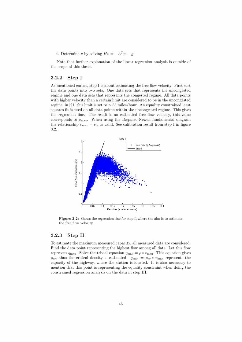
4. Determine v by solving Hv = −ATw − g.

Note that further explanation of the linear regression analysis is outside ofthe scope of this thesis.

3.2.2 Step I

As mentioned earlier, step I is about estimating the free flow velocity. First sortthe data points into two sets. One data sets that represents the uncongestedregime and one data sets that represents the congested regime. All data pointswith higher velocity than a certain limit are considered to be in the uncongestedregime, in [21] this limit is set to > 55 miles/hour. An equality constrained leastsquares fit is used on all data points within the uncongested regime. This givesthe regression line. The result is an estimated free flow velocity, this valuecorresponds to vmax. When using the Daganzo-Newell fundamental diagramthe relationship vmax = vcr is valid. See calibration result from step I in figure3.2.

Figure 3.2: Shows the regression line for step I, where the aim is to estimatethe free flow velocity.

3.2.3 Step II

To estimate the maximum measured capacity, all measured data are considered.Find the data point representing the highest flow among all data. Let this flowrepresent qmax. Solve the trivial equation qmax = ρ ∗ vmax. This equation givesρcr, thus the critical density is estimated. qmax = ρcr ∗ vmax represents thecapacity of the highway, where the station is located. It is also necessary tomention that this point is representing the equality constraint when doing theconstrained regression analysis on the data in step III.

45

Figure 3.3: This figure displays the line for the maximum flow. It alsodisplay the intersection between the regression line for free flow velocity andthe maximum flow.

3.2.4 Step III

Use all data points from the congested regime, the second set of data. Only datafrom the second set is considered during step III. The data from the second setis partitioned into bins of non overlapping data along the horizontal axis witha certain amount of data in each bin. Each bin contains a defined amount ofdata points, in [21] they choose a bin size of ten data points, for a graphicalexplanation see Figure 3.5.

To determine how to estimate if a data point is an outlier or not, the authorsof [21] chooses to make use of quartiles in statistical theory. See figure 3.4 fora graphical representation. Figure 3.4 also shows how the box plot relates toa Gaussian distribution. The theory for finding data points that lie withinthe box plot is used in the binning procedure. If the data point lie outsidea specified interval e.g. a value x > Q3 then it is considered as an outlier.Note that the use of quartiles does not require a Gaussian distribution [31] andthat a Gaussian distribution is not assumed later in the automatic empiricalcalibration procedure.

46

-4σ -2σ 0σ 2σ 4σ

50.00 % 24.65 %24.65 %

Q1 Q3

Q1 - 1.5 × IQR Q3 + 1.5 × IQR

1

Figure 3.4: This figure represents how the different quartiles relates to themass of probability.

Each bin is then summarized by BinDensity which is equal to the mean ofthe density values in the bin. After each horizontal bin value (BinDensity) hasbeen determined, then each bins vertical value (flux) is determined via (3.5) and(3.6). The result from (3.6) gives the largest non outlier with the highest flowand density value.

Bin = {f1, f2, . . . , fi} (3.5)

BinFlow = maxfi

(fj |fjε Bin, fi < Q3 + 1.5IQR) (3.6)

where i is the index of data point i in each BinDensity, j is the j : th bincomputed by (3.6) and Q3 is the 75th percentile of the data points in the binand IQR is the interquartile range.

1

Figure 3.5: This figure displays an example bin. The bin size is ten datapoints. The red point represents the mean density (it does not belong to theactual set and can threfore be placed anywhere in the bin). Black points areoutliers, sorted out using (3.6). The purple point refers to the chosen flow.The final value for the bin is the flow from the purple point and the densityfrom the red point.

The result from calculating (3.6) creates a BinDensity - BinFlow pair (Bin-Pair). When all bins have been calculated, a constrained least-square regressionmethod is then applied to the BinPairs, thus obtaining the last relationship of

47

the fundamental diagram representation. The constraint is given by the freeflow capacity. The result from the calibration is summarized in Table 3.3 andin figure 3.6.

Table 3.3: This table presents the calibration results from the example.Note that the parameters are estimated using aggregated data from PeMSstation ID 400309 from five lanes.

Parameter Value UnitFree-flow velocity 27.65 meter/secondBackwave speed 11.44 meter/secondMaximum density 0.3172 vehicles/meterFlow capacity 2.567 vehicles/secondDensity capacity 0.0928 vehicles/meter

Figure 3.6: Shows the resulting fundamental diagram from the calibrationprocess.

3.2.5 Remarks

Note that this calibration procedure assumes that the Daganzo-Newell funda-mental diagram is used. Due to this, the calibration method needs to be adaptedto a hyperbolic-linear fundamental diagram instead. The main reasoning behindthis is, when using the Daganzo-Newell fundamental digram it is assumed thatvcr = vmax, which is not the case when using a hyperbolic triangular diagram.How the algorithm is adopted to fit this kind of diagram will be explained in5.1.

3.3 Complex method

The Complex method, introduced by M.J. Box in 1965, is a non-gradient searchalgorithm for finding the optimum value for non-linear functions depending on

48

multiple decision variables [32]. The Complex method, or simply the algo-rithm considering its nature, assumes that the decision variables are enclosedwithin an admissible region or, in other words, that the target function is thesubject to at least one explicit constraint. All constraints are assumed to bein-equality constraints. The fact that the Complex method is a non-derivativesearch algorithm speaks in favour of many applications since the objective func-tion derivative would never need to be calculated. This would allow the user tochoose any objective function during the evaluation of the model performancewithout any changes to the implementation of the Complex method.

Several authors of different traffic modelling papers have used the Complexalgorithm for solving their parameter estimation problems in an orderly fashion,see for instance [23,27,28].

This section gives an introduction to the Complex method as it is describedin [32–34]. The initial presentation is general and later explained with an ex-ample of how to solve trivial optimization problem with the Complex method.The later part of this section concerns the application of the Complex methodfor parameter estimation in traffic models.

A disadvantage of the algorithm that should be noted is that a solutioncannot be proven to be a global optimum (the search effort might get stuck atlocal minimum or maximum) [33,34]. This issue is usually handled by runningthe algorithm several times with different initial conditions within the admissibleregion. It should also be noted that the algorithm demands that the targetfunction is evaluated many times, which could be costly from a computationalperspective. The user should therefore be careful when choosing the dataset tocalibrate against, there is probably no need to run a calibration process over along time period that only encompasses a single traffic state for example.

3.3.1 Formal presentation

For explanation of the Complex method, consider the following problem:

min f(x1, . . . , xN )

subject to xLi ≤ xi ≤ xUi , i = 1, . . . , N

xLi ≤ xi ≤ xUi , i = (N + 1), . . . , (N +M)

where the N constraints are explicit, while the M constraints are implicit, xLiis the lower limit and xUi is the upper limit for the variable xi.

The difference between explicit and implicit constraints is that explicit con-straints define a range for the decision variables xi, i = 1, . . . , N while implicitconstraints are either linear or non-linear functions of the decision variablesxi, i = 1, . . . , N [33]. In other words, the variables xi, i = (N+1), . . . , (N+M)are definitely functions of xi, i = 1, . . . , N while the lower bounds xLi andthe upper bounds xUi for i = (N + 1), . . . , (N + M) are either functions ofxi, i = 1, . . . , N or constants.

During the initialization of the Complex method is a so called complex gen-erated from the admissible region that is expressed by the explicit constraintswhile any violation of implicit constraints are handled retroactively [33]. Thecomplex is a collection of N -dimensional points and it is assumed that complex

49

has at least K > (N + 1), N -dimensional feasible points once it has been gen-erated. The point of choosing a complex with K > N + 1 points is to ensurethat the complex keeps its dimensionality when the points are moved around inthe N -dimensional space during the iterations of the Complex method. If thecomplex has to few members, it could collapse, or rather, flatten itself againstthe first constraint that is reached during the movement in the N -dimensionalspace [32].

The initial complex {xij}, i = 1, . . . , N, j = 1, . . . , K, where the subscripti indicates the variable and the subscript j indicates the complex member, isgenerated as follows. Assume that one feasible point is known (one that doesnot violate any of the implicit and explicit constraints). All other K − 1 pointsj are generated randomly as

xij = xLi + rij(xUi − xLi ), i = 1, . . . , N, j = 2, . . . ,K (3.7)

where rij is an uniformly distributed random variable expressed as rij ∼ U(0, 1).The reason for why a feasible point must be given is that (3.7) leaves no guar-antee of non-violated implicit constraints and a feasible point is needed in orderfor the Complex method to know in which direction an infeasible point shouldbe moved. Note however that there is no need for an initial point if no implicitconstraints are present, the entire initial complex can be generated with (3.7)in that case.

If an implicit constraint is unsatisfied by a generated point k during the ini-tialization of the complex method, that point is moved half the distance towardsthe centroid of the points generated thus far. This reveals the importance ofhaving an initial feasible point since if the first randomly generated point vi-olates an implicit constraint, it must be moved towards that point until it isfeasible. The centroid xiC along dimension i = 1, . . . , N is defined as

xiC =1

k − 1

k∑j=1

(xij), j 6= k (3.8)

where k is the index of the last point that was generated and thus the size of thegenerated complex {xij} thus far along dimension j, including the point thatviolated the constraint. A new complex point is generated according to

xNik =xiC − xOik

2, i = 1, . . . , N (3.9)

where the superscript N denotes a new point, O denotes the old point thatviolated any constraint and xNik is the value of the ith coordinate of the newcomplex point. This procedure leads to a feasible point, if the feasible region isassumed to be convex, since it can be repeated until all constraints are satisfied.

The points of the complex are randomly scattered over the feasible regiononce the complex of feasible points is generated. The value of the target functionis then evaluated for every single point and it is noted which of the complexmembers that have the best and worst value. Those two points are used tochecked the imposed convergence criteria

fmax − fmin < β (3.10)

Reference [33] notes that (10−3 − 10−4)fmax is a common value of β.

50

The worst point generated, called xW , is rejected if (3.10) is a false state-ment. If the problem is a minimization problem, the worst point is of course theone with the greatest function value. In this case, rejecting the point means thatit is moved towards the centroid of the remaining complex members, creating anew point xNew according to (3.11).

xNewik = α(xiC − xWik ) + xiC , i = 1, . . . , N (3.11)

where the expression for the centroid xiC is similar to that expressed by (3.8).As for the value of the reflection parameter, or step length, α in (3.11), [32]found that an α = 1.3 should be a suitable choice.

The new point xNewik is evaluated to see if it satisfies the explicit constraints.If it is not, it is moved a small distance δ within the limit of the constraintthat is violated (and then rechecked again). Reference [32] states that 10−6 hasproven to be a functional value of δ and also that the chance of the correctedpoint to be within the subspace of the other points should be fairly small.

If any implicit constraint is unfulfilled after the reflection of the worst point,the trial point should be moved halfway towards the centroid of the better pointsjust as during the generation of the initial complex and according to (3.9), butthen with K − 1 in the denominator.

In the original formulation of the complex method the progress stated by(3.10) - (3.11) is repeated until the entire complex (the set of points) has movedto the centroid. At that time the convergence criteria expressed by (3.10) shouldbe fulfilled. In other words, the algorithm stops when the complex (the points)has collapsed to a singular location in the parameter space, in which case thetarget values are nearly the same for each individual point of the complex.

It has been noted that the Complex method can get stuck around a localoptimum if that local optimum happened to be the centroid [34]. By repeat-ing the movement for the worst member4 is a way to overcome this issue. Atrial point can be expressed by a gradual movement of the point towards theminimum value as long as the trial point continues to be the worst one of thecomplex. It is a risk though that this might result in that a trial member istoo near another point which could risk a collapse of the complex. This risk ofa collapse can be handled by the introduction of a new random value that isadded to the trial point. Also, this random search increases the search effortin relation to the simple reflection. This modification (or extension since thisnew movement is introduced only if a trial point is a repeater) of the Complexmethod can be expressed by (3.12).

xN(new)ik =

xN(old)ik + εxiC + (1− ε)xBik

2+ (xiC − xBik)(1− ε)(2R− 1) (3.12)

where xBik is the best point of the complex, R is a uniformly distributed randomnumber, R ∼ U(0, 1) and ε is defined by (3.13).

ε =( nrnr + kr − 1

)(nr+kr−1nr

)(3.13)

where kr is the number of times that xNik in (3.12) has been the worst point(a repeater), nr is a constant. A nr = 4 could be an adequate choice for that

4The repeated point is called a trial point prior to that, if it is not longer the worst one.

51

constant. Note that the previous worst point xN(old)ik in (3.12) is always updated

to be the previous trial point.A flow chart for Complex method can be found in [33, p. 119]. That model

was followed when Figure 3.7 was created, this figure shows the overall processof the Complex method if one chooses to utilize the half distance movementtowards the centroid and if there are implicit constraints present.

52

Start

Select one feasiblestarting point.

Generate the initialcomplex of K points.

Are the explicitconstraints violated?

Move the point adistance δ within theviolated constraint.

Are the implicitconstraints violated?

Is the initial com-plex generated?

Evaluate the objectivefunction at each point.

Run model for everycomplex member.

Check conver-gence criteria.

Stop.

Replace the worstpoint by a reflectionthrough the centroid.

Is the new point stillthe worst point?

Move the pointhalf its distance

towards the centroid.

not ok

ok

ok

ok

not ok

yes

yes

no

no

not ok

Figure 3.7: Complex method (algorithm) presented ad a flow-chart forsolving in-equality constrained optimization problems.

53

3.3.2 Example: Visualization of the complex movement

In this section, an example of the Complex algorithm application is presented.The goal is to find optimum solution to the following minimization problem:

min f(x1, x2) = x21 + x22

subject to −5 ≤ xi ≤ 5, i = 1, 2

The target function f(x1, x2) is one with a global minima within the admissibledomain at (x1, x2) = (0, 0) for which f(x1, x2) = 0. In the figure below it ispossible to follow the movement of the complex members as they end up in thecomplex centroid near the optima.

x1

x2

−5 0 5−5

0

5

x1

x2

−5 0 5−5

0

5

Figure 3.8: An example of how the complex moves towards the optimawith the first movement on the left and the complete movement on theright. The red cross marks the current centroid. The leftmost figure depictsa movement where the complex method tries to move a point outside theboundaries.

3.3.3 Example: Calibration of a single edge highway model

This section should be seen as a bridge between a highway model and theComplex model. The target of highway model calibration is to decrease thedifference between model output, predicted state and field observations. Thisdifference is expressed by a function that often returns a single scalar value. Inthis section the traffic model will be described as dynamic state vector equationsso that the parameter estimation problem is well posed.

Recall the cell transmission model for velocity (CTM-v). The CTM-v ex-pressed that the velocity field on the highway evolves in time according to certainrules expressed by the transformed Godunov velocity flux functions. With theambition to calibrate by comparing model output define three vectors:

vT = [v0, v1, . . . , vimax] (3.14)

uT = [v−1, vimax+1] (3.15)

54

yT = [v,x] (3.16)

Where v state vector holding the velocity for each cell i ∈ {0 . . . imax}, u isan input vector holding the conditions to be imposed at the boundaries and yis an output vector holding the state at the measurement point as well as the(current) parameter set x that led to that output.

The state vector v represents the velocity field over a single edge (for whichone fundamental diagram is used). The edge consist of imax + 1 cells.

The input vector u holds measurements from the boundaries that will sub-stitute references to what was referred to as ghost points earlier, i.e. they do notlie in the physical domain but provide the boundary conditions to be imposedon the modelled highway.

The output vector y can in general be any traffic state variable. It is impor-tant to note which kind of data source the model output should be comparedwith. If the user wants to use stationary speed detectors then the velocity fieldfrom the model output may have to be transformed from space mean speed totime mean speed (since the detector only measures speed at a single point inspace).

The model is characterized by a vector of unknown parameters x = (ω, vmax,ρmax) (e.g. the free flow speed). This vector is the estimation subject and istreated as a variable during the parameter estimation procedure.

Assuming that the velocity field evolves according to the CTM-v, which nowis label with F (and not the standard update algorithm label M since only asingle edge is considered in this explanation), can a non-linear dynamic statevector equation be expressed according to

v(n+ 1) = F [v(n),u(n),x] (3.17)

The output vector is defined by

y(n) = T [v(n),x] (3.18)

where T is an operator that transforms the values in the output vector v tothe domain in which the field measurements lie in (e.g. T represents a processwhere a single cell is extrapolated). The objective is to find the parameter set xthat minimizes the deviation between model output and the field observationsy. As a short proof of concept the Complex method is now to be used forparameter estimation of a small CTM-v model.

Consider Figure 3.9, it depicts sensor arrays (detectors) on the highway E4near Kista, Sweden. The test site stretches from detector 68,330 to detector66,710 and traffic travels in that direction. In between these two detectors liesdetector 67,400. All of these detectors captures the velocity on the highwayover time. This stretch of highway spans over 1.7 km and is divided into 17 cellsi ∈ {0 . . . 16}, each being 100 meters long (∆x = 100m).

55

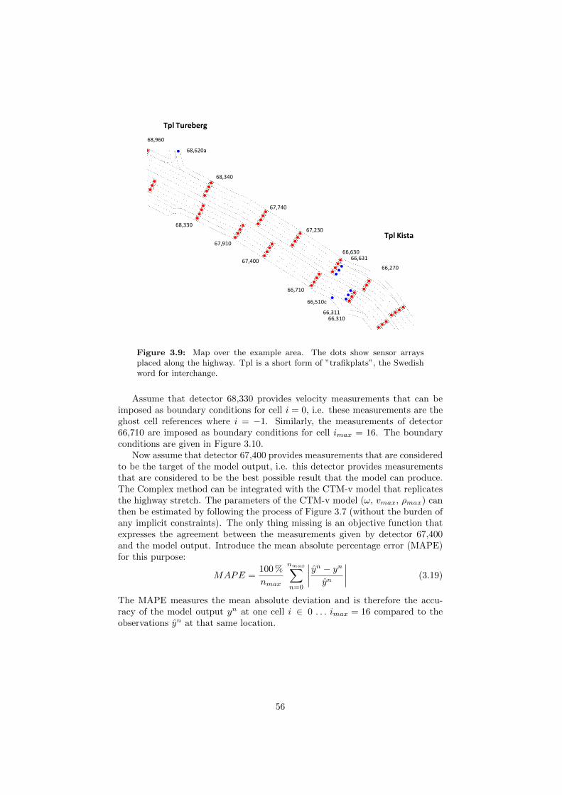
Endast Körfältsdetektor

Körfältssignal och Körfältsdetektor

Endast Körfältssignal

MCS VSTÖversikt KFS/KFD

Tpl Hagbylund

3,315

3,315

3,305

3,640

3,530

3,745

4,045

4,215

4,465

4,875

5,155

4,165

3,950

4,465

4,875

Häggvikstunneln

1,740

2,000

2,240/2,240c

2,320

2,650

2,970

3,115

2,775

2,440Törnskogstunneln

72,890

1,390

1,160

0,9701,130

1,300

1,590

0,830

Tpl Häggvik

1,590

1,450

1,800/1,800a

1,985

Tpl Tunberget

70,830

71,200

71,310g

71,550e

0,820

71,660

72,010

72,330

71,440

0,5700,970

71,400

0,450

70,960

0,200

66,270

67,230

Tpl Tureberg

Tpl Kista

66,630

67,740

68,340

68,620a

68,960

69,430

69,690

69,990

70,52070,560

70,070

69,820

69,390

69,130c

68,800

68,330

67,910

67,400 66,631

Tpl Järva Krog

Tpl Sörentorp

63,580

63,040

65,000

64,650

64,090

64,650

65,420

64,970

64,090

63,580

62,645

63,040

62,070

62,410/62,410m

63,215

65,420

66,310

65,815

65,815

66,710

66,510c

66,311

Tpl Tomteboda

57,140 57,820

57,275

59,835

59,740

60,265

58,590c 58,610c

57,435

60,060

59,420

Tpl Frösunda

Tpl Haga Norra

61,270

61,605

62,070

62,220

61,860

60,645

61,395

61,000

60,990

61,115c

60,490

Tpl Fredhäll

Tpl Lindhagensgatan

Tpl Karlberg

Fredhällstunneln

58,865d57,140 57,820

58,140

55,400

55,210

54,880

55,620

56,160

56,490

56,780

57,055

55,97555,975c

56,160c

55,505

55,650

57,690

58,01058,205

57,690a

57,430

58,555 58,570

58,555b 58,570b

58,59058,590c 58,610c

58,610

55,885

55,165

56,575

56,780

57,010

57,32057,165

55,330

55,185

Tpl Stora Essingen

54,145

Tpl Lilla Essingen

53,870

53,590

52,535

53,120

53,595

53,115

52,745

52,220

52,720

Tpl Gröndal

Tpl Nyboda52,535

51,890 / 51,890h

0,310

0,005 / 51,895

51,0400,535

0,455u0,235u

51,630

51,670

51,425

52,21552,030

51,680h 51,530h

55,03054,630

54,295

54,420

54,225

54,630

53,955

2009-06-29 / Stefan Christensson/ Inmind Scandinavia AB

Tpl Västberga

Tpl Västertorp

Tpl Bredäng

50,225n / 50,225

50,660

49,710

49,530

48,935 49,220

48,38547,98047,63547,255

47,46548,29047,800

48,935

48,620

49,370

50,165

50,395

50,570

50,890

0,535

0,565u

0,905u / 0,905

51,370

0,750

0,900

1,075

51,610e

51,430e

49,770 / 49,770m

51,085e 51,085

46,895

49,970m

1,435

1,170a / 1,170

1,270

Tpl Mossen

10,950

10,950

11,210

11,440

11,675

11,830

12,080

11,830

11,675

11,440

11,210

12,330

12,575

12,770

12,935

13,14012,770

12,935

13,140

12,030

12,270

12,520

Tpl Täby Kyrkby

Löttingetunneln

Tpl Haga Södra

Tpl Linvävartorpet

59,980

59,335

59,440

59,530

59,530

59,425

60,490

58,865d58,865

59,125

58,940

Eugeniatunneln

58,685

58,57058,570b

59,260

59,33559,360

59,25559,155

5,165

7,5804,805

5,440 5,730 6,000

6,440

Tpl Nacka

Tpl Lugnet7,2807,075

6,880c

6,880

6,880

6,825

6,765

6,735

6,8206,690

6,615

6,680

6,595

6,540

6,415

6,365

6,260

6,180

6,380

6,500

6,295

6,0256,115

6,025

5,945 / 5,945a

2,0852,2402,300e

2,390e

2,480e

2,625e

2,750e

2,500

2,170

23,925

23,825

2,315 2,515

23,620

2,600

2,870h

2,740 2,840

3,015h

2,765

2,97523,865r

23,575r

23,495r

2,695h

2,595h

2,370h

5,055b

23,490

2,970

Tpl Nyboda

Södra Länken23,325

23,22023,130

22,915

3,105

3,215

3,3753,335a

3,430a

3,2703,155

3,460d

3,360

3,600d3,705d

3,895d3,970d

3,980a

23,11523,205

23,285

23,375

23,050

22,800

22,500

3,510

3,680a

3,505

4,810

4,630

4,5104,395

53,135e4,275

53,030e

52,950e

52,875e

52,755g52,685g

52,550g

52,460e

52,335e

52,230e

52,155g

52,050

52,335g

52,460g

3,210u

3,515u

3,320

3,515s

3,710u

3,880u

4,230r

52,970g

52,875g

4,1804,270u

4,370u

4,470u

3,71053,400g

3,93553,270g

53,155g

3,705

3,870r3,985r

4,095r

3,880

4,130

4,070u

3,985u

5,3155,415b

5,145b

4,610u

4,795

4,970

5,155d

4,9854,990a

5,090a

5,180

5,195a

5,190

4,455

4,370

4,605

Tpl Åby0,905u / 0,905

1,585b1,585

Södra Länken

1,270

1,8851,960

1,6701,670c1,505

1,550c

1,660

1,960

1,845

51,88051,645

51,405

Figure 3.9: Map over the example area. The dots show sensor arraysplaced along the highway. Tpl is a short form of ”trafikplats”, the Swedishword for interchange.

Assume that detector 68,330 provides velocity measurements that can beimposed as boundary conditions for cell i = 0, i.e. these measurements are theghost cell references where i = −1. Similarly, the measurements of detector66,710 are imposed as boundary conditions for cell imax = 16. The boundaryconditions are given in Figure 3.10.

Now assume that detector 67,400 provides measurements that are consideredto be the target of the model output, i.e. this detector provides measurementsthat are considered to be the best possible result that the model can produce.The Complex method can be integrated with the CTM-v model that replicatesthe highway stretch. The parameters of the CTM-v model (ω, vmax, ρmax) canthen be estimated by following the process of Figure 3.7 (without the burden ofany implicit constraints). The only thing missing is an objective function thatexpresses the agreement between the measurements given by detector 67,400and the model output. Introduce the mean absolute percentage error (MAPE)for this purpose:

MAPE =100 %

nmax

nmax∑n=0

∣∣∣∣ yn − ynyn

∣∣∣∣ (3.19)

The MAPE measures the mean absolute deviation and is therefore the accu-racy of the model output yn at one cell i ∈ 0 . . . imax = 16 compared to theobservations yn at that same location.

56

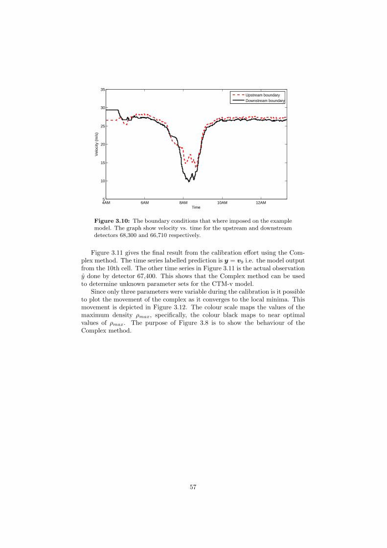
4AM 6AM 8AM 10AM 12AM5

10

15

20

25

30

35

Time

Vel

ocity

(m

/s)

Upstream boundaryDownstream boundary

Figure 3.10: The boundary conditions that where imposed on the examplemodel. The graph show velocity vs. time for the upstream and downstreamdetectors 68,300 and 66,710 respectively.

Figure 3.11 gives the final result from the calibration effort using the Com-plex method. The time series labelled prediction is y = v9 i.e. the model outputfrom the 10th cell. The other time series in Figure 3.11 is the actual observationy done by detector 67,400. This shows that the Complex method can be usedto determine unknown parameter sets for the CTM-v model.

Since only three parameters were variable during the calibration is it possibleto plot the movement of the complex as it converges to the local minima. Thismovement is depicted in Figure 3.12. The colour scale maps the values of themaximum density ρmax, specifically, the colour black maps to near optimalvalues of ρmax. The purpose of Figure 3.8 is to show the behaviour of theComplex method.

57

4AM 6AM 8AM 10AM 12AM5

10

15

20

25

30

35

Time

Vel

ocity

(m

/s)

PredictionObservationMAPE = 4.8 %

Figure 3.11: Model output after calibration in dashed green versus ob-served velocities. The mean absolute percent error was 4.8 % after calibra-tion.

This concludes the presentation of the Complex method for parameter esti-mation. The Complex method, a non-gradient search algorithm was presented.That it is of the non-gradient type speaks in favour of its use since M, theupdate algorithm of the CTM-v presented earlier, is not differentiable. On topof that the ensemble Kalman filter is wrapped around the M for the purposeof data assimilation. A black-box algorithm, such as the Complex method,is therefore attractive. The actual implementation of the Complex method ispresented in a later chapter.

58

46

810

1214

25

26

27

28

29

300.08

0.09

0.1

0.11

0.12

0.13

0.14

ω (m/s)vmax (m/s)

ρ max

(m

−1 la

ne−

1 )

0.085

0.09

0.095

0.1

0.105

0.11

0.115

0.12

0.125

0.13

0.135

Figure 3.12: The movement (all iterations) of the complex during the cali-bration of the example model. Each complex point is given in the coordinates(ω, vmax, ρmax).

59

Chapter 4

System Description

This chapter is mainly an outcome from the system analysis that were conductedand the purpose of introducing this chapter, is to provide an overview of therelevant parts of the Mobile Millennium system for the reader. It also servesthe purpose of mapping the different parts of the system that are used in thecalibration framework that this report is presenting. It will also present a listof all parameters that the framework will try to estimate and calibrate.

4.1 Overview

The system mainly consists of three parts; measurement loader, highway modeland the ensemble Kalman filter. All of these three parts have hard coded, ad-hoc calibrated parameters. Figure 4.1 shows how the data flows throughoutthe system. Data is loaded from a database where data sources can be of typeprobe or stationary data. All data that is loaded is pre filtered. The user canchoose to use data from no data source, a specific data source, some specificdata sources or all data sources. The highway model utilize the CTM-v modeltogether with the velocity from the current time step to predict the velocity fieldfor the next time step. The default time step is six seconds. The third part isthe ensemble Kalman filter; it fuses the predicted data with the measured data.All parameters found in the system when conducting the system analysis arelisted in the Appendix A. As mentioned earlier in this section, all parameterslisted in this section are all static and hard coded. This makes it impossible tocalibrate them in an automatic matter. Therefore system modifications werenecessary. The modifications made will be explained later in the thesis.

60

PeMS feed Filter

Probe 1 feed Filter

Probe 2 feed Filter

EnKF (Filter)

Solve links

Solve junctions

Measurement input

Highway model

1

Figure 4.1: This figure shows the data flow for the Mobile Millenniumsystem. The measurement loader loads data from the database with storeddata and feeds it to the highway model predicts and fuses the data using theensemble Kalman filter.

4.2 Measurement loader

The main purpose of the measurement loader is to enable the user to chooseand load any data from any source available in the database. There are hardcoded parameters with significance to the system in the measurement loader.More about why it is significant is mentioned in after Table 4.1. Therefore thispart of the highway model is relevant for this thesis. The relevant parametersfor measurement loader is summarized in Table 4.1.

Table 4.1: This table displays all parameters connected to measurementloader that is relevant for the thesis. Note that the parameters in this tableare for one lane.

Parameter Current Value UnitFree-flow velocity 27.0 meter/secondCritical velocity 25.0 meter/secondBackwave speed 5.36 meter/secondMaximum density 0.124 vehicles/meterFlow capacity 0.667 vehicles/secondDensity capacity 0.0247 vehicles/meter

The data where v > vcr1 is too noisy for the ensemble Kalman filter when

1These measurements are considered to exist in the uncongested regime

61

using stationary sensors. Therefore, a fit of the data in the uncongested region istherefore made using the fundamental diagram. The flow gets mapped accord-ing to the fundamental diagram and transformed to velocity2. Therefore thefundamental diagram parameters for each link is connected to the measurementloader.

4.3 Highway model

The highway model predicts the traffic state for the next time step. The inputinto highway model is the current state for the current time step. Parametersconnected to highway model is displayed in Table 4.2.

Table 4.2: This table displays all parameters connected to the highwaymodel that is relevant for the thesis. All parameters connected to the fun-damental diagram is based on lane.

Parameter Current Value UnitSplit ratio defined for each junction percentageSinks 5*max capacity vehiclesSources 0.6*max capacity meter/secondFree-flow velocity 27.0 meter/secondBackwave speed 5.36 meter/secondMaximum density 0.124 vehicles/meterFlow capacity 0.667 vehicles/hourDensity capacity 0.0247 vehicles/meter

Note that measurement loader and the highway model have common pa-rameters. This is due to certain properties in the system. The system is madefor using the ensemble Kalman filter, which is not stable when having to noisymeasurements. This means when measurements are considered to be in uncon-gested regime3 from stationary sensors is tampered with, since the ensembleKalman filter cannot cope with noisy data.

4.4 Ensemble Kalman filter revisited

The ensemble Kalman filter is responsible for fusing the predicted state with themeasured state. In Table 4.3 all relevant parameters for the ensemble Kalmanfilter are summarized.

2This is only true if the measurement loaded lies within the density domain3The measurements in uncongested regime are generally too noisy for the ensemble Kalman

filter.

62

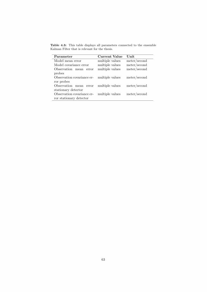
Table 4.3: This table displays all parameters connected to the ensembleKalman Filter that is relevant for the thesis.

Parameter Current Value UnitModel mean error multiple values meter/secondModel covariance error multiple values meter/secondObservation mean errorprobes

multiple values meter/second

Observation covariance er-ror probes


Observation mean errorstationary detector


Observation covariance er-ror stationary detector


63

Chapter 5

Implementation ofCalibration Procedures

This chapter will present how the authors implemented the calibration proce-dures and the framework. The first section, section 5.1 will focus on the im-plementation of the automatic empirical calibration method. The next section,section 5.2, will focus on how to assign parameters connected to the fundamen-tal diagram to links. The last section of this chapter, section 5.3, presents howthe complex method have been adapted, implemented and integrated into thesystem.

5.1 Implementation of the automatic empiricalcalibration method

As mentioned in 4.3, due to the fundamental diagram that is used in the system,see (2.20), it is not possible to apply the calibration method without modifica-tions. This section will present three adapted versions of the modified calibrationmethod. Note that later on, the unmodified calibration method is referred toas the original, the modified calibration methods are referred to as versions.

The method is going to calibrate the parameters; ρmax, ρcr, vcr, vmax, wf ,and qmax, the parameters for the Hyperbolic-Linear diagram for each stationarysensor in the system. The example from the section 3.2, is used as an examplein this section as well.

5.1.1 Version I

This version utilize somewhat the same approach as the original method. How-ever, the order in which the parameters are estimated as well as the methods forestimating them are changed. Instead of finding vmax first, this version focus onfinding the capacity first, which is expressed by vcr ∗ρcr = qmax. After that, thesecond step is to find the back wave propagating speed wf and the maximumdensity ρmax. The last step is to estimate the free flow velocity vmax and to dothis, the continuity constraint (2.21) is used. A step by step description of themethod is as follows.

64

Step I

Find the maximum capacity by searching through all data points. Searchthrough the measured data points, find the data point with highest flow mea-sured. Let that data point with the highest measured flow and density representthe capacity. Alas vcr, ρcr and ρmax estimated. The graphical result from stepI is presented in 5.1.

Figure 5.1: Shows the maximum capacity found.

Step II

The back wave propagating speed wf as well as the maximum density ρmax isestimated through the same binning method as in the original, for the exactmethod see 3.2.4. The graphical result from step II is presented in 5.2.

65

Figure 5.2: Shows the result from the binning process and regression anal-ysis in step II.

Step III

This step involves finding the last parameter vmax using the continuity con-straint. Since ρc, rhomax, wf already have been estimated, the continuity con-straint (2.21) from 2.1.4 can be used to estimate vmax. The graphical result canbe viewed in figure 5.3. All calibrated parameters for version I can be found in5.1.

Figure 5.3: This figure shows the calibration result from step III version I.

66

Table 5.1: Calibration results for the example in section 3.2. Note that theparameters are estimated using aggregated data from five lanes.


5.1.2 Version II

This version is using the same approach as version I, the main difference is howthe capacity is estimated. Instead of using the intersection between the free flowvelocity and the data point with the highest flow measured, this version insteadapplies the binning concept to the data points with the highest flow measured.The result from this binning is used to find the capacity of the road. To estimatethe back wave propagating speed and density max, the same approach as theoriginal is used. The last step is to estimate the free flow velocity and to dothis, the continuity constraint is used in this version as well.

Step I

Just as version I, this step involves finding the maximum capacity. Instead ofusing the data point with the highest flow, bin the data points with the highestflows instead. The characteristics of data, where the flow is near its maximum,makes it reasonable to bin the tip in the following way. Sort all data point byflow. Choose a bin size N . Binning of the tip is motivated by the fact that thedata point, even though filtered, are not trust worthy. Note that the filtering ismore strict in this version of the binning method. The binning is made using(5.1)-(5.3).

Bin = {f1, f2, . . . , fn} (5.1)

Start to estimate the density of the bin, by using (??) and (5.1).

BinDensity = maxfi

(fj |fjε Bin, fi < Q3) (5.2)

Start to estimate the density of the bin, by using the bin from (5.1) and(5.3).

BinFlow = minfi

(fj |fjε Bin, fi > Q1) (5.3)

The result from the binning method of the tip is an estimate of the maximumcapacity of the highway. Alas the ρc, vc and qmax.

67

Figure 5.4: This figure depicts the results from step I, when trying tocalibrate the parameters for the fundamental diagram using version II.

Step II

The back wave propagating speed wf as well as the maximum density ρmax isestimated through the same binning method as in the original, see 3.2.4.

Figure 5.5: This figure depicts the results from step II, when trying tocalibrate the parameters for the fundamental diagram using version II.

Step III

Use the continuity constraint to estimate vmax exactly in the same way as de-scribed in Version I step III. The graphical solution is visualized in figure 5.6

68

Figure 5.6: This figure shows the final results from using version II.

Table 5.2: This table presents the calibration results for the example insection 3.2.


5.1.3 Version III

Step I, step II and step III is identical to the original automatic empirical cali-bration method except that it have been extended with one step. The last stepin this version , the same method for estimating vmax as version I and versionII.

Step I

Just as the original method, see 3.2.2, find an initial value of vmax, using a linearregression on all data points below a certain density to find vmax. For graphicalrepresentation see figure 3.2. For more detailed information see section 3.2.2.

Step II

To find the maximum capacity (vc, ρc and qmax), find the largest flow. Just asstep I, step II is a direct copy of step II from the original method, see 3.2.3.Use the intersection between this line and the regression line from vmax. Forgraphical representation see figure 3.3.

69

Step III

The back wave propagating speed wf as well as the maximum density ρmax,is estimated through the same binning method and constrained least squareregression analysis as in the original method, see 3.2.4.

Step IV

This step involves finding the last parameter vmax using the continuity con-straint, see 5.1.1. The graphical result is presented in 5.7 and the estimatedparameters is summarized in Table 5.3.

Figure 5.7: This figure depicts the results from step IV, when trying tocalibrate the parameters for the fundamental diagram using version IV

Table 5.3: This table presents the calibration results for the example insection 3.2 using version III.


5.1.4 Implementation remarks

The fundamental diagram calibration procedures was implemented into the sys-tem as an independent module. In general this means that the parameters canbe calibrated without any interaction with the highway model. The calibrationprocedure loads filtered data from a PeMS with a certain time aggregation fora defined time interval, the default setting for the aggregation period is 30 sec-ond long. The outcome of the measurement during the aggregation is the mean

70

traffic state for the aggregated time period on the point on the highway wherethe PeMS station placed. The measured data point consists of three measure-ments, the velocity, the flow and the density, where the velocity measured isthe mean velocity over the 30 second period; the flow is equal to the mean flow;the density is the mean density. After all data have been loaded by project, thefundamental diagram calibration procedure stars. When all parameters havebeen estimated, they are inserted into the database and keyed by the sensorsID. This enables the system to allocate a fundamental diagram to each linkspecifically. Since the calibration method is automated and the data from thePeMS stations are not trustworthy, even though the data is filtered, a qualitymetric was introduced. This quality metric estimates the ratio of data pointsbetween the congested regime and the uncongested regime, data availability andif the parameters are within reasonable bounds.

5.2 Link assignment

It is a requirement that each link should have an individual fundamental di-agram. To assign the fundamental diagrams to specific links, two differentmethods were developed. This section will present the two methods for assign-ing the fundamental diagrams. The two methods are similar to each other, themain difference between them, is how the fundamental diagram assignment ismade relative to which direction the traffic is streaming. The methods consistsof three steps each. Figure 5.8 shows the three steps graphically. Step I andstep II is identical for both of the methods. A link is defined as kn,j where n isthe order, n = 1, ..., N and j is the assigned fundamental diagram. Note thatthe notations for links are specific for this section only.

Step I

Define a list of links that is going to be assigned a flux function. The list needsto be sorted according to position and traffic direction, {k1,j , ..., kn,j} = K.

Example: Consider a small stretch of road represented by five links k1,j ,k2,j , k3,j , k4,j and k5,j . The links are positioned geographically in the followingorder, first k1,j , second k2,j and third k3,j . The traffic travels from link k1,j tok5,j . They can be considered sorted according to position and direction onlyand only if, {k1,j , k2,j , k3,j , k4,j , k5,j} = K where K is the list of the ordered setof links. See figure 5.8 I for graphical representation for step I.

Step II

Go through each link in the network. For each kn,j do: if there are no sensorconnected to the current link, do nothing. If there are one sensor connectedto the current link, assign the fundamental diagram j related to the sensor tothe link kn,j . Example: Go through each link, if there exist a sensor on thelink, assign the fundamental diagram from that sensor to the link. If there aremore than one sensor connected to the current link. Assign the fundamentaldiagram with the highest capacity to the link. Since the placement of thesensor on the link relative to the on and off ramps is not known, this is a wayfor avoiding ghost bottlenecks introduced by low capacity. The result from step

71

II is {k1,1, k2,1, k3,2, k4,2, k5,2} = K. See the graphical result for step II in figure5.8 II.

The method requires that there is at least one sensor connected to a link inthe network. It is also required that there is an existing fundamental diagramrelated to the sensor.

I. II. III.

1

Figure 5.8: This figure displays a graphical example for each step for thelink assignment. Circles is junctions, red squares is calibrated PeMS stationsyet to be assigned to a link, black lines are links. The arrow displays thetraffic direction. Links and PeMS stations with other colours are assigned afundamental diagram.

72

5.2.1 Forward link assignment

The forward link assignment assumes that the capacity and other road proper-ties propagates in the same direction as the traffic stream.

Step III

Find the first link km,1 with an assigned fundamental diagram in the network,set j = jcurrent. Assign the fundamental diagram from km,1 where links withn < m, this means to all upstream links. Then go through each link with n > m(all downstream links from n). If there is a sensor on link n with a fundamentaldiagram assigned then set jcurrent = j + 1. If there is no sensor on the link,assign current fundamental diagram j to that link.

Example I: Since step I and step II already have been made, we have{k1,j , k2,1, k3,j , k4,2, k5,j} = K. Find the first assigned link, that is k2,1,setj = jcurrent. Then assign all upstream links. The result becomes k1,1. Afterthat, assign all downstream links. No sensor found on k3,j , alas k3,j = k3,1.Go to next link. A fundamental diagram have been assigned to k4,2, update j,j = 1 + 1. Go to next link. No fundamental diagram assigned to this link, alasthe last link is assigned according to k5,2. For graphical representation of stepIII see 5.8 III.

5.2.2 Backward link assignment

The backward link assignment method assumes that the fundamental diagramcan be inherited upstream instead of downstream.

Step III

The same approach is used for backward link assignment method as for theforward link assignment method. First reverse the sorted set of links, so thatthe sorted list becomes the following {kn,j , ..., k1,j} = K. Since the methodspropagates upstream, update j according to j = j − 1 Then use the exact sameprocedure as step III to assign the links.

Example: Step I and step II are finished, we have that {k1,j ,k2,1,k3,j ,k4,2,k5,j}= K. Reverse the order {k5,j , k4,2, k3,j , k2,1, k1,j} = K, then find the first linkwith an assigned fundamental diagram, set j = jcurrent, in this example j = 2.After that, assign the fundamental diagram to all links downstream, the resultbecomes k5,2 and k5,1. After that begin assign fundamental diagrams to linksupstream. The next link k3,j will be k3,2. Go to next link k4,1, which have afundamental diagram, therefore update according to j = j−1. Go through restof the links. The final result from step III is {k1,1, k2,1, k3,2, k4,2, k5,2} = K. Forthe graphical representation see figure 5.8.

5.3 Complex method implementation

This part of the thesis describes the implementation of the complex method. Thepurpose with the upcoming sections is to visualize exactly what is happening inthe calibration process, but with figures and words rather than formulas.

73

The first section is a presentation of what is referred to as ground truthfollowed by a section on the conceptual thought behind the implementation inorder to increase the reader’s awareness of the calibration process. Then themajor data flow is presented to show how the different system parts interact.This system description is similar to the one initially made to the Mobile Mil-lennium system, see figure 4.1. The major difference is the introduction of afeedback loop and an increased system boundary where an extra data source isintroduced, which is used as the best possible estimate during the calibration.This section also presents simplifications made to the complex method prior toits implementation.

5.3.1 Ground truth

It has already been argued that a traffic model needs to be calibrated againstsome sets of field data, a ground truth that is treated as something like an idealmodel result. The ground truth can be observations at single points in space,such as traffic flow or time mean speeds, they can also be vehicle trajectoriesgiven by traffic probes that are constantly recording their location over timeor space mean speeds computed from travel time estimates. For this thesisBluetooth readings from the highway were available. From such readings traveltimes on the highway as well as space mean speeds can be computed. Thissection touches on the subject of space mean speed estimation from Bluetoothreadings.

In the first quarter of 2012 a set of Bluetooth detectors was placed along twodifferent experimental sites (the highways that where modelled) during approx-imately two weeks for each site. These sites are commonly referred to as I-880and I-15 Ontario. Bluetooth detectors of this kind have the ability to scan theBluetooth frequency band for any transmissions and capture the MAC-address1

of the unit that is transmitting as well as the time for that transmission.Simplified, the data collection procedure can be said to work as follows.

A Bluetooth detector is located at the beginning of a highway segment. Itdetects a passing transmitting Bluetooth unit at time t1 = 0 by identifying andstoring2 that unit’s MAC-address, see Figure 5.9. If the same MAC-addressis detected later on by another detector downstream of the first detector, andin a reasonable amount of time, say at t2 = 10 s the travel time between thosedetectors is t2−t1 = 10 s. Since the exact locations are known for both detectorsthe space mean speed of the Bluetooth device can be computed.

This detection process is repeated between each Bluetooth detector pairalong the highway and for many different unique transmitters (vehicles) thatare travelling on the highway. The travel time can then be computed as anaverage over a time period since many different transmitters are detected. Theuncertainty in travel time can then be expressed as a variance computed aroundthe sample mean. For this deployment the Bluetooth readings were aggregatedover 1, 5 and 15-minute intervals.

The final outcome from this procedure (collecting, filtering, aggregating,transforming) is the space mean speed for different time intervals along the

1A Media Access Control address (or MAC-address) is an unique label that identifies thenetwork interface of the unit in question.

2All Bluetooth reading are uploaded to a database for filtering and travel time computa-tions.

74

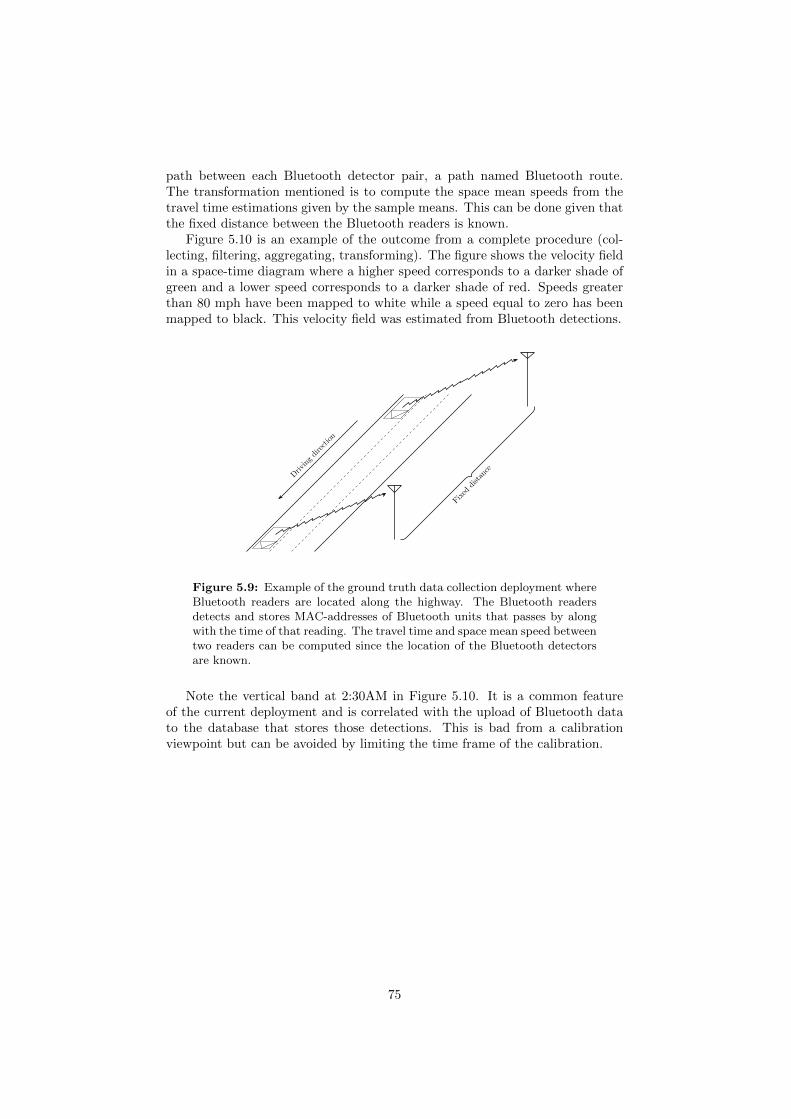
path between each Bluetooth detector pair, a path named Bluetooth route.The transformation mentioned is to compute the space mean speeds from thetravel time estimations given by the sample means. This can be done given thatthe fixed distance between the Bluetooth readers is known.

Figure 5.10 is an example of the outcome from a complete procedure (col-lecting, filtering, aggregating, transforming). The figure shows the velocity fieldin a space-time diagram where a higher speed corresponds to a darker shade ofgreen and a lower speed corresponds to a darker shade of red. Speeds greaterthan 80 mph have been mapped to white while a speed equal to zero has beenmapped to black. This velocity field was estimated from Bluetooth detections.

Drivingdirection

Fixeddistance

1

Figure 5.9: Example of the ground truth data collection deployment whereBluetooth readers are located along the highway. The Bluetooth readersdetects and stores MAC-addresses of Bluetooth units that passes by alongwith the time of that reading. The travel time and space mean speed betweentwo readers can be computed since the location of the Bluetooth detectorsare known.

Note the vertical band at 2:30AM in Figure 5.10. It is a common featureof the current deployment and is correlated with the upload of Bluetooth datato the database that stores those detections. This is bad from a calibrationviewpoint but can be avoided by limiting the time frame of the calibration.

75

time

02:15:00 04:45:00 07:15:00 09:45:00 12:15:00 14:45:00 17:15:00 19:45:00 22:15:001.09275

2.09275

3.09275

4.09275

5.09275

6.09275

7.09275

8.09275

9.09275

10.0927

11.0927

1.09275

0

10

20

30

40

50

60

70

80

Figure 5.10: Example of how the ground truth is visualized in the space-time domain. The space-time diagram depicts the aggregated velocity (inmph) for I-880 northbound with aggregation period of 15 minutes. The timerange for this estimation is between 2012-03-14 00:00 and 2012-03-15 00:00.

This concludes the presentation of what is regarded as ground truth. Theground truth is named as if it was an absolute, which is not the case. Theexact location of the transmitter is not known upon detection of the Bluetoothbroadcast, data is filtered and then aggregated as sample means. To investigatethe quality of the ground truth is outside the scope of this report, it is simplyargued that the filtered data can be trusted to a degree that is high enough andthat any uncertainty is reflected in the variance that is computed during theaggregation of the Bluetooth travel times.

5.3.2 Complex method: Implementation concept

This section presents how a single iteration of the calibration loop (process)functions. The purpose of this section is also to visualize the iterative calibrationprocess in the same way that the system user would be able to view the differentsteps of that process. This is done from a data processing perspective, fromfiltered field observations to the comparison between the model result and theground truth.

Consider Figure 5.11, it depicts the increased level of data processing madeduring a single iteration of the calibration loop. The single iteration is givenin the space-time perspective which is the most frequent view a user has of thedifferent steps. Starting from the top, the different layers in Figure 5.11 depicts:

1. Filtered observations given by probes and stationary detectors,

2. the model output as a space-time diagram in relatively high resolution(e.g. ∆T = 30 s and cell lengths of a couple of hundred meters) and

76

3. an aggregation of the velocity field (e.g. ∆T = 15 min and longer routes)so as to bring it into the same domain as the ground truth.

Moving from measurements in the top layer to the velocity estimate given bythe highway model is done by the basic formulation of the Mobile Millenniumsystem. This is the domain where parameters have influence which makes theselayers (specifically the step from the top layer to the middle one) the calibrationsubject. Note however that the aggregated layer of Figure 5.11 is the test subjectwhen the model output is evaluated against the ground truth.

There is more to the aggregation step than just averaging data. Duringthe field deployment the Bluetooth detectors were stationary with intermediatedistances that far surpassed those of any cells or links of the highway model.In other words, the resolution of the data from Bluetooth detectors was lowerthan that of the highway model. The aggregation procedure (the step betweenthe bottom two layers of Figure 5.11) was then to:

1. Estimate travel times for each link from the velocity field given by thehighway model.

2. Aggregate those travel times to encompass the routes between each Blue-tooth detector pair

3. Aggregate the travel times in time.

77

TimeSpace

Level

ofprocessin

g

Aggre

gation

Model &

EnKF

Obser

vation

s

1

Figure 5.11: Depiction of the increased level of processing made during onecalibration step. Top layer: Observations are available at different space-time coordinates. Middle layer: Observations are combined with modelresults through the ensemble Kalman filter (EnKF) to predict the velocityfield. Bottom layer: The resulting velocity field is then aggregated througha travel time estimation process from which the space mean speed is deter-mined.

The increased level of processing depicted in Figure 5.11 is done for a singleparameter set suggested by the complex method. The next step of the complexmethod is then to evaluate the performance of that parameter set. This is madeby comparing the ground truth and with the output. This is the reason forthe aggregation and transformation made from the second to the third layer ofFigure 5.11.

The evaluation of the current parameter set is depicted in Figure 5.12 wherethe bottom layer of Figure 5.11 now is the top layer (the aggregated model resultfor a certain parameter set). Available is also the ground truth which has thesame resolution and domain as the model result, the ground truth is given inthe middle layer of Figure 5.11. The difference between the two layers is thengiven by the bottom layer of Figure 5.12 where some room for improvement isnoted (the layers did not match completely but should be better than for thepreviously evaluated parameter set). A performance value can be computedfrom this difference.

78

TimeSpace

Difference

layer

Roomfor improvem

ent

Ground truth

Aggregated

velocity

fieldgiven

by highway model

1

Figure 5.12: The final step of a single iteration of the calibration loopwhere the current parameter set is evaluated by comparing the aggregatedmodel velocity field (top layer) to the ground truth (middle layer). Thebottom layer symbolises the difference between the two top most layers. Inthis case there was some room for improvement. A performance metric canbe computed that expresses this difference.

This concludes the presentation of the implementation concept. The con-ceptual thought of the calibration procedure was presented visually for a singlecalibration iteration where the model output is aggregated and brought intothe same grid as the ground truth. The two different fields are then comparedand from this comparison a performance metric can be computed. The less thedifference between the two fields that there is, the better the parameter set andthis should be reflected in the performance metric.

The evaluation of the model result against the ground truth does not haveto be visualized with space-time diagrams. In the final implementation of thecomplex method it was time series for each Bluetooth route rather than space-time diagrams that were compared and then averaged, but these are simplydifferent perspectives of the same data.

79

5.3.3 Complex method: Implementation data flow

This section about the complex method implementation shows the data flowbetween the different system parts. Recall the initial system presentation rep-resented by figure 4.1. It described the system as it functions when the highwaymodel is executed. Field observations are combined with a model result throughan ensemble Kalman filter in order to increase model performance, assimilatedata and fill in the blanks that are not given by observations. The outcome canbe displayed as space-time diagrams showing the velocity field over the studiedhighway section.

The outcome of the process depends on model parameter values, such as free-flow speeds, measurement error covariances and so forth. All such parameterswere originally static, hard-coded parameters in the system code. One of thechanges made in order to make both the complex method and the automaticempirical calibration procedure to function properly was then to enable thehighway model to take user specified parameters.

As stated in the previous section the ground truth and the velocity field didnot have the same resolution (∆T and ∆x). Another change that then had tobe made was to take velocity fields given by the highway model and transformthese into the same domain as ground truth.

The complex method finally had to be integrated with the new more dynamichighway model. The complex method was implemented to be a separated fromany specific problem (in the current form it can solve any non-linear functionsthat are subject to explicit constraints). This was done by adding a calibrationmanager class to the calibration process, a sort of heartbeat and coordinator thatcalls all the other programs (highway model, travel time estimator, aggregationprocedures, the complex method etc.) in the right order.

The data flow of the calibration process is shown in Figure 5.13, the primarydifferences between this system and the one given for the basic highway modelis the feedback-loop (which is high-lighted by the thicker black borders andarrows), the travel time estimate and velocity aggregation, the comparison toground truth and the existence of a new data source (Bluetooth). The originalsystem parts are de-emphasized to a lighter shade of grey in the figure.

The data flow in Figure 5.13 can be summarized as follows: (1) the highwaymodel is the centre of the system. A parameter set is fed to the model throughthe feedback-loop for which the model is executed, this is a trigger signal forthe loop. The six-second loop is iterated five times at which point the ensembleKalman filter brings in field measurements. After this data assimilation is theregular six-second loop invoked again. (2) when the highway model is finishedtravel times are estimated from the velocity field. (3) the ground truth givenby Bluetooth readings are brought into the system and both of the travel timeestimates are transformed to time mean speeds and compared by the calculationof a performance value. (4) a convergence criteria is evaluated, the loop isstopped if the convergence criteria (or the maximum number of iterations) isreached. (5) a new parameter set is found if the convergence criteria is not met,this new parameter set is then fed into the highway model etc.

80

PeMS feed Filter

Probe 1 feed Filter

Probe 2 feed Filter

EnKF (Filter)

Solve links

Solve junctions

30 second loop

6 second loop

Highway model

Bluetooth feed Filter

Travel timeestimation

Measurement input (static data)

Travel timeestimation

Transformationand evaluation

Has thesolution

converged?

Find newparameter set

Retu

rnanew

param

eterset

andrunmodel.

NoStop

Yes

1

Figure 5.13: The data flow of the calibration procedure. The figure in-cludes the orignal system in a de-emphazised shade of gray as well as the newparts in black. The new parts include the Bluetooth feed and travel timeestimation. The travel time estimation made from highway model results, ablock that transforms the model results to have the same resolution as theground truth and the complex method which is used to find new parametervalues. The feedback-loop is highlighted by thicker arrows and borders.

No system architecture has been mentioned in depth thus far. It can besaid that the highway model functions as in the initial version of the MobileMillennium system. Whenever the 30-second loop is executed data is written toa database. Measurements are static and are read into the highway model froma database in the same 30-second loop. Once the highway model is finished thetravel times are estimated with a process that loads the velocity field from thedatabase, estimate travel times and then save the results to the same database.That data is then loaded and transformed to another domain and a performancemetric is computed. The performance metric is stored in a database together

81

with the current parameter set. A new parameter set is chosen and writtento the database, that parameter set is brought into the highway model andthe process is repeated. A database is then always the communication mediabetween the different processes depicted in Figure 5.13.

5.3.4 Complex method: Simplification for problems withexplicit constraints

This section presents a flowchart of a modified complex method that was ulti-mately implemented with the Mobile Millennium system. For the this thesis,there was no need to implement a complete algorithm as it is depicted in Figure3.7. The reason was circumstances associated with the models, which impliedthat no implicit in-equality constraints were present during the calibration orthat such could be handled in the interface between the complex method andCTM-v model.3 Also, (3.12) was chosen for expressing the movement of a re-peating worst complex member. These two points change the nature of complexalgorithm as it was expressed in Figure 3.7. The alternative formulation, whichcan be called the complex method for explicitly constrained optimization, isexpressed by Figure 5.14.

3No parameters of the CTM-v except for the turning proportions at intersections could bethe subject to implicit constraints. The special circumstances for the models used was that nointersection had more than one off-ramp. I.e. there was only need to calibrate the proportionof the vehicle stream that stayed on the highway, 0 ≤ λ1 ≤ 1 from which the proportion ofvehicles turning off the road, λ2 could be computed as λ2 = 1 − λ1.

82

Start

Select one feasiblestarting point.

Generate theother K-1 points.

Evaluate the objectivefunction at each point.

Has the convergencecriteria been met?

Stop

Replace the worstpoint by a reflectionthrough the centroid.

Are the explicitconstraints violated?

Move the point adistance δ within theviolated constraint.

Evalualte the ob-jective function

for the new point.

Is the new point stillthe worst point?

Reflect the new pointaccording to (3.12).

yes

no

not ok

ok

yes

no

Figure 5.14: The modified complex method, or the complex method forexplicitly constrained optimization appearing as a flowchart representinghow it was implemented in the Mobile Millennium system code.

83

Chapter 6

Experiments

This chapter shows the reader how the experiments are made. The first section6.1 in this chapter introduce the test sites on which the experiments are made.Section 6.2 sheds light on the subject on how the authors evaluates which de-veloped fundamental calibration procedure that performs the best. The nextsection, section 6.3 explains how the test sites are being calibrated by differentframeworks. Why different frameworks are being evaluated, is due to lack ofknowledge on how they perform. So to be able to present which of the frameworkthat performs the best, all relevant ones are tested.

6.1 Test site introduction

This section will introduce the two different test sites that will be the test casesfor the calibration frame work. The different test sites are chosen because ofdata availability. The date ranges for data availability is different for each testcase as well. This depends on that Bluetooth data are available only duringcertain time periods. The differences between the test sites will be presented indetail in the sections 6.1.1 and 6.1.2.

6.1.1 Test site I: Interstate 880, CA

This site is on I-880, the part of the highway that runs from Hayward downto Fremont in the Bay Area, near San Francisco. The data availability onthis highway are from the sources PeMS stations, probes and Bluetooth units.Figure 6.1 shows the stretch of the highway that is modelled. A more detailedmap can be found in Appendix B. The date range for this network and test siteis from 2012-03-03 to 2012-03-15. This site has been a subject for research onmany occasions regarding the Mobile Millennium in the past [2].

84

Figure 6.1: Shows the network representation of the test site I-880

6.1.2 Test site II: Interstate 15 Ontario

This site is placed on I-15 Ontario, north of Los Angeles, California. The dataavailability for this stretch of road are from the sources PeMS station, Bluetoothdetectors and probes. Figure 6.1.2 shows the geographical area of the site onI-15 Ontario. The relevant date ranges for this test site is from 2012-03-31to 2012-04-12. For a more detailed map see Appendix B. I-15 Ontario is arelatively new test site in the Mobile Millennium project, which makes it aninteresting site with respect to the thesis and testing the framework.

85

Figure 6.2: Shows the network representation of the test site I-15 Ontario

6.2 Experiment layout: Fundamental diagramestimation

This section explains which settings, see Table 6.1, and how the experimentsfor estimating which fundamental diagram and link assignment procedure thatwill be used for later experiments.

In order to evaluate which fundamental diagram calibration as well as linkassignment procedure that performs better, the experiments were conductedwith the settings presented in Table 6.1. The configure ID is the identifier forthe experiment setting and applies to both I-880 and I-15 Ontario. Note thatresults from fundamental calibration version I, due to bad performance duringthe development phase, is not included in the final experiments in the thesis.

86

Table 6.1: Presents the global settings for the system when running thedifferent experiments with parameters set from the fundamental diagramcalibration procedure.

Configure ID Link assignmentprocedure

Fundamental DiagramCalibration Version

1 - Original1001 Forward III1005 Backward III1009 Backward II1013 Forward II

The experiments was conducted in the following order for all settings1, forboth test sites:

1. Choose a setting from Table 6.1.

2. Calibrate according to the version in Table 6.1. Assign a unique identifierto keep track of the version and which sensor.

3. Assign the fundamental diagrams according to the link procedure for thesetting in Table 6.1. Assign a unique identifier for the setting on eachfundamental diagram assigned.

4. Run the system with the unique setting identifier.

To estimate the performance of a specific setting, a comparison was madebetween the output from the system with the setting and the ground truth.This was made using root mean squares error (RMSE) and normalized rootmean squares error (NRMSE). The Root Mean Square Error NRMSE describesthe difference between two different samples. RMSE is calculated using (6.1).

RMSE(θ1, θ2) =√

MSE(θ1, θ2)

=√

E((θ1 − θ2)2)

=

√∑ni=1(x1,i − x2,i)2

n

(6.1)

where θ1 is a vector of samples and θ2 is the comparison vector (in this casethe ground truth). The Normalized Root Mean Square Error (NRMSE) insteadof describing the distance, it describes the percentage of error. The NRMSE iscalculated using (6.2).

NRMSE =RMSE

mean(θ2)(6.2)

For results see 7.1.

6.3 Experiment layout: Automated calibration

This section presents three different method layouts that were followed duringthe calibration of the different test subjects, or frameworks for calibration of

1The configure ID is the unique identifier for each setting.

87

traffic models. Common for all three of these methods are that calibration isfollowed by validation, where the estimated parameters are evaluated for anothertime period than the calibration time period.

6.3.1 Local and source alternating calibration frameworkusing standard fundamental diagrams

The first method, or framework, that was proposed is one where the model’soutput was observed (validated) when default settings were used and whereparameters associated with non-valid areas where adjusted with an automatedalgorithm, i.e. the Complex method (calibrated).

An initial setting was also that only stationary detectors were used as inputto the model for the initial validation and calibration. The motivation for thisapproach, was that since stationary detectors have a fixed coverage2, we wishto find a reasonable operating point (parameter set) that enables the model tocapture the conditions using data sources are better guaranteed over time andspace. Note that all model parameters are static over time, which means thatthe flow at on-ramps are consistent over time and that the proportion of vehiclesalways leaves the highway at node x are consistent and so on. Static inflowsand turning proportions would imply that the model would be static if it wouldbe invoked without any sources at all. More specifically would this imply acompletely uncongested scenario with default settings. The supply flow of off-ramps were left to have a big capacity. The hypothesis was that the adjustmentof the turning proportions could compensate for lack of capacity3.

Adding stationary detectors, such as the PeMS inductive loop system, asa data source introduces congestion in the model’s output if low speeds aredetected. But sparse stationary detectors might not be able to induce a system-wide congestion if the model is biased towards free-flow conditions. The initialcalibration effort was therefore made so that it enabled the possibility to see ifthe model’s parameters could be tuned in a way that induced congestion werethere no stationary detectors were present.

The final steps of this calibration framework included the addition of probesas a data source in order to make the final calibration of observation noiseparameters and validate the calibrated model during the best of circumstances.

This framework was followed when an I-880 model was calibrated and vali-dated. The calibration was a special case given that some hands-on parameterestimation had been done already [2], i.e. the first step of this process wasvalidation of the current parameter set. The outcome of the validation wasdeemed unsatisfactory on some local parts. The default parameter set was setas the initial point in the parameter space once the calibration commenced.The calibration and validation of this model was made for two different butvery congested days, the 9th and 14th of March, 2012, between 12PM and 9PMon both days.

To be more specific on the changes made with the default settings duringthe calibration: In the default setting and using only stationary detectors thecongestion on Bluetooth route 3 was deemed to be to high, which was indicated

2In space, but not always in time, this due to unforeseen downtime.3I.e. if the capacity on the off-ramp really is low then a low proportion should leave the

highway and this should only be noticeable during the hours of high demand.

88

that the inflow was to high at the end of this route. The parameter stating thestatic inflow from Decoto Road was set as variable during the calibration effort,see figure B.2 in Appendix B. Focusing further on route 3, it was possible thatthe overestimated congestion was due to an excess of vehicles driving on thehighway. The split ratio at the intersection between I-880 and Decoto Road wastherefore set as variable during the new calibration effort.

Too little congestion on route 8 indicated that too little inflow in the vicinityof that route. The static parameter stating the inflow parameter from JacksonStreet was set as variable during the calibration effort. Too little congestionon route 9 might indicate that the supply on the network border was to great.The parameter indicating the capacity of the end of the mainline was not set tobe variable during the calibration, this to avoid a constant bottleneck at thatlocation. Physically speaking there is an on-ramp leading onto the modelledhighway just after the endpoint of the model. The inflow from this on-ramp isnot modelled since it lies outside the physical domain of the model.

The validation of the calibrated model revealed a persistent lack of conges-tion for routes 7-9 and to much of it on route 3, even though some positivechanges were observable. Since the model did not pass the validation it couldbe rolled back to calibration but since probe measurements are available for thishighway stretch were such measurements introduced instead so as to see if theyhad any positive influence on the model’s result. The introduction of probesinvoked a second calibration phase were EnKF-related parameters were set asvariable4. To summarize, this method, or framework consisted of the followingsteps:

1. Run the highway model on the validation date using the default parame-ters using only stationary detectors.

2. Validate the results, check if the model is able to capture congestion andif it does so to an acceptable degree.

3. Calibrate chosen parameters, more specifically such parameters that mightincrease (decrease) (un)wanted congestion.

4. Validate the results again, check if the model is able to capture congestionand if it does so to an acceptable degree.

5. Be able to state that the model is incapable of capturing all of the con-gestion without probes. Include probes as a data source and calibrateobservation noise parameters.

6. Validate the calibrated model by running it for another congested dayand by comparing the aggregation field and travel time estimates on aroute-by-route basis against the ground truth.

The initial validation results, the initial calibration and validation results andthe final validation results are given in the next chapter.

4Not the observation noise mean or the model noise mean though, those were all set to beequal to 0 while the standard deviations were subject to calibration.

89

6.3.2 Global and type-differentiated calibration frameworkusing estimated fundamental diagrams

The second framework that was tested was done so together with estimatedfundamental diagrams. The parameter types were differentiated by type duringthe calibration effort, which was done step-wise. I.e. source parameters werecalibrated before sink parameters. In addition, for this framework it was sug-gested that source parameters were calibrated during free flow conditions onlyso as to find a reasonable operating point. Just as in the previous frameworkproposed, only stationary detectors were used in the initial calibration effort.

The motivation for this type of method was, that for sites were congestionis common in time as well as space and were stationary detectors and probesare abundant should such observers provide the input needed for the modelto capture the congestion. The underlying model can then be tuned so as tofunction well in the non-congested states and provide a good operating pointfrom which the state moves into the congested one.

The introduction of new fundamental diagrams changes the model’s output.Not only can new fundamental diagram impose changes in capacity from linkto link, which could indicate new bottlenecks or reduce the effect of others, italso mean changed free flow speeds, shock wave speeds and changed maximumdensities.

This framework was tested for another run for the I-880 network whereestimated fundamental diagrams were used. The calibration and validationdates were the same as for the other I-880 model. All source parameters5 werecalibrated during a short free flow period so as to get a reasonable estimate ofthe travel time during these conditions. The standard deviations of the modelerror noise and stationary detector observation noise were set as variable as well.Only stationary detectors were used during this calibration step. All split ratiostook the values of the default settings6.

When the calibration of the sources was done were split ratios added to thecalibration list. Using only stationary detectors were the split ratios calibratedfor the 14th of March, 2012 between 12PM and 9PM. Then were probes addedas a data source and the observation noise for these probes was set to variableduring the calibration. To summarize, this method, or framework consisted ofthe following steps:

1. Estimate fundamental diagrams from stationary detector data and assignsuch values for each link.

2. Chose a short free-flow time period and calibrate source parameters andEnKF-noise parameters for this time period.

3. Add split ratios to the calibration list and leave the now calibrated sourceparameters and EnKF-noise parameters as static. Extended the calibra-tion time period to encompass a congested state.

4. Introduce probes as a data source and add that observation noise standarddeviation as variable during the calibration. Leave the now calibrated split

5The inflows at the start of the modelled highway and at on-ramps are regarded as sourcesparameters.

6Meaning that 100 % of all vehicles on the highway were assumed to stay on the highwaywhen they reached an intersection.

90

ratios as static.

5. Validate the calibrated model by running it for another congested dayand by comparing the aggregation field and travel time estimates on aroute-by-route basis against the ground truth.

All in all this is a divide and conquer concept. Having a subset of parametersvariable during the calibration should make the effort more controllable andthe solution should converge quicker. Calibrating over a short time period alsodecreases the calibration time since the time of a model run often decides thecalibration time. Stationary detectors were used first of the same reasons asmention in the previous framework.

6.3.3 Global calibration framework using estimated fun-damental diagrams

In some cases the model users might like to deploy a highway model similarto the Mobile Millennium model for areas were stationary detectors are rare,have low coverage, or low reliability and so on. For such circumstances is aframework proposed were all model parameters are calibrated in one go and fora time period that includes the transition from free-flow to the congested regimeand then back again. If data of congestion is available for many days separatefrom the calibration date could the developer chose to validate the calibratedmodel for several days worth of data.

The motivation is that a lack of stationary detector coverage leaves themodel operator with no choice than to base the model’s validity on the presenceof probes that can sense the state of the road. I.e. there is no reason to leavethese probes out of the initial calibration effort. This proposed framework isalso motivated by automation: Would one be able to produce a valid model bysimply setting all model parameters as variable during the calibration effort.

The calibration effort of I-15 near Ontario, CA followed this framework.The modelled highway stretches around 11 miles (almost 18 km), it intersectswith three other major roads (M. Baker Memorial Fwy, San Bernardino Fwy,Foothill Fwy) and several other roads. The ground truth was unfortunately onlyavailable from seven (and not nine) Bluetooth routes, the comparison betweenthe model output and the ground truth was then done for a subset of the model’sedges.

Every turning proportion parameter were set as variable during the calibra-tion if an off-ramp was connected to that node. Similarly, every source (on-rampflow) parameters at the intersections were also set as variable.

The calibration of the I-15 model was done for April 4, 2012 between 10AMand 8PM since congestion was noted during this time period. Given all sourcesand split ratios as well as observation noise parameters that were subject to thecalibration, were a total of 38 parameters subjects to this effort. This approachis different to the ones that were done for I-880 and demanded a larger numberof model iterations.

For validation of these results the model was run for another time periodthan the one used during the calibration. The 3rd and 5th of April showed signsof congestion and were chosen for validation purposes.

This calibration framework can be summarized to the following steps:

91

1. Estimate fundamental diagrams from stationary detector measurementsand assign the estimated values to the model’s links.

2. Introduce both probes and stationary detectors as model inputs, set allnoise parameters as variable during the calibration and add all source andsplit ratio parameters to this calibration list. Calibrate the model for aday of significant congestion.

3. Check results to see if any parameters were pushed against their bound-aries (a valid point for all calibration efforts).

4. Recalibrate such parameters that were deemed close to their boundaries.

5. Validate the calibrated model by running it for two other congested daysand comparing the aggregation field and travel time estimates on a route-by-route basis against the ground truth.

The map outlying the Bluetooth detector locations for I-15 in Appendix Bwill indicate the presence of ten detectors and therefore nine Bluetooth routes.Unfortunately were only seven Bluetooth routes available during the calibrationof the I-15 model, meaning that the model’s performance was not evaluated overthe first and last Bluetooth route.

92

Chapter 7

Results

This chapter presents the results from all relevant experiments for this thesis.The outline for this chapter is first the results from the fundamental diagramcalibration and link assignment procedures. In the next section, the results fromrunning the system with the calibration frameworks are presented.

7.1 Fundamental Diagram Calibration Results

This section presents all the results from the fundamental calibration and linkassignment procedure evaluation. These results are the foundation on whichfundamental calibration version that will be chosen for the next step in thecalibration framework.

Table 7.1: This table shows the RMSE for I-880 when comparing the mod-elled output with the ground truth. The unit in the table is in meter/second.

Day CID1

CID1001

CID1005

CID1009

CID1013

2012-03-03 07:00-23:00 2.01 3.06 3.16 2.79 3.792012-03-04 07:00-23:00 2.29 3.43 3.48 3.07 3.992012-03-05 07:00-23:00 2.80 3.32 3.31 3.17 4.302012-03-06 07:00-23:00 3.29 3.51 3.50 3.66 4.412012-03-07 07:00-23:00 3.61 4.08 3.86 3.82 4.712012-03-08 07:00-23:00 3.48 3.69 3.63 3.54 4.672012-03-09 07:00-23:00 3.90 4.20 4.09 4.07 4.962012-03-10 07:00-23:00 2.39 2.67 2.96 3.07 3.932012-03-11 07:00-23:00 2.68 2.94 3.40 3.33 4.112012-03-12 07:00-23:00 2.92 3.28 3.51 3.44 4.502012-03-13 07:00-23:00 3.59 4.11 3.89 3.81 4.882012-03-14 07:00-23:00 3.84 6.75 4.24 4.27 5.212012-03-15 07:00-23:00 3.15 3.36 3.49 3.45 4.43MAX 3.90 6.75 4.24 4.27 5.21MIN 2.01 2.67 2.96 2.79 3.79MEAN 3.07 3.72 3.57 3.50 4.45STDEV 0.61 1.02 0.36 0.43 0.43

93

Table 7.2: This table shows the NRMSE for I-880 when comparing themodelled output with the ground truth.

Day CID1

CID1001

CID1005

CID1009

CID1013


Table 7.3: This table shows the RMSE for I-15 Ontario when comparingthe modelled output with the ground truth. The unit in the table is inmeter/second.

Day CID1

CID1001

CID1005

CID1009

CID1013


94

Table 7.4: This table shows the RMSE for I-15 Ontario when comparingthe modelled output with the ground truth.

Day CID1

CID1001

CID1005

CID1009

CID1013


7.2 Complex method calibration results

This section presents the calibration and validation results for the three frame-work implementations. The first section presents the results for the local andsource alternating calibration framework for the I-880 model, where standardfundamental diagrams were used. This section is followed by the results of the I-880 calibration, where the global and type-differentiated calibration frameworkwith estimated fundamental diagrams were used. Finally are the results for theI-15 model presented.

7.2.1 Local and source alternating calibration frameworkusing standard fundamental diagrams: Interstate880, CA

This section provides the calibration results for the I-880 northbound model, amodel capturing an 11 mile (approx. 17.7 km) highway stretch near Union City,CA, with eleven highway intersections.

Figure 7.1 shows the initial assessment of the model’s performance, i.e. thisperspective is part of the initial validation. The left hand side of Figure 7.1 isthe ground truth space mean speed deduced from Bluetooth travel time mea-surements while the right hand side is the aggregated model output. Again,only stationary detectors were used as input to the model in this initial step.The space mean speeds that are depicted in the figure were given by dividingroute lengths by the measured/estimated travel time.

95

time

posi

tion

(mile

)Aggregated Velocity (mph) for nid 336 with agg. period 15 time between 2012−03−09 12:00 and 2012−03−09 21:00

13:00:00 14:15:00 15:30:00 16:45:00 18:00:00 19:15:00 20:30:00

1.05662

2.05662

3.05662

4.05662

5.05662

6.05662

7.05662

8.05662

9.05662

10.0566

11.0566

0

10

20

30

40

50

60

70

80

time

posi

tion

(mile

)

Aggregated Velocity (mph) for nid 336 with cid 1 with agg. period 15 time between 2012−03−09 12:00 and 2012−03−09 21:00

13:00:00 14:15:00 15:30:00 16:45:00 18:00:00 19:15:00 20:30:00

1.05662

2.05662

3.05662

4.05662

5.05662

6.05662

7.05662

8.05662

9.05662

10.0566

11.0566

0

10

20

30

40

50

60

70

80

1

Figure 7.1: Ground truth (left) and the initial model prediction (right) asaggregated velocity fields in miles per hour (as a reference, 80 mph ≈ 129km/h, 40 mph ≈ 64 km/h) for I-880 northbound on March 9, 2012. Onlystationary detectors were used during the model run. The Bluetooth routesare clearly visible as horizontal stripes in both of the plots.

Nine horizontal bands are apparent in Figure 7.1 which stretches a fixeddistance. These are the Bluetooth routes, and are colour-coded so as to give theaverage space mean speed between each Bluetooth detector during 15-minuteperiods, either deduced form travel time measurements (ground truth) or fromthe model output (the right hand figure).

The data in Figure 7.1 can be viewed in another perspective. Consider Figure7.3, it depicts the travel times for I-800 NB routes 2-91. The blue lines indicatethe ground truth travel time and the dashed red line is the model predictionof the travel time for that route. The x-axis (time of day) has the same scalein all figures, note however that the scale of the y-axis (travel time in seconds)alternates between the figures.

As was indicated in section 6.3.1 there were three parameters in total in thecalibration effort: The source flow from Jackson Street and Decoto Road aswell as the proportion of vehicles leaving for Decoto Road. The complex hadnot converged after 30 iterations. The calibrated model was then validated foranother time period than the calibration time period. Again, March 9 was usedfor this purpose. The aggregated model output is depicted by Figure 7.2. Thetravel time estimates are given on a route by route basis in Figure 7.4.

1Route 1 never showed any sign of major congestion and it was therefore effortless topredict the travel time for that route.

96

time

posi

tion

(mile


13:00:00 14:15:00 15:30:00 16:45:00 18:00:00 19:15:00 20:30:00

1.05662

2.05662

3.05662

4.05662

5.05662

6.05662

7.05662

8.05662

9.05662

10.0566

11.0566

0

10

20

30

40

50

60

70

80

time

posi

tion

(mile

)


13:00:00 14:15:00 15:30:00 16:45:00 18:00:00 19:15:00 20:30:00

1.05662

2.05662

3.05662

4.05662

5.05662

6.05662

7.05662

8.05662

9.05662

10.0566

11.0566

0

10

20

30

40

50

60

70

80

1

Figure 7.2: Validation of calibration effort. Ground truth (left) is com-pared to the aggregated model output (right) for I-880 northbound on March9, 2012. Only stationary detectors were used during the model run. Themodel output does not agree with the ground truth on some routes.

97

12 13 14 15 16 17 18 19 2080

100

120

140

160

180

200

220

240

time (hour)

trav

el ti

me

(s)

(a)

12 13 14 15 16 17 18 19 2050

100

150

200

250

300

350

400

450

time (hour)

trav

el ti

me

(s)

(b)

12 13 14 15 16 17 18 19 2050

100

150

200

250

300

350

time (hour)

trav

el ti

me

(s)

(c)

12 13 14 15 16 17 18 19 2050

100

150

200

250

300

350

400

450

time (hour)

trav

el ti

me

(s)

(d)

12 13 14 15 16 17 18 19 2050

100

150

200

250

300

350

400

450

500

550

time (hour)

trav

el ti

me

(s)

(e)

12 13 14 15 16 17 18 19 2040

60

80

100

120

140

160

180

200

220

240

time (hour)

trav

el ti

me

(s)

(f)

12 13 14 15 16 17 18 19 2050

100

150

200

250

300

time (hour)

trav

el ti

me

(s)

(g)

12 13 14 15 16 17 18 19 2060

80

100

120

140

160

180

200

220

240

time (hour)

trav

el ti

me

(s)

(h)

Figure 7.3: Model predictions of the travel time in dashed red and groundtruth (Bluetooth) in solid blue for each I-880 route 2 to 9 (a-h). Thesepredictions were done for I-880 on March 9, 2012 between 12PM and 9PM.Only stationary detectors were used during the model run. No calibratedparameters were used, only standard values.

98

12 13 14 15 16 17 18 19 2050

100

150

200

250

300

350

400

450

time (hour)

trav

el ti

me

(s)

(a)

12 13 14 15 16 17 18 19 2050

100

150

200

250

300

time (hour)

trav

el ti

me

(s)

(b)

12 13 14 15 16 17 18 19 2050

100

150

200

250

300

time (hour)

trav

el ti

me

(s)

(c)

12 13 14 15 16 17 18 19 20 2140

60

80

100

120

140

160

180

200

220

240

time (hour)

trav

el ti

me

(s)

(d)

Figure 7.4: Validation of model predictions of the travel time in dashedred and ground truth (Bluetooth) in solid blue for each I-880 route 3 (a) androutes 7-9 (b-d). These predictions were done for I-880 on March 9, 2012between 12PM and 9PM. Only stationary detectors were used during themodel run. Only a subset of the modelled routes are shown in the figure.

As a final step, probes were included as a data source and the observationnoise standard deviation of this data source was set as variable during the finalcalibration which was made during March 14, 2012 between 12PM and 9PM.

Figure 7.5 depicts the aggregated velocity field for March 9, 2012, i.e. thevalidation results for the calibrated model. Table 7.5 gives a quantitative mea-sure2 of the calibration result on a route basis and for the entire model for boththe validation date and calibration date. Figure 7.6 depicts the travel times forI-800 NB routes 2-9 (a-h) for March 9, 2012.

2The mean absolute percent error (MAPE) that was introduced earlier.

99

time

posi

tion

(mile


13:00:00 14:15:00 15:30:00 16:45:00 18:00:00 19:15:00 20:30:00

1.05662

2.05662

3.05662

4.05662

5.05662

6.05662

7.05662

8.05662

9.05662

10.0566

11.0566

0

10

20

30

40

50

60

70

80

time

posi

tion

(mile

)


13:00:00 14:15:00 15:30:00 16:45:00 18:00:00 19:15:00 20:30:00

1.05662

2.05662

3.05662

4.05662

5.05662

6.05662

7.05662

8.05662

9.05662

10.0566

11.0566

0

10

20

30

40

50

60

70

80

1

Figure 7.5: Validation of the final calibration effort. Ground truth (left)is compared to the aggregated model output (right) for I-880 northboundon March 9, 2012. Stationary detectors and probes were used during thismodel run.

Table 7.5: The calibrated model’s performance in relation to Bluetoothground truth on a route-by-route basis for the validation date March 9,2012 and the calibration date March 14, 2012. Both stationary detectorsand probes of type B were used during these model runs. A value withinparenthesis gives the performance prior to the calibration effort.

Route MAPE (%) 9th of March MAPE (%) 14th of March1 (-) 4.1 5.32 (a) 9.7 8.63 (b) 20.0 13.04 (c) 4.7 6.55 (d) 12.0 10.06 (e) 6.3 8.37 (f) 15.0 17.08 (g) 10.0 11.09 (h) 11.0 14.0Model 9.5 (9.7) 10.1 (11.9)

100

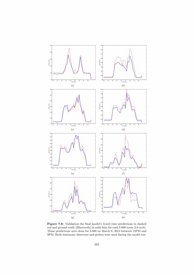
12 13 14 15 16 17 18 19 2050

100

150

200

250

300

time (hour)

trav

el ti

me

(s)

(a)

12 13 14 15 16 17 18 19 2050

100

150

200

250

300

350

400

450

time (hour)

trav

el ti

me

(s)

(b)

12 13 14 15 16 17 18 19 2050

100

150

200

250

300

350

time (hour)

trav

el ti

me

(s)

(c)

12 13 14 15 16 17 18 19 2050

100

150

200

250

300

350

400

450

time (hour)

trav

el ti

me

(s)

(d)

12 13 14 15 16 17 18 19 2050

100

150

200

250

300

350

400

450

500

550

time (hour)

trav

el ti

me

(s)

(e)

12 13 14 15 16 17 18 19 2050

100

150

200

250

300

350

time (hour)

trav

el ti

me

(s)

(f)

12 13 14 15 16 17 18 19 2050

100

150

200

250

300

350

time (hour)

trav

el ti

me

(s)

(g)

12 13 14 15 16 17 18 19 20 2140

60

80

100

120

140

160

180

200

220

240

time (hour)

trav

el ti

me

(s)

(h)

Figure 7.6: Validation the final model’s travel time predictions in dashedred and ground truth (Bluetooth) in solid blue for each I-880 route 2-9 (a-h).These predictions were done for I-880 on March 9, 2012 between 12PM and9PM. Both stationary detectors and probes were used during the model run.

101

As a final validation perspective of the model is the velocity field (given inmiles per hour) in Figure 7.7 considered. Note that this is the actual modeloutput for the 9th of March prior to aggregation.

time

posi

tion

(mile

)

2PM 4PM 6PM 8PM

1

2

3

4

5

6

7

8

9

10

0

10

20

30

40

50

60

70

80

Figure 7.7: Qualitative validation of the actual (non-aggregated) I-880model output, a velocity field given in miles per hour on March 9, 2012between 12PM and 9PM. Both stationary detectors and probes were usedduring the model run. Standard fundamental diagrams were used with thecalibrated parameters.

7.2.2 Global and type-differentiated calibration frameworkusing estimated fundamental diagrams: Interstate880, CA

The final calibration result for the actual calibration date is depicted in Figure7.8 as the aggregated model output on the right hand side versus the groundtruth on the left hand side.

Figure 7.9 shows the validation results, i.e. the aggregated model outputfor March 9, 2012 using the calibrated parameter set. This is the outcome ofthe process that was proposed in Section 6.3.2. Travel time graphs are given inFigure 7.10 for the same date, time and aggregation period. Table 7.6 shows themean absolute percentage errors for each route on both of the calibration andvalidation dates. The values within parenthesis in the same table are the MAPE-metrics for the I-880 model that was calibrated using standard fundamentaldiagrams and that was presented in the previous section.

Finally there is the actual model output for the validation date, i.e. thevelocity field for I-880 northbound as predicted by the calibrated model usingestimated fundamental diagrams and calibrated parameters. This actual modeloutput, the velocity field is given in Figure 7.11.

102

time

posi

tion

(mile


13:00:00 14:15:00 15:30:00 16:45:00 18:00:00 19:15:00 20:30:00

1.09275

2.09275

3.09275

4.09275

5.09275

6.09275

7.09275

8.09275

9.09275

10.0927

0

10

20

30

40

50

60

70

80

time

posi

tion

(mile

)


13:00:00 14:15:00 15:30:00 16:45:00 18:00:00 19:15:00 20:30:00

1.09275

2.09275

3.09275

4.09275

5.09275

6.09275

7.09275

8.09275

9.09275

10.0927

0

10

20

30

40

50

60

70

80

1

Figure 7.8: Outcome of the calibration effort. Ground truth (left) is com-pared to the aggregated model output (right) for I-880 northbound on March14, 2012. Stationary detectors and probes were used during this calibrationrun together with estimated fundamental diagrams.

time

posi

tion

(mile

)

Aggregated Velocity (mph) for nid 340 with agg. period 15 time between 2012−03−09 12:00 and 2012−03−09 21:00

13:00:00 14:15:00 15:30:00 16:45:00 18:00:00 19:15:00 20:30:00

1.09275

2.09275

3.09275

4.09275

5.09275

6.09275

7.09275

8.09275

9.09275

10.0927

0

10

20

30

40

50

60

70

80

time

posi

tion

(mile

)


13:00:00 14:15:00 15:30:00 16:45:00 18:00:00 19:15:00 20:30:00

1.09275

2.09275

3.09275

4.09275

5.09275

6.09275

7.09275

8.09275

9.09275

10.0927

0

10

20

30

40

50

60

70

80

1

Figure 7.9: Validation results for the I-880 model. Ground truth (left)is compared to the aggregated model output (right) for I-880 northboundon March 9, 2012. Stationary detectors and probes were used during thiscalibration run together with estimated fundamental diagrams.

103

Table 7.6: Calibrated model performance in relation to Bluetooth groundtruth on a route-by-route basis for the validation date March 9, 2012 andthe calibration date March 14, 2012. Both stationary detectors and probesof type B were used during these model runs. The corresponding metrics forthe previous I-880 model, where standard fundamental diagrams were usedare included in parenthesis.

Route MAPE (%) March 9 MAPE (%) March 141 (-) 5.3 (4.1) 10.0 (5.3)2 (a) 14.0 (9.7) 11.0 (8.6)3 (b) 16.0 (20.0) 15.0 (13.0)4 (c) 9.4 (4.7) 7.4 (6.5)5 (d) 11.0 (12.0) 11.0 (10.0)6 (e) 12.0 (6.3) 15.0 (8.3)7 (f) 18.0 (15.0) 19.0 (17.0)8 (g) 13.0 (10.0) 12.0 (11.0)9 (h) 14.0 (11.0) 21.0 (14.0)Model 11.6 (9.5) 13.4 (10.1)

104

12 13 14 15 16 17 18 19 2050

100

150

200

250

300

time (hour)

trav

el ti

me

(s)

(a)

12 13 14 15 16 17 18 19 2050

100

150

200

250

300

350

400

time (hour)

trav

el ti

me

(s)

(b)

12 13 14 15 16 17 18 19 2050

100

150

200

250

300

350

400

time (hour)

trav

el ti

me

(s)

(c)

12 13 14 15 16 17 18 19 2050

100

150

200

250

300

350

400

450

500

550

time (hour)

trav

el ti

me

(s)

(d)

12 13 14 15 16 17 18 19 200

100

200

300

400

500

600

700

800

time (hour)

trav

el ti

me

(s)

(e)

12 13 14 15 16 17 18 19 2050

100

150

200

250

300

350

400

time (hour)

trav

el ti

me

(s)

(f)

12 13 14 15 16 17 18 19 2050

100

150

200

250

300

350

time (hour)

trav

el ti

me

(s)

(g)

12 13 14 15 16 17 18 19 20 2140

60

80

100

120

140

160

180

200

220

240

time (hour)

trav

el ti

me

(s)

(h)

Figure 7.10: Validation result, the model’s travel time prediction in dashedred and ground truth (Bluetooth) in solid blue for each I-880 route 2-9 (a-h).These predictions were done for I-880 on March 9, 2012 between 12PM and9PM. Both stationary detectors and probes were used during the model run.Estimated fundamental diagrams were used.

105

time

posi

tion

(mile

)

2PM 4PM 6PM 8PM

1

2

3

4

5

6

7

8

9

10

0

10

20

30

40

50

60

70

80

Figure 7.11: Qualitative validation of the actual (non-aggregated) I-880model output, a velocity field given in miles per hour on March 9, 2012between 12PM and 9PM. Both stationary detectors and probes were usedduring the model run. Estimated fundamental diagrams were used with thecalibrated parameters.

7.2.3 Global calibration framework using estimated fun-damental diagrams: Interstate 15, Ontario, CA

This section presents the results that were acquired following the frameworkpresented in . The complex had not converged after 500 + 30 iterations3, thebest parameter set had a MAPE equal to 7.4 % on the calibration date range10AM-8PM on April 4, 2012.

The aggregated outputs for the validation dates April 3 and 5 are shown infigures 7.13 and 7.15 together with the ground truth for each of these two days.For the sake of comparison is the model output prior to calibration included infigures 7.12 and 7.14.

The performance metric is given on a route-by-route basis in Table 7.7 andfor the model as a whole. The validation dates (April 3 and 5) as well asthe calibration date (Aril 4). Within parenthesis in Table 7.7 is the model’sperformance for each of these three days prior to calibration.

The travel times for each route and validation day are given in Figures 7.16and 7.17. These are the results of the highway model after calibration. Notethat the seventh route was omitted from these figures since that section seldomshows any sign of congestion. All values are given in seconds.

3Some parameters had approach the bounds and were therefore recalibrated, thus the extra30 iterations.

106

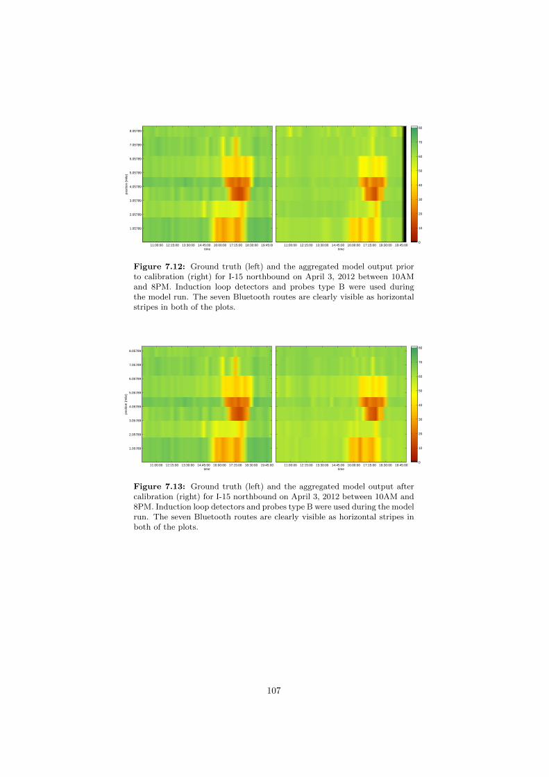
time

posi

tion

(mile


11:00:00 12:15:00 13:30:00 14:45:00 16:00:00 17:15:00 18:30:00 19:45:00

1.05789

2.05789

3.05789

4.05789

5.05789

6.05789

7.05789

8.05789

0

10

20

30

40

50

60

70

80

time

posi

tion

(mile

)


11:00:00 12:15:00 13:30:00 14:45:00 16:00:00 17:15:00 18:30:00 19:45:00

1.05789

2.05789

3.05789

4.05789

5.05789

6.05789

7.05789

8.05789

0

10

20

30

40

50

60

70

80

1

Figure 7.12: Ground truth (left) and the aggregated model output priorto calibration (right) for I-15 northbound on April 3, 2012 between 10AMand 8PM. Induction loop detectors and probes type B were used duringthe model run. The seven Bluetooth routes are clearly visible as horizontalstripes in both of the plots.

time

posi

tion

(mile

)


11:00:00 12:15:00 13:30:00 14:45:00 16:00:00 17:15:00 18:30:00 19:45:00

1.05789

2.05789

3.05789

4.05789

5.05789

6.05789

7.05789

8.05789

0

10

20

30

40

50

60

70

80

time

posi

tion

(mile

)


11:00:00 12:15:00 13:30:00 14:45:00 16:00:00 17:15:00 18:30:00 19:45:00

1.05789

2.05789

3.05789

4.05789

5.05789

6.05789

7.05789

8.05789

0

10

20

30

40

50

60

70

80

1

Figure 7.13: Ground truth (left) and the aggregated model output aftercalibration (right) for I-15 northbound on April 3, 2012 between 10AM and8PM. Induction loop detectors and probes type B were used during the modelrun. The seven Bluetooth routes are clearly visible as horizontal stripes inboth of the plots.

107

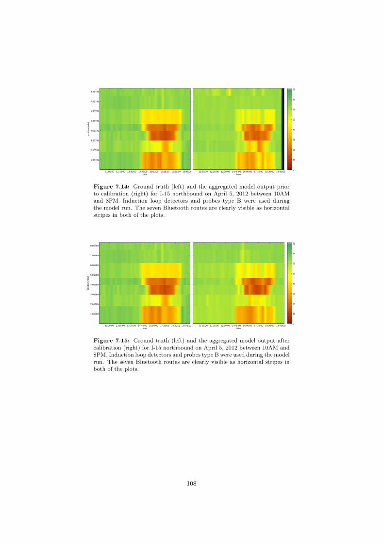
time

posi

tion

(mile


11:00:00 12:15:00 13:30:00 14:45:00 16:00:00 17:15:00 18:30:00 19:45:00

1.05789

2.05789

3.05789

4.05789

5.05789

6.05789

7.05789

8.05789

0

10

20

30

40

50

60

70

80

time

posi

tion

(mile

)


11:00:00 12:15:00 13:30:00 14:45:00 16:00:00 17:15:00 18:30:00 19:45:00

1.05789

2.05789

3.05789

4.05789

5.05789

6.05789

7.05789

8.05789

0

10

20

30

40

50

60

70

80

1

Figure 7.14: Ground truth (left) and the aggregated model output priorto calibration (right) for I-15 northbound on April 5, 2012 between 10AMand 8PM. Induction loop detectors and probes type B were used duringthe model run. The seven Bluetooth routes are clearly visible as horizontalstripes in both of the plots.

time

posi

tion

(mile

)


11:00:00 12:15:00 13:30:00 14:45:00 16:00:00 17:15:00 18:30:00 19:45:00

1.05789

2.05789

3.05789

4.05789

5.05789

6.05789

7.05789

8.05789

0

10

20

30

40

50

60

70

80

time

posi

tion

(mile

)


11:00:00 12:15:00 13:30:00 14:45:00 16:00:00 17:15:00 18:30:00 19:45:00

1.05789

2.05789

3.05789

4.05789

5.05789

6.05789

7.05789

8.05789

0

10

20

30

40

50

60

70

80

1

Figure 7.15: Ground truth (left) and the aggregated model output aftercalibration (right) for I-15 northbound on April 5, 2012 between 10AM and8PM. Induction loop detectors and probes type B were used during the modelrun. The seven Bluetooth routes are clearly visible as horizontal stripes inboth of the plots.

108

Table 7.7: Calibrated model performance in relation to Bluetooth groundtruth on a route-by-route basis for the validation dates April 3 and 5, 2012and the calibration date April 4, 2012. A value within parenthesis gives theperformance prior to the calibration effort.

Route MAPE (%) April 3 MAPE (%) April 5 MAPE (%) April 41 (a) 14.0 12.0 12.02 (b) 6.7 9.6 5.83 (c) 8.4 9.0 7.04 (d) 10.0 12.0 10.05 (e) 5.5 7.9 8.76 (f) 4.5 3.8 3.47 (-) 2.0 2.4 2.4Model 7.4 (8.2) 8.5 (9.7) 7.4 (9.3)

109

10 12 14 16 18100

150

200

250

300

350

time (hour)

trav

el ti

me

(s)

(a)

10 12 14 16 18 2050

60

70

80

90

100

110

120

130

time (hour)

trav

el ti

me

(s)

(b)

10 12 14 16 18 200

50

100

150

200

250

300

time (hour)

trav

el ti

me

(s)

(c)

10 12 14 16 18 2040

60

80

100

120

140

160

180

time (hour)

trav

el ti

me

(s)

(d)

10 12 14 16 18 2040

60

80

100

120

140

160

time (hour)

trav

el ti

me

(s)

(e)

10 12 14 16 18 2070

80

90

100

110

120

130

140

150

time (hour)

trav

el ti

me

(s)

(f)

Figure 7.16: Validation of model predictions of the travel time in red andground truth (Bluetooth) in blue for each I-15 route 1-6 (a-f). These predic-tions were done for April 3, 2012 between 10AM and 8PM. Both stationarydetectors and probes type B were used during the model run.

110

10 12 14 16 18100

150

200

250

300

350

time (hour)

trav

el ti

me

(s)

(a)

10 12 14 16 18 2050

60

70

80

90

100

110

120

130

140

time (hour)

trav

el ti

me

(s)

(b)

10 12 14 16 18 200

50

100

150

200

250

300

time (hour)

trav

el ti

me

(s)

(c)

10 12 14 16 18 2040

60

80

100

120

140

160

180

200

220

time (hour)

trav

el ti

me

(s)

(d)

10 12 14 16 18 2040

50

60

70

80

90

100

110

120

130

140

time (hour)

trav

el ti

me

(s)

(e)

10 12 14 16 18 2075

80

85

90

95

100

time (hour)

trav

el ti

me

(s)

(f)

Figure 7.17: Validation of model predictions of the travel time in red andground truth (Bluetooth) in blue for each I-15 route 1-6 (a-f). These predic-tions were done for April 5, 2012 between 10AM and 8PM. Both stationarydetectors and probes type B were used during the model run.

Finally, and as means to enable a more qualitative validation of the model’soutput after calibration is the highway model’s actual output included in figures7.18 and 7.19. These are the velocity fields were the speed is given in miles perhour in space and time.

111

time

posi

tion

(mile

)

10AM 12PM 2PM 4PM 6PM 8PM

1

2

3

4

5

6

7

8

0

10

20

30

40

50

60

70

80

Figure 7.18: Qualitative validation of the actual (non-aggregated) I-15model output, a velocity field given in miles per hour on April 3, 2012between 10AM and 8PM. Both stationary detectors and probes were usedduring the model run. Estimated fundamental diagrams were used with thecalibrated parameters.

time

posi

tion

(mile

)

10AM 12PM 2PM 4PM 6PM 8PM

1

2

3

4

5

6

7

8

0

10

20

30

40

50

60

70

80

Figure 7.19: Qualitative validation of the actual (non-aggregated) I-15model output, a velocity field given in miles per hour on April 5, 2012between 10AM and 8PM. Both stationary detectors and probes were usedduring the model run. Estimated fundamental diagrams were used with thecalibrated parameters.

112

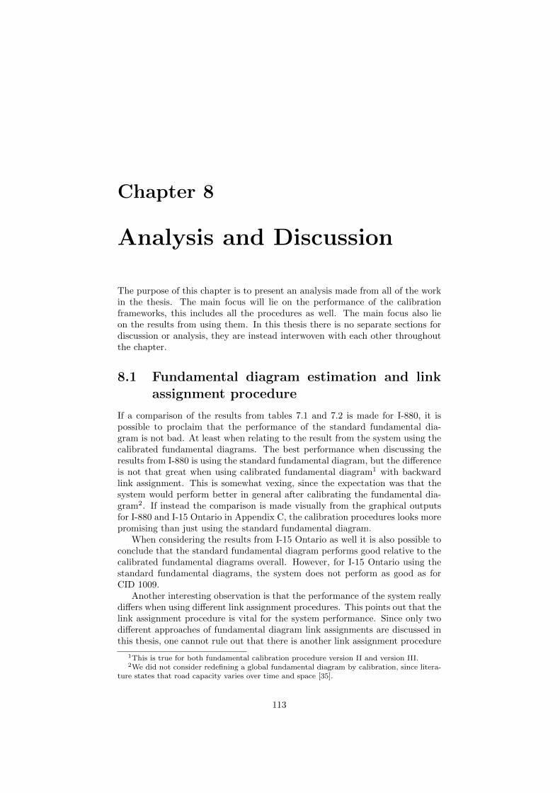
Chapter 8

Analysis and Discussion

The purpose of this chapter is to present an analysis made from all of the workin the thesis. The main focus will lie on the performance of the calibrationframeworks, this includes all the procedures as well. The main focus also lieon the results from using them. In this thesis there is no separate sections fordiscussion or analysis, they are instead interwoven with each other throughoutthe chapter.

8.1 Fundamental diagram estimation and linkassignment procedure

If a comparison of the results from tables 7.1 and 7.2 is made for I-880, it ispossible to proclaim that the performance of the standard fundamental dia-gram is not bad. At least when relating to the result from the system using thecalibrated fundamental diagrams. The best performance when discussing theresults from I-880 is using the standard fundamental diagram, but the differenceis not that great when using calibrated fundamental diagram1 with backwardlink assignment. This is somewhat vexing, since the expectation was that thesystem would perform better in general after calibrating the fundamental dia-gram2. If instead the comparison is made visually from the graphical outputsfor I-880 and I-15 Ontario in Appendix C, the calibration procedures looks morepromising than just using the standard fundamental diagram.

When considering the results from I-15 Ontario as well it is also possible toconclude that the standard fundamental diagram performs good relative to thecalibrated fundamental diagrams overall. However, for I-15 Ontario using thestandard fundamental diagrams, the system does not perform as good as forCID 1009.

Another interesting observation is that the performance of the system reallydiffers when using different link assignment procedures. This points out that thelink assignment procedure is vital for the system performance. Since only twodifferent approaches of fundamental diagram link assignments are discussed inthis thesis, one cannot rule out that there is another link assignment procedure

1This is true for both fundamental calibration procedure version II and version III.2We did not consider redefining a global fundamental diagram by calibration, since litera-

ture states that road capacity varies over time and space [35].

113

that make the system perform better for I-880 when using either version II orversion III of the fundamental diagram calibration procedure.

8.1.1 Calibration framework

The model MAPE for I-880 with the first framework3 and with the standardfundamental diagrams, for the calibration date 9:th of March 2012 is 9.5 %respectively for the validation date 14:th of March is 10.1 %. Whilst withthe second framework4 the model MAPE is for the calibration date 11.6 %respectively 13.4 % for the validation date.

Why the model run with the second framework5 performs worse for I-880,is probably due to the fact that the system in general performs worse withestimated fundamental diagrams, see the results from Table 7.1 and 7.2. It canalso depend on where the stationary sensors are located. The sensors act asa good boundary condition, since the state at these locations almost always isknown. It would therefore probably be better for the system performance tohalt the estimation where the last sensor is placed. We have no suggestions fornetworks without stationary sensors though.

The model MAPE for I-15 Ontario is 8.5 % for the calibration date 4:th ofApril, 7.4 % for the validation dates 3:rd and 5:th of April. Why the modelperformance is better than for I-880 is probably due to less congestion, seefigure C.17(a), C.18(a) and C.19(a). Less congestion practically means that thesystem does not need to estimate the changes in the traffic state. So therefore,as long as the free flow conditions are calibrated right, the model performancewill be more accurate for a network where the system have less congestion ingeneral, at least when comparing to a more congested network.

It is also very noteworthy, that the complex method does not converge whencalibrating I-15 Ontario. This means that the model result is probably going toimprove, when run over more iterations. Since the time for calibrating the modelwas limited and system limitations this was the best that we could do. But, itwould have been very interesting to see how well the model performance wouldbeen when the complex method converges. Why the complex method does notconverge could depend on several different things. One is that the convergencecriteria can be set to be too exact. Another can be that the amount of iterationsis too few.

Even though the second framework performs less well than the first, esti-mating the fundamental diagrams has its advantages. The advantage is in theability to adapt the capacity with respect to actual measurements, rather thantrust that the standard fundamental diagram is accurate. When calibrating anunfamiliar road and the conditions regarding that unfamiliar road (test site I-15Ontario); assuming that the same conditions can be applied from those on I-880can be a false statement and a problem. Therefore adapting the fundamentaldiagrams with respect to local road conditions is a good approach for copingwith this.

3Local and source alternating calibration framework.4Global calibration and type-differentiated calibration framework using estimated funda-

mental diagrams5Global and type-differentiated calibration framework using estimated fundamental dia-

grams.

114

Chapter 9

Conclusion and FutureWork

This chapter will present the conclusion of all the work done in the thesis. In thischapter we will provide suggestions and recommendations of how to calibrate atraffic state space model. Suggested future work will also be presented in thischapter.

It is possible to conclude that this thesis is able to present a framework forcalibrating a state space model. The performance of the calibration frameworkand the results are not as exhaustive as we would have preferred. But all of theresults for the framework points in one direction and that is, with calibrationwe get a higher model accuracy than with the default parameters. Since thecomplex method did not converge, we cannot state that the model is calibrated,but it is possible to state that improvement of the accuracy of the model haveincreased.

The preferable and suggested framework for further use, according to theauthors, is the global and type-differentiated calibration framework using es-timated fundamental diagram. The main reason for this is that the approachwhen calibrating parameters is more general and adaptive than with the otherframework. Even considering it does not perform as good when compared tothe other framework, but the differences between the output is not substantiallylarge. There is still an improvement when using this framework when comparedto the default parameters in the system.

It is also possible to conclude that there is still much work left to do, es-pecially regarding testing and further development of the framework. Not onlytesting more calibration procedures, but also testing the framework with othersimilar state space models as well e.g. the density based cell transmission model.The suggested main area for further research is certainly testing the framework.Another relevant subjects of research would be to test other procedures forassigning fundamental diagrams.

Another interesting area for further research, is to explore the impact ofdifferent modifications to the Mobile Millennium. One of this would be testingother version than the Hyperbolic Linear fundamental diagram.

115

Bibliography

[1] A. Bayen, J. Butler, and A. D. Patire, Mobile Millennium Final Report.California Center for Innovative Transportation Institute of TransportationStudies University of California, Berkeley, 2011.

[2] D. B. Work, S. Blandin, O. Tossavainen, B. Piccoli, and A. M. Bayen, “Atraffic model for velocity data assimilation,” Applied Mathematics ResearcheXpress, vol. 2010, pp. 1–35, April 2010.

[3] M. J. Lighthill and G. B. Whitham, “On kinetic wave ii: a theory of traf-fic flow on crowded roads,” Proceedings of the Royal Society of London,vol. Series A, pp. 317–345, 1955.

[4] P. Richards, “Shockwaves on the highway,” Operations Research, vol. 4,pp. 42–51, 1956.

[5] B. D. Greenshield, “A study of traffic capacity,” Highway Research Board,vol. 14, pp. 448–477, 1935.

[6] C. F. Daganzo, “The cell transmission model: a dynamic representation ofhighway traffic consistent with the hydrodynamic theory.,” TransportationResearch Part B 28, no, vol. 28, pp. 269–287, 1994.

[7] C. J. Herrera and A. M. Bayen, “Incorporation of lagrangian measurementsin freeway trafic state estimation,” Transportation Research Part B, vol. 44,pp. 460–481, 2012.

[8] C. Bardos, A. Le Roux, and J. Nedelec, “First order quasilinear equationswith boundary conditions,” Communication in Partial Differential Equa-tions, vol. 4, pp. 1017–1034, 1979.

[9] C. F. Daganzo, “The cell transmission model. part i: A simple dynamicrepresentation of highway traffic,” California Path Program Institute ofTransportation Studies, University of California, Berkeley, 1993.

[10] G. Evensen, “Sequential data assimilation with a nonlinear quasi-geostrophic model using monte carlo methods to forecast error statistics,”Journal of Geophysical Research, vol. 99, pp. 10,143–10,162, May 1994.

[11] R. E. Kalman, “A new approach to linear filtering and prediction prob-lems,” Transactions of the ASME–Journal of Basic Engineering, vol. 82,no. Series D, pp. 35–45, 1960.

116

[12] G. Evensen, Data Assimilation: The Ensemble Kalman Filter. Springer-Verlag Berlin Heidelberg, 2 ed., 2009.

[13] P. J. van Leeuwen and G. Evensen, “Assimilation data and inverse methodsin terms of a probabilistic formulation,” Monthly Weather Review, vol. 124,pp. 2898–2913, 1996.

[14] G. Evensen, “The ensemble kalman filter for combined state and parameterestimation,” IEEE Control Systems Magazine, vol. 29, pp. 83–104, 2009.

[15] G. Evensen, “The ensemble kalman filter: Theoretical formulation andpractical implementation,” Ocean Dynamics, vol. 53, pp. 343–367, 2003.

[16] G. Burgers, P. J. van Leeuwen, and G. Evensen, “Analysis scheme in the en-semble kalman filter,” American Meterological Society, vol. 126, pp. 1719–1724, 1998.

[17] B. Hellinga, “Requirement for the calibra-tion of traffic simulation models.” Unpublished,http://www.civil.uwaterloo.ca/bhellinga/publications/Publications/CSCE-1998-Calibration.PDF, accessed 2012-07-31.

[18] D. Ngoduy and M. J. Maher, “Calibration of second order traffic modelsusing continuous cross entropy method,” Transportation Research Part C,vol. 24, pp. 102–121, 2012.

[19] H. Rakha, B. Hellinga, M. Van Aerde, and W. Perez, “Systematic ver-ification, validation and calibration of traffic simulation models.” Paperpresented at the Annual Meeting, TRB, Washington, DC, 1996.

[20] B. Park and H. Qi, “Development and evaluation of a calibration and val-idation procedure for microscopic simulation models,” tech. rep., VirginiaTransportation Research Council, 2004.

[21] G. Dervisoglu, G. Gomes, J. Kwon, R. Horowitz, and P. Varaiya, “Auto-matic calibration of the fundamental diagram and empirical observations oncapacity,” 2009. Presented at 88th Annual Meeting of the TransportationResearch Board, Washington, D.C., 2009.

[22] L. Munoz, X. Sun, D. Sun, G. Gomes, and R. Horowitz, “Methodologi-cal calibration of the cell transmission model,” in Proceeding of the 2004American Control Conference, vol. 1, pp. 798–803, 2004.

[23] M. Cremer and M. Papageorgiou, “Parameter identification for a trafficflow model,” Automatica, vol. 17, no. 6, pp. 837–843, 1981.

[24] Z. Li, H. Liu, and J. Li, “A calibration and validation procedure for micro-scopic simualtion model,” in Intelligent Transportation Systems (ITSC),2010 13th International IEEE Conference, pp. 563–568, InternationalIEEE, September 2010.

[25] R. Dowling, A. Skabardonis, and V. Alexiadis, “Traffic analysis toolboxvolume iii: Guidelines for applying traffic microsimulation software,” tech.rep., Dowling Associates, Inc., 2004.

117

[26] C. Braban-Ledoux, “Metacor - a macroscopic modelling tool for corridorapplication to the stockholm test site,” tech. rep., The Royal Institute ofTechnology, Center For Traffic Engineering & Traffic Simulation, 2000.

[27] A. Kotsialos, Y. Pavlis, M. Papageorgiou, and G. Vardaka, “Daccord -development and application of co-ordinated control of corridors, annexb,” tech. rep., Hague Consulting Group, 1997.

[28] A. Kotsialos, M. Papageorgiou, C. Diakaki, Y. Pavlis, and F. Middelham,“Traffic flow modeling of large-scale motorway networks using the macro-scopic modeling tool metanet,” IEEE Transactions on Acoustics Speech andSignal Processing on Intelligent Transportation Systems, vol. 3, pp. 282–292, December 2002.

[29] Highway Capacity Manual. Transportation Research Board, 2000.

[30] P. Boyd and L. Vandenberghe, Convex Optimization. Cambridge UniversityPress, 2004.

[31] G. Blom, Sannolikhetsteori och statistikteori med tillampningar. Studentlit-teratur AB, 2005.

[32] M. J. Box, “A new method of constrained optimization and a comparisonwith other methods,” The Computer Journal, vol. 8, pp. 42–52, 1965.

[33] J. Farkas and K. Jarmai, Analysis and Optimum Design of Metal Struc-tures. A.A. Balkema Publishers, 1997.

[34] J. Andersson, Multiobjective Optimization in Engineering Design - Appli-cations to Fluid Power Systems. PhD thesis, Linkopings universitet, 2001.

[35] C. Antoniou, B. R., J. Barcelo, M. Ben-Akiva, H. Hanabusa, R. Hoiguchi,N. Koutsopoulos, H., D. Krajzewicz, M. Kuwahara, R. Liu, P. Vortisch,Y. Wang, and Q. Yang, Fundamentals of Traffic Simulation. SpringerSience, 2010.

118

Appendix A

Identified Parameters

This appendix present the parameters found during the system analysis. Allparameters are divided sections depending on which class they belong to inthe system structure. Thereafter the parameters are sorted into classes. Allparameters found are presented below. The parameters which are not directlycorrelated (or have not found the correlating interpretation) to the literatureare denoted as ϕi where i denotes the ith parameter found.

Measurement loader

Timers

ϕ1 = swedish lag.This timer makes sure that there is time enough for the system to fill thedatabase with filtered data. Current value is set to 300f (seconds).Code:

if (Monitor.get db env().equalsIgnoreCase(”kth01”)) {float swedishLag = 300f;//FIXME: hard coded value

...}

ϕ2 = Seconds Since Last Fixed Measure.This timer sets how long time it is required for resetting the confidences. Currentvalue set to 180f (seconds).Code:

if (secondsSinceLastFixedMeas > 180f) {//FIXME: hard coded valueresetConfidences = true;

}

ϕ3 = interval + 240fThe timer is used when getting Probe A speeds. The purpose of timer is prob-ably used because of the same reasons as the Swedish lag timer, which is imple-mented due to some system lag.Code:

if (loadProbes) {

119

...Probe A Speed = DataType.Probes A Feed.getSpeeds(net, time, interval +240f); //pre filter for probe B speeds and adding the std

...}

Confidence parameters

ϕ4 = Link ConfidenceThis parameter is for setting the default confidence on a link when creating theHashmap. Default value is set to 0.025.Code:

//Create Hashmap for link confidencesHashMap< Integer, Float> linkConfidenceMap = new HashMap< Integer,Float> ();for (Integer linkId : this.id) {

linkConfidenceMap.put(linkId, 0.025f);//FIXME: hard coded value}

ϕ5 = PeMS Confidence.If there is a PeMS on the link, then set the confidence in the Hashmap to ϕ5.Current value of 0.5.Code:

//change confidence to 0.5 if pems data is in the linkfor (Datum.Speed pemsSpeedMeas : pemsSpeed) {

linkConfidenceMap.put(pemsSpeedMeas.spot.link.id, 0.5f);//FIXME: hard coded value

}

ϕ6 = Radar Confidence.Sets the confidence if radar data is available on the link. The current defaultvalue is 0.5.Code:

//change confidence to 0.5 if radar data is in the linkfor (Datum.Speed radarSpeedMeas : radarSpeed) {

linkConfidenceMap.put(radarSpeedMeas.spot.link.id, 0.5f);//FIXME: hard coded value

}

ϕ7 = info24radar(Note: The same type as radar confidence).This parameter is mainly for the Swedish system. Set the confidence on the linkif not a radar is present. Current set value is 0.0.Code:

//change confidence to 0.5 if radar data is in the linkfor (Datum.Speed info24SpeedMeas : info24Speed) {

linkConfidenceMap.put(info24SpeedMeas.spot.link.id, 0f);//FIXME: hard coded value

}

120

ϕ8 = Probe B Speed Confidence (is it deviation?).Sets the confidence if a Probe B is on a link at a current spot with a currentspeed during a certain time. Current value 4.0.Code:

if (ds.speed > 1f) {dsArrayList.add(new Datum.Speed(ds.time, ds.spot, ds.speed, 4F));//FIXME: hard coded value

...}ϕ9 = confidence checker for B Probes.Checks whether the confidence is below a certain level. If it is then increase theconfidence with a certain amount. Current value 0.05.Code:

if (prevConfidence < (1f - 0.05f)) {//FIXME: hard coded valuelinkConfidenceMap.put(linkId, prevConfidence + 0.05f);//FIXME: hard coded value

}ϕ10 = Add confidence.Adds to current confidence if probe B is on the link. Current value is 0.05.Code:


}ϕ11 = Probe A Speed Confidence (standard deviation?).Sets the confidence if a Probe A is on a link at a current spot with a currentspeed during a certain time. Current value 4.0.Code:

if (ds.speed > 1f) {//FIXME: hard coded valuedsArrayList.add(new Datum.Speed(ds.time, ds.spot, ds.speed, 4F));//FIXME: hard coded value

...}ϕ12 = confidence checker (Probe A).Checks whether the confidence is below a certain level. If it is then increase theconfidence with a certain step. Current value 0.05.Code:


}ϕ13 = add confidence (Probe A).adds to the confidence a certain amount. Current value 0.05.Code:

121


}

ϕ14 = confidence reset value.If no data can be found for a certain time interval, then reset according to ϕ14.Current value is set to 0.0.Code:

//if no fixed sensor data for the last 3 minutes:if (resetConfidences) {

for (Integer linkId : this.id) {linkConfidenceMap.put(linkId, 0f);

}}

ϕ15 = measurementNoiseCov[ii][ii] = stdev != null ? Math.pow(stdev, 2) : 16.0;Set the diagonal in the covariance matrix. Either Math.pow(stdev, 2) or to 16.0.Code:

for (int ii = 0; ii < numberOfSpeedMeasurements; ii++) {measurements[ii] = speedData.get(ii).speed;Float stdev = speedData.get(ii).stdDev;measurementNoiseCov[ii][ii] = stdev != null ? Math.pow(stdev, 2) : 16.0;//FIXME: hard coded value

}

Other parameters

ϕ16 = Localization distance.Sets how far the localization operator should check for neighbouring edges. Cur-rent value 100.0.Code:

this.localizationDistance = 100f;//FIXME: hard coded value

Estimate Manager

Timers

ϕ17 = Get data interval timer.This timer is for setting the get data interval timer to a default value. Thisvalue should probably depend on how much lag the system needs to filter andstore measurements. Current value set to 180.0.Code:

if (tempgetdatainterval != null) {this.get data interval = tempgetdatainterval;

}else {

this.get data interval = 180.0f;//FIXME: hard coded value

122

...}

Statistic Based Parameters

ϕ18 = Model Error Mean.If not the model error mean can be found in the data base then set it to adefault value. Current default value is 0.0.Code:

try {modelErrorMean = this.network.attributes.getDouble(”highway modelErrorMean”);if (null == modelErrorMean) throw new NetconfigException(null, null);

}catch (NetconfigException ex) {

modelErrorMean = 0d;}

ϕ19 = Model Error Covariance.If not the model error covariance can be found in the data base, then set it toa default value. Current is 0.1.Code:

try {modelErrorCov = this.network.attributes.getDouble(”highway modelErrorCov”);if (null == modelErrorCov) throw new NetconfigException(null, null);

}catch (NetconfigException ex) {

modelErrorCov = 0.1d;}

Velocity Flux Function Experimental

CTM-v model parameters

ϕ20 = Speed tolerance.The purpose of this speed tolerance parameter is to set the difference betweenthe free flow speed and the critical speed vc. Current value is set to 2 m/s.Code:

double vtolerance = 2f; //FIXME: hard coded value

ϕ21 = Critical speed.This parameters purpose is to indicate at which speed the critical flow anddensity occurs. Current default value is 26 m/s.Code:

double vcritical = 26f; //FIXME: hard coded value

123

Gudnov Link


ϕ22 = Parameter for increasing the free flow speed.In the Gudnov Link class there is a procedure called getFreeFlowSpeed. Thisprocedure fetches the free flow speed and adds speed for some apparent reason.Current value added = (3 / 2.23693629).Code:

public double getFreeFlowSpeed() {return this.freeFlowSpeed + (3 / 2.23693629);//FIXME: hard coded value

}

Flow Model Network


ϕ23 = Shock wave speed.The speed for how fast the shock wave travels are set in the flow model networkclass. Current value is -5.36448 m/s.Code:

public static final double shockWaveSpeed = -5.36448;//FIXME: hard coded value.

ϕ24 = Maximum density.Sets the maximum density per lane. Current value is 0.12430080 cars/m.Code:

public static final double rhoMax = 0.124300808; //0.108763207;//FIXME: hard coded value.

Flow Model Runner


ϕ25 = initialVelocitySigma.This parameter provides an interface of propagating the velocity field forward.Code:

private final double initialVelocitySigma = 1;//FIXME: hard coded value.

ϕ26 = Free Flow Speed Correction.This parameter changes the Free Flow Speed for the initial states. Current valueis set to - 0.1 m/s.Code:

initState[ii] =entry.getValue().getFreeFlowSpeed() - 0.1

Parameter Store

The split ratios, number of lanes and free flow speed can be hard coded in thisclass.

124

Network (Database)

EnKF Parameters

ϕ27 = Highway model error mean.Sets the default model error mean. Current value 0.5.

ϕ28 = Highway error covariance.Sets the default model error covariance. Current value is set to 2.

125

Appendix B

Bluetooth Deployment

This appendix shows detailed maps as well as maps with overview over theBluetooth deployments.

Figure B.1: A map presenting an overview of the Bluetooth deploymenton Interstate 880, CA and the surroundings areas. Retrieved on September22, 2012 from the webpage maps.google.com

126

Figure B.2: A more detailed map of the Bluetooth deployment on In-terstate 880, CA. Retrieved on September 22, 2012 from the webpagemaps.google.com

127

Figure B.3: The map show an overview of the Bluetooth deployment onI-15 Ontario, CA and the surroundings areas. Retrieved on September 22,2012 from the web page maps.google.com

128

Figure B.4: A detailed map over the Bluetooth deployment on I-15 Ontario, CA. Retrieved on September 22, 2012 from the web pagemaps.google.com

129

Appendix C

Fundamental DiagramCalibration Results

This appendix contains a all of the space mean speed diagrams from running thesystems with all of the configurations for the fundamental calibration procedure.This as well as all of the reference space mean speed diagrams from the Bluetoothand running the highway model with default parameters.

I-880 Northbound

(a) (b) (c)

(d) (e) (f)

Figure C.1: Shows the space mean speed for the calibration methods andthe ground truth from running the highway model on test site I-880. Theaggregation period is 15 minutes over the time period from 2012-03-03 00:00-24:00. C.1(a) shows the ground truth. C.1(b) use the ad-hoc calibration.C.1(c) and C.1(e) use the fundamental diagrams from version III with theforward respectively backward link assignment. C.1(d) and C.1(f) use thefundamental diagrams from version II with the forward respectively back-ward link assignment.

(a) (b) (c)

(d) (e) (f)


(a) (b) (c)

(d) (e) (f)


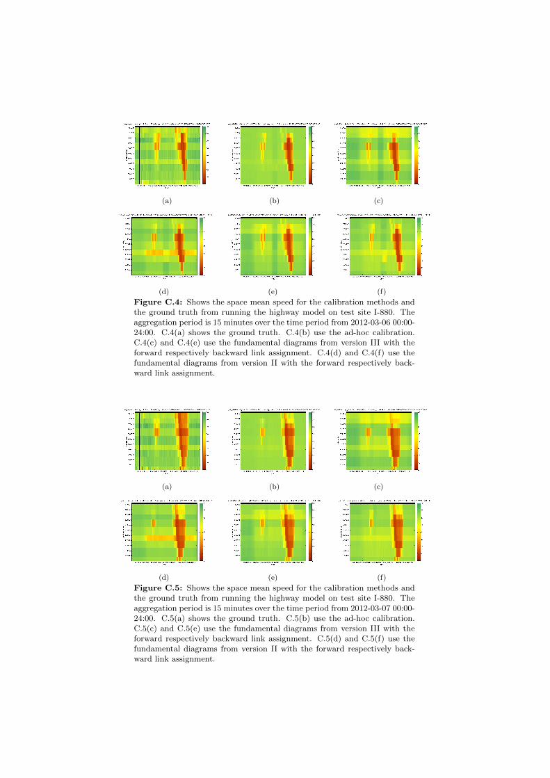
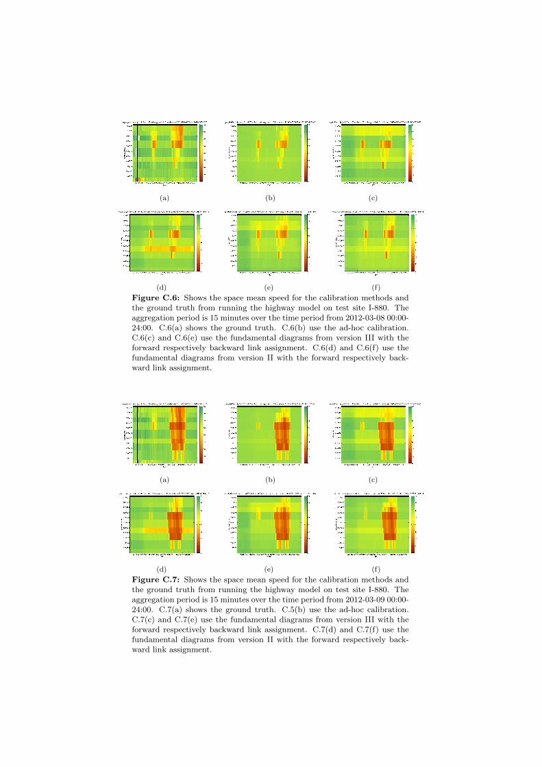
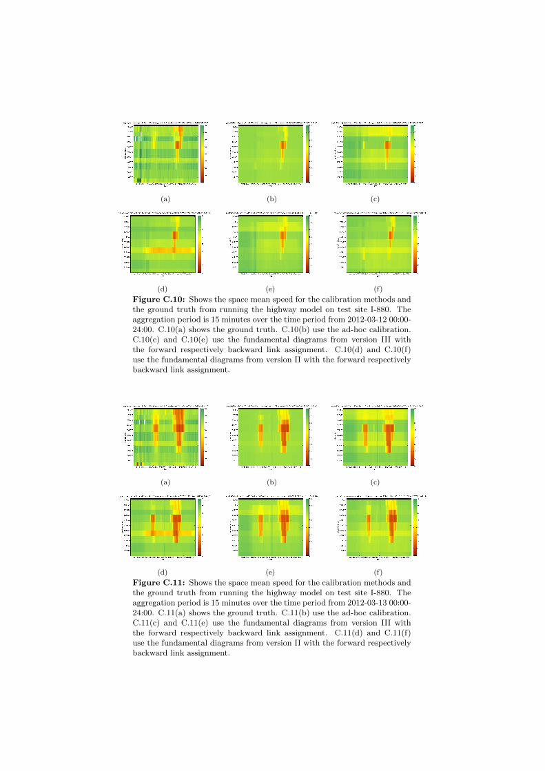
(a) (b) (c)

(d) (e) (f)

Figure C.10: Shows the space mean speed for the calibration methods andthe ground truth from running the highway model on test site I-880. Theaggregation period is 15 minutes over the time period from 2012-03-12 00:00-24:00. C.10(a) shows the ground truth. C.10(b) use the ad-hoc calibration.C.10(c) and C.10(e) use the fundamental diagrams from version III withthe forward respectively backward link assignment. C.10(d) and C.10(f)use the fundamental diagrams from version II with the forward respectivelybackward link assignment.

(a) (b) (c)

(d) (e) (f)


(a) (b) (c)

(d) (e) (f)


(a) (b) (c)

(d) (e) (f)


136

I-15 Ontario Northbound

(a) (b) (c)

(d) (e) (f)

Figure C.14: Shows the space mean speed for the calibration methodsand the ground truth from running the highway model on test site I-15Ontario. The aggregation period is 15 minutes over the time period from2012-03-31 00:00-24:00. C.14(a) shows the ground truth. C.14(b) use thead-hoc calibration. C.14(c) and C.14(e) use the fundamental diagrams fromversion III with the forward respectively backward link assignment. C.14(d)and C.14(f) use the fundamental diagrams from version II with the forwardrespectively backward link assignment.

137

(a) (b) (c)

(d) (e) (f)


(a) (b) (c)

(d) (e) (f)


138

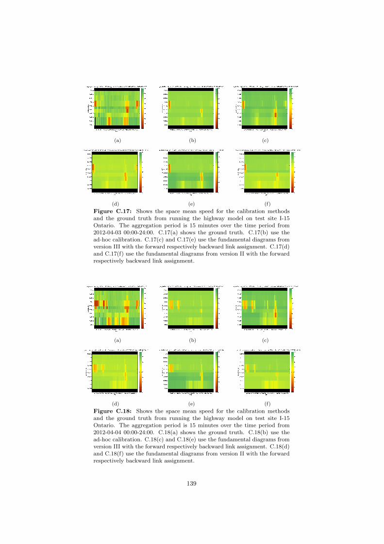
(a) (b) (c)

(d) (e) (f)


(a) (b) (c)

(d) (e) (f)


139

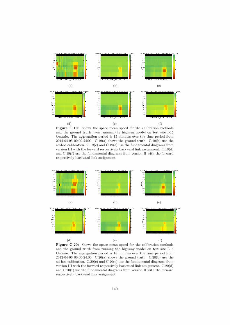
(a) (b) (c)

(d) (e) (f)


(a) (b) (c)

(d) (e) (f)


140

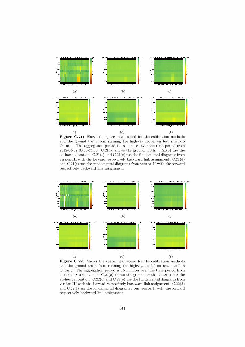
(a) (b) (c)

(d) (e) (f)


(a) (b) (c)

(d) (e) (f)


141

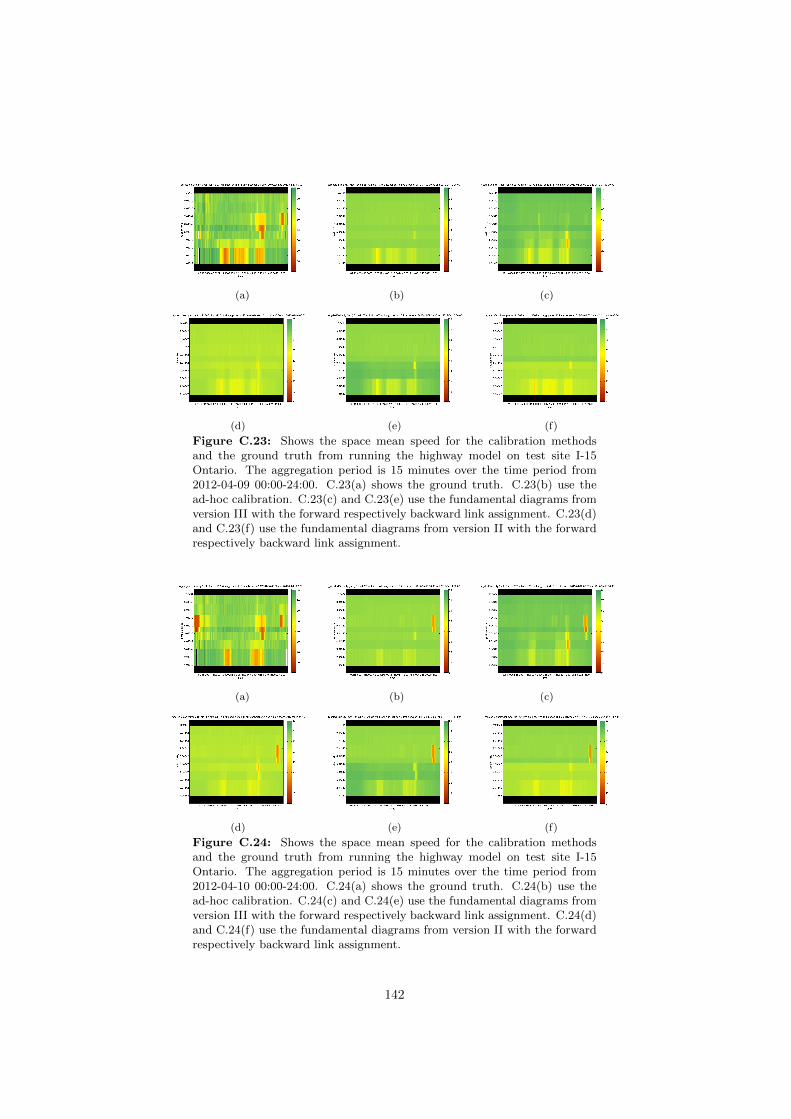
(a) (b) (c)

(d) (e) (f)


(a) (b) (c)

(d) (e) (f)


142

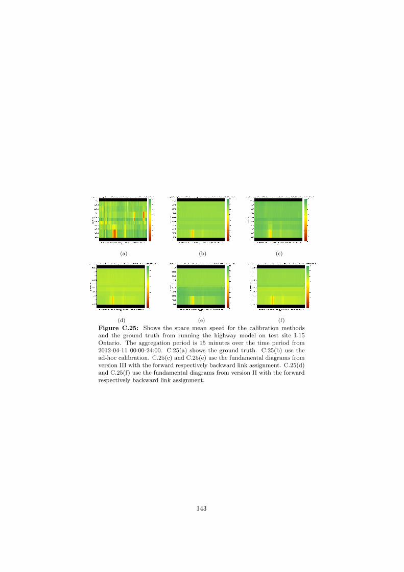
(a) (b) (c)

(d) (e) (f)


143

framework for calibration of a traffic state space model€¦ · 7.2.1 local and source alternating...

Documents