foundaiton on sloping ground

8/12/2019 Foundaiton on Sloping Ground

http://slidepdf.com/reader/full/foundaiton-on-sloping-ground 1/18

(210–VI–NEH, August 2007)

TechnicalSupplement 14Q

Abutment Design for Small Bridges



Part 654

National Engineering Handbook

Abutment Design for Small BridgesTechnical Supplement 14Q

(210–VI–NEH, August 2007)

Advisory Note

Techniques and approaches contained in this handbook are not all-inclusive, nor universally applicable. Designing

stream restorations requires appropriate training and experience, especially to identify conditions where various

approaches, tools, and techniques are most applicable, as well as their limitations for design. Note also that prod-

uct names are included only to show type and availability and do not constitute endorsement for their specific use.

Cover photo: Design of abutments for small bridges requires geotechnical

analysis.

Issued August 2007



(210–VI–NEH, August 2007) TS14Q–i

Contents



Purpose TS14Q–1

NRCS use of bridges TS14Q–1

Bearing capacity TS14Q–1

Flat ground formula ...................................................................................... TS14Q–1

Allowable bearing capacity ........................................................................ TS14Q–2

Sloping ground methods .............................................................................. TS14Q–2

Meyerhof method .......................................................................................... TS14Q–3

Other methods ............................................................................................... TS14Q–4

Selection of shear strength parameters TS14Q–4

Other considerations TS14Q–4

Table TS14Q–1 Terzaghi bearing capacity factors TS14Q–3

Table TS14Q–2 Meyerhof and Hansen bearing capacity factors TS14Q–3

Table TS14Q–3 Meyerhof method design table (cohesionless TS14Q–7

soils)

Table TS14Q–4 Meyerhof method design table (cohesive soils) TS14Q–8

Table TS14Q–5 Undrained shear strength values for saturated TS14Q–9 cohesive soils

Table TS14Q–6 φ´ values for sands TS14Q–10

Figure TS14Q–1 Farm bridge with steel I-beam structural TS14Q–1members and timber strip footing

Figure TS14Q–2 Flood-damaged bridge in EWP program TS14Q–1

Figure TS14Q–3 Forest road culvert acting as fish passage TS14Q–2 barrier

Figure TS14Q–4 Culvert replaced by bridge TS14Q–2



Part 654



TS14Q–ii (210–VI–NEH, August 2007)

Figure TS14Q–5 Definition sketch—strip footing on flat ground TS14Q–2

Figure TS14Q–6 Definition sketch—strip footing adjacent to a TS14Q–3 slope

Figure TS14Q–7 Meyerhof method design charts: ultimate TS14Q–5bearing capacity for shallow footing placed on

or near a slope

Figure TS14Q–8 φ´ values for coarse grained soils TS14Q–11

Figure TS14Q–9 Problem schematic for example problem 1— TS14Q–12 strip footing adjacent to a slope

Figure TS14Q–10 Problem schematic for example problem 2— TS14Q–14 surface load adjacent to a slope



(210–VI–NEH, August 2007) TS14Q–1



Purpose

This technical supplement presents a procedure for

determining the ultimate and allowable bearing capac-

ity for shallow strip footings adjacent to slopes. Addi-

tional guidelines related to scour protection and layout

are also included. Structural design of bridges and

footings is beyond the scope of this document

NRCS use of bridges

Bridges are installed in a variety of U.S. Department of

Agriculture (USDA) Natural Resources ConservationService (NRCS) applications including farm and rural

access roads, livestock crossings, Emergency Water-

shed Protection (EWP) work, and recreation facilities

(figs. TS14Q–1 and TS14Q–2). Bridges installed under

NRCS programs are generally single-span, single-lane

structures and use various simple structural systems

including rail cars, steel I-beams, and timber stringers.

Timber decking is often used to provide the driving

surface. The entire bridge structure is normally sup-

ported by simple strip footings of timber or concrete

on either abutment. The procedure presented in this

technical supplement is appropriate for the design of

abutments for the relatively small bridges typicallyconstructed in NRCS work.

Figure TS14Q–1 Farm bridge with steel I-beam struc-tural members and timber strip footing( Photo courtesy of Ben Doerge)

Figure TS14Q–2 Flood-damaged bridge in EWP program( Photo courtesy of Ben Doerge)

Small bridges may also be used to replace existing cul-

verts that act as barriers to fish passage (figs. TS14Q–3

and TS14Q–4).

Bearing capacity

Flat ground formula

The bearing capacity of strip footings adjacent to

slopes is an extension of the classical theory of bear-

ing capacity for footings on flat ground.

The bearing capacity of a soil foundation is providedby the strength of the soil to resist shearing (sliding)

along induced failure zones under and adjacent to the

footing. Consequently, bearing capacity is a function

of the soil’s shear strength, cohesion, and frictional re-

sistance. Further information on the selection of shear

strength parameters for bearing capacity determina-

tion is included later in this technical supplement.

Bearing capacity formulas for footings on flat ground

have been proposed by Terzaghi (1943) and others

and have the following general form (fig. TS14Q–5 for

definition sketch):



Part 654



TS14Q–2 (210–VI–NEH, August 2007)

q c N q N B Nult c q

= × + × + × × ×1

2γ γ

(eq. TS14Q–1)

where:

q ult

= ultimate bearing capacity (F/L2)

c = cohesion (F/L2)

q = γD = surcharge weight (F/L2)

D = depth of footing below grade (L)

γ = unit weight of soil (F/L3)

B = footing width (L)

Nc, N

q , and N

γ = bearing capacity factors related to

cohesion, surcharge, and friction,

respectively (unitless)

The bearing capacity factors, Nc, Nq , and Nγ, are allfunctions of the soil’s angle of internal friction, φ

(phi). Tables of bearing capacity factors for the flat

ground case are given in tables TS14Q–1 and TS14Q–2

(Bowles 1996). In the classical treatment of bearing ca-

pacity, the foundation is assumed to consist of a single,

homogeneous soil. The basic bearing capacity formula

has been refined by the inclusion of modification fac-

tors to account for such variables as footing shape, in-

clination, eccentricity, and water table effects. See U.S.

Army Corps of Engineers (USACE) EM–1110–1–1905

(1992a) and Bowles (1996) for further description of

these factors.

Allowable bearing capacity

The allowable bearing capacity is determined by ap-

plying an appropriate factor of safety to the ultimate

bearing capacity, q ult

, as determined from the bearing

capacity formula. A factor of safety of 3.0 is often used

with dead and live loads (USACE EM–1110–1–1905,

U.S. Department of Navy Naval Facilities Engineer-

ing Command (NAVFAC) DM 7.2; American Associa-

tion of State Highway and Transportation (AASHTO)

Standard Specifications for Highway Bridges). Settle-

ment of footings should also be checked to verify thatexcessive displacements will not occur. The treatment

of bearing capacity under seismic loading is beyond

the scope of this document.

Sloping ground methods

When the ground surface on one side of the footing is

sloping, as in the case of a bridge abutment adjacent

to a stream channel, the bearing capacity is reduced,

Figure TS14Q–4 Culvert replaced by bridge (Photo cour-tesy of Christi Fisher)

Figure TS14Q–3 Forest road culvert acting as fish pas-sage barrier ( Photo courtesy of Christi

Fisher )

B

q ul t

DSoil: γ , c, φ

Figure TS14Q–5 Definition sketch—strip footing on flatground



TS14Q–3(210–VI–NEH, August 2007)

Part 654



compared to the flat ground case. The reduction is

the result of the loss of some of the available shear

resistance on the sloping side due to the shorteningof the failure surface and decrease in the total weight

acting on the failure surface. The bearing capacity for

footings adjacent to slopes is a function of the same

five variables as for footings on flat ground, with two

additional variables: slope angle (β) and distance from

the shoulder of the slope to the corner of the footing

on the slope side (b) (fig. TS14Q–6).

The reduction in bearing capacity for footings located

adjacent to slopes has been studied extensively, using

both theoretical and physical models. The effect of the

slope is typically accounted for by modifying the bear-

ing capacity factors in the traditional bearing capacityequation for flat ground. As in the classical analysis for

the flat ground case, all methods for sloping ground

are based on the assumption of a homogeneous foun-

dation. A surprisingly wide variation in results may be

observed between the various methods. The findings

of tests on actual physical models are useful in assess-

ing the validity of the various theoretical models.

The Meyerhof method is selected for the purposes of

this technical supplement due to its long-term accep-

tance within the profession and its relative simplicity.

Example calculations are given later.

Meyerhof method

The Meyerhof (1957) method is based on the theory of

plastic equilibrium. It is the oldest method for analyzing

footings adjacent to slopes and has enjoyed wide use.

For example, this method is cited in NAVFAC DM 7.2

φ, deg. Nc Nq Nγ

0 5.7 1.0 0.0

5 7.3 1.6 0.5

10 9.6 2.7 1.2

15 12.9 4.4 2.5

20 17.7 7.4 5.0

25 25.1 12.7 9.7

30 37.2 22.5 19.7

35 57.8 41.4 42.4

40 95.7 81.3 100.4

Table TS14Q–1 Terzaghi (1943) bearing capacity factors

φ, deg. Nc Nq Nγ

(Meyerhof) (Hansen)

0 5.14 1.0 0.0 0.0

5 6.49 1.6 0.1 0.1

10 8.34 2.5 0.4 0.4

15 10.97 3.9 1.1 1.2

20 14.83 6.4 2.9 2.9

25 20.71 10.7 6.8 6.8

30 30.13 18.4 15.7 15.1

35 46.10 33.3 37.2 33.9

40 40.25 64.1 93.6 79.4

Table TS14Q–2 Meyerhof (1957) and Hansen (1970)bearing capacity factors

B

b

Soil: γ , c, φ

q ul t

D

β

Figure TS14Q–6 Definition sketch—strip footing adjacent to a slope



Part 654




and in the AASHTO Standard Specification for Highway

Bridges.

In the Meyerhof (1957) method, the bearing capacity

formula takes the following form:

q c N B Nult cq q

= × + × × ×1

2γ γ (eq. TS14Q–2)

The terms Ncq

and Nγq

are modified bearing capacity

factors in which the effect of surcharge is included.

These factors are determined from design charts repro-

duced in NAVFAC DM 7.2 (fig. TS14Q–7). Procedures

for analyzing rectangular, square, and circular footings,

as well as water table effects, are also presented in

these charts. With the Meyerhof (1957) method, founda-tions of both cohesive and cohesionless soils may be

analyzed, and the footing may be located either on or at

the top of the slope. Values of Nγq

for cohesionless soils

are also given in tabular form in table TS14Q–3 and for

cohesive soils in table TS14Q–4.

Other methods

Many other methods exist for estimating the bearing

capacity of strip footings adjacent to slopes. Bearing

capacity may also be estimated using the principles

of limit equilibrium or finite element analysis. Thedesigner may wish to use more than one method and

compare the results before making a final design deci-

sion. It is recommended that the bearing capacity for

the flat ground case also be computed for reference as

an upper bound.

Selection of shear strengthparameters

Soil shear strength parameters (φ and c) are selectedbased on the assumption that footing loads may be

applied rapidly. If the foundation soils may become

saturated at any time during the life of the structure,

then the design shear strength parameters should be

selected accordingly.

For cohesive soils that develop excess pore pressure

when loaded rapidly (CH, MH, and CL soils), undrained

shear parameters are used. The cohesion (c) is taken

to be the undrained shear strength (su) of the soil in a

saturated condition, and an angle of internal friction (φ)

of zero is used. The undrained shear strength may be

determined from the unconsolidated-undrained (UU)shear test, the unconfined compression (q

u) test, or the

vane shear test. The undrained shear strength may also

be estimated from field tests or index properties. See

table TS14Q–5 to estimate the undrained shear strength

of saturated fine-grained soils from consistency,

standard penetration test (blow count), and liquidity

index.

For cohesionless, free-draining soils that are able to

dissipate excess pore pressure rapidly (SW, SP, GW,

GP, SM, GM, and nonplastic ML soils), the effective

shear strength parameters (φ´ and c´) are used. The

effective cohesion parameter (c´) for cohesionless soilsis either zero or very small and is normally neglected.

The effective angle of internal friction (φ´) may be

determined from shear tests or may be estimated

from generalized charts and tables. See table TS14Q–6

(USACE 1992a) and figure TS14Q–8 (NAVFAC 1982b)

for charts to estimate the effective angle of internal

friction for sands and gravels.

A qualified soils engineer should be consulted when

selecting shear strength parameters for design.

Other considerations

Bridge abutments consisting of soil or other erod-

ible material must be protected against the effects of

scour. Either the footing should be embedded below

the maximum anticipated scour depth or adequate

scour protection must be provided. The embedment

approach is generally not applicable with the shal-

low strip footings normally used with NRCS-designed

bridges. Therefore, scour protection, such as rock

riprap or gabions, should be provided, as necessary, to

prevent erosion of the slope and possible underminingof the footings.

The U.S. Forest Service recommends that bridges with

shallow strip footings be used primarily in stream

channels that are straight and stable, have low scour

potential, and will not accumulate significant debris

or ice. Any additional antiscour measures needed to

ensure the long-term integrity of the bridge abutments

should be incorporated into the design (McClelland

1999).




Part 654



Figure TS14Q–7 Meyerhof method design charts: ultimate bearing capacity for shallow footing placed on or near a slope

β

β

H

Case I:

H D

b B

q

B

q

D

do

Soil: γ , c, φ

Soil: γ , c, φ

90-φ

90-φ

90-φ

do

F o u n d a t i o n f a i l u r e

T o e f a i l u r e

B a s e f a i l u r e

Same criteria as for case I except

that Ncq and Nγ q are obtained from

diagrams for case II

Case II: Continuous footings on slope

Water at do ≥ B

Obtain Ncq from figure 4b for case I with No=0.

Interpolate for values of 0 < D/B < 1Interpolate q u1t between eq and for water at intermediate

level between ground surface and do=B.

H:If

H:If

Obtain Ncq from figure 4b for case I with stability number

Cohesive soil (φ = 0)

Substitute in eq and D for B/2 and Nγ q = 1.

Rectangular, square, or circular footing:

Interpolate for values 0 < D/B < 1 for 0 < No <1 . If No ≥ 1,stability of slope controls ultimate bearing pressure.

Interpolate q u1t between eq and for water intermediate level

between ground surface and do = B. for water at ground surface and sudden

drawdown: Substitute φ´ for φ in eq

Water at ground surface

a

a

b

b

a b

a b

b

q u1t= q u1t

q u1t for finite footing

q u1t for continuous footing×

for continuous footing

as given above

Continuous footing at top of slope

q cNB

Nγ q ult cq T= + γ

2

B ≤

q ult

cNcq sub

BNγ q = + γ

2

No

H

c=

γ

B >

′ = −

φ γ γ

φtan tan1 sub

Τ



Part 654




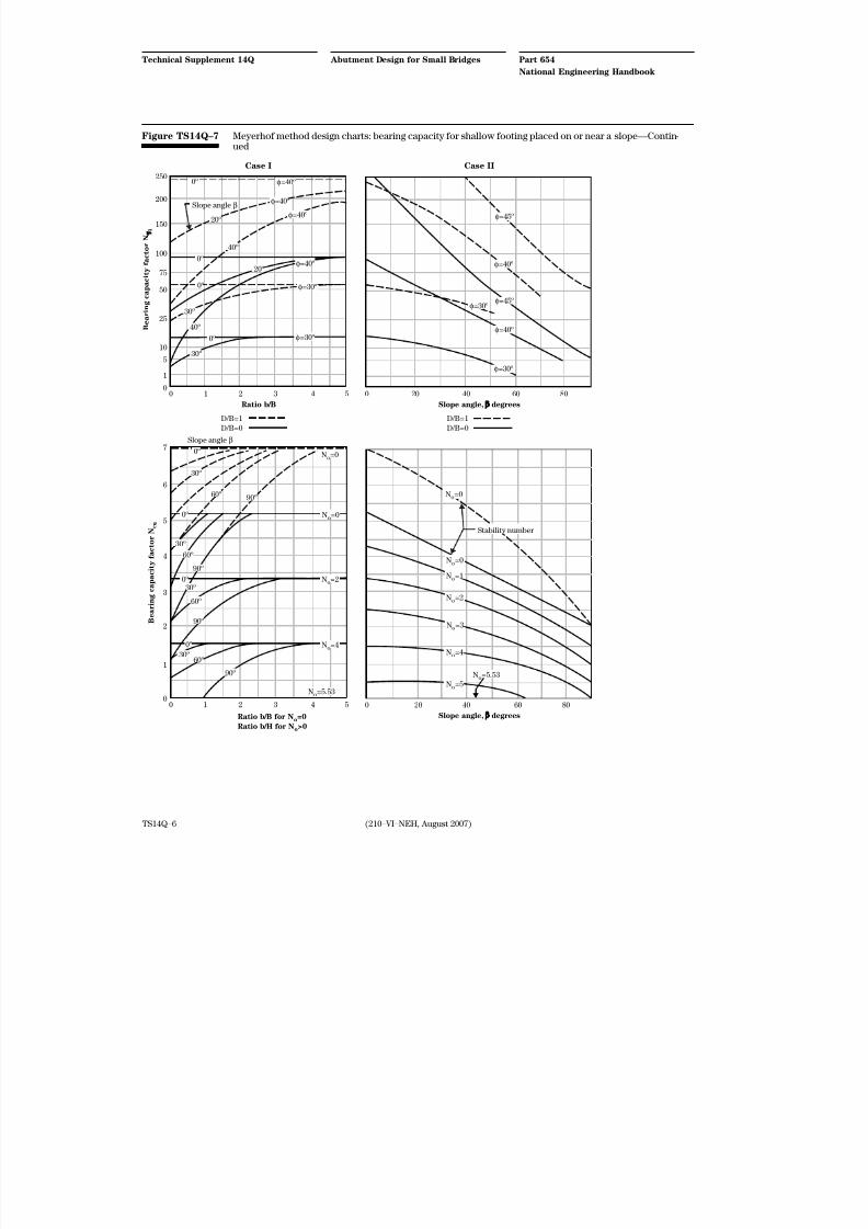
250

Slope angle β

Slope angle, degrees

Case I Case II

20º

0º

0º

0º

0º

40º

30º

20º

40º

30º

φ=40º

φ=40º

φ=40º

φ=45º

φ=45º

φ=40º

φ=30º

φ=30º

φ=30º

φ=30º

φ=40º

φ=40º

200

150

100

75

50

25

10

5

1

00 1 2 3

Ratio b/B

4 5 0 20 40 60 80

0 20 40 60 80

D/B=1

D/B=0

D/B=1

D/B=0

B e a r i n g c a p a c i t y f a c t o r N

7Slope angle β

Stability number

30º

30º

30º

30º

60º

60º

60º

60º

90º

90º

90º

90º

0º

0º

0º

0º

No=0

No=0

No=0

No=0

No=1

No=2

No=3

No=4

No=5

No=2

No=4

No=5.53

No=5.53

6

5

4

3

2

1

00 1 2 3 4 5

Ratio b/B for No=0

Ratio b/H for No>0

B e a r i n g c a p a c i t y f a c t o r N c q

Slope angle, degrees

q

Figure TS14Q–7 Meyerhof method design charts: bearing capacity for shallow footing placed on or near a slope—Contin-ued



T S 1 4 Q– 7

( 2 1 0 –V I – NE H ,A u g u s t 2 0 0 7 )

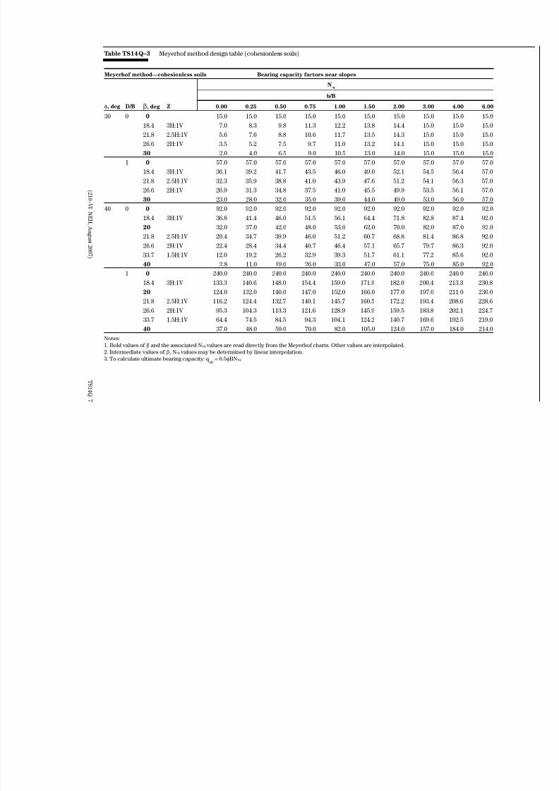
Table TS14Q–3 Meyerhof method design table (cohesionless soils)

Meyerhof method—cohesionless soils Bearing capacity factors near slopes

Nγq

b/B

φ, deg D/B β, deg Z 0.00 0.25 0.50 0.75 1.00 1.50 2.00 3.00 4.00

30 0 0 15.0 15.0 15.0 15.0 15.0 15.0 15.0 15.0 15.0

18.4 3H:1V 7.0 8.3 9.8 11.3 12.2 13.8 14.4 15.0 15.0

21.8 2.5H:1V 5.6 7.0 8.8 10.6 11.7 13.5 14.3 15.0 15.0

26.6 2H:1V 3.5 5.2 7.5 9.7 11.0 13.2 14.1 15.0 15.0

30 2.0 4.0 6.5 9.0 10.5 13.0 14.0 15.0 15.0

1 0 57.0 57.0 57.0 57.0 57.0 57.0 57.0 57.0 57.0

18.4 3H:1V 36.1 39.2 41.7 43.5 46.0 49.0 52.1 54.5 56.4

21.8 2.5H:1V 32.3 35.9 38.8 41.0 43.9 47.6 51.2 54.1 56.3

26.6 2H:1V 26.9 31.3 34.8 37.5 41.0 45.5 49.9 53.5 56.1

30 23.0 28.0 32.0 35.0 39.0 44.0 49.0 53.0 56.0

40 0 0 92.0 92.0 92.0 92.0 92.0 92.0 92.0 92.0 92.0

18.4 3H:1V 36.8 41.4 46.0 51.5 56.1 64.4 71.8 82.8 87.4

20 32.0 37.0 42.0 48.0 53.0 62.0 70.0 82.0 87.0

21.8 2.5H:1V 29.4 34.7 39.9 46.0 51.2 60.7 68.8 81.4 86.8

26.6 2H:1V 22.4 28.4 34.4 40.7 46.4 57.1 65.7 79.7 86.3

33.7 1.5H:1V 12.0 19.2 26.2 32.9 39.3 51.7 61.1 77.2 85.6

40 2.8 11.0 19.0 26.0 33.0 47.0 57.0 75.0 85.0

1 0 240.0 240.0 240.0 240.0 240.0 240.0 240.0 240.0 240.0

18.4 3H:1V 133.3 140.6 148.0 154.4 159.0 171.9 182.0 200.4 213.3

20 124.0 132.0 140.0 147.0 152.0 166.0 177.0 197.0 211.0

21.8 2.5H:1V 116.2 124.4 132.7 140.1 145.7 160.5 172.2 193.4 208.6

26.6 2H:1V 95.3 104.3 113.3 121.6 128.9 145.9 159.5 183.8 202.1

33.7 1.5H:1V 64.4 74.5 84.5 94.3 104.1 124.2 140.7 169.6 192.5 40 37.0 48.0 59.0 70.0 82.0 105.0 124.0 157.0 184.0

Notes:

1. Bold values of β and the associated Nγq values are read directly from the Meyerhof charts. Other values are interpolated.

2. Intermediate values of β, Nγq values may be determined by linear interpolation.

3. To calculate ultimate bearing capacity: q ult

= 0.5φBNγq



Part 654




Notes:

1. Bold values of β and the associated Ncq

values are read directly from the Meyerhof charts. Other values are interpolated.

2. Intermediate values of β, Ncq

values may be determined by linear interpolation.

3. Ns = stability factor of slope = γH/c

where:

γ = unit weight of soil (lb/ft3)

H = vertical height of slope (ft)

c = cohesion (or undrained shear strength) of soil (lb/ft2)

4. To calculate ultimate bearing capacity: q ult = cNcq

Meyerhof method—cohesive soils (φ = 0) Bearing capacity factors near slopes

Ncq

b/B or b/H

D/B Ns β, deg Z 0 0.5 1 1.5 2 2.5 3 3.5 4 4.5

0 0 0 5.14 5.14 5.14 5.14 5.14 5.14 5.14 5.14 5.14 5.14

18.4 3H:1V 4.55 4.90 5.12 5.14 5.14 5.14 5.14 5.14 5.14 5.14

21.8 2.5H:1V 4.44 4.86 5.12 5.14 5.14 5.14 5.14 5.14 5.14 5.14

26.6 2H:1V 4.29 4.79 5.11 5.14 5.14 5.14 5.14 5.14 5.14 5.14

30 4.18 4.75 5.11 5.14 5.14 5.14 5.14 5.14 5.14 5.14

33.7 1.5H:1V 4.04 4.66 5.07 5.14 5.14 5.14 5.14 5.14 5.14 5.14

60 3.08 4.06 4.82 5.12 5.14 5.14 5.14 5.14 5.14 5.14

90 1.93 3.00 3.90 4.58 5.00 5.14 5.14 5.14 5.14 5.14

2 0 3.33 3.33 3.33 3.33 3.33 3.33 3.33 3.33 3.33 3.33

18.4 3H:1V 3.08 3.23 3.32 3.33 3.33 3.33 3.33 3.33 3.33 3.33

21.8 2.5H:1V 3.03 3.21 3.32 3.33 3.33 3.33 3.33 3.33 3.33 3.33

26.6 2H:1V 2.97 3.18 3.32 3.33 3.33 3.33 3.33 3.33 3.33 3.33

30 2.92 3.16 3.32 3.33 3.33 3.33 3.33 3.33 3.33 3.33

33.7 1.5H:1V 2.83 3.09 3.28 3.32 3.33 3.33 3.33 3.33 3.33 3.33

60 2.16 2.62 3.00 3.22 3.32 3.33 3.33 3.33 3.33 3.33

90 1.04 1.71 2.28 2.65 2.97 3.14 3.27 3.33 3.33 3.33

4 0 1.50 1.50 1.50 1.50 1.50 1.50 1.50 1.50 1.50 1.50

18.4 3H:1V 1.32 1.43 1.49 1.50 1.50 1.50 1.50 1.50 1.50 1.50

21.8 2.5H:1V 1.28 1.42 1.49 1.50 1.50 1.50 1.50 1.50 1.50 1.50

26.6 2H:1V 1.23 1.40 1.48 1.50 1.50 1.50 1.50 1.50 1.50 1.50

30 1.20 1.39 1.48 1.50 1.50 1.50 1.50 1.50 1.50 1.50

33.7 1.5H:1V 1.12 1.32 1.43 1.48 1.49 1.50 1.50 1.50 1.50 1.50

60 0.52 0.83 1.10 1.30 1.42 1.50 1.50 1.50 1.50 1.50

90 0.03 0.60 0.98 1.21 1.33 1.41 1.48 1.50

1 0 0 7.00 7.00 7.00 7.00 7.00 7.00 7.00 7.00 7.00 7.00

15 6.50 6.68 6.82 6.94 7.00 7.00 7.00 7.00 7.00 7.00

18.4 3H:1V 6.35 6.57 6.75 6.90 6.98 7.00 7.00 7.00 7.00 7.00

21.8 2.5H:1V 6.21 6.46 6.68 6.86 6.96 7.00 7.00 7.00 7.00 7.00

26.6 2H:1V 6.01 6.31 6.59 6.81 6.94 7.00 7.00 7.00 7.00 7.00

30 5.86 6.20 6.52 6.77 6.92 7.00 7.00 7.00 7.00 7.00

33.7 1.5H:1V 5.68 6.06 6.40 6.69 6.87 6.98 7.00 7.00 7.00 7.00

45 1H:1V 5.14 5.62 6.05 6.43 6.73 6.93 7.00 7.00 7.00 7.00

60 4.11 4.80 5.44 5.95 6.41 6.74 6.98 7.00 7.00 7.00

90 4.00 4.67 5.27 5.75 6.25 6.63 6.88 7.00

Table TS14Q–4 Meyerhof method design table (cohesive soils)




Part 654



Table TS14Q–5 Undrained shear strength values for saturated cohesive soils

Consistency

description

su 1/

(lb/ft2)Thumb penetration/consistency LI 2/

N60

(SPT) 3/

(blows/ft)

Very soft 0–250 Thumb penetrates >1 in, extruded between

fingers

>1.0 <2

Soft 250–500 Thumb penetrates 1 in, molded by light finger

pressure

1.0–0.67 2–4

Medium 500–1,000 Thumb penetrates ¼ in, molded by strong finger

pressure

0.67–0.33 4–8

Stiff 1,000–2,000 Indented by thumb, but not penetrated 0.33–0 8–15

Very stiff 2,000–4,000 Not indented by thumb, but indented by

thumbnail

<0 15–30

Hard >4,000 Not indented by thumbnail <0 >30

1/ su = undrained shear strength of soil

2/ LIw PL

PI

w LL PI

PI

sat sat liquidity index= =

−=

− +

where:

wsat

, % = saturated water content at in situ density =

γ

γ w

d sG

− ×

1100%

γw = unit weight of water = 62.4 lb/ft3

γd = unit weight of soil at in situ density, lb/ft3

Gs = specific gravity of soil solids, unitless

3/ N60

= blows per foot by standard penetration test (SPT), corrected for overburden pressure




Part 654



45

40

35

30

25

2075

1.2 1.1 1.0 0.9 0.8 0.75 0.7 0.65 0.6 0.55 0.5 0.45 0.4 0.35 0.3 0.25 0.2 0.15

80 90 100 110 120 130 140 150

A n g l e o f i n t e r n a l f r i c t i o n φ ´

( d e g r e e s )

Dry unit weight, 0 (lb/ft3)

Void ratio, e

Porosity, n

0.20.250.30.350.40.450.50.55 0.15

R e l a t i v

e d e n s i t

y 1 0 0 %

Angle of internal friction

vs. density

(for coarse grained soils)

ML

SM SP

SW

GP

GW

Obtained from

effective stress

failure envelopes;

approximate correlation

is for cohesionless

materials without

plastic fines

φ'

Material type

75%

30%

25%

0

andin thisrange

(G = 2.68)

Figure TS14Q–8 φ´ values for coarse grained soils



Part 654




Example problem 1: Strip footing adjacent to a slope

Given: The abutment shown in figure TS14Q–9.

Find: Ultimate and allowable bearing capacity, q ult

and q allowable

, respectively.

Solution: Use the Meyerhof (1957) method to estimate the ultimate and allowable bearing capacity.

Computeb

B

D

B= = =

3

31

ft

ft

Since the soil is cohesionless (c = 0), the Ncq

term in equation TS14Q–2 may be neglected.

Determine Nγq

by interpolation from table TS14Q–3.

For φ = 30o

, Nγq

= 41.0, and for φ = 40o

, Nγq

= 128.9

By interpolation, for φ = 35o

, Nγq

= 85

Solve for ultimate bearing capacity, q ult

, using equation TS14Q–2:

q ult B N q = × × ×

= ( ) × ( )× ( ) × ( )

=

1

2

0 5 124 3 85

15 810

γ γ

.

,

lb/ft ft

lb/f

3

tt

k/ft

2

2= 15 8.

Applying a factor of safety (FS) of 3.0 to determine the allowable bearing capacity:

q

q

FSallowable

ult=

= ( )

=

15 8

3

5 3

.

.

k/ft

k/ft

2

2

Figure TS14Q–9 Problem schematic for example problem 1—strip footing adjacent to a slope

B=3 ft

b=3 ft

Soil

γ=124 lb/ft3

c=0 lb/ft2

Ø=35º

=26.6º

2H

1V q

D=3 ft

β




Part 654



Example problem 2: Surface load adjacent to slope

Given: The abutment shown in figure TS14Q–10.

Find: Ultimate and allowable bearing capacity, q ult

and q allowable

, respectively.

Solution: Use the Meyerhof (1957) method to estimate the ultimate and allowable bearing capacity.

Compute

b

B= =

3

31

ft

ft

and

D

B= =

0 ft

ft30

Since the soil is purely cohesive (φ = 0), the Nγq

term in equation TS14Q–2 may be neglected.

Ns = ( )× ( )

( )=

10010

500

2 0

lb/ft ft

lb/ft

3

2

. Since Ns >0, compute b/H = (3 ft)/(10 ft) = 0.33

Determine Ncq

by interpolation from table TS14Q–4.

b/H Ncq

0.50 3.18

0.33 3.11 0.00 2.97

So, by equation TS14Q–2, q ult

= cNc = (500 lb/ft2)×(3.11) = 1,560 lb/ft2

and

q allowable

= q ult

/FS = (1,560 lb/ft2)÷(3.0) = 520 lb/ft2



Part 654



Figure TS14Q–10 Problem schematic for example problem 2—surface load adjacent to a slope

b=3 ft B=3 ft

D=0

Not to scale

H=10 ft

Soil

γ=100 lb/ft3

c=500 lb/ft2

φ=0º

2H

1V

q

=26.6ºβ

foundaiton on sloping ground

Documents