fluid flow through porous media using distinct … paper - production engineering fluid ﬂow...

ORIGINAL PAPER - PRODUCTION ENGINEERING

Fluid flow through porous media using distinct element basednumerical method

Hassan Fatahi1 • Md Mofazzal Hossain1

Received: 10 January 2015 / Accepted: 17 May 2015 / Published online: 17 June 2015

� The Author(s) 2015. This article is published with open access at Springerlink.com

Abstract Many analytical and numerical methods have

been developed to describe and analyse fluid flow through

the reservoir’s porous media. The medium considered by

most of these models is continuum based homogeneous

media. But if the formation is not homogenous or if there is

some discontinuity in the formation, most of these models

become very complex and their solutions lose their accu-

racy, especially when the shape or reservoir geometry and

boundary conditions are complex. In this paper, distinct

element method (DEM) is used to simulate fluid flow in

porous media. The DEM method is independent of the

initial and boundary conditions, as well as reservoir

geometry and discontinuity. The DEM based model pro-

posed in this study is appeared to be unique in nature with

capability to be used for any reservoir with higher degrees

of complexity associated with the shape and geometry of

its porous media, conditions of fluid flow, as well as initial

and boundary conditions. This model has first been

developed by Itasca Consulting Company and is further

improved in this paper. Since the release of the model by

Itasca, it has not been validated for fluid flow application in

porous media, especially in case of petroleum reservoir. In

this paper, two scenarios of linear and radial fluid flow in a

finite reservoir are considered. Analytical models for these

two cases are developed to set a benchmark for the com-

parison of simulation data. It is demonstrated that the

simulation results are in good agreement with analytical

results. Another major improvement in the model is using

the servo controlled walls instead of particles to introduce

tectonic stresses on the formation to simulate more realistic

situations. The proposed model is then used to analyse fluid

flow and pressure behaviour for hydraulically induced

fractured and naturally fractured reservoir to justify the

potential application of the model.

Keywords Distinct element method (DEM) � Particle �Fracture � Time step � Flow rate � Pressure � Reservoir �Permeability � Analytical model � Numerical model �Porous media � Dimensionless

Abbreviation

List of symbols

DEM Distinct element method

PFC2D Particle flow code - Two dimensional

Symbol/notation

ct Total compressibility

F Compressive Force

g Gap (Distance between particles)

h Sample height

J0 Zeroth order of first kind Bessel function

J1 First order of first kind Bessel function

k Permeability

Kf Fluid bulk modulus

L Sample length

LP Pipe length

m Calibration constant

N Number of pipes for each domain

P Pressure

PD Dimensionless pressure

Pi Initial pressure

Pw Wellbore pressure

& Hassan Fatahi

[email protected];

[email protected]

1 Department of Petroleum Engineering, Curtin University,

Perth, WA, Australia

123

J Petrol Explor Prod Technol (2016) 6:217–242

DOI 10.1007/s13202-015-0179-5

http://crossmark.crossref.org/dialog/?doi=10.1007/s13202-015-0179-5&domain=pdf

http://crossmark.crossref.org/dialog/?doi=10.1007/s13202-015-0179-5&domain=pdf

q Flow rate

R Radial distance from wellbore centre

r Particle radius

RD Dimensionless radius

RDe External dimensionless radius

Re External radius

Rw Wellbore Radius�R Average radius of particles

S:F: Safety Factor

t Time

tD Dimensionless time

V Domain volume

w Aperture

w0 Initial Aperture

xD Dimensionless position

Y0 Zeroth order of second kind Bessel function

Y1 First order of second kind Bessel function

a2 Hydraulic diffusivity

b Angle (In radians)

Dt Time step

H Angle (In radians)

k Root of characteristic equation

l Fluid Viscosity

r Stress

u Porosity

Introduction

Fluid flow through porous media has been the subject of

interest in many areas, such as petroleum and resource

engineering, geothermal energy extraction, and/or ground

water hydrology, etc., for many years. Many analytical as

well as numerical models have been developed to explain

fluid flow through porous media. Although most of these

models work well with reasonable accuracy in the case of

reservoir consisting of homogenous media with simple

geometry, they encourage huge uncertainty with erroneous

results in the case of heterogeneous and discontinuous

media, especially in presence of natural fractures and

interacted induced hydraulic fractures with complex

geometry.

In addition, numerical or analytical methods of solutions

depend on the geometry of the reservoir, fluid flow type

(Linear, Radial and Spherical), fluid flow regime (Tran-

sient, Late Transient, Steady State, Semi-Steady state), as

well as discontinuity (conductive discontinuity with dif-

ferent permeability, sealed discontinuity with low perme-

ability). To combine all of these factors to get a solution

that can describe the flow, many assumptions need to be

made. The more assumptions that are integrated into the

solution, the more susceptible the solution will be to incur

errors in results. Another problem with these methods is

that they are not unique solutions. At any time, if one of the

factors that are mentioned earlier is changed, the whole

solution might change. A robust model is always desirable

to address all of these issues and provide better and more

accurate solution. In this view, study has been focused to

develop a numerical tool to analyse fluid flow in the above

mentioned complex scenarios.

Particle flow code (PFC) developed by Itasca consulting

group which is based on distinct element method (DEM), is

considered as a numerical tool to simulate fluid flow in

porous media in this study. The initial fluid flow model was

developed by Itasca. Further modifications were made on

the model to simulate more realistic situations and validate

the simulation results. The method developed is indepen-

dent of the reservoir geometry, discontinuity, fluid flow

type and regime; and is found to be more appropriate to

simulate the reservoir that is heterogeneous in nature in

relation to both the media and complex geometry (grain

shape, size, as well as pore geometry).

A numerical model to simulate the fluid flow through

heterogeneous porous media, especially in presence of

natural fractures interacted with hydraulic fracture is pre-

sented in this paper. In this study, two cases of laminar and

radial fluid flow conditions are simulated using the

numerical model developed based on distinct element

method. The accuracy of the model is validated by com-

paring the simulation results with analytical results.

After validation, this model is used to simulate fluid

flow in a reservoir that is hydraulically fractured and

contains two sets of natural fractures. Based on the results,

it is demonstrated that proposed DEM based model can

potentially be used to analyse fluid flow through complex

reservoirs.

Discrete element method

Reservoir rock consists of grains, pores which are filled

with pore fluids and possibly joints and faults or in a

general term discontinuity which may or may not be filled

with cement. If the size of discontinuities is not in the scale

of the reservoir rock, a continuum based model may be

accurate enough for simulation by incorporating some

modification in the model to include the effect of these

features. However, if the size of discontinuities are com-

parable with the size of the rock, continuum based models

may lose their accuracy. In this case, a discontinues based

model will provide better results (Morris et al. 2003). One

of these discontinues models is Discrete Element Method,

which is a family of numerical methods that defines the

domain as a combination of independent elements. This

method is mostly used for granular media, fractured rock

218 J Petrol Explor Prod Technol (2016) 6:217–242

123

systems, systems composed of multiple bodies in

mechanical engineering and also fluid mechanics. During

1970s–1980s, this method has rapidly developed for geo-

logical and engineering applications. The major break-

through was by Cundall in 1971, to study rock mechanical

properties. In 1979, Cundall and Stark applied this method

for soil mechanics. In Discrete Element Method, the

independent particles can be either rigid or deformable, and

can have circular or polygonal shape (Jing and Stephansson

2007). A great advantage of Discrete Element Method

compared to continuum based model is that meshes are

built by individual elements and there is no need for re-

meshing as the simulation progresses.Figure 1 shows a

structure that has been modelled by Discrete Element

Method and Finite Element Method. It is evident from this

figure that in case of Finite Element Method, meshes are

rigid, and if a fracture initiates, the model needs to be re-

meshed. On the other hand, in the model that is constructed

based on Discrete Element Method, there is no need for re-

meshing (Tavarez 2005) and this characteristic is because

of the property of Discrete Element Method that:

• Rotation, finite displacement and complete detachment

of discretised bodies are allowed

• While the calculation progresses, new contacts can be

automatically recognized (Morris et al. 2003)

Four basic classes of computer programs can be defined

based on the definition of Discrete Element Method

(Cundall and Hart 1992):

1. Distinct Element Programs

2. Modal Methods

3. Discontinuous deformation analysis

4. Momentum-exchange methods

Figure 2 shows a summary of the characteristics of the

Discrete Element Method classes, as well as Limit

Equilibrium, Limit Analysis Method.

Distinct element programs have been developed based

on Distinct Element Method (DEM) which is a sub-

classification of Discrete Element Method. In this method,

contacts are deformable and discretised elements can be

either rigid or deformable (Cundall and Hart 1992). The

solution scheme is based on explicit time stepping which

time steps are chosen so small that the disturbances intro-

duced by a single particle cannot propagate beyond

neighbouring particles (Cundall and Strack 1979). Detailed

description of the method can be found in (Cundall 1988)

and (Hart et al. 1988).

PFC2d (Particle Flow Code in two dimensions) is a

DEM based commercial software developed by Itasca

Consulting Group. In this software, discretised bodies are

composed of rigid circular particles that can have a random

distribution of radius size from a range defined by the user.

The analysis is based on Force–Displacement calculation

for individual particles and applying Newton’s second law

for calculating velocity and position of particles in each

time step (Itasca 2008a). Figure 3 depicts the general

algorithm used in PFC:

Figure 4 shows a collection of particles that have been

generated in PFC. Each particle in contact with other

particles can cause normal and tangential forces. The

magnitude of these forces depends on the overlap of par-

ticles, elastic properties of particles, contact model and

contact model properties.

More information about the formulation and analysis

procedure can be found in PFC2D manual (Itasca 2008a).

DEM fluid flow

In PFC2D, porous medium, through which fluid flows, is

considered to be composed of individual circular particles,

which are connected together by contact or parallel bond.

The void space between particles is assumed to be filled

with fluid, which flows between these void spaces. To

characterize fluid flow between these void spaces, it is

required to define the domain term. A domain is defined as

a closed loop polygon by particles that are connected to

Fig. 1 A sample that has been

simulated by: a Finite Element

Method, b Discrete Element

Method (Tavarez 2005)

J Petrol Explor Prod Technol (2016) 6:217–242 219

123

each other, as illustrated in Fig. 5. Each side of the polygon

is a line segment connecting centres of two particles that

are connected by contact bond (Itasca 2008b).

Figure 5 shows 10 particles and 3 domains. Particles are

in grey colour. Domain 1 is in blue colour, domain 2 is in

yellow colour and domain 3 is in red colour. Figure 6

shows a sample which is a compacted bonded assembly of

particles. In this figure, particles are in grey colour. Black

circles show centres of domains. Size of black circles is in

direct relationship to volumes of domains with biggest size

showing largest domain volume and smallest size showing

the smallest domain volume. Black lines show connection

of each domain to its neighbouring domains. Red lines

Fig. 2 Characteristics of

Discrete Element Method

classes as well as Limit

Equilibrium, Limit Analysis.

After (Cundall and Hart 1992)

Fig. 3 Algorithm used in PFC2D for force, velocity and displace-

ment calculation. (Itasca 2008a)

Fig. 4 Particle Collection and

relative normal and tangential

forces. After (Huynh 2014)


123

show boundaries of domains and they connect centre of

particles that build the domain.

Fluid flow happens between domains through a pipe

centred at the contact point between each two particles.

Pipe length is the sum of two particles radius. Aperture

between parallel plates is denoted as ‘‘w’’. The depth of the

pipe is equal to unity (Itasca 2008b).

Figure 7a shows two domains connected by the pipe.

Domains are denoted as Domaini and Domainj, and the

pipe connecting them is shown as a rectangle in red colour.

Figure 7b shows the pipe. Aperture of the pipe is w and its

length is LP. Depth of the pipe which is in out of plane

direction is equal to one.

Fluid flow through pipe is governed by the Poiseuille

Equation for fluid flow through parallel plates (Garde

1997):

q ¼ w3

12lPi � Pj

Lpð1Þ

where;

q: Flow Rate, Pi: Pressure in Domain i, Pj: Pressure in

Domain j, l: Fluid Viscosity, Lp: Pipe Length.

Pipes can be defined between two particles, only if they

are in contact. However, after they have been initialized

they will exist even if particles detach from each other.

When particles are in contact, the aperture of the pipe will

be zero. But to take into account the macroscopic perme-

ability of the rock and to overcome the 2D limitation of the

simulation, ‘‘w’’ will be set to a number greater than zero

(Itasca 2008b).

After setting the initial value for aperture, its value

should also take into account the nature of the contact

between its two adjacent particles. That means, if particles

are still in contact and apply a compressive force on each

other, ‘‘w’’ can be found by Eq. 2 (Itasca 2008b):

w ¼ w0F0

F � F0

ð2Þ

w0 is the initial aperture. F0 is fixed value and is the

amount of normal force that changes the aperture to half of

its initial value. F is the compressive force between

particles and its value can change. If the value of F is much

lower than F0, the value of w would not change

appreciably. If the value of F is negative (i.e. particles

bond is under tension), the aperture value is obtained by

Eq. 3 (Itasca 2008b):

w ¼ w0 þ m � g ð3Þ

In this equation, g denotes the gap or the distance between

particles. m is a calibration constant and can have a value

between zero to one.

Macroscopic permeability value of the rock can be

reproduced by adjusting values of w0, F0 and m. Each

domain has pressure communication with other surround-

ing domains. Total flow in and out of each domain isPn

i¼1

qi

with ‘‘n’’ being the number of surrounding domains that is

different for each individual domain with a minimum value

of one and maximum value can be any number greater than

zero. Total flow volume into a domain in one time step is

given by Eq. 4 (Itasca 2008b):

DVDomain ¼ Dt �Xn

i¼1

qi ð4Þ

Fig. 5 Particles and Domains

Fig. 6 A sample Composed of grey particles. Black circles are

centres of domains and their size is based on size of domain volume.

Black lines connect each domain to its neighbouring domains. Red

lines show boundaries of each domain


123

‘‘n’’ is different for different domains and is equal to

number of surrounding domains and Dt is time step. In

each time step, domains experience a mechanical volume

change because of movement of particles. These

movements are because of changes that occur in forces

between particles. Total pressure change in one time step

for a single domain is (Itasca 2008b):

DP ¼ Kf

Vd

Dt �Xn

i¼1

q� DVd

!

ð5Þ

DVd is mechanical volume change of the domain, Vd is the

volume of the domain and Kf is the bulk modulus of the

fluid.

After a sample is generated, it will be enclosed by four

frictionless plates as shown in Fig. 8. These plates can

move independent of each other toward or away from

sample. Plates have no interaction on each other and only

interact with particles of the sample. The purpose of

these plates is to introduce principle stresses on the

specimen to resemble tectonic stresses that are present

underground.

Because of principle stresses, particles exert normal and

tangential forces on each other. In addition to these forces,

fluid inside pore spaces also exerts some force on particles.

Figure 9a shows a domain with pressure Pi and Fig. 9b

shows particle 1 and forces on it that are generated because

of pressure in domain. Resultant of these forces is F.

The magnitude of force that is exerted on Particle 1 by

fluid pressure in domain i is the product of pressure by the

area of the particle that is exposed to domain i.

F ¼ P� A ¼ Pi � ð1� r1 � h1Þ ¼ Pir1h1 ð6Þ

The depth of the particle is equal to 1. So the area is

equal to 1 multiplied by the length of the arc. Length of arc

is equal to radius of the particle multiplied by the angle that

forms between the lines joining the centre of the particle to

its neighbouring particles. Direction of force is outward

from the domain in the direction of the line that divides the

arc into two halves.

b1 ¼ b2 ¼h12

ð7Þ

If h in Eq. 6 is greater than p, then it should be

subtracted from 2p and the result be substituted instead of

h. This is shown in Fig. 10. It is evident from figure that

forces that are applied to the shaded section of the particle

will balance each other out. The net force that remains on

the particle as a result of pressure in domain i will be equal

to the forces that are applied on the arc between the dashed

lines. Also from figure, it can be seen that b ¼ 2p� h.For simplicity of calculations, the mechanical volume

change in domains is neglected as its value is very small

and will not make a noticeable change in results. On the

other hand, domain volumes will be updated in every time

step. The solution to fluid flow alternates between flow

through pipes and pressure adjustments between domains.

This means, in each time step, the fluid flow through pipes

is calculated and the total net flow to or from each domain

will cause pressure change in domains. For stability

Fig. 7 a Pipe connecting two

domains. Pipe is shown in red

colour. b Pipe with length LP,

width w, and depth 1

Fig. 8 Sample with principle stresses acting on its sides


123

analysis, a critical time step needs to be calculated. The

procedure is to first calculate the critical time step for each

domain and then take the minimum time step of all critical

time steps as the global time step (Itasca 2008b).

In every time step, total flow into a domain because of

pressure perturbation, DPp is calculated by Eq. 8 (Zhao

2010).

q ¼ Nw3DPp

24l�Rð8Þ

N is the number of pipes for each domain, and �R is the

average of radius of particles that surround the domain.

Solving for DPp:

DPp ¼24ql�RNw3

ð9Þ

The pressure disturbance applied to domain because of the

above flow rate is (Zhao 2010):

DPr ¼Kf

Vd

Dt � Q� DVdð Þ ð10Þ

To confirm stability, the pressure response needs to be

less than or equal to pressure perturbation:

DPr �DPp ð11Þ

If we replace Eqs. 9 and 10 in Eq. 11 we will get Eq. 12:

Kf

Vd

ðQ � Dt � DVdÞ�24ql�RNw3

ð12Þ

Solving Eq. 12 for Dt will result in Eq. 13:

Dt� 24l�RVd

NKfw3þ DVd

Qð13Þ

To simplify the right hand side of Eq. 13, DVd

Qis neglected

and the remaining terms are multiplied by a safety factor

(Zhao 2010):

Dt� 24l�RVd

NKfw3� S:F: ð14Þ

The fluid flow calculation is explicit in time. Figure 11

shows the algorithm for fluid flow calculation. In every

time step, fluid flow between domains and pressure change

at domains is calculated, and domain pressures are updated.

The loop in this figure does not mean that the calculations

are iterative. Every one cycle of calculations progresses

fluid flow one time step in time. Addition of time steps in

all calculation cycles show how long fluid has flown in the

porous medium.

It can be concluded from this section that the fluid flow

at microscopic level is independent of the reservoir

geometry because the fluid flows between the domains, can

be created for any reservoir shape. This characteristic

makes this method applicable for any reservoir geometry.

Also, this method is independent of flow type (i.e., linear,

radial, etc.) and flow regime (i.e., transient, late transient,

steady state or semi steady state), and can be applied for

any flow type and regime.

A discontinuity such as a fracture or a joint has a per-

meability that can be different from matrix permeability.

These discontinuities can be incorporated into the system

Fig. 9 a Domain with pressure

P, b Pressure applied to part of

particle 1 that is exposed to

domain 1 and generated force

F because of pressure P

Fig. 10 h is greater than p. The value of h should be replaced by b in

Eq. (6)


123

by using smooth-joint model. Domain pipes that are on

smooth-joint can have different aperture (w) and by

adjusting these apertures, discontinuity permeability can be

reproduced. In this way, the only difference between pipes

that represent discontinuity and pipes that represent pore

throat is their aperture. Following this method simplifies

the incorporation of discontinuities without requiring

developing a whole new system to describe fluid flow.

Analytical models, on the other hand, may require devel-

opment of whole new solution as a new type of disconti-

nuity is presented in the system. Figure 12 illustrates a

sample with two sets of joints with dip angles of (60�) and(-20�).

Analytical methods

To validate numerical model, two cases of linear fluid flow

and radial fluid flow in porous medium is considered. The

formation in both cases is finite. For each case, the ana-

lytical formula with its boundary and initial conditions is

presented in Sects. ‘‘Linear fluid flow condition’’ and

‘‘Radial fluid flow condition’’. Derivation of these analyt-

ical equations is presented in Appendices A and B. Solu-

tions of both cases are used in the comparison section to

compare the results of numerical model against analytical

models.

Linear fluid flow condition

One dimensional fluid flow is considered in a sample with

dimensions of L � H � W . The initial pore pressure of

the sample is set equal to Pi. Boundaries have constant

pressure. The pressure at one end of the sample is P1 and

on the other end is P2. Equation 15 shows the initial con-

dition. Equations 16 and 17 show the boundary conditions:

P x; t ¼ 0ð Þ ¼ Pi ð15ÞP x ¼ 0; t[ 0ð Þ ¼ P1 ð16ÞP x ¼ L; t[ 0ð Þ ¼ P2 ð17Þ

Equation 18 shows the linear form of pressure diffusion

equation in porous media (Donnez 2012):

oP

ot¼ a2

o2P

ox2; t� 0; 0� x� L ð18Þ

a2 is called hydraulic diffusivity and is equal to fluid

mobility divided by fluid storability (Donnez 2012):

a2 ¼ k

ulctð19Þ

The solution of Eq. 18 is presented in Appendix A. The

final solution is shown in Eq. 20:

P x; tð Þ ¼ P1 þP2 � P1

Lx

� �

þX1

n¼1

2 Pi � P1ð Þ 1� �1ð Þnð Þnp

þ2 P2 � P1ð Þ �1ð Þn

np

� �

0

BBB@

1

CCCAe�

a2n2p2

L2t

sinnpxL

; n ¼ 1; 2; 3; . . .

To simplify calculations, the concept of dimensionless

parameters is used. Dimensionless pressure, position and

time are defined as (Ahmed and McKinney 2011):

Fig. 11 Algorithm of fluid flow calculation. Calculations are explicit

in time

Fig. 12 Sample with two sets of natural fractures


123

PD ¼ P1 � Pðx; tÞP1 � P2

ð21Þ

xD ¼ x

Lð22Þ

tD ¼ t � a2

L2ð23Þ

If P1 is set equal to Pi and P2 is set equal to zero, after

re-arranging Eq. 20 and using Eqs. 21–23 dimensionless

pressure is:

PD ¼ xD þ 2

p

X1

n¼1

ð�1Þn

ne�n2p2tDsinðnpxDÞ; n ¼ 1; 2; 3; . . .

ð24Þ

Equation 24 is the dimensionless form of pressure

diffusion equation of laminar fluid flow in a sample with

initial pore pressure of Pi and constant boundary pressures

of P1 ¼ Pi and P2 ¼ 0.

Radial fluid flow condition

Radial fluid flow is considered for a sample with external

radius (Re) and wellbore radius ðRwÞ. Initial pore pressure

is Pi. Pressure at outer boundary ðReÞ is kept constant at Pi

while wellbore pressure changes to ensure constant well-

bore flow rate. Equations 25 and 26 show inner and outer

boundary conditions (Ahmed and McKinney 2011).

Equation 27 is the initial condition.

2pkhl

RoP

oR

� �

j R ¼ Rw;t[ 0ð Þ ¼ Q ¼ constant

¼2pkhðPe � PwjsteadystateÞ

l ln Re

Rw

� � ð25Þ

P Re; t[ 0ð Þ ¼ Pi ð26ÞP R; t ¼ 0ð Þ ¼ Pi ð27Þ

The radial form of pressure diffusion equation in porous

media is shown in Eq. 28 (Dake 1978):

1

R

o

oRRoP

oR

� �

¼ ulctk

oP

ot; t� 0; Rw �R�Re ð28Þ

Solution of Eq. 28 is shown in Appendix B. The final

solution in dimensionless form is:

PD ¼ 1� ln RDð Þln RDeð Þþ

P1n¼1

pJ20knRDeð Þ

kn J21knð Þ�J2

0knRDeð Þð Þ Y1 knð ÞJ0 knRDð Þ � J1 knð ÞY0 knRDð Þð Þe�k2ntD

ln RDeð Þð29Þ

Equation 29 is the dimensionless form of pressure

distribution across a circular reservoir with constant outer

boundary pressure and constant wellbore flow rate. kn in

this equation are roots of Eq. 30. Y1 is first order of second

kind Bessel function, Y0 is zeroth order of second kind

Bessel function, J0 is zeroth order of first kind Bessel

function and J1 is first order of first kind Bessel function.

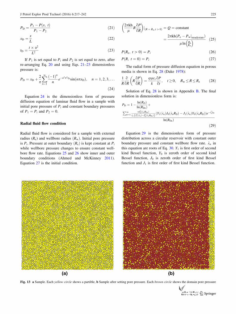
Fig. 13 a Sample. Each yellow circle shows a partible, b Sample after setting pore pressure. Each brown circle shows the domain pore pressure


123

Y1 knð ÞJ0 knRDeð Þ � J1 knð ÞY0 knRDeð Þ ¼ 0 ð30Þ

Knowing RDe, Eq. 30 can be solved to get the values of

kn. There are infinite numbers of kn that will satisfy this

equation and they are called eigenvalues of this equation.

Dimensionless parameters in Eq. 29 are defined as:

RD ¼ R

Rw

ð31Þ

tD ¼ kt

ulcR2w

ð32Þ

PD RD; tDð Þ ¼ Pi � P

Pi � Pwj steadystateð Þð33Þ

RD is dimensionless radius, tD is dimensionless time and

PD is dimensionless pressure.

Comparison of numerical and analytical models

Linear fluid flow with constant boundary pressures

Figure 13 shows a sample before setting the pore pressure

(a) and the same sample with pore pressure being set (b).

Right hand side of the sample in (b) has no pore pressure as

its pore pressure is set equal to zero and will be kept at zero

during fluid flow. The left hand side pressure will be kept

Fig. 14 Simulation results at four different times a t = 67 Seconds, b t = 267 Second, c t = 667 Seconds and d t = 15,067 Second


123

constant at initial pressure. Sample length is 14 meter, its

height is 14 meter and its width which is an out of plane

dimension is equal to one meter. The sample length

between the left boundary and the right boundary is 13.5

meters. Brown circles in Fig. 13b represent domain

pressure.

Figure 14 shows the simulation results at four different

times. Each point shows the pressure of a domain. Vertical

axis shows pressure in Mega Pascal (MPa) and horizontal

axes show the x and y position of the domain. The pressure

at left hand side is kept constant at initial pressure and

pressure at right hand side is kept constant at zero. At the

beginning of simulation, flow rate on the left hand side is

zero as pressure reduction wave has not reached it and the

flow rate on the right hand side is 1:101 � 10�3 m3=s.

The flow rate quickly drops on the right hand side as the

pressure on the right hand side start to fall down. As soon

as the pressure reduction wave reaches the left hand side,

the flow rate on left hand side start to increase. Flow rate

keeps increasing on left and falling on right until steady-

state flow rate is established. At steady-state condition,

flow rate on both sides is equal to 1:365 � 10�5 m3=s.

Figure 15 shows pressure distribution across sample with

each point representing the pressure of its domain. At

t ¼ 15067 s, a steady state flow regime is established.

To make sure that simulation results are correct, they are

compared against analytical results. To do so, data in

Fig. 15 are converted to dimensionless form by using

Eqs. 21–23.

The permeability of the simulated sample can be

obtained by using Darcy equation for linear flow in steady-

state condition as given by Eq. 34.

q ¼ 0:001127kAðP1 � P2ÞlL

ð34Þ

By inserting the values of different parameters from

Table 1 into Eq. 34, permeability is found to be

2:67 � 103 md. To confirm that this is the correct value,

another simulation has been conducted with different initial

pressure of 8:00 MPa. Steady state flow rate was

2:18 � 10�5 m3=s. Rest of the parameters were kept

constant. By inserting new values for initial pressure and

flow rate, permeability is calculated to be 2:67 � 103 md,

which is same as the value calculated before.

Dimensionless times and position are also inserted in

Eq. 24 to compare simulated versus analytical results.

Equation 35 is the dimensionless time in field units.

Table 2 shows simulation time in seconds and day and

calculated dimensionless time.

tD ¼ 0:006336kt

ulctL2ð35Þ

The units for different parameters are:

k: md, t: day, l: cp, c t: psi-1, L: ft.

Figure 16 shows results of simulation in dimensionless

form versus analytical results. It shows that data from

simulation match very well with analytical results and

validates the model for linear fluid flow.

Radial fluid flow

Radial fluid flow is simulated for a reservoir with constant

external boundary pressure and constant wellbore flow rate.

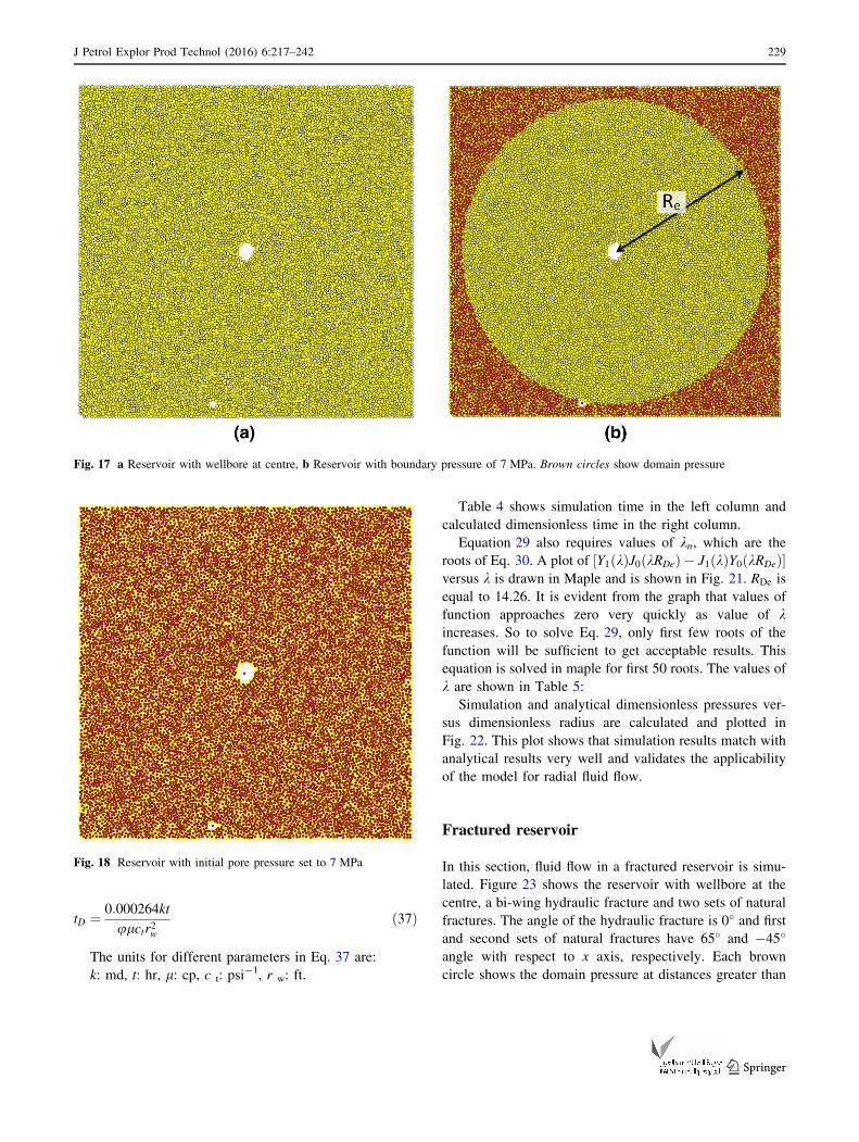
Figure 17a shows the reservoir with wellbore in the centre.

Fig. 15 Simulation results.

Pressure of domains against

linear distance from left hand

side of sample at different

times. As time increases,

domain pressures decrease until

a steady state condition is

established


123

Figure 17b shows the reservoir with boundary pressure set.

Pressure at distances more than external radius Re is con-

stant. Wellbore radius is Rw and height of the reservoir

which is out of plane dimension is equal to one. Each

brown circle represents pore pressure of a domain which is

kept constant at 7 MPa at distances greater than external

radius.

Figure 18 shows the reservoir with initial pore pressure

set to 7 MPa. The initial and boundary pressure are equal.

Figure 19 shows simulation results within the external

radius of the reservoir. Before starting production from

wellbore, the pressure across the whole reservoir is same

and equal to Pi. As production starts with constant wellbore

flow rate, pressure starts to decrease near the wellbore. As

simulation continuous, the pressure reduction wave prop-

agates toward the outer boundary. Before pressure reduc-

tion arrives at outer boundary, flow rate at outer boundary

is zero. As soon as the pressure reduces near the outer

boundary, the flow rate starts to increase. Flow rate keeps

rising until steady-state condition is reached. At steady-

state condition, outer boundary flow rate is equal to well-

bore flow rate.

Table 3 shows simulation parameters:

At steady state condition, wellbore pressure becomes

constant and equal to 3:49 � 106 Pa and is used to

determine the permeability of the reservoir. Steady state

radial flow in field units is:

Qjsteadystate ¼0:00708kh ðPe � PwÞ

l ln ðRe

RwÞ

ð36Þ

The units for different parameters are:

k: md, P: psia, l: cp, h: ft, R: ft.

Using Eq. 36, permeability is found to be equal to

2:44 � 103 md.

Figure 20 shows simulation results of pressure versus

radius. Vertical axis shows pressure in Pa and horizontal

axis shows radius in meters. Each point shows the pressure

of its domain versus the radial distance of the domain with

respect to wellbore centre. The figure shows that pressure

at outer boundary is kept constant while wellbore pressure

keeps reducing until steady state is reached. To make sure

that simulated results are correct, they are compared

against analytical results. To do so, Eq. 29 is used to find

the dimensionless pressure versus dimensionless radius. In

this equation, dimensionless time is required which is

calculated by Eq. 37:

Table 1 Parameters of simulation at steady state condition

Parameter Metric system Imperial system

q 1.37E-05 m3=s 7.42E?00 bbl/day

P1 5.00E?06 Pa 7.25E?02 psia

P2 0 Pa 0.00E?00 psia

A 14 m2 150:69 ft2

l 1 Pa:Sec 1000 cp

L 13.5 m 42:29 ft

c 1.00E-09 Pa�1 6.09E-06 psia�1

U 0:2 – 0:2 –

Table 2 Simulation time (t) and dimensionless time (tD)

t (seconds) t (day) tD

67 0.00078 0.00484

267 0.00309 0.01931

667 0.00772 0.04823

1467 0.01698 0.10608

3067 0.03550 0.22178

15067 0.17439 1.08951

Fig. 16 Simulated versus

analytical results. Vertical axis

shows dimensionless pressure

and horizontal axis shows

dimensionless position. On each

curve, coloured dots are

simulation results and black

dots are analytical results


123

tD ¼ 0:000264kt

ulctr2wð37Þ

The units for different parameters in Eq. 37 are:

k: md, t: hr, l: cp, c t: psi-1, r w: ft.

Table 4 shows simulation time in the left column and

calculated dimensionless time in the right column.

Equation 29 also requires values of kn, which are the

roots of Eq. 30. A plot of ½Y1 kð ÞJ0 kRDeð Þ � J1 kð ÞY0 kRDeð Þ�versus k is drawn in Maple and is shown in Fig. 21. RDe is

equal to 14.26. It is evident from the graph that values of

function approaches zero very quickly as value of kincreases. So to solve Eq. 29, only first few roots of the

function will be sufficient to get acceptable results. This

equation is solved in maple for first 50 roots. The values of

k are shown in Table 5:

Simulation and analytical dimensionless pressures ver-

sus dimensionless radius are calculated and plotted in

Fig. 22. This plot shows that simulation results match with

analytical results very well and validates the applicability

of the model for radial fluid flow.

Fractured reservoir

In this section, fluid flow in a fractured reservoir is simu-

lated. Figure 23 shows the reservoir with wellbore at the

centre, a bi-wing hydraulic fracture and two sets of natural

fractures. The angle of the hydraulic fracture is 0� and first

and second sets of natural fractures have 65� and �45�

angle with respect to x axis, respectively. Each brown

circle shows the domain pressure at distances greater than

Fig. 17 a Reservoir with wellbore at centre, b Reservoir with boundary pressure of 7 MPa. Brown circles show domain pressure

Fig. 18 Reservoir with initial pore pressure set to 7 MPa


123

external radius of the reservoir. Pore pressure of the

reservoir is not shown in this picture, but its initial value is

same as the boundary pressure and equal to 7 MPa.

Boundary pressure is kept constant and reservoir pore

pressure is allowed to drop to keep a constant wellbore

flow rate at 2 � 10�10 m3=s. Permeability of rock matrix

is 0:458 md and fracture permeability is 2:67 � 103 md.

Figure 24 shows two-dimensional view of pressure

distribution in the reservoir at six different times. In this

figure, it can be seen that pressure in the fractures drops at a

faster rate with respect to rock matrix pressure. Figure 25

shows a three-dimensional view of the pressure distribution

at time 38287:82 s. Because all the fractures have a T-

shaped connection at intersection with other fractures, their

pressure shows a V-shaped plot and the pressure data of

corresponding fracture can be identified easily.

Figure 26 shows three-dimensional view of the pressure

distribution at six different times. In Fig. 26a and b, only

pressure drop in hydraulic fracture can be seen. As the

pressure reduction wave arrives at the intersection of

hydraulic fracture and first set of natural fracture, pressure

start to drop in natural fracture and this can be seen in

Fig. 26c. Figure 26d shows the start of pressure drop in

second set natural fractures. The permeability of fractures

is adjusted by adjusting the aperture of the pipes that fall on

the position of the fracture. For simplicity of observing the

clear plot of pressure data in fractures, all fractures per-

meability was set to be same. But to account for the per-

meability difference between different sets of natural

Fig. 19 Simulation results at four different times a t = 120.03 Seconds, b t = 420.03, c t = 1420.03 and d t = 24,086.70 s

Table 3 Parameters of Simulation

Parameter Metric system Imperial system

q 2.00E-05 m3=s 7.42E?00 bbl=day

Pi 7.00E?06 Pa 1.02E?03 psia

Pe 7.00E?06 Pa 1.02E?03 psia

Pwjsteadystate 3.49E?06 Pa 5.06E?02 psia

rw 9.64E-01 m 3:16 ft

re 1.38E?01 m 45:11 ft

l 1 Pa:Sec 1000 cp

h 1 m 3:28 ft

c 1.00E-09 Pa�1 6.90E-06 psia�1

U 0:2 – 0:2 –


123

fractures as well as hydraulic fracture, the pipe apertures

can be adjusted.

This section showed how easily this model was modified

from simple circular reservoir to a hydraulically and nat-

urally fractured reservoir.

Potential application of the model

As stated earlier in introduction, fluid flow through porous

media has been the subject of interest in many fields of

study. The proposed model is expected to be considered in

areas associated with fluid flow through complex hetero-

geneous porous media subjected to anisotropic stress sys-

tem. The model is also expected to be used to study many

issues related to fluid production from, and injection into

porous media with complex situations, especially in case of

naturally fractured media, and hydraulic fractures inter-

Fig. 20 Simulation results of

Pressure vs. Radius

Table 4 Simulation time (t) and dimensionless time (tD)

t (seconds) tD

120.03 1.67

420.03 5.84

1420.03 19.75

2753.36 38.29

24,086.70 334.97

Table 5 Values of first 50 kn

n kn n kn N kn n kn n kn

1 0.170 11 2.499 21 4.863 31 7.230 41 9.598

2 0.395 12 2.735 22 5.099 32 7.467 42 9.835

3 0.624 13 2.971 23 5.336 33 7.704 43 10.072

4 0.855 14 3.207 24 5.573 34 7.941 44 10.309

5 1.088 15 3.444 25 5.810 35 8.177 45 10.546

6 1.322 16 3.680 26 6.046 36 8.414 46 10.783

7 1.557 17 3.916 27 6.283 37 8.651 47 11.020

8 1.792 18 4.153 28 6.520 38 8.888 48 11.256

9 2.027 19 4.390 29 6.757 39 9.125 49 11.493

10 2.263 20 4.626 30 6.993 40 9.362 50 11.730

Fig. 21 ½Y1 kð ÞJ0 kRDeð Þ � J1 kð ÞY0 kRDeð Þ� vs. k. The function approaches Zero very quickly as the value of k increases


123

Fig. 22 Simulated

dimensionless pressure and

Analytical dimensionless

pressure vs. dimensionless

radius

Fig. 23 Reservoir with

wellbore at centre, a bi-wing

hydraulic fracture and two sets

of natural fractures. Brown

circles show the reservoir

pressure at distances greater

than external radius


123

Fig. 24 Two dimensional view

of reservoir pressure at different

times. Each circle shows its

domain pressure. a 207.67 s,

b 825.19 s, c 2266.46 s,

d 5354.02 s, e 17,704.28 s and

f 38,287.82 s


123

acted with natural fractures in anisotropic stress system.

However, below are some of examples where the model

can potentially be used for simulation study:

1. Oil and gas flow in oil and gas reservoirs.

2. Injection of water or surfactants into oil and gas

reservoirs.

3. Both the injection and production simulation in oil and

gas reservoirs.

4. Single stage as well as multi stage hydraulic fracturing

of the oil and gas reservoirs such as shale gas

reservoirs.

5. Water flow in mines both in rock matrix as well as in

joints, faults and fractures for the application in mining

industry.

6. Water flow underground in soil to be used by civil

engineers for simulating water flow into tunnels.

7. Water movement in soil to be used by agricultural

engineers to simulate the rate of hydration, dehydra-

tion or draining of soil.

Conclusion

Deriving analytical expressions to describe fluid flow in

porous medium is a complex task. This is because for any

change in the reservoir geometry or any change in the

condition of fluid flow (e.g., transient, late transient, semi-

steady state or steady state) a new analytic expression

needs to be developed. In this view, a DEM based

numerical model is proposed to analyse the fluid flow

through reservoir’s porous media with complex character-

istics, especially in the case of existence of natural frac-

tures, hydraulic fractures and interaction of hydraulic and

natural fractures for any condition of fluid flow.

Proposed model is used to simulate and analyse some of

these field representative cases as an example case studies.

Both simple and complex cases are considered in this

study. The simple case is used to validate the accuracy of

the model. The DEM model that was used in this study is

observed to be independent of reservoir geometry as well

as the condition of fluid flow since it was shown that it

worked for both linear and radial flow without modifica-

tion. The simulation results are found to be in good

agreement with analytical results. It is also demonstrated

that the model can potentially be used as a powerful

numerical simulation tool to handle both simple and

complex reservoir conditions such as complex formations

with irregular shapes, and complex set of discontinuity and

fluid flow regime.

Acknowledgments I would like to express my appreciation to the

Australian and Western Australian Governments and the North West

Shelf Joint Venture Partners, as well as the Western Australian

Energy Research Alliance (WA:ERA) for their financial support to

undertake my research toward completion of my PHD.

Fig. 25 Three-dimensional view of reservoir pressure at time t = 38,287.82 s. Pressure in fractures is dropped at a fast rate


123

Open Access This article is distributed under the terms of the Crea-

tive Commons Attribution 4.0 International License (http://cre-

ativecommons.org/licenses/by/4.0/), which permits unrestricted use,

distribution, and reproduction in any medium, provided you give

appropriate credit to the original author(s) and the source, provide a link

to the Creative Commons license, and indicate if changes were made.

Appendix A

Derivation of analytical solution of linear fluid flow

in porous media

One dimensional fluid flow is considered in a sample with

dimensions of L � H �W . Initial pore pressure of the

sample is set equal to Pi. Boundaries have constant pres-

sure. Pressure at one end of the sample is P1 and on the

other end is P2. Equation 38 shows the initial condition.

Equations 39 and 40 show boundary conditions:

P x; t ¼ 0ð Þ ¼ Pi ¼ f xð Þ ð38ÞP x ¼ 0; t[ 0ð Þ ¼ P1 ð39ÞP x ¼ L; t[ 0ð Þ ¼ P2 ð40Þ

Equation 41 shows the linear form of pressure diffusion

equation in porous media (Donnez 2012):

oP

ot¼ a2

o2P

ox2; t� 0; 0� x� L ð41Þ

Fig. 26 Three-dimensional view of reservoir pressure at different times. Each circle shows its domain pressure. a 207.67 s, b 825.19 s,

c 2266.46 s, d 5354.02 s, e 17,704.28 s and f 38,287.82 s. Pressure in fractures dropped at quicker rate with respect to pressure in the rock matrix


123

a2 is called hydraulic diffusivity and is equal to fluid

mobility divided by fluid storability (Donnez 2012):

a2 ¼ k

ulctð42Þ

Equation 41 can be solved by separation of variables to get

an expression for pressure function that its variables are time

and location. Equation 41 can be solved easily for

homogenous boundary condition, i.e., boundary condition

values set to zero. But in this situation one or both of boundary

values can be a pressure above zero. To overcome this

problem and convert it to a homogenous boundary condition

equation, the pressure function can be assumed to be

composed of two parts of one being time-independent and

the other part being timedependent (Gonzalez-Velasco1996):

P x; tð Þ ¼ v xð Þ þ wðx; tÞ ð43Þ

In Eq. 43, vðxÞ is the steady state pressure equation that

is independent of time and aids to change the boundary

conditions of the problem to homogenous boundary

conditions. wðx; tÞ is the transient part of pressure

function and its value will change with respect to time.

Because vðxÞ is part of the pressure function equation, it

should satisfy the diffusivity equation as well. vðxÞ is

independent of time and its derivative with respect to time

is zero as shown in Eq. 44:

ov

ot¼ 0 ð44Þ

Replacing Pðx; tÞ by vðxÞ in Eq. 41 and using Eq. 44

gives:

a2o2v

ox2¼ 0 ð45Þ

The solution of Eq. 45 is:

v xð Þ ¼ c1xþ c2

Rewriting the boundary conditions for vðxÞ;P 0; tð Þ ¼v 0ð Þ ¼ P1 and P L; tð Þ ¼ v Lð Þ ¼ P2. Values of c1 and c2can be determined by these two boundary values

(Gonzalez-Velasco 1996):

v 0ð Þ ¼ P1 ¼ c1 � 0þ c2 ¼ c2

v Lð Þ ¼ P2 ¼ c1 � Lþ c2 ¼ c1

� Lþ P1 ! c1 ¼P2 � P1

L

v xð Þ ¼ P2 � P1

Lx þ P1

ð46Þ

Steady state part of the pressure equation is determined.

The next step is to find the transient part of the pressure

equation. The boundary values for the transient part are

calculated as follows (Gonzalez-Velasco 1996):

P 0; tð Þ ¼ P1 ¼ v 0ð Þ þ w 0; tð Þ ! w 0; tð Þ ¼ P1

� v 0ð Þ ¼ 0 ! w 0; tð Þ ¼ 0

w x ¼ 0; t [ 0ð Þ ¼ 0

ð47Þ

P L; tð Þ ¼ P2 ¼ v Lð Þ þ w L; tð Þ ! w L; tð Þ ¼ P2

� v Lð Þ ¼ 0 ! w L; tð Þ ¼ 0

w x ¼ L; t[ 0ð Þ ¼ 0

ð48Þ

P x; 0ð Þ ¼ f xð Þ ¼ Pi ¼ v xð Þ þ w x; 0ð Þ ! w x; 0ð Þ

¼ f xð Þ � v xð Þ ¼ Pi � ðP1 þP2 � P1

LxÞ

w x; t ¼ 0ð Þ ¼ Pi � ðP1 þP2 � P1

LxÞ

ð49Þ

As w x; tð Þ is also part of the pressure equation, so it

should satisfy the partial differential pressure diffusivity

equation:

ow

ot¼ a2

o2w

ox2; 0� x� L; t� 0 ð50Þ

This equation can be solved by the method of separation

of variables. If w x; tð Þ is denoted as a multiplication of two

functions that one of them is only dependent on x and the

other is dependent on time then (Schroder 2009):

w x; tð Þ ¼ XðxÞ � TðtÞ ð51Þ

Partial derivatives of w x; tð Þ with respect to time (t) and

position (x) are:

o2w

ox2¼ TðtÞ o

2X

ox2ð52Þ

ow

ot¼ XðxÞ oT

otð53Þ

Substitution of Eqs. 52 and 53 into Eq. 50 gives:

XoT

ot¼ a2T

o2X

ox2ð54Þ

If either of XðxÞ or TðtÞ is zero, then the solution of

wðx; tÞ is the trivial solution of w x; tð Þ ¼ 0. So both of these

functions are different from zero and both sides of Eq. 54

can be divided by X xð ÞTðtÞ to give:

1

a2ToT

ot¼ 1

X

o2X

ox2ð55Þ

Sides of Eq. 55 are independent of each other. The left

hand side is a function of time (t) and the right hand side is

a function of position (x). So in order for equation to hold

for any t and x, both sides should be equal to a constant

(Schroder 2009). If sides are equated to -k (-k can be any

positive or negative number but the negative sign makes

calculations simpler) it will result in:

X00 þ kX ¼ 0 ð56Þ


123

And,

T0 þ a2kT ¼ 0 ð57Þ

So Wðx; tÞ decomposed to a homogenous second order

ordinary differential equation for XðxÞ and a homogenous

first order ordinary differential equation for TðtÞ. Solvingfor boundary conditions:

w 0; tð Þ ¼ 0 ! X 0ð ÞT tð Þ ¼ 0 ! X 0ð Þ ¼ 0 or T tð Þ ¼ 0

w L; tð Þ ¼ 0 ! X Lð ÞT tð Þ ¼ 0 ! X Lð Þ ¼ 0 or T tð Þ ¼ 0

T tð Þ ¼ 0 will make both of the conditions to satisfy but it

also causes w x; tð Þ equation to be zero which is a trivial

solution and not the desired solution. Therefore;

X x ¼ 0ð Þ ¼ 0 ð58ÞX x ¼ Lð Þ ¼ 0 ð59Þ

To solve Eq. 56 there are three options for k:

Option 1: k < 0

Option 2: k = 0

Option 3: k > 0

Three options will be considered individually to decide

which option will give the correct answer:

Option 1: k < 0

k ¼ �d2 so the characteristic equation is (Kreyszig

2010): r2 � d2 ¼ 0 and roots are r ¼ d.This gives the general solution as (Kreyszig 2010):

X xð Þ ¼ D1edx þ D2e

�dx ð60Þ

Putting the first boundary condition from Eq. 58 into Eq.

60 gives:

X 0ð Þ ¼ 0 ¼ D1 þ D2 ! D1 ¼ �D2 ð61Þ

Putting the second boundary condition from Eq. 59 into

Eq. 60 gives:

X Lð Þ ¼ 0 ¼ D1edL þ D2e

�dL ¼ D1ðedL þ e�dLÞ ð62Þ

ðedL þ e�dLÞ 6¼ 0 and for Eq. 62 to hold, D1 should be zero

which causes D2 to be zero as well. This will result in

X xð Þ ¼ 0 which in turn causes w x; tð Þ ¼ 0 which is a trivial

solution. So this means that option 1 is not valid and kcannot be a negative value.

Option 2: k = 0

This option will result in Eq. 63 for X xð Þ:X xð Þ ¼ D1 þ D2x ð63Þ

Applying the first boundary condition will results in:

X 0ð Þ ¼ 0 ¼ D1 ! D1 ¼ 0

And applying the second boundary condition will result

in:

X Lð Þ ¼ 0 ¼ D1 þ D2L ¼ D2L ! D2 ¼ 0

This will result in X xð Þ ¼ 0 which in turn causes

w x; tð Þ ¼ 0 which is a trivial solution. So this means that

option 2 is not valid and k cannot be zero and only option 3

is left.

Option 3: k > 0

k ¼ d2 so the characteristic equation is (Kreyszig

2010): r2 ? d2 = 0 and roots are r ¼ di. So based on

the roots of the characteristic equation the general solution

is (Kreyszig 2010):

X xð Þ ¼ D1 cosðdxÞ þ D2 sinðdxÞ ð64Þ

By imposing the boundary conditions:

X 0ð Þ ¼ 0 ¼ D1 cos 0ð Þ þ D2 sin 0ð Þ ¼ D1 ! D1 ¼ 0

X Lð Þ ¼ 0 ¼ D1 cos dLð Þ þ D2 sin dLð Þ ¼ D2 sin dLð Þ

For D2 sin dLð Þ ¼ 0 to be valid; either D2 ¼ 0 or

sin dLð Þ ¼ 0. If D2 ¼ 0, will result in X xð Þ ¼ 0 which in

turn causes w x; tð Þ ¼ 0 which is a trivial solution. So this

means that sin dLð Þ ¼ 0 which implies that

dL ¼ p; 2p; 3p; . . .; np. Solving for d will give:

d ¼ pL; 2pL; . . .; np

L.

So based on the above three options being analysed, the

value of k should be greater than zero. The values of k that

satisfy Eq. 64 are eigenvalues of this equation and are:

k ¼ d2 ¼ n2p2

L2; n ¼ 1; 2; 3; . . . ð65Þ

For each of eigenvalues there will be an eigen function.

The nth eigen function is:

XnðxÞ ¼ sinnpxL

; n ¼ 1; 2; 3; . . . ð66Þ

Inserting the value of k from Eq. 65 into Eq. 57 will

give:

T 0 þ a2n2p2

L2T ¼ 0 ð67Þ

Solving Eq. 67 will give T(t) for nth eigenvalue:

Tn tð Þ ¼ Cne�a2n2p2

L2t; n ¼ 1; 2; 3; . . . ð68Þ

The nth eigen function for w x; tð Þ is the product of Eqs.

66 and 68:


123

wn x; tð Þ ¼ Xn xð ÞTn tð Þ ¼ Cne�a2n2p2

L2tsin

npxL

;

n ¼ 1; 2; 3; . . .ð69Þ

The summation of all solutions for different eigenvalues

is also a solution of w x; tð Þ. As a result w x; tð Þ can be shownas:

w x; tð Þ ¼X1

n¼1

XnðxÞTn tð Þ ¼X1

n¼1

Cne�a2n2p2

L2tsin

npxL

;

n ¼ 1; 2; 3; . . .

ð70Þ

Applying the initial condition of w x; 0ð Þ ¼ f xð Þ � v xð Þgives:

w x; 0ð Þ ¼X1

n¼1

Cn sinnpxL

¼ f xð Þ � v xð Þ; n ¼ 1; 2; 3; . . .

ð71Þ

Equation 71 is ‘‘sine’’ Fourier series (Kreyszig 2010).

The coefficients Cn which are the ‘‘sine’’ Fourier

coefficients are:

Cn ¼2

L

ZL

0

f xð Þ � v xð Þð Þ sin npxL

dx

¼ 2

L

ZL

0

Pi � ðP1 þP2 � P1

LxÞ

� �

sinnpxL

dx

¼ 2

L

ZL

0

Pi � P1ð Þ sin npxL

dxþ 2

L

ZL

0

P1 � P2

Lx

� �

sinnpxL

dx

¼ 2

L

�L

npcos

npxL

� �Pi � P1ð Þ

��L

0þ 2

L2P1 � P2ð Þ

ZL

0

x� sinnpxL

dx

¼ 2 Pi � P1ð Þ 1� cos npð Þð Þnp

þ 2

L2P1 � P2ð Þ � L2 � sin npð Þð Þ þ cos npð Þ � np

n2p2

� �

;

n ¼ 1; 2; 3; . . .

Cn ¼2ðPi � P1Þð1� ð�1ÞnÞ

npþ 2 P2 � P1ð Þ ð�1Þn

np

� �

; n

¼ 1; 2; 3; . . .

ð72Þ

Inserting Eq. 72 into Eq. 70:

w x; tð Þ ¼X1

n¼1

2ðPi � P1Þð1� ð�1ÞnÞnp

�

þ 2 P2 � P1ð Þ ð�1Þn

np

� ��

e�a2n2p2

L2tsin

npxL

; n ¼ 1; 2; 3; . . .

ð73Þ

Inserting Eqs. 46 and 73 in Eq. 43 gives:

P x; tð Þ ¼ P1 þP2 � P1

Lx

� �

þX1

n¼1

ð2 Pi � P1ð Þ 1� �1ð Þnð Þnp

þ 2 P2 � P1ð Þ �1ð Þn

np

� �

Þe�a2n2p2

L2tsin

npxL

;

n ¼ 1; 2; 3; . . . ð74Þ

Appendix B

Derivation of analytical solution of radial fluid flow

in porous media in a finite circular reservoir

Radial fluid flow is considered for a sample with external

radius (Re) and wellbore radius ðRwÞ. Initial pore pressure

is Pi. Pressure at outer boundary ðReÞ is kept constant at Pi

while wellbore pressure changes to ensure constant well-

bore flow rate. Equations 75 and 76 show inner and outer

boundary conditions (Ahmed and McKinney 2011).

Equation 77 is the initial condition.

2pkhl

RoP

oR

� �

j R¼Rw; t[ 0ð Þ ¼ Q ¼ constant

¼2pkhðPe � PwjsteadystateÞ

llnðRe

RwÞ

ð75Þ

P Re; t[ 0ð Þ ¼ Pi ð76ÞP R; t ¼ 0ð Þ ¼ Pi ð77Þ

The radial form of pressure diffusion equation in porous

media is shown in Eq. 78 (Dake 1978):

1

R

o

oRRoP

oR

� �

¼ ulctk

oP

ot; t� 0; Rw �R�Re ð78Þ

To simplify (78) and boundary conditions, the following

dimensionless parameters are defined:

RD ¼ R

Rw

ð79Þ

tD ¼ kt

ulcR2w

ð80Þ

DPD ¼ 2pkhðPi � PÞlQ

ð81Þ

RD is dimensionless radius, tD is dimensionless time and

DPD is delta dimensionless pressure. Inserting Eqs. 79, 80

and 81 into Eq. 78, will simplify it to Eq. 82:

1

RD

o

oRD

RD

oDPD

oRD

� �

¼ oDPD

otD; tD � 0; 1�RD �RDe

ð82Þ

Boundary conditions and Initial condition will simplify to:


123

DPD RD ¼ 1; tDð Þ ¼ ln RDeð Þ;RD

oDPD

oRD

j RD¼1;tDð Þ ¼ �1

ð83ÞDPD RD ¼ RDe; tDð Þ ¼ 0 ð84ÞDPD RD; 0ð Þ ¼ 0 ð85Þ

Equation 82 can be solved in the same way as linear

form of the equation has been solved by assuming that the

equation is composed of two parts of steady state and

unsteady state.

DPD RD; tDð Þ ¼ S RDð Þ þ U RD; tDð Þ ð86Þ

S RDð Þ is the steady state part of the equation and

U RD; tDð Þ is the unsteady state part of the equation. Steady

state part of the equation should satisfy initial and

boundary conditions as well as pressure diffusion

equation. As the steady state solution is independent of

time, the right hand side of the diffusivity equation is equal

to zero.

1

RD

o

oRD

RD

oS RDð ÞoRD

� �

¼ 0; tD � 0; 1�RD �RDe

ð87ÞS RD ¼ 1ð Þ ¼ ln RDeð Þ ð88ÞS RD ¼ RDeð Þ ¼ 0 ð89Þ

Solving Eq. (87) gives:

S RDð Þ ¼ C1 ln RDð Þ þ C2 ð90Þ

Inserting boundary conditions from Eqs. (88) and (89)

into Eq. (87) results in C2 ¼ lnðRDeÞ and C1 ¼ �1 and

therefore;

S RDð Þ ¼ � lnRD

RDe

� �

ð91Þ

The steady state part of the dimensionless pressure

equation is solved. The unsteady state part needs to be

solved. But first its boundary and initial conditions need to

be determined. Using the second part of Eq. 83:

RD

oDPD

oRD

j RD¼1;tDð Þ ¼ �1 ! RD

o Sþ Uð ÞoRD

j RD¼1;tDð Þ

¼ RD � 1

RD

þ o Uð ÞoRD

j RD¼1;tDð Þ

� �

¼ �1

! RD

o Uð ÞoRD

j RD¼1;tDð Þ ¼ 0

Therefore;

RD

o Uð ÞoRD

j RD¼1;tDð Þ ¼ 0 ð92Þ

Inserting Eqs. 84 and 89 into Eq. 86, gives:

DPD RDe; tDð Þ ¼ 0 ¼ S RDeð Þ þ U RDe; tDð Þ¼ 0þ U RDe; tDð Þ ! U RDe; tDð Þ ¼ 0

U RDe; tDð Þ ¼ 0 ð93Þ

Inserting Eqs. 85 and 91 into Eq. 86, gives:

DPD RD; 0ð Þ ¼ 0 ¼ S RDð Þ þ U RD; 0ð Þ

¼ � lnRD

RDe

� �

þ U RD; 0ð Þ !

U RD; 0ð Þ ¼ lnRD

RDe

� �

U RD; 0ð Þ ¼ lnRD

RDe

� �

ð94Þ

Equations 92 and 93 are the boundary conditions for the

unsteady state equation and Eq. 94 is its initial condition.

Same as what has been done to solve the transient part

of the pressure equation for linear flow, in here the concept

of separation of variables is used to solve U RD; tDð Þ.U RD; tDð Þ can be shown to be a multiplication of two

functions with one being dependent on time and the other

dependent on space or radius.

UD RD; tDð Þ ¼ TðtDÞX RDð Þ ð95Þ

By applying boundary conditions from Eqs. 92 and 93 to

Eq. 95:

U RD ¼ 1; tDð Þ ¼ 0 ¼ T tDð ÞX 1ð Þ ! T tDð Þ ¼ 0 orX 1ð Þ¼ 0

U RDe; tDð Þ ¼ 0 ¼ T tDð ÞX RDeð Þ ! T tDð Þ ¼ 0 orX RDeð Þ¼ 0

If T tDð Þ ¼ 0 then U RD; tDð Þ ¼ 0; which is not of

interest. Therefore;

X RD ¼ 1ð Þ ¼ 0 ð96ÞX RDeð Þ ¼ 0 ð97Þ

As UD RD; tDð Þ is part of dimensionless pressure

equation, it should satisfy the dimensionless partial

differential equation:

1

RD

o

oRD

RD

oUD

oRD

� �

¼ oUD

otD; tD � 0; 1�RD �RDe

ð98Þ

Partial derivatives of UD RD; tDð Þ with respect to time

and space are:

1

RD

o

oRD

RD

oUD

oRD

� �

¼ TðtDÞ1

RD

d

dRD

RD

dX

dRD

� �

ð99Þ

oUD

otD¼ X RDð Þ dT

dtDð100Þ


123

Substitution of Eqs. 99 and 100 into Eq. 98 gives:

T tDð Þ 1

RD

d

dRD

RD

dX

dRD

� �

¼ X RDð Þ dTdtD

ð101Þ

If either of T tDð Þ or X RDð Þ is equal to zero then

UD RD; tDð Þ will be equal to zero which is not of interest.

Therefore, both T tDð Þ and X RDð Þ are different from zero. If

both sides of Eq. 101 are divided by T tDð Þ � X RDð Þ, itgives:

1

RDX RDð Þd

dRD

RD

dX

dRD

� �

¼ 1

T tDð ÞdT

dtDð102Þ

Sides of Eq. 102 are independent of each other. The left

hand side is dependent on location or radius and the right

hand side is dependent on time. In order for Eq. 102 to hold

for any time and location, both sides should be equal to a

constant. Sides can be equated to � . Same arguments can

be made about the sign of � as before for the linear

pressure diffusion equation. In here, it can be shown that �

should be a negative value �k2 for equation to hold. So

equating both sides to �k2 will give:

1

T tDð ÞdT

dtD¼ �k2 ð103Þ

Solving Eq. 103 gives:

TðtDÞ ¼ Ae�k2tD ð104Þ

In Eq. 104, A is a constant.

1

RDX RDð Þd

dRD

RD

dX

dRD

� �

¼ �k2 ! d2X

dR2D

þ 1

RD

dX

dRD

þ k2X

¼ 0

d2X

dR2D

þ 1

RD

dX

dRD

þ k2X ¼ 0 ð105Þ

Equation 105 can be solved in maple as shown below:

dslove diff ðdiffðX Rð Þ;RÞ;RÞ þ 1

R� diffðX Rð Þ;RÞ þ k2 X Rð Þ ¼ 0

� �

X Rð Þ ¼ C1 Besse1J 0; kRð Þ þ C2 Besse1Y 0; kRð Þ

So the answer to Eq. 105 is:

X RDð Þ ¼ C1J0 kRDð Þ þ C2Y0 kRDð Þ ð106Þ

J0 in Eq. 106 is first kind of Bessel function of order

zero and Y0 is second kind of Bessel function of order zero

(Polyanin and Manzhirov 2008). To determine constants of

the equation, boundary conditions form Eqs. 92 and 93 are

applied to Eq. 106:

RD

o Uð ÞoRD

j RD¼1;tDð Þ ¼ 0

¼ RD

o C1J0 kRDð Þ þ C2Y0 kRDð Þð ÞoRD

j RD¼1;tDð Þ

! RD �C1kJ1 kRDð Þ � C2kY1 kRDð Þð Þj RD¼1;tDð Þ

¼ 0 ! C1J1 kð Þ þ C2Y1 kð Þ ¼ 0

C1J1 kð Þ þ C2Y1 kð Þ ¼ 0 ð107ÞC1J0 kRDeð Þ þ C2Y0 kRDeð Þ ¼ 0 ð108Þ

Solving Eq. 107 for C2 gives:

C2 ¼ �C1J1 kð ÞY1 kð Þ

Replacing above equation in Eq. 108 gives:

C1J0 kRDeð Þ � C1J1 kð ÞY1 kð Þ Y0 kRDeð Þ ¼ 0

! C1ðJ0 kRDeð ÞY1 kð Þ � J1 kð ÞY0 kRDeð ÞÞ ¼ 0

! C1 ¼ 0orJ0 kRDeð ÞY0 kð Þ � J0 kð ÞY0 kRDeð Þ ¼ 0

If C1 ¼ 0, it implies that C2 ¼ 0 and as a result X Rð Þ ¼0 which is not of interest. Therefore;

Y1 kð ÞJ0 kRDeð Þ � J1 kð ÞY0 kRDeð Þ ¼ 0 ð109Þ

Knowing RDe, Eq. 109 can be solved to get the value of

k. There are infinite numbers of k that will satisfy this

equation and they are called eigenvalues of this equation.

Eigenvalues are represented as kn. For every kn; there is a

C1n, C2n and as a result there is a Xn Rð Þ:

C2n ¼ �C1nJ1 knð ÞY1 knð Þ ð110Þ

Xn RDð Þ ¼ C1nJ0 knRDð Þ � C1nJ1 knð ÞY1 knð Þ Y0 knRDð Þ

¼ CnðY1 knð ÞJ0 knRDð Þ � J1 knð ÞY0 knRDð ÞÞ ð111Þ

As every Xn RDð Þ is a solution for Eq. 95, their

summation is also a solution for Eq. 95. Inserting Eq.

104 and 111 into Eq. 95 gives:

UD RD; tDð Þ ¼X1

n¼1

CnðY1 knð ÞJ0 knRDð Þ

� J1 knð ÞY0 knRDð Þe�k2ntD ð112Þ

Applying the initial condition from Eqs. 94 to 112 gives:

X1

n¼1

CnðY1 knð ÞJ0 knRDð Þ � J1 knð ÞY0 knRDð ÞÞ ¼ lnRD

RDe

� �

ð113Þ


123

Cn can be shown to be (Muskat 1982):

Cn ¼pJ20 knRDeð Þ

knðJ21 knð Þ � J20 knRDeð ÞÞ ð114Þ

Inserting Eq. 114 into Eq. 112 gives:

UD RD; tDð Þ ¼X1

n¼1

pJ20 knRDeð ÞknðJ21 knð Þ � J20 knRDeð ÞÞ ðY1 knð ÞJ0 knRDð Þ

� J1 knð ÞY0 knRDð ÞÞe�k2ntD

ð115Þ

Equation 115 is the final solution of the un-steady state

part of pressure equation. Inserting Eqs. 91 and 115 into

Eq. 86 gives the final solution to pressure equation (Muskat

1982):

DPD RD;tDð Þ¼�lnRD

RDe

� �

þX1

n¼1

pJ20 knRDeð ÞknðJ21 knð Þ�J20 knRDeð ÞÞðY1 knð ÞJ0 knRDð Þ

�J1 knð ÞY0 knRDð ÞÞe�k2ntD

ð116Þ

Dimensionless pressure is defined as:

PD RD; tDð Þ ¼ Pi � P

Pi � Pwj steadystateð Þð117Þ

Wellbore flow rate at any time is constant and is equal to

steady state flow rate. Steady state flow rate is:

Q ¼2pkhðPi � PwjsteadystateÞ

l ln Re

Rw

� � ð118Þ


DPD ¼ 2pkhðPi � PÞlQ

¼ 2pkhðPi � PÞl 2pkhðPi�Pwj steadystateÞ

l ln ReRwð Þ

¼ Pi � P

Pi � Pwj steadystateln RDeð Þ ¼ PD ln RDeð Þ

DPD ¼ PD lnðRDeÞ ð119Þ


PD lnðRDeÞ ¼ � lnRD

RDe

� �

þX1

n¼1

pJ20 knRDeð ÞknðJ21 knð Þ � J20 knRDeð ÞÞ ðY1 knð ÞJ0 knRDð Þ

� J1 knð ÞY0 knRDÞð Þe�k2ntD

! PD ¼ 1� lnðRDÞln RDeð Þ

þP1

n¼1

pJ20knRDeð Þ

knðJ21 knð Þ�J20knRDeð ÞÞ ðY1 knð ÞJ0 knRDð Þ � J1 knð ÞY0 knRDð ÞÞe�k2ntD

ln RDeð Þ

PD ¼ 1� ln RDð Þln RDeð Þþ

P1n¼1

pJ20knRDeð Þ

knðJ21 knð Þ�J20knRDeð ÞÞ ðY1 knð ÞJ0 knRDð Þ � J1 knð ÞY0 knRDð ÞÞe�k2ntD

ln RDeð Þð120Þ

Equation 120 is the dimensionless pressure distribution

across a circular finite reservoir with constant outer

boundary pressure and constant wellbore flow rate.

References

Ahmed T, McKinney P (2011) Advanced reservoir engineering.

Elsevier, Amsterdam

Cundall PA (1988) Formulation of a three-dimensional distinct

element model—Part I. A scheme to detect and represent

contacts in a system composed of many polyhedral blocks. Int J

Rock Mech Min Sci Geomech Abstr 25:107–116. doi:10.1016/

0148-9062(88)92293-0

Cundall PA, Hart RD (1992) Numerical modelling of discontinua.

Eng Comput Int J Comp Aided Eng Softw 9:13

Cundall PA, Strack ODL (1979) A discrete numerical model for

granular assemblies. Geotechnique 29:47–65. (citeulike-article-id:9245301)

Dake LP (1978) Fundamentals of reservoir engineering. Elsevier,

Amsterdam

Donnez P (2012) Essentials of Reservoir Engineering. vol 5, 2nd Edn.

Technip

Garde RJ (1997) Fluid Mechanics Through Problems. New Age

International

Gonzalez-Velasco EA (1996) Fourier analysis and boundary value

problems. Elsevier, Amsterdam

Hart R, Cundall PA, Lemos J (1988) Formulation of a three-

dimensional distinct element model—Part II. Mechanical calcu-

lations for motion and interaction of a system composed of many

polyhedral blocks International Journal of Rock Mechanics and

Mining Sciences & Geomechanics Abstracts 25:117–125.

doi:10.1016/0148-9062(88)92294-2

Huynh KDV (2014) Discrete Element Method (DEM). http://www.

ngi.no/no/Innholdsbokser/Referansjeprosjekter-LISTER-/

Referanser/Discrete-Element-Method-DEM/

Itasca (2008a) Particle Flow Code in 2 Dimensions vol Theory and

Background. Fourth edn. Itasca Consulting Group Inc.,

Itasca (2008b) Particle Flow Code in 2 Dimensions vol Verification

Problems and Example Applications. Fourth edn. Itasca Con-

sulting Group Inc.,

Jing L, Stephansson O (2007) Fundamentals of discrete element

methods for rock engineering: theory and applications: theory

and applications. Elsevier, Amsterdam

Kreyszig E (2010) Advanced engineering mathematics. Wiley, New

York

Morris J, Glenn L, Blair S (2003) The Distinct Element Method—

Application to Structures in Jointed Rock. In: Griebel M,

Schweitzer M (eds) Meshfree Methods for Partial Differential

Equations, vol 26. Lecture Notes in Computational Science and

Engineering. Springer, Berlin, Heidelberg, pp 291–306. doi:10.

1007/978-3-642-56103-0_20

Muskat M (1982) The flow of homogeneous fluids through porous

media. International Human Resources Development Corporation


123

http://dx.doi.org/10.1016/0148-9062(88)92293-0

http://dx.doi.org/10.1016/0148-9062(88)92293-0

http://dx.doi.org/10.1016/0148-9062(88)92294-2

http://www.ngi.no/no/Innholdsbokser/Referansjeprosjekter-LISTER-/Referanser/Discrete-Element-Method-DEM/



http://dx.doi.org/10.1007/978-3-642-56103-0_20

http://dx.doi.org/10.1007/978-3-642-56103-0_20

Polyanin AD, Manzhirov AV (2008) Handbook of Integral Equations,

2nd edn. Taylor & Francis, London

Schroder BSW (2009) A Workbook for Differential Equations.

Wiley, New York

Tavarez FA (2005) Discrete element method for modeling solid and

particulate materials:172

Zhao DX (2010) Imaging the mechanics of hydraulic fracturing in

naturally-fractured reservoirs using induced seismicity and

numerical modeling:285


123

fluid flow through porous media using distinct … paper - production engineering fluid ﬂow...

Documents