finite volume methods for fluid flow in porous media
TRANSCRIPT

Finite volume methods for fluidflow in porous media
Bachelor Thesis
Fabian Mönkeberg
Supervisor: Prof. Dr. Nils Henrik Risebro,Prof. Dr. Ralf Hiptmair
ETH Zürich,June 27, 2012

i
Acknowledgments
This thesis was done to receive the Bachelor of Science in Mathemetics.I first thank my supervisor Prof. Dr. Nils Henrik Risebro for motivating meand for his good advices. I also thank Prof. Dr. Ralf Hiptmair for his support.Finally, I thank Simon Laumer for all the corrections.

Contents
1 Introduction 1
2 Modeling fluid flow in porous media 32.1 Rock and fluid properties . . . . . . . . . . . . . . . . . . . . . . 42.2 Single-phase flow . . . . . . . . . . . . . . . . . . . . . . . . . . . 6
2.2.1 Single-phase flow in one dimension . . . . . . . . . . . . . 62.2.2 Single-phase flow in two and three dimensions . . . . . . . 72.2.3 Boundary conditions . . . . . . . . . . . . . . . . . . . . . 72.2.4 Special cases of single-phase flow . . . . . . . . . . . . . . 8
2.3 Two-phase flow . . . . . . . . . . . . . . . . . . . . . . . . . . . . 92.3.1 General solution . . . . . . . . . . . . . . . . . . . . . . . 92.3.2 Pressure equation . . . . . . . . . . . . . . . . . . . . . . 102.3.3 Pressure equation for incompressible immiscible flow . . . 112.3.4 Saturation equation . . . . . . . . . . . . . . . . . . . . . 112.3.5 Saturation equation for incompressible flow . . . . . . . . 12
2.4 Three-phase flow . . . . . . . . . . . . . . . . . . . . . . . . . . . 122.5 Multiphase and multicomponent flows . . . . . . . . . . . . . . . 13
2.5.1 Black-oil model . . . . . . . . . . . . . . . . . . . . . . . . 14
3 Elliptic pde’s 153.1 Setting and definitions . . . . . . . . . . . . . . . . . . . . . . . . 15
3.1.1 Weak derivative: . . . . . . . . . . . . . . . . . . . . . . . 163.1.2 Sobolev spaces: . . . . . . . . . . . . . . . . . . . . . . . . 16
3.2 Discretization of the elliptic problem/Galerkin approximation . . 17
4 Hyperbolic pde’s 194.1 Riemann problem . . . . . . . . . . . . . . . . . . . . . . . . . . . 204.2 Numerical methods for hyperbolic equations in 1-D . . . . . . . . 21
4.2.1 Finite difference schemes . . . . . . . . . . . . . . . . . . 214.3 Numerical methods for hyperbolic equations in 2-D . . . . . . . . 24
4.3.1 Splitting schemes . . . . . . . . . . . . . . . . . . . . . . . 244.3.2 Finite volume methods . . . . . . . . . . . . . . . . . . . . 24

CONTENTS iii
5 FVM in 2-D on triangulation 275.1 Mesh construction . . . . . . . . . . . . . . . . . . . . . . . . . . 275.2 Construction of the finite volume method . . . . . . . . . . . . . 325.3 Construction of a Galerkin approximation routine . . . . . . . . . 34
5.3.1 Element stiffness matrix . . . . . . . . . . . . . . . . . . . 355.3.2 Load vector . . . . . . . . . . . . . . . . . . . . . . . . . . 36
5.4 Simulation of flow in porous media . . . . . . . . . . . . . . . . . 36
6 Conclusion and further work 48

CONTENTS iv
Abstract
This thesis develops a routine to compute finite volume methods on triangulargrids for solving hyperbolic partial differential equations. The implementationin this thesis is based on the Engquist-Osher scheme, but it can be extended toany other finite volume method.In the second part, we test the implementation against a benchmark datasetfor reservoir simulation of the Society of Petroleum Engineers. This dataset isused to define an immiscible and incompressible two-phase flow in a rectangulardomain. We had to implement a fast elliptic solver, due the needed split in anelliptic and one hyperbolic equation.The focus of these thesis is the implementation, not the convergence theory.

CHAPTER 1. INTRODUCTION 1
Chapter 1
Introduction
The topic of this thesis is first the development of a program of a finite volumemethod on a triangular mesh. Second focus was its verification based on sim-ulations of flow in porous media. Nowadays, an approved method is the finitevolume method on a Cartesian grid. The advantage of a method on a Cartesiangrid is its simple handling, due to its nice structure. On the other hand, theadvantage of a method on a triangular mesh is a certain flexibility. Being moreprecise, there exist several simple strategies for local refinements. Examples ofsuch local refinements are shown in figure 1.1 and 1.2. In this figures ∗ denotesthe triangle that should be refined. Note that, in order to receiving a correcttriangulation, we can not just refine one single triangle. We have to guarantee,that the mesh is complete. Local refinements are used to guarantee convergence,without refining the whole grid.
Figure 1.1: local refinement of triangular grid, [6]
Figure 1.2: local refinement of triangular grid, [6]
An other approach, which can be used on triangular grids, is local grid align-
CHAPTER 1. INTRODUCTION 2
ment. There you align the triangles in the direction of the flux or parallelizethem according to the shock waves. A shock wave is a discontinuous wave. Thisapproach improves the accuracy, too. The disadvantage is exactly that thereare a lot of possibilities to build a triangulation, and so we have no fix topology.The aim is to find a method to get access to the informations of this topology(triangular elements, neighbors of triangles, size of triangles,...).

CHAPTER 2. MODELING FLUID FLOW IN POROUS MEDIA 3
Chapter 2
Modeling fluid flow inporous media
The interest in the behavior of fluid in porous media is not a recency. It startedin the early days of the oil production out of reservoirs deep under the surfaceof the earth. The main purpose in modeling fluid flow in porous media is tosimulate the flow of oil and water in the rock, to estimate and optimize the oiland gas production. Another application is the simulation of groundwater con-tamination. The existence of many depends on the subsistence of groundwater.Problems appear from leaking tanks of chemicals, oil pipelines, or fertilizers. Ingeneral, the whole pollution of the environment is problematic for the groundwater. The basic process is that we have clean groundwater as one medium andpolluted water, or even an toxic fluid as the second medium. To understand thespreading of the second medium and its consequences is the aim.The challenge is to model an interaction of different fluids in their phases (liq-uid, gaseous, solid) and the environment. Basically, this means to simulate fluidflow and mass transfer, while some external and internal forces, like gravity,capillary and viscous forces, affect.The mathematical model of this physical system is set by differential equationsand some special boundary conditions. To get these we use the fundamentalrules of conservation of mass, momentum and often we apply Darcy’s law (p.5)for each phase, instead of Newton’s second law. The first challenge is to get anaccurate prediction of the flow scenarios, this means to receive the propertiesof the different media and its interaction. Nowadays, their is an amount of newand reliable techniques for getting these informations. But handling this hugemass of data is the next difficult task. It is just impossible to run simulationswith all this information. This is because of the still limited computer resources.So a suitable approximation is the key concept to solve this task. For furtherinformations, this chapter is based on the books [10], [2], [11] and the article [5].

CHAPTER 2. MODELING FLUID FLOW IN POROUS MEDIA 4
2.1 Rock and fluid propertiesThe rock compressibility cr is a measure of how much the rock is compressibleand is defined by:
cr = 1φ
dφ
dp, (2.1)
where p is the overall reservoir pressure and φ, the porosity, is the void volumefraction of the medium, 0 ≤ φ < 1. Often, in simplified models, the rockcompressibility is neglected and the porosity φ is assumed to depend only at thespatial coordinates. In the other cases, it is common to use a linearization of φ:
φ = φ0(1 + cr(p− p0)). (2.2)
Usually, one assumes that the porosity is a piecewise continuous spatial function,since the dimensions of the pores are very small compared to any scale of thesimulation.The next important property of rock is the (absolute) permeability K, which isa measure of the ability to transmit a single fluid at certain conditions. Becausethe permeability does not have to be the same in each direction, K is a tensor,e.g. in shale a fluid flows easily in the direction of the surface, but not through it.In contrast to shale, the water flows easily through sandstone in each direction.As you see in the example of the shale, the permeability is not necessarilyproportional to the porosity, but they are often strongly correlated to eachother.The medium is called isotropic, if K is independent of the direction. K ismodeled in this case as scalar. The opposite is called anisotropic. If a rockformation, like sandstone transmit fluids readily, then they are called permeable.Otherwise they are called impermeable.Let us assume that the rock pores are always filled with certain fluid or gas,meaning that there exists no vacuum. Then we define the saturation si of eachphase as the volume fraction occupied by it. And we get that:∑
all phasessi = 1. (2.3)
Each phase contains one or more components, e.g. methane, ethane, propane,etc. are hydrocarbon components. Since the number of them can be quite largeand they often have similar properties, it is common to group some componentsinto pseudo-components. We will make no difference between components andpseudo-components. The mass fraction of component i in phase j is denoted bycij . For N different components in phase j, we get:
N∑i=1
cij = 1. (2.4)

CHAPTER 2. MODELING FLUID FLOW IN POROUS MEDIA 5
The density ρ and viscosity µ to each phase are functions of the phase pressurepi and the composition of each phase.
ρi = ρi(pi, c1i, . . . , cNi), µi = µi(pi, c1i, . . . , cNi). (2.5)
The compressibility of the phase is defined as the compressibility for rock:
ci = 1ρi
dρidpi
. (2.6)
It is obvious that for some fluids, the compressibility effects are more importantthan for others. Similarly, some fluids depend more on the density, pressureand component composition than others. For example, the dependencies forthe water phase are usually ignored, and the compressibility is more importantfor the gas phase than for the oil and water phase.Furthermore, it is obvious that the restriction of the motion of one phase at acertain location depends on the presence of the other phases. This informationis stored in the relative permeability kri, which describes how one phase i flowsin the presence of the others. This means that it is a function depending on thesaturations of the other phases. The relative permeability defines the (effective)permeability Ki = Kkri experienced by phase i. To prevent misunderstanding,it has to be mentioned that the kri are nonlinear functions of the saturations,so that the sum of all relative permeabilities is not necessarily one. The criticalsaturation at which a phase starts or stops to move, is called the residual satu-ration.The discontinuity in fluid pressure occurs across an interface between any twoimmiscible fluids, e.g. water and oil. This discontinuity is called the capillarypressure pcij = pi − pj .
From now on, we concentrate on the production of oil and its reservoir sim-ulation. The problem setting here is a bounded reservoir space, filled with gas,oil and water. To produce the oil, you will do the following: First, drill somewells, from which the oil will flow out by means of overpressure. This is calledthe primary production. At a certain point of time, the pressure gets to a steadystate and the oil stops flowing out. To get the rest of the oil, one starts thesecondary production: Water or gas is injected into the reservoir to receive againan higher pressure in the reservoir, so the production of the oil continues. Eachof these techniques produces about 20 percent of the oil. In order to produceeven more oil, one uses the Enhanced Oil Recovery (EOR, or tertiary recovery):There the idea is to change the flow properties of water and oil, to push themout. Therefore one injects some chemicals or even try to heat up the reservoir.But so far these methods are too expensive for large commercial use and arestill in test stage.One important attainment in this topic was Darcy’s law, which states that thevolumetric flow density v is proportional to the gradient of the fluid pressureand a pull-down effect due to gravity:
v = −Kµ
(∇p+ ρg∇D), (2.7)

CHAPTER 2. MODELING FLUID FLOW IN POROUS MEDIA 6
where ∇p is the gradient of the pressure, µ is the viscosity of the fluid, D isthe spatial coordinate in the upward vertical direction, and K is the absolutepermeability of the medium.
2.2 Single-phase flow2.2.1 Single-phase flow in one dimensionThe single-phase flow is the simplest case in reservoir simulation. The resultis an equation for the pressure distribution and is used for the early stage inthe simulation. To derive a differential equation for flow in one dimension, weassume that the cross-section area A for flow as well as the depth D, are func-tions of the variable x in our one dimensional space. Additionally we introducea term for the injection q of fluid, which is equal to the mass rate of injectionper unit volume of reservoir. Consider a mass balance in a small box shown infigure 2.1. The length of the box is ∆x, the left face has area A(x), the rightface has area A(x+ ∆x). So the rate at which fluid mass enters the box at theleft face is given by:
ρ(x)vx(x)A(x). (2.8)
In the same way we have the rate at which fluid mass leaves at the right face:
ρ(x+ ∆x)vx(x+ ∆x)A(x+ ∆x). (2.9)
If we define the average value of A and q between x and x+ ∆x as A and q, weget, that the volume of the box is A∆x, and that the rate at which fluid massis injected into the box is:
qA∆x. (2.10)
The mass contained in the box is φρA∆x. So we get the rate of accumulationof mass in the box:
∂(φρ)∂t
A∆x. (2.11)
Because of conservation of mass, we receive:
[rate in]− [rate out] + [rate injected] = [rate of accumulation] (2.12)
By using equation (2.8), (2.9), (2.10) and (2.11), we get:
ρ(x)vx(x)A(x)− ρ(x+ ∆x)vx(x+ ∆x)A(x+ ∆x) + qA∆x
= ∂(φρ)∂t
A∆x. (2.13)
Dividing by ∆x:
−ρ(x+ ∆x)vx(x+ ∆x)A(x+ ∆x)− ρ(x)vx(x)A(x)∆x + qA = ∂(φρ)
∂tA (2.14)

CHAPTER 2. MODELING FLUID FLOW IN POROUS MEDIA 7
Figure 2.1: Differential elements of volume for a one-dimensional flow, [10]
Taking the limit ∆x −→ 0, we get the following result:
−∂(Aρvx)∂x
+Aq = A∂(φρ)∂t
(2.15)
And this is the resulting differential equation.
2.2.2 Single-phase flow in two and three dimensionsTo derive the differential equation in two and three dimensions, we use thesame techniques as before. In the two dimensional case, we have to introducethe variation of the thickness of the reservoir H = H(x, y).In 2D:
−∂(Hρvx)∂x
− ∂(Hρvy)∂y
+Hq = H∂(φρ)∂t
. (2.16)
In 3D:
−∂(ρvx)∂x
− ∂(ρvy)∂y
− ∂(ρvz)∂z
+ q = ∂(φρ)∂t
. (2.17)
By using Darcy’s law from the beginning, and by defining the function α:1D: α(x, y, z) = A(x),2D: α(x, y, z) = H(x, y),3D: α(x, y, z) ≡ 1,we get the general equation:
∇ ·[αρK
µ(∇p+ ρg∇D)
]+ αq = α
∂(φρ)∂t
(2.18)
2.2.3 Boundary conditionsTo get a complete solvable system, we have to set some boundary conditions. Afrequently used boundary condition is the no-flow condition. It means that the

CHAPTER 2. MODELING FLUID FLOW IN POROUS MEDIA 8
reservoir lies within some closed boundary ∂Ω and there should hold v · n = 0,where n is the normal vector pointing out of the boundary. This results ina closed flow system, where no water can enter or exit the reservoir. Theproblem with this boundary condition is that it is relatively difficult to obtainnumerically. So it is adequate to put our reservoir in a rectangle, and setK(x, y), φ(x, y) = 0 outside of the boundary.In theory we set a well as a point source or sink, where q is zero everywhereexcept at this point. Since this is numerically impossible, we let Q be the desiredmass rate of injection at a well and let V be the volume of a small box centeredat the well. Within this box, we take:
q = Q/V
and outside we set q zero.
2.2.4 Special cases of single-phase flowIncompressible single-phase flow
For the incompressible single-phase flow assume that the porosity φ of the rockis constant in time and that the fluid is incompressible, which means constantdensity. Then the time dependent derivative vanishes and we obtain the ellipticequation for the water pressure:
∇ ·[−αK
µ(∇p− ρG)
]= αq
ρ, (2.19)
where G = −g∇D.
Ideal liquid of constant compressibility
In this model, let us assume for simplicity that ∇D = 0 and q = 0. So equation(2.18) becomes:
∇ ·[αρK
µ∇p]
= α∂(φρ)∂t
. (2.20)
As mentioned before, the compressibility c of a fluid is defined as:
c = 1ρ
dρ
dp. (2.21)
For an ideal liquid, this means constant compressibility and constant viscosity,we get by integrating the following equation:
ρ = ρ0 exp[c(p− p0)]. (2.22)
From equation (2.21) follows:
ρ∇p = 1c∇ρ, (2.23)

CHAPTER 2. MODELING FLUID FLOW IN POROUS MEDIA 9
and so (2.20) becomes by applying (2.23):
∇ ·[αK
µc∇ρ]
= α∂(φρ)∂t
. (2.24)
If we additionally assume that the porous medium and the reservoir are homo-geneous, then α, K, and φ are uniform, and we obtain:
∇2ρ = φµc
K
∂ρ
∂t. (2.25)
2.3 Two-phase flow2.3.1 General solutionBecause general in reservoir simulation, there are involved at least two differentphases, the single-phase flow seldom occurs. So we would like to simulate thedisplacement of oil by water or gas. The difficulty is, that this happens in asimultaneous flow and not with a sharp edge. To make it not too difficult, westart by assuming no mass transfer between the two fluids. In either case, thereis one wetting phase, which means that one fluid wets the porous medium morethan the other. In a water-oil system, the water is the wetting phase, and inan oil-gas system, the oil would be the wetting phase. We refer to the wettingphase by the subscript w and to the non-wetting phase by the subscript n. Asmentioned before, we have:
sn + sw = 1 (2.26)
As an empirical fact, we accept that the capillary pressure is a function of thesaturation of the wetting phase.
pcnw(sw) = pn − pw (2.27)
Darcy’s law can be extended to multiphase flow by assuming that the phasepressure forces each fluid to flow. So equation (2.7) can be written as:
vn = −Kkrnµn
(∇pn − ρnG), (2.28)
vw = −Kkrwµw
(∇pw − ρwG). (2.29)
To obtain our differential equations, we apply, in the same way as in the single-phase flow, the conservation of mass to each phase. Except of the rate ofaccumulation, we get the same equations (2.8), (2.9) and (2.10) for each phase.To receive the rate of accumulation, we have to multiply the volume by thesaturation and get:
−∇ · (αρnvn) + αqn = α∂(φρnsn)
∂t, (2.30)
CHAPTER 2. MODELING FLUID FLOW IN POROUS MEDIA 10
−∇ · (αρwvw) + αqw = α∂(φρwsw)
∂t. (2.31)
After applying Darcy’s law, we end up with:
∇ ·[αρnKkrn
µn(∇pn − ρnG)
]+ αqn = α
∂(φρnsn)∂t
, (2.32)
∇ ·[αρwKkrw
µw(∇pw − ρwG)
]+ αqw = α
∂(φρwsw)∂t
. (2.33)
In the following we will rewrite this equations in a more practical way consistingof a pressure equation and a saturation equation.
2.3.2 Pressure equationFirst we apply the Leibniz rule to the time derivative of equation (2.30) and(2.31):
−∇ · (αρnvn) + αqn = α
[ρnsn
∂φ
∂t+ φsn
dρndpn
∂pn∂t
+ φρn∂sn∂t
](2.34)
−∇ · (αρwvw) + αqw = α
[ρwsw
∂φ
∂t+ φsw
dρwdpw
∂pw∂t
+ φρw∂sw∂t
](2.35)
Now, we divide (2.34) by αρn and (2.35) by αρw, add the resulting equationsand use (2.26):
− 1αρn∇ · (αρnvn)− 1
αρw∇ · (αρwvw) +Qt
= ∂φ
∂t+ φsncn
∂pn∂t
+ φswcw∂pw∂t
, (2.36)
where
Qt = qnρn
+ qwρw
is the total volumetric injection rate, and cn, cw are the phase compressibilities,defined as in (2.6). By using the rock compressibility (2.1), equation (2.23),equation (2.26) and defining the phase mobility λi of phase i by:
λi = kriµi, (2.37)
we get:
− 1α∇ · [αKλw(∇pw − ρwG) + αKλn(∇pn − ρnG)] + crφ
∂p
∂t
−cw[∇pw ·Kλw(∇pw − ρwG)− φsw
∂pw∂t
]−cn
[∇pn ·Kλn(∇pn − ρnG)− φsn
∂pn∂t
]= Qt (2.38)
CHAPTER 2. MODELING FLUID FLOW IN POROUS MEDIA 11
In the resulting equation we have three different pressures: the total pressure p,the pressure of the wetting phase pw and the pressure of the non-wetting phasepn. By assuming that the capillary pressure pcnw = pn − pw is known and bysetting the non-wetting pressure pn as the primary variable, we get a parabolicequation that can be solved for the non-wetting-phase pressure pn.
2.3.3 Pressure equation for incompressible immiscible flowSince solving the parabolic equation (2.38) is not an easy task and since thetemporal derivative terms are quite small, equation (2.38) is nearly elliptic. Byassuming that the two phases are incompressible, i.e. cr = cw = cn = 0, we get:
− 1α∇ · [αKλw(∇pw − ρwG) + αKλn(∇pn − ρnG)] = Qt. (2.39)
We still have two unknown phase pressures, pw and pn, in our equation. Asmentioned before, there is a dependency between them, due to the capillarypressure pcnw = pn−pw, which is assumed to be a function of sw. The next stepsfollow an approach which introduces the global, the reduced, or the intermediatepressure p = pn − pc (for more details, see [2]). The new variable pc is calledthe saturation-dependent complementary pressure and is defined by
pc(sw) =∫ sw
1fw(ξ)∂pcnw
∂sw(ξ)dξ, (2.40)
where the fractional-flow function fw = λw/(λw +λn) measures the water frac-tion of the total flow. From (2.40) we get
∇pc = fw∇pcnw. (2.41)
Next, we express the total velocity v = vn+vw as function of the global pressurep:
v = −K(λw + λn)∇p−K(λwρw + λnρn)G. (2.42)
Applying this to equation (2.39), we get
1α∇ · (αv) = Qt, (2.43)
where λ = λw+λn is the total mobility. As boundary condition, we use normallythe no-flow condition, but in some cases, there can be used some variation.
2.3.4 Saturation equationIn the previous part, we derived the pressure equation, which can be solved forthe global pressure p. But to derive a complete model, we should as well derivean equation for each saturation. Since sw + sn = 1, it suffices to calculate onlyone saturation. In practice, it is common to calculate sw. Therefore, we need

CHAPTER 2. MODELING FLUID FLOW IN POROUS MEDIA 12
to find an expression for the velocity vw in terms of p and pc.From Darcy’s law, we get
λnvw − λwvn = Kλnλw∇pcnw −Kλnλw(ρn − ρw)G. (2.44)
Inserting vn = v − vw and dividing by λ, we get
vw = fw[v +Kλn∇pcnw +Kλn(ρw − ρn)G]. (2.45)
Finally, we include ∇pcnw = ∂pcnw
∂sw∇sw in equation (2.45). Applying the result
to equation (2.31), and we get:
α∂(φρwsw)
∂t= ∇ · (αρwhw∇sw)
−∇ · (αρw(fw[v +Kλn(ρw − ρn)G])) + αqw, (2.46)
where hw = −fwKλn ∂pcnw
∂sw.
2.3.5 Saturation equation for incompressible flowTo get a simple equation compared to (2.46), we assume incompressibility ofthe fluid and constant porosity, which includes that φ, ρn, and ρw are constant.So (2.46) becomes:
αφ∂sw∂t
+∇·(αfwv)−∇·(αhw∇sw)+∇·(αKfwλn(ρw−ρn)G) = αqwρw
(2.47)
To complete the model, we have to choose some initial value and again theboundary conditions.We will impose the no-flow condition as boundary condi-tion and take the initial value sw(x, 0) = s0
w(x).In general, the saturation equation is a parabolic equation. However, on areservoir scale, the terms fw(s)v and fw(s)Kλn(ρw − ρn)G usually dominatethe term −∇ · (αhw∇sw). Hence, it has a strong hyperbolic nature and shouldbe discretized in a different way than the pressure equation.
2.4 Three-phase flowLet us consider the case where three immiscible fluids are involved in our system.In general these different fluids will be gas, oil and water (g, o, w). We againassume no mass transfer between the three fluids. Deriving the differentialequations for three phases works in the same way as for two phases. First wehave
sg + so + sw = 1. (2.48)
But now we have three capillary pressures, whereof two are independent:
pcow = po − pw, (2.49)

CHAPTER 2. MODELING FLUID FLOW IN POROUS MEDIA 13
pcgo = pg − po, (2.50)pcgw = pg − pw = pcgo + pcow. (2.51)
In the two-phase model, it is quite easy to obtain some experimental data of thecapillary pressures, but in the three-phase case there is only little experimentaldata. So it is necessary to get some estimates from the two-phase case.One still important tool is Darcy’s law, which is in three phases the same asbefore. To derive the differential equations, we use again conservation of eachphase, and get:
−∇ · (αρgvg) + αqg = α∂(φρgsg)
∂t, (2.52)
−∇ · (αρwvw) + αqw = α∂(φρwsw)
∂t, (2.53)
−∇ · (αρovo) + αqo = α∂(φρoso)
∂t. (2.54)
Next, we apply Darcy’s law to (2.52), (2.53) and (2.54), and end up with:
∇ ·[αρgKkrg
µg(∇pg − ρgG)
]+ αqg = α
∂(φρgsg)∂t
, (2.55)
∇ ·[αρwKkrw
µw(∇pw − ρwG)
]+ αqw = α
∂(φρwsw)∂t
, (2.56)
∇ ·[αρoKkro
µo(∇po − ρoG)
]+ αqo = α
∂(φρoso)∂t
. (2.57)
Parallel to the pressure equation and saturation equation in the two-phase flow,we can derive an alternative system, which equivalent to the three equations(2.55), (2.56) and (2.57). The new system will consist of one elliptic or near-elliptic pressure equation and two near-hyperbolic saturation equations, wherethe saturation equation will depend on one saturation and the total velocityv = vg + vo + vw.
2.5 Multiphase and multicomponent flowsAfter looking at the single-phase, two-phase and three-phase flow, we will dealwith the general case. Let us now consider N components (or chemical species),whereof each may exist in any or all of the three phases (gas, oil, water). Notethat certain components can be in the oil phase and in the gas phase. Addi-tionally, it may be, that some hydrocarbon component can be dissolved in thewater phase, too. As defined in the beginning, let cij be the mass fraction ofthe ith component in the jth phase.The main difference to the previous sections is that we can not assume conserva-tion of mass in each phase. This is because it is now possible to transfer variouscomponents between the phases. But we still have a certain conservation of
CHAPTER 2. MODELING FLUID FLOW IN POROUS MEDIA 14
mass, this holds now in each component. As long as the mass flux density ofeach phase j is ρjvj , we have that the mass flux density of the ith component is
cigρgvg + cioρovo + ciwρwvw. (2.58)
And the mass of component i per unit bulk volume of porous medium is
φ(cigρgsg + cioρoso + ciwρwsw). (2.59)
Due to the conservation of mass for each component, we thus get:
−∇ · [α(cigρgvg + cioρovo + ciwρwvw)] + αqi
= α∂
∂t[φ(cigρgsg + cioρoso + ciwρwsw)]. (2.60)
The last missing part is again Darcy’s law, which holds in the same way asbefore:
vi = −Kkriµi
(∇pi − ρiG). (2.61)
2.5.1 Black-oil modelSolving the general system of the previous section is a really difficult task.Therefore, we look again at a more reduced model. As long as we have a low-volatility oil system, consisting mainly of methane and heavy components, wecan use the simplified "Black-oil" model. In this model it is assumed that nomass transfer occurs between the water phase and the other two phases. Thismeans that the hydrocarbon fluid composition remains constant for all times.
Example 2.1 (Two-phase flow of water and hydrocarbon). An example forthe Black-oil model in two phases is that we have one water phase w and onehydrocarbon phase, where the hydrocarbon consists of two components, dissolvedgas and a residual (or black) oil. So we get the following mass fractions:
cww = 1, cow = 0, cgw = 0,cwo = 0, coo = mo
mo+mg, cgo = mg
mo+mg,
cwg = 0, cog = 0, cgg = 0.
where mo and mg are the masses of oil and gas.

CHAPTER 3. ELLIPTIC PDE’S 15
Chapter 3
Elliptic partial differentialequations
As we have seen in chapter 2, in order to solve a reservoir problem, we encounteran elliptic or near-elliptic partial differential equation. This chapter presents ashort introduction to elliptic partial differential equations. Note, that we willjust present some basic results and numerical methods. For more details, forexample about convergence or existence, we refer to the books [1] and [4], uponwhich this chapter is based.
3.1 Setting and definitionsLet u : Rn −→ R, n ∈ N.For simplicity, we introduce the following abbreviations:Let α ∈ Nn, k ∈ N:
|α| :=n∑i=1
αi,
Du := ∇u,
D2u :=(
∂2u
∂xi∂xj
)ni,j=1
,
Dαu := ∂|α|u
∂α1x1 . . . ∂
αnxn
,
Dku := Dαu; |α| = k,
uxi := ∂u
∂xi.

CHAPTER 3. ELLIPTIC PDE’S 16
Let U ⊂ Rn be an open bounded set, aij ∈ C1(U).A partial differential equation (pde) is called elliptic if it has following form:
Lu = f, if x ∈ Uboundary conditions, if x ∈ ∂U
, (3.1)
where
Lu = −n∑
i,j=1(aij(x)uxi)xj +
n∑i=1
bi(x)uxi + c(x)u, (3.2)
and such that there exists θ > 0 such that:n∑
i,j=1ξia
i,j(x)ξj ≥ θ|ξ|2,∀x, ξ ∈ Rn. (3.3)
One typical example for elliptic pde’s isLu = f, if x ∈ Uu = 0, if x ∈ ∂U
, (3.4)
where Lu = ∆u.
3.1.1 Weak derivative:v = uxi holds weakly in U ⊂ Rn, where U is open, if∫
U
vϕdx = (−1)∫∂U
uϕxidx, ∀ϕ ∈ C∞0 (U). (3.5)
Furthermore, we say v = Dαu, α ∈ Rn holds weakly in U ⊂ Rn, where U isopen, if∫
U
vϕdx = (−1)|α|∫∂U
uDαϕdx, ∀ϕ ∈ C∞0 (U), (3.6)
3.1.2 Sobolev spaces:Let k, p ∈ N and U be a set in Rn. Then we define the Sobolev space as:
W k,p(U) := u ∈ Lp(U); Dαu ∈ Lp(U), |α| ≤ k, α ∈ Rn. (3.7)
For p = 2 we write:
Hk(U) := W k,2(U). (3.8)

CHAPTER 3. ELLIPTIC PDE’S 17
By defining the corresponding Sobolev norm
||u||Wk,p(U) :=( ∑|α|≤k
||Dαu||pLp(U)
)1/p, 1 ≤ p <∞, (3.9)
||u||Wk,∞(U) :=∑|α|≤k
||Dαu||L∞(U), (3.10)
the Sobolev space gets a Banach-space.The resulting problem can be formulated as follows: Find u ∈ H1
0 (U) such that(3.1) holds weakly, which means:
a(u, v) =∫U
fvdx,∀v ∈ H10 (U), (3.11)
where
a(u, v) =∫U
n∑i,j=1
aij(x)uxivxj
+n∑i=1
bi(x)uxiv + c(x)uvdx. (3.12)
To generalize the problem, let H be an Hilbert space, f ∈ H∗, a : H ×H −→ Rbe bilinear, continuous (|a(u, v)| ≤ C||u||||v||, C ∈ R) and coercive (a(u, u) ≥β||u||2, β ∈ R).Problem: Find u ∈ H such that:
a(u, v) = l(v), ∀v ∈ H, (3.13)
where l(v) =< f, v >.
3.2 Discretization of the elliptic problem/Galerkinapproximation
Let VN ⊂ V be a finite dimensional subset of V , where dimVN = N . Thus, weget a new discrete problem:Find uN ∈ VN such that:
a(uN , v) = l(v),∀v ∈ VN . (3.14)
For the theory concerning existence and convergence of this solutions, we referto [1].Assume that U is a polygonal domain, and τ be a triangulation of U , suchthat two triangles overlap only at a point or along a line. Define N to bethe number of nodes of the triangulation τ . Let us now choose a basis of VN :b1(x), . . . , bN (x), such that
bi(pj) = δij , where pj is the jth node. (3.15)

CHAPTER 3. ELLIPTIC PDE’S 18
Then we can write uN in terms of basis elements:
uN (x) =N∑i=1
uibi(x) = uTNb(x), (3.16)
where uN := (u1, . . . , uN )T and b(x) := (b1(x), . . . , bN (x))T . By applying equa-tion (3.16) to (3.14), we get:
N∑i=1
uia(bi, bj) = l(bj),∀j = 1, . . . , N. (3.17)
To rewrite this as a matrix, define:l := (l(b1), . . . , l(bN ))T . (3.18)
So we get:a(b, bT )uN = l⇒ AuN = l, (3.19)
where(A)ij := a(bi, bj). (3.20)
Element stiffness matrix for triangulation:Let K = ξ; ξi ≥ 0, ξ1 + ξ2 ≤ 1 be the reference element and let
FK(ξ) := p0 + ξ1(p1 − p0) + ξ2(p2 − p0) = p0 +BKξ. (3.21)Define
N0(ξ) = 1− ξ1 − ξ2, (3.22)N1(ξ) = xi1, (3.23)N2(ξ) = ξ2, (3.24)
as the basis on the reference element. The non-zero basis functions on theelement K are:
bpj(x) = Nj(F−1
K (x)), j = 0, 1, 2. (3.25)Then we have:
A =∑K
TTKaKTK , (3.26)
where
aK = a(bpi , bpj ) =∫K
∇bpi∇bpj
=∫K
(BTK)−1∇Ni(ξ)(BTK)−1∇Nj(ξ)|det(BK)|dξ, (3.27)
and
(TK)ij =
1, if j is the global number of pi in K0, otherwise
. (3.28)
This method is called the Galerkin method.

CHAPTER 4. HYPERBOLIC PDE’S 19
Chapter 4
Hyperbolic partialdifferential equations
The following chapter is a summary of the theory about hyperbolic equations.For details, we refer to the books of D. Kröner [6] and R. J. LeVeque [8]. Theinteresting and really difficult fact of hyperbolic partial differential equations is,that the solution does not have to be smooth, even if the initial value is smooth.In one space dimension we look at partial differential equation of the form:
ut + f(u)x = 0, (4.1)
where we define u : R×R+ −→ Rm and the flux function f : Rm −→ Rm . Theequation is called hyperbolic, if each eigenvalue of the Jacobian Df(u) is real, forall values.In general, we look at equations of the form:
ut + f1(u)x1 + . . .+ fn(u)xn = 0, (4.2)
where we define u : Rn × R+ −→ Rm and the flux functions fi : Rm −→Rm,∀i = 1, . . . , n. Equation (4.2) is called hyperbolic, if any real linear combi-nation α1Df1(u) + . . .+αnDfn(u) of the Jacobians has real eigenvalues. Thereis not much known about the behavior of the solution in higher space dimen-sions. In the further part, we will concentrate at most on two space dimensions.If you look at u as a density (in one space dimension) in the state variable, and∫ x2x1u(x, t)dx is the total amount of this variable in the interval [x1, x2] at time
t. We see that these state variables are conserved in time, this means:∫ x2
x1
u(x, t)dx =∫ x2
x1
u(x, t0)dx+∫ t
t0
f(u(x1, t))dt−∫ t
t0
f(u(x2, t))dxdt. (4.3)
If u is a density of a fluid, we can interpret this equation such that the totalamount of fluid at time t is equal to the total amount of fluid at time t0 plus thevalue, which is flowing in between t0 and t at x1 and minus the value, which is

CHAPTER 4. HYPERBOLIC PDE’S 20
flowing out at x2. Therefore, equations (4.1) and (4.2) are called conservationlaw.As a consequence, that we can only prove local existence of the solution ofequation (4.2) , we have to generalize the definition of solutions of conservationlaws. We multiply equation (4.1) by φ ∈ C1
0 (R×R+) and after integrating overtime and space we get:∫ ∞
0
∫ ∞−∞
φut + φf(u)xdxdt = 0. (4.4)
Next, we integrate by parts and obtain:∫ ∞0
∫ ∞−∞
φtu+ φxf(u)dxdt = −∫ ∞∞
φ(x, 0)u(x, 0)dx. (4.5)
The function u(x, t) is called a weak solution of the conservation law if (4.5)holds for all functions φ ∈ C1
0 (R × R+). Unfortunately the weak solution doesnot have to be unique. To restrict this, we look for the physically relevant weaksolution, the entropy solution. We will do this by making the vanishing viscosityapproach: Adding a small viscous term ε(uε)xx to equation (4.1), we receive aparabolic equation, which has a unique solution:
(uε)t + f(uε)x = ε(uε)xx. (4.6)
So we define the unique viscosity solution as the limit of uε, ε −→ 0. With thislimit, you can derive Kruzkov’s entropy condition:A weak solution of
ut + f1(u)x + f2(u)y = 0, in R2 × R+
u(·, 0) = u0, inR2 (4.7)
is called an Kruzkov entropy solution, if we have for all φ ∈ C∞0 (R2)×R+), φ ≤ 0and for all k ∈ R∫
R2
∫R+
[φt|u− k|+ φxsign(u− k)(f1(u)− f1(k))
+ φysign(u− k)(f2(u)− f2(k))]dtdxdy ≥ 0. (4.8)
Kruzkov [7] has proved that every entropy solution can be considered as a vis-cosity limit.
4.1 Riemann problemOne important problem is an arbitrary equation with a piecewise constant initialvalue, which has one single jump discontinuity. This is known as the Riemannproblem. Solving this, leads us to three different types of waves: rarefactionwaves, shock waves and contact discontinuities.

CHAPTER 4. HYPERBOLIC PDE’S 21
4.2 Numerical methods for hyperbolic equationsin 1-D
4.2.1 Finite difference schemesLinear equations
First we will look at numerical methods for linear equations of the formut +Aux = 0, x ∈ R, t ≥ 0, A ∈ Rm×m,u(x, 0) = u0(x).
(4.9)
We have to define a discrete map on the x-t plane by the points (xj , tn)
xj = jh, j ∈ Z,
tn = nk, n ∈ N,
xj+1/2 = xj + h/2 = (j + 1/2)h,
where h = ∆x, k = ∆t. For simplicity, we assume a uniform mesh, with con-stant h and k.To get a numerical method, we approximate the value of u on the mesh. Hence,it is common to use the cell average of the cell [xj−1/2, xj+1/2] at time tn for thevalue of unj ≈ u(xj , tn). To receive a method, we choose some finite difference,e.g. backward Euler, and rewrite the differential equation by using the finitedifference instead of the real derivative.
Example 4.1 (Backward Euler).
ut(x, t) ≈u(x, t+ k)− u(x, t)
k,
ux(x, t) ≈ u(x+ h)− u(x− h)2h ,
so instead of equation (4.9) we get
un+1j − unj
k+A
unj+1 − unj−12h = 0 (4.10)
After solving equation (4.10) for un+1j , we obtain the Backward Euler formula:
un+1j = unj −
k
2hA(Unj+1 − unj−1). (4.11)
But we will find out that in practice this method is useless, because of stabilityproblems.

CHAPTER 4. HYPERBOLIC PDE’S 22
An other approach to derive a method is by looking at the Taylor expan-sion, where we replace the exact derivatives again by some approximations.For example, the Lax-Wendroff and Beam-Warming method are based on thisapproach.
Example 4.2 (Lax-Wendroff scheme).
un+1j = unj −
k
2hA(unj+1 − unj−1)
+ k2
2h2A2(unj+1 − 2unj + unj−1). (4.12)
Example 4.3 (Beam-Warming scheme).
un+1j = unj −
k
2hA(3unj − 4unj−1 + unj−2)
+ k2
2h2A2(unj − 2unj−1 + unj−2). (4.13)
Intuitionally it would be better if the numerical scheme takes the informationfrom the same direction as the direction in which the original solution flows. Thismeans that it follows the direction of the characteristics. This sort of schemesare called upwind methods. The theoretical background can be looked up in thebook of R. J. LeVeque [8]. The scheme is build up such that, we do some sortof decomposition into characteristics. We can decouple the system by makinga change of the basis and set v(x, t) = R−1u(x, t), where R is the matrix ofeigenvectors of A. So we get the equation:
vt + Λvx = 0, (4.14)
where Λ is the diagonal matrix of the eigenvalues. Let us define
λ+p = max(λp, 0), Λ+ = diag(λ+
1 , . . . , λ+m), (4.15)
λ−p = min(λp, 0), Λ− = diag(λ−1 , . . . , λ−m), (4.16)
So the upwind method for (4.14) is
vn+1j = vnj −
k
hΛ+(vnj − vnj−1)− k
hΛ−(vnj+1 − vnj ). (4.17)
By multiplying R, the scheme can be transformed back to the original u.
un+1j = unj −
k
hA+(unj − unj−1)− k
hA−(unj+1 − unj ), (4.18)
where A+ = RΛ+R−1, A− = RΛ−R−1.

CHAPTER 4. HYPERBOLIC PDE’S 23
Nonlinear equations
Let us now take a look at numerical methods to nonlinear problemsut + f(u)x = 0, x ∈ R, t ≥ 0,u(x, 0) = u0(x).
(4.19)
Here we might have the problem that our method converges to a function thatis not a weak solution of our equation, or that is the wrong weak solution (notEntropy solution). It turns out to be quite simple to guarantee that we convergeat least not to a non-solution. The requirement is that the method has to be inconservation form, which means that:
un+1j = unj−
k
h[F (unj−p, unj−p+1, . . . , u
nj+q)−F (unj−p−1, u
nj−p, . . . , u
nj+q−1)], (4.20)
for some numerical flux function F of p+q+1 arguments. If we take the simplestcase, p = 0 and q = 1, we can see that this is really natural, by using the cellaverage and integration by parts.
Let us assume a nonlinear system ut + f(u)x = 0, for which holds Df(unj )has only nonnegative eigenvalues for all unj . Then, we can define a generalizedupwind method as
F (u, v) = f(u). (4.21)
It would be exactly the opposite, if Df(unj ) has only nonpositive eigenvalues forall unj .But still we have not received a method converging to an entropy satisfyingsolution. So we take look at Godunov’s method, invented in 1959 by Godunov.The idea is to define a function un(x, tn) with the value unj on grid cell (xj−1/2, xj+1/2).We will use un(x, tn) as initial data of the hyperbolic equation. Because these aremultiple Riemann problems, which we can solve exactly to obtain un(x, t), t ∈[tn, tn+1]. After calculating the solution between tn and tn+1, we define the ap-proximate solution by averaging the exact solution over [xj−1/2, xj+1/2]. Now,repeat this progress.Using equation (4.19) at the average we get
un+1j = 1
h
∫ xj+1/2
xj−1/2
un(x, tn+1)dx = 1h
∫ xj+1/2
xj−1/2
un(x, tn)dx
+ 1k
∫ tn+1
tn
f(un(xj−1/2, t))dt−1k
∫ tn+1
tn
f(un(xj+1/2, t))dt (4.22)
So we get:
un+1j = unj −
k
h[F (unj , unj+1)− F (unj−1, u
nj )], (4.23)
CHAPTER 4. HYPERBOLIC PDE’S 24
where the numerical flux function F is
F (unj , unj+1) = 1k
∫ tn+1
tn
f(un(xj+1/2, t))dt. (4.24)
Theoretical the application of the Godunov method is no problem, because itis possible to solve the Riemann problem at each cell. But in practice, it wouldbe too expensive. And notice that the most information of the exact solutiongets lost by averaging over the cells. So there are some different ways to solve itapproximately. One possibility is Roe’s approximate Riemann solver. It is basedon solving a constant coefficient linear system of conservation laws instead ofthe original nonlinear system. The exact idea can be read in [8].
4.3 Numerical methods for hyperbolic equationsin 2-D
Up to now, we have only considered the one dimensional problem, but todaythe relevant cases are in general in two or three dimensions. Let us take a lookespecially at two dimensional scalar problems. So the conservation law has theform
ut + f1(u)x + f2(u)y = 0, inR2 × R+,
u(x, y, 0) = u0(x, y), inR2,(4.25)
where u : R2 × R+ −→ R, f1, f2 : R −→ R and u0 ∈ L∞(R2).
4.3.1 Splitting schemesThe dimensional splitting is an intuitive method, where we just use one of theprevious 1D schemes in each direction. We use the solution of the first directionas the initial value of the second one. Crandall and Majda proved in [3], thatfor scalar conservation laws the following holds:Let Hxk, H
yk be a one dimensional monotone method with step size k. Then the
methods
un = (HykHxk)nu0, (4.26)
un = (Hxk/2HykH
xk/2)nu0 (4.27)
will converge to the solution of the 2D problem.
4.3.2 Finite volume methodsIn this section, we will take a look at a new discretization method. We willconsider an unstructured grid in two dimensions. Let us introduce first some

CHAPTER 4. HYPERBOLIC PDE’S 25
definitions and notations.Let a k-polygon be a closed polygon with k vertices. Then we define the set
T := Ti;Ti is a k-polygon for i ∈ I ⊂ N, (4.28)which is called an unstructured grid of U ⊂ R2 if the following properties aresatisfied:(i) U = ∪i∈ITi.
(ii) For two different Ti and Tj we have Ti ∩ Tj = ∅ or Ti ∩ Tj = a commonvertex of Ti and Tj or Ti ∩ Tj = a common edge of Ti and Tj .
Let (Tj)j∈I denote an unstructured grid of R2. Then we have:• Tj : the jth cell of the grid;
• |Tj |: area of Tj;
• Tjl, l = 1, . . . , k: neighboring cells of Tj ;
• unj : approximation of the exact solution u on Tj at time n∆t;
• unjl: approximation of the exact solution u on Tjl at time n∆t;
• Sjl: lth edge of Tj ;
• νjl: outer normal to Sjl of length |Sjl|;
• njl = νjl/|νjl|: outer unit normal to Sjl;
• zjl: midpoint of the lth edge of the cell j;
• wj : centre of gravity of Tj ;
• wjl: centre of gravity of Tjl;
• α(j, l): global number of the lth neighboring cell of Tj such that Tjl =Tα(j,l);
To get a basic idea of the finite volume method, assume that ϕ ∈ C∞(R2,R2).And let (Tj)j∈I be a triangulation and n the outer unit normal, then we have
divϕ = 1|Tj |
∫Tj
divϕ+O(h)
= 1|Tj |
∫∂Tj
nϕ+O(h)
= 1|Tj |
3∑l=1
∫Sjl
njlϕ+O(h)
= 1|Tj |
3∑l=1
njlϕ(zjl)|Sjl|+O(h)
= 1|Tj |
3∑l=1
νjlϕ(zjl) +O(h). (4.29)

CHAPTER 4. HYPERBOLIC PDE’S 26
Because the approximation of the exact solution is a piecewise constant func-tion, which is constant on each element, the term ϕ(zjl) is not defined and wereplace it by some weighted mean value gjl(ϕ(wj), ϕ(wjl)).
Finite volume scheme: For given initial values u0 ∈ L∞(R2) let unj be definedby the following numerical scheme:
u0j := 1
|Tj |
∫Tj
u0, (4.30)
un+1j := unj −
∆t|Tj |
k∑l=1
gjl(unj , unjl), (4.31)
where for gjl, l = 1, . . . , k, we assume that for any R > 0 and for all u, v, u′, v′ ∈BR(0) we have
|gjl(u, v)− gjl(u′, v′)| ≤ c(R)h(|u− u′|+ |v − v′|), (4.32)
gj,α(j,l)(u, v) = −gα(j,l),j(v, u), (4.33)gj,α(j,l)(u, u) = νj,α(j,l)f(u), (4.34)
where
f(u) :=(f1(u)f2(u)
). (4.35)
The condition (4.32) is called the local Lipschitz condition, (4.33) the conserva-tion property and (4.34) the consistency property.
Example 4.4 (Engquist-Osher scheme). Consider a scalar conservation law in2D. Define
cjl := njlf(u), (4.36)
and
c+jl(u) := cjl(0) +
∫ u
0maxc′jl(s), 0ds, (4.37)
c−jl(u) :=∫ u
0minc′jl(s), 0ds. (4.38)
By setting
gjl(u, v) := |Sjl|[c+jl(u) + c−jl(v)], (4.39)
we get the Engquist-Osher scheme in two dimensions.For convergence, there is a necessary condition, called CFL-condition. For theEngquist-Osher scheme the CFL-condition is:
supj∈I
∆t|Tj |
k∑l=1
maxνjlf ′(uj), 0 ≤ 1. (4.40)

CHAPTER 5. FVM IN 2-D ON TRIANGULATION 27
Chapter 5
Finite volume method in2-D on a triangular grid
In this chapter, we will focus at the construction of the finite volume method ona triangular grid, instead of a method on a Cartesian grid. The interest in doingthis, is that there are simple methods to improve the grid during the runningsimulation. A benefit on a triangular mesh is the possibility of local refinements.One method defines a new point in a triangle and connecting each vertex withthis point. Other options are the examples shown in figure 1.1 and 1.2. Afurther benefit is the existence of methods to align the mesh in direction of theflux, resulting in a much more accurate solution. This methods are described byD.Kröner in [6]. In section 5.1 we describe the construction of the triangulationand its properties. In section 5.2 we build the finite volume method on thistriangular mesh and look at one example. For solving reservoir simulations, webuild a fast Galerkin solver in section 5.3. And finally in section 5.4 we presenta reservoir simulation, combining an hyperbolic and an elliptic equation.
5.1 Mesh constructionTo use a mesh for calculating a finite volume method, we first have to define itsproperties, and how to access them. Let us assume, that we construct the meshon a rectangular domain. We construct this mesh as a class with its members:
• coordinates: M × 2 -matrix, which defines the mesh points by its coordi-nates;
• elements: N×3 -matrix, which defines the three vertices of each triangularelement;
• neighbors: N × 3 -matrix, which stores the neighbors of each element;
• size: N × 1 -matrix, which defines the size of each element;

CHAPTER 5. FVM IN 2-D ON TRIANGULATION 28
• incenters: N × 2 -matrix, which stores the coordinates of the incenter ofeach element;
• norm: N × 2 × 3 -matrix, which stores the three normal vectors of eachelement (stored with the indices as the neighbor to which it is pointing);
• edge size: N × 3 -matrix, which saves the size of edges in each element(stored with the indices as the neighbor to which it is the boundary);
We decided to use MATLAB for implementation in this thesis. The advantageof MATLAB is its support of initial setups. This means, you can start imple-menting the main part of the program really fast.By using MATLAB one way to set the different members of the triangulation isby using the MATLAB function set DelaunayTri. Most of the above mentionedmembers can be calculated with this set of functions.
Figure 5.1: Computed grid by Listing 5-1
The problematic part are the boundaries. The members of the elements atthe boundary are dependent on the boundary condition. As mentioned before,usually the boundary conditions are the periodic and the no-flux boundarycondition. To identify the neighbors of the boundary element for the periodicboundary condition, do following:
• get the elements at the boundary by using the MATLAB functions free-Boundary and edgeAttachments,

CHAPTER 5. FVM IN 2-D ON TRIANGULATION 29
• look at each element for "free edges", the edges with no neighbor,
• set as the neighbor of the "free edges" the one on the other side (forperiodicity),
• set the normal vectors of this edges as (1, 0), (−1, 0), (0, 1) or (0,−1).
In the end you just have to calculate the rest of the normal vectors by computingthe orthogonal vector of each edge. Listing 5-1, Listing 5-2 illustrate this.The parameters n andm in Listing 5-1 are defined as in Figure 5.1, where n = 4,m = 3.
It has to be highlighted that it is really important that the neighbors, normalvectors and the edge sizes of the particular elements are indicated in the samemanner. Because otherwise it can not be used to vectorize the method.
f u n c t i o n Mesh = B u i l t _ T r i a n g u l a t i o n P ( n , m )% Construct ion o f a p e r i o d i c mesh on [ 0 , 1 ] x [ 0 , 1 ]% Mesh . Coordinates = c o o r d i n a t e s o f v e r t i c e s% Mesh . Elements = M−by−3 matrix where M i s the number o f e lements o f% the t r i a n g u l a t i o n% Mesh . Neighbors = Neighbors o f each t r i a n g l e M−by−3 matrix% Mesh . s i z e = volume o f each t r i a n g l e% Mesh . i n c e n t e r s = i n c e n t e r s o f each element% Mesh . norm = M−by−2−by−3 matrix where Mesh . norm ( i , : , j ) i s the% j t h normal% o f the i t h element% Mesh . e d g e s i z e = M−by−3, s i z e o f each edge
% D e f in i ng the v e r t i c e s o f the mesh and apply ing the Delaunay ←T r i a n g u l a t i o n
A = z e r o s ( ( n+1) ∗( m+1) , 2 ) ;f o r i =1: n+1
f o r j =1: m+1A ( i+(n+1) ∗( j−1) , : ) =[( i−1)/n ; ( j−1)/m ] ;
endendx = A ( : , 1 ) ;y = A ( : , 2 ) ;dt = DelaunayTri ( x , y ) ;
ntri = s i z e ( dt . Triangulation , 1 ) ;Mesh . Coordinates = dt . X ;Mesh . Elements = dt . T r i a n g u l a t i o n ;Mesh . Neighbors = z e r o s ( ntri , 3 ) ;Mesh . s i z e = 1/2∗ abs ( ( Mesh . Coordinates ( Mesh . Elements ( : , 2 ) , 1 )−Mesh .←
Coordinates ( Mesh . Elements ( : , 1 ) , 1 ) ) . ∗ ( Mesh . Coordinates ( Mesh .←Elements ( : , 3 ) , 2 )−Mesh . Coordinates ( Mesh . Elements ( : , 1 ) , 2 ) )−(Mesh .←Coordinates ( Mesh . Elements ( : , 3 ) , 1 )−Mesh . Coordinates ( Mesh . Elements←( : , 1 ) , 1 ) ) . ∗ ( Mesh . Coordinates ( Mesh . Elements ( : , 2 ) , 2 )−Mesh .←Coordinates ( Mesh . Elements ( : , 1 ) , 2 ) ) ) ;
Mesh . incenters = incenters ( dt ) ;Mesh . norm = z e r o s ( ntri , 2 , 3 ) ;Mesh . edgesize = z e r o s ( ntri , 3 ) ;
% S e t t i n g the ne ighbors o f each element by the MATLAB f u n c t ne ighborsf o r i =1: ntri
neig = neighbors ( dt , i ) ;Mesh . Neighbors ( i , : ) = neig ;
end
% Saving the boundary edges to c a l c u l a t e l a t e r the boundary v a l u e s

CHAPTER 5. FVM IN 2-D ON TRIANGULATION 30
fe = fr eeB oun dar y ( dt ) ' ;n0 = s i z e ( fe , 2 ) ;xe = x ( fe ) ;ye = y ( fe ) ;
% f i t the ne ighbors s t we have the s p e c i f i c boundary c o n d i t i o n sMesh=P e r i o d i c B d d C o n d ( Mesh , dt , fe , xe , ye , n0 ) ;
%c a l c u l a t i n g the normal v e c t o r s o f each edgef o r i =1: ntri
n_i = Mesh . Neighbors ( i , : ) ;f o r j =1:3
i f ( Mesh . norm ( i , : , j ) ==[0 ,0])v = Mesh . Elements ( i , : ) ;v1 = Mesh . Elements ( n_i ( j ) , : ) ;h =1;f o r s =1:3
f o r t =1:3i f ( v ( s )==v1 ( t )&&h==1)
a=v ( s ) ;h =2;
e l s e i f ( v ( s )==v1 ( t )&&v ( s )~=a&&h==2)b=v ( s ) ;
endend
endn = ( dt . X ( a , : )−dt . X ( b , : ) ) /norm ( dt . X ( a , : )−dt . X ( b , : ) )←
∗ [ 0 , −1 ; 1 , 0 ] ;i f ( norm(−Mesh . incenters ( i , : ) +Mesh . incenters ( n_i ( j ) , : )+n )<=←
norm(−Mesh . incenters ( i , : ) +Mesh . incenters ( n_i ( j ) , : )−n ) )n = −n ;
endMesh . norm ( i , : , j )=n ;Mesh . edgesize ( i , j )= norm ( dt . X ( a , : )−dt . X ( b , : ) ) ;
endend
endend
Listing 5-1: Triangulation of the mesh on periodic conditions
f u n c t i o n [ Mesh ]= P e r i o d i c B d d C o n d ( Mesh , dt , fe , xe , ye , n0 )% C a l c u l a t e the p e r i o d i c boundary c o n d i t i o n on [ 0 , 1 ] x [ 0 , 1 ] .f o r i = 1 : n0
a = e d g e A t t a c h m e n t s ( dt , fe ( : , i ) ' ) ; % a i s the t r i a n g l e attached ←at the edge f e ( : , i )
a = a : ;x_i = xe ( : , i ) ; % x c o o r d i n a t e s o f the ←
v e r t i c e s from the edgey_i = ye ( : , i ) ; % y c o o r d i n a t e s o f the ←
v e r t i c e s from the edgei f ( y_i ==[0;0 ])
p_1 = [ x_i ( 1 ) , 1 ] ;p_2 = [ x_i ( 2 ) , 1 ] ;p1 = 0 ;p2 = 0 ;f o r i = 1 : s i z e ( dt . X , 1 )
i f ( p_1==dt . X ( i , : ) )p1=i ;
endi f ( p_2==dt . X ( i , : ) )
p2=i ;end
end
b = e d g e A t t a c h m e n t s ( dt , p1 , p2 ) ;

CHAPTER 5. FVM IN 2-D ON TRIANGULATION 31
b = b : ;h = 0 ;f o r j =1:3
i f ( i snan ( Mesh . Neighbors ( a , j ) )==1&&h==0)Mesh . Neighbors ( a , j )=b ;Mesh . norm ( a , : , j ) = [ 0 , −1 ] ;Mesh . edgesize ( a , j ) = s q r t ( ( x_i ( 1 )−x_i ( 2 ) ) ^2+( y_i ( 1 )−←
y_i ( 2 ) ) ^2) ;h =1;
endend
endi f ( y_i ==[1;1 ])
p_1 = [ x_i ( 1 ) , 0 ] ;p_2 = [ x_i ( 2 ) , 0 ] ;p1 = 0 ;p2 = 0 ;f o r i = 1 : s i z e ( dt . X , 1 )
i f ( p_1==dt . X ( i , : ) )p1=i ;
endi f ( p_2==dt . X ( i , : ) )
p2=i ;end
endb = e d g e A t t a c h m e n t s ( dt , p1 , p2 ) ;b = b : ;h = 0 ;f o r j =1:3
i f ( i snan ( Mesh . Neighbors ( a , j ) )==1&&h==0)Mesh . Neighbors ( a , j )=b ;Mesh . norm ( a , : , j ) = [ 0 , 1 ] ;Mesh . edgesize ( a , j ) = s q r t ( ( x_i ( 1 )−x_i ( 2 ) ) ^2+( y_i ( 1 )−←
y_i ( 2 ) ) ^2) ;h =1;
endend
endi f ( x_i ==[0;0 ])
p_1 = [ 1 , y_i ( 1 ) ] ;p_2 = [ 1 , y_i ( 2 ) ] ;p1 = 0 ;p2 = 0 ;f o r i = 1 : s i z e ( dt . X , 1 )
i f ( p_1==dt . X ( i , : ) )p1=i ;
endi f ( p_2==dt . X ( i , : ) )
p2=i ;end
endb = e d g e A t t a c h m e n t s ( dt , p1 , p2 ) ;b = b : ;h = 0 ;f o r j =1:3
i f ( i snan ( Mesh . Neighbors ( a , j ) )==1&&h==0)Mesh . Neighbors ( a , j )=b ;Mesh . norm ( a , : , j ) = [ −1 , 0 ] ;Mesh . edgesize ( a , j ) = s q r t ( ( x_i ( 1 )−x_i ( 2 ) ) ^2+( y_i ( 1 )−←
y_i ( 2 ) ) ^2) ;h =1;
endend
endi f ( x_i ==[1;1 ])
p_1 = [ 0 , y_i ( 1 ) ] ;p_2 = [ 0 , y_i ( 2 ) ] ;p1 = 0 ;
CHAPTER 5. FVM IN 2-D ON TRIANGULATION 32
p2 = 0 ;f o r i = 1 : s i z e ( dt . X , 1 )
i f ( p_1==dt . X ( i , : ) )p1=i ;
endi f ( p_2==dt . X ( i , : ) )
p2=i ;end
endb = e d g e A t t a c h m e n t s ( dt , p1 , p2 ) ;b = b : ;h = 0 ;f o r j =1:3
i f ( i snan ( Mesh . Neighbors ( a , j ) )==1&&h==0)Mesh . Neighbors ( a , j )=b ;Mesh . norm ( a , : , j ) = [ 1 , 0 ] ;Mesh . edgesize ( a , j ) = s q r t ( ( x_i ( 1 )−x_i ( 2 ) ) ^2+( y_i ( 1 )−←
y_i ( 2 ) ) ^2) ;h =1;
endend
endend
Listing 5-2: Construction of periodic boundary condition
5.2 Construction of the finite volume methodThe finite volume method used in this section is the Engquist-Osher scheme, de-fined in example 4.4. Every other two dimensional, scalar finite volume methodcan be used instead. The aim of this thesis was to design a vectorized routineon a triangular mesh. Vectorization is requested to get better performance. Toreach this goal, we use the mesh introduced in section 5.1.Assume, we are at the nth time step at time tn, this means that we have alreadycalculated the vector
U(:, n) = (U(1, n), . . . , U(N,n))T . (5.1)
This is our initial value for calculating the value of the next time step. The ideais to calculate the vector (g1l(un1 , un1l), . . . , gNl(unN , unNl))T for the lth neigh-bor. Next, we compute U(:, n + 1) by using equation (4.31) element wise.Because of the construction of the grid, that the lth neighbor, the lth edgeand the lth normal vector are stored with the same indices, we can calculate(g1l(un1 , un1l), . . . , gNl(unN , unNl))T without a for-loop statement, see Listing 5-3.
Example 5.1 (Burgers’ equation). We consider the nonlinear scalar equation
ut + f1(u)x + f2(u)y = 0, (5.2)
where f1(u) = 1/2u2, f2(u) = 0 and the domain U = [0, 1]× [0, 1]× [0, T ] withperiodic boundary conditions. In Listing 5-3 n defines the number of intersec-tions of [0, 1] and the parameters mu_1 = 1 and mu_2 = 0. The derived routineis the following:
CHAPTER 5. FVM IN 2-D ON TRIANGULATION 33
f u n c t i o n [ U , M e s h ] = B u r g e r E q ( n , T , u0 , mu_1 , m u _ 2 )
f = @ ( u ) [ m u _ 1 /2∗ u . ^ 2 , m u _ 2 /2∗ u . ^ 2 ] ;df = @ ( u ) [ m u _ 1 ∗u , m u _ 2 ∗ u ] ;
M e s h = B u i l t _ T r i a n g u l a t i o n P ( n , n ) ;N = s i z e ( M e s h . E l e m e n t s , 1 ) ;
MU = o n e s ( s i z e ( M e s h . E l e m e n t s , 1 ) , 2 ) ;MU ( : , 1 ) = MU ( : , 1 ) ∗ m u _ 1 ;MU ( : , 2 ) = MU ( : , 2 ) ∗ m u _ 2 ;
U = u0 ( M e s h . i n c e n t e r s ) ;%% Time s t e p p i n gi =1;t = 0 ;w h i l e ( t ( i )<T )
% CFL−c o n d i t i o n. . .
dt = . . .t ( i +1) = t ( i )+dt ;% FVMG _ 1 = abs ( M e s h . e d g e s i z e ( : , 1 ) ) . ∗ ( U ( : , i ) / 2 . ∗ max( sum ( M e s h . norm←
( : , : , 1 ) . ∗ df ( U ( : , i ) ) , 2 ) , z e r o s ( N , 1 ) )+U ( M e s h . N e i g h b o r s ( : , 1 ) , i←) / 2 . ∗ min ( sum ( M e s h . norm ( : , : , 1 ) . ∗ df ( U ( M e s h . N e i g h b o r s ( : , 1 ) , i )←) , 2 ) , z e r o s ( N , 1 ) ) ) ;
G _ 2 = abs ( M e s h . e d g e s i z e ( : , 2 ) ) . ∗ ( U ( : , i ) / 2 . ∗ max( sum ( M e s h . norm←( : , : , 2 ) . ∗ df ( U ( : , i ) ) , 2 ) , z e r o s ( N , 1 ) )+U ( M e s h . N e i g h b o r s ( : , 2 ) , i←) / 2 . ∗ min ( sum ( M e s h . norm ( : , : , 2 ) . ∗ df ( U ( M e s h . N e i g h b o r s ( : , 2 ) , i )←) , 2 ) , z e r o s ( N , 1 ) ) ) ;
G _ 3 = abs ( M e s h . e d g e s i z e ( : , 3 ) ) . ∗ ( U ( : , i ) / 2 . ∗ max( sum ( M e s h . norm←( : , : , 3 ) . ∗ df ( U ( : , i ) ) , 2 ) , z e r o s ( N , 1 ) )+U ( M e s h . N e i g h b o r s ( : , 3 ) , i←) / 2 . ∗ min ( sum ( M e s h . norm ( : , : , 3 ) . ∗ df ( U ( M e s h . N e i g h b o r s ( : , 3 ) , i )←) , 2 ) , z e r o s ( N , 1 ) ) ) ;
U ( : , i +1) = U ( : , i ) − dt . / ( M e s h . s i z e ) . ∗ ( G _ 1+G _ 2+G _ 3 ) ;i = i +1;
end
Listing 5-3: Burgers’ equation by Engquist-Osher scheme
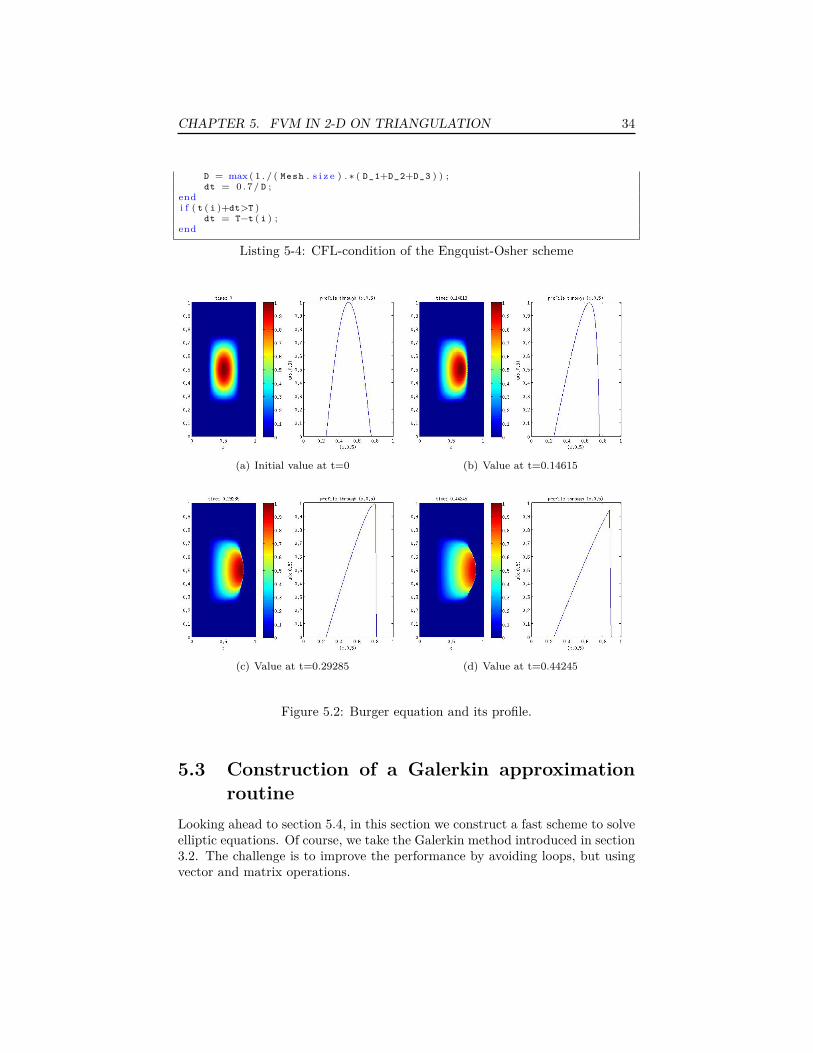
As initial condition, we take a sine curve in the middle of the domain. Figure5.2 shows the resulting movements of this bubble and the profile through the liney = 0.5.To derive the missing CFL-conditions we use equation (4.40), and so we deriveListing 5-4.
D_1 = max ( [ Mesh . edgesize ( : , 1 ) . ∗ sum( Mesh . norm ( : , : , 1 ) . ∗ df ( U ( : , i ) ) , 2 ) ,←z e r o s ( s i z e ( Mesh . edgesize ( : , 1 ) ) ) ] , [ ] , 2 ) ;
D_2 = max ( [ Mesh . edgesize ( : , 2 ) . ∗ sum( Mesh . norm ( : , : , 2 ) . ∗ df ( U ( : , i ) ) , 2 ) ,←z e r o s ( s i z e ( Mesh . edgesize ( : , 2 ) ) ) ] , [ ] , 2 ) ;
D_3 = max ( [ Mesh . edgesize ( : , 3 ) . ∗ sum( Mesh . norm ( : , : , 3 ) . ∗ df ( U ( : , i ) ) , 2 ) ,←z e r o s ( s i z e ( Mesh . edgesize ( : , 3 ) ) ) ] , [ ] , 2 ) ;
D = max ( 1 . / ( Mesh . s i z e ) . ∗ ( D_1+D_2+D_3 ) ) ;i f ( D >0.1)
dt = 0. 7/ D ;e l s e
D_1 = max ( [ Mesh . edgesize ( : , 1 ) . ∗ sum( Mesh . norm ( : , : , 1 ) . ∗ MU , 2 ) , z e r o s (←s i z e ( Mesh . edgesize ( : , 1 ) ) ) ] , [ ] , 2 ) ;
D_2 = max ( [ Mesh . edgesize ( : , 2 ) . ∗ sum( Mesh . norm ( : , : , 2 ) . ∗ MU , 2 ) , z e r o s (←s i z e ( Mesh . edgesize ( : , 2 ) ) ) ] , [ ] , 2 ) ;
D_3 = max ( [ Mesh . edgesize ( : , 3 ) . ∗ sum( Mesh . norm ( : , : , 3 ) . ∗ MU , 2 ) , z e r o s (←s i z e ( Mesh . edgesize ( : , 3 ) ) ) ] , [ ] , 2 ) ;
CHAPTER 5. FVM IN 2-D ON TRIANGULATION 34
D = max ( 1 . / ( Mesh . s i z e ) . ∗ ( D_1+D_2+D_3 ) ) ;dt = 0. 7/ D ;
endi f ( t ( i )+dt>T )
dt = T−t ( i ) ;end
Listing 5-4: CFL-condition of the Engquist-Osher scheme
(a) Initial value at t=0 (b) Value at t=0.14615
(c) Value at t=0.29285 (d) Value at t=0.44245
Figure 5.2: Burger equation and its profile.
5.3 Construction of a Galerkin approximationroutine
Looking ahead to section 5.4, in this section we construct a fast scheme to solveelliptic equations. Of course, we take the Galerkin method introduced in section3.2. The challenge is to improve the performance by avoiding loops, but usingvector and matrix operations.

CHAPTER 5. FVM IN 2-D ON TRIANGULATION 35
We implement two different functions, which calculate the element stiffness ma-trix (3.20) and the load vector (3.18).
5.3.1 Element stiffness matrixTo get the element stiffness matrix, we use equation (3.27). First we calculatethe inverse of BK and its determinant, where invBK1_ (i, j) = B−1
K (1, j) andinvBK2_(i, j) = B−1
K (2, j) for the ith element.Then, to get the resulting matrix A, we compute the local matrix aK and finallyassemble the global one (Listing 5-5). One important fact is, that the functionF is piecewise constant. Therefore it is much easier to integrate it.
f u n c t i o n [ A ] = As sem bly _ma t ( Mesh , F )
% t h i s are v e c t o r s which s a f e the c o o r d i n a t e s f o r the i−th v e r t e x% from every elementVert1 = Mesh . Coordinates ( Mesh . Elements ( : , 1 ) , : ) ;Vert2 = Mesh . Coordinates ( Mesh . Elements ( : , 2 ) , : ) ;Vert3 = Mesh . Coordinates ( Mesh . Elements ( : , 3 ) , : ) ;
% Element mapping BK = [ a , b ; c , d ]a = Vert2 ( : , 1 )−Vert1 ( : , 1 ) ;c = Vert2 ( : , 2 )−Vert1 ( : , 2 ) ;b = Vert3 ( : , 1 )−Vert1 ( : , 1 ) ;d = Vert3 ( : , 2 )−Vert1 ( : , 2 ) ;
invBK1_ = [ a ~=0, a ~ = 0 ] . ∗ [ 1 . / ( a+(a==0))+c . ∗ b . / ( ( d . ∗ ( a . ^ 2 )−c . ∗ b . ∗ a ) +(( d←. ∗ ( a . ^ 2 )−c . ∗ b . ∗ a )==0)) ,−b . / ( ( d . ∗ a−c . ∗ b ) +(( d . ∗ a−c . ∗ b )==0)) ] ;
invBK1_ = invBK1_ +[a==0,a ==0].∗[−d . / ( ( b . ∗ c ) +(( b . ∗ c )==0)) , 1 . / ( c+(c==0))←] ;
invBK2_ = [ a ~=0, a ~=0].∗ [− c . / ( ( a . ∗ d−c . ∗ b ) +(( a . ∗ d−c . ∗ b )==0)) , a . / ( ( d . ∗ a−c←. ∗ b ) +(( d . ∗ a−c . ∗ b )==0)) ] ;
invBK2_ = invBK2_ +[a==0,a = = 0 ] . ∗ [ 1 . / ( b+(b==0)) , z e r o s ( s i z e ( b ) ) ] ;
detBK = abs ( a . ∗ d−b . ∗ c ) ;
% c a l c u l a t i n g the l o c a l matrixi11 = invBK1_ ( : , 1 ) ;i12 = invBK1_ ( : , 2 ) ;i21 = invBK2_ ( : , 1 ) ;i22 = invBK2_ ( : , 2 ) ;
A11 = 1/2∗ detBK . ∗ ( F ( : , 1 ) . ∗ i11 .^2+ F ( : , 2 ) . ∗ i12 .^2+2∗ F ( : , 1 ) . ∗ i11 . ∗ i21+2∗F←( : , 2 ) . ∗ i12 . ∗ i22+F ( : , 1 ) . ∗ i21 .^2+ F ( : , 2 ) . ∗ i22 . ^ 2 ) ;
A12 = 1/2∗ detBK .∗(− F ( : , 1 ) . ∗ i11 .^2−F ( : , 2 ) . ∗ i12 .^2−F ( : , 1 ) . ∗ i11 . ∗ i21−F←( : , 2 ) . ∗ i12 . ∗ i22 ) ;
A13 = 1/2∗ detBK .∗(− F ( : , 1 ) . ∗ i11 . ∗ i21−F ( : , 2 ) . ∗ i12 . ∗ i22−F ( : , 1 ) . ∗ i21 .^2−F←( : , 2 ) . ∗ i22 . ^ 2 ) ;
A21 = 1/2∗ detBK .∗(− F ( : , 1 ) . ∗ i11 .^2−F ( : , 2 ) . ∗ i12 .^2−F ( : , 1 ) . ∗ i11 . ∗ i21−F←( : , 2 ) . ∗ i12 . ∗ i22 ) ;
A22 = 1/2∗ detBK . ∗ ( F ( : , 1 ) . ∗ i11 .^2+ F ( : , 2 ) . ∗ i12 . ^ 2 ) ;A23 = 1/2∗ detBK . ∗ ( F ( : , 1 ) . ∗ i11 . ∗ i21+F ( : , 2 ) . ∗ i12 . ∗ i22 ) ;A31 = 1/2∗ detBK .∗(− F ( : , 1 ) . ∗ i11 . ∗ i21−F ( : , 2 ) . ∗ i12 . ∗ i22−F ( : , 1 ) . ∗ i21 .^2−F←
( : , 2 ) . ∗ i22 . ^ 2 ) ;A32 = 1/2∗ detBK . ∗ ( F ( : , 1 ) . ∗ i11 . ∗ i21+F ( : , 2 ) . ∗ i12 . ∗ i22 ) ;A33 = 1/2∗ detBK . ∗ ( F ( : , 1 ) . ∗ i21 .^2+ F ( : , 2 ) . ∗ i22 . ^ 2 ) ;
% assemble the m a t r i c e sI = z e r o s (9∗ s i z e ( Mesh . Elements , 1 ) , 1 ) ;J = z e r o s (9∗ s i z e ( Mesh . Elements , 1 ) , 1 ) ;A = z e r o s (9∗ s i z e ( Mesh . Elements , 1 ) , 1 ) ;

CHAPTER 5. FVM IN 2-D ON TRIANGULATION 36
I = [ Mesh . Elements ( : , 1 ) ; Mesh . Elements ( : , 1 ) ; Mesh . Elements ( : , 1 ) ; Mesh .←Elements ( : , 2 ) ; Mesh . Elements ( : , 2 ) ; Mesh . Elements ( : , 2 ) ; Mesh . Elements←( : , 3 ) ; Mesh . Elements ( : , 3 ) ; Mesh . Elements ( : , 3 ) ] ;
J = [ Mesh . Elements ( : , 1 ) ; Mesh . Elements ( : , 2 ) ; Mesh . Elements ( : , 3 ) ; Mesh .←Elements ( : , 1 ) ; Mesh . Elements ( : , 2 ) ; Mesh . Elements ( : , 3 ) ; Mesh . Elements←( : , 1 ) ; Mesh . Elements ( : , 2 ) ; Mesh . Elements ( : , 3 ) ] ;
A = [ A11 ; A12 ; A13 ; A21 ; A22 ; A23 ; A31 ; A32 ; A33 ] ;A = s p a r s e ( I , J , A ) ;
Listing 5-5: Computing the element stiffness matrix
5.3.2 Load vectorCalculate the load vector of a piecewise constant function is not a too difficulttask. Again, we first calculate the local Load vector and sum it up afterwards.But now, we do not need the BK matrix, we just need the determinant of it.So we get the function Assembly_Load_PC (Listing 5-6).
f u n c t i o n [ L ] = A s s e m b l y _ L o a d _ P C ( Mesh , F )% B u i l t the load v e c t o r o f the p i e c e w i s e constant f u n c t i o n f , where f% i s a vector , which s t o r e s f o r each element i the value f ( i ) .
% t h i s are v e c t o r s which s a f e the c o o r d i n a t e s f o r the i−th v e r t e x% from every elementVert1 = Mesh . Coordinates ( Mesh . Elements ( : , 1 ) , : ) ;Vert2 = Mesh . Coordinates ( Mesh . Elements ( : , 2 ) , : ) ;Vert3 = Mesh . Coordinates ( Mesh . Elements ( : , 3 ) , : ) ;
% c a l c u l a t i n g the i n t e g r a l o f the l o c a l load v e c t o rdetBK = abs ( ( Vert2 ( : , 1 )−Vert1 ( : , 1 ) ) . ∗ ( Vert3 ( : , 2 )−Vert1 ( : , 2 ) )−(Vert3←
( : , 1 )−Vert1 ( : , 1 ) ) . ∗ ( Vert2 ( : , 2 )−Vert1 ( : , 2 ) ) ) ;Lloc1 = detBK . ∗ F ∗1/6 ;Lloc2 = detBK . ∗ F ∗1/6 ;Lloc3 = detBK . ∗ F ∗1/6 ;
% assemble the load v e c t o r sL = z e r o s ( s i z e ( Mesh . Coordinates , 1 ) , 1 ) ;f o r i = 1 : s i z e ( Mesh . Elements , 1 )
L ( Mesh . Elements ( i , 1 ) ) = L ( Mesh . Elements ( i , 1 ) )+Lloc1 ( i ) ;L ( Mesh . Elements ( i , 2 ) ) = L ( Mesh . Elements ( i , 2 ) )+Lloc2 ( i ) ;L ( Mesh . Elements ( i , 3 ) ) = L ( Mesh . Elements ( i , 3 ) )+Lloc3 ( i ) ;
end
Listing 5-6: Computing the load vector
5.4 Simulation of flow in porous mediaSucceeding in implementing the finite volume routine, we like to test it on reser-voir models. In this section we present some complete simulators for reservoirsimulation. We look at the following problems of different difficulty:
• incompressible single-phase flow,
• incompressible two-phase flow with some assumptions,

CHAPTER 5. FVM IN 2-D ON TRIANGULATION 37
• incompressible two-phase flow with data from 10th SPE Comparative So-lution Project [9].
The following examples are based on the examples from J. E. Aarnes, T. Gimseand K. Lie in [5], who have used different solvers. In this chapter, we work withno-flow boundary condition, this means that we need another triangulation.Hence, we use Listing 5-1 and use Listing 5-7 for the boundary condition.
f u n c t i o n [ Mesh ]= NFBddCond ( Mesh , dt , fe , xe , ye , n0 , a_x , a_y )% C a l c u l a t e boundary c o n d i t i o n f o r no−f low c o n d i t i o n on% [ 0 , a_x ] x [ 0 , a_y ]f o r i = 1 : n0
a = e d g e A t t a c h m e n t s ( dt , fe ( : , i ) ' ) ;a = a : ;x_i = xe ( : , i ) ;y_i = ye ( : , i ) ;check = 0 ;f o r j =1:3
i f ( i snan ( Mesh . Neighbors ( a , j ) )==1&&check==0)Mesh . Neighbors ( a , j )=a ;i f ( y_i ==[0;0 ])
Mesh . norm ( a , : , j ) = [ 0 , −1 ] ;e l s e i f ( y_i==[a_y ; a_y ] )
Mesh . norm ( a , : , j ) = [ 0 , 1 ] ;e l s e i f ( x_i ==[0;0 ])
Mesh . norm ( a , : , j ) = [ −1 , 0 ] ;e l s e i f ( x_i==[a_x ; a_x ] )
Mesh . norm ( a , : , j ) = [ 1 , 0 ] ;endMesh . edgesize ( a , j ) = s q r t ( ( x_i ( 1 )−x_i ( 2 ) ) ^2+( y_i ( 1 )−y_i ( 2 )←
) ^2) ;check = 1 ;
endend
end
Listing 5-7: Construction of no-flow boundary condition
Example 5.2 (Incompressible single-phase flow). As in chapter 2 introduced,for the incompressible single-phase flow, we get the elliptic equation (2.24). Tocreate an example as simple as possible, assume homogeneous and isotropicpermeability K ≡ 1 for all x ∈ R. In this model, we set an injection wellat the origin and production wells at the points (±1,±1) and assume no-flowconditions at the boundary of [−1, 1]× [−1, 1]. In the model of the single-phaseflow, we have an initially filled domain with fluid. We inject additional fluid atthe injection well. Due to this injection the fluid is pushed out at the productionwells. The flow in this five-spot domain is symmetric about both the coordinateaxes. Therefore, we can reduce this model to a model on the domain [0, 1]2 withonly one injection well and one production well at (0, 0) and (1, 1). This iscalled a quarter-five spot problem.The pressure p is calculated by first evaluating the element stiffness matrix Ausing Listening ?? and 5-5, then the load vector L by Listening 5-6 and in theend solving the linear equation:
Ap = L. (5.3)
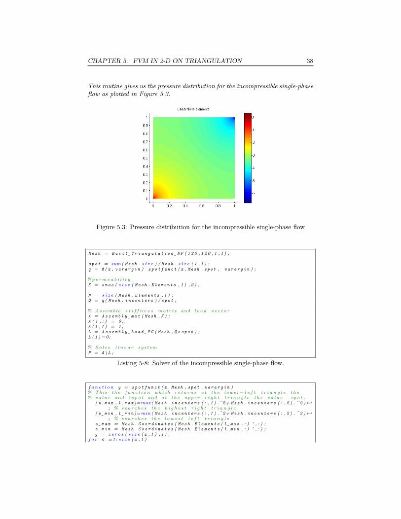
CHAPTER 5. FVM IN 2-D ON TRIANGULATION 38
This routine gives us the pressure distribution for the incompressible single-phaseflow as plotted in Figure 5.3.
Figure 5.3: Pressure distribution for the incompressible single-phase flow
M e s h = B u i l t _ T r i a n g u l a t i o n _ N F ( 1 2 0 , 1 2 0 , 1 , 1 ) ;
s p o t = sum ( M e s h . s i z e ) / M e s h . s i z e ( 1 , 1 ) ;q = @ ( x , v a r a r g i n ) s p o t f u n c t ( x , Mesh , spot , v a r a r g i n ) ;
%p e r m e a b i l i t yK = o n e s ( s i z e ( M e s h . E l e m e n t s , 1 ) , 2 ) ;
N = s i z e ( M e s h . E l e m e n t s , 1 ) ;Q = q ( M e s h . i n c e n t e r s ) / s p o t ;
% Assemble s t i f f n e s s matr ix and l o a d v e c t o rA = A s s e m b l y _ m a t ( Mesh , K ) ;A ( 1 , : ) = 0 ;A ( 1 , 1 ) = 1 ;L = A s s e m b l y _ L o a d _ P C ( Mesh , Q ∗ s p o t ) ;L ( 1 ) =0;
% S o l v e l i n e a r systemP = A \ L ;
Listing 5-8: Solver of the incompressible single-phase flow.
f u n c t i o n y = s p o t f u n c t ( x , Mesh , spot , v a r a r g i n )% This t h e f u n c t i o n which r e t u r n s a t t h e lower− l e f t t r i a n g l e t h e% v a l u e and +s p o t and a t t h e upper−r i g h t t r i a n g l e t h e v a l u e −s p o t .
[ v _ m a x , l _ m a x ]=max( M e s h . i n c e n t e r s ( : , 1 ) .^2+ M e s h . i n c e n t e r s ( : , 2 ) . ^ 2 )←; % s e a r c h e s t h e h i g h e s t r i g h t t r i a n g l e
[ v _ m i n , l _ m i n ]=min ( M e s h . i n c e n t e r s ( : , 1 ) .^2+ M e s h . i n c e n t e r s ( : , 2 ) . ^ 2 )←; % s e a r c h e s t h e l o w e s t l e f t t r i a n g l e
a _ m a x = M e s h . C o o r d i n a t e s ( M e s h . E l e m e n t s ( l _ m a x , : ) ' , : ) ;a _ m i n = M e s h . C o o r d i n a t e s ( M e s h . E l e m e n t s ( l _ m i n , : ) ' , : ) ;y = z e r o s ( s i z e ( x , 1 ) , 1 ) ;
f o r i =1: s i z e ( x , 1 )

CHAPTER 5. FVM IN 2-D ON TRIANGULATION 39
i f ( d i s t _ t r i ( x ( i , : ) , a _ m a x ( 1 , : ) , a _ m a x ( 2 , : ) , a _ m a x ( 3 , : ) )<=0)y ( i , 1 ) = −1∗ s p o t ;
e l s e i f ( d i s t _ t r i ( x ( i , : ) , a _ m i n ( 1 , : ) , a _ m i n ( 2 , : ) , a _ m i n ( 3 , : ) )<=0)y ( i , 1 ) = 1∗ s p o t ;
e l s ey ( i , 1 ) = 0 ;
endend
f u n c t i o n d i s t = d i s t _ t r i ( x , a , b , c )%c a l c u l a t e s t h e d i s t a n c e o f x and t h e t r i a n g l e d e f i n e d% by t h e p t s a , b , c
d i s t = −min ( min ( ( ( x ( : , 1 )−a ( 1 ) ) ∗( a ( 2 )−b ( 2 ) )−(x ( : , 2 )−a ( 2 ) ) ∗( a ( 1 )−←b ( 1 ) ) ) /norm ( a−b ) , . . .
( ( x ( : , 1 )−b ( 1 ) ) ∗( b ( 2 )−c ( 2 ) )−(x ( : , 2 )−b ( 2 ) ) ∗( b ( 1 )−c ( 1 ) ) ) /norm←( b−c ) ) , . . .
( ( x ( : , 1 )−c ( 1 ) ) ∗( c ( 2 )−a ( 2 ) )−(x ( : , 2 )−c ( 2 ) ) ∗( c ( 1 )−a ( 1 ) ) ) /norm←( c−a ) ) ;
r e t u r n
Listing 5-9: Injection and production term.
Since the incompressible single-phase flow is a trivial case, we take now a lookat a more complex example, the immiscible and incompressible two-phase flow.Example 5.3 (Immiscible and incompressible two-phase flow). The immiscibleand incompressible two-phase flow was introduced in section 2.3. In addition letus consider the setting of example 2.1, the quarter-five spot as before, no-flowboundary condition and that it takes one time unit to inject one pore-volume ofwater. In this model, the reservoir is initially filled with oil and we simulatea water injection at (0, 0). When solving the problem, we solve the almost-elliptic pressure equation (2.43) and the almost-hyperbolic saturation equation(2.47). This equations are nonlinearly coupled primarily through the saturationdependent mobility λi and the pressure dependent velocity vi. For simplicity, wedisregard the gravity and capillary forces. So we get the following equations:
−∇ ·Kλ(s)∇p = Qt, (5.4)
φ∂s
∂t+∇ · (f(s)v) = qw
ρw. (5.5)
The strategy is to solve the two equations sequentially by the two routines derivedin the previous sections 5.2 and 5.3. As long as we only inject water, and producewhatever reaches our production well, we get:
qwρw
= maxQt, 0+ f(s)minQt, 0. (5.6)
For the last missing saturation dependent quantities, we use:
λw(s) = (s∗)2
µw, λo(s) = (1−s∗)2
µo, s∗ = s−swc
1−sor−swc,
where sor is the lowest oil saturation, that can be achieved by displacing oil bywater, and swc is the connate water saturation. To keep the problem still simple,we assume furthermore unit porosity, unit viscosity and set sor = swc = 0.The solver of Example 5.2 can be used for the elliptic part by updating it. Insteadof K we now use Kλ. The procedure of our solver is:

CHAPTER 5. FVM IN 2-D ON TRIANGULATION 40
• solve the elliptic pde;
• calculate the velocity v = Kλ(s)∇p, where ∇p is the discrete gradient,Listing 5-10;
• solve the hyperbolic problem between 0 and ∆t, Listing 5-11;
• solve the elliptic pde with the new saturation;
• calculate the velocity v, Listing 5-10;
• solve the hyperbolic problem between ∆t and 2∆t, Listing 5-11;
• . . .
• solve the elliptic pde with the saturation at final time T .
Listing 5-12 contains the code to simulate all of this. For calculating the timesteps, we use the CFL-condition calculated by equation (4.40). We choose somedefinitions a little bit more general, such that we can upgrade the code easily.
f u n c t i o n V = V e l o T r i ( P , Mesh , Kf , l a m b d a , s )% C a l c u l a t e v v e l o c i t y on Mesh g r i da _ 1 = ( P ( M e s h . E l e m e n t s ( : , 1 ) )−P ( M e s h . E l e m e n t s ( : , 2 ) ) ) . ∗ ( M e s h .←
C o o r d i n a t e s ( M e s h . E l e m e n t s ( : , 3 ) , 2 )−M e s h . C o o r d i n a t e s ( M e s h .←E l e m e n t s ( : , 2 ) , 2 ) )−(P ( M e s h . E l e m e n t s ( : , 3 ) )−P ( M e s h . E l e m e n t s ( : , 2 ) )←) . ∗ ( M e s h . C o o r d i n a t e s ( M e s h . E l e m e n t s ( : , 1 ) , 2 )−M e s h . C o o r d i n a t e s (←M e s h . E l e m e n t s ( : , 2 ) , 2 ) ) ;
a _ 2 = ( M e s h . C o o r d i n a t e s ( M e s h . E l e m e n t s ( : , 1 ) , 1 )−M e s h . C o o r d i n a t e s (←M e s h . E l e m e n t s ( : , 2 ) , 1 ) ) . ∗ ( M e s h . C o o r d i n a t e s ( M e s h . E l e m e n t s ( : , 3 )←, 2 )−M e s h . C o o r d i n a t e s ( M e s h . E l e m e n t s ( : , 2 ) , 2 ) )−( M e s h . C o o r d i n a t e s (←M e s h . E l e m e n t s ( : , 3 ) , 1 )−M e s h . C o o r d i n a t e s ( M e s h . E l e m e n t s ( : , 2 ) , 1 ) )←. ∗ ( M e s h . C o o r d i n a t e s ( M e s h . E l e m e n t s ( : , 1 ) , 2 )−M e s h . C o o r d i n a t e s (←M e s h . E l e m e n t s ( : , 2 ) , 2 ) ) ;
b _ 1 = ( P ( M e s h . E l e m e n t s ( : , 1 ) )−P ( M e s h . E l e m e n t s ( : , 2 ) ) ) . ∗ ( M e s h .←C o o r d i n a t e s ( M e s h . E l e m e n t s ( : , 3 ) , 1 )−M e s h . C o o r d i n a t e s ( M e s h .←E l e m e n t s ( : , 2 ) , 1 ) )−(P ( M e s h . E l e m e n t s ( : , 3 ) )−P ( M e s h . E l e m e n t s ( : , 2 ) )←) . ∗ ( M e s h . C o o r d i n a t e s ( M e s h . E l e m e n t s ( : , 1 ) , 1 )−M e s h . C o o r d i n a t e s (←M e s h . E l e m e n t s ( : , 2 ) , 1 ) ) ;
b _ 2 = −a _ 2 ;
V = −Kf . ∗ [ l a m b d a ( s ) , l a m b d a ( s ) ] . ∗ [ a _ 1 . / a_2 , b _ 1 . / b _ 2 ] ;end
Listing 5-10: Computation of velocity using the pressure, v = Kλ(s)∇p.
f u n c t i o n [ s , t ]= E O S ( s0 , t0 , d e l t a _ t , V , f , df , Q , phi , Mesh , s_wc , s _ o r )% s o l v e s t h e h y p e r b o l i c e q u a t i o n by u s i n g t h e e n g q u i s t o s h e r ←
scheme between% t 0 and t 0+d e l t a _ t w i t h i n i t i a l v a l u e s0N = s i z e ( M e s h . E l e m e n t s , 1 ) ;t =0;st=s0 ;w h i l e ( t<d e l t a _ t )
q w _ o v e r _ r h o w = max ( [ Q , z e r o s ( s i z e ( Q ) ) ] , [ ] , 2 )+f ( st ) . ∗ min ( [ Q ,←z e r o s ( s i z e ( Q ) ) ] , [ ] , 2 ) ;
% CFL−c o n d i t i o nD _ 1 = max ( [ M e s h . e d g e s i z e ( : , 1 ) . ∗ sum ( M e s h . norm ( : , : , 1 ) . ∗ df ( st , V←
( : , 1 ) , V ( : , 2 ) ) , 2 ) , z e r o s ( s i z e ( M e s h . e d g e s i z e ( : , 1 ) ) ) ] , [ ] , 2 ) ;

CHAPTER 5. FVM IN 2-D ON TRIANGULATION 41
D _ 2 = max ( [ M e s h . e d g e s i z e ( : , 2 ) . ∗ sum ( M e s h . norm ( : , : , 2 ) . ∗ df ( st , V←( : , 1 ) , V ( : , 2 ) ) , 2 ) , z e r o s ( s i z e ( M e s h . e d g e s i z e ( : , 2 ) ) ) ] , [ ] , 2 ) ;
D _ 3 = max ( [ M e s h . e d g e s i z e ( : , 3 ) . ∗ sum ( M e s h . norm ( : , : , 3 ) . ∗ df ( st , V←( : , 1 ) , V ( : , 2 ) ) , 2 ) , z e r o s ( s i z e ( M e s h . e d g e s i z e ( : , 3 ) ) ) ] , [ ] , 2 ) ;
D = max ( 1 . / ( M e s h . s i z e . ∗ p h i ) . ∗ ( D _ 1+D _ 2+D _ 3 +1) ) ;i f ( D >0.1)
dt = 0 . 7 / D ;e l s e
D _ 1 = max ( [ M e s h . e d g e s i z e ( : , 1 ) . ∗ sum ( M e s h . norm ( : , : , 1 ) . ∗ df ( 2 ,←V ( : , 1 ) , V ( : , 2 ) ) , 2 ) , z e r o s ( s i z e ( M e s h . e d g e s i z e ( : , 1 ) ) )←] , [ ] , 2 ) ;
D _ 2 = max ( [ M e s h . e d g e s i z e ( : , 2 ) . ∗ sum ( M e s h . norm ( : , : , 2 ) . ∗ df ( 2 ,←V ( : , 1 ) , V ( : , 2 ) ) , 2 ) , z e r o s ( s i z e ( M e s h . e d g e s i z e ( : , 2 ) ) )←] , [ ] , 2 ) ;
D _ 3 = max ( [ M e s h . e d g e s i z e ( : , 3 ) . ∗ sum ( M e s h . norm ( : , : , 3 ) . ∗ df ( 2 ,←V ( : , 1 ) , V ( : , 2 ) ) , 2 ) , z e r o s ( s i z e ( M e s h . e d g e s i z e ( : , 3 ) ) )←] , [ ] , 2 ) ;
D = max ( 1 . / ( M e s h . s i z e . ∗ p h i ) . ∗ ( D _ 1+D _ 2+D _ 3 +1) ) ;dt = 0 . 7 / D ;
endi f ( t+dt>d e l t a _ t )
dt=d e l t a _ t−t ;endt = t+dt ;% c a l c u l a t i o n o f t h e FluxG _ 1 = abs ( M e s h . e d g e s i z e ( : , 1 ) ) . ∗ ( f ( st ) . ∗ max( sum ( M e s h . norm←
( : , : , 1 ) . ∗ V , 2 ) , z e r o s ( N , 1 ) )+f ( st ( M e s h . N e i g h b o r s ( : , 1 ) ) ) . ∗ min (←sum ( M e s h . norm ( : , : , 1 ) . ∗ V , 2 ) , z e r o s ( N , 1 ) ) ) ;
G _ 2 = abs ( M e s h . e d g e s i z e ( : , 2 ) ) . ∗ ( f ( st ) . ∗ max( sum ( M e s h . norm←( : , : , 2 ) . ∗ V , 2 ) , z e r o s ( N , 1 ) )+f ( st ( M e s h . N e i g h b o r s ( : , 2 ) ) ) . ∗ min (←sum ( M e s h . norm ( : , : , 2 ) . ∗ V , 2 ) , z e r o s ( N , 1 ) ) ) ;
G _ 3 = abs ( M e s h . e d g e s i z e ( : , 3 ) ) . ∗ ( f ( st ) . ∗ max( sum ( M e s h . norm←( : , : , 3 ) . ∗ V , 2 ) , z e r o s ( N , 1 ) )+f ( st ( M e s h . N e i g h b o r s ( : , 3 ) ) ) . ∗ min (←sum ( M e s h . norm ( : , : , 3 ) . ∗ V , 2 ) , z e r o s ( N , 1 ) ) ) ;
st = st − dt . / ( M e s h . s i z e . ∗ p h i ) . ∗ ( G _ 1+G _ 2+G _ 3 )+dt . ∗ q w _ o v e r _ r h o w←. / ( M e s h . s i z e . ∗ p h i ) ;
st = max(−(1− s _ w c ) , min(1− s_wc , st ) ) ;ends=st ;t=t0+d e l t a _ t ;end
Listing 5-11: Solver of the hyperbolic problem between t0 and t0+delta_t usingthe Engquist-Osher scheme.
%Main code
M e s h = B u i l t _ T r i a n g u l a t i o n _ N F ( 1 2 0 , 1 2 0 , 1 , 1 ) ;
T = 1 ; %End timek = 1/25; % time s t e p a f t e r which t h e e l l i p t i c e q u a t i o n i s s o l v e dnt = T / k ; % number o f t i m e s t h e e l l i p t i c e q u a t i o n i s s o l v e d .s _ w c = 0 ;s _ o r = 0 ;m u _ w = 1 ;m u _ o = 1 ;n =1;l a m b d a _ o = @ ( s ) (1−(s−s _ w c ) ./(1− s_or−s _ w c ) ) . ^ 2 / m u _ o ;l a m b d a _ w = @ ( s ) ( ( s−s _ w c ) ./(1− s_or−s _ w c ) ) . ^ 2 / m u _ w ;l a m b d a = @ ( s ) l a m b d a _ o ( s )+l a m b d a _ w ( s ) ;f = @ ( s ) l a m b d a _ w ( s ) . / l a m b d a ( s ) ;df = @ ( s , u , v ) [ 2 ∗ m u _ w ∗ m u _ o ∗( s+s_or −1) . ∗ ( s−s _ w c ) ∗( s _ o r+s_wc −1) . / (←
m u _ w ∗( s+s_or −1) .^2+ m u _ o ∗( s−s _ w c ) . ^ 2 ) . ^ 2 . ∗ u , 2 ∗ m u _ w ∗ m u _ o ∗( s+s_or←−1) . ∗ ( s−s _ w c ) ∗( s _ o r+s_wc −1) . / ( m u _ w ∗( s+s_or −1) .^2+ m u _ o ∗( s−s _ w c )←. ^ 2 ) . ^ 2 . ∗ v ] ;

CHAPTER 5. FVM IN 2-D ON TRIANGULATION 42
I = [ 0 , −1 ; 1 , 0 ] ;s = s _ w c ∗ o n e s ( s i z e ( M e s h . E l e m e n t s , 1 ) , 1 ) ; %i n i t i a l s a t u r a t i o n
s p o t = sum ( M e s h . s i z e ) / M e s h . s i z e ( 1 , 1 ) ;q = @ ( x , v a r a r g i n ) s p o t f u n c t ( x , Mesh , spot , v a r a r g i n ) ;% P e r m e a b i l i t yKf = o n e s ( s i z e ( M e s h . E l e m e n t s , 1 ) , 2 ) ;p h i = o n e s ( s i z e ( M e s h . E l e m e n t s , 1 ) , 1 ) ;N = s i z e ( M e s h . E l e m e n t s , 1 ) ;Q = q ( M e s h . i n c e n t e r s ) / s p o t ;
%% Assemble s t i f f n e s s matr ix and l o a d v e c t o r a t t ime t 0 = 0K = [ l a m b d a ( s ( : , 1 ) ) , l a m b d a ( s ( : , 1 ) ) ] . ∗ Kf ;A = A s s e m b l y _ m a t ( Mesh , K ) ;A ( 1 , : ) = 0 ;A ( 1 , 1 ) = 1 ;L = A s s e m b l y _ L o a d _ P C ( Mesh , Q ∗ s p o t ) ;L ( 1 ) =0;
% S o l v e l i n e a r systemP = z e r o s ( s i z e ( M e s h . C o o r d i n a t e s , 1 ) , nt +1) ;P ( : , 1 ) = A \ L ;
% C a l c u l a t e v v e l o c i t y on GridV=V e l o T r i ( P ( : , 1 ) , Mesh , Kf , l a m b d a , s ( : , 1 ) ) ;
%% Time s t e p p i n gt =0;f o r i = 1 : nt
i% S o l v e h y p e r b o l i c p a r t between t and t+k[ s ( : , i +1) , t ] = E O S ( s ( : , i ) , t , k , V , f , df , Q ∗ spot , phi , Mesh , s_wc , s _ o r←
) ;
% Assemble s t i f f n e s s matr ix and l o a d v e c t o r a t t ime i ∗ kK = [ l a m b d a ( s ( : , i +1) ) , l a m b d a ( s ( : , i +1) ) ] . ∗ Kf ;A = A s s e m b l y _ m a t ( Mesh , K ) ;A ( 1 , : ) = 0 ;A ( 1 , 1 ) = 1 ;L = A s s e m b l y _ L o a d _ P C ( Mesh , Q ∗ s p o t ) ;L ( 1 ) = 1 ;
% S o l v e l i n e a r systemP ( : , i +1) = A \ L ;
% C a l c u l a t e v v e l o c i t y on Mesh g r i dV=V e l o T r i ( P ( : , i +1) , Mesh , Kf , l a m b d a , s ( : , i +1) ) ;
end
Listing 5-12: Simulator for the immiscible and incompressible two-phase flow.
The saturation distribution computed by Listing 5-12 is shown in figure 5.4. Theappropriate functionality of the implementation is established by the followingtwo results. The first is, that the basic structure looks correct. And the secondis, that the theoretical value of the break through, the time at which the waterfirst reaches the production well, coincides with the theoretical value, what isapproximately 0.7 pore-volumes of water [5].If you look at the exact shape of the water wave, you will recognize first a shockwave and after this a monotonically increasing saturation.Comparing the L1-error over time and space of the solution computed by theprogram of this thesis and the solution of J. E. Aarnes, T. Gimse and K. A.Lie in [5] we get a sublinear convergence plotted in figure 5.5.

CHAPTER 5. FVM IN 2-D ON TRIANGULATION 43
(a) Value at t=0.08 (b) Value at t=0.24 (c) Value at t=0.40
(d) Value at t=0.56 (e) Value at t=0.72 (f) Value at t=0.84
Figure 5.4: Saturation profiles for the homogeneous quarter-five spot.
Example 5.4 (Simulation of the SPE-model by using finite volume method).In the example 5.3, we still looked at a simplified two-phase model. Let us takea look at a much more realistic setting of porosity and permeability, by look-ing at the model 2 from the 10th SPE Comparative Solution Project [9]. Themodel dimensions are 1200 × 2200 × 170 (ft) and the reservoir is described bya heterogeneous distribution over a regular Cartesian grid with 60 × 220 × 85grid-blocks. Because we use a triangular mesh, we have to transform this to atriangular grid, Listing 5-13. We use only the top layer, in which the perme-ability is smooth. We set again the injection well at the lower-left corner andthe production well at the upper-right one. For brevity, gravity and capillaryforces are neglect. And we consider a incompressible oil-water system, for whichswc = sor = 0.2, µw = 0.3 cp and µo = 3.0 cp. The reservoir is initially filledwith oil, this means that the initial water saturation is equal the connate watersaturation. Since the porosity is not uniform anymore, it may be zero. To avoiddivision by zero, we set it to a minimal nonzero value.
Figure 5.6 shows the saturation distribution over the first 2000 days computedby Listing 5-14. Figure 5.7 shows the distribution computed by J. E. Aarnes,T. Gimse and K. A. Lie in [5]. By comparing the different results, it is obviousthat in our solution the water is much faster than in the solution of [5]. Thedifference between the simulated flows occurs probably from a different settingof parameters. By comparing the different production rates (figure 5.8), you seethat the presented algorithm in this thesis yields the correct behavior.Comparing the derived code of this thesis and the code given in [9], you notice

CHAPTER 5. FVM IN 2-D ON TRIANGULATION 44
Figure 5.5: Rate of convergence for the immiscible and incompressible two-phaseflow
that the original code is much faster than this one. The reason is, that they usean implicit solver, in comparison to our explicit solver. In a implicit solver thediscretization is a large nonlinear system of equations, which are usually solvedwith a Newton or a Newton-Raphson iterative method. The problem with explicitsolvers is that for convergence, we need to fulfill a CFL-condition, which in theheterogeneous case gives us really tiny time steps. So in this case an implicitsolver would be faster.
f u n c t i o n [ phi , Kf ] = l o a d _ P h i _ P e r m ( Mesh , s p e _ p e r m , s p e _ p h i )% Transformation o f t h e p e r m e a b i l i t y perm and p o r o s i t y p h i t o t h e% t r i a n g u l a r meshl o a d s p e _ p e r m . d a t ; l o a d s p e _ p h i . d a t ;p e r m 2 = r e s h a p e ( s p e _ p e r m ' , s i z e ( s p e _ p e r m , 1 ) ∗2 ,3) ;p e r m = z e r o s ( 6 0 , 2 2 0 , 2 ) ;f o r i = 1 : 6 0 , f o r j = 0 : 2 1 9 , l = 0 ; p e r m ( i , j +1 ,1) = p e r m 2 ( i+j∗60+l←
∗220∗60 ,1) ; end , endf o r i = 1 : 6 0 , f o r j = 0 : 2 1 9 , l = 0 ; p e r m ( i , j +1 ,2) = p e r m 2 ( i+j∗60+l←
∗220∗60 ,2) ; end , end
s p e _ p h i 2 = r e s h a p e ( s p e _ p h i ' , s i z e ( s p e _ p h i , 1 ) ∗ s i z e ( s p e _ p h i , 2 ) , 1 ) ;p h i = z e r o s ( 6 0 , 2 2 0 , 8 5 ) ;f o r i = 1 : 6 0 , f o r j = 0 : 2 1 9 , f o r l = 0 , p h i ( i , j +1 ,1 ) = s p e _ p h i 2 ( i←
+j∗60+l ∗220∗60) ; end , end , endKg=p e r m ; % P e r m e a b i l i t y in l a y e r 1P o r=p h i ( : , : , 1 ) ; % P r e p r o c e s s e d p o r o s i t y in l a y e r 1
Kf = z e r o s ( s i z e ( M e s h . E l e m e n t s , 1 ) , 2 ) ;p h i = z e r o s ( s i z e ( M e s h . E l e m e n t s , 1 ) , 1 ) ;f o r i = 1 : s i z e ( M e s h . E l e m e n t s , 1 )
p h i ( i ) = P o r ( f l o o r ( M e s h . i n c e n t e r s ( i , 1 ) /20) +1, f l o o r ( M e s h .←i n c e n t e r s ( i , 2 ) /10) +1) ;

CHAPTER 5. FVM IN 2-D ON TRIANGULATION 45
Kf ( i , : ) = Kg ( f l o o r ( M e s h . i n c e n t e r s ( i , 1 ) /20) +1, f l o o r ( M e s h .←i n c e n t e r s ( i , 2 ) /10) +1 ,:) ;
endp h i=max( phi , 1 e−3) ;
Listing 5-13: Transformation of the data of the SPE-10 model to the triangulargrid.
(a) Value after 400 days (b) Value after 800 days
(c) Value after 1200 days (d) Value after 2000 days
Figure 5.6: Saturation profiles in the top layer of the SPE-10 model, computedby Listing 5-14.

CHAPTER 5. FVM IN 2-D ON TRIANGULATION 46
(a) Value after 400 days (b) Value after 800 days
(c) Value after 1200 days (d) Value after 2000 days
Figure 5.7: Saturation profiles in the top layer of the SPE-10 model, computedby J. E. Aarnes, T. Gimse and K. A. Lie in [5].
(a) Solution from Listing 5-14 (b) Solution from [5]
Figure 5.8: Production profiles.

CHAPTER 5. FVM IN 2-D ON TRIANGULATION 47
%Main code
% Construct meshMesh = B u i l t _ T r i a n g u l a t i o n _ N F (120 ,120 ,1200 ,2200) ;spot =795/85∗(120∗120∗2) /(60∗220) ;q = @ ( x , varargin ) spotfunct3 ( x , Mesh , spot , varargin ) ;T = 1000;k = 5 0 ;nt = T/k ;s_wc = 0 . 2 ;s_or = 0 . 2 ;mu_w = 0 . 3 ;%3e−4;mu_o = 3 ;%3e−3;lambda_o = @ ( s ) (1−(s−s_wc ) ./(1− s_or−s_wc ) ) . ^ 2 / mu_o ;lambda_w = @ ( s ) ( ( s−s_wc ) ./(1− s_or−s_wc ) ) . ^ 2 / mu_w ;lambda = @ ( s ) lambda_o ( s )+lambda_w ( s ) ;f = @ ( s ) lambda_w ( s ) . / lambda ( s ) ;df = @ ( s , u , v ) [ 2 ∗ mu_w ∗ mu_o ∗( s+s_or−1) . ∗ ( s−s_wc ) ∗( s_or+s_wc−1) . / ( mu_w ∗(←
s+s_or−1).^2+ mu_o ∗( s−s_wc ) . ^ 2 ) . ^ 2 . ∗ u , 2 ∗ mu_w ∗ mu_o ∗( s+s_or−1) . ∗ ( s−←s_wc ) ∗( s_or+s_wc−1) . / ( mu_w ∗( s+s_or−1).^2+ mu_o ∗( s−s_wc ) . ^ 2 ) . ^ 2 . ∗ v ] ;
I = [ 0 , −1 ; 1 , 0 ] ;s = s_wc ∗ ones ( s i z e ( Mesh . Elements , 1 ) , 1 ) ;%n=1;% Permeabi l i ty and p o r o s i t y[ phi , Kf ] = l o a d _ P h i _ P e r m ( Mesh , spe_perm , spe_phi ) ;
N = s i z e ( Mesh . Elements , 1 ) ;Q = q ( Mesh . incenters ) / spot ;%% Assemble s t i f f n e s s matrix and load v e c t o r at time t0 = 0K = [ lambda ( s ( : , 1 ) ) , lambda ( s ( : , 1 ) ) ] . ∗ Kf ;A = As sem bly _m at ( Mesh , K ) ;A ( 1 , : ) = 0 ;A ( 1 , 1 ) = 1 ;L = A s s e m b l y _ L o a d _ P C ( Mesh , Q∗ spot ) ;L ( 1 ) =0;
% Solve l i n e a r systemP = z e r o s ( s i z e ( Mesh . Coordinates , 1 ) , nt +1) ;P ( : , 1 ) = A\L ;
% C a l c u l a t e v v e l o c i t y on Mesh g r i dV=VeloTri ( P ( : , 1 ) , Mesh , Kf , lambda , s ( : , 1 ) ) ;
%% Time s t e p p i n gt =0;f o r i = 1 : nt
i% Solve h y p e r b o l i c part between t and t+k[ s ( : , i+1) , t ] = EOS ( s ( : , i ) , t , k , V , f , df , Q∗ spot , phi , Mesh , s_wc , s_or ) ;
% Assemble s t i f f n e s s matrix and load v e c t o r at time i ∗kK = [ lambda ( s ( : , i+1) ) , lambda ( s ( : , i+1) ) ] . ∗ Kf ;A = As sem bly _m at ( Mesh , K ) ;A ( 1 , : ) = 0 ;A ( 1 , 1 ) = 1 ;L = A s s e m b l y _ L o a d _ P C ( Mesh , Q∗ spot ) ;L ( 1 ) = 1 ;
% Solve l i n e a r systemP ( : , i+1) = A\L ;
% C a l c u l a t e v v e l o c i t y on Mesh g r i dV=VeloTri ( P ( : , i+1) , Mesh , Kf , lambda , s ( : , i+1) ) ;
end
Listing 5-14: Simulator for the immiscible and incompressible two-phase flowfor the top layer of the SPE-10 model.

CHAPTER 6. CONCLUSION AND FURTHER WORK 48
Chapter 6
Conclusion and furtherwork
The aim of this thesis was to design a routine to solve conservation laws byfinite volume methods on triangular grids. This goal was achieved in chapter 5.The tests of the implementation were successful. The behavior of the Burgersequation, incompressible single-phase flow and incompressible two-phase floware correct and the break-through of the water in example 5.3 fits to theory.The disadvantage of this implementation is the run-time. It is really large, com-pared to the run-time of an implicit method. Possibly there is some potentialof improvement. The other time-consuming part is the building of the triangu-lation.Unfortunately, we could not implement a finite volume method for systems ofconservation laws. But this should work in the same way by using the con-structed triangular mesh of section 5.1.A remaining interesting question is the convergence behavior of the method on atriangular grid compared to a method on a Cartesian grid. As well, it would beinteresting to extend the code by some automatically local refinement or evenlocal grid alignment.Hopefully this thesis will motivate and make curious to develop methods ontriangular grids for more dimensional and complex applications.
Bibliography
[1] D. Braess. Finite Elements. Cambridge University Press, 2007.
[2] G. Chavent and J. Jaffre. Mathematical models and finite elements forreservoir simulation. North Holland, 1982.
[3] M. G. Crandall and A. Majda. The method of fractional steps for conser-vation laws. Numerische Mathematik, 34:285–314, 1980.
[4] L. C. Evans. Partial differential equations. AMS, 2010.
[5] T. Gimse J. E. Aarnes and K. A. Lie. An introduction to the numerics offlow in porous media using matlab. 2007.
[6] D. Kröner. Numerical Schemes for Conservation Laws. Wiley Teubner,1997.
[7] S. N. Kruzkov. First order quasilinear equations in several independentvariables. Math. USSR Sbornik, 10:217–243, 1970.
[8] R. J. LeVeque. Numerical Methods for Conservation Laws. Birkhäuser,1992.
[9] M. Blunt M. Christie. Spe comparative solution project, 2001.http://www.spe.org/web/csp/ (11.06.2012).
[10] D. W. Peaceman. Fundamentals of numerical reservoir simulation. Elsevierscientific publishing company, 1977.
[11] G. Huan Z. Chen and Y. Ma. Computational methods for multiphase flowsin porous media. Society for Industrial and Applied Mathematics (SIAM),2006.