finding faces for gender classi cation using back propagation...
TRANSCRIPT

Finding Faces for Gender Classification using
Back Propagation Neural Networks and
Principal Component Analysis based Recognition
Deepak Madan
Harsh Srivastava
Department of Computer Science and Engineering
National Institute of Technology Rourkela
Rourkela-769 008, Orissa, India

Finding Faces for Gender Classification using
Back Propagation Neural Networks and
Principal Component Analysis based Recognition
A thesis submitted on
9thMay, 2011
in partial fulfillment of the requirements for the degree of
Bachelor of Technology
in
Computer Science and Engineering
by
Deepak Madan
(Roll no. 107CS020)
Harsh Srivastava
(Roll no. 107CS027)
Under the guidance of
Prof. Dr. Banshidhar Majhi
Department of Computer Science and Engineering
National Institute of Technology Rourkela
Rourkela-769 008, Orissa, India
2

National Institute of Technology
Rourkela
Certificate
This is to certify that the project entitled, ‘Finding Faces for Gender Classification
using Back Propagation Neural Networks and Principal Component Anal-
ysis based Recognition’ submitted by Deepak Madan and Harsh Srivastava is
an authentic work carried out by them under my supervision and guidance for the par-
tial fulfillment of the requirements for the award of Bachelor of Technology Degree
in Computer Science and Engineering at National Institute of Technology,
Rourkela.
To the best of my knowledge, the matter embodied in the project has not been sub-
mitted to any other University / Institute for the award of any Degree or Diploma.
Date - 09/05/2011
Rourkela
(Prof. Dr. B. Majhi)
Department of Computer Science and Engineering
3

Acknowledgments
We express our profound gratitude and indebtedness to Prof. Dr. B. Majhi , Depart-
ment of Computer Science and Engineering, NIT Rourkela for introducing the present
topic and for his inspiring intellectual guidance, constructive criticism and valuable sug-
gestion throughout the project work.
We are also thankful to Ms. Sunita Kumary and Ms. Hunny Mehrotra, Depart-
ment of Computer Science and Engineering for guiding and motivating us throughout
the project.
Finally, we would like to thank our parents and colleagues for their support and mo-
tivation to complete this project.
Date - 09/05/2011
Rourkela
Deepak Madan
Harsh Srivastava
4

Abstract
Face Classification system is a computer program which will classify a face into
different categories as per certain criterias. We will be training our systems to
classify the images into two septum. The first would classify the images based on
human or non–human characteristics. The second category of classification would
be classifying the human faces as male or female face. We will implement this using
Back Propagation Neural Network algorithm. This pre-classification will help in
reducing the total time required to recognize an image and hence increasing the
overall speed.
Face Recognition system is a computer applicaton that identifies a face of a person
in a digital image by comparing the face in the image with the facial database of
some trained images. This system can recognize images of a person with emotions
and expressions different with those in the facial database. We will implement this
using a mathematical tool called Principal Component Analysis and Mahalanobis
Distance Algorithm. It can be used for security purposes at restricted places by
granting access to only authorised persons. It can also be used for criminal identi-
fication.
We will develop a system which will focus on recognition of faces of individuals
using the above mentioned algorithms to get better accuracy and speed. We will
first use Back Propagation Neural Networks to classify whether the test image is a
human face or not, and if it is a human face whether it is a male face or a female
face and then we will recognize the image using Principal component analysis. This
will help us in reducing the overhead calculations for non-human images and also in
reducing the database size by maintaining different databases for male and female
faces, as the speed of the system depends widely on the database size.
5

Contents
1 Introduction 8
1.1 Problem Statement . . . . . . . . . . . . . . . . . . . . . . . . . . . . . . 8
1.2 Motivation and Challenges . . . . . . . . . . . . . . . . . . . . . . . . . . 8
2 Face Classification using Neural Networks 10
2.1 Back-Propagation Neural Network Algorithm . . . . . . . . . . . . . . . 13
3 Face Recognition using Principal Component
Analysis 16
3.1 PCA Algorithm . . . . . . . . . . . . . . . . . . . . . . . . . . . . . . . . 17
3.1.1 Eigenface Generation . . . . . . . . . . . . . . . . . . . . . . . . . 17
3.1.2 Covariance Matrix and EigenVectors . . . . . . . . . . . . . . . . 18
3.1.3 Weighted Vector . . . . . . . . . . . . . . . . . . . . . . . . . . . 19
3.2 Reconstruction of Original Images . . . . . . . . . . . . . . . . . . . . . . 20
3.3 Mahalanobis Distance Algorithm . . . . . . . . . . . . . . . . . . . . . . 20
4 Facial Databases 22
5 Analysis and Results 26
5.1 Analysis of Face Classification using Neural Networks . . . . . . . . . . . 26
5.1.1 Human-Non human face Classification . . . . . . . . . . . . . . . 26
5.1.2 Gender Classification . . . . . . . . . . . . . . . . . . . . . . . . . 29
5.2 Analysis of Face Recognition using Principal Component Analysis . . . . 30
5.2.1 Analysis on Yale database: . . . . . . . . . . . . . . . . . . . . . . 30
5.2.2 Analysis on Feret Database: . . . . . . . . . . . . . . . . . . . . . 35
6 Conclusion 37
6
List of Figures
1 Face Classification System Using Neural Networks . . . . . . . . . . . . . 11
2 Basic Block of Back Propagation Neural Network . . . . . . . . . . . . . 13
3 Yale Pics Database . . . . . . . . . . . . . . . . . . . . . . . . . . . . . . 18
4 Eigenaces for Yale Pics . . . . . . . . . . . . . . . . . . . . . . . . . . . . 19
5 Linear Combination of Eigenvectors . . . . . . . . . . . . . . . . . . . . . 20
6 Reconstruction of original faces . . . . . . . . . . . . . . . . . . . . . . . 21
7 Known Faces Databse . . . . . . . . . . . . . . . . . . . . . . . . . . . . 22
8 Yale Database . . . . . . . . . . . . . . . . . . . . . . . . . . . . . . . . . 23
9 FERET Database . . . . . . . . . . . . . . . . . . . . . . . . . . . . . . . 24
10 Animal Faces Database . . . . . . . . . . . . . . . . . . . . . . . . . . . . 25
11 Tuning curve: BPNN . . . . . . . . . . . . . . . . . . . . . . . . . . . . . 26
12 Accuracy Rate : BPNN . . . . . . . . . . . . . . . . . . . . . . . . . . . 27
13 Training Curve BPNN: Yale Database . . . . . . . . . . . . . . . . . . . 28
14 Gender Classification Results . . . . . . . . . . . . . . . . . . . . . . . . 29
15 Manual Cropping . . . . . . . . . . . . . . . . . . . . . . . . . . . . . . . 30
16 Conventional Triangularization Approach . . . . . . . . . . . . . . . . . . 30
17 Plot of Eigenfaces vs corresponding Eigenvalues . . . . . . . . . . . . . . 31
18 Recognition of faces done using Manual Cropping . . . . . . . . . . . . . 32
19 Recognition of images cropped using Conventional Triangularization Ap-
proach . . . . . . . . . . . . . . . . . . . . . . . . . . . . . . . . . . . . . 32
20 Comparision of Recognition rates of different Cropping techniques . . . . 33
21 Effect of lighting conditions on recognition . . . . . . . . . . . . . . . . . 33
22 Image-wise analysis . . . . . . . . . . . . . . . . . . . . . . . . . . . . . . 34
23 Feret Analysis: FAR, FRR . . . . . . . . . . . . . . . . . . . . . . . . . . 35
24 Feret Analysis: Success Rates . . . . . . . . . . . . . . . . . . . . . . . . 36
7

1 Introduction
1.1 Problem Statement
Implement the Face Classification system using the Back Propagation Neural
Networks algorithm based on human/ non-human as well as gender classifica-
tion. Then, implement Face Recognition system using Principal Component
Analysis and Mahalanobis Distance Algorithm.
1.2 Motivation and Challenges
The importance of using biometrics to detect impostors and establish personal authentic-
ity is growing rapidly in the present global security concerns. Development of biometric
system for personal identification which will fulfill the requirements for access control of
high–security areas is felt to be the need of the day. Face Classification and Recognition
is the process through which a person is identified by his facial image.With the help of
this system, it is possible to use the facial image of a person to authenticate him into
the secured system.An efficient Face classification algorithm can help us reduce the face
recognition earch time required t o a great extent. Face recognition system can help in
many ways [9]:
• Checking for criminal records .
• Enhancement of security by using surveillance cameras in collaboration with face
recognition system.
• Detection of a criminal at public place.
• Can be used in different areas of science for comparing a entity with a set of entities.
• Pattern Recognition.
The digital images are noisy due to different lighting condition,facial expressions, poses,
etc. But there are patterns which are present in every image, i.e the presence of eyes, nose
8

and mouth and the relative distance between them. A face recognition system should be
inexpenive enough to be used at multiple locations. It should have the ability to handle
large databases and also have the ability to do recognition in varying environments. It
should have the ability to learn and recognize new faces and should be weasy enough to
be implemented. The most important characteristic of a facerecognition system is the
ability of its to match the faces in the least time possible, that is, fast and accurate face
recognition.
9

2 Face Classification using Neural Networks
Face is considered to be the most acceptable biometrics than others because image cap-
turing and prediction is easier than other traits. The performance of any system depends
on accuracy and speed. Despite high accuracy, low speed makes a system unacceptable.
Accuracy depends on underlying algorithm but speed is inversely proportional to the
size of the data base. For any real time application, the size of the database is usually
very large. While dealing with such large databases, biometric systems suffer from an
overhead of large number of computations. The common drawback of this is abundance
of data. Thus, to overcome these problems, there have to be some methods to reduce
the search space.
It has been shown that the number of false positives in a biometric identification system
grows geometrically with the size of the database. If FAR and FRR indicate the false
accept and reject rates, then FARs and FRRs , the rates of false accepts and rejects in
the identification mode with database size S are given by:
FARs = 1 − (1 − FAR)s = S ∗ FAR FRRs = FRR
No.ofFalseAccepts = S ∗ (FARs) = S2 ∗ FAR
From the above mathematical equation, there is a need to increase the no. of false accepts
and it can be achieved in two ways (i) By reducing FAR (ii) By reducing S. The FAR
of a modality is limited by the recognition algorithm and cannot be reduced indefinitely.
Thus, there is a need to decrease the value of S and this can be achieved with the help
of some classification techniques. In any identification system, the database is divided
into male and female categories then search space can be reduced by half the original
database. Similarly in case of other traits, if database can be divided into two or more
categories then search space can be reduced accordingly.[2]
Neural Networks, which is a simplified model of biological neuron system, is a highly
parallel distributed processing system that is made up of massively inter-conneted neu-
ral computing elements which have the ability to learn and thus acquire knowledge and
finally make it available for usage.
Different learning techniques exists to enable the Neural Network gain knowledge. Neural
10

Network architecture can be used for various classifications based on the learning tech-
niques and other data features. Some classifications or classes of Neural Network refer to
this learning mechanism as a training period and its ability to solve the problem using
the acquired knowledge as inference.[3, 4]
The flow chart showing a face classification system using neural networks is shown below:
Figure 1: Face Classification System Using Neural Networks
The different types of Neural Netowrk architectures are as follows: [5]
• Single Layer Feedforward Netowrk :
This kind of Neural network consists of two layers, called input layer and output
layer. The input layer neurons receives all the input signals and output layer
neurons receives all the output signals. The links carrying weight connect each input
neuron to a output neuron but not its opposite.This kind of network is known as
feedforward in type or having acyclic nature. Despite these two layer, the network
is called single layer because only the output layer alone performs computation.The
input layer only transmits signals to the output layer. Thats why it is called single
layer feedforward network.
• Multilayer Feedforward Network:
This network, as the name suggests consists up of multiple layers. Hence, archi-
11

tectures of this class besides having an input and an output layer it also has one
or more intermediate layers known as hidden layers. The computational elements
of the hidden layers are called as hidden neurons or units. The hidden layer helps
in performing useful inter-mediate computations before sending the input to the
output layer. Input layer neurons are linked to hidden layer’s neurons and weight
on these links is referred to as input hidden layer weight. Also, hidden layer neuron
are linked to output layer neurons and its corresponding weight is referred to as
hidden output layer weight.
• Recurrent Networks:
This network differs from the feedforward architecture in the way that there will
be atleast one feedback loop. Hence, in this network, for e.g., there could exist one
layer for feedback connection. There can also be neurons with self feedback links,
that is, the output of the neuron is fed back into itself as an input.
Some characterisitcs of neural networks are as follows:
• The Neural Network exhibits mapping capabilities, i.e., they could map input pat-
terns to its associated output pattern.
• The Neural Network learns by means of examples. Hence, its architectures could
be trained using known examples of the problem before they can be tested for
its inference capabilites on an un-known instance of that problem. They could
therefore identiy new objects which were previously untrained.
• The Neural Network possess capabilities to generalize. Hence, it can find new
outcomes from the past trends.
• The Neural Network is a robust system and is fault tolerant. It can therefore recall
the full patterns from the incomplete or partial, noisy patterns.
• The Neural Network can compute information in parallel at fast speed and in a
very distributed manner.
12
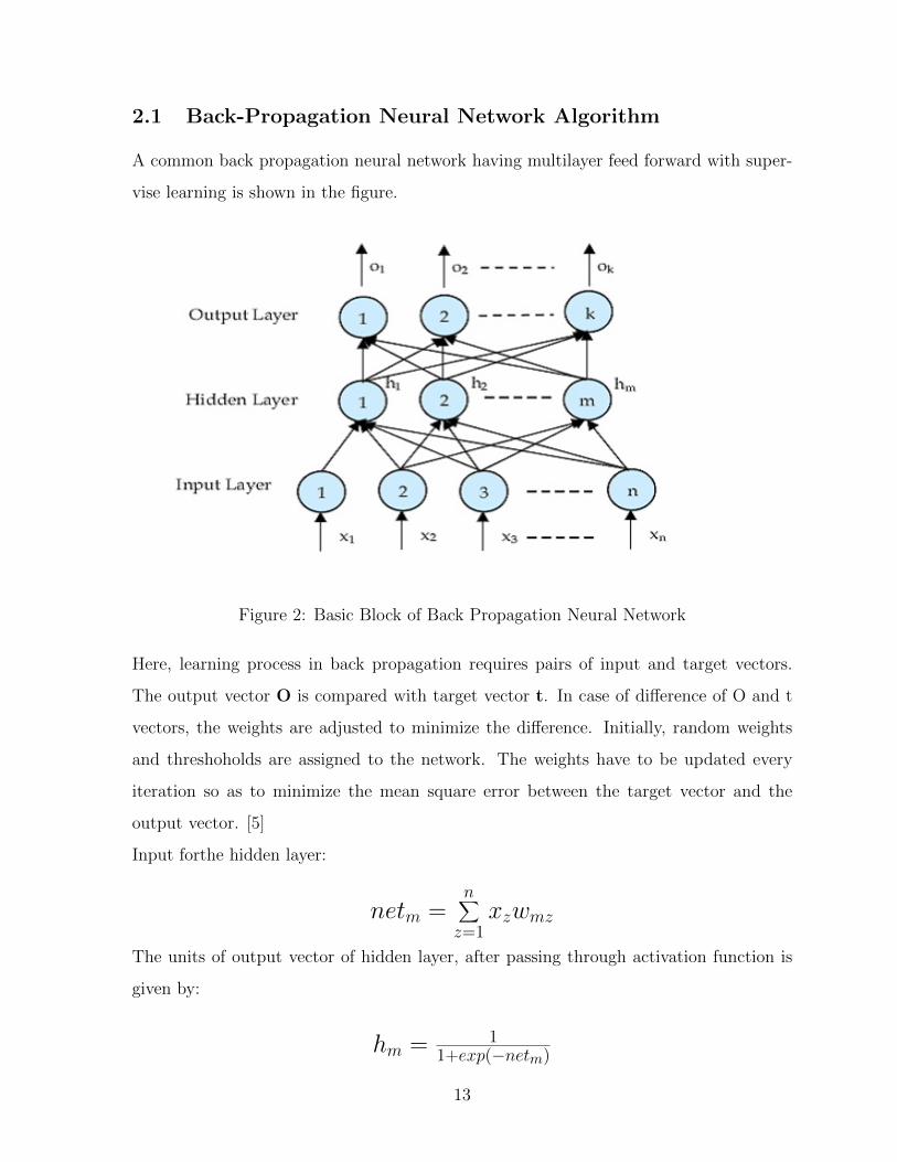
2.1 Back-Propagation Neural Network Algorithm
A common back propagation neural network having multilayer feed forward with super-
vise learning is shown in the figure.
Figure 2: Basic Block of Back Propagation Neural Network
Here, learning process in back propagation requires pairs of input and target vectors.
The output vector O is compared with target vector t. In case of difference of O and t
vectors, the weights are adjusted to minimize the difference. Initially, random weights
and threshoholds are assigned to the network. The weights have to be updated every
iteration so as to minimize the mean square error between the target vector and the
output vector. [5]
Input forthe hidden layer:
netm =n∑z=1
xzwmz
The units of output vector of hidden layer, after passing through activation function is
given by:
hm = 11+exp(−netm)
13

Similarly, the output layer′s input is given by
netk =m∑z=1
hzwkz
The units of the output vector of the output layer is given by
ok = 11+exp(−netk)
For updating the weights, erro needs to be calculated. This is done by:
E = 12(
k∑i=l
(oi − ti)2)
oi and ti represents the target output and the real output at a neuron i in the output
layer, respectively. If the error is less than tolerance, predefined limit, training process
will stop, otherwise weights are to be updated. In case of weights betweeen hidden layer
and output layer, the change of weights is given by:
∆wij = αδihj
where α is the training rate coefficient that is restricted between the range [0.01, 1, 0] ,
hajj is the output of neuron j in the hiddenneuron layer and δi can be obtained by:
δi = (ti − oi)(oi)(l − oi)
Similarly, the change of the weights between output layer and the hidden layer is given
by :
∆wij = βδHixj
where β is a training rate coefficient that is restricted to the range [0.01, 1.0] , xj is the
output of neuron j in the input layer, and δHi can be obtained by:
δHi = xi(l − xi)k∑j=1
δiwij
14

xi is the outpu at neuron i in the input layer, and summation term represents the weighted
sum of all δi values corresponding to neurons in output layerthat obtained in the equation.
Post calculating the weights change in all layers, the weights are updated as:
wij(new) = wij(old) + ∆wij
This process is repeated until the error reaches the minimum value.
15

3 Face Recognition using Principal Component
Analysis
An image can be viewed as a vector. Number of components of the vector will be product
of its width and height. So each pixel corresponds to one vector component. The image–
vector transformation can be obtained via simple concatenation i.e. the rows of the
image are placed beside one another. This image space is not an optimal space for face
description. We need to build a face space, which better describes the face. The basis
vector of this space is called the principal components. There is width x height pixels
in image space. So, the dimension of the face–space is lesser than the dimension of the
image–space. The goal of the Principal Component Analysis is to reduce the dimension
of t his image space so that new basis better describes the typical model of the image
space.
These eigenfaces are a set of eigen vectors used in computer vision problem for human
face recognition. This approach of using eigenfaces for recognition was first developed
by Sirovich and Kirby (1987) and further used by Matthew Turk and Alex Pentland in
face recognition and classification. It is considered the first successful example of face
recognition technology. These eigenvectors were derived from covariance matrix of the
high-dimensional vector space of the possible faces of human beings.
The set of eigenfaces can be generated by the process called as the principal component
analysis (PCA) on large set of different human face images. Eigenfaces can be considered
as a set of ”standardized face ingredients”, derived from the statistical analysis of images
of faces. Every human face can be considered as a combination of these standard faces.
Since a person’s face is not stored as a digital photograph, but just as a list of values
(one value for each of the eigenface in the database used), space required to store each
person’s face is much lesser.
The eigenfaces that are being created will appear as dark areas arranged in some specific
pattern. This pattern is how the different features of a particular face are singled out,
evaluated and scored. There is a pattern to evaluate this symmetry, if there is any facial
hair or where hairline is or evaluate the size of the mouth or nose. Other eigenfaces have
16

some patterns that are slightly tougher to identify, and the eigenface may look very little
like a face. This technique is used in creating eigenfaces and face recognition is hence
done using them. This particular technique is also used for handwriting analysis, lip–
reading, voice–recognition, sign–language and hand gestures interpretation and medical
imaging analysis.[7, 9]
3.1 PCA Algorithm
Principal Component Analysis is a mathematical and statistical technique and is useful
in face recognition & image compression. It is a very common technique used for finding
patterns in high dimensioned data. It also highlights the differences and similarities
amongst the dataset. It is also useful for the extraction of set of eigenfaces from the
initial inputted images of human faces. And these eigenfaces can also be recombined in
proper ratio to reconstruct the original face image.
3.1.1 Eigenface Generation
The first step is to prepare the training set of face images. The pictures belonging to the
training set should be taken under similar lighting conditions, and must be normalized
to have the eyes and mouth aligned across all the images. They must also be all resized
to the same resolution. Every image is treated as a single vector, and simply by the
concatenation of the rows of pixels in original image which results in a single row with
r x c elements. It is also assumed that all the images of the training set are stored in a
matrix T, where every row of the matrix is an image of a face.
The average image Av has to be calculated and then subtracted from each original image
in T. Two different training set has been used from the facial database as mentioned in
Section 4. Resolution of all the images is chosen as 291x243 pixels. The set of original
facial images from 1st training set (yale database) has been shown in figure 3.[7, 6]
T is the image matrix of size (M x N).
M= (r.c) this is the dimension of each image.
N=number of images
17

Figure 3: Yale Pics Database
Ti represents ech row vector corresponding to each image.
Average Vector, Av =N∑i=1
Ti
Subtracting the Mean Face, Xi = Ti − Av
3.1.2 Covariance Matrix and EigenVectors
We then calculate the eigenvalues and eigenvectors for the covariance matrix S. Each
eigenvector is having the same dimensionality as the original images, and thus can be
seen as an image itself. These eigenvectors of the covariance matrix are thus known as
eigenfaces. They are the directions in which the images differ from the mean image. Usu-
ally this will be a computationally expensive step, but the practicality of these eigenfaces
roots from the possibility to compute the eigenvectors of S efficiently without computing
S explicitly, as detailed below.
Covariance Matrix, S = 1N
N∑i=1
XiXTi
Eigenvectors ui of S are:
XXTui = λiui
But, the matrix XXT is very large, hence, practically not feasible to
calculate.
Let us consier matrix D = XTX
18

Eigenvectors of matrix D are vi
XTXvi = λivi
X(XTX)vi = Xλivi
S(Xvi = λi(Xvi)) and Sui = λiui Thus, S and D have same eigenvalues
and their eigenvectors are related as
ui = Xvi
The eigenvectors (eigenfaces) with largest associated eigenvalue are kept. The eigenfaces
obtained are as shown in Figure 4.
Figure 4: Eigenaces for Yale Pics
3.1.3 Weighted Vector
Weighted Vector of the facial image represents the component of every eigenface of that
image. Weighted vector w of all the images is then calculated as
w = uTX
and vector space is formed using these weighted vectors of all facial images.
Each weighted vector of a face represents a point in the weighted vector space. Similarly,
for every new image, its corresponding weighted vector is calculated and mapped into
19

this vector space. Face recognition is done by calculating the distance from its nearest
vector using a distance measurement algorithm like Mahalanobis Distance, Eucledian
Distance, etc
3.2 Reconstruction of Original Images
The original facial images can be reconstructed using the eigenfaces and the corresponding
weighted vector of the images. Each Face Image (minus the average/mean face) can be
represented as a linear combination of best k eigenvectors as:
Ti − Av =k∑j=1
wijuj
where u represents eigenvectors and w weighted vectors.
An Example is shown in Figure 5 demonstrating the linear combination of eigenvectors
to form the original image.
Figure 5: Linear Combination of Eigenvectors
The Reconstructed Images of the test faces taken from the yale database have been
reconstructed using above procedure and shown in Figure 7.
3.3 Mahalanobis Distance Algorithm
We can use either of Euclidean distance algorithm or Mahalanobis Distance Algorithm to
compute the distance between weighted vectors. However, Mahalanobis Algorithm gives
better results.
In Euclidean Distance Algorithm distance between two points x and y is calculated as
20

Figure 6: Reconstruction of original faces
D(x, y) =√
(x− y)t(x− y)
Hence, variations along all axes are treated as equally significant.
In Statistical or Mahalanobis Algorithm distance between two points x and y is calculated
as
D(x, y) =√
(x− y)t(x− y)s−1
where S takes into account the variability of each direction component, i.e. component
with high variability should receive less weightage from those having low variability. Next,
when a new image is to be tested for its validitiy, its corresponding weighted vector is
found and mapped into the vector space. The eigenface whose distance is least to the
test–image and the distance valus is lesser than the accepted threshold value, then the
unknown face can be recognised.
21

4 Facial Databases
Two different facial databases have been used from which set of test faces are taken for
implementing the above face recognition algorithms.
Database 1 : Known persons
It consists of a set of 13 coloured images of 13 different known people (1 Image per Per-
son) taken by us under almost same lighting and background conditions. Resolution of
each image is taken as 320x240 pixels.
Figure 7: Known Faces Databse
Databse 2: The Yale Database
It consists of a set of standard 165 black n white images of 15 different people (11 Im-
ages per Person) taken from yale university standard database created by them for use
in facial algorithm. All the images are properly aligned and taken in same and good
lighting and background conditions. Resolution of each image is taken as 320x243 pixels.
11 Images of each person consists of different expressions and lighting effects as follows:
22

• Normal lights
• Centre Light, Left Light, Right Light
• Sad, Happy, Surprised
• Wink, Sleepy, Normal
• Glasses, Without Glasses
source: http : //face− rec.org/databases/ [1]
The Yale Databse sample is as shown.
Figure 8: Yale Database
23

Database 3: The FERET Database, USA The database contains 1564 sets of
images for a total of 14,126 images that includes 1199 individuals. All the images are of
size 290x240. This database was cropped automatically and segregated into sets of 250
female and 250 male faces. [1]
source: http : /face.nist.gov./colorferet/
The FERET database is as shown in Figure–9.
Figure 9: FERET Database
24

Database 4: Animal faces database
This databse was created by obtaining different animal faces and different objects for the
purpose of face classification. The animal faces were mostly obtained from the website
of Washington state University [8] http : //imagedb.vetmed.wsu.edu/. The other animal
faces and objects were obtained from http : //images.google.com/
A sample of the animal faces database is as shown in Figure–10.
Figure 10: Animal Faces Database
25

5 Analysis and Results
5.1 Analysis of Face Classification using Neural Networks
5.1.1 Human-Non human face Classification
Given a set of animal and human faces, we train our system in a way that once a new
image is inputted to the system, it can detect whether the new image is a human face or
not. This was done with the help of Back Propagation algorithm using Neural Networks
as described in section 2.1 .
The training was done using a set of images consisting of 51 non-human faces and 60
human faces (30 males and 30 females). The learning rate coefficient(α) was fixed at
0.5 and the momentum coefficient(η) was 0.76 . The model thus obtained was tuned
repeatedly until the error value was lesser than the tolerance value of 0.01.
Figure 11: Tuning curve: BPNN
26

Also, the number of hidden layer neurons was chosen accordingly so as to get the best
results on the test set of images. In this case, the test case consisted of 35 non-human
images and 40 human faces (20 males and 20 females). The accuracy rate for different
neurons is as shown.
Figure 12: Accuracy Rate : BPNN
For most of the cases, human faces could be recognised 90%+ of the times. The non-
human images which comprised of both animal faces and random non-face images were
identified more than 80%+ of the times always. From the graph, it was concluded that
the ideal number of neurons for the given problem and the train set was 80.
Another training was done using the Yale Database.The training set consisted of 15 im-
ages from the Yale Database and 15 random animal faces. The learning rate coefficient(α)
was fixed at 0.5 and the momentum coefficient(η) was 0.76 . The model thus obtained
27

was tuned repeatedly until the error value was lesser than the tolerance value of 0.01.The
model tuning curve obtained was as shown in Figure 13.
Figure 13: Training Curve BPNN: Yale Database
The test set of images consisted 30 images out of which 15 human faces were the same
person but with different facial expressions and 15 different animal faces. The succes rate
obtained was 100% for all the neuron cases.
28

5.1.2 Gender Classification
Given a set of human faces, our aim was to distinguish them among male and female
categories. For this classification, again back propagation algorithm was used. The
training set consisted of 100 human faces out of which 50 were male and 50 were female
faces. The learning rate coefficient(α) was fixed at 0.5 and the momentum coefficient(η)
was 0.76 . The model thus obtained was tuned repeatedly until the error value was lesser
than the tolerance value of 0.01.
The test set consisted of 50 images out of which 25 were male and 25 were female faces.
The results obtained are shown in the Figure 14.
Figure 14: Gender Classification Results
Female faces were recognised around 75% of the times accurately while the male faces
were recognised around 90% of the times.
29

5.2 Analysis of Face Recognition using Principal Component
Analysis
5.2.1 Analysis on Yale database:
Step 1: Cropping of Images
Initially, all the images were of the size 320x243 where in the images were captured in
front of a white screen. Two different ways were adopted to crop the images and extract
the face out of the images.
Using theConventional Triangularization Approach, we had to click the Left eye, Right
eye and then the lips. The system would then automatically crop the image using these
three coordiantes and the face extracted would contain the face minus the ears and a part
of forehead. All the images cropped using this method are of uniform size of 293x241.
Using the manual cropping method, all the images are cropped manually using the im-
crop crop command of MATLAB. The resultant images contain the entire face. And,
hence, more number of features are extracted using the manual cropping method.
Figure 15: Manual Cropping
Step 2: Image Pre-processing
All the cropped images were then normalized, and images are store in a matrix form
where each row represents an image vector. Next, an average vector is calculated for all
the images and is subtracted from all the image vectors. Next, the covariance matrix is
generated and corresponding eigefaces are generated. The top eigenfaces are chosen for
Figure 16: Conventional Triangularization Approach
30

the further analysis. In our caase, we chose the top 90% of the eigenfaces. Weighted
vector w of all images is calculated representing the appropriate proportion of each eigen-
face.Using these eigenfaces and the mean face, the images are reconstructed to check the
accuracy of the eigenfaces. If the images are reconstructed properly, we can now proceed
to the recognition part.
Figure 17: Plot of Eigenfaces vs corresponding Eigenvalues
Step 3: Recognition of faces:
Next, when a new image is to be tested for its validitiy, its corresponding weighted vector
is found and mapped into the vector space. The eigenface whose distance is least to the
test–image and the distance valus is lesser than the accepted threshold value, then the
unknown face can be recognised.
The system was trained using 15 images captured under normal lighting conditions. The
images were cropped both manually and automatically.Set of Test Images consists of
all the normal expression images and the other expression images are used during the
recognition part. To test the correctness of the algorithm implemented, all the faces were
31

checked for all the possible present facial expressions.
The following is the result obtained for recognition done using the manual cropping.
Except for the images in which lighting conditions varied, 90%+ recognition rate was
achieved for all the facial expression.
Figure 18: Recognition of faces done using Manual Cropping
The result obtained for the recognition done for the images cropped using the Con-
ventional Triangularization Approach is shown graphically in Figure–19.
Figure 19: Recognition of images cropped using Conventional Triangularization Approach
During the recognition for images cropped automatically, the recognition rate declined
32

to a great extent in case of varied lighting conditions. The results also dropped when
the images features were changed to a greater extent, say in the case of surprised and
winking expression.
Figure 20: Comparision of Recognition rates of different Cropping techniques
Overall, the images which were cropped manually contained more features then the ones
cropped otherwise.A comparision on the two sets of images is as follows. The recognition
rates of the image cropped manually were better and a considerable difference in the
results were noted.
Figure 21: Effect of lighting conditions on recognition
Another point worth noticing here is the effect of different lighting conditions. Images
33

in which lighting varied uniformly had a higher percentage of recognition rate than com-
pared to the ones in a which light was projected from right or left sides. Hence, the
besic assumption of the algorithm implemented that the images taken should be under
uniform lighting conditions. Another important neccesity was the clarity of the images
captured. Image-wise analysis for all the eight expressions is as follows.
Figure 22: Image-wise analysis
34

5.2.2 Analysis on Feret Database:
We had a set of 114 distinct faces available to us. Though it was concluded in the previous
section that manual cropping leads to better results, we opted for automatic cropping
of the images. Automatic cropping is the real practical approach which is implented
in reality. The system was trained using 85 distinct images. The image pre-processing
was same as the case of analysis of the yale databse. The system was tested using 40
known/trained images with different facial expression and 10 unknown faces. During the
image recognition phase, the main analysis point was deciding the threshold values. For
this, we tested the accuracy rate of the program for different threshold values starting
from 0.50 to 1.20 with an increment of 0.01. The accuracy of program was determined
using two different parameters:
• FAR: Flase Acceptance Ratio: This rate determines the number of unknown faces
that were falsely accepted during the recognition.
• FRR: False Rejection Ratio: This rate determines the number of known faces that
were falsely rejected during the recognition.The results obtained were as follows.
Figure 23: Feret Analysis: FAR, FRR
A high FAR value poses a serious securtiy threat to the environment. A high FRR
value is undesirable as it poses a lot of hassles for the authorised personnels to use the
35

environment. Hence, for optimum resultsm we should have a low value of both FRR and
FAR.
Success rate is defined as the maximum sum of known face acceptance and the unknown
face rejection rate, or in other words the minimum sum of known face rejection and the
unknown face acceptance. The succes rate graph obtained is as shown in the Figure–24.
Figure 24: Feret Analysis: Success Rates
From the graphs obtained, the maximum success rate is obtained for threshold values
0.82 to 0.89 (sucess rate of 91.5%). At this threshold value, 1 out of 10 unknown images
were falsely accepted and 3 out of 40 known faces were falsely rejected.
36

6 Conclusion
Training of the system is the most important step for any classification and recognition
system. A good and efficient classification algorithm can save a considerable amount
of search space for recognition purposes. The necessary parameters should be carefully
chosen and neural network model be tuned properly for best results for the classification
phase.
The number of features extracted from the training faces directly affect the recognition
rate. It is also very sensitive to lighting conditions and the clarity of the images. Thresh-
old distance values for acceptable recognition of images should be carefully chosen so as
to find a proper balance between the FAR and the FRR.
37

References
[1] http://face[dash]rec[dot]org/databases. Face recognition homepage – databses.
[2] Sunita Kumari and Banshidhar Majhi. Gender classification by principal component
analysis and support vector machine.
[3] Md. Firdaus Hashim Md. Rizon and Puteh Saad. Face recognition using eigenfaces
and neural networks. American Journal of Applied Sciences, November 2006.
[4] Dr. S. Annadura P. Latha, Dr. L Ganesan. Face recognition using neural networks.
Signal Processsing, An international Journal, 3(5).
[5] G A Vijayalakshami Pai S. Rajasekaran. Neural Networks, Fuzzy Logic and Genetic
Algorithms, ISBN 81-203-2186-3, May 2006. PHI.
[6] Lindsay I Smith. A tutorial on principal component analysis, february 2002.
[7] Mathew Turk and Alex Pentland. Eigenfaces for recognition. Journal of cognitive
neuroscience, November 1991, 3.
[8] http://www.imagedb.vetmed.wsu.edu Wahington State University. Image Database
at the College of Veterinary Medicine.
[9] http://en.wikipedia.org/facerecognitionsystem Wikipedia, Face Recognition System.
38