Efficient Distributed Linear Classification Algorithmsvia the Alternating Direction Method of Multipliers

Caoxie Zhang Honglak Lee Kang G. ShinDepartment of EECS

University of MichiganAnn Arbor, MI 48109, USAcaoxiezh@umich.edu

Department of EECSUniversity of Michigan

Ann Arbor, MI 48109, USAhonglak@eecs.umich.edu

Department of EECSUniversity of Michigan

Ann Arbor, MI 48109, USAkgshin@eecs.umich.edu

Abstract

Linear classification has demonstrated suc-cess in many areas of applications. Modernalgorithms for linear classification can trainreasonably good models while going throughthe data in only tens of rounds. However,large data often does not fit in the memory ofa single machine, which makes the bottleneckin large-scale learning the disk I/O, not theCPU. Following this observation, Yu et al.(2010) made significant progress in reducingdisk usage, and their algorithms now outper-form LIBLINEAR. In this paper, rather thanoptimizing algorithms on a single machine,we propose and implement distributed algo-rithms that achieve parallel disk loading andaccess the disk only once. Our large-scalelearning algorithms are based on the frame-work of alternating direction methods of mul-tipliers. The framework derives a subproblemthat remains to be solved efficiently for whichwe propose using dual coordinate descent andtrust region Newton method. Our experi-mental evaluations on large datasets demon-strate that the proposed algorithms achievesignificant speedup over the classifier pro-posed by Yu et al. running on a single ma-chine. Our algorithms are faster than exist-ing distributed solvers, such as Zinkevich etal. (2010)’s parallel stochastic gradient de-scent and Vowpal Wabbit.

1 IntroductionLarge-scale linear classification has proven successfulin many areas, such as machine learning, data min-ing, computer vision, and security. With the burgeon-ing of social media, which provides an unprecedentedamount of user-provided supervised information, therewill likely be more extreme-scale data requiring classi-fication. Training on these large data can be done on

Appearing in Proceedings of the 15th International Con-ference on Artificial Intelligence and Statistics (AISTATS)2012, La Palma, Canary Islands. Volume XX of JMLR:W&CP XX. Copyright 2012 by the authors.

a single machine or a distributed system. Many algo-rithms for a single machine, such as LIBLINEAR [6]and PEGASOS [16], have been developed and exten-sively used in both academia and industry. These al-gorithms can sequentially train on the entire data in afew tens of rounds to obtain a good model and utilizethe sparsity of the data. However, training with large-scale data on a single machine becomes slow becauseof the disk I/O, not the CPU. Since the disk band-width is 2-3 orders of magnitude slower than mem-ory bandwidth and CPU speed, much of the trainingphase is spent on loading data rather than process-ing. This scenario worsens when the data cannot fit inmain memory, causing severe disk swaps. Yu et al. [19]addressed this problem by reading blocks of data andprocessing them in batches. Their algorithm reducedthe disk I/O time via pre-fetching and achieved a sig-nificant speedup over the original LIBLINEAR, whichis one of the state-of-art libraries for linear classifica-tion [6]. However, since all single-machine algorithmsgo through the entire data many times, they have toload the same data from the disk multiple times whenthe data cannot fit in memory. If the data requiresmore than tens of gigabytes of storage (greater thanthe typical RAM capacity), those algorithms are stillinefficient since the disk needs to be accessed morethan once and the training takes hours to complete.

On the other hand, distributed systems composed ofcommercial servers (nodes) are becoming more preva-lent both in research labs and medium-scale compa-nies. A large Internet company may have thousands ofnodes. Algorithms running on distributed systems cannow load the data in parallel to the distributed mem-ory and train without using disk any more, thereby sig-nificantly reducing the cumbersome disk loading time.One important challenge in the field is to design newalgorithms in the parallel setting, since the current lin-ear classification algorithms are inherently sequential.

In this paper, we propose distributed algorithms forlinear classification. The system architecture is illus-trated in Fig. 1. We use the alternating directionmethod of multipliers (ADMM) as the framework forsolving distributed convex optimization; see Boyd etal. [2] for a review of ADMM. This framework intro-duces additional variables to regularize the difference

1398

Caoxie Zhang, Honglak Lee, Kang G. Shin

Data x𝐵𝑚

# of features

Solving subproblems in parallel

Aggregation and broadcasting

Data x𝐵1

Data x𝐵2

𝐰 + 𝐮 𝐳

Data distributed in machines

x𝐵1, z w1, u1

x𝐵𝑚, 𝐳 𝐰𝑚, 𝐮𝑚

x𝐵2, z w2, u2

⋮ ⋮

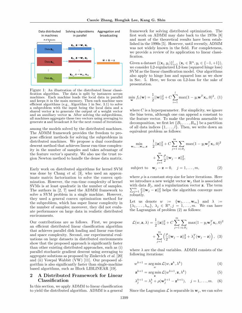
Figure 1: An illustration of the distributed linear classi-fication algorithm. The data is split by instances acrossmachines. Each machine loads the local data in paralleland keeps it in the main memory. Then each machine usesefficient algorithms (e.g., Algorithm 1 in Sec. 3.1) to solvea subproblem with the input being the local data and ashared vector z to generate the output of a weight vectorand an auxiliary vector u. After solving the subproblems,all machines aggregate these two vectors using averaging togenerate z and broadcast it for the next round of iterations.

among the models solved by the distributed machines.The ADMM framework provides the freedom to pro-pose efficient methods for solving the subproblems indistributed machines. We propose a dual coordinatedescent method that achieves linear run-time complex-ity in the number of samples and takes advantage ofthe feature vector’s sparsity. We also use the trust re-gion Newton method to handle the dense data matrix.

Early work on distributed algorithms for kernel SVMwas done by Chang et al. [3], who used an approx-imate matrix factorization to solve the convex opti-mization. However, the run-time complexity of kernelSVMs is at least quadratic in the number of samples.The authors in [2, 7] used the ADMM framework tosolve a SVM problem in a single machine. However,they used a general convex optimization method forthe subproblem, which has super linear complexity inthe number of samples; moreover, they did not evalu-ate performance on large data in realistic distributedenvironments.

Our contributions are as follows. First, we proposean efficient distributed linear classification algorithmthat achieves parallel disk loading and linear run-timeand space complexity. Second, our experimental eval-uations on large datasets in distributed environmentsshow that the proposed approach is significantly fasterthan other existing distributed approaches, such as (i)parallel stochastic gradient descent using averaging toaggregate solutions as proposed by Zinkevich et al. [20]and (ii) Vowpal Wabbit (VW) [11]. Our proposed al-gorithm is also significantly faster than single-machinebased algorithms, such as Block LIBLINEAR [19].

2 A Distributed Framework for LinearClassification

In this section, we apply ADMM to linear classificationto yield the distributed algorithm. ADMM is a general

framework for solving distributed optimization. Thefirst work on ADMM may date back to the 1970s [8]and most of the theoretical results have been estab-lished in the 1990s [5]. However, until recently, ADMMwas not widely known in the field. For completeness,we provide a review of its application to linear classi-fication.

Given a dataset {(xi, yi)}li=1 (xi ∈ Rn, yi ∈ {−1,+1}),we consider L2-regularized L2-loss (squared hinge loss)SVM as the linear classification model. Our algorithmsalso apply to hinge loss and squared loss as we showin Sec. 5. Here, we focus on L2-loss for the sake ofpresentation.

minw

f1(w) =1

2||w||22 + C

l∑

i=1

max(1− yiwTxi, 0)2, (1)

where C is a hyperparameter. For simplicity, we ignorethe bias term, although one can append a constant tothe feature vector. To make the problem amenable todecomposition, we first let {B1, . . . , Bm} be a partitionof all data indices {1, . . . , l}. Then, we write down anequivalent problem as follows:

minw1,...,wm,z

1

2||z||22 + C

m∑

j=1

∑

i∈Bj

max(1− yiwTj xi, 0)2

+

m∑

j=1

ρ

2||wj − z||22,

subject to wj − z = 0, j = 1, . . . ,m, (2)

where ρ is a constant step size for later iterations. Herewe introduce a new weight vector wj that is associatedwith data Bj , and a regularization vector z. The term∑mj=1

ρ2 ||wj − z||22 helps the algorithm converge more

robustly.

Let us denote w := {w1, . . . ,wm} and λ :={λ1, . . . , λm}, λj ∈ Rn, j = 1, . . . ,m. We can havethe Lagrangian of problem (2) as follows:

L(w, z, λ) =1

2||z||22 + C

m∑

j=1

∑

i∈Bj

max(1− yiwTj xi, 0)2

+m∑

j=1

(ρ2||wj − z||22 + λTj (wj − z)

), (3)

where λ are the dual variables. ADMM consists of thefollowing iterations:

wk+1 = arg minw

L(w, zk, λk) (4)

zk+1 = arg minzL(wk+1, z, λk) (5)

λk+1j = λkj + ρ(wk+1

j − zk+1), j = 1, . . . ,m. (6)

Since the Lagrangian L is separable in wj , we can solve

1399

Caoxie Zhang, Honglak Lee, Kang G. Shin

problem (4) in parallel:

wk+1j = arg min

w′C∑

i∈Bj

max(1− yiw′Txi, 0)2 (7)

+ρ

2||w′ − z||22 + λTj (w′ − z), j = 1, ...,m.

Also, zk+1 has a closed form solution:

zk+1 =ρ∑mj=1 wk+1

j +∑mj=1 λ

kj

mρ+ 1. (8)

A simple change of variables, letting λj = ρuj , canmake the quadratic form of wj in Eq. (8) more com-pact. We now have the new ADMM iterations as:

wk+1j = arg min

wC∑

i∈Bj

max(1− yiwTxi, 0)2 (9)

+ρ

2||w− zk + ukj ||22, j = 1, . . . ,m.

zk+1 =

∑mj=1

(wk+1j + ukj

)

m+ 1/ρ(10)

uk+1j = ukj + wk+1

j − zk+1, j = 1, . . . ,m. (11)

Here, each machine j solves the subproblem (9) in par-

allel, which is only associated with data xBj , {xi :i ∈ Bj}. Machine j also loads the data xBj

from thedisk only once and stores them in the memory in theADMM iterations. Each machine only needs to com-municate wj and uj without passing the data.

The ADMM iterations also give the following theoret-ical guarantees. For any ρ > 0 we have:

1. If we define the residual variable rk = [wk1 −

zk, . . . ,wkm − zk], then rk → 0 as k →∞.

2. The objective function in problem (2) convergesto the optimal objective function of problem (1).

To show the above, since 12 ||z||22 and max(1 −

yiwTxi, 0)2 are both closed and proper convex func-

tions and problem (1) possesses strong duality, theymeet the conditions to guarantee the convergence re-sults [2]. These results imply that eventually wk

j would

agree upon a consensus vector zk, which would con-verge to the solution of the original SVM problem (1).The auxiliary variables ukj convey to machine j how

different its wkj is from zk and serve as the signal to

pull wk+1j into consensus when machine j solves the

subproblem (9).

ADMM is essentially a subgradient-based method thatsolves the dual problem of (2). However, it has abetter convergence result as compared to other dis-tributed approaches, such as the dual decompositionmethod [2]. ADMM is a first order method, so it wouldseem that it would take many iterations to achieve

high accuracy; however, our empirical experience sug-gests that ADMM usually takes only tens of itera-tions to achieve good accuracy. This few number ofthe iterations can be enough for large-scale classifica-tion tasks since the SVM (or logistic regression) usesloss functions that approximate the misclassificationerrors, and it may not be necessary to minimize theseobjectives exactly [1, 17]. In our experiments, we showthat our algorithm achieves fast convergence in train-ing optimality and test accuracy within only a few tensof ADMM iterations for large-scale datasets.

3 Efficient Algorithms for Solving theSubproblem

Although ADMM provides a parallel framework, theissue of solving the subproblem (9) efficiently still re-mains. In this subproblem, each machine containsa portion of the data, which can still be quite largeto solve. In this section, we present both a dualmethod and a primal method. The dual method isa coordinate descent method similar to the one in[9]. To obtain an ε-optimal dual solution, our methodhas a computational complexity of O(nnz log(1/ε)),where nnz is the total number of non-zero featuresin the data. For well-scaled data, the term log(1/ε)(including the constant) usually becomes a few oftens to achieve good accuracy, namely, the algorithmonly needs to sequentially pass the data in a fewof tens rounds. The primal method is a trust re-gion Newton method similar to the one in [12]. Thismethod obtains an approximated Hessian using theconjugate gradient. The computational complexityis O(nnz × number of conjugate gradient iterations×number of Newton iterations). The primal methodcan be more efficient if the data matrix is dense. Wefirst detail the dual coordinate descent method andthen briefly describe the trust region Newton method.

3.1 A Dual Coordinate Descent Method

We rewrite the subproblem (9) in a more readable way:

minw

f2(w) =ρ

2||w− v||22 + C

s∑

i=1

max(1− yiwTxi, 0)2,

(12)

where v = zk − ukj at the k-th ADMM iterations, and{x1, . . . ,xs} denotes the data in xBj for some machinej. The above problem is different from traditionalSVM in its regularization term, which also considersthe consensus to other machines’ solutions. Therefore,we still need an efficient special solver for this problem.

The dual problem of (12) can be written as a quadraticprogramming:

minα

f3(α) =1

2ραT Qα− bTα

subject to αi ≥ 0, ∀i, (13)

where Q = Q + D, Qij = yiyjxTi xj , D is a diagonal

matrix, Dii = ρ/(2C) and b = [1 − y1vTx1, . . . , 1 −ysv

Txs]T .

1400

Caoxie Zhang, Honglak Lee, Kang G. Shin

We solve this problem using dual coordinate descent,which optimizes one variable in α at a time and thencircularly moves to the next variable and so on. Forproblem (13), the one-variable optimization has a closeform solution since it is a quadratic minimization. Inother words, for any i, we can optimize αi while fixing

other variables. Let G(t)i be the partial derivative of f3

with respect of αi at the t-th iteration, then we have

G(t)i =

s∑

j=1

α(t)j Qij − bi. (14)

Thus, the optimal αi will be the root of G(t)i projected

on [0,∞). We can update αi as

α(t+1)i = max

(bi −

∑j 6=i α

(t)j Qij

Qii, 0

)

= max(α(t)i −G

(t)i /Qii, 0

)(15)

We can also use the projected partial derivative, de-

noted as PG(t)i , to determine the stopping criteria of

coordinate descent:

PG(t)i =

{min(0, G

(t)i ) if α

(t)i = 0,

G(t)i otherwise.

(16)

If PG(t)i = 0, we do not need to update α

(t)i .

To get G(t)i in Eq. (14), the main computation is O(s).

However, due to the special structure of the problem,we can reduce to O(n), where n is the average numberof non-zero features in the data, to make the computa-tional complexity independent of the size of the data,s. The key idea here is to maintain an intermediatevector w(t) at each iteration as

w(t) =

s∑

j=1

yjα(t)j xj + v. (17)

Then, we can express G(t)i as

G(t)i = yiw

(t)Txi − 1 +Diiα(t)i (18)

The main computation is then the dot product of w(t)

and xi, which is O(n) if we save xi as a sparse form. To

maintain w(t) after α(t)i changes to α

(t+1)i , we update

it as follows:

w(t+1) = w(t) +(α(t+1)i − α(t)

i

)yixi. (19)

This operation also takes O(n). The overall procedureis provided in Algorithm 1.

For theoretical results, we can easily apply results in[13] to show that Algorithm 1 converges and it takesO(log(1/ε)) iterations of while-loops to achieve an ε-accurate solution, i.e., f3(α) ≤ f3(α∗) + ε. There-fore, the total computation is O(sn log(1/ε)) for anε-accurate solution, where sn is the total number ofnon-zero features in data xBj

.

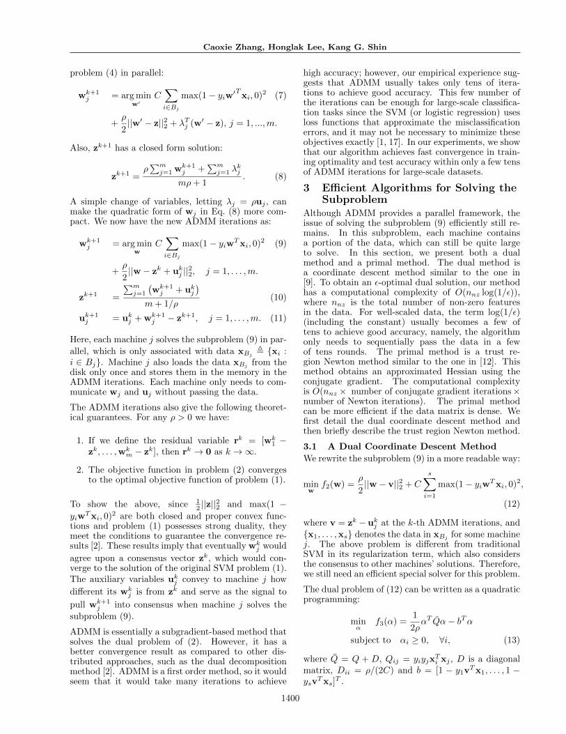
Algorithm 1 A dual coordinate descent method forsolving the problem (12)

Initialize α(0), w(0) =∑si=1 yiα

(0)i xi + v and t = 0.

while α(t) is not optimal dofor i = 1 . . . s dot = t+ 1

G(t)i = yiw

(t)Txi − 1 +Diiα(t)i

PG(t)i =

{min(0, G

(t)i ) if α

(t)i = 0,

G(t)i otherwise.

if |PG(t)i | 6= 0 then

α(t+1)i = max

(α(t)i −G

(t)i /Qii, 0

)

w(t+1) = w(t) +(α(t+1)i − α(t)

i

)yixi

elseα(t+1) = α(t)

w(t+1) = w(t)

end ifend for

end while

3.2 A Trust Region Newton Method

We use the trust region Newton method in [12] to solvethe problem (12). Since the Hessian in L2 loss SVMdoes not exist, the authors in [12] used a generalizedHessian for approximation. With the generalized Hes-sian they use the conjugate gradient method to find theNewton-like direction and use the trust region Newtonmethod to iterate. The method is general and can bedirectly applied to our problem (12). The only impor-tant difference is the gradient of the objective function:

∇f2(w) = (ρ+ 2C∑

i∈Ixix

Ti )w− 2C

∑

i∈Iyixi − ρv, (20)

where I = {i|(1− yiw(t)xi) > 0}.4 Improving the Distributed

AlgorithmsWe have discussed the use of two efficient methodsto solve the subproblem (9) under the framework ofADMM. However, there is still room for further im-provement of the distributed algorithms. In this sec-tion, we describe several simple but important tech-niques that can significantly affect efficiency.

Random permutation of data. Since each machineprocesses only a portion of the data and communi-cates its solutions to other machines, if the local datacontains mostly the same label, it may take a largenumber of ADMM iterations to achieve consensus. Auseful technique is to randomly shuffle the data to dif-ferent machines to ensure that class labels in the dataare balanced. This technique reduces ADMM’s totalnumber of iterations.

Warm start in solving subproblem (9). In solvingsubproblem (9), it is not necessary to start from somefixed (e.g., zero) vector. In particular, wk

j may notchange much at the very end of the ADMM iterations.

1401

Caoxie Zhang, Honglak Lee, Kang G. Shin

So, we use wk−1 as the starting point for obtainingwk. Specifically, in Algorithm 1 we save the previousα used for obtaining wk−1 and reuse it as α0. Forthe primal method, we can directly use wk−1 as thestarting point for Newton iteration. This techniqueshortens the time within each ADMM iteration.

Inexact minimization (early stopping) of sub-problem (9). Solving (9) exactly, especially at theinitial ADMM iterations, may not be worthwhile sincethe exact solutions usually require a large amount oftime and might not be the direction for achieving goodconsensus. In fact, the problem (9) can be solved ap-proximately. In Algorithm 1, we can limit the while-loop’s maximum number of iterations to be, for exam-ple, M times. This corresponds to going through thelocal data only M rounds. In the trust region Newtonmethod, we can limit the number of Newton iterations.This technique can dramatically speed up the ADMMiterations.

Over-relaxation. wk+1j is used for updating z and

u in (10)–(11). In fact, wk+1j can be added with the

previous value of zk to improve convergence. The new

wk+1j in (10)-(11) can be written as:

wk+1j = βwk+1

j + (1− β)zk. (21)

We used β ∈ [1.5, 1.8], as reported in [4]. This tech-nique can reduce the total number of ADMM itera-tions while achieving the same accuracy.

5 ImplementationsOur algorithms are simple and easy to implement ondistributed systems. First, we consider their imple-mentations from a data perspective. The data is splituniformly by data instances for processing on differentmachines. At the start, each machine loads its owndata in parallel to fit in its RAM. Data in memory isrepresented as a sparse matrix, so the space complex-ity is O(|Bj |n) for machine j. Each machine j main-tains its own wj and uj in its memory and processesthem in w-update and u-update in (9, 11) in parallel

with other machines. Machine j broadcasts wk+1j +ukj

and waits to collect∑mj=1(wk+1

j + ukj ) for z-update in

(10). For the communication of wk+1j + ukj , and syn-

chronization, i.e., waiting to collect∑mj=1(wk+1

j +ukj ),

we use the Message-Passing Interface (MPI) [14] forinter-machine coordination, which is one of the mostpopular parallel programming frameworks for scientificapplications. MPI supports high-level message com-munication and eliminates most of the programmingburdens for low-level synchronization.

Second, we also implement our algorithms for differ-ent loss functions such as hinge loss and square loss.These loss functions would yield different forms of sub-problem (9). However, we can apply the same ideaof dual coordinate descent to solving the subproblemsince it is still a quadratic programming and allowsus to use the sparsity trick of Eq. (17). We imple-mented all the algorithms, e.g., ADMM and subprob-

lem solvers, in C/C++. Specifically, we use OpenMPIfor the communication in ADMM, and also modify theLIBLINEAR library for solving the problem (9) usingthe dual and primal methods. To further improve theimplementations, we also used the following additionaltechniques.

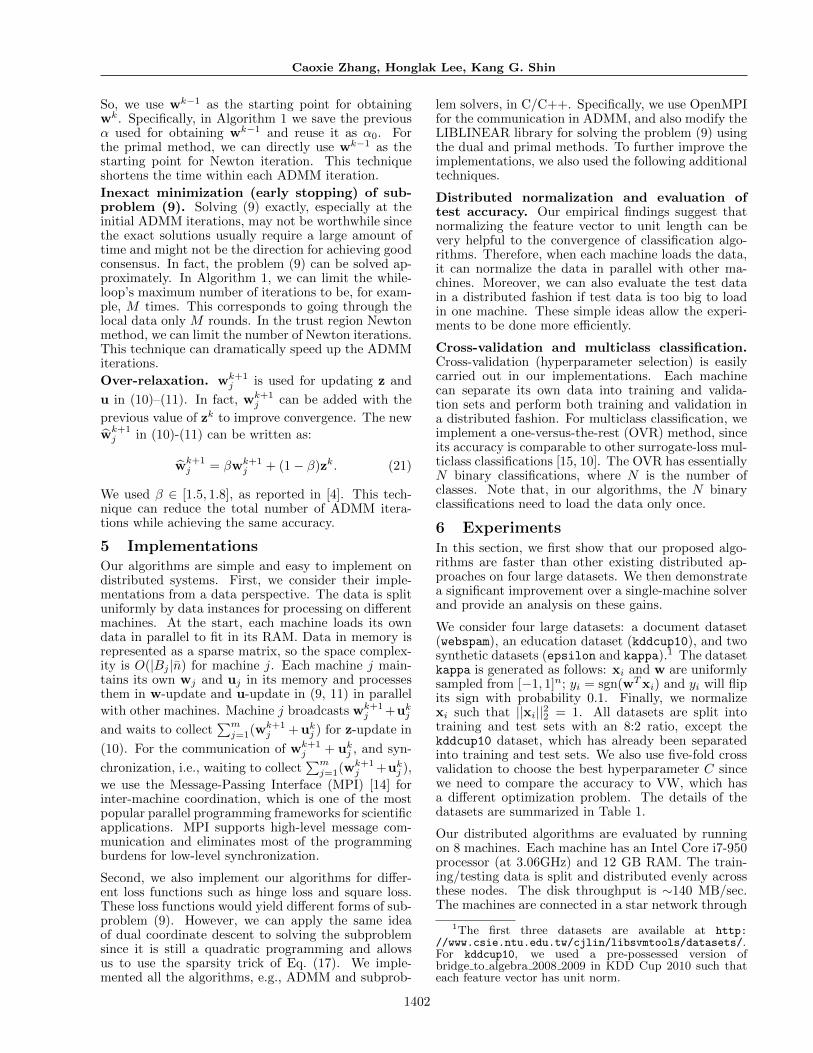
Distributed normalization and evaluation oftest accuracy. Our empirical findings suggest thatnormalizing the feature vector to unit length can bevery helpful to the convergence of classification algo-rithms. Therefore, when each machine loads the data,it can normalize the data in parallel with other ma-chines. Moreover, we can also evaluate the test datain a distributed fashion if test data is too big to loadin one machine. These simple ideas allow the experi-ments to be done more efficiently.

Cross-validation and multiclass classification.Cross-validation (hyperparameter selection) is easilycarried out in our implementations. Each machinecan separate its own data into training and valida-tion sets and perform both training and validation ina distributed fashion. For multiclass classification, weimplement a one-versus-the-rest (OVR) method, sinceits accuracy is comparable to other surrogate-loss mul-ticlass classifications [15, 10]. The OVR has essentiallyN binary classifications, where N is the number ofclasses. Note that, in our algorithms, the N binaryclassifications need to load the data only once.

6 ExperimentsIn this section, we first show that our proposed algo-rithms are faster than other existing distributed ap-proaches on four large datasets. We then demonstratea significant improvement over a single-machine solverand provide an analysis on these gains.

We consider four large datasets: a document dataset(webspam), an education dataset (kddcup10), and twosynthetic datasets (epsilon and kappa).1 The datasetkappa is generated as follows: xi and w are uniformlysampled from [−1, 1]n; yi = sgn(wTxi) and yi will flipits sign with probability 0.1. Finally, we normalizexi such that ||xi||22 = 1. All datasets are split intotraining and test sets with an 8:2 ratio, except thekddcup10 dataset, which has already been separatedinto training and test sets. We also use five-fold crossvalidation to choose the best hyperparameter C sincewe need to compare the accuracy to VW, which hasa different optimization problem. The details of thedatasets are summarized in Table 1.

Our distributed algorithms are evaluated by runningon 8 machines. Each machine has an Intel Core i7-950processor (at 3.06GHz) and 12 GB RAM. The train-ing/testing data is split and distributed evenly acrossthese nodes. The disk throughput is ∼140 MB/sec.The machines are connected in a star network through

1The first three datasets are available at http://www.csie.ntu.edu.tw/cjlin/libsvmtools/datasets/.For kddcup10, we used a pre-possessed version ofbridge to algebra 2008 2009 in KDD Cup 2010 such thateach feature vector has unit norm.

1402

Caoxie Zhang, Honglak Lee, Kang G. Shin

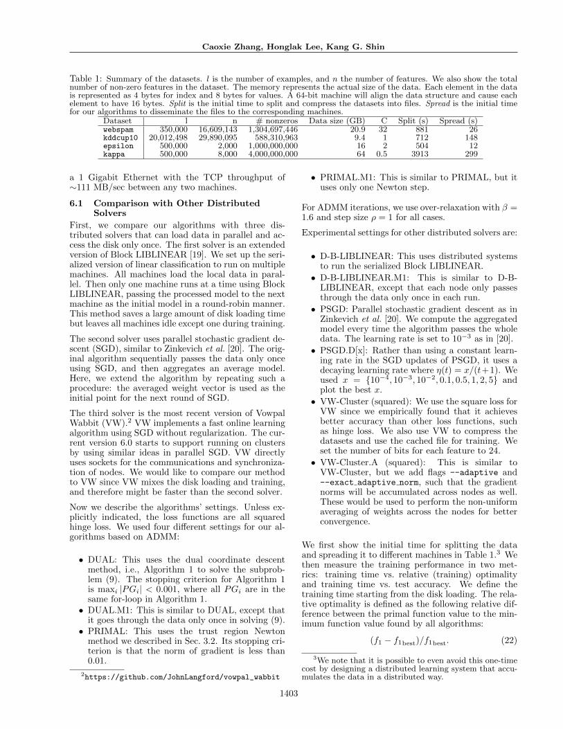
Table 1: Summary of the datasets. l is the number of examples, and n the number of features. We also show the totalnumber of non-zero features in the dataset. The memory represents the actual size of the data. Each element in the datais represented as 4 bytes for index and 8 bytes for values. A 64-bit machine will align the data structure and cause eachelement to have 16 bytes. Split is the initial time to split and compress the datasets into files. Spread is the initial timefor our algorithms to disseminate the files to the corresponding machines.

Dataset l n # nonzeros Data size (GB) C Split (s) Spread (s)webspam 350,000 16,609,143 1,304,697,446 20.9 32 881 26kddcup10 20,012,498 29,890,095 588,310,963 9.4 1 712 148epsilon 500,000 2,000 1,000,000,000 16 2 504 12kappa 500,000 8,000 4,000,000,000 64 0.5 3913 299

a 1 Gigabit Ethernet with the TCP throughput of∼111 MB/sec between any two machines.

6.1 Comparison with Other DistributedSolvers

First, we compare our algorithms with three dis-tributed solvers that can load data in parallel and ac-cess the disk only once. The first solver is an extendedversion of Block LIBLINEAR [19]. We set up the seri-alized version of linear classification to run on multiplemachines. All machines load the local data in paral-lel. Then only one machine runs at a time using BlockLIBLINEAR, passing the processed model to the nextmachine as the initial model in a round-robin manner.This method saves a large amount of disk loading timebut leaves all machines idle except one during training.

The second solver uses parallel stochastic gradient de-scent (SGD), similar to Zinkevich et al. [20]. The orig-inal algorithm sequentially passes the data only onceusing SGD, and then aggregates an average model.Here, we extend the algorithm by repeating such aprocedure: the averaged weight vector is used as theinitial point for the next round of SGD.

The third solver is the most recent version of VowpalWabbit (VW).2 VW implements a fast online learningalgorithm using SGD without regularization. The cur-rent version 6.0 starts to support running on clustersby using similar ideas in parallel SGD. VW directlyuses sockets for the communications and synchroniza-tion of nodes. We would like to compare our methodto VW since VW mixes the disk loading and training,and therefore might be faster than the second solver.

Now we describe the algorithms’ settings. Unless ex-plicitly indicated, the loss functions are all squaredhinge loss. We used four different settings for our al-gorithms based on ADMM:

• DUAL: This uses the dual coordinate descentmethod, i.e., Algorithm 1 to solve the subprob-lem (9). The stopping criterion for Algorithm 1is maxi |PGi| < 0.001, where all PGi are in thesame for-loop in Algorithm 1.

• DUAL.M1: This is similar to DUAL, except thatit goes through the data only once in solving (9).

• PRIMAL: This uses the trust region Newtonmethod we described in Sec. 3.2. Its stopping cri-terion is that the norm of gradient is less than0.01.

2https://github.com/JohnLangford/vowpal_wabbit

• PRIMAL.M1: This is similar to PRIMAL, but ituses only one Newton step.

For ADMM iterations, we use over-relaxation with β =1.6 and step size ρ = 1 for all cases.

Experimental settings for other distributed solvers are:

• D-B-LIBLINEAR: This uses distributed systemsto run the serialized Block LIBLINEAR.

• D-B-LIBLINEAR.M1: This is similar to D-B-LIBLINEAR, except that each node only passesthrough the data only once in each run.

• PSGD: Parallel stochastic gradient descent as inZinkevich et al. [20]. We compute the aggregatedmodel every time the algorithm passes the wholedata. The learning rate is set to 10−3 as in [20].

• PSGD.D[x]: Rather than using a constant learn-ing rate in the SGD updates of PSGD, it uses adecaying learning rate where η(t) = x/(t+1). Weused x = {10−4, 10−3, 10−2, 0.1, 0.5, 1, 2, 5} andplot the best x.

• VW-Cluster (squared): We use the square loss forVW since we empirically found that it achievesbetter accuracy than other loss functions, suchas hinge loss. We also use VW to compress thedatasets and use the cached file for training. Weset the number of bits for each feature to 24.

• VW-Cluster.A (squared): This is similar toVW-Cluster, but we add flags --adaptive and--exact adaptive norm, such that the gradientnorms will be accumulated across nodes as well.These would be used to perform the non-uniformaveraging of weights across the nodes for betterconvergence.

We first show the initial time for splitting the dataand spreading it to different machines in Table 1.3 Wethen measure the training performance in two met-rics: training time vs. relative (training) optimalityand training time vs. test accuracy. We define thetraining time starting from the disk loading. The rela-tive optimality is defined as the following relative dif-ference between the primal function value to the min-imum function value found by all algorithms:

(f1 − f1best)/f1best. (22)

3We note that it is possible to even avoid this one-timecost by designing a distributed learning system that accu-mulates the data in a distributed way.

1403

Caoxie Zhang, Honglak Lee, Kang G. Shin

We also compare the difference between current testaccuracy and best accuracy (acc∗%) over time, using

acc∗%− acc%. (23)

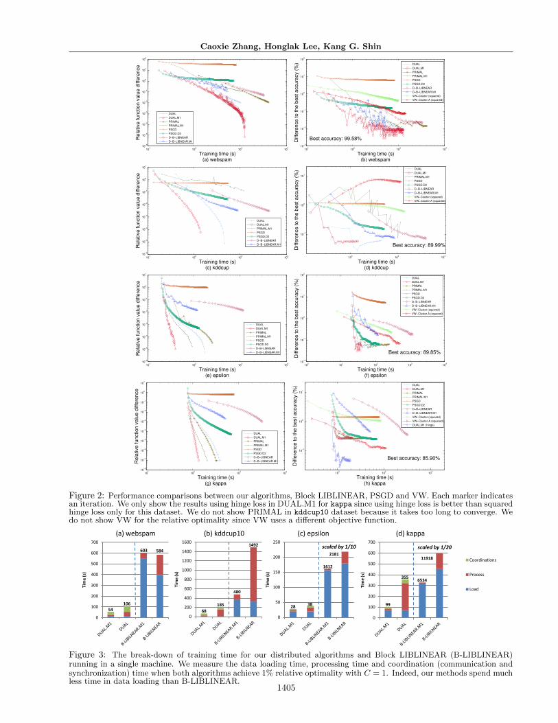
All distributed solvers enjoy the benefit of loading inparallel only once from disk, which alleviates the cum-bersome disk loading. Here, we are interested in whichapproach can converge quickly both in primal objec-tive and test accuracy. As shown in the left columnof Fig. 2, DUAL.M1 has the fastest convergence ratein reducing primal function value. Interestingly, eventhough DUAL.M1 goes through data only once whensolving the subproblem (9), ADMM still improves inmost of the iterations despite this inexact minimiza-tion. Using the exact minimization, such as DUALand PRIMAL, does not yield much less primal func-tion value and takes a longer time. PSGD*4, de-spite our significant efforts of tuning the learning rate,cannot reach 1% relative optimality in a reasonableamount of time for the sparse datasets webspam andkddcup. PSGD* also has a slower convergence rate inthe dense datasets epsilon and kappa. We conjecturethat PSGD* is slower because it does not have aux-iliary variables (e.g., u as in ADMM) to convey thedifferences in local models that can more strongly pulltoward the consensus. D-B-LIBLINEAR* is slower be-cause it does not use parallel training thus leaving mostmachines unutilized.

As the right column of Fig. 2 shows, DUAL.M1 (usingsquared hinge loss) is the fastest method to achievethe best accuracy in datasets webspam, kddcup andepsilon, while DUAL.M1 using hinge loss outper-forms others in the kappa dataset. We show DUAL.M1using hinge loss in the kappa dataset because it yieldsbetter accuracy than squared hinge loss, though notin the rest of the datasets. Note that VW does notsupport squared hinge loss, but does support otherloss functions, such as squared loss and hinge loss.We found that VW using squared loss is much bet-ter than hinge loss, and therefore, we show the bestresults of VW in the figures. Since the objective func-tion is different, VW is not directly comparable toDUAL*, PRIMAL*, PSGD*, and D-B-LIBLINEAR*.VW-Cluster.A is faster than VW-Cluster (except fordataset kddcup) because it uses non-uniform averag-ing to improve convergence. However, the non-uniformaveraging still yields slower convergence of VW thanour algorithms. In summary, these results suggest thatour proposed optimization methods converge faster intest accuracy with a proper choice of loss function.

6.2 Comparison to a Single-machine Solver.Now, we study how our distributed algorithms com-pare against Block LIBLINEAR running in a singlemachine in terms of training time. We denote thesingle-machine solver using Block LIBLINEAR as B-LIBLINEAR and its variant that passes the data onlyonce in each block as B-LIBLINEAR.M1. See Fig. 3for the break-down of training time. Although Block

4“*” means the wildcard character. Here PSGD* standsfor PSGD and PSGD.D[x].

LIBLINEAR attempts to reduce the time spent indisk, the disk loading time still occupies a significantportion since Block LIBLINER would load the samesamples from disk multiple times. We also observethat both DUAL.M1 and B-LIBLINEAR.M1 spendmuch less time in processing data than loading, andthat they are more efficient than those that use ex-act minimization, such as DUAL and B-LIBLINEAR.These findings reveal that, in large-scale classification,the main component in the training time is data load-ing, which motivated us to improve it by using a dis-tributed system for parallel loading. In addition toperforming parallel disk loading only once, our al-gorithms introduce coordinations between machines,such as communications and synchronization. Com-munications involve the passing of wj + uj at eachADMM iteration, and synchronization corresponds tothe waiting time to collect this message. For relativelymodest dimensional features such as in epsilon andkappa, the coordination overhead is quite small. Fordatasets that have high dimensional features, such aswebspam and kddcup10, the coordination time turnsout to be greater than the processing time. Over-all, DUAL.M1 achieves 7 ∼ 60 fold speedup over B-LIBLINEAR or B-LIBLINEAR.M1.

7 Discussions and ConclusionExtremely high-dimensional data, e.g., having morethan billions of features, would create significant over-heads for our distributed algorithms to communicatedue to the network bandwidth constraint. One solu-tion for this is to use the hash trick [18] to randomlygroup different features to reduce the dimension andtherefore alleviate communication overheads.

We evaluated and performed experiments on 8 ma-chines, a typical scale in academia or research labs. Itwould be interesting to evaluate in a kilo-node scaleas in a data center. In such settings, coordinationsbetween nodes will need to be carefully designed whencalculating average; for example, nodes in the samerack can aggregate the sums and then communicateacross the racks. Our current implementation requiresthat the data be fit in the distributed memory to en-sure fast training. If the data is larger than the dis-tributed memory, it is straightforward to apply theidea of Block LIBLINEAR to load and train a portionof data in batch when solving the subproblems.

In this paper, we proposed simple and efficient dis-tributed algorithms for large-scale linear classification.Our algorithms provide a significant performance gainover state-of-the-art linear classifiers running in a sin-gle machine and existing state-of-the-art distributedsolvers, which shows the promise of our approach inlarge-scale learning problems. Our code is availableat: http://eecs.umich.edu/~caoxiezh/.

AcknowledgmentsThis work was supported in part by a Google Fac-ulty Research Award and AFOSR Grant FA9550-10-1-0393.

1404

Caoxie Zhang, Honglak Lee, Kang G. Shin

101

102

103

104

10−6

10−5

10−4

10−3

10−2

10−1

100

101

102

Training time (s)(a) webspam

Re

lative

fu

nctio

n v

alu

e d

iffe

ren

ce

DUAL

DUAL.M1

PRIMAL

PRIMAL.M1

PSGD

PSGD.D2

D−B−LIBNEAR

D−B−LIBNEAR.M1

101

102

103

104

10−3

10−2

10−1

100

101

102

Training time (s)(b) webspam

Diffe

ren

ce

to

th

e b

est

accu

racy (

%)

Best accuracy: 99.58%

DUAL

DUAL.M1

PRIMAL

PRIMAL.M1

PSGD

PSGD.D2

D−B−LIBNEAR

D−B−LIBNEAR.M1

VW−Cluster (squared)

VW−Cluster.A (squared)

101

102

103

104

10−6

10−5

10−4

10−3

10−2

10−1

100

101

Training time (s)(c) kddcup

Re

lative

fu

nctio

n v

alu

e d

iffe

ren

ce

DUAL

DUAL.M1

PRIMAL.M1

PSGD

PSGD.D2

D−B−LIBNEAR

D−B−LIBNEAR.M1

102

103

104

10−1

100

101

Training time (s)(d) kddcup

Diffe

rence to the b

est accura

cy (

%)

Best accuracy: 89.99%

DUAL

DUAL.M1

PRIMAL.M1

PSGD

PSGD.D2

D−B−LIBNEAR

D−B−LIBNEAR.M1

VW−Cluster (squared)

VW−Cluster.A (squared)

101

102

103

104

10−6

10−5

10−4

10−3

10−2

10−1

100

101

Training time (s)(e) epsilon

Re

lative

fu

nctio

n v

alu

e d

iffe

ren

ce

DUAL

DUAL.M1

PRIMAL

PRIMAL.M1

PSGD

PSGD.D2

D−B−LIBNEAR

D−B−LIBNEAR.M1

100

101

102

103

104

10−2

10−1

100

101

102

Training time (s)(f) epsilon

Diffe

ren

ce

to

th

e b

est

accu

racy (

%)

Best accuracy: 89.85%

DUAL

DUAL.M1

PRIMAL

PRIMAL.M1

PSGD

PSGD.D2

D−B−LIBNEAR

D−B−LIBNEAR.M1

VW−Cluster (squared)

VW−Cluster.A (squared)

101

102

103

104

10−8

10−7

10−6

10−5

10−4

10−3

10−2

10−1

100

101

Training time (s)(g) kappa

Re

lative

fu

nctio

n v

alu

e d

iffe

ren

ce

DUAL

DUAL.M1

PRIMAL

PRIMAL.M1

PSGD

PSGD.D2

D−B−LIBNEAR

D−B−LIBNEAR.M1

102

103

104

10−1

100

101

Training time (s)(h) kappa

Diffe

rence to the b

est accura

cy (

%)

Best accuracy: 85.90%

DUAL

DUAL.M1

PRIMAL

PRIMAL.M1

PSGD

PSGD.D2

D−B−LIBNEAR

D−B−LIBNEAR.M1

VW−Cluster (squared)

VW−Cluster.A (squared)

DUAL.M1 (hinge)

Figure 2: Performance comparisons between our algorithms, Block LIBLINEAR, PSGD and VW. Each marker indicatesan iteration. We only show the results using hinge loss in DUAL.M1 for kappa since using hinge loss is better than squaredhinge loss only for this dataset. We do not show PRIMAL in kddcup10 dataset because it takes too long to converge. Wedo not show VW for the relative optimality since VW uses a different objective function.

0

100

200

300

400

500

600

700

Tim

e (s

)

scaled by 1/20

11918

0

100

200

300

400

500

600

700

Tim

e (s

)

0

200

400

600

800

1000

1200

1400

1600

Tim

e (s

)

0

50

100

150

200

250

Tim

e (s

)

scaled by 1/10

2181

(a) webspam (b) kddcup10 (c) epsilon (d) kappa

Coordinations

Process

Load

54 106

603 584

68 28 38 99

355

185

480

1492

1612

6534

Figure 3: The break-down of training time for our distributed algorithms and Block LIBLINEAR (B-LIBLINEAR)running in a single machine. We measure the data loading time, processing time and coordination (communication andsynchronization) time when both algorithms achieve 1% relative optimality with C = 1. Indeed, our methods spend muchless time in data loading than B-LIBLINEAR.

1405

Caoxie Zhang, Honglak Lee, Kang G. Shin

References

[1] L. Bottou and Y. LeCun. Large scale online learn-ing. In Advances in Neural Information Process-ing Systems, 2004.

[2] S. Boyd, N. Parikh, E. Chu, B. Peleato, andJ. Eckstein. Distributed optimization and statis-tical learning via the alternating direction methodof multipliers. 3(1):1–122, 2011.

[3] E. Y. Chang, K. Zhu, H. Wang, and H. Bai.PSVM: Parallelizing support vector machines ondistributed computers. In Advances in Neural In-formation Processing Systems, 2008.

[4] J. Eckstein. Parallel alternating direction multi-plier decomposition of convex programs. Jour-nal of Optimization Theory and Applications,80(1):39–62, 1994.

[5] J. Eckstein and D. P. Bertsekas. On thedouglas-rachford splitting method and the proxi-mal point algorithm for maximal monotone opera-tors. Mathematical Programming, 55(1):293–318,1992.

[6] R.-E. Fan, K.-W. Chang, C.-J. Hsieh, X.-R.Wang, and C.-J. Lin. LIBLINEAR: A libraryfor large linear classification. Journal of MachineLearning Research, 9:1871–1874, 2008.

[7] P. A. Forero, A. Cano, and G. B. Giannakis.Consensus-based distributed support vector ma-chines. Journal of Machine Learning Research,11:1663–1707, 2010.

[8] D. Gabay and B. Mercier. A dual algorithmfor the solution of nonlinear variational problemsvia finite element approximation. Computers andMathematics with Applications, 2(1):17–40, 1976.

[9] C.-J. Hsieh, K.-W. Chang, C.-J. Lin, S. S.Keerthi, and S. Sundararajan. A dual coordinatedescent method for large-scale linear SVM. InProceedings of the 25th International Conferenceon Machine Learning, 2008.

[10] S. S. Keerthi, S. Sundararajan, K.-W. Chang,C.-J. Hsieh, and C.-J. Lin. A sequential dualmethod for large scale multi-class linear svms. InProceedings of the 14th ACM SIGKDD Interna-tional Conference on Knowledge Discovery andData Mining, 2008.

[11] J. Langford, L. Li, and A. Strehl. Vowpal Wabbitonline learning project. Technical report, 2007.

[12] C.-J. Lin, R. C. Weng, and S. S. Keerthi. Trustregion Newton method for large-scale logistic re-gression. Journal of Machine Learning Research,9:627–650, 2008.

[13] Z. Q. Luo and P. Tseng. On the convergence ofthe coordinate descent method for convex differ-entiable minimization. Journal of OptimizationTheory and Applications, 72:7–35, 1992.

[14] MPI Forum. MPI: A Message-Passing InterfaceStandard, version 2.2, 2009.

[15] R. Rifkin and A. Klautau. In defense of one-vs-all classification. Journal of Machine LearningResearch, 5:101–141, 2004.

[16] S. Shalev-Shwartz, Y. Singer, and N. Srebro. Pe-gasos: Primal estimated sub-gradient solver forSVM. In Proceedings of the 24th InternationalConference on Machine Learning, 2007.

[17] S. Shalev-Shwartz and N. Srebro. SVM optimiza-tion: inverse dependence on training set size. InProceedings of the 25th international Conferenceon Machine Learning, pages 928–935, 2008.

[18] Q. Shi, J. Petterson, G. Dror, J. Langford,A. Smola, and S. Vishwanathan. Hash kernelsfor structured data. Journal of Machine LearningResearch, 10:2615–2637, 2009.

[19] H.-F. Yu, C.-J. Hsieh, K.-W. Chang, and C.-J.Lin. Large linear classification when data cannotfit in memory. In Proceedings of the 16th ACMSIGKDD International Conference on KnowledgeDiscovery and Data Mining, 2010.

[20] M. Zinkevich, A. J. Smola, M. Weimer, and L. Li.Parallelized stochastic gradient descent. In Ad-vances in Neural Information Processing Systems,2010.

1406