chapter 2 classi cation - purdue university · 2019-02-17 · chapter 2 classi cation in this...

Chapter 2

Classification

In this chapter we study one of the most basic topics in machine learning called classi-fication. By classification we meant a supervised learning procedure where we try toclassify a sample based on a model learned from the data in a training dataset. The goalof this chapter is to understand the general principle of classification, to explore variousmethodologies so that we can do classification, and to make connections between differentmethods.

2.1 Discriminant Function

Basic Terminologies

A classification method always starts with a pair of variables (x, y). The first variablex ∈ X ⊂ Rd is an input vector. The set X is called the input space. Depending onthe application, an input could the intensity of a pixel, a wavelet coefficient, the phaseangle of wave, or anything we want to model. We assume that each input vector has adimensionality d and d is finite. The second variable y ∈ {1, . . . , k} = Y denotes the classlabel of the classes {C1, . . . , Ck}. The choice of the class labels is arbitrary. They do notneed to be positive integers. For example, in binary classification, one can choose y ∈ {0, 1}or y ∈ {−1,+1}, depending which one is more convenient mathematically.

In supervised learning, we assume that we have a training set D. A training set is acollection of paired variables (xj, yj), for j = 1, . . . , n. The vector xj denotes the j-th sampleinput in D, and yj denotes the corresponding class label. The relationship between xj andyj is specified by the target function f : X → Y such that yj = f(xj). The target functionis unknown. By unknown we really mean that it is unknown.

The training set D can be generated deterministically or probabilistically. If D is deter-ministic, then {xj}nj=1 is a sequence of fixed vectors. If D is probabilistic, then there is anunderlying generative model that generates {(xj)}nj=1. The generative model is specified bythe distribution pX(x). The distinction between a deterministic and a probabilistic model is

1

Figure 2.1: Visualizing a training data D consisting of two classes C1 and C2, with each class being a multi-dimensional Gaussian. The gray dots represent the samples outside the training set, whereas the color dotsrepresent the samples inside the training set.

subtle but important. We will go into the details when we study learning theory in Chapter4. For now, let us assume that xj’s are generated probabilistically.

When there is no noise in creating the labels, the class label yj is defined as yj = f(xj).However, in the presence of noise, instead of using a fixed but unknown target function f togenerate yj = f(xj), we assume that yj is drawn from a posterior distribution y ∼ pY |X(y|x).As a result, the training pair (xj, yj) is now drawn according to the joint distributionpX,Y (x, y) of random variables X and Y . By Bayes Theorem, it holds that pX,Y (x, y) =pY |X(y|x)pX(x), which means the joint distribution pX,Y (x, y) can be completely determinedby the posterior distribution pY |X(y|x) and the data generator pX(x).

Example. [Gaussian]. Consider a training set D consisting of training samples {(xj, yj)}.The input vector xj is a d-dimensional vector in R2, and the label yj is either {1, 2}. Thetarget function f is a mapping which assigns each xj to a correct yj. The left hand side ofFigure 2.1 shows a labeled dataset, marking the data points in red and blue.

We assume that for each class, the input vectors are distributed according to a d-dimensional Gaussian:

pX |Y (x | i) =1√

(2π)d|Σi|exp

{−1

2(x− µi)TΣ−1i (x− µi)

}, (2.1)

where µi ∈ Rd is the mean vector, and Σi ∈ Rd×d is the covariance matrix. If we assumethat pY (i) = πi for i = 1, 2, then the joint distribution of X and Y is defined through theBayes Theorem

pX,Y (x, i) = pX|Y (x|i)pY (i)

= πi ·1√

(2π)d|Σi|exp

{−1


}.

In the above example, we can use a simple MATLAB / Python code to visualize the joint

c© 2018 Stanley Chan. All Rights Reserved. 2

distribution. Here, the proportion of class 1 is π = 0.25, and the proportion of class 2 is1−π = 0.75. When constructing the data, we define two random variables Y ∼ Bernoulli(π),and X with conditional distribution X|Y ∼ N (µY ,ΣY ). Therefore, the actual randomnumber is drawn by a two-step procedure: First draw Y from a Bernoulli. If Y = 1, thendraw X from the first Gaussian; If Y = 0, then draw X from the other Gaussian.

mu1 = [0 0];

mu0 = [2 0];

Sigma1 = [.25 .3; .3 1];

Sigma0 = [0.5 0.1; 0.1 0.3];

n = 1000; % number of samples

p = 0.25; % pi

y = (rand(n,1)<=p); % class label

idx1 = (y==1); % indices of class 1

idx0 = (y==0); % indices of class 0

x = mvnrnd(mu1, Sigma1, n).*repmat(y,[1,2]) + ...

+ mvnrnd(mu0, Sigma0, n).*repmat((1-y),[1,2]);

The plotting of the data points can be done by a scatter plot. In the code below, we use theindices idx1 and idx0 to identify the class 1 and class 0 data points. This is an aftermathlabel. When x was first generated, it was unlabeled. Therefore, in an unsupervised learningcase, there will not be any coloring of the dots.

figure(1);

scatter(x(idx1,1),x(idx1,2),’rx’, ’LineWidth’, 1.5); hold on;

scatter(x(idx0,1),x(idx0,2),’bo’, ’LineWidth’, 1.5); hold off;

xlabel(’x’); ylabel(’y’);

set(gcf, ’Position’, [100, 100, 600, 300]);

The result of this example is shown in Figure 2.2. If we count of the number of red andblue markers, we see that there are approximately 25% red and 75% blue. This is a resultof the prior distribution. Shown in this plot is a linearly not separable example, meaningthat some data points will never be classified correctly by a linear classifier even if we usethe classifier is theoretically optimal.

One thing we need to be careful in the above example is that the training samples{(xj, yj)}nj=1 represent a finite set of n samples drawn from the distribution pX,Y (x, y).The distribution pX,Y (x, y) is “bigger” in the sense that many samples in pX,Y (x, y) arenot necessarily part of D. Think about doing a survey in the United States about a per-son’s height: The distribution pX,Y (x, y) covers the entire population, whereas D is only asub-collection of the data resulting from the survey. Samples that are inside the trainingset are called the in-samples, and samples that are outside the training set are called theout-samples. See Figure 2.1 for an illustration.


-2 -1 0 1 2 3 4 5

-3

-2

-1

0

1

2

3

Figure 2.2: Generating random samples from two Gaussians where the class label is generated according toa Bernoulli distribution.

The difference between in-sample and out-sample is important. Straightly speaking, theGaussian parameters (µ1,Σ1) in the previous example are called the population parameter,and they are unknown no matter how many people we have surveyed unless we have askedeveryone. Given the training set D, any model parameter estimated from D is the sampleparameter (µ̂1, Σ̂1).

Given the training dataset D, the goal of learning (in particular classification) is to picka mapping h : X → Y that can minimize the error of misclassification. The mapping h iscalled a hypothesis function. A hypothesis function could be linear, nonlinear, convex,non-convex, expressible as equations, or an algorithm like a deep neural network. The setcontaining all candidate hypothesis functions is called the hypothesis set H . See Figure 2.3for an illustration.

Figure 2.3: Hypothesis set H and hypothesis function h. The goal of learning is to use an algorithm to finda hypothesis function or approximate a hypothesis function such that the error of classification is minimized.In this example, h2 is a better hypothesis because it has a lower misclassification rate.

So what is “error” in classification? To be clear about this, we are fundamentally askingtwo questions (i) How well does the hypothesis function h do for the training dataset, i.e.,


the in-samples? (ii) How well does it generalize to the testing dataset, i.e., the out-samples? A good hypothesis function should minimize the error for both. If a hypothesisfunction that only performs well for the training set but generalizes poorly to the testingdataset, then it is more or less useless as it can only memorize the pattern but not predictthe pattern.

We will come back to the details of these fundamental questions later. For now, we willpresent a set of computational tools for seeking (or approximating) a hypothesis function.The methods we are presenting here are by no means exhaustive, but they all fall into thesame general principle of linear classification.

Linear Discriminant Analysis

The goal of classification is to construct a good hypothesis function h. In this course wewill focus on linear classifiers under a framework called linear discriminant analysis. Whyare we interested in linear classifiers? First, linear classifiers are easy to understand. Theyhave simple geometry, and they often allow analytic results. Second, linear classifiers containmost of the essential insight we need to understand a classification method, and the principleis generalizable to nonlinear classifiers.

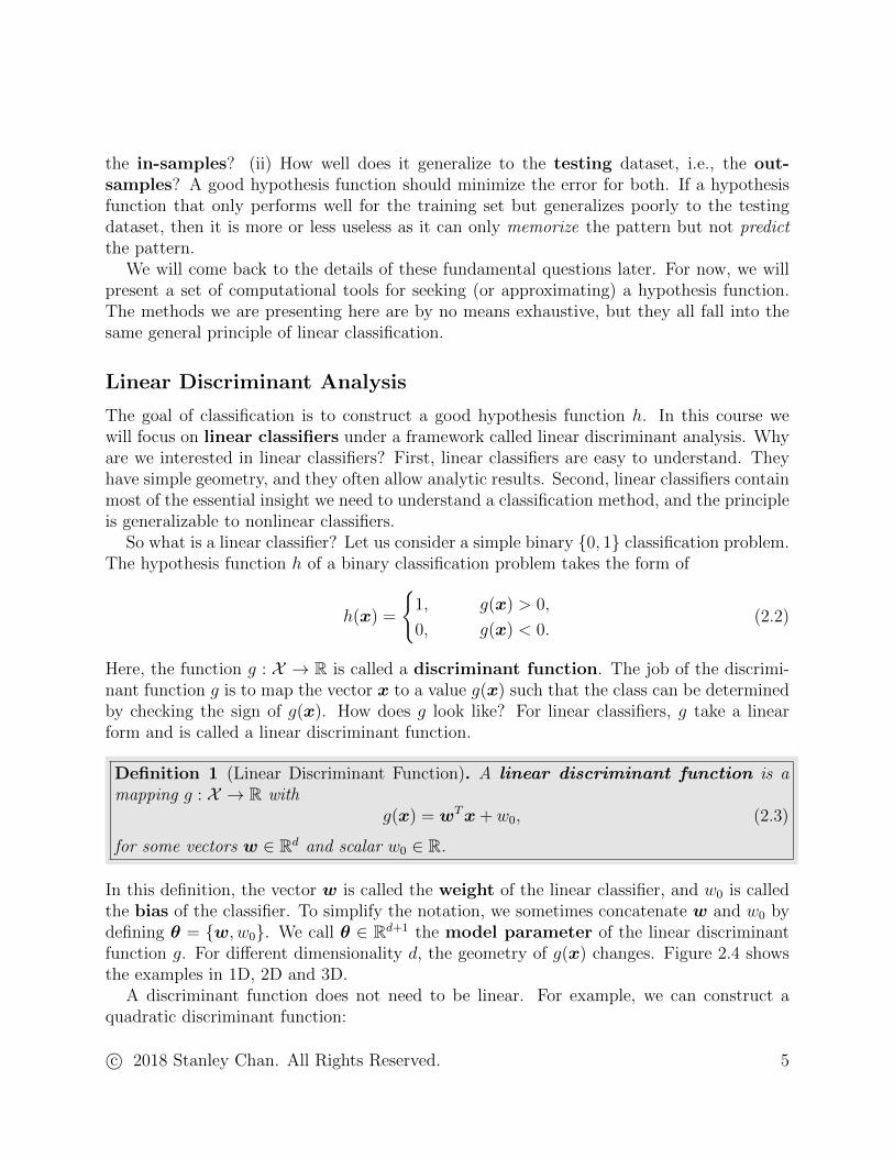
So what is a linear classifier? Let us consider a simple binary {0, 1} classification problem.The hypothesis function h of a binary classification problem takes the form of

h(x) =

{1, g(x) > 0,

0, g(x) < 0.(2.2)

Here, the function g : X → R is called a discriminant function. The job of the discrimi-nant function g is to map the vector x to a value g(x) such that the class can be determinedby checking the sign of g(x). How does g look like? For linear classifiers, g take a linearform and is called a linear discriminant function.

Definition 1 (Linear Discriminant Function). A linear discriminant function is amapping g : X → R with

g(x) = wTx+ w0, (2.3)

for some vectors w ∈ Rd and scalar w0 ∈ R.

In this definition, the vector w is called the weight of the linear classifier, and w0 is calledthe bias of the classifier. To simplify the notation, we sometimes concatenate w and w0 bydefining θ = {w, w0}. We call θ ∈ Rd+1 the model parameter of the linear discriminantfunction g. For different dimensionality d, the geometry of g(x) changes. Figure 2.4 showsthe examples in 1D, 2D and 3D.

A discriminant function does not need to be linear. For example, we can construct aquadratic discriminant function:


Figure 2.4: Discriminant function g(x) at different dimensions. [Left] In 1D, the discriminant function issimply a cutoff value. [Middle] In 2D, the discriminant function is a line. [Right] In 3D, the discriminantfunction is a plane.

Definition 2 (Quadratic Discriminant Function). A quadratic discriminant functionis a mapping g : X → R with

g(x) =1

2xTWx+wTx+ w0, (2.4)

for some matrix W ∈ Rd×d, some vector w ∈ Rd and some scalar w0 ∈ R.

In quadratic discriminant function, the model parameter is θ = {W ,w, w0}. Dependingon W , the geometry of g could be convex, concave, or neither. Figure 2.5 below shows aquadratic discriminant function separating an inner and an outer cluster of data points.

Figure 2.5: A quadratic discriminant function is able to classify data using quadratic surfaces. This exampleshows an ellipsoid surface for separating an inner and outer cluster of data points.

Beyond quadratic discriminant function, another common approach of constructing dis-criminant functions is the method of transformation. We shall come back to this idea laterin this chapter. For now, let us focus on linear discriminant functions.


Geometry of Linear Discriminant Function

The equation g(x) = 0 defines a hyperplane where on one side of the plane we have C1 andon the other side of the plane we have C2. The geometry is summarized below.

Theorem 1 (Geometry of a linear discriminant function). Let g be a linear discriminantfunction, and let H = {x | g(x) = 0} be the separating hyperplane. Then,

(i) w/‖w‖2 is the normal vector of H, i.e., for any x1,x2 ∈ H, we have

wT (x1 − x2) = 0. (2.5)

(ii) For any x0, the distance between x0 and H is

d(x0,H) = g(x0)/‖w‖2. (2.6)

Proof. To prove the first statement, we note consider two points x1 ∈ H and x2 ∈ H.Since both points are on the hyperplane, we have g(x1) = 0 and g(x2) = 0, and hencewTx1 +w0 = wTx2 +w0 = 0. Rearranging the equations yields wT (x1−x2) = 0. Thereforew is a normal vector to the surface H, and w/‖w‖2 is a scaled version of w so that thenorm of w/‖w‖2 is 1.

To prove the second statement, we can decompose x0 as x0 = xp + η w‖w‖2 , where xp is

the orthogonal projection of x0 onto H such that g(xp) = 0. In other words, we decomposex0 into its two orthogonal components: one along the normal vector w, and the other alongthe tangent. Since

g(x0) = wTx0 + w0 = wT

(xp + η

w

‖w‖2

)+ w0

= g(xp) + η‖w‖2 = η‖w‖2,

we have that η = g(x0)/‖w‖2.

(a) Geometry (b) Decision

Figure 2.6: The geometry of linear discriminant function.


Exercise 1.1. An alternative proof of the above result is to solve an optimization. Showthat the solution to the problem

minimizex

‖x− x0‖2 subject to wTx+ w0 = 0, (2.7)

is given by

x = x0 −g(x0)

‖w‖2· w

‖w‖2. (2.8)

Hint: Use Lagrange multiplier.

The geometry of the above theorem is illustrated in Figure 2.6. The theorem tells us twothings about the hyperplane: (i) Orientation of H. The orientation of H is specified byw/‖w‖2, as it is the normal vector of H. (ii) Distance to H. The distance of a point x0

to H is g(x0)/‖w‖2. Therefore, the bigger the value g(x0) is, the farther away the point x0

is from the decision boundary, and hence the more “confident” x0 is belonging to one classbut not the other. To classify a data point x, we check whether x belongs to C1 or C2 bychecking if g(x) > 0.

Separating Hyperplane Theorem

Before we move on to talk about different methods to construct the discriminant function g,we should ask a “learnability” question: For what kind of datasets can we guarantee that alinear classifier is able to perfectly classify the data? This is a universal result because thecertificate derived from answering this question has to hold for any linear classifier and anyalgorithms used to train the classifier.

Theorem 2 (Separating Hyperplane Theorem). Let C1 and C2 be two closed convex setssuch that C1 ∩ C2 = ∅. Then, there exists a linear function

g(x) = wTx+ w0,

such that g(x) > 0 for all x ∈ C1 and g(y) < 0 for all y ∈ C2.

Pictorially, the separating hyperplane says that if C1 and C2 are convex and do not overlap,then there must exists two points x∗ ∈ C1 and y∗ ∈ C2 such that ‖x∗ − y∗‖2 represents theshortest distance between the two sets. The vector w = x∗ − y∗ is therefore a potentialcandidate for the normal of the separating hyperplane. The potential candidate for w0 isthen −wT

(x∗+y∗

2

), i.e., the mid point of x∗ and y∗. Once w and w0 are identified, we can

check the inner product of any x ∈ C1 with w, i.e., wTx+w0, and check its sign. This givesthe proof of the theorem.


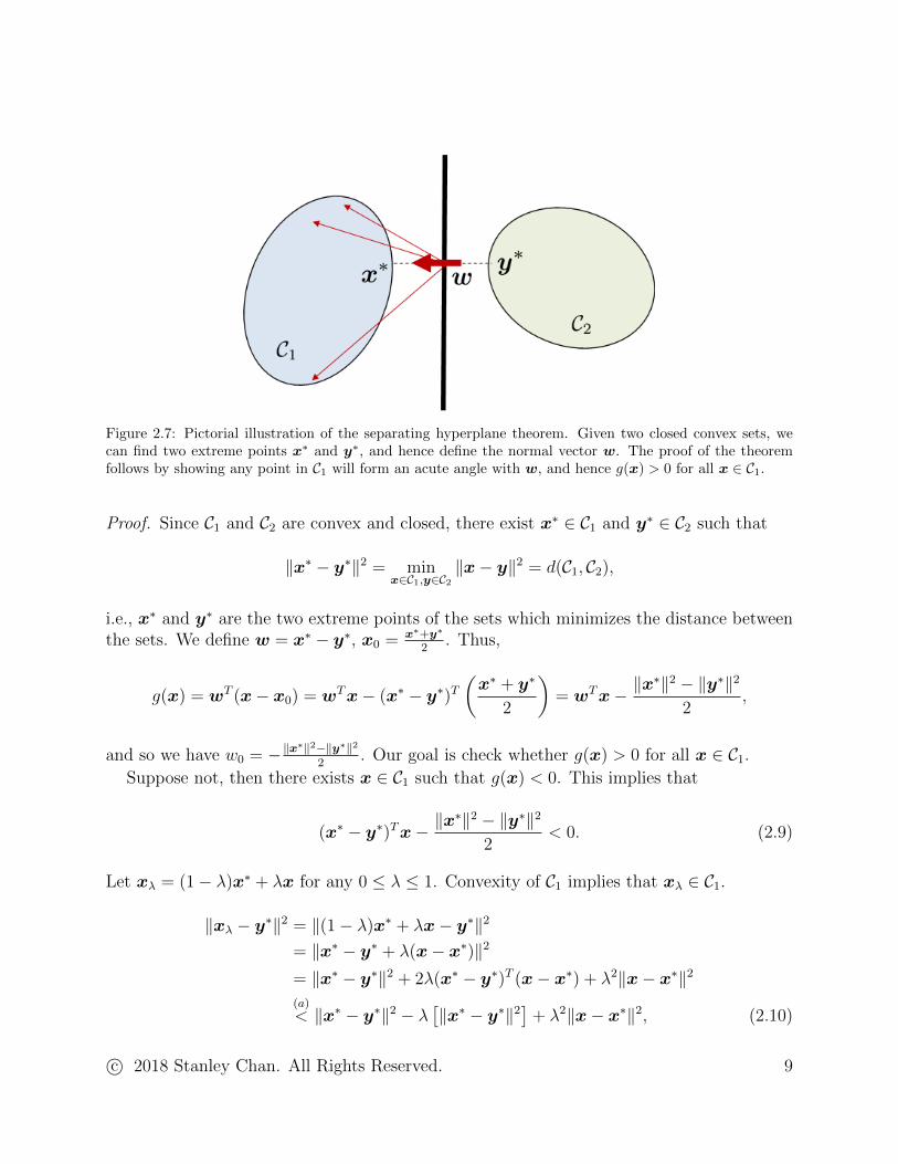
Figure 2.7: Pictorial illustration of the separating hyperplane theorem. Given two closed convex sets, wecan find two extreme points x∗ and y∗, and hence define the normal vector w. The proof of the theoremfollows by showing any point in C1 will form an acute angle with w, and hence g(x) > 0 for all x ∈ C1.

Proof. Since C1 and C2 are convex and closed, there exist x∗ ∈ C1 and y∗ ∈ C2 such that

‖x∗ − y∗‖2 = minx∈C1,y∈C2

‖x− y‖2 = d(C1, C2),

i.e., x∗ and y∗ are the two extreme points of the sets which minimizes the distance betweenthe sets. We define w = x∗ − y∗, x0 = x∗+y∗

2. Thus,

g(x) = wT (x− x0) = wTx− (x∗ − y∗)T(x∗ + y∗

2

)= wTx− ‖x

∗‖2 − ‖y∗‖2

2,

and so we have w0 = −‖x∗‖2−‖y∗‖2

2. Our goal is check whether g(x) > 0 for all x ∈ C1.

Suppose not, then there exists x ∈ C1 such that g(x) < 0. This implies that

(x∗ − y∗)Tx− ‖x∗‖2 − ‖y∗‖2

2< 0. (2.9)

Let xλ = (1− λ)x∗ + λx for any 0 ≤ λ ≤ 1. Convexity of C1 implies that xλ ∈ C1.

‖xλ − y∗‖2 = ‖(1− λ)x∗ + λx− y∗‖2

= ‖x∗ − y∗ + λ(x− x∗)‖2

= ‖x∗ − y∗‖2 + 2λ(x∗ − y∗)T (x− x∗) + λ2‖x− x∗‖2

(a)< ‖x∗ − y∗‖2 − λ

[‖x∗ − y∗‖2

]+ λ2‖x− x∗‖2, (2.10)


where the inequality in (a) holds because

(x∗ − y∗)T (x− x∗) = (x∗ − y∗)Tx− (x∗ − y∗)Tx∗

<‖x∗‖2 − ‖y∗‖2

2− ‖x∗‖2 + (x∗)Ty∗

= −‖x∗‖2

2+ (x∗)Ty∗ − ‖y

∗‖2

2

= −1

2‖x∗ − y∗‖2.

Finally, we just need to make sure the last two terms in Equation (2.10) is overall negative.To this end we note that

−λ[‖x∗ − y∗‖2

]+ λ2‖x− x∗‖2 = λ

(−‖x∗ − y∗‖2 + λ‖x− x∗‖2

),

which is< 0 if−‖x∗−y∗‖2+λ‖x−x∗‖2 < 0, i.e., λ < ‖x∗−y∗‖2‖x−x∗‖2 . Therefore, for small enough λ,

we are guaranteed that−λ [‖x∗ − y∗‖2]+λ2‖x−x∗‖2 < 0, and hence ‖xλ−y∗‖2 < ‖x∗−y∗‖2.This creates a contradiction, because by definition ‖x∗−y∗‖2 is the shortest distance betweenthe two sets.

What does separating hyperplane theorem buy us? The theorem tells us what to expectfrom a linear classifier. For example, if the one of the classes is not convex, then it isimpossible to use a linear classifier to achieve perfect classification. If the two classes areoverlapping, then it is also impossible to use a linear classifier to achieve perfect classification.See Figure 2.8 for an illustration.

Figure 2.8: Examples where linear classifiers do not work. [Left] When at least of the two sets are not convex.[Right] When the two sets overlap. In both cases, if we use a linear classifier, there will be classificationerror even when the classifier is perfectly trained.

Separating hyperplane theorem also tells us that if the two classes are convex and non-overlapping, there will be a margin within which the separating hyperplane can still achieveperfect classification. Figure 2.9 shows an example. The implication is that the geometry


of the dataset can afford uncertainty of the classifier, e.g., due to insufficient amount oftraining data. However, there is a price we need to pay when picking a separating hyperplanethat is not the one suggested by the theorem. When there is any perturbation of a testingdata point, either through noise or through adversarial attack, a non-optimal separatinghyperplane are more susceptible to misclassification. This brings a robustness issue to theclassifier. The optimal linear classifier (optimal in the sense of maximum margin) is thesupport vector machine which we will discuss later in the chapter.

Figure 2.9: If the two classes are closed and convex, there exists other possible separating hyperplanes.However, these alternative separating hyperplanes are less robust to perturbation of the data, either throughnoise or adversarial attack.

Multi-Class Linear Discriminant Function

Generalizing a two-class linear discrimination to multi-class requires some additional decisionrules. The two most commonly used rules are (i) one-vs-one rule, and (ii) one-vs-all rule.

One-vs-One. In one-vs-one rule, the classifier makes a pairwise comparison. For a problemwith k classes, this amounts to n = k(k − 1)/2 number of comparisons (which comes from(k2

)). More precisely, if for every class we define a discriminant function gi for i = 1, . . . , k,

then we need to check the sign of every pair:

gij(x) = gi(x)− gj(x) ≷ 0.

The indices i and j go from 1, . . . , k, and i 6= j. Therefore, altogether we have n = k(k−1)/2comparisons. When making decision, we check how many of these n discriminant functionshas gij(x) > 0, and the majority wins.

Figure 2.10 illustrates the concept of one-vs-one decision. Since we are making a pairwisecomparison, the discriminant function (aka the hyperplane) can pass through the support ofa class. For example H12 is the hyperplane separating C1 and C2 but it passes through C3.


One-vs-one rule has a potential problem that there will be undetermined regions. Forexample, the centerpiece of Figure 2.10 is a region where there is no majority win. In fact,as long as the three discriminant functions do not intersect at the same point, it is alwayspossible to construct an undetermined region.

Figure 2.10: one-vs-one rule

One-vs-All. The one-vs-all rule is simpler than one-vs-one, as it check whether a data pointx lives on the positive side of gi(x) or negative side of gi(x). That is, we simply check

gi(x) ≷ 0. (2.11)

Therefore, for a k-class problem there are only k separating hyperplanes, one for each class.It is called one-vs-all because it literally checks x ∈ Ci versus x 6∈ Ci.

Because of the way we define one-vs-all, the decision is undetermined whenever there aremore than two classes. For example, in Figure 2.11, the large triangular region on the top isundetermined because it is allowed by both C1 and C3. Similarly, the center triangle is alsoambiguous because it is not allowed by any of C1, C2 and C3.

Unlike one-vs-one, the discriminant functions gi do not pass through the classes. If it everpasses through a class, then the class being passed through will be divided into two halves,and one of which will be misclassified.

Linear Machine. In order to avoid the ambiguity caused by one-vs-one or one-vs-all,certain classes of multi-class classifier adopt a linear machine structure, where the decisionis based on

gi(x) > gj(x) for all j 6= i,


Figure 2.11: One-vs-all rule: The gray regions are the undetermined region because there are more than twodiscriminant functions being positive.

or more compactlymaxj 6=i{gj(x)} − gi(x) < 0, (2.12)

as the maximum of gj(x) over all j 6= i ensures that all gj(x) is less than gi(x). Linearmachine avoids the ambiguity because the maximum is point-wise. That is, if x is movedto another position, the maximum will be different. In one-vs-one and one-vs-all, when x ismoved we are still checking whether the discriminant function is positive or negative. Thereis no relative difference across the classes.

In a linear machine, the decision boundaries partition the space into k classes. There isno overlap between the classes, and there is no undetermined regions. See Figure 2.12 foran illustration. If gi is linear, i.e., gi(x) = wT

i x+ wi0, then we can show that each decisionregion is a convex set.

Theorem 3 (Convexity of decision regions). Consider a linear machine where gi(x) =wTi x+ wi0. Then, each decision region is a convex set.

Proof. We note that gi(x) > gj(x) for j 6= i is equivalent to

(wj −wi)Tx+ (wj0 − wi0) < 0

Defining aj = wj −wi and bj = −(wj0 − wi0), the decision is equivalent to

aTj x < bj, for all j 6= i,


Figure 2.12: A linear machine partitions the decision space into k non-overlapping regions.

or in other words ATx < b, where A = [a1, . . . ,ak] contains all the (k− 1) columns of aj’s.When we say the decision region is convex, we say that the set Ci = {x | ATx < b} is aconvex set. Clearly, Ci is convex because ATx < b is a polytope which is convex.

Exercise 1.2. Consider the set C = {x | ATx < b}. Show that C is convex. That is, showthat

λx1 + (1− λ)x2 ∈ C

for any x1 ∈ C, x2 ∈ C, and 0 ≤ λ ≤ 1.

Unallowed Linear Classifiers. Is it ever possible to construct a linear classifier thatoccupies two sides of the decision space, such as the one shown in Figure 2.13? Unfortunately(fortunately) the answer is no. By construction of a linear classifier, the discriminant functiondivides the decision space into two half spaces. If there is a third half space, there must becontradiction. For example, the leftmost C1 of Figure 2.13 has g1(x) > g2(x), and so anythingon the right of H12 is classified as NOT C1. However, the rightmost C1 requires that anythingon the right of H′12 being C1, which violates the decision made by H12.

So how to construct a classifier that allows the same decision for more than one halfspace? The simplest answer is to go with non-linear discriminant functions. For example,the classifier shown in Figure 2.14 shows a classifier using a nonlinear discriminant functiong(x). When g(x) > 0, the decision region contains two half spaces on the two sides of thedecision space. When g(x) < 0, the decision region is the middle region. In the special caseof quadratic classifiers, the discriminant function is

g(x) =1

2xTWx+wTx+ w0, (2.13)


Figure 2.13: A linear classifier is not allowed to have the same decision on both sides of the decision space

Figure 2.14: A nonlinear classifier can have the same decision on both sides of the decision space

where the geometry is determined by the eigenvalues of the matrix W .

Alternatively, it is also possible to keep the linearity of g by applying a nonlinear transfor-mation to the input vector x, e.g., φ(x) for some function φ. The corresponding discriminantfunction is then

g(x) = wTφ(x) + w0. (2.14)

This is called a generalized linear discriminant function, as the decision boundaryremains linear.

2.2 Bayesian Decision Rule (BDR)

We now discuss a few methods to construct a meaningful discriminant function. We willstart from a probabilistic approach called the Bayesian decision rule (BDR), as it offers manyimportant insight about the geometry of a classifier.


Basic Principle

Let X ∈ X be a d-dimensional random vector representing the input, and let Y ∈ Y bea random variable denoting the class label. We assume that we have access to the jointdistribution pX,Y (x, y), and so we can write down the conditional distribution pX|Y (x|i),the prior distribution pY (i), and the marginal distribution pX(x). Then, by Bayes Theorem,the posterior distribution of Y given X is

pY |X(i|x) =pX |Y (x|i)pY (i)

pX(x), (2.15)

The Bayes decision rule states that among the k classes, we should decide class Ci∗ if thecorresponding posterior is the largest. That is,

pY |X(i∗|x) ≥ pY |X(j|x), for all j 6= i∗. (2.16)

To determine the optimal class label, we solve

i∗ = argmaxi

pY |X(i|x) = argmaxi

pX|Y (x|i)pY (i)

pX(x), let πi

def= pY (i)

(a)= argmax

ilog pX |Y (x|i) + log πi − log pX(x)

(b)= argmax

ilog pX |Y (x|i) + log πi.

In the above derivation, (a) holds because − log(·) is monotonically decreasing so that themaximizer is unchanged. The last term log pX(x) in (b) is dropped because it is independentof the maximizer.

Example. (Bayesian Decision Rule for Gaussian) Consider a multi-dimensional Gaussian

pX |Y (x | i) =1√

(2π)d|Σi|exp

{−1


}. (2.17)

The Bayes decision is

i∗ = argmaxi

log pX |Y (x | i) + log πi

= argmaxi

−1

2(x− µi)TΣ−1i (x− µi)−

d

2log(2π)− 1

2log |Σi|+ log πi

= argmaxi

−1


1

2log |Σi|+ log πi. (2.18)

The result above shows some fundamental ingredient of a Bayes decision rule. First,it requires X and Y to have a distribution. For X, the distribution is the likelihood


function pX|Y (x|i), and for Y , the distribution is the prior pY (i). Therefore, we make anassumption that the data can be explained probabilistically according to the distributions.Depending what distribution we choose, there could be gap between the model and the data.Therefore, BDR requires a good sense of the distribution.

The other ingredient of the Bayes decision rule is the optimality criteria. For Bayes,we claim that the optimal class is determined by maximizing the posterior distribution.However, maximizing the posterior only guarantees optimality at the peak of the distribution(thus giving the name “maximum”-a-posteriori). There are other possible ways of definingoptimality, e.g., picking an i that minimizes the squared error of (Y − i)2 given X, i.e.,E[(Y − i)2|X]. Such decision is called the minimum mean squared error (MMSE)decision. (Readers interested in this aspect can consult classic textbooks on EstimationTheory.) Therefore, depending on which optimality criteria we choose, we will land ondifferent decision rules.

Linear Discriminant Function for Bayes

If we adopt the Bayes decision for a linear machine, then it follows immediately that thediscriminant function is the following.

Definition 3. The discriminant function for a Bayes decision is

gi(x) = log pX|Y (x|i) + log πi, (2.19)

where pX|Y (x|i) is the likelihood, and πi = pY (i) is prior.

For multi-dimensional Gaussian, the discriminant function is

gi(x)def= −1


1


To decide a class, the Bayes decision seeks i∗ such that

maxj 6=i∗{gj(x)} − gi∗(x) ≤ 0. (2.21)

Figure 2.15 below shows a pictorial illustration of a 1D Gaussian classification problem.Consider two classes of data C1 and C2, each being a Gaussian of different mean and vari-ance. When given a testing data point x, the Bayesian decision rule computes the posteriorpY |X(i|x) to determine

pY |X(1|x) ≷C1C2 pY |X(2|x).

By expressing the Gaussians, we can show that this is equivalent to

π1√2πσ2

1

e− (x−µ1)

2

2σ21 ≷C1C2π2√2πσ2

2

e− (x−µ2)

2

2σ22 .


Taking negative logs and moving around the terms we can show that the decision is simplifiedto

−(x− µ1)2

2σ21

− log σ1 + log π1 ≷C1C2 −

(x− µ2)2

2σ22

− log σ2 + log π2. (2.22)

For both analysis and practical implementation, we would like to express Equation (2.22)

Figure 2.15: Pictorial illustration of a Bayesian decision rule. Given two classes C1 and C2, the methodcomputes the posterior probability of a testing data point x and check if it has a higher probability for C1or C2. The decision is equivalent to checking whether x is on the left hand side or right hand side of a cutoffthreshold.

by comparing x against certain threshold. The following exercise shows how this can bedone.

Exercise 2.1. Assume σ1 = σ2 = σ, whow that the result of Equation (2.22) can bewritten as

x ≷C1C2µ1 − µ2

2− σ2

µ1 − µ2

logπ1π2.

Geometry of Bayesian Decision Rule: Gaussian Case

What is the geometry of the Bayes decision? To understand the geometry let us considerthree cases: (i) Σi = σ2I; (ii) Σi = Σ; (iii) arbitrary Σi.

Case 1: Σi = σ2I

In Case 1, we assume that the covariance matrices Σi are all identical, and each covarianceis a scalar multiple of the identity matrix. This gives a discriminant function

gi(x) = −1

2(x− µi)TΣ−1(x− µi)−

1

2log |Σ|+ log πi. (2.23)


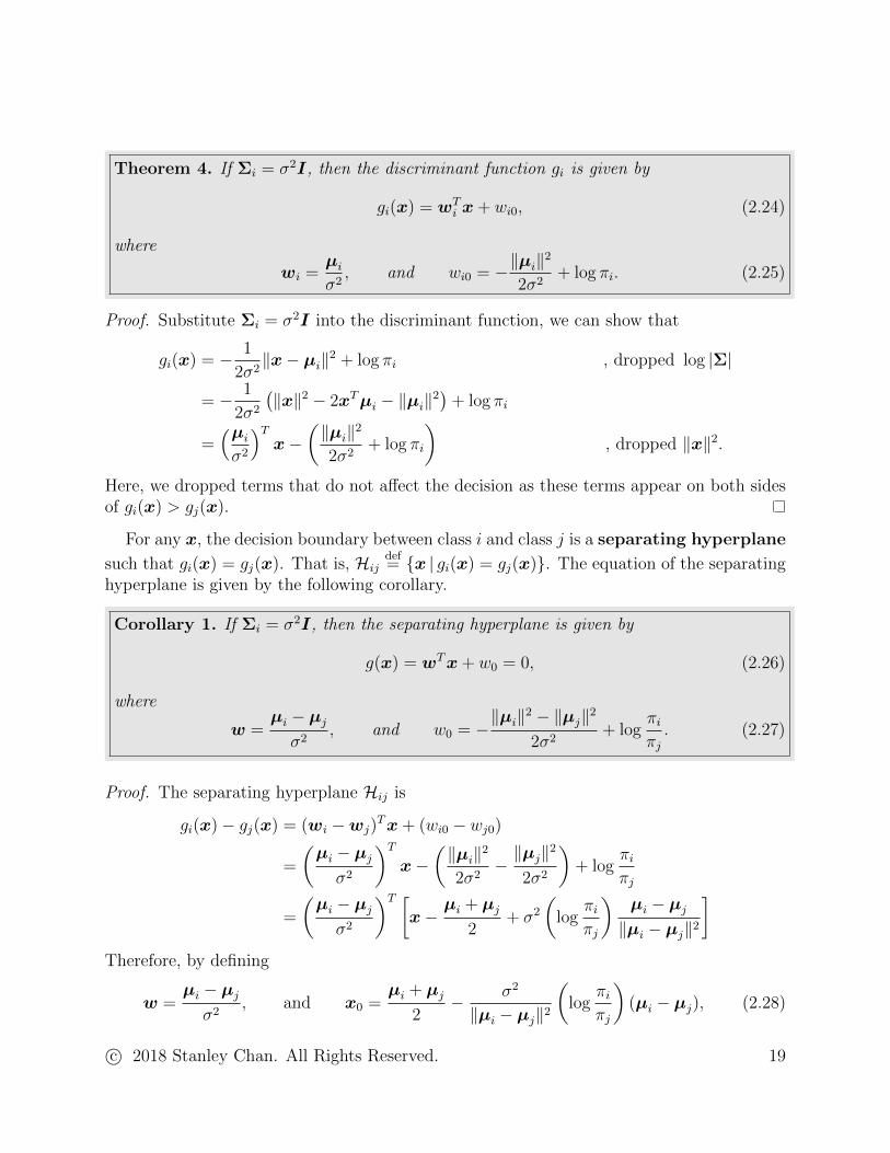
Theorem 4. If Σi = σ2I, then the discriminant function gi is given by

gi(x) = wTi x+ wi0, (2.24)

where

wi =µiσ2, and wi0 = −‖µi‖

2

2σ2+ log πi. (2.25)

Proof. Substitute Σi = σ2I into the discriminant function, we can show that

gi(x) = − 1

2σ2‖x− µi‖2 + log πi , dropped log |Σ|

= − 1

2σ2

(‖x‖2 − 2xTµi − ‖µi‖2

)+ log πi

=(µiσ2

)Tx−

(‖µi‖2

2σ2+ log πi

), dropped ‖x‖2.

Here, we dropped terms that do not affect the decision as these terms appear on both sidesof gi(x) > gj(x).

For any x, the decision boundary between class i and class j is a separating hyperplane

such that gi(x) = gj(x). That is, Hijdef= {x | gi(x) = gj(x)}. The equation of the separating

hyperplane is given by the following corollary.

Corollary 1. If Σi = σ2I, then the separating hyperplane is given by

g(x) = wTx+ w0 = 0, (2.26)

where

w =µi − µjσ2

, and w0 = −‖µi‖2 − ‖µj‖2

2σ2+ log

πiπj. (2.27)

Proof. The separating hyperplane Hij is

gi(x)− gj(x) = (wi −wj)Tx+ (wi0 − wj0)

=

(µi − µjσ2

)Tx−

(‖µi‖2

2σ2−‖µj‖2

2σ2

)+ log

πiπj

=

(µi − µjσ2

)T [x−

µi + µj2

+ σ2

(log

πiπj

)µi − µj‖µi − µj‖2

]Therefore, by defining

w =µi − µjσ2

, and x0 =µi + µj

2− σ2

‖µi − µj‖2

(log

πiπj

)(µi − µj), (2.28)


Figure 2.16: Geometry of a Bayes classifier when Σi = σ2I.

the separating hyperplane is equivalent to Hij ={x |wT (x− x0) = 0

}.

Geometrically, wij = µi − µj specifies the line passing through the centers of the twoclasses µi and µj. Thus, wT

ij(x−x0) = 0 gives the normal of the line. The point x0 specifiesthe location of the normal. The first term (µi + µj)/2 is the mid-point between µi andµj. When πi = πj so that log πi/πj = 0, the location is x0 = (µi + µj)/2 as there is nobias towards either class. As the ratio πi/πj changes, x0 will move along the line (µi −µj).The amount of the displacement is σ2

‖µi−µj‖2log πi/πj. Intuitively, the displacement scales

with the relative emphasis of πi and πj: If πi dominates, then log πi/πj is large and so x0 isshifted towards class 1. The displacement also scales with the reciprocal of ‖µi − µj‖2/σ2.If the two Gaussians are close, then for a positive log πi/πj the intercept x0 is shifted moretowards class 1. If log πi/πj becomes negative, then x0 is shifted towards class 2.

Exercise 2.2. Consider two 1D Gaussians with X|Y ∼ N (0, σ2) if Y = 0, and X|Y ∼N (µ, σ2) if Y = 1. Assume pY (i) = πi.

(i) Suppose we are given an observation X = x. Prove that the Bayesian decision ruleis given by

x ≶C0C1σ2

µlog

π0π1

+µ

2def= τ.

(ii) Let h(X) be the hypothesis function. Define the probability of error as

Pe = π1P[h(X) = 0|Y = 1] + π0P[h(X) = 1|Y = 0].

Express Pe in terms of the standard Normal CDF Φ(z) =∫ z−∞

1√2πe−t

2/2dt.

Hint: Note that h(X) = 0 iff X > τ , and h(X) = 1 iff X < τ .


Below is a MATLAB / Python code to generate a Bayesian decision rule for Σ = σ2I. Inthis demonstration, we use the population mean and covariance to compute the discriminantfunction. In practice, the population mean and covariance can be replaced by the empiricalmean and empirical covariance.

% MATLAB code to generate a decision boundary of the BDR

mu0 = [0; 0];

mu1 = [2; 1];

s = 0.5;

Sigma = (s^2)*[1 0; 0 1];

n = 1000;

w = (mu1-mu0)/s^2;

x0 = (mu1+mu0)/2;

y0 = mvnrnd(mu0,Sigma,[n,1]);

y1 = mvnrnd(mu1,Sigma,[n,1]);

To plot the decision boundary, we need to determine the two end points in the plot unless wehave some specialized plotting libraries. The two end points can be found sincewT (x−x0) =0. Rewriting this equation we have wTx = wTx0. Now, consider a two-dimensional case sothat d = 2. Then, wTx = wTx0 is equivalent to

w1x1 + w2x2 = wTx0.

If we set x1 to a constant, then we can determine x2 = (wTx0−w1x1)/w2. Vice versa, if weset x2 to a constant, we can determine x1 = (wTx0 − w2x2)/w1. In the plot below, we setx1 = 5 and x2 = 5 to locate the two extreme points.

figure;

scatter(y0(:,1),y0(:,2),’bo’); hold on;

scatter(y1(:,1),y1(:,2),’rx’);

plot([5, (w’*x0-w(2)*5)/w(1)]’, [(w’*x0-w(1)*5)/w(2), 5]’, ...

, ’k’, ’LineWidth’, 2);

axis([-2 3.5 -2 3.5]);

set(gcf, ’Position’, [100, 100, 500, 500]);

The plot of this example is shown in Figure 2.17. Because of the display, the aspectratio of the x-axis and the y-axis is not 1:1. Therefore, to properly visualize the decisionboundary, we can reset the aspect ratio. From there, we will be able to see the normal vectorw = (µ1 − µ0)/σ

2.


-2 -1.5 -1 -0.5 0 0.5 1 1.5 2 2.5 3 3.5

-2

-1.5

-1

-0.5

0

0.5

1

1.5

2

2.5

3

3.5

Figure 2.17: Bayesian decision rule using Σi = σ2I.

Case 2: Σi = Σ

In this case, we lift the assumption that Σi are scalar multiples of the identity matrix, butwe still assume that all Σi’s are the same. The discriminant function now becomes

gi(x) = −1

2(x− µi)TΣ−1(x− µi)−

1

2log |Σ|+ log πi. (2.29)

Theorem 5. If Σi = Σ, then the discriminant function gi is given by

gi(x) = wTi x+ wi0, (2.30)

where

wi = Σ−1µi, and wi0 = −1

2µTi Σ−1µi + log πi. (2.31)

Proof. The proof follows similarly with Case 1. We show that

gi(x) = −1

2(x− µi)TΣ−1(x− µi) + log πi

= −1

2

(xTΣ−1x− 2µTi Σ−1x+ µTi Σ−1µi

)+ log πi

= µTi Σ−1x− 1

2µTi Σ−1µi + log πi , dropped xTΣ−1x.

where terms irrelevant to the decision are dropped.


The geometry of the decision boundary can be analyzed by comparing gi(x)− gj(x):

gi(x)− gj(x) = (wi −wj)Tx+ (wi0 − wj0)

=[Σ−1(µi − µj)

]Tx− 1

2

(µTi Σ−1µi − µTj Σ−1µj

)+ log

πiπj.

This gives the following corollary about the separating hyperplaneHij = {x | wTx+w0 = 0}:

Corollary 2. If Σi = Σ, then the separating hyperplane is given by

g(x) = wTx+ w0 = 0, (2.32)

where

w = Σ−1(µi − µj), and w0 = −1

2

(µi + µj)

TΣ−1(µi − µj)

+ logπiπj. (2.33)

From this corollary, if we define

w = Σ−1(µi − µj), and x0 =µi + µj

2−

log πiπj

(µi − µj)TΣ−1(µi − µj)(µi − µj). (2.34)

then, we have gi(x) − gj(x) = wT (x − x0). Clearly, if Σ = σ2I, we will obtain the exactsame result as Case 1.

Figure 2.18: Geometry of a Bayes decision when the Gaussians have identical covariance matrices.

The inverse covariance matrix Σ−1 changes the decision boundary, as it applies a lineartransformation to the vector µi − µj. Such linear transformation is needed, because thecovariance matrix changes the shape of the two Gaussians. As a result, the decision boundaryshould adjust its orientation in order to match the underlying Gaussians.


Case 3: Arbitrary Σi

In the most general setting, the discriminant function takes the form of

gi(x) = −1


1


Theorem 6. If Σi is an arbitrary positive semi-definite matrix, then

gi(x) =1

2xTW ix+wT

i x+ wi0, (2.36)

where

W i = Σ−1i , wi = −Σ−1i µi, and wi0 =1

2µTi Σ−1i µi +

1

2log |Σi| − log πi.

Proof. The result follows from the fact that

gi(x) =1

2(x− µi)TΣ−1i (x− µi) +

1

2log |Σi| − log πi , changed to positive

=1

2xTΣ−1i x− µTi Σ−1i x+

1

2µTi Σ−1i µi +

1

2log |Σi| − log πi,

where we flipped the sign of gi as it does not affect the decision.

If we look at the decision boundary, we note that the decision boundary is given by

gi(x)− gj(x) =1

2xT (W i −W j)x+ (wi −wj)

Tx+ (wi0 − wj0). (2.37)

As a result, the geometry of the decision boundary is subject to the positive definiteness of

Wdef= W i −W j. If W is positive definite, then the decision boundary will be an ellipsoid.

If W has one positive eigenvalue and one negative eigenvalue, then the decision boundarywill be a hyperbolic paraboloid. Depending also on the magnitude of the eigenvalues, theellipse can be simplified to a sphere. Several examples are shown in Figure 2.19.

Exercise 2.3 Consider two inverse covariance matrices

W 1 =

[4 22 3

]and W 2 =

[5 11 2

]. (2.38)

(i) Compute the eigenvalues of W 1 and W 2 to show that both are positive semi-definite.

(ii) Show that W 1 −W 2 is symmetric. Does symmetry hold for all W 1 and W 2? Thatis, if W 1 and W 2 are both symmetric, is W 1 −W 2 also symmetric?

(iii) Show that W 1 −W 2 is neither positive semi-definite or negative semi-definite.


Figure 2.19: Geometry of a Bayes decision when the Gaussians are arbitrary. In this figure, Wdef= W i−W j ,

and w = wi−wj . The contour plots are taken from Wikipedia https://en.wikipedia.org/wiki/Quadric.

Maximum Likelihood

After discussing the geometry of the discriminant function, we should now ask a practicalproblem: Given a dataset D = {(xj, yj)}nj=1, how can we determine the model parameters{(µi,Σi)}ki=1? This parameter estimation problem is the training phase of the Bayesiandecision rule, for without such parameter estimation we will not be able to build the models.

For simplicity, let us assume thatD is partitioned into k non-overlapping subsetsD1, . . . ,Dk.Each Di = {(x(i)

j , y(i)j )}nj=1 is the training set for class i, and this training set will give us the

parameter (µi,Σi). To reduce notation burden we shall drop the subscript i unless confusionarises for different classes.

Given D, our goal is to estimate the model parameter θ. If we assume that D is drawnfrom a distribution, and θ is its model parameter, then the most straight-forward approachis to find a θ that maximizes the probability of generating D:

θ̂ = argmaxθ

p(D ; θ)

= argmaxθ

n∏j=1

p(xj;θ). (2.39)


Here, the distribution p(D ; θ) means the joint distribution of all samples in D, and thisjoint distribution is specified by a parameter θ. The second equality in the above equationis based on an important assumption that all the m samples in D are independent.

Let us look at one example. Suppose that we assume D is a multi-dimensional Gaussianwith known Σ. Then the parameter is the unknown mean: θ = µ. The optimization istherefore

µ̂ = argmaxµ

n∏j=1

1√(2π)d|Σ|

exp

{−1

2(xj − µ)TΣ−1(xj − µ)

}

= argmaxµ

(1√

(2π)d|Σ|

)n

exp

{−1

2

n∑j=1

(xj − µ)TΣ−1(xj − µ)

}. (2.40)

Now we can apply a useful trick (again!): Since log is monotonically increasing, we can applylog to the right hand side and it will not affect the maximizer. Further, if we take − log wecan flip the maximum to minimum. Therefore, we can show that

µ̂ = argminµ

1

2

n∑j=1

(xj − µ)TΣ−1(xj − µ). (2.41)

Taking the derivative and setting to zero, we can show that

∇µ

{1

2

n∑j=1

(xj − µ)TΣ−1(xj − µ)

}=

n∑j=1

Σ−1(xj − µ) = 0.

Moving the terms around, and noting that∑n

j=1µ = nµ, the solution is

µ̂ =1

n

n∑j=1

xj. (2.42)

We call this solution the maximum-likelihood estimate of the multi-dimensional Gaussian.The implication of this result is that for a given dataset D, the maximum-likelihood estimateof mean of a multi-dimensional Gaussian is simply the empirical average of the dataset.

Theorem 7 (Maximum-Likelihood Estimate for Mean). Assume D is generated from amulti-dimensional Gaussian with an unknown mean µ and a fixed covariance Σ. Themaximum-likelihood estimate of µ is

µ̂ = argmaxµ

n∏j=1

1√(2π)d|Σ|

exp

{−1

2(xj − µ)TΣ−1(xj − µ)

}

=1

n

n∑j=1

xj. (2.43)


Figure 2.20: Pictorial illustration of maximum likelihood estimation.

Let us take a look at the geometric interpretation. Consider a 1D problem so that d = 1.By switching the mean, we will construct a family of Gaussians N (µ, σ2), where the runningindex is the mean µ. When there is only one observation (n = 1) so that we only have x1, theMLE estimate of the mean is exactly the sample µ = x1. This is equivalent to ask: Amongthe different Gaussians, which one can maximize the probability of getting the sample x1.Clearly, this happens when x1 is located at the center of the Gaussian, and so the bestGaussian is N (x1, σ

2).Now, if we increase the number of observations to n = 2 so that we have x1 and x2, the

MLE estimate of the mean is µ = (x1 + x2)/2. This is equivalent to asking: Given x1 andx2, which Gaussian is the most likely one that can simultaneously give x1 and x2? And fromour calculation, we know that the Gaussian should be centered at the mid point of x1 andx2, and so that best Gaussian is N ((x1 + x2)/2, σ

2). As n increases, we eventually haveµ = 1

n

∑nj=1 xj.

Exercise 2.3. The theorem above requires a known covariance Σ. If we assume that boththe mean µ and the covariance Σ are unknown, then the maximum-likelihood estimate of(µ,Σ) becomes

µ̂ =1

n

n∑j=1

xj, and Σ̂ =1

n

n∑j=1

(xj − µ)(xj − µ)T , (2.44)

which are called the sample mean, and the sample covariance, respectively.

(i) Prove that E[Σ̂] 6= Σ, where the expectation is taken with respect to xj. This showsthe sample covariance is biased.

(ii) Prove that if Σ̂ = 1n−1

∑nj=1(xj − µ)(xj − µ)T , then we have E[Σ̂] = Σ.


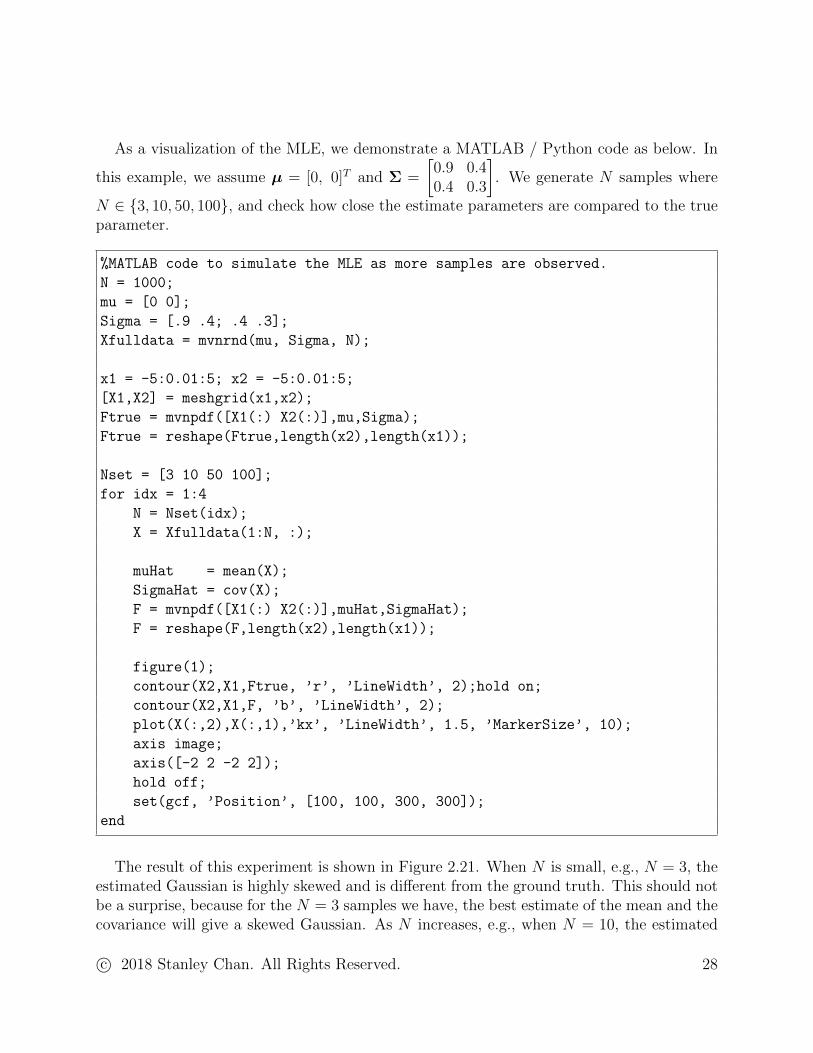
As a visualization of the MLE, we demonstrate a MATLAB / Python code as below. In

this example, we assume µ = [0, 0]T and Σ =

[0.9 0.40.4 0.3

]. We generate N samples where

N ∈ {3, 10, 50, 100}, and check how close the estimate parameters are compared to the trueparameter.

%MATLAB code to simulate the MLE as more samples are observed.

N = 1000;

mu = [0 0];

Sigma = [.9 .4; .4 .3];

Xfulldata = mvnrnd(mu, Sigma, N);

x1 = -5:0.01:5; x2 = -5:0.01:5;

[X1,X2] = meshgrid(x1,x2);

Ftrue = mvnpdf([X1(:) X2(:)],mu,Sigma);

Ftrue = reshape(Ftrue,length(x2),length(x1));

Nset = [3 10 50 100];

for idx = 1:4

N = Nset(idx);

X = Xfulldata(1:N, :);

muHat = mean(X);

SigmaHat = cov(X);

F = mvnpdf([X1(:) X2(:)],muHat,SigmaHat);

F = reshape(F,length(x2),length(x1));

figure(1);

contour(X2,X1,Ftrue, ’r’, ’LineWidth’, 2);hold on;

contour(X2,X1,F, ’b’, ’LineWidth’, 2);

plot(X(:,2),X(:,1),’kx’, ’LineWidth’, 1.5, ’MarkerSize’, 10);

axis image;

axis([-2 2 -2 2]);

hold off;

set(gcf, ’Position’, [100, 100, 300, 300]);

end

The result of this experiment is shown in Figure 2.21. When N is small, e.g., N = 3, theestimated Gaussian is highly skewed and is different from the ground truth. This should notbe a surprise, because for the N = 3 samples we have, the best estimate of the mean and thecovariance will give a skewed Gaussian. As N increases, e.g., when N = 10, the estimated


Gaussian becomes more similar to the ground truth; And ultimately when we have enoughsamples, e.g., N = 100, the estimated Gaussian starts to overlap with the ground truthGaussian.

Figure 2.21: Estimating the Gaussian parameters using MLE as number of samples increases. From left toright: N = 3, N = 10, N = 50, and N = 100. As more samples become available, the estimated Gaussianbecomes more similar to the ground truth Gaussian.

Maximum-a-Posteriori

While maximum-likelihood estimate is simple and straight-forward, a practical question weask is how to improve the ML estimates when m is small? However, when m is small, thereis really not much we can do because the dataset D is small. In this case, we need to makesome prior assumptions about θ. In Bayesian terminology, we assume a θ is sampled froma prior distribution pΘ(θ), and write the posterior distribution as

p(θ | D) ∝ p(D |θ)p(θ). (2.45)

Let us look at the terms on the right hand side. What is the difference between p(D ; θ) inmaximum likelihood and p(D |θ) in this expression? The probability in maximum-likelihoodp(D ; θ) assumes that θ is a deterministic parameter. There is nothing random about θ.The probability we have here p(D |θ) assumes that θ is a realization of a random variableΘ. Thus, there is a distribution of θ, which is pΘ(θ) or simply p(θ). Because of the priordistribution, we can talk about the posterior distribution of θ given D. This posteriordistribution is undefined for maximum likelihood, because there is no distribution for θ.

If we take this route, then a natural solution for the estimation problem is to maximizethe posterior distribution:

θ̂ = argmaxθ

p(D |θ)p(θ) = argmaxθ

n∏j=1

p(xj |θ)p(θ). (2.46)

The solution to this problem is called the maximum-a-posteriori (MAP) estimation.


Let us look at a 1D example. Suppose that the observations {xj}nj=1 are generated froma Gaussian N (µ, σ2) where σ is a known and fixed constant. Our goal is to estimate theunknown mean θ. We assume that θ is generated from a prior distribution p(θ) which isanother Gaussian:

p(x|µ) =1√

2πσ2exp

{−(x− µ)2

2σ2

}, and p(µ) =

1√2π

exp

{−µ

2

2

}.

Now, given the observations {xj}nj=1, the MAP estimate is determined by solving the problem

µ̂ = argmaxµ

n∏j=1

p(xj|µ)p(µ)

= argmaxµ

(1√

2πσ2

)Nexp

{−

n∑j=1

(xj − µ)2

2σ2

}· 1√

2πexp

{−µ

2

2

}

= argmaxµ

−

(n∑j=1

(xj − µ)2

2σ2+µ2

2

)

=

∑nj=1 xj

n+ σ2.

The above equation shows that the effect of the prior p(µ) lies in the denominator of thefractions. For small n, the factor σ2 has more influence. This can be understood as when wehave few observations, we should rely more on the prior. However, as n grows, the influenceof the prior reduces and we put more emphasis on the observations.

Pictorially, the presence of a prior changes the “best” Gaussian from a purely observation-based result to a experience plus observation result. An illustration is shown in Figure 2.22.

Figure 2.22: The green curve is the prior distribution p(µ). When N = 1, the best Gaussian is shifted fromx1 according to the prior. Similarly for n = 2, the best Gaussian is shifted according to the prior and theobservations x1 + x2.

Now, let us generalize to a high-dimensional Gaussian. Consider xj |µ ∼ N (µ,Σ0), andµ ∼ N (µθ,Σθ). Assume that Σ0 is fixed and known. The interpretation of this setting isthat the sample xj has a conditional distribution N (µ,Σ0). The conditional mean µ has


its own distribution N (µθ,Σθ). In this case, the posterior distribution can be written as

µ̂ = argmaxµ

p(µ | D) = argmaxµ

n∏j=1

p(xj |µ)p(µ)

= argmaxµ

(n∏j=1

exp

{−1

2(xj − µ)TΣ−10 (xj − µ)

})· exp

{−1

2(µ− µθ)TΣ−1θ (µ− µθ)

}

= argmaxµ

C exp

{−1

2

(µT (mΣ−10 + Σ−1θ )µ− 2µT

(Σ−10

n∑j=1

xj + Σ−1θ µθ

))}

= argmaxµ

C ′ exp

{−1

2(µ− µ̃)T Σ̃

−1(µ− µ̃)

}= µ̃,

where with some (slightly tedious) algebra we can show that

µ̃ = Σθ

(Σθ +

1

nΣ0

)−1(1

n

n∑j=1

xj

)+

1

nΣ0

(Σθ +

1

nΣ0

)−1µθ,

Σ̃ = Σθ

(Σθ +

1

nΣ0

)−11

nΣ0. (2.47)

Theorem 8 (Maximum-a-Posteriori Estimate for Mean). Assume D is generated from amulti-dimensional Gaussian with xj |µ ∼ N (µ,Σ0), and µ ∼ N (µθ,Σθ). maximum-a-posteriori estimate of µ is

µ̂ = argmaxµ

n∏j=1

p(xj |µ)p(µ)

= Σθ

(Σθ +

1

nΣ0

)−1(1

n

n∑j=1

xj

)+

1

nΣ0

(Σθ +

1

nΣ0

)−1µθ. (2.48)

Can we say something about the Theorem? If we let m→∞, we can show that

limn→∞

{Σθ

(Σθ +

1

nΣ0

)−1(1

n

n∑j=1

xj

)+

1

nΣ0

(Σθ +

1

nΣ0

)−1µθ

}= lim

n→∞

1

n

n∑j=1

xj,

which means that the MAP estimate is asymptotically equivalent to the ML estimate.Putting in simple words, the result implies that when m is large, MAP estimates and MLestimates will return the same result. If we want to be specific about this limit, we can applyLaw of Large Number to show that lim

n→∞1n

∑nj=1 xj

a.s.→ E[X].


If n is small, Equation (2.48) suggests that the estimate mean is a linear combination ofthe ML estimate 1

n

∑nj=1 xj and the prior mean µθ. Therefore, MAP offers side information

about the estimation using the prior. The side information is useful when n is small, butwill be override by the ML estimate when n grows.

Exercise 2.4. Consider a 1D problem where the Gaussian are xj |µ ∼ N (µ, σ0), andµ ∼ N (µθ, σθ).

(i) Show that the MAP estimate of the mean is

µ̂ =

(nσ2

θ

nσ2θ + σ2

0

)(1

n

n∑j=1

xj

)+

σ20

nσ2θ + σ2

0

µθ. (2.49)

(ii) Comment on the situations when n→∞, when σ0 → 0, or when σθ → 0. What arethe physical interpretations?

2.3 Linear Regression

The Bayes decision rule we see in the previous section is a generative method, as we needto assume a generative model that generates the data. In this section we study anothermethod called the discriminative method which does not assume any generative model.Generative methods and discriminative methods will both lead to a discriminant functiongi(x). If we assume a linear discriminant function gθ(x) = wTx + w0, then the ultimategoal of both methods is to determine the model parameters θ = (w, w0). In this section wediscuss a discriminative method called linear regression.

To make things simple, let us focus on a binary classification problem with a discriminantfunction gθ(x) = wTx + w0. We assume that we have a set of training data (xj, yj)

nj=1,

where xj is the feature vector and yj ∈ {−1,+1} is the corresponding label. The overalltraining loss of the dataset is defined as

J(θ) =1

n

n∑j=1

(gθ(xj)− yj)2 =1

n

n∑j=1

(wTxj + w0 − yj)2

=

∥∥∥∥∥∥∥x

T1 1...

...xTn 1

[ww0

]−

y1...yn

∥∥∥∥∥∥∥2

= ‖Xθ − y‖2, (2.50)

where we define

X =

xT1 1...

...xTn 1

, θ =

[ww0

]and y =

y1...yn

.c© 2018 Stanley Chan. All Rights Reserved. 32

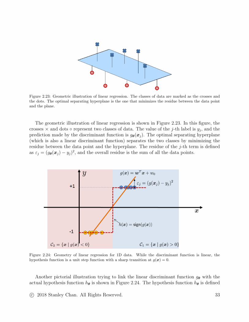
Figure 2.23: Geometric illustration of linear regression. The classes of data are marked as the crosses andthe dots. The optimal separating hyperplane is the one that minimizes the residue between the data pointand the plane.

The geometric illustration of linear regression is shown in Figure 2.23. In this figure, thecrosses × and dots ◦ represent two classes of data. The value of the j-th label is yj, and theprediction made by the discriminant function is gθ(xj). The optimal separating hyperplane(which is also a linear discriminant function) separates the two classes by minimizing theresidue between the data point and the hyperplane. The residue of the j-th term is definedas εj = (gθ(xj)− yj)2, and the overall residue is the sum of all the data points.

Figure 2.24: Geometry of linear regression for 1D data. While the discriminant function is linear, thehypothesis function is a unit step function with a sharp transition at g(x) = 0.

Another pictorial illustration trying to link the linear discriminant function gθ with theactual hypothesis function hθ is shown in Figure 2.24. The hypothesis function hθ is defined


as

hθ(x) = sign(gθ(x)) =

{+1, if gθ(x) = wTx+ w0 > 0,

−1, if gθ(x) = wTx+ w0 ≤ 0.(2.51)

Figure 2.24 shows two classes of data with labels y = +1 and y = −1. By assuming alinear model, we seek a straight line wTx + w0 that best describes these data points byminimizing the sum of the individual error εj = (gθ(xj)− yj)2. Once the model parametersθ are determined, we form a decision rule by checking whether gθ(x) > 0 for any testingdata x. This gives us the two decision regions C1 and C2.

Solution of Linear Regression

To obtain the optimal parameter θ, we minimize the loss function:

θ∗ = argminθ

J(θ) = ‖Xθ − y‖2.

So how do we solve this optimization problem? If we take the gradient and set to zero, wewill have

∇θJ(θ) = ∇θ‖Xθ − y‖2

= ∇θ{θTXTXθ − 2yTXθ + ‖y‖2

}= 2XTXθ − 2XTy

= 0.

Rearranging terms we can show the so called normal equation: XTXθ = XTy, of whichthe solution is given by

θ∗ = (XTX)−1XTy. (2.52)

We can summarize these findings in the following Theorem.

Theorem 9 (Linear Regression Solution). The loss function of a linear regression modelis given by

J(θ) = ‖Xθ − y‖2, (2.53)

of which the minimizer isθ∗ = (XTX)−1XTy. (2.54)

For some large-scale datasets with many variables, we may want to use iterative algorithmssuch as gradient descent to compute the solution. In this case, the gradient descent algorithmis given by the iteration

θ(k+1) = θ(k) − η∇θJ(θ(k))

= θ(k) − η(2XTXθ(k) − 2XTy).


for some step sizes η. A pictorial illustration of the gradient descent step is shown inFigure 2.25. As we update θ(k), we construct a sequence θ(1),θ(2), . . .. Each θ(k) is theparameter of a linear discriminant function. When θ(k) is closer to the minimum value ofthe loss function J(θ), the corresponding discriminant function will be able to separate moredata points into two classes.

Figure 2.25: Gradient descent of linear regression. [Right] Gradient descent algorithm seeks a sequence θ(k)

by searching along the steepest descent direction. The sequence θ(k) moves towards the minimum of J(θ).

[Left] As θ(k) moves closer to the minimum point, the discriminant function improves its ability to separatethe two classes.

Does the gradient descent algorithm converge, and if it does, is the solution unique? Inthe following exercise we will show that J is convex for any X. Therefore, gradient descentwith appropriate step size is guaranteed to find the optimal solution, and the objective valueJ(θ∗) is unique. However, the solution θ∗ is unique only when J is strictly convex.

Exercise 3.1. Consider the loss function J(θ) = ‖Xθ − y‖2.

(i) Prove that J is always convex in θ, regardless of the choice of X. Hint: We caneither prove that J(λθ1 + (1− λ)θ2) ≤ λJ(θ1) + (1− λ)J(θ2), or show that ∇2J(θ)is positive semi-definite.

(ii) Prove that the optimal solution θ∗ is unique if and only if J is strictly convex. Hint:Show by contradiction that if θ∗1 and θ∗2 are both optimal with θ∗1 6= θ∗2, then anyconvex combination will also be optimal.

Regularization

What should we do if XTX is not invertible? One simple but practical approach is toconsider a regularized linear regression:

J(θ) = ‖Xθ − y‖2 + λρ(θ), (2.55)


where ρ : Rd+1 → Rd+1 is the regularization function. For example, if ρ(θ) = ‖θ‖2, then

J(θ) = ‖Xθ − y‖2 + λ‖θ‖2. (2.56)

In signal processing, this minimization is called the Tikhonov regularized least squares;In statistics, this is called the ridge regression. In either case, the minimizer of J satisfies

∇θJ(θ) = ∇θ‖Xθ − y‖2 + λ‖θ‖2

= 2XT (Xθ − y) + 2θ = 0,

which gives us

θ∗ = (XTX + λI)−1XTy.

It is not difficult to see that the new matrix XTX + λI is always invertible. If we do aneigen-decomposition of XTX by writing XTX = U |S|2UT , then

XTX + λI = U |S|2UT + λUUT = U(|S|2 + λI)UT .

Therefore, the j-th eigenvalue of XTX + λI is s2j + λ > 0. However, in getting bettermatrices to invert, the price we pay is that we no longer allow large entries in θ, for largeentries in θ will be heavily penalized by the regularization λ‖θ‖2. In the extreme if λ→∞,then the optimal solution will become θ∗ = 0.

Exercise 3.2. Consider the loss function

J(θ) = ‖Xθ − y‖2 + λρ(θ).

(i) Prove that if ρ is convex, then J is convex.

(ii) Let ρ(θ) = ‖Bθ‖2 for some matrix B ∈ R(d+1)×(d+1). Find the optimal θ∗.

In modern statistical learning, powerful regularization functions ρ are typically non-differentiable, e.g., ρ(θ) = ‖θ‖1. The corresponding optimization

J(θ) = ‖Xθ − y‖2 + λ‖θ‖1 (2.57)

is called the LASSO (stands for Least Absolute Shrinkage and Selection Operator). LASSOhas many nice properties such as: (i) It promotes sparsity of θ, i.e., forcing many entries ofθ to zero so that we can compress the set of active features; (ii) It is the tightest convexrelaxation of the NP-hard ‖θ‖0; (iii) Although ‖θ‖1 is non-differentiable (at θ = 0), thereexits polynomial time convex solvers to solve the problem, e.g., interior point methods, oralternating direction method of multipliers.


Linear Regression beyond Classification

Linear regression can be used for applications beyond classification. As a demonstrationof linear regression and illustrating how `1 regularization is used, we study a data fittingproblem. Given a dataset consisting of multiple attributes, we can construct a data matrix

X =

| | |x1 x2 . . . xd| | |

, (2.58)

where each column xj ∈ Rn is a feature vector. These feature vectors can be considered asthe contributing factors of observing the vector y ∈ Rn via a set of regression coefficientsθ ∈ Rd. This means

y ≈d∑j=1

θjxj = Xθ. (2.59)

The optimal regression coefficient can then be found as

θ̂ = argminθ

‖Xθ − y‖2.

To see a concrete example, we use the crime rate data obtained from https://web.

stanford.edu/~hastie/StatLearnSparsity/data.html. A snapshot of the data is shownin Figure 2.26. In this dataset, the vector y is the crime rate, which is the last column ofFigure 2.26. The feature vectors are funding, hs, not-hs, college, college4.

Figure 2.26: Crime rate data. Extracted from Hastie and Tibshirani’s Statistical Learning with Sparsity.

The following MATLAB / Python code is used to extract the data.

data = load(’data_crime.txt’);

y = data(:,1); % The observed crime rate

A = data(:,3:end); % Feature vectors

[m,n] = size(A);


Once we have extracted the data from the dataset, we consider two optimizations

θ̂1(λ) = argminθ

J1(θ)def= ‖Xθ − y‖22 + λ‖θ‖1,

θ̂2(λ) = argminθ

J2(θ)def= ‖Xθ − y‖22 + λ‖θ‖22.

As we have discussed, the first optimization is the `1 regularized least squares which isalso called the LASSO problem. The second optimization is the standard `2 regularizedleast squares. We use regularization instead of solving the bare linear regression becausethe raw data does not guarantee an invertible matrix XTX. Now, in this experiment, wewould like to visualize the linear regression coefficients θ̂1(λ) and θ̂2(λ) as the regularizationparameter λ changes. To solve the optimization, we use CVX with the MATLAB / Pythonimplementation shown below.

% MATLAB code to solve L1 and L2 minimization, and visualize the result

lambdaset = logspace(-1,8,50);

x_store = zeros(5,length(lambdaset));

for i=1:length(lambdaset)

lambda = lambdaset(i);

cvx_begin

variable x(n)

minimize( sum_square( A*x - y ) + lambda * norm(x , 1) )

% minimize( sum_square( A*x - y ) + lambda * sum_square(x) )

cvx_end

x_store(:,i) = x(:);

end

semilogx(lambdaset, x_store, ’LineWidth’, 2);

legend(’funding’,’high’, ’no high’, ’college’, ’graduate’, ’Location’,’NW’);

xlabel(’lambda’);

ylabel(’feature attribute’);

The result in Figure 2.27 shows some interesting differences between the two linear regres-sion models. For the `2 estimate θ2(λ), the trajectory of the regression coefficients is smoothas λ changes. This is attributed to the fact that the `2 optimization cost J2(θ) is continuouslydifferentiable in θ, and so the solution trajectory is smooth. In contrast, the `1 estimate θ1(λ)has a more disruptive trajectory. As λ reduces, the feature percentage of high-school isfirst activated. A possible implication is that if we are to limit ourselves to one most salientfeature, then the percentage of high-school is the feature we should select. As such, thetrajectory of the regression coefficient shows an ordered list of features that are contributingto the observation. As λ → 0, both θ1(λ) and θ2(λ) reach the same solution, as the costfunctions become identical.


10−2

100

102

104

106

108

−2

0

2

4

6

8

10

12

14

lambda

featu

re a

ttribu

te

funding

% high

% no high

% college

% graduate

10−2

100

102

104

106

108

−2

0

2

4

6

8

10

12

14

lambda

featu

re a

ttribu

te

funding

% high

% no high

% college

% graduate

Figure 2.27: Crime rate data. Extracted from Hastie and Tibshirani’s Statistical Learning with Sparsity.

Connection with Bayesian Decision Rule

Unlike the Bayes decision rule, linear regression does not assume any probabilistic modelingof the data. However, if we insist of putting a probabilistic model, then we can argue thatthe loss function J(θ) converges almost surely to its expectation (via Strong / Weak Law ofLarge Number):

1

n

n∑j=1

(g(xj)− yj)2p−→ EX,Y [g(X)− Y )2]. (2.60)

Here, we have a small abuse of notation to denote X as a random variable in Rd thatgenerates the samples xj. By minimizing J(θ), we are essentially minimizing the expectation:

θ∗ = argminw,w0

1

n

n∑j=1

(g(xj)− yj)2

= argminw,w0

EX,Y

[(wTX + w0 − Y )2

]. (2.61)

Taking the derivatives with respect to (w, w0) yields

d

dwEX,Y

[(wTX + w0 − Y )2

]= 2

(E[XXT ]w + E[X]w0 − E[XY ]

), (2.62)

d

dw0

EX,Y

[(wTX + w0 − Y )2

]= 2

(E[X]Tw + w0 − E[Y ]

), (2.63)

where the expectations are taken over the joint distribution pX,Y (x, y). Bayes Theoremallows us to decompose pX,Y (x, y) = pX|Y (x|i)pY (i). If we assume that the conditionaldistribution pX|Y (x|i) is Gaussian with identical covariance:

pX|Y (x|i) =1√

2π|Σ|exp

{−1

2(x− µi)TΣ−1(x− µi)

}, i ∈ {−1,+1} (2.64)


and the prior is equal pY (i) = 12, then we have E[Y ] = 0. Moreover, we can show that the

expectation of X and E[XY ] are

E[X] =∑

i∈{−1,+1}

E[X|Y = i]pY (i) =1

2(µ1 + µ−1)

E[XY ] =∑

i∈{−1,+1}

E[XY |Y = i]pY (i) =1

2(µ1 − µ−1).

The covariance can be shown as

E[XXT ]− E[X]E[X]T = E[(X − E[X])(X − E[X])T ]

=∑

i∈{−1,+1}

E[(X − E[X])(X − E[X])T |Y = i

]pY (i)

=1

2Σ +

1

2Σ = Σ.

Consequently, if we multiply E[X] to Equation (2.63) and subtract from Equation (2.62),we will obtain

(E[XXT ]− E[X]E[X]T )w = E[XY ]− E[X]E[Y ], (2.65)

which gives

Σw =1

2(µ1 − µ−1) =⇒ w =

1

2Σ−1(µ1 − µ−1). (2.66)

Substituting into Equation (2.63), we have

w0 = −E[X]Tw = −1

2(µ1 + µ−1) ·

1

2Σ−1(µ1 − µ−1)

= −1

4(µ1 + µ−1)Σ

−1(µ1 − µ−1). (2.67)

Hence, the optimal (w∗, w∗0) satisfies

w∗ =1

2Σ−1(µ1 − µ−1) = Σ̃

−1(µ1 − µ−1)

w∗0 = −1

4(µ1 + µ−1)Σ

−1(µ1 − µ−1) = −1

2(µ1 + µ−1)Σ̃

−1(µ1 − µ−1), (2.68)

if we define Σ̃def= Σ/2.

In summary, the separating hyperplane returned by linear regression coincides with theseparating hyperplane returned by Bayes (Case 1 and Case 2) if πi = πj, i.e., the priors areidentical. (Case 3 does not work here because Case 3 is intrinsically quadratic, which cannotbe Bayesped to a linear classifier.) The result is summarized as below.


Figure 2.28: Linear regression coincides with the Gaussian Bayes when the covariances are identical, andthe priors are the same.

Theorem 10 (Conditions for Linear Regression = Bayes). Suppose that all the followingtwo conditions are satisfied:(i) the likelihood pX|Y (x|i) is Gaussian satisfying Equation (2.64),(ii) the prior is uniform: pY (i) = 1

2for i ∈ {+1,−1},

(iii) the number of training samples goes to infinity, i.e., the empirical average in in Equa-tion (2.60) converges to the expectation.Then, the linear regression model parameter (w, w0) is given by

w = Σ̃−1

(µ1 − µ−1), w0 = −1

2(µ1 + µ−1)Σ̃

−1(µ1 − µ−1), (2.69)

where Σ̃def= Σ/2, and Σ is the covariance of the Gaussian.

As a special case, if Σ̃ = σ2

2I, then (w, w0) is given by

w =µ1 − µ−1

2σ2, w0 = −

‖µ1‖2 − ‖µ−1‖2

2σ2, (2.70)

which is exactly the same as Case 1 with πi = πj.Figure 2.28 illustrates the situation in 1D, where we pose a Gaussian distribution to each

class. By assuming that the covariance matrices of the two Gaussians are equal, and byassuming that the priors are the same, we force the decision boundary wTx+w0 to be right


at the middle of the two classes. This could be sub-optimal, because by assuming π+1 = π−1we implicitly assume that the two classes have equal influence. We are also losing controlover cases where Σ+1 6= Σ−1, which could again be sub-optimal.

2.4 Logistic Regression

Putting aside the equal covariance assumption, there are two additional drawbacks of linearregression. First, the discriminant function g(x) is a straight line through the two clusters.Since the line passes through the center of each cluster, data points sitting farther from thecenter will have a large fitting error. Thus, it would be better to replace the linear modelwith a function that is closer to sign(·). The second drawback is the smooth transition atthe decision boundary. Again, if we can use a function that is closer to sign(·), we can makethe transition sharp.

Logistic regression is an alternative to the linear regression. Instead of constructing aclassifier through a two-step approach, i.e., first define a discriminant function g(x) = wTx+w0 and then define a hypothesis function h(x) = sign(g(x)), logistic regression directlyapproximates the hypothesis function h(x) using a logistic function:

h(x) =1

1 + e−g(x)=

1

1 + e−(wTx+w0)=

e(wTx+w0)

1 + e(wTx+w0). (2.71)

How does a logistic function look like? If we ignore the linear component wTx + w0 fora while by just looking at a 1D function

h(x) =1

1 + e−a(x−x0), for some a and x0, (2.72)

we note that

h(x)→ 1, as x→∞,h(x)→ 0, as x→ −∞, (2.73)

and there is a cutoff at x = x0, which gives h(x0) = 1/2. The sharpness of the transientis determined by the magnitude of the constant a: Larger a gives a sharper transient, andsmaller a gives s slower transient. The location of the cutoff is determined by the offset x0.If we make x0 larger, then the cut is shifted towards the right; otherwise it is shifted towardsthe left. A pictorial illustration is shown in Figure 2.29.

For high-dimensional vectors, the geometry of the hypothesis function is determined by thelinear component wTx+ w0. The cutoff happens at a point x0 ∈ Rd such that wTx0 = w0.The orientation and sharpness of the cutoff transient is determined by the plane wTx. Sincew is often bounded, the hypothesis function h(x)→ 1 when ‖x‖ → ∞, and h(x)→ 0 when‖x‖ → −∞. Essentially, this separates the space into two half-spaces, one taking the value1 and the other taking the value 0.


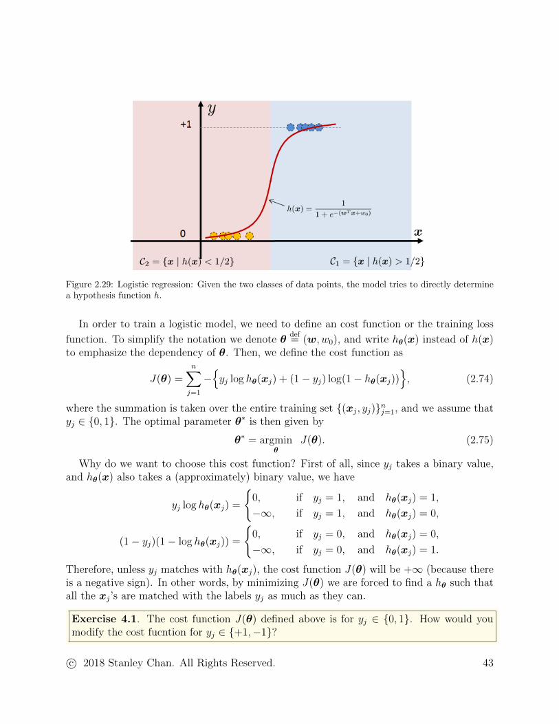
Figure 2.29: Logistic regression: Given the two classes of data points, the model tries to directly determinea hypothesis function h.

In order to train a logistic model, we need to define an cost function or the training loss

function. To simplify the notation we denote θdef= (w, w0), and write hθ(x) instead of h(x)

to emphasize the dependency of θ. Then, we define the cost function as

J(θ) =n∑j=1

−{yj log hθ(xj) + (1− yj) log(1− hθ(xj))

}, (2.74)

where the summation is taken over the entire training set {(xj, yj)}nj=1, and we assume thatyj ∈ {0, 1}. The optimal parameter θ∗ is then given by

θ∗ = argminθ

J(θ). (2.75)

Why do we want to choose this cost function? First of all, since yj takes a binary value,and hθ(x) also takes a (approximately) binary value, we have

yj log hθ(xj) =

{0, if yj = 1, and hθ(xj) = 1,

−∞, if yj = 1, and hθ(xj) = 0,

(1− yj)(1− log hθ(xj)) =

{0, if yj = 0, and hθ(xj) = 0,

−∞, if yj = 0, and hθ(xj) = 1.

Therefore, unless yj matches with hθ(xj), the cost function J(θ) will be +∞ (because thereis a negative sign). In other words, by minimizing J(θ) we are forced to find a hθ such thatall the xj’s are matched with the labels yj as much as they can.

Exercise 4.1. The cost function J(θ) defined above is for yj ∈ {0, 1}. How would youmodify the cost fucntion for yj ∈ {+1,−1}?


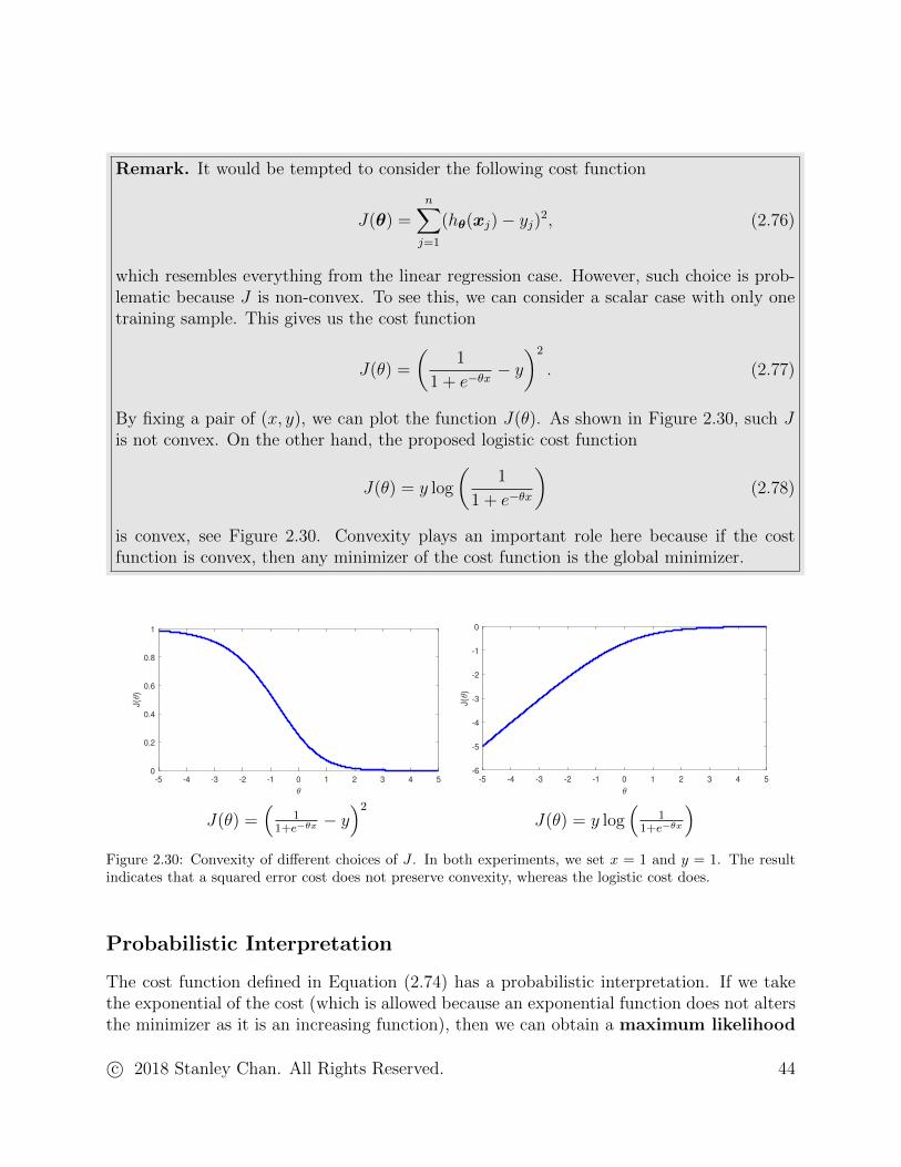
Remark. It would be tempted to consider the following cost function

J(θ) =n∑j=1

(hθ(xj)− yj)2, (2.76)

which resembles everything from the linear regression case. However, such choice is prob-lematic because J is non-convex. To see this, we can consider a scalar case with only onetraining sample. This gives us the cost function

J(θ) =

(1

1 + e−θx− y)2

. (2.77)

By fixing a pair of (x, y), we can plot the function J(θ). As shown in Figure 2.30, such Jis not convex. On the other hand, the proposed logistic cost function

J(θ) = y log

(1

1 + e−θx

)(2.78)

is convex, see Figure 2.30. Convexity plays an important role here because if the costfunction is convex, then any minimizer of the cost function is the global minimizer.

-5 -4 -3 -2 -1 0 1 2 3 4 50

0.2

0.4

0.6

0.8

1

J(

)

-5 -4 -3 -2 -1 0 1 2 3 4 5-6

-5

-4

-3

-2

-1

0

J(

)

J(θ) =(

11+e−θx

− y)2

J(θ) = y log(

11+e−θx

)Figure 2.30: Convexity of different choices of J . In both experiments, we set x = 1 and y = 1. The resultindicates that a squared error cost does not preserve convexity, whereas the logistic cost does.

Probabilistic Interpretation

The cost function defined in Equation (2.74) has a probabilistic interpretation. If we takethe exponential of the cost (which is allowed because an exponential function does not altersthe minimizer as it is an increasing function), then we can obtain a maximum likelihood


estimation of a Bernoulli distribution:

argminθ

J(θ) = argminθ

n∑j=1


}= argmin

θ− log

(n∏j=1

hθ(xj)yj(1− hθ(xj))1−yj

)

= argmaxθ

n∏j=1

{hθ(xj)

yj(1− hθ(xj))1−yj}. (2.79)

Putting in an other way, we can interpret hθ(xj) as the posterior probability of a Bernoullirandom variable, i.e.,

hθ(xj) = pY |X(1 | xj), and 1− hθ(xj) = pY |X(0 | xj). (2.80)

The label yj is the random realization of this Bernoulli. Since we interpret hθ as the prob-ability, hθ(xj) must be a value between 0 and 1. This is enabled by the definition of thelogistic function. (If hθ is linear, i.e., hθ(x) = θTx, then it cannot be interpreted as aprobability as it goes beyond [0, 1].)

In statistics, the term

log

(hθ(x)

1− hθ(x)

)(2.81)

is called the log-odds. It turns out that for logistic regression, the log-odds is in fact linear.

Lemma 1. Suppose hθ(x) = 1

1+e−θT x, then

log

(hθ(x)

1− hθ(x)

)= θTx. (2.82)

Proof. To prove the result, we just need to show

hθ(x)

1− hθ(x)=

1

1+e−θT x

e−θT x

1+e−θT x

= eθTx.

Hence, taking the log on both sides yields the result.

The result of this lemma suggests that in logistic regression, the linearity is now shiftedfrom the input x to the log-odds. But more importantly, the lemma allows us to simplifythe cost function, and eventually allows us to claim convexity.


Convexity and Gradient Descent

Theorem 11 (Convexity of J(θ)). The logistic cost function

J(θ)def=

n∑j=1


}(2.83)

is convex in θ.

Proof. By the previous lemma, we can first rewrite the cost function in terms of the log-odds.

J(θ) =n∑j=1

−{yj log

(hθ(xj)

1− hθ(xj)

)+ log(1− hθ(xj))

}=

n∑j=1

−{yjθ

Txj + log(1− hθ(xj))}. (2.84)

Since the first term is linear, it remains to prove the second term is convex. To this end, wefirst show that

∇θ[− log(1− hθ(x))] = −∇θ[log

(1− 1

1 + e−θTx

)]= −∇θ

[log

e−θTx

1 + e−θTx

]= −∇θ

[−θTx− log(1 + e−θ

Tx)]

= x+∇θ[log(

1 + e−θTx)]

= x+

(−e−θTx

1 + e−θTx

)x = hθ(x)x.

The Hessian is therefore:

∇2θ[− log(1− hθ(x))] = ∇θ [hθ(x)x]

= ∇θ[(

1

1 + e−θTx

)x

]=

(1

(1 + e−θTx)2

)(−e−θTx

)xxT

=

(1

1 + e−θTx

)(1− 1

1 + e−θTx

)xxT

= hθ(x)[1− hθ(x)]xxT .


Therefore, ∇2θ[− log(1− hθ(x))] is positive semi-definite because for any v ∈ Rd

vT∇2θ[− log(1− hθ(x))]v = vT

[hθ(x)[1− hθ(x)]xxT

]v

= (hθ(x)[1− hθ(x)]) ‖vTx‖2 ≥ 0.

The last inequality holds because 0 ≤ hθ(x) ≤ 1 and hence hθ(x)[1− hθ(x)] ≥ 0.

The implication of the Theorem is that since J(θ) is convex in θ, the optimal solutioncan be determined by most of the numerical solvers. In particular, if one choose gradientdescent, then the algorithm should land on the global minimizer, provided appropriate stepsizes. The gradient descent step is given by

θ(k+1) = θ(k) − αk∇θJ(θ(k))

= θ(k) − αk

(n∑j=1

(hθ(xj)− yj)xj

). (2.85)

For readers prefer an off-the-shelf optimization solver, we can use the following MATLAB/ Python program to construct a logistic regression model. The optimization solver we useis CVX. In order to write the optimization into a standard CVX format, we write the logisticregression cost function as

J(θ) =n∑j=1

−{yjθ

Txj + log(1− hθ(xj))}

=n∑j=1

−{yjθ

Txj + log

(1− eθ

Tx

1 + eθTx

)}

=n∑j=1

−{yjθ

Txj − log(

1 + eθTx)}

= −

(

n∑j=1

yjxj

)T

θ −n∑j=1

log(

1 + eθTx) .

The first term in this expression is linear, whereas the second term is the sum of a log-sum-exp function, i.e., log(ex1 + ex2 + . . .+ exn). In CVX, the function we can use is log_sum_exp.The following program is a 1D example implemented in MATLAB provided by Boyd andLievenberg’s Convex Optimization. If xj is a scalar, then the first term

∑nj=1 yjxj is simplified

to the inner product yTx where y = [y1, . . . , yn]T and x = [x1, . . . , xn]T .

% MATLAB code to perform a logistic regression

% Credit to Convex Optimization Chapter 7.1, and the example in CVX.

% Generate data

w_true = 1;

w0_true = -5 ;

n = 200;

x = 10*rand(n,1);

y = (rand(n,1) < exp(w_true*x+w0_true)./(1+exp(w_true*x+w0_true)));


% Solve CVX

xtilde = [x ones(n,1)];

cvx_expert true

cvx_begin

variables theta(2)

maximize(y’*xtilde*theta-sum(log_sum_exp([zeros(1,n); theta’*xtilde’])))

cvx_end

The result of this experiment is demonstrated in Figure 2.31, with the correspondingplotting commands shown below.

% To plot the result.

ind1 = find(y==1);

ind2 = find(y==0);

w = theta(1);

w0 = theta(2);

xs = linspace(-1,11,1000)’;

ys = exp(w*xs + w0)./(1+exp(w*xs + w0));

ytrue= exp(w_true*xs + w0_true)./(1+exp(w_true*xs + w0_true));

plot(x,y,’o’,’LineWidth’,2,’MarkerSize’,8); hold on;

plot(xs, ys, ’k’, ’LineWidth’, 2);

plot(xs, ytrue, ’r’, ’LineWidth’, 2); hold off;

legend(’Data’,’Estimated’,’True’,’Location’,’Best’);

axis([-1, 11,-0.1,1.1]);

xlabel(’x’);

ylabel(’y’);

As we can see from the code, the true parameter is θ = [1, −5]T , and the correspondinglogistic function is shown in red. The blue circles are the random samples drawn fromthe Bernoulli distribution with hθ(x) as the posterior probability (See Equation (2.80)).Therefore, small x has more samples coming from class 0, and large x has more samplescoming from class 1. The black curve is the logistic model estimated by solving the convexoptimization problem. The black curve is not exactly the same as the red curve, because weare only using n = 200 samples to train the logistic model. In terms of runtime, CVX takesapproximately 20 seconds on this toy problem. For real practical usage of logistic regression,there are more customized optimization libraries using accelerated gradient methods insteadof the interior point method in CVX.


0 2 4 6 8 10

0

0.2

0.4

0.6

0.8

1

Data

Estimated

True

Figure 2.31: Logistic regression using CVX. Example provided by CVX user guideline, and the ConvexOptimization textbook chapter 7.1.

Connection with Bayes

We can now draw connection between logistic regression and Bayes. Our approach is to startfrom Bayes, and derive the equivalent logistic regression.

Recall that in a two-class Bayes, the conditional distributions are

pX|Y (x|i) =1√

(2π)d|Σ|exp

{−1

2(x− µi)TΣ−1(x− µi)

}, and pY (i) = πi

for i = 0, 1. The posterior distribution is therefore

pY |X(1|x) =pX|Y (x|1)pY (1)

pX|Y (x|1)pY (1) + pX|Y (x|0)pY (0)

=1

1 +pX|Y (x|0)pY (0)

pX|Y (x|1)pY (1)

=1

1 + exp{− log

(pX|Y (x|1)pY (1)

pX|Y (x|0)pY (0)

)}=

1

1 + exp{− log

(π1π0

)− log

(pX|Y (x|1)pX|Y (x|0)

)} .c© 2018 Stanley Chan. All Rights Reserved. 49

Let us look at the second log term in the denominator.

log

(pX|Y (x|1)

pX|Y (x|0)

)= log

1√(2π)d|Σ|

exp{−1

2(x− µ1)

TΣ−1(x− µ1)}

1√(2π)d|Σ|

exp{−1

2(x− µ0)

TΣ−1(x− µ0)}

= −1

2

[(x− µ1)

TΣ−1(x− µ1)− (x− µ2)TΣ−1(x− µ2)

]= (µ1 − µ0)

TΣ−1x− 1

2

(µT1 Σ−1µ1 − µT2 Σ−1µ2

).

By defining (w, w0) as

w = Σ−1(µ1 − µ0)

w0 = −1

2

(µT1 Σ−1µ1 − µT0 Σ−1µ0

)+ log

(π1π0

), (2.86)

we can then show that the posterior is equivalent to

pY |X(1|x) =1

1 + exp{−(wTx+ w0)}.

Theorem 12 (Bayesian Posterior = Logistic Hypothesis Function). For a Gaussian Bayeswith equal variance Σi = Σ, its posterior distribution pY |X(i|x) is exactly the same as thehypothesis function of the logistic regression:

pY |X(1|x) =1

1 + exp{−(wTx+ w0)}= hθ(x)

pY |X(0|x) =exp{−(wTx+ w0)

1 + exp{−(wTx+ w0)}= 1− hθ(x), (2.87)

where θdef= (w, w0) is defined by Equation (2.86).

Note also that when making decision in Bayes, the posterior comparison pY |X(1|x) >pY |X(0|x) is equivalent to checking wTx + w0 > 0. Equation (2.87) then suggest thathθ(x) > 1− hθ(x) ⇔ wTx+ w0 > 0. From here we can draw a few observations.

• Bayesian decision rule is a generative approach: We use pX|Y (x|i) to describe how Xis generated conditionally from Y . Logistic regression is a discriminative approach:We directly estimate the posterior distribution pY |X(i|x), which is the ultimate quan-tity Bayesian decision uses to determine the class. Linear regression is also discrimina-tive in this sense, as the hypothesis function hθ(x) = sign(wTx+w0) can be consideredas the hard threshold of the posterior.


• Bayesian can return both linear and non-linear classifiers, depending on Σi. Logisticand linear regression can only return a linear classifier. Logistic regression can handlepriors π1 and π0 that are not equal, but linear regression assumes π0 = π1 = 1/2. Thethree are the same only when Σi = Σ, and π1 = π0.

• Bayesian, logistic and linear return the same classifier asymptotically, i.e., when thenumber of training samples goes to infinity. For very few samples, Bayesian tendsto work better (Ng and Jordan 2002) because the Bayesian modeling add bias to theclassifier which are good for fewer samples. When the Gaussian modeling does not fitthe data, logistic and linear regression works better.

2.5 Perceptron Algorithm

Logistic regression uses a logistic function to define the hypothesis function, which is a two-state hypothesis with a smooth transition from 0 to 1. It is natural to ask what will happenif we make the transition sharp. In other words, is it possible to directly use a sign functionto define the hypothesis function, i.e., define hθ(x) as

hθ(x) = sign(wTx+ w0), (2.88)

where θdef= (w, w0). If we can do that, then maybe we can make the decision boundary

sharp.An immediate thought about the problem will lead to two questions. First, by using the

sign function we change the label from {0, 1} to {−1,+1}, because the sign returns either apositive sign or a negative sign. This is not a big issue, because the labeling of the classes isarbitrary. Second, how should we define the training loss function? This is a more importantproblem. For the hypothesis function we just defined, one possible choice of the loss is

J(θ) =n∑j=1

max{− yjhθ(xj), 0

}. (2.89)

Why should we choose this loss function? At the minimal level, this loss function haseverything we want. We note that hθ(xj) is either −1 or +1. If the decision is correct, thenwe must have either hθ(xj) = +1 and yj = +1, or hθ(x) = −1 and yj = −1. In both cases,yjhθ(xj) = +1, and so the loss max{−yjhθ(xj), 0} is 0. If the decision is wrong, then wemust have either hθ(xj) = +1 and yj = −1, or hθ(xj) = −1 and yj = +1. No matter whichhappens, we will have yjhθ(xj) = −1, and so the loss is 1. Therefore, if the two classes arelinearly separable, then by minimizing J(θ), we are guaranteed that the hypothesis functionhθ(xj) will match the label yj. And in this case, the optimal J(θ∗) will reach 0.

What could be wrong about Equation (2.89)? While Equation (2.89) makes sense fromthe loss function perspective, it is computationally very difficult because the gradient of a


sign function is zero everywhere except at 0. Therefore, if we try to use gradient descent (orother gradient based algorithms) to numerically compute a solution, we will not be able todo it. So the question now is can we relax the sign function somewhat so that we can actuallysolve the problem. This leads to the perceptron loss function, which uses the discriminantfunction gθ(x) rather than the hypothesis function hθ(x) when defining the loss. For linearclassifiers, recall that the discriminant function gθ(x) is a linear function:

gθ(x) = wTx+ w0. (2.90)

The associated loss function is then given by the definition below.

Definition 4 (Perceptron Loss Function I). The loss function of training a perceptronalgorithm is

J(θ) =n∑j=1

max{− yjgθ(xj), 0

}, (2.91)

where yj ∈ {+1,−1}, and gθ(x)def= wTx+ w0.

The above training loss function is called the perceptron loss function, originally devel-oped by Frank Rosenblatt in 1957. The interpretation of the perceptron loss can be seenfrom two cases:

• yj = +1 and gθ(x) > 0 OR yj = −1 and gθ(x) < 0: In this case, yjgθ(x) > 0, andthe pointwise maximum with 0 will make the loss to 0. This makes sense becausegθ(x) > 0 means hθ(x) = +1, which matches with yj = +1.

• yj = +1 and gθ(x) < 0 OR yj = −1 and gθ(x) > 0: When this happens, yjgθ(x) < 0,and so the pointwise maximum will return max(−yjgθ(x), 0) = −yjgθ(x).

As we can see, the loss function is capturing the misclassified samples. If sample xj ismisclassified, then the loss-function will move the classifier until the xj is correctly classified(assuming that the two classes are linearly separable).

Because that the loss function is capturing the misclassified samples, when the perceptronalgorithm was first developed the loss function was defined using the set of misclassifications.The lemma below shows why such definition is equivalent to our definition.

Lemma 2 (Perceptron Loss Function II). The perceptron loss function is equivalent to

J(θ) = −∑

j∈M(θ)

yjgθ(xj), (2.92)

where M(θ) ⊆ {1, . . . ,m} is the set of misclassified samples.

Here, we emphasize that the misclassification set M(θ) is a function of the parameter θ: Ifθ changes, the misclassification set M(θ) also changes.


Proof. A sample is misclassified if and only if sign {gθ(xj)} 6= yj. Thus, j ∈ M(θ) if andonly if max{−yjgθ(xj), 0} = −yjgθ(xj). Similarly, a sample is correctly classified if andonly if sign {gθ(xj)} = yj. Thus, j 6∈ M(θ) if and only if max{−yjgθ(xj), 0} = −0. Thisproves the lemma.

Remark. [Hinge Loss and ReLU]. The function f(s) = max(−s, 0) we use to definethe perceptron loss is called the Hinge Loss. One can easily prove that the gradient off(s) = max(−xTs, 0) is

∇s max(−xTs, 0) =

{−x, if xTs < 0,

0, if xTs ≥ 0.

A closely related function in the neural network literature is called the rectified linearunit (ReLU), defined as f(s) = max(s, 0). Its gradient can be derived analogously as theHinge Loss case. The plots are shown below.

Figure 2.32: Two closely related functions in neural network / perceptron algorithms. [Left] Hinge Loss;[Right] ReLU.

What is so special about the loss function? It turns out that the perceptron loss functionis convex. Such result should not be of any surprise, because the Hinge-Loss is a convexfunction. The following lemma just makes this observation more formal.

Lemma 3 (Convexity of Perceptron Loss Function). The perceptron loss function is convexin θ, i.e., for any θ1,θ2 ∈ domJ ,

J(λθ1 + (1− λ)θ2) ≤ λJ(θ1 + (1− λ)J(θ2), (2.93)

for any λ ∈ [0, 1].


Proof. We prove convexity for the Hinge-Loss form of the loss function. Since yjhθ(xj) =yj(w

Txj + w0) = (yjxj)Tw + yjw0 which is linear in (w, w0), it remains to show that the

Hinge-Loss is convex. Consider the function f(s) = max(−s, 0). Let λ ∈ [0, 1], and considertwo points s1, s2 ∈ domf . Then,

f(λs1 + (1− λ)s2) = max(λs1 + (1− λ)s2, 0)

≤ max{− λs1, 0

}+ max

{− (1− λ)s2, 0

}= λmax(−s1, 0) + (1− λ) max(−s2, 0) = λf(s1) + (1− λ)f(s2).

Since a sum of convex functions remains convex, we conclude that J is convex.

Convexity of J is crucial here, because if J is convex, then there must exists θ∗ ∈ domJsuch that J(θ∗) ≤ J(θ) for any θ ∈ domJ . That is, there must be a global minimizer θ∗

such that the loss is minimized. Now, if we have an algorithm and if we can prove that thealgorithm has a property that ‖θ(k) − θ∗‖ → 0 as k → ∞, then we can claim convergence.In addition, if the two classes are linearly separable, then the global minimum is achievedwhen J(θ∗) = 0, i.e., every sample is correctly classified.

Caution. [Non-uniqueness of Global Minimizer]. Being convex does not guarantee thatthe global minimizer is unique. In fact, if θ is a minimizer of the loss function J , then anyscalar multiple αθ for some constant α > 0 will also be a global minimizer, because

gαθ(x) = (αw)Tx+ (αw0) = α(wTx+ w0),

which does not alter the sign of wTx+ w0 as long as α > 0.

Perceptron Algorithm

Now that we know the perceptron loss function is convex, we are guaranteed that any convexsolver will find a solution. In what follows, we will discuss a simple gradient descent algorithmto minimize the loss.

If at the k-th iteration we fix M(θ) as M(θ(k)) (denote as Mk), then the (k + 1)-thgradient descent estimate is given by

θ(k+1) = θ(k) − αk∇θJ(θ(k))

= θ(k) − αk∑j∈Mk

∇θ(− yjgθ(xj)

). (2.94)

The gradient ∇θ(− yjgθ(xj)

)can be computed as

∇θ(− yjgθ(xj)

)=

−yj∇θ(wTxj + w0

)= −yj

[xj

1

]if j ∈Mk,

0, if j 6∈ Mk,

(2.95)


Therefore, the overall algorithm is given by[w(k+1)

w(k+1)0

]=

[w(k)

w(k)0

]+ αk

∑j∈Mk

[yjxjyj

].

At the next iteration, we first update the misclassification set Mk, and then recompute thegradient again. Such algorithm is known as the perceptron algorithm.

Definition 5 (Perceptron Algorithm (Batch Mode)). The perceptron algorithm is definedas [

w(k+1)

w(k+1)0

]=

[w(k)

w(k)0

]+ αk

∑j∈Mk

[yjxjyj

], (2.96)

for some step size αk, where Mk is the misclassification set at the k-th iteration, i.e.,Mk = {j | hθ(k)(xj) 6= yj}.

Example. A pictorial illustration of the perceptron algorithm is shown in Figure 2.33.There are two classes of data points: +1 and −1. The k-th iterate of the perceptronalgorithm gives a decision boundary with a normal w(k). With this decision boundary,data points x1 and x2 are misclassified. The perceptron algorithm therefore computes agradient y1x1 + y2x2, and adds it to the current weight w(k) to yield a new normal vector

w(k+1) = w(k) + αk (y1x1 + y2x2) .

This normal vectorw(k+1) defines a new decision boundary, and as the figure all the samplesare now correctly classified.

Caution. It is possible that w(k+1) will make part of the correctly classified samplesmisclassified. In this case, the algorithm will repeat until all samples are correctly classified,which will eventually happen if the data is linearly separable.

In Equation (2.96), we update θ(k) using all the misclassified points at the current iter-ation. We call this algorithm the batch mode preceptron algorithm. It is also possible todefine the perceptron algorithm using an online mode, which updates one single data pointper every iteration. The difference between the batch mode and the online mode is that foronline mode, the misclassification setMk only contains one sample, i.e., |Mk| = 1 for all k.In this case, the perceptron algorithm is simplified to

Definition 6 (Perceptron Algorithm (Online Mode)). The online perceptron algorithm isdefined as [

w(k+1)

w(k+1)0

]=

[w(k)

w(k)0

]+ αk

[yjxjyj

], (2.97)

for some step size αk, and where j ∈Mk is the index of any misclassified sample in Mk.


Figure 2.33: Perceptron algorithm (Batch Mode): At iteration k, the normal vector w(k) causes twomisclassified points x1 and x2. The perceptron algorithm then constructs a new update w(k+1) =w(k) + α

∑j∈Mk

yjxj , where in this case Mk = {1, 2}. By perturbing w(k), we can now see that w(k+1) isable to correctly classify all the samples.

If the set of misclassification samples is Mk, then at every iteration the online perceptronalgorithm has to pick one and only one sample from Mk. If the sample picking procedureis randomized, i.e., the sample we pick from Mk has certain probability, then the onlineperceptron algorithm will become a stochastic gradient descent algorithm. Many the-oretical results about the stochastic gradient descent will then become applicable, e.g., the


stochastic gradient is asymptotically the same the expectation of the samples in the setMk.

Exercise 5.1. (AML, pp.8) Consider a simplified Online Perceptral Algorithm by absorb-ing w0 into w and setting αk = 1:

w(k+1) = w(k) + yjxj, j ∈Mk. (2.98)

We want to show that this rule moves the direction of the classifying xj correctly.

(i) Show that yj(w(k+1))Txj < 0. Hint: xj is misclassified by w(k).

(ii) Show that yj(w(k+1))Txj > yj(w

(k))Txj.

(iii) As far as classify xj is concerned, argue that the move from w(k) to w(k+1) is a movein the right direction.

Convergence

Now we can present the convergence proof. To make the convergence proof work, we needtwo assumptions. The first assumption is that the two classes are linearly separable, forotherwise the algorithm will not be able to find a solution θ∗: The loss function will neverreach J(θ) = 0, because there exists at least one yj which does not have the same sign withgθ(xj). Therefore, in order to claim convergence to θ∗, it is necessary to assume that thedata is linearly separable. If we assume that linear separability, then there must exists amargin γ > 0 such that yj(θ

∗)Txj ≥ γ for all j.The second assumption is the boundedness of xj, which is typically mild.

Theorem 13 (Convergence of Perceptron Algorithm). Assume that the two classes arelinearly separable so that yj(θ

∗)Txj ≥ γ for some γ > 0. Also, assume that ‖xj‖2 ≤ R for

some constant R. Let θ(0) = 0. Then, batch mode perceptron algorithm converges to thetrue solution θ∗

‖θ(k+1) − θ∗‖2 = 0, (2.99)

when the number of iterations k exceeds the following upper limit

k ≤k∑i=1

|Mi| <maxj ‖θ∗‖2‖xj‖2

minj ((θ∗)Txj)2 =

‖θ∗‖2R2

γ2. (2.100)

The theorem we present here is general in the sense that it covers both the batch modeand the online mode convergence. For online mode, the number of iterations is upper

bounded by ‖θ∗‖2R2

γ2, which is typically more than the number of samples in the training

dataset. Therefore, online perceptron algorithm will visit the samples more than once during


the iterations. For batch mode, if we assume |Mi| is distributed according to certainprobability distribution, then we can roughly claim that

∑ki=1 |Mi| ≈ kE[|Mi|]. Thus, the

number of iteration is now upper bounded by 1E[|Mi|]

‖θ∗‖2R2

γ2, which is smaller than the online

mode by a factor of E[|Mi|]. E[Mi] measures the average number of misclassified samplesat every iteration. If it is the online mode, then |Mi| = 1 for all i. For batch mode, thegeneral expectation is that E[Mi] > 1.

Proof. Without loss of generality, we assume w0 = 0. Otherwise we can just replace xj by[xTj , 1]T . We also define the sum of the misclassified xj:

x(k) =∑j∈Mk

xj. (2.101)

Since J(θ) is convex in θ, there exists θ∗ ∈ domJ such that J(θ∗) is minimized. For thisθ∗, we can show that

‖θ(k+1) − θ∗‖2 = ‖θ(k) + αkx(k) − θ∗‖2 = ‖(θ(k) − θ∗) + αkx

(k)‖2

= ‖θ(k) − θ∗‖2 + 2αk(θ(k) − θ∗)Tx(k) + α2

k‖x(k)‖2

= ‖θ(k) − θ∗‖2 + 2αk

(θ(k) − θ∗

)T (∑j∈Mk

yjxj

)+ α2

k

∥∥∥∥∥∑j∈Mk

yjxj

∥∥∥∥∥2

.

Since, by construction, θ(k) updates only the misclassified samples (during the k-th iteration),for any j ∈ Mk we must have (θ(k))T (yjxj) ≤ 0. This implies that the inner product with

x(k), which is the sum of (θ(k))T (yjxj), is also non-positive:

(θ(k))Tx(k) =∑j∈Mk

(θ(k))Tyjxj ≤ 0. (2.102)

Therefore, we can show that

‖θ(k+1) − θ∗‖2 ≤ ‖θ(k) − θ∗‖2 − 2αk(θ∗)Tx(k) + α2

k‖x(k)‖2.

The sum of the last two terms can be rewritten as

−2αk(θ∗)Tx(k) + α2

k‖x(k)‖2 = αk(−2(θ∗)Tx(k) + αk‖x(k)‖2

),

which is negative if and only if αk <2(θ∗)Tx(k)

‖x(k)‖2 . (Note that αk is positive by definition of a

step size.) Therefore, if we choose half of that upper bound, i.e.,

αk =(θ∗)Tx(k)

‖x(k)‖2, (2.103)


then we are guaranteed that the sum is negative. In this case, we have

−2αk(θ∗)Tx(k) + α2

k‖x(k)‖2 = −((θ∗)Tx(k)

)2‖x(k)‖2

.

Since by assumption ‖xj‖2 ≤ R for any j, and yj(θ∗)Txj ≥ γ for any j, it holds that(

(θ∗)Tx(k))2

‖x(k)‖2=

(∑j∈Mk

yj(θ∗)Txj

)2∑j∈Mk

‖xj‖2≥

(∑j∈Mk

γ)2∑

j∈MkR2

= |Mk|γ2

R2,

where |Mk| is the size of Mk. Therefore, by induction we can show that

‖θ(k+1) − θ∗‖2 < ‖θ(0) − θ∗‖2 −k∑i=1

|Mi|γ2

R2.

The left hand side is a square term, and so it must be non-negative. Also, because |Mi| > 0for any i (otherwise we have already converged), we can conclude that

k∑i=1

|Mi|γ2

R2< ‖θ(0) − θ∗‖2 = ‖θ∗‖2, (2.104)

if we assume that θ(0) = 0. Therefore, we have

k ≤k∑i=1

|Mi| <maxj ‖θ∗‖2‖xj‖2

(minj(θ∗)Txj)

2 (2.105)

Exercise 5.2. (AML, pp.33) If we consider a simplified online perceptron algorithm illus-trated in Exercise 5.1, we can derive convergence using a similar manner. Let w∗ be theultimate solution, and let ρ = minj yj(w

∗T )xj.

(i) Show that (w(k))Tw∗ ≥ (w(k−1))Tw∗ + ρ, and conclude that (w(k))Tw∗ ≥ kρ.

(ii) Show that ‖w(k)‖2 ≤ |w(k−1)‖2 + ‖xj‖2. Hint: yj((w(k−1))Txj) ≤ 0 because xj was

misclassified by w(k−1).

(iii) Show that ‖w(k)‖2 ≤ kR2, where R = maxj ‖xj‖2.

(iv) Using (i) and (iii) to show that

(w(k))Tw∗

‖w(k)‖≥√kρ

R.

Hence, show that k ≤ R2‖w∗‖2ρ2

.


Remark. [Special case: k ≤ 1/γ2]. If we further assume that ‖xj‖2 = 1 and ‖θ∗‖2 = 1,i.e., both are normalized, then we will reach a special case on the upper bound where

k ≤ 1

γ2. (2.106)

The quantity γ can be considered as the margin of the classifier. Note that γ is the lowerbound of the inner product yj(θ

∗)Txj. Since yj(θ∗)Txj measures the cosine of the angle

between the two vectors, γ sets up a lower bound on the angle, which will give larger marginif the angle is bigger.

Pros and Cons of Perceptron

Perceptron algorithm is a very simple algorithm with guaranteed performance if the twoclasses are linearly separable. It is simple because we can update the decision boundaryiteratively by sweeping through all the points in the dataset.

On the downside, a decision boundary given by the perceptron algorithm is not unique.Depending on the initial condition, and depending on the specific order of visiting the sam-ples, the perceptron algorithm can land on different decision boundaries. Besides, the de-cision boundary is always touching one of the data points. This could potentially causeproblems in robustness, because points too close to the decision boundary can be perturbedand become misclassified.

2.6 Support Vector Machine

The perceptron algorithm is guaranteed to find a hypothesis function (i.e. a separatinghyperplane H) if the data is linearly separable. However, depending on the initial guessof the percetron algorithm and the order of how we pick the misclassified data points, theperceptron algorithm can land on different hypothesis functions that are equally optimalaccording to the perceptron design criterion. Figure 2.34 shows three hypothesis functionsthat can be returned by a perceptron algorithm. Among the three, a simple eyeball inspectionwill tell us that the left and the middle hypothesis functions are not good because the decisionboundary is too close to a data point. The rightmost hypothesis is better because it makesthe spacing between the two classes equal.

The above illustration shows that besides being able to separate the two classes, a goodclassifier should also be robust in the sense that small perturbation of the data point willnot drastically change the decision from one class to another. But what do we mean byperturbation? Perturbations are noise associated with the observed data. Let us take acloser look. For every data point xj, assume there is certain amount of noise surroundingthe data point. The noise creates a ball centered at xj with a radius δj. A robust classifiercan tolerate a larger δj, whereas a fragile classifier can tolerate only a small δj. Figure 2.35


Figure 2.34: Three separating hyperplanes that can be returned by the perceptron algorithm. [Left] A badseparating hyperplane because it is too close to the red class. [Middle] Another bad separating hyperplanebecause it is too close to the blue class. [Right] A good separating hyperplane because the spacing betweenthe two classes is balanced.

shows two examples. On the left hand side, the allowable perturbation is smaller becausethere is a blue data point located near the separating hyperplane. On the right hand side,the allowable perturbation is larger because the decision is in the middle of the two closestdata points. Therefore, robustness of a classifier can be measured in terms of the largestradius before hitting the separating hyperplane.

Figure 2.35: Perturbation of data points. For every data point xj , we put a ball centered at xj with radiusδj . A robust classifier can tolerate a larger perturbation [Right] whereas a fragile classifier can tolerate asmaller perturbation [Left].

An alternative perspective of quantifying the robustness of the classifier is to considerthe margin, or a “cushion” (we can also think of it as a safety zone). Given a separatinghyperplane, we draw a band which is parallel to the separating hyperplane and treat it as acushion area. Inside the cushion area there is no data point. We grow the bandwidth of thecushion as large as possible until we hit a data point. The largest bandwidth we can growis called the margin of the classifier. The margin and the perturbation radius is related,since a bigger margin tolerates a larger perturbation. For example, the two classifiers shownin Figure 2.36 have different bandwidths of its cushion. The classifier on the left is moresusceptible to perturbation because its margin is thin, whereas the classifier on the right ismore robust to any perturbation occurring to the data point. Therefore, if we want to designa robust classifier, then the design criteria would be to maximize the margin. Such classifieris called a max margin classifier. Support vector machine is a max margin classifier.


Figure 2.36: Margin of a classifier. For every data point xj , we put a ball centered at xj and grow its radiusuntil it hits the separating hyperplane. The smallest radius defines the margin of the separating hyperplane.[Left] Small margin because a point is close the separating hyperplane. [Right] Large margin.

The Concept of Margin

Let us go into some mathematical details. Recall that a linear classifier has a discriminantfunction gθ(x) = wTx + w0. The distance between a data point xj and the separatinghyperplane H = {x | gθ(x) = 0} is (See Theorem 1)

d(xj,H) =|gθ(xj)|‖w‖2

=|wTxj + w0|‖w‖2

.

Since there is no sign for this distance, we call d(xj,H) the unsigned distance between xjand H.

We define the margin of the classifier as the shortest distance among all the unsigneddistances. We must pick the shortest distance as the margin, for otherwise there will bedata point staying inside the cushion area. Computationally, if we have a dataset D ={(xj, yj)}nj=1, we can first compute all the distances between xj and H and then pick thesmallest one. This will give us a scalar γ:

γ = minj=1,...,n

d(xj,H). (2.107)

We call γ the margin. Without loss of generality we assume that γ is attained by samplexn (Otherwise we can pick xj∗ for some index j∗, which is more cumbersome in terms ofnotation):

xn = argminj=1,...,n

d(xj,H). (2.108)

Note that γ is technically a function of θ = (w, w0), i.e., γ(θ). If we change the decisionboundary, the margin γ will change accordingly. However, regardless of the choice of θ, γmust exist because D is a finite set and d(·, ·) ≥ 0. The smallest value γ can be 0, whichhappens when at least one data point xj lives on H.

Since d(xj,H) is unsigned, γ itself does not tell about whether a point xj is correctlyclassified or not. It could happen that xj is on the wrong side of the decision boundary, and


its distance from the decision boundary is large. How can we measure the distance of thecorrectly classified samples? If we assume that the labels are defined as yj ∈ {−1,+1}, thenwe can define the signed distance between a data point xj and H:

dsigned(xj,H) = yj

(wTxj + w0

‖w‖2

)=

{≥ 0, correctly classify xj

< 0, incorrectly classify xj.(2.109)

To see how this definition works, we note that if xj belongs to class C+1 and yj = +1, thenwTxj + w0 ≥ 0 and so yj(w

Txj + w0) ≥ 0. Similar argument holds for xj belonging toclass C−1 and yj = −1. When this happens, we have dsigned(xj,H) = d(xj,H). However,

if xj belongs to C+1 and yj = −1 or vice versa, then yj(wTxj + w0) ≤ 0. Figure 2.37 below

illustrates the difference between an unsigned distance and the a signed distance. A signeddistance can tell (i) how big the margin is, (ii) is the point correctly classifier.

Figure 2.37: [Left] Definitions of the margin γ. Among all the data points {xj}nj=1, we pick the one that isclosest to the decision boundary H. Call this point xn. Then, the margin is defined as d(xn,H). [Right]Definition of the signed distance. If a data point xj lives on the wrong side of the decision boundary, itssigned distance dsigned(xj ,H) is negative. The SVM constraint does not allow this happen by seeking the

best decision boundary. If the two classes are linearly separable, then an optimal decision must exists.

SVM via Quadratic Optimization

We are now ready to formulate the SVM problem as an optimization. Let us assume that thetwo classes are linearly separable with a non-trivial gap in between. Under this assumption,we are guaranteed to have a non-trivial margin γ. Therefore, to build a successful SVM, wemust require all the data points stay away from the decision boundary by at least a distanceof γ:

yj

(wTxj + w0

‖w‖2

)≥ γ, j = 1, . . . , n.

If any of these conditions is violated, then there will be a misclassification.


As we discussed when we introduced the concept of margin, γ is a function of θ = (w, w0)and so γ is γ(θ). By varying the optimization variable θ, we will change γ(θ). The optimalγ is obtained when it is maximized, leading to a maximum-margin classifier. Therefore,we consider the optimization

maximizew,w0

γ

subject to yj

(wTxj + w0

‖w‖2

)≥ γ, j = 1, . . . , n. (2.110)

A good solution to this optimization should achieve two goals: (i) We need to maximize themargin γ; (ii) We need to satisfy all the constraints. Figure 2.38 shows a few good and badexamples.

Figure 2.38: Optimal solution of SVM is determined when (1) the margin is maximized; (2) all the datapoints are correctly classified; (3) no data point can live inside the margin. [Left] The decision is not optimalbecause the margin is not maximized. [Middle] The decision is not optimal because xn is misclassified.[Right] The decision is optimal.

Unfortunately, Equation (2.110) is a difficult optimization – by difficult we meant that itis not directly solvable using an off-the-shelf numerical solver. There are two reasons. First,γ is a function of (w, w0). If we vary (w, w0), the margin will change. Second, there is a term‖w‖2 appearing in the denominator of the constraint. This makes the constraint nonlinear,and is difficult to handle. In the followings we introduce two tricks to help us simplify theproblem. The first trick is a re-normalization, something uniquely allowable in classification.The second trick is an optimization trick by flipping the reciprocal.

Let us define γ̃def= |wTxn + w0|, which is the smallest unsigned distance without the

denominator ‖w‖2. The relationship between γ and γ̃ is given by

γdef=|wTxn + w0|‖w‖2

=γ̃

‖w‖2.


This gives us the first simplification of the optimization to

maximizew,w0

γ̃

‖w‖2subject to yj(w

Txj + w0) ≥ γ̃, j = 1, . . . , n. (2.111)

Our next goal is to eliminate γ̃. Consider a normalization of θ so that the discriminantfunction gθ evaluated at xn is gθ(xn) = 1. To do so we pick a constant α such that α = 1/γ̃,and multiply θ with α to yield αθ. This gives us

w ←− αw and w0 ←− αw0.

Since gθ is linear, it holds that

gαθ(x) = (αw)Tx+ (αw0) = αgθ(x), (2.112)

which is just a scaled version of the original discriminant function. Therefore, the decisionis not changed no matter what α we use.

Exercise. To convince yourself that the discriminant function is unchanged, consider thedata

x1 =

022

,x2 =

020

,y =

−1−1+1

,w =

[1.2−3.2

]and w0 = −0.5.

Compute α = 1/γ̃. Show that (w, w0) satisfies yj(wTxj + w0) ≥ γ̃, and that (αw, αw0)

satisfies yj((αw)Txj + αw0) ≥ 1.

Since we chose to force gθ(xn) = 1, we can show that

γ̃ = |wTxn + w0| = |gθ(xn)| = 1.

Hence, the objective function and the constraint of the optimization Equation (2.111) become

maximizew,w0

1

‖w‖2subject to yj(w

Txj + w0) ≥ 1, j = 1, . . . , n. (2.113)

This optimization problem is significantly more “civilized” than the original maximum-margin problem, because the variable-dependent quantity γ(θ) is eliminated. All is leftis a reciprocal of an `2-norm, and a set of linear constraints.

The second (easy) trick we use is to replace 1/‖w‖2 by its reciprocal ‖w‖2, and flip themaximization to a minimization:

maximizew,w0

1

‖w‖2≡ minimize

w,w0

‖w‖2.


This gives us

minimizew,w0

‖w‖2

subject to yj(wTxj + w0) ≥ 1, j = 1, . . . , n. (2.114)

However, the `2-norm ‖w‖2 is not differentiable unless we take the square ‖x‖22. In thiscontext, the squaring is allowable because (·)2 is a monotonically increasing function (hencepreserve the minimizer of the objective function.) Finally, by adding a scalar constant 1/2to the objective function we obtain the SVM formulation.

Theorem 14 (Defining SVM through Optimization). A Support Vector Machine de-fines a linear discriminant function gθ(x) = wTx+ w0 by solving the optimization

minimizew,w0

1

2‖w‖22

subject to yj(wTxj + w0) ≥ 1, j = 1, . . . , n, (2.115)

which is a quadratic programming with linear constraints.

The resulting problem of is called a quadratic programming with linear inequality con-straints. It is not difficult to prove that the problem is convex. As a result, we can useconvex solvers such as CVX to solve the SVM optimization.

Convex Duality of SVM

Why is a support vector machine called “support vector” machine? We will answer thisquestion by inspecting the convex duality of the optimization. By doing so we can show afew remarkable properties of SVM when handling high-dimensional data.

Consider Lagrangian of the constrained optimization in Equation (2.115):

L(w, w0,λ)def=

1

2‖w‖22 −

n∑j=1

λj[yj(w

Txj + w0)− 1],

where λ ≥ 0 is the Lagrange multiplier. The primal optimality criteria gives us

∇wL = w −n∑j=1

λjyjxj = 0, and ∇w0L =n∑j=1

λjyj = 0.

The first equality implies that the optimal weight w∗ satisfies

w∗ =n∑j=1

λjyjxj. (2.116)


Figure 2.39: Support vector machine is defined using a few support vectors xj ∈ V so that w∗ =∑j∈V λ

∗jyjxj , where λ∗j > 0 is the Lagrange multiplier.

This result is interesting in the sense that the optimal w∗ is a linear combination of thevectors xj in D. But do we really need all xj in D to define w∗? Recall that in order to solvethe optimization, besides finding a stationary point of the Lagrangian (via derivative), we alsoneed to satisfy the complementarity condition at the optimal point. The complementaritycondition states that

λ∗j[yj(w

∗Txj + w∗0)− 1]

= 0, for j = 1, . . . , n. (2.117)

(Of course we have not yet determined w∗0, but let us keep going.) Since λ∗j ≥ 0, this impliesthat if λ∗j > 0 then yj(w

∗Txj +w∗0) = 1. Therefore, we can define the support vector set:

V def= {j | λ∗j > 0}. (2.118)

Because of the definition of V , it holds that for any j ∈ V , we must have xj staying on thedecision boundary. As a result, the optimal weight vector is

w∗ =∑j∈V

λ∗jyjxj, (2.119)

which is a linear combination of a significantly smaller set of vectors xj. This explains thename “support vector machine”, because the optimal weight w∗ is defined by the linearcombination of the vectors xj where j ∈ V .

How about the optimal bias w∗0? If we look at the condition ∇w0L =∑n

j=1 λjyj = 0, weobserve that since w0 is a constant term, it is eliminated by the derivative. However, we canstill determine w∗0 by noting that for any x+ in C+1 and x− in C−1 we have

wTx+ + w0 = +1, and wTx− + w0 = −1.

Summing the two equations gives wT (x+ + x−) + 2w0 = 0, which suggests that

w∗0 = −(x+ + x−)Tw∗

2. (2.120)


The existence of x+ and x− is guaranteed because there must be at least one point on eitherside of the decision boundary.

Let us continue with our discussion of the convex dual of the SVM. Recall that the convexdual of a convex optimization is given by

maximizeλ

L(w∗, w∗0,λ)

subject to λ ≥ 0. (2.121)

Therefore, to determine the convex dual, we substitute the optimal (w∗, w∗0) into the La-grangian. Then, we can show that

L(w∗, w∗0,λ) =1

2

∥∥∥∥∥n∑j=1

λjyjxj

∥∥∥∥∥2

2

−n∑j=1

λj

yj( n∑

i=1

λiyixi

)T

xj + w0

− 1

=

1

2

n∑i=1

n∑j=1

λiλjyiyjxTi xj −

n∑i=1

n∑j=1

λiλjyiyjxTi xj −

(n∑j=1

λjyj

)︸︷︷︸

=0

w0 +n∑j=1

λj

= −1

2

n∑i=1

n∑j=1

λiλjyiyjxTi xj +

n∑j=1

λj,

where∑n

j=1 λjyj = 0 because ∇w0L = 0. As a result, the dual problem of SVM isdetermined as follows.

Theorem 15 (Dual of SVM). The convex dual problem of SVM is given by

maximizeλ≥0

− 1

2

n∑i=1

n∑j=1

λiλjyiyjxTi xj +

n∑j=1

λj

subject ton∑j=1

λjyj = 0. (2.122)

The dual problem is again a quadratic programming with linear constraint, and so anystandard convex solver is able to find the solution. However, the complexity does not seemto be advantageous. What we are able to get from the dual problem is the Lagrange multiplierλ∗, which gives us critical information about the “support vectors”.

How about the hypothesis function? It turns out the linear discriminant function gθ(x)is also defined by the support vectors:

gθ(x) = w∗Tx+ w∗0 =∑j∈V

λ∗jyjxTj x+ w∗0. (2.123)

Therefore, for any given data point x, the testing procedure is simplified to computing theinner products xTj x. The hypothesis function is hθ(x) = sign(gθ(x)).


Soft-Margin SVM

The SVM defined in Equation (2.115) is called the hard margin SVM. Hard margin SVMis guaranteed to correctly separate the two classes if the classes are linearly separable(See the discussion on separating hyperplane theorem). However, if the two classes are notlinearly separable, the constraint of the SVM will never be satisfied and so the optimizationin Equation (2.115) is infeasible.

Soft margin SVM is a relaxation of Equation (2.115). The key idea is to introduce aslack variable ξj ≥ 0 such that the constraint becomes

yj(wTxj + w0) ≥ 1− ξj, and ξj ≥ 0, (2.124)

for j = 1, . . . , n. Geometrically, 1 − ξj means that we allow samples to live in a marginup to 1 − ξj. If for whatever reason we allow ξj grows beyond 1, then the input xj will bemisclassified, and soft margin SVM allows this to happen.

However, if ξj can be made arbitrarily large, then we will be tolerating too many mis-classifications. Therefore, the magnitude of the margin ξj must be controlled. The waysoft-margin SVM does is to introduce a penalty function ρ(ξ) and redefine the cost functionas

minimizew,w0,ξ

1

2‖w‖22 + Cρ(ξ)

subject to yj(wTxj + w0) ≥ 1− ξj,

ξj ≥ 0, for j = 1, . . . , n, (2.125)

where C > 0 is the penalty parameter. The job of the penalty function Cρ(ξ) is to controlthe margin ξ. Thus, Cρ(ξ) should be large if the margin is large, and Cρ(ξ) should be smallwhen the margin is small. The strength of the penalty function is controlled by C. In theextreme case where C = 0, the margin can be made arbitrarily large because the constraintyj(w

Txj + w0) ≥ 1− ξj and ξj ≥ 0 have no control over ξ.The typical choice of the penalty function ρ(ξ) is ρ(ξ) = ‖ξ‖2. Such penalty term con-

trols the overall energy of ξ, and is differentiable. The overall optimization is given by thedefinition below.

Definition 7 (Soft-Margin SVM ‖ξ‖2). The soft-margin SVM for ρ(ξ) = ‖ξ‖2 is definedas the optimization

minimizew,w0,ξ

1

2‖w‖22 + C

n∑j=1

ξ2j


ξj ≥ 0, for j = 1, . . . , n. (2.126)


Figure 2.40: Soft-margin SVM. By introducing the slack variable ξj , we allow misclassifications. However,ξj ’s are controlled by the penalty term Cρ(ξ) in Equation (2.125) so that ξ cannot be made arbitrarily large.

Note that this problem remains a quadratic programming with linear constraints. Therefore,the complexity of the problem stays the same as the original SVM problem. The exercisebelow shows that we can eliminate the non-negativity constraint.

Exercise 6.1. Consider the optimization problem shown in Equation (2.126). Show thatthe non-negativity constraint ξj ≥ 0 is not necessary. That is, show that Equation (2.126)is equivalent to

minimizew,w0,ξ

1

2‖w‖22 + C

n∑j=1

ξ2j

subject to yj(wTxj + w0) ≥ 1− ξj, for j = 1, . . . , n.

Hint: Show that ξj < 0 for some j can never be a solution.

Besides ρ(ξ) = ‖ξ‖2, we can also consider penalty functions such as ρ(ξ) = ‖ξ‖1, then theobjective function becomes 1

2‖w‖2+C‖ξ‖1. However, since ξ ≥ 0, the one-norm is simplified

to ‖ξ‖1 =∑n

j=1 ξj. As a result, the optimization becomes the following.

Definition 8 (Soft-Margin SVM ‖ξ‖1). The soft-margin SVM for ρ(ξ) = ‖ξ‖1 is definedas the optimization

minimizew,w0,ξ

1

2‖w‖22 + C

n∑j=1

ξj


ξj ≥ 0, for j = 1, . . . , n. (2.127)


Connection with Perceptron Algorithm

How is SVM related to the perceptron algorithm? Let us try to derive the training lossfunction of SVM and see if it provides any insight.

In the soft-margin SVM, note that the conditions ξj ≥ 0 and yj(wTxj + w0) ≥ 1 − ξj

imply thatξj ≥ 0, and ξj ≥ 1− yj(wTxj + w0).

The combination of the two can be compactly written as

ξj ≥ max{

0, 1− yj(wTxj + w0)} def

=[1− yj(wTxj + w0)

]+.

Going back to the objective function, we note that the `1-norm soft SVM cost function is

J(θ, ξ) =1

2‖w‖22 + C

n∑j=1

ξj,

which always increases as ξj increases. Therefore, at the optimal ξ = ξ∗, we must have ξjachieving its lower bound

[1− yj(wTxj + w0)

]+

:

J(θ, ξ) ≥ J(θ, ξ∗) =1

2‖w‖22 + C

n∑j=1

[1− yj(wTxj + w0)

]+.

Consequently, the optimization can be written as

minimizew,w0

1

2‖w‖22 + C

n∑j=1

[1− yj(wTxj + w0)

]+, (2.128)

where we can call the first term ‖w‖22 as the regularization term, as the second term∑nj=1

[1− yj(wTxj + w0)

]+, as the data fidelity term. By moving terms around, we can

further write it as

minimizew,w0

n∑j=1

[1− yj(wTxj + w0)

]+

+λ

2‖w‖22, (2.129)

where λ = 1/C is a fixed constant.

Theorem 16 (Soft-Margin SVM ‖ξ‖1). The soft-margin SVM for ρ(ξ) = ‖ξ‖1 isequivalent to

minimizew,w0

n∑j=1

[1− yj(wTxj + w0)

]+

+λ

2‖w‖22, (2.130)

for some parameter λ > 0.


What is so special about Equation (2.130)? If we let λ → 0, then the cost function inEquation (2.129) can be written as

J(θ) =n∑j=1

max{

0, 1− yj(wTxj + w0)}

=n∑j=1

max{

1− yjgθ(xj), 0},

which is reminiscent to the loss function of the perceptron algorithm, with the only differencethat we have max(1 − s, 0) versus max(−s, 0). The presence of an off-shift 1 gives themargin. But beyond that, SVM can be considered as a regularized perceptron algorithmif we incorporate λ‖w‖22 by limiting the magnitude of w.

2.7 Nonlinear Transformation

Now that we have seen a number of linear classification methods, it would be natural to askif we can generalize the concept to nonlinear classification methods. However, simply ex-tending the discriminant functions to high order polynomials does not seem to be a plausibledirection, as it does not transfer the linearity structure we want. The approach we adopthere is to use a transformation so that the classification is linear in the transformed space.

Consider a situation shown in Figure 2.41. The discriminant function g(x) is defined asthe circle

g(x) = 0.5− (x21 + x22). (2.131)

For any x such that g(x) > 0, we declare x belongs to class +1, and for any x such thatg(x) < 0 we declare x belongs to class −1. The hypothesis function is thus

h(x) = sign(g(x)) = sign(0.5− x21 − x22

). (2.132)

For the data we show in Figure 2.41, this hypothesis function guarantees that we can separatethe data perfectly.

Let us try to rewrite h(x). Define z0 = 1, z1 = x21 and z2 = x22. Then, h(x) becomes

h(x) = sign(0.5− x21 − x22

)= sign

[0.5 −1 −1] 1x21x22

= sign

[w̃0 w̃1 w̃2

] z0z1z2

. (2.133)

Therefore, we are able to rewrite a nonlinear discriminant function into a linear form byusing a transformation

z = Φ(x) =

1x21x22

. (2.134)


The example in Figure 2.41 shows two spaces. In the input space X , the input vectorx = [1, x1, x2]

T is classified using a nonlinear hypothesis h(x) = sign (0.5− x21 − x22). In thetransformed space, also called the feature space Z, the transformed vector z = [1, x21, x

22]T

is classified using a linear hypothesis. If we denote w̃ = [w̃0, w̃1, w̃2]T , then the hypothesis

function is given by

h(x) = sign(w̃TΦ(x)

)= h̃(Φ(x)), (2.135)

where h is a nonlinear hypothesis function, and h̃ is a linear hypothesis function.

Figure 2.41: [Left] The input x is separable using a nonlinear hypothesis. [Right] By transforming z = Φ(x),we are able to classify z using a linear classifier.

As the names suggest, the vector x is called the input vector whereas the transformedvector z is called the feature vector. The dimensionality of z does not need to be the sameas x, and typically it is smaller than that of x.

Exercise 7.1. The transformation Φ does not need to be a one-to-one.

(i) Give an example Φ where a vector z ∈ Z does not have a corresponding x ∈ X .

(ii) Give an example Φ where multiple vectors x1 and x2 ∈ X are mapped to the samez ∈ Z.

So how do we construct the nonlinear transformation Φ? From a practical point of viewthere is really no one-fit-all recipe. However, in most of the cases we do not need to explicitlyconstruct Φ but use something called a kernel. To see how this works let us use SVM as anexample. Recall that the dual SVM is given by

maximizeλ≥0

− 1

2

n∑i=1

n∑j=1

λiλjyiyjxTi xj +

n∑j=1

λj

subject ton∑j=1

λjyj = 0. (2.136)


When we use nonlinear transformation, the objective function of the above dual SVM ismodified to

L(λ) = −1

2

n∑i=1

n∑j=1

λiλjyiyjΦ(xi)TΦ(xj) +

n∑j=1

λj (2.137)

Therefore, effectively we are replacing xTi xj by Φ(xi)TΦ(xj). The inner product Φ(xi)

TΦ(xj)is called a kernel

K(xi,xj) = Φ(xi)TΦ(xj). (2.138)

Our claim is that computing the kernel can be done without knowing Φ. Here is an example.Consider a kernel defined by

K(u,v) = (uTv)2, u,v ∈ R2.

If we write out K(u,v), we can show that

K(u,v) =

(2∑i=1

uivi

)2

=

(2∑i=1

uivi

)(2∑j=1

ujvj

)

=2∑i=1

2∑j=1

(uiuj)(vivj)

=[u1u1 u1u2 u2u1 u2u2

] v1v1v1v2v2v1v2v2

= Φ(u)TΦ(v).

Let us compare the computation required for computing K(u,v) versus Φ(u)TΦ(v). Tocompute Φ(u)TΦ(v), we need to perform pair-wise multiplications followed by an innerproduct. However, computing K(u,v) can be done by noting that K(u,v) = (uTv)2, whichonly requires an inner product followed by a scalar square. Thus, as long as we have a goodchoice K(u,v), the effective computation can be done directly using K(u,v) without Φ.

Exercise 7.2. Derive the nonlinear transform Φ(u) for

K(u,v) = (uTv + c)2,

such that K(u,v) = Φ(u)TΦ(v). You may assume that u ∈ R2 for simplicity.

Are there other choices of the kernel? One of the more popular choices of the kernel is theradial basis kernel, and in particular the Gaussian kernel:

K(u,v) = exp

{−‖u− v‖

2

2σ2

}. (2.139)


If we use the radial basis kernel, then the SVM model parameter {w, w0} can be determinedby first maximizing the Lagrange dual (using convex solvers)

L(λ) = −1

2

n∑i=1

n∑j=1

λiλjyiyjK(xi,xj) +n∑j=1

λj, (2.140)

and then define the hypothesis function as

h(x) = h̃(Φ(x)) = sign

(∑j∈V

λ∗jyjK(xj,x)

).

The advantage of adopting the transformation, besides allowing nonlinear hypothesis func-tion, is the dimensionality reduction introduced by the kernel K. While the input vectorx could be high-dimensional, a carefully chosen kernel K can effectively bring the dimen-sionality down. Practically, kernel options are available in most of the SVM packages, andpractitioners can choose appropriate kernels based on domain knowledge.

The last question we need to solve is that if we are given a kernel K(u,v), how do weknow K is a valid kernel? Consider a set of data points {xj}nj=1, we can construct a n × nmatrix K such that

[K]ij = K(xi,xj) = Φ(xi)TΦ(xj). (2.141)

Let z be an arbitrary vector. Then,

zTKz =n∑i=1

n∑j=1

ziKijzj =n∑i=1

n∑j=1

ziΦ(xi)TΦ(xj)zj

=n∑i=1

n∑j=1

zi

(n∑k=1

[Φ(xi)]k[Φ(xj)]k

)zj

(a)=

n∑k=1

(n∑i=1

[Φ(xi)]kzi

)2

≥ 0,

where [Φ(xi)]k denotes the k-th element of the vector Φ(xi). The result shows that if K isa valid kernel, then the corresponding matrix K must be symmetric positive semi-definite.More generally, this result is necessary and sufficient for K to be a valid kernel. That is, Kis a valid kernel if and only if K is symmetric positive semi-definite. Kernels satisfying thiscondition is called Mercer Kernel.

Exercise 7.3. Verify the last equality (a) in the proof above.


Reading Suggestions

Introduction and Bayesian

The first two sections of this chapter are largely based on the following material. This coverthe multi-class classification, Bayesian decision rule, and the estimation methods such asmaximum-likelihood and maximum-a-posteriori.

• Learning from Data, by Abu-Mostafa, Magdon-Ismail and Lin, AMLBook, 2012. (Ch.1)

• Duda, Hart and Stork’s Pattern Classification, Wiley-Interscience; 2 edition, 2000. (Ch.2and Ch.3)

• UCSD ECE 271A Course Note http://www.svcl.ucsd.edu/courses/ece271A/ece271A.htm.

• Purdue ECE 645 Course Note https://engineering.purdue.edu/ChanGroup/ECE645.

html. (Handwritten Note 1-4)

• Stanford CS 229 Course Note http://cs229.stanford.edu/notes/cs229-notes2.pdf.(Note 2)

Linear and Logistic Regression

The section on linear and logistic regression is based on these material:

• Elements of Statistical Learning, by Hastie, Tibshirani and Friedman, Springer, 2 edition,2009. (Ch. 3)


html. (Lecture 2)

• Stanford CS 229 Course Note http://cs229.stanford.edu/notes/cs229-notes1.pdf.(Note 1)

Perceptron Algorithm

The section on Perceptron algorithm is based on


• Duda, Hart and Stork’s Pattern Classification, Wiley-Interscience; 2 edition, 2000. (Ch.4)

Support Vector Machine and Nonlinear Transform

The section on SVM and nonlinear transformation is based on

• Stanford CS 229 Course Note http://cs229.stanford.edu/notes/cs229-notes3.pdf

(Note 3)



html. (Lecture 2)



chapter 2 classi cation - purdue university · 2019-02-17 · chapter 2 classi cation in this...

Documents