final draft european telecommunication … file(gsm), speech global system for mobile communications...
TRANSCRIPT
FINAL DRAFT
EUROPEAN pr ETS 300 726
TELECOMMUNICATION November 1996
STANDARD
Source: ETSI TC-SMG Reference: DE/SMG-020660
ICS: 33.060.50
Key words: EFR, digital cellular telecommunications system, Global System for Mobile communications(GSM), speech
GLOBAL SYSTEM FOR MOBILE COMMUNICATIONS
R
Digital cellular telecommunications system;Enhanced Full Rate (EFR) speech transcoding
(GSM 06.60)
ETSI
European Telecommunications Standards Institute
ETSI Secretariat
Postal address: F-06921 Sophia Antipolis CEDEX - FRANCEOffice address: 650 Route des Lucioles - Sophia Antipolis - Valbonne - FRANCEX.400: c=fr, a=atlas, p=etsi, s=secretariat - Internet: [email protected]
Tel.: +33 92 94 42 00 - Fax: +33 93 65 47 16
Copyright Notification: No part may be reproduced except as authorized by written permission. The copyright and theforegoing restriction extend to reproduction in all media.
© European Telecommunications Standards Institute 1996. All rights reserved.

Page 2Final draft prETS 300 726: November 1996 (GSM 06.60 version 5.1.1)
Whilst every care has been taken in the preparation and publication of this document, errors in content,typographical or otherwise, may occur. If you have comments concerning its accuracy, please write to"ETSI Editing and Committee Support Dept." at the address shown on the title page.
Page 3Final draft prETS 300 726: November 1996 (GSM 06.60 version 5.1.1)
Contents
Foreword .......................................................................................................................................................5
1 Scope ..................................................................................................................................................7
2 Normative references..........................................................................................................................7
3 Definitions, symbols and abbreviations ...............................................................................................83.1 Definitions ............................................................................................................................83.2 Symbols ...............................................................................................................................93.3 Abbreviations .....................................................................................................................15
4 Outline description.............................................................................................................................154.1 Functional description of audio parts .................................................................................164.2 Preparation of speech samples .........................................................................................16
4.2.1 PCM format conversion.................................................................................164.3 Principles of the GSM enhanced full rate speech encoder................................................164.4 Principles of the GSM enhanced full rate speech decoder................................................184.5 Sequence and subjective importance of encoded parameters..........................................19
5 Functional description of the encoder ...............................................................................................195.1 Pre-processing...................................................................................................................195.2 Linear prediction analysis and quantization .......................................................................19
5.2.1 Windowing and auto-correlation computation ...............................................195.2.2 Levinson-Durbin algorithm ............................................................................215.2.3 LP to LSP conversion....................................................................................215.2.4 LSP to LP conversion....................................................................................235.2.5 Quantization of the LSP coefficients .............................................................235.2.6 Interpolation of the LSPs ...............................................................................24
5.3 Open-loop pitch analysis....................................................................................................255.4 Impulse response computation..........................................................................................265.5 Target signal computation .................................................................................................265.6 Adaptive codebook search ................................................................................................265.7 Algebraic codebook structure and search .........................................................................285.8 Quantization of the fixed codebook gain............................................................................315.9 Memory update ..................................................................................................................32
6 Functional description of the decoder ...............................................................................................326.1 Decoding and speech synthesis ........................................................................................326.2 Post-processing .................................................................................................................34
6.2.1 Adaptive post-filtering....................................................................................346.2.2 Up-scaling .....................................................................................................35
7 Variables, constants and tables in the C-code of the GSM EFR codec............................................357.1 Description of the constants and variables used in the C code .........................................36
8 Homing sequences ...........................................................................................................................408.1 Functional description ........................................................................................................408.2 Definitions ..........................................................................................................................408.3 Encoder homing.................................................................................................................428.4 Decoder homing ................................................................................................................428.5 Encoder home state...........................................................................................................438.6 Decoder home state ..........................................................................................................45
9 Bibliography.......................................................................................................................................50
History..........................................................................................................................................................51

Page 4Final draft prETS 300 726: November 1996 (GSM 06.60 version 5.1.1)
Blank page
Page 5Final draft prETS 300 726: November 1996 (GSM 06.60 version 5.1.1)
Foreword
This final draft European Telecommunication Standard (ETS) has been produced by the Special MobileGroup (SMG) Technical Committee of the European Telecommunications Standards Institute (ETSI) andis now submitted for the Vote phase of the ETSI standards approval procedure.
This final draft ETS describes the detailed mapping between input blocks of 160 speech samples in 13-bituniform PCM format to encoded blocks of 244 bits and from encoded blocks of 244 bits to output blocksof 160 reconstructed speech samples within the digital cellular telecommunications system.
This final draft ETS corresponds to GSM technical specification, GSM 06.60, version 5.1.1.
Proposed transposition dates
Date of latest announcement of this ETS (doa): 3 months after ETSI publication
Date of latest publication of new National Standardor endorsement of this ETS (dop/e): 6 months after doa
Date of withdrawal of any conflicting National Standard (dow): 6 months after doa

Page 6Final draft prETS 300 726: November 1996 (GSM 06.60 version 5.1.1)
Blank page

Page 7Final draft prETS 300 726: November 1996 (GSM 06.60 version 5.1.1)
1 Scope
This European Telecommunication Standard (ETS) describes the detailed mapping between input blocksof 160 speech samples in 13-bit uniform PCM format to encoded blocks of 244 bits and from encodedblocks of 244 bits to output blocks of 160 reconstructed speech samples. The sampling rate is8000 sample/s leading to a bit rate for the encoded bit stream of 12,2 kbit/s. The coding scheme is theso-called Algebraic Code Excited Linear Prediction Coder, hereafter referred to as ACELP.
This ETS also specifies the conversion between A-law PCM and 13-bit uniform PCM. Performancerequirements for the audio input and output parts are included only to the extent that they affect thetranscoder performance. This part also describes the codec down to the bit level, thus enabling theverification of compliance to the part to a high degree of confidence by use of a set of digital testsequences. These test sequences are described in GSM 06.54 [7] and are available on disks.
In case of discrepancy between the requirements described in this ETS and the fixed point computationaldescription (ANSI-C code) of these requirements contained in GSM 06.53 [6], the description inGSM 06.53 [6] will prevail.
The transcoding procedure specified in this ETS is applicable for the enhanced full rate speech trafficchannel (TCH) in the GSM system.
In GSM 06.51 [5], a reference configuration for the speech transmission chain of the GSM enhanced fullrate (EFR) system is shown. According to this reference configuration, the speech encoder takes its inputas a 13-bit uniform PCM signal either from the audio part of the Mobile Station or on the network side,from the PSTN via an 8-bit/A-law to 13-bit uniform PCM conversion. The encoded speech at the output ofthe speech encoder is delivered to a channel encoder unit which is specified in GSM 05.03 [3]. In thereceive direction, the inverse operations take place.
2 Normative references
This ETS incorporates by dated and undated reference, provisions from other publications. Thesenormative references are cited at the appropriate places in the text and the publications are listedhereafter. For dated references, subsequent amendments to or revisions of any of these publicationsapply to this ETS only when incorporated in it by amendment or revision. For undated references, thelatest edition of the publication referred to applies.
[1] GSM 01.04 (ETR 100): "Digital cellular telecommunication system (Phase 2);Abbreviations and acronyms".
[2] GSM 03.50 (ETS 300 540): "Digital cellular telecommunication system(Phase 2); Transmission planning aspects of the speech service in the GSMPublic Land Mobile Network (PLMN) system".
[3] GSM 05.03 (ETS 300 575): "Digital cellular telecommunication system(Phase 2); Channel coding".
[4] GSM 06.32 (ETS 300 580-6): "Digital cellular telecommunication system(Phase 2); Voice Activity Detection (VAD)".
[5] GSM 06.51 (prETS 300 723): "Digital cellular telecommunications system;Enhanced Full Rate (EFR) speech processing functions General description".
[6] GSM 06.53 (prETS 300 724): "Digital cellular telecommunications system;ANSI-C code for the GSM Enhanced Full Rate (EFR) speech codec".
[7] GSM 06.54 (Work item DE/SMG-020654 prETS 300 725): "Digital cellulartelecommunications system; Test vectors for the GSM Enhanced Full Rate(EFR) speech codec".
[8] ITU-T Recommendation G.711 (1988): "Coding of analogue signals by pulsecode modulation Pulse code modulation (PCM) of voice frequencies".

Page 8Final draft prETS 300 726: November 1996 (GSM 06.60 version 5.1.1)
[9] ITU-T Recommendation G.726: "40, 32, 24, 16 kbit/s adaptive differential pulsecode modulation (ADPCM)".
3 Definitions, symbols and abbreviations
3.1 Definitions
For the purpose of this ETS the following definitions apply.
adaptive codebook: The adaptive codebook contains excitation vectors that are adapted for everysubframe. The adaptive codebook is derived from the long term filter state. Thelag value can be viewed as an index into the adaptive codebook.
adaptive postfilter: This filter is applied to the output of the short term synthesis filter to enhance theperceptual quality of the reconstructed speech. In the GSM enhanced full ratecodec, the adaptive postfilter is a cascade of two filters: a formant postfilter anda tilt compensation filter.
algebraic codebook: A fixed codebook where algebraic code is used to populate the excitationvectors (innovation vectors).The excitation contains a small number of nonzeropulses with predefined interlaced sets of positions.
closed-loop pitch analysis: This is the adaptive codebook search, i.e., a process of estimating the pitch(lag) value from the weighted input speech and the long term filter state. In theclosed-loop search, the lag is searched using error minimization loop (analysis-by-synthesis). In the GSM enhanced full rate codec, closed-loop pitch search isperformed for every subframe.
direct form coefficients: One of the formats for storing the short term filter parameters. In the GSMenhanced full rate codec, all filters which are used to modify speech samplesuse direct form coefficients.
fixed codebook: The fixed codebook contains excitation vectors for speech synthesis filters. Thecontents of the codebook are non-adaptive (i.e., fixed). In the GSM enhancedfull rate codec, the fixed codebook is implemented using an algebraic codebook.
fractional lags: A set of lag values having sub-sample resolution. In the GSM enhanced full ratecodec a sub-sample resolution of 1/6th of a sample is used.
frame: A time interval equal to 20 ms (160 samples at an 8 kHz sampling rate).
integer lags: A set of lag values having whole sample resolution.
interpolating filter: An FIR filter used to produce an estimate of sub-sample resolution samples,given an input sampled with integer sample resolution.
inverse filter: This filter removes the short term correlation from the speech signal. The filtermodels an inverse frequency response of the vocal tract.
lag: The long term filter delay. This is typically the true pitch period, or a multiple orsub-multiple of it.
Line Spectral Frequencies: (see Line Spectral Pair)
Line Spectral Pair: Transformation of LPC parameters. Line Spectral Pairs are obtained bydecomposing the inverse filter transfer function A(z) to a set of two transferfunctions, one having even symmetry and the other having odd symmetry. TheLine Spectral Pairs (also called as Line Spectral Frequencies) are the roots ofthese polynomials on the z-unit circle).

Page 9Final draft prETS 300 726: November 1996 (GSM 06.60 version 5.1.1)
LP analysis window: For each frame, the short term filter coefficients are computed using the highpass filtered speech samples within the analysis window. In the GSM enhancedfull rate codec, the length of the analysis window is 240 samples. For eachframe, two asymmetric windows are used to generate two sets of LPcoefficients. No samples of the future frames are used (no lookahead).
LP coefficients: Linear Prediction (LP) coefficients (also referred as Linear Predictive Coding(LPC) coefficients) is a generic descriptive term for describing the short termfilter coefficients.
open-loop pitch search: A process of estimating the near optimal lag directly from the weighted speechinput. This is done to simplify the pitch analysis and confine the closed-looppitch search to a small number of lags around the open-loop estimated lags. Inthe GSM enhanced full rate codec, open-loop pitch search is performed every10 ms.
residual: The output signal resulting from an inverse filtering operation.
short term synthesis filter: This filter introduces, into the excitation signal, short term correlation whichmodels the impulse response of the vocal tract.
perceptual weighting filter: This filter is employed in the analysis-by-synthesis search of the codebooks.The filter exploits the noise masking properties of the formants (vocal tractresonances) by weighting the error less in regions near the formant frequenciesand more in regions away from them.
subframe: A time interval equal to 5 ms (40 samples at an 8 kHz sampling rate).
vector quantization: A method of grouping several parameters into a vector and quantizing themsimultaneously.
zero input response: The output of a filter due to past inputs, i.e. due to the present state of the filter,given that an input of zeros is applied.
zero state response: The output of a filter due to the present input, given that no past inputs havebeen applied, i.e., given the state information in the filter is all zeroes.
3.2 Symbols
For the purpose of this ETS the following symbols apply.
( )A z The inverse filter with unquantized coefficients
( )�A z The inverse filter with quantified coefficients
( )( )
H zA z
= 1�
The speech synthesis filter with quantified coefficients
ai The unquantized linear prediction parameters (direct form coefficients)
�ai The quantified linear prediction parameters
m The order of the LP model
1B z( )
The long-term synthesis filter
Page 10Final draft prETS 300 726: November 1996 (GSM 06.60 version 5.1.1)
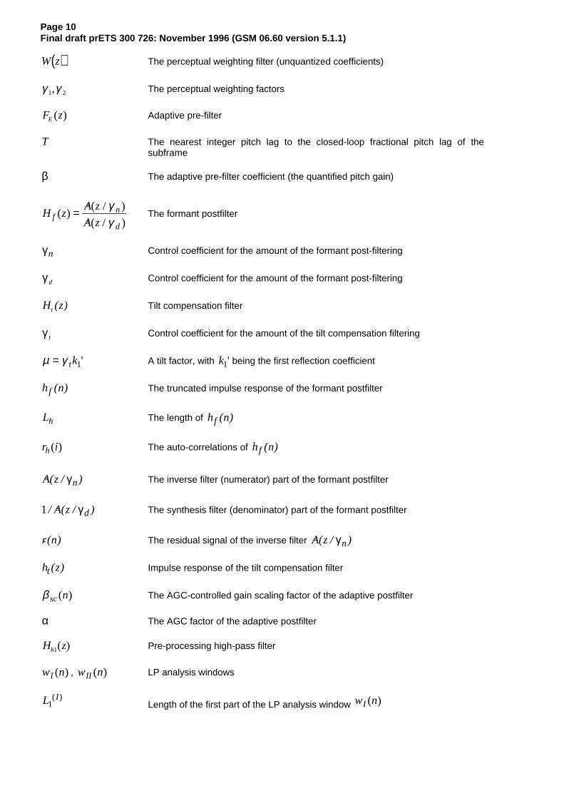
( )W z The perceptual weighting filter (unquantized coefficients)
γ γ1 2, The perceptual weighting factors
F zE ( ) Adaptive pre-filter
T The nearest integer pitch lag to the closed-loop fractional pitch lag of thesubframe
β The adaptive pre-filter coefficient (the quantified pitch gain)
H zA z
A zf
n
d
( )�( / )�( / )
= γγ
The formant postfilter
γ n Control coefficient for the amount of the formant post-filtering
γ d Control coefficient for the amount of the formant post-filtering
H zt ( ) Tilt compensation filter
γ t Control coefficient for the amount of the tilt compensation filtering
µ γ= tk1' A tilt factor, with k1' being the first reflection coefficient
h nf ( ) The truncated impulse response of the formant postfilter
Lh The length of h nf ( )
r ih( ) The auto-correlations of h nf ( )
� ( / )A z nγ The inverse filter (numerator) part of the formant postfilter
1/ � ( / )A z dγ The synthesis filter (denominator) part of the formant postfilter
�( )r n The residual signal of the inverse filter � ( / )A z nγ
h zt ( ) Impulse response of the tilt compensation filter
β sc n( ) The AGC-controlled gain scaling factor of the adaptive postfilter
α The AGC factor of the adaptive postfilter
H zh1( ) Pre-processing high-pass filter
w nI ( ) , w nII ( ) LP analysis windows
L I1( )
Length of the first part of the LP analysis window w nI ( )
Page 11Final draft prETS 300 726: November 1996 (GSM 06.60 version 5.1.1)
L I2
( )Length of the second part of the LP analysis window w nI ( )
L II1( )
Length of the first part of the LP analysis window w nII ( )
L II2
( )Length of the second part of the LP analysis window w nII ( )
r kac( ) The auto-correlations of the windowed speech s n' ( )
w ilag( ) Lag window for the auto-correlations (60 Hz bandwidth expansion)
f0 The bandwidth expansion in Hz
fs The sampling frequency in Hz
r kac' ( )The modified (bandwidth expanded) auto-correlations
( )E iLD The prediction error in the ith iteration of the Levinson algorithm
ki The ith reflection coefficient
aji( ) The jth direct form coefficient in the ith iteration of the Levinson algorithm
F z1' ( ) Symmetric LSF polynomial
F z2' ( ) Antisymmetric LSF polynomial
F z1 ( ) Polynomial ( )F z1′ with root z = −1 eliminated
F z2 ( ) Polynomial ( )F z2′ with root z = 1 eliminated
qi The line spectral pairs (LSPs) in the cosine domain
q An LSP vector in the cosine domain
�( )qin The quantified LSP vector at the ith subframe of the frame n
ω i The line spectral frequencies (LSFs)
T xm( ) A mth order Chebyshev polynomial
f i f i1 2( ), ( ) The coefficients of the polynomials F z1( ) and F z2( )
f i f i1 2' '( ), ( ) The coefficients of the polynomials ( )F z1
′ and ( )F z2′
f i( ) The coefficients of either F z1( ) or F z2( )
Page 12Final draft prETS 300 726: November 1996 (GSM 06.60 version 5.1.1)
C x( ) Sum polynomial of the Chebyshev polynomials
x Cosine of angular frequency ω
λ k Recursion coefficients for the Chebyshev polynomial evaluation
fi The line spectral frequencies (LSFs) in Hz
[ ]f t f f f= 1 2 10� The vector representation of the LSFs in Hz
z( )( )1 n , z( ) ( )2 n The mean-removed LSF vectors at frame n
r ( )( )1 n , r ( )( )2 n The LSF prediction residual vectors at frame n
p( )n The predicted LSF vector at frame n
� ( )( )r 2 1n− The quantified second residual vector at the past frame
�f k The quantified LSF vector at quantization index k
ELSP The LSP quantization error
w ii , , , ,= 1 10� LSP-quantization weighting factors
di The distance between the line spectral frequencies fi +1 and fi −1
h n( ) The impulse response of the weighted synthesis filter
Ok The correlation maximum of open-loop pitch analysis at delay k
O iti, , ,=1 3� The correlation maxima at delays t ii , , ,= 1 3�
( )M t ii i, , , ,=1 3� The normalized correlation maxima Mi and the corresponding delays
t ii , , ,= 1 3�
H z W zA z
A z A z( ) ( )
( / )�( ) ( / )
= γγ
1
2
The weighted synthesis filter
A z( / )γ1 The numerator of the perceptual weighting filter
1 2/ ( / )A z γ The denominator of the perceptual weighting filter
T1 The nearest integer to the fractional pitch lag of the previous (1st or 3rd)subframe
s n' ( ) The windowed speech signal
s nw( ) The weighted speech signal

Page 13Final draft prETS 300 726: November 1996 (GSM 06.60 version 5.1.1)
�( )s n Reconstructed speech signal
� ( )′s n The gain-scaled post-filtered signal
� ( )s nf Post-filtered speech signal (before scaling)
x n( ) The target signal for adaptive codebook search
x n2( ) , x2t The target signal for algebraic codebook search
res nLP( ) The LP residual signal
c n( ) The fixed codebook vector
v n( ) The adaptive codebook vector
y n v n h n( ) = ( ) ( )∗ The filtered adaptive codebook vector
y nk ( ) The past filtered excitation
u n( ) The excitation signal
( )�u n The emphasized adaptive codebook vector
�' ( )u n The gain-scaled emphasized excitation signal
Top The best open-loop lag
tmin Minimum lag search value
tmax Maximum lag search value
( )R k Correlation term to be maximized in the adaptive codebook search
b24 The FIR filter for interpolating the normalized correlation term ( )R k
( )R k t The interpolated value of ( )R k for the integer delay k and fraction t
b60 The FIR filter for interpolating the past excitation signal u n( ) to yield the
adaptive codebook vector v n( )
Ak Correlation term to be maximized in the algebraic codebook search at index k
Ck The correlation in the numerator of Ak at index k
EDk The energy in the denominator of Ak at index k
Page 14Final draft prETS 300 726: November 1996 (GSM 06.60 version 5.1.1)
d H x= t2 The correlation between the target signal ( )x n2 and the impulse response
( )h n , i.e., backward filtered target
H The lower triangular Toepliz convolution matrix with diagonal ( )h 0 and lower
diagonals ( ) ( )h h1 39, ,�
Φ = H Ht The matrix of correlations of ( )h n
d n( ) The elements of the vector d
φ( , )i j The elements of the symmetric matrix Φ
ck The innovation vector
C The correlation in the numerator of Ak
mi The position of the i th pulse
ϑ i The amplitude of the i th pulse
Np The number of pulses in the fixed codebook excitation
ED The energy in the denominator of Ak
( )res nLTP The normalized long-term prediction residual
b n( ) The sum of the normalized ( )d n vector and normalized long-term prediction
residual ( )res nLTP
s nb( ) The sign signal for the algebraic codebook search
d n' ( ) Sign extended backward filtered target
φ' ( , )i j The modified elements of the matrix Φ , including sign information
zt , ( )z n The fixed codebook vector convolved with h n( )
E n( ) The mean-removed innovation energy (in dB)
E The mean of the innovation energy
~( )E n The predicted energy
[ ]b b b b1 2 3 4 The MA prediction coefficients
�( )R k The quantified prediction error at subframe k

Page 15Final draft prETS 300 726: November 1996 (GSM 06.60 version 5.1.1)
EI The mean innovation energy
R n( ) The prediction error of the fixed-codebook gain quantization
EQ The quantization error of the fixed-codebook gain quantization
e n( ) The states of the synthesis filter 1/ �( )A z
e nw( ) The perceptually weighted error of the analysis-by-synthesis search
η The gain scaling factor for the emphasized excitation
gc The fixed-codebook gain
gc' The predicted fixed-codebook gain
�gc The quantified fixed codebook gain
gp The adaptive codebook gain
�gp The quantified adaptive codebook gain
γ gc c cg g= / ' A correction factor between the gain gc and the estimated one gc'
�γ gc The optimum value for γ gc
γ sc Gain scaling factor
3.3 Abbreviations
For the purposes of this ETS the following abbreviations apply. Further GSM related abbreviations may befound in GSM 01.04 [1].
ACELP Algebraic Code Excited Linear PredictionAGC Adaptive Gain ControlCELP Code Excited Linear PredictionFIR Finite Impulse ResponseISPP Interleaved Single-Pulse PermutationLP Linear PredictionLPC Linear Predictive CodingLSF Line Spectral FrequencyLSP Line Spectral PairLTP Long Term Predictor (or Long Term Prediction)MA Moving Average
4 Outline description
This ETS is structured as follows:
Section 4.1 contains a functional description of the audio parts including the A/D and D/A functions.Section 4.2 describes the conversion between 13-bit uniform and 8-bit A-law samples. Sections 4.3 and4.4 present a simplified description of the principles of the GSM EFR encoding and decoding processrespectively. In section 4.5, the sequence and subjective importance of encoded parameters are given.

Page 16Final draft prETS 300 726: November 1996 (GSM 06.60 version 5.1.1)
Section 5 presents the functional description of the GSM EFR encoding, whereas section 6 describes thedecoding procedures. Section 7 describes variables, constants and tables of the C-code of the GSM EFRcodec.
4.1 Functional description of audio parts
The analogue-to-digital and digital-to-analogue conversion will in principle comprise the followingelements:
1) Analogue to uniform digital PCM− microphone;− input level adjustment device;− input anti-aliasing filter;− sample-hold device sampling at 8 kHz;− analogue-to-uniform digital conversion to 13-bit representation.
The uniform format shall be represented in two's complement.
2) Uniform digital PCM to analogue− conversion from 13-bit/8 kHz uniform PCM to analogue;− a hold device;− reconstruction filter including x/sin( x ) correction;− output level adjustment device;− earphone or loudspeaker.
In the terminal equipment, the A/D function may be achieved either
− by direct conversion to 13-bit uniform PCM format;
− or by conversion to 8-bit/A-law compounded format, based on a standard A-law codec/filteraccording to ITU-T Recommendations G.711 [8] and G.714, followed by the 8-bit to 13-bitconversion as specified in section 4.2.1.
For the D/A operation, the inverse operations take place.
In the latter case it should be noted that the specifications in ITU-T G.714 (superseded by G.712) areconcerned with PCM equipment located in the central parts of the network. When used in the terminalequipment, this ETS does not on its own ensure sufficient out-of-band attenuation. The specification ofout-of-band signals is defined in GSM 03.50 [2] in section 2.
4.2 Preparation of speech samples
The encoder is fed with data comprising of samples with a resolution of 13 bits left justified in a 16-bitword. The three least significant bits are set to '0'. The decoder outputs data in the same format. Outsidethe speech codec further processing must be applied if the traffic data occurs in a different representation.
4.2.1 PCM format conversion
The conversion between 8-bit A-Law compressed data and linear data with 13-bit resolution at the speechencoder input shall be as defined in ITU-T Rec. G.711 [8].
ITU-T Rec. G.711 [8] specifies the A-Law to linear conversion and vice versa by providing table entries.Examples on how to perform the conversion by fixed-point arithmetic can be found in ITU-T Rec. G.726[9]. Section 4.2.1 of G.726 [9] describes A-Law to linear expansion and section 4.2.7 of G.726 [9] providesa solution for linear to A-Law compression.
4.3 Principles of the GSM enhanced full rate speech encoder
The codec is based on the code-excited linear predictive (CELP) coding model. A 10th order linearprediction (LP), or short-term, synthesis filter is used which is given by

Page 17Final draft prETS 300 726: November 1996 (GSM 06.60 version 5.1.1)
H zA z a z
i
mi
i( )
� ( ) �
,= =+
=−∑
1 1
11
(1)
where � , , , ,a i mi = 1� are the (quantified) linear prediction (LP) parameters, and m= 10 is the predictororder. The long-term, or pitch, synthesis filter is given by
1 11B z g zp
T( ),=
− − (2)
where T is the pitch delay and gp is the pitch gain. The pitch synthesis filter is implemented using the
so-called adaptive codebook approach.
The CELP speech synthesis model is shown in figure 2. In this model, the excitation signal at the input ofthe short-term LP synthesis filter is constructed by adding two excitation vectors from adaptive and fixed(innovative) codebooks. The speech is synthesized by feeding the two properly chosen vectors from thesecodebooks through the short-term synthesis filter. The optimum excitation sequence in a codebook ischosen using an analysis-by-synthesis search procedure in which the error between the original andsynthesized speech is minimized according to a perceptually weighted distortion measure.
The perceptual weighting filter used in the analysis-by-synthesis search technique is given by
W zA z
A z( )
( / )
( / ),= γ
γ1
2(3)
where ( )A z is the unquantized LP filter and 0 12 1< < ≤γ γ are the perceptual weighting factors. The
values γ 1 0 9= . and γ 2 0 6= . are used. The weighting filter uses the unquantized LP parameters whilethe formant synthesis filter uses the quantified ones.
The coder operates on speech frames of 20 ms corresponding to 160 samples at the sampling frequencyof 8000 sample/s. At each 160 speech samples, the speech signal is analysed to extract the parametersof the CELP model (LP filter coefficients, adaptive and fixed codebooks' indices and gains). Theseparameters are encoded and transmitted. At the decoder, these parameters are decoded and speech issynthesized by filtering the reconstructed excitation signal through the LP synthesis filter.

Page 18Final draft prETS 300 726: November 1996 (GSM 06.60 version 5.1.1)
The signal flow at the encoder is shown in figure 3. LP analysis is performed twice per frame. The twosets of LP parameters are converted to line spectrum pairs (LSP) and jointly quantified using split matrixquantization (SMQ) with 38 bits. The speech frame is divided into 4 subframes of 5 ms each (40samples). The adaptive and fixed codebook parameters are transmitted every subframe. The two sets ofquantified and unquantized LP filters are used for the second and fourth subframes while in the first andthird subframes interpolated LP filters are used (both quantified and unquantized). An open-loop pitch lagis estimated twice per frame (every 10 ms) based on the perceptually weighted speech signal.
Then the following operations are repeated for each subframe:
The target signal x n( ) is computed by filtering the LP residual through the weighted synthesis filter
W z H z( ) ( ) with the initial states of the filters having been updated by filtering the error betweenLP residual and excitation (this is equivalent to the common approach of subtracting the zero inputresponse of the weighted synthesis filter from the weighted speech signal).
The impulse response, h n( ) of the weighted synthesis filter is computed.
Closed-loop pitch analysis is then performed (to find the pitch lag and gain), using the target x n( )and impulse response h n( ) , by searching around the open-loop pitch lag. Fractional pitch with1/6th of a sample resolution is used. The pitch lag is encoded with 9 bits in the first and thirdsubframes and relatively encoded with 6 bits in the second and fourth subframes.
The target signal x n( ) is updated by removing the adaptive codebook contribution (filtered
adaptive codevector), and this new target, x n2( ) , is used in the fixed algebraic codebook search(to find the optimum innovation). An algebraic codebook with 35 bits is used for the innovativeexcitation.
The gains of the adaptive and fixed codebook are scalar quantified with 4 and 5 bits respectively(with moving average (MA) prediction applied to the fixed codebook gain).
Finally, the filter memories are updated (using the determined excitation signal) for finding the targetsignal in the next subframe.
The bit allocation of the codec is shown in table 1. In each 20 ms speech frame, 244 bits are produced,corresponding to a bit rate of 12.2 kbit/s. More detailed bit allocation is available in table 6. Note that themost significant bits (MSB) are always sent first.
Table 1: Bit allocation of the 12.2 kbit/s coding algorithm for 20 ms frame.
Parameter 1st & 3rd subframes 2nd & 4th subframes total per frame
2 LSP sets 38
Pitch delay 9 6 30Pitch gain 4 4 16
Algebraic code 35 35 140Codebook gain 5 5 20
Total 244
4.4 Principles of the GSM enhanced full rate speech decoder
The signal flow at the decoder is shown in figure 4. At the decoder, the transmitted indices are extractedfrom the received bitstream. The indices are decoded to obtain the coder parameters at eachtransmission frame. These parameters are the two LSP vectors, the 4 fractional pitch lags, the 4innovative codevectors, and the 4 sets of pitch and innovative gains. The LSP vectors are converted to theLP filter coefficients and interpolated to obtain LP filters at each subframe. Then, at each 40-samplesubframe:

Page 19Final draft prETS 300 726: November 1996 (GSM 06.60 version 5.1.1)
- the excitation is constructed by adding the adaptive and innovative codevectors scaled by theirrespective gains.
- the speech is reconstructed by filtering the excitation through the LP synthesis filter.
Finally, the reconstructed speech signal is passed through an adaptive postfilter.
4.5 Sequence and subjective importance of encoded parameters
The encoder will produce the output information in a unique sequence and format, and the decoder mustreceive the same information in the same way. In table 6, the sequence of output bits s1 to s244 and thebit allocation for each parameter is shown.
The different parameters of the encoded speech and their individual bits have unequal importance withrespect to subjective quality. Before being submitted to the channel encoding function the bits have to berearranged in the sequence of importance as given in table6 in 05.03 [3].
5 Functional description of the encoder
In this section, the different functions of the encoder represented in figure 3 are described.
5.1 Pre-processing
Two pre-processing functions are applied prior to the encoding process: high-pass filtering and signaldown-scaling.
Down-scaling consists of dividing the input by a factor of 2 to reduce the possibility of overflows in thefixed-point implementation.
The high-pass filter serves as a precaution against undesired low frequency components. A filter with acut off frequency of 80 Hz is used, and it is given by
H zz z
z zh1
1 2
1 2
0 92727435 18544941 0 927274351 19059465 0 9114024
( ). . .
. ..= − +
− +
− −
− − (4)
Down-scaling and high-pass filtering are combined by dividing the coefficients at the numerator ofH zh1( ) by 2.
5.2 Linear prediction analysis and quantization
Short-term prediction, or linear prediction (LP), analysis is performed twice per speech frame using theauto-correlation approach with 30 ms asymmetric windows. No lookahead is used in the auto-correlationcomputation.
The auto-correlations of windowed speech are converted to the LP coefficients using the Levinson-Durbinalgorithm. Then the LP coefficients are transformed to the Line Spectral Pair (LSP) domain forquantization and interpolation purposes. The interpolated quantified and unquantized filter coefficients areconverted back to the LP filter coefficients (to construct the synthesis and weighting filters at eachsubframe).
5.2.1 Windowing and auto-correlation computation
LP analysis is performed twice per frame using two different asymmetric windows. The first window has itsweight concentrated at the second subframe and it consists of two halves of Hamming windows withdifferent sizes. The window is given by

Page 20Final draft prETS 300 726: November 1996 (GSM 06.60 version 5.1.1)
w n
n
Ln L
n L
Ln L L L
I
II
I
II I I
( )
. .46 , , , ,
. .46( )
, , , .
( )( )
( )
( )( ) ( ) ( )
=−
−
= −
+ −−
= + −
0 54 01
0 1
0 54 01
1
11
1
21 1 2
cos
cos
π
π
�
�
(5)
The values L I1 160( ) = and L I
2 80( ) = are used. The second window has its weight concentrated atthe fourth subframe and it consists of two parts: the first part is half a Hamming window and the secondpart is a quarter of a cosine function cycle. The window is given by:
w n
n
Ln L
n L
Ln L L L
II
IIII
II
IIII II II
( )
. .46 , , , ,
( ), , ,
( )( )
( )
( )( ) ( ) ( )
=−
−
= −
−−
= + −
0 54 02
2 10 1
2
4 11
11
1
21 1 2
cos
cos
π
π
�
�
(6)
where the values L II1 232( ) = and L II
2 8( ) = are used.
Note that both LP analyses are performed on the same set of speech samples. The windows are appliedto 80 samples from past speech frame in addition to the 160 samples of the present speech frame. Nosamples from future frames are used (no lookahead). A diagram of the two LP analysis windows isdepicted below.
2 0 m s5 m s
fram e (16 0 sam p les) su b fra m e(40 sa m p les )
fr a m e n -1 fra m e n
t
Iw (n )
IIw (n )
Figure 1: LP analysis windows
The auto-correlations of the windowed speech s n n' ( ), , ,= 0 239� , are computed by
r k s n s n k kacn k
( ) ' ( ) ' ( ) , , , ,= − ==∑239
0 10 � (7)
and a 60 Hz bandwidth expansion is used by lag windowing the auto-correlations using the window
w if i
filag
s( ) , , , ,= −
=exp 1
2
21 100
2π
� (8)
where f0 60= Hz is the bandwidth expansion and fs = 8000 Hz is the sampling frequency. Further,
rac( )0 is multiplied by the white noise correction factor 1.0001 which is equivalent to adding a noise floor
at -40 dB.

Page 21Final draft prETS 300 726: November 1996 (GSM 06.60 version 5.1.1)
5.2.2 Levinson-Durbin algorithm
The modified auto-correlations r rac ac' ( ) . ( )0 1 0001 0= and r k r k w k kac ac lag' ( ) ( ) ( ), , ,= = 1 10� are
used to obtain the direct form LP filter coefficients a kk , , , ,= 1 10� by solving the set of equations.
( )a r i k r i ik ack
ac' ' ( ) , , , .− = − ==
∑1
10
1 10 � (9)
The set of equations in (9) is solved using the Levinson-Durbin algorithm. This algorithm uses thefollowing recursion:
[ ]
E ria
k a r i j E i
a kj i
a a k a
E i k E i
LD ac
i
i ji
acj
iLD
ii
i
ji
ji
i i ji
LD i LD
( ) ' ( )
' ( ) / ( )
( ) ( ) ( )
( )
( )
( )
( ) ( ) ( )
0 01 10
1
1
1 1
1 1
01
10
1
1 1
2
==
=
= − − −
== −
= +
= − −
−
−=−
−−−
∑
for to do
for to do
end end
The final solution is given as a a jj j= =( ) , , ,10 1 10� .
The LP filter coefficients are converted to the line spectral pair (LSP) representation for quantization andinterpolation purposes. The conversions to the LSP domain and back to the LP filter coefficient domainare described in the next section.
5.2.3 LP to LSP conversion
The LP filter coefficients a kk , , ,= 1 10� , are converted to the line spectral pair (LSP) representation forquantization and interpolation purposes. For a 10th order LP filter, the LSPs are defined as the roots of thesum and difference polynomials
F z A z z A z111 1' ( ) ( ) ( )= + − − (10)
and
F z A z z A z211 1' ( ) ( ) ( )= − − − , (11)
respectively. The polynomial F z1' ( ) and F z2
' ( ) are symmetric and anti-symmetric, respectively. It can
be proven that all roots of these polynomials are on the unit circle and they alternate each other. F z1' ( )
has a root z = − =1 ( )ω π and F z2' ( ) has a root z = =1 0( )ω . To eliminate these two roots, we
define the new polynomials
F z F z z1 111( ) ( ) / ( )'= + − (12)

Page 22Final draft prETS 300 726: November 1996 (GSM 06.60 version 5.1.1)
and
F z F z z2 211( ) ( ) / ( )'= − − . (13)
Each polynomial has 5 conjugate roots on the unit circle ( )e j i± ω , therefore, the polynomials can be written
as
( )F z q z zii
11 2
1 3 9
1 2( ), , ,
= − +− −
=∏�
(14)
and
( )F z q z zii
21 2
2 4 10
1 2( ), , ,
= − +− −
=∏�
, (15)
where ( )qi i= cos ω with ω i being the line spectral frequencies (LSF) and they satisfy the ordering
property 0 1 2 10< < < < <ω ω ω π� . We refer to q i as the LSPs in the cosine domain.
Since both polynomials F z1( ) and F z2( ) are symmetric only the first 5 coefficients of each polynomial
need to be computed. The coefficients of these polynomials are found by the recursive relations (for i = 0to 4)
f i a a f i
f i a a f ii m i
i m i
1 1 1
2 1 2
1
1
( ) ( ),
( ) ( )
+ = + −+ = − +
+ −
+ −
,(16)
where m= 10 is the predictor order.
The LSPs are found by evaluating the polynomials F z1( ) and F z2( ) at 60 points equally spacedbetween 0 and π and checking for sign changes. A sign change signifies the existence of a root and thesign change interval is then divided 4 times to better track the root. The Chebyshev polynomials are used
to evaluate F z1( ) and F z2( ) . In this method the roots are found directly in the cosine domain { }qi . The
polynomials F z1( ) or F z2( ) evaluated at z ej= ω can be written as
F e C xj( ) ( ),ω ω= −2 5
with
C x T x f T x f T x f T x f T x f( ) ( ) ( ) ( ) ( ) ( ) ( ) ( ) ( ) ( ) ( ) /= + + + + +5 4 3 2 11 2 3 4 5 2, (17)
where T x mm( ) cos( )= ω is the mth order Chebyshev polynomial, and f i i( ), , , , = 1 5� are the
coefficients of either F z1( ) or F z2( ) , computed using the equations in (16). The polynomial C x( ) is
evaluated at a certain value of x = cos( )ω using the recursive relation:
for down to end
kx f k
C x x f
k k k
=− + −
= − +
= + +
4 12 5
5 2
1 2
1 2
λ λ λ
λ λ
( )
( ) ( ) / ,
Page 23Final draft prETS 300 726: November 1996 (GSM 06.60 version 5.1.1)
with initial values λ5 1= and λ6 0= . The details of the Chebyshev polynomial evaluation method are
found in P. Kabal and R.P. Ramachandran [6].
5.2.4 LSP to LP conversion
Once the LSPs are quantified and interpolated, they are converted back to the LP coefficient domain
{ }ak . The conversion to the LP domain is done as follows. The coefficients of F z1( ) or F z2( ) are found
by expanding equations (14) and (15) knowing the quantified and interpolated LSPs q ii , = , ,1 10� . The
following recursive relation is used to compute f i1( )
for to
for down to
end
end
i
f i q f i f i
j i
f j f j q f j f j
i
i
== − − + −= −
= − − + −
−
−
1 5
2 1 2 2
1 1
2 1 2
1 2 1 1 1
1 1 2 1 1 1
( ) ( ) ( )
( ) ( ) ( ) ( )
with initial values ( )f1 0 1= and ( )f1 1 0− = . The coefficients ( )f i2 are computed similarly by replacing
q i2 1− by q i2 .
Once the coefficients f i1( ) and f i2( ) are found, F z1( ) and F z2( ) are multiplied by 1 1+ −z and
1 1− −z , respectively, to obtain F z1' ( ) and F z2
' ( ) ; that is
f i f i f i i
f i f i f i i
1 1 1
2 2 2
1 1 5
1 1 5
'
'
( ) ( ) ( ) , , , ,
( ) ( ) ( ) , , , .
= + − =
= − − =
�
�
(18)
Finally the LP coefficients are found by
af i f i i
f i f i ii = + =
− − − =
0 5 0 5 1 5
0 5 11 0 5 11 6 101 2
1 2
. ( ) . ( ) , , , ,
. ( ) . ( ) , , , .
' '
' '
�
�
(19)
This is directly derived from the relation ( )A z F z F z( ) ( ) ( ) /' '= +1 2 2 , and considering the fact that
F z1' ( ) and F z2
' ( ) are symmetric and anti-symmetric polynomials, respectively.
5.2.5 Quantization of the LSP coefficients
The two sets of LP filter coefficients per frame are quantified using the LSP representation in thefrequency domain; that is
( )ff
q iis
i= =2
1 10π
arccos , , , ,� (20)
where fi are the line spectral frequencies (LSF) in Hz [0,4000] and fs=8000 is the sampling frequency.
The LSF vector is given by [ ]f t f f f= 1 2 10� , with t denoting transpose.

Page 24Final draft prETS 300 726: November 1996 (GSM 06.60 version 5.1.1)
A 1st order MA prediction is applied, and the two residual LSF vectors are jointly quantified using split
matrix quantization (SMQ). The prediction and quantization are performed as follows. Let z( ) ( )1 n and
z( ) ( )2 n denote the mean-removed LSF vectors at frame n . The prediction residual vectors r ( ) ( )1 n
and r ( ) ( )2 n are given by
r z p
r z p
( ) ( )
( ) ( )
( ) ( ) ( ),
( ) ( ) ( ),
1 1
2 2
n n n
n n n
= −
= −
and
(21)
where p( )n is the predicted LSF vector at frame n . First order moving-average (MA) prediction is used
where
( )p r( ) . �( )n n= −0 65 12 , (22)
where � ( )( )r 2 1n− is the quantified second residual vector at the past frame.
The two LSF residual vectors r ( )1 and r ( )2 are jointly quantified using split matrix quantization (SMQ).
The matrix ( )r r( ) ( )1 2 is split into 5 submatrices of dimension 2 x 2 (two elements from each vector). For
example, the first submatrix consists of the elements r r r11
21
12( ) ( ) ( ), , , and r2
2( ) . The 5 submatrices are
quantified with 7, 8, 8+1, 8, and 6 bits, respectively. The third submatrix uses a 256-entry signedcodebook (8-bit index plus 1-bit sign).
A weighted LSP distortion measure is used in the quantization process. In general, for an input LSP vector
f and a quantified vector at index k , �f k , the quantization is performed by finding the index k whichminimizes
[ ]E f w f wLSP i i ik
ii
= −=∑ � .
1
10 2
(23)
The weighting factors w ii , , ,=1 10� , are given by
w d d
d
i i i
i
= − <
= − −
33471547
450450
180 8
1050450
..
,
..
( )
for
otherwise,(24)
where d f fi i i= −+ −1 1 with f0 0= and f11 4000= . Here, two sets of weighting coefficients are
computed for the two LSF vectors. In the quantization of each submatrix, two weighting coefficients fromeach set are used with their corresponding LSFs.
5.2.6 Interpolation of the LSPs
The two sets of quantified (and unquantized) LP parameters are used for the second and fourthsubframes whereas the first and third subframes use a linear interpolation of the parameters in the
adjacent subframes. The interpolation is performed on the LSPs in the q domain. Let �( )q4n be the LSP
vector at the 4th subframe of the present frame n , �( )q2n be the LSP vector at the 2nd subframe of the

Page 25Final draft prETS 300 726: November 1996 (GSM 06.60 version 5.1.1)
present frame n , and �( )q41n− the LSP vector at the 4th subframe of the past frame n−1. The
interpolated LSP vectors at the 1st and 3rd subframes are given by
� . � . � ,
� . � . � .
( ) ( ) ( )
( ) ( ) ( )
q q q
q q q
1 41
2
3 2 4
0 5 0 5
0 5 0 5
n n n
n n n
= +
= +
−(25)
The interpolated LSP vectors are used to compute a different LP filter at each subframe (both quantifiedand unquantized coefficients) using the LSP to LP conversion method described in section 5.2.4.
5.3 Open-loop pitch analysis
Open-loop pitch analysis is performed twice per frame (each 10 ms) to find two estimates of the pitch lagin each frame. This is done in order to simplify the pitch analysis and confine the closed-loop pitch searchto a small number of lags around the open-loop estimated lags.
Open-loop pitch estimation is based on the weighted speech signal s nw( ) which is obtained by filtering
the input speech signal through the weighting filter W zA z
A z( )
( / )
( / )= γ
γ1
2. That is, in a subframe of size L ,
the weighted speech is given by
s n s n a s n i a s n i n Lw ii
ii
i
iw( ) ( ) ( ) ( ), , , .= + − − − = −
= =∑ ∑γ γ1
1
10
21
10
0 1� (26)
Open-loop pitch analysis is performed as follows. In the first step, 3 maxima of the correlation
O s n s n kk w wn
= −=∑ ( ) ( )
0
79
(27)
are found in the three ranges:
i
i
i
===
3
2
1
:
:
:
18 35
36 71
72 143
, , ,
, , ,
, , .
�
�
�
The retained maxima O iti, , ,=1 3� , are normalized by dividing by s n t iw in
2 ( ),− =∑ 1, ,3� ,
respectively. The normalized maxima and corresponding delays are denoted by ( )M t ii i, , , ,=1 3� . The
winner, Top , among the three normalized correlations is selected by favouring the delays with the values
in the lower range. This is performed by weighting the normalized correlations corresponding to the longerdelays. The best open-loop delay Top is determined as follows:

Page 26Final draft prETS 300 726: November 1996 (GSM 06.60 version 5.1.1)
( )( )
( )
( )( )
T t
M T M
if M M T
M T MT t
end
if M M T
M T MT t
end
op
op
op
op
op
op
op
op
==
>
==
>
==
1
1
2
2
2
3
3
3
0 85
0 85
.
.
This procedure of dividing the delay range into 3 sections and favouring the lower sections is used toavoid choosing pitch multiples.
5.4 Impulse response computation
The impulse response, h n( ) , of the weighted synthesis filter
[ ]H z W z A z A z A z( ) ( ) ( / ) / �( ) ( / )= γ γ1 2 is computed each subframe. This impulse response is
needed for the search of adaptive and fixed codebooks. The impulse response h n( ) is computed by
filtering the vector of coefficients of the filter A z( / )γ1 extended by zeros through the two filters 1/ �( )A zand 1 2/ ( / )A z γ .
5.5 Target signal computation
The target signal for adaptive codebook search is usually computed by subtracting the zero input
response of the weighted synthesis filter [ ]H z W z A z A z A z( ) ( ) ( / ) / �( ) ( / )= γ γ1 2 from the weighted
speech signal s nw( ) . This is performed on a subframe basis.
An equivalent procedure for computing the target signal, which is used in this standard, is the filtering of
the LP residual signal res nLP( ) through the combination of synthesis filter 1/ �( )A z and the weighting
filter A z A z( / ) / ( / )γ γ1 2 . After determining the excitation for the subframe, the initial states of these
filters are updated by filtering the difference between the LP residual and excitation. The memory updateof these filters is explained in section 5.9.
The residual signal res nLP( ) which is needed for finding the target vector is also used in the adaptive
codebook search to extend the past excitation buffer. This simplifies the adaptive codebook searchprocedure for delays less than the subframe size of 40 as will be explained in the next section. The LPresidual is given by
res n s n a s n iLP ii
( ) ( ) � ( ).= + −=∑
1
10
(28)
5.6 Adaptive codebook search
Adaptive codebook search is performed on a subframe basis. It consists of performing closed-loop pitchsearch, and then computing the adaptive codevector by interpolating the past excitation at the selectedfractional pitch lag.
Page 27Final draft prETS 300 726: November 1996 (GSM 06.60 version 5.1.1)
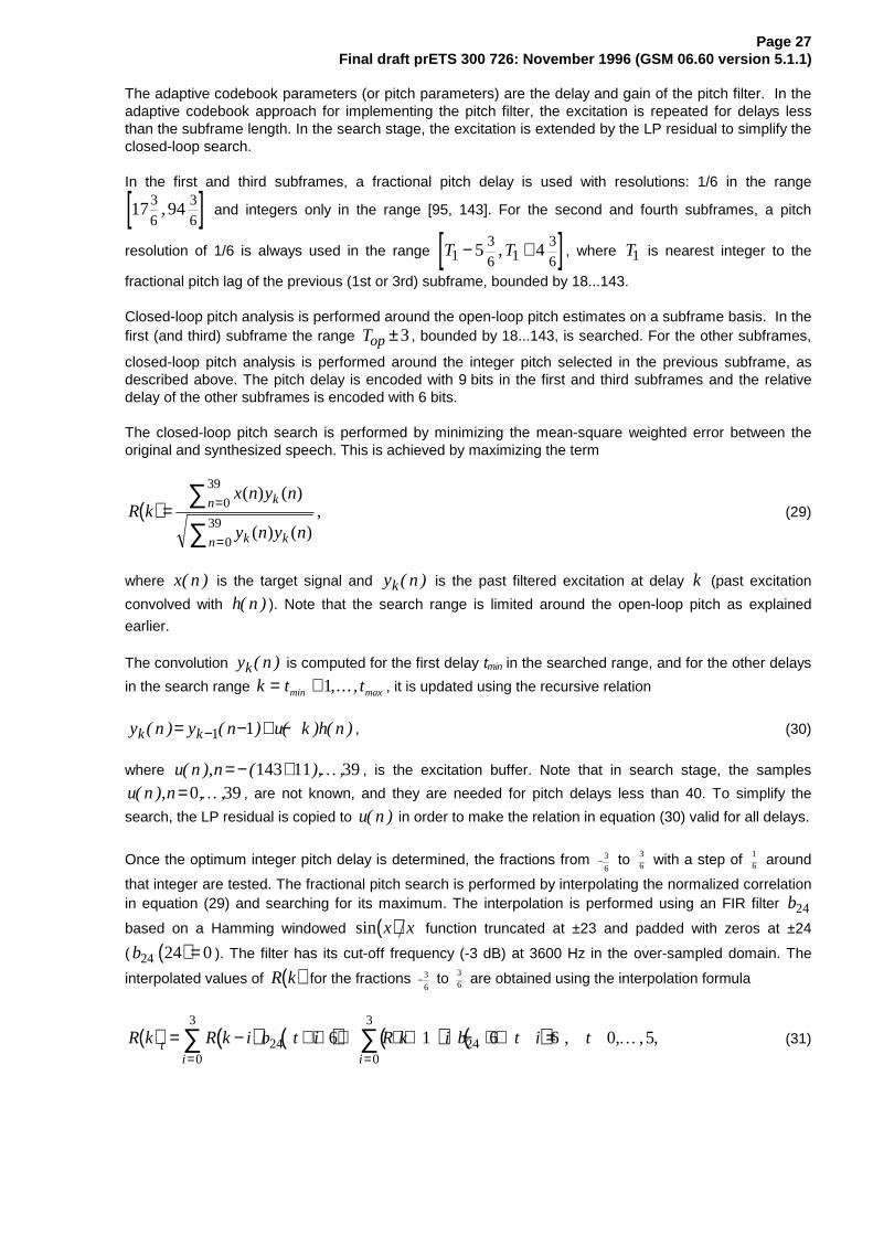
The adaptive codebook parameters (or pitch parameters) are the delay and gain of the pitch filter. In theadaptive codebook approach for implementing the pitch filter, the excitation is repeated for delays lessthan the subframe length. In the search stage, the excitation is extended by the LP residual to simplify theclosed-loop search.
In the first and third subframes, a fractional pitch delay is used with resolutions: 1/6 in the range
[ ]17 943
6
3
6, and integers only in the range [95, 143]. For the second and fourth subframes, a pitch
resolution of 1/6 is always used in the range [ ]T T13
6 13
65 4− +, , where T1 is nearest integer to the
fractional pitch lag of the previous (1st or 3rd) subframe, bounded by 18...143.
Closed-loop pitch analysis is performed around the open-loop pitch estimates on a subframe basis. In thefirst (and third) subframe the range Top ±3, bounded by 18...143, is searched. For the other subframes,
closed-loop pitch analysis is performed around the integer pitch selected in the previous subframe, asdescribed above. The pitch delay is encoded with 9 bits in the first and third subframes and the relativedelay of the other subframes is encoded with 6 bits.
The closed-loop pitch search is performed by minimizing the mean-square weighted error between theoriginal and synthesized speech. This is achieved by maximizing the term
( )R kx n y n
y n y n
kn
k kn
= =
=
∑∑
( ) ( )
( ) ( ),0
39
0
39(29)
where x n( ) is the target signal and y nk( ) is the past filtered excitation at delay k (past excitation
convolved with h n( ) ). Note that the search range is limited around the open-loop pitch as explained
earlier.
The convolution y nk( ) is computed for the first delay tmin in the searched range, and for the other delays
in the search range k t t= +min max,...,1 , it is updated using the recursive relation
y n y n u k h nk k( ) ( ) ( ) ( )= − + −−1 1 , (30)
where u n n( ), ( ), ,= − +143 11 39� , is the excitation buffer. Note that in search stage, the samples
u n n( ), , ,=0 39� , are not known, and they are needed for pitch delays less than 40. To simplify the
search, the LP residual is copied to u n( ) in order to make the relation in equation (30) valid for all delays.
Once the optimum integer pitch delay is determined, the fractions from − 3
6 to 3
6 with a step of 16 around
that integer are tested. The fractional pitch search is performed by interpolating the normalized correlationin equation (29) and searching for its maximum. The interpolation is performed using an FIR filter b24
based on a Hamming windowed ( )sin x x function truncated at ±23 and padded with zeros at ±24
( ( )b24 24 0= ). The filter has its cut-off frequency (-3 dB) at 3600 Hz in the over-sampled domain. The
interpolated values of ( )R k for the fractions − 3
6 to 3
6 are obtained using the interpolation formula
( ) ( ) ( ) ( ) ( )R k R k i b t i R k i b t i tti i
= − + ⋅ + + + − + ⋅ == =∑ ∑24
0
3
0
3
246 1 6 6 0 5, , , ,� (31)

Page 28Final draft prETS 300 726: November 1996 (GSM 06.60 version 5.1.1)
where t = 0 5, ,� corresponds to the fractions 0, 1
6,
2
6, 3
6 , −2
6, and −
1
6, respectively. Note that it is
necessary to compute the correlation terms in equation (29) using a range t tmin max, ,− +4 4 to allow for
the proper interpolation.
Once the fractional pitch lag is determined, the adaptive codebook vector v n( ) is computed by
interpolating the past excitation signal u n( ) at the given integer delay k and phase (fraction) t
( ) ( ) ( ) ( ) ( )v n u n k i b t i u n k i b t i n ti i
= − − + ⋅ + − + + − + ⋅ = == =∑ ∑60
0
9
0
9
606 1 6 6 0 39 0 5, , , , , , .� � (32)
The interpolation filter b60 is based on a Hamming windowed ( )sin x x function truncated at ±59 and
padded with zeros at ±60 ( ( )b60 60 0= ). The filter has a cut-off frequency (-3 dB) at 3600 Hz in the over-
sampled domain.
The adaptive codebook gain is then found by
gx n y n
y n y np
n
n
= ≤ ≤=
=
∑∑
( ) ( )
( ) ( ), . ,0
39
0
3912bounded by 0 gp (33)
where y n v n h n( ) ( ) ( )= ∗ is the filtered adaptive codebook vector (zero state response of H z W z( ) ( )to v n( ) ).
The computed adaptive codebook gain is quantified using 4-bit non-uniform scalar quantization in therange [0.0,1.2].
5.7 Algebraic codebook structure and search
The algebraic codebook structure is based on interleaved single-pulse permutation (ISPP) design. In thiscodebook, the innovation vector contains 10 non-zero pulses. All pulses can have the amplitudes +1 or -1.The 40 positions in a subframe are divided into 5 tracks, where each track contains two pulses, as shownin table 2.
Table 2: Potential positions of individual pulses in the algebraic codebook.
Track Pulse positions1 i0, i5 0, 5, 10, 15, 20, 25, 30, 352 i1, i6 1, 6, 11, 16, 21, 26, 31, 363 i2, i7 2, 7, 12, 17, 22, 27, 32, 374 i3, i8 3, 8, 13, 18, 23, 28, 33, 385 i4, i9 4, 9, 14, 19, 24, 29, 34, 39
Pulse positionsi0, i5 0, 5, 10, 15, 20, 25, 30, 35i1, i6 1, 6, 11, 16, 21, 26, 31, 36i2, i7 2, 7, 12, 17, 22, 27, 32, 37i3, i8 3, 8, 13, 18, 23, 28, 33, 38i4, i9 4, 9, 14, 19, 24, 29, 34, 39
Each two pulse positions in one track are encoded with 6 bits (total of 30 bits, 3 bits for the position ofevery pulse), and the sign of the first pulse in the track is encoded with 1 bit (total of 5 bits).

Page 29Final draft prETS 300 726: November 1996 (GSM 06.60 version 5.1.1)
For two pulses located in the same track, only one sign bit is needed. This sign bit indicates the sign of thefirst pulse. The sign of the second pulse depends on its position relative to the first pulse. If the position ofthe second pulse is smaller, then it has opposite sign, otherwise it has the same sign than in the firstpulse.
All the 3-bit pulse positions are Gray coded in order to improve robustness against channel errors. Thisgives a total of 35 bits for the algebraic code.
The algebraic codebook is searched by minimizing the mean square error between the weighted inputspeech and the weighted synthesized speech. The target signal used in the closed-loop pitch search isupdated by subtracting the adaptive codebook contribution. That is
x n x n g y n np2 0 39( ) ( ) � ( ), , , ,= − = � (34)
where y n v n h n( ) ( ) ( )= ∗ is the filtered adaptive codebook vector and �gp is the quantified adaptive
codebook gain. If ck is the algebraic codevector at index k , then the algebraic codebook is searched by
maximizing the term
( ) ( )A
C
Ekk
Dk
tk
kt
k
= =2 2
d c
c cΦ, (35)
where d H x= t2 is the correlation between the target signal ( )x n2 and the impulse response ( )h n , H
is a the lower triangular Toepliz convolution matrix with diagonal ( )h 0 and lower diagonals
( ) ( )h h1 39, ,� , and Φ = H Ht is the matrix of correlations of ( )h n . The vector d (backward filtered
target) and the matrix Φ are computed prior to the codebook search. The elements of the vector d arecomputed by
d n x i h i n ni n
( ) ( ) ( ), , , ,= − ==∑ 2
39
0 39� (36)
and the elements of the symmetric matrix Φ are computed by
φ( , ) ( ) ( ), ( ).i j h n i h n j j in j
= − − ≥=∑39
(37)
The algebraic structure of the codebooks allows for very fast search procedures since the innovationvector ck contains only a few nonzero pulses. The correlation in the numerator of Equation (35) is given
by
C d mi ii
Np
==
−
∑ϑ ( )0
1
, (38)
where mi is the position of the i th pulse, ϑ i is its amplitude, and Np is the number of pulses
(Np = 10 ). The energy in the denominator of equation (35) is given by
E m m m mD i i i j i jj i
N
i
N
i
N ppp
= += +
−
=
−
=
−
∑∑∑ φ ϑ ϑ φ( , ) ( , ).21
1
0
2
0
1
(39)

Page 30Final draft prETS 300 726: November 1996 (GSM 06.60 version 5.1.1)
To simplify the search procedure, the pulse amplitudes are preset by the mere quantization of anappropriate signal. In this case the signal b n( ) , which is a sum of the normalized d n( ) vector and
normalized long-term prediction residual ( )res nLTP
( ) ( )( ) ( )
( )( ) ( )
b nres n
res i res i
d n
d i d inLTP
LTP LTPi i
= + =
= =∑ ∑0
39
0
390 39, , , ,� (40)
is used. This is simply done by setting the amplitude of a pulse at a certain position equal to the sign ofb n( ) at that position. The simplification proceeds as follows (prior to the codebook search). First, the sign
signal [ ]s n b nb( ) ( )= sign and the signal d n d n s nb' ( ) ( ) ( )= are computed. Second, the matrix Φ is
modified by including the sign information; that is, φ φ' ( , ) ( ) ( ) ( , )i j s i s j i jb b= . The correlation in equation
(38) is now given by
C d mii
Np
==
−
∑ ' ( )0
1
(41)
and the energy in equation (39) is given by
E m m m mD i i i jj i
N
i
N
i
N ppp
= += +
−
=
−
=
−
∑∑∑φ φ' '( , ) ( , ).21
1
0
2
0
1
(42)
Having preset the pulse amplitudes, as explained above, the optimal pulse positions are determined usingan efficient non-exhaustive analysis-by-synthesis search technique. In this technique, the term in equation(35) is tested for a small percentage of position combinations.
First, for each of the five tracks the pulse positions with maximum absolute values of b n( ) are searched.From these the global maximum value for all the pulse positions is selected. The first pulse i0 is alwaysset into the position corresponding to the global maximum value.
Next, five iterations are carried out in which the position of pulse i1 is set to one of the five maxima in thetrack. The rest of the pulses are searched in pairs by sequentially searching each of the pulse pairs {i2,i3},{i4,i5}, {i6,i7} and {i8,i9} in nested loops. Every pulse has 8 possible positions, i.e., there are four 8x8-loops, resulting in 256 different combinations of pulse positions for each iteration.
In each iteration all the 9 pulse starting positions are cyclically shifted, so that the pulse pairs are changedand the pulse i1 is placed in a local maximum of a different track. The rest of the pulses are searched alsofor the other positions in the tracks. At least one pulse is located in a position corresponding to the globalmaximum and one pulse is located in a position corresponding to one of the 5 local maxima.
A special feature incorporated in the codebook is that the selected codevector is filtered through anadaptive pre-filter F zE ( ) which enhances special spectral components in order to improve the
synthesized speech quality. Here the filter F z zET( ) ( )= − −1 1 β is used, where T is the nearest integer
pitch lag to the closed-loop fractional pitch lag of the subframe, and β is a pitch gain. In this standard, βis given by the quantified pitch gain bounded by [0.0,1.0]. Note that prior to the codebook search, theimpulse response h n( ) must include the pre-filter F zE ( ) . That is,
h n h n h n T n T( ) ( ) ( ), , ,= + − =β � 39.
The fixed codebook gain is then found by
Page 31Final draft prETS 300 726: November 1996 (GSM 06.60 version 5.1.1)
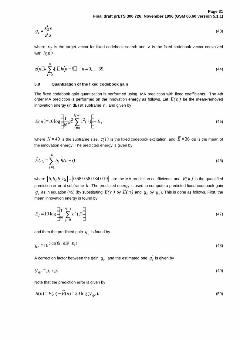
gc
t
t= x z
z z2 (43)
where x2 is the target vector for fixed codebook search and z is the fixed codebook vector convolved
with h n( ) ,
( ) ( ) ( )z n c i h n i ni
n
= − ==∑
0
0 39, , , .� (44)
5.8 Quantization of the fixed codebook gain
The fixed codebook gain quantization is performed using MA prediction with fixed coefficients. The 4thorder MA prediction is performed on the innovation energy as follows. Let E n( ) be the mean-removed
innovation energy (in dB) at subframe n , and given by
E nN
g c i Eci
N
( ) ( ) ,=
−
=
−
∑101 2 2
0
1
log (45)
where N =40 is the subframe size, c i( ) is the fixed codebook excitation, and E =36 dB is the mean of
the innovation energy. The predicted energy is given by
~( ) � ( )E n b R n ii
i
= −=∑
1
4
, (46)
where [ ] [ ]b b b b1 2 3 4 0 68 0 58 0 34 019= . . . . are the MA prediction coefficients, and �( )R k is the quantified
prediction error at subframe k . The predicted energy is used to compute a predicted fixed-codebook gain
gc' as in equation (45) (by substituting E n( ) by
~( )E n and gc by gc
' ). This is done as follows. First, the
mean innovation energy is found by
EN
c jIj
N
=
=
−
∑101 2
0
1
log ( ) (47)
and then the predicted gain gc' is found by
gcE n E EI' . (~
( ) ).= + −100 05(48)
A correction factor between the gain gc and the estimated one gc' is given by
γ gc c cg g= / ' . (49)
Note that the prediction error is given by
R n E n E n gc( ) ( )~( ) ( ).= − = 20 log γ (50)

Page 32Final draft prETS 300 726: November 1996 (GSM 06.60 version 5.1.1)
The correction factor γ gc is quantified using a 5-bit codebook. The quantization table search is performed
by minimizing the error
E g gQ c gc c= −( � ) .'γ 2 (51)
Once the optimum value �γ gc is chosen, the quantified fixed codebook gain is given by � � 'g gc gc c=γ .
5.9 Memory update
An update of the states of the synthesis and weighting filters is needed in order to compute the targetsignal in the next subframe.
After the two gains are quantified, the excitation signal, u n( ) , in the present subframe is found by
u n g v n g c n np c( ) � ( ) � ( ), , , ,= + =0 39� (52)
where �gp and �gc are the quantified adaptive and fixed codebook gains, respectively, v n( ) the adaptive
codebook vector (interpolated past excitation), and c n( ) is the fixed codebook vector (algebraic code
including pitch sharpening). The states of the filters can be updated by filtering the signal res n u nLP( ) ( )−(difference between residual and excitation) through the filters 1 �( )A z and A z A z( / ) ( / )γ γ1 2 for the
40-sample subframe and saving the states of the filters. This would require 3 filterings. A simplerapproach which requires only one filtering is as follows. The local synthesized speech, �( )s n , is computed
by filtering the excitation signal through 1 �( )A z . The output of the filter due to the input res n u nLP( ) ( )−is equivalent to e n s n s n( ) ( ) �( )= − . So the states of the synthesis filter 1 �( )A z are given by
e n n( ), , ,=30 39� . Updating the states of the filter A z A z( / ) ( / )γ γ1 2 can be done by filtering the
error signal e n( ) through this filter to find the perceptually weighted error e nw( ) . However, the signal
e nw( ) can be equivalently found by
e n x n g y n g z nw p c( ) ( ) � ( ) � ( ).= − − (53)
Since the signals x n y n( ), ( ) , and z n( ) are available, the states of the weighting filter are updated by
computing e nw( ) as in equation (53) for n = 30 39, ,� . This saves two filterings.
6 Functional description of the decoder
The function of the decoder consists of decoding the transmitted parameters (LP parameters, adaptivecodebook vector, adaptive codebook gain, fixed codebook vector, fixed codebook gain) and performingsynthesis to obtain the reconstructed speech. The reconstructed speech is then post-filtered andupscaled. The signal flow at the decoder is shown in figure 4.
6.1 Decoding and speech synthesis
The decoding process is performed in the following order:
Decoding of LP filter parameters: The received indices of LSP quantization are used to reconstruct thetwo quantified LSP vectors. The interpolation described in section 5.2.6 is performed to obtain 4interpolated LSP vectors (corresponding to 4 subframes). For each subframe, the interpolated LSP vectoris converted to LP filter coefficient domain ak , which is used for synthesizing the reconstructed speech in
the subframe.

Page 33Final draft prETS 300 726: November 1996 (GSM 06.60 version 5.1.1)
The following steps are repeated for each subframe:
1) Decoding of the adaptive codebook vector: The received pitch index (adaptive codebook index)is used to find the integer and fractional parts of the pitch lag. The adaptive codebook vector v n( )is found by interpolating the past excitation u n( ) (at the pitch delay) using the FIR filter described insection 5.6.
2) Decoding of the adaptive codebook gain: The received index is used to readily find thequantified adaptive codebook gain, �gp from the quantization table.
3) Decoding of the innovative codebook vector: The received algebraic codebook index is used toextract the positions and amplitudes (signs) of the excitation pulses and to find the algebraiccodevector c n( ) . If the integer part of the pitch lag is less than the subframe size 40, the pitch
sharpening procedure is applied which translates into modifying c n( ) byc n c n c n T( ) ( ) ( )= + −β ,
where β is the decoded pitch gain, �gp , bounded by [0.0,1.0].
4) Decoding of the fixed codebook gain: The received index gives the fixed codebook gaincorrection factor �γ gc . The estimated fixed codebook gain ′gc is found as described in section 5.7.
First, the predicted energy is found by
~( ) � ( )E n b R n ii
i
= −=∑
1
4
(54)
and then the mean innovation energy is found by
EN
c jIj
N
=
=
−
∑101 2
0
1
log ( ) (55)
The predicted gain ′gc is found by
gcE n E EI' . (~
( ) ).= + −100 05. (56)
The quantified fixed codebook gain is given by
� � 'g gc gc c=γ (57)
5) Computing the reconstructed speech: The excitation at the input of the synthesis filter is givenby
u n g v n g c np c( ) � ( ) � ( )= + (58)
Before the speech synthesis, a post-processing of excitation elements is performed. This meansthat the total excitation is modified by emphasizing the contribution of the adaptive codebook vector:
�( )( ) . � ( ), � .
( ), � .u n
u n g v n g
u n gp p
p=
+ >≤
0 25 0 5
0 5
β(59)
Adaptive gain control (AGC) is used to compensate for the gain difference between the non-emphasized excitation ( )u n and emphasized excitation ( )�u n The gain scaling factor η for theemphasized excitation is computed by:

Page 34Final draft prETS 300 726: November 1996 (GSM 06.60 version 5.1.1)
η =
>
≤
=
=
∑∑
u n
u n
g
g
n
n
p
p
20
39
20
39
0 5
10 0 5
( )
� ( ),
� .
. � .
(60)
The gain-scaled emphasized excitation signal � ' ( )u n is given by
�' ( ) �( )u n u n= η (61)
The reconstructed speech for the subframe of size 40 is given by
�( ) �' ( ) � �( ), , , .s n u n a s n i nii
= − − ==∑
1
10
0 39 � (62)
where �ai are the interpolated LP filter coefficients.
The synthesized speech �( )s n is then passed through an adaptive postfilter which is described in the
following section.
6.2 Post-processing
Post-processing consists of two functions: adaptive post-filtering and signal up-scaling.
6.2.1 Adaptive post-filtering
The adaptive postfilter is the cascade of two filters: a formant postfilter, and a tilt compensation filter. Thepostfilter is updated every subframe of 5 ms.
The formant postfilter is given by
H zA z
A zf
n
d( )
� ( / )� ( / )
= γγ
(63)
where � ( )A z is the received quantified (and interpolated) LP inverse filter (LP analysis is not performed at
the decoder), and the factors γ n and γ d control the amount of the formant post-filtering.
Finally, the filter H zt ( ) compensates for the tilt in the formant postfilter H zf ( ) and is given by
H z zt ( ) ( )= − −1 1µ (64)
where µ γ= tk1' is a tilt factor, with k1' being the first reflection coefficient calculated on the truncated
( )Lh = 22 impulse response, h nf ( ) , of the filter � ( / ) / � ( / )A z A zn dγ γ . k1' is given by
kr
rr i h j h j ih
hh f f
j
L ih
10
11
0'
( )
( ); ( ) ( ) ( )= = +
=
− −
∑ (65)

Page 35Final draft prETS 300 726: November 1996 (GSM 06.60 version 5.1.1)
The post-filtering process is performed as follows. First, the synthesized speech �( )s n is inverse filtered
through � ( / )A z nγ to produce the residual signal �( )r n . The signal �( )r n is filtered by the synthesis filter
1/ � ( / )A z dγ . Finally, the signal at the output of the synthesis filter 1/ � ( / )A z dγ is passed to the tilt
compensation filter h zt ( ) resulting in the post-filtered speech signal � ( )s nf .
Adaptive gain control (AGC) is used to compensate for the gain difference between the synthesizedspeech signal �( )s n and the post-filtered signal � ( )s nf . The gain scaling factor γ sc for the present
subframe is computed by
γ scn
fn
s n
s n
= =
=
∑
∑
� ( )
� ( )
2
0
39
2
0
39 (66)
The gain-scaled post-filtered signal � ( )′s n is given by
� ( ) ( )� ( )′ =s n n s nsc fβ (67)
where β sc n( ) is updated in sample-by-sample basis and given by
β αβ α γsc sc scn n( ) ( ) ( )= − + −1 1 (68)
where α is a AGC factor with value of 0.9.
The adaptive post-filtering factors are given by: γ n = 0 7. , γ d = 0 75. and
γ tk
otherwise=
>
0 8 0
01. , '
,. (69)
6.2.2 Up-scaling
Up-scaling consists of multiplying the post-filtered speech by a factor of 2 to compensate for the down-scaling by 2 which is applied to the input signal.
7 Variables, constants and tables in the C-code of the GSM EFR codec
The various components of the 12,2 kbit/s GSM enhanced full rate codec are described in the form of afixed-point bit-exact ANSI C code, which is found in GSM 06.53 [6]. This C simulation is an integratedsoftware of the speech codec, VAD/DTX, comfort noise and bad frame handler functions. In the fixed-point ANSI C simulation, all the computations are performed using a predefined set of basic operators.
Two types of variables are used in the fixed-point implementation. These two types are signed integers in2's complement representation, defined by:
Word16 16 bit variables
Word32 32 bit variables
The variables of the Word16 type are denoted var1, var2, ..., varn, and those of type Word32 are denotedL_var1, L_var2, ..., L_varn.
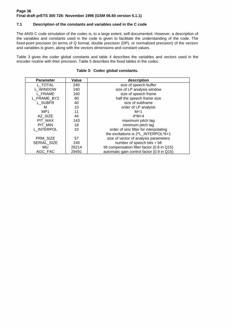
Page 36Final draft prETS 300 726: November 1996 (GSM 06.60 version 5.1.1)
7.1 Description of the constants and variables used in the C code
The ANSI C code simulation of the codec is, to a large extent, self-documented. However, a description ofthe variables and constants used in the code is given to facilitate the understanding of the code. Thefixed-point precision (in terms of Q format, double precision (DP), or normalized precision) of the vectorsand variables is given, along with the vectors dimensions and constant values.
Table 3 gives the coder global constants and table 4 describes the variables and vectors used in theencoder routine with their precision. Table 5 describes the fixed tables in the codec.
Table 3: Codec global constants.
Parameter Value descriptionL_TOTAL 240 size of speech buffer
L_WINDOW 240 size of LP analysis windowL_FRAME 160 size of speech frame
L_FRAME_BY2 80 half the speech frame sizeL_SUBFR 40 size of subframe
M 10 order of LP analysisMP1 11 M+1
AZ_SIZE 44 4*M+4PIT_MAX 143 maximum pitch lagPIT_MIN 18 minimum pitch lag
L_INTERPOL 10 order of sinc filter for interpolatingthe excitations is 2*L_INTERPOL*6+1
PRM_SIZE 57 size of vector of analysis parametersSERIAL_SIZE 245 number of speech bits + bfi
MU 26214 tilt compensation filter factor (0.8 in Q15)AGC_FAC 29491 automatic gain control factor (0.9 in Q15)

Page 37Final draft prETS 300 726: November 1996 (GSM 06.60 version 5.1.1)
Table 4: Description of the coder vectors and variables
Parameter size precision descriptionspeech -80..159 Q0 speech buffer
wsp -143..159 Q0 weighted speech bufferexc -(143+11)..159 Q0 LP excitation
F_gamma1 0..9 Q15 spectral expansion factorsF_gamma2 0..9 Q15 spectral expansion factors
lsp_old 0..9 Q15 LSP vector in past framelsp_old_q 0..9 Q15 quantified LSP vector in past framemem_syn 0..9 Q0 memory of synthesis filtermem_w 0..9 Q0 memory of weighting filter (applied to input)
mem_wO 0..9 Q0 memory of weighting filter (applied to error)error -10..39 Q0 error signal (input minus synthesized speech)
r_1 & r_h 0..10 normalized DP correlations of windowed speech (low and hi)A_t 11x4 Q12 LP filter coefficients in 4 subframesAq_t 11x4 Q12 quantified LP filter coefficients in
4 subframesAp1 0..10 Q12 LP coefficients with spectral expansionAp2 0..10 Q12 LP coefficients with spectral expansion
lsp_new 0..9 Q15 LSP vector in 4th subframelsp_new_q 0..9 Q15 quantified LSP vector in 4th subframe
lsp_mid 0..9 Q15 LSP vector in 2nd subframelsp_mid_q 0..9 Q15 quantified LSP vector in 2nd subframe
code 0..39 Q12 fixed codebook excitation vectorh1 0..39 Q12 impulse response of weighted synthesis filterxn 0..39 Q0 target vector in pitch searchxn2 0..39 Q0 target vector in algebraic codebook searchdn 0..39 scaled max
< 8192backward filtered target vector
y1 0..39 Q0 filtered adaptive codebook vectory2 0..39 Q12 filtered fixed codebook vector
zero 0..39 zero vectorres2 0..39 long-term prediction residual
gain_pit scalar Q12 adaptive codebook gaingain_code scalar Q0 algebraic codebook gain
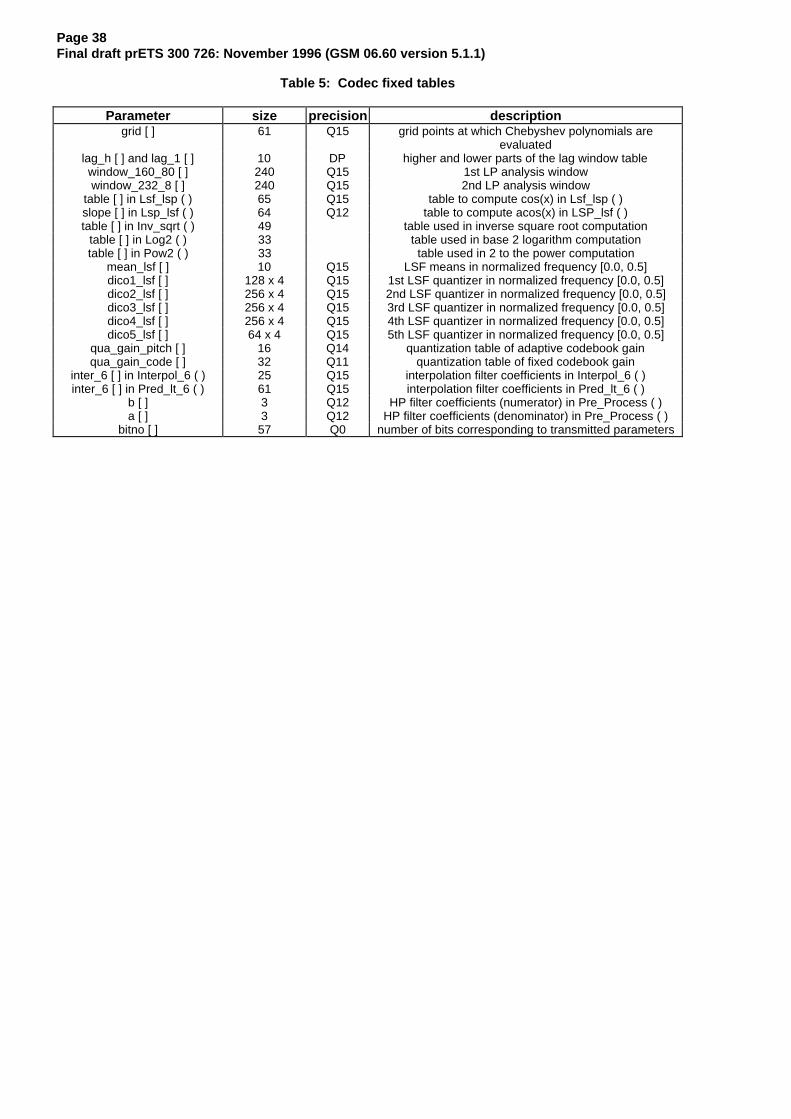
Page 38Final draft prETS 300 726: November 1996 (GSM 06.60 version 5.1.1)
Table 5: Codec fixed tables
Parameter size precision descriptiongrid [ ] 61 Q15 grid points at which Chebyshev polynomials are
evaluatedlag_h [ ] and lag_1 [ ] 10 DP higher and lower parts of the lag window tablewindow_160_80 [ ] 240 Q15 1st LP analysis windowwindow_232_8 [ ] 240 Q15 2nd LP analysis window
table [ ] in Lsf_lsp ( ) 65 Q15 table to compute cos(x) in Lsf_lsp ( )slope [ ] in Lsp_lsf ( ) 64 Q12 table to compute acos(x) in LSP_lsf ( )table [ ] in Inv_sqrt ( ) 49 table used in inverse square root computation
table [ ] in Log2 ( ) 33 table used in base 2 logarithm computationtable [ ] in Pow2 ( ) 33 table used in 2 to the power computation
mean_lsf [ ] 10 Q15 LSF means in normalized frequency [0.0, 0.5]dico1_lsf [ ] 128 x 4 Q15 1st LSF quantizer in normalized frequency [0.0, 0.5]dico2_lsf [ ] 256 x 4 Q15 2nd LSF quantizer in normalized frequency [0.0, 0.5]dico3_lsf [ ] 256 x 4 Q15 3rd LSF quantizer in normalized frequency [0.0, 0.5]dico4_lsf [ ] 256 x 4 Q15 4th LSF quantizer in normalized frequency [0.0, 0.5]dico5_lsf [ ] 64 x 4 Q15 5th LSF quantizer in normalized frequency [0.0, 0.5]
qua_gain_pitch [ ] 16 Q14 quantization table of adaptive codebook gainqua_gain_code [ ] 32 Q11 quantization table of fixed codebook gain
inter_6 [ ] in Interpol_6 ( ) 25 Q15 interpolation filter coefficients in Interpol_6 ( )inter_6 [ ] in Pred_lt_6 ( ) 61 Q15 interpolation filter coefficients in Pred_lt_6 ( )
b [ ] 3 Q12 HP filter coefficients (numerator) in Pre_Process ( )a [ ] 3 Q12 HP filter coefficients (denominator) in Pre_Process ( )
bitno [ ] 57 Q0 number of bits corresponding to transmitted parameters

Page 39Final draft prETS 300 726: November 1996 (GSM 06.60 version 5.1.1)
Table 6: Source Encoder output parameters in order of occurrence and bit allocation within thespeech frame of 244 bits/20 ms
Bits (MSB-LSB) Descriptions1 - s7 index of 1st LSF submatrixs8 - s15 index of 2nd LSF submatrixs16 - s23 index of 3rd LSF submatrix
s24 sign of 3rd LSF submatrixs25 - s32 index of 4th LSF submatrixs33 - s38 index of 5th LSF submatrix
subframe 1s39 - s47 adaptive codebook indexs48 - s51 adaptive codebook gain
s52 sign information for 1st and 6th pulsess53 - s55 position of 1st pulse
s56 sign information for 2nd and 7th pulsess57 - s59 position of 2nd pulse
s60 sign information for 3rd and 8th pulsess61 - s63 position of 3rd pulse
s64 sign information for 4th and 9th pulsess65 - s67 position of 4th pulse
s68 sign information for 5th and 10th pulsess69 - s71 position of 5th pulses72 - s74 position of 6th pulses75 - s77 position of 7th pulses78 - s80 position of 8th pulses81 - s83 position of 9th pulses84 - s86 position of 10th pulses87 - s91 fixed codebook gain
subframe 2s92 - s97 adaptive codebook index (relative)s98 - s141 same description as s48 - s91
subframe 3s142 - s194 same description as s39 - s91
subframe 4s195 - s244 same description as s92 - s141

Page 40Final draft prETS 300 726: November 1996 (GSM 06.60 version 5.1.1)
8 Homing sequences
8.1 Functional description
The enhanced full rate speech codec is described in a bit-exact arithmetic to allow for easy type approvalas well as general testing purposes of the enhanced full rate speech codec.
The response of the codec to a predefined input sequence can only be foreseen if the internal statevariables of the codec are in a predefined state at the beginning of the experiment. Therefore, the codechas to be put in a so called home state before a bit-exact test can be performed. This is usually done by areset (a procedure in which the internal state variables of the codec are set to their defined initial values).
To allow a reset of the codec in remote locations, special homing frames have been defined for theencoder and the decoder, thus enabling a codec homing by inband signalling.
The codec homing procedure is defined in such a way, that in either direction (encoder or decoder) thehoming functions are called after processing the homing frame that is input. The output corresponding tothe first homing frame is therefore dependent on the codec state when receiving that frame and henceusually not known. The response to any further homing frame in one direction is by definition a homingframe of the other direction. This procedure allows homing of both, the encoder and decoder from eitherside, if a loop back configuration is implemented, taking proper framing into account.
8.2 Definitions
Encoder homing frame: The encoder homing frame consists of 160 identical samples, each 13 bits long,with the least significant bit set to "one" and all other bits set to "zero". When written to 16-bit words withleft justification, the samples have a value of 0008 hex. The speech decoder has to produce this frame asa response to the second and any further decoder homing frame if at least two decoder homing frameswere input to the decoder consecutively.
Decoder homing frame: The decoder homing frame has a fixed set of speech parameters as describedin table7. It is the natural response of the speech encoder to the second and any further encoder homingframe if at least two encoder homing frames were input to the encoder consecutively.
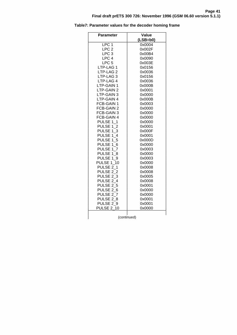
Page 41Final draft prETS 300 726: November 1996 (GSM 06.60 version 5.1.1)
Table7: Parameter values for the decoder homing frame
Parameter Value(LSB=b0)
LPC 1 0x0004LPC 2 0x002FLPC 3 0x00B4LPC 4 0x0090LPC 5 0x003E
LTP-LAG 1 0x0156LTP-LAG 2 0x0036LTP-LAG 3 0x0156LTP-LAG 4 0x0036LTP-GAIN 1 0x000BLTP-GAIN 2 0x0001LTP-GAIN 3 0x0000LTP-GAIN 4 0x000BFCB-GAIN 1 0x0003FCB-GAIN 2 0x0000FCB-GAIN 3 0x0000FCB-GAIN 4 0x0000PULSE 1_1 0x0000PULSE 1_2 0x0001PULSE 1_3 0x000FPULSE 1_4 0x0001PULSE 1_5 0x000DPULSE 1_6 0x0000PULSE 1_7 0x0003PULSE 1_8 0x0000PULSE 1_9 0x0003PULSE 1_10 0x0000PULSE 2_1 0x0008PULSE 2_2 0x0008PULSE 2_3 0x0005PULSE 2_4 0x0008PULSE 2_5 0x0001PULSE 2_6 0x0000PULSE 2_7 0x0000PULSE 2_8 0x0001PULSE 2_9 0x0001PULSE 2_10 0x0000
(continued)

Page 42Final draft prETS 300 726: November 1996 (GSM 06.60 version 5.1.1)
Table 7 (concluded): Parameter values for the decoder homing frame
Parameter Value(LSB=b0)
PULSE 3_1 0x0000PULSE 3_2 0x0000PULSE 3_3 0x0000PULSE 3_4 0x0000PULSE 3_5 0x0000PULSE 3_6 0x0000PULSE 3_7 0x0000PULSE 3_8 0x0000PULSE 3_9 0x0000PULSE 3_10 0x0000PULSE 4_1 0x0000PULSE 4_2 0x0000PULSE 4_3 0x0000PULSE 4_4 0x0000PULSE 4_5 0x0000PULSE 4_6 0x0000PULSE 4_7 0x0000PULSE 4_8 0x0000PULSE 4_9 0x0000PULSE 4_10 0x0000
8.3 Encoder homing
Whenever the enhanced full rate speech encoder receives at its input an encoder homing frame exactlyaligned with its internal speech frame segmentation, the following events take place:
Step 1: The speech encoder performs its normal operation including VAD and DTX andproduces a speech parameter frame at its output which is in general unknown.But if the speech encoder was in its home state at the beginning of that frame,then the resulting speech parameter frame is identical to the decoder homingframe (this is the way how the decoder homing frame was constructed).
Step 2: After successful termination of that operation the speech encoder provokes thehoming functions for all sub-modules including VAD and DTX and sets all statevariables into their home state. On the reception of the next input frame, thespeech encoder will start from its home state.
NOTE: Applying a sequence of N encoder homing frames will cause at least N-1 decoderhoming frames at the output of the speech encoder.
8.4 Decoder homing
Whenever the speech decoder receives at its input a decoder homing frame, then the following eventstake place:
Step 1: The speech decoder performs its normal operation and produces a speechframe at its output which is in general unknown. But if the speech decoder wasin its home state at the beginning of that frame, then the resulting speech frameis replaced by the encoder homing frame. This would not naturally be the casebut is forced by this definition here.
Step 2: After successful termination of that operation the speech decoder provokes thehoming functions for all sub-modules including the comfort noise generator andsets all state variables into their home state. On the reception of the next inputframe, the speech decoder will start from its home state.
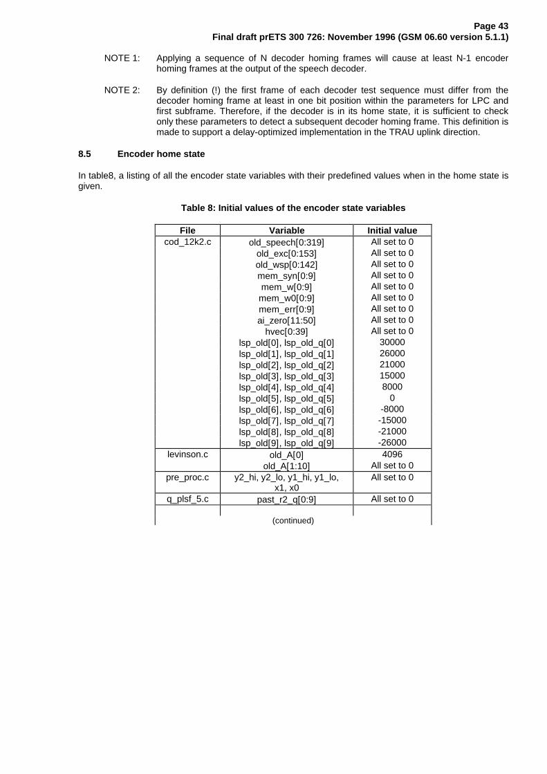
Page 43Final draft prETS 300 726: November 1996 (GSM 06.60 version 5.1.1)
NOTE 1: Applying a sequence of N decoder homing frames will cause at least N-1 encoderhoming frames at the output of the speech decoder.
NOTE 2: By definition (!) the first frame of each decoder test sequence must differ from thedecoder homing frame at least in one bit position within the parameters for LPC andfirst subframe. Therefore, if the decoder is in its home state, it is sufficient to checkonly these parameters to detect a subsequent decoder homing frame. This definition ismade to support a delay-optimized implementation in the TRAU uplink direction.
8.5 Encoder home state
In table8, a listing of all the encoder state variables with their predefined values when in the home state isgiven.
Table 8: Initial values of the encoder state variables
File Variable Initial valuecod_12k2.c old_speech[0:319] All set to 0
old_exc[0:153] All set to 0old_wsp[0:142] All set to 0mem_syn[0:9] All set to 0mem_w[0:9] All set to 0mem_w0[0:9] All set to 0mem_err[0:9] All set to 0ai_zero[11:50] All set to 0
hvec[0:39] All set to 0lsp_old[0], lsp_old_q[0] 30000lsp_old[1], lsp_old_q[1] 26000lsp_old[2], lsp_old_q[2] 21000lsp_old[3], lsp_old_q[3] 15000lsp_old[4], lsp_old_q[4] 8000lsp_old[5], lsp_old_q[5] 0lsp_old[6], lsp_old_q[6] -8000lsp_old[7], lsp_old_q[7] -15000lsp_old[8], lsp_old_q[8] -21000lsp_old[9], lsp_old_q[9] -26000
levinson.c old_A[0] 4096old_A[1:10] All set to 0
pre_proc.c y2_hi, y2_lo, y1_hi, y1_lo,x1, x0
All set to 0
q_plsf_5.c past_r2_q[0:9] All set to 0
(continued)

Page 44Final draft prETS 300 726: November 1996 (GSM 06.60 version 5.1.1)
Table 8 (concluded): Initial values of the encoder state variables
File Variable Initial valueq_gains.c past_qua_en[0:3] All set to -2381
pred[0] 44pred[1] 37pred[2] 22pred[3] 12
dtx.c txdtx_hangover 7txdtx_N_elapsed 0x7fff
txdtx_ctrl 0x0003old_CN_mem_tx[0:5] All set to 0
lsf_old_tx[0:6][0] 1384lsf_old_tx[0:6][1] 2077lsf_old_tx[0:6][2] 3420lsf_old_tx[0:6][3] 5108lsf_old_tx[0:6][4] 6742lsf_old_tx[0:6][5] 8122lsf_old_tx[0:6][6] 9863lsf_old_tx[0:6][7] 11092lsf_old_tx[0:6][8] 12714lsf_old_tx[0:6][9] 13701
gain_code_old_tx[0:27] All set to 0L_pn_seed_tx 0x70816958
buf_p_tx 0
Initial values for variables used by the VAD algorithm are listed in GSM 06.32 [4].
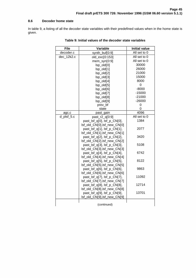
Page 45Final draft prETS 300 726: November 1996 (GSM 06.60 version 5.1.1)
8.6 Decoder home state
In table 9, a listing of all the decoder state variables with their predefined values when in the home state isgiven.
Table 9: Initial values of the decoder state variables
File Variable Initial valuedecoder.c synth_buf[0:9] All set to 0
dec_12k2.c old_exc[0:153] All set to 0mem_syn[0:9] All set to 0
lsp_old[0] 30000lsp_old[1] 26000lsp_old[2] 21000lsp_old[3] 15000lsp_old[4] 8000lsp_old[5] 0lsp_old[6] -8000lsp_old[7] -15000lsp_old[8] -21000lsp_old[9] -26000prev_bf 0
state 0agc.c past_gain 4096
d_plsf_5.c past_r2_q[0:9] All set to 0past_lsf_q[0], lsf_p_CN[0],
lsf_old_CN[0],lsf_new_CN[0]1384
past_lsf_q[1], lsf_p_CN[1],lsf_old_CN[1],lsf_new_CN[1]
2077
past_lsf_q[2], lsf_p_CN[2],lsf_old_CN[2],lsf_new_CN[2]
3420
past_lsf_q[3], lsf_p_CN[3],lsf_old_CN[3],lsf_new_CN[3]
5108
past_lsf_q[4], lsf_p_CN[4],lsf_old_CN[4],lsf_new_CN[4]
6742
past_lsf_q[5], lsf_p_CN[5],lsf_old_CN[5],lsf_new_CN[5]
8122
past_lsf_q[6], lsf_p_CN[6],lsf_old_CN[6],lsf_new_CN[6]
9863
past_lsf_q[7], lsf_p_CN[7],lsf_old_CN[7],lsf_new_CN[7]
11092
past_lsf_q[8], lsf_p_CN[8],lsf_old_CN[8],lsf_new_CN[8]
12714
past_lsf_q[9], lsf_p_CN[9],lsf_old_CN[9],lsf_new_CN[9]
13701
(continued)

Page 46Final draft prETS 300 726: November 1996 (GSM 06.60 version 5.1.1)
Table 9 (concluded): Initial values of the decoder state variables
File Variable Initial valued_gains.c pbuf[0:4] All set to 410
gbuf[0:4] All set to 1past_gain_pit 0
past_gain_code 0prev_gp 4096prev_gc 1
gcode0_CN 0gain_code_old_CN 0gain_code_new_CN 0
gain_code_muting_CN 0past_qua_en[0:3] All set to -2381
pred[0] 44pred[1] 37pred[2] 22pred[3] 12
dtx.c rxdtx_aver_period 7rxdtx_N_elapsed 0x7fff
rxdtx_ctrl 0x0001lsf_old_rx[0:6][0] 1384lsf_old_rx[0:6][1] 2077lsf_old_rx[0:6][2] 3420lsf_old_rx[0:6][3] 5108lsf_old_rx[0:6][4] 6742lsf_old_rx[0:6][5] 8122lsf_old_rx[0:6][6] 9863lsf_old_rx[0:6][7] 11092lsf_old_rx[0:6][8] 12714lsf_old_rx[0:6][9] 13701
gain_code_old_rx[0:27] All set to 0L_pn_seed_rx 0x70816958rx_dtx_state 23
prev_SID_frames_lost 0buf_p_rx 0
dec_lag6.c old_T0 40preemph.c mem_pre 0pstfilt2.c mem_syn_pst[0:9] All set to 0
res2[0:39] All set to 0
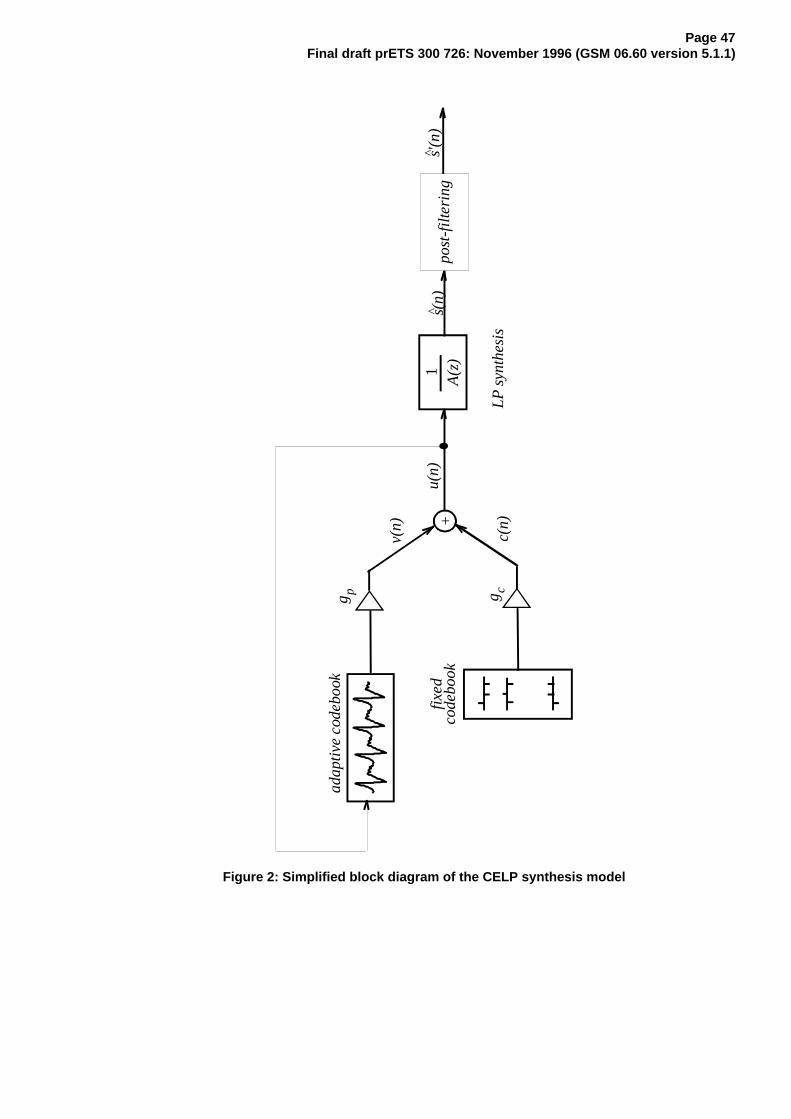
Page 47Final draft prETS 300 726: November 1996 (GSM 06.60 version 5.1.1)
A(z
)1
s(n
)^
+
v(n)
c(n)
u(n
)
g c
fixe
dco
debook
adaptiv
e c
ode
book
g p
LP
syn
the
sis
po
st-f
ilte
ring
s'(n
)^
Figure 2: Simplified block diagram of the CELP synthesis model

Page 48Final draft prETS 300 726: November 1996 (GSM 06.60 version 5.1.1)
win
dow
ing
and
au
toco
rrel
atio
nR
[ ]
Levi
nson
-D
urb
inR
[ ]A
(z)
A(z
) LS
Pqu
antiz
atio
n
com
pute
targ
etfo
rin
nova
tion
upd
ate
filte
rm
emor
ies
for
next
sub
fram
e
Op
en
-lo
op
pitc
h s
ea
rch
Ada
ptiv
e co
debo
okse
arch
Inno
vativ
e co
debo
okse
arch
Filt
er m
emor
yup
date
inte
rpol
atio
n
subf
ram
esL
SP
A(z
)
LS
P
com
pute
wei
ght
edsp
eech
(4 s
ub
fram
es)
find
op
en-l
oo
p p
itch
find
bes
t in
nova
tion
fixed
co
debo
okga
in
quan
tizat
ion
A(z
)^
x(n)
pitc
hin
dex
code
ind
ex
fram
esu
bfra
me
s(n)
com
pute
targ
etfo
r ad
aptiv
eco
debo
ok
To
find
best
del
ayan
d ga
in
x(n) co
mpu
teim
puls
ere
spon
se
A(z
)^A(z
)h(
n)
h(n)
A(z
)
LPC
ana
lysi
s(t
wic
e pe
r fr
ame)
A(z
)
(tw
ice
per
fram
e)
x (n
)2
quan
tize
LTP
-gai
n
com
pute
adap
tive
code
book
cont
ribut
ion
LSP
indi
ces
LTP
gai
nin
dex
gai
n in
dex
fixed
cod
eboo
k
inte
rpol
atio
nfo
r th
e 4
sub
fram
esL
SP
A(z
)^
for
the
4
Pre
-pro
cess
ing
Pre
-pro
cess
ing
com
pute
exci
tatio
n
Figure 3: Simplified block diagram of the GSM enhanced full rate encoder
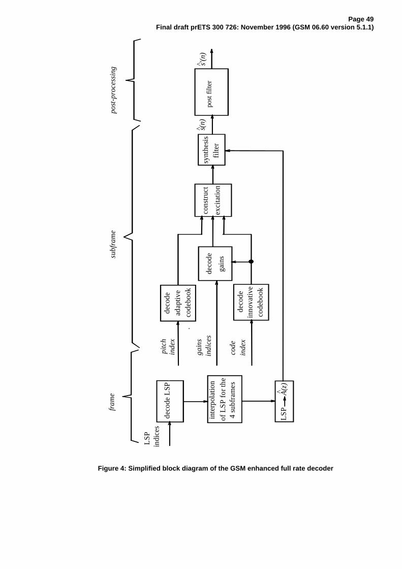
Page 49Final draft prETS 300 726: November 1996 (GSM 06.60 version 5.1.1)
LS
Pin
dice
s
dec
ode
LS
P
inte
rpol
atio
n
of L
SP
for
the
4 s
ubf
ram
es
LSP
deco
dead
aptiv
eco
debo
ok
deco
dein
nova
tive
code
book
pitc
hin
dex
cod
ein
dex
deco
de
gain
s
A(z
)^
cons
truc
t
exci
tatio
n
fra
me
subf
ram
epo
st-p
roce
ssin
g s'(n
)^
s(n)
^po
st fi
lter
gai
ns
ind
ices
synt
hesi
sfil
ter
Figure 4: Simplified block diagram of the GSM enhanced full rate decoder
Page 50Final draft prETS 300 726: November 1996 (GSM 06.60 version 5.1.1)
9 Bibliography
1) M.R. Schroeder and B.S. Atal, "Code-Excited Linear Prediction (CELP): Highquality speech at very low bit rates,"' Proc. ICASSP'85, pp. 937-940, 1985.
2) Y. Tohkura and F. Itakura, "Spectral smoothing technique in PARCOR speechanalysis-synthesis," IEEE Trans. on ASSP, vol. 26, no. 6, pp. 587-596, Dec.1978.
3) L.R. Rabiner and R.W. Schaefer. Digital processing of speech signals. Prentice-Hall Int., 1978.
4) F. Itakura, "Line spectral representation of linear predictive coefficients ofspeech signals," J. Acoust. Soc. Amer, vol. 57, Supplement no. 1, S35, 1975.
5) F.K. Soong and B.H. Juang, "Line spectrum pair (LSP) and speech datacompression", Proc. ICASSP'84, pp. 1.10.1-1.10.4, 1984.
6) P. Kabal and R.P. Ramachandran, "The computation of line spectralfrequencies using Chebyshev polynomials", IEEE Trans. on ASSP, vol. 34, no.6, pp. 1419-1426, Dec. 1986.
7) C. Laflamme, J-P. Adoul, R. Salami, S. Morissette, and P. Mabilleau, "16 kpbswideband speech coding technique based on algebraic CELP" Proc.ICASSP'91, pp. 13-16.

Page 51Final draft prETS 300 726: November 1996 (GSM 06.60 version 5.1.1)
History
Document history
March 1996 Public Enquiry PE 103: 1996-03-04 to 1996-06-28
November 1996 Vote V 115: 1996-11-25 to 1997-01-17