ex-post economic evaluation of - bitre.gov.au · ex-post economic evaluation of ... vi ex-post...

Road

R E S E A R C H R E P O R T 1 4 5

bitreEx-post Economic Evaluation of National Road Investment Projects

Volume 2 Case Studies

Bureau of Infrastructure, Transport and Regional Economics

Ex-post Economic Evaluation of National Road Investment Projects

Report 145

Volume 2 Case Studies

Department of Infrastructure, Regional Development and Cities Canberra, Australia

© Commonwealth of Australia 2018

ISSN: 1440-9569 ISBN: 978-1-925531-66-4 January 2018/INFRA3312

Ownership of intellectual property rights in this publication

Unless otherwise noted, copyright (and any other intellectual property rights, if any) in this publication is owned by the Commonwealth of Australia (referred to below as the Commonwealth).

Disclaimer

The material contained in this publication is made available on the understanding that the Commonwealth is not providing professional advice, and that users exercise their own skill and care with respect to its use, and seek independent advice if necessary.

The Commonwealth makes no representations or warranties as to the contents or accuracy of the information contained in this publication. To the extent permitted by law, the Commonwealth disclaims liability to any person or organisation in respect of anything done, or omitted to be done, in reliance upon information contained in this publication.

Creative Commons licence

With the exception of (a) the Coat of Arms; and (b) the Department of Infrastructure, Regional Development and Cities photos and graphics, copyright in this publication is licensed under a Creative Commons Attribution 3.0 Australia Licence.

Creative Commons Attribution 3.0 Australia Licence is a standard form licence agreement that allows you to copy, communicate and adapt this publication provided that you attribute the work to the Commonwealth and abide by the other licence terms. A summary of the licence terms is available from http://creativecommons.org/licenses/by/3.0/au/deed.en. The full licence terms are available from http://creativecommons.org/licenses/by/3.0/au/legalcode.

Use of the Coat of Arms

The Department of the Prime Minister and Cabinet sets the terms under which the Coat of Arms is used. Please refer to the Department’s Commonwealth Coat of Arms and Government Branding web page in particular, the Commonwealth Coat of Arms Information and Guidelines publication.

An appropriate citation for this report is:

Bureau of Infrastructure, Transport and Regional Economics (BITRE), 2018, Ex-post Economic Evaluation of National Road Investment Projects – Volume 2 Case Studies, Report 145, BITRE, Canberra ACT.

Contact usThis publication is available in PDF format. All other rights are reserved, including in relation to any Departmental logos or trade marks which may exist. For enquiries regarding the licence and any use of this publication, please contact:Bureau of Infrastructure, Transport and Regional Economics (BITRE) Department of Infrastructure, Regional Development and Cities GPO Box 501, Canberra ACT 2601, AustraliaTelephone: (international) +61 2 6274 7210 Fax: (international) +61 2 6274 6855 Email: [email protected] Website: www.bitre.gov.au

• v •

Contents

Appendix B.1 Bruce Highway Upgrade – Cooroy to Curra Section B ............................................... 1

Appendix B.2 Dampier Highway Upgrade – Broadhurst Road to Burrup Peninsular Road ...................................................................................................................................39

Appendix B.3 Bulahdelah Bypass ..............................................................................................................................85

Appendix B.4 Nagambie Bypass .............................................................................................................................133

Appendix B.5 Northern Expressway ..................................................................................................................179


Ex-post Economic Evaluation:

Bruce Highway Upgrade – Cooroy to Curra Section B

Appendix B.1


• 3 •

Contents

Summary ........................................................................................................................................................................ 9

I Introduction .................................................................................................................................................................11

II Description of Cooroy to Curra Section B upgrade project ......................................................13

III Review of ex-ante CBA .......................................................................................................................................15

IV Methodological issues in ex-post evaluation ..........................................................................................17

Treatment of Queensland Water Infrastructure (QWI) contribution .................17

Project costs ..........................................................................................................................................17

Update of traffic forecasts .............................................................................................................18

Crash analysis ........................................................................................................................................18

Residual values .....................................................................................................................................19

Curvature of the road for the base case ..............................................................................21

Flooding effects ....................................................................................................................................22

Externality costs ..................................................................................................................................22

Base and price year ...........................................................................................................................22

Discount rate ........................................................................................................................................22

V Reconstruction of the ex-ante CBAs .........................................................................................................23

VI Ex-post economic evaluation ...........................................................................................................................25

Correction of errors in the ex-ante CBA (E1) .................................................................25

Updating projects costs (E2) ........................................................................................................26

Updating traffic forecasts (E3).....................................................................................................27

Updating crash forecasts (E4)......................................................................................................28

Change in the estimation methods for RVs (E5) .............................................................29

Change in the discount rate (E6) ..............................................................................................31

Summary .................................................................................................................................................32

• 4 •

BITRE • Report 145 Volume 2 Case Studies

VII Lessons learned .........................................................................................................................................................33

Documentation ...................................................................................................................................33

Review of ex-ante CBA ..................................................................................................................33

CBA of mutually dependent projects .....................................................................................33

Significant over-estimation of project costs .........................................................................34

Traffic forecasts ....................................................................................................................................34

Crash analysis ........................................................................................................................................34

Residual values .....................................................................................................................................34

References (additional) .....................................................................................................................................................37

• 5 •

List of tables

Table 1 Ex-ante CBA for the Bruce Highway upgrade: Cooroy to Curra Section B..................................................................................................................................................15

Table 2 Total expenditure for Cooroy to Curra Section B project (outturn) ..................17

Table 3 Crash data for the base case road ...........................................................................................19

Table 4 Residual values and their impact category ...........................................................................21

Table 5 Error corrections (E1) in the ex-ante CBA ($m, in 2008 prices) ...........................25

Table 6 Updating project costs (E2) ($m, in 2008 prices) ...........................................................26

Table 7 Updating traffic forecasts (E3) ($m, in 2008 prices) ......................................................27

Table 8 Accident rates and average accident costs ..........................................................................28

Table 9 Updating crash forecasts (E4) ($m, in 2008 prices) .......................................................28

Table 10 Change in RV estimation methodologies (E5) ($m, in 2008 prices) ....................30

Table 11 Change in the discount rate (E6) ($m, in 2008 prices) ................................................31

• 7 •

List of figures

Figure E.1 Sources of variations in NPV .......................................................................................................10

Figure 1 Bruce Highway upgrade: Cooroy to Curra Section B ..................................................13

Figure 2 Annual net benefit projections ...................................................................................................31

Figure 3 Sources of variations in NPV .......................................................................................................32

• 9 •

Summary

The Bruce Highway upgrade – Cooroy to Curra Section B case study is part of the Bureau of Infrastructure, Transpor t and Regional Economics’ (BITRE) second round of ex-post evaluations of cost-benefit analyses (CBAs) on national road investment projects. The case study was undertaken by BITRE and the Queensland Department of Transport and Main Roads (QDTMR).

In this case study, the ex-ante CBA was reviewed and methodological issues were explored before an ex-post evaluation was undertaken. A number of adjustments were made to the original (ex-ante) CBA in this ex-post evaluation including:

1 These add to 122% because there were offsetting positive adjustments that totalled 22% of the $477m change in NPV.

E1. correcting methodological errors found in the ex-ante CBAE2 changing the construction costsE3. updating the traffic forecastsE4. updating the crash forecasts, and E5. changing the residual value estimation method.

The net present value (NPV) was used as an indicator to show the contribution of each variation to the total difference between the ex-ante and ex-post evaluation results. The components of the total variation in NPV are illustrated in figure E.1. The updated NPV was $128m, which is $477m or 79% less than the ex-ante estimate of $604m at the 4% discount rate. Contributors to this shortfall were overly optimistic traffic forecasts (E2–E3, –67%), miscellaneous errors (mostly methodological) made in the ex-ante CBA (EA–E1, –33%) and over-estimation of safety benefits (E3–E4, –22%)1. Below forecast actual project construction costs offset some of the fall in NPV. A change in the way residual value (RV) was estimated made a positive contribution although the updated RV was still lower than the ex-ante estimate.

• 10 •


Figure E.1 Sources of variations in NPV

Note: EA = ex-ante CBA.

A sensitivity test on the discount rate showed that, at a 7% discount rate, the project became economically unviable.

Documentation for the ex-ante CBA was excellent including the main CBA report, CBA6 software and associated user manual and CBA6 model input files. QDTMR is commended for keeping good CBA records.

Review of the ex-ante analysis showed that some of the errors found in the ex-ante CBA could have been easily avoided if a thorough review had been undertaken. There was no formal expert level review process for CBA of national road investment projects at the federal level. Establishing such a process would provide timely feedback on, and improve the quality of, ex-ante CBAs.

A major lesson drawn from this case study was that there are substantial uncertainties surrounding the RV estimates. The ex-post estimates, based on the net benefit stream approach, while believed to be conceptually attractive, were considered to be too high to be credible. If the net benefit approach is to be encouraged for use in RV derivation in future, general guidelines will be necessary. Without them, there is a substantial risk of over-estimating RVs for road projects.

Other lessons point to a continuing need to improve traffic and crash analyses including collection of better data.

-350

-300

-250

-200

-150

-100

-50

0

50

100

$m

E4-E5(Residual Value)

E3-E4(Crash Updates)

E2-E3(Traffic Updates)

E1-E2(Actual Costs & QWI)

EA-E1(Method Correction)

NPV (ex-ante) = $604mNPV (ex-post) = $128m

-157.7

70.7

-320.0

-105.3

35.5

• 11 •

I Introduction

The Bruce Highway Upgrade – Cooroy to Curra Section B case study forms part of the second round of ex-post cost-benefit analysis (CBA) of national road investment projects undertaken by the Bureau of Infrastructure, Transport and Regional Economics (BITRE). The case study was a joint effort between BITRE and the Queensland Department of Transport and Main Roads (QDTMR).

The objectives were to:• assess the economic performance of the project• check the accuracy of ex-ante CBA’s predictions• explain differences (if any) in results between the ex-ante and ex-post CBAs, and • draw lessons from the case study to improve future CBAs.

The ex-ante CBA was an example of excellent CBA documentation. However, it also highlighted the need for a thorough review process to detect and avoid any errors in the ex-ante CBA. The case study provides an opportunity to discuss residual value (RV) estimation methods and their use in economic appraisals.

The next section provides a brief description of the Bruce Highway – Cooroy to Curra Section B upgrade project. Section 3 reviews the ex-ante CBA undertaken for the project by the then Queensland Depar tment of Main Roads (QDMR). Section 4 discusses the methodological issues for the ex-post evaluation. Section 5 reconstructs the original CBA using QDMR’s CBA6 evaluation software. Ex-post evaluation results are presented in Section 6 with lessons learnt discussed in the last section.

• 13 •

II Description of Cooroy to Curra Section B upgrade project

This project involved the construction of a new 12 kilometre, four-lane dual carriageways on the Bruce Highway between Sankeys Road and Traveston Road. Included in the project were a new interchange at Traveston, a new road into the Mary Valley from Traveston, and a realignment of the western end of Traveston Road to connect the road to the new highway alignment. The project also featured an overpass at Coles Creek Road and a road off-ramp and underpass at Sankeys Road. The proposed upgrade is illustrated in figure 1.

The project is part of the 61km upgrade and realignment of the Bruce Highway between Cooroy and Curra (altogether comprising four sections).

The original budgeted construction cost was $756m (outturn). The actual cost was $440m (outturn). Savings in costs were due to reduced project scope and an easing of the road construction market due to the Global Financial Crisis and the end of the mining boom. The project was completed in December 2012.

Figure 1 Bruce Highway upgrade: Cooroy to Curra Section B

Source: QDMR (2008a).

• 15 •

III Review of ex-ante CBA

The ex-ante CBA was undertaken in 2008 by the then QDMR. The analysis used QDMR’s CBA6 model and was well documented. Key outcomes of the evaluation are reproduced in table 1.

Table 1 Ex-ante CBA for the Bruce Highway upgrade: Cooroy to Curra Section B

@4% @6% @7%

Discounted costs 366.1 361.9 360.1

Discounted capital costs 568.5 538.6 524.4Discounted ongoing costs –13.3 –13 –12.7Residual value –59.3 –36.3 –25.4Discounted QWIa payment –129.8 –127.4 –126.2Discounted benefits 970.5 658.5 548.7

Travel time cost (TTC) savings 639.3 422.8 347.4Vehicle operating cost (VOC) savings 46.2 30.9 25.6Accident savings 194.9 140 120.1Road closure savings 7.8 5.6 4.9Flood closure savings 82.3 59.1 50.7Net present value (NPV) 604.4 296.6 188.6

Benefit-cost ratio (BCR) 2.65 1.82 1.52

First-year rate of return (FYRR) 5.74% 5.28% 5.24%

a Queensland Water Infrastructure.Source: QDMR (2008b).

By reviewing the ex-ante CBA, including the input files for CBA6 modelling, a number of anomalies were found.• The section length was incorrectly specified as being 13km. It should have been 11.6km

(SLK chainage 114.66–126.26) according to the project proposal report (PPR) (QDTMR 2008a).

• The base case periodic maintenance costs in the CBA6 evaluation file did not accurately match the periodic maintenance costs stated in the CBA report. The CBA report states that periodic maintenance costs are $7.28m and occur every seven years. In the CBA file, periodic maintenance costs are $7.28m in years 1 and 8 but $492,000 in years 22 and 29 and $6.788m in years 23 and 30. The roughness reduction in years 23 and 30 is only five on the National Association of Australian State Roads Authorities (NAASRA) roughness meter (NRM), which is inconsistent with the earlier years in the base case, and all the periodic maintenance years in the project case.

• 16 •


• Accident costs were incorrectly calculated in the ex-ante CBA, which calculated average costs per crash in two stages. The first stage involved calculating the costs per crash by severity. For example, the cost per fatal crash was calculated by adding the costs of fatalities and injuries incurred in all fatal accidents on the section divided by the number of fatal crashes. This can be expressed in the following formula:

Cost per fatal crash = No. fatalities* cost per fatality + No. injuries (fatal crash)*cost per injuryNo. fatal crashes

Austroads’ cost per fatal crash was entered as the cost per fatality, giving an overstated cost per fatal crash from the formula. The Austroads cost per fatality was $1,635,488 and the Austroads cost per fatal crash was $2,102,000. The $2,102,000 amount was used in the formula instead of $1,635,488. Given that the cost per fatal crash has already been provided by Austroads, calculating another cost per fatal crash using the small sample of data available at the project site is more likely to distort than improve the reliability of results. The accident rate used in the ex-ante CBA does not appear to have been calculated using the same accident data as those used to derive the average accident costs.

• Road closure costs from closures caused by accidents were explicitly included in the ex-ante CBA. But these costs had already been incorporated in the Austroads’ accident cost unit values, albeit very roughly. Because there was no evidence to support the argument that the road closure costs caused by accidents were above the average incorporated in the Austroads crash cost calculations, inclusion of these cost savings would be double-counting.

• Without any explanation, a payment of $135m for the project from Queensland Water Infrastructure to QDMR was treated as a negative cost.

• Estimated travel time savings for buses were extremely high accounting for 15.5% of the total travel time savings (QDTMR 2008b). A check of model inputs revealed that this was due to an implausibly high share of buses assumed in the total vehicle traffic (3%).

• Upon investigation of the calculation of first year rate of return (FYRR) in the 2008 version of CBA6, it appears that the formula omits the first-year project case flooding costs. This led to an over-estimation of the flood benefits and hence FYRR (the ex-ante FYRR should have been 3.83% at the 4% discount rate rather than 5.74%).

• 17 •

IV Methodological issues in ex-post evaluation

Methodological issues in relation to this case study are discussed below.

Treatment of Queensland Water Infrastructure (QWI) contributionQDMR (2008b) treated the QWI payment to QDMR of $135m as a negative cost in its appraisal, but there was no explanation for this provided in the report. One possibility was that the payment was intended to compensate QDTMR for additional costs of road construction to cater for the construction of the Traveston Dam. Treating the QWI payment as a negative cost without having undertaken a joint analysis of both the road and dam projects is equivalent to assuming that the $135m cost would be exactly offset by the benefits arising from the proposed dam project which were not captured in the road CBA. The fact that the dam project did not eventuate made this assumption incorrect. In the ex-post CBA, the QWI payment was set to zero.

Project costsThe project costs were estimated to be $756m (outturn) in the PPR (QDMR 2008a) and $636m (in 2008 prices) in the ex-ante CBA (QDMR 2008b). The QDTMR’s ex-ante CBA report did not reveal the price deflators used to estimate the project costs in constant dollar terms.

The nominal cost estimates were later adjusted down twice: January 2010: to $521m due to the cancellation of the Traveston Dam project and the easing

of the road construction market March 2011: further to $474m due to design improvement.

According to the data recently supplied by QDTMR, actual expenditure on the project was estimated to be $440.6m (table 2), a 37.3% reduction of costs in nominal terms compared with the budgeted costs. Because the project was completed in December 2012, for ex-post evaluation purposes, costs incurred in 2013–14–2014–15 were added to 2011–12.

Table 2 Total expenditure for Cooroy to Curra Section B project (outturn)

Year 2008–09 2009–10 2010–11 2011–12 2012–13 2013–14 2014–15 Total

Expenditure ($m) 15.7 110.2 111.7 145.3 55.0 2.5 0.3 440.6

Source: Provided by QDTMR in 2014 for this case study.

• 18 •


To derive the project cost in constant dollar terms, the national consumer price index (CPI) was used. The actual road construction cost index has been increasing at a faster rate than CPI between the project planning and implementation years, indicating an increase in the real cost of construction over the years from the perspective of consumers.

Update of traffic forecastsIn the ex-ante CBA, the initial annual average daily traffic (AADT) was estimated at 16,000 vehicles. The AADT was made up of 85% private cars, 3% commercial cars, 3% non-ar ticulated, 3% buses, 3% articulated, and 3% B–doubles. The traffic growth was estimated at 3% linear. No details were provided on how these assumptions were formed. The rounded AADT figure and the constant vehicle breakdown percentages across commercial vehicle categories suggests a lack of detailed traffic information at the time when the ex-ante CBA was undertaken.

QDTMR updated the traffic forecasts for this case study using more recent information. Key outcomes of the update included:

2 See https://www.webcrash.transport.qld.gov.au/webcrash2 for more information.

• reduction in the traffic level for the base year from 16,000 in ex-ante CBA to 14,736 for the ex-post CBA (–7.9%)

• decrease of the traffic growth rate of 3% (linear) to 2.17 per cent a year (linear)• increase of the share of total commercial vehicles from 15% to 27% (reducing the private car

share from 85% to 73%), and • reduction in the bus share from 3% to 1%.

In updating the traffic forecasts for this case study, it was assumed that the current traffic growth trend and vehicle composition would continue into the future.

Crash analysisIn the ex-ante CBA, the accident rate for the base case was derived from actual crashes and vehicle use while the crash rate for the project case was obtained by applying the stereotypical accident rate for the upgraded road type.

The source for the accident data used in the ex-ante CBA and the PPR could not be identified. The accident data presented in the ex-ante CBA was collected over a road distance of 13km and only covered the period 2000–2006, which is inconsistent with the figures reported in the PPR.

For this ex-post evaluation, the update of crash rates for the base case road was based on data sourced from ChartView and WebCrash 2.32 for Cooroy – Gympie Road (Road ID: 9124), which covers the base case road (Cooroy to Curra Section B) (SLK chainage 114.66–126.26). The data were collected for the period 2000–2008 over 10.6km with the data for the remaining 1km being unavailable. Table 3 presents crash data for the base case road used in the ex-ante and ex-post CBA analyses. It should be noted that these data sets may not be directly comparable due to differences in data sources, collection methods, years covered and section lengths.

• 19 •

Appendix B.1 • IV Methodological issues in ex-post evaluation

Table 3 Crash data for the base case road

Incidents Ex-ante (2001–2006)(13km) Updated (2000–2008)(10.6km)

Fatal 10 7Serious injury 30 20Other injuries 31 26Property damage 36 36Total 107 89

Source: Provided by QDTMR (2015) for this case study.

Because not enough time had lapsed after the completion of the project (2012), it was not possible to make a reliable estimate of the long-term underlying crash rate for the project case.

Residual valuesIn the ex-ante CBA, the RV was calculated using the equivalent annuity of the NPV and it was treated as a cost saving. The annuity and RV formulas used in the ex-ante CBA took the following forms:

Annuity = NPV × discount rate1 − (1+ discount rate) − evaluation period

RV = Annuity × (asset life − evaluation period)(1 + discount rate) evaluation period

The actual calculation of the RV at the 4% discount rate in the ex-ante CBA was as follows:

Ann uity = $545.1m × 0.04 = $29.6m1 − (1 + 0.04) − 34

RV = $29.6m × (54 − 34) = $59.3m(1 + 0.07) 34

There are several errors in the above calculation.• Capital costs were deducted from the benefit streams (by using the NPV). The correct

approach is to annuitise benefits less net maintenance costs only. This error led to an under-estimation of the residual value.

• The annuity of net benefits was estimated over the 34-year evaluation period and then extrapolated for the years 2035–2054. Given the growth in traffic and hence benefits over time, this was likely to have led to under-estimation of RV.

• Multiplying the annuity by 20 years, without discounting to the last year of the evaluation period, would have caused over-estimation of RV.

• The discount rates used in estimating the annuity and RV were inconsistent: the former being 4% and the latter 7%.

• 20 •


To correct the errors in the ex-ante calculation of the RV based on the benefit approach, QDTMR proposed the following amended annuity and RV formulas:

Annuity = PV Net Benefits × discount rate1 − (1 + discount rate) − evaluation period

RV = Annuity × 1 − (1 + discount rate) −asset life− PV Benefits

discount rate

where ‘PV Net Benefits’ is net of the recurrent costs used to maintain the road in operational mode for the evaluation period. The above formulas correct all the errors in ex-ante calculation of RV except that the annuity value is still based on the benefit stream over the evaluation period. For projects whose benefits are increasing over time, the proposed approach would under-estimate the RV.

During the course of this ex-post evaluation, QDTMR proposed using straight line depreciation as an alternative method to estimate the RV for the project. The justification for this was to make the analysis consistent with the Department of Transport and Main Roads CBA manual and Austroads guidelines.

A number of RVs derived from the net benefit approach were also used in the ex-post evaluation as sensitivity tests. These included:• Annuity approach (B0) – amended formula proposed by QDTMR to correct errors in the

ex-ante analysis (the annuity taken of the PV of net benefits over the analysis period).• Decreasing net benefit stream (B1) – recommended in Norwegian CBA Guidelines

(NMF 2012).• Constant net benefit stream (B2) – used in EC (2014).• Increasing net benefit stream in line with traffic growth (B3) – likely to serve as an upper

bound of RV estimates.

Appendix E in the main report provides a more detailed description of each of the methodologies for calculating RV with a discussion of their strengths and weaknesses.

Opinions vary as to whether the estimated RVs should be included as a benefit item or as a cost item in CBAs. Existing Australian guidelines do not provide an unequivocal answer. As table 4 shows, different estimation methodologies have been proposed by different organisations and applied to different impact categories. The current practice appears to follow the convention of classifying benefit-based RVs as benefit items and those derived from asset depreciation either as a benefit or as a negative cost.

• 21 •


Table 4 Residual values and their impact category

Guidelines As a benefit item As a negative cost item Not specified

ATC (2006) Scrap value of asset at end of appraisal period. Projected residual net benefit stream

IA (2013) Straight line depreciation or residual benefit stream

Austroads (2012) Forecast market valueQDTMR CBA manual (2011) Residual benefit streams as a

maximumStraight line depreciation as a minimum

Advises to seek expert advice

Transport for NSW Guidelines (TfNSW 2013)

Lower of replacement cost and residual benefit stream

Asset depreciation for financial appraisal; market value; scrap value

Residual values calculated from depreciation would be treated as a cost item when the objective is to compare project options with different trade-offs between capital and maintenance/operating costs (for example, bitumen versus concrete pavement), or to optimise future maintenance spending by minimising the life-cycle cost of road investment. For CBAs, there are different views about whether maintenance and operating costs should appear in the numerator or the denominator of a BCR. ATC (2006) provides an extensive discussion of the issue and recommends putting only investment costs in the denominator and other cost items in the numerator. This is consistent with the objective of maximising the return on currently available investment funds given that only the investment costs are paid for out of the current budget. Such an approach also avoids ambiguity about whether to put particular impacts in the numerator or the denominator. Under the ATC approach (2006), residual values, regardless of whether they are estimated by projecting benefits forward or from depreciation, would go in the numerator. Scrap values and the market value of land occupied by the project less clean-up costs would also go in the numerator. Even if the approach of putting all costs over the life of the project in the denominator was adopted, it is questionable whether a depreciation-based RV should go in the denominator because the depreciation-based RV is a proxy for benefits accruing in years after the evaluation period, not the negative cost that would contribute to road agency capital funds.

For CBAs in some states (like NSW), both measures of BCR are reported to cater for the diverse policy interests of decision makers.

In this ex-post CBA, BCRs are shown with the estimated RV calculating using straight line depreciation both as a cost item and a benefit item so that their impact on the calculated BCRs can be appreciated.

Curvature of the road for the base caseThe horizontal alignment of the whole base case section of road was assumed to be ‘curvy’3 in the ex-ante CBA. The section has a number of long but gentle curves that could qualify the section of road as more than 15% in the curve but the speed limits did not fall below 90km/h. The horizontal alignment of the base case does not fall clearly under the category of ‘curvy’ or ‘straight’. The new alignment of the project case has fewer curves than the base case and has been correctly categorised as ‘straight’. Changing the base case to a straight alignment will reduce the project benefits by about $30M. A possible recommendation to improve the accuracy of the 3 According to the CBA manual (QDTMR 2011), ‘curvy’ horizontal alignments are assumed to have safe operating

speeds between 70km/h and 90km/h and 15% to 75% of the section of road is in the curve.

• 22 •


CBA would be to assume that part of the section is ‘curvy’ and part of the section is ‘straight’. To make this amendment in CBA6, the project would need to be split into at least two evaluations. Splitting the project would require further changes to the methodology beyond the scope of this evaluation. Therefore, the ex-post CBA maintains the ‘curvy’ horizontal alignment in the base case.

Flooding effectsFlooding affects all four sections of the Cooroy to Curra upgrade. Flooding closure times were provided for the ex-ante CBA but the project case closure times remain dependent on construction of the remainder of the Cooroy to Curra upgrade. Flooding closure times for the project case can be revisited once all four stages of the upgrade are completed.

Supporting evidence was not provided regarding the percentage of road users waiting and not travelling during the closures. Diversions were also not considered in the analysis. In the base case, 50% of road users were assumed to wait at the flooding site for water to recede, while the other 50% were assumed not to travel. In the project case, 100% would choose to wait because of shorter waiting time. The ex-ante analysis did not estimate the diversion costs or the delay costs for road users who chose not to travel. This could under-estimate the flooding costs for the base case. Due to lack of any new available data, the ex-post CBA was not able to update the flood cost saving estimates for this project.

Externality costsExternality cost savings were not included in the ex-ante CBA. Emission cost savings could have been calculated from the reductions in fuel consumption, however, such savings are likely to be small. The ex-post CBA has not included emission cost or other externality cost savings.

Base and price yearThe price year remains the same as in the ex-ante CBA, which is year 2008. The base year is 2007 and was incorrectly stated as being 2008 in the ex-ante CBA.

Discount rateA discount rate of 4% is used for reporting purposes with 7% used for the sensitivity analysis. This is consistent with the approach currently favoured by the Commonwealth Department of Infrastructure, Regional Development and Cities.

• 23 •

V Reconstruction of the ex-ante CBAs

One of the limiting factors in many ex-post economic evaluations is the lack of detailed documentation and data. Thanks to excellent documentation by QDTMR, the ex-ante CBA was easily reconstructed using the documented input files and the original version of the CBA6.1 software.

• 25 •

VI Ex-post economic evaluation

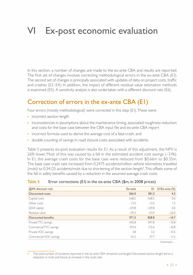
In this section, a number of changes are made to the ex-ante CBA and results are reported. The first set of changes involves correcting methodological errors in the ex-ante CBA (E1). The second set of changes is principally associated with updates of data on project costs, traffic and crashes (E2–E4). In addition, the impact of different residual value estimation methods is examined (E5). A sensitivity analysis is also undertaken with a different discount rate (E6).

Correction of errors in the ex-ante CBA (E1)Four errors (mostly methodological) were corrected in this step (E1). These were:

4 The total number of accidents reported in the ex-ante CBA remained unchanged. Decreased section length led to a reduction in mvkt and hence an increase in the crash rate.

• incorrect section length• inconsistencies in assumptions about the maintenance timing, associated roughness reduction

and costs for the base case between the CBA input file and ex-ante CBA report• incorrect formula used to derive the average cost of a fatal crash, and • double-counting of savings in road closure costs associated with accidents.

Table 5 presents ex-post evaluation results for E1. As a result of this adjustment, the NPV is 26% lower. Most of this was caused by a fall in the estimated accident cost savings (–31%). In E1, the average crash costs for the base case were reduced from $0.66m to $0.35m. The base case crash rate increased from 0.2475 accidents/million vehicle kilometres travelled (mvkt) to 0.34125 accidents/mvkt due to shortening of the section length4. This offsets some of the fall in safety benefits caused by a reduction in the assumed average crash costs.

Table 5 Error corrections (E1) in the ex-ante CBA ($m, in 2008 prices)

@4% discount rate Ex-ante E1 E1/Ex-ante (%)


Capital costs 568.5 568.5 0.0Other costs –13.3 –13.5 1.5QWI capital –129.8 –129.8 0.0Residual value –59.3 –43.9 –26.0Discounted benefits 971.3 828.8 –14.7

Private TTC savings 445.8 397.8 –10.8Commercial TTC savings 193.4 172.6 –10.8Private VOC savings 3.8 3.2 –15.5Commercial VOC savings 42.5 37.7 –11.2

Continued…

• 26 •


@4% discount rate Ex-ante E1 E1/Ex-ante (%)

Accident savings 194.9 134.8 –30.8Road closure savings 8.2 0.0 –100.0Flood closure savings 82.7 82.7 0.0Net present value (NPV) 605.2 447.5 –26.1

Benefit-cost ratio (BCR) 2.65 2.17

FYRR 5.74% 3.13%

Correcting the section length from 13km to 11.6km seems a small change but is in fact a 10.77% reduction in length. As the major savings arise from travel time costs (TTC) and vehicle operating costs (VOC), which are dependent on MVKT, this correction led to a fall in TTC and VOC savings by 11–16%. The errors corrected in this step could have been avoided if a peer review had been undertaken.

The FYRR is also corrected here to include the omitted first-year flooding costs as discussed above in the section titled ‘Review of ex-ante CBA’. The FYRR reported in the 2009 ex-ante CBA of 5.74% was reduced to 3.83% in the corrected ex-ante CBA. After E1 corrections the FYRR fell to 3.13%.

Updating projects costs (E2)The amendments made in this step (E2) included updating the project capital costs and setting QWI’s contribution to zero. The discounted actual spending on the project was $375m, 34% below the budgeted costs (table 6). As discussed earlier, these cost reductions were caused mostly by the reduced project scope due to the cancellation of the Traveston Dam project and to a lesser extent by increasing market competition in the construction industry as a result of the global financial crisis, the end of the mining boom and improvements in project design. As a result of this adjustment, NPV increased by 16% with BCR rising from 2.17 to 2.67 (at the 4% discount rate).

Table 6 Updating project costs (E2) ($m, in 2008 prices)

@4% discount rate E1 E2 E2/E1 (%)

Discounted costs 381.3 310.6 –18.5

Capital costs 568.5 375.0 –34.0Other costs –13.5 –13.5 0.0QWI capital –129.8 0.0 –100.0Residual value –43.9 –50.9 15.8Discounted benefits 828.8 828.8 0.0

Private TTC savings 397.8 397.8 0.0Commercial TTC savings 172.6 172.6 0.0Private VOC savings 3.2 3.2 0.0Commercial VOC savings 37.7 37.7 0.0Accident savings 134.8 134.8 0.0Road closure savings 0.0 0.0 0.0Flood closure savings 82.7 82.7 0.0Net present value (NPV) 447.5 518.2 15.8


FYRR 3.13% 4.75%

• 27 •

Appendix B.1 • VI Ex-post economic evaluation

Updating traffic forecasts (E3)This step (E3) updates initial traffic level, traffic growth and traffic composition. Key elements of the change included:

5 In QDTMR (2011), it is assumed a road’s ‘maximum capacity’ is reached when the volume-capacity ratio (VCR) reaches 1.25 (operating speed falls to 30km/h). The volume is calculated using annual average daily traffic, which is converted into passenger car units. The capacity is adjusted using a capacity factor (=10% for the national highway) to include the impacts of peak traffic flow. Peak periods can be considered congested when maximum capacity is reached, but the costs of congestion are calculated as if they are evenly distributed across the day. This method over-states the congestion impact.

• a reduction in the initial traffic level from 16,000 vehicles a day to 14,736 vehicles a day• a reduction in the assumed growth rate from 3% to 2.17% a year (linear)• an increase in the share of commercial vehicles from 15% to 27%, and • a reduction in the bus share from 3% to 1%.

As seen in table 7, the impact of this update is quite large with the NPV dropping by 62%. The fall in TTC savings was largely responsible for this drop. The lower AADT and lower traffic growth rates delay the onset of congestion in the base case. In the ex-ante CBA, traffic in peak hours reaches maximum base case capacity in year 20. In the ex-post CBA, this is postponed to 295. Consequently, the estimated BCR for the project falls from 2.67 to 1.58, which shows that modest changes in traffic growth and traffic composition can have large impacts on the bottom-line results.

Table 7 Updating traffic forecasts (E3) ($m, in 2008 prices)



Capital costs 375.0 375.0 0.0Other costs –13.5 –13.5 0.0QWI capital 0.0 0.0 0.0Residual value –50.9 –19.5 –61.8Discounted benefits 828.8 540.2 –34.8

Private TTC savings 397.8 200.3 –49.7Commercial TTC savings 172.6 121.1 –29.9Private VOC savings 3.2 –1.4 –143.1Commercial VOC savings 37.7 29.8 –20.9Accident savings 134.8 121.9 –9.6Road closure savings 0.0 0.0 0.0Flood closure savings 82.7 68.5 –17.2Net present value (NPV) 518.2 198.2 –61.8


FYRR 4.75% 4.38%

• 28 •


Updating crash forecasts (E4)Step E4 updates crash forecasts for the project. It was pointed out previously (see table 3) that the updated crash rate for the base case was an under-estimate due to the problem associated with the ex-post crash data (missing crash data for 1km of the project section length). The key changes introduced in E4 are summarised in table 8. As seen, both the updated accident rate and average accident costs for the base case under E4 are substantially lower than those for the ex-ante analysis or E1. This adjustment resulted in a substantial fall in safety benefits (–86% compared with ex-ante results and –78% compared with E3 (table 7)). While there were uncertainties about the updated crash forecasts for the base case, the significant difference between the ex-ante and ex-post safety results suggests there may be a need to improve safety analysis in road CBAs.

Table 8 Accident rates and average accident costs

Ex-ante E1 E4

Base case Project case Base case Project case Base case Project case

Accident rates (accidents/mvkt) 0.2475 0.1210 0.3412 0.1210 0.1808 0.1210Average accident costs ($/accident) $660,073 $258,165 $345,572 $258,165 $287,070 $258,165

Source: provided by QDTMR (2015) for this case study.

Table 9 Updating crash forecasts (E4) ($m, in 2008 prices)



Capital costs 375.0 375.0 0.0Other costs –13.5 –13.5 0.0QWI capital 0.0 0.0 0.0Residual value –19.5 –9.1 –53.2Discounted benefits 540.2 445.2 –17.6

Private TTC savings 200.3 200.3 0.0Commercial TTC savings 121.1 121.1 0.0Private VOC savings –1.4 –1.4 0.0Commercial VOC savings 29.8 29.8 0.0Accident savings 121.9 26.9 –77.9Road closure savings 0.0 0.0 0.0Flood closure savings 68.5 68.5 0.0Net present value (NPV) 198.2 92.8 –53.2


FYRR 4.38% 3.25%

• 29 •


Change in the estimation methods for RVs (E5)Up to E4, the RVs have been estimated using the incorrect annuity approach adopted in the ex-ante CBA. This step (E5) involves testing the impact on CBA results of updated RV estimates derived from different methodologies (see appendix E in the main report).

The first set of tests involved use of the RV derived from the straight line depreciation as recommended by QDTMR and applying it both as a cost and benefit item in CBA calculations. As seen in table 10, the estimated RV based on straight line depreciation is significantly higher than that derived from the incorrect ex-ante methodology. Treating the derived RV either as a cost or a benefit item would not change the NPV, but would lead to different BCRs (1.41 as a cost item and 1.36 as a benefit item).

The second set of tests involved using the RVs derived from the variants of the net benefit stream approach and applying them as a benefit item only in CBA calculations. Figure 2 is a summary of the annual net benefit projections based on the four variants of the benefit stream approach, namely: • B0: the annuity taken of the PV of net benefits over the analysis period and extrapolated

into future years• B1: decreasing net benefits at equivalent 5% (= 100% / 20 years) a year (linear) • B2: constant net benefits over time• B3: increasing net benefits in line with the growth in traffic (2.17% a year, linear).

Also shown in figure 2 are the predicted speeds for cars for both the base and project cases on the right-hand scale. These speed curves are included to help understand how the net benefits evolve over and beyond the evaluation period. As illustrated, the speed for the base case beyond year 30 is largely driven by an arbitrary queuing speed assumption (30km/h). With a further reduction in the modelled speed for the project case, travel time savings per private car will become smaller over time as the new road also becomes congested.

• 30 •

BITRE • Report 145 Volume 2 Case StudiesTa

ble

10

Cha

nge

in R

V e

stim

atio

n m

etho

dolo

gies

(E5)

($m

, in

2008

pri

ces)

E4E5

Ex-a

nte

appr

oach

E5.1

Stra

ight

line

dep

reci

atio

nE5

.2 N

et b

enefi

t st

ream

app

roac

h

(Inco

rrec

t an

nuity

fo

rmul

a)C

1 (a

s a

cost

item

)C

2 (a

s a

bene

fit it

em)

B 0 (a

nnui

ty)

B 1 (D

imin

ishi

ng n

et

bene

fits)

B 2 (C

onst

ant

net

bene

fits)

B 3 (In

crea

sing

net

be

nefit

s)

Dis

coun

ted

cost

s 35

2.4

316.

836

1.5

361.

536

1.5

361.

536

1.5

Capi

tal c

osts

375.0

375.0

375.0

375.0

375.0

375.0

375.0

Oth

er co

sts

–13.5

–13.5

–13.5

–13.5

–13.5

–13.5

–13.5

QW

I cap

ital

0.00.0

0.00.0

0.00.0

0.0Re

sidua

l valu

e–9

.1–4

4.6(R

V as

% o

f tot

al co

sts)

2.614

.1D

isco

unte

d be

nefit

s 44

5.2

445.

248

9.8

535.

261

2.6

755.

481

7.4

Priva

te TT

C sa

vings

20

0.320

0.320

0.320

0.320

0.320

0.320

0.3Co

mm

ercia

l TTC

savin

gs

121.1

121.1

121.1

121.1

121.1

121.1

121.1

Priva

te V

OC

savin

gs

–1.4

–1.4

–1.4

–1.4

–1.4

–1.4

–1.4

Com

mer

cial V

OC

savin

gs

29.8

29.8

29.8

29.8

29.8

29.8

29.8

Accid

ent s

aving

s 26

.926

.926

.926

.926

.926

.926

.9Ro

ad cl

osur

e sa

vings

0.0

0.00.0

0.00.0

0.00.0

Flood

clos

ure

savin

gs

68.5

68.5

68.5

68.5

68.5

68.5

68.5

Resid

ual v

alue

44.6

90.0

148.3

274.9

337.6

(RV

as %

of t

otal

bene

fits)

9.116

.825

.038

.243

.1N

et p

rese

nt v

alue

(NPV

)92

.812

8.4

128.

417

3.7

231.1

358.

742

1.3

Bene

fit-c

ost

ratio

(BC

R)

1.26

1.41

1.36

1.48

1.64

1.99

2.17

• 31 •


Figure 2 Annual net benefit projections

As expected, RV estimates based on the different methods of projecting the benefit stream forward vary significantly (see E5.2 of table 10). The annuity approach (B0) produces the lowest estimate of RV. The constant (B2) and increasing (B3) net benefit assumptions cause the estimated RVs to comprise very high shares of the total road user benefits (40–45%), which appear unreasonably high. The RV derived from the diminishing net benefit approach (B1) might be considered the most plausible as it is the most conservative with the most credible assumptions (see appendix E in the main report). The NPV based on the RV derived from the diminishing net benefit approach was estimated to be $231m, compared with $128m derived from the straight line depreciation.

Change in the discount rate (E6)Step E6 involves a sensitivity test to change the discount rate from 4% to 7%. As seen from table 11, increasing the discount rate to 7% reduces benefits by 44%. The components most affected are RV, commercial and private TTC savings and commercial VOC savings, which have decreased by 63.0%, 46.5% and 41.1% respectively. The NPV has become negative and the BCR well below 1. The higher discount rate has made the project economically unviable.

Table 11 Change in the discount rate (E6) ($m, in 2008 prices)

E5.1 (@4%) E6 (@7%)

Discounted costs 316.8 313.8

Capital costs 375.0 343.7Other costs –13.5 –12.9QWI capital 0.0 0.0

Continued…

$0.00

$20.00

$40.00

$60.00

$80.00

$100.00

$120.00

0

20

40

60

80

100

120

B1 (-5% pa)B0 Annuity

B3 (2.17% pa)B2 (0% pa)Project Case Speed

Base speedNet Benefits

Net

Ben

efits

($m

)

Priv

ate

Car

Ope

ratin

g Sp

eed

(km

/h)

2008 206820582048203820282018

Year (Project completed in 2012)

• 32 •


E5.1 (@4%) E6 (@7%)

Residual value –44.6 –17.0Discounted benefits 445.2 247.8

Private TTC savings 200.3 108.1Commercial TTC savings 121.1 63.7Private VOC savings –1.4 –0.9Commercial VOC savings 29.8 17.6Accident savings 26.9 16.7Road closure savings 0.0 0.0Flood closure savings 68.5 42.6

Net present value (NPV) 128.4 –66


FYRR 3.25% 3.08%

SummaryTo bring together the ex-post evaluation results, the components of the total variation in NPV between the ex-ante and ex-post CBAs are set out in figure 3. Using the straight-line depreciation method for the RV, the ex-post NPV was estimated to be $128m, implying the project is economically viable at the 4% discount rate. However, the updated NPV was $477m or 79% lower than the ex-ante estimate. Causes for this shortfall were overly optimistic traffic forecasts (E2–E3, –67%), miscellaneous errors (mostly methodological) made in the ex-ante CBA (EA–E1, –33%) and over-estimation of safety benefits (E3–E4, –22%). Lower actual project costs offset some of the fall in NPV. Changing the RV estimation method to straight line depreciation made a positive contribution. The sensitivity test showed that at a 7% discount rate the project became economically unviable.

Figure 3 Sources of variations in NPV

-350

-300

-250

-200

-150

-100

-50

0

50

100

$m


E3-E4(Crash Updates)

E2-E3(Traffic Updates)

E1-E2(Actual Costs & QWI)

EA-E1(Method Correction)

NPV (ex-ante) = $604mNPV (ex-post) = $128m

-157.7

70.7

-320.0

-105.3

35.5

• 33 •

VII Lessons learned

This final section draws out the lessons for future economic evaluation from the review of the ex-ante CBA and the ex-post evaluation.

DocumentationDocumentation for the ex-ante CBA was excellent including the main CBA report, CBA6 software and associated user manual and CBA6 model input files. Good documentation increases transparency, facilitates peer review and lowers costs for ex-post evaluation. QDTMR is commended for keeping good CBA records.

Review of ex-ante CBAA number of errors were found in the ex-ante CBA through the ex-post review. Some of these could have been avoided if a thorough review had been undertaken. For example, the CBA results in the ex-ante analysis showed an extremely high proportion of total travel time savings accruing to buses, which would have been spotted by a careful reviewer. Section length is another example of an error that could have easily been avoided. Other errors, such as the calculation of the cost per fatal crash, could only be found by reviewing the spreadsheet calculations behind the CBA report.

Errors found during the review stage of this ex-post evaluation could have been detected and avoided if a peer review process had been in place. There is no formal expert review process for CBAs of national road investment projects at the federal level. Establishment of such a process would provide timely feedback on, and improve the quality of, ex-ante CBAs.

CBA of mutually dependent projectsConstruction of the Traveston Dam and the upgrade of the Bruce Highway were related projects in that implementation of one increases the costs of the other. In an ideal situation, these two projects should have been evaluated jointly with the option of implementing both together compared with the options of implementing each in isolation. In case this was not possible, a rationale should have been provided for treating the QWI’s payment as a negative cost. Such information would be useful for determining the plausibility of the underlying assumptions.

• 34 •


Significant over-estimation of project costsThere was a significant over-estimation of project costs due to the cancellation of the dam project and easing of the road construction market. Detailed review of each cost item would be required to identify the specific factors causing the cost over-estimation, which would be beyond the scope of the present study.

Traffic forecastsRoad user benefits are closely related to the assumed initial level of traffic and its forecast growth. The initial traffic level and forecast traffic growth in the original analysis were over-estimated. Forecasts for traffic on non-urban roads are difficult to make because of inadequate traffic count data from past years. Our update of the traffic forecast for this ex-post evaluation was based on simple trend extrapolation. In future, whenever possible, more data should be collected to allow for more sophisticated traffic modelling, such as multivariate regression analyses that include the effects of growth in income and population in the study area. BITRE forecasts for non-urban corridors can be also used as a source of comparison and sensitivity tests. The BITRE forecasts were made treating freight and cars separately.

Changing the traffic composition had an important bearing on the evaluation results. In the ex-ante analysis, the assumption of a fixed traffic composition led to a large under-representation of commercial vehicles in the fleet over the study period. Relaxing the assumption of a fixed traffic composition could pose a challenge to traffic forecasters as they would have to forecast separately the AADTs for major vehicle categories.

Crash analysisQuite significant errors were found in the ex-ante CBA in the estimation of unit crash costs and the crash rate for the base case. These errors could have been avoided if more scrutiny had been undertaken of the CBA6 model inputs.

Attempts to update the base case crash forecast for this ex-post evaluation were hampered by the lack of good and reliable crash data. Until the data problems are solved, both ex-ante and ex-post economic evaluators will continue to face serious challenges in improving the accuracy of the estimated safety benefits.

Residual valuesCurrently two approaches are generally used for estimating RV, the straight line depreciation and net benefit approaches. Each approach has pros and cons. Conceptually, net benefit approaches are more attractive because they relate the value of an asset to the benefit it is able to generate. However, in practice, straight-line depreciation is used more because it is conservative. For most projects with a BCR above one, the straight line depreciation approach provides a lower bound for RV estimates and the benefit approach an upper bound.

RVs derived from the net benefit approaches are subject to significant uncertainties associated with the asset life, the discount rate used, long-term traffic forecasts, maintenance and renewal costs and changes in the base case in the distant future. For this reason, the European Commission

• 35 •

Appendix B.1 • VII Lessons learned

(EC 2014) recommended use of the depreciation approach for projects with very long design lives as, often occurs in the transport sector. The findings of this case study support the EC (2014) recommendation. RVs derived from the net benefit stream approach in this case study were found to be so large that they could distort economic analysis if adopted.

If the net benefit approach is to be encouraged for use in RV derivation, general guidelines will be necessary. Without them, there is a substantial risk of over-estimating RV for road projects.

As to whether RVs derived from asset depreciation should be treated as a cost or benefit item in road CBA, if the BCR is needed to rank the projects according to the return per dollar currently invested, RV should be treated as a net benefit at the end of the evaluation period. In this case, the depreciated cost is being used as a proxy for future project benefits beyond the end of the evaluation period.

To cater for diverse views on defining the BCR, it is recommended that BCRs with different definitions be clearly marked as such.

• 37 •

References (additional)

Austroads 2012, Guide to Project Evaluation. Part 2 Project Evaluation Methodology , https://www.onlinepublications.austroads.com.au/items/AGPE02–12.

Haraldsson, M. and L. Jonsson 2012, Estimating the Economic Lifetime of Roads Using Road Replacement Data, May. https://ideas.repec.org/p/hhs/vtiwps/2008_005.html.

QDTMR 2008a, Project Proposal Report: Scoping, Development and Delivery Phases – Bruce Highway Upgrade Cooroy to Curra Section B (Sankeys Road to Traveston Road), December 2008.

QDTMR 2008b, Cost–Benefit Analysis – Bruce Highway Upgrade Cooroy to Curra Section B, Project 128/10A/31, November 2008.

QDTMR 2015, Ex-post Cost Benefit Analysis, internal paper, February.



Dampier Highway Upgrade – Broadhurst Road to Burrup Peninsular Road

Appendix B.2


• 41 •

Contents

Summary ......................................................................................................................................................................47

I Introduction .................................................................................................................................................................49

II Description of the Dampier Highway upgrade project ...................................................................51

III Review of ex-ante CBAs .....................................................................................................................................53

IV Methodological issues in ex-post evaluation ..........................................................................................55

Traffic updates ......................................................................................................................................55

Road user cost estimation .............................................................................................................58

Project costs ..........................................................................................................................................60

Residual values .....................................................................................................................................60

First-year rate of return (FYRR) .................................................................................................61

Base and price year ...........................................................................................................................63

Discount rate ........................................................................................................................................63

V Reconstruction of the ex-ante CBAs .........................................................................................................65

VI Ex-post economic evaluation ...........................................................................................................................67

Stage 1B: Project costs (E1) ...........................................................................................................67

Stage 1B: Traffic update (E2) .........................................................................................................67

Stage 1B: Residual values (E3) ......................................................................................................68

Stages 2–6: Project costs (E1) ......................................................................................................69

Stages 2–6: Traffic updates (E2) ..................................................................................................69

Stages 2–6: Residual values (E3) .................................................................................................70

Sensitivity analysis ...............................................................................................................................70

Summary .................................................................................................................................................72

VII Lessons learnt ............................................................................................................................................................75

Documentation ...................................................................................................................................75

Review of ex-ante CBAs ................................................................................................................75

Traffic forecasting in a volatile area ..........................................................................................75

• 42 •


Crash analysis ........................................................................................................................................76

Business case for cycle lanes ........................................................................................................76

Residual values .....................................................................................................................................76

First-year rate of return .................................................................................................................77

Appendix A: Traffic demand analysis ..................................................................................................................79

References (additional) .....................................................................................................................................................85

• 43 •

List of tables

Table 1 Ex-ante CBA for the Dampier Highway upgrade project ($m) .............................53

Table 2 Updated ex-ante CBA for the Dampier Highway upgrade project (Stages 2–6) ...........................................................................................................................................54

Table 3 Corrected ex-ante CBA for the Dampier Highway upgrade project .................54

Table 4 Recent growth trends in traffic on the Dampier Highway (AADT) ....................55

Table 5 Forecast population and traffic growth rates (% a year) .............................................56

Table 6 Traffic composition (%) ...................................................................................................................57

Table 7 Estimation of asset life for stage 1B ..........................................................................................61

Table 8 First-year rate of return (@4%)..................................................................................................61

Table 9 Updating project costs – stage 1B (E1) ..................................................................................67

Table 10 Traffic update – stage 1B (E2) .....................................................................................................68

Table 11 Including residual values – stage 1B (E3) ...............................................................................68

Table 12 Updating project costs – stages 2–6 (E1) .............................................................................69

Table 13 Updating traffic forecasts – stages 2–6 (E2) .......................................................................69

Table 14 Including residual values – stages 2–6 (E3) ..........................................................................70

Table 15 Sensitivity tests of alternative traffic growth scenarios .................................................70

Table 16 Sensitivity test of alternative discount rate ..........................................................................71

Table A1 Recent growth trends in traffic on Dampier Highway (AADT) .............................79

Table A2 Data used in regression analysis .................................................................................................81

Table A3 Regression results ...............................................................................................................................81

Table A4 Population growth forecasts .......................................................................................................82

• 45 •

List of figures


Figure 1 Proposed Dampier Highway upgrade ....................................................................................52

Figure 2 Recent traffic counts adjacent to Madigan Road .............................................................57

Figure 3 Crash rates along the Dampier Highway for Stages 1B and 2–6 (crashes per million vehicle kilometres travelled) ............................................................58

Figure 4 Optimal implementation year for stage 1B and stages 2–6 (ex-ante) .................62

Figure 5 Sources of variation in NPV for stage 1B and stages 2–6 ...........................................73

Figure A1 Location map ........................................................................................................................................80

Figure A2 Traffic demand as a function of population .........................................................................82

Figure A3 Comparisons of traffic forecasts ................................................................................................83

• 47 •

Summary

The Bureau of Infrastructure, Transport and Regional Economics (BITRE) is undertaking a second round of ex-post evaluations of national road investment projects. This case study was a joint effort between BITRE and Main Roads Western Australia (MRWA) to assess the economic performance of the Dampier Highway upgrade project and to check the accuracy of the ex-ante cost-benefit analysis (CBA) undertaken for the project.

The Dampier Highway upgrade involved duplication to four lanes of the 15.2 kilometre section between Karratha and Dampier in the Pilbara region of Western Australia. The project has two components: stage 1B to duplicate the road between Broadhurst Road to Balmoral Road West (2.9km completed in October 2009) and stages 2–6 between Balmoral Road West and Burrup Road (12.3km completed in February 2013).

In the ex-post evaluation, actual project costs were lower than budgeted costs after discounting for both stage 1B and stages 2–6. In contrast, traffic forecasts were grossly over-estimated leading to excessive road user benefits. The ex-ante analysis did not consider the residual values (RVs) of the projects. Altogether, three adjustments were made in this ex-post evaluation to the ex-ante CBA: E1. adjusting project costs E2. updating traffic forecasts, andE3. including RVs as additional benefits to road users.

Figure E.1 summarises the impact of these adjustments on the project’s net present value (NPV). The updated NPV for stage 1B was 91% below the ex-ante estimate while the NPV for stages 2 to 6 became negative, indicating the project was economically unviable. The main contributor to the fall was the correction of overly optimistic traffic forecasts (E2) which reduced the NPV by $17.3m for stage 1B and by $167.2m for stages 2–6. The project cost update (E1) offset slightly some of this fall in NPV for both projects. Inclusion of the RVs (E3) increased the NPV by $1.3m for stage 1B and by $10.3m for stages 2 to 6. The revised benefit-cost ratio (BCR) for stage 1B and stages 2–6 are 1.12 and 0.50 respectively (from 2.08 and 2.32).

• 48 •




The first-year rate of return (FYRR) estimated in both the ex-ante and ex-post analyses was below 4% for both projects indicating both investments should have been delayed. Sensitivity tests of alternative traffic growth scenarios showed that the stage 1B project would not be economically viable if the low traffic growth scenario (1.2% a year) was to eventuate; and even with high traffic growth (3.6% a year), stages 2–6 would remain uneconomical. Increasing the discount rate from 4% to 7% made both stage 1B and stages 2–6 economically unviable.

Key lessons learnt from this case study include:• Forecasting traffic for projects in a volatile area requires a greater effort to understand the

nature of the observed trend. This is especially true when long-term time-series data are not available and the trend extrapolation method has to be used for forecasting. If there are uncertainties, scenario tests should be conducted to better inform decision makers.

• Crash analysis in volatile areas may be influenced by temporary factors, which could lead to a bias in the estimated crash rate for the base case. Wherever possible, site-specific crash rates should be calculated using data over a longer period of time to ensure short-term effects are removed. In the absence of good data and sound analysis, it may be preferable to use generic crash rates for different road conditions as recommended by Austroads.

• A business case should be established for adding cycle lanes alongside a national highway through an incremental CBA.

• The first year rate of return (FYRR) metric is essential to the inter-temporal maximisation of investment returns. FYRR reporting should be compulsory for future road project CBAs. A FYRR test will help determine the best timing for investment.

-180

-160

-140

-120

-100

-80

-60

-40

-20

0

20

Stages 2-6Stage 1B

E2-E3 (Residual Value)E1-E2 (Traffic update)E1-E2 (Project costs)

$m

2.80 1.95

-17.27

-167.19

1.3110.30

Stage 1B NPV (ex-ante) = $14.48mStage 1B NPV (ex-post) = $1.3mStages 2–6 NPV (ex-ante) = $113.16mStages 2–6 NPV (ex-post) = –$41.8m

• 49 •

I Introduction

The Dampier Highway case study forms part of the second round of ex-post cost-benefit analysis (CBA) undertaken by the Bureau of Infrastructure, Transport and Regional Economics (BITRE) on national road investment projects. This case study was a joint effort between BITRE and Main Roads Western Australia (MRWA) to:• assess the economic performance of the project• check the accuracy of ex-ante CBA’s predictions• explain differences (if any) in results between the ex-ante and ex-post CBAs, and • draw lessons from the case study to improve future CBAs.

Issues associated with traffic forecasting in a volatile area, such as the Pilbara region, are also investigated, as are the implications of volatility on project timing. Cycle lane benefits and the residual value (RV) of the project, which were not considered in the ex-ante CBA, are explored. Disaggregate analysis of the Dampier Highway duplication shows that benefits may be concentrated in only a part of the road duplication.

The following section provides an overview of the Dampier Highway – Broadhurst Road to Burrup Peninsular Road upgrade project for stages 1B and 2–6. Section 3 reviews the ex-ante CBAs undertaken by MRWA. Methodological issues for the ex-post evaluation are discussed in Section 4. Section 5 reconstructs the ex-ante analysis using the original version of Western Australia’s Road Evaluation System (WARES). Section 6 presents ex-post evaluation results. Lessons learnt are discussed in the last section.

• 51 •

II Description of the Dampier Highway upgrade project

The Dampier Highway Upgrade project involved duplication to four lanes of the 15.2 kilometre section of the Dampier Highway between Karratha and Dampier in the Pilbara region of Western Australia. The project comprised two components: stage 1B that involved duplication of the road between Broadhurst Road to Balmoral Road West (2.9km), and stages 2–6 between Balmoral Road West and Burrup (12.3km) (figure 1). Key features of the project included: • A new carriageway of the duplicated highway to run parallel to the existing road on the

western side of the existing carriageway. Across the salt flats, the alignment would be on the eastern side of the existing carriageway.

• Alignment of the duplication passes across Seven Mile Creek where a bridge would be built parallel to the existing bridge. The existing bridge would be strengthened and the guard rail modified.

• Introduction of 2 metre wide cycle lanes on both directions of the highway. A rumble strip would separate the outer carriageway and cycle lane.

The total budgeted cost for stage 1B was $13.4m (in 2009 prices) and, for stages 2–6, $85.5m (in 2009 prices). The actual project cost for stage 1B was $10.6m (in 2009 prices) and that for stages 2–6 was $97.1m (nominal) or $91.1m (in 2009 prices).

Stage 1B was completed in October 2009. Stages 2–6 were commenced in January 2011 and completed in February 2013.

• 52 •


Figure 1 Proposed Dampier Highway upgrade

Source: MRWA (2009a).

• 53 •

III Review of ex-ante CBAs

The first CBA was undertaken by MRWA in March 2009 and its results were reported in the first project proposal report (PPR) for the Dampier Highway Duplication project (MRWA 2009a). Table 1 reproduces the key CBA results.

Table 1 Ex-ante CBA for the Dampier Highway upgrade project ($m)

Stage 1B

Discount rate

4% 7%

Benefits 25.57 14.81

Vehicle operating costs 5.82 3.62Accident costs 5.77 3.73Travel time costs 13.92 7.45Maintenance costs 0.06 0.01Benefit-cost ratio 2.08 1.20

Stages 2–6

Discount rate

4% 7%

Benefits 191.26 103.52

Vehicle operating costs 27.91 16.55Accident costs 9.16 5.18Travel time costs 155.41 82.64Maintenance costs –1.22 –0.85Benefit-cost ratio 1.81 0.98

1 WARES is a compiled program used to evaluate rural roads in WA.

Source: MRWA (2009a).

The benefits were estimated using Western Australia’s Road Evaluation System (WARES)1 with a 30-year evaluation period. Key benefit categories were reduction in travel time and vehicle operating costs, improved safety, and less need for longer-term maintenance. Based on a 4% discount rate, the benefit-cost ratio (BCR) for Stage 1B was estimated at 2.08 (based on a construction cost of $13.4m in 2009 prices) and for Stages 2–6, 1.81 (based on a construction cost of $115m in 2009 prices). Discounted project costs were not reported in the PPR (2009a).

In December 2009, MRWA (2009b) lodged the second PPR revising construction costs for stages 2–6 from $115m down to $85.5m (in 2009 prices). As a result, BCR for Stages 2–6 became higher (table 2). Again discounted costs were not reported.

• 54 •


Table 2 Updated ex-ante CBA for the Dampier Highway upgrade project (Stages 2–6)

($m)

Discount rate

4% 7%

Benefits 182.25 98.84

Vehicle operating costs 28.24 16.82Accident costs 8.77 4.95Travel time costs 146.47 77.93Maintenance costs –1.22 –0.85Benefit-cost ratio (BCR) 2.14 1.16

Source: MRWA (2009b).

A crosscheck of the WARES output revealed that the benefits reported in tables 1 and 2 were under-estimated as they were expressed in 2007 (not 2009) prices. In WARES, a price adjustment was automatically made to the calculated project BCR but not to the reported user benefits. The latter should have been adjusted outside the WARES calculation using a conversion factor of 9% (increases in prices between 2007 and 2009) for reporting in the PPR. Table 3 reports both the costs and benefits associated with the project in 2009 prices. The discounted costs were derived from total discounted benefits and the reported BCR. The incorrect BCR for stages 2–6 reported in table 2 was also corrected as it was based on 2007 prices.

Table 3 Corrected ex-ante CBA for the Dampier Highway upgrade project

Stage 1B

($m, in 2009 prices)

Discount rate

4% 7%

Benefits 27.87 16.14

Vehicle operating costs 6.34 3.95Accident costs 6.29 4.06Travel time costs 15.18 8.12Maintenance costs 0.07 0.01Construction costs 13.40 13.40Benefit-cost ratio 2.08 1.20

Stages 2–6

($m, in 2009 prices)

Discount rate

4% 7%

Benefits 198.65 107.74

Vehicle operating costs 30.78 18.33Accident costs 9.56 5.40Travel time costs 159.65 84.94Maintenance costs –1.33 –0.93Construction costs 85.5 85.5Benefit-cost ratio 2.32 1.26

Since the CBAs for stage 1B in MRWA (2009a) and stages 2–6 in MRWA (2009b) were the basis on which the final decisions were made to proceed with the project, they were the focus in our ex-post evaluation.

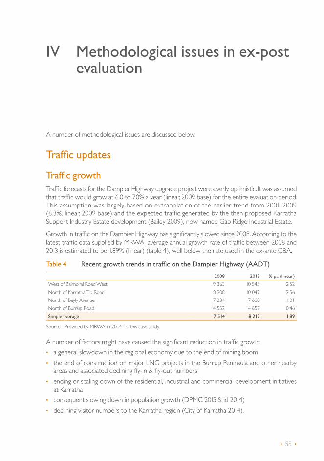
• 55 •


A number of methodological issues are discussed below.

Traffic updates

Traffic growthTraffic forecasts for the Dampier Highway upgrade project were overly optimistic. It was assumed that traffic would grow at 6.0 to 7.0% a year (linear, 2009 base) for the entire evaluation period. This assumption was largely based on extrapolation of the earlier trend from 2001–2009 (6.3%, linear, 2009 base) and the expected traffic generated by the then proposed Karratha Support Industry Estate development (Bailey 2009), now named Gap Ridge Industrial Estate.

Growth in traffic on the Dampier Highway has significantly slowed since 2008. According to the latest traffic data supplied by MRWA, average annual growth rate of traffic between 2008 and 2013 is estimated to be 1.89% (linear) (table 4), well below the rate used in the ex-ante CBA.

Table 4 Recent growth trends in traffic on the Dampier Highway (AADT)

2008 2013 % pa (linear)

West of Balmoral Road West 9 363 10 545 2.52North of Karratha Tip Road 8 908 10 047 2.56North of Bayly Avenue 7 234 7 600 1.01North of Burrup Road 4 552 4 657 0.46Simple average 7 514 8 212 1.89

Source: Provided by MRWA in 2014 for this case study.

A number of factors might have caused the significant reduction in traffic growth:• a general slowdown in the regional economy due to the end of mining boom• the end of construction on major LNG projects in the Burrup Peninsula and other nearby

areas and associated declining fly-in & fly-out numbers• ending or scaling-down of the residential, industrial and commercial development initiatives

at Karratha• consequent slowing down in population growth (DPMC 2015 & id 2014) • declining visitor numbers to the Karratha region (City of Karratha 2014).

• 56 •


One significant source of over-estimation of traffic demand was from the Karratha Support Industry Estate (KSI) initiative (now called Gap Ridge Industrial Estate), which was developed by the LandCorp land development agency. Traffic modeling undertaken by Transcore (2009) assumed the development would occur in four stages commencing in 2009 and ending in 2021. The additional traffic generated by this development was estimated to be 2,670 vehicles a day by 2011 (stage 1), 4,757 by 2016 (stage 2) and 9,753 by 2021 (stage 4) using the trip generation rates2 recommended by the NSW Guide to Traffic Generating Developments (RTA 2002).

So far the KSI has not been released in the planned stages. Instead the land for all stages has been released concurrently according to LandCorp (2015a). While the KSI is currently at planned capacity (�49%) based on a recent lot plan (LandCorp 2015b), anecdotal observations made during the site visit3 undertaken for this evaluation revealed that the KSI had not been generating traffic as planned. Further investigation is required before the reasons for this can be identified.

Updating traffic forecasts for this case study faces no fewer challenges than for the ex-ante traffic analysis. Limited availability of historical data on traffic counts has prevented any robust quantitative analysis. A combination of simple quantitative methods and qualitative judgments were applied to form an updated view about the future traffic growth.

In modeling the future traffic, consideration of the availability of forecasts for potential exogenous variables led to a model specification that links traffic demand to the population only.

Recent population forecasts at the more aggregate level point to an approximate 2% a year compound growth for the Karratha region (Australian Bureau of Statistics 2014, Department of the Prime Minister and Cabinet 2015). For the purpose of this ex-post evaluation, population forecasts made by the Western Australian Planning Commission (WAPC 2012) were considered particularly relevant because they included a central population forecast with a range over the period from 2006 to 2026. Table 5 summarises traffic growth forecasts based on the regression model under the three different population growth scenarios specified by WAPC (2012). The traffic growth rate under the central scenario was forecast to be 2.4% a year with 1.2% as a lower bound and 3.6% as an upper bound. These updated growth rates were all well below the growth rate (6.0–7.0% a year) assumed in the ex-ante CBAs.

Table 5 Forecast population and traffic growth rates (% a year)

Lower Central Upper

Population (WAPC 2012)(compound) 0.5 1.4 2.1Traffic (linear) 1.2 2.4 3.6

Traffic growth in the recent past has been slower than that for the central scenario, however it is within the bounds of the forecast range. In the short term, possibilities cannot be ruled out that the actual traffic growth may move outside the forecast range. This has already been observed from the volumes recorded by a traffic counter north of Madigan Road as plotted along with traffic counts produced in the ex-ante traffic analysis on the Dampier Highway to the west of Madigan road in figure 2.

2 RTA (2002) recommends a trip rate of five vehicles a day for each factory and four vehicles a day for 100m2 gross floor area for warehouses.

3 Joint site visit by BITRE and MRWA staff on 10 June 2015.

• 57 •


Figure 2 Recent traffic counts adjacent to Madigan Road

Source: Provided by Main Roads Western Australia in 2014 for this case study.

For more detail on traffic demand analysis, see appendix A.

Traffic compositionRecent traffic data (up to 2013) along the Dampier Road points to an under-estimation of heavy vehicle traffic in the ex-ante traffic forecasts for Stage 1B (table 6). The traffic composition assumed in the ex-ante CBA for Stages 2–6 was quite close to the observed value.

Table 6 Traffic composition (%)

Light vehicles (Austroads Vehicle Classes 1–2)

Heavy vehicles (Austroads Vehicle Classes 3–12)

Stage 1B

Ex-ante 91.9 8.1Actual (2009–2013)a 88.2 11.8Stages 2–6

Ex-ante 86.9 13.1Actual (2008–2013)b 87.7 12.3

a Average of 2009 and 2013 for East of Balmoral Road West.b Average for West of Balmoral Road West, North of Karratha Tip Road, North of Bayly Avenue and North of

Burrup Road. Source: provided by MRWA in 2014 for this case study.

In the ex-post evaluation, no change was made to traffic composition. If the currently observed traffic composition for stage 1B were to continue, this would underestimate the economic benefits associated with trucks for the stage 1B project.

0

1 000

2 000

3 000

4 000

5 000

6 000

West of Madigan Rd North of Madigan Rd

2000 2002 2004 2006 2008 2010 2012 2014 2016

• 58 •


Road user cost estimation

Length of benefit yearsThe ex-ante analyses assumed that all construction activities took place in the base year (2009). While this might have been true for Stage 1B, the actual construction years for stages 2–6 were quite different. The length of the evaluation period for the ex-post evaluation should be extended to allow a full 30 years of benefits after the completion of the project.

Crash analysisThe average crash rates used in the ex-ante analysis were WARES default values based on particular model road states (MRS). These values were based on Austroads Internal Report (Austroads 2008) with unit crash costs calculated as weighted averages using five years of Western Australia country data. Crash rates used in the ex-ante CBA were obtained from WARES by matching widths of road sections to MRS classes, each containing its own default crash rate based on state averages. MRWA provided latest crash data for the relevant sections of the Dampier Highway. Figure 3 shows the actual crash rates for both stage 1B and stages 2–6 based on MRWA data. A decision had to be made for this ex-post evaluation on whether to replace the generic crash rates with site-specific rates using available information.

Figure 3 Crash rates along the Dampier Highway for Stages 1B and 2–6 (crashes per million vehicle kilometres travelled)

Source: Provided by MRWA in 2014 for this case study.

0.00

2003 20142013201220112010200920082007200620052004

0.20

0.40

0.60

0.80

1.00

1.20

1.40

1.60

WARES 1B WARES 2-62-61B

• 59 •


A number of issues arise.• Before 2009 when the road was upgraded, the crash rate for stage 1B had been relatively high

(average of 1.12/million vehicle kilometres travelled (mvkt) for 2004–2008). This was likely to be associated with sudden rapid increases in general traffic and notably in heavy vehicle traffic related to mining construction activities for that period. Sudden increases in traffic can affect the crash rate for rural roads with cross-sections less than appropriate for projected traffic volumes (Austroads 2001). With the mining projects in the area all completed, it would be questionable to use the crash rate observed during that period to represent the base case rate for stage 1B.

• There were five observations after the completion of the stage 1B project, which could be used to update the crash rate for the project case. While the estimated crash rates for 2009–2013 were lower than those for the earlier period, they were similar to the generic base case rate assumed in the ex-ante CBA. Crash rates observed immediately after the upgrade were heavily influenced by the nearby construction activities for stages 2–6. It wasn’t clear therefore, whether the estimated crash rates for 2009–2013 could be used as the project case crash rates for the stage 1B project.

• The estimated crash rates for stages 2–6 before the upgrade were lower than the generic base case rate and the project case rate assumed in the ex-ante CBA. Without being able to update the crash rate for the project case (only 2013 data was available), changing the crash rate for the base case only would lead to unlikely negative safety benefits.

As a result of these issues, it was not possible to update the safety benefit estimates in the ex-post CBA. Further data and analysis are required before a credible update of safety benefits can be implemented for the Dampier Highway upgrade project.

Cycling benefitsThe PPRs (MRWA 2009a and 2009b) included building pedestrian and cyclist facilities without giving any detail about the design and cost. Furthermore, no estimate was made on the benefits arising from these in the ex-ante CBA.

For design of stages 2–6 of the duplication, a flyer issued by MRWA (2009c) stated that the project would include “some improvements to the existing two lanes of Dampier Highway (subject to availability of funding) to provide for an ultimate configuration offering two-metre sealed shoulders for on-road cycling provision and a nine-metre median.” A further project flyer from MRWA (2010) stated that the work would involve construction of two-metre width cycle lanes on both directions of the highway with a rumble strip separating the outer carriageway and cycle lane.

Ideally, this ex-post evaluation should include an estimation of the benefits associated with cycle lanes. As the cycle lanes are separate but connected road assets to the highway, it is best to assess their construction incrementally to ensure it is economically viable.

Due to the lack of information on the construction cost and use of cycle lanes, costs and benefits could not be evaluated. In the future, an attempt to estimate cycling benefits is desirable as we see more interest in having cycle lanes built alongside national highways. The Transport and Infrastructure Council (2016c) published in 2016 guidance for CBA of active travel projects.

• 60 •


Anecdotal evidence suggested that there was very little cyclist traffic alongside the upgraded Dampier Highway (stages 2–6) and so very little benefit. Only one cyclist was observed during 30 minutes of observation4 at the intersection of Madigan Road and the Dampier Highway at the 4.00pm peak traffic period corresponding to the end of the afternoon shift.

A couple of factors might have contributed to the under-use of cycling lanes. First, the cycling network for commuter trips is incomplete. Cycling lanes end prematurely at the intersection of the Dampier Highway and Burrup Road. Cycling from Karratha to Dampier or the Burrup Peninsula requires about 2km (Dampier) or 8km (Burrup Peninsula) of on-road cycling without a cycle lane or shoulder. Second, large heavy vehicles on the highway are common. Noise and safety concerns may be making these cycling facilities unattractive for recreational use.

Project costsThe actual project costs were sourced from the Post Completion Report prepared by MRWA in February 2014 (MRWA 2014a). Costs associated with stage 1B were assumed to be spent in 2009. Costs associated with stages 2–6 were mostly incurred in 2011 and 2012. CPI was used to derive the project costs for stages 2–6 in 2009 dollars.

Residual valuesResidual values (RV) capture the remaining project benefits beyond the evaluation period. However RVs were not accounted for in the ex-ante CBAs. To correct this, RVs are calculated for both projects stage 1B and stages 2–6 using four different RV estimation methods:

4 Joint site visit by BITRE and MRWA on 10 June 2015.

• straight-line depreciation (SLD)• decreasing net benefits (DNB) • constant net benefits (CNB) • increasing net benefits (INB).

Appendix E of the main report provides a brief description of each of the above methodologies.

SLD was adopted for this ex-post study as the reference method and estimates from other methods used for sensitivity testing.

Estimation of RVs requires an assumption about the length of asset life. Different components of the project have different lifespans with different costs. It was assumed that the average lifespan of the asset was 50 years for both stage 1B and stages 2 to 6. This was based on previous estimates where a road project is expected to have an economic life of 40 to 60 years (Queensland Department of Transport and Main Roads 2011, Transport for NSW 2013, and Austroads 2003). Information in the project proposal report also states the road pavement design life to be 40 years and structures design life to be 100 years. Using a crude cost-weighted average life of pavement and structures gives a life of 48.2 years for the stage 1B road project (table 7).

• 61 •


Table 7 Estimation of asset life for stage 1B

Pavement Structures

Design life (years) 40 100Cost ($m) 8.8 1.4Cost share (%) 86.3 13.7Weighted years of life 34.5 13.7Weighted average years of life 34.5 + 13.7 = 48.2 years

Source: PPR (2009a).

First-year rate of return (FYRR)FYRR is an indicator of the optimal timing of the project. It is defined as the ratio of discounted first-year net benefits to discounted project costs. The formula to calculate the FYRR is:

FYRR = Discounted first-year net benefits × 100

Discounted project costs

The optimal implementation time for a project is the first year in which the FYRR equals the discount rate. This is equivalent to the year in which the net benefits equal the capital costs (K) multiplied by the discount rate (r).

The ex-ante CBAs did not include FYRR as a performance indicator. Table 8 estimates the ex-ante FYRR for both stage 1B and stages 2–6 using the ex-ante WARES output.

Table 8 First-year rate of return (@4%)

Stage 1B Stages 2–6

First-year net benefits ($) 317 034 691 978Discounted first-year net benefits ($) 304 840 655, 364Discounted construction costs ($) 13 400 000 85 500 000FYRR (%) 2.27 0.78Delay for optimal timing 6 years 9 years

Figure 4 shows the optimal timing for stage 1B and stages 2–6 investments. The return of investment in the project before the optimal timing (year 6 for stage 1B and year 9 for stages 2–6) were lower than the discount rate. Delaying the project would allow allocation of the capital costs elsewhere for a return equal to or higher than the discount rate. If the FYRR had been reported in the ex-ante analysis, decision makers might have chosen to wait for the best time to invest.

In this ex-post evaluation, FYRR is calculated for each adjustment to provide an indication of optimal timing for investment.

The FYRR criterion is based on the assumption that net benefits are constantly increasing. Wide variation in the net benefits due to fluctuations in traffic demand (as seen on the Dampier Highway) can create a problem for identifying the optimal time for implementation. Multiple optimal timings have to be assessed separately as mutually exclusive options to determine which option is the best (see volume 5 of the National Guidelines for Transport System Management in Australia (ATC 2006)). However, this was not done for this evaluation due to lack of time-series data that were long enough to allow for analysis of cyclical movement of the variables of interest (for example, traffic and population growth).

• 62 •


Figure 4 Optimal implementation year for stage 1B and stages 2–6 (ex-ante)

Stage 1B

Stages 2–6

Total BenefitsrK

0 1 2 3 4 5 6 7 8 9 10 11 12 13 14 15

0

0.2

0.4

0.6

0.8

1.0

1.2

1.4

1.6

Dol

lars

($m

)

Years

0

1

2

3

4

5

6

7

8

9

10

Total BenefitsrK

Dolla

rs (

$m

)

0 1 2 3 4 5 6 7 8 9 10 11 12 13 14 15 16Years

• 63 •


Base and price yearThe base and price year remain the same for both projects (2009).

Discount rateBoth 4% and 7% are used with 4% results being used for reporting purposes.

• 65 •


Thanks to MRWA’s good documentation, the ex-ante CBAs were replicated without any difficulty.

• 67 •


Three adjustments were made to the ex-ante CBAs, namely:E1. changing the construction costsE2. updating traffic forecastsE3. including residual values.

Sensitivity analyses were undertaken for traffic growth forecasts and the discount rate. Evaluation results are discussed separately for stage 1B and stages 2–6.

Stage 1B: Project costs (E1)The actual project cost for stage 1B was $10.6m, 21% below the budgeted cost. As a result of this adjustment, benefit-cost ratio increased from 2.1 to 2.6 (table 9).

Table 9 Updating project costs – stage 1B (E1)

@4% discount rate ($m) Ex-ante E1 E1/Ex-ante (%)

Discounted benefits 27.88 27.88 0%

TTC savings 15.18 15.18 0%VOC savings 6.34 6.34 0%Accident savings 6.29 6.29 0%Maintenance costs 0.07 0.07 0%Residual value 0.00 0.00 Discounted costs 13.40 10.60 –21%

Capital costs 13.40 10.60 –21%Net present value 14.48 17.28 19%

Benefit-cost ratio 2.08 2.63 26%

First-year rate of return (%) 2.27 2.88

Stage 1B: Traffic update (E2)Revising the traffic growth forecasts from 7% to 2.4% a year resulted in a large reduction in road user benefits, notably in travel time savings due to less congestion in the base case. This adjustment caused the BCR to fall to 1.0 (table 10). The FYRR for E2 was expected to be lower than the ex-ante or E1 estimate. However, the opposite was the case. The main reason was that the ex-ante CBA did not apply a growth rate to the traffic for the first year of evaluation and therefore under-estimated the benefits for that year.

• 68 •


Table 10 Traffic update – stage 1B (E2)

@4% discount rate ($m) E1 E2 E2/E1 (%)

Discounted benefits 27.88 10.61 –62%

TTC savings 15.18 2.45 –84%VOC savings 6.34 4.03 –36%Accident savings 6.29 4.09 –35%Maintenance costs 0.07 0.04 –38%Residual value 0.00 0.00 Discounted costs 10.60 10.60 0%Capital costs 10.60 10.60 0%Net present value 17.28 0.01 –100%

Benefit-cost ratio 2.63 1.00 –62%

First-year rate of return (%) 2.88a 2.98b

a This was underestimated because traffic was underestimated for the first year as discussed above. b Because of a spike in maintenance cost for the base case road, the second-year benefits were used as a proxy to

estimate the FYRR.

Stage 1B: Residual values (E3)The RV based on the SLD approach was estimated to be $1.3m in present value terms, which accounted for 11% of the total road benefit. Like other case studies, the RVs based on the net benefit approaches (RV2–4) were high in terms of their shares of the estimated total benefits (ranging from 21% to 37%). Inclusion of RV increases BCR for stage 1B to 1.12 above the borderline (table 11).

Table 11 Including residual values – stage 1B (E3)

@4% discount rate ($m)

E2 E3

No RV RV1(SLD) RV2(DNB) RV3(CNB) RV4(INB)

Discounted benefits 10.61 11.92 13.36 15.71 16.84

TTC savings 2.45 2.45 2.45 2.45 2.45VOC savings 4.03 4.03 4.03 4.03 4.03Accident savings 4.09 4.09 4.09 4.09 4.09Maintenance savings 0.04 0.04 0.04 0.04 0.04Residual value 0.00 1.31 2.75 5.10 6.22(RV as % of total benefits) 0% 11% 21% 32% 37%Discounted costs 10.60 10.60 10.60 10.60 10.60

Capital costs 10.60 10.60 10.60 10.60 10.60Net present value 0.0 1.3 2.8 5.1 6.2

Benefit-cost ratio 1.00 1.12 1.26 1.48 1.59

• 69 •


Stages 2–6: Project costs (E1)The actual project cost for stages 2–6 was $97.1m (outturn) and $91.1m in 2009 prices. After discounting this fell to $83.6m, as the construction was spread over a number of years. The discounted project cost for stages 2–6 was slightly lower than the budgeted costs (–2%, table 12).

Table 12 Updating project costs – stages 2–6 (E1)

@4% discount rate ($m) Ex-ante E1 E1/Ex-ante (%)

Discounted benefits 198.66 198.66 0%

TTC savings 159.65 159.65 0%VOC savings 30.78 30.78 0%Accident savings 9.56 9.56 0%Maintenance costs –1.33 –1.33 0%Residual value 0.00 0.00 Discounted costs 85.50 83.55 –2%

Capital costs 85.50 83.55 –2%Net present value 113.16 115.11 2%

Benefit-cost ratio 2.32 2.38 2%

First-year rate of return (%) 0.78 0.80%

The total benefits reported in table 12 included those for the first three years (while the project was being built) and therefore they require adjustment. The longer period of construction than anticipated in the ex-ante analysis also requires the evaluation period to be extended to 33 years. These adjustments are made in the traffic update (E2) below.

Stages 2–6: Traffic updates (E2)Revising the traffic growth forecasts from 7% to 2.4% a year caused a significant reduction in the estimated road user benefits. Exclusion of the first three years’ benefit and extension of the evaluation period to 33 years reduced the benefits further due to discounting. In particular, the estimated travel time savings, which accounted for 80% of total benefits, were reduced by 89%. As a result of this adjustment, the BCR for stages 2–6 dropped to 0.4 (table 13), making the project economically unviable.

Table 13 Updating traffic forecasts – stages 2–6 (E2)

@4% discount rate ($m) E1 E2 E2/E1 (%)


TTC savings 159.65 16.88 –89%VOC savings 30.78 13.93 –55%Accident savings 9.56 1.88 –80%Maintenance costs –1.33 –1.22 –8%Residual value 0.00 0.00 Discounted costs 83.55 83.55 0%

Capital costs 83.55 83.55 0%Net present value 115.11 –52.08 –145%



• 70 •


Stages 2–6: Residual values (E3)Inclusion of RVs as additional road user benefits lifted the BCR to a varying degree (table 14), depending on the RV estimation methodologies used. It is interesting to note that a RV based on SLD is higher than that based on DNB. The SLD method over-estimates the RV for projects whose BCR—based on a genuine projection of benefits beyond the end of the analysis period—is below 1 (see appendix E of the main report).

Table 14 Including residual values – stages 2–6 (E3)

@4% discount rate ($m)

E2 E3

No RV RV1(SLD) RV2(DNB) RV3(CNB) RV4(INB)

Discounted benefits 31.47 41.78 41.62 50.28 54.44

TTC savings 16.88 16.88 16.88 16.88 16.88VOC savings 13.93 13.93 13.93 13.93 13.93Accident savings 1.88 1.88 1.88 1.88 1.88Maintenance savings –1.22 –1.22 –1.22 –1.22 –1.22Residual value 0.00 10.30 10.15 18.81 22.97(RV as % of total benefits) 0% 25% 24% 37% 42%Discounted costs 83.55 83.55 83.55 83.55 83.55

Capital costs 83.55 83.55 83.55 83.55 83.55

Net present value –52.08 –41.78 –41.93 –33.27 –29.11

Benefit-cost ratio 0.38 0.50 0.50 0.60 0.65

Sensitivity analysisTwo sensitivity tests were undertaken, one related to forecast traffic growth and the other to the discount rate.

Traffic growthTable 15 shows the CBA results for the low (1.2% a year) and high (3.6% a year) traffic growth scenarios. Some interesting findings emerge: • If traffic were to grow at 1.2% a year linear in the future, stage 1B would become economically

unviable. • Even if traffic were to grow at 3.6% a year in future, stages 2–6 would remain economically

unviable.

Table 15 Sensitivity tests of alternative traffic growth scenarios

Stage 1B

@4% discount rate ($m) E3 Low (1.2%) High (3.6%)

Discounted benefits 11.92 9.42 15.79

TTC savings 2.45 1.21 4.92VOC savings 4.03 3.45 4.67Accident savings 4.09 3.46 4.80

Continue…

• 71 •




Maintenance costs 0.04 –0.01 0.09Residual value 1.31 1.31 1.31Discounted costs 10.60 10.60 10.60Capital costs 10.60 10.60 10.60Net present value 1.32 –1.18 5.19

Benefit-cost ratio 1.12 0.89 1.49

First-year rate of return (%) 3.38 3.32 3.44

Stages 2–6



TTC savings 16.88 7.54 35.96VOC savings 13.93 11.29 17.15Accident savings 1.88 0.81 3.47Maintenance costs –1.22 –1.26 –1.19Residual value 10.30 10.30 10.30Discounted costs 83.55 83.55 83.55

Capital costs 83.55 83.55 83.55Net present value –41.78 –54.87 –17.85

Benefit-cost ratio 0.50 0.34 0.79

First-year rate of return (%) 0.84 0.73 0.95

Discount rateThe second sensitivity test was to change the discount rate from 4% to 7%. This led to reduced benefits by 33% for stage 1B and 47% for stage 2–6 (table 16). The most affected component is the RV, which is subject to the most discounting. It fell by about 60% for both projects. The higher discount rate made both projects economically unviable with BCRs falling well below 1.

Table 16 Sensitivity test of alternative discount rate

Stage 1B

$m 4% (E3) 7% ∆%


TTC savings 2.45 1.66 –32%VOC savings 4.03 2.80 –30%Accident savings 4.09 2.92 –28%Maintenance costs 0.04 0.03 –41%Residual value 1.31 0.56 –57%Discounted costs 10.60 10.60 0%

Capital costs 10.60 10.60 0%Net present value 1.32 –2.64 –299%



• 72 •


Stages 2–6

$m 4% (E3) 7% ∆%

Discounted benefits 41.78 22.31 –47%TTC savings 16.88 9.45 –44%VOC savings 13.93 8.45 –39%Accident savings 1.88 1.06 –44%Maintenance costs –1.22 –0.78 –37%Residual value 10.30 4.13 –60%Discounted costs 83.55 78.52 –6%

Capital costs 83.55 78.52 –6%Net present value –41.78 –56.22 35%



SummaryFigure 5 summarises the ex-post evaluation results for both stage 1B and stages 2–6.

The update of project costs (E1) improved the NPV for stage 1B by $2.80m and for stages 2–6 by $1.95m. Overly optimistic traffic forecasts were the key contributor to the fall in the estimated NPV (–$17.27m for stage 1B, – $167.19m for stages 2–6). Lower ex-post traffic forecasts made congestion less of a problem for the base case and led to a lower estimate of road user benefits, particularly travel time savings. Inclusion of residual values using the straight line depreciation method increased the NPV by $1.31m (11% of discounted benefits) and $10.30m (25% of discounted benefits) for stage 1B and stages 2–6 respectively.

The differences in the estimated NPV between ex-ante and ex-post CBAs were large. For stage 1B, the updated NPV was $1.3m, 91% below the ex-ante estimate. For stages 2–6, the updated NPV became negative (–$41.8m), making the project economically unviable.

Sensitivity tests of alternative traffic growth scenarios (table 15) showed that the economic viability for 1B might be threatened if the low growth scenario (1.2% a year) eventuated; and even if the forecast traffic growth was on the high side (3.6% a year), stages 2–6 would remain economically unviable. A further sensitivity test showed that both stage 1B and stages 2–6 would become economically unviable at a 7% discount rate.

• 73 •


Figure 5 Sources of variation in NPV for stage 1B and stages 2–6

-180

-160

-140

-120

-100

-80

-60

-40

-20

0

20

Stages 2-6Stage 1B

E2-E3 (Residual Value)E1-E2 (Traffic update)EA-E1 (Project costs)

$m

2.80 1.95

-17.27

-167.19

1.3110.30

Stage 1B NPV (ex-ante) = $14.48mStage 1B NPV (ex-post) = $1.3mStages 2–6 NPV (ex-ante) = $113.16mStages 2–6 NPV (ex-post) = –$41.8m

• 75 •

VII Lessons learnt

This section draws out the lessons for future economic evaluation from the review of the ex-ante CBAs and the ex-post evaluation.

DocumentationDocumentation for the ex-ante CBA was good. It included the WARES software with its manual and WARES model input files. WARES outputs were reported in the PPRs (MRWA 2009a and b). An independent CBA report, like the ex-ante CBA report for the Queensland case study, could have been prepared to allow greater transparency in the CBA inputs and better interpretation of the WARES results.

Review of ex-ante CBAsReview of the ex-ante CBAs was difficult due to lack of a detailed CBA report separate to the PPRs. Without knowing the exact inputs to the WARES analysis, readers would find it impossible to gauge the plausibility of WARES output purely on the basis of the information available in the PPRs.

Traffic forecasting in a volatile areaTraffic forecasts for the Dampier Highway upgrade project were overly optimistic with an average annual growth rate of 6.0–7.0% (linear with 2009 as base year) assumed for the entire 30-year evaluation period.

High traffic growth forecasts were largely based on the growth trend observed during the 2001–2009 boom period. Significant mining investment and construction activities took place over that period, causing both passenger and freight traffic to grow at a rate above the long-term trend. It could reasonably have been anticipated that traffic growth would ease significantly with the completion of the planned mining construction projects. Growth of passenger vehicle traffic would slow down, as the production phase could be expected to be much less labour-intensive than the construction phase. Freight vehicles carrying plant equipment and construction materials would also gradually decrease as mining projects were completed. These vehicles would be replaced with service vehicles, which would be much smaller in number.

One important lesson is that special care should be taken when using the trend extrapolation method to forecast traffic in a volatile area. Depending on the historical period chosen (the actual choice often being constrained by data), forecasts based on the extrapolation method could be overly optimistic or pessimistic. Efforts should therefore be made to understand the nature of the observed trend and sound qualitative judgment must be applied to determine whether the trend will continue in the forecast horizon.

• 76 •


Overly optimistic traffic assumptions were also influenced by the then proposed Karratha Support Industry Development initiatives. Sensitivity tests should have been undertaken on different operating capacities of the estate and with alternative trip generation rates.

Crash analysisThe crash data reported in the PPRs (MRWA 2009a and b) were not the crash rates actually used in the ex-ante CBAs. This made it difficult to assess the plausibility of the estimated safety benefits. It is recommended that input assumptions for crash analysis, like any other CBA inputs, be clearly stated in appraisal reports.

Another lesson in relation to the crash analysis is that for any project located in a volatile area, estimates of site-specific crash rates are likely to be influenced by temporary factors. Careful consideration is required before adopting these estimates. In the absence of good data and sound analysis, it may be preferable to use generic crash rates, which represent average conditions.

Business case for cycle lanesThe ex-ante CBAs and PPRs did not establish a business case for adding cycle lanes to the upgraded highway. Bicycle lane use and associated cycling benefits and incremental costs were not separately discussed or quantified. Actual cyclist traffic on the highway was found to be very limited, indicating that the investment was likely to be uneconomic. This was also a case of poor design as building cycle lanes for only a part of the whole route is not conducive to their use unless there are plans to complete them later.

As there has been an increasing interest in including cycle lanes alongside the national highway, greater scrutiny of their economic viability is necessary. Incremental CBA would be an appropriate evaluation method for this purpose.

Residual valuesThe ex-ante CBA did not feature any RV for the project. RV should be included in CBAs where asset lives extend well beyond the analysis period.

Like the Queensland case study (Appendix B.1), both the straight-line depreciation and the net benefit approaches were used to estimate the RV in the ex-post evaluation. As expected, RVs based on the net benefit approaches (with the exception of DNB for stages 2–6) were much higher, accounting for up to 42% of the total estimated benefits. For stages 2–6, the RV derived from the SLD approach was slightly higher than that derived from the DNB method, and accounted for a quarter of the total benefits. This result demonstrates the tendency of SLD to over-estimate RVs for projects with BCRs below 1.

• 77 •

Appendix B.2 • VII Lessons learnt

First-year rate of return The FYRR metric is essential to the inter-temporal maximisation of investment returns as demonstrated in volume 5 of the National Guidelines for Transport System Management in Australia (ATC 2006). It is necessary to report this indicator in CBA reports and PPRs to provide decision makers with information on the optimal timing of investment. In the ex-ante CBA, the FYRR was not reported. If it had, the low ex-ante FYRR for stage 1B (2.27%) and stages 2–6 (0.78%) might have prompted decision makers to delay the Dampier Highway upgrade until traffic—and annual benefits from the project—had grown more. In future CBAs, reporting FYRR metric reporting should be compulsory.

• 79 •

Appendix A: Traffic demand analysis

Two methods were used to update traffic forecasts for the Dampier Highway:• extrapolation of historical trends, and• regression analysis.

Trend extrapolationThe growth trends in Annual Average Daily Traffic (AADT) for 2008–2013 were computed for each of the traffic counting stations listed in table A1. Traffic data was provided by MRWA traffic counters for stations along the Dampier Highway (from Millstream Road to Burrup Road). The traffic counters used in table A1 are assumed to be representative of the traffic for the entire Dampier Highway. Growth in traffic has slowed down significantly in recent years, varying between 0.5 and 2.6% a year (in linear terms) (table A1) compared with 6.0–7.0% a year assumed in the ex-ante CBAs.

Table A1 Recent growth trends in traffic on Dampier Highway (AADT)

2008 2013 % pa (linear) % pa (compound)

West of Balmoral Road West 9 363 10 545 2.52% 2.41%North of Karratha Tip Road 8 908 10 047 2.56% 2.44%North of Bayly Avenue 7 234 7 600 1.01% 0.99%North of Burrup Road 4 552 4 657 0.46% 0.46%Average 7 514 8 212 1.89% 1.81%

Source: Based on the data supplied by MRWA for this case study.

One method to forecast future traffic demand is to extrapolate the recent growth trend. Based on this approach, future traffic is likely to grow at an average rate of 1.89% a year (linear, 2008 base). Trend extrapolation based on the most recent weak traffic demand may cause forecasts to sit below the long-term trend.

Regression analysisMany factors could have affected traffic demand on the Dampier Highway, including change in population, fly-in & fly-out activities, and the level of investment and economic activities in the study area. Consideration of the availability of forecasts for exogenous variables has led to a model specification that links traffic demand to the population variable only.

• 80 •


Data sets

There were two traffic data sets available for use in the regression analysis.

The first (data set A) was sourced from MRWA (2009b). It contains periodic readings in 2001, 2004 and 2006, and monthly traffic counts for 2008–09. This data set was used to derive a linear growth rate of 6.0–7.0% a year used in the ex-ante CBAs.

Data set B was collected from a permanent traffic counter on the Dampier highway north of Madigan Road shown in figure A1. This set of data provides AADT readings for 2008–2012 and 2014. The 2013 data is missing.

Figure A1 Location map

Source: MRWA (2015b) Map of network performance sites.

The actual observations for data set A were made only for 2001, 2004, 2006 and 2008–09 with the AADT figures for the years in between interpolated. Therefore, there were only four true observations in this data set as opposed to six from the permanent counting station for data set B. A decision was made to use the newer and more complete traffic data set. The traffic count for 2013 in data set B was interpolated using 2012 and 2014 numbers as it is likely the decrease in traffic for 2014 was gradual. The population data set was obtained from Australian Bureau of Statistics 2014 regional population growth data. Table A2 presents traffic figures together with population data.

• 81 •

Appendix B.2 • Appendix A: Traffic demand analysis

Table A2 Data used in regression analysis

AADT (one-way) Population of RoebourneA – West of Madigan

(MRWA 2009b)B – North of Madigan

(MRWA 2014b)

2001 2 259

N/A

2002 2 462*

2003 2 749* 16 9982004 3 036 17 9122005 3 299* 18 8642006 3 523 20 0542007 3 776* 20 5872008 4 139* 4 455 21 2302009 4 438 4 550 21 9962010

N/A

4 960 22 6282011 5 175 23 6342012 5 655 24 7392013 5 160* 25 9072014 4 665

Source: AADT data extracted from MRWA (2009b) and MRWA (2014b) and population data from ABS (2014).* Interpolated.

Note that the number of observations used for this analysis is extremely small. Results therefore should be treated with caution.

Regression model

The Ordinary Least Squares (OLS) method was used to estimate the linear regression model using data set B. Altogether there were six observations available (2008–2013) for estimation. The results are summarised in table A3 and figure A2. Population was found to be a good predictor for traffic (t-ratio=2.78) although the overall fit of the model was not very satisfactory (R2=0.66).

Table A3 Regression results

No. of observations = 6

Intercept Population

Coefficient t-ratio Coefficient t-ratio

R2=0.6587 195.4 0.1129 0.2054 2.7790

• 82 •


Figure A2 Traffic demand as a function of population

Assumptions on future population growth

Population data from (ABS 2014) and forecasts from the Green and White papers on developing Northern Australia (Department of the Prime Minister and Cabinet 2014, Department of the Prime Minister and Cabinet 2015) point to an approximate average annual growth rate of 2% (in compound form) for the Pilbara region. WAPC provided detailed population forecasts for the local government area of Roebourne. Table A4 summarises these forecasts (2012).

Table A4 Population growth forecasts

% a year, compound Lower Central Upper

LGA–Roebourne 0.5 1.4 2.1

Source: WAPC (2012).

Forecasting resultsUpdated traffic forecasts are in figure A3. These were obtained by applying the projected population growth (table A4) to the estimated regression model. The same growth rates were applied to the stage 1B and stages 2–6 projects, however their initial traffic level was different. As seen, the updated traffic forecasts were all well below what was assumed in the ex-ante CBAs.

4 000

4 200

4 400

4 600

4 800

5 000

5 200

5 400

5 600

5 800

y = 0.2054x + 195.4

20 000 21 000 22 000 23 000 24 000 25 000 26 000 26 000

AA

DT

(one

-way

)

Population

• 83 •

Appendix B.2 • Appendix A: Traffic demand analysis

Figure A3 Comparisons of traffic forecasts

Stage 1B

Stages 2–6

0

2 000

4 000

6 000

8 000

10 000

12 000

14 000

16 000

UpperCentralLowerEx-ante

2002 2012 2022 2032 2042Year

AA

DT

(on

e w

ay)

0

2 000

4 000

6 000

8 000

10 000

12 000

14 000

16 000

UpperCentralLowerEx-ante

2002 2012 2022 2032 2042Year

AA

DT

(on

e w

ay)

• 84 •


CaveatsThe update above focused on long-term trends in traffic growth on the Dampier Highway. Short-term fluctuations around these trends are likely, including the current downturn that is being experienced. The small number of observations used in the quantitative analysis poses a threat to the validity of the results. The joint site visit by BITRE and MRWA, supplemented by consultations with relevant stakeholders, helped improve confidence that the updated traffic forecasts and their range were reasonable.

• 85 •


ABS 2014, Regional Population Growth, Australia, 2012–13 (Cat. no. 3218.0), April.

Austroads 2001, Economic Evaluation of Road Investment Proposals – Improved Prediction Models for Road Crash Savings, AP–R184–01.

Austroads 2008, Update of RUC Unit Values to June 2007, Internal Report IR–156/08.

Bailey, T. 2009, H046 Dampier Highway Duplication – Balmoral Road West to Burrup Road: Traffic Forecasts – Summary, Appendix 4 of MRWA (2009b).

City of Karratha 2014, Economic Prospectus.

DPMC 2015, White paper on Developing Northern Australia, June.

id 2014, Population forecast for City of Karratha, accessible via: http://forecast.id.com.au/karratha/population-households-dwellings.

LandCorp 2015a, Lot Plan and Sales Flyer, January.

LandCorp 2015b, Pilbara Land and Housing Update, March.

MRWA 2009a, Project Proposal Report – Dampier Highway Duplication (H046): Broadhurst Road to Dampier, March 2009.

MRWA 2009b, Project Proposal Report – Dampier Highway Duplication (H046): Balmoral Road West to Burrup Road, December 2009.

MRWA 2009c, Project Flyer, August.

MRWA 2010, Project Flyer, May.

MRWA 2014a, Project Post–Completion Report, February 2014

MRWA 2014b, Statewide Traffic Digest 2008/09 – 2013/14.

MRWA 2015a, Dampier Highway (H046) Crash Data.

MRWA 2015b, Map of Network Performance Sites, accessible via: http://reportingcentreresources mainroads.wa.gov.au/public/map.html?map=/data/CS/NPS.kmz&title=Network%20Performance%20Sites.

RTA 2002, Guide to Traffic Generating Developments Version 2.2, October.

Transcore 2009, Karratha Support Industry – Proposed Industrial Area – Traffic Modelling Report (Draft), July.

Western Australian Planning Commission (WAPC) 2012, Western Australia Tomorrow: Forecast Profile for Roebourne (S) Local Government Area, Population Report No. 7.



Bulahdelah Bypass

Appendix B.3


• 89 •

Contents

Summary ......................................................................................................................................................................95

1 Introduction .................................................................................................................................................................97

II Description of the Bulahdelah Bypass project ......................................................................................99

III Review of ex-ante CBAs ..................................................................................................................................101

Ex-ante CBAs ....................................................................................................................................101

Review of RMS Contractor (2009) analysis ..................................................................... 102

IV Methodological issues in ex-post evaluation .......................................................................................105

Traffic demand analysis .................................................................................................................105

Road user cost estimation ..........................................................................................................106

Project costs ........................................................................................................................................115

Residual values ...................................................................................................................................115

Base and price year .........................................................................................................................117

Discount rate ......................................................................................................................................117

V Reconstruction of the ex-ante CBAs .......................................................................................................119

VI Ex-post economic evaluation ........................................................................................................................121

Revising travel speed, section length and unit VOC estimates (E1) .................... 121

Updating projects costs (E2) .....................................................................................................122

Updating traffic forecasts (E3)..................................................................................................123

Correcting errors in safety benefit estimation (E4) ..................................................... 126

Revising the RV estimate (E5) ..................................................................................................127

Change in the discount rate (E6) ...........................................................................................128

Summary .............................................................................................................................................. 129

VII Lessons learnt .........................................................................................................................................................131

Documentation ................................................................................................................................131

Review of ex-ante CBAs .............................................................................................................131

Traffic forecasting .............................................................................................................................131

• 90 •


Travel time modelling ....................................................................................................................132

Vehicle operating costs ................................................................................................................132

Crash analysis .....................................................................................................................................132

Residual values ..................................................................................................................................132

References (additional) ..................................................................................................................................................133

• 91 •

List of tables

Table 1 Ex-ante CBAs for the Bulahdelah Bypass ..........................................................................101

Table 2 Benefits and costs for the Bulahdelah Bypass (final ex-ante CBA) ($ millions) ........................................................................................................................................... 102

Table 3 Traffic forecasts for the base case and project case .................................................... 103

Table 4 Traffic forecast compound growth rates (% a year) ................................................... 106

Table 5 Hourly flow distributions for National Highways in NSW and Nabiac ........... 109

Table 6 Update of travel speed estimates (km/h) – original traffic forecasts ..................111

Table 7 Update of travel speed estimates (km/h) – updated traffic forecasts ...............111

Table 8 Unit VOC values for ex-ante and ex-post analyses (cents/km) .............................112

Table 9 Adjustment of the length of the base case road (km) ................................................113

Table 10 Crash rates for the base case road (1990–2001) ..........................................................113

Table 11 Property and construction cost flows ($m, in 2009 prices)....................................115

Table 12 Ex-ante residual value calculation – component method .........................................116

Table 13 Asset life estimation ........................................................................................................................117

Table 14 Revising travel speed, section length and VOC unit costs (E1) ............................. 121

Table 15 Correction to project costs (E2) ............................................................................................122

Table 16 Updating traffic forecasts (E3) .................................................................................................123

Table 17 Revising the base case crash rate (E4) ................................................................................126

Table 18 RV update and sensitivity test with alternative estimation methods (E5) ...... 127

Table 19 Change in the discount rate (E6) ...........................................................................................128

Table 20 Comparison of Bulahdelah bypass project characteristics to other bypass projects .................................................................................................................................................. 130

• 93 •

List of figures


Figure 1 The proposed Bulahdelah Bypass ..........................................................................................100

Figure 2 Annual Average Daily Vehcles (AADV) at Bulahdelah: actual versus predicted (south of Booral Road) ......................................................................................... 105

Figure 3 Schematic diagram of the existing and bypass roads at Bulahdelah .................. 107

Figure 4 Nabiac hourly flow histogram 2014–15 .............................................................................109

Figure 5 Akcelik urban speed-flow curve with lower speed limited to 7.8km/h ............110

Figure 6 Base case crash rates for the old Pacific Highway (1990–2001), Bulahdelah.............................................................................................................................................114

Figure 7 TTC savings for ex-ante analysis, E1 and E3 updates .................................................. 124

Figure 8 VOC savings for ex-ante analysis, E1 and E3 updates ................................................ 125

Figure 9 Accident cost saving estimates for ex-ante CBA and E1, E3 and E4 updates .................................................................................................................................................. 127

Figure 10 Sources of variations in NPV ....................................................................................................129

• 95 •

Summary

The ex-post evaluation of the Bulahdelah Bypass project forms part of the second round of case studies undertaken by the Bureau of Infrastructure, Transport and Regional Economics (BITRE) of road investment projects on the national land transport network. This case study was undertaken by BITRE in consultation with Roads and Maritime Services (RMS). The objectives were to assess the economic performance of the Bulahdelah Bypass and to check the accuracy of the ex-ante cost-benefit analysis (CBA).

The project involved building an 8.5km bypass to the east of Bulahdelah to replace the existing Pacific Highway, which passes through the town. The upgrade starts approximately 4.5 kilometres south of Bulahdelah and joins the already upgraded section of the highway approximately 4 kilometres to the north of the town. There are interchanges at both ends. Construction of the bypass commenced in August 2010 and was completed in June 2013. Actual project cost was $315m compared with a budgeted cost of $379.9m (both in outturn dollar terms).

In the ex-post analysis, a number of adjustments were made to the ex-ante CBA, including:E1. revising travel speed, section length and unit vehicle operating cost (VOC) estimatesE2. updating project costsE3. updating traffic forecastsE4. correcting errors in safety benefit estimationE5. updating residual value (RV) estimates.

Net present value (NPV) was used to indicate the contribution of each variation to the total difference between the ex-ante and ex-post evaluation results. Components of the total variation in NPV are illustrated in figure E.1. The estimated ex-post NPV was $65m, $738m lower than the ex-ante estimate. Errors made in the ex-ante CBA in relation to travel speed, section length and VOC estimation (E1) were the largest source of over-estimation of the NPV, contributing 81% (or –$599m) to the difference between the ex-ante and ex-post results. The second largest source of variation was from the traffic update (E3), which reduced the NPV by a further $165m. Other adjustments—namely the project cost update (E2), improved methodology for safety benefit estimation (E4) and RV update (E5)—narrowed the gap in NPV, but only marginally.

• 96 •




Key lessons learnt from this case study include:• CBA review: There were some simple spreadsheet errors that could have been detected by

plotting annual benefit and cost streams in a review process. Most other errors were caused by incorrect input assumptions, some of which could have been challenged by simple reality checks. Travel speed was one example. A thorough review, had it been undertaken, would have found most of the errors.

• Currency of traffic forecasts: The traffic forecasts used in the ex-ante CBA were out of date. In future project evaluations, the latest available information should be used. If there is uncertainty, a sensitivity analysis can show the impact of alternative traffic growth scenarios.

• Bypass traffic allocation: There was an over-estimation of the number of vehicles using the bypass. This was caused by incorrect use of total traffic (local plus through traffic) in CBA calculations as through traffic, and an arbitrary assumption about the proportion of this traffic travelling on the bypass.

• Traffic modeling review: The ex-ante analysis took the modelling results from Parsons Brinckerhoff with little scrutiny. Simple calculations during the ex-post evaluation to check the estimated base case travel speeds and the length of the base case route raised serious doubts about the validity of key assumptions. For CBAs in general, similar simple calculations could be undertaken to cross-check plausibility of input assumptions and the validity of model outputs.

• Selection of unit VOC values: This case study revealed the arbitrariness involved in selecting the vehicle operating cost model. There are multiple models to choose from, the correct choice being dependent on factors including the operating environment (rural versus urban), speed, volume capacity ratio, vehicle mass, road curvature and road roughness. Great care should be taken to select the most appropriate unit VOCs.

-700.0

-600.0

-500.0

-400.0

-300.0

-200.0

-100.0

0.0

100.0

$m


E3-E4(Accident)

E2-E3(Traffic)

E1-E2 (Cost)

EA-E1 (Speed, Length, VOC)

-599.3

3.6

-164.9

20.602.30

Ex-ante NPV = $672.7mEx-post NPV = –$65.0m

• 97 •

1 Introduction

The ex-post evaluation of the Bulahdelah Bypass project forms part of the second round of case studies undertaken by the Bureau of Infrastructure, Transport and Regional Economics (BITRE) of road investment projects on the national land transport network. The case study was undertaken by BITRE in consultation with Roads and Maritime Services (RMS).

The objectives of this case study were to:• assess economic performance of the project• check the accuracy of the ex-ante cost-benefit analysis (CBA) predictions• explain differences (if any) in results between the ex-ante and ex-post CBAs • draw lessons from the case study to improve future CBAs.

As part of the ex-post analysis, this case study provided an opportunity to review performance of a network transport model to forecast traffic impact of a bypass project. The update of travel time saving estimates for the ex-post evaluation was based on a simplified network model consisting of only the new bypass and the old routes through the town centre. Congestion was modelled for both peak and off-peak hours using available information on the hourly volume distribution for traffic, which is from the nearby area of Nabiac, some 40km north of Bulahdelah.

The following section provides an overview of the Bulahdelah Bypass project. Section 3 reviews the ex-ante CBA analyses undertaken by Parsons Brinckerhoff and RMS Contractor. Methodological issues for the ex-post evaluation are discussed in section 4. Section 5 reconstructs the ex-ante analysis using the original spreadsheets from RMS Contractor, and section 6 presents ex-post evaluation results. Lessons learnt are discussed in the final section.

• 99 •

II Description of the Bulahdelah Bypass project

The project involved building a bypass to the east of Bulahdelah to replace the existing Pacific Highway, which passes through the town. The upgrade starts approximately 4.5 kilometres south of Bulahdelah and joins the already upgraded section of the highway approximately 4 kilometres to the north of the town. There are interchanges to the south and north, allowing easy access to Bulahdelah. The total length of the bypass is 8.5km. Figure 1 provides an overview of the proposal.

The scope of the project includes the following (RTA 2010):• M-class (motorway) standard, 110km an hour speed limit with grade-separated interchanges.• Two lanes in each direction allowing for the future addition of a third lane in each direction.• Access to the old Pacific Highway and the township via two grade-separated interchanges.• Diversions or grade-separation where local roads cross.• Twelve bridge structures including twin bridges over the Myall River.• Separation of local and through traffic using the existing highway with some diversions for

local traffic.

The project was completed in June 2013. The actual cost was $315m compared with a budgeted cost of $379.9m (both in outturn dollar terms).

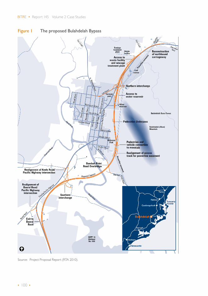
• 100 •


Figure 1 The proposed Bulahdelah Bypass

Source: Project Proposal Report (RTA 2010).

• 101 •


A brief history of the economic evaluation undertaken for the Bulahdelah Bypass is provided in this section with a detailed review of the RMS Contractor (2009) CBA analysis—the basis on which the decision was made to proceed with the project.

Ex-ante CBAsBefore the Federal Government’s decision to fund the Bulahdelah Bypass, there had been three CBAs looking into the project’s economic viability (table 1).

Table 1 Ex-ante CBAs for the Bulahdelah Bypass

MM/YY Cost estimate Benefit-cost ratio CBA author

11/2004 $153m (in 2003 prices) 3.5 (@7%) Parsons Brinckerhoff Australia (2004b)11/2007 $224m (in 2007 prices) 2.7 (@7%) Parsons Brinckerhoff Australia (2007b)08/2009 $304.5m (in 2009 prices) 2.1 (@7%) RMS Contractor (2009)

Source: Parsons Brinckerhoff (2004b and 2007b); RMS Contractor (2009).

The first CBA of the project was undertaken by Parsons Brinckerhoff in 2004 and reported in Technical Paper 13 of the Environmental Impact Statement (Parsons Brinckerhoff 2004b). The analysis was conducted following the NSW Government Guidelines for Economic Appraisal (NSW Treasury 1997) and the Economic Analysis Manual (RTA 1999 with 2002 update). Based on a capital cost $153m in 2003 prices, and a discount rate of 7%, the benefit-cost ratio (BCR) was estimated to be 3.5.

The second CBA was also undertaken by Parsons Brinckerhoff (2007b) (it was signed off by Parsons Brinckerhoff but the author was RMS Contractor) using a methodology similar to the one used in Parsons Brinckerhoff (2004b). Because of the higher project costs, the estimated BCR was lower (2.7 @7%).

The third (final) CBA was undertaken by RMS Contractor (2009), which updated the CBA prepared by Parsons Brinckerhoff in 2007. Like the earlier two studies, travel time savings were the main source of benefits (table 2). All three studies used identical methodology and modelling input for estimating travel time savings. As project costs increased, there was a further drop in the estimated BCR in RMS Contractor (2009) (2.1 @7%).

Since the RMS Contractor’ ex-ante CBA was the basis on which the final decision was made to proceed with the project, it was made the focus in our ex-post evaluation.

• 102 •


Table 2 Benefits and costs for the Bulahdelah Bypass (final ex-ante CBA) ($ millions)

Benefit/cost category @4% @7%

Discounted costs 306.8 288.0

Property 8.8 8.9Construction 279.8 269.0Rehabilitation 17.7 9.5Maintenance -0.6 -0.4Delays (caused by construction) 1.0 1.0Discounted benefits 979.5 611.0

Car VOC 41.7 26.0Truck VOC 5.3 2.0Car travel time 779.1 488.4Truck travel time 101.1 68.3Accidents 19.4 13.0Residual value 33.0 13.3NPV 672.7 323.0

BCR 3.2 2.1

FYRR (%) 9.4 8.7

1 Pacific Highway, Counting Station 09.909, Bulahdelah – South of Booral road (Parsons Brinckerhoff 2007a).

Source: RMS Contractor (2009).

Review of RMS Contractor (2009) analysisThe review of the RMS Contractor’ ex-ante CBA presented below concentrates on traffic demand forecasts and associated travel time modelling, and road user benefit estimation.

Traffic forecasts

The RMS Contractor (2009) study did not report traffic forecasts for the Pacific Highway at Bulahdelah in terms of annual average daily vehicles (AADV), but other sources (for example the Project Proposal Report (RTA 2010)) indicated a 4.3% a year (compound) growth up to 2008 and 2.45% a year (compound) for 2008-2028. These traffic forecasts were believed to come from the studies undertaken earlier by Parsons Brinckerhoff (2004a and 2007a), which were in turn based on the Pacific Highway Cumulative Impact Study (Scott Wilson Nairn Pty Ltd 1999).

At the time the final CBA was conducted, these traffic forecasts (prepared 10 years earlier) were judged to be still relevant, although there had already been an indication that traffic growth was slowing down (1.61%1 a year for 2001–2004 against the predicted average annual growth rate of 4.3% for 1999-2006 (both in compound terms)).

BITRE working paper 75 (BITRE 2009) forecast much lower growth:• Newcastle to Bulahdelah: 1.89% a year comprised of 2% for light vehicles and 1.09% for heavy

vehicles• Bulahdelah to Port Macquarie: 1.79% a year, comprised of 1.90% for light vehicles and 1.11% for

heavy vehicles.

Current data suggests that the traffic forecasts used for evaluating the Bulahdelah Bypass project were too optimistic.

• 103 •

Appendix B.3 • III Review of ex-ante CBAs

Traffic modelling

2 Efforts were made to locate this model, but without success.3 Another possible route is via Lee Street and Stroud Street, but this is longer and less practical.

The estimates of vehicle kilometres travelled (VKT) and vehicle hours travelled (VHT) used to calculate road user costs originated from a 2004 Parsons Brinckerhoff traffic study undertaken for an Environmental Impact Statement (EIS). Parsons Brinckerhoff (2004a) built a micro-scale travel demand model2 for the study area using the transport software suite “Transplan”. The model was built to test the impact on the road network’s operation from building the Bulahdelah Bypass. Table 3 shows Parsons Brinckerhoff ’s modelling results in terms of daily VKT, daily VHT and average speed.

Table 3 Traffic forecasts for the base case and project case

Year Base case

Project

Existing road Bypass Total

Daily vehicle kilometres of travel (VKT)

2008 152 450 6 848 130 103 136 9502018 193 710 8 727 165 813 174 5402028 246 130 10 606 201 514 212 120

% change pa

2008–18 2.42 2.45 2.45 2.462018–28 2.42 1.97 1.97 1.97

Daily vehicle hours of travel (VHT)

2008 3 020 136 1 304 1 4402018 5 300 173 1 667 1 8402028 9 320 210 2 060 2 270

% change pa

2008–18 5.79 2.44 2.49 2.482018–28 5.81 1.96 2.14 2.12

Average speed (km/h)

2008 50 50 100 952018 37 50 99 952028 26 50 98 93

Notes: % changes are calculated by BITRE.Source: RMS Contractor (2009). Original source is Parsons Brinckerhoff (2004a).

A number of anomalies can be found in table 3:• Daily VKT for the base case was modelled to be higher than the total for the project case

(by 11-16%) even though the project case route is longer than the base case route (8.5km versus 8.3km). Parsons Brinckerhoff (2004a) explained this result as traffic diversion to other roads in the base case due to the congestion along the old Pacific Highway. The extra distance travelled from diverting to alternate routes implied the length of the base case route was set to 9.5km for 2008 and 2018, and 9.9km for 2028. The site inspection undertaken by BITRE for this ex-post evaluation indicated that the most practical diversion route in the area was via Richmond and Stroud Streets,3 which is 8.4km long, well below the modelled length of the base case routes.

• 104 •


• Daily VKT was modelled to grow at similar rates for both the base and project cases for 2008–2018. However, for the next period, the modelled growth rate for the base case was higher at 2.4% a year compared with 2% a year for the project case. Growth in VKT is caused by traffic growth or increased travel distance. Since the same traffic growth was applied to both the base and project cases, the higher VKT growth for the base case must have been caused by further diversion from the old Pacific Highway.

• Similar patterns of growth apply for daily VHT, with the growth rate for the base case being even higher than the project case. Increased travel time due to congestion is believed to be responsible for this higher growth rate.

• The modelled average speeds for the base case routes appear to be very low. For example, the estimated average speed of 37km/h for the base case road in 2018 could be due to an assumed speed of 8km/h in the town centre4 (against a speed limit of 50 or 60km/h), and 49km/h for the approach road (against a speed limit of 80km/h). While this might be possible for holiday seasons or during peak hours, it is unlikely to be true for every hour of the day and every day of the year. Travel speed assumptions are critical to estimating travel time savings and they require a reassessment for this ex-post case study.

Road user benefit estimation

4 The length of the base case road in the town centre is assumed to be 2.4km with the approach road assumed to be 5.9km.

RMS Contractor (2009) used Excel spreadsheets to calculate the road user benefits of the project. The analysis followed the framework recommended by RTA’s Economic Analysis Manual (1999). However, its accuracy depends largely on the quality of work undertaken by Parsons Brinckerhoff (2004a) on traffic forecasts and travel speed modelling. Overly optimistic traffic forecasts and inaccurate travel speed modelling were likely to have caused the travel time savings to be grossly over estimated.

VOC savings were estimated using the speed-based VOC models in RTA (1999). These speed-based models assume a most efficient travel speed of approximately 50km for light vehicles and 70km for heavy vehicles. As speed decreases below or rises above these optimal speeds, unit VOCs increase. In the ex-ante CBA, unit VOCs of cars and trucks for the project case were generally higher than those for the base case because speeds were much higher than the optimal speeds. The estimated net savings in VOCs (table 2) were largely a result of the extra VKT modelled for the base case routes due to diversion.

Road user benefits beyond 2028 were assumed to remain at the year 2028 level, although this was not consistently executed due to spreadsheet errors in estimating travel time cost savings for trucks (figure 7) and the crash cost savings (figure 9).

• 105 •


Review of the ex-ante CBAs points to a need to update the traffic forecasts and travel time modelling.

Traffic demand analysisActual traffic data available up to 2013 indicate that there was a significant over-estimation of traffic demand for the Pacific Highway at Bulahdelah (figure 2). The initial (base year) traffic level was over 25% higher than the actual observed value. The traffic growth forecasts in the ex-ante analysis were also higher than those derived from the historical trend. Had the ex-ante CBA updated the Parsons Brinckerhoff ’s (2004a) forecasts using the then available information (for example, BITRE’s 2009 forecasts), the over-estimation could have been avoided.

Figure 2 Annual Average Daily Vehcles (AADV) at Bulahdelah: actual versus predicted (south of Booral Road)

Notes: Pacific Highway, Counting Station 09.909, Bulahdelah – South of Booral road.Source: Parsons Brinckerhoff (2004a); Project Proposal Report (RTA 2010); Wilkinson & Murray (2014) and BITRE (2009).

5000

10000

15000

20000

25000

30000

1958 1968 1978 1988 1998 2008 2018 2028 2038

0

Historical trend based on actual traffic counts

Actual traffic countsBITRE WP75Ex-ante

AA

DV

Year

• 106 •


A trend extrapolation method based on the historical data (10 actual observations between 1976 and 2013) was used to update the traffic forecasts for this ex-post evaluation. The updated traffic growth forecasts together with ex-ante estimates are presented in table 4. These forecasts are in broad agreement with the latest assessment by BITRE (2009) of the long-term trend of traffic growth in the area. For the ex-post study, a starting traffic level of 12,850 AADV in year 2010 (trend value, south of Booral Road) was used with an equivalent linear growth rate of 2.05% (2010 as the base).

Table 4 Traffic forecast compound growth rates (% a year)

Ex-ante Ex-post BITRE (2009)

2008–18 2.45 1.96 1.852018–28 1.97 1.64 1.852008–28 2.21 1.80 1.85

Source: Parsons Brinckerhoff (2004a) and BITRE (2009).

The traffic composition assumed in the ex-ante CBA of 20% heavy vehicles was close to observed values (Wilkinson & Murray 2014) and unchanged for the ex-post study.

The ex-ante CBA over-estimated the traffic on the bypass due to two errors made in the estimation. First, the traffic modelling results from Parsons Brinkerhoff (2004a) included both local and through traffic, but RMS Contractor (2009) treated local traffic as if it was through traffic. According to Parsons Brinkerhoff (2004a), local traffic accounted for approximately 8–10% of total traffic in Bulahdelah. Second, it was arbitrarily assumed that 95% of the total traffic would use the bypass. The actual bypass traffic was 87% of through traffic—observed during the week from 28 November to 4 December 2013 (Wilkinson & Murray 2014). These two errors had the effect of placing local traffic on the bypass road and also over-estimating the amount of through traffic that would use the bypass.

Road user cost estimationTravel time cost savings accounted for over 91% of the total estimated road user benefits in the ex-ante CBA. The key task for this ex-post evaluation was to update the travel time modelling, the results of which are critical for accurate estimation of travel time cost savings. Another task was to re-estimate VOC savings by altering the assumption about the length of the base case road and choosing more appropriate unit VOC values.

Travel time modellingWithout having had access to the original traffic model, an alternative approach was developed which involved the following steps: • developing a simplified road network consisting of a synthetic base case road and the town

bypass road only • estimating travel speed on the existing road and the newly built bypass for each of the major

categories of hourly volume distribution for traffic • deriving average daily travel speeds for use in estimating VKT and VHT in the ex-ante CBA

spreadsheet model.

• 107 •


Simplified bypass network

Bulahdelah is a small town with a very simple road network. The old Pacific Highway is the primary arterial road that traverses north-south through the town. Other major roads connecting to the town provide links to the regional locations of: • Gloucester via Stroud Street and Markwell Road• Forster via The Lakes Way • Stroud via Booral Road and The Bucketts Way.

Local roads in the town generally run north-south and east-west in a grid pattern, as shown in figure 1. Stroud Street, used as the old highway at one time and considered to be the town’s main street, provides access to the retail and commercial centre, and the industrial areas to the north. There are two signalised pedestrian crossings on the old Pacific Highway, one to the south of Blanch Street and the other to the north of Stuart Street. As traffic at Bulahdelah was dominated by through traffic on the Pacific Highway before the bypass was completed, the road network in the study area can be simplified by only evaluating the benefits to through traffic without losing too much validity. Figure 3 is a schematic diagram of the existing and bypass roads at Bulahdelah.

Figure 3 Schematic diagram of the existing and bypass roads at Bulahdelah

Section 1 Northern ApproachSpeed limit: 80km/h

Section 2 Northern built-up areaSpeed limit: 60km/hLength: 0.75km

Section 4 Southern built-up areaSpeed limit: 60km/hLength: 0.4km

Section 5 Southern ApproachSpeed limit: 80km/h

Section 3a Diversion route via Stroud/Richmond StreetSpeed limit: 50km/hLength: 1.4km

Section 3b Old Pacific HighwaySpeed limit: 60km/hLength: 1.25km

Tow

n By

pass

(pro

ject

) Sp

eed

limit:

110

km/h

Leng

th: 8

.5km

Base

cas

e To

wn

Cen

tre

rout

esLe

ngth

: S2+

S4+

(S3a

+S3

b)/2

=2.

5km

• 108 •


A number of key characteristics of the simplified Bulahdelah road network are summarised below:

5 Total reported length of the base case road.

• The length of the base case town centre route is 2.5km (sum of sections 2 and 4 plus the average length of sections 3a and 3b). Sections 3a and 3b are the two main alternative town centre routes. Section 3b (the old Pacific Highway) is shorter and has a higher speed limit (60km/h), but with two traffic lights for pedestrian crossings, a service station and a sharp curve section with a recommended speed of 40km/h. Section 3a (via Stroud and Richmond Streets) runs through the town centre, is longer and has a lower speed limit (50km/h), but without any traffic lights. Sections 2 and 4 are built-up areas next to the town centre with a 60km/h speed limit. They are included in the total length of the base case town centre routes to allow for any queuing that might occur in busy and holiday periods.

• The total length of the approach road in the base case is 5.9km (8.3km5 – 2.4km (sections 2, 3b and 4)) with a speed limit of 80km/h. In the project case, traffic travelling to or going through the town centre has the option to travel on part of the newly built bypass, notably at the southern end (figure 1). Higher travel speed on the bypass results in a higher average speed for traffic travelling on the approach road. This average speed is calculated as the length-weighted average of the speed limits for the old and new roads. Of the 5.9km of approach road, 1.2km remains at the old 80km/h speed limit while the remaining 4.7km changes to 110km/h giving an average speed of 104km/h.

• The total length of the bypass is 8.5km with a speed limit of 110km/h. • Traffic levels may vary across the different sections of the base case road, but the recent data

from Wilkinson & Murray (2014) shows that traffic volumes north and south of the bypass are similar (close to 14,500 vehicles a day) and 87% of this traffic uses the bypass with the remainder staying on the base case town centre routes.

• Base case traffic in Bulahdelah was assumed to comprise 90% through traffic and 10% local town traffic. Local traffic was included in the traffic within the town centre to estimate the level of congestion for both the base and project cases. However, no benefits were calculated for the local traffic, which would lead to a slight under-estimation of total road user benefits.

Travel speed estimation

In the ex-ante traffic study (Parsons Brinckerhoff 2004a), travel speed was modelled on the basis of 13% of AADV in the 100th-highest hour. The current traffic update aims to model travel speed for each of the major categories of the hourly flow distribution. This is consistent with the approach recommended by Austroads (2003).

A traffic flow histogram specific to the project site was not available. Two alternatives were considered: default values sourced from RTA (2000) for the National Highway in NSW and an hourly flow distribution for the nearby town Nabiac.

Table 5 compares these two alternatives. It shows that the hourly flow distribution for Nabiac contains more heavily trafficked hours than the state average—an extra 459 hours a year for the total of categories higher than 8% of AADT.

• 109 •


Table 5 Hourly flow distributions for National Highways in NSW and Nabiac

Hours a year (8,760)

Hourly Traffic Flow Categories (% of AADT)

0<Flow≤4 4<Flow≤8 8<Flow≤12 12<Flow≤16 Flow>16

National Highway in NSW 4,647 3,487 619 7 0Nabiac 4,665 3,010 971 96 18

6 Refer to Austroads (2005).

Source: Austroads (2003) and Nabiac hourly traffic count data from RMS (2015).

Congestion in peak hours and long traffic queues recorded by RMS traffic counters at Bulahdelah before the bypass had been built led to the conclusion that the estimated hourly flow distribution for Nabiac was a better representation of the traffic pattern at Bulahdelah. Use of Nabiac data also allowed travel speed to be modelled more accurately using more disaggregated hourly flow volumes as shown in figure 4.

Figure 4 Nabiac hourly flow histogram 2014–15

In estimating the travel speeds for each of the hourly traffic flow categories listed in figure 4, a range of assumptions were made:• The model road state (MRS)6 for the base case road was assumed to be 11 with a capacity of

2,500 passenger car equivalent units per hour (PCE/h). The MRS for the newly-built bypass was classified as 21 with a capacity of 8,000 PCE/h.

• To determine the volume-capacity ratios (VCRs) for each hourly flow category, PCE units were required. Using the Austroads (2005) conversion factors and the observed traffic composition from the Nabiac hourly traffic count data, the aggregate AADV to PCE conversion factor was calculated to be 1.26 and applied to estimate VCRs for each hourly flow category.

• The base case road was characterised as ‘curvy’ and the project case road as ‘straight’.

0

500

1 000

1 500

2 000

2 500

3 000

3 500

Hourly Flow (% of AADT)

>20%18-20%16-18%14-16%12-14%10-12%8-10%6-8%4-6%2-4%0-2%

Hou

rs p

er y

ear

3 249

1 4161 277

1 733

788

18378 18 14 3 1

• 110 •


• The speed limit for the synthetic base case town centre routes was set to 55km/hour (based on the average speed limit of Sections 3a and 3b). The combined capacity of the parallel Sections 3a and 3b was assumed to be 2,500 PCE/h. These assumptions are all on the conservative side to avoid over-estimating travel speeds for the base case.

• The speed limit for the base case approach road was set to 80km/h. • The congested speed for the bypass road was set at 30km/h according to the Austroads

recommended speed-flow curve for rural areas, and that for the base case town centre routes to 7.8km/h. The latter assumption was intended to allow for effects of intersections and traffic lights in the town centre that would be similar to an urban environment. A modified7 urban Akcelik speed-flow curve (Austroads 2011) was adopted for the town centre routes (figure 5). Half of the length of the approach road (sections 1 and 5) was subject to a congested speed of 7.8km/hr to represent queues extending out of the town while the other half was set to 30km/hr similar to the bypass road. This was to reflect typical traffic behaviour heading into and out of a town centre.

• Articulated trucks were used to estimate the average speed of trucks.

7 The lower limit to congested speed for the Akcelik speed curve was set to 7.8km/h for VCR > 1.25.

Figure 5 Akcelik urban speed-flow curve with lower speed limited to 7.8km/h

Source: Based on Austroads (2003a).

Updated results on travel speed

For comparison purposes, the same traffic values as in the ex-ante analysis were used to estimate traffic flow and volume-capacity ratios for each of the hourly flow distribution categories. The calculated volume-capacity ratios were then used to determine travel speeds through the assumed speed-flow curves. Table 6 updates average daily travel speed estimates for both the

0

0.0 1.501.401.301.201.101.000.900.800.700.600.500.400.300.200.10

10

20

30

40

50

60

70

Volume-capacity ratio

Spee

d (k

m/h

)

• 111 •


base case and project case roads. As seen, the ex-ante travel speed estimates for the base case were significantly lower than the updated speed estimates. The speed estimates in the ex-ante analysis were likely to be associated with the speeds for peak periods experienced in the town.8

Table 6 Update of travel speed estimates (km/h) – original traffic forecasts

Year

Base case (km/h) Project case (km/h)

Approaches Town centre Averagea Approaches Town centre Average Bypass

Ex-ante

2008 50 50 1002018 37 50 992028 26 50 98

Ex-post (based on original traffic forecasts)

2008 72 50 66 104 55 89 1092018 67 45 61 104 55 89 1092028 61 38 54 104 55 89 108

8 No information was found on the expansion factor from the ex-ante traffic study (Parsons Brinckerhoff (2004a) nor from the ex-ante CBA (RMS Contractor 2009).

9 Seal road with NRM less than 50.

a Weighted by section length.

As for the project case, travel speeds on the town site route were significantly under-estimated by the ex-ante study. This is because it wasn’t anticipated that part of the bypass road could be used by traffic travelling through the townsite route under the project case.

The travel speed estimates reported in table 6 are based on the original traffic forecasts used in the ex-ante CBA. A lower actual traffic level for the base year and lower forecast traffic growth for future years at Bulahdelah mean that predicted travel speeds for the base case of the ex-post analysis are even higher (table 7).

Table 7 Update of travel speed estimates (km/h) – updated traffic forecasts

Base case (km/h) Project case (km/h)

Year Approaches Town centre Averagea Approaches Town centre Average Bypass

2008 74 52 68 104 55 89 1092028 73 50 66 104 55 89 1092028 71 46 64 104 55 89 109

a Weighted by section length.

Vehicle operating cost estimation

In the ex-ante CBA, the forecast VKT from traffic modelling and unit vehicle operating costs were used to estimate changes in vehicle operating costs (VOCs). The unit costs for the base case and the existing road for the project case were derived from the urban stop-start model in the RTA Economic Analysis Manual, which relates VOC to speed of travel. The unit VOCs for cars and trucks using the bypass were also assumed to vary with speed. These unit costs were sourced from the RTA VOC look-up tables for rural roads of base grade, base curvature and very good seal surfaces (S5)9.

Two problems were found in the estimation of VOC savings/dis-savings. First, the base case town site route was not in a typical stop-start condition for all the sections and for all time. While the

• 112 •


stop-start condition might apply in the most congested hours such as peak holiday seasons in the vicinity of the town centre, it would be not suitable for most other times and for the approach road which had half of the total length of the base case road. Applying a stop-start model for the entire length and for all periods over-estimates the VOCs for the base case and hence the project’s VOC savings.

Second, the urban stop-start model used by RMS Contractor (2009) took the form:

10 Had the data permitted, aggregation could have been done using more detailed vehicle categories, which would have produced better estimates of unit VOCs for heavy vehicles.

c = A + B/V

where: c= VOC (cents/km); V= journey speed (km/h); and A and B are model coefficients. RMS Contractor (2009) used the coefficients (A and B) for rigid trucks to represent those for the entire “heavy vehicles” category. This resulted in an under-estimation of the unit VOC for the base case.

In the ex-post evaluation, both errors were corrected. As discussed earlier, the congested speed for the approach road was assumed to be 30km/hour rather than 7.8km/hour. Unit VOCs for heavy vehicles were represented by a weighted average of the unit VOCs for rigid and articulated trucks.10 Table 8 presents unit VOC values for both ex-ante and ex-post analyses. It is worth noting that, unlike the ex-ante analysis, unit VOC values for trucks for the base case in the ex-post evaluation were estimated to be higher than those for the project case. This result is considered to be more intuitive—trucks travelling at 110km/h on the bypass would be more efficient than travelling at a stop-start speed of less than 50 or 60km/h through the town centre routes.

Table 8 Unit VOC values for ex-ante and ex-post analyses (cents/km)

Ex-ante Ex-post (corrected)

Base Project Base Project

Existing Bypass Existing Bypass

Car 2008 28.97 28.97 29.95 30.14 30.05 30.242018 29.74 28.97 29.95 30.18 30.05 30.242028 30.81 28.97 29.95 30.25 30.05 30.23

Truck 2008 83.94 83.94 101.75 112.22 111.56 104.762018 87.77 83.94 101.75 112.52 111.56 104.752028 93.10 83.94 101.75 113.01 111.57 104.74

The savings in VOCs reported in the ex-ante CBA were largely caused by the increased VKT in the base case due to the modelled diversion from the Old Pacific Highway to other longer routes. This anomaly was corrected in the ex-post CBA by applying a series of adjustment factors to the VKT based on the assumed (or modelled) length of the base case road over time (table 9). The average length (8.4km) recommended for the ex-post analysis was based on the average length of the Old Pacific Highway and the diversion route through Richmond/Stroud Street. In the ex-ante traffic study, the modelled length increases over time as congestion causes more traffic to divert to longer routes.

• 113 •


Table 9 Adjustment of the length of the base case road (km)

Ex-ante Ex-post Adjustment factor

2008 9.5 8.4 0.892018 9.4 8.4 0.892028 9.9 8.4 0.85

Crash analysisNo crash rate was explicitly reported in the ex-ante CBA. There was only a reference to the traffic report by Parsons Brinckerhoff (2004a) that stated it was higher than the state average. The traffic report claimed that the average crash rate over the 12-year period from 1990 to 2001 for the town road was 99.6 crashes per 100 million vehicle kilometres travelled (MVKT), twice the state average for a rural two-lane undivided road (49.3 crashes per 100 MVKT). The report contained insufficient information to replicate the 99.6 per 100 MVKT average crash rate.

In reviewing the ex-ante crash analysis, the crash rate was re-calculated using the crash numbers (all crashes, including property damage only) for each year provided in the traffic report, the section length of 8.4km and estimated traffic readings for those years (RTA 2000). These numbers and the resulting crash rates are shown in table 10 and plotted in figure 6. As seen, the crash rate fluctuated between 28.2 and 70.7 crashes per 100 MVKT with an average of 47.5 crashes per 100 MVKT.

Table 10 Crash rates for the base case road (1990–2001)

Year Estimated AADV MVKT Accidents Crash rate (crashes/100 MVKT)

1990 7 578 23.2 13 56.01991 7 842 24.0 14 58.21992 8 105 24.9 7 28.21993 8 369 25.7 10 39.01994 8 633 26.5 11 41.61995 8 896 27.3 10 36.71996 9 160 28.1 10 35.61997 9 424 28.9 18 62.31998 9 687 29.7 21 70.71999 9 951 30.5 21 68.82000 10 215 31.3 12 38.32001 10 478 32.1 11 34.2

Source: AADV (RTA 2001), MVKT (based on an 8.4km section length), Accident numbers (Parsons Brinckerhoff 2004a)

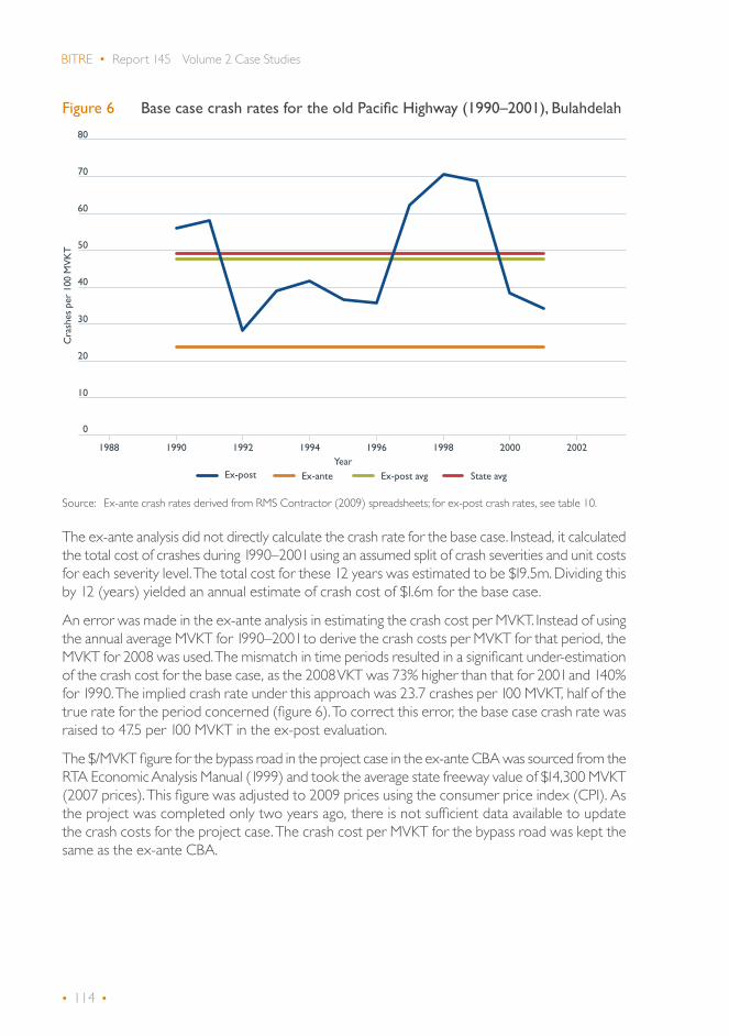
• 114 •


Figure 6 Base case crash rates for the old Pacific Highway (1990–2001), Bulahdelah

Source: Ex-ante crash rates derived from RMS Contractor (2009) spreadsheets; for ex-post crash rates, see table 10.

The ex-ante analysis did not directly calculate the crash rate for the base case. Instead, it calculated the total cost of crashes during 1990–2001 using an assumed split of crash severities and unit costs for each severity level. The total cost for these 12 years was estimated to be $19.5m. Dividing this by 12 (years) yielded an annual estimate of crash cost of $1.6m for the base case.

An error was made in the ex-ante analysis in estimating the crash cost per MVKT. Instead of using the annual average MVKT for 1990–2001 to derive the crash costs per MVKT for that period, the MVKT for 2008 was used. The mismatch in time periods resulted in a significant under-estimation of the crash cost for the base case, as the 2008 VKT was 73% higher than that for 2001 and 140% for 1990. The implied crash rate under this approach was 23.7 crashes per 100 MVKT, half of the true rate for the period concerned (figure 6). To correct this error, the base case crash rate was raised to 47.5 per 100 MVKT in the ex-post evaluation.

The $/MVKT figure for the bypass road in the project case in the ex-ante CBA was sourced from the RTA Economic Analysis Manual (1999) and took the average state freeway value of $14,300 MVKT (2007 prices). This figure was adjusted to 2009 prices using the consumer price index (CPI). As the project was completed only two years ago, there is not sufficient data available to update the crash costs for the project case. The crash cost per MVKT for the bypass road was kept the same as the ex-ante CBA.

0

10

20

30

40

50

60

70

80

State avgEx-post avgEx-anteEx-post

1988 20021990 1992 1994 1996Year

1998 2000

Cra

shes

per

100

MV

KT

• 115 •


Project costsThe project was budgeted to cost $379 million outturn as noted in the February 2010 Project Proposal Report ($360m in 2009 prices). In the ex-ante CBA, expended costs ($59m in 2009 prices) were excluded from the economic appraisal leading to a total estimated outturn cost of $304.5 million (2009 prices). Costs that are already expended are present in both the base and project cases and usually ignored when conducting CBA as they are not relevant to the investment decision (ATC 200611). Unlike the ex-ante CBA, the ex-post CBA included all the costs related to this project. This would provide a better measure of the economic viability of the project.

Information on actual project costs was sourced from the Post Completion Review report (RMS 2013). The final outturn cost was reported as $315 million (including the costs classified as expended in the ex-ante study). Using CPI as a deflator, the final project cost was estimated to be $297.5 million in 2009 prices (table 11).

Table 11 Property and construction cost flows ($m, in 2009 prices)

Year

Ex-ante Ex-post

Land Construction Total Land Construction Total

2009 3.4 – 3.4 3.4 56.0 59.42010 5.3 54.7 60.0 5.3 17.0 22.32011 90.0 90.0 89.0 89.02012 120.0 120.0 87.9 87.92013 31.1 31.1 38.9 38.9Total 304.5 297.5

Residual valuesResidual values (RV) capture the remaining benefits that the project may offer beyond the evaluation period. The ex-ante CBA estimated the RV using the component method. This method estimates the RV as the sum of the remaining values after straight line depreciation is applied to infrastructure components in the project with differing lives and costs for the evaluation period.

The formula used in the ex-ante CBA to estimate the residual value was: n

Residual value (Component) = A +∑Capital costsi ×Asset lifei − Evaluation period

Asset lifei

i=1

where:

11 According to ATC (2006, Volume 3, page 55, footnote 1), “Leave out any planning and investigation costs already incurred at the time of undertaking the BCA. The decision about whether or not to proceed with the initiative will have no effect on these costs.”

n = total number of infrastructure componentsa = total cost of all non-depreciable components ($)Capital costsi= cost of component i ($)Asset lifei= estimated life of component i (years)Evaluation period = usually 30 years in Australia.

• 116 •


Table 12 reproduces the RV estimates using the component approach adopted in the ex-ante analysis.

Table 12 Ex-ante residual value calculation – component method

Infrastructure Cost ($’000) Assumed Life (years)

Remaining life (years)

% remaining Residual value ($’000)

Earthworks 96 731 40 10 25 24 183Drainage 24 679 40 10 25 6 170Pavements – concrete 32 005 40 10 25 8 001Pavements – flexible 18 440 20 –10 50* 9 220Structures 80 655 100 70 70 56 459Other construction 21 252 20 –10 50* 10 626Refurbish old route 2 318 20 –10 50* 1 159Total 115,817

* Assumes that assets are replaced during maintenance once their assumed life is exhausted, and their life is renewed for the same number of years at the same initial cost.

Source: RMS Contractor (2009).

Property that was acquired by the project totalling $8.1m was not included in the residual value in the ex-ante CBA. Land that has been included as an investment cost and that can be sold for an alternative use at the end of the project’s life can be accorded a residual value as stated in Volume 5 of the National Guidelines to Transport System Management (ATC 2006). In this ex-post evaluation, land was included in the RV estimation using the component method, bringing the total residual value to $123.9m.

Four alternative RV estimation methods were used in a sensitivity analysis. These were:• straight-line depreciation (SLD)• decreasing net benefits (DNB)• constant net benefits (CNB) • increasing net benefits (INB).

For a detailed description of each of these, see appendix E of the main report.

Estimation of RVs using the SLD method requires an assumption about the length of asset life. Different components of the project have different lifespans with different costs. It was assumed that the average lifespan of the bypass is 50 years. This was based on previous estimates of 40 to 60 years as the economic life of road projects (QDTMR 2011, TfNSW 2013 and Austroads 2003b). Calculating the cost-weighted average life of the project using the estimated life of different asset types yields 54.5 years, close to the 50-year estimate (table 13).

• 117 •


Table 13 Asset life estimation

Infrastructure components Cost ($’000) Estimated life (years) Weighted average life (years)

Property 8 100 Indefinite N/AEarthworks 96 731 40 14.0Drainage 24 679 40 3.6Pavements – concrete 32 005 40 4.6Pavements – flexible 18 440 20 1.3Structures 80 655 100 29.2Other construction 21 252 20 1.5Refurbish old route 2 318 20 0.2

Total weighted project life (years) 54.5

Source: RMS Contractor Pty Ltd (2009).

Base and price yearThe price year is 2009 and the base year is 2010, the same as the ex-ante CBA.

Discount rateThe ex-ante CBA conducted the main assessment at 7% with sensitivity tests at 4% and 10%. The ex-post CBA is under taken with a 4% discount rate with a sensitivity test at 7%. This is consistent with the approach currently favoured by the Commonwealth Department of Infrastructure, Regional Development and Cities.

• 119 •


Thanks to RMS’s records, the ex-ante CBA was replicated without difficulty. However, due to the lack of original traffic model, estimates of VKT, VHT and travel speeds could not be replicated.

• 121 •


A number of adjustments were made to the ex-ante CBA:E1. Revising travel speed, section length and unit VOC estimatesE2. Updating project costsE3. Updating traffic forecastsE4. Correcting errors in safety benefit estimationE5. Updating RV estimates.

A sensitivity analysis was also undertaken with respect to the discount rate.

Revising travel speed, section length and unit VOC estimates (E1)Three revisions were made in the first set of adjustments (E1): 1. an increase of travel speed for the base case and project case roads as shown in table 62. a reduction of the length of the base case road (table 9), and 3. an adjustment of unit VOC values based on the revised speed estimates and changed

coefficients in the VOC prediction model for trucks in the urban environment (table 8).

Changing the travel speed assumption had impacts on travel time and VOC saving estimates. The increased travel speed for the base case led to a significant reduction in travel time cost (TTC) savings (-68% for cars and -42% for trucks) (table 14).

Table 14 Revising travel speed, section length and VOC unit costs (E1)

@4% discount rate ($m, in 2009 prices) Ex-ante E1 E1/Ex-ante (%)


Construction costs 279.8 279.8 0.0Property costs 8.8 8.8 0.0Maintenance costs -0.6 -0.6 0.0Rehabilitation costs 17.7 17.7 0.0Delay costs 1.0 1.0 0.0Discounted benefits 979.5 380.2 –61.2

Car TTC savings 779.1 252.6 –67.6Truck TTC savings 101.1 59.0 –41.6Car VOC savings 41.7 0.0 –100.0Truck VOC savings 5.3 19.4 265.8

Continued…

• 122 •



Accident savings 19.4 16.3 –16.3Residual value 33.0 33.0 0.0Net present value (NPV) 672.7 73.4 –89.1

Benefit–cost ratio (BCR) 3.19 1.24

First-year rate of return (FYRR) 9.4% 4.2%

Reducing the length of the base case road and changing assumptions about unit VOCs for the base and project cases had offsetting effects. Downward adjustment of the base case section length alone would lead to reductions in VOC savings for both car and trucks. Changing the unit VOC assumptions for trucks more than offset the reduction in VOC savings caused by shortening the base case road length. Similar unit VOCs for cars in the ex-post CBA for both base and project cases means there are no VOC savings for cars. The overall reduction in VOC savings for cars and trucks was 59%.

As a result of reduction in the length of the base case road, safety benefits fell by 16.3%.

Adjustments made in E1 removed 89% of the positive net present value estimated in the ex-ante CBA. The estimated BCR dropped from 3.19 to 1.24.

Updating projects costs (E2)The total cost for construction and property in the ex-ante CBA was estimated to be $304.5m (excluding expended costs). The actual cost in 2009 prices was estimated to be $297m (including expended costs). As expected, the discounted construction costs in E2 were only slightly lower than those in E1 (–1.3%, table 15) and as a result, the change to the BCR was minimal.

Table 15 Correction to project costs (E2)



Construction costs 279.8 276.2 -1.3Property costs 8.8 8.8 0.0Maintenance costs -0.6 -0.6 0.0Rehabilitation costs 17.7 17.7 0.0Delay costs 1.0 1.0 0.0Discounted benefits 380.2 380.2 0.0

Car TTC savings 252.6 252.6 0.0Truck TTC savings 59.0 59.0 0.0Car VOC savings 0.0 0.0 0.0Truck VOC savings 19.4 19.4 0.0Accident savings 16.3 16.3 0.0Residual value 33.0 33.0 0.0Net present value (NPV) 73.4 77.0 5.0



• 123 •


Updating traffic forecasts (E3)Updating the traffic forecast comprised three elements:1. base year through traffic volumes were revised down from 17,000 to 12,850 vehicles per

day (–24%),2. the forecast traffic growth was revised down as shown in table 4, and3. the split in through traffic between the existing and bypass roads was changed from 5:95

to 13:87.

Lower base year traffic volumes, growth forecasts and use of the bypass resulted in a fall in the total road user benefits (–43.4%). The NPV became negative with the BCR dropping to 0.71 (table 16).

Table 16 Updating traffic forecasts (E3)

@4% discount rate ($m, in 2009 prices) E2 E3 E3/E2 (%)


Construction costs 276.2 276.2 0.0Property costs 8.8 8.8 0.0Maintenance costs -0.6 -0.6 0.0Rehabilitation costs 17.7 17.7 0.0Delay costs 1.0 1.0 0.0Discounted benefits 380.2 215.3 –43.4

Car TTC savings 252.6 132.3 –47.6Truck TTC savings 59.0 30.9 –47.6Car VOC savings 0.0 -1.8 naTruck VOC savings 19.4 10.3 –47.0Accident savings 16.3 10.6 -34.6Residual value 33.0 33.0 0.0Net present value (NPV) 77.0 -87.9 –214.2



The effect of the traffic update on travel time savings can be better appreciated if compared with the E1 correction. Figure 8 shows the impact of the traffic update on annual TTC savings—the upper part for cars and the lower part for trucks. As seen, the E3 update almost halved the TTC savings for both cars and trucks associated with E1.

The sharp fall in ex-ante TTC savings for 2029 in figure 7 is due to a spreadsheet error. The over-estimation of TTC savings in the ex-ante CBA would have been greater had the error not been made. In the ex-ante study, it was assumed that road user benefits for year 2029 and beyond would remain at the level in 2028.

Figure 8 shows a similar over-estimation of car VOC savings, which become negligible following the E1 and E3 corrections. Compared with E3, truck VOC savings were under-estimated in the ex-ante analysis, notably for the early years of the evaluation period.

• 124 •


Figure 7 TTC savings for ex-ante analysis, E1 and E3 updates

Cars

Trucks

2010 2015 2020 2025 2030 2035 2040 2045Year

0

10

20

30

40

50

60

70

80

E3 - CarE1 - CarEA - Car

Car

TT

C s

avin

gs ($

m)

2010 2015 2020 2025 2030 2035 2040 2045Year

0

2

4

6

8

10

12

14

E3 - TruckE1 - TruckEA - Truck

Truc

k T

TC

sav

ings

($m

)

• 125 •


Figure 8 VOC savings for ex-ante analysis, E1 and E3 updates

Cars

Trucks

2010 2015 2020 2025 2030 2035 2040 2045

-1.0

-0.5

0.0

0.5

1.0

1.5

2.0

2.5

3.0

3.5

4.0

YearE3 - CarE1 - CarEA - Car

Car

VO

C s

avin

gs ($

m)

2010 2015 2020 2025 2030 2035 2040 2045

-1.0

-0.5

0.0

0.5

1.0

1.5

2.0

YearE3 - TruckE1 - TruckEA - Truck

Truc

k VO

C s

avin

gs ($

m)

• 126 •


Correcting errors in safety benefit estimation (E4)Accident cost savings were under-estimated in the ex-ante CBA due to the low crash rate used for the base case. This error was corrected by increasing the base case crash rate from 23.7 to 47.5 crashes per 100 MVKT (figure 6). This crash rate could be further updated if more recent data prior to the completion of the project were to become available.

Correcting the error in the base case crash rate almost tripled the accident cost savings and contributed an additional $20m in benefits (table 17). This update improved the BCR slightly bringing it from 0.71 to 0.78.

Table 17 Revising the base case crash rate (E4)



Construction costs 276.2 276.2 0.0Property costs 8.8 8.8 0.0Maintenance costs -0.6 -0.6 0.0Rehabilitation costs 17.7 17.7 0.0Delay costs 1.0 1.0 0.0Discounted benefits 215.3 235.9 9.6

Car TTC savings 132.3 132.3 0.0Truck TTC savings 30.9 30.9 0.0Car VOC savings -1.8 -1.8 0.0Truck VOC savings 10.3 10.3 0.0Accident savings 10.6 31.2 193.9Residual value 33.0 33.0 0.0Net Present value (NPV -87.9 -67.3 –20.6



Figure 9 compares the accident cost savings between the ex-ante analysis and the various updates. The accident savings in the ex-ante analysis totalled $19.4m (table 14) and also, for two years, the savings were incorrectly set to zero (2041 and 2042). The corrected safety benefit, at $31.2m, is 61% higher than the ex-ante estimate.

• 127 •


Figure 9 Accident cost saving estimates for ex-ante CBA and E1, E3 and E4 updates

Revising the RV estimate (E5)The ex-ante BCA did not include the land in the residual value. The correction here adds it in. A sensitivity analysis was conducted using alternative methods to calculate the RV. The results are presented in table 18.

As expected, adding the value of land improved the RV estimate slightly (by $2m), causing a marginal improvement in BCR (from 0.78 in E4 to 0.79 in E5). The SLD approach produced results similar to those derived from the component method. The RV estimates based on the net benefit approach varied extensively, ranging from 14% to 29% as a share of total discounted benefits.

Table 18 RV update and sensitivity test with alternative estimation methods (E5)

@4% discount rate ($m, in 2009 prices)

E4 Residual values

Component approach (ex-ante)

Component approach (ex-post)

RV1(SLD) RV2(DNB) RV3(CNB) RV4(INB)

Discounted costs 303.2 303.2 303.2 303.2 303.2 303.2

Capital costs 276.2 276.2 276.2 276.2 276.2 276.2Property costs 8.8 8.8 8.8 8.8 8.8 8.8Maintenance costs -0.6 -0.6 -0.6 -0.6 -0.6 -0.6Rehabilitation costs 17.7 17.7 17.7 17.7 17.7 17.7Delay costs 1.0 1.0 1.0 1.0 1.0 1.0Discounted benefits 235.9 236.7 238.2 240.1 271.9 284.9

Car TTC savings 132.3 132.3 132.3 132.3 132.3 132.3Truck TTC savings 30.9 30.9 30.9 30.9 30.9 30.9

Continued…

2010 2015 2020 2025 2030 2035 2040 2045Year

0.0

0.5

1.0

1.5

2.0

2.5

3.0

E4E3E1 EA

$m

• 128 •



E4 Residual values

Component approach (ex-ante)

Component approach (ex-post)

RV1(SLD) RV2(DNB) RV3(CNB) RV4(INB)

Car VOC savings –1.8 –1.8 –1.8 –1.8 –1.8 –1.8Truck VOC savings 10.3 10.3 10.3 10.3 10.3 10.3Accident savings 31.2 31.2 31.2 31.2 31.2 31.2Residual value 33.0 33.9 35.3 37.3 69.0 82.1

(RV as % of total benefits)

14.0% 14.3% 14.8% 15.5% 25.4% 28.8%

Net present value (NPV) –67.3 –66.5 –65.0 –63.1 –31.3 –18.3

Benefit–cost ratio (BCR) 0.78 0.78 0.79 0.79 0.90 0.94

Change in the discount rate (E6)Increasing the discount rate from 4% to 7% reduced the estimated BCR from 0.79 to 0.51 (table 19). The discounted project costs were largely unaffected, but the discounted benefits fell sharply (–39%). The impact of changing the discount rate is most apparent in the RV estimate that was subject to greater discounting due to its place in the far future.

Table 19 Change in the discount rate (E6)


Discounted costs 303.2 287.2 -5.3%

Construction costs 276.2 268.1 -2.9%Property costs 8.8 8.9 1.1%Maintenance costs -0.6 -0.4 -32.2%Rehabilitation costs 17.7 9.5 -46.5%Delay costs 1.0 1.0 -3.4%Discounted benefits 238.2 145.7 -38.8%

Car TTC savings 132.3 85.6 -35.3%Truck TTC savings 30.9 20.0 -35.3%Car VOC savings –1.8 –1.2 -32.7%Truck VOC savings 10.3 6.7 -35.1%Accident savings 31.2 20.4 -34.6%Residual value 35.3 14.2 -59.7Net Present value (NPV) –65.0 –141.5 117.6%


First-Year Rate of Return (FYRR) 2.9% 2.8%

• 129 •


SummaryTo bring together the ex-post evaluation results, the components of the total variation in NPV between the ex-ante and ex-post analysis are set out in figure 10. The ex-post NPV was estimated to be –$65.0m, which is $738m lower than the ex-ante estimate. The BCR fell from 3.19 to 0.79 making the project economically unviable.

Errors made in the ex-ante CBA in relation to travel speed, section length and unit VOC (E1) were the largest source of over-estimation of the NPV, contributing 81% (or –$599m) to the difference between the ex-ante and ex-post results. The second largest source of variation was the traffic update (E3), which reduced the NPV by a further $165m. Other adjustments, namely the project cost update (E2), improved methodology for safety benefit estimation (E4) and RV (E5), contributed positively to the gap in NPV between the ex-ante and ex-post analysis, but only marginally.

Sensitivity tests with respect to the RV showed that estimates based on the different methods of projecting the benefit stream into the future varied significantly (ranging between 14–29% as a share of total discounted benefits). However, even with the highest possible RV assumed, the project remains economically unviable. As expected, increasing the discount rate from 4% to 7% led to a lower BCR (0.51).


To check the plausibility of the estimates for this ex-post evaluation, this study compared the Bulahdelah bypass project with other national road bypass projects. The comparison is shown in table 20.

-700.0

-600.0

-500.0

-400.0

-300.0

-200.0

-100.0

0.0

100.0

$m


E3-E4(Accident)

E2-E3(Traffic)

E1-E2 (Cost)

EA-E1 (Speed, Length, VOC)

-599.3

3.6

-164.9

20.602.30

Ex-ante NPV = $672.7mEx-post NPV = –$65.0m

• 130 •


While it is difficult to find a project with similar characteristics for comparison, it is possible to compare the Bulahdelah bypass project with other recently completed projects on the basis of certain parameters, for example, size of the population of the bypass town, base year traffic level or project costs. • On a population basis, two projects are relevant for comparison: the Holbrook and Nagambie

bypasses. However, traffic levels were much lower in these two towns. Offsetting this were lower project costs on a $/km basis. Assuming that the ex-ante BCRs for these projects were ballparks, an estimated ex-post BCR of 0.79 for the Bulahdelah bypass project would not appear unreasonable.

• On the basis of initial traffic levels, the Ballina bypass project could be considered comparable. Unfortunately, the large size of the population in Ballina and high project costs per km make the comparison less valid.

• On the basis of project costs per km, Tarcutta bypass can be a candidate for comparison. Base year traffic level was significantly lower in Tarcutta (4,600vpd) than in Bulahdelah (12,500vpd); however, forecast traffic growth was higher in Tarcutta (2.8% a year, linear) than in Bulahdelah (2.1% a year, linear); the heavy vehicle composition was also much higher in Tarcutta (45%) than in Bulahdelah (20%). Given that the estimated BCR for the Tarcutta bypass project was 0.4 and in view of the evidence above, the estimated ex-post BCR for the Bulahdelah bypass project would not appear unreasonable.

Table 20 Comparison of Bulahdelah bypass project characteristics to other bypass projects

Bulahdelah Holbrook Nagambie Tarcutta Woomargama Ballina

State NSW NSW VIC NSW NSW NSWYear completed 2013 2013 2013 2011 2011 2012Population (2011 census) 1 118 1 263 1 547 224 214 15 963Base year AADV 16 280

12 850*7 200 6 700 4 600 5 200 11 800

Traffic growth (% pa) 2.8 (linear) 2.1* (linear)

3.0 (linear)

2.0 (compound)

2.8 (linear)

2.8 (linear)

2.9 (compound)

Heavy traffic % 19.5 42.5 22 45 40 18Section length (km) 8.5 9.5 17 7 9 11.5Actual Cost ($m) 315 237 170 271 242 640.5Cost ($m)/km 37.06 24.95 10.00 38.71 26.89 55.70BCR @4% 3.19 (0.79*) 0.5 (@4.4%) 0.5 (@4.4%) 0.4 0.4 3.97

* Ex-post result.Sources: Project Proposal Reports (PPRs) and Post Completion Reviews (PCRs) for respective town bypass projects and ABS

for 2011 census population Urban Centres and Localities (UCL) data.

• 131 •

Appendix B.3 • VII Lessons learnt

VII Lessons learnt

This section draws out the lessons for future economic evaluation from the review of the ex-ante CBA and the ex-post evaluation.

DocumentationDocumentation for the ex-ante CBA was sufficient. It included a separate CBA report, the spreadsheet model and its input assumptions. Unlike for full rural road evaluation models, travel speeds were estimated separately from the CBA calculations. The traffic modelling report, on the basis of which travel speed assumptions were formed, was available. However, the actual traffic model could not be located making it difficult to identify the reasons why the travel speeds for the base case were under-estimated.

Review of ex-ante CBAsThe framework used in the ex-ante analysis was generally sound as it followed RTA’s Economic Analysis Manual. There were some simple spreadsheet errors which could be detected by plotting annual benefit and cost streams. Most other errors were caused by incorrect input assumptions, some of which could have been challenged by simple reality checks. Travel speed was one example. A proper review, had it been undertaken, would have found most of the errors.

Traffic forecastingThe traffic forecasts in the ex-ante CBA were out of date by a decade. At the time when the ex-ante CBA was undertaken, there had been signs of significant slowdown in traffic growth that called into question the validity of the assumed base year traffic level and plausibility of forecast traffic growth. The updated BITRE forecasts were available at the time the ex-ante CBA was prepared however they were not used. Had these more current forecasts been used, over-statement of traffic demand could have been avoided.

Project evaluations should use the latest available information. In the face of uncertainty, a sensitivity analysis should be undertaken to ascertain the impact of alternative traffic growth scenarios. This should better inform decision makers about the economic viability of the project.

There was an over-estimation of the number of vehicles using the bypass. This was caused by incorrect use of total traffic (local plus through traffic) in CBA calculations as through traffic and an arbitrary assumption about the proportion of this traffic travelling on the bypass. Greater efforts could have been made to come up with a better estimate on the traffic split.

• 132 •


Travel time modellingThe ex-ante analysis took the modelling results from Parsons Brinckerhoff as given with little scrutiny. Simple back-of-the-envelope calculations during the ex-post evaluation to check the estimated base case travel speeds and the length of the base case route raised serious doubts about the validity of key assumptions. For CBAs in general, similar simple calculations should be performed to cross-check the plausibility of input assumptions and the validity of model outputs.

The traffic model was not available for review in this ex-post evaluation. As a result, it was difficult to identify the causes of the errors made in relation to the travel speeds and section length. Further lessons could be drawn if the traffic model was available for review.

Vehicle operating costsThis case study revealed the arbitrariness involved in vehicle operating cost model selection. There are multiple models to choose from, the correct choice being dependent on factors including operating environment (rural vs urban), speed, volume capacity ratio, vehicle mass, road curvature and road roughness. Great care should be taken to select the most realistic unit VOCs.

Crash analysisThe crash rate (implied) for the base case was under-estimated. This error arose from an incorrect MVKT number being used to calculate the crash rate in terms of $/MVKT. This under-estimation could have been avoided if the annual crash rate (crashes/100MVKT) had been calculated and compared with the implied rate in the ex-ante CBA.

Residual valuesThe ex-ante CBA used a component method to estimate RV. This ex-post evaluation followed a similar approach with a revision to the treatment of property costs. The difference between the land value at the time of acquisition and the present resale value at the end of evaluation period represents the rental value (the opportunity cost of using the land for the bypass) during the evaluation period. It should therefore be included in the RV.

Sensitivity tests were undertaken in this ex-post evaluation using four other RV estimation methods. The SLD method produced RV results similar to those derived from the component method. This result was not surprising as the assumed asset life was calculated from the data used in the component analysis.

As expected the net benefit approaches produced, in general, higher RV estimates accounting for up to 29% of the total road user benefits. The exception to this was the DNB method that produced an RV estimate similar in size to those derived from the depreciation methods. This result demonstrated the tendency of the SLD approach to over-estimate RVs for projects with BCRs below one.

• 133 •


Austroads 2003, Economic Evaluation of Road Investment Proposals: Improved Estimation of Hourly Traffic Volume Distributions – AP-R219.

Austroads 2005, Economic Evaluation of Road Investment Proposal: Harmonisation of Non-Urban Road User Cost Models, AP-R264/05.

Austroads 2011, Speed-flow Relationships: Implications of Project Appraisal – AP-R393-11.

BITRE 2009, National Road Network Intercity Traffic Projections to 2030, Working Paper 75, Canberra.

NSW Treasury (1997), Commercial Policy Framework: Guidelines for Economic Appraisal.

Parsons Brinckerhoff Australia Pty Ltd (2004a), Environmental Impact Statement for Upgrading the Pacific Highway (Bulahdelah) – Technical Paper 6: Traffic and Transport, paper prepared for RTA, November 2004.

Parsons Brinckerhoff Australia Pty Ltd (2004b), Environmental Impact Statement for Upgrading the Pacific Highway (Bulahdelah) – Technical Paper 13: Social and Economic, paper prepared for RTA, November 2004.

Parsons Brinckerhoff Australia Pty Ltd (2007a), Bulahdelah Cost –Benefit Analysis: Traffic Report, paper prepared for RTA, November 2007.

Parsons Brinckerhoff Australia Pty Ltd (2007b), Road User Cost-benefit Analysis for Pacific Highway Upgrade (Bulahdelah), paper prepared for RTA, November 2007.

QDTMR 2011, Cost Benefit Analysis 6 Manual, May.

Scott Wilson Nairn Pty Ltd (1999), Pacific Highway Cumulative Impact Study.

RMS Contractor Pty Ltd (2009), Pacific Highway Upgrade: Bulahdelah Road User Cost-Benefit Analysis, paper prepared for RTA Pacific Highway Office, 10 August.

RMS (2013), Project Post-Completion Report, December.

RMS (2015), Nabiac 2014-15 Hourly Traffic Counts, October.

RTA (1999), RTA Economic Analysis Manual, Version 2

RTA (2000), State Highway No.10 – Pacific Highway Traffic Counts.

RTA (2010), Project Proposal Report: Pacific Highway – Bulahdelah Bypass, Implementation Phase.

Wilkinson & Murray (2014), Bulahdelah Pacific Highway Upgrade: Operational Noise Compliance Review, Report No. 07110-PO, Version A.



Nagambie Bypass

Appendix B.4


• 137 •

Contents

Summary ...................................................................................................................................................................143

I Introduction ..............................................................................................................................................................147

II Description of the Nagambie Bypass project .....................................................................................149


IV Methodological issues in ex-post evaluation .......................................................................................153

Traffic demand analysis ...............................................................................................................153

Road user cost estimation ........................................................................................................154

Project cost estimation ...............................................................................................................160

Residual values .................................................................................................................................163

FYRR ......................................................................................................................................................163

Externalities .......................................................................................................................................164

Discount rate ....................................................................................................................................164

V Reconstruction of the ex-ante CBA .........................................................................................................165

VI Ex-post economic evaluation ........................................................................................................................167

E1 – Correcting spreadsheet errors ....................................................................................167

E2 – Road length and width adjustments .........................................................................168

E3 – Extending the length of evaluation period ...........................................................169

E4 – Updating project costs and maintenance ..............................................................169

E5 – Revising traffic forecasts ..................................................................................................170

E6 – Re-allocating bypass traffic ............................................................................................172

E7 – Updating accident rate ....................................................................................................172

E8 – Residual Values......................................................................................................................173

E9 – Discount rate ........................................................................................................................174

Summary .............................................................................................................................................174

• 138 •


VII Lessons learnt .........................................................................................................................................................177

CBA reporting .................................................................................................................................177

Review of ex-ante CBAs ...........................................................................................................177

Traffic allocation ..............................................................................................................................177

Road condition and maintenance .........................................................................................177

Residual values .................................................................................................................................178

FYRR ......................................................................................................................................................178


• 139 •

List of tables

Table 1 Ex-ante CBA results from VicRoads PPRs .........................................................................152

Table 2 Traffic assumptions .........................................................................................................................154

Table 3 Example of EVAL4 input variables for a duplication project .................................. 159

Table 4 Ex-ante road section specifications .......................................................................................159

Table 5 Ex-post road section specifications .......................................................................................160

Table 6 Cost estimates for Nagambie Bypass ($m in 2009 prices and % above base estimate) ...................................................................................................................................161

Table 7 Ex-ante first year rate of return @ 4% ...............................................................................163

Table 8 Correcting spreadsheet errors (E1) .....................................................................................168

Table 9 Adjusting road length and width (E2)..................................................................................168

Table 10 Extension of evaluation period (E3) .....................................................................................169

Table 11 Update of project costs (E4) ....................................................................................................170

Table 12 Revising traffic forecasts (E5) ....................................................................................................170

Table 13 Traffic split (E6) .................................................................................................................................172

Table 14 Updating base case accident rate (E7) ...............................................................................172

Table 15 Inclusion of residual values (E8) ..............................................................................................173

Table 16 Discount rate sensitivity test at 7% (E9) ............................................................................174

• 141 •

List of figures

Figure E.1 Sources of variations in NPV ....................................................................................................144

Figure 1 Proposed Nagambie Bypass ......................................................................................................150

Figure 2 Traffic forecasts on the Goulburn Valley Highway ........................................................ 154

Figure 3 Annual stream of total road user benefits ........................................................................155

Figure 4 Base and project road sections ...............................................................................................157

Figure 5 Bypass road section condition .................................................................................................158

Figure 6 Comparison of project cost estimates ($m in 2009 prices) .................................. 161

Figure 7 Ex-ante first year rate of return @ 4% ...............................................................................164

Figure 8 VOC as a function of operating speed for a road condition NRM = 40 ....... 171

Figure 9 Sources of variations in NPV ....................................................................................................175

• 143 •

Summary

The Bureau of Infrastructure, Transport and Regional Economics (BITRE) has undertaken a second round of ex-post cost-benefit analyses (CBA) on National Land Transport Network road investment projects. These assess the economic performance of the projects and check the accuracy of ex-ante cost-benefit analyses undertaken for them. The Nagambie Bypass project was one of five case studies included in the second round of ex-post economic evaluations. It was undertaken by BITRE in consultation with the Roads Corporation of Victoria (VicRoads).

The Nagambie Bypass project involved building a freeway-standard bypass to the east of Nagambie. It comprised two sections: the northern section (duplication of 3.5km of the Goulburn Valley Highway between Kirwans Bridge–Longwood Road and Moss Road) and the main section (construction of a two carriageway 13.5km bypass road from Mitchellstown Road to Kirwans Bridge–Longwood Road). Construction commenced in December 2009 with the northern duplication completed in mid–2011 and the main bypass in April 2013. The project was budgeted to cost $222m (outturn) but the actual cost was $170m (outturn), $52m lower.

In the ex-post analysis, a number of adjustments were made to the ex-ante CBA including:E1. correcting spreadsheet errorsE2. correcting the road length and widthE3. extending the evaluation periodE4. updating project and maintenance costsE5. revising traffic forecastsE6. correcting the bypass traffic proportionE7. updating the accident rate.

Net present value (NPV) was used to show the project’s economic performance. The components of the variation in NPV are illustrated in figure E.1. The net variation in NPV was estimated at $29.8m. Updates to project and maintenance costs (E4) had the largest impact, causing NPV to improve by $35.1m. The second largest adjustment was the update of traffic forecasts (E5) with a higher growth rate, increasing NPV by $32.6m. Other significant adjustments included:• correcting spreadsheet errors (E1)• correcting road length and width (E2)• correcting the bypass traffic proportion (E6)• updating the accident rate (E7).

• 144 •


These updates led to a decrease in NPV. As expected, inclusion of the residual value (E8) increased NPV.


Note: EA = Ex-ante CBA.

Key lessons learnt from this case study include:• CBA reporting. Figures quoted in project proposal report (PPR) were inconsistent with those

contained in the attached CBA summary tables. There was no separate CBA report for the project, making the CBA review difficult. PPRs for large projects should be accompanied with a separate CBA report that details inputs and methodology with a discussion of results for transparency.

• CBA review. There were some simple spreadsheet errors that had significant impacts. These could have been detected by plotting annual benefit and cost streams in a review process. Most other mistakes were caused by human input error, which could have been discovered and avoided by cross checking data entry.

• Inconsistencies in CBA results were seen across the PPRs conducted over time. These variations in results should have been explained in the PPRs. New PPRs or CBAs should include an update summary where significant changes from the previous version are explained.

• Better estimation of traffic allocation. For any bypass project, allocation of traffic between the existing and new road is critically important. While the assumption of a 100% allocation of traffic to the bypass was convenient from modeling perspective, it was unrealistic and should not have been accepted. In future, more effort should be made to justify the assumed split in traffic between the base case road and bypass road.

-30

-20

-10

0

10

20

30

40

$m

E7-E8(Including

residual values)

E6-E7(Updating

accident rate)

E5-E6(Re-allocating bypass traffic)

E4-E5(Revising

traffic forecasts)

E3-E4(Updating project andmaintenance

costs)

E2-E3(Increasing the length

of ealuationperiod)

E1-E2(Adjustingroad lengthand width)

EA-E1(Correcting spreadsheet

errors)

-15.4

2.3

35.132.6

19.8

-10.1-9.8

-24.7

Total Variation = $149.8mEx-ante NPV = -$82.4mEx-post NPV = -$52.6m

• 145 •

Appendix B.4 • Summary

• The significance of road condition and maintenance on road user benefits. Assumptions on road condition and maintenance schedule can have significant impact on road user costs particularly, on vehicle operating costs. The sharp fall and subsequent decline of net benefits for the project in later years was due to the effect of road condition on road user costs modelled in EVAL4. This result has not been born out in other case studies. Consensus on the effects of road condition on road user costs is required to ensure CBAs across road projects are comparable.

• Residual value. The ex-ante CBA did not feature any RV for the project. RVs should be included in CBAs where asset lives extend well beyond the analysis period.

• 147 •

I Introduction

This case study forms part of BITRE’s second round of ex-post cost-benefit analysis (CBA) of road investment projects on the National Land Transport Network. The case study was implemented by BITRE in consultation with VicRoads.

The objectives of this case study are to:• assess the economic performance of the project• check the accuracy of ex-ante CBA predictions• explain differences (if any) in results between the ex-ante and ex-post CBAs • draw lessons from the case study to improve future CBAs.

This case study provides a more detailed review of issues surrounding project cost estimation compared to other case studies. The review was based on readily available information. More thorough investigation would be needed to gain a full understanding of issues associated with cost estimation.

The following section provides an overview of the Nagambie Bypass project. Section 3 reviews the ex-ante CBA analyses undertaken by VicRoads. Methodological issues for the ex-post evaluation are discussed in section 4. Section 5 reconstructs the ex-ante analysis using the original spreadsheets from VicRoads, and section 6 presents ex-post evaluation results. Lessons learnt are discussed in the final section.

• 149 •

II Description of the Nagambie Bypass project

Nagambie is a rural town in the Shire of Strathbogie north of Seymour. The Nagambie Bypass project is the last stage of the duplication of the Goulburn Valley Freeway as par t of the Melbourne–Brisbane National Highway network located in northern Victoria.

The project involved building a freeway-standard bypass to the east of Nagambie which comprised two sections. The northern section, duplicating 3.5km of the Goulburn Valley Highway between Kirwans Bridge–Longwood Road and Moss Road, and the main section, encompassing a two carriageway 13.5km bypass road from Mitchellstown Road to Kirwans Bridge–Longwood Road.

Key features include: • duplication of the existing Goulburn Valley Highway between Kirwans Bridge–Longwood Road

and Moss Road, including new local access roads• full diamond interchanges at Mitchellstown Road and Kirwans Bridge–Longwood Road with

bridges over the freeway and ramps giving full access in all directions• an overpass taking Nagambie–Locksley Road across the freeway• an underpass taking Racecourse Road beneath the freeway • upgrading sections of Racecourse Road, McDonalds Road and Nagambie–Locksley Road.

The project and the base case road are both 17km in length. Figure 1 provides a schematic overview.

According to the Post Completion Report (VicRoads 2014a), the actual cost was $170m (outturn) compared with a budgeted cost of $222m (outturn). The project commenced in December 2009 with the Northern duplication completed in mid–2011 and the main bypass in April 2013.

• 150 •


Figure 1 Proposed Nagambie Bypass

Source: VicRoads (2011b).

• 151 •


Ex-ante CBAs for the Nagambie Bypass project were contained in four different PPRs submitted separately in August, November and December 2009 and June 2011. The reporting quality was low and there was no accompanying CBA report detailing modelling input assumptions and interpreting results. The December 2009 and June 2011 PPRs had CBA summary tables in their appendices that provided more detail on the costs and benefits, however these did not reflect figures provided in the PPRs. Table 1 summarises key ex-ante CBA results for the project.

Overall, the CBA results contained in the PPRs lodged in August and November 2009 were similar. The November 2009 PPR also included P50 and P90 outturn cost estimates and specified the BITRE (2009) traffic demand forecasts on the Goulburn Valley Highway corridor as its input for CBA modelling.

The CBA results contained in the PPR lodged in December 2009 differed from the earlier estimates. At first glance, the difference could be seen as being caused by a change in the discount rate (from 7% to 4.4%); but falling vehicle operating cost (VOC) and crash cost saving estimates in the December 2009 PPR suggested that there must have been other adjustments as well. These were not explained in the PPR.

The December 2009 PPR stated that forecast traffic growth was changed from the BITRE demand forecast of 1.43% a year (linear, 2009 as the base) to 2.5% a year (compound) based on Veitch Lister Consulting traffic analysis (2009). The actual traffic growth used in the CBA however remained as the BITRE forecasts.

• 152 •


Table 1 Ex-ante CBA results from VicRoads PPRs

Aug–09 Nov–09 Dec–09 Jun–11

Evaluation period 30 years 30 years 30 years 30 years 32 years

Traffic growth (% pa) Not specified 1.77 (cars)0.2 (trucks) linear 2009 base

2.5 Compound

Discount rate 7% 7% 4.4% 4.4% 4.4%Price year Not specified Not specified 2009 2010 2010Base year 2008 2008 2010* 2009 2009PV Benefits ($m)

Travel time 41.4 41.4 60.1 38.0 39.6Vehicle operating costs 28.5 28.5 13.1 –1.5 –1.9Safety 14.2 14.2 3.5 21.7 22.7Externalities 0.0 0.0 0.0 0.0 0.0Others 0.0 0.0 0.0 0.0 0.0Total w/o externalities 84.3 84.3 58.2 60.4Green house gas 1.5 1.5 0.3 0.05 0.03Total 85.8 85.8 77.0 58.3 60.4

Outturn Costs ($m)

P50222

203.4 203.4 182.6188.7P90 221.8 221.8

Investment costs P50167.0 167.0

155.8 173.8 173.8Investment costs P90 169.9 179.6 179.6Rehabilitation –1.6 –1.6 –9.0 –3.3 –3.3Periodic costs 2.4 2.4 1.6 4.8 4.8Annual costs 1.5 1.5 –0.9 2.95 3.1Total P50

169.3 169.3147.5 178.2 178.4

Total P90 161.6 184.1 184.2Evaluation ($m) PV benefits 85.2 84.3 77.0 58.3 60.4

PV costs 169.0 169.3 178.2 178.4NPV P50 –70.5 –120.0 –118.0NPV P90 –84.6 –125.8 –123.8BCR P50 0.50 0.50 0.52 0.33 0.34BCR P90 0.48 0.32 0.33

* Base year stated as 2008 in the December 2009 PPR but revealed as 2010 in the CBA summary included as an appendix.

Source: VicRoads (2009a, b and c; and 2011).

The PPR lodged in June 2011 contained an update of the CBA for the project. Its results were different from those for the CBA undertaken in December 2009:• travel time savings were reduced by one third• VOC savings became negative• safety benefits increased by seven-fold.

As the decision for road investment was made on the basis of the December 2009 PPR (VicRoads 2009c), the December 2009 CBA was the focus of the ex-post evaluation.

• 153 •


A number of methodological issues in relation to this ex-post evaluation are discussed below.

Traffic demand analysisTwo sets of traffic forecasts were used to evaluate the Nagambie Bypass project. The first set was based on the forecasts of BITRE working paper 75 (BITRE 2009) on the growth along the Melbourne–Brisbane corridor for the Hume Highway–Shepparton section. A linear traffic growth with a 2009 base year of 1.77% a year for light vehicles, 0.20% a year for heavy vehicles and 1.43% in total were assumed for CBAs undertaken up to and including December 2009.

The second set of traffic forecasts, sourced from Veitch Lister Consulting (2009), was used for the June 2011 CBA at the request of the Nation Building Unit. The assumed traffic growth rate was much higher (2.5% a year compound) as a result of further investigation. The two sets of traffic forecasts are plotted in figure 2 along with VicRoads traffic counts.

As shown in figure 2, the difference between the two traffic forecasts grows over time. The traffic counts for 2003–2013 along the Goulburn Valley Highway and data collected for the post completion review point to actual traffic following more closely the trajectory forecast by Veitch Lister Consulting (VLC 2009). In the absence of more current information, the VLC traffic forecasts were still considered valid and adopted as the main scenario for future traffic growth in this ex-post evaluation.

The VLC traffic analysis did not contain any detailed breakdown of traffic composition. For this ex-post evaluation, it was assumed that cars made up 75.1% of total traffic – the average of private car proportions from VicRoads traffic counters over the years 2003 and 2010–13. The remaining 24.9% of traffic was split between light trucks (20%) and heavy trucks (80%) using the same traffic proportion assumptions as the ex-ante analysis.

• 154 •


Figure 2 Traffic forecasts on the Goulburn Valley Highway

Note: The last data point from the traffic counters at Nagambie corresponds to the traffic volume for the year of the bypass opening.

Source: BITRE (2009), Veitch Lister (2009) and VicRoads (2014b).

A summary of assumptions on forecast traffic for the ex-ante and ex-post analyses is provided in table 2.

Table 2 Traffic assumptions

Ex-ante Ex-post

Starting AADT 6,774 6,697Growth (%) 1.43 (2009 linear) 2.5 (compound)Truck % 21.7–15.6 (2009–2043) 24.9Light/heavy truck split 20:80 20:80

Road user cost estimationThe ex-ante CBA used the VicRoads EVAL4 road evaluation program to estimate road user costs.

A number of errors were found in the ex-ante CBA:• misalignment of benefit timing for one of the road sections under investigation• incorrect specification of the road length and width• incorrect specification of the length of evaluation period• incorrect assumptions about bypass road maintenance and roughness• erroneous assumption on traffic split between the existing and bypass road.

0

2 000

4 000

6 000

8 000

10 000

12 000

14 000

16 000

VicRoads Post Completion Report (Actual)VicRoads Traffic Counters (GVH)Veitch Lister Consulting (ex-post)BITRE 75 (ex-ante)

2000 2005 2010 2015 2020 2025 2030 2035 2040 2045

AA

DT

Year

• 155 •


Misalignment of benefit timing

1 NRM stands for the NAASRA Roughness Meter and is used in Australia and New Zealand for measuring road roughness as a ratio of cumulative vertical displacement of the rear axle of a standard station wagon relative to the vehicle’s body at a standard speed to the distance travelled, with 15.2mm equal to one count. NRM is converted from the International Roughness Index (IRI) in EVAL4 by the relationship: NRM (counts/km) = 26.49 × IRI (m/km) – 1.27.

The ex-ante CBA divided the base case road into three sections with road user costs calculated for each of them. These costs were then aggregated for each year in the evaluation period, and compared with annual road user costs for the project case (section 4). Differences in road user costs between the base and project cases represent project benefits.

Due to misalignment of the road user cost stream for one of the sections in the base case, a large spike (the fourth year of 2014) occurred in the estimated annual project benefit stream (figure 3). This error was corrected by matching the annual cost streams across the four road sections.

Figure 3 Annual stream of total road user benefits

Source: Based on information contained in the December 2009 CBA (VicRoads 2009c).

The sharp fall in estimated project benefits in 2034 and falling benefits thereafter (figure 3) were associated with assumptions in maintenance modeling within EVAL4. It was assumed that rehabilitation work on the base case road would take place in 2034 bringing the roughness down on the NAASRA Roughness Meter (NRM) scale from 138 NRM1 to 40 NRM. In comparison, the bypass road roughness was predicted to be 90 NRM. This difference caused higher VOCs in the project case than the base case. As road deterioration was modelled in EVAL4 as a compound 3% increase in NRM, the net benefits declined at an increasing rate with the condition of the project case road worsening faster (in absolute terms) than that of the base case road.

0

5

10

15

20

25

2010 2015 2020 2025 2030 2035 2040 2045

$m

Year

Total Benefits

• 156 •


Incorrect road length and width specifications

The ex-ante analysis assumed the existing and bypass routes were 18km long. This overstated the length of both base and project case roads by 1km (5.9%). The project case road is in total 17km long encompassing a 13.5km southern bypass and duplication of a 3.5km section on the Goulburn Valley Highway north of Nagambie. The existing route is also 17km long, which is made up of a 3km section within the Nagambie town centre, two approach roads with a total length of 10.5km and a 3.5km section on the Goulburn Valley Highway north of Nagambie. These routes are shown in figure 4. Correcting this error would lead to lower project benefits.

In estimating periodic and routine maintenance costs for the base case, the ex-ante analysis incorrectly set the width of the base case road to 22 metres. The base case road was classified as a model road state (MRS) class 11, which has a default width of seven metres. Wider roads increased the periodic and routine maintenance costs for the base case, leading to higher maintenance cost savings for the project.

Evaluation period

The length of the evaluation period was set to 30 years in the ex-ante CBA. After allowing four years for construction, there were only 26 years of benefits included. A typical CBA for a road project in Australia requires 30 years of benefits to be captured (ATC 2006). In the ex-post evaluation, the length of the evaluation period was extended to 34 years.

• 157 •


Figure 4 Base and project road sections

Note: Road sections are denoted by colour: red – duplication, orange – approaches 1 & 2, green – town centre, blue – bypass.Source: Google Maps

• 158 •


Incorrect road maintenance and condition specifications

The starting conditions of the existing road sections were assumed to be 70 NRM while new sections such as the bypass or duplicated carriageway were set to 50 NRM. Spreadsheet input errors caused the condition of one of the carriageways on the bypass road to deteriorate during construction. The result is a mismatch in carriageway condition for the bypass section shown in figure 5. Premature road deterioration increased the maintenance costs and also road user costs for the project case.

Figure 5 Bypass road section condition

Traffic allocation

The ex-ante CBA allocated all base case traffic to the newly built bypass after its opening. This was largely due to the incorrect set-up of EVAL4 for the appraisal of a bypass project.

EVAL4 calculates base and project case costs for a specified road section. Input variables are required to describe the road characteristics for both base and project cases. These variables include road length, model road state, mean free speeds, starting road condition (roughness), accident rates, road widths, and traffic volumes. An example of the general setup of EVAL4 for the analysis of a road upgrade project is shown in table 3.

40

50

60

70

80

90

100

110

120

130

140

Carriageway 1 Carriageway 2Year

2008 2013 2018 2023 2028 2033 2038 2043

• 159 •


Table 3 Example of EVAL4 input variables for a duplication project

Input Base case road Project case road

Road length (km) 3.5 3.5Model road state 11 21Road width (m) 7 22Mean free speed (km/h) 110 110Starting road condition carriageway 1 (NRM) 70 70Starting road condition carriageway 2 (NRM) NA 50Accident rate (casualty accidents/MVKT) 0.12 0.08

In this example, road user costs are calculated for both the base and project cases for the specified number of years. The difference is then taken to provide an estimate of project benefits.

In setting up EVAL4 for appraising the Nagambie Bypass project, the ex-ante analysis took a different approach. Three different sections were used to represent the existing road, with only the base case scenario specified and one section used to represent the new road with only the project case scenario specified.

Under this set-up, there was no way to split the traffic between the existing Goulburn Valley Highway and the bypass. All traffic would have to switch to the bypass road after its opening. This had the effect of over-estimating the road user benefits for the project.

VicRoads traffic counters for the Goulburn Valley Highway in the vicinity of Nagambie (chainage 124.11km–131.64km) for 2013 recorded a traffic count that was only 19.6% of the previous year’s annual average daily traffic (AADT). This implies 80.4% of traffic is now travelling on the bypass route assuming no traffic growth in 2013. This traffic split is corroborated by the VicRoads Nagambie Bypass Post Completion Evaluation Report (2015) which found 21.38% of through traffic volumes over a week (29 April to 5 May 2015) travelled on the old town site route, with the remaining 78.62% on the bypass. In this ex-post evaluation, the traffic diversion to the bypass was assumed to be 80% and was implemented by specifying both base and project cases for the three existing road sections and the bypass. The details for road section specifications in both the ex-ante and ex-post analyses are shown in tables 4 and 5.

Table 4 Ex-ante road section specifications

Approach 1 Town Approach 2 Bypass

Base Project Base Project Base Project Base ProjectRoad length (km) 5 NA 3 NA 10 NA NA 13.5Model road state 11 NA 11 NA 11 NA NA 21Road width (m) 7 NA 7 NA 7 NA NA 22Speed limit (km/h) 100 NA 60 NA 100 NA NA 110Carriageway 1 road condition (NRM) 70 NA 70 NA 70 NA NA 50Carriageway 2 road condition (NRM) NA NA NA NA NA NA NA 50Accident rate (casualty accidents/MVKT) 0.12 NA 0.12 NA 0.12 NA NA 0.08Traffic allocated (%) 100% NA 100% NA 100% NA NA 100%

• 160 •


Table 5 Ex-post road section specifications

Approach 1 Town Approach 2 Bypass

Base Project Base Project Base Project Base ProjectRoad length (km) 3.5 3.5 3 3 10.5 10.5 NA 13.5Model road state 11 21 11 11 11 11 NA 21Road width (m) 7 22 7 7 7 7 NA 22Speed limit (km/h) 100 110 60 60 100 100 NA 110Carriageway 1 road condition (NRM) 70 70 70 70 70 70 NA 50Carriageway 2 road condition (NRM) NA 50 NA NA NA NA NA 50Accident rate (casualty accidents/MVKT) 0.08 0.08 0.08 0.08 0.08 0.08 NA 0.08Traffic allocated (%) 100% 20% 100% 20% 100% 20% NA 80%

Update of accident rate

The ex-ante CBA specified an accident rate of 0.12 crashes per million vehicle kilometres travelled (MVKT) for the base case road and 0.08 crashes per MVKT for the project case road.

The accident rate for the base case road (Goulburn Valley Highway) was updated in the ex-post CBA using the accident data provided in the VicRoads post completion report over a six-year period (2002–2007). As crash numbers were not provided for each year, annual accident rates could not be plotted. Altogether there were 18 crashes (14 serious and four fatal) recorded in this six-year period. The total estimated MVKT (assuming a pre-upgrade 17km travel length) was 223.5 million kilometres. The average accident rate for this period was calculated to be 0.08 crashes per MVKT, which was lower than what had been assumed in the ex-ante analysis.

The accident rate in the project case was not updated given that only two years have passed since the bypass opened. The project case accident rate assumed in this ex-post evaluation remained the same as the one used in the ex-ante CBA (0.08 crashes per MVKT). As a result, there was no difference in accident rates between the base case and project case roads. EVAL4 however estimates the unit crash costs based on vehicle speed limits using look-up tables to determine the average cost per crash. Higher travel speeds in the project case would lead to higher crash costs even if accident rates were same for both the base and project cases.

Project cost estimationA number of probabilistic cost estimates were produced for the Nagambie Bypass through VicRoads’ internal program for the PPRs submitted from November 2009 onwards.

Probabilistic or risk-based cost estimation methods are a form of quantitative risk analysis, which use Monte Carlo simulation to estimate contingency (that is, the component of a project’s cost in excess of the project base estimate) that accounts for risk. The simulation is a computerised technique that allows practitioners to account for risks in quantitative risk analysis and decision making.

The initial cost estimate for the project was $267 million (outturn, project development phase) and was adjusted down to $222 million (outturn) in 2008 (VicRoads 2014a). This estimate remained the same in the PPRs lodged in November and December 2009 as the P90 estimate. In the updated PPR lodged in June 2011, the P90 outturn cost was further reduced to $188.7m. The final actual project cost was $170m (outturn).

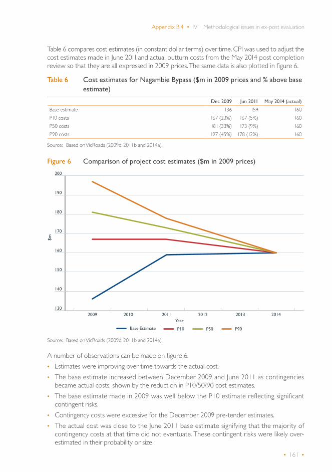
• 161 •


Table 6 compares cost estimates (in constant dollar terms) over time. CPI was used to adjust the cost estimates made in June 2011 and actual outturn costs from the May 2014 post completion review so that they are all expressed in 2009 prices. The same data is also plotted in figure 6.

Table 6 Cost estimates for Nagambie Bypass ($m in 2009 prices and % above base estimate)

Dec 2009 Jun 2011 May 2014 (actual)

Base estimate 136 159 160P10 costs 167 (23%) 167 (5%) 160P50 costs 181 (33%) 173 (9%) 160P90 costs 197 (45%) 178 (12%) 160

Source: Based on VicRoads (2009d; 2011b and 2014a).

Figure 6 Comparison of project cost estimates ($m in 2009 prices)

Source: Based on VicRoads (2009d; 2011b and 2014a).

A number of observations can be made on figure 6. • Estimates were improving over time towards the actual cost.• The base estimate increased between December 2009 and June 2011 as contingencies

became actual costs, shown by the reduction in P10/50/90 cost estimates.• The base estimate made in 2009 was well below the P10 estimate reflecting significant

contingent risks.• Contingency costs were excessive for the December 2009 pre-tender estimates. • The actual cost was close to the June 2011 base estimate signifying that the majority of

contingency costs at that time did not eventuate. These contingent risks were likely over-estimated in their probability or size.

130

140

150

160

170

180

190

200

P90P50P10Base Estimate

2009 2011Year

2012 20132010 2014

$m

• 162 •


Evans & Peck was commissioned by the Department in 2010 to review compliance of the Nagambie Bypass pre-tender cost estimate (December 2009) with the principles and procedures outlined in the Best Practice Cost Estimation for Publicly Funded Road and Rail Construction (Evans and Peck 2008) (the guidelines). Key findings on estimate preparation, contingency methodology and price escalation are highlighted below.

2 These values were incorrectly calculated. They should be slightly lower (33% and 45% respectively as reported in table 6).

Estimate preparation• For construction works, VicRoads used the practice of “all-up” historical rates that included all

contractor costs and margins (on-costs) related to the measured quantity of work. • While this methodology was not precluded from conforming to the guideline, it was not Evans

& Peck’s preferred method or the preference of industry or other agencies, particularly for medium to large projects and projects at a pre-tender estimate stage. The main reason for this was that cost estimates based on the “all-up” historical rates tend to lack transparency.

• The preferred method uses a first principle approach to estimating.

Contingency• The amount of contingency on top of the base estimate was estimated to be 34% at P50

and 46% at P90.2 These contingency estimates appeared excessive for a project at the pre-tender stage compared to other projects of a similar size and scope.

• Limited or no assessment has been made of contingent risks (such as political, environmental, latent conditions, contractual, adverse weather etc.)

Escalation• The escalation calculation is excessive as the cash flow extends well beyond the milestone

completion dates stated in the PPR. Completed work would not continue to attract price escalations as all construction costs have been incurred.

• The escalation rate in the November and December 2009 PPRs was specified in the linear form, which was not in line with the guidelines. These require escalation in a compound form.

In the process of undertaking this ex-post case study, VicRoads made a number of comments on the Evans & Peck (2010) review which are summarised below:• The consultants’ investigations and procedures were not accepted by VicRoads as there was

no evidence that their suggested approach was superior. • The high contingency in the initial cost estimate took into account the possibility that a large

amount of fill might need to be transported to the site if contractors weren’t able to gain access to a private quarry. The owner of the quarry had refused to enter into an agreement with the project office at the time when the initial project cost estimates were prepared.

• Evans & Peck’s cost estimating approach reflects a quantity surveyor approach rather than one from a civil engineering cost expert.

• The Nation Building Unit subsequently revamped and revised their advice to jurisdictions on how cost estimates should be carried out which was less aligned to the recommendations and findings contained in the Evans & Peck (2010) report.

• 163 •


Time and knowledge constraints in the ex-post evaluation team meant cost estimation issues for this project weren’t investigated further. The project review team in the Department of Infrastructure, Regional Development and Cities may be in a better position to review this (if required) as it has a strong focus on project cost review.

Residual valuesResidual values (RVs) capture the remaining benefits that the project may offer beyond the evaluation period. However the ex-ante analysis did not include residual value estimates and so under-estimated the project benefits.

In this ex-post evaluation, RVs were estimated using five methods: • straight-line depreciation (SLD)• component method• decreasing net benefits (DNB)• constant net benefits (CNB) • increasing net benefits (INB).

Appendix E of the main report describes each of these methodologies.

The SLD method was adopted as the reference for this study and estimates from other methods were used for sensitivity testing.

Estimation of RVs requires an assumption about the length of project life. Different components of the project have different lifespans with different costs. It was assumed that the average lifespan of the project was 50 years. This was based on previous estimates where a road project is expected to have an economic life of 40 to 60 years (Queensland Department of Transport and Main Roads, 2011, Transport for NSW 2013 and Austroads 2003).

FYRRThe required project evaluators for a road infrastructure project are the NPV and benefit-cost ratio (BCR). For non-mutually exclusive options, BCR is usually the deciding metric. However, investment timing is also an important factor to consider. The first-year rate of return (FYRR) test is useful for this purpose. The original analysis did not calculate or report FYRR as a performance evaluator; this is calculated in table 7 using the P90 CBA results contained in the VicRoads PPR lodged in December 2009 (2009c).

Table 7 Ex-ante first-year rate of return @ 4%

%

First-year net benefits ($m) 4.15Discounted first-year net benefits ($m) 3.34Discounted construction costs ($m) 172.18FYRR (%) 1.98

• 164 •


Delay for optimal timing refers to the number of years needed to delay a project until the discounted first-year net benefits are greater than or equal to 4% of the discounted construction costs. Figure 7 shows the ex-ante FYRR never rises above the threshold rate of 4% during the evaluation period, disregarding the spike caused by rehabilitation costs in the base case.

Figure 7 Ex-ante first year rate of return @ 4%

Note: The spike in FYRR in the 19th year was due to the large base case rehabilitation cost being avoided under the project case.

ExternalitiesEx-ante CBAs included some minor external benefits associated with reductions in greenhouse gas and other emissions (nitrogen oxides, carbon monoxide, non-methane volatiles and sulphur oxides). No other forms of externalities were considered in the analyses. The same methodology was adopted in the ex-post evaluation to estimate externality effects.

Base and price yearThe price year was set to 2009 in this ex-post analysis, the same as the ex-ante CBA.

The base year in the ex-ante analysis was stated as 2008 in the PPR and the CBA results table incorrectly labelled the base year as 2010. The actual base year used in ex-ante CBA calculations was 2009. In the ex-post analysis, the base year was set to 2009, the same as the price year.

Discount rateThe discount rate used in the ex-ante CBA was 4.4%. For consistency, the reference rate used in the ex-post CBA for discounting was set to 4% with 7% for sensitivity testing.

-2%

0%

2%

4%

6%

8%

10%

12%

14%

Delay (years)0 5 25 3010 15 20

FYR

R

• 165 •

V Reconstruction of the ex-ante CBA

The ex-ante CBA was replicated without any difficulty from the VicRoads EVAL4 spreadsheet documentation.

• 167 •


For consistency with other case studies, the ex-ante analysis was replicated at a 4% discount rate before any updates were made. The following adjustments were made to the ex-ante CBA:E1. Correcting spreadsheet errorsE2. Adjusting road length and width E3. Increasing the length of evaluation periodE4. Updating project and maintenance costsE5. Revising traffic forecastsE6. Re-allocating bypass trafficE7. Updating accident rate E8. Including residual values

A sensitivity test was also conducted using a 7% discount rate.

E1 – Correcting spreadsheet errorsTwo spreadsheet errors were amended in E1:• removing the abnormal spike in the annual road user benefit stream shown in figure 3• correcting the base year used for discounting the project costs.

Table 8 reports the effects of these adjustments on CBA outcome. Removing the spike in the road user benefits that occurred in the fourth year of the analysis period resulted in a significant fall in project benefits. Discounted road user benefits fell by 15%. Most of this was caused by falling VOC and travel time cost savings.

The change in base year to 2009 did not affect benefits as they were already discounted correctly. The costs however were erroneously discounted in the ex-ante CBA using 2008 as the base year. Changing the base year to 2009 increased the project costs by 4% as expected.

Falling road user benefits and rising project costs led to a decrease in the NPV (–30%). The BCR fell from 0.49 to 0.37.

• 168 •


Table 8 Correcting spreadsheet errors (E1)

@4% discount rate ($m in 2009 prices) Ex-ante E1 E1/Ex-ante (%)


Capital costs 172.2 179.1 4.0Routine maintenance costs –0.9 –0.9 4.0Periodic maintenance costs 1.8 1.9 4.0Rehabilitation costs –10.0 –10.4 4.0Discounted benefits 80.7 62.6 –22.5

Car VOC savings 2.9 –1.3 –145.7Bus/truck VOC savings 10.3 5.5 –46.8Car TTS savings 48.3 42.9 –11.2Freight TTS savings 15.2 13.1 –14.3Accident savings 3.6 2.7 –26.3Greenhouse gas savings 0.2 –0.2 –178.1Other gas savings 0.1 0.0 –100.9Residual value 0.0 0.0 N/ANet Present value (NPV) –82.4 –107.1 30.0


First-year rate of return (FYRR %) 1.98 1.90

E2 – Road length and width adjustmentsThe E2 update reduced the road length from 18km to 17km (–5.9%) and the width of the base case road sections from 22m to 7m (–68.2%).

The shorter road length reduced the amount of road user benefits generated across all road user cost categories, leading to a 4% fall in the total discounted benefits. Reduction in the base case road width led to lower maintenance and rehabilitation costs required for the base case road. As a result of these adjustments, the total project costs increased by 7.6% (table 9).

Corrections to road specifications caused the NPV to decline by 14.4% and the BCR to fall slightly from 0.37 to 0.33.

Table 9 Adjusting road length and width (E2)

@4% discount rate ($m in 2009 prices) E1 E2 E2/E1 (%)


Capital costs 179.1 179.1 0.0Routine maintenance costs –0.9 2.4 –356.2Periodic maintenance costs 1.9 4.2 121.5Rehabilitation costs –10.4 –3.1 –69.9Discounted benefits 62.6 60.1 –4.0

Car VOC savings –1.3 –1.4 3.9Bus/Truck VOC savings 5.5 5.2 –4.8Car TTS savings 42.9 41.5 –3.3Freight TTS savings 13.1 12.6 –3.4Accident savings 2.7 2.4 –12.2

Continued…

• 169 •


@4% discount rate ($m in 2009 prices) E1 E2 E2/E1 (%)

Greenhouse gas savings –0.2 –0.2 1.5Other gas savings 0.0 0.0 0.0Residual value 0.0 0.0 N/ANet present value –107.1 –122.5 14.4

Benefit-cost ratio 0.37 0.33


E3 – Extending the length of evaluation periodExtension of the evaluation period from 30 years to 34 years had the expected effect of increasing the project benefits (4.2%, table 10). The total discounted VOC savings fell due to the negative VOC savings for both cars and heavy vehicles from 2034. The negative savings were a result of the worsening condition of the project case road compared to the newly rehabilitated base case road in the later years.

A minor increase in discounted costs was incurred as the longer evaluation period took into account an extra four years of routine maintenance cost for the project. Extending the length of the evaluation period improved the NPV by 1.8% resulting in a slightly higher BCR (from 0.33 to 0.34).

Table 10 Extension of evaluation period (E3)



Capital costs 179.1 179.1 0.0Routine maintenance costs 2.4 2.7 11.8Periodic maintenance costs 4.2 4.2 0.0Rehabilitation costs –3.1 –3.1 0.0Discounted benefits 60.1 62.6 4.2

Car VOC savings –1.4 –2.2 59.0Bus/truck VOC savings 5.2 4.5 –14.9Car TTS savings 41.5 44.9 8.1Freight TTS savings 12.6 13.2 4.7Accident savings 2.4 2.6 9.8Greenhouse gas savings –0.2 –0.2 26.6Other gas savings 0.0 0.0 0.0Residual value 0.0 0.0 N/ANet present value (NPV) –122.5 –120.2 –1.8



E4 – Updating project costs and maintenanceThe actual project cost was $170m (outturn) compared with a budgeted cost of $222m (P90, outturn). On a constant price basis and in discounted terms, this was equivalent to a cost reduction of 17.6% (table 11).

• 170 •


The condition for one of the bypass carriageways was incorrectly set to worsen during construction in the ex-ante CBA. Correcting this error resulted in a slight fall in maintenance costs (10 to 21%) and improved road user benefits (6.9%) due to better road condition in the project case.

The above revisions improved the project NPV by 30.7%, increasing the BCR from 0.34 to 0.45.

Table 11 Update of project costs (E4)



Capital costs 179.1 147.5 –17.6Routine maintenance costs 2.7 2.1 –21.2Periodic maintenance costs 4.2 3.8 –9.9Rehabilitation costs –3.1 –3.1 0.0Discounted benefits 62.6 67.0 6.9

Car VOC savings –2.2 –1.8 –20.1Bus/truck VOC savings 4.5 5.3 19.1Car TTS savings 44.9 45.7 2.0Freight TTS savings 13.2 13.5 2.2Accident savings 2.6 2.6 0.0Greenhouse gas savings –0.2 –0.2 –9.5Other gas savings 0.0 0.0 0.0Residual value 0.0 0.0 N/ANet present value (NPV) –120.2 –83.3 –30.7



E5 – Revising traffic forecastsThe traffic update involved:• lowering the base year (2009) traffic level from an AADT of 6,774 to 6,697 • increasing the traffic growth rate from 1.43% a year (linear, 2009 as the base year) to a higher

compound growth of 2.5% a year.

The results of these changes are summarised in table 12. Lowering the traffic volume for the base year and raising traffic growth forecasts had a net effect of improving travel time savings for both cars (35.1%) and buses/trucks (99.8%), and accident cost savings (23.1%).

Table 12 Revising traffic forecasts (E5)



Capital costs 147.5 147.5 0.0Routine maintenance costs 2.1 2.1 0.0Periodic maintenance costs 3.8 3.8 0.0Rehabilitation costs –3.1 –3.1 0.0Discounted benefits 67.0 97.8 46.0

Car VOC savings –1.8 –2.8 55.2Continued…

• 171 •



Bus/Truck VOC savings 5.3 8.7 64.2Car TTS savings 45.7 61.8 35.1Freight TTS savings 13.5 27.0 99.8Accident savings 2.6 3.2 23.1Greenhouse gas savings –0.2 –0.2 –22.2Other gas savings 0.0 0.0 0.0Residual value 0.0 0.0 N/ANet Present value (NPV) –83.3 –52.5 –37.0



VOC savings for buses and trucks increased significantly (64.2%), while the negative savings in VOC for cars fell further (55.2%). Figure 8 shows the relationship between unit VOC and operating speed for different vehicle types at NRM = 40 in EVAL4. The operating speed for minimum VOC is 50km an hour for cars, 70km an hour for light trucks (2–axle rigid) and 90km an hour for heavy trucks (6–axle articulated).

Assume that in the base case vehicles travelled at the speed limit of 60km an hour within the town centre. Increased initial traffic levels and higher traffic growth forecasts would cause congestion in the base case road reducing the speed below 60km an hour. According to figure 8, a lower speed would reduce the unit VOC for cars for the base case, thereby increasing the VOC dis-savings for the project. There would be an opposite effect for trucks. A reduced speed would increase unit VOC in the base case, thereby increasing VOC savings for trucks.

Overall adjustments to the initial traffic level and the traffic growth rate led to a significant increase in road user benefits, lifting the BCR from 0.45 to 0.65.

Figure 8 VOC as a function of operating speed for a road condition NRM = 40

80

85

90

95

100

105

110

115

Heavy Truck Light Truck

LT/H

T V

OC

(cen

ts/k

m)

40 1009080706050

19

20

21

22

23

24

Car

Car

VO

C (c

ents

/km

)

Operating Speed (km/hr)

40 1009080706050

• 172 •


E6 – Re-allocating bypass trafficIn E6, 80% of through traffic was allocated to the bypass route instead of 100% as in the ex-ante analysis. Reduced bypass traffic led to a reduction of project benefits by 10%. The NPV dropped by 18.7% with the BCR falling from 0.65 to 0.59.

Table 13 Traffic split (E6)


Discounted costs 150.3 150.3 0.0Capital costs 147.5 147.5 0.0Routine maintenance costs 2.1 2.1 0.0Periodic maintenance costs 3.8 3.8 0.0Rehabilitation costs –3.1 –3.1 0.0Discounted benefits 97.8 87.9 –10.0

Car VOC savings –2.8 –1.1 –60.5Bus/Truck VOC savings 8.7 8.3 –5.0Car TTS savings 61.8 54.0 –12.6Freight TTS savings 27.0 23.7 –12.2Accident savings 3.2 2.9 –10.3Greenhouse gas savings –0.2 0.1 –173.6Other gas savings 0.0 0.1 171.3Residual value 0.0 0.0 N/ANet Present value (NPV) –52.5 –62.3 –18.7



E7 – Updating accident rateThe base case accident rate was changed from 0.12 to 0.08 crashes per MVKT. The project case accident rate was kept unchanged at 0.08 crashes per MVKT. As a result of this adjustment, the safety benefit estimate became negative (table 14). Higher average unit crash costs associated with the higher travel speeds in the project case were responsible for this outcome. Reduced safety benefits caused the NPV to fall by 16.1%. The BCR declined from 0.59 to 0.52.

Table 14 Updating base case accident rate (E7)



Capital costs 147.5 147.5 0.0Routine maintenance costs 2.1 2.1 0.0Periodic maintenance costs 3.8 3.8 0.0Rehabilitation costs –3.1 –3.1 0.0Discounted benefits 87.9 77.9 –11.4

Car VOC savings –1.1 –1.1 0.0Bus/truck VOC savings 8.3 8.3 0.0Car TTS savings 54.0 54.0 0.0Freight TTS savings 23.7 23.7 0.0

Continued…

• 173 •



Accident savings 2.9 –7.2 –352.9Greenhouse gas savings 0.1 0.1 0.0Other gas savings 0.1 0.1 0.0Residual value 0.0 0.0 0.0Net present value (NPV) –62.3 –72.4 –16.1

Benefit-cost ratio (BCR) 0.59 0.52First-year rate of return (FYRR %) 2.10% 1.82%

E8 – Residual ValuesThe ex-ante analysis did not include any RV estimates. For this ex-post evaluation, the SLD approach was used as a reference method. Other RV estimation methods were used for the purpose of sensitivity testing.

Table 15 shows the impact of including RV on the CBA outcome. As seen, including the SLD–based RV estimate added $19.8m to the project benefits. This estimate was likely to be over-stated due to the updated BCR being below 1. The sensitivity test showed the component method produced a similar result however estimates based on the net benefit approaches varied considerably from $16.8m–$39.6m representing 18–34% of total discounted benefits.

Inclusion of the SLD–based RV improved the NPV of the project by 27.3% and raised the BCR to 0.65.

Table 15 Inclusion of residual values (E8)


E7 Residual values

RV–EA RV1(SLD) RV2(C) RV2(DNB) RV3(CNB) RV4(INB)

Discounted costs 150.3 150.3 150.3 150.3 150.3 150.3

Capital costs 147.5 147.5 147.5 147.5 147.5 147.5Routine maintenance costs 2.1 2.1 2.1 2.1 2.1 2.1Periodic maintenance costs 3.8 3.8 3.8 3.8 3.8 3.8Rehabilitation costs –3.1 –3.1 –3.1 –3.1 –3.1 –3.1Discounted benefits 77.9 97.6 97.6 94.7 109.1 117.4

Car VOC savings –1.1 –1.1 –1.1 –1.1 –1.1 –1.1Bus/Truck VOC savings 8.3 8.3 8.3 8.3 8.3 8.3Car TTS savings 54.0 54.0 54.0 54.0 54.0 54.0Freight TTS savings 23.7 23.7 23.7 23.7 23.7 23.7Accident savings –7.2 –7.2 –7.2 –7.2 –7.2 –7.2Greenhouse gas savings 0.1 0.1 0.1 0.1 0.1 0.1Other gas savings 0.1 0.1 0.1 0.1 0.1 0.1Residual value 0.0 19.8 19.8 16.8 31.2 39.6

(RV as % of total benefits) 0% 20% 20% 18% 29% 34%

Net present value (NPV) –72.4 –52.6 –52.6 –55.6 –41.2 –32.8

Benefit-cost ratio (BCR) 0.52 0.65 0.65 0.63 0.73 0.78

• 174 •


E9 – Discount rateChanging the discount rate to 7% reduced construction costs as well as recurring maintenance and rehabilitation costs. As expected, discounted benefits were also reduced considerably, falling by 42.7%. The higher discount rate reduced BCR from 0.65 to 0.40.

Table 16 Discount rate sensitivity test at 7% (E9)



Capital costs 147.5 139.1 –5.7Routine maintenance costs 2.1 1.2 –43.4Periodic maintenance costs 3.8 2.0 –48.0Rehabilitation costs –3.1 –1.6 –49.5Discounted benefits 97.6 55.9 –42.7

Car VOC savings –1.1 –0.3 –73.8Bus/truck VOC savings 8.3 5.9 –29.1Car TTS savings 54.0 32.0 –40.8Freight TTS savings 23.7 14.2 –40.2Accident savings –7.2 –4.4 –39.0Greenhouse gas savings 0.1 0.1 –17.3Other gas savings 0.1 0.0 –32.8Residual value 19.8 8.4 –57.4Net present value (NPV) –52.6 –84.7 61.0

Benefit-cost ratio (BCR) 0.65 0.40First-year rate of return (FYRR%) 1.82% 1.67%

SummaryFigure 9 shows the total variation in NPV for the Nagambie Bypass project between the ex-ante and ex-post evaluations, and its sources. The NPV was estimated to be –$82.4m in the ex-ante CBA (at 4% discount rate) and has been revised upwards to –$52.6m in this ex-post evaluation.

• 175 •



Major contributors to the NPV under-estimation for the project were over-estimation of project (and maintenance) costs (E4), under-estimation of traffic growth (E5) and failure to include a RV (E7). These factors added a total of $87.5m to the project NPV. Extending the evaluation period (E3) also improved the NPV, though marginally. Correcting spreadsheet errors (E1) and adjusting road specifications (E2) and traffic allocation (E6) together reduced the project NPV by $49.9m. The update of the base case accident rate (E6) further reduced the estimated NPV by $10.1m.

The net effect of these variations is the addition of $29.8m to the project NPV. Despite these revisions the ex-post NPV remained negative confirming the Nagambie bypass was not an economically viable project.

-30

-20

-10

0

10

20

30

40

$m

E7-E8(Including

residual values)

E6-E7(Updating

accident rate)

E5-E6(Re-allocating bypass traffic)

E4-E5(Revising

traffic forecasts)

E3-E4(Updating project andmaintenance

costs)

E2-E3(Increasing the length

of ealuationperiod)

E1-E2(Adjustingroad lengthand width)

EA-E1(Correcting spreadsheet

errors)

-15.4

2.3

35.132.6

19.8

-10.1-9.8

-24.7

Total Variation = $149.8mEx-ante NPV = -$82.4mEx-post NPV = -$52.6m

• 177 •

VII Lessons learnt

This section draws out the lessons for future economic evaluation from the review of the ex-ante CBA and the ex-post evaluation.

CBA reportingThe case study showed that there was much room for improvement in the quality of CBA reporting. Quoted figures in PPRs were inconsistent with those contained in the attached CBA summary tables. There was no separate CBA report for the project, making review difficult. PPRs for large projects should be accompanied with a separate CBA report that details inputs and methodology with a discussion of results for transparency. Having such a report would have helped identify errors in EVAL4 applications.

Review of ex-ante CBAsThere were some simple spreadsheet errors that had significant impacts, and these could have been detected by plotting annual benefit and cost streams in a review process. Most others were data input error, which could have been discovered by cross-checking.

Inconsistencies in CBA results were seen across the PPRs from August 2009, November 2009, December 2009 and June 2011. These variations were not explained in the PPRs even when differences were extreme: for example, a four-fold reduction in safety benefits from the November to December 2009 PPR (table 1). New PPRs or CBAs should include an update to explain significant changes from the earlier results.

Traffic allocationFor any bypass project, allocation of traffic between the existing road and the new road is critically important to achieve sensible CBA results. While the assumption of a 100% allocation of traffic to the bypass is convenient from a modeling perspective, it is unrealistic and should not have been accepted. In future, more effort should be made to justify the assumed split in traffic between the base case road and bypass road.

Road condition and maintenanceThis case study demonstrates the significant effect road condition can have on road user costs, particularly VOCs. The sharp fall and subsequent decline of net benefits for the project in later years was due to the effect of road condition on road user costs modelled in EVAL4. This result has not been born out in other case studies. Consensus on the effects of road condition on road user costs is required to ensure CBAs across road projects are comparable.

• 178 •


Residual valuesThe ex-ante CBA did not feature any RV for the project. RVs should be included in CBAs where asset lives extend well beyond the analysis period.

Both the asset depreciation and the net benefit approaches were used to estimate the RV in the ex-post evaluation. As expected, the net benefit approaches produced—in general—higher RV estimates that accounted for up to 34% of the total road user benefits. The exception to this was the decreasing net benefits method that produced an RV estimate smaller to those derived from the depreciation methods. This result demonstrates the tendency of the asset depreciation approach to over-estimate RVs for projects with BCRs below one.

FYRRProjects with traffic not subject to substantial congestion for initial years are unlikely to provide high enough benefits to pass the FYRR test. In cases where maintenance plays a large role in road user costs, multiple optimal timings may be present due to changes in road condition from major maintenance. In such situations, separate CBAs must be performed for these timings. NPVs can be compared to determine the optimal project timing (see ATC 2006 for more detailed discussion).

• 179 •


BITRE 2009, National Road Network Intercity Traffic Projections to 2030 – Working Paper 75, February.

Evans & Peck 2008, Best Practice Cost Estimation for Publicly Funded Road and Rail Construction, June.

Evans & Peck 2010, Nation Building: Review of Compliance of Nagambie Bypass Pre-tender Cost Estimate with Guidelines Compliance Report, February.

Veitch Lister Consulting, Traffic Modelling and Analysis Report – Goulburn Valley Highway Nagambie Bypass, December

VicRoads 2009a, Nagambie Bypass Project Proposal Report Construction Stage, August.

VicRoads 2009b, Nagambie Bypass Project Proposal Report Construction Stage, November.

VicRoads 2009c, Nagambie Bypass Project Proposal Report Construction Stage, December.

VicRoads 2009d, Nagambie Bypass Project Cost Estimate Input, June.

VicRoads 2011a, Nagambie Bypass Project Proposal Report Construction Stage, June.

VicRoads 2011b, Nagambie Bypass Project Cost Estimate Input, June.

VicRoads 2014a, Post Completion Report, May.

VicRoads 2014b, Traffic Volume Data for Victoria, July.

VicRoads 2015, Nagambie Bypass – Post Completion Evaluation Report, June.



Northern Expressway

Appendix B.5


• 183 •

Contents

Summary ...................................................................................................................................................................189

I Introduction ..............................................................................................................................................................191

II Description of the Northern Expressway project ..........................................................................193


Ex-ante CBAs ...................................................................................................................................195

Review of DTEI 2007 CBA study .........................................................................................196

IV Accuracy of ex-ante traffic forecasts and CBA .................................................................................201

Parsons Brinckerhoff (2011) study ........................................................................................201

Accuracy of ex-ante traffic forecasts ..................................................................................207

Accuracy of ex-ante travel time saving predictions ....................................................211

V Lessons learnt .........................................................................................................................................................217

CBA reporting .................................................................................................................................217

Traffic analysis ...................................................................................................................................217

Travel time modelling ...................................................................................................................218


• 185 •

List of tables

Table 1 Ex-ante CBAs for the proposed Northern Expressway project ......................... 195

Table 2 Traffic forecasts for the base case and project case .................................................... 197

Table 3 Travel time savings for the Northern Expressway project (minutes) ...............206

Table 4 Ex-ante traffic forecasts for the base case (vehicles per day, 2006–2011) .....207

Table 5 Growth of annual average daily traffic on the Northern Expressway (per cent per year) .........................................................................................................................208

Table 6 Travel time savings for the Northern Expressway project (2010–11) .............. 211

Table 7 Assumptions about future traffic growth and congestion ....................................... 214

• 187 •

List of figures

Figure 1 Proposed Northern Expressway project ..........................................................................194

Figure 2 Annual travel time cost savings (in 2006 prices) ...........................................................198

Figure 3 Growth in annual travel time savings (% change over the previous year)...... 198

Figure 4 Annual VOC savings (in 2006 prices) ..................................................................................199

Figure 5 Travel time survey routes ...........................................................................................................203

Figure 6 Traffic impacts of Northern Expressway ...........................................................................205

Figure 7 Forecast traffic volumes over actual observations (%, 2011) .................................208

Figure 8 Actual and forecast traffic volumes on the Northern Expressway ....................209

Figure 9 Travel time cost savings: ex-post versus ex-ante ($m) .............................................. 215

• 189 •

Summary

The ex-post evaluation of the Northern Expressway project forms part of the second round of case studies undertaken by the Bureau of Infrastructure, Transport and Regional Economics (BITRE) of road investment projects on the National Land Transport Network. This case study was undertaken in consultation with SA Department of Planning, Transport and Infrastructure (DPTI). Objectives were to assess the economic performance of the Northern Expressway project and to check the accuracy of the ex-ante cost-benefit analysis (CBA).

The project was to construct the new 23 kilometre-long Northern Expressway and upgrade 15 kilometres of the existing Port Wakefield Road. The project was completed in 2010 within the budget of $564 million (outturn).

Unlike other studies which involved full ex-post evaluation, this case study focused largely on reviewing the ex-ante CBA and checking the accuracy of ex-ante travel time saving estimates using readily available information. A number of lessons can be learnt:

CBA reporting: a series of CBAs were performed for the project, but the differences were not discussed in the final CBA for decision making. The significant fluctuation in travel time saving estimates contained in the scoping and development Project Proposal Report (PPR) should have been clearly explained. Doing this would have helped reduce errors and improved decision making.

CBA documentation for the project comprised the PPR and printout of CBA spreadsheets as one of the PPR’s appendices. For a project worth over half a billion dollars, a more detailed self-contained CBA report should have been requested to facilitate review and decision making.

The ex-ante CBA report should have provided a critical review of traffic modelling results before they were used as inputs for the CBA. This is especially true for those inputs directly impacting travel time cost savings. Such a review could include: • a summary of modelled (or assumed) traffic growth forecasts for both the base and project

cases (see tables 4 and 5 as an example)• a graph of modelled growth in travel time savings over time (see figure 3)• a summary of travel speed/time impacts for key affected roads as it is difficult to gauge

plausibility of travel time saving estimates reported at the highly aggregated level.

With this review, questions could then be asked about the reasonableness of the traffic modelling results.

Traffic analysis: there was significant over-estimation of traffic demand for the opening year and, to a lesser extent, for the years beyond, which in turn could lead to over-estimation of

• 190 •


congestion impacts. The reasons for this could not be identified without undertaking a detailed ex-post traffic modelling within the MASTEM. Valuable lessons could have been learnt if such modelling had been undertaken.

Travel time modelling: Travel time savings were over-estimated due to overly optimistic traffic forecasts. It was not clear whether the modelling methodology itself was also a contributor factor.

The simplified methodology developed in this case study, while rough, can be useful to crosscheck results derived from complex traffic models. It can also provide faster analyses with minimum data requirements. However, this should only be used as a last resort in the absence of any other alternatives.

• 191 •

I Introduction

The Northern Expressway case study forms part of BITRE’s second round of ex-post cost-benefit analysis (CBA) of road investment projects on the National Land Transport Network. The case study was implemented by BITRE in consultation with the SA Department of Planning, Transport and Infrastructure (DPTI, formerly known as DTEI).

The objectives are to:• assess the economic performance of the project• check the accuracy of ex-ante CBA • explain differences (if any) in results between the ex-ante and ex-post CBAs • draw lessons from the case study to improve future CBAs.

As part of the ex-post economic evaluation, this case study provided an opportunity to review the performance of an urban transport model to predict the base case travel demand and assess the impact of a major piece of infrastructure investment in an urban environment. Data on travel times on key existing roads and the newly-built expressway were used to scrutinise travel time saving estimates from the Metropolitan Adelaide Strategic Transport Evaluation Model (MASTEM), an urban transport planning model for Adelaide.

The following section provides an overview of the Northern Expressway project. Section 3 reviews the ex-ante CBA analyses undertaken by Department for Transport, Energy and Infrastructure (DTEI, now known as DPTI). Section 4 checks the accuracy of ex-ante traffic forecasts and travel time saving estimates using actual observed information and more recent traffic forecasts. Lessons learnt are discussed in the final section.

• 193 •

II Description of the Northern Expressway project

The Northern Expressway project consists of two components: the Northern Expressway and the Port Wakefield Road Upgrade. The Northern Expressway is a new 23 kilometre four-lane road with a pedestrian and cycle path linking the Gawler Bypass with Port Wakefield Road. It has a number of bridges and overpasses that cross over existing roads.

The Port Wakefield Road Upgrade involves improvements at key intersections between Waterloo Corner Road and Salisbury Highway. The main objective of this project is to provide a fast freight corridor between Sturt Highway and Port Adelaide while relieving pressure on the existing road network, particularly along Main North Road and Angle Vale/Heaslip roads.

The project was completed in September 2010 within the budget of $564m. The Northern Expressway is now known as the Max Fatchen Expressway (M20).

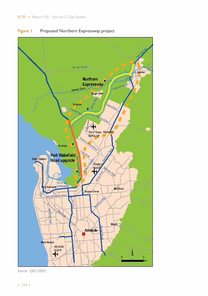
• 194 •


Figure 1 Proposed Northern Expressway project

Source: QED (2007)

• 195 •


A brief history of the economic evaluation undertaken for the Northern Expressway project is provided in this section with a detailed review of the Department for Transport, Energy and Infrastructure (DTEI) August 2007 CBA study, which was the basis for the decision to proceed with the project.

Ex-ante CBAsBefore the Australian Government’s decision to fund construction of the Northern Expressway, there had been three CBAs on the economic viability of the project (table 1).

Table 1 Ex-ante CBAs for the proposed Northern Expressway project

($m @ 7%) October 2005 December 2006 August 2007

Project phase Scoping Development DeliveryDiscounted benefits 462.7 886 895

Travel time savings 456.5 965 927VOC savings –44.7 –167 –115Crash cost reductions 47.7 68 74Residual value 3.2 6 2Externality benefits 0 14 7Discounted costs 214.2 553 360

Capital expenditure 209.7 566 377Maintenance 4.5 –13 –17Net present value 248.5 333 535

Benefit-cost ratio (BCR) 2.16 1.60 2.49

First-year rate of return (FYRR) 4.18

Source: DTEI (2005, 2007a and 2007b).

The first ex-ante CBA was conducted by DTEI and its results were reported in the scoping stage Project Proposal Report (PPR) lodged in October 2005 (DTEI 2005). The economic analysis was based on the concept for the Northern Expressway proposed as part of the SKM (1998) study. The analysis assumed a total project cost of $300m (outturn), comprising $190m for the Northern Expressway from Gawler to Waterloo Corner and $110m to upgrade Port Wakefield Road from a four lane arterial to a six lane freeway road.

Travel time savings were the main form of benefits, accounting for nearly 99% of the total road user cost savings. Travel time saving estimates were derived from DTEI’s urban traffic model. Negative vehicle operating cost (VOC) savings were associated with the longer distance that had to be travelled for the project case. Based on a discount rate of 7%, the net present value (NPV) of the project was estimated to be $248.5m and the benefit-cost ratio (BCR) 2.2.

• 196 •


The second ex-ante CBA was conducted in December 2006 and its results were quoted in the development stage PPR lodged in February 2007 (DTEI 2007a). The cost estimate was increased to $550m (outturn) in the December 2006 CBA due to a significant under-estimation of the project cost. This CBA also included a downscaling of the upgrade of Port Wakefield road with widening now limited to existing junctions, intersections and limited access mid-block sections. The CBA included a second stage of development for the construction of the Port Wakefield Expressway (now called the Northern Connector, currently under construction), a new route running west of Port Wakefield Road linking the Northern Expressway and the Port River Expressway. The P90 cost of the project for both stages was estimated to be $850m in outturn dollar terms with the Port Wakefield Expressway cost ($300m) being preliminary. The discounted project cost (@7%) was calculated to be $566m made up of $356m for stage 1 (Northern Expressway and limited widening of Port Wakefield Road) and $210m for stage 2 (Port Wakefield Expressway). The construction of the Port Wakefield Expressway was expected to result in additional benefits for the Northern Expressway project by attracting more traffic.

Compared with the first ex-ante CBA (DTEI 2005), the total road user benefits estimated in the second ex-ante CBA (DTEI 2007a) increased by 91%. This was largely caused by a surge in estimated travel time savings, rising from $456.5m (in 2004 prices) to $965m (in 2006 prices) (table1). Because of a larger increase in the project costs, the estimated BCR in the second ex-ante CBA was lower (1.6).

The third ex-ante CBA was conducted in August 2007 and its results were quoted in the PPR for project delivery lodged in September 2007 (DTEI 2007b). The total P90 cost estimate was $564m in outturn dollar terms, $472m in 2006 prices and $360m discounted, which was one third less than that specified in the second ex-ante CBA. The reason for this was the exclusion of project costs associated with the construction of the Port Wakefield Expressway. Travel time cost saving estimates were slightly lower than those estimated in the second ex-ante CBA (DTEI 2007a). As a result, there was a noticeable improvement in the estimated BCR, from 1.6 to 2.5. The first-year rate of return was calculated to be 4.2%.

Since the third ex-ante CBA (DTEI 2007b) was the basis on which the final decision was made to proceed with the project, it was the focus in our ex-post review.

Review of DTEI 2007 CBA studyAccording to the PPR (DTEI 2007b), preparation of the 2007 CBA followed the National Guidelines for Transport System Management (ATC 2006) and Austroads guide to project evaluation. The economic evaluation considered a project proposal comprising the Northern Expressway (to be constructed by December 2010) and the Port Wakefield Road (to be upgraded by December 2008). Unlike the second ex-ante CBA (DTEI 2007a), the evaluation did not include the construction of the new Port Wakefield Expressway by 2016.

Project benefits included:• travel time savings• VOC savings• crash cost reductions • externality benefits (ambient pollution, greenhouse gas emissions, noise, water pollution, nature

and landscapes, and urban separation).

• 197 •


No estimate was made of the benefits associated with the construction of the 23km cycle path along the Northern Expressway. The cycle path currently ends at Port Wakefield road, a high traffic area that is not ideal for cyclists and is likely to deter them from using this route.

Travel time cost savings were the dominant form of road user benefits for this project. Travel time and distance travelled with and without the project were estimated using a DTEI’s in-house traffic model. MASTEM produced aggregate outputs used to calculate road user benefits in years 2011, 2016 and 2021. Table 2 presents a summary of MASTEM outputs used in the DTEI 2007 CBA. As seen with the Northern Expressway, the network travel time was reduced though the distance travelled increased. Travel time savings per working day nearly doubled between 2011 and 2016 and more than tripled between 2011 and 2021. Dis-savings in distance travelled increased up to year 2016 and decreased thereafter. It was not clear what had caused this reversal.

No estimates of travel time or speed were provided for the key affected roads, making it difficult to gauge the plausibility of the overall impacts reported in table 2.

Table 2 Traffic forecasts for the base case and project case

Year

Travel time (hours/working day) Total travel time (hours/working day)

Travel distance (km/working day)Mid-block Intersections

Base case

2006 378 887 121 061 499 948 21 829 0802011 420 477 142 306 562 783 24 275 4002016 449 298 158 828 608 126 25 952 7602021 487 437 191 966 679 403 28 218 330

Project case

2011 420 404 137 253 557 657 24 358 7862016 449 079 149 122 598 201 26 159 2062021 487 118 175 024 662 142 28 376 521

Base case – project case

2011 73 5 053 5 126 –83 3862016 219 9 706 9 925 –206 4462021 319 16 942 17,261 –158 191

Source: DTEI (2007b).

To estimate the annual road user costs for the base and project cases, linear interpolation was used for years between 2011 and 2021, and linear extrapolation for years after 2021. Extrapolation of road user costs was based on the following assumptions:• for 2021–2031, at half the ‘2011–2021’ rate of increase • for 2031–2041, at a quarter the ‘2011–2021’ rate of increase.

Figure 2 shows annual travel time cost saving estimates for the final ex-ante CBA together with those from the first two ex-ante CBAs. As seen, the travel time cost savings for the 2007 CBA were generally lower than those estimated in the 2006 CBA (which included the effects of the new Port Wakefield Road from 2016), but significantly higher than those estimated in the 2005 CBA.

It appeared that growth in the estimated travel time cost savings for the final ex-ante CBA was excessive for the first 10 years of the evaluation period, ranging from nine to 19% a year (figure 3). No explanation was provided in the PPR for such high growth rates.

• 198 •


Figure 2 Annual travel time cost savings (in 2006 prices)

Note: Travel time cost saving estimates in 2005 CBA were adjusted to 2006 prices for the purpose of comparison.Source: DTEI (2005, 2007a and 2007b).

Figure 3 Growth in annual travel time savings (% change over the previous year)

Source: Derived by BITRE on the basis of DTEI (2007b).

0

50

100

150

200

250

CBA (Aug 2007)CBA (Dec 2006)Year

CBA (2005)

2005 202520202010 2015 20352030 2040

$m

0

2

4

6

8

10

12

14

16

18

20

% change over the previous year

2010 2030 20352015 2020 2025Year

2040

%

• 199 •


Trends in annual dis-savings in VOCs differed across the three ex-ante CBAs (figure 4). The reversal in VOC dis-savings in the 2007 CBA reflects the decreasing difference in the estimated distance travelled since 2016 between the base and project cases (table 2). The reason for such a reversal was not provided.

Figure 4 Annual VOC savings (in 2006 prices)

Note: Negative figures mean dis-savings in VOCs. Source: Derived by BITRE on the basis of DTEI (2007b).

A summary of the DTEI 2007 CBA output was provided as an appendix in the PPR lodged in September 2007. Given the size of the project, a detailed self-contained CBA report would have been useful for review and decision-making. There was also room for improvement in reporting and validating CBA inputs, as outlined above.

-30

-25

-20

-15

-10

-5

0

CBA (Aug 2007)CBA (Dec 2006)CBA (2005)

2005 202520202010 2015 20352030 2040Year

$m

• 201 •

IV Accuracy of ex-ante traffic forecasts and CBA

As travel time cost savings are the largest part of the road user benefits for the Northern Expressway project, the focus of this ex-post review is on checking the accuracy of travel time savings predicted by the MASTEM model.

Travel time savings are closely linked with the forecast traffic levels for both the base and project cases. A review of traffic forecasts produced by MASTEM for the key affected roads helps assess the plausibility of the ex-ante travel time saving estimates.

In 2011, Parsons Brinckerhoff conducted a Before and After Opening Study (Parsons Brinckerhoff 2011) on the Northern Expressway project for DTEI. This investigated the changes in traffic patterns in the Northern Adelaide Region including travel time savings attributable to the Northern Expressway. The results can be used to cross-check the accuracy of the ex-ante traffic forecasts and travel time saving estimates.

This section provides a summary of the key results of the Parsons Brinckerhoff (2011) study, which are then used to assess the accuracy of ex-ante traffic forecasts and travel time saving estimates.

Parsons Brinckerhoff (2011) studyThe work undertaken by Parsons Brinckerhoff (2011) comprised quantification of the following three components:• shifts in traffic volumes across the northern road network in response to the opening of

Northern Expressway• changes in traffic movements at key intersections within Northern Adelaide caused by route

shifts due to the opening of Northern Expressway• travel time savings attributable to the Northern Expressway project.

For the first two components, Parsons Brinckerhoff (2011) used the traffic data collected by DTEI just before and immediately after the opening of the Northern Expressway (13 September 2010). This included week-long classified midblock counts and intersection turning movement counts. Where counts were missing before the opening of the Northern Expressway, historical count data was adopted and adjusted to a common base. Counts undertaken before and after opening were conducted at the same location.

• 202 •


For the third component, Parsons Brinckerhoff conducted travel time surveys before and after the opening of the Northern Expressway using BluTripsTM1 technology (Parsons Brinckerhoff 2010). Surveys before the bypass opening were conducted between 2 and 10 September 2010 and those after opening between 21 and 29 October 2010. Travel times reported in Parsons Brinckerhoff (2011) were weekday averages for the duration of the surveys.

Travel times were recorded between the Sturt Highway at Gawler and three major destinations in Adelaide: Gepps Cross, Port Adelaide and Regency Park. Altogether travel times for 10 routes were recorded as shown in figure 5.

Each of the 10 routes is described in detail below.

1 Parsons Brinckerhoff ’s BluTripsTM travel time measurement system records media access control (MAC) addresses from Bluetooth capable vehicles at multiple locations and attaches a timestamp for each record. MAC addresses between receivers are matched and using the associated timestamps and receiver location, the travel time and speed can be determined.

• Gawler to Gepps Cross via the following routes (and in reverse direction):Route 1 – Main North Road.Route 2 – Main North Road, Salisbury Highway and Port Wakefield Road.Route 3 – Angle Vale Road, Heaslip Road, Waterloo Corner Road and Port Wakefield Road.Route 4 – Northern Expressway and Port Wakefield Road.

• Gawler to Port Adelaide (intersection of Port River Expressway and Perkins Drive) via the following routes (and in reverse direction):

Route 5 – Main North Road and Salisbury Highway.Route 6 – Angle Vale Road, Heaslip Road, Waterloo Corner Road, Port Wakefield Road and Salisbury Highway.Route 7 – Northern Expressway, Port Wakefield Road and Salisbury Highway.

• Gawler to Regency Park (intersection of South Road and Regency Road) via the following routes (and in reverse direction):

Route 8 – Main North Road, Salisbury Highway and South Road.Route 9 – Angle Vale Road, Heaslip Road, Waterloo Corner Road, Port Wakefield Road, Salisbury Highway and South Road.Route 10 – Nor thern Expressway, Por t Wakefield Road, Salisbury Highway and South Road.

Parsons Brinckerhoff (2011) reported traffic impacts of Northern Expressway in three main forms:• route shifts for total and heavy vehicle traffic• changes in movements at the key intersections • travel time impacts.

Findings from Parsons Brinckerhoff (2011) on route shifts for total traffic and travel time impacts are reproduced below.

• 203 •

Appendix B.5 • IV Accuracy of ex-ante traffic forecasts and CBA

Figure 5 Travel time survey routes

Source: Reproduced from Figure 3.7 in Parsons Brinckerhoff (2011).

• 204 •


Route shiftingThe route shifting in Northern Adelaide as a result of the opening of Northern Expressway is summarised in figure 6. It is measured by changes in total traffic flows across 10 screen lines. The main shifts in traffic volumes include:• a decline in total traffic volumes along Main North Road (related to route 1) ranging from

20% south of Gawler to 3% near Gepps Cross• a drop in total traffic volumes along Angle Vale Road and Heaslip Road (related to routes 3,

6 and 9) by 30–55%• a decrease in total traffic volumes along Salisbury Highway east of Port Wakefield Road

(related to routes 2, 5 and 8) by 2–5%• an increase in total traffic volumes along Port Wakefield Road by up to 80% (where Northern

Expressway joins Port Wakefield Road).

Travel time savingsTravel time savings attributable to the Northern Expressway project are summarised in table 3. Savings are reported for the AM and PM peak hours, and for business hours in both directions. The ‘before’ travel times for routes 4, 7 and 10 were simple averages of the ‘before’ travel times for alternative routes within the same origin-destination pairs. A number of conclusions emerge from table 3.• travel times for the full length on route 1 (via Main North Road) were reduced by 0.5–2.7

minutes per trip. This was a response to a reduction in traffic volumes on that road by 3–20% after the opening of Northern Expressway

• travel time savings were larger for routes 3, 6 and 9 (via Angle Vale Road and Heaslip Road) ranging from 4.7 to 5.2 minutes a full trip. This reflected larger reductions in traffic volumes (30–55%) on these routes following the opening of Northern Expressway

• travel time savings were insignificant for routes 2, 5 and 8 (via Salisbury Highway and Wakefield Road) reflecting a much smaller reduction in traffic volumes on these (2–5%) following the opening of Northern Expressway

• travel time savings for the full length on routes 4, 7 and 10 (vehicles using the Northern Expressway) were the largest (eight to nine minutes a trip).

Temporary speed restrictions were in place at several locations alongside Northern Expressway at the time when the travel time surveys were conducted. With these restrictions removed, Parsons Brinckerhoff (2011) expected additional travel time savings of 1 to 1.5 minutes for vehicles using Northern Expressway.

• 205 •


Figure 6 Traffic impacts of Northern Expressway

Source: Reproduced from Figure 3.1 in Parsons Brinckerhoff (2011) with traffic counts of interest numbered.

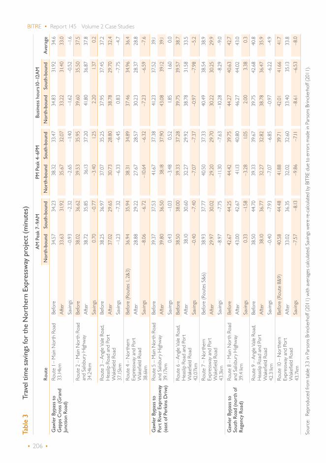
• 206 •

BITRE • Report 145 Volume 2 Case StudiesTa

ble

3 Tr

avel

tim

e sa

ving

s fo

r th

e N

orth

ern

Expr

essw

ay p

roje

ct (m

inut

es)

Rou

te

AM

Pea

k 7–

9AM

PM P

eak

4–6P

MBu

sine

ss h

ours

10–1

2AM

Ave

rage

Nor

th-b

ound

Sout

h-bo

und

Nor

th-b

ound

Sout

h-bo

und

Nor

th-b

ound

Sout

h-bo

und

Gaw

ler

Bypa

ss t

o

Gep

ps C

ross

(Gra

nd

Junc

tion

Roa

d)

Rout

e 1 –

Main

Nor

th R

oad

33.14

kmBe

fore

34.57

34.23

38.32

33.47

34.83

31.92

34.6

Afte

r33

.6331

.9235

.6732

.0733

.2231

.4033

.0Sa

vings

–0.93

–2.32

–2.65

–1.40

–1.62

–0.52

–1.6

Rout

e 2

– M

ain N

orth

Roa

d an

d Sa

lisbu

ry H

ighw

ay

34.24

km

Befo

re38

.0236

.6239

.5335

.9539

.6035

.5037

.5Af

ter

38.72

35.85

36.13

37.20

41.80

36.87

37.8

Savin

gs0.7

0–0

.77–3

.401.2

52.2

01.3

70.2

Rout

e 3

– An

gle V

ale R

oad,

Hea

slip

Road

and

Port

W

akefi

eld R

oad

37.15

km

Befo

re38

.2536

.9737

.0735

.2537

.9537

.4537

.2Af

ter

37.02

29.65

30.73

28.80

38.78

29.70

32.4

Savin

gs–1

.23–7

.32–6

.33–6

.450.8

3–7

.75–4

.7

Rout

e 4

– N

orth

ern

Expr

essw

ay an

d Po

rt

Wak

efield

Roa

d 38

.6km

Befo

re (R

oute

s 1, 2

&3)

36.94

35.94

38.31

34.89

37.46

34.96

36.4

Afte

r28

.8829

.2227

.6728

.5730

.2328

.3728

.8Sa

vings

–8.06

–6.72

–10.6

4–6

.32–7

.23–6

.59–7

.6

Gaw

ler

Bypa

ss t

o

Port

Riv

er E

xpre

ssw

ay

(eas

t of

Per

kins

Dri

ve)

Rout

e 5

– M

ain N

orth

Roa

d an

d Sa

lisbu

ry H

ighw

ay

39.17

km

Befo

re39

.3737

.5341

.6737

.3841

.2337

.5239

.1Af

ter

39.80

36.50

38.18

37.90

43.08

39.12

39.1

Savin

gs0.4

3–1

.03–3

.480.5

21.8

51.6

00.0

Rout

e 6

– An

gle V

ale R

oad,

Hea

slip

Road

and

Port

W

akefi

eld R

oad

42.07

km

Befo

re38

.5038

.0039

.3337

.2839

.7539

.5738

.7Af

ter

38.10

30.60

32.27

29.92

38.78

31.58

33.5

Savin

gs–0

.40–7

.40–7

.07–7

.37–0

.97–7

.98–5

.2

Rout

e 7

– N

orth

ern

Expr

essw

ay an

d Po

rt

Wak

efield

Roa

d 43

.3km

Befo

re (R

oute

s 5&6

)38

.9337

.7740

.5037

.3340

.4938

.5438

.9Af

ter

29.97

30.02

29.20

29.70

30.22

30.25

29.9

Savin

gs–8

.97–7

.75–1

1.30

–7.63

–10.2

8–8

.29–9

.0

Gaw

ler

Bypa

ss t

o

Sout

h R

oad

(nor

th o

f R

egen

cy R

oad)

Rout

e 8

– M

ain N

orth

Roa

d an

d Sa

lisbu

ry H

ighw

ay

39.41

km

Befo

re42

.6744

.2544

.4239

.7544

.2740

.6342

.7Af

ter

43.00

42.67

41.13

40.80

46.27

44.02

43.0

Savin

gs0.3

3–1

.58–3

.281.0

52.0

03.3

80.3

Rout

e 9

– An

gle V

ale R

oad,

Hea

slip

Road

and

Port

W

akefi

eld R

oad

42.31

km

Befo

re38

.5044

.7039

.3339

.6739

.7542

.6840

.8Af

ter

38.10

36.77

32.27

32.82

38.78

36.47

35.9

Savin

gs–0

.40–7

.93–7

.07–6

.85–0

.97–6

.22–4

.9

Rout

e 10

– N

orth

ern

Expr

essw

ay an

d Po

rt

Wak

efield

Roa

d 43

.7km

Befo

re (R

oute

8&9

)40

.5844

.4841

.8839

.7142

.0141

.6641

.7Af

ter

33.02

36.35

32.02

32.60

33.40

35.13

33.8

Savin

gs–7

.57–8

.13–9

.86–7

.11–8

.61–6

.53–8

.0

Sour

ce:

Repr

oduc

ed fr

om ta

ble 3

.3 in

Pars

ons B

rinck

erho

ff (2

011)

with

aver

ages

calcu

lated

. Sav

ings w

ere

re-c

alcula

ted

by B

ITRE

due

to e

rror

s mad

e in

Pars

ons B

rinck

erho

ff (2

011)

.

• 207 •


Accuracy of ex-ante traffic forecastsThe PPR (2007b) provided a summary of traffic forecasts for the Northern Expressway project. More detailed traffic forecasting results from the MASTEM were reported in the Traffic and Transport – Technical Paper prepared by QED (2007) for DTEI, although they might not be totally consistent with those reported in the PPR (2007b). This section checks the accuracy of ex-ante traffic forecasts for key affected roads by comparing them with the actual observations and more recent traffic forecasts from other sources.

2 Based on information contained in the evaluation of the Northern Connector project (Ernst & Young 2011).

Accuracy of traffic forecasts for the project opening yearDaily and peak hour traffic forecasts used in the ex-ante CBA (DTEI 2007b) were produced by DTEI using its MASTEM. The model was calibrated to the base year of 2006. Traffic forecasts for 2011, 2016, 2021 and 2026 were based on a range of assumptions in relation to employment and demographic prospects and potential developments in the Northern Adelaide region.

Table 4 shows base case traffic forecasts for the opening year (2011) at the key locations along the main arterial roads in the study area. Forecast annual average traffic growth rates between 2006 and 2011 are also presented. As seen, forecast traffic growth between the base year and the opening year appeared excessive, with growth rates ranging from 2% to 16% a year for the period. This was against an annual growth rate of 1% for the modelled base case network.2

Table 4 Ex-ante traffic forecasts for the base case (vehicles per day, 2006–2011)

No. 2006 2011 % per year

1 Gawler Bypass west of Redbanks Road 17 300 19 300 2.22 Main North Road south of the Gawler Bypass 34 300 39 300 2.83 Main North Road at Munno Para 35 850 44 100 4.24 Main North Road at Elizabeth 40 700 62 600 9.0– Main North Road at Salisbury 41 300 46 900 2.65 Angle Vale Road 5 700 7 300 5.16 Heaslip Road (northern end) 8 800 18 700 16.37 Heaslip Road (southern end) 11 600 17 800 8.98 Port Wakefield Road south of Taylors Road 14 000 20 800 8.29 Port Wakefield Road south of Waterloo Corner Road 27 300 32 000 3.210 Port Wakefield Road south of Bolivar Road 39 700 48 800 4.211 Port Wakefield Road south of Martins Road 47 600 58 800 4.312 Salisbury Highway east of Port Wakefield Road 33 800 42 700 4.813 Waterloo Corner Road east of Heaslip Road 7 500 11 800 9.5– Bolivar Road east of Port Wakefield Road 17 700 21 200 3.7– Martins Road east of Port Wakefield Road 8 300 10 600 5.0

Source: QED (2007).

Figure 7 compares forecast traffic volumes with actual volumes for 2011. For both the base and project cases, traffic volumes on most locations along the existing arterial roads were over-estimated. This was most obvious for Heaslip road – northern end (base case 83%, project case 69%), Waterloo Corner Road east of Heaslip Road (base case 41%, project case 56%), and

Tabl

e 3

Trav

el t

ime

savi

ngs

for

the

Nor

ther

n Ex

pres

sway

pro

ject

(min

utes

)

Rou

te

AM

Pea

k 7–

9AM

PM P

eak

4–6P

MBu

sine

ss h

ours

10–1

2AM

Ave

rage

Nor

th-b

ound

Sout

h-bo

und

Nor

th-b

ound

Sout

h-bo

und

Nor

th-b

ound

Sout

h-bo

und

Gaw

ler

Bypa

ss t

o

Gep

ps C

ross

(Gra

nd

Junc

tion

Roa

d)

Rout

e 1 –

Main

Nor

th R

oad

33.14

kmBe

fore

34.57

34.23

38.32

33.47

34.83

31.92

34.6

Afte

r33

.6331

.9235

.6732

.0733

.2231

.4033

.0Sa

vings

–0.93

–2.32

–2.65

–1.40

–1.62

–0.52

–1.6

Rout

e 2

– M

ain N

orth

Roa

d an

d Sa

lisbu

ry H

ighw

ay

34.24

km

Befo

re38

.0236

.6239

.5335

.9539

.6035

.5037

.5Af

ter

38.72

35.85

36.13

37.20

41.80

36.87

37.8

Savin

gs0.7

0–0

.77–3

.401.2

52.2

01.3

70.2

Rout

e 3

– An

gle V

ale R

oad,

Hea

slip

Road

and

Port

W

akefi

eld R

oad

37.15

km

Befo

re38

.2536

.9737

.0735

.2537

.9537

.4537

.2Af

ter

37.02

29.65

30.73

28.80

38.78

29.70

32.4

Savin

gs–1

.23–7

.32–6

.33–6

.450.8

3–7

.75–4

.7

Rout

e 4

– N

orth

ern

Expr

essw

ay an

d Po

rt

Wak

efield

Roa

d 38

.6km

Befo

re (R

oute

s 1, 2

&3)

36.94

35.94

38.31

34.89

37.46

34.96

36.4

Afte

r28

.8829

.2227

.6728

.5730

.2328

.3728

.8Sa

vings

–8.06

–6.72

–10.6

4–6

.32–7

.23–6

.59–7

.6

Gaw

ler

Bypa

ss t

o

Port

Riv

er E

xpre

ssw

ay

(eas

t of

Per

kins

Dri

ve)

Rout

e 5

– M

ain N

orth

Roa

d an

d Sa

lisbu

ry H

ighw

ay

39.17

km

Befo

re39

.3737

.5341

.6737

.3841

.2337

.5239

.1Af

ter

39.80

36.50

38.18

37.90

43.08

39.12

39.1

Savin

gs0.4

3–1

.03–3

.480.5

21.8

51.6

00.0

Rout

e 6

– An

gle V

ale R

oad,

Hea

slip

Road

and

Port

W

akefi

eld R

oad

42.07

km

Befo

re38

.5038

.0039

.3337

.2839

.7539

.5738

.7Af

ter

38.10

30.60

32.27

29.92

38.78

31.58

33.5

Savin

gs–0

.40–7

.40–7

.07–7

.37–0

.97–7

.98–5

.2

Rout

e 7

– N

orth

ern

Expr

essw

ay an

d Po

rt

Wak

efield

Roa

d 43

.3km

Befo

re (R

oute

s 5&6

)38

.9337

.7740

.5037

.3340

.4938

.5438

.9Af

ter

29.97

30.02

29.20

29.70

30.22

30.25

29.9

Savin

gs–8

.97–7

.75–1

1.30

–7.63

–10.2

8–8

.29–9

.0

Gaw

ler

Bypa

ss t

o

Sout

h R

oad

(nor

th o

f R

egen

cy R

oad)

Rout

e 8

– M

ain N

orth

Roa

d an

d Sa

lisbu

ry H

ighw

ay

39.41

km

Befo

re42

.6744

.2544

.4239

.7544

.2740

.6342

.7Af

ter

43.00

42.67

41.13

40.80

46.27

44.02

43.0

Savin

gs0.3

3–1

.58–3

.281.0

52.0

03.3

80.3

Rout

e 9

– An

gle V

ale R

oad,

Hea

slip

Road

and

Port

W

akefi

eld R

oad

42.31

km

Befo

re38

.5044

.7039

.3339

.6739

.7542

.6840

.8Af

ter

38.10

36.77

32.27

32.82

38.78

36.47

35.9

Savin

gs–0

.40–7

.93–7

.07–6

.85–0

.97–6

.22–4

.9

Rout

e 10

– N

orth

ern

Expr

essw

ay an

d Po

rt

Wak

efield

Roa

d 43

.7km

Befo

re (R

oute

8&9

)40

.5844

.4841

.8839

.7142

.0141

.6641

.7Af

ter

33.02

36.35

32.02

32.60

33.40

35.13

33.8

Savin

gs–7

.57–8

.13–9

.86–7

.11–8

.61–6

.53–8

.0

Sour

ce:

Repr

oduc

ed fr

om ta

ble 3

.3 in

Pars

ons B

rinck

erho

ff (2

011)

with

aver

ages

calcu

lated

. Sav

ings w

ere

re-c

alcula

ted

by B

ITRE

due

to e

rror

s mad

e in

Pars

ons B

rinck

erho

ff (2

011)

.

• 208 •


Gawler Bypass west of Redbanks Road (base case 30%, project case 63%). Over-estimation of traffic volumes on the Northern Expressway ranged from 35% to 66%.

Figure 7 Forecast traffic volumes over actual observations (%, 2011)

Note: Road numbers are traffic counters shown in figure 6.Source: QED (2007); Parsons Brinckerhoff (2011).

Accuracy of traffic forecasts for the Northern Expressway for years beyond 2011Daily traffic forecasts for the Northern Expressway beyond year 2011 are available from QED (2007) using DTEI’s MASTEM results. These results are shown in table 5 together with the latest traffic forecasts from Veitch Lister Consulting (VLC 2014) and the actual traffic growth for 2011–2015.

Table 5 Growth of annual average daily traffic on the Northern Expressway (per cent per year)

No. Location MASTEM (2011–2026)

VLC (2014) (2011–2031)

Actual (2011–2015)

17 Northern Expressway Gawler Bypass to Curtis Road 3.07 3.18 6.8218 Northern Expressway Curtis Road to Womma Road 3.71 N/A 8.4619 Northern Expressway Womma Road to Port Wakefield Road 5.43 2.01 7.01

Source: QED (2007); VLC (2014) and data provide by DPTI for this case study.

-40% -20% 0% 20% 40% 60% 80% 100%

Project caseBase case

19 Northern Expressway Womma Road to Port Wakefield Road

18 Northern Expressway Curtis Road to Womma Road

17 Northern Expressway Gawler Bypass to Curtis Road

13 Waterloo Corner Road east of Heaslip Road

12 Salisbury Highway east of Port Wakefield Road

11 Port Wakefield Road south of Martins Road

10 Port Wakefield Road south of Bolivar Road

9 Port Wakefield Road south of Waterloo Corner Road

8 Port Wakefield Road south of Taylors Road

7 Heaslip Road (southern end)

6 Heaslip Road (northern end)

5 Angle Vale Road

4 Main North Road at Elizabeth

3 Main North Road at Munno Para

2 Main North Road south of the Gawler Bypass

1 Gawler Bypass west of Redbanks Road

Difference % (ex-ante over actual)

• 209 •


The following conclusions emerge from table 5:• the actual traffic growth rate for 2011–2015 (7–8%) is well above the long-term forecast

trend rate (2–3%), which may be a result of the ramp-up effects • the trend growth rate forecast by MASTEM for the Womma Road to Port Wakefield Road

section may be too high in comparison to the more recent traffic forecasts provided by VLC (2014).

A clearer picture of traffic forecast accuracy for the Northern Expressway is given with the volumes plotted in figure 8. As seen up to the opening year, there was an over-estimation of traffic demand on all the sections, the extent of which is illustrated in the bottom part of figure 7. Accuracy of traffic forecasts beyond 2011 varies across the sections along the Northern Expressway. For counter 17 (Gawler Bypass to Curtis Road section), the slope of the growth trends projected by MASTEM and VLC (2014) is in line with the actual trend observed for 2011–2015. For counter 18 (Curtis Road to Womma Road section), the actual counts are moving towards the forecast volumes and the long-term forecast is likely to be correct. For counter 19 (Womma Road to Port Wakefield Road section), there were divergent traffic forecasts, but the current indication is that the actual outcome may fall in the range predicted by MASTEM and VLC (2014).

Figure 8 Actual and forecast traffic volumes on the Northern Expressway

17 Northern Expressway Gawler Bypass to Curtis Road

0

5 000

10 000

15 000

20 000

25 000

30 000

35 000

2000 202520202005 20152010 20352030

ActualZenithMastemYear

• 210 •


18 Northern Expressway Curtis Road to Womma Road

19 Northern Expressway Womma Road to Port Wakefield Road

Notes: MASTEM: Blue; Zenith: Orange; and Actual: Green

0

5 000

10 000

15 000

20 000

25 000

30 000

35 000

ActualMastem

2000 202520202005 20152010 20352030Year

0

5 000

10 000

15 000

20 000

25 000

30 000

35 000

2000 202520202005 20152010 20352030

40 000

ActualZenithMastemYear

• 211 •


Accuracy of ex-ante travel time saving predictions

Accuracy of travel time saving estimates for the opening yearThe MASTEM (DTEI 2007b) estimated that the travel time savings for the Northern Adelaide road network as a result of the Northern Expressway was 5,126 hours each working day for the opening year (2010–11) (table 2). Over 98 per cent of these savings came from the reduction in travel time spent at intersections for traffic shifting to the expressway, and improved intersections in the project case roads.

Parsons Brinckerhoff (2011) showed which major arterial roads were most affected by the introduction of the Northern Expressway. These major roads are covered by the same travel time surveys as on Main North Road, Angle Vale Road, Heaslip Road, Port Wakefield Road, Salisbury Road and the Northern Expressway. Assuming that the primary and majority of travel time effects are concentrated on these roads, the travel time information contained in Parsons Brinckerhoff (2011) can be used to estimate actual travel time savings for the project.

Table 6 summarises the key input assumptions and estimation results for travel time savings in the opening year for the Northern Expressway project using Routes 1–4.

Table 6 Travel time savings for the Northern Expressway project (2010–11)

Existing

Northern Expressway

(Route 4) Total

Main North Road (Route 1)

Main North Road and Salisbury Highway

(Route 2)

Angle Vale Road, Heaslip Road and Port Wakefield

Road (Route 3)

Route length (km) 33.1 34.2 37.2 38.6

–3 466

Minutes saved per trip –1.6 nil –4.7 –9.1 (–7.6)a

Vehicle trips per day b 41 000 na 7 300 12 000VHT saved per day –1 074 na –573 –1 819

a Figure in the parenthesis is unadjusted travel time saving estimate. As discussed earlier, removing speed restrictions on the newly built Northern Expressway would add up to 1.5 minutes travel time savings per trip.

b Vehicle trips per day is approximated using a simple average of traffic counters along each respective route.Source: BITRE estimates based on Parsons Brinckerhoff (2011).

A number of points are worth making in relation to the compilation of table 6. • The majority of travel time savings is assumed to take place along routes 1–4.• The travel time savings (minutes per trip) for each route was obtained from the Parsons

Brinckerhoff (2011). Key assumptions were:Vehicles remaining on the Main North Road after the opening of Northern Expressway would save an average of 1.6 minutes a trip if they travelled the full distance of Route 1. Vehicles remaining on the Angle Vale Road/Heaslip Road after the opening of Northern Expressway would save an average of 4.7 minutes a trip if they travelled the full distance of Route 3. For vehicles remaining on Main North Road/Salisbury Road (Route 2) after the opening of the Northern Expressway, there would be zero travel time savings. Vehicles switching onto the newly built Northern Expressway (Route 4) would save an average of 9.1 minutes a trip against traveling the full average distance of Routes 1–3.

• 212 •


• The number of vehicle trips were simple averages3 of vehicles per day at the traffic count stations for each route contained in figure 6 via:

Main North road (41,000)Angle Vale Road and Heaslip Road (7,300)Northern Expressway (12,000).

• Savings in vehicle hour travelled (VHT) were the product of ‘minutes saved per trip’ and ‘vehicle trips per day’, divided by 60 (minutes).

3 Only the relevant numbered traffic counters specified in figure 6 were included in calculating the average traffic levels, which might cause some bias.

Based on the above assumptions, the total number of hours saved each work day was calculated to be 3,466 for the opening year, which is 32% below the ex-ante estimate.

The above figure for minutes saved per trip were for AM/PM peak and off peak day trips. Using these as 24–hour averages would lead to over-estimation of travel time savings because of smaller savings expected at night time.

Offsetting this factor are the uncaptured broader network effects that could lead to an under-estimation of travel time benefits. Note that not all the network effects would be positive. For example, in the project case, vehicles remaining on Port Wakefield Road would experience longer travel times, leading to negative travel time savings.

Data collected by Parsons and Brinckerhoff (2010) covered only a short period of time, so measurement errors were likely to occur, notably in relation to Route 2 where negative travel time savings were estimated for the project (table 3). There might have been some uncaptured benefits associated with that route.

Accuracy of travel time saving estimates for years beyond 2011

Ideally, MASTEM should be used to update travel time saving forecasts for this ex-post evaluation. One of the tasks for such an update could be to re-calibrate the model using the Parsons Brinckerhoff ’s (2011) results to produce a more realistic travel time saving estimate for the opening year. The updated model should also be run for selected future years using more recent assumptions about the key drivers to traffic growth in the modelled network. Like the ex-ante CBA, interpolation/extrapolation can then be used to estimate annual travel time savings.

In the situation where use of MASTEM is not practicable, a simplified approach is proposed as a way to gain some initial understanding of the likely future travel time savings for the project.

Assume that the travel time for the base case is given as:T

bt = A

bt × V

bt(1)

where Tbt

= total travel time for the base case in year t; Abt

= average travel time per trip for the base case in year t; V

bt = number of vehicle trips for the base case in year t.

and for the project case:T

pt = A

pt × V

pt(2)

• 213 •


where Tpt

= total travel time for the project case in year t; Apt

= average travel time per trip for the project case in year t; V

pt = number of vehicle trips for the project case in year t.

Then the travel time savings for the project can be defined as:T

bt − T

pt = A

bt × V

bt − A

pt × V

pt(3)

or if Vbt

= Vpt

= Vt then

Tbt

− Tpt

= (Abt

− Apt)) × V

t(4)

Take the Route 1 in table 3 as an example travelling from Gawler to Gepps Cross using the Main North Road. For year 2011,A

b2011 = 34.55 minutes

Ap2011

= 32.98 minutes

V2011

= 41 000 vehicle trips per day for both the base and project cases (table 6)

So,

Tb2011

− Tp2011

= (34.55 − 32.98) × 41 000 = 64 370 minutes a day

This is to say that 41 000 vehicles remaining on the Main North Road to travel between Gawler bypass and Gepps Cross saved 64 370 minutes or 1 074 hours a workday in 2011.

In predicting future travel time savings, forecasts are required for the independent variables specified in equation 4. If we assume A

bt and A

pt do not change over time (A

bt = A

b and A

pt = A

p),

then future travel time savings will depend only on the forecast traffic volumes (Vt). This leads to

a method akin to SIMCBA4 approach, which involves assessing the first-year benefits and growing these over the project life at the specified traffic growth rate.

The assumptions made in SIMCBA about the average travel times for the base and project cases are too restrictive. While the average travel time for the project case can be reasonably assumed constant over time (A

pt = A

p) because of the low volume-capacity ratio on the Northern

Expressway, the same assumption cannot be applied to estimate the average travel time for the base case roads. According to one of the MASTEM’s more recent modelling results (Ernst & Young 2011), average VHT for vehicles in the modelled base case Adelaide transport network increases by around 2% a year. With the number of trips estimated to increase by 1% a year, travel time for the base case is likely to increase by 1% a year as well.

Projecting future travel time savings from the opening year (2011) requires a raft of assumptions on future traffic growth and the congestion for the base and project case roads. These assumptions are summarised in table 7.

A number of points are worth noting in relation to these assumptions:

4 SIMCBA is an economic analysis program developed by the former Roads and Traffic Authority in NSW. It permits fast, strategic analyses with minimum data requirements.

• Traffic growth on the base case roads (Routes 1–3): 2% a year.• Traffic growth on the Northern Expressway (Route 4): 7.5% a year for 2011–2015 (actual),

and 2.5% a year thereafter (based on VLC (2014)).

• 214 •


• Congestion on the base case roads (Routes 1–3): travel time per trip increases at 1% a year (based on MASTEM’s modelling results for the Northern Connector project).

• Congestion on the project case roads (Route 4): no congestion, although travel time on Port Wakefield Road is likely to increase over time.

Figure 9 plots the annual travel time cost saving estimates based on the assumptions made in table 7. These are significantly lower than the ex-ante CBA (DTEI 2007b) estimates both for the opening and future years. In present value terms, this represents an up to 134% over-estimation of travel time cost savings in the ex-ante CBA. A number of factors might have contributed to the gap. First, actual traffic levels in the opening year and updated traffic growth rates thereafter are lower in the ex-post than ex-ante analysis. Second, assumed or modelled congestion effects could be different, an issue that requires further investigation. Third, the ex-post estimates exclude the network effects although not all these effects would necessarily lead to a saving in travel time costs. For example, in the project case, vehicles travelling on Port Wakefield Road would experience more congestion due to increased traffic.

Table 7 Assumptions about future traffic growth and congestion

Existing

Route 4 (Northern

Expressway)

Route 1 (Main North Road)

Route 2 (Main North Road

and Salisbury Highway)

Routes 3 (Angle Vale Road, Heaslip Road and

Port Wakefield Road)

Opening year (2011)

Average travel time (minutes) for the base case (2011) – A

b2011

34.6 37.5 37.2 36.4*

Average travel time (minutes) for the project case (2011) – A

p2011

33.0 37.8 32.4 28.8

Travel time (minutes) saving per trip – 2011

1.6 Approximately nil 4.7 9.1

Vehicle trips per day (Vb2011

= Vp2011

) 41 000 na 7 300 12 000Future years (2011–2040)

Annual percentage change in Abt (%) 1.0 na 1.0 na

Annual percentage change in Apt

(%) 1.0 na 1.0 0.0Annual percentage change in vehicle trips per day (V

bt = V

pt) (%)

2.0 na 2.0 2.5 (7.5 for 2011–2015)

* Average of routes 1, 2 and 3.Source: Parsons Brinckerhoff (2011); BITRE assumptions.

• 215 •


Figure 9 Travel time cost savings: ex-post versus ex-ante ($m)

Source: DTEI (2007b); BITRE estimates.

Limitations in the approach used for estimating travel time cost savings means that the estimates shown in figure 9 should be seen as indicative. The key concern is that the difference between the ex-ante and ex-post estimates is large enough to warrant further investigation. A full ex-post review of traffic modelling with MASTEM is necessary if we are to have a full understanding of the extent and sources of over-estimation.

0

50

100

150

200

250

CBA (Aug 2007) Ex-post (2016)

2005 20252015 20452035Year

• 217 •

V Lessons learnt

Unlike other case studies which involved full ex-post evaluation, this study focused largely on reviewing the ex-ante CBA and checking the accuracy of ex-ante travel time saving estimates using readily available information. A number of lessons can be learnt in relation to CBA reporting, traffic analysis and travel time modelling for an urban road project.

CBA reportingA series of CBAs were performed for the project, but the differences between them were not discussed in the final CBA for decision making. The significant fluctuation in travel time saving estimates contained in the scoping and development PPRs should have been clearly explained for better understanding. Doing this would have reduced errors in CBA and improved decision making.

CBA documentation for the project comprised the PPR and printout of CBA spreadsheets as one of the PPR’s appendices. For a project worth over half a billion dollars, a more detailed self-contained CBA report should have been requested to facilitate review and decision making.

The ex-ante CBA report should have provided a critical review of traffic modelling results before they were used as inputs for the CBA. This is especially true for those inputs directly impacting travel time cost savings. Such a review could include: • a summary of modelled (or assumed) traffic growth forecasts for both the base and project

cases (see tables 4 and 5 as an example)• a graph of modelled growth in travel time savings over time (see figure 3)• a summary of travel speed/time impacts for the key roads affected as it is difficult to gauge the

plausibility of travel time saving estimates reported at the highly aggregated level.

With this review, questions could then be asked about the reasonableness of the traffic modelling results.

Traffic analysisThere was a significant over-estimation of traffic demand for the opening year and to a lesser extent for the years beyond, which in turn could lead to an over-estimation of congestion impacts. The reasons for such over-estimation could not be identified without undertaking a detailed ex-post traffic modelling within the MASTEM. Valuable lessons could have been learnt if ex-post traffic modelling had been undertaken.

• 218 •


Travel time modellingTravel time savings were over-estimated due to over-estimated traffic forecasts. It is not clear whether the modelling methodology itself had led to any over-estimation of travel time savings.

The simplified approach developed in this case study, while rough, can be a useful tool to crosscheck the results derived from complex traffic models. It can also provide fast analyses with minimum data requirements. However, this should only be used as a last resort in the absence of any other alternatives.

• 219 •


DTEI 2005, Project Proposal Report: Adelaide Urban New Northern Access (Northern Expressway), Transport Planning Division, October.

DTEI 2007a, Project Proposal Report for Project Development: Northern Expressway – Gawler to Port Wakefield Road and Port Wakefield Road Upgrade, February.

DTEI 2007b, Project Proposal Report for Project Delivery: Northern Expressway – Gawler to Port Wakefield Road and Port Wakefield Road Upgrade, September.

Ernst & Young 2011, Northern Connector Benefit Cost Analysis, report prepared for South Australian Department of Transport, Energy and Infrastructure, 8 February.

Parsons Brinckerhoff 2010, Northern Expressway: Before and After Opening Travel Time Surveys, report prepared for Department for Transport, Energy and Infrastructure, December.

Parsons Brinckerhoff 2011, Northern Expressway: Before and After Opening Study, report prepared for Department for Transport, Energy and Infrastructure, 11 May.

QED 2007, Northern Expressway: Traffic and Transport – Technical Paper, prepared for the Department for Transport, Energy and Infrastructure.

Sinclair Knight Merz (SKM) 1998, Northern Metropolitan Adelaide National Highway Study, May.

Veitch Lister Consulting (VLC) 2014, Greater Adelaide Travel Modelling Report, October.

bitr

ewww.bitre.gov.au

ISBN 978-1-925531-66-4

ex-post economic evaluation of - bitre.gov.au · ex-post economic evaluation of ... vi ex-post...

Documents