evaluating value weighting: corporate events and market timing · evaluating value weighting:...

Evaluating value weighting: Corporate events and market timing

March 25, 2002

Owen A. Lamont Graduate School of Business, University of Chicago and NBER

This draft: March 25, 2002 First draft: December 7, 2001 JEL Classification: G14, G32 Key words: New lists, new issues, market timing, initial public offerings, equity issuance I thank Karl Diether for research assistance. I thank Malcolm Baker, Gene Fama, Ken French, and Jeff Wurgler for supplying data. I thank Eugene Fama and seminar participants at the London School of Economics, New York University Stern School, and the University of Chicago for helpful comments. I gratefully acknowledge support from the Alfred P. Sloan Foundation, the Center for Research in Securities Prices at the University of Chicago Graduate School of Business, and the National Science Foundation. Corresponding author: Owen Lamont, Graduate School of Business, University of Chicago, 1101 E. 58th St., Chicago IL 60637, phone (773) 702-6414, fax (773) 702-0458. [email protected] The most recent version of this paper is available at: http://gsbwww.uchicago.edu/fac/owen.lamont

Evaluating value weighting: Corporate events and market timing

Abstract

Corporate events, such as new issues and new lists, appear in waves. These waves imply that the market portfolio has a time-varying weight in new lists, and one can decompose the market return into a policy return plus a timing return. Half the reduction in aggregate market returns caused by holding new lists comes from timing, not from average underperformance. When new lists are a high fraction of the market, subsequent returns for both new and old lists are low. A mean variance optimizing investor holding the market would be better off replacing holdings of new lists with old lists, t-bills, or even currency stuffed in a mattress.

The market, defined as the total value of publicly traded US equities, is an object of

intense interest in financial economics for obvious reasons. It represents the total net position of

all equity holders. Although there are many possible portfolios with associated portfolio weights

one might be interested in, the market portfolio with its value weights is a central concern. In

this paper, I show how to use these value weights to identify the sources of asset pricing puzzles

and understand their economic significance from the perspective of an investor who holds the

market portfolio. I construct portfolios consisting of various subcomponents of the market, and

decompose the contribution of these portfolios to market returns into components due to policy

and timing. “Policy” is a measure that involves the different portfolio’s average returns and their

average weights in the market portfolio. “Timing” is a measure that shows the effect of varying

one’s exposure to different portfolios (by changing the market weight given to each portfolio),

also known as tactical asset allocation. I study portfolios based on new lists specifically and

more generally net corporate issuance, and show the extent to which these phenomena reflect the

average performance of different asset classes vs. market timing in and out of different asset

classes.

The market is often thought of as the epitome of a passive portfolio. But as emphasized

by Grossman (1995), the market is actually an actively managed portfolio due to incomplete

equitization of assets. When a nontraded firms’ owner decides to go public, the composition of

the market changes. This makes the market an active portfolio where the portfolio managers are

corporate managers who make decisions about which assets to hold and what securities to issue.

The market portfolio automatically buys all new IPO’s in proportion to their size. Since IPO’s

come in waves, this rule means the market is taking bigger positions in IPO’s during waves.

More generally, an investor who is trying to hold the market portfolio would have to respond to

Evaluating value weighting – Page 1

any event that changes the number of shares outstanding of a particular firm. For example, he

has to buy seasoned equity offerings (SEO’s) and sell in response to repurchases.

The goal of this paper is to understand the contribution of new lists and net corporate

issuance to total returns on the market. To do this, I introduce a simple method for decomposing

the market into various subcategories that have time varying weights. I first examine the new

lists puzzle, since it is the case that most cleanly matches the existing literature on IPO’s. I

follow the approach of Fama and French (2001) in identifying a historically long and broad

sample of new lists. After examining this specific case, I examine the broader category of all net

corporate issuance including SEO’s, stock-financed mergers, and repurchases.

Consider the following two statements:

1) Initial public offerings (IPO’s) have returns that are lower than non-IPO’s over

the first few years following the IPO, but do not have lower risk.

2) An investor who is seeking to maximize his Sharpe ratio would prefer to shun

IPO’s in the first few years following the IPO, rather than hold the market

portfolio which includes IPO’s in proportion to their market capitalization.

At first glance, it seems that the two statements say the same thing, and that the answer to

statement (2) must be the same as statement (1). In fact, these two statements are not necessarily

logically connected. It is logically possible, for example, that it would be better to shun IPO’s

even if IPO’s on average have higher returns than nonissuers. The reason the statements differ is

that (1) is static and cannot accommodate the fact that IPO’s come in waves. Within the

framework of (2), one can include the fact when holding IPO’s, one is engaged in a dynamic

strategy with time-varying allocations to IPO’s.

A numerical example of the logical distinction is as follows. Consider a simple three


period framework and suppose the risk free rate is zero. At the beginning of year 1, suppose

IPO’s are one percent of the entire market, while at the beginning of year 2, IPO’s are ten percent

of the market. Suppose the year 1 return for IPO’s is 20 percent and for non-IPO’s is 10 percent,

while the year 2 return is -10 percent for IPO’s and -5 percent for non-IPO’s. The important

feature of this example is that IPO’s do relatively poorly following “hot” markets where IPO’s

have larger weight. In this example, average calendar time returns are 5 percent for IPO’s and

2.5 for non-IPO’s, so IPO’s have average outperformance. IPO’s also have lower market betas

than non-IPO’s, and consequently have large alphas. IPO’s and non-IPO’s have identical Sharpe

ratios of 0.33. Thus statement (1) is false. But the average calendar time market return is 2.3

percent with a Sharpe ratio of 0.29, and since both of these numbers are less than non-IPO

values, statement (2) is true: one would be better off shunning IPO’s entirely despite their

average outperformance, and replacing one’s IPO’s with non-IPO stock. A further statement

about this example, which previews some of the results of this paper, is that it would be even

better for one’s Sharpe ratio to substitute cash holdings (rather than non-IPO’s) for IPO’s

holdings, since when IPO’s have greater weight non-IPO’s have low returns.

Statement (1) is the traditional concern of the extensive literature on IPO’s starting with

Ritter (1991). How to test hypotheses such as statement (1) is a hotly debated topic.1 Some

advocate using calendar time portfolios rather than event time (weighting each month equally

rather than weighting each observation equally) and value weighting rather than equal weighting

(within each month, weighting each stock’s return by its market capitalization). These two

procedures generally decrease the observed magnitude of mispricing. Loughran and Ritter

(1995, 2000) argue that calendar time returns obscure mispricing because they average over hot

markets (with high mispricing) and cold markets (with low mispricing).


Statement (1) is an interesting economic hypothesis to examine, but from the perspective

of an investor it is not the only relevant question to ask. In this paper, I test statement (2). I use

calendar time value weighted portfolios, but take value weighting a step further to examine how

it affects the ultimate value weighted portfolio, the market. In doing so, I am able to identify the

timing component of investing in new lists, and address in a natural way the “windows of

opportunity” hypothesis put forth in Ritter (1991) and Loughran and Ritter (1995, 2000).

The results show that is possible to beat the market, in terms of constructing a portfolio

with a higher Sharpe ratio, by deviating from market weights. This deviation involves both

average weights that are different from the markets average weights, and time-varying weights

that are different than the market weights. Thus the benefit of shunning new lists comes both

from avoiding the average underperformance of new lists and avoiding the market timing

strategy pursued by the aggregate market. One can earn higher profits at lower risk by being

contrarian: when the market is investing a lot in new lists, underweight new lists relative to the

market. These contrarian strategies also are mispriced by the 3-factor model of Fama and French

(1993), and do not appear to reflect the characteristics of size or book/market.

What do these results say about market efficiency? Certainly the participants in the

debate (such as Fama (1998), Loughran and Ritter (2000), and Mitchell and Stafford (2000))

argue that testing for underperformance of issuing firms is tantamount to testing market

efficiency. The proponents of value weighting and the Fama French (1993) three-factor model

have interpreted previous failures to reject the null hypothesis as consistent with market

efficiency. Thus by this standard, the evidence presented here is evidence against market

efficiency, at least along with the joint hypothesis that the Fama French (1993) three-factor

model is correct. Since the whole basis of the analysis is market weights, one cannot dismiss this


evidence as reflecting only a small and economically unimportant part of the market.

However, it is not obvious that the profitability of contrarian strategies in this setting

really says much about the rationality of market participants. For example, virtually any story

involving rational firms should have firms issuing equity and stock prices rising when future

expected returns fall. Thus, by itself, the existence of market timing does not distinguish

between rational and irrational stories. What is certainly rejected is any story involving constant

expected returns on all stocks or the same expected returns on new lists and old lists.

The main contributions of this paper are first to present a general framework for

understanding the economic significance of market timing for any arbitrary portfolio, and second

to estimate the important of market timing for the specific case of new lists and net corporate

issues over the period of 1926-2001. This paper is organized as follows. Section I presents the

quantitative framework for identifying market timing. Section II examines the evidence for the

case of new lists. Section III looks at the more general case of net corporate issuance. Section

IV looks briefly at decomposing the market based on value, growth, and size. Section V presents

conclusions.

I. A framework for evaluating time-varying weights

Consider K different value weight portfolios with returns ktR between the end of period t-1 and t.

Suppose one combines these portfolios into a single portfolio using value weights wk for each

asset, where the w’s sum to one. Value weights are based on the market equities in the previous

period,

(1) k 1t K

11

MEw ME

kt

jt

j

−

−=

≡

∑

Call the market portfolio using value weights M. The returns on the market are:


(2) K

1

= M j jt t

jtR w R

=∑

One can always rewrite the return on M as

(3) ( )K K K

1 1 1 = = +M j j j j j j j

t t t t t t tj j j

tR w R w R w w R FIXWEIGHT TIMING= = =

+ − =∑ ∑ ∑

using the sample average of the time-series of weights. The first term, FIXWEIGHT, is the

return one would get using fixed weights to combine the K different portfolios,

(4) K

1

= j jt t

j

FIXWEIGHT w R=∑

The second term, TIMING, is a differential return one would get from a timing strategy that

deviates from the fixed weights in order to hold varying weights.

(5) ( )K

1

= j jt t

j

TIMING w w R=

−∑ jt

This decomposition is similar to standard performance attribution for portfolio managers, for

example in Daniel, Grinblatt, Titman, and Wermers (1997).

The average return on a portfolio with time-varying weights depends on the average

returns on its constituent components and on the way the weights covary with returns:

(6) ( )K K

1 1= + cov ,M j j j j

j jR FIXWEIGHT TIMING w R w R

= =

= +∑ ∑

A. The effect of excluding some portfolios

One can use this framework to examine a specific economic hypothesis. What is the

benefit of including a particular set of assets in the market portfolio? Call these portfolios

“candidate” portfolios. One can answer this question by calculating the returns that one would

earn by holding the market excluding this set of assets. Suppose one is interested in excluding

portfolios 1 through K-1 from the market, and just holding portfolio K. For example, if one is


interested in the effect of excluding new lists, one could calculate the returns that one could earn

on a portfolio of old lists (portfolio K), and compare that with the actual market portfolio

including new lists (portfolio M). What would be the benefit of including the candidate assets in

the market portfolio using value weights? The answer is simple: just take the difference between

the market portfolio and the market excluding the assets in question: - M Kt tR R . Once one has

calculated market returns and portfolio K returns, one can look at their properties, for example

means, variances, Sharpe ratios, alphas, etc.

This difference, - M Kt tR R , is directly related to the framework of timing and fixed

weights. Since the portfolio weights have to add to one:

(7) ( ) ( ) ( )(K-1 K-1 K-1

1 1 1 - = - = - - )M K j j K j j K j j j

t t t t t t t t t tj j j

KR R w R R w R R w w R R= = =

+ −∑ ∑ ∑

The average difference is

(8)

( )K-1 K-1

1 1

K-1 K-1

1 1

- = - cov ( , )

=

=

M K j j K j j

j j

j j

j j

KR R w R R w R R

POLICY TIMING

POLICY TIMING

= =

= =

+ −

+

+

∑ ∑

∑ ∑

This TIMING is the same as in equation (5). The variable POLICY is FIXWEIGHT

minus the return on portfolio K, and shows the differential return from holding the K different

portfolios in fixed weights rather than just holding portfolio K. POLICY shows the contribution

of average returns to the left hand side variable. The left hand side variable, - M KR R , is the

benefit in terms of average returns of including portfolios 1 through K-1 in the market portfolio

using value weights. If this number is negative, it shows that excluding the candidate portfolios

raises average returns. Thus one can see that excluding the candidate portfolio has two effects


on average returns. The first effect is the fact that the candidate may have average returns that

are different from the non-candidate. The second is that by excluding the candidate, one is no

longer involved in a strategy that changes the weight of the candidate over time. The timing

component is the focus of this paper.

B. Relation to other approaches

The approach here is somewhat different from related work. Another way of

understanding the timing contribution is to see its relation to standard forecasting regressions.

For candidate j, average timing is . If one runs a forecasting regression of cov ( , )j j Kw R R−

j KR R− on wj (which is in the information set at time t-1), the coefficient in this regression is

cov ( ,w R ) var ( )j j K jR w− . Thus the timing component is just a rescaled coefficient from a

predictive regression. The difference from other forecasting regressions is that this regression

coefficient has a special interpretation. It reflects not some arbitrary forecasting variable, but the

specific choices made by the market. This regression coefficient is measured in meaningful units

that show the economic size of the forecasting relation.

The goal of this paper is to understand market weights and their dynamic properties. The

goal is not estimate optimal weights, optimal dynamic strategies, or the conditional mean-

variance frontier. The optimal weights are of course interesting objects to study (as is done for

example by Pastor and Stambaugh (2000) for the cross-section of stocks and by Barberis (2000)

for the time series of stocks vs. bonds). Yet another approach is to look at the portfolios chosen

by specific subsets of agents, for example individual vs. institutions (as is done in Barber and

O’dean (2001)). In contrast, the focus here is on value weights coming from the market,

representing the net positions of all equity investors.


II. New Lists

This paper examines new lists, defined as firms that newly appear in the Center for

Research in Security Prices (CRSP) database. In doing so, I am following the lead of Fama and

French (2001). New lists are not identical to IPO’s. NASDAQ stocks get added to CRSP in

1973. After 1973, most new lists are IPO’s; prior to 1973, most new lists are stocks that were

previously traded over the counter prior to being added to the New York Stock Exchange.

I examine new lists for three reasons. First, new lists are interesting in their own right.

They are IPO-like in that the decision to list on an exchange reflects decisions made by firms

based on market conditions. Dharan and Ikenberry (1995) find that new lists earn negative

returns. Second, one can construct a long time series of new lists going back to 1929. More

data is always a good thing to have for testing hypothesis: one wants more observations, and one

wants samples in which the independent variable has lots of variance. In the specific case of

examining timing, one wants to be able to observe periods in which the market weight in new

lists varies a lot. As shown later, it turns out that due to a wave of new lists in the late 1920’s,

the 1920’s are a particularly important and informative time. Third, the goal of this paper is to

decompose the market returns as commonly measured using the CRSP value weighted

aggregate. To do this, one has to focus on stocks that are on CRSP. Gompers and Lerner (2001)

report that it is rare for recent IPO’s to list on the NYSE in the period 1935-1972, and to study

IPO’s in the pre-1973 era they are forced to collect return data by hand since recent IPO’s are not

in CRSP (since they do not study the 1920’s it is unclear whether that wave of new lists were

IPO’s). Since the goal of this paper is to decompose CRSP returns, it is obvious that recent

IPO’s can have no effect on CRSP returns if they are not in CRSP.

In general, then, new lists are a proxy for IPO’s and IPO-like stocks. After 1973 they are


mostly recent IPO’s. Before 1973 they are mostly not-IPO’s but are similar to IPO’s in that they

have not previously traded on major exchanges, and have done well enough to be added to the

exchange. The decision to list on a major exchange, like the decision to do an IPO, is a corporate

event reflecting the both the information possessed by firm management and market conditions.

A. The sample

The sample includes everything that gets into CRSP value weighted return series, namely

all securities on CRSP except ADR’s. A new list is any stock whose CRSP identifier PERMCO

appears for the first time in CRSP, for the first 36 months of its appearance, and which is not

added as the result of a distribution of some existing CRSP stock. Thus new lists include IPO’s,

carve-outs, and publicly traded firms that move onto an exchange covered by CRSP, but exclude

spin-offs. NYSE first appears in CRSP in December 1925, AMEX in August 1962, and

NASDAQ in January 1973; I classify all stocks that enter in these months on these exchanges as

old lists.

Table I shows summary statistics for the sample of new lists. On average, new lists are

about five percent of the market, varying over time between one and 15 percent. Figure 1 shows

the time-series behavior of the weight of new lists in the market. It is clear that 1929/1930 and

1999/2000 were unusual historical episodes (the early peak is May 1930 and the later is March

2000).

Waves of IPO’s have been of interest to researchers for many years. Ibbotson and Jaffe

(1975) show “hot” IPO markets, defined as periods with high initial returns from buying at the

offer price, are accompanied by a large number of new issues. In contrast, my interest is in

waves that significantly affect the composition of the market portfolio, and returns using market

prices not offer prices.


Looking at returns after the initial day, Ritter (1991) and Loughran and Ritter (1995,200)

find that underperformance on IPO’s is larger when the number of IPO’s is high. They

interpret this finding as consistent with windows of opportunity, where corporate insiders go

public when equity is overpriced (as would be predicted by Stein (1996)). Other evidence is

consistent with this hypothesis. Corporate managers certainly say they are trying to time the

market (Graham and Harvey (2001)). Contemporary observers also describe the waves as

opportunistic behavior by firms and underwriters. Benjamin Graham described the wave in 1929

as “a wholesale and disastrous relaxation of the standard of safety previously observed by the

reputable houses of issue” (Graham and Dodd (1934) p 9) and the smaller wave in 1968-69 as

“unprecedented outpouring of issues of lowest quality, sold to the public at absurdly high

offering prices and in many cases pushed much higher by heedless speculation…the familiar

combination of greed, folly, and irresponsibility have not been exorcized from the financial

scene” (Graham (1973) p. 142). This combination may also be familiar to those who lived

through the events of 1999/2000.

B. Results for new lists

The average returns in Table I show the main results of this paper. The total effect of

including new lists on average returns is shown by the average value of RM - ROLD. New lists

cause the average return to fall by 1.8 basis points per month. The t-statistic on this difference is

2.4. Another way of saying this result is that a portfolio of old lists significantly outperforms the

market by 1.8 basis points per month.2 Of this 1.8 basis points, the decomposition as in equation

(8) shows that 1.1 basis points are due to timing while 0.7 basis points are due to policy. Thus

more than half the effect comes from timing. The timing component has a t-statistic of about 3,

while the policy component is insignificant at conventional levels.


folamont

But in 1928 and 1928 there occurred a wholesale and disastrous relation of the standard of safety previously observed by the reputable houses of issue. This was shown in the sale of many new offerings of inferior grade, aided in part by questionable methods of presenting the facts to the public.

Thus Table I shows that different ways of posing the question lead to different results.

The traditional approach has been to look at the return on a portfolio of new lists and risk-adjust

using matching firms, returns in excess of market returns, or using a factor regression. These

methods give weak results. New lists do not significantly underperform the market on average,

since the t-statistic on RLIST - RM is only 1.4 (similarly, Fama and French (2001) find that

market-adjusted new list returns are not significantly different from zero).3

Why do RLIST - RM and RM – ROLD give such different answers? The effect of

subtracting the market return from the candidate portfolio is straightforward:

(9) ( )( )- = 1 - LIST M LIST LIST OLDt t t t tR R w R R−

(10) 1- =LIST

LIST MLIST

wR R POLICY TIMINGw−

−

Market-adjusting the candidate just combines the two different components in a different way.

First, when w is small it gives greater weight to the policy component. Second, it gives the two

effects the opposite sign, so they tend to cancel out. Thus market-adjusted returns cannot tell the

whole story.

The fact that the policy return and market-adjusted return on new lists are insignificantly

different from zero, but the timing component is not, shows the importance of looking at new

lists in the context of the market. Part of the debate over how to measure the economic relevance

of an asset class involves which methodology is most relevant for actual investors. For example,

Lyon, Barber, and Tsai (1999) argue that one should use buy-and-hold returns (rather than

monthly returns) because they “precisely measure investor experience.” However, Table I gives

a different insight on investor experience, since the net equity position of all investors is the

market. Looking at new lists in isolation, they have a mean return that is certainly higher than t-


bills and a healthy Sharpe ratio similar to the market. But looking at RM – ROLD, it is clear an

investor would be better (in terms of mean returns) by shunning new lists. Previous results have

looked new list returns in the context of the whole market by running CAPM regressions and

showing alpha and beta. But unconditional alphas and betas from simple time series regressions

cannot evaluate the dynamic strategy pursued by the market, and thus don’t put new list returns

in proper context.

Other notable numbers in Table I include the correlations between wLIST and returns.

Both market excess returns and differential returns between new lists and old lists are negatively

correlated with the weight of new lists in the market. As can be seen by examining the mean

return of the timing component, this negative covariation creates significant market timing.

Is 1.8 basis points per month big or small? There are several ways of interpreting the

magnitude of the effect. First, since the average excess return on the market is about 61 basis

points per month, 1.8 basis points is 3 percent of the whole equity risk premium (similarly,

Section III.F shows Sharpe ratios rise about 4 percent). Second, it is useful to compare with pre-

existing results and a world of fixed weights. Ritter (1991) reports cumulative abnormal returns

(IPO returns minus matched firm returns) of -29 percent over 36 months. Under constant

weights of 0.046, the total effect on RM - ROLD would be -3.7 basis points per month. So of the

total, controversial amount of about 4 basis points per month, I find about half when value

weighting. Third, one can compare the magnitude of this effect with other celebrated asset

pricing patterns. Section IV looks at value and growth firms, and finds total effects (timing plus

policy) of 4.5 basis points for value and 7.8 basis points for growth. Thus the new list effect has

the same order of magnitude as value or growth, though is somewhat smaller. In sum, then, 1.8

basis points does not look small.


C. Regression results

Table II contains regression results for new lists. For clarity I show several different

ways of expressing the basic point, although as a result Table II is repetitive since the columns

contain mostly redundant information. Column’s (1) and (2) are traditional excess returns on the

portfolio of old lists and new lists.

Column (1) shows that old lists have a positive alpha with respect to the market. Old lists

also have a significant alpha in the Fama-French (1993) 3-factor model, and when the three-

factors are augmented with momentum as in Carhart (1997).4 The table shows these positive

alphas are stable and significant both before and after 1962. This is one way of seeing the basic

result that one would be better off shunning new lists. Shunning new lists is not a difficult

strategy to pursue: it does not require any costly information gathering or frequent trading.

Investors just need to refrain from buying new lists until 36 months have passed.

Column (2) shows excess returns for new lists. New lists have negative alphas,

significantly negative for the CAPM and four-factor model, and close to significant for the three-

factor model. Looking at the factor loadings, it appears that new list returns behave like small

growth stocks with positive price momentum. Column (5) shows market-adjusted returns on

new lists. Since the market return is already on the right hand side in all regressions, the alphas

in column (5) are identical to the alphas in column (2). Again, the market-adjusted raw return of

-13 basis points is far from significant. In summary, under some measures new lists earn

significantly lower returns, under other measures the lower returns are insignificant.

Column (3) shows the difference between market return and old lists return. This

difference of 1.8 basis points is the central measure of the cost of holding new lists using market

weights, and is the number that is decomposed in columns (6) and (7). The alphas are of course


identical to column (1), and show that the 1.8 basis point number is basically unaffected by

various risk corrections (the alpha ranges from 1.6 to 2.2).

Column (4) shows the traditional differential return approach of subtracting old lists from

new lists. This return differential of 15 basis points per month is only increased by the CAPM,

3-factor, and 4-factor model, although it is less than two standard errors from zero in the 3-factor

equation.

Column (6) shows the timing component of column (3). In terms of mean return, the

timing component is 1.1 basis points per month, and the risk-adjustment procedures produce

alphas ranging from 1.2 to 0.9, all significant. Column (7) shows the policy component (the

alphas and mean returns are the same as column (4) but multiplied by 0.05).

In summary, Table II shows that there is a significant cost to holding new lists, to the

tune of 1.8 basis points per month for the investor holding the market. More than half of this

cost comes from the market timing feature of holding new lists. The timing component is

mispriced by the CAPM, and three- and four-factor models, and is present in both halves of the

sample period.

One might complain that the three-factor model was not designed to explain the returns

on a dynamic strategy such as the timing strategy. This may be true, but if so this is a complaint

about the failings of three-factor model, not my approach. Any value weighted portfolio is

implicitly a dynamic strategy. Another way of seeing this point is that the three-factor model

should be able to price RM - ROLD and should be able to price RLIST - ROLD, so it should be able to

price RM - ROLD minus a constant times RLIST - ROLD. That is all that timing is.

III. Net corporate issuance

In addition to IPO’s and new lists, other corporate decisions affect the composition of the


market. Old lists repurchase their own stock, and sell new stock. Ikenberry, Lakonishok, and

Vermaelen (1995) find that firms repurchasing their own stock have high subsequent returns.

Loughran and Ritter (1995) find that firms doing SEO’s have low subsequent returns. This

evidence is consistent with the idea that firms take advantage of overpricing to sell stock, and

take advantage of underpricing to buy stock back.

In this section, I jointly examine these actions by looking at “net new issues” by

corporations. Net new issues are events that change the number of (split-adjusted) shares of the

firm. In addition to IPO’s and new lists, share increasing events include SEO’s, stock-financed

acquisitions, and exercise of stock options. Share decreasing events include open market

repurchases and tender offers. All these events reflect conscious choices by firms, and might be

considered economically equivalent. For example, the number of shares increases when an

executive exercises options. Although this event does not involve the firm selling shares to the

public, it is economically equivalent to the case where the firms sells equity, gives the proceeds

to the executive, and the executive buys stock. In both cases value is being transferred from

existing shareholders to the executive, and in both cases the existing shareholders have their

stake diluted.

A. Change in the number of shares

The total capitalization of the market at any period t is the sum of the stocks that were not

in the market 36 months ago, plus the sum of the stocks that were. So far I have been focusing

on this distinction. I now further subdivide the market capitalization of old lists into three

portfolios: the market equity of old lists in proportion to their shares outstanding 36 months

(portfolio LAG), plus the market equity of firms in proportion to their newly added shares over

the past 36 months (portfolio PLUS) , minus the market equity of firms in proportion to their


decrease in shares over the past 36 months (portfolio MINUS). Let there be N old lists with split

adjusted shares outstanding of Q. Let ADD be a dummy variable equal to 1 if the number of

shares outstanding increases between t-36 and t. Then the entire market equity of old lists is:

(11)

( )

( ) ( )( )

t t t

t t t

N N Ni i i i i i it t t t-36 t t t-36

i=1 i=1 i=1N N N

i i i i i i i it t-36 t t t-36 t t t t-36 t

i=1 i=1 i=1

ME = P Q P Q P Q -Q

P Q P Q -Q ADD P Q -Q 1-ADD

ME ME ME

OLDt

LAG PLUS MINUSt t t

= +

= + +

= + +

∑ ∑ ∑

∑ ∑ ∑

The same stocks appear in both LAG and either PLUS or MINUS. MEMINUS is a

negative number that shows how much the total market equity of old lists has decreased due to

repurchases and other share decreasing events.

Using these three portfolios, one can now decompose the market into four portfolios:

LIST, PLUS, MINUS, and LAG,. The first three are the candidate portfolios that can be

collectively known as net new issues. Thus the difference between market returns and returns on

LAG are:

(12) ( ) ( ) ( =w R w R w R )M LAG PLUS PLUS LAG MINUS MINUS LAG LIST LIST LAGt t t t t t t t t t tR R R R R− − + − + −

Thus wPLUS is the percent by which the total dollar value of the market is higher due to share

increases, while wMINUS is the percent by which it is lower due to share decreases (Daniel and

Titman (2001) study a related variable).

And we can decompose this further into three policy returns and three timing returns.

The timing and policy components for new lists is very similar to the version calculated earlier,

except now one is using portfolio LAG instead of portfolio OLD in the calculation. Portfolio

LAG and OLD contain exactly the same set of old lists, only using slightly different portfolio

weights.


The returns in equation (12) are somewhat different from what one would calculate using

the traditional approach. A traditional value weighted calendar time return from a portfolio of

SEO’s, for example, would consist of the same firms as PLUS, but with different portfolio

weights. The traditional return would weight each SEO firm according to its market equity.

Instead, PLUS weights each firm according to its market equity times the percent of the firm that

is newly issued. Thus a $1 billion stock that doubles its number of shares gets ten times the

weight of a $1 billion stock that issues ten percent more shares.

As with new lists, there are costs and benefits from using only CRSP shares to identify

net issuance, rather than traditional databases of SEO’s and repurchases. The benefit is that one

can construct a very long time series going back to 1929. One cost is that one is forced to lump

together various different corporate events. Another cost is that this method might be

particularly prone to errors in the CRSP database. There is no doubt that shares outstanding data

from CRSP contains numerous errors. In the course of this study I discovered (and informed

CRSP of) numerous errors in number of shares, mostly occurring in months surrounding stock

splits or distributions. Of course, these errors affect any study involving market capitalization or

value weighting.

B. Empirical results

Table III shows summary statistics for net new issues. Net new issues are nine percent of

the market on average, ranging from two percent to 27 percent. Looking within net new issues,

the PLUS and LIST portfolio are both around five percent of the market, with the MINUS

portfolio about one percent of the market. Figure 2 shows the time series behavior of the value

weight of net corporate issues, and Figure 3 shows the subcomponents PLUS and MINUS.

Comparing figures 1 and 3, it is clear that new lists and additional shares issued by old lists are


folamont

The RA portfolio $shares increase$ and the RS portfolio $shares decrease$ are very undiversified in early years. Nevertheless it does not appear that their volatility is higher in early years…

quite correlated over time, both peaking at the end of the 1920’s and 1990’s. Similarly,

Loughran and Ritter (1995) show that the number of SEO’s and the number of IPO’s are

positively correlated in the period 1970-1990. Reductions in shares are negligible until the

1980’s (as documented by Bagwell and Shoven (1989), repurchases became popular then).

Tables III and IV show the timing and policy components for net new issues and its three

parts. Overall, shunning net new issues would increase mean returns by 3.5 basis points per

month, and this quantity is not substantially changed by risk adjustment using the various factor

models. Operationally, holding LAG rather than the market is easy to do and places less

informational demands on investors. Just hold all stocks in proportion to the shares outstanding

36 months ago, rather than in proportion to shares outstanding today.

Of the 3.5 basis points, 2.2 are due to the policy component and 1.3 are due to the timing

component. Most of this timing component comes from new lists, with the PLUS and MINUS

contributing only 0.2 basis points to the mean of the timing component. The timing component

is statistically indistinguishable from zero for PLUS and MINUS.

Thus the results are similar to Mitchell and Stafford (2000), who do not find much

evidence in favor of a timing effect for SEO’s, acquisition, and stock repurchases (in contrast,

Loughran and Ritter (1995,200) find that underperformance on SEO’s is larger when the number

of SEO’s is high). Timing is important only for new lists, not for old lists doing net issuance.

All three policy components are statistically different from zero. In terms of policy

returns, all three portfolios contribute to lower market returns, with new lists contributing eight

basis points, share increases contributing 11 basis points, and share decreases contributing three

basis points. The decrease in policy returns is not much affected by the various factor models

and is stable over the two subperiods. Looking at the factor loadings, share increasing returns


behave like small growth firms with positive momentum, while share decreasing returns behave

like large value firms with no discernable momentum.

To summarize, most of the timing comes from new lists, and as before for new lists

timing is more than half of the total effect on market returns. For share increases and decreases,

there is no evidence for timing, but robust evidence for policy returns resulting in a decreased

market return.

C. Decomposing into sectors

Table IV shows that the policy returns are mispriced by the three-factor model. Mitchell

and Stafford (2000) and Brav, Geczy, and Gompers (2000) argue that non-zero alphas in

regression such as these might merely reflect “known deficiencies” in Fama-French three-factor

model. Fama and French (1993) look at 25 portfolios sorted by size and B/M and find that the

three-factor model fails to price the smallest growth stocks. Since IPO’s and SEO’s also tend to

be small growth stocks, it is unclear whether issuing stocks are uniquely mispriced or just part of

a more general pattern.

Table V addresses this concern. I use the same portfolios studied by Fama and French

(1993), and examine returns on the candidate portfolios compared to returns on these portfolios.

Following exactly the procedure in Fama and French (1993), I categorize all stocks in CRSP into

25 portfolios based on B/M and size quintiles (for book value I use an updated version of that

data in Davis, Fama, and French (2000) generously supplied by Ken French). The quintiles use

NYSE breakpoints, the sorting is done in July of each year based on B/M on the previous

December and market equity in June. In order to completely describe the returns, I create a 26th

portfolio consisting of all CRSP firms without an available B/M number. These 26 portfolios are

called sectors, and one can decompose the candidate portfolios into performance attributable to


sectors, and “selection” ability that is performance in excess of sector benchmarks. Again, this

decomposition is similar to the standard performance attribution calculation for portfolio

managers.

Portfolio LAG can be described as a combination of these 26 portfolios, where vLAG,i is

the fraction of the value of portfolio LAG invested in sector i:

(13) 26

, ,

1 LAG LAG i LAG i

t ti

R v R=

= ∑ t

,

RLAG,i consists of old lists in sector i, using value weights calculated using the number of shares

from 36 months ago. This portfolio return is similar to the “purged” value and size benchmarks

used by Loughran and Ritter (2000), since they have been purged of new lists and the effects of

changes in shares outstanding.

For new lists, one can use the LAG sector returns and two sets of sector weights to

describe the differential returns as due to different sector weights and LIST’s difference

(“selection ability”) in outperforming its sector benchmarks:

(14) ( )26 26

, , , ,

1 1

LIST LAG LIST i LAG i LAG i LIST LIST i LAG it t t t t t t t

i i

R R v v R R v R= =

− = − + −

∑ ∑

Defining the first term (the differential produced by LIST’s different sector weightings)

as SECTORLIST and the second term (the differential of LIST’s return from its tracking portfolio)

as SELECTLIST, doing similar calculations for PLUS and MINUS, and putting all the pieces

together, one can describe the difference between M and LAG as :

(15) ( )

( )(j=LIST,PLUS,MINUS

j=LIST,PLUS,MINUS

- =

+

M LAG j j jt t t t t

j j j jt t t t

R R w SECTOR SELECT

w w SECTOR SELECT

+

− +

∑

∑ )

And so each of the six pieces previously examined can be broken down into the sector and


selection component. One can regard these components as a characteristics-based alternative to

the three-factor model for testing whether the value and size effects explain average returns.5

To understand what these variables are measuring, consider new lists. SECTORTIMLIST

shows whether new lists overweight sectors that outperform at times when new lists are a high

fraction of the market. SELECTIMLIST shows whether new lists tend to outperform matching

stock when new lists are a high fraction of the market. SECTORPOLLIST shows whether new

lists tend be overweight sectors that outperform in general. SELECPOLLIST shows whether new

lists’ tend to outperform matching stock in general.

Table V shows that most of the policy returns come from selection, not from sectors. In

terms of timing, there is some evidence that new list timing involves sector timing, although the

bulk of the effect is in selection timing. The fact that new lists have sector timing ability is

consistent with, for example, growth firms listing when growth is particularly overvalued.

Summing the different components of mean returns, the part attributable to the

characteristics of book/market and size is 3 out thirteen basis points for timing and 3 out of 22

basis points for policy. Thus small growth firms do not seem to be driving the results.

C. Robustness tests

Table VI shows robustness tests. First, it looks at only common stock as is typical in

previous work. In calculating the various components, non-common stock gets discarded and

does not appear in RLAG or in the weights (the RMRF and other factors are the standard factors,

however). This change has no effect. I don’t do this in the main body of the paper because the

point is to decompose the standard market return, which includes all non-ADR stock.

Further, it is not clear why one would want to arbitrarily exclude other classes of stock,

such as closed end funds, from the analysis. If one is interested in the hypothesis that new issues


appear in response to mispricing, closed-end funds are valuable evidence to examine. Weiss

(1989) and Peavey (1990) find that closed-end funds due poorly after their IPO. This finding is

not surprising, since they typically sell at a premium to their net asset value initially (Klibanoff,

Lamont, and Wizman (1998) mention an extreme example of the 92% premium for the Taiwan

fund two months after its inception). Indeed, relative mispricings, such as closed end funds or

intercorporate holdings (as in Lamont and Thaler (2001)) are one of the few ex ante ways of

knowing whether an IPO is overpriced. A piece of time series evidence suggests another

connection between IPO’s and closed end funds: Lee, Shleifer and Thaler (1991) find that IPO

waves by operating companies correspond to times when closed end fund prices are atypically

high relative to NAV.

Table VI also looks at equal weighting instead of value weighting for the various

portfolios including the market, PLUS, MINUS, LIST, and LAG. So here the analysis

decomposes returns for an investor holding the equal weighted CRSP return. As is usual, equal

weighting makes the effects bigger. Here the waves in issuance are waves in the number of new

lists as opposed to the market value of new lists. Policy returns are far bigger, indicating that

much of the mispricing is concentrated in small firms.

Table VI next looks at a definition of timing that could be implemented in real time. The

timing portfolio previously used involves the average weights over the entire 1929-2001 sample

period, a number that could not known in 1929.6 In Table VI, I replace the average weight

calculated over the entire period with a backward looking weight that uses the sample average up

to month t (thus the number of observations used to compute this weight grows over time). This

series starts in 1934 so that a minimum of five years is available. The table shows that this

change has little effect.7


folamont

lowry paper - couldn’t find

The last part of Table VI shows the effect of different sample periods (in addition to the

subperiods shown in Tables II and IV). First, it shows the effect of starting in 1973, when

NASDAQ firms get added to CRSP. After this date, most new lists are IPO’s. The table shows

that this change makes mean TIMING higher, rising to 2.3 basis points. Although standard

errors also rise substantially, the effect is significant except for the three-factor model. With the

three-factor model, the alpha falls from one basis point to 0.7 basis points but the standard errors

double.

Figure 4 is helpful in understanding what is going on in the different periods. It shows

that the timing effect is highly variable at the beginning and end of the 1929-2001 period (not

surprisingly, given the higher portfolio weights at these points). The 1999/2000 period is

particularly volatile, and helps explain why the standard error rise so much when excluding the

pre-1973 data. In terms of the three-factor model, Ritter and Welch (2002) find that the

1999/2000 period has an extreme effect on three-factor regressions, and argue that the one

should be especially wary of three-factor alphas in this period.

To see whether the late 1990’s are driving the results, the last rows of Table VI show the

effect of looking at 1973-1998. Here mean TIMING drops from 2.3 to 1.5, while the standard

error drops proportionately more (from 1 to 0.4) as the highly variable end period is excluded.

Timing is strongly significant in this subperiod as well.

In summary, the effect of net new issues is robust to alternate sample periods and

alternate methods of calculation.

D. Predictive ability of portfolio weights for differential returns

Table VII examines the covariance between portfolio weights and subsequent differential

portfolio returns. As shown previously, the timing component reflects this covariance. Thus the


first column shows that the portfolio weight in net new issues is negatively correlated with

subsequent returns of new issues over the lagged portfolio. As shown in Table III, the portfolio

weights for the three groups are all correlated over time, with share increasers and new list

weights being fairly strongly positively correlated. Looking at the three subcomponents, new list

weight is the only thing with any significant forecasting ability.

Thus Table VII shows that reason that the PLUS timing component is small compared to

the LIST timing component is not because the weights are so different but because the

subsequent returns are so different. Differential PLUS returns are not very predictable.

E. Predictive ability of portfolio weights for aggregate returns

TIMING only works if the portfolio weight predicts the differential between the two

classes of stock. One can look at the two separate components of timing:

(16) ( ) ( ) ( ) (K-1 K-1 K-1 K-1

1 1 1 1

= cov , cov , cov , cov ,j j j K j j F j K F

j j j j

TIMING w R w R w R R w R R= = = =

− = − −∑ ∑ ∑ ∑ )−

The fact that the average value of timing is the difference between these two covariances

reflects that fact that this timing component is not about timing the whole market. Rather, timing

reflects the ability of the weights to forecast differential returns. One can also, as done at the end

of this equation, subtract some third return (here the risk-free return) to create excess returns.

Put differently, timing can only be non-zero if the weights have different forecasting ability for

excess returns on the candidates and portfolio K.

For example, the timing component of new lists reflects the fact that when holding the

market, one has to sell old lists in order to buy new lists. Since (as shown in Table I) returns on

both old lists and new lists are negatively correlated with new list weights, these two covariances

tend to offset each other as in equation (16). The fact that one is buying new issues right before

they go down is offset by the fact that one is selling old issues right before they too go down.


Table VIII shows how the portfolio weights predict aggregate returns. This prediction is

logically distinct from the prediction of differential returns between lagged stock and net new

issues. The table shows that the weight of net new issues is a powerful forecaster of future

returns, even in the presence of other variables such as the price/dividend ratio and the

price/earnings ratio.

The first column shows a forecasting regression with market excess returns on the left-

hand-side and the P/D ratio on the right hand side, along with the T-bill yield. The price-

dividend ratio does not do well in this regression, mostly because the last few years of the sample

which were not kind to the forecasting relation. The second column shows that the ratio of price

to the last 10 years earnings, P/E10, does somewhat better (both these scaled price variables

come from Shiller’s web page).

The next two columns add the portfolio weight of net new issues. This variable comes in

strongly negative, approximately doubles the R-squared, and drives the P/E10 variable out of

significance. The results show that when the market is overweighted in new lists and share

increases, market excess returns are subsequently low. The results are about the same using the

portfolio weight for new lists only.

The last two columns in Table VIII look at annual forecasting regressions for market

excess returns. These regressions include the variable SHARE from Baker and Wurgler (2000).

The equity share is the ratio of gross equity issues to the sum of gross equity issues and gross

debt issues. SHARE is a similar variable to the portfolio weights; both use the dollar amount of

new issues scaled by some other variable. They differ in that the portfolio weight scales by the

value of the market where SHARE scales by the value of financing (SHARE also uses issues for

a single year rather than the last three years). The first annual regression (for the years 1929-


1995) shows that both measures come in negative and significant. The second shows that with

the addition of P/E10 and the T-bill yield, the coefficient on the new list portfolio weight falls

and is less than two standard errors away from zero. Thus it appears that the portfolio weight in

new lists combines information in the price level and in SHARE, but does not add much new

information (the weight in new lists has a correlation of 0.35 with P/E10 and 0.25 with SHARE).

F. An investment perspective on new lists, net new issues, and aggregate market timing

Tables I-IV show that holding new lists and net new issues results in lower mean returns,

and that the difference in returns (between the market and a portfolio that shuns net new issues)

has negative alphas. How much better off would a mean-variance investor be if he shunned new

lists and net new issues? This question cannot be answer by alphas because alphas describe

static strategies of comparing two different portfolios. Table IX shows an investment

perspective on new lists and net new issues. This perspective examines various different

portfolios that investors might want to hold, instead of holding the market. This analysis

combines elements of looking at both the cross-section of different asset returns and the time

series properties of aggregate returns.

The first column in Table IX shows that the Sharpe ratio for the market during this period

was 0.11 using monthly excess returns. The next two columns (which repeat information already

given) show that one could increase one’s Sharpe ratio by shunning new lists and net new issues.

The results for old stock, for example, show that by substituting old stock for new lists, an

investor can raise his mean return and lower his standard deviation. In this sense, one can

meaningfully say that a mean-variance optimizing investor would be better off by doing the

substitution. New lists are inferior to old lists.

A further question one could ask is: are new lists inferior to T-bills? The answer is yes.


The variable SBILLLIST shows the result one would get by replacing new lists in the market with

T-bills. Again, this is dynamic strategy that holds different weights at different times. Table IX

shows that an investor could boost his Sharpe ratio to 0.118, or 7.3 percent higher than the

market, using this simple strategy. Again, this strategy is mispriced by the various factor

models. The variable SBILLNNI shows the result one would get by replacing net new issues with

T-bills: the Sharpe ratio rises 14.5 percent higher than holding net new issues according to their

market weights. SBILLNNI is contrarian strategy that underweights the market when new issues

are booming. It is bearish during waves of IPO’s. The improved Sharpe ratio reflects the fact

that wNNI forecasts negatively returns on both old and new issues.

The last two columns of show the effect of substituting cash for new lists and net new

issues. Cash is defined as non-interest-bearing currency that has return zero. Even this primitive

form of investment is superior to new lists and net new issues from the perspective of a mean-

variance investor who is currently holding the market. Thus it seems that by any reasonable

benchmark, “investing in firms issuing stock is hazardous to your wealth” as claimed by

Loughran and Ritter (1995), at least for investors looking to maximize their Sharpe ratios. To

explain these low returns in a rational risk-based equilibrium framework, one would need to find

some reason that new issues are “safer” than currency or are providing insurance to investors.

IV. Comparison to growth, value, and size

For comparison, Table X briefly examines growth, value, and size using the framework

of this paper. Before discussing the specific results, it is useful to lay out what might be

expected for the timing component. According to the view that there are temporary mispricings

of different classes of stock, the timing effect should be negative. For example, by holding value

stocks using market weights, investors are giving low weight to value when it is cheap, and high


weight when it is expensive. According to this view, by being a contrarian and holding value in

fixed weights one can earn higher return.

Table IX first looks at the effect of excluding growth stocks, defined as stocks in the

bottom 30% of B/M using NYSE breakpoints. Such stocks are 49 percent of the market on

average. Excluding these stocks, which are almost half the market on average, has a

surprisingly small effect. The portfolio excluding growth stocks has mean returns that are 8

basis points higher than the market. Neither this effect nor its timing and policy components are

statistically distinguishable from zero. There is no evidence that the timing component is

different from zero using the various factor models. The three- and four-factor model do worse

than one might expect at pricing the differential returns of growth stocks minus non-growth

stocks.

Looking at value (the top 30% of B/M) rather than growth, there is again little evidence

for timing ability. Value stock are 17 percent of the market on average. They have returns are

significantly higher than non-value stock returns, although the three- and four-factor models

explain most of this differential.

Last, looking at small stocks (defined as firms in the bottom 30 percent of market

capitalization using NYSE breakpoints), there is a bit of evidence for timing in mean returns but

not much after risk-adjusting using the CAPM or the factor models. Contrary to the alleged

small stock effect, small stocks underperform non-small stocks during this period.

In summary, although growth, value, and small firms all have timing components with

the expected negative sign, none of the timing effects are strongly significant. It appears that

statistically significant timing is confined to new lists. Of course, this analysis uses no

conditioning information other than value weights. Other variables (for example the ratio of


market weights to book weights as in Cohen, Polk, and Vuolteenaho (2001)) might produce

different results.

V. Conclusions

This paper presents a framework for understanding the contribution of a particular asset

class to market returns. The framework allows one to decompose market returns into returns due

to the average performance of asset classes and their average weight in the market, and the

returns due to the implicit dynamic strategy that the market takes in different asset classes. This

framework can be used for any group of asset classes where the weights of different asset classes

fluctuate. One cause of fluctuating weights is waves of corporate events.

For the specific case of new lists, the results show that waves of new lists are negatively

correlated with subsequent returns on new lists. The framework is a natural way to connect

statements about the cross-section of stock returns with statements about the time-series of

aggregate returns. Not only do new lists do poorly subsequent to the market heavily weighting

new lists; old lists also do poorly. It turns out that the portfolio weight that the market puts in

new lists is a powerful forecaster of aggregate market returns.

The fact that issuances are negatively correlated with future returns does not, by itself,

say much about the rationality of stock prices. If expected returns on equities fall relative to

other assets, we would expect to see firms issuing equity whether or not the stock market is

rational. For example, perhaps when expected returns fall, firms issue equity in order to invest in

physical capital; consistent with this story, Lamont (2000) shows that investment plans by

corporations predict future excess stock returns. This relation could reflect mispricing due to

cognitive errors or sentiment. It could reflect changes in rational risk premia. It could also have

nothing to do with either behavior or risk – perhaps liquidity, taxes, or some other force is at


work.

For example, suppose for some exogenous reason equities become more liquid. In that

case, equities will have a lower required rate of return (the illiquidity premium falls), and

companies should rationally respond by issue more equity (replacing illiquid debt, perhaps).

This paper provides some support for this explanation, since new lists as a percent of the market

in 1929-2001 corresponds to patterns of liquidity and turnover presented in Jones (2001) and

Chordia, Roll, and Subrahmanyam (2001). On the other hand, section III.F shows that from a

Sharpe ratio perspective investors would be better off holding currency, the most liquid of all

assets, rather than IPO’s, so a liquidity explanation may be implausible. And of course, new

issues could still be overpriced even if they are more liquid (Stein and Baker (2001) provide a

model where liquidity and mispricing go together.)

Thus additional evidence is necessary to discriminate between rational and irrational

stories. Various pieces of circumstantial evidence from the period 1999/2000 hint at a

mispricing explanation, particularly for technology IPO’s. As shown in Figures 1-4, the period

1999/2000 was an important episode in financial history, and it is useful to study it closely

because it is a very well documented case of alleged mispricing. First, Lamont and Thaler

(2001) show that there were several technology IPO’s in the period that were blatantly

overpriced relative to other securities, but that short sale constraints prevented arbitrageurs from

correcting this overpricing. Second, Ofek and Richardson (2000) show that various IPO-related

anomalies, such as predictable declines in prices around the ending of lockups and predictable

rises around the ending of the quiet period, were more severe for internet IPO’s in this period.

These predictable returns are consistent with mispricing. Third, Ritter (2000) documents that

during this period, average first day IPO returns exceeded 100%, far higher than historical mean.


It is not clear exactly how this fact fits in with the story – more first-day underpricing by issuers

or more overpricing by investors? – but it is clear that one way for IPO’s to get overpriced is for

their price to rise in the first day. Fourth, various hard-to-quantify phenomena occurred in the

IPO market during this period that seem best described by words such as “mania,””irrational,”or

“sentiment.” In February 2000, chaos erupted in the street of Hong Kong. Huge crowds

gathered around 10 different banks. The police were called in to maintain order. Some branches

closed their doors, while others extended their hours to accommodate the impatient mob. A bank

run? Sort of. But instead of fighting to get their money out, these people were fighting to get

their money in. They were applying to subscribe to the IPO of a new Internet company. It

seems unlikely these investors thought that the IPO had a low expected return but were willing to

hold it due to its high liquidity or low risk.

Any explanation for the timing phenomenon should address several related facts. First,

aggregate issuance, the level of aggregate stock prices, and aggregate volume are all positively

correlated over time. All three things peak in the late 1920’s and late 1990’s (with perhaps a

lower middle peak in the late 1960’s). All three things are negatively related to subsequent

aggregate stock returns.


Footnotes 1 See Barber and Lyon (1997), Brav 2000, Brav, Geczy and Gompers 2000, Brav and Gompers

1997, Fama (1998), Ikenberry, Lakonishok, and Vermaelen (1995), Kothari and Warner (1997),

Lyon, Barber, and Tsai, 1999, Mitchell and Stafford (2000).

2 One concern with arithmetic average returns is that they may be distorted using data from the

1920’s and 1930’s. Average continuously compounded (log) returns for RM - ROLD are -0.019

with a t-statistic of 2.63, so this change makes the effect slightly stronger.

3 I depart slightly from the definition of new lists used in Fama and French (2001). My

definition of a new list is a firm newly listed in the past three years, where Fama and French

(2001) look at the first three years separately. Their approach has the drawback of producing

portfolios that contain very few stocks in some months, creating high volatility and high standard

errors. Thus my standard errors are generally lower than theirs and instead of finding

insignificant mispricing of new lists as they do, I find marginally significant mispricing of new

lists.

4 The four factors come from Ken French’s web page. The momentum factor, UMD, is created

by French and is slightly different from the one used by Carhart (1997).

5 One limitation of Table V for the new list returns is that many of the new lists appear in the 26th

portfolio since book values are often unavailable. Also, some of the columns have slightly

different numbers of observations since there are a small number of months for which the

benchmark portfolios were undefined.

6 Except for this robustness test, I use the sample average weight over the entire sample for all

calculations in this paper, including those examining subsamples in tables II, IV, and VI.

7 A related concern is spurious predictability. Shultz (2001) discusses the possibility of “pseudo


market timing” creating spurious predictability of returns using waves of issuance This concern

appears to be a small sample issue (Shultz (2001) uses 25 year simulation), as in Stambaugh

(1999). Since this statistical issue is most severe in small samples using long horizons, and

since the tests here involve large samples (75 years) on short-term (monthly) returns, small

sample bias is unlikely to be a concern.


REFERENCES Bagwell, Laurie Simon and John B. Shoven, 1989, Cash distributions to shareholders, Journal of Economic Perspectives 3, 129-140. Baker, Malcolm, and Jeffrey Wurgler, 2000, The equity share in new issues and aggregate stock returns, forthcoming Journal of Finance. Baker, Malcolm, and Jeremy Stein. "Market Liquidity as a Sentiment Indicator." 2001 Barber, Brad M., and John D. Lyon, 1997, Detecting long-run abnormal stock returns: The empirical power and specification of test statistics, Journal Of Financial Economics 43, 341-372. Barber, Brad M., and Terrance Odean, 2001, All that Glitters: The Effect of Attention on the Buying Behavior of Individual and Institutional Investors, working paper Barberis, Nicholas C., 2000, Investing for the long run when returns are predictable, Journal of Finance 55, 225-264. Brav, Alon, 2000, Inference in long-horizon event studies: A Bayesian approach with application to initial public offerings, Journal of Finance 55, 1979-2016. Brav, Alon, Geczy, Christopher, and Gompers, Paul A., 2000, Is the abnormal return following equity issuances anomalous?, Journal of Financial Economics 56, 209-249.

Brav, Alon, and Gompers, Paul A., 1997, Myth or reality? The long-run underperformance of initial public offerings: Evidence from venture and nonventure capital-backed companies, Journal of Finance 52, 1791-1821. Carhart Mark M., 1997, On persistence in mutual fund performance, Journal of Finance 52, 57-82. Chordia, Tarun, Richard Roll and Avanidhar Subrahmanyam, 2001, Market Liquidity and Trading Activity, Journal of Finance 56, 501-530. Cohen, Randolph B., Christopher Polk, and Tuomo Vuolteenaho, 2001, The value spread, Working paper Daniel, Kent, and Sheridan Titman, 2001, Market reaction to tangible and intangible information, working paper Daniel K, Grinblatt M, Titman S, et al., 1997, Measuring mutual fund performance with characteristic-based benchmarks, Journal of Finance 52, 1035-1058. Davis, James L, Eugene F. Fama, and Kenneth R. French, 2000, Characteristics, covariances,

35

and average returns: 1929 to 1997, Journal of Finance 55, 389-406 De Bondt, Werner F. M., and Richard M. Thaler, 1986, Does the stock market overreact?, Journal of Finance 41, 793-807. Dharan, Bala G., David L. Ikenberry, 1995, The Long-Run Negative Drift of Post-Listing Stock Returns, Journal of Finance. 50, 1547-1574. Fama, Eugene F., 1998, Market efficiency, long-term returns, and behavioral finance, Journal of Financial Economics 49, 283-306. Fama, Eugene F., and Kenneth R. French, 1989, Business conditions and expected returns on stocks and bonds, Journal of Financial Economics 25, 23-49. Fama, Eugene F. and Kenneth R. French, 1993, Common risk factors in the returns on stocks and bonds, Journal of Financial Economics 33, 3-56. Fama and French, 2001, Newly listed firms; fundamentals, survival rates, and returns, CRSP working paper 530. Gompers, Paul A. and Josh Lerner, 2001, The really long-run performance of initial public offerings: The pre-NASDAQ evidence, working paper Graham, Benjamin, 1973, The Intelligent Investor, Harper & Row, New York. Graham, Benjamin, and David Dodd, 1934, Security analysis, The Intelligent Investor, McGraw-Hill, New York. Graham, John R., and Campbell Harvey, 2001, The Theory and Practice of Corporate Finance: Evidence from the Field, Journal of Financial Economics 60, 187-243. Grossman, Sanford J., 1995, Dynamic asset allocation and the informational efficiency of markets, Journal of Finance 50, 773-787. Ibbotson, Roger G., and Jeffrey F. Jaffe, 1975, “Hot issue” markets, Journal of Finance 30, 1027-1042. Ikenberry, David, Josef Lakonishok, and Theo Vermaelen, 1995, The underreaction to open market share repurchases, Journal of Financial Economics 39, 181-208. Klibanoff, Peter, Owen Lamont, and Thierry A. Wizman, 1997, Investor reaction to salient news in closed-end country funds, Journal of Finance 53, 673-699. Kothari, S.P. , and Jerold B. Warner, 1997, Measuring long-horizon security price performance, Journal Of Financial Economics 43, 301-339.

36

Lamont, Owen A., 2000, Investment plans and stock returns, Journal of Finance 55, 2719-2745. Lamont, O., Thaler, R., 2001. Can the market add and subtract? Mispricing in tech stock carve-outs. Unpublished working paper. University of Chicago. Lee, Charles M.C., Andrei Shleifer, and Richard Thaler, 1991, Investor sentiment and the closed-end fund puzzle, Journal of Finance 46, 75-109. Loughran, Tim, and Jay R. Ritter, 1995, The New Issues Puzzle, Journal of Finance 50, 23-51. Loughran, Tim, and Jay R. Ritter, 2000, Uniformly least powerful tests of market efficiency, Journal of Financial Economics 55, 361-389. Lyon, John D., Brad M. Barber, and Chih-ling Tsai, 1999, Improved methods for tests of long-run abnormal stock returns, Journal of Finance 54, 165-201. Mitchell, Mark L., and Stafford, Erik, 2000, Managerial decisions and long-term stock price performance, Journal of Business 73, 287-329. Pastor, Lubos, and Robert F. Stambaugh, 2000, Comparing asset pricing models: An investment perspective, Journal of Financial Economics 56, 335-381. Peavey, John W., 1990, Returns on initial public offerings of closed-end funds, Review of Financial Studies 3, 695-708. Ritter, Jay R., 1991, The Long-Run Performance Of Initial Public Offerings, Journal of Finance 46, 3-27.

Ritter, Jay and Ivo Welch, 2002, A review of IPO Activity, Pricing, and Allocations, Journal of Finance forthcoming

Ritter, Jay R., 2000, Big IPO Runups of 1975-2000, http://bear.cba.ufl.edu/ritter

Schultz, Paul, 2001, Pseudo market timing and the long-run underperformance of IPOs, working paper.

Stambaugh, Robert F., 1999, Predictive regressions, Journal Of Financial Economics 54, 375-421.

Stein, Jeremy C., 1996, Rational capital budgeting in an irrational world, Journal of Business 69,

Weiss, Kathleen, 1989, The post-offering price performance of closed-end funds, Financial Management 1989, 57-67.

37

Table I Summary statistics for new lists RM is the CRSP market return. RF is the t-bill portfolio return. ROLD is the return on old stock, a portfolio of stocks that have not newly appeared in CRSP in the last 36 months. RLIST is the return on new lists, a portfolio of stocks that have newly appeared in CRSP in the last 36 months. All returns are value weighted, monthly, in percent. wLIST is the portfolio weight of the market in newly listed stocks, and has average value of LISTw over the entire sample period. POLLIST is

(LIST LIST OLDt tw R R− ) and TIMLIST is ( )( )LIST LIST LIST OLD

t tw w R R− − t . The sample period is December 1929 to March 2001.

Variable Mean t-stat on mean Std. Dev. Min Max

RM - RF

0.612 3.239 5.565 -29.031 38.175ROLD - RF 0.630 3.354 5.530 -28.473 38.059RLIST - RF 0.480 2.048 6.898 -33.268 43.676RM - ROLD -0.018 2.445 0.216 -2.277 1.826RLIST - ROLD -0.150 1.379 3.206 -22.085 21.734RLIST - RM -0.132 1.291 3.015 -20.340 20.118TIMLIST -0.011 3.019 0.107 -1.373 0.923POLLIST -0.007 1.379 0.149 -1.027 1.010wLIST 0.046 52.886 0.026 0.009 0.147 Correlations

RM - RF

ROLD - RF

RLIST - RF

RM - ROLD

RLIST -ROLD

RLIST - RM

TIMLIS

T POLLIS

T

ROLD - RF 0.999

RLIST - RF 0.905 0.890

RM - ROLD 0.180 0.142 0.528

RLIST - ROLD 0.223 0.190 0.617 0.892

RLIST - RM 0.224 0.192 0.618 0.877 1.000

TIMLIST 0.052 0.022 0.208 0.777 0.409 0.379

POLLIST 0.223 0.190 0.617 0.892 1.000 1.000 0.409

wLIST -0.129 -0.123 -0.160 -0.176 -0.132 -0.128 -0.171 -0.132

38

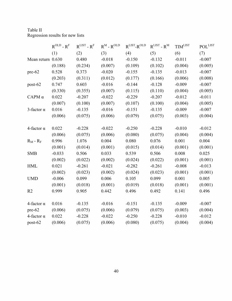
Table II Regression results for new lists ROLD - RF RLIST - RF RM - ROLD RLIST-ROLD RLIST - RM TIMLIST POLLIST (1) (2) (3) (4) (5) (6) (7) Mean return 0.630 0.480 -0.018 -0.150 -0.132 -0.011 -0.007 (0.188) (0.234) (0.007) (0.109) (0.102) (0.004) (0.005) pre-62 0.528 0.373 -0.020 -0.155 -0.135 -0.013 -0.007 (0.203) (0.311) (0.012) (0.177) (0.166) (0.006) (0.008) post-62 0.747 0.603 -0.016 -0.144 -0.128 -0.009 -0.007 (0.330) (0.355) (0.007) (0.115) (0.110) (0.004) (0.005) CAPM α 0.022 -0.207 -0.022 -0.229 -0.207 -0.012 -0.011 (0.007) (0.100) (0.007) (0.107) (0.100) (0.004) (0.005) 3-factor α 0.016 -0.135 -0.016 -0.151 -0.135 -0.009 -0.007 (0.006) (0.075) (0.006) (0.079) (0.075) (0.003) (0.004) 4-factor α 0.022 -0.228 -0.022 -0.250 -0.228 -0.010 -0.012 (0.006) (0.075) (0.006) (0.080) (0.075) (0.004) (0.004) RM - RF 0.996 1.076 0.004 0.080 0.076 0.001 0.004 (0.001) (0.014) (0.001) (0.015) (0.014) (0.001) (0.001) SMB -0.033 0.506 0.033 0.539 0.506 0.008 0.025 (0.002) (0.022) (0.002) (0.024) (0.022) (0.001) (0.001) HML 0.021 -0.261 -0.021 -0.282 -0.261 -0.008 -0.013 (0.002) (0.023) (0.002) (0.024) (0.023) (0.001) (0.001) UMD -0.006 0.099 0.006 0.105 0.099 0.001 0.005 (0.001) (0.018) (0.001) (0.019) (0.018) (0.001) (0.001) R2 0.999 0.905 0.442 0.496 0.492 0.141 0.496 4-factor α 0.016 -0.135 -0.016 -0.151 -0.135 -0.009 -0.007 pre-62 (0.006) (0.075) (0.006) (0.079) (0.075) (0.003) (0.004) 4-factor α 0.022 -0.228 -0.022 -0.250 -0.228 -0.010 -0.012 post-62 (0.006) (0.075) (0.006) (0.080) (0.075) (0.004) (0.004)

40

Table II Notes RM is the CRSP market return. RF is the t-bill portfolio return. ROLD is the return on old stock, a portfolio of stocks that have not newly appeared in CRSP in the last 36 months. RLIST is the return on new lists, a portfolio of stocks that have newly appeared in CRSP in the last 36 months. All returns are value weighted, monthly, in percent. wLIST is the portfolio weight of the market in newly listed stocks, and has average value of LISTw over the entire sample period. POLLIST is

(LIST LIST OLDt tw R R− ) and TIMLIST is ( )( )LIST LIST LIST OLD

t tw w R R− − t . The CAPM α is the intercept term from a regression on RM - RF. The three-factor α is the intercept term from a regression on the three variables of Fama and French (1993), including the excess market return, SMB (the return on small stocks minus big stocks) and the HML (the return of high B/M stocks minus low B/M stocks). The four-factor model adds UMD, a momentum factor reflecting the return of stocks with high prior year returns minus stocks with low prior year returns. Pre-1962 is prior to August 1962 (when AMEX firms enter CRSP). Post-1962 is after July 1962. The sample period is December 1929 to March 2001. Standard errors in parentheses.

41

Table III Summary Statistics for net new issues Panel A

Variable Mean t-stat on mean Std. Dev. Min Max

RLAG - RF 0.647 3.451 5.520 -28.419 38.376RNNI - RF 0.391 1.861 6.178 -31.021 35.946RM – RLAG -0.035 3.591 0.285 -2.638 2.159RPLUS – RLAG -0.201 4.070 1.456 -7.077 9.135RMINUS – RLAG 0.366 3.459 3.115 -24.036 27.328RLIST – RLAG -0.167 1.507 3.262 -22.764 22.041TIMNNI -0.013 2.752 0.140 -1.559 1.088POLNNI -0.022 3.181 0.201 -1.329 1.158TIMPLUS -0.002 1.320 0.049 -0.388 0.266POLPLUS -0.011 4.070 0.080 -0.387 0.500TIMMINUS 0.000 0.506 0.019 -0.110 0.197POLMINUS -0.003 3.459 0.025 -0.218 0.192TIMLIST -0.011 3.034 0.109 -1.398 0.939POLLIST -0.008 1.507 0.152 -1.058 1.024wNNI 0.093 60.857 0.045 0.021 0.272wPLUS 0.055 59.798 0.027 0.007 0.146wMINUS -0.008 24.805 0.009 -0.039 0.000wLIST 0.046 52.886 0.026 0.009 0.147 Panel B Correlations RLAG - RF RNNI - RF RM – RLAG TIMNNI POLNNI wNNI WPLUS WMINUS RNNI - RF 0.943 RM – RLAG 0.133 0.422 TIMNNI 0.001 0.149 0.759 POLNNI 0.188 0.496 0.891 0.381 wNNI -0.124 -0.150 -0.183 -0.204 -0.117 wPLUS -0.087 -0.116 -0.164 -0.183 -0.104 0.875 wMINUS -0.014 0.010 0.056 0.059 0.039 -0.124 -0.311 wLIST -0.121 -0.145 -0.169 -0.186 -0.110 0.877 0.598 -0.259

42

Table III Notes RM is the CRSP market return. RF is the t-bill portfolio return. RLAG is the return on a portfolio of stocks that have not newly appeared in CRSP in the last 36 months, using value weights calculated with the number of shares outstanding 36 months ago. RLIST is the return on new lists, a portfolio of stocks that have newly appeared in CRSP in the last 36 months. RPLUS is the return on shares added in the last 36 months by firms that were on CRSP 36 months ago, using value weights calculated with the number of shares that have been added. RMINUS is the return on shares subtracted in the last 36 months by firms that were on CRSP 36 months ago, using value weights calculated with the number of shares that have been subtracted. All returns are value weighted, monthly, in percent. All calculations using shares are split-adjusted. wLIST is the portfolio weight of the market in newly listed stocks, and has average value of LISTw over the entire sample period. POLLIST is ( )LIST LIST LAG

t tw R R− and TIMLIST is

( )(LIST LIST LIST LAGt tw w R R− − )t . The weights, policy returns, and timing returns are calculated

similarly for PLUS and MINUS.

43

Table IV Regression results for net new issues

--NNI-- --PLUS-- --MINUS-- --LIST-- RM – RLAG TIM POL TIM POL TIM POL TIM POL

Mean return -0.035 -0.013 -0.022 -0.002 -0.011 0.000 -0.003 -0.011 -0.008 (0.010) (0.005) (0.007) (0.002) (0.003) (0.001) (0.001) (0.004) (0.005)

pre-62 -0.042 -0.017 -0.025 -0.004 -0.013 0.000 -0.004 -0.013 -0.008 (0.016) (0.007) (0.011) (0.002) (0.003) (0.001) (0.001) (0.006) (0.008)

post-62 -0.027 -0.009 -0.018 0.000 -0.009 0.001 -0.002 -0.009 -0.007 (0.009) (0.005) (0.008) (0.003) (0.005) (0.001) (0.002) (0.004) (0.005)

CAPM α -0.041 -0.014 -0.027 -0.002 -0.013 0.000 -0.003 -0.012 -0.011 (0.010) (0.005) (0.007) (0.002) (0.003) (0.001) (0.001) (0.004) (0.005)

3-factor α -0.032 -0.010 -0.022 -0.001 -0.012 0.000 -0.002 -0.010 -0.008 (0.007) (0.004) (0.005) (0.002) (0.002) (0.001) (0.001) (0.003) (0.004)

4-factor α -0.038 -0.013 -0.025 -0.002 -0.010 0.000 -0.002 -0.010 -0.012 (0.007) (0.005) (0.005) (0.002) (0.003) (0.001) (0.001) (0.004) (0.004)

RM - RF 0.006 0.001 0.005 0.000 0.001 0.000 0.000 0.001 0.004 (0.001) (0.001) (0.001) (0.000) (0.000) (0.000) (0.000) (0.001) (0.001)

SMB 0.042 0.010 0.032 0.000 0.008 0.001 -0.001 0.008 0.025 (0.002) (0.001) (0.002) (0.000) (0.001) (0.000) (0.000) (0.001) (0.001)

HML -0.029 -0.010 -0.019 -0.002 -0.005 0.000 -0.001 -0.008 -0.013 (0.002) (0.001) (0.002) (0.000) (0.001) (0.000) (0.000) (0.001) (0.001)

UMD 0.006 0.002 0.003 0.001 -0.002 0.000 0.000 0.001 0.005 (0.002) (0.001) (0.001) (0.000) (0.001) (0.000) (0.000) (0.001) (0.001)

R2 0.432 0.134 0.467 0.068 0.182 0.055 0.072 0.142 0.498

4-factor α -0.032 -0.010 -0.022 -0.001 -0.012 0.000 -0.002 -0.010 -0.008pre-62 (0.007) (0.004) (0.005) (0.002) (0.002) (0.001) (0.001) (0.003) (0.004)4-factor α -0.038 -0.013 -0.025 -0.002 -0.010 0.000 -0.002 -0.010 -0.012post-62 (0.007) (0.005) (0.005) (0.002) (0.003) (0.001) (0.001) (0.004) (0.004)

44

Table IV Notes RM is the CRSP market return. RF is the t-bill portfolio return. RLAG is the return on a portfolio of stocks that have not newly appeared in CRSP in the last 36 months, using value weights calculated with the number of shares outstanding 36 months ago. RLIST is the return on new lists, a portfolio of stocks that have newly appeared in CRSP in the last 36 months. RPLUS is the return on shares added in the last 36 months by firms that were on CRSP 36 months ago, using value weights calculated with the number of shares that have been added. RMINUS is the return on shares subtracted in the last 36 months by firms that were on CRSP 36 months ago, using value weights calculated with the number of shares that have been subtracted. All returns are value weighted, monthly, in percent. All calculations using shares are split-adjusted. wLIST is the portfolio weight of the market in newly listed stocks, and has average value of LISTw over the entire sample period. POLLIST is ( )LIST LIST LAG

t tw R R− and TIMLIST is

( )(LIST LIST LIST LAGt tw w R R− − )t . The weights, policy returns, and timing returns are calculated

similarly for PLUS and MINUS. The CAPM α is the intercept term from a regression on RM - RF. The three-factor α is the intercept term from a regression on the three variables of Fama and French (1993), including the excess market return, SMB (the return on small stocks minus big stocks) and the HML (the return of high B/M stocks minus low B/M stocks). The four-factor model adds UMD, a momentum factor reflecting the return of stocks with high prior year returns minus stocks with low prior year returns. Pre-1962 is prior to August 1962 (when AMEX firms enter CRSP). Post-1962 is after July 1962. The sample period is December 1929 to March 2001. Standard errors in parentheses.

45

Table V Regression results for net new issues

Mean return CAPM α 3-factor α 4-factor α

SECTORTIMPLUS 0.000 0.000 0.000 0.001 (0.000) (0.000) (0.000) (0.000)SELECTTIMPLUS -0.003 -0.002 -0.001 -0.003 (0.002) (0.002) (0.002) (0.002)SECTORPOLPLUS -0.001 -0.001 -0.001 0.000 (0.001) (0.001) (0.001) (0.001)SELECTPOLPLUS -0.010 -0.012 -0.011 -0.010 (0.002) (0.002) (0.002) (0.002) SECTORTIMMINUS 0.000 0.000 0.000 0.000 (0.000) (0.000) (0.000) (0.000)SELECTTIMMINUS 0.000 0.000 0.000 0.000 (0.001) (0.001) (0.001) (0.001)SECTORPOLMINUS -0.001 -0.001 0.000 0.000 (0.000) (0.000) (0.000) (0.000)SELECTPOLMINUS -0.002 -0.002 -0.002 -0.002 (0.001) (0.001) (0.001) (0.001) SECTORTIMLIST -0.003 -0.003 -0.002 -0.002 (0.001) (0.001) (0.001) (0.001)SELECTTIMLIST -0.007 -0.008 -0.006 -0.007 (0.003) (0.003) (0.003) (0.003)SECTORPOLLIST -0.001 -0.001 -0.001 -0.002 (0.002) (0.002) (0.002) (0.002)SELECTPOLLIST -0.007 -0.010 -0.006 -0.010 (0.004) (0.004) (0.004) (0.004)

46

Table V Notes Table V is based on 26 portfolios. The definition of LAG, LIST, PLUS, and MINUS are as in Table IV. Every year in July, I break all stocks in CRSP into five groups according to market capitalization and five groups according to book value, using book data from an updated version of Davis, Fama, and French (2000). The quintiles use NYSE breakpoints, the sorting is done in July of each year based on B/M on the previous December and market equity in June. In addition to the 25 portfolios defined by these quintiles, a 26th portfolio consists of all CRSP firms without an available B/M number. vLAG,i is the fraction of the market capitalization of portfolio LAG that is invested in sector i. vLIST,i is the fraction of the market capitalization of portfolio LIST that is invested in sector i. For new

lists: ( ) ( )26

, ,

1

LIST LIST LIST LIST i LAG i LAG it t t t t t

i

SECTORTIM w w v v R=

, = − − ∑ ,

( )26

, ,

1

LIST LIST LIST LIST LIST i LAG it t t t t t

i

LECTTIM w w R v R=

SE = − − ∑ ,

( )26

, , ,

1

LIST LIST LIST i LAG i LAG it t t t t

i

TORPOL w v v R=

= − ∑SEC ,

26, ,

1

LIST LIST LIST LIST i LAG it t t t t

i

ECTPOL w R v R=

= − ∑SEL

and similarly for PLUS and MINUS. The sample period is December 1929 to March 2001. Standard errors in parentheses.

47

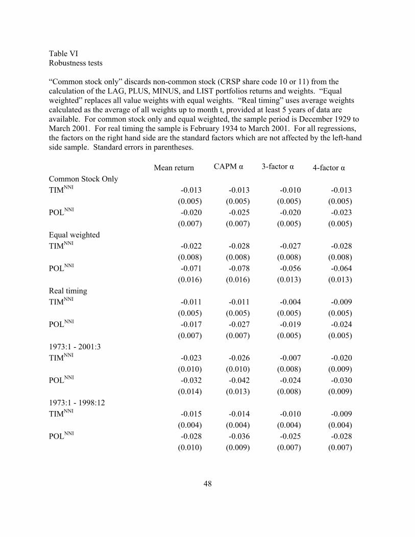
Table VI Robustness tests “Common stock only” discards non-common stock (CRSP share code 10 or 11) from the calculation of the LAG, PLUS, MINUS, and LIST portfolios returns and weights. “Equal weighted” replaces all value weights with equal weights. “Real timing” uses average weights calculated as the average of all weights up to month t, provided at least 5 years of data are available. For common stock only and equal weighted, the sample period is December 1929 to March 2001. For real timing the sample is February 1934 to March 2001. For all regressions, the factors on the right hand side are the standard factors which are not affected by the left-hand side sample. Standard errors in parentheses.

Mean return CAPM α 3-factor α 4-factor α Common Stock Only TIMNNI -0.013 -0.013 -0.010 -0.013 (0.005) (0.005) (0.005) (0.005)POLNNI -0.020 -0.025 -0.020 -0.023 (0.007) (0.007) (0.005) (0.005)Equal weighted TIMNNI -0.022 -0.028 -0.027 -0.028 (0.008) (0.008) (0.008) (0.008)POLNNI -0.071 -0.078 -0.056 -0.064 (0.016) (0.016) (0.013) (0.013)Real timing TIMNNI -0.011 -0.011 -0.004 -0.009 (0.005) (0.005) (0.005) (0.005)POLNNI -0.017 -0.027 -0.019 -0.024 (0.007) (0.007) (0.005) (0.005)1973:1 - 2001:3 TIMNNI -0.023 -0.026 -0.007 -0.020 (0.010) (0.010) (0.008) (0.009)POLNNI -0.032 -0.042 -0.024 -0.030 (0.014) (0.013) (0.008) (0.009)1973:1 - 1998:12 TIMNNI -0.015 -0.014 -0.010 -0.009 (0.004) (0.004) (0.004) (0.004)POLNNI -0.028 -0.036 -0.025 -0.028 (0.010) (0.009) (0.007) (0.007)

48

Table VII Predictive power of portfolio weights for portfolio returns Forecasting regressions of differential returns on portfolio weights. RLAG is the return on a portfolio of stocks that have not newly appeared in CRSP in the last 36 months, using value weights calculated with the number of shares outstanding 36 months ago. RLIST is the return on new lists, a portfolio of stocks that have newly appeared in CRSP in the last 36 months. RPLUS is the return on shares added in the last 36 months by firms that were on CRSP 36 months ago, using value weights calculated with the number of shares that have been added. RMINUS is the return on shares subtracted in the last 36 months by firms that were on CRSP 36 months ago, using value weights calculated with the number of shares that have been subtracted. All returns are value weighted, monthly, in percent. All calculations using shares are split-adjusted. wLIST is the portfolio weight of the market in newly listed stocks. The sample period is December 1929 to March 2001. Standard errors in parentheses. RNNI – RLAG RPLUS – RLAG RMINUS – RLAG RLIST – RLAG Constant 0.244 0.306 -0.046 -0.018 0.555 0.511 0.244 0.306 (0.161) (0.167) (0.114) (0.118) (0.243) (0.252) (0.161) (0.167)wNNI -5.363 -1.668 -2.033 -5.363 (1.558) (1.096) (2.347) (1.558) wPLUS -5.159 -2.249 8.578 -5.159 (3.321) (2.338) (4.992) (3.321)wMINUS 6.078 2.714 2.218 6.078 (7.827) (5.511) (11.765) (7.827)wLIST -4.981 -0.836 -12.851 -4.981 (3.405) (2.397) (5.118) (3.405) R2 0.014 0.016 0.003 0.004 0.001 0.008 0.014 0.016 P-values: wPLUS= wMINUS= wLIST

=0 0.003 0.374 0.089 0.003 wPLUS= wMINUS= wLIST 0.327 0.668 0.056 0.327

49

Table VIII Predictive power of portfolio weights for aggregate returns Forecasting regressions where the dependent variable, RM - RF , is the excess return on the CRSP value weighted market. wLIST is the portfolio weight of the market in newly listed stocks, and similarly for PLUS and MINUS. P/D is the ratio of current price to past year dividends for the S&P Composite index. P/E10 is the market ratio of current price to average earnings per share over the past 10 years, for the S&P Composite index. Billyield is the t-bill yield. Share is the equity share over the past year, calculated as gross equity issues divided by gross equity issues plus gross debt issues. For monthly regressions the sample period is December 1929 to March 2001. For annual regressions the sample period is 1927 to 1995. Standard errors in parentheses. Annual Annual Constant 1.461 2.099 2.387 2.661 2.268 2.516 32.130 55.156 (0.454) (0.523) (0.523) (0.555) (0.505) (0.539) (5.780) (8.876)wNNI -15.349 -13.610 (4.411) (4.645) wLIST -26.905 -24.052 -245.673 -132.312 (7.622) (8.152) (96.535) (97.567)P/D -0.016 0.000 0.000 (0.014) (0.015) (0.015) P/E10 -0.062 -0.026 -0.022 -1.642 (0.026) (0.029) (0.029) (0.512)Billyield -10.666 -12.044 -8.680 -9.093 -10.640 -10.777 -67.817 (5.812) (5.671) (5.803) (5.735) (5.773) (5.662) (62.336)Share -64.024 -69.090 (21.734) (21.154) R2 0.007 0.011 0.020 0.021 0.021 0.021 0.239 0.351

50

Table IX Properties of substitute portfolios RM is the CRSP market return. RF is the t-bill portfolio return. ROLD is the value weighted return on a portfolio of stocks that have not newly appeared in CRSP in the last 36 months. RLAG is the return on a portfolio of stocks that have not newly appeared in CRSP in the last 36 months, using value weights calculated with the number of shares outstanding 36 months ago. wLIST is the portfolio weight of the market in newly listed stocks. wNNI is the portfolio weight of the market in newly listed stocks, plus shares added in the last 36 months by firms which were on CRSP 36 months ago, minus shares subtracted in the last 36 months by firms which were on CRSP 36 months ago. SBILLLIST = (1- wLIST)(ROLD -RF). SBILLNNI = (1- wNNI)(RLAG -RF). SCASHLIST = (1- wLIST)ROLD - RF. SBILLNNI = (1- wNNI)RLAG - RF. The CAPM α is the intercept term from a regression on RM - RF. The three-factor α is the intercept term from a regression on the three variables of Fama and French (1993), including the excess market return, SMB (the return on small stocks minus big stocks) and the HML (the return of high B/M stocks minus low B/M stocks). The four-factor model adds UMD, a momentum factor reflecting the return of stocks with high prior year returns minus stocks with low prior year returns. The sample period is December 1929 to March 2001. Standard errors in parentheses. RM- RF ROLD -RF RLAG -RF SBILLLIST

SBILLNNI SCASHLIST SCASHNNI

Mean return 0.612 0.630 0.647 0.618 0.617 0.603 0.586Std dev 5.565 5.530 5.520 5.230 4.910 5.231 4.913SR 0.110 0.114 0.117 0.118 0.126 0.115 0.119 CAPM α 0.022 0.041 0.044 0.080 0.029 0.048 (0.007) (0.010) (0.010) (0.015) (0.010) (0.015)3-factor α 0.016 0.032 0.037 0.071 0.021 0.039 (0.002) (0.007) (0.009) (0.015) (0.009) (0.015)4-factor α 0.022 0.038 0.029 0.048 0.014 0.017 (0.006) (0.007) (0.009) (0.015) (0.009) (0.015)

51

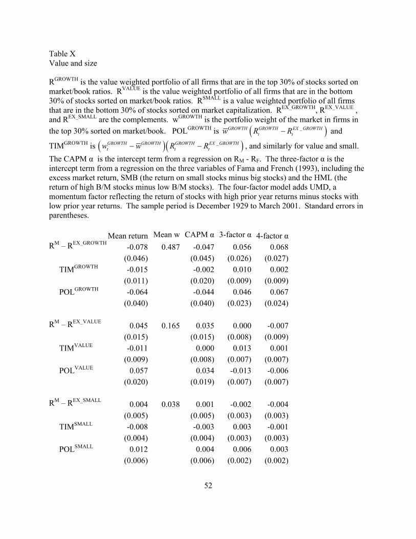
Table X Value and size RGROWTH is the value weighted portfolio of all firms that are in the top 30% of stocks sorted on market/book ratios. RVALUE is the value weighted portfolio of all firms that are in the bottom 30% of stocks sorted on market/book ratios. RSMALL is a value weighted portfolio of all firms that are in the bottom 30% of stocks sorted on market capitalization. REX_GROWTH, REX_VALUE , and REX_SMALL are the complements. wGROWTH is the portfolio weight of the market in firms in the top 30% sorted on market/book. POLGROWTH is ( )_GROWTH GROWTH EX GROWTH

t tw R R− and

TIMGROWTH is ( ) , and similarly for value and small. The CAPM α is the intercept term from a regression on RM - RF. The three-factor α is the intercept term from a regression on the three variables of Fama and French (1993), including the excess market return, SMB (the return on small stocks minus big stocks) and the HML (the return of high B/M stocks minus low B/M stocks). The four-factor model adds UMD, a momentum factor reflecting the return of stocks with high prior year returns minus stocks with low prior year returns. The sample period is December 1929 to March 2001. Standard errors in parentheses.

( _GROWTH GROWTH GROWTH EX GROWTHt t tw w R R− − )

Mean return Mean w CAPM α 3-factor α 4-factor α

RM – REX_GROWTH -0.078 0.487 -0.047 0.056 0.068 (0.046) (0.045) (0.026) (0.027) TIMGROWTH -0.015 -0.002 0.010 0.002 (0.011) (0.020) (0.009) (0.009) POLGROWTH -0.064 -0.044 0.046 0.067 (0.040) (0.040) (0.023) (0.024) RM – REX_VALUE 0.045 0.165 0.035 0.000 -0.007 (0.015) (0.015) (0.008) (0.009) TIMVALUE -0.011 0.000 0.013 0.001 (0.009) (0.008) (0.007) (0.007) POLVALUE 0.057 0.034 -0.013 -0.006 (0.020) (0.019) (0.007) (0.007) RM – REX_SMALL 0.004 0.038 0.001 -0.002 -0.004 (0.005) (0.005) (0.003) (0.003) TIMSMALL -0.008 -0.003 0.003 -0.001 (0.004) (0.004) (0.003) (0.003) POLSMALL 0.012 0.004 0.006 0.003 (0.006) (0.006) (0.002) (0.002)

52

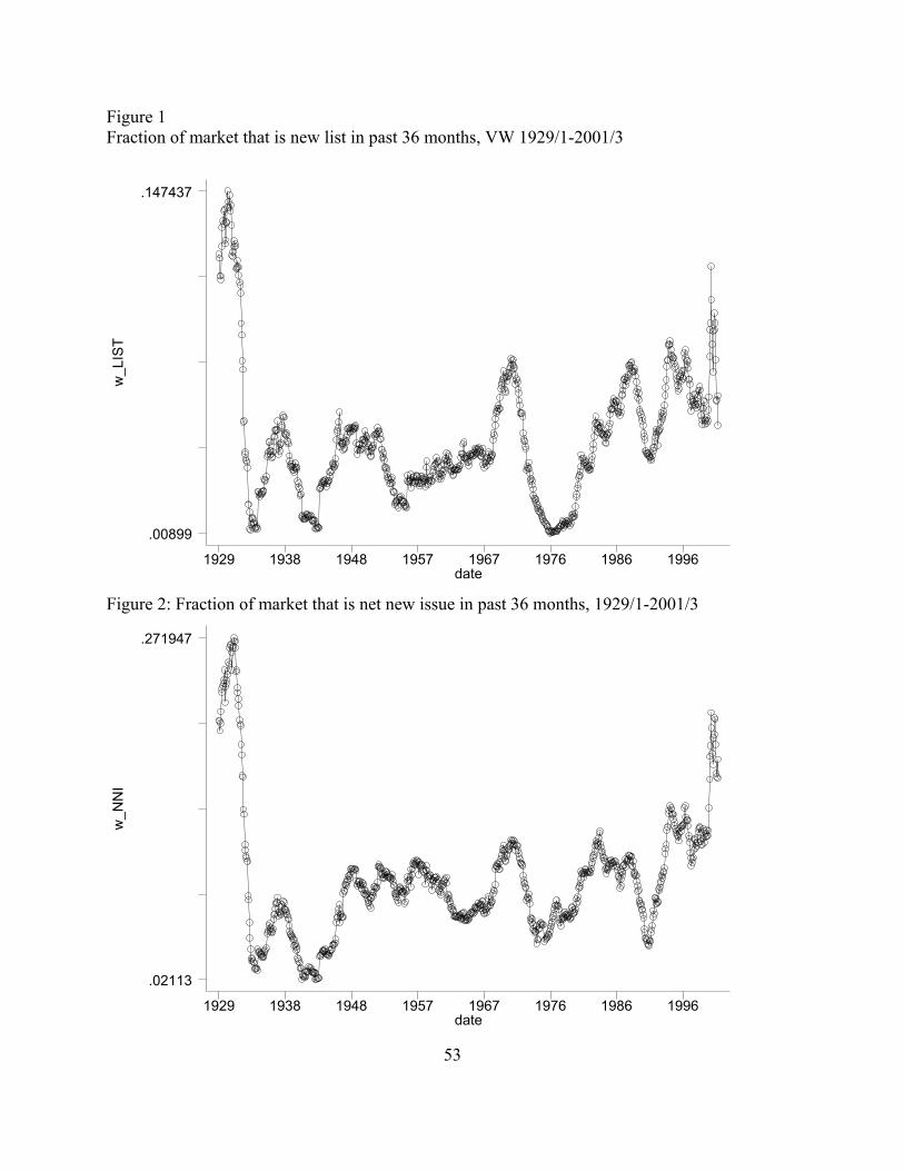
Figure 1 Fraction of market that is new list in past 36 months, VW 1929/1-2001/3

w_L

IST

date1929 1938 1948 1957 1967 1976 1986 1996

.00899

.147437

Figure 2: Fraction of market that is net new issue in past 36 months, 1929/1-2001/3

53

w_N

NI

date1929 1938 1948 1957 1967 1976 1986 1996

.02113

.271947

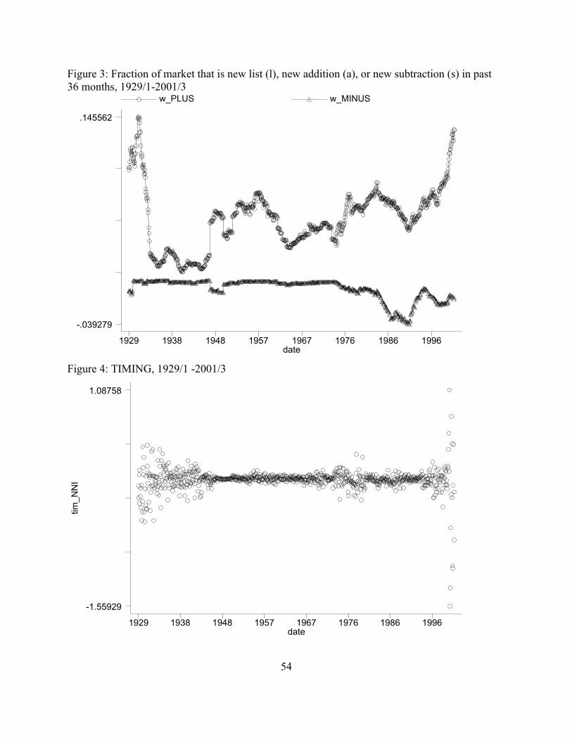
Figure 3: Fraction of market that is new list (l), new addition (a), or new subtraction (s) in past 36 months, 1929/1-2001/3

date

w_PLUS w_MINUS

1929 1938 1948 1957 1967 1976 1986 1996

-.039279

.145562

Figure 4: TIMING, 1929/1 -2001/3

tim_N

NI

date1929 1938 1948 1957 1967 1976 1986 1996

-1.55929

1.08758

54

evaluating value weighting: corporate events and market timing · evaluating value weighting:...

Documents