Essays in Information Asymmetry, Information Acquisition, Corporate

Governance, Capital Structure, and Financial Markets

by

Lei Gao

(Under the direction of Jeffry M. Netter)

Abstract

Information is a set of data or knowledge about a specific topic. Information has its

economic value because it facilitates individuals to make strategic choices that yield higher

expected utility than they would obtain in the absence of information. Most commonly in

finance research, information asymmetries are studied in the context of agency problems,

where the separation of ownership and controls brings in conflicts between the management

and the shareholders. In financial markets, firms’ public information, private information,

and the asymmetry between them play a crucial role in security issuing decisions, corpo-

rate capital structure decisions, and investors investing decisions. My research investigates

the interaction between information environment, corporate governance, corporate financing

decisions, and investors’ trading behavior.

The first essay of my dissertation examines pecking order theory and static trade off

theory of capital structure with the natural experiment of SOX. SOX is the most important

response to a series of high profile accounting scandals. It mandates better quality financial

reports and more independent board. It could change firms’ information environment and

management career risk. I find that firms in general dropped leverage after SOX. Firms

with larger information asymmetry ex ante dropped leverage more, and firms with more

entrenched managers dropped leverage more. Managers have incentives to use leverage less

than the optimal level, which is consistent with static trade-off theory and management

entrenchment hypothesis.

The second essay directly examines the empirical association between information acqui-

sition and investor trading. It is often assumed that investors will adjust their portfolio when

there is new information. With the availability of internet search volume, we could measure

how intensive the investor’s information acquisition is. We find that doubling abnormal search

intensity is associated with about a 9% increase in abnormal trading volume. The positive

volume-search association holds for both buyer- and seller-initiated trades, and is greater i)

for large trades than for small trades, ii) when search from local investors is more intensive,

and iii) during earnings announcement period. These results are consistent with an increase

in disagreement triggered by information acquisition.

Index words: Information Asymmetry, Information Acquisition, Agency Cost,Corporate Governance, Sarbanes-Oxley Act, Capital Structure,Financial Markets

Essays in Information Asymmetry, Information Acquisition, Corporate

Governance, Capital Structure, and Financial Markets

by

Lei Gao

B.S., Peking University, 2000

M.S., Michigan State University, 2006

A Thesis Submitted to the Graduate Faculty

of The University of Georgia in Partial Fulfillment

of the

Requirements for the Degree

Doctor of Philosophy

Athens, Georgia

2012

c⃝ 2012

Lei Gao

All Rights Reserved

Essays in Information Asymmetry, Information Acquisition, Corporate

Governance, Capital Structure, and Financial Markets

by

Lei Gao

Approved:

Major Professor: Jeffry M. Netter

Committee: Annette B. Poulsen

Tao Shu

Electronic Version Approved:

Maureen Grasso

Dean of the Graduate School

The University of Georgia

May 2012

Dedication

To my wife Lily and daughter Annie, without your endless love and support this would never

have been possible.

To my parents for investing their entire lives in ensuring the success of their children.

iv

Acknowledgments

This work could never have been accomplished without the unflinching support from those

I am honored to know and work with over the past five years.

First and foremost I owe my deepest gratitude to my advisor, Dr. Jeffry Netter, whose

encouragement, guidance and support from the initial to the final level enabled me to develop

a deep understanding of the subject. I would like to thank him for taking me as his Ph.D.

student and continuously encouraging me and teaching me to do high quality research and

teaching throughout my doctoral studies. He taught me innumerable lessons and insights

on the working of academic research. He guided me to focus on economic meaning instead

of numbers. As the Editor of Journal of Corporate Finance, Dr. Netter offers me precious

opportunities to learn the process of publication and learn how to evaluate research for his

prestigious journal. I am indebted to him always.

I would like to thank two of my committee members, Dr. Annette Poulsen and Dr. Tao

Shu for all the support and guidance throughout the period of my graduate study at the

University of Georgia and in the course of preparing this dissertation. I appreciate greatly

their continuous encouragement, insightful comments, even detailed instructions on writing

and presenting.

I would like to acknowledge Dr. Eric Yeung and Dr. Oliver Li for all their guidance and

collaboration on the research work related to the third chapter of this dissertation. I am

deeply grateful for their immense contributions of time, ideas and effort in the project,

which makes my PhD experience more productive and stimulating.

I also wish to express my gratitude to the faculty members of the Department of Banking

and Finance at the University of Georgia for their constructive suggestions and insightful

comments which lead to a much improved version of my dissertation.

v

vi

I would like to thank my fellow Ph.D. students for being great colleagues and great friends.

I am very grateful for the friendship.

I am also extremely grateful for the love and support that I have received from my parents.

Last, but by no means least, I would like to thank my wife Lily and my daughter Annie.

Your love and support through the last five years has made all of this possible. Thank you!

Table of Contents

Page

Acknowledgments . . . . . . . . . . . . . . . . . . . . . . . . . . . . . . . . . v

List of Figures . . . . . . . . . . . . . . . . . . . . . . . . . . . . . . . . . . . viii

List of Tables . . . . . . . . . . . . . . . . . . . . . . . . . . . . . . . . . . . ix

Chapter

1 Introduction . . . . . . . . . . . . . . . . . . . . . . . . . . . . . . . . 1

2 Information Asymmetry, Management Entrenchment, and Cap-

ital Structure: Evidence from the Sarbanes-Oxley Act of 2002 4

2.1 Introduction . . . . . . . . . . . . . . . . . . . . . . . . . . . . 4

2.2 Literature Review and Hypotheses Development . . . . . 8

2.3 Data . . . . . . . . . . . . . . . . . . . . . . . . . . . . . . . . . 14

2.4 Results and Discussions . . . . . . . . . . . . . . . . . . . . . 23

2.5 Conclusion and Discussions . . . . . . . . . . . . . . . . . . . 30

2.6 References . . . . . . . . . . . . . . . . . . . . . . . . . . . . . 32

3 Information Acquisition and Investor Trading: Daily Analysis . 52

3.1 Introduction . . . . . . . . . . . . . . . . . . . . . . . . . . . . 52

3.2 Literature, Theoretical Framework and Hypotheses . . . 57

3.3 Data and Research Design . . . . . . . . . . . . . . . . . . . . 63

3.4 Results . . . . . . . . . . . . . . . . . . . . . . . . . . . . . . . 68

3.5 Summary and Conclusion . . . . . . . . . . . . . . . . . . . . . 77

3.6 References . . . . . . . . . . . . . . . . . . . . . . . . . . . . . 78

vii

List of Figures

2.1 U.S. public firms’ capital structure from 1982 to 2006 . . . . . . . . . . . . . 49

2.2 U.S. public firms’ Marginal Taxes from 1982 to 2006 . . . . . . . . . . . . . . 50

2.3 Dow Jones Industrial Average between 1997 and 2006 . . . . . . . . . . . . . 50

2.4 3-Month T-Bill, AAA bond, and BAA bond yield between 1998 and 2006 . . 51

viii

List of Tables

2.1 Descriptive Statistics . . . . . . . . . . . . . . . . . . . . . . . . . . . . . . . 38

2.2 Long-run capital structure Changes . . . . . . . . . . . . . . . . . . . . . . . 39

2.3 Capital Structure changes by industry around the passage of SOX . . . . . . 40

2.4 Correlation Table . . . . . . . . . . . . . . . . . . . . . . . . . . . . . . . . . 41

2.5 Leverage before and after the SOX Act . . . . . . . . . . . . . . . . . . . . . 43

2.6 Regressions of Leverage on SOX Dummy and control variables . . . . . . . . 44

2.7 Regression of Market leverage on different information asymmetry measures 45

2.8 Regressions of Leverage Changes on Different governance index . . . . . . . . 46

2.9 Regressions of Market leverage on different external governance measures . . 47

2.10 Control Groups capital structure changes around the passage of SOX . . . . 48

2.11 U.S. Control Groups capital structure changes . . . . . . . . . . . . . . . . . 48

3.1 Descriptive Statistics . . . . . . . . . . . . . . . . . . . . . . . . . . . . . . . 82

3.2 Correlation Table . . . . . . . . . . . . . . . . . . . . . . . . . . . . . . . . . 83

3.3 Regressions of Abnormal Trading Volumes . . . . . . . . . . . . . . . . . . . 85

3.4 Regression of Abnormal Trading Volume for Different Trade Size Categories 86

3.5 Regressions of Intra-day Abnormal Volatility of Trade Size . . . . . . . . . . 89

3.6 Impact of Accruals, Earning Announcement, and Local Ticker Search on

Abnormal Trading Volume . . . . . . . . . . . . . . . . . . . . . . . . . . . . 90

3.7 Impact of Ticker Search on Directional Abnormal Trading Volumes . . . . . 91

3.8 Search Intensity, Directional Abnormal Net Buy, and Future Returns . . . . 94

ix

Chapter 1

Introduction

Information is a set of data or knowledge about a specific topic. Information has its economic

value because it facilitates individuals to make strategic choices that yield higher expected

utility than they would obtain in the absence of information. Information asymmetry studies

the decision in transactions that one party has more or better information than the other.

Some transactions could go awry because of the imbalance in power. Examples are the

adverse selection problem and the moral hazard problem. Adverse selection theory stems

from Akerlof’s “The Market for Lemons”, and it predicts that “bad” results occur when

buyers and sellers have different information set. Moral hazard refers to a situation that one

party makes a decision, while the other party bears the risk. As a consequence, the party

that makes decisions without taking corresponding risks may behave inappropriately.

Most commonly in finance research, information asymmetries are studied in the context of

agency problems, where the separation of ownership and controls brings in conflicts between

the management and the shareholders. In financial markets, firms’ public information, pri-

vate information, and the asymmetry between them play a crucial role in security issuing

decisions, corporate capital structure decisions, and investors investing decisions. Corporate

regulation laws designed for purposes might have some unintended consequences when they

have universal requirements and change the firms’ information environment.

My dissertation research investigates the interaction between information environment,

corporate governance, corporate financing decisions, and investors’ trading behavior.

Due to several high profile public firm accounting scandals in early 2000s, financial

markets faced a big challenge of attracting investors. Because the information asymmetry

1

2

between insiders and investors is threatening the viability of financial markets, the Sarbanes-

Oxley Act (SOX) was passed to improve the financial reports’ quality, and thus to gain

investors’ confidence. The passage of SOX provides a natural experiment to test the capital

structure theories derived from the information asymmetry problems.

On the one hand, managers make financing decisions based on his perception of informa-

tion asymmetry. On the other hand, investors try to become informed through information

acquisition. Information goods are non-rivalrous and non-excludable. When there is new

information released on a firm or the overall economic environment, the divergent under-

standing of the same information could lead to trade transactions. However, the relationship

of between information acquisition, information intensity, and investors’ trading behavior

has not been empirically tested, partly due to the lack of a proxy for information acquisition

or information intensity. My research aims to critically examine how information plays an

important role in both corporate financing decisions and investor trading behaviors.

The first essay of my dissertation examines pecking order theory and static trade off

theory of capital structure with the natural experiment of SOX. SOX is the most important

response to a series of high profile accounting scandals (e.g. Enron and WorldCom). It

mandates better quality financial reports and more independent board. Critics noted a “One-

Size-Fits-All” policy might not be optimal. Empirically, it provides us a natural experiment

to test theories of capital structure. And my study also contributes to the literatures of the

unintended consequences of SOX.

I find that firms in general dropped leverage after SOX. Firms with larger informa-

tion asymmetry ex ante dropped leverage more than firms with smaller information asym-

metry, and firms with more entrenched managers dropped leverage more than firms with less

entrenched managers. Managers have incentives to use leverage less than the optimal level,

which is consistent with static trade-off theory and management entrenchment hypothesis.

The second essay directly examines the empirical association between information acqui-

sition and investor trading. It is often assumed that investors will adjust their portfolio when

3

there is new information. Investors choose to become informed through information acquisi-

tion and the cost of acquiring information is compensated by taking positions in risky assets

and expecting positive abnormal returns. Information acquisition likely yields disagreement

among investors and spurs trading. Despite the theoretical advancement, the association

between information acquisition and trading activities has seldom been empirically tested

due to the fact that the proxy for information acquisition is largely not observable.

How is information revealed and distributed? With the developing of technology, it is

becoming easier for people to acquire information. For hundreds of years, people read news-

papers to get information. When radio and TV were invented, people started to get more

timely information. In the internet era, vast information is so easy to get that people call it

“information explosion” era. Internet search engines provide good entrances to acquire infor-

mation. If we could know what people search for and how intensive the searches are, we could

learn the intensity of information acquisition. Out of all the web search engines, Google has

around 70% market share. With the availability of internet search volume, we could measure

how intensive the investor’s information acquisition is. It is possible to examine the empirical

association between information acquisition and daily abnormal trading activities.

We find that doubling abnormal search intensity is associated with about a 9% increase in

abnormal trading volume. The positive volume-search association holds for both buyer- and

seller-initiated trades, and is greater i) for large trades than for small trades, ii) when search

from local investors is more intensive, and iii) during earnings announcement period. These

results are consistent with an increase in disagreement triggered by information acquisition.

Chapter 2

Information Asymmetry, Management Entrenchment, and Capital

Structure: Evidence from the Sarbanes-Oxley Act of 2002

2.1 Introduction

As a “one-size-fits-all” law, the Sarbanes-Oxley Act (SOX) of 2002 was designed to improve

information transparency and investors’ confidence in firms’ financial reports. It has been

praised widely by regulators and regarded as “the most far-reaching reform of American

business practices since the time of Franklin D. Roosevelt”1. Academic researchers have

found evidence of the benefits of SOX; these include corporate transparency improvements

(Arping and Sautner (2010)) and positive abnormal returns for less compliant firms after the

announcement of SOX (Chhaochharia and Grinstein (2007)). On the other hand, researchers

have also identified some unintended consequences of SOX, such as its negative effect on firm

value (Zhang (2007)), shifted supply and demand for directors (Linck, Netter, and Yang

(2009)), changed compensation structure (Carter, Lynch, and Zechman (2009)), reduced

investment (Kang, Liu and Qi (2010)), and smaller international companies’ moving to stock

exchanges in the United Kingdom rather than trading in the United States (Piotroski and

Srinivasan (2008)).

In this paper, I examine the effects of SOX on capital structure, a subject that has not

been studied in the literature. SOX can affect capital structure through its effect on corporate

1 See http://nytimes.com/. Also see former Federal Reserve Chairman AlanGreenspan praised the Sarbanes-Oxley Act: “I am surprised that the Sarbanes-OxleyAct, so rapidly developed and enacted, has functioned as well as it has...” Seehttp://www.federalreserve.gov/boarddocs/speeches/2005/20050515/default.htm. SEC ChairmanChristopher Cox stated in 2007: “Sarbanes-Oxley helped restore trust in U.S. markets byincreasing accountability, speeding up reporting, and making audits more independent.” Seehttp://www.usatoday.com.

4

5

information transparency. As stated by the pecking order theory, firms prefer internal funding

over external funding and prefer debt funding over equity funding because of the adverse

selection induced by information asymmetry. On the one hand, when information asymmetry

is reduced, the disadvantage of equity financing relative to debt financing is also reduced,

making firms more willing to use equity funding relative to debt financing. Thus, we should

expect leverage to decrease a firm’ information asymmetry is reduced. Since SOX requires

public firms to release reliable financial reports and improve information transparency, we

should expect a leverage reduction after the passage of SOX according to the pecking order

theory. On the other hand, less information asymmetry lead to lower cost of debt and weaker

debt covenants. Firms’ leverage might increase post SOX.

SOX could also affect capital structure through its impact on the incentives of corporate

managers. Trade-off theory, another major theory of capital structure, suggests that capital

structure is determined by the trade-off between the costs and benefits based on a wide range

of factors. On the one hand, management entrenchment theory suggests that managers are

reluctant to issue debt because financial distress can lead to salary cuts, discipline, or even

possible job losses (see Zwiebel (1996), Morellec (2004), and Berk, Stanton and Zechner

(2010)). Since SOX was designed to regulate executives of public firms, especially those who

are most responsible for the financial reports, such as CEOs and CFOs, SOX can increase

the career risk of corporate executives (see Wang (2010), and Linck, Netter, and Yang (2009)

among others). Job security is one of the most important determinants of human happiness

(Clark and Oswald 1994; Di Tella, MacCulloch and Oswald 2001; Helliwell 2003);2 when

SOX adds to managers’ career risk and upsets the balance of their trade-off, according to

the hypotheses of management entrenchment theory, managers have sufficient motivation to

2Clark and Oswald (1994) report large well-being reductions from being unemployed. Simi-larly, Di Tella, MacCulloch, and Oswald (2001) find that a 1% increase in the unemployment ratedecreases overall happiness 66% more than a 1% increase in the inflation rate. Furthermore, Helli-well (2003) finds that job loss is outranked only by divorce in its detrimental effect on happiness inthe events he studies. Job loss even outranks the death of a spouse. This literature suggests thatmanagers would treat the newly added career risk from SOX very seriously.

6

offset their career risk by reducing the leverage level. On the other hand, since SOX requires

high quality financial reports, reports that require signature of both CEO and CFO and

are authenticated by external auditors, firms who used to hide excessive debts could no

longer hide as much. Firms need to unload debts to avoid financial distress. And firms with

more entrenched managers may get rid of more debts even though the new debt level is not

optimal.

The present study examines a large panel of over 7,000 U.S. corporations and finds that

firms reduced their leverage by 8.6% (market leverage) or 2.4% (book leverage) on a uni-

variate basis after SOX went into effect, which is effectively around 25% (market leverage)

or 6% (book leverage) relative to the average leverage of the whole sample during the 8

years around SOX. At the industry level, 80% of industries reduced their book leverage and

all the industries reduced their market leverage post SOX. The changes are both statisti-

cally and economically significant. The effects are robust in multivariate regressions. Firms

reduced their market leverage by 4.5% (effectively around 15%) in a multivariate regression

controlling for market-to-book and other factors.

To examine the explanation based on the pecking order theory, I look at the change

in leverage across firms with different information asymmetry levels. Using the proxies of

information asymmetry including analyst coverage (Chang, Dasgupta and Hilary (2006)),

idiosyncratic volatility, and probability of informed trades (PIN, Easley, Kiefer and O’Hara

(1997), and Adjusted PIN, Duarte and Young (2009)), I find that, consistent with the pecking

order theory, firms with fewer analysts following them decreased leverage significantly more

than firms with more analysts, and firms with higher idiosyncratic volatility reduced leverage

significantly more than firms with lower idiosyncratic volatility. I also find that firms with

a higher PIN (more information asymmetry) reduced leverage significantly more than firms

with a lower PIN. Another unique information asymmetry proxy is information acquisition

volatility (SVIVol), which is based on investor’s ticker search behaviors on Google (See Da,

Engelberg, and Gao (2011)).

7

I further examine whether trade-off theory also contributes to the reduced leverage.

Specifically, I first examine whether firms with managers who are more sensitive to reputa-

tion or job loss dropped leverage significantly more than their counterparts. I use industry

concentration of a firm as a proxy for managerial sensitivity to job loss; since it is harder

for a manager who works in a highly concentrated industry to find a comparable job when

being fired, he or she is naturally more sensitive to career risk. Consistent with the trade-off

theory, I find that firms in highly concentrated industries reduced leverage by 25% more than

their counterparts on a univariate basis. This result is robust in multivariate analyses. I also

examine whether firms with managers who are more entrenched reduced leverage much more

than their counterparts. I use institutional ownership, governance index, and entrenchment

index as proxies for managerial entrenchment and find that firms with low institutional own-

ership, higher governance index (more entrenchment), and higher entrenchment index (more

entrenchment) reduced leverage by at least 30% more than their counterparts.

As the first study to look at the impact of SOX on capital structure, my work contributes

to both the capital structure literature and the SOX literature. My study tests both the

information asymmetry and static trade-off theories on capital structure. It reveals that firms

with higher information asymmetry ex ante reduced leverage more after the passage of SOX.

My study investigates the interaction of industry concentration, institutional ownership,

and internal corporate governance with capital structure. I find that executive preference

and corporate governance could impact firms’ observed capital structure significantly when

firms face regulation shocks like SOX. My study suggests trade-off theory could explain the

observed capital structure changes.

The rest of the present chapter is organized as follows. Section 2.2 presents a literature

review and the development of the main hypotheses. Section 2.3 describes the sample data

and empirical methods. Section 2.4 presents the results and analysis. Section 2.5 provides

the conclusion and discussion.

8

2.2 Literature Review and Hypotheses Development

SOX was a consequence of a series of high profile accounting scandals, however, it is regarded

as an extra burden for those firms who already complied the rules. When considering SOX

as a regulation shock to test capital structure theories explaining observed capital structure

changes, I focus on pecking order theory and trade-off theory.

Pecking order theory stems from Akerlof’s (1970)’s “Lemon” theory - buyers will discount

the price they are willing to pay when a seller has private information about the value of

a good, due to adverse selection. Myers (1984) and Myers and Majluf (1984) extended the

theory to include capital structure. In this paper, I use the terms pecking order theory and

information asymmetry theory interchangeably because pecking order is implied by informa-

tion asymmetry. According to pecking order theory, firms will prefer internal funding over

external funding and debt financing over equity financing. The more information asymmetry

associated with a firm, the less likely it will use equity financing relative to debt financing.

No doubt, SOX has increased financial report quality; and thus has improved information

transparency. It is natural to assume that information asymmetry has been reduced since the

passage of SOX. According to the original pecking order, this reduced information asymmetry

should help to partially alleviate adverse selection and make firms more willing to use equity

relative to debt to fund their projects. Therefore we should expect a leverage decrease as a

result of SOX according to pecking order theory.

Figure 2.1 shows the market leverage and book leverage of U.S. firms over the 25 years

from 1982 to 2006. There is no clear pattern of the capital structure of US public firms over

this long period except that the market leverage is decreasing on average. There are several

sharp short-term changes. The most recent one happened around year 2002, which coincides

with the passage of the influencing law - SOX. This plummet is my interest of research.

Trade-off theory explains capital structure as a trade-off between the benefits and the

costs of debt. Jensen and Meckling (1976) and Jensen (1986) regard debt as a monitoring

tool to discipline managers and mitigate agency problems of free cash flow. Later the cost

9

of debt in the trade-off was extended from the arguably small direct costs of bankruptcy to

product and factor market interaction (e.g., Titman (1984), Maksimovic and Titman (1991),

Jaggia and Takor (1994), Hart and Moore (1994)). More recently, Berk, Stanton and Zechner

(2010) have modeled capital structure as the result of the trade-off between human capital

costs and tax benefits.

According to the trade-off theory, because the corporate tax environment was not changed

after the passage of SOX, the benefits of debt have remained the same. However, the career

risk for CEOs and CFOs increased after the passage of SOX. Linck, Netter, and Yang (2009)

report that average Director and Officer insurance premiums have increased by more than

150% in the post-SOX period compared to the pre-SOX period. The increased career risk

might alter the managers’ willingness to carry the burden of financial distress that usually

accompanies executive turnover. Manager entrenchment based trade-off theory assumes that

managers are entrenched and they do not necessarily have to maximize shareholders’ value.

According to this theory, managers face the trade-off between a relaxed and long tenure

without discipline and job loss by hurting shareholder’s value too much. When SOX adds

more career risk (turnover, even imprison) to one side, managers will have sufficient motiva-

tion to alleviate the pressure by avoiding financial distress. On the one hand, management

entrenchment theory suggests that managers are reluctant to issue debt because financial

distress can lead to discipline, salary cuts, or even possible job losses (see Zwiebel (1996),

Morellec (2004), and Berk, Stanton and Zechner (2010)). On the other hand, managers could

also use debt to reduce the overt control threats (for example, mergers and acquisitions) or

increase their own share value (e.g., Novaes (2003), Berger, Ofek and Yermack (1997)). Con-

sidering Karan and Sharifi (2006)’s finding that there were much considerably fewer mergers

and acquisitions with public targets after 2001, when managers face less external threads, we

should expect leverage decrease post SOX according to trade-off theory. Both the pecking

order and trade-off theories lead to the same prediction about leverage changes after the

passage of SOX. This is our first hypothesis:

10

H1. Firms reduced their leverage post SOX.

When SOX imposed information transparency requirements, those firms who used to

suffer more information asymmetry would suffer less information asymmetry post-SOX. How-

ever, those firms which already had very transparent information would be impacted less.

According to pecking order theory, firms with more information asymmetry ex-ante would

reduce their leverage more than firms with less information asymmetry ex-ante when facing

a “one-size-fits-all” shock like SOX.

There are several proxies for information asymmetry. In our case, analyst coverage is one

of the best choices. Analyst coverage could reduce information asymmetry; Analysts typically

begin their coverage of firms in order to generate trading in these stocks (Irvine(2003)).

With increased awareness and improved liquidity, firms experience increases in institutional

ownership and breadth of ownership. Institutional investors’ proposals gain more support

than individual investors’, and market reaction varies too (Gillan and Starks (2000)). It is

obvious that the more analyst coverage, the less information asymmetry. The same measure

has been used as an information asymmetry proxy in finance research (See Chan, Menkveld

and Yang (2008) , Zhang (2006), Chang, Dasgupta and Hilary (2006) among others). In fact,

Chang, Dasgupta and Hilary (2006) show that analyst coverage affects security issuance.

They find that firms covered by fewer analysts are less likely to issue equity as opposed to

debt, the firms issue equity less frequently. And the accumulated effects are reflected as in

firms’ capital structure.

I also examine other information asymmetry measures in the robustness check. Prob-

ability of Informed Trading (PIN) is developed by Easley, Kiefer, O’Hara and Paperman

(1996), and it has been shown that PIN is a determinant of asset returns (Easley, Hvidkjaer

and O’Hara 2002). More recently, Easley, Hvidkjaer and O’Hara (2010)’s zero investment

portfolios with high/low PIN stocks generate significant positive returns which could not

be explained by factors like size, book-to-market ratio, momentum, or liquidity. Bharath,

Pasquariello, and Wu (2009) use the PIN measure in testing the debt issuance and capital

11

structure. Duarte and Young (2009) further split the PIN into the component of information

asymmetry and the component of liquidity. In addition to the original PIN measure, I also

used the component of information asymmetry of PIN for the empirical tests.

Google’s stock ticker search is a direct measure of investor information acquisition behav-

iors. (See, Da, Engelberg, and Gao (2011) and Drake, Roulstone and Thornock (2011)). When

firm information asymmetry is low and information is accurate, usually the search volume

will shoot up and go back to normal level in a short period of time. However, when firm

information asymmetry is high, information is vague and rumors fly, search volume will go up

and down with long tails then back to normal level. So we could use search volume volatility

to measure information asymmetry.3

With these six information asymmetry measures, we could test the following hypothesis:

H2. Firms with high information asymmetry reduced leverage more than firms with low

information asymmetry after the passage of SOX.

Due to the fact that less information asymmetry leads to lower cost of debt and weaker

debt covenants. The passage of SOX could facilitate the issuance of Debt compared to equity.

Firms’ leverage might increase post SOX. Here are two alternative hypotheses:

H1b. Firms increased their leverage post SOX.

H2b. Firms with high information asymmetry reduced leverage less than firms with low

information asymmetry after the passage of SOX.

SOX was designed to regulate public firms’ executives, especially those who are most

responsible for the financial reports - CEOs and CFOs. SOX can increase the career risk

of corporate executives (e.g., Wang (2010), Linck, Netter, and Yang (2009)). Management

entrenchment theory suggests that managers face a personal trade-off, they are reluctant

to use debt because financial distress can lead to discipline, salary cuts, or even possible

job losses (see Zwiebel (1996), Morellec (2004), and Berk, Stanton and Zechner (2010)).

Because job security is one of the most important determinants of human happiness, when

3This also implies that firms with lower search volume index volatility have higher mean searchvolume index, because Google Insight sets the maximum search index to be 100 and scales the rest.

12

SOX adds to managers’ career risk and upsets the balance of their trade-off, according to

the hypotheses of management entrenchment theory, managers have sufficient motivation to

offset their career risk by reducing the leverage level.

Garvey and Hanka (1999) find that state antitakeover laws lead to reductions in firms’

leverage, which is consistent with increased corporate slack. The threat of hostile takeover

motivates managers to take on debt they would otherwise avoid. Graham, Harvey, and Puri

(2008) document a strong relation between CEO risk aversion and corporate characteristics

such as growth or merger activity. They also find a negative relation between CEO risk aver-

sion and leverage (although not statistically significant). SOX was designed to improve trans-

parency by improving the accuracy and reliability of corporate financial reports. To some

degree, the improved transparency should be helpful in merger and acquisition transactions.

However, potential targets face enhanced scrutiny with regard to their compliance with SOX

requirements for financial reporting and internal controls. Some practitioners worried about

staying in compliance with SOX rules. It is quite likely that the law has discouraged some

mergers and acquisitions, as acquirers are reluctant to buy companies that have accounting

issues. 4 Other evidence that managers became slack and/or entrenched is that firms added

more provisions to protect executives’ jobs.

Motivated by recent corporate governance literature, I measure a firm’s vulnerability

to empire-building using the corporate entrenchment index of Bebchuk, Cohen, and Ferrell

(2009) and governance index of Gompers, Ishii, and Metrick (2003). Gompers, Ishii, and

Metrick (2003) governance index includes 24 provisions, and Bebchuk, Cohen, and Ferrell

(2009) entrenchment index includes 6 provisions of the 24 provisions. Four provisions directly

limit the power of a majority of shareholders, provisions including staggered boards, limits to

shareholder bylaw amendments, supermajority requirements for mergers, and supermajority

requirements for charter amendments. The other two provisions reduce the likelihood of

a hostile takeover (poison pills and golden parachutes). The higher the score is, the more

4“it’s time to revise Sarbanes-Oxley”, Editorial, Chief Executive, Jan / Feb, 2005

13

entrenched the managers are likely to be. When managers are more entrenched, they have

more power to further drop leverage than peers if they deem financial distress as extra

pressure on them. Due to this, we have the following hypotheses.

H3. Firms with worse governance measures (more entrenched) reduced leverage much

more than firms with better governance measures (less entrenched) post SOX.

It has been noted that product market competition should have explanatory power in

capital structure. Industrial economists started to pay attention to the effects of capital

structure on product-market behavior in the mid-1980’s. Financial economists started to

study the role of product competition in assessing the choice of capital structure a little bit

later (Maksimovic (1988), Kovenock and Phillips (1995)). Bradley, Jarrell and Kim (1984)

find that debt ratios differ significantly across industries. Titman (1984) finds that customers

avoid purchasing a firm’s products if they think that the firm might go out of business, espe-

cially if the products are unique; consequently, firms that produce unique products might

avoid using debt. In fact, production and financing decisions can be intertwined (see Brander

and Lewis (1986)). Titman and Wessels (1988) find that firms with more unique or special-

ized products, as measured by R&D/sales and selling expenses/sales ratios, tend to be less

levered. Harris and Raviv (1991) point out that the nature of products or competition in

the product/input market is a determinant of capital structure. The product market envi-

ronment or nature of competition varies across industries in a way that affects optimal debt

policy.

Nalebuff and Stiglitz (1983) regard the important role played by competition as one

of the dominant characteristics of modern capitalist economics. Shleifer and Vishny (1997)

emphasize the importance of corporate governance, but they agree that product market

competition is probably the most powerful force toward economic efficiency in the world.

More recently, Giroud and Mueller (2010) have found that executives working in highly con-

centrated industries tend to be slack compared to executives in non-concentrated industries

after the exogenous shock of anti-takeover business combination laws. They find that input

14

costs, wages, and overhead costs all increase after the passage of the law in highly concen-

trated industries. If managers in highly concentrated industries are slack, they must be more

sensitive to the career risk increase post SOX.

To better understand why industry concentration is a good measure for competition,

let’s look at the problem from the managers’ point of view. There are fewer companies in

concentrated industries; thus, it will be harder for the fired managers to find a comparable

job with their industry specific expertise. So even without competition monitoring stories,

we could also say that managers in concentrated industries are more sensitive to possible

job loss, and they are more sensitive to financial distress. And this is why we could use

a concentration index from the views of the literature of managerial goal and agency cost

instead of competition.

With big block of stocks, institutional owners do not only have strong motivations to

keep a close eye on managers’ investment decisions and financing policies, but also have the

power and resource to impact managers’ decisions (e.g., Gillan and Starks (2000) and Smith

(1996)). When firms have more institutional ownership, it is likely that the manager is less

entrenched. Management entrenchment theory forecasts that if managers need to alleviate

financial distress threat on their carrier, firms with smaller institutional ownership will drop

their leverage more than their counterparts.

In consideration of these points, here is our last hypothesis:

H4. Firms in highly concentrated industries, with strong market power, and with less

institutional ownership reduced leverage more than firms in non-concentrated industries post

SOX.

2.3 Data

2.3.1 Sample Selection

I obtain the accounting data of U.S. firms from Compustat. I exclude all observations for

which the book assets or sales are missing, and exclude regulated utility firms (SIC 4900 -

15

4999) and finance industries (SIC 6000-6999). The final sample contains 7,363 firms from

1999 to 2006. The analyst coverage data is from I/B/E/S as the number of analysts covering

a sample firm.

To test hypothesis 2, I obtain PIN data from Soren Hvidkjaer’s website and adjusted

PIN data from Lance Young. The data on PIN covers only the period between 1983 and

2001 and the adjusted PIN data is from 1983 to 2004. I assume that the order of information

asymmetry will not change much in a short period and extend the data of 2001 to other

years from 2002 to 2006 in my analysis. The PIN data have been used in several corporate

finance researches including Bharath, Pasquariello, and Wu (2009).

I obtain stock tickers weekly search volume Index (SVI) data from Google Insight

(http://www.google.com/insights/search/ ). Since Google does not provide SVI data prior to

January 2004, I used 2004 to 2006 data to calculate SVIVol and expand the data to earlier

years. As a robustness check, I use 2005 year data alone to sort firms by the information

asymmetry proxy of SVIVol; my results are very similar. I also test the information asym-

metry order across years of 2004, 2005, and 2006, and the results are consistent. I download

stocks in Russell 3000 index. Google does not report search volume data when search volume

is too low. Many small-cap stocks have too low search volume, which is below a minimum

threshold to be included in Google Insight. The Russell 3000 index covers 90 percent of

total U.S. equity market capitalizations. I manually go through all Russell 3000 tickers and

exclude 243 “noisy” tickers with generic meaning such as “A”, “B”, “CAT”, “DNA”, and

“GPS”.

2.3.2 Definition of variables and summary statistics

My measures of leverage are the market leverage and book leverage.5 I calculate market

leverage as book debt divided by the summation of total assets minus book equity plus market

5Following Harford, Klasa, and Walcott (2009), I focus on market leverage instead of bookleverage because almost all theoretical predictions related to leverage are made with respect tomarket leverage. Further, most recent related works, such as Flannery and Rangan (2006), Learyand Roberts(2005), Welch(2004), and Hovakimian, Opler, and Titman (2001) focus on market

16

equity). Book debt is total assets minus book equity, and book equity is total assets minus

summation of total liabilities and preferred stock, plus deferred taxes and convertible debt.

Market equity is common shares outstanding times stock price. I also show main results with

book leverage. With data from Compustat, market leverage is calculated as: [Data6 - book

equity] / [Data6 - [Data6 - [data181 + data10] + data35 + data79] + [Data25×data199]],

Book leverage is calculated as book debt divided by total assets. With data from Compustat,

Book leverage is calculated as: Book Debt/Data6.

Analysts: analyst coverage, defined as the number of analysts who cover a specific firm.

The number is counted from I/B/E/S database. Analyst Forecast Dispersion and Analyst

Forecast Errors are also widely used as information asymmetry measure. I use them as

robustness check for analyst coverage.

Information Opacity: a moving sum of absolute values of accruals measure of the pre-

cision of public accounting, and they are associated with earnings management and finan-

cial opacity. The opacity is positive correlated with information asymmetry. To distinguish

normal and discretionary accruals, I use the modified Jones Model (see Dechow, Sloan,

and Sweeney (1995), and Hutton, Marcus, and Tehranian (2009)). I estimate accruals using

firms in Fama and French (1997) 48 industries for each fiscal year between 1996 to 2006 with

Equation (2.1):

TAjt

Assetsjt−1

= α01

Assetjt−1

+ β1∆SalesjtAssetsjt−1

+ β2PPEjt

Assetsjt−1

+ ϵjt (2.1)

Discretionary annual accruals are then calculated with Equation (2.2) using estimates

from Equation (2.1):

DAccjt =TAjt

Assetsjt−1

− α̂01

Assetjt−1

− β̂1∆Salesjt −∆Receivablesjt

Assetsjt−1

− β̂2PPEjt

Assetsjt−1

(2.2)

where TAjt is total accrual for firm j in year t; Assetjt−1 is the deflator, total asset in previous

year; ∆Salesjt is the sales change; ∆Receivablesjt is the changes in Receivables; PPEjt is

leverage. My results generally hold when using book leverage except several information asymmetryinteraction terms.

17

net property, plant, and equipment. My final measure of information opacity is the three-

year moving sum of the absolute value of annual discretionary accruals. IVOL: idiosyncratic

volatility. I used daily stock return and basic CAPM model to estimate the idiosyncratic

volatility. When doing robustness check, I tried Fama-French 3 factor model and raw return

standard deviation and the results are similar. PIN: probability of informed trade. The PIN

measure is derived from a trading model that represents informed and uninformed order

arrivals as a combined Poisson process (see Easley, Hvidkjaer and O’Hara (2002) ). The PIN

is defined as equation (2.3)

PIN =αµ

αµ+ ϵb + ϵs(2.3)

where α is the probability of an information event, µ represents the order arrival of informed

traders, αµ is the arrival rate for informed traders, and ϵb and ϵs correspond to the order

arrival of uninformed traders. Duarte and Young (2009) further filtered out the information

asymmetry component from PIN, I used this adjusted PIN (adjPIN) to do robustness check.

SVIVol: Search volume index volatility: I download Google stock ticker search volume

index from Google Insight application. Then I calculate the standard deviation of the search

volume index.

Herfindahl-Hirschman index (HHI): a market concentration measure well-grounded in

industrial organization theory (see Tirole (1988)). I calculate the index based on Fama and

French (1997) 48 industry classification. Markets in which the HHI is between 1000 and 1800

basis points are considered to be moderately concentrated and those in which the HHI is

in excess of 1800 points are considered to be concentrated. Transactions that increase the

HHI by more than 100 points in concentrated markets presumptively raise antitrust concerns

under the Horizontal Merger Guidelines issued by the U.S. Department of Justice and the

Federal Trade Commission. HHI (Low) and HHI (High) are dummy variables that equal

one if the HHI lies below and above 1000 points respectively. HHI is defined as the sum of

squared market shares,

HHIjt =

Nj∑i=1

s2ijt (2.4)

18

where sijt is the market share of firm i in industry j in year t. Market shares are computed

from Compustat. (Data12)

PWR: profitability of a firm, a proxy for product market power. It is defined as earnings

divided by sales. Usually firms that are more profitable with per capita sale have stronger

market power. I use this variable as a proxy for product market power. The higher the

number is, the stronger the firm is in the product market competition. (Data13/data12)

INST hld: institutional ownership. It is the percentage of stocks held by all 13F-filling

institutional investors. I use 1 minus INST hld as the retails investors’ holding in some

regressions.

GX: Governance Index. Gompers, Ishii, and Metrick (2003) develop governance index.

It includes 24 provisions, for example, staggered boards, supermajority requirements for

mergers, supermajority requirements for charter amendments, poison pills and golden

parachutes. The value range is from 0 to 24. Based on Gompers et. al.(2003)’s arguments,

the higher the index, the worse the firm governance is.

EX: Entrenchment Index. Bebchuk, Cohen, and Ferrell (2009) develop entrenchment

index which includes 6 provisions of the 24 provisions in GX. Four provisions directly limit

the power of a majority of shareholders, provisions including staggered boards, limits to

shareholder bylaw amendments, supermajority requirements for mergers, and supermajority

requirements for charter amendments. The other two provisions reduce the likelihood of a

hostile takeover (poison pills and golden parachutes). The range of EX is from 0 to 6. Similar

to GX, the higher the score is, the more entrenched the managers are likely to be.

I describe the other commonly used control variables in my models later in the paper.

These variables regularly appear as characteristics affecting capital structure choice in the

literature (e.g., Rajan and Zingales (1995), Hovakimian, Opler, and Titman (2001), Flannery

and Rangan (2006), Kayhan and Titman (2007)). The calculation of these variables with

corresponding Compustat variables are listed in the parenthesis following the descriptions.

19

R&D, SE: R&D/sales and selling expenses/sales ratios. Titman and Wessels (1988) find

that firms with more unique or specialized products, as measured by R&D/sales and selling

expenses/sales ratios, tend to be less levered. (Data46/data12 and Data181/data12 respec-

tively) MB: market-to-book is regarded as an indicator of investment opportunities and risk.

It is well believed that high market-to-book firms might have a lower debt capacity. ([Data6

- [Data6 - [data181 + data10] + data35 + data79] + [Data25 × data199]]/data6)

PPE: defined as net property, plant, and equipment / total sales. It is a proxy for asset

tangibility. (Data8/data6)

EBTID: defined as earnings before interest, tax, and depreciation / total asset. It is

a proxy for firm profitability. Note that PWR is earnings divided by sales. Compared to

EBTID, PWR presents the market power. High PWR firms have room to price their products.

(Data13/data6)

SIZE: defined as natural logarithm of net sales (log(data12)). As robustness check, I also

tried total assets and market value, and my results still hold.

Fama and French (1997) industry dummies: As in Kayhan and Titman (2007) and Har-

ford, Klasa, and Walcott (2009), to control for other firm characteristics and contempora-

neous industry shocks that could be common to firms in a particular industry I include

industry dummies in the model. These dummy variables correspond to the 48 industries

classified by Fama and French (1997).

The descriptive statistics are presented in Table 2.1. The two main measures of leverage

are reported in the first two rows. The next variable is the event dummy variable: SOX. Since

there are fewer observations post SOX, the mean of SOX is 0.39. Information asymmetry

measures (Analysts, Information Opacity, Idiosyncratic Volatility, PIN, Adjusted PIN, and

SVIVol) are listed afterwards. I created dummy variables for each information asymmetry

measures, the variable names are ended with “ d” in Table 2.1. Industry concentration mea-

sure (HHI), product market power measure (PWR), and institutional ownership (INST hld)

are the proxies to external pressures on managers. Notice that there are extreme value prob-

20

lems with PWR variable, so I use rank variable in the multivariate analysis. GX and EX are

internal governance measures. MB, PPE, EBITD, R&D, DR&D, SE, and SIZE are common

control variables that impact capital structure.

Table 2.2 tabulates the long term trends of firms’ capital structure in the United States.

This table reports the main result - leverage drop post-SOX. For both market leverage and

book leverage, the first column reports the 4-year period averages from 1982 to 2006; the

second column reports the change scales from last 4-year period; the third column report

the statistical significance. Different research has chosen either 2002 (see Linck, Netter, and

Yang (2009)) or 2003 (see Kang, Liu, and Qi (2010)) as the year of SOX in effect. The

leverage decrease is much more significant if I choose year 2003 as the year of SOX in effect.6

The plummet after the passage of SOX is obvious in both setups. Considering the moderate

adjustment speed of capital structure, I choose year 2003 in my study.

Table 2.3 shows the leverage changes around SOX for 40 industries. 8 industries are

dropped from Fama and French (1997) 48 industries. The table is sorted by book leverage

median changes. All the industries face a drop of market leverage. 32 out of 40 industries

face a drop of book leverage. The exceptions of Defense, Shipping containers, Shipbuilding,

Railroad Equipment, Beer & Liquor, Business Supplies, Business Services, and Pharmaceu-

tical Product. The exceptions may be related to the IRAQ war of 2003. The war provided

a demand shock for a few industries, and the firms in these industries issued debts to grow.

It seems that because cost of debt is lower than cost of equity, when there are “obvious”

positive net present values projects, firms choose Debt to finance.

6The real effect date of SOX was July 30th, 2002. See http://www.gpo.gov/fdsys/pkg/PLAW-107publ204/content-detail.html. However, it also makes sense to argue that it takes months for themanagers to understand the law and take actions to respond to it.

21

2.3.3 Empirical Methodology

Information Asymmetry and capital structure

I use the Differences-in-differences research method to check the effects. Using the following

model, I examine the impact of the passage of SOX on firms’ capital structure for firms with

different level of information asymmetry.

yit = αi + αt + β1SOXt + β2Proxyit + β3(Proxyit × SOXt) (2.5)

+γ′Xit + ϵit

where y is the dependent variable of interest, market leverage for each firm. SOX is a dummy

variable that equals to 1 for year 2003 and thereafter; 0 otherwise. Proxy variable is a proxy

for information asymmetry. For example, Analysts, the number of analysts coverage for each

firm. reflects the primary effects of the passage of SOX on firms’ capital structure. reflects

the primary of effects of information asymmetry on firms’ capital structure. is the coefficient

for the interaction term of information asymmetry proxy and SOX dummy variable, and

it reflects the different effects of SOX on firms leverage changes with different number of

analyst coverage. The same tests are used for firm information opacity (three-year moving

sum of absolute value of discretional accrual), idiosyncratic volatility, PIN, adjusted PIN,

and SVIVol.

I employ information asymmetry proxy - PIN in this model. I first use PIN of 2001 as

a measure of firms’ information asymmetry. I also create a dummy variable to check the

different effects of the passage of SOX on firms’ capital structure. The dummy variable

PIN d equals 1 if the PIN of 2001 is above median, 0 otherwise. I then expand the value

to other years. As a robustness check, I set dummy variable PIN d equal to 1 if the PIN is

above median, 0 otherwise for each year between 1999 and 2004, the result still holds. With

continuous adjusted PIN variable, I test the subsample for year 1999 to 2004. The results

hold in all the specifications. I take a similar approach for SVIVol when data is missing, the

results are robust.

22

Internal Governance and External Pressure effects

I examine whether the passage of SOX Act of 2002 has a different effect on capital structure

across the levels of industry concentration, market power, and institutional ownerships. I use

the same model in equation (5) to test the effects. Governance Index, Entrenchment Index,

product market power, and institutional ownership are firm level data, and HHI is the only

one industry level measure in my study.

I use HHI as an example to show how to test my hypothesis 3a and 3b. HHI is calculated

based market shares. For the dummy variable HHI d, I use the U.S. Department of Justice

criteria , which are HHI d equals to 1 when HHI is more than 1000 points and equals to 0

otherwise; For firms with a given HHI, the total effect is β1+(β2+β3)HHI . If managers of

the firms in concentrated industries are more sensitive to career riskiness shocks, we should

observe that the firms respond to exogenous SOX shock differently. β1 + β3HHI is the

difference created by the passage of SOX. β1 should reflect the primary effect of SOX. The

effects of any given HHI is the difference of (β2 + β3)HHI and β2HHI . When HHI is close

to 1, managers are the most likely to be slack (see Giroud and Mueller (2010)), and it is

unlikely to find another comparable position once the managers lose their jobs; they will

reduce leverage the most. So β3 is expected to be significantly negative.

As a robustness check for market competition, firms that are more profitable with per

capita sale have stronger market power and more competitive in product market. I use PWR

variable. In a similar test as to HHI, I find that firms with stronger product market power

reduced leverage more than firms with weak product market power.

The forecast of first-order effects on capital structure is provided in the second column

of Table 2.6.

Table 2.4 shows the correlation between market leverage, book leverage, and other vari-

ables. The upper right corners of the correlation tables (above the diagonal) are Pearson

correlations, and the lower left corners (below the diagonal) are Spearman correlations.

Panel a of Table 2.4 shows the correlation between market leverage, book leverage, and

23

information asymmetry measures, and other control variables. Note that market leverage is

positively (negatively) correlated with information asymmetry measures when information

asymmetry measure is proxy for large (small) information asymmetry. This is consistent

with Bharath, Pasquariello and Wu (2009)’s findings. Panel b of Table 2.4 shows the corre-

lation between market leverage, book leverage, corporate governance quality measures, and

other control variables. Consistent with intuition, leverage is positively correlated to HHI

and PWR, which implies that firms that face smaller product market competition (in highly

concentrated industries) and firms with bigger product market power use higher leverage on

average.

2.4 Results and Discussions

2.4.1 Univariate Results

I first look at if leverage changed generally after SOX. The full sample univariate results are

in Table 2.2, industry specific results are in Table 2.3, and leverage changes across different

information asymmetry firms and industry concentrations are reported in Table 2.5. Firm

reduced their leverage post SOX by 860 basis points (from 0.346 to 0.260) from Table 2.2 post

SOX. After the passage of SOX, the leverage of firms with higher information asymmetry

dropped 1260 basis points (or 26%) to 0.362 from 0.48. However the leverage of firms with

lower information asymmetry only dropped 550 basis points (or 15%) from 0.318 to 0.373.

The results are shown in panel a of Table 2.5. The pattern is consistently found in all the

other information asymmetry measures.

After merging with management entrenchment measures, we could extend my test on

firms with different entrenchment levels. For example, the leverage changes for high con-

centrated industries and non concentrated industries. Consistent with intuition, non con-

centrated industries have lower leverage (0.279) than high concentrated industries (0.433).

However, It could also shows high concentrated industries reduced their leverages (0.055)

24

more than non concentrated industries (0.047). All the results are both statistically and

economically significant.

As an extra test to show information asymmetry changes, I tested the PIN and adjusted

PIN changes after the passage of SOX. In unreported results, I find that firms’ information

asymmetry measured by PIN dropped by 14% (from 0.165 to 0.141) after the passage of

SOX. Also analyst forecast dispersions decreased by 15% (from 0.16 to 0.13) post SOX.

2.4.2 Main Regression Results

Our main regression results are in Tables 2.6, 2.7, 2.8 and 2.9. All the variables based on ratios

are winsorized at 1% and 99% level and then normalized to be standard normal distribution.

Table 2.6 shows the results of the two regression models with market leverage and book

leverage. Hypothesis column shows the expected sign for the variable of interest. Column 1

is the pooled OLS result with two-way clustered standard errors. The SOX dummy variable

coefficient is -0.079, which means that firms leverage dropped by 7.9% on average after

controlling for other factors that may also impact capital structure. Column 2 is the panel

data regression controlled for firm fixed effects, the results shows that firms’ leverage on

average dropped 4.4%. The book leverage results are similar. All other control variables

coefficients (Market to Book, PPE, EBITD, R&D, SE, and SIZE) are consistent with other

empirical research. These results are consistent with Hypothesis 1.

Table 2.7 shows the regression results for market leverage. The first regression is for

Analysts variable, which is the number of analyst coverage. Analyst d is set to 1 when

the number of analyst coverage is above the median in the year, and 0 otherwise. Firms

with less analyst coverage reduced leveraged 240 basis points (t = −8.13) more than their

counterparts. And their leverage is 370 basis points more than their counterparts in general.

Regressions with the other two Analyst forecast variables, Analyst Dispersion and Analyst

forecast error, lead to very similar results.

25

The group of firms with high information opacity, as proxied by three-year moving sum

of the absolute value of adjusted accruals based on modified Jones model, dropped 110 basis

points (t = −3.64) more than firms with low information opacity. In the third regression,

for firms with high idiosyncratic volatility dropped 120 basis points (t = −4.49) more than

their counterparts. And firms with high idiosyncratic volatility use 280 basis points leverage

more than firms with low idiosyncratic volatility.

The fourth and fifth columns of regression results are for PIN and adjusted PIN. For

firms within high PIN group, which means they are facing more information asymmetry,

they dropped 200 basis points more than their counterparts. When we use the more precise

information asymmetry measure of the adjusted PIN, we observe that the high information

asymmetry firms reduce leverage by 240 basis points more than their counterparts. It should

also be noticed that the high PIN (adjusted PIN) group has 190 (210) basis points higher

than low PIN (adjusted PIN) group, which is consistent with information asymmetry theory.

The last column shows result with SVIVol measure. The group of firms with high SVIVol

(low information asymmetry), dropped 100 basis points (t = 2.51) less than firms with low

SVIVol. And the group of firms with high SVIVol (low information asymmetry) uses 450

basis points leverage less than firms with low SVIVol (high information asymmetry).

All other control variables coefficients (Market to Book, PPE, EBITD, R&D, SE, and

SIZE) are consistent with those documented in the literature. To summarize, the results in

Table 2.7 lend strong support to hypothesis 2.

Table 2.8 shows the regression results for firms with different level of governance index.

I find that firms with higher governance index reduced leverage more than firms with lower

entrenchment index. Unreported results also shows entrenchment indexes increased signifi-

cantly post SOX. Regression results in column (1) shows that firms with higher governance

index dropped 180 basis points (t = −4.63) more than firms with lower governance index.

As a robustness check, column (2) shows that for each additional provision added in the

governance index, firms reduced leverage by 30 basis point (t = −3.88). Column (3) shows

26

that firms with higher entrenchment index reduced leverage by 170 basis points (t = −4.36)

more than firms with lower entrenchment index, which is expected, because EX and GX are

highly correlated in Table 2.4 panel b. Column (4) shows that for each additional provision

added, firms further dropped leverage by 50 basis points (t = −3.46). All these result are

consistent with hypothesis 3a.

Table 2.9 reports the results from panel regressions of industry concentration index (HHI),

product market power, and institutional (or retail) ownership. In Column (1) and Column

(2), I show the different leverage adjustment levels for firms in industries with different

level of concentration. HHI in column (1) is standardized, so when HHI increase by one

standard deviation, firms reduced 70 basis points more post SOX. From column (2), we

can see that firms in concentrated or highly concentrated industries reduced their leverage

by 130 basis points more than firms in non-concentrated industries. I also notice that the

coefficient on HHI d dummy is positive and significant (0.010 with t=3.20), which shows that

firms in highly concentrated industries can use higher leverage. This is consistent with the

(conventional) interpretation that firms in concentrated industries make more profits and

are able to use higher leverage.

Column (3) and column (4) shows the different SOX impact on firms with different level

of product market power. Due to the fact that the product market power (earnings divided

by sales) is a ratio and have many negative numbers, I used rank of the number in column

(3) as a robustness check for column (4) results. However, the economic explanation relies on

column (4). Column (4) shows that firms with big product power dropped 110 basis points

(t = −3.98) more than firms with small product power post SOX.

Column (5) and column (6) shows the different SOX impact on firms with different level

of institutional ownership. To avoid confusion, I used one minus institutional ownership

in the regression of column (5). And INST d equals 1 when institutional ownership is less

than median and 0 otherwise. Column (6) shows that firms with low institutional ownership

dropped leverage by 160 basis points (t = −5.55) more than firms with high institutional

27

ownership. We can also see the effects in column (5), one standard deviation of institutional

ownership brings in 130 basis points (t = −8.92) variation in firms leverage change post

SOX.

The regression results show that managers in concentrated industries will tend to reduce

financial distress more. The reason might be that they were facing spiking career risk and less

threat from external threat of mergers and acquisitions at the same time. Consistent with

the existing literatures, I find that firms with stronger market power, proxied by earnings

divided by sales, are more levered than firms that are relatively weak. Firms with stronger

market power reduced leverage much more than firms that are relatively weak post SOX.

The fact that these firms that have chosen higher leverage may be a reason that the same

firms want to reduce financial distress after SOX. Considering that SOX is not designed to

depress investments or discourage debt usage and that debt actually acts as a monitoring tool

to control management entrenchment (see Jensen and Meckling (1976), and Jensen (1986)),

the shift of observed capital structure is totally one of the unintended consequences (check

some others in studies such as Linck, Netter, and Yang (2009)).

Even in the same industry, firms that are stronger in product market have different

optimal level of debt compared to firms that are weaker in product market. If a firm can

benefit from an advantageous position in fixing prices, maybe a monopolistic position, and

the firm should have bigger debt capacity. Sullivan (1974) finds that economically powerful

firms might be able to avoid the discipline of the capital markets with regard to financial

structure that would be applied to less powerful firms. He argues that the managers in

economically powerful firms might “exploit monopoly elements in its output market” and

“use less than optimum debt” to produce superior profits and the reduced risk associated

with a conservative capital structure. This combination of high profitability with reduced

fixed interest costs and profit variability strengthens the control of the current management.

Considering that job loss is one of the most painful things in one’s life, when facing increased

28

career risk, the managers in more economically powerful firms have more room to and are

willing to reduce financial distress with the advantages from product markets.

Considering that job loss is one of the most painful determents to a human being’s happi-

ness (see Di Tella, MacCulloch, and Oswald (2001) and Helliwell (2003)), it is reasonable to

assume that managers want to maximize her job tenure, which is threatened by two events:

financial distress and a takeover. In this setting, the manager’s optimal debt minimizes

the probability that she loses her job in a takeover or in financial distress. When external

threats weaken, managers have more room to reduce leverage under the optimal level where

the marginal cost of tax is equal to the marginal benefits. The motivation to use less debt

becomes even stronger when managers face increased career riskiness. In an unreported table,

data shows firms’ entrenchment index, which is a measure of their vulnerability to empire

building, increased after SOX.

2.4.3 Other theory and factors to explain capital structure

The third capital structure theory, market timing theory, implied by Myers (1984) and

developed by Baker and Wurgler (2002) and Welch (2004) among others, has gained much

attention recently. However, this theory can not propose a testable hypothesis based on

human cost. The idea is that managers look at current conditions in both debt and equity

markets; if they need funding, they choose whichever market looks more favorable. As a

result, the firm’s current capital structure depends on the market conditions that existed

when it sought funding in the past. In order to determine whether market timing theory is

applicable to explain the leverage shift after SOX, I analyze the observed aggregate leverage

shift, overall capital market condition, and Federal Reserve debt rates. From Figure 2.3 and

Figure 2.4, we can see marketing timing overall forecast is not consistent with our results.

Tax environment changes, especially personal taxes changes, have been widely ignored in

capital structure studies (exceptions include Miller (1977), and Graham (1999)). I notice tax

changes during my study period and I ignore the effects in my current version study because

29

of the following reasons (see Figure 2.2). First, the personal tax changes is universal for my

sample, it is unlikely to bring in systematic diversified capital structure changes across firms

with different levels of information asymmetry and management entrenchment. Second, the

cost of equity might drop as the consequence of tax breaks. However, equity is still a financing

means “of last resort”. Third, the effect of tax changes might be low. By Graham (1999),

the 1997 capital gain tax break (reducing the top rate from 28% to 20% for assets held 18

months, later changed to 12 months, and further reducing to 18% in 2000) only caused the

debt ratio to drop from 20.8% to 20.7% by 10 basis points.

As robustness check, I studied banking industry’s leverage changes around SOX period.

Due to the fact that there have been already similar regulation terms as found in SOX for

banking industry since late 1980s, the impact of SOX on bank’s capital structure should be

minimal compare to other industries. The results are in Table 2.11. Banking industry are

much less impacted in both the univariate and multivariate analysis. I have also checked

private firms leverage changes in the same period and observed very different patterns. Pri-

vate firms’ leverage increased post-SOX. Private firms’ book leverage increased from 73.2% to

79.2% Post SOX. The results are in Table 2.10 panel a. Private firms data is from Sageworks.

Table 2.10 panel b. presents the comparison of capital structure changes post SOX between

U.S. pubic firms and U.K. firms. U.S. and U.K. financial markets are the most developed

financial markets in the world. SOX is enforced in U.S. but not in U.K., we observe different

patterns in the capital structure changes in these two markets. U.K. firms leverage is quite

flat (or increased slightly) post SOX compared to pre SOX period.

I also run all regressions controlling for survivorship bias and check all the regression with

book leverage. My results generally hold when using book leverage except several information

asymmetry interaction terms. After controlling for survivorship bias, the decrease effects for

both market leverage and market leverage become stronger.

30

In addition, I also checked the mechanism of the leverage changes. It seems that firms

changed leverage by retired debts, especially short-term debts. This result is consistent with

literatures finding that firms reduced investment post-SOX.

2.5 Conclusion and Discussions

Using the passage of the Sarbanes-Oxley Act of 2002 (SOX) as a regulation shock, I examine

if this law impacted firms’ capital structure and if it had different effects on 1) firms that

have different levels of information asymmetry, and 2) firms whose managers have different

levels of sensitivity to regulation shocks.

Consistent with information asymmetry theory, I find firms with higher low analyst cov-

erage, higher absolute accrual measures, higher idiosyncratic volatility, PIN, higher adjusted

PIN, and low SVIVol reduced their leverage significantly more than their counterparts. As

a law designed to improve information transparency and rebuild investors’ confidence, SOX

has been useful for improving information environment for those firms that used to have

high information asymmetry. Firms with higher information asymmetry ex-ante reduced

their leverage much more than their counterparts.

Although I cannot definitively rule out the possibility that the information asymmetry

proxies may capture other effects, they draw a consistent picture that firms with higher

information asymmetry use higher leverage, and that firms with higher information asym-

metry ex-ante reduced leverage more than firms with lower information asymmetry ex-ante.

Investors require compensation for the information asymmetry risk they bears when investing

in equity. The higher the information asymmetry is, the less the firms are willing to use equity

compared to debt. When SOX mandated higher quality of financial reports and more trans-

parency, firms with higher information asymmetry ex-ante reduced leverage more than their

counterparts, which implies that firms with higher information asymmetry ex-ante are willing

to use more equity post-SOX and that the information asymmetry has been reduced more.

31

Similarly, Static trade-off theory is also supported by my tests. Ceteris paribus, higher

debt levels usually imply a higher probability of bankruptcy or financial distress. Financial

distress could decrease managers’ compensation below contracts. If the firm cannot make

interest payments at the contracted wage level, then managers usually are willing to take

a temporary pay cut to ensure full payment of the debt. When the firm’s financial health

improves, managers’ compensations return to their contracted level. If the reduced compen-

sation can no longer help to pay interest, then it will cause bankruptcy and managers will

lose their jobs; so managers will have to find a position with the labor market rate. Since

SOX has made the careers of managers riskier, especially CEOs and CFOs, who are the

most responsible for capital structure choices, on the one hand, managers need to be com-

pensated. On the other hand, managers have their own motivation to reduce their career risk

by reducing leverage to avoid financial distress and/or by adding more provisions to alleviate

the riskiness of turnover.

The asymmetric responses to the same regulation shock are consistent with management

entrenchment theory based on trade off of the human costs and benefits of debt. Managers

of firms in highly concentrated industries, with stronger product market power, lower insti-

tutional ownership, higher governance index and higher entrenchment index reduced their

leverage more than their counterparts. All industries dropped leverage post SOX with only a

few exceptions, for example, defense industry and shipping containers industry. IRAQ war of

2003 might have provided many new orders and investment opportunities, and thus the whole

industry borrowed to grow and took advantage of the obvious investment opportunities. In

consideration of this, we may say the cautiousness of the firms which dropped leverage and

the foregoing investment opportunities at the same time might have contributed to more eco-

nomic loss than compliance cost alone estimated by some economists. Some managers might

also have shifted their focus from business to compliance with the rules imposed by SOX

and thus have made less effort in regard to investment. This kind of “indirect compliance

cost” should remind us to pay careful attention to “one-size-fits-all” regulation policies.

32

2.6 References

Akerlof, G., 1970, The Market For Lemons, Quarterly Journal of Economics 84, 488-500.

Arping, S., and Z. Sautner, 2010, The Effect of Corporate Governance Regulation On Trans-

parency: Evidence From The Sarbanes-Oxley Act of 2002, Working Paper.

Baker, M., and J. Wurgler, 2002, Market Timing and Capital Structure, Journal of Finance,

1-32.

Bebchuk, L., A. Cohen, and A. Ferrell, 2009, What Matters In Corporate Governance?,

Review of Financial Studies 22, 783.

Berger, P., E. Ofek, and D. Yermack, 1997, Managerial Entrenchment and Capital Struc-

ture Decisions, Journal of Finance 52, 1411-1438.

Berk, J., R. Stanton, and J. Zechner, 2010, Human Capital, Bankruptcy, and Capital Struc-

ture, Journal of Finance 65, 891-926.

Bharath, S. T., P. Pasquariello, and G. Wu, 2009, Does Asymmetric Information Drive

Capital Structure Decisions?, Review of Financial Studies 22, 3211.

Bradley, M., G. Jarrell, and E. Kim, 1984, On The Existence of an Optimal Capital Struc-

ture: Theory and Evidence, Journal of Finance 39, 857-878.

Brander, J., and T. Lewis, 1986, Oligopoly and Financial Structure: The Limited Liability

Effect, The American Economic Review 76, 956-970.

Carter, M., L. Lynch, and S. Zechman, 2009, Changes In Bonus Contracts In The Post-

Sarbanes-Oxley Era, Review of Accounting Studies 14, 480-506.

Chan, K., A. Menkveld, and Z. Yang, 2008, Information Asymmetry and Asset Prices: Evi-

dence From The China Foreign Share Discount, Journal of Finance 63, 159-196.

33

Chang, X., S. Dasgupta, and G. Hilary, 2006, Analyst Coverage and Financing Decisions,

Journal of Finance 61, 3009-3048.

Chhaochharia, V., and Y. Grinstein, 2007, Corporate Governance and Firm Value: The

Impact of The 2002 Governance Rules, Journal of Finance 62, 1789-1825.

Clark, A., and A. Oswald, 1994, Unhappiness and Unemployment, The Economic Journal

104, 648-659.

Da, Z., Engelberg, J. , and P. Gao, 2011, In Search of Attentions, Journal of Finance Forth-

coming.

Dechow, P. M., R. G. Sloan, and A. P. Sweeney, 1995, Detecting Earnings Management,

Accounting Review, 193-225.

Di Tella, R., R. Macculloch, and A. Oswald, 2001, Preferences Over Inflation and Unem-

ployment: Evidence From Surveys of Happiness, American Economic Review, 335-341.

Drake, M., D. Roulstone, and J. Thornock, 2011, Investor Information Demand: Evidence

From Google Searches Around Earnings Announcements(Working Paper, The Ohio State

University).

Duarte, J., and L. Young, 2009, Why Is PIN Priced?, Journal of Financial Economics 91,

119-138.

Easley, D., S. Hvidkjaer, and M. O’Hara, 2002, Is Information Risk A Determinant of Asset

Returns?, Journal of Finance 57, 2185-2221.

Easley, D., S. Hvidkjaer, and M. O’Hara, 2010, Factoring Information Into Returns,

Journal of Financial and Quantitative Analysis 45, 293-309.

Easley, D., N. Kiefer, and M. O’Hara, 1997, One Day In The Life of A Very Common Stock,

Review of Financial Studies 10, 805.

34

Easley, D., N. Kiefer, M. O’Hara, and J. Paperman, 1996, Liquidity, Information, and

Infrequently Traded Stocks, Journal of Finance 51, 1405-1436.

Fama, E., and K. French, 1997, Industry Costs of Equity, Journal of Financial Economics

43, 153-193.

Flannery, M., and K. Rangan, 2006, Partial Adjustment Toward Target Capital Structures,

Journal of Financial Economics 79, 469-506.

Garvey, G., and G. Hanka, 1999, Capital Structure and Corporate Control: The Effect of

Antitakeover Statutes On Firm Leverage, Journal of Finance 54, 519-546.

Gillan, S., and L. Starks, 2000, Corporate Governance Proposals and Shareholder Activism:

The Role of Institutional Investors, Journal of Financial Economics 57, 275-305.

Giroud, X., and H. Mueller, 2010, Does Corporate Governance Matter In Competitive

Industries?, Journal of Financial Economics.

Gompers, P., M. Ishii, and A. Metrick, 2003, Corporate Governance and Equity Returns,

The Quarterly Journal of Economics 118, 107-155.

Graham, J., C. Harvey, and M. Puri, 2008, Managerial Attitudes and Corporate Actions,

Working Paper.

Graham, J. R., 1999, Do Personal Taxes Affect Corporate Financing Decisions?, Journal of

Public Economics 73, 147-186.

Graham, J. R., and L. F. Mills, 2008, Using Tax Return Data To Simulate Corporate

Marginal Tax Rates, Journal of Accounting and Economics 46, 366-388.

Harford, J., S. Klasa, and N. Walcott, 2009, Do Firms Have Leverage Targets? Evidence

From Acquisitions, Journal of Financial Economics 93, 1-14.

35

Harris, M., and A. Raviv, 1991, The Theory of Capital Structure, Journal of Finance 46,

297-355.

Helliwell, J., 2003, How’s Life? Combining Individual and National Variables To Explain

Subjective Well-Being, Economic Modeling 20, 331-360.

Hovakimian, A., T. Opler, and S. Titman, 2001, The Debt-Equity Choice, Journal of

Financial and Quantitative Analysis 36, 1-24.

Hutton, A. P., A. J. Marcus, and H. Tehranian, 2009, Opaque Financial Reports, R2, and

Crash Risk, Journal of Financial Economics 94, 67-86.

Irvine, P., 2003, The Incremental Impact of Analyst Initiation of Coverage, Journal of Cor-

porate Finance 9, 431-451.

Jensen, M., 1986, Agency Costs of Free Cash Flow, Corporate Finance, and Takeovers, The

American Economic Review 76, 323-329.

Jensen, M., and W. Meckling, 1976, Theory of The Firm: Managerial Behavior, Agency

Costs and Ownership Structure, Journal of Financial Economics 3, 305-360.

Kang, Q., Q. Liu, and R. Qi, 2010, The Sarbanes-Oxley Act and Corporate Investment: A

Structural Assessment, Journal of Financial Economics.

Karan, V., and M. Sharifi, 2006, Will SOX Kill The Deal?, Journal of Corporate Accounting

& Finance 17, 37-44.

Kayhan, A., and S. Titman, 2007, Firms’ Histories and Their Capital Structures, Journal

of Financial Economics 83, 1-32.

Kovenock, D., and G. Phillips, 1995, Capital Structure and Product-Market Rivalry: How

Do We Reconcile Theory and Evidence?, The American Economic Review, 403-408.

36

Leary, M., and M. Roberts, 2005, Do Firms Rebalance Their Capital Structures?, Journal

of Finance 60, 2575-2619.

Linck, J., J. Netter, and T. Yang, 2009, The Effects and Unintended Consequences of The

Sarbanes-Oxley Act On The Supply and Demand For Directors, Review of Financial

Studies 22, 3287.

Maksimovic, V., 1988, Capital Structure In Repeated Oligopolies, The RAND Journal of

Economics 19, 389-407.

Miller, M. H., 1977, Debt and Taxes, Journal of Finance, 261-275.

Morellec, E., 2004, Can Managerial Discretion Explain Observed Leverage Ratios?, Review

of Financial Studies 17, 257.

Myers, S., 1984, The Capital Structure Puzzle, Journal of Finance 39, 575-592.

Myers, S., and N. Majluf, 1984, Corporate Financing and Investment Decisions When Firms

Have Information That Investors Do Not Have, Journal of Financial Economics 13, 187-

221.

Nalebuff, B., and J. Stiglitz, 1983, Information, Competition, and Markets, The American

Economic Review 73, 278-283.

Novaes, W., 2003. Capital Structure Choice When Managers Are In Control: Entrenchment

Versus Efficiency, Journal of Business 76, 49-81.

Piotroski, J., and S. Srinivasan, 2008, Regulation and Bonding: The Sarbanes Oxley Act

and The Flow of International Listings, Journal of Accounting Research 46, 383-425.

Rajan, R., and L. Zingales, 1995, What Do We Know About Capital Structure? Some Evi-

dence From International Data, Journal of Finance 50, 1421-1460.

37

Shleifer, A., and R. Vishny, 1997, A Survey of Corporate Governance, Journal of Finance

52, 737-783.

Smith, M. P., 1996, Shareholder Activism By Institutional Investors: Evidence From

Calpers, Journal of Finance, 227-252.

Sullivan, T., 1974, Market Power, Profitability and Financial Leverage, Journal of Finance

29, 1407-1414.

Tirole, J., 1988, The Theory of Industrial Organization(The MIT Press).

Titman, S., 1984, The Effect of Capital Structure On A Firm’s Liquidation Decision, Journal

of Financial Economics 13, 137-151.

Titman, S., and R. Wessels, 1988, The Determinants of Capital Structure Choice, Journal

of Finance 43, 1-19.

WANG, X., 2010, Increased Disclosure Requirements and Corporate Governance Decisions:

Evidence From Chief Financial Officers In The Pre-And Post-Sarbanes Oxley Periods,

Journal of Accounting Research.

Welch, I., 2004, Capital Structure and Stock Returns, Journal of Political Economy 112,

106-131.

Zhang, I., 2007, Economic Consequences of The Sarbanes-Oxley Act of 2002, Journal of

Accounting and Economics 44, 74-115.

Zhang, X. F., 2006, Information Uncertainty and Stock Returns, Journal of Finance 61,

105-137.

Zwiebel, J., 1996, Dynamic Capital Structure Under Managerial Entrenchment, The Amer-

ican Economic Review 86, 1197-1215.

38

Table 2.1: Descriptive Statistics

Table 2.1 shows the descriptive statistics of variables of interests. Leverage is market leverage defined as Book debt / (totalassets − book equity + market equity), calculated as [Data6 − book equity] / [Data6 − [Data6 − [data181 + data10] +data35 + data79] + [Data25 × data199]] . Leverage(b) is book leverage defined as Book debt / total assets, calculated as BookDebt / Data6. Analysts, Opacity, IVOL PIN, AdjPIN, and SVIVol are firm information asymmetry measures. Analysts is thenumber of analysts who cover the specific firm. Information Opacity is the moving sum of previous three-year’s absolute valueof discretional accruals based on Jones’ model. And IVOL is the idiosyncratic volatility of the stock. PIN is uninformed marketparticipants’ perceived probability of the informed trades. AdjPIN is the information asymmetry portion of PIN. SVIVol isthe information acquisition volatility measure. HHI is the Herfindahl-Hirschman index, a product market concentration indexwell-grounded in industrial organization theory (See Tirole(1998)), and it is used as a measure that proxy for the difficultythat managers could find a comparable job if fired. PWR is defined as the earnings divided by sales (Data13 / Data12), aproxy for firms’ market power. INST hld, GX, and EX are corporate governance measures. INST hld is the percentage of stocksheld by all 13F-filling institutional investors. GX is the governance index. EX is the entrenchment index. MB, PPE, EBITD,R&D, DR&D, SE, and SIZE are classical capital structure control variables. MB is market to book ratio. PPE is net property,plant, and equipment / total sales. It is a proxy for asset tangibility. EBITD is defined as earnings before interest, tax, anddepreciation / total asset. It is a proxy for firm profitability. R&D is R&D / sales and DR&D is a dummy variable that equalsone if there is a value for R&D, 0 otherwise. SE is selling expenses/sales ratio. SIZE is the natural log of sales. The variableswith “ d” are dummy variables for the repressors High and Low levels.

Variables Mean S.D. Min 25% Median 75% Max

Leverage 0.31 0.24 0.01 0.11 0.26 0.47 0.93Leverage(b) 0.42 0.23 0.04 0.23 0.41 0.59 0.95SOX 0.39 0.49 0.00 0.00 0.00 1.00 1.00Analysts 7.83 7.63 1.00 2.00 5.00 10.00 67.00Analysts d 0.46 0.50 0.00 0.00 0.00 1.00 1.00Opacity 0.19 0.14 0.00 0.08 0.14 0.24 1.09Opacity d 0.50 0.50 0.00 0.00 0.00 1.00 1.00IVOL 0.04 0.03 0.01 0.03 0.04 0.06 0.14IVOL d 0.51 0.50 0.00 0.00 1.00 1.00 1.00PIN 0.20 0.11 0.03 0.12 0.17 0.24 1.00PIN d 0.49 0.50 0.00 0.00 0.00 1.00 1.00AdjPIN 0.16 0.08 0.00 0.10 0.14 0.19 0.85AdjPIN d 0.49 0.50 0.00 0.00 0.00 1.00 1.00SVIVol 8.92 8.78 0.00 2.16 7.07 12.24 46.04SVIVol d 0.51 0.50 0.00 0.00 1.00 1.00 1.00HHI 0.14 0.13 0.02 0.06 0.09 0.17 1.00HHI d 0.45 0.50 0.00 0.00 0.00 1.00 1.00PWR −0.59 3.39 −27.19 0.00 0.09 0.16 0.64PWR d 0.50 0.50 0.00 0.00 0.50 1.00 1.00INST hld 0.42 0.30 0.00 0.14 0.39 0.67 1.00INST d 0.50 0.50 0.00 0.00 1.00 1.00 1.00GX 8.93 2.65 1.00 7.00 9.00 11.00 18.00GX d 0.55 0.50 0.00 0.00 1.00 1.00 1.00EX 2.30 1.30 0.00 1.00 2.00 3.00 6.00EX d 0.46 0.50 0.00 0.00 0.00 1.00 1.00MB 2.22 2.18 0.49 1.05 1.48 2.43 14.23PPE 0.25 0.22 0.00 0.07 0.17 0.35 0.90EBITD 0.03 0.25 −1.16 −0.01 0.10 0.16 0.39R&D 0.35 1.58 0.00 0.00 0.01 0.11 12.98DR&D 0.32 0.47 0.00 0.00 0.00 1.00 1.00SE 0.92 1.95 0.08 0.26 0.44 0.78 15.74SIZE 5.12 2.32 −1.08 3.59 5.12 6.71 10.50

39

Table 2.2: Long-run capital structure Changes

Table 2.2 shows five-year average capital structure of public firms in the United States from 1982 to 2006. The data excludes

utility (SIC code 4900–4999) and financial industry (SIC code 6000–6999). Market leverage is calculated as “Book debt / (total

assets − book equity + market equity)”, where book debt is “Total assets − book equity”, book equity is “Total assets − [total

liabilities + preferred stock] + deferred taxes + conv. Debt”, market equity is “Common shares outstanding × price”. Book

leverage is calculated as “Book debt / total assets”. All the values are from Compustat. Market leverage = [Data6 − book

equity] / [Data6 − [Data6 − [data181 + data10] + data35 + data79] + [Data25 × data199]], and Book Leverage = Book Debt

/ Data6. Different research has chosen either 2002 (see, e.g. Linck, Netter, and Yang (2008)) or 2003 (see e.g. Kang, Liu, and

Qi (2010)) as the year of SOX in effect. Considering the moderate speed to adjust toward target leverage, I choose 2003 as the

year of SOX in effect in my study. My result is robust when choosing 2002 or 2004 as the split point.

Panel a. Treat 2003 as the year of SOX in effect

Period Market Leverage Changes Tstat Book Leverage Changes Tstat

1983−1986 0.351 0.4441987−1990 0.385 0.034 12.88 0.465 0.021 8.541991−1994 0.331 −0.054 −20.78 0.443 −0.022 −8.941995−1998 0.305 −0.026 −10.97 0.437 −0.006 −2.661999−2002 0.346 0.043 17.58 0.429 −0.008 −3.552003−2006 0.26 −0.087 −33.64 0.405 −0.024 −9.61

Panel b. Treat 2002 as the year of SOX in effect

Period Market Leverage Changes Tstat Book Leverage Changes Tstat

1982−1985 0.366 0.4461986−1989 0.367 0.001 0.23 0.459 0.013 5.291990−1993 0.353 −0.014 −5.12 0.45 −0.009 −3.651994−1997 0.301 −0.052 −21.28 0.436 −0.014 −5.911998−2001 0.34 0.039 16.51 0.434 −0.002 −0.792002−2005 0.293 −0.048 −18.36 0.412 −0.022 −8.97

40

Tab

le2.3:

Cap

ital

Structure

chan

gesbyindustry

arou

ndthepassage

ofSOX

Table

2.3

showsfirm

s’ca

pitalstru

cture

changes

from

preSOX

periodto

postSOX

periodbyindustry.Thefirst6co

lumnsofnumbersare

med

ianmarket

leverage,

bookleverage,

and

leveragech

anges.Theseco

nd

6co

lumn

ofnumbersare

mea

nmarket

leverage,

book

leverage,

and

mea

nleveragech

anges.Thelast

threeco

lumnsare

thenumber

of

observationsin

each

industry

and

thech

anges

ofth

enumbers.

TheRowsare

sorted

byindustry

med

ian

leveragech

anges.Theindustry

classifica

tion

isbased

on

Famaand

French

(1997)48industries.Financialindustries

andutility

industries

are

dropped

.Firm’s

bookleveragedropped

post

SOX

in32of40industries

(or80%

industries).

Firms’

market

leveragedropped

post

SOX

inall40industries.

Code

Industry

Marketlevera

ge(m

ean)

Booklevera

ge(m

ean)

Marketlevera

ge(m

ed)

Booklevera

ge(m

ed)

Obs.

Pre

Post

Diff

Pre

Post

Diff

PreSOX

Post

Diff

Pre

Post

Diff

Pre

Post

Diff

28

Min

ing

0.318

0.090

−0.228

0.381

0.233

−0.148

0.351

0.132

−0.219

0.395

0.254

−0.142

112

139

27

16

Textiles

0.687

0.466

−0.221

0.578

0.463

−0.115

0.650

0.496

−0.154

0.572

0.448

−0.124

99

56

−43

1Agriculture

0.491

0.298

−0.194

0.558

0.456

−0.102

0.504

0.344

−0.160

0.544

0.441

−0.103

81

65

−16

23

Auto

mobilesand

Trucks

0.567

0.394

−0.173

0.624

0.539

−0.085

0.536

0.439

−0.097

0.591

0.539

−0.052

295

238

−57

27

PreciousM

eta

ls0.234

0.100

−0.134

0.288

0.212

−0.076

0.294

0.126

−0.168

0.305

0.253

−0.052

162

179

17

17

Construction

Materials

0.451

0.325

−0.127

0.515

0.439

−0.076

0.459

0.317

−0.142

0.496

0.431

−0.066

395

277

−118

11

Hea

lthca

re0.395

0.232

−0.163

0.492

0.420

−0.073

0.414

0.270

−0.144

0.478

0.417

−0.061

326

300

−26

9Consu

merGoods

0.385

0.282

−0.103

0.515

0.444

−0.071

0.417

0.333

−0.083

0.515

0.468

−0.047

336

245

−91

12

Med

icalEquipment

0.140

0.091

−0.048

0.309

0.238

−0.071

0.209

0.135

−0.074

0.344

0.279

−0.065

760

687

−73

10

Apparel

0.351

0.229

−0.122

0.415

0.350

−0.065

0.409

0.283

−0.125

0.440

0.381

−0.059

328

272

−56

19

SteelW

orksEtc

0.559

0.368

−0.191

0.545

0.484

−0.061

0.562

0.395

−0.167

0.546

0.500

−0.046

339

244

−95

6Rec

reation

0.383

0.250

−0.134

0.450

0.389

−0.061

0.409

0.310

−0.098

0.442

0.415

−0.026

211

146

−65

30

Petroleum

and

Natu

ralGas

0.360

0.261

−0.099

0.468

0.410

−0.058

0.376

0.274

−0.102

0.448

0.411

−0.037

785

784

−1

3Candy&

Soda

0.458

0.408

−0.051

0.569

0.520

−0.050

0.438

0.382

−0.056

0.558

0.512

−0.045

55

49

−6

8Prin

tingand

Publish

ing

0.318

0.290

−0.028

0.528

0.480

−0.049

0.351

0.320

−0.031

0.531

0.502

−0.029

176

151

−25

43

Restaura

nts,Hotels,M

otels

0.465

0.304

−0.160

0.486

0.437

−0.049

0.482

0.334

−0.148

0.500

0.465

−0.036

425

315

−110

41

Wholesa

le0.532

0.400

−0.132

0.583

0.535

−0.048

0.527

0.417

−0.110

0.562

0.526

−0.036

870

626

−244

7Enterta

inment

0.514

0.330

−0.183

0.568

0.520

−0.048

0.472

0.352

−0.120

0.541

0.511

−0.030

313

245

−68

42

Reta

il0.410

0.307

−0.104

0.509

0.466

−0.043

0.436

0.356

−0.080

0.508

0.483

−0.025

1201

921

−280

15

Rubbe

rand

Plastic

Products

0.566

0.389

−0.178

0.581

0.540

−0.041

0.541

0.423

−0.118

0.568

0.529

−0.038

205

123

−82

20

Fabricated

Products

0.568

0.426

−0.142

0.542

0.504

−0.037

0.556

0.432

−0.124

0.528

0.473

−0.055

88

47

−41

21

Machin

ery

0.345

0.255

−0.090

0.449

0.420

−0.029

0.381

0.299

−0.082

0.461

0.434

−0.028

728

570

−158

24

Aircra

ft0.444

0.379

−0.065

0.572

0.549

−0.023

0.460

0.377

−0.083

0.557

0.532

−0.026

76

74

−2

2Food

Products

0.372

0.313

−0.059

0.532

0.514

−0.018

0.403

0.332

−0.071

0.521

0.487

−0.034

344

261

−83

36

Electronic

Equipment

0.157

0.143

−0.014

0.263

0.247

−0.016

0.237

0.192

−0.045

0.320

0.301

−0.018

1485

1325

−160

18

Construction

0.597

0.439

−0.158

0.596

0.580

−0.015

0.576

0.450

−0.126

0.580

0.563

−0.017

281

214

−67

14

Chemicals

0.450

0.354

−0.096

0.554

0.543

−0.011

0.451

0.361

−0.089

0.520

0.516

−0.004

382

369

−13

5Toba

cco

Products

0.402

0.312

−0.090

0.625

0.616

−0.009

0.390

0.299

−0.091

0.584

0.683

0.099

22

30

833

Perso

nalServices

0.487

0.326

−0.161

0.506

0.500

−0.007

0.479

0.370

−0.109

0.513

0.521

0.007

241

199

−42

22

ElectricalEquipment

0.316

0.247

−0.069

0.410

0.405

−0.005

0.343

0.285

−0.058

0.419

0.412

−0.007

307

283

−24

29

Coal

0.593

0.385

−0.208

0.689

0.685

−0.004

0.528

0.387

−0.141

0.584

0.668

0.084

17

44

27

37

Mea

surin

g&

ControlEquipment

0.155

0.144

−0.011

0.251

0.249

−0.002

0.201

0.173

−0.028

0.293

0.300

0.007

499

458

−41

35

Computers

0.198

0.168

−0.030

0.329

0.334

0.005

0.255

0.212

−0.043

0.375

0.379

0.003

1140

796

−344

13

Pharmace

utica

lProducts

0.075

0.082

0.006

0.234

0.241

0.007

0.135

0.114

−0.020

0.297

0.294

−0.003

1305

1367

62

25

Shipbuildin

g,Railroad

Equipment

0.425

0.319

−0.106

0.504

0.515

0.010

0.430

0.324

−0.106

0.500

0.493

−0.008

38

41

334

Business

Services

0.193

0.173

−0.019

0.323

0.354

0.031

0.266

0.225

−0.042

0.371

0.390

0.019

3520

2434

−1086

38

Business

Supplies

0.493

0.467

−0.026

0.555

0.590

0.035

0.503

0.477

−0.025

0.545

0.575

0.030

298

215

−83

4Bee

r&

Liquor

0.331

0.278

−0.052

0.418

0.476

0.058

0.355

0.309

−0.046

0.443

0.471

0.028

95

74

−21

26

Defense

0.392

0.344

−0.048

0.454

0.543

0.089

0.376

0.317

−0.059

0.495

0.486

−0.008

28

42

14

39

Shippin

gConta

iners

0.561

0.514

−0.046

0.605

0.700

0.096

0.558

0.542

−0.017

0.616

0.691

0.075

67

53

−14

Tota

l0.297

0.213

−0.084

0.417

0.386

−0.031

0.346

0.260

−0.086

0.429

0.405

−0.024

18435

14958

−3477

41

Tab

le2.4:

Correlation

Tab

le

Table

2.4

showsPea

rson(aboveth

ediagonal)

andSpea

rman(b

elow

thediagonal)

correlationsamongvariable

ofinterests.

Lev

erageis

market

leveragedefi

ned

asBookdeb

t/(totalassets−

bookeq

uity+

market

equity),

calculated

as[D

ata6−

bookeq

uity]/[D

ata6−

[Data6−

[data181+

data10]+

data35+

data79]+

[Data25×

data199]]

.Lev

erage(b)is

bookleveragedefi

ned

asBookdeb

t/totalassets,

calculated

asBookDeb

t/Data6.Analysts,

Opacity,IV

OL

PIN

,AdjP

IN,and

SVIV

olare

firm

inform

ation

asymmetry

mea

sures.Analystsisth

enumber

ofanalystswhocover

thesp

ecificfirm

.Inform

ationOpacity

isth

emovingsu

mofpreviousth

ree-yea

r’sabsolute

valueofdiscretional

accru

als

based

on

Jones’model.And

IVOL

isth

eidiosyncraticvolatility

ofth

estock

.PIN

isuninform

edmarket

participants’perceived

probabilityofth

einform

edtrades.

AdjP

INis

theinform

ation

asymmetry

portion

ofPIN

.SVIV

olis

theinform

ation

acq

uisition

volatility

mea

sure.HHIis

theHerfindahl-Hirschman

index

,aproduct

market

concentration

index

well-grounded

inindustrialorganization

theo

ry(S

eeTirole(1998)),and

itis

used

asamea

sure

thatproxyforth

ediffi

cultyth

atmanagersco

uld

find

aco

mparable

jobiffired.PW

Ris

defi

ned

asth

eea

rningsdivided

bysales(D

ata13/Data12),

aproxyforfirm

s’market

power.IN

ST

hld,GX,andEX

are

corp

orate

governance

mea

sures.

INST

hld

isth

epercentageofstock

sheldbyall13F-fillinginstitutionalinvestors.GX

isth

egovernance

index

.EX

isth

een

tren

chmen

tindex

.MB,PPE,EBIT

D,

R&D,DR&D,SE,andSIZ

Eare

classicalca

pitalstru

cture

controlvariables.

MB

ismarket

tobookratio.PPE

isnet

property,plant,

andeq

uipmen

t/totalsales.

Itis

aproxy

forasset

tangibility.

EBIT

Dis

defi

ned

asea

rningsbefore

interest,tax,anddep

reciation/totalasset.It

isaproxyforfirm

profitability.

R&D

isR&D/salesandDR&D

isa

dummyvariable

thateq

uals

oneifth

ereis

avalueforR&D,0oth

erwise.

SE

issellingex

pen

ses/salesratio.SIZ

Eis

thenatu

rallogofsales.

Thevariableswith“d”are

dummy

variablesforth

erepressors

HighandLow

levels.

Panela.Pearson/

Spearm

an

correla

tio

ns

am

ong

leverage,in

form

atio

nasym

metry

measures,and

other

regressio

nvaria

ble

s

Levera

ge

Lev.(b

)SOX

PIN

dAdjP

INd

Analysts

Opaycity

IVOL

dSVIV

old

MB

PPE

EBIT

DR&D

DR&D

SE

SIZ

ELevera

ge

0.720

−0.139

0.198

0.232

−0.257

−0.004

0.096

−0.066

−0.798

0.127

−0.507

−0.219

0.120

0.328

0.075

Levera

ge(b

)0.714

−0.099

−0.003

0.003

0.003

−0.045

−0.021

−0.065

−0.214

0.053

−0.188

−0.066

0.019

0.395

0.320

SOX

−0.149

−0.096

−0.022

−0.010

0.009

0.025

0.094

0.003

0.118

−0.083

−0.049

0.004

−0.003

−0.013

0.066

PIN

d0.215

0−0.022

0.707

−0.568

0.110

0.227

0.005

−0.299

0.007

−0.210

−0.152

0.130

−0.09

−0.527

AdjP

INd

0.247

0.009

−0.010

0.707

−0.590

0.127

0.205

0.028

−0.339

−0.001

−0.223

−0.152

0.147

−0.082

−0.540

Analysts

−0.269

−0.033

−0.001

−0.471

−0.504

−0.107

−0.162

0.020

0.374

0.117

0.257

0.091

−0.070

0.168

0.646

Opacity

0.001

−0.048

0.025

0.110

0.127

−0.092

0.207

0.014

−0.034

−0.220

−0.124

−0.016

0.039

−0.134

−0.171

IVOL

d0.141

−0.020

0.094

0.227

0.205

−0.124

0.207

0.044

−0.157

−0.084

−0.301

0.016

0.042

−0.007

−0.253

SVIV

old

−0.063

−0.066

0.003

0.005

0.028

0.019

0.014

0.044

0.042

0.042

0.057

−0.082

0.071

−0.033

−0.078

MB

−0.604

−0.205

0.004

−0.189

−0.229

0.283

0.019

−0.05

0.039

−0.136

0.582

0.246

−0.149

−0.156

0.164

PPE

0.117

0.036

−0.07

0.013

0.003

0.155

−0.191

−0.068

0.066

−0.134

0.164

−0.249

0.112

0.217

−0.031

EBIT

D−0.356

−0.135

−0.030

−0.177

−0.188

0.205

−0.121

−0.284

0.067

0.284

0.128

−0.037

−0.018

−0.249

0.124

R&D

−0.086

−0.033

−0.005

−0.004

−0.002

−0.024

0.058

0.095

−0.027

0.205

−0.064

−0.478

−0.657

0.117

0.058

DR&D

0.122

0.026

−0.003

0.130

0.147

−0.070

0.039

0.042

0.071

−0.131

0.187

0.007

−0.071

0.101

−0.161

SE

0.130

0.167

−0.001

0.018

−0.002

0.041

0.001

0.073

−0.026

0.002

0.195

−0.374

0.492

0.114

0.002

SIZ

E0.070

0.310

0.062

−0.494

−0.497

0.592

−0.179

−0.272

−0.076

0.029

−0.075

0.228

−0.207

−0.143

−0.251

42

Panelb.Pearso

n/

Spearm

an

correlationsam

ong

leverage,corporate

governancem

easu

res,

and

oth

erregression

variables

Leverage

Lev.(b)

HHI

HHId

INST

dIN

ST

hld

GX

EX

MB

PPE

EBIT

DR&D

DR&D

SE

SIZ

ELeverage

0.791

0.307

0.273

−0.027

−0.063

0.202

0.158

-0.744

0.239

-0.253

-0.377

0.198

0.329

0.32

Leverage(b)

0.761

0.312

0.262

0.013

-0.051

0.218

0.134

-0.236

0.221

0.026

-0.302

0.115

0.356

0.471

HHI

0.195

0.215

0.864

0.059

0.045

0.125

0.072

-0.145

0.118

0.097

-0.404

0.098

-0.111

0.259

HHId

0.237

0.256

0.601

0.065

0.063

0.11

0.065

-0.146

0.126

0.067

-0.394

0.121

-0.092

0.216

INST

d-0.057

0.006

0.036

0.065

0.589

0.104

0.121

0.055

0.03

0.153

-0.038

0.021

-0.005

0.204

INST

Hld

-0.001

-0.002

0.004

0.015

0.063

0.085

0.149

0.05

-0.046

0.102

-0.039

00.007

0.156

GX

0.172

0.206

0.091

0.113

0.102

0.016

0.762

-0.08

0.112

0.067

-0.075

-0.005

0.085

0.242

EX

0.135

0.127

0.033

0.065

0.122

0.026

0.755

-0.104

0.09

0.024

-0.06

-0.004

0.053

0.088

MB

-0.552

-0.218

-0.125

-0.181

-0.014

-0.011

-0.086

-0.111

-0.123

0.477

0.249

-0.184

-0.195

-0.002

PPE

0.206

0.171

0.027

0.043

0.019

-0.014

0.083

0.081

-0.14

0.296

-0.365

0.096

0.076

0.213

EBIT

D-0.138

0.066

0.097

0.116

0.199

0.011

0.074

0.036

0.204

0.22

-0.251

0.046

-0.302

0.301

R&D

-0.136

-0.154

-0.1

-0.133

-0.067

-0.007

-0.052

-0.018

0.084

-0.095

-0.435

-0.64

0.193

-0.283

DR&D

0.186

0.112

0.038

0.121

0.021

-0.007

-0.006

-0.003

-0.144

0.156

0.086

-0.104

0.049

0.044

SE

0.055

0.028

-0.094

-0.117

-0.049

-0.009

-0.012

0.012

-0.015

0.039

-0.407

0.794

-0.004

0.06

SIZ

E0.274

0.439

0.203

0.214

0.242

0.021

0.217

0.068

-0.053

0.152

0.432

-0.349

0.049

-0.273

43

Table 2.5: Leverage before and after the SOX Act

Table 2.5 shows average capital structure and leverage changes of public firms in the United States from before SOX to afterSOX. The sample period is from 1999 to 2006. The data excludes utility (SIC code 4900–4999) and financial industry (SIC code6000-6999). Market leverage is calculated as “Book debt / (total assets − book equity + market equity)”, where book debtis “Total assets − book equity”, book equity is “Total assets − [total liabilities + preferred stock] + deferred taxes + conv.Debt”, market equity is “Common shares outstanding × price”. All the values are from Compustat. I choose 2003 as the yearthat split the sample period in this table. My results still hold if choosing 2002 as the year to split. Under the H-L and Pre-Postvalues are the t-stat for the two groups, the differences are all both statistically and economically significant. Under the meanvalues are the numbers of observations.

Panel a. Firms with different level of Information Asymmetry

Leverage PIN(H) PIN(L) Combined L-H

Pre-SOX 0.488 0.373 0.429 −0.1152664 2813 5477 −17.562

Post-SOX 0.362 0.318 0.339 −0.0441224 1224 2557 −5.352

Combined 0.449 0.356 0.4 −0.0933888 4146 8034 −17.633

Post-Pre −0.126 −0.055 −0.09−14.512 −7.675 −15.717

Panel b. Firms within industries of different Competition

Leverage HHI (L) HHI(H) Combined L-H

Pre-SOX 0.279 0.433 0.346 −0.15510330 7989 18319 −41.749

Post-SOX 0.218 0.317 0.26 −0.0997846 7057 14903 −30.351

Combined 0.253 0.379 0.31 −0.12718176 15046 33222 −49.417

Post-Pre −0.06 −0.116 −0.086−18.101 −29.942 −30.695

44

Table 2.6: Regressions of Leverage on SOX Dummy and control variables

Table 2.6 presents the regression results of market leverage and book leverage changes on a SOX dummy variable and controlvariables. Results are presented for regressions with two−way clustered standard errors by firm and year and regressions withfirm fixed effects and standard errors clustered by firm. Market leverage is defined as “Book debt / (total assets−book equity +market equity)”, calculated as [Data6 − book equity] / [Data6 − [Data6 − [data181 + data10] + data35 + data79] + [Data25× data199]]. book leverage is defined as Book debt / total assets, calculated as Book Debt/Data6. MB, PPE, EBITD, R&D,DR&D, SE, and SIZE are classical capital structure control variables. MB is market to book ratio. PPE is net property, plant,and equipment / total sales. It is a proxy for asset tangibility. EBITD is defined as earnings before interest, tax, and depreciation/ total asset. It is a proxy for firm profitability. R&D is R&D/sales and DR&D is a dummy variable that equals one if thereis a value for R&D, 0 otherwise. SE is selling expenses/sales ratio. SIZE is the natural log of sales. ***, **, and * denote theregression coefficient is statistically significant at two−tailed 1%, 5%, and 10% level, respectively.

Market Leverage Book Leverage

Hypothesis (1) (2) (3) (4)

SOX − −0.079*** −0.045*** −0.038*** −0.006***(−6.84) (−31.47) (−3.84) (−4.09)

MB −0.111*** −0.060*** −0.029*** 0.000(−12.62) (−67.05) (−9.91) (−0.07)

PPE 0.025*** 0.041*** 0.022*** 0.054***(8.37) (18.06) (6.78) (23.26)

EBITD −0.049*** −0.059*** −0.055*** −0.054***(−12.11) (−44.92) (−11.19) (−40.61)

R&D −0.032*** −0.019*** −0.043*** −0.032***(−8.60) (−13.42) (−10.39) (−21.24)

DR&D 0.064*** 0.005 0.046*** −0.002(9.51) (1.14) (8.70) (−0.50)

SE 0.031*** 0.027*** 0.048*** 0.039***(6.69) (20.76) (11.28) (29.15)

SIZE 0.062*** 0.072*** 0.097*** 0.078***(18.97) (21.55) (28.33) (22.68)

Constant 0.326*** 0.332*** 0.428*** 0.431***(46.48) (201.32) (44.25) (253.38)

Industry Dummy Yes Yes Yes YesFirm Fixed Effects Yes Yes

Observations 32,584 32,584 32,584 32,584R-squared 0.38 0.38 0.22 0.22

45

Table 2.7: Regression of Market leverage on different information asymmetry measures

Table 2.7 presents the regression results of market leverage on SOX, information asymmetry measures and control variables.Results are presented for regressions with firm fixed effects. Analysts, Opacity, IVOL PIN, AdjPIN, and SVIVol are firm infor-mation asymmetry measures. Analysts is the number of analyst coverage. Opacity is the moving sum of previous three−year’sabsolute value of discretional accruals based on Jones’ model. IVOL is the idiosyncratic volatility of the stock. PIN is uninformedmarket participants’ perceived probability of the informed trades. AdjPIN is the information asymmetry portion of PIN. SVIVolis the Search volume Index Volatility. The variables with “ d” are dummy variables for the repressors High and Low levels.Tstats are in the parenthesis. ***, **, and * denote the regression coefficient is statistically significant at two−tailed 1%, 5%,and 10% level, respectively.

(1) (2) (3) (4) (5) (6)

Hypothesis Mkl Mkl Mkl Mkl Mkl Mkl

SOX − −0.029*** −0.051*** −0.040*** −0.045*** −0.045*** −0.062***(−13.79) (−22.70) (−18.25) (−13.18) (−13.02) (−23.61)

Analysts d × SOX + 0.024***(8.13)

Analysts d −0.037***(−13.79)

Opacity d × SOX − −0.011***(−3.64)

Opacity d 0.004*(1.70)

IVOL d × SOX − −0.012***(−4.39)

IVOL d 0.028***(12.52)

PIN d × SOX − −0.020***(−2.80)

PIN d 0.019***(7.69)

AdjPIN d × SOX − −0.024***(−2.92)

AdjPIN d 0.021***(7.87)

SVIVol d × SOX + 0.010**(2.51)

SVIVol d −0.045***(−4.29)

MB −0.050*** −0.071*** −0.059*** −0.093*** −0.092*** −0.053***(−49.48) (−50.01) (−66.37) (−31.84) (−31.51) (−38.43)

PPE 0.042*** 0.039*** 0.041*** 0.036*** 0.036*** 0.039***(13.70) (12.94) (18.04) (7.43) (7.45) (10.25)

EBITD −0.069*** −0.068*** −0.061*** −0.095*** −0.095*** −0.060***(−38.11) (−35.22) (−45.59) (−25.87) (−25.87) (−22.59)

R&D −0.024*** −0.025*** −0.020*** −0.018*** −0.018*** −0.032***(−12.24) (−11.48) (−13.57) (−4.09) (−4.11) (−12.39)

DR&D 0.00 0.01 0.01 (0.01) (0.01) 0.01(0.72) (1.44) (1.26) (−0.62) (−0.63) (1.33)

SE 0.029*** 0.030*** 0.028*** 0.039*** 0.040*** 0.037***(15.66) (16.13) (21.30) (10.81) (10.99) (15.89)

SIZE 0.057*** 0.062*** 0.076*** 0.128*** 0.128*** 0.048***(11.18) (12.33) (22.47) (14.88) (14.84) (8.22)

Constant 0.279*** 0.337*** 0.312*** 0.335*** 0.336*** 0.325***(99.35) (136.82) (145.15) (54.02) (54.38) (52.14)

Firm Fixed Effects Yes Yes Yes Yes Yes Yes

Observations 20142.00 21480.00 32584.00 7972.00 7972.00 11629.00R-squared 0.29 0.28 0.26 0.27 0.27 0.29

46

Table 2.8: Regressions of Leverage Changes on Different governance index

Table 2.8 presents the regression results of market leverage on SOX, management entrenchment measures (proxies) and controlvariables. Results are presented for regressions with firm fixed effects. GX, and EX are corporate governance measures. GX isthe governance index. EX is the entrenchment index. The variables with “ d” are dummy variables for the repressors High andLow levels. Tstats are in the parenthesis. ***, **, and * denote the regression coefficient is statistically significant at two−tailed1%, 5%, and 10% level, respectively.

(1) (2) (3) (4)

Hypothesis Mkl Mkl Mkl Mkl

SOX − −0.037*** −0.022*** −0.040*** −0.035***(−12.42) (−3.26) (−14.30) (−8.84)

GX d × SOX − −0.018***(−4.63)

GX d 0.004(0.84)

GX × SOX − −0.003***(−3.88)

GX 0.000(−0.21)

EX d × SOX − −0.017***(−4.36)

EX d 0.008*(1.71)

EX × SOX − −0.005***(−3.46)

EX 0.00(−0.10)

MB −0.064*** −0.064*** −0.063*** −0.063***(−29.61) (−29.62) (−29.40) (−29.46)

PPE 0.049*** 0.050*** 0.050*** 0.050***(10.66) (10.69) (10.82) (10.78)

EBITD −0.092*** −0.093*** −0.093*** −0.093***(−22.89) (−22.97) (−22.94) (−22.94)

R&D −0.058*** −0.058*** −0.058*** −0.058***(−11.30) (−11.30) (−11.34) (−11.32)

DR&D 0.01 0.01 0.01 0.01(1.21) (1.22) (1.23) (1.21)

SE 0.052*** 0.052*** 0.052*** 0.052***(12.52) (12.48) (12.57) (12.57)

SIZE 0.066*** 0.066*** 0.066*** 0.066***(8.42) (8.42) (8.48) (8.50)

Constant 0.292*** 0.297*** 0.291*** 0.295***(44.86) (22.86) (45.37) (37.29)

Firm Fixed Effects Yes Yes Yes Yes

Observations 8514 8514 8514 8514R-squared 0.30 0.30 0.30 0.30

47

Table 2.9: Regressions of Market leverage on different external governance measures

Table 2.9 presents the regression results of market leverage on SOX, management entrenchment measures (proxies) and controlvariables. Results are presented for regressions with firm fixed effects. HHI is the Herfindahl−Hirschmanindex, a product marketconcentration index, and it is used as a measure that proxy for the difficulty that managers could find a comparable job if fired.PWR is defined as earning divided by sales, and it is a proxy for firms’ product market power because usually firms that aremore profitable with per capita sale have stronger market power. INST hld is institutional ownership, the percentage of stocksheld by all 13F−filling institutional investors. PV T hld is 1 minus INST hld. The variables with “ d” are dummy variables forthe regressors High and Low levels. Tstats are in the parenthesis. ***, **, and * denote the regression coefficient is statisticallysignificant at two−tailed 1%, 5%, and 10% level, respectively.

(1) (2) (3) (4) (5) (6)

Hypothesis Mkl Mkl Mkl Mkl Mkl Mkl

SOX − −0.045*** −0.038*** −0.033*** −0.044*** −0.041*** −0.044***(−31.63) (−20.30) (−11.90) (−22.72) (−24.26) (−22.43)

HHI × SOX − −0.007***(−5.39)

HHI 0.013***(5.48)

HHI d × SOX − −0.013***(−4.73)

HHI d 0.010***(3.20)

PWRr × SOX − −0.037***(−7.62)

PWRr −0.066***(−10.78)

PWR d × SOX − −0.011***(−3.98)

PWR d −0.027***(−10.68)

PVT hld × SOX − −0.013***(−8.92)

PVT hld 0.045***(21.83)

PVT d × SOX − −0.016***(−5.55)

PVT d 0.042***(14.90)

MB −0.060*** −0.060*** −0.056*** −0.057*** −0.055*** −0.053***(−66.80) (−66.52) (−61.22) (−61.94) (−54.28) (−52.14)

PPE 0.041*** 0.041*** 0.039*** 0.039*** 0.032*** 0.034***(18.14) (18.06) (15.89) (15.96) (11.54) (18.23)

EBITD −0.059*** −0.059*** −0.045*** −0.050*** −0.055*** −0.055***(−45.06) (−45.11) (−27.78) (−34.19) (−32.75) (−32.05)

R&D −0.019*** −0.019*** −0.017*** −0.018*** −0.021*** −0.022***(−13.41) (−13.37) (−11.11) (−11.97) (−11.79) (−12.50)

DR&D 0.005 0.005 0.005 0.005 −0.003 −0.002(1.02) (1.00) (1.09) (1.08) (−0.60) (−0.41)

SE 0.027*** 0.027*** 0.025*** 0.025*** 0.031*** 0.029***(20.71) (20.64) (17.89) (18.54) (18.82) (17.62)

SIZE 0.072*** 0.072*** 0.076*** 0.068*** 0.074*** 0.056***(21.55) (21.50) (20.27) (18.43) (16.41) (12.72)

Constant 0.333*** 0.328*** 0.367*** 0.347*** 0.304*** 0.292***(201.53) (152.00) (102.72) (159.53) (157.11) (121.05)

Firm Fixed Effects Yes Yes Yes Yes Yes Yes

Observations 32584 32584 32584 32584 22965 22965R-squared 0.30 0.30 0.26 0.26 0.29 0.27

48

Table 2.10: Control Groups capital structure changes around the passage of SOX

Table 2.10 panel a. presents capital structure changes from pre SOX period to post SOX period for private firms in U.S. Dueto the availability of Data, the pre SOX period is defined as 2000 to 2002, and post SOX period is from 2003 to 2006. Differentfrom public firms, private firms leverage increased post SOX. Panel b. presents the comparison of capital structure changes postSOX between U.S. pubic firms and U.K. firms. U.S. and U.K. financial markets are the most developed financial markets inthe world. SOX is enforced in U.S. but not in U.K., we observe different patterns in the capital structure changes in these twomarkets.

Panel a. U.S. Private firms capital structure changes

Industry Pre SOX Post Sox

11 - Agriculture, Forestry, Fishing, and Hunting (private) 0.650 0.69421 - Mining (private) 0.628 0.68722 - Utilities (private) 0.634 0.66723 - Construction (private) 0.739 0.87031, 32, 33 - Manufacturing (private) 0.700 0.80242 - Wholesale Trade (private) 0.777 0.77244, 45 - Retail Trade (private) 0.745 0.82648, 49 - Transportation and Warehousing (private) 0.831 0.79151 - Information (private) 0.759 0.84752 - Finance and Insurance (private) 0.790 0.82153 - Real Estate and Rental and Leasing (private) 0.745 0.87254 - Professional, Scientific, and Technical Services (private) 0.720 0.78855 - Management of Companies and Enterprises (private) 0.698 0.68756 - Administrative and Support and Waste Management and Remediation Services (private) 0.789 0.80461 - Educational Services (private) 0.607 0.72362 - Health Care and Social Assistance (private) 0.757 0.80571 - Arts, Entertainment, and Recreation (private) 0.671 0.70072 - Accommodation and Food Services (private) 0.747 0.80181 - Other Services (except Public Administration) (private) 0.660 0.754All industries 0.732 0.792

Panel b. U.S. and U.K. firms capital structure changes

Pre-SOX Post-SOXU.S. Book Leverage 0.239 0.197Obs.(average) 2906 2728U.K. Book Leverage 0.447 0.452Obs.(average) 502 688

Table 2.11: U.S. Control Groups capital structure changes

Table 2.11 presents capital structure changes from pre SOX period to post SOX period for banking industry in U.S. Sincethere were similar regulation terms in banking industry since late 1980s, the impacts of SOX on banking industry is much lesscompared to other industries.

Panel a. Banking industry Leverage Changes post SOX

Period Market Leverage Changes Tstat Book Leverage Changes Tstat

1999-2002 0.857 0.8892003-2006 0.815 -0.042 -13.44 0.884 -0.005 -1.98

49

Panel b. Regressions of Leverage on SOX Dummy and control variables

Market Leverage Book LeverageHypothesis (1) (2) (3) (4)

SOX - -0.076*** -0.048*** -0.029*** -0.007***(-6.17) (-40.28) (-2.83) (-5.66)

Bank × SOX + 0.034*** 0.012*** 0.018* 0.001(3.44) (3.92) (1.80) (0.17)

Bank 0.438*** 0.041 0.441*** 0.043(67.76) (1.62) (39.94) (1.61)

MB -0.107*** -0.054*** -0.037*** -0.003***(-18.54) (-78.32) (-15.96) (-3.92)

EBITD -0.029*** -0.047*** -0.034*** -0.042***(-7.38) (-48.21) (-7.25) (-40.94)

SIZE 0.059*** 0.054*** 0.089*** 0.064***(20.75) (20.64) (35.51) (22.82)

Constant 0.370*** 0.404*** 0.428*** 0.474***(47.58) (110.42) (43.89) (122.32)

Firm Fixed Effects Yes Yes

Observations 42,979 42,979 42,979 42,979R-squared 0.58 0.38 0.45 0.15

Figure 2.1: U.S. public firms’ capital structure from 1982 to 2006

This figure shows the 25 years of U.S. firms capital structure trend measured both by marketleverage and book leverage. There is no clear pattern that US public firms were following ontheir capital structure over the long period, though the market leverage is decreasing on average.However, we could still observe several sharp changes. The most recent one happened around year2002, which coincides with the passage of the influencing law - SOX. This plummet is my interestof research. The data is from Compustat.

50

Figure 2.2: U.S. public firms’ Marginal Taxes from 1982 to 2006

This figure shows the 25 years of U.S. firms’ marginal tax rates. Firms’ marginal tax rates did notchange much in the 10 years centered at the passage of SOX. For the calculation of the marginaltax rates, please refer to Graham and Mills (2008).

Figure 2.3: Dow Jones Industrial Average between 1997 and 2006

This figure shows the Dow Jones Industry Average index between 1997 and 2006. The Dow JonesIndustrial Average between 1998 and 2005 is a “v” shape. However, the index is higher before thepassage of SOX than after the passage of SOX most of the time. If market timing is the dominantdeterminant in capital structure, managers would use more equity before the passage of SOX thanafter the passage of SOX, which implies that the leverage should be higher after the passage ofSOX. At the same time, we could not make forecasts on the leverage adjustments’ difference betweenfirms with high information asymmetry, firms in concentrated industries, firms with strong productpower and their counterparts if we solely rely on market timing theory.

51

Figure 2.4: 3-Month T-Bill, AAA bond, and BAA bond yield between 1998 and 2006

This figure shows the interest rate for 3-month T-Bill, AAA bond, and BAA bond between 1998and 2006. The interest rate after SOX is even lower than before SOX. The yield of the 3-monthTreasury bill, AAA bond, and BAA bond all dropped after SOX. There is no evidence showingthat the cost of debt shot up after the passage of SOX. So we should expect firms to use more debtdue to the decrease of the cost of debt if market timing is the dominator determinant in choosingleverage. Thus, if market timing is the dominant power in the capital structure decisions, the capitalstructure around the passage of SOX should follow a different pattern than the observed capitalstructure. The data is from Federal Reserve St. Louis website.

Chapter 3

Information Acquisition and Investor Trading: Daily Analysis

3.1 Introduction

How does information acquisition affect investors’ trading? Dating back to Grossman and

Stiglitz (1980), researchers have been deeply interested in the economics of information

acquisition and investors’ trading behaviors (Karpoff (1986); Holthausen and Verrecchia

(1990); Kim and Verrecchia (1991; 1994; 1997); Verrecchia (2001)). One general conclusion

is that investors choose to become informed through information acquisition and the cost

of acquiring information is compensated by taking positions in risky assets and expecting

positive abnormal returns. Another proposition is that information acquisition likely triggers

disagreement among investors and spurs trading (Kim and Verrecchia (1997)). Despite the

theoretical advancement, we know little about the empirical associations between investors’

trading activities and information acquisition.1 In addition, it is not clear how accounting

information and disclosure environment affect these associations. One major obstacle for

empirical inquires is that investors’ information acquisition process has been largely unob-

servable.

In this study, we examine the effect of information acquisition on investors’ trading activ-

ities by focusing on investors’ stock ticker search recorded by Google. Google’s stock ticker

search is likely a direct measure of the observable search for firm-specific information by a

subset of less sophisticated investors (Da, Engelberg and Gao (2011)). We also expect it to

proxy for the unobservable information acquisition of more sophisticated investors through

1Prior accounting research in this area has focused on trading volume and earnings signalsaround the earnings announcement period (See the recent review by Bamber, Barron, and Stevens(2011)).

52

53

their proprietary channels. The reason is twofold. First, abnormal change in observable ticker

search on the Internet is likely triggered by firm-, industry-, or macro-level news, and sophis-

ticated investors have the incentive to acquire information relating to it. Second, the intensity

of their proprietary information acquisition is likely positively correlated with the observable

Internet search.2

Our empirical analyses build primarily on the intuition of the Kim and Verrecchia (1997)

model, which establishes the impact of information acquisition prior to and during a news

event on investor trading. Their model suggests that individual investors’ information acqui-

sition triggers idiosyncratic information and induces a change in the demand of shares inde-

pendent of price reactions. Empirically, we predict a positive contemporaneous association

between daily abnormal trading volume (and the number of trades) and abnormal ticker

search after controlling for the absolute price change (i.e., a positive search-volume associa-

tion). In addition, because large and small traders are likely to focus on different signals of

firm value (e.g., Bhattacharya (2001); Mikhail, Walther, and Willis (2007); Ayers, Li, and

Yeung (2011)), we expect ticker search to induce asymmetric participation among different

types of investors and predict a positive association between intra-day abnormal volatility

of trade size (i.e., our proxy for asymmetric participation) and abnormal ticker search.

We test these empirical predictions using daily ticker search data for Standard and Poor

500 firms provided by Google and intra-day trading data provided by the New York Stock

Exchange’s Trade and Quote (TAQ) database for all trades executed from 2005 through 2007.

We find a positive contemporaneous association between abnormal dollar trading volume (or

abnormal number of trades) and abnormal ticker search after controlling for daily absolute

price change. This association is economically significant, as doubling abnormal ticker search

2Consistent with this expectation, Drake, Roulstone and Thornock (2011) find that greaterGoogle ticker search during pre-earnings announcement period reduces volume reactions duringthe earnings announcement period. Their evidence suggests that Google search before earningsannouncements represents sophisticated information acquisition,which substitutes for the informa-tion content of subsequent earnings announcements. Of course, we do not completely rule out thepossibility that sophisticated investors also use Google to acquire information.

54

is associated with about a 9% increase in abnormal trading volume. We also find a much

smaller impact of abnormal ticker search during the prior trading day on abnormal trading

activities, equivalent to about one-third of the contemporaneous association. This association

likely reflects the impact on current day trading of after-hours search on the prior trading

day.

Consistent with theory, we find that the positive association between abnormal ticker

search and abnormal volume of large trades is more pronounced than that between abnormal

ticker search and abnormal volume of small trades. Because large traders are likely to be

more sophisticated and have the time and resources to analyze signals of firm value than

small traders do (e.g., Easley and O’Hara (1987); Lee (1992)), they are more likely to produce

more precise idiosyncratic information per unit of search (Internet or proprietary channel

search), which induces more pronounced trading. This evidence is also consistent with the

presumption that Google ticker search proxies for information acquisition of both small and

large investors.

As predicted, we also find that the intra-day abnormal volatility of trade size is positively

associated with current and lagged abnormal ticker search, consistent with a greater degree

of asymmetric participation among different types of investors as ticker search increases. In

addition to our non-directional trading results, we find that both abnormal buying volume

and selling volume (and abnormal number of buyer- or seller-initiated orders) increase with

abnormal ticker search, consistent with the notion that individual investors’ information

acquisition results in more idiosyncratic opinions.

We further test whether the impact of accounting information on the trading activi-

ties associated with information acquisition is consistent with the more refined predictions

of the Kim and Verrecchia (1997) model. Specifically, their model suggests that trading

volume (independent of price change) increases with both the magnitude and the precision

of investors’ idiosyncratic information. We therefore propose and test the following empirical

predictions.

55

First, we predict that the positive association between abnormal ticker search and

abnormal trading volume is more pronounced for firms with large magnitude of accruals.

On one hand, accruals are associated with earnings management and financial opacity that

may deter investors from trading, as the precision of public accounting signals is generally

low (Dechow, Sloan, and Sweeney (1995); Hutton, Marcus, and Tehranian (2009)). On the

other hand, opacity leads to greater expected benefits through information acquisition (i.e.,

obtaining signals more precise than public signals). Therefore, for firms with large magnitude

of accruals, information acquisition helps investors to better understand firms’ financials and

generate valuable trading information (e.g., Sloan (1996)). Therefore, we predict a stronger

volume-search association for firms with large accruals.

Second, we predict that the positive association between abnormal ticker search and

abnormal trading volume is stronger during earnings-announcement period than during

non-earnings announcement period. At earnings announcements, investors receive much

greater amount of firm-specific news than during non-earnings announcement period. Greater

amount of firm-specific news likely increases the idiosyncrasy of investors’ information set

per unit of their search (Barron, Byard, and Kim (2002); Barron, Harris, and Stanford

(2005)). We therefore predict a stronger positive search-volume association during earnings-

announcement period.

Third, we expect that the positive association between abnormal ticker search by local

investors and abnormal trading volume is more pronounced than the positive association

between abnormal ticker search by distant investors and abnormal trading volume. Local

investors have information advantages over distant investors because of direct observation

of a firm’s operations or possible face-to-face meetings with a firm’s managers, directors,

employees, suppliers and customers (Coval and Moskowitz (2001)). As a result, these signals

help investors better understand the accounting signals reported by the firm (Ayers, Rama-

lingegowda, and Yeung (2011)). Thus, local information advantages allow local investors to

56

produce more precise idiosyncratic information than distant investors. We therefore predict

stronger positive search-volume association for local search than for distant search.

Consistent with these predictions, we find that the association between daily abnormal

trading volume (abnormal number of trades) and abnormal ticker search is stronger for

firms with large accruals, during earnings announcement period, and when local investors’

information acquisition is more intense.

Finally, in the supplemental analysis, we further demonstrate that when ticker search is

relatively more intense, directional daily abnormal trading volume (as proxied by buy-sell

order imbalance) is more positively associated with future stock returns. Consistent with the

rational expectation framework, this evidence indicates that trading activities triggered by

information acquisition likely represent informed trading.3

Our study makes several important contributions to the literature on investors’ trading.

First, we are the first study to provide direct empirical evidence on how daily and intra-

day measures of trading activities (outside earnings announcement period) are associated

with a proxy for information acquisition. Our results support Kim and Verrecchia’s (1997)

theory as a general characterization of the impact of information acquisition on investors’

trading. While existing theories mainly concern trading volume around anticipated earnings

announcements (e.g., Kim and Verrecchia (1991; 1994; 1997)), we document empirical evi-

dence suggesting that the intuition of the existing theories can be generalized to all periods.

Second, we provide empirical evidence on how accounting information and firm infor-

mation environment affects the volume-search association. We find that the search-volume

association is stronger for firms with large accruals than for firms with small accruals,

during earnings announcement period than during non-earnings announcement period, and

3Our results are unlikely to be explained by a reverse causality (i.e., volume triggers search) forseveral reasons. First, because investors cannot observe number of trades nor intra-day abnormalvolatility of trade size, it is unlikely that abnormal ticker search is driven by these abnormal tradingmeasures. Second, the association between abnormal trading activities and lagged abnormal tickersearch cannot be attributed to a reverse causality. Third, it is difficult to explain the observedsystematic cross-sectional variations in the search-volume association based on the reverse causalityargument.

57

for information acquisition by local investors than by distant investors. These results provide

strong support for the theory that trading volume associated with idiosyncratic information

increases with both the magnitude and the precision of idiosyncratic information (Kim and

Verrecchia (1997)). This support is important because, as pointed out by Bamber, Barron,

and Stevens (2011), researchers draw inferences based on the properties of trading volume

after controlling for price change as a measure of disagreement.

Our study also adds to the growing empirical work that examines investors’ informa-

tion gathering activities (Da et al. (2011); Drake, Roulstone and Thornock (2011)). One

debatable issue is the nature of the search. While Da et al. (2011) argue that greater ticker

search reflects increased attention of unsophisticated investors, Drake et al.’s (2011) findings

suggest that Internet search before earnings announcements represents sophisticated infor-

mation acquisition. Our results are more consistent with ticker search reflecting the general

information acquisition activities of different types of investors.

The rest of the paper proceeds as follows. Section 2 discusses our theoretical framework

and develops hypotheses. Section 3 discusses our data and research methods. Section 4

presents empirical results. Section 5 summarizes and concludes.

3.2 Literature, Theoretical Framework and Hypotheses

3.2.1 Theoretical Framework

Since Grossman and Stiglitz (1980), researchers have been grappling with the question of how

information is impounded into prices through trading. In a rational expectations framework,

non-liquidity investors trade off the cost of being informed through information acquisition

against expected returns from taking positions in the risky assets. One important result

is that, to cover information acquisition costs, investors’ informed trading is necessarily

masked by liquidity trades, and prices do not fully reflect the informed traders’ idiosyncratic

information (i.e., idiosyncratic information should be independent from price movements).

58

Kim and Verrecchia (1991; 1994; 1997) extend this intuition to the context of earnings

announcements. In the more recent Kim and Verrecchia (1997) model, informed investors

trade at earnings announcements due to two reasons. First, they trade during the news

period to settle their prior bets, which is (negatively) associated with contemporaneous

stock returns (i.e., they sell on good news and buy on bad news), causing a positive contem-

poraneous association between absolute stock return and trading volume. Second, during the

news period investors generate and bet on their idiosyncratic information about firm value.

However, this type of trades should be unassociated with contemporaneous stock returns,

because their trading becomes unprofitable if prices otherwise reveal their information.

Our hypotheses build on the intuition of Kim and Verrecchia (1997). More specifically,

they suggest that trading volume can be expressed as an aggregation of the absolute changes

in demand for shares across individual Investor i’s:

∆Demandit = ri[siϵi + (ρi − ρ)(−1×Rett) + (si − s)TerminalRet), (3.1)

where ∆Demandit is the change in Investors i’s demand for shares during Period t; ri is

Investor i’s level of risk tolerance; ϵi is the idiosyncratic information generated by Investor

i during Period t; si is Investor i’s precision of idiosyncratic information; s is the average

precision of idiosyncratic information across all investors; ρi is the precision of Investor i’s

prior belief; ρ is the average precision of prior belief across all investors; Rett is stock return

during Period t; and TerminalRet is the liquidating return to investors.

Our main interest in Equation (3.1) is the insight that trading volume is associated

with investors’ idiosyncratic information (siϵi) independent of price changes (Rett). Trading

volume (i.e., |∆Demandit|) is greater when investors generate large idiosyncratic information

(large |ϵi|) and, holding its magnitude constant, when idiosyncratic information is more

precise (i.e., large si).

Trading volume is also associated with Period t stock returns (i.e., the term (ρi−ρ)(−1×

Rett)). As we have discussed earlier, the intuition is that when Investor i has private infor-

mation (i.e., ρi > ρ) before the news period, she should have taken a position before the

59

news period and trades in the opposite direction to the price change during the news period

(−1×Rett). We control for price change in our analyses to focus on the effect of information

acquisition during the news period t.

The last term in Equation (3.1), (si−s)TerminalRet, is related to the ultimate resolution

of uncertainty in the model. We treat this term as white noise in our empirical analyses as

the probability of an actual ultimate liquidation is not empirically determinable during the

current period.

Equation (3.1) also suggests that, holding everything else constant, trading volume (i.e.,

aggregate absolute value of change in demand |∆Demandit|) is higher when investors’ risk

tolerance (ri) is greater. This is intuitive because less risk-averse investors are more willing

to bet more than more risk-averse investors given the exact same information.

3.2.2 Empirical Predictions And Hypotheses

While Kim and Verrecchia’s (1997) model is developed in the context of anticipated earn-

ings announcements, the intuition of the model should be generalizable to continuous trading

settings in which investors continuously receive signals of firm value. For example, besides

firm-specific earnings signals, investors receive macro- and industry-level value relevant infor-

mation on daily basis. These signals likely trigger idiosyncratic information and spur trading.

Thus, the main theoretical result illustrated in Equation (3.1) should be applicable to other

types of news events that contain signals of firm value and induce investors to acquire

idiosyncratic information (i.e., continuous trading settings).

We argue that Google stock ticker search is a good measure of information acquisition of

all information-based, non-liquidity traders. It is straightforward to see that Google ticker

search is a direct measure of the observable search for firm-specific information by a subset of

less sophisticated investors. We expect Google ticker search to also proxy for the unobserv-

able information acquisition of more sophisticated investors for two reasons. First, abnormal

Google ticker search is likely to be triggered by firm-, industry-, or macro-level news, and

60

sophisticated investors should have the incentive to acquire information to help interpret the

news.4 Second, even if sophisticated investors are more likely to rely on proprietary channels

for information, we expect that the intensity of their information acquisition through propri-

etary channels should be positively correlated with the observable Internet search intensity. If

Google search is orthogonal to sophisticated investors’ information acquisition through pro-

prietary channels, however, we would not observe any association between abnormal Google

search and trades of large, sophisticated investors.

Empirically, we predict a positive contemporaneous association between abnormal daily

trading volume and abnormal ticker search after controlling for the absolute price change

(i.e., term (ρi − ρ)(−1×Rett) in Equation (3.1)) and propose the following hypothesis:

H1: Daily abnormal dollar trading volume (or abnormal number of trades) is positively

associated with contemporaneous abnormal ticker search after controlling for absolute price

change.

We further predict that the positive association between abnormal ticker search and

abnormal trading volume of large trades is more pronounced than the positive association

between abnormal ticker search and abnormal trading volume of small trades. Large traders

are likely to be wealthier and more sophisticated investors who have and are able to spend

the resources to yield more precise and sophisticated idiosyncratic information through pro-

prietary research (e.g., having access to in-depth analyst reports). In contrast, small traders

who rely on online search are less likely to have the time and specialty to form precise idiosyn-

cratic information (Easley and O’Hara (1987); Lee (1992); Ali, Klasa, and Li (2008)). This

reasoning suggests that the precision of idiosyncratic information (i.e., si in Equation (3.1))

is greater for large traders than for small traders. This is also consistent with prior evidence

that large investors trade on more sophisticated information signals than small investors

4Prior studies (i.e., Gao et al. (2011) and Drake et al. (2011)) show that firm-specific news(e.g., dividend announcements, management earnings forecasts, etc.) only explain less than 5% ofthe variation in ticker search intensity, suggesting that industry-wide news and market-wide newstrigger abnormal ticker search. For instance, investors may acquire firm-specific information whenemployment data are released.

61

do. For instance, while small investors trade on random-walk based earnings signals, large

trades are more associated with analysts-based earnings signals (Bhattacharya (2001); Bat-

talio and Mendenhall (2005); Ayers, Li, and Yeung(2011)). In addition, large traders respond

to more sophisticated signals in analysts’ reports while small investors appear to fail to do so

(Malmendier and Shanthikumar (2007); Mikhail, Walther, and Willis (2007)).5 We therefore

propose the following hypothesis:

H2: The positive association between abnormal ticker search and daily abnormal trading

volume (or abnormal number of trades) for large trades is more pronounced than that for

small trades.

Similar to the logic behind hypothesis H2, we predict that information acquisition

increases asymmetric participation across different types of investors (i.e., large and small

traders). To the extent that each investor clientele trades with certain size range, when more

investor types participate in trading, the variance of trade size should increase. We use the

intra-day abnormal volatility of trade size as a measure of asymmetric participation across

different types of investors and make the following prediction:

H3: Intra-day abnormal volatility of trade size is positively associated with contempora-

neous abnormal ticker search.

Kim and Verrecchia’s (1997) model also allows us to test the effects of accounting infor-

mation and general information environment on the search-volume association. First, we

predict that earnings management and related financial opacity affects the volume-search

associations. Relative to the cash flows component in earnings, accruals are more likely to

contain managerial discretion because they are heavily influenced by managers’ subjective

estimates of uncertain future events and thus are susceptible to manipulation (Dechow,

Sloan, and Sweeney (1995)). In addition, accruals management also reflects general finan-

cial reporting opacity (Hutton, Marcus, and Tehranian (2009)). Thus, large accruals may

5We note that large traders may have the incentives to split their large order into smaller trades.Thus, it is noisier to infer the true identity of the traders conditional on small trades (e.g., smallerthan five thousand dollars). On the other hand, large trades (e.g., half million dollars per trade)are unlikely to reflect retail trading.

62

discourage trading as the precision of public signals is low on average. On the other hand,

opacity leads to greater expected benefits from information acquisition because it is less

costly to obtain relatively more precise signals (greater si in Equation (3.1)). For instance,

investors may obtain information to understand the nature of accruals and make better

investment decisions (Sloan (1996)). Therefore, for firms with large magnitude of accruals,

information acquisition helps investors better understand firms’ financials and generate valu-

able trading information. We thus predict that the positive association between abnormal

ticker search and abnormal trading volume is stronger for firms with large accruals and

propose the following hypothesis:

H4: The positive association between abnormal ticker search and daily abnormal trading

volume (or abnormal number of trades) is more pronounced when the magnitude of accruals

is large.

Next, we predict that the positive association between abnormal ticker search and

abnormal trading volume is stronger during earnings-announcement period than during

non-earnings announcement period. At earnings announcements, investors receive much

greater amount of firm-specific news than during non-earnings announcement period.

Greater amount of firm-specific news potentially has two effects on investors’ information

set. First, it increases the magnitude of idiosyncratic information (ϵi) since information

search helps investors develop greater idiosyncratic interpretations on public information

(Barron et al. (2002; 2005).) Second, greater amount of firm-specific news increases the pre-

cision of idiosyncratic information (si) simply because there are a greater number of signals

during earnings announcements. We therefore predict that the positive association between

abnormal ticker search and trading volume is stronger during earnings-announcement period

than during non-earnings announcement period and propose the following hypothesis:

H5: The positive association between abnormal ticker search and daily abnormal trading

volume (abnormal number of trades) is more pronounced during earnings announcement

period than during non-earnings announcement period.

63

We predict that the positive association between abnormal trading volume and abnormal

ticker search by local investors is stronger than that by distant investors. Local investors have

information advantages over distant investors because of direct observation of firms’ opera-

tions or possible face-to-face meetings with managers, directors, employees, suppliers, cus-

tomers, etc. In addition, local media also provides easier access to information. This informa-

tion advantage allows local investors to understand the firm’s fundamentals beyond financial

reports (Ayers et al. (2011)) and produce more precise idiosyncratic information than distant

investors (i.e., greater si in Equation (3.1)). We predict a stronger positive search-volume

association when local search is more intense and propose the following hypothesis:

H6: The positive association between abnormal ticker search and daily abnormal trading

volume (or abnormal number of trades) is more pronounced when local search is more intense.

3.3 Data and Research Design

3.3.1 Sample

We obtain ticker search data, namely, individual stock daily Search Volume Index (SVI), from

Google Insight (http://www.google.com/insights/search/ ), which provides data on search

term volume and related regional search dating back to January 2004. Daily SVIs for indi-

vidual stocks are provided by Google Insight at monthly intervals. Values of daily SVIs for

each stock during a month are available only on a relative scale ranging from 0 to 100, as the

actual number of daily search is scaled by the maximum daily search during this month. To

maintain comparability across calendar months, we further standardize SVIs across months

using monthly SVIs from Google Insight using the following formula:

SV I = SV Idofm × SV Im/100, (3.2)

where SVIdofm is provided by Google Insight (calculated as daily SVI scaled by the maximum

SVI during the month multiplied by 100) and SVIm is monthly SVI scaled by the maximum

SVI during our sample period.

64

Because SVI represents relative ticker search intensity, our empirical analyses rely on

relative changes in SVIs, which is defined as the difference in the natural log of SVI for

the current trading day and the natural log of average SVI for the prior ten trading days

(∆logSV I). Because daily SVIs are relatively incomplete for year 2004, our sample period

starts in January 2005 and ends in December 2007.6

We focus on stocks in the S&P 500 index for two reasons. First, SVIs allowed to be

downloaded from Google are limited per user per day. To make data collection and cleaning

task more manageable, we focus on daily SVIs (available at monthly intervals) of S&P 500

stocks, which requires 18,000 downloads for our three-year sample period (i.e., 12 months

× 500 firms × 3 years). Second and more importantly, many mid- and small-cap stocks

have zero daily SVIs because their daily search volume is below a minimum threshold to be

included in Google Insight. In these cases, measures of changes in SVI are less meaningful.

The S&P 500 index includes 500 largest companies in leading industries of the U.S. economy

and covers about 75% of U.S. equities. We exclude 48 firms without daily SVI available from

Google Insight.

We also manually go through all S&P 500 tickers and exclude 52 “noisy” tickers with

generic meanings (e.g., “A”, “B”, and “CAT”) from our sample. These tickers are associated

with high search intensity but are not necessarily associated with information of listed stocks.

As a robustness check, we also include noisy tickers in our analyses, and our inferences

continue to hold.

Our trading volume data is from the TAQ database, which allows us to divide trades into

size-based categories to test hypotheses. In addition, we rely on the TAQ database to infer

buyer-initiated or seller-initiated trading volumes based on the Lee and Ready (1991) and

Lee (1992) algorithm. We lose 24 firms that we do not have intra-day data from TAQ. Thus,

6While we exclude searches occurring on weekends and holidays from our main analyses, asa robustness check, we incorporate weekend and holiday searches in the trading day immediatelyfollowing it (i.e., averaging ticker search of the weekend/holiday period and the trading day followingit) and find similar results. We exclude weekend and holiday search because their values are onaverage only about 80% of search during normal trading days.

65

we have 376 unique firms in our final sample that includes daily trading data for these firms

during the 2005-2007 sample period.

3.3.2 Model Specification and Variable Definition

We rely on the following regression model to test hypotheses H1, H2, and H3, which is

primarily motivated by the theoretical model illustrated in Equation (3.1):

∆logDVd or ∆logNTd = α0 + α1∆logSV Id + α2|Retd|+ α3∆logSV Id−1 + α4Sizeim−1

+ α5Heldpctq−1 + α6RetV olq−1 + α7V ol5Dd + α8∆Turnoverm−1

+ α9BMm−1 + α10Retm−1 + α11DRet1dUpd + α12DRet5dUpd

+ ΣDWeekDay + ϵ1d.

(3.3)

In this model, the first dependent variable, the change in log dollar trading volume

(∆logDV ), is our measure of daily abnormal trading volume, defined as the difference

between the natural log of volume (DV) in million U.S. dollars on Day d and the log of

average daily dollar volume during the prior ten trading days. We focus on the change in log

of trading volume to be consistent with ∆logSV I. A distinct advantage of using a double-

log functional form is the ease of interpreting the coefficients. For instance, α1 indicates

the percentage increase in abnormal trading volume per a 100% increase in abnormal ticker

search.

Similarly, our second measure of trading activities, daily abnormal number of trades

(∆logNT ), is defined as the difference between the natural log of daily number of trades

(NT) on Day d and the log of average number of trades during the prior ten trading days.

Our hypothesis H1 predicts α1 > 0 in regressions of ∆logDV and ∆logNT .

To test hypothesis H2, we create stratified measures of daily abnormal trading volume at

different trade size categories: ∆logDV 0 5 (below $5,000), ∆logDV 5 25 (between $5,000 and

$25,000), ∆logDV 25 50 (between $25,000 and $50,000), ∆logDV 50 100 (between $50,000

and $100,000), ∆logDV 100 200 (between $100,000 and $200,000), ∆logDV 200 500 (between

66

$200,000 and $500,000), and ∆logDV 500 (above $500,000). 7 For instance, ∆logDV 0 5 is

defined as the natural log of total volume for all trades with dollar value below $5000 minus

the log of average daily volume for this trade size category during the prior ten trading days.

Similarly, we also create stratified measure of daily abnormal number of trades (∆logNT ) at

different trade size categories. We predict that α1 is greater in large trade regressions than

in small trade regressions.

We include a number of control variables in regression Equation (3.3). The most impor-

tant control variable is |Retd|, defined as the absolute value of the contemporaneous daily

stock return. Based on Kim and Verrecchia (1997), we expect a positive coefficient on |Retd|

(α2 > 0).

∆logSV Iid−1 is a measure of abnormal ticker search for the previous trading day. We

include lagged abnormal ticker search to control for any lingering effect from information

acquisition during the prior day. While we expect rational investors to trade on their idiosyn-

cratic information swiftly, this variable could capture the impact of investors’ information

acquisition during after-hours of the prior trading day.

We include both firm size (Sizem−1) and institutional ownership (Held pctq−1) to control

for a firm’s information environment. Sizem−1 is defined as the log of the market value of

equity at the beginning of the month. Bamber (1986; 1987) suggests that firm size can proxy

for a firm’s disclosure environment. Large firms have better disclosure practice in general,

leading to less disagreement among investors and therefore less trading volume. Held pctq−1

is the percentage of stocks held by all 13F filing institutional shareholders at the end of the

7Because trading data reflect the active side of a trade, measuring trading volume within smalland large trade size categories effectively captures trades initiated by large and small traders.Generally there are three types of orders: market orders, limit orders, and standing orders. Amarket order demands immediate execution and reflects active side of the trade, while limit ordersand standing orders reflect the passive side of the trade. After the opening trade, a trade occursonly when a market order arrives. With few exceptions, both the size and direction of a trade inTAQ data reflect the market order, or the active side of the trade (e.g., Lee (1992)). For example,if a market order is filled by several smaller limit orders, the transaction is recorded as a singletransaction at the size of the market order. Thus, measuring trading volume within small and largetrade-size categories captures trades initiated by large and small traders.

67

previous quarter. We control for this variable because it captures the proportion of relatively

more sophisticated traders (Ali et al. (2008)), which in turn affects a firm’s information

environment and/or volume of liquidity trading.

We also control for RetV olq−1, V ol5dd, and ∆Turnoverm−1 to capture liquidity trading.

RetV olq−1 is return volatility defined as the daily individual stock return standard deviation

during the prior quarter, and Vol5dd is defined as standard deviation of stock returns during

the prior five trading days. ∆Turnoverm−1 is the difference between the natural log of share

turnover of prior month and the natural log of share turnover of the month before the prior

month.

We control for value- and momentum-related trading behaviors by including BMm−1,

Retm−1, DRet1dUpd and DRet5dUpd, where BMm−1 is book to market value of equity ratio

at the beginning of the month, Retm−1 is defined as stock return during the prior month, and

DRet1dUpd(DRet5dUpd) is a dummy variable equal to one if the stock returns during the

prior (prior five) trading day(s) are positive, and zero otherwise. Finally, we include Monday

through Thursday dummy variables (DWeekDay).

To test hypothesis H3 (i.e., asymmetric participation), we create a variable ∆logStdTS,

defined as the difference between the natural log of intra-day standard deviation of trade size

(in thousands of dollars) and the natural log of average intra-day standard deviation of trade

size over the prior ten trading days. We then replace abnormal trading volume measures

in Equation (3.3) with ∆logStdTS. Our hypothesis H3 predicts α1 > 0 in regressions of

∆logStdTS.

To test hypothesis H4, we create an interaction variable (∆logSV I × |Accruals|) and

estimate the following regression model that slightly modifies Equation (3.3):

∆logDVd or ∆logNTd = β0 + β1∆logSV Id + β2∆logSV Id × |Accruals|+ β3|Accruals|

+ ΣControls+ ϵ2d

(3.4)

68

where |Accruals| is the tercile rank of the average absolute value of abnormal accruals

(Hutton et al. (2009)), estimated as the residuals of the modified Jones’ model (Dechow et

al. (1995)). Hypothesis H4 predicts β2 > 0.

We create an interaction variable (∆logSV I×EA) and estimate the following regression

model to test hypothesis H5:

∆logDVd or ∆logNTd = ρ0 + ρ1∆logSV Id + ρ2∆logSV Id × EAd + ρ3EAd

+ ΣControls+ ϵ3d

(3.5)

where EA is an indicator variable that equals one if a given trading day is within the (-5, +5)

trading day window centered on a Compustat earning announcement date. Hypothesis H5

predicts ρ2 > 0. Finally, to test hypotheses H6, we create an interaction variable, ∆logSV I×

HiLocal, and estimate the following regression model:

∆logDVd or ∆logNTd = λ0 + λ1∆logSV Id + λ2∆logSV Id ×HiLocald + λ3HiLocald

+ ΣControls+ ϵ4d

(3.6)

where HiLocal is an indicator variable that equals one if local ticker search is above the

sample median in a given year and zero otherwise. A local ticker search is initiated by an

investor from the state where a firm’s headquarter is located. Hypothesis H6 predicts λ2 > 0.

3.4 Results

3.4.1 Descriptive Statistics

Table 3.1 presents descriptive statistics of key variables of interest. As discussed earlier, the

value of SVI ranges from 0 to 100, representing the minimum and maximum search intensity

for a particular firm during our sample period. The mean value of ∆logSV I is 0.03 while

the median is 0.01, indicating that on average there is little change in abnormal ticker search

over our sample period. On average, the daily trading volume of our sample is $200 million

dollars. The mean value of abnormal trading volume ∆logDV for all trades is -0.05, and the

69

median value is -0.07. As trade size increases, both the mean and median values of ∆logDV

decrease. On average, the daily number of trades is 11.64 thousand. The distribution of

∆logNT (stratified ∆logNT within each trade size category) is similar to that of ∆logDV

(stratified ∆logDV within each trade size category). We also observe that the average intra-

day volatility in trade size (StdTS) is 2.01 thousand dollars. Since we focus on S&P 500 firms,

we observe that firms in our sample have large market values, high institutional ownership,

low stock return volatilities, and low book-to-market ratios.

Table 3.2 presents Pearson and Spearman correlations among our key variables. Panel

A shows the correlations between abnormal ticker search (∆logSV I) and abnormal total

trading volume (∆logDV ) and abnormal trading volumes within various trade size categories

(from ∆logDV 0 5 to ∆logDV 500). Consistent with our prediction of a positive search-

volume association, we find that ∆logSV I is positively correlated with ∆logDV for all

trades and ∆logDV s for various trade size categories.

Interestingly, we find that both the Pearson and Spearman correlations are higher for

small trades (e.g., ∆logDV 0 5, ∆logDV 5 25, and ∆logDV 25 50) than for large trades

(∆logDV 200 500 and ∆logDV 500). Consistent with our expectation, these results indi-

cate that Google ticker search is more likely to capture the actual information acquisition of

small traders (i.e., better explain small trades than large trades). Also note that the observed

patterns do not contradict our prediction because correlation coefficients indicate explana-

tory power instead of volume per unit of search. On the other hand, the differences in the

magnitude are not as large as one might expect, consistent with Google ticker search being

a reasonable proxy for large traders’ information acquisition. Even if large traders primarily

rely on proprietary channels, their information acquisition efforts through proprietary chan-

nels are likely positively correlated with internet ticker search activities. Consistent with the

dollar trading volume measures, correlations presented in Panel B regarding the number of

traders (∆logNT ) show similar patterns.

70

Panel C shows the correlations between abnormal trading volume (and abnormal number

of trades) and control variables in our regression models. Except the correlations with |Retd|,

most of the correlations among control variables are small in magnitude, indicating that

multicollinearity should not be a concern. In addition, the signs and magnitudes of Pearson

and Spearman correlations are consistent, indicating that our empirical results are unlikely

to be influenced by outliers.

3.4.2 Main Results

Table 3.3 presents results of estimating regression Equation (3.3) where the dependent vari-

able is abnormal dollar trading volume (∆logDV ) or abnormal number of trades (∆logNT ).

To rule out the possibility that our results are sensitive to model specifications, we estimate

the following three alternative specifications: i) two-way clustered standard errors by firm

and month in Models (1) and (2), ii) Fama-MacBeth regression with Newey-West adjusted

standard errors in Models (3) and (4), and iii) firm- and month-fixed effects in Models (5)

and (6).

We find that the estimated coefficients on ∆logSV I are positive and significant in Models

(1) and (2). Specifically, the estimated coefficient is 0.097 (t = 10.01) when ∆logDV is the

dependent variable and 0.080 (t = 9.46) when ∆logNT is the dependent variable. The

magnitudes of the estimated coefficients on ∆logSV I using the Fama-MacBeth method in

Models (3) and (4) are slightly lower, but those obtained in the fixed effects in Models (5)

and (6) are similar in magnitude. These results support hypothesis H1 that abnormal trading

volume (or the number of trades) is positively associated with abnormal ticker search after

controlling for the absolute price change.

Because both abnormal ticker search and abnormal volume metrics are constructed as

the change in log, the estimated coefficients on ∆logSV I are easily interpreted. For example,

a coefficient of 0.097 in Model (1) indicates that a 100% increase in abnormal ticker search is

associated with a 9.7% increase in abnormal dollar trading volume. Across all specifications,

71

doubling abnormal ticker search is associated with about a 6% to 10% increase in abnormal

trading activities.

We also find that the estimated coefficients on ∆logSV Id−1(lagged one trading day) are

significant in all models (t ≥ 5.55) and their magnitudes are about one-third of those on

contemporaneous ∆logSV I. These results suggest that information acquisition on the prior

trading day affects the trading of current period, possibly due to investor ticker search during

after-hours of the prior trading day. Further (non-tabulated) results show that ∆logSV Id−2

(lagged two trading days) is not positively associated with trading measures in Equation

(3.3).

Estimated coefficients on |Retd| are positive and significant in all model specifications,

consistent with prior empirical findings and support the prediction of the Kim and Verrecchia

(1997) model. Coefficients on Sizem−1 are positive and significant. In addition, we find mostly

insignificant coefficients for institutional ownership (Held pctq−1). Estimated coefficients on

RetV olq−1, V ol5dd and ∆Turnoverm−1, our controls for liquidity trading, are significantly

negative. An explanation is that we subtract trading volume of prior period (as a proxy for

liquidity trading) to derive abnormal trading volume. Estimated coefficients on BMm−1 and

Retm−1 are significantly positive in some models, providing modest support for the presence

of trading related to value and momentum strategies.

Panels A and B of Table 3.4 present results of regression Equation (3.3) for different

trade size categories. Hypothesis H2 predicts that the positive search-volume association

is stronger for large trades than for small trades. For brevity, we only report results with

two-way clustered standard errors by firm and month. Results using Fama-MacBeth and

firm- and month-fixed effects specifications are similar. In regressions of abnormal dollar

trading volume (Panel A), we find that the estimated coefficient on ∆logSV I is positive

and significant in each trade size category. Further, the estimated coefficient on ∆logSV I

increases monotonically from 0.078 (t = 8.26) for trade size below $5,000 to 0.148 (t = 9.30)

for trade size larger than $500,000. In regressions of abnormal number of trades (Panel B),

72

the estimated coefficient on ∆logSV I also increases from 0.077 (t = 8.20) for trade size

below $5,000 to 0.143 (t = 10.25) for trade size larger than $500,000. These results support

hypothesis H2 that the positive association between abnormal trading volume and abnormal

ticker search is more pronounced for large trades than for small trades.

Table 3.5 reports regression results when we use intra-day abnormal volatility of trade

size (∆logStdTS) as the dependent variable. Consistent with hypothesis H3, we find sig-

nificantly positive coefficients on ∆logSV I in all model specifications. For instance, the

estimated coefficient on ∆logSV I in Model (1) is 0.044 (t = 4.03). We also find that the

estimated coefficients on lagged ∆logSV I are relatively large and significant. These results

indicate that information acquisition triggers asymmetric participation among different types

of traders. Non-tabulated results further show that ∆logSV Id−2 (lagged two trading days)

is not positively associated with ∆logStdTS in Equation (3.3).

We report results for testing H4 in Columns (1) and (2) of Table 3.6. For brevity, we only

report results with two-way clustered standard errors by firm and month. Results using Fama-

MacBeth and firm- and month-fixed effects specifications are similar. Consistent with lower

signal precision for firms with large accruals, the coefficients on |Accruals| are significantly

negative (t ≤ -3.32) On the other hand, we find the coefficients on ∆logSV I× |Accruals| are

positive and significant (t ≥ 3.05), supporting hypothesis H4 that the positive association

between ticker search and trading volume is stronger when firms have large magnitude of

accruals. Thus, acquiring financial information is more valuable for firms with relatively poor

financial reporting.

Columns (3) and (4) of Table 3.6 report results testing Hypothesis H5 which predicts

stronger search-volume association during earnings announcement period than non-earnings

announcement period. Consistent with Hypothesis H4, we find that the coefficients on

∆logSV I × EA are positive and significant (t ≥ 4.07), indicating that abnormal dollar

volume and abnormal number of trades associated with abnormal ticker search are more

pronounced during earnings announcement period.

73

We report results for testing hypotheses H6 in Columns (5) and (6) of Table 3.6. We find

that the estimated coefficients on ∆logSV I×HiLocal are positive and significant (t ≥ 2.25)

This evidence supports Hypothesis H6 that when local search is more intense, the positive

association between abnormal trading volume (and number of trades) and abnormal ticker

search is stronger, because local investors are more likely to produce precise idiosyncratic

information.

To summarize, we find positive contemporaneous associations between abnormal trading

volume and abnormal ticker search after controlling for price changes. In our sample, doubling

abnormal ticker search is associated with about a 9% increase in abnormal trading volume.

We also find a much smaller impact of ticker search during the prior trading day on trading

activities, equivalent to about one-third of the contemporaneous association. We further

find that the positive search-volume association is more pronounced for large trades than

for small trades. In addition, the intra-day abnormal volatility of trade size, a proxy for

asymmetric participation among different types of investors, is positively associated with

current and lagged abnormal ticker search. Finally, the search-volume association is stronger

for firms with large magnitude of accruals than for those with small magnitude of accruals,

during earnings announcement period than during non-earnings announcement period, and

for information acquisition by local investors than by distant investors. These results indicate

that accounting information significantly affects investors’ trading activities.

3.4.3 Directional Trading Volume

To corroborate our results on non-directional trading volume, we also examine the effect of

abnormal ticker search on directional buy and sell orders separately (i.e., buyer- or seller-

initiated trades). If ticker search results in investors’ idiosyncratic information, we expect

increases in both buy and sell volumes because investors disagree on whether the prevailing

prices are too high or too low in comparison with their own beliefs.

74

We classify trades into buyer-initiated or seller-initiated orders using the Lee and Ready

(1991) and Lee (1992) algorithm. While the number of shares bought equals the number

of shares sold in a transaction, the Lee (1992) algorithm identifies the likelihood that a

transaction is buyer-initiated or seller-initiated. This algorithm largely depends on which

investor demands liquidity more urgently. 8 Specifically, we compare traded prices with quotes

that are at least five seconds earlier. If the traded price is above the mid-point of the bid-ask

spread, we define the trade as a buy. If the traded price is below the mid-point of the bid-ask

spread, we define the trade as a sell. We do not classify a trade if the traded price occurs

at the mid-point of the bid-ask spread. For any given trading day, we add up all buys and

all sells separately. To be consistent with the definition of ∆logDV , our abnormal buy (sell)

volume (∆logBuyDV or∆logSellDV ) is defined as the natural log of dollar value of buys

(sells) minus natural log of average buys (sells) during the prior ten trading days.

We re-run regression Equations (3.3), (3.4), (3.5) and (3.6) by separately using abnormal

buy volume or abnormal sell volume as the dependent variable. Hypothesis H1 predicts

positive coefficients on ∆logSV I in regression Equation (3.3) for both abnormal buy volume

and abnormal sell volume. To examine the effect of large trades on directional volume (i.e.,

hypothesis H2), we create an interaction variable ∆logSV I×Large, where Large is a dummy

variable equal to one if the average trade size of the trading day is above the average daily

trade size of prior month. Hypothesis H2 predicts positive coefficients on this interaction

variable in both abnormal buy and abnormal sell regressions. Hypotheses H3, H4 and H5

predict positive coefficients on ∆logSV I × |Accruals|, ∆logSV I × EA, and ∆logSV I ×

HiLocal in Equations (3.4), (3.5) and (3.6), respectively.

8Recall that after the opening trade, a trade occurs only when a market order arrives. If a marketorder to buy is filled by a limit order to sell, the trade is classified as a buyer-initiated trade. Ifa market order to sell is filled by a limit order to buy, the trade is classified as a seller-initiatedtrade. Sometimes, the size of a market order and the size of a limit order are not equal. If one largemarket order to buy (sell) is filled by several small limit orders to sell (buy) (and possibly partiallyfilled by the specialist), the trade is classified as one large buyer- (seller-) initiated trade. If severalsmall market orders to buy (sell) are filled by one large limit order to sell (buy) (and possiblypartially filled by the specialist), the trades are classified as several buyer- (seller-) initiated trades(Lee (1992)).

75

Table 3.7 reports regression results. Panel A shows results when abnormal buy volume

and sell volume are the dependent variables, while Panel B shows the results when abnormal

numbers of buy orders and sell orders are the dependent variables. When abnormal buy

volume is the dependent variable (∆logBuyDV ), we find a significantly positive coefficient

on ∆logSV I in Column (1) (0.100, t = 9.53), indicating that doubling abnormal ticker

search is associated with about a 10% increase in abnormal buy orders. Consistent with

our hypotheses, we find significantly positive estimated coefficients on ∆logSV I × Large in

Column (2) (0.061, t = 3.71), on ∆logSV I × |Accruals| in Column (3) (0.032. t = 2.62), on

∆logSV I×EA in Column (4) (0.114, t = 2.68), and on ∆logSV I×HiLocal in Column (5)

(0.061, t = 3.71).

When abnormal sell volume is the dependent variable (∆logBuyDV ), we find a signif-

icantly positive coefficient on ∆logSV I in Column (6) (0.096, t = 8.37), indicating that

doubling abnormal ticker search is associated with about a 10% increase in abnormal sell

orders. Consistent with our predictions, we find significantly positive estimated coefficients

on ∆logSV I× Large in Column (7) (0.054, t = 3.93), on ∆logSV I × |Accruals| in Column

(8) (0.040, t = 2.59), on ∆logSV I×EA in Column (9) (0.187, t = 3.29), and on ∆logSV I×

HiLocal in Column (10) (0.092, t = 3.95).

Panel B of Table 3.7 shows the results when abnormal number of buy orders (∆logBuyN)

and abnormal number of sell orders (∆logSellN) are the dependent variables. Results are

similar to those reported in Panel A. Overall, results based on directional trades in Table

3.7 are consistent with our prediction of increases in both buy and sell volumes resulting

from information acquisition. In addition, we document similar magnitudes between the

search-buy association and search-sell association, consistent with increases in investor’s

idiosyncratic opinions associated with information acquisition.

76

3.4.4 Predicting Future Stock Returns

Chordia and Subrahmanyam (2004) hypothesize that because relatively informed large

traders may optimally choose to split their orders over multiple trading days, trades predict

future buy-sell imbalance and hence future stock returns. Consistent with this conjecture,

they find evidence that directional daily abnormal trading volume (i.e., buy-sell order

imbalance) is positively associated with future daily stock returns. In our context, if more

intense ticker search represents information acquisition, trades associated with ticker search

should be more likely to impound value-relevant information. Thus, according to the rational

expectation framework, we predict that when ticker search is more intense, the power of

daily abnormal trading volume in predicting future stock returns should be greater.

To test this prediction, we follow Chordia and Subrahmanyam’s (2004) method and run

the following time-series regression for each firm:

adjReturnd = ϕ0+ϕ1NetBuyd−1+ϕ2NetBuyd−1×HiSV Id−1+ϕ3HiSV Id−1+ΣControls+ϵ5d

(3.7)

where adjReturnd is stock return on trading day d, adjusted by the S&P 500 value-

weighted composite index, NetBuyd−1 is buy minus sell orders on trading day d-1 scaled by

the average non-directional volume in prior ten trading days, and HiSV Id−1 is a dummy

variable equal to one if ∆logSV I is greater than sample median or zero otherwise. Control

variables include higher-order-lags of NetBuy. Following Chordia and Subrahmanyam (2004),

we expect a positive coefficient for NetBuyd−1 (i.e., ϕ1 > 0). More importantly, we expect

that the positive association between future stock returns and current NetBuy is greater

when ticker search is more intensive (i.e., ϕ2 > 0).

Table 3.8 presents the cross-sectional averages and associated t-statistics of estimated

coefficients in the time-series regression model (7) for all firms in our sample. All t-statistics

are corrected for cross-sectional correlations. In Column (1), we find an insignificant positive

coefficient for NetBuyd−1. Results in Column (2) show that the insignificant coefficient in

77

our sample is primarily driven by the trading days with low ticker search. We find positive

coefficient for the interaction term NetBuyd−1 × HiSV Id−1, and the sum of ϕ1 and ϕ2 is

significantly positive (t = 2.51). Results are similar when we include higher-order-lags of

NetBuy in Columns (3) and (4). Overall, the evidence in Table 3.8 indicates that when

ticker search is relatively more intense, directional daily abnormal trading volume is more

positively associated with future stock returns. This evidence supports the prediction that

volume associated with ticker-search likely represents informed trading.

3.5 Summary and Conclusion

We study the impact of information acquisition on trading volume by focusing on investors’

observable search for firm-specific information on the Internet (i.e., Google ticker search).

We also examine how accounting information affects the search-volume relation. We find

a positive contemporaneous association between abnormal trading volume and abnormal

ticker search after controlling for price reactions. We also find a much weaker impact of

lagged abnormal ticker search on abnormal trading volume. In addition, intra-day abnormal

volatility of trade size, a measure of asymmetric investor participation, is positively asso-

ciated with abnormal ticker search, consistent with greater disagreement among different

types of investors as information acquisition increases. Consistent with significant impact of

accounting information on trading, we find that the search-volume association is stronger

for firms with large magnitude of accruals than for those with small magnitude of accruals,

during earnings announcement period than during non-earnings announcement period, and

for information acquisition by local investors than by distant investors. Further analyses

indicate that both abnormal buying and selling volumes increase with ticker search, sup-

porting exacerbated investor disagreement triggered by public information acquisition. We

also provide evidence that volume associated with ticker search likely represents informed

trading.

78

We make several contributions to the literature on investor trading. First, we provide

direct evidence on how trading activities are associated with information acquisition and

support Kim and Verrecchia (1997) as a general characterization of investors’ trading and

information acquisition. Second, we provide empirical support for significant impact of infor-

mation environment on trading behaviors associated with investors’ information acquisition:

a stronger search-volume association for large trades, for firms with large accruals, during

earnings announcement periods, and for information acquisition by local investors. These

results provide further support for the theory that trading volume associated with idiosyn-

cratic information increases with both the magnitude and the precision of idiosyncratic infor-

mation. Our study adds to the growing empirical work that examines investors’ information

gathering activities (Da et al. (2011); Drake et al. (2011)) by showing evidence that ticker

search reflects the general information acquisition activities of different types of investors.

3.6 References

Ali, A.; S. Klasa; and O. Li, 2008, Institutional Stakeholdings and Better-Informed Traders

at Earnings Announcements, Journal Of Accounting and Economics 46, 47-61.

Ayers, B; O. Li; and P.E. Yeung, 2011, Investor Trading and The Post Earnings Announce-

ment Drift, The Accounting Review 86 , 385-416.

Ayers, B; S. Ramalingegowda; and P.E. Yeung, 2011, Hometown Advantage: The Effects of

Monitoring Institution Location On Financial Reporting Discretion, Journal of Accounting

and Economics, Forthcoming.

Baik, B.; J. Kang; and J. Kim, 2010, Local Institutional Investors, Information Asymme-

tries, and Equity Returns, Journal of Financial Economics 97, 81-106.

Bamber, L., 1986, The Information Content of Annual Earnings Releases: A Trading Volume

Approach, Journal of Accounting Research 24, 40-56.

79

Bamber, L, 1987, Unexpected Earnings, Firm Size, and Trading Volume Around Quarterly

Earnings Announcements, The Accounting Review 62, 510-32.

Bamber, L.; O. Barron; and T. Stober, 1997, Trading Volume and Different Aspects of Dis-

agreement Coincident With Earnings Announcements, The Accounting Review 72, 575-

597.

Battalio, B. and Mendenhall, J., 2005, Earnings Expectations, Investor Trade Size, and

Anomalous Returns Around Earnings Announcements, Journal of Financial Economics

77, 289-319.

Bamber, L.; O. Barron; and D. Steven, 2011, Trading Volume Around Earnings Announce-

ments and Other Financial Reports: Theory, Research Design, Empirical Evidence, and

Directions For Future Research, Contemporary Accounting Research, Forthcoming.

Barron, O.; D. Byard; and O. Kim, 2002, Changes In Analysts’ Information Around Earn-

ings Announcements, The Accounting Review 77, 821-46.

Barron, O.; D. Harris; and M. Stanford, 2005, Evidence That Investors Trade On Private

Event-Period Information Around Earnings Announcements, The Accounting Review 80

(, 403-421.

Bhattacharya, N., 2001, Investors’ Trade Size and Trading Responses Around Earnings

Announcements: An Empirical Investigation, The Accounting Review 76, 221-245.

Chordia, T. and A. Subrahmanyam, 2004, Order Imbalance and Individual Stock Returns:

Theory and Evidence, Journal of Financial Economics 72, 485-518.

Coval, J. and T. Moskowitz, 2001, The Geography of Investment: Informed Trading and

Asset Prices, Journal of Political Economy 109, 811-841.

Da, Z.; J. Engelberg; and P. Gao, 2011, In Search of Attention, Journal of Finance, Forth-

coming.

80

Dechow, P.; R. Sloan; and A. Sweeney, 1995, Detecting Earnings Management, Accounting

Review 70, 193-225.

Drake, M.; D. Roulstone; and J. Thornock, 2011, Investor Information Demand: Evidence

From Google Searches Around Earnings Announcements, Working Paper.

Easley, D. and M. O’hara, 1987, Price, Trade Size, and Information In Securities Markets,

Journal of Financial Economics 19, 69-90.

Grossman, S. and J. Stiglitz, 1980, On The Impossibility of Informationally Efficient Mar-

kets, American Economic Review 70, 393-408.

Holthausen, R. and R. Verrecchia, 1990, The Effect of Informedness and Consensus On

Price and Volume Behavior, Accounting Review 65, 191-208.

Hutton, A. P., A. J. Marcus, and H. Tehranian, 2009, Opaque Financial Reports, R2, and

Crash Risk, Journal of Financial Economics 95, 67-86.

Karpoff, J., 1986, A Theory of Trading Volume, Journal of Finance 41, 1069-1087.

Kim, O. and R. Verrecchia, 1991, Trading Volume and Price Reactions To Public Announce-

ments, Journal of Accounting Research 29, 302-21.

Kim, O. and R. Verrecchia, 1994, Market Liquidity and Volume Around Earnings

Announcements, Journal of Accounting and Economics 17, 41-67.

Kim, O. and R. Verrecchia, 1997, Pre-Announcement and Event-Period Private Informa-

tion, Journal of Accounting and Economics 24, 395-419.

Lee, C., 1992, Earnings News and Small Traders, Journal of Accounting and Economics 15,

265-302.

Lee, C. and M. Ready, 1991, Inferring Trade Direction From Intraday Data, Journal of

Finance 46, 733-746.

81

Malmendier, U. and D. Shanthikumar, 2007, Are Small Investors Naive About Incentives?

Journal of Financial Economics 85, 457-489.

Mikhail, M.; B. Walther; and R. Willis, 2007, When Security Analysts Talk, Who Listens?

The Accounting Review 82, 1227-1253.

Sloan, R., 1996, Do Stock Prices Fully Reflect Information In Accruals and Cash Flows

About Future Earnings? The Accounting Review 71, 289-316.

Verrecchia R., 2001, Essays On Disclosure, Journal of Accounting and Economics 32, 97-180.

82

Table 3.1: Descriptive Statistics

Table 3.1 shows the descriptive statistics of variables of interests. SVI is ticker search intensity defined as the daily search volumeindex of a stock ticker on Google, scaled from 0 to 100 by Google. ∆ logSVI is the difference between the natural log of SVI andthe natural log of average SVI in the prior ten trading days. DV is total daily trading volume in million U. S. dollars. ∆ LogDVis the difference between the natural log of DV and the natural log of average DV in the prior ten trading days. ∆ LogDV 0 5,∆ LogDV 5 25, ∆ LogDV 25 50, ∆ LogDV 50 100, ∆ LogDV 100 200, ∆ LogDV 200 500, and ∆ LogDV 500 are measures of∆ LogDV within each trade size categories (i.e., below $5,000, between $5,000 and $25,000, between $25,000 and $50,000, andetc.). NT is total number of daily trades (in thousands). ∆ LogNT is defined as the difference between the natural log of NTand the log of average NT in the prior ten trading days. ∆ LogNT0 5, ∆ LogNT5 25, ∆ LogNT25 50, ∆ LogNT50 100, ∆LogNT50 100, ∆ LogNT200 500, and ∆ LogNT500 are measures of ∆ LogNT within each trade size categories (i.e., below$5,000, between $5,000 and $25,000, between $25,000 and $50,000, and etc.). StdTS is intra−day standard deviation of trade size(in thousand dollars). ∆ logStdTS is the difference between the natural log of StdTS and the natural log of average StdTS overprior ten trading days. |Retd| is the absolute value of contemporary daily stock return. Sizem−1 is the natural log of marketvalue of equity at the beginning of the month. Held pctq−1 is the percentage of stocks held by all 13F−filing institutionalshareholders at the end of last quarter. RetV olq−1 is the daily individual stock return standard deviation in the prior quarter.V ol5dd is daily return standard deviation over prior five days. ∆ Turnoverm−1 is the difference between the natural log ofshare turnover of prior month and the natural log of share turnover of the month before the prior month. BMm−1 is thebook value of equity from the latest available financial statement. Retm−1 is stock return during the prior month. DRet1dUpit(DRet5dUpit) is a dummy variable equal to one if the stock returns during the prior (prior five) trading day(s) are positive,and zero otherwise.

Variables Mean S.D. Min 25% Median 75% Max

SVI 32.95 18.76 0.00 19.13 32.87 46.16 100.00∆ logSVI 0.03 0.27 −0.60 −0.11 0.01 0.13 1.18DV 200.00 400.00 0.00 38.00 82.00 200.00 1600.00∆ logDV −0.05 0.39 −1.02 −0.30 −0.07 0.18 1.12∆ logDV0 5 0.00 0.32 −0.82 −0.20 −0.02 0.17 1.13∆ logDV5 25 −0.03 0.32 −0.90 −0.23 −0.04 0.15 0.91∆ logDV25 50 −0.06 0.42 −1.22 −0.32 −0.06 0.19 1.16∆ logDV50 100 −0.09 0.53 −1.58 −0.40 −0.09 0.22 1.35∆ logDV100 200 −0.13 0.65 −1.94 −0.50 −0.11 0.27 1.57∆ logDV200 500 −0.14 0.76 −2.15 −0.60 −0.13 0.33 1.81∆ LogDV 500 −0.18 1.02 −2.67 −0.84 −0.18 0.46 2.51NT 11.64 18.97 2.00 2.71 5.07 11.76 570.00∆ logNT −0.03 0.30 −0.81 −0.21 −0.03 0.15 0.86∆ logNT0 5 0.00 0.32 −0.80 −0.20 −0.02 0.17 1.13∆ logNT5 25 −0.03 0.32 −0.94 −0.22 −0.04 0.15 0.93∆ logNT25 50 −0.06 0.43 −1.21 −0.32 −0.06 0.19 1.15∆ logNT50 100 −0.09 0.52 −1.57 −0.40 −0.09 0.22 1.34∆ logNT100 200 −0.12 0.64 −1.91 −0.50 −0.11 0.26 1.57∆ logNT200 500 −0.14 0.74 −2.09 −0.59 −0.12 0.33 1.79∆ LogNT500 −0.09 0.82 −2.04 −0.62 −0.10 0.43 2.08StdTS 2.01 3.36 0.06 0.60 1.14 2.26 370.00∆ logStdTS −0.17 0.71 −1.80 −0.63 −0.21 0.23 1.93|Retd| 0.01 0.01 0.00 0.00 0.01 0.02 0.06Sizem−1 16.45 1.22 9.14 15.60 16.39 17.13 20.06Held pctq−1 0.74 0.18 0.01 0.64 0.76 0.87 1.00RetV olq−1 0.02 0.01 0.00 0.01 0.01 0.02 0.07V ol5dd 0.01 0.01 0.00 0.01 0.01 0.02 0.26∆ Turnoverm−1 0.01 0.32 −1.28 −0.19 0.01 0.21 1.96BMm−1 0.35 0.21 0.00 0.21 0.31 0.47 1.97Retm−1 0.01 0.07 −0.41 −0.03 0.01 0.05 0.57DRet1dUp 0.53 0.50 0.00 0.00 1.00 1.00 1.00DRet5dUp 0.62 0.49 0.00 0.00 1.00 1.00 1.00

83

Tab

le3.2:

Correlation

Tab

le

Table

3.2

showsPea

rson(aboveth

ediagonal)

andSpea

rman(b

elow

thediagonal)

correlationsamongvariable

ofinterests.

SVIis

ticker

searchintensity

defi

ned

asth

edaily

searchvolumeindex

ofastock

ticker

onGoogle,scaledfrom

0to

100byGoogle.∆

logSVIis

thedifferen

cebetweenth

enatu

rallogofSVIandth

enatu

rallogofaverageSVI

inth

epriortentradingdays.

DV

istotaldailytradingvolumein

millionU.S.dollars.∆

LogDV

isth

edifferen

cebetweenth

enatu

rallogofDV

andth

enatu

rallogofaverage

DV

inth

epriortentradingdays.

∆LogDV05,∆

LogDV525,∆

LogDV2550,∆

LogDV50100,∆

LogDV100200,∆

LogDV200500,and∆

LogDV500are

mea

suresof

∆LogDV

within

each

tradesize

categories

(i.e.,

below

$5,000,between

$5,000and

$25,000,between

$25,000and

$50,000,and

etc.).

NT

istotalnumber

ofdailytrades

(in

thousands).∆

LogNT

isdefi

ned

asth

edifferen

cebetween

thenatu

rallogofNT

and

thelogofaverageNT

inth

epriorten

tradingdays.

∆LogNT05,∆

LogNT525,∆

LogNT2550,∆

LogNT50100,∆

LogNT50100,∆

LogNT200500,and∆

LogNT500are

mea

suresof∆

LogNT

within

each

tradesize

categories

(i.e.,below

$5,000,between

$5,000and$25,000,between$25,000and$50,000,andetc.).

Std

TSis

intra−daystandard

dev

iationoftradesize

(inth

ousanddollars).

∆logStd

TSis

thedifferen

cebetween

thenatu

rallogofStd

TS

and

thenatu

rallogofaverageStd

TS

over

priorten

tradingdays.

|Ret

d|is

theabsolute

valueofco

ntemporary

dailystock

retu

rn.Size m

−1is

the

natu

rallogofmarket

valueofeq

uityatth

ebeg

inningofth

emonth

.Heldpct

q−1is

thepercentageofstock

sheldbyall13F−filinginstitutionalsh

areholdersatth

een

doflast

quarter.RetVol q

−1is

thedailyindividualstock

retu

rnstandard

dev

iationin

thepriorquarter.Vol5ddis

dailyretu

rnstandard

dev

iationover

priorfivedays.

∆Turnover

m−1

isth

edifferen

cebetweenth

enatu

rallogofsh

are

turn

over

ofpriormonth

andth

enatu

rallogofsh

are

turn

over

ofth

emonth

before

thepriormonth

.BM

m−1is

thebookvalue

ofeq

uityfrom

thelatest

available

financialstatemen

t.Ret

m−1is

stock

retu

rnduringth

epriormonth

.

PanelA:Pearso

n/Spearm

an

correlationsam

ong

abnorm

alvolu

meand

abnorm

altickerse

arch

variables

∆logS

VI

∆logD

V∆

logD

V05

∆logD

V525

∆logD

V2550

∆logD

V50100

∆logD

V100200

∆logD

V200500

∆LogDV500

∆logS

VI

0.101

0.09

0.099

0.093

0.087

0.081

0.072

0.066

∆logD

V0.12

0.681

0.839

0.838

0.813

0.767

0.699

0.683

∆logD

V05

0.108

0.684

0.746

0.613

0.533

0.47

0.4

0.298

∆logD

V525

0.121

0.861

0.727

0.836

0.738

0.63

0.514

0.37

∆logD

V2550

0.107

0.854

0.617

0.859

0.842

0.711

0.567

0.393

∆logD

V50100

0.099

0.821

0.531

0.761

0.857

0.788

0.615

0.413

∆logD

V100200

0.088

0.767

0.471

0.649

0.725

0.793

0.687

0.434

∆logD

V200500

0.08

0.705

0.408

0.536

0.583

0.625

0.685

0.477

∆LogDV500

0.069

0.691

0.311

0.395

0.411

0.424

0.439

0.482

PanelB:Pearso

n/Spearm

an

correlationsam

ong

abnorm

alnumberoftradesand

abnorm

altickerse

arch

variables

∆logS

VI

∆logN

T∆

logN

T05

∆logN

T525

∆logN

T2550

∆logN

T50100

∆logN

T100200

∆logN

T200500

∆LogNT500

∆logS

VI

0.101

0.089

0.098

0.092

0.086

0.081

0.072

0.07

∆logN

T0.123

0.904

0.916

0.801

0.715

0.624

0.522

0.431

∆logN

T05

0.107

0.873

0.725

0.603

0.527

0.47

0.402

0.339

∆logN

T525

0.118

0.918

0.674

0.807

0.715

0.605

0.497

0.409

∆logN

T2550

0.106

0.823

0.603

0.829

0.839

0.708

0.569

0.445

∆logN

T50100

0.099

0.735

0.523

0.736

0.855

0.788

0.621

0.47

∆logN

T100200

0.089

0.639

0.47

0.622

0.723

0.794

0.697

0.504

∆logN

T200500

0.08

0.543

0.41

0.517

0.586

0.632

0.697

0.568

∆LogNT500

0.077

0.459

0.351

0.435

0.466

0.483

0.51

0.575

84

PanelC:Pearso

n/Spearm

an

correlationsam

ong

oth

erregression

variables

∆logD

T∆

logN

T∆

logS

tdTS

∆logS

VI

|Ret

d|

Size m

−1

Heldpct

q−1

RetVol q

−1

Vol5dd

∆Turnover

m−1

BM

m−1

Ret

m−1

∆logD

T0.861

0.482

0.082

0.279

0.046

0.039

−0.011

−0.022

−0.071

−0.038

0.008

∆logN

T0.879

0.178

0.084

0.29

0.046

0.024

−0.006

−0.027

−0.068

−0.035

0.014

∆logS

tdTS

0.482

0.176

0.029

0.08

0.023

0.018

−0.014

0.019

0.012

−0.015

−0.005

∆logS

VI

0.1

0.105

0.029

0.033

0.283

−0.001

0.011

0.006

0.001

0.001

−0.011

|Ret

d|

0.36

0.369

0.096

0.059

0.008

−0.085

0.079

0.28

0.252

0.031

−0.036

Size m

−1

0.056

0.059

0.023

0.489

0.023

−0.005

0.015

0.008

0.021

−0.001

−0.012

Heldpct

q−1

0.033

0.02

0.016

−0.002

−0.121

−0.009

−0.313

−0.299

−0.152

0.003

−0.122

RetVol q

−1

−0.006

−0.002

−0.011

0.015

0.068

0.021

−0.234

0.277

0.147

−0.004

−0.082

Vol5dd

−0.019

−0.023

0.014

0.014

0.312

0.017

−0.356

0.19

0.503

−0.03

−0.129

∆Turnover

m−1

−0.08

−0.074

0.004

0.005

0.266

0.035

−0.197

0.104

0.477

0.053

−0.066

BM

m−1

−0.045

−0.042

−0.015

0.002

0.031

0.001

−0.003

−0.013

−0.03

0.052

0.006

Ret

m−1

0.001

0.006

−0.005

−0.017

−0.037

−0.019

−0.115

−0.046

−0.118

−0.064

0.004

85

Table 3.3: Regressions of Abnormal Trading Volumes (∆ logDV and ∆ logNT)

Table 3.3 presents the regression results of abnormal trading volume (∆ LogDV and ∆ logNT) on abnormal ticker search (∆logSVI) and control variables. Results are presented for regressions with two−way clustered standard errors by firm and month,Fama−MacBeth regression with Newey−West adjusted standard errors, and regressions with firm and year fixed effects andstandard errors clustered by firm. SVI is ticker search intensity defined as the daily search volume index of a stock ticker onGoogle, scaled from 0 to 100 by Google. ∆ logSVI is the difference between the natural log of SVI and the natural log ofaverage SVI in the prior ten trading days. DV is total daily trading volume in million U. S. dollars. ∆ LogDV is the differencebetween the natural log of DV and the natural log of average DV in the prior ten trading days. ∆ LogDV 0 5, ∆ LogDV 5 25,∆ LogDV 25 50, ∆ LogDV 50 100, ∆ LogDV 100 200, ∆ LogDV 200 500, and ∆ LogDV 500 are measures of ∆ LogDV withineach trade size categories (i.e., below $5,000, between $5,000 and $25,000, between $25,000 and $50,000, and etc.). NT is totalnumber of daily trades (in thousand). ∆ LogNT is defined as the difference between the natural log of NT and the log ofaverage NT in the prior ten trading days. ∆ LogNT0 5, ∆ LogNT5 25, ∆ LogNT25 50, ∆ LogNT50 100, ∆ LogNT50 100,∆ LogNT200 500, and ∆ LogNT500 are measures of ∆ LogNT within each trade size categories (i.e., below $5,000, between$5,000 and $25,000, between $25,000 and $50,000, and etc.). StdTS is intra−day standard deviation of trade size (in thousanddollars). ∆ logStdTS is the difference between the natural log of StdTS and the natural log of average StdTS over prior tentrading days. |Retd| is the absolute value of contemporary daily stock return. Sizem−1 is the natural log of market value ofequity at the beginning of the month. Held pctq−1 is the percentage of stocks held by all 13F−filing institutional shareholdersat the end of last quarter. RetV olq−1 is the daily individual stock return standard deviation in the prior quarter. V ol5dd is dailyreturn standard deviation over prior five days. ∆ Turnoverm−1 is the difference between the natural log of share turnover ofprior month and the natural log of share turnover of the month before the prior month. BMm−1 is the book value of equity fromthe latest available financial statement. Retm−1 is stock return during the prior month. DRet1dUpit (DRet5dUpit) is a dummyvariable equal to one if the stock returns during the prior (prior five) trading day(s) are positive, and zero otherwise. Monday,Tuesday, Wednesday, and Thursday are Monday through Thursday dummy variables. ***, **, and * denote the coefficient isstatistically significant at two−tailed 1%, 5%, and 10% level, respectively.

Two−Way Clustering Fama−MacBeth Firm and Time Fixed Effects

∆ logDV ∆ logNT ∆ logDV ∆ logNT ∆ logDV ∆ logNT(1) (2) (3) (4) (5) (6)

Constant −0.273*** −0.141*** −0.225*** −0.104*** −0.401*** −0.286***(−7.77) (−4.66) (−7.62) (−4.17) (−5.31) (−4.81)

∆logSV Id 0.097*** 0.080*** 0.071*** 0.058*** 0.101*** 0.082***(−10.01) (9.46) (16.26) (17.50) (12.68) (12.12)

|Retd| 14.504*** 11.232*** 15.401*** 11.581*** 14.479*** 11.486***(15.24) (15.38) (45.84) (46.65) (56.97) (56.52)

∆logSV Id−1 0.033*** 0.026*** 0.022*** 0.017*** 0.040*** 0.030***(6.07) (5.76) (5.55) (6.21) (8.17) (7.45)

Sizem−1 0.010*** 0.004*** 0.009*** 0.004*** 0.016*** 0.010**(7.63) (3.15) (6.13) (3.35) (3.25) (2.58)

Held pctq−1 0.001 0.004 −0.008 0.000 0.026* 0.015(0.11) (0.58) (−1.16) (0.03) (1.70) (1.19)

RetV olq−1 −4.175*** −3.945*** −4.585*** −4.132*** −3.247*** −2.700***(−4.77) (−4.76) (−15.39) (−17.11) (−15.17) (−13.50)

V ol5dd −5.729*** −4.108*** −5.643*** −3.804*** −5.651*** −3.365***(−11.46) (−9.11) (−25.81) (−24.45) (−24.45) (−20.33)

∆ Turnoverm−1 −0.063*** −0.045*** −0.069*** −0.045*** −0.067*** −0.047***(−7.83) (−7.35) (−11.52) (−9.98) (−20.06) (−17.99)

BMm−1 0.010** 0.012** 0.013** 0.013*** (0.01) 0.01(2.01) (2.56) (2.30) (3.23) (−0.56) (1.39)

Retm−1 0.067 0.076* 0.019 0.015 0.065*** 0.018*(1.56) (1.91) (1.05) (1.10) (4.56) (1.80)

DRet1dUp −0.009 −0.025*** 0.015*** 0.002 −0.008*** −0.024***(−1.22) (−3.59) (6.35) (1.27) (−4.65) (−18.71)

DRet5dUp 0.009 −0.007 0.005** −0.005*** 0.007*** −0.012***(1.20) (−1.05) (2.15) (−2.60) (3.09) (−6.53)

Monday −0.026 0.018 −0.027*** 0.017***(−1.59) (1.14) (−8.58) (8.51)

Tuesday 0.062*** 0.079*** 0.063*** 0.078***(3.99) (5.58) (23.08) (43.93)

Wednesday 0.083*** 0.093*** 0.083*** 0.093***(7.50) (8.93) (27.72) (42.85)

Thursday 0.061*** 0.076*** 0.061*** 0.076***(4.26) (5.96) (21.37) (39.13)

Observations 179,031 179,031 179,031 179,031 179,031 179,031R-squared 0.188 0.201 0.214 0.235 0.192 0.218

86

Tab

le3.4:

Regressionof

Abnormal

TradingVolumeforDifferentTradeSizeCategories

Table

3.4

presents

theregressionresu

ltsofabnorm

altradingvolumefordifferen

ttradesize

categories

onabnorm

alticker

search(∆

LogSVI)

andco

ntrolvariables.

Resultsare

presented

forregressionswith

two−wayclustered

standard

errors

byfirm

and

month

.Dep

enden

tvariablesare

mea

suresofabnorm

altradingvolumefordifferen

ttradesize

categories

inPanel

Aandmea

suresofabnorm

alnumber

oftrades

fordifferen

ttradesize

categories

inPanel

B.SVIis

ticker

searchintensity

defi

ned

asth

edailysearchvolume

index

ofastock

ticker

onGoogle,scaledfrom

0to

100byGoogle.∆

logSVIis

thedifferen

cebetweenth

enatu

rallogofSVIandth

enatu

rallogofaverageSVIin

thepriorten

tradingdays.

DV

istotaldailytradingvolumein

millionU.S.dollars.∆

LogDV

isth

edifferen

cebetweenth

enatu

rallogofDV

andth

enatu

rallogofaverageDV

inth

eprior

tentradingdays.

∆LogDV05,∆

LogDV525,∆

LogDV2550,∆

LogDV50100,∆

LogDV100200,∆

LogDV200500,and∆

LogDV500are

mea

suresof∆

LogDV

within

each

tradesize

categories

(i.e.,below

$5,000,between$5,000and$25,000,between$25,000and$50,000,andetc.).

NT

istotalnumber

ofdailytrades

(inth

ousanddollars).

∆LogNT

isdefi

ned

asth

edifferen

cebetweenth

enatu

rallogofNT

andth

elogofaverageNT

inth

epriortentradingdays.

∆LogNT05,∆

LogNT525,∆

LogNT2550,

∆LogNT50100,∆

LogNT50100,∆

LogNT200500,and∆

LogNT500are

mea

suresof∆

LogNT

within

each

tradesize

categories

(i.e.,below

$5,000,between$5,000and

$25,000,between$25,000and$50,000,andetc.).

Std

TSis

intra−daystandard

dev

iationoftradesize

(inth

ousanddollars).

∆logStd

TSis

thedifferen

cebetweenth

enatu

rallog

ofStd

TSandth

enatu

rallogofaverageStd

TSover

priortentradingdays.

|Ret

d|isth

eabsolute

valueofco

ntemporary

dailystock

retu

rn.Size m

−1is

thenatu

rallogofmarket

valueofeq

uityatth

ebeg

inningofth

emonth

.Heldpct

q−1is

thepercentageofstock

sheldbyall13F−filinginstitutionalsh

areholdersatth

een

doflast

quarter.RetVol q

−1

isth

edailyindividualstock

retu

rnstandard

dev

iationin

thepriorquarter.Vol5ddis

dailyretu

rnstandard

dev

iationover

priorfivedays.

∆Turnover

m−1is

thedifferen

cebetweenth

enatu

rallogofsh

are

turn

over

ofpriormonth

andth

enatu

rallogofsh

are

turn

over

ofth

emonth

before

thepriormonth

.BM

m−1is

thebookvalueofeq

uityfrom

thelatest

available

financialstatemen

t.Ret

m−1is

stock

retu

rnduringth

epriormonth

.DRet1dUpit

(DRet5dUpit)is

adummyvariable

equalto

oneifth

estock

retu

rnsduring

theprior(p

riorfive)

tradingday(s)are

positive,

andzero

oth

erwise.

Monday,

Tuesday,

Wed

nesday,

andThursdayare

Mondayth

roughThursdaydummyvariables.

***,**,

and*den

ote

theco

efficien

tis

statisticallysignifica

ntattw

o-tailed

1%,5%,and10%

level,resp

ectively.

PanelA:Reg

ression

ofStratified

Abnorm

alDollarTra

din

gVolume(∆

logDV)

(1)

(2)

(3)

(4)

(5)

(6)

(7)

<5k

[5k,25k]

[25k,50k]

[50k,100k]

[100k,200k]

[200k,500k]

≥500k

Constant

−0.195***

−0.211***

−0.502***

−0.747***

−0.831***

−0.322**

0.852***

(−5.69)

(−5.48)

(−9.14)

(−11.78)

(−8.63)

(−2.41)

(3.91)

∆logSVI d

0.078***

0.084***

0.094***

0.101***

0.106***

0.124***

0.148***

(8.26)

(9.56)

(9.28)

(8.29)

(7.91)

(9.06)

(9.30)

|Ret

d|

10.181***

11.827***

15.086***

17.460***

19.372***

20.054***

18.607***

(15.88)

(14.99)

(15.43)

(16.30)

(16.23)

(15.39)

(13.42)

∆logSVI d

−1

0.027***

0.025***

0.031***

0.039***

0.047***

0.040***

0.052***

(5.46)

(5.11)

(5.50)

(5.67)

(5.54)

(4.41)

(3.90)

Size m

−1

0.008***

0.007***

0.020***

0.033***

0.036***

0.01

−0.050***

(4.48)

(4.11)

(8.35)

(11.49)

(9.04)

(1.13)

(−4.50)

Heldpct

q−1

0.022**

−0.001

−0.003

−0.023

−0.052

−0.067*

−0.131**

(2.07)

(−0.09)

(−0.23)

(−1.59)

(−1.50)

(−1.66)

(−2.53)

RetVol q

−1

−3.380***

−4.053***

−4.207***

−3.696***

−3.434***

−4.361***

−5.884***

(−4.88)

(−4.69)

(−4.49)

(−3.45)

(−2.99)

(−3.60)

(−3.46)

Vol5dd

−3.375***

−4.437***

−5.544***

−6.574***

−7.770***

−9.732***

−9.963***

(−9.22)

(−9.22)

(−10.11)

(−10.66)

(−11.83)

(−12.30)

(−11.25)

∆Turnover

m−1

−0.032***

−0.047***

−0.057***

−0.064***

−0.073***

−0.079***

−0.117***

(−5.10)

(−7.15)

(−7.50)

(−6.28)

(−6.45)

(−6.78)

(−6.10)

BM

m−1

0.001

0.007

0.012

0.007

0.002

−0.005

−0.012

(0.17)

(1.27)

(1.63)

(0.78)

(0.17)

(−0.28)

(−0.32)

Ret

m−1

0.103***

0.082*

0.077*

0.06

0.04

0.05

0.02

(2.62)

(1.95)

(1.70)

(1.13)

(0.73)

(0.82)

(0.21)

DRet1dUp

−0.023***

−0.016**

−0.005

0.006

0.008

0.010

0.014

(−3.63)

(−2.34)

(−0.56)

(0.66)

(0.80)

(1.12)

(1.16)

DRet5dUp

−0.006

0.007

0.017**

0.023***

0.023***

0.016**

0.018

(−0.78)

(1.07)

(2.31)

(3.03)

(2.67)

(1.98)

(0.87)

87

PanelA:Reg

ression

ofStratified

Abnorm

alDollarTra

din

gVolume(∆

logDV)

(1)

(2)

(3)

(4)

(5)

(6)

(7)

<5k

[5k,25k]

[25k,50k]

[50k,100k]

[100k,200k]

[200k,500k]

≥500k

Monday

0.017

0.020

0.024

0.018

0.003

−0.017

−0.318***

(1.06)

(1.25)

(1.47)

(1.05)

(0.19)

(−0.97)

(−10.34)

Tuesday

0.067***

0.083***

0.090***

0.095***

0.106***

0.114***

−0.089***

(4.69)

(5.60)

(6.02)

(5.68)

(6.23)

(6.52)

(−3.32)

Wednesday

0.081***

0.099***

0.106***

0.110***

0.123***

0.135***

−0.056***

(7.41)

(8.88)

(9.70)

(9.11)

(9.82)

(9.56)

(−2.68)

Thursday

0.068***

0.079***

0.084***

0.088***

0.097***

0.103***

−0.097***

(5.35)

(6.03)

(6.14)

(5.83)

(6.32)

(6.63)

(−3.83)

Observa

tions

105,521

177,622

178,267

178,340

176,562

171,490

158,670

R-squ

ared

0.144

0.189

0.169

0.149

0.124

0.099

0.060

88

PanelB:Reg

ression

ofStratified

Abnorm

alNumbe

rofTra

des(∆

logNT)

(1)

(2)

(3)

(4)

(5)

(6)

(7)

<5k

[5k,25k]

[25k,50k]

[50k,100k]

[100k,200k]

[200k,500k]

≥500k

Constant

−0.193***

−0.176***

−0.488***

−0.728***

−0.804***

−0.265*

1.258***

(−5.53)

(−4.53)

(−8.81)

(−11.46)

(−8.30)

(−1.94)

(6.24)

∆logSVI d

0.077***

0.082***

0.094***

0.100***

0.106***

0.119***

0.143***

(8.20)

(9.54)

(9.33)

(8.15)

(7.90)

(8.73)

(10.25)

|Ret

d|

10.111***

11.449***

14.952***

17.338***

19.279***

19.958***

17.298***

(16.14)

(14.80)

(15.41)

(16.28)

(16.26)

(15.32)

(13.59)

∆logSVI d

−1

0.027***

0.026***

0.032***

0.038***

0.047***

0.041***

0.033***

(5.62)

(5.17)

(5.58)

(5.64)

(5.77)

(4.42)

(3.22)

Size m

−1

0.008***

0.005***

0.020***

0.032***

0.035***

0.01

−0.076***

(4.52)

(3.17)

(7.97)

(11.18)

(8.65)

(0.69)

(−7.33)

Heldpct

q−1

0.024**

−0.005

−0.003

−0.024

−0.052

−0.071*

−0.110**

(2.07)

(−0.51)

(−0.23)

(−1.55)

(−1.48)

(−1.73)

(−2.29)

RetVol q

−1

−3.228***

−4.145***

−4.252***

−3.751***

−3.536***

−4.465***

−7.311***

(−4.64)

(−4.79)

(−4.50)

(−3.52)

(−3.09)

(−3.69)

(−4.99)

Vol5dd

−3.225***

−4.322***

−5.525***

−6.546***

−7.711***

−9.686***

−10.316***

(−8.15)

(−8.97)

(−10.04)

(−10.72)

(−11.74)

(−12.44)

(−13.20)

∆Turnover

m−1

−0.029***

−0.046***

−0.057***

−0.064***

−0.073***

−0.080***

−0.105***

(−4.54)

(−7.15)

(−7.55)

(−6.32)

(−6.42)

(−6.86)

(−5.52)

BM

m−1

0.003

0.006

0.012

0.008

0.002

−0.002

−0.010

(0.37)

(1.14)

(1.64)

(0.87)

(0.21)

(−0.12)

(−0.28)

Ret

m−1

0.101**

0.088**

0.080*

0.06

0.04

0.04

0.03

(2.50)

(1.98)

(1.75)

(1.12)

(0.72)

(0.78)

(0.42)

DRet1dUp

−0.032***

−0.019***

−0.006

0.01

0.01

0.01

0.00

(−4.96)

(−2.63)

(−0.71)

(0.58)

(0.79)

(1.17)

(−0.01)

DRet5dUp

−0.021***

0.00

0.015**

0.022***

0.022***

0.016**

0.017*

(−2.74)

(0.62)

(2.17)

(2.93)

(2.67)

(2.02)

(1.76)

Monday

0.02

0.02

0.03

0.02

0.00

−0.017

−0.067***

(1.04)

(1.23)

(1.49)

(1.12)

(0.23)

(−0.99)

(−3.87)

Tuesday

0.068***

0.082***

0.090***

0.095***

0.106***

0.111***

0.092***

(4.78)

(5.49)

(6.03)

(5.72)

(6.27)

(6.34)

(5.07)

Wednesday

0.079***

0.098***

0.105***

0.110***

0.123***

0.132***

0.121***

(7.33)

(8.57)

(9.66)

(9.12)

(9.83)

(9.68)

(8.81)

Thursday

0.068***

0.079***

0.084***

0.088***

0.097***

0.100***

0.085***

(5.25)

(5.86)

(6.12)

(5.85)

(6.28)

(6.49)

(5.66)

Observa

tions

105,521

177,622

178,267

178,340

176,562

171,490

158,670

R-squ

ared

0.147

0.176

0.166

0.148

0.125

0.101

0.082

89

Table 3.5: Regressions of Intra-day Abnormal Volatility of Trade Size (∆ logStdTS)

Table 3.5 presents the regression results of intra-day abnormal volatility of trade size (∆ LogStdTS) on abnormal ticker search(∆ LogSVI) and control variables. StdTS is intra-day standard deviation of trade size (in thousand dollars). ∆ logStdTS isthe difference between the natural log of StdTS and the natural log of average StdTS over prior ten trading days. Results arepresented for regressions with two-way clustered standard errors by firm and month, Fama-MacBeth regression with Newey-West adjusted standard errors, and regressions with firm and year fixed effects and standard errors clustered by firm. SVI isticker search intensity defined as the daily search volume index of a stock ticker on Google, scaled from 0 to 100 by Google. ∆logSVI is the difference between the natural log of SVI and the natural log of average SVI in the prior ten trading days. |Retd|is the absolute value of contemporary daily stock return. Sizem−1 is the natural log of market value of equity at the beginningof the month. Held pctq−1 is the percentage of stocks held by all 13F-filing institutional shareholders at the end of last quarter.RetV olq−1 is the daily individual stock return standard deviation in the prior quarter. V ol5dd is daily return standard deviationover prior five days. ∆ Turnoverm−1 is the difference between the natural log of share turnover of prior month and the naturallog of share turnover of the month before the prior month. BMm−1 is the book value of equity from the latest available financialstatement. Retm−1 is stock return during the prior month. DRet1dUpit (DRet5dUpit) is a dummy variable equal to one ifthe stock returns during the prior (prior five) trading day(s) are positive, and zero otherwise. Monday, Tuesday, Wednesday,and Thursday are Monday through Thursday dummy variables. ***, **, and * denote the regression coefficient is statisticallysignificant at two-tailed 1%, 5%, and 10% level, respectively.

Regressions of Intra-day Abnormal Volatility of Trade Size (∆ logStdTS)

Two-Way Clustering Fama-MacBeth Fixed Effects(1) (2) (3)

Constant −0.230*** −0.548*** −0.299**(−3.56) (−12.48) (−2.11)

∆logSV Id 0.044*** 0.019** 0.043***(4.03) (2.54) (4.83)

|Retd| 6.597*** 7.197*** 6.682***(11.84) (29.96) (32.61)

∆logSV Id−1 0.032*** 0.022*** 0.032***(3.54) (3.17) (4.38)

Sizem−1 0.013*** 0.019*** 0.021**(4.69) (6.39) (2.42)

Held pctq−1 −0.047*** (0.01) (0.01)(−3.15) (−0.63) (−0.71)

RetV olq−1 −0.196 0.544 −0.768**(−0.22) (1.41) (−2.30)

V ol5dd −1.153*** −0.705** −0.803***(−2.74) (−2.53) (−3.69)

∆ Turnoverm−1 −0.041** −0.051*** −0.053***(−2.52) (−7.15) (−9.36)

BMm−1 0.000 0.007 −0.014(−0.03) (0.75) (−0.69)

Retm−1 −0.029 −0.043 −0.036*(−0.58) (−1.59) (−1.69)

DRet1dUp 0.02 0.01 0.018***(1.59) (1.28) (5.10)

DRet5dUp −0.006 −0.016*** −0.014***(−0.36) (−4.01) (−3.84)

Monday −0.332*** −0.334***(−12.19) (−36.02)

Tuesday −0.191*** −0.196***(−9.47) (−24.26)

Wednesday −0.182*** −0.185***(−9.93) (−24.17)

Thursday −0.196*** −0.198***(−10.27) (−26.52)

Observations 179,031 179,031 179,031R-squared 0.033 0.04 0.037

90

Table 3.6: Impact of Accruals, Earning Announcement, and Local Ticker Search on AbnormalTrading Volume

Table 3.6 presents the regression results of abnormal trading volume. Dependent variables (∆ LogDV, ∆ LogNT and ∆LogStdTS) are measures of abnormal trading volume, abnormal number of trades, intra−day abnormal volatility of tradesize respectively. SVI is ticker search intensity defined as the daily search volume index of a stock ticker on Google, scaled from0 to 100 by Google. ∆ logSVI is the difference between the natural log of SVI and the natural log of average SVI in the priorten trading days. DV is total daily trading volume in million U. S. dollars. ∆ LogDV is the difference between the natural logof DV and the natural log of average DV in the prior ten trading days. NT is total number of daily trades (in thousands). ∆LogNT is defined as the difference between the natural log of NT and the log of average NT in the prior ten trading days.StdTS is intra−day standard deviation of trade size (in thousand dollars). ∆ logStdTS is the difference between the natural logof StdTS and the natural log of average StdTS over prior ten trading days. |Accruals| is the tercile rank of the average absolutediscretionary accruals (Dechow et al. (1995)) of prior three years. EA is a dummy variable equal to one if the trading day iswithin the (−5, +5) trading day window centered on Compustat earning announcement date. HiLocal is a dummy variableequal to one if local ticker search is above sample median in a given year and zero otherwise. Local search is defined as thesearch from any locations in the state of the firm’s headquarter. |Retd| is the absolute value of contemporary daily stock return.Sizem−1 is the natural log of market value of equity at the beginning of the month. Held pctq−1 is the percentage of stocks heldby all 13F−filing institutional shareholders at the end of last quarter. RetV olq−1 is the daily individual stock return standarddeviation in the prior quarter. V ol5dd is daily return standard deviation over prior five days. ∆ Turnoverm−1 is the differencebetween the natural log of share turnover of prior month and the natural log of share turnover of the month before the priormonth. BMm−1 is the book value of equity from the latest available financial statement. Retm−1 is stock return during theprior month. DRet1dUpit (DRet5dUpit) is a dummy variable equal to one if the stock returns during the prior (prior five)trading day(s) are positive, and zero otherwise. Monday, Tuesday, Wednesday, and Thursday are Monday through Thursdaydummy variables. All t−statistics are calculated with two−way clustered standard errors by firm and month. ***, **, and *denote the regression coefficient is statistically significant at two−tailed 1%, 5%, and 10% level, respectively.

(1) (2) (3) (4) (5) (6)

∆ logDV ∆ logNT ∆ logDV ∆ logNT ∆ logDV ∆ logNT

Constant −0.295*** −0.158*** −0.291*** −0.155*** −0.272*** −0.135***(−6.62) (−4.16) (−8.28) (−5.24) (−5.64) (−3.25)

∆logSV Id 0.077*** 0.063*** 0.088*** 0.074*** 0.128** 0.128***(5.31) (4.78) (8.93) (8.55) (2.56) (2.67)

|Retd| 15.827*** 12.268*** 14.383*** 11.138*** 14.488*** 11.162***(15.28) (15.05) (15.45) (15.50) (15.56) (16.09)

∆logSV Id−1 0.033*** 0.027*** 0.032*** 0.025*** 0.099*** 0.075***(5.29) (4.80) (5.89) (5.64) (4.76) (4.47)

∆logSV I × |Accruals| 0.036*** 0.032***(3.34) (3.05)

|Accruals| −0.005*** −0.004***(−3.32) (−3.69)

∆logSV I × EA 0.072*** 0.053***(4.51) (4.07)

EA 0.077*** 0.060***(6.99) (6.24)

∆logSV I × HiLocal 0.083*** 0.053**(2.79) (2.25)

HiLocal 0.024*** 0.018***(4.06) (3.66)

Sizem−1 0.010*** 0.004*** 0.010*** 0.004*** 0.007*** 0.001(6.04) (2.74) (7.65) (3.45) (5.11) (1.00)

Held pctq−1 0.014 0.012 0.007 0.009 0.010 0.020(1.17) (1.21) (0.90) (1.39) (0.37) (0.85)

RetV olq−1 −4.434*** −4.076*** −3.818*** −3.664*** −4.572*** −4.291***(−4.79) (−4.68) (−4.50) (−4.51) (−7.97) (−7.99)

V ol5dd −6.311*** −4.526*** −6.086*** −4.389*** −4.834*** −3.670***(−12.60) (−9.79) (−11.93) (−9.73) (−6.18) (−6.23)

∆ Turnoverm−1 −0.068*** −0.050*** −0.060*** −0.043*** −0.059*** −0.041***(−8.67) (−7.83) (−6.83) (−6.41) (−6.30) (−6.44)

BMm−1 0.012* 0.011* 0.008* 0.010** 0.039*** 0.032***(1.95) (1.94) (1.73) (2.37) (4.07) (3.23)

Retm−1 0.062 0.073** 0.068* 0.077** 0.019 0.033(1.52) (1.96) (1.65) (2.03) (0.43) (0.90)

DRet1dUp −0.010 −0.027*** −0.009 −0.025*** −0.003 −0.019***(−1.32) (−3.50) (−1.22) (−3.60) (−0.44) (−3.07)

DRet5dUp 0.011 −0.006 0.009 −0.007 0.010 −0.004(1.52) (−0.87) (1.19) (−1.05) (1.01) (−0.53)

Monday −0.020 0.024 −0.027 0.018 −0.027 0.024(−1.08) (1.25) (−1.62) (1.12) (−1.36) (1.23)

Tuesday 0.068*** 0.086*** 0.061*** 0.078*** 0.072*** 0.090***(3.83) (5.04) (3.96) (5.55) (4.01) (5.40)

Wednesday 0.088*** 0.100*** 0.083*** 0.093*** 0.087*** 0.099***(6.86) (7.87) (7.51) (8.93) (6.19) (7.16)

Thursday 0.069*** 0.085*** 0.060*** 0.075*** 0.065*** 0.079***(4.18) (5.36) (4.22) (5.92) (3.96) (5.05)

Observations 139,173 139,173 179,031 179,031 33,850 33,850R-squared 0.203 0.213 0.192 0.206 0.204 0.22

91

Tab

le3.7:

Impactof

TickerSearchon

Direction

alAbnormal

TradingVolumes

Table

3.7

presents

theregression

resu

ltsofabnorm

altradingvolumes

forbuyandsell

ord

ers.

InPanel

A,∆

logBuyDV

(∆logSellD

V)is

thedifferen

cebetweenth

enatu

ral

logofbuy(sell)

ord

ers(in

million

dollars)and

thenatu

rallogofaveragebuy(sell)

ord

ersin

priorten

tradingdays.

Inpanel

B,∆

logBuyN

(∆logSellN

)is

thedifferen

cebetweenth

enatu

rallogofnumber

ofbuy(sell)

ord

ers(inth

ousands)

andth

enatu

rallogofaveragenumber

ofbuy(sell)

ord

ersin

priortentradingdays.

Weclassifytrades

into

buyer−initiatedorseller−initiatedtrades

usingth

eLee

andRea

dy(1991)andLee

(1992)algorith

m.SVIis

ticker

searchintensity

defi

ned

asth

edailysearchvolumeindex

ofastock

ticker

on

Google,scaled

from

0to

100byGoogle.∆

logSVIis

thedifferen

cebetween

thenatu

rallogofSVIand

thenatu

rallogofaverageSVIin

thepriorten

tradingdays.

Largeis

adummyvariable

equalto

oneifth

eaveragetradesize

ofatradingdayis

aboveth

emea

ndailytradesize

ofpriormonth

.|A

ccruals|isth

etercilerank

ofaverageabsolute

discretionary

accru

als

(Dechow

etal.

(1995))

ofpriorth

reeyea

rs.EA

isadummyvariable

equalto

oneif

thetradingdayis

within

the(-5,+

5)trading

daywindow

centeredonCompustatea

rningannouncemen

tdate.HiLoca

lis

adummyvariable

equalto

oneif

loca

lticker

searchis

abovesample

med

ianin

agiven

yea

rand

zero

oth

erwise.

Loca

lsearchis

defi

ned

asth

esearchfrom

anyloca

tionsin

thestate

ofth

efirm

’shea

dquarter.|R

etd|isth

eabsolute

valueofco

ntemporary

dailystock

retu

rn.

Size m

−1is

thenatu

rallogofmarket

valueofeq

uityatth

ebeg

inningofth

emonth

.Heldpct

q−1is

thepercentageofstock

sheldbyall13F−filinginstitutionalsh

areholdersat

theen

doflast

quarter.RetVol q

−1is

thedailyindividualstock

retu

rnstandard

dev

iationin

thepriorquarter.Vol5ddis

dailyretu

rnstandard

dev

iationover

priorfivedays.

∆Turnover

m−1is

thedifferen

cebetweenth

enatu

rallogofsh

are

turn

over

ofpriormonth

andth

enatu

rallogofsh

are

turn

over

ofth

emonth

before

thepriormonth

.BM

m−1

isth

ebookvalueofeq

uityfrom

thelatest

available

financialstatemen

t.Ret

m−1is

stock

retu

rnduringth

epriormonth

.DRet1dUpit

(DRet5dUpit)is

adummyvariable

equal

tooneifth

estock

retu

rnsduringth

eprior(p

riorfive)

tradingday(s)are

positive,

andzero

oth

erwise.

DW

eekDayrepresents

Mondayth

roughThursdaydummyvariablesand

forbrevityth

eestimatedco

efficien

tsantt−

statisticsare

notreported

.Allt−

statisticsare

calculatedwithtw

o−wayclustered

standard

errors

byfirm

andmonth

.***,**,and

*den

ote

theregressionco

efficien

tis

statisticallysignifica

ntattw

o-tailed

1%,5%,and10%

level,resp

ectively.

Abnorm

alBuy

Volu

me(∆

logBuyDV)

Abnorm

alSell

Volu

me(∆

logSellDV)

(1)

(2)

(3)

(4)

(5)

(6)

(7)

(8)

(9)

(10)

Constant

−0.243***

−0.390***

−0.223**

0.065

−0.268***

−0.101

−0.240***

0.018

0.055

−0.128

(−4.36)

(−7.15)

(−2.52)

(0.90)

(−5.17)

(−1.17)

(−2.84)

(0.14)

(0.95)

(−1.59)

∆lo

gSVId

0.100***

0.064***

0.086***

0.188***

0.092***

0.096***

0.063***

0.074***

0.157***

0.083***

(9.53)

(6.68)

(5.50)

(3.89)

(8.64)

(8.37)

(5.51)

(3.86)

(2.72)

(7.50)

∆lo

gSVId−

10.033***

0.025***

0.033***

0.070***

0.032***

0.035***

0.026***

0.031***

0.097***

0.033***

(4.95)

(3.86)

(3.96)

(3.38)

(4.76)

(4.10)

(3.15)

(3.38)

(4.80)

(3.98)

∆lo

gSVI×

Large

0.057***

0.054***

(4.16)

(3.93)

Large

0.336***

0.319***

(26.36)

(27.44)

∆lo

gSVI×

|Accruals|

0.032***

0.040***

(2.62)

(2.59)

|Accruals|

−0.008**

0.00

(−2.01)

(0.60)

∆logSVI×

EA

0.114***

0.187***

(2.68)

(3.29)

EA

0.024***

0.020***

(3.35)

(2.72)

∆logSVI×

HiL

oca

l0.061***

0.092***

(3.71)

(3.95)

HiL

oca

l0.099***

0.119***

(9.04)

(8.32)

|Ret d

|15.228***

12.826***

16.125***

19.907***

15.071***

14.093***

11.799***

14.892***

19.685***

13.875***

(14.84)

(15.12)

(14.24)

(13.21)

(15.07)

(13.39)

(13.23)

(13.83)

(12.98)

(13.57)

Siz

em

−1

0.008***

0.008***

0.007*

−0.008**

0.009***

−0.002

−0.002

−0.008

−0.007**

−0.001

(3.59)

(3.60)

(1.74)

(−2.30)

(4.15)

(−0.35)

(−0.44)

(−1.23)

(−2.30)

(−0.24)

Held

pct q

−1

−0.022

−0.010

−0.029

0.020

−0.015

−0.044*

−0.032

−0.056

0.024

−0.035*

(−1.37)

(−0.68)

(−1.08)

(1.18)

(−0.99)

(−1.92)

(−1.44)

(−1.58)

(1.37)

(−1.66)

RetV

ol q

−1

−4.891***

−3.778***

−5.059***

−7.247***

−4.406***

−4.405***

−3.338***

−4.864***

−7.345***

−3.775***

(−5.12)

(−4.66)

(−4.29)

(−9.72)

(−4.89)

(−3.49)

(−2.98)

(−3.12)

(−8.68)

(−3.21)

Vol5

dd

−6.149***

−6.196***

6.848***

−5.405***

−6.627***

−6.433***

−6.472***

−7.452***

−5.462***

−7.054***

(−12.54)

(−14.38)

(−11.75)

(−6.23)

(−13.57)

(−9.70)

(−11.03)

(−9.48)

(−6.14)

(−10.83)

∆Turnoverm

−1

−0.071***

−0.050***

0.074***

−0.076***

−0.068***

−0.065***

−0.044***

−0.078***

−0.071***

−0.061***

(−8.44)

(−6.73)

(−8.35)

(−6.73)

(−8.24)

(−4.49)

(−3.53)

(−4.49)

(−5.43)

(−4.85)

92

Abnorm

alBuyVolume(∆

logBuyDV)

Abnorm

alSellVolume(∆

logSellD

V)

(1)

(2)

(3)

(4)

(5)

(6)

(7)

(8)

(9)

(10)

BM

m−1

−0.015

−0.015

−0.033

−0.001

−0.018

0.004

0.005

0.004

0.003

0.003

(−1.35)

(−1.35)

(−1.55)

(−0.10)

(−1.61)

(0.31)

(0.37)

(0.16)

(0.13)

(0.20)

Ret

m−1

0.083

0.117**

0.082

−0.078

0.085

0.130**

0.157***

0.098

0.020

0.130**

(1.49)

(2.35)

(1.35)

(−1.49)

(1.63)

(2.22)

(3.06)

(1.59)

(0.38)

(2.44)

DRet1dUp

0.004

0.000

0.004

0.018**

0.004

−0.024***

−0.028***

−0.026***

−0.017**

−0.025***

(0.55)

(−0.03)

(0.49)

(2.40)

(0.54)

(−3.32)

(−3.82)

(−3.34)

(−2.12)

(−3.32)

DRet5dUp

0.006

0.007

0.011

0.012

0.006

0.027***

0.029***

0.028***

0.018

0.027***

(0.74)

(1.01)

(1.38)

(1.08)

(0.75)

(3.44)

(4.13)

(3.36)

(1.49)

(3.43)

DW

eekD

ay

Yes

Yes

Yes

Yes

Yes

Yes

Yes

Yes

Yes

Yes

Observa

tions

170,003

170,003

131,221

32,189

170,003

158,155

158,155

124,472

31,000

158,155

R-squ

ared

0.123

0.229

0.101

0.192

0.127

0.077

0.143

0.058

0.162

0.081

93

PanelB:RegressionsofAbnorm

alNumberofBuy

Ordersand

Sell

Orders

Abnorm

alNumber

ofBuyOrd

ers(∆

logBuyN)

Abnorm

alNumber

ofSellOrd

ers(∆

logSellN

)(1)

(2)

(3)

(4)

(5)

(6)

(7)

(8)

(9)

(10)

Constant

−0.067

−0.102*

−0.042

−0.088*

−0.206**

0.060

0.030

0.163

0.037

−0.262***

(−1.25)

(−1.89)

(−0.54)

(−1.80)

(−2.13)

(0.68)

(0.34)

(1.27)

(0.44)

(−3.18)

∆logSVI d

0.086***

0.056***

0.076***

0.080***

0.139***

0.078***

0.055***

0.053***

0.068***

0.117**

(9.05)

(6.13)

(5.09)

(8.42)

(2.67)

(7.38)

(5.39)

(2.87)

(6.38)

(2.26)

∆logSVI d

−1

0.027***

0.024***

0.027***

0.026***

0.084***

0.027***

0.025***

0.024***

0.026***

0.089***

(4.60)

(4.15)

(3.62)

(4.47)

(4.39)

(3.49)

(3.22)

(2.73)

(3.36)

(4.26)

∆logS

VI×

Large

0.064***

0.047***

(5.73)

(3.30)

Large

0.085***

0.072***

(14.67)

(10.83)

∆logSVI×

|Accruals|

0.025**

0.039**

(2.10)

(2.57)

Accruals

−0.007*

0.00

(−1.85)

(0.61)

∆logS

VI×

EA

0.046***

0.073***

(3.12)

(3.54)

EA

0.082***

0.104***

(8.02)

(7.37)

∆logS

VI×

HiLocal

0.074**

0.101**

(2.27)

(2.06)

HiLocal

0.018***

0.020***

(3.45)

(2.70)

|Ret

d|

11.844***

11.210***

12.415***

11.714***

12.531***

10.612***

10.073***

11.092***

10.424***

11.312***

(14.57)

(14.39)

(13.68)

(14.72)

(13.73)

(12.46)

(12.16)

(12.85)

(12.55)

(14.00)

Size m

−1

0.000

0.000

−0.001

0.001

0.005

−0.009**

−0.009**

−0.015**

−0.008**

0.006*

(0.02)

(−0.07)

(−0.28)

(0.30)

(1.46)

(−1.99)

(−2.04)

(−2.21)

(−1.98)

(1.95)

Heldpct

q−1

−0.026*

−0.023

−0.039

−0.020

0.008

−0.044*

−0.041*

−0.059*

−0.035*

−0.004

(−1.70)

(−1.54)

(−1.62)

(−1.44)

(0.16)

(−1.85)

(−1.74)

(−1.67)

(−1.65)

(−0.09)

RetVol q

−1

−4.788***

−4.511***

4.690***

−4.383***

−5.042***

−4.132***

−3.894***

−4.396***

−3.581***

−2.681**

(−5.09)

(−4.94)

(−4.11)

(−4.88)

(−6.01)

(−3.20)

(−3.08)

(−2.83)

(−2.93)

(−2.41)

Vol5dd

−4.542***

−4.557***

5.081***

−4.942***

−4.040***

−4.763***

−4.773***

−5.580***

−5.306***

−4.122***

(−10.03)

(−10.60)

(−8.81)

(−11.19)

(−6.10)

(−7.21)

(−7.47)

(−6.92)

(−8.26)

(−4.58)

∆Turnover

m−1

−0.053***

−0.047***

0.054***

−0.050***

−0.050***

−0.048***

−0.043***

−0.059***

−0.045***

−0.040***

(−6.80)

(−6.24)

(−6.26)

(−7.11)

(−3.73)

(−3.11)

(−2.85)

(−3.30)

(−3.29)

(−3.05)

BM

m−1

−0.014

−0.014

−0.035*

−0.016

0.018

0.003

0.004

0.001

0.002

0.028

(−1.25)

(−1.25)

(−1.73)

(−1.47)

(0.77)

(0.26)

(0.28)

(0.05)

(0.16)

(1.09)

Ret

m−1

0.112**

0.121**

0.111*

0.114**

0.034

0.125**

0.132**

0.091

0.125**

0.139**

(1.99)

(2.20)

(1.83)

(2.15)

(0.65)

(2.04)

(2.20)

(1.39)

(2.25)

(2.17)

DRet1dUp

−0.023***

−0.024***

0.024***

−0.023***

−0.017***

−0.027***

−0.028***

−0.029***

−0.027***

−0.030***

(−3.20)

(−3.33)

(−3.52)

(−3.20)

(−3.11)

(−3.70)

(−3.78)

(−3.60)

(−3.69)

(−3.16)

DRet5dUp

−0.010

−0.009

−0.005

−0.010

−0.007

0.008

0.008

0.009

0.007

0.003

(−1.35)

(−1.34)

(−0.64)

(−1.35)

(−0.70)

(1.01)

(1.08)

(1.09)

(1.00)

(0.28)

DW

eekD

ay

Yes

Yes

Yes

Yes

Yes

Yes

Yes

Yes

Yes

Yes

Observa

tions

170,003

170,003

131,221

170,003

32,189

158,155

158,155

124,472

158,155

31,000

R-squ

ared

0.111

0.121

0.082

0.115

0.127

0.057

0.061

0.04

0.061

0.067

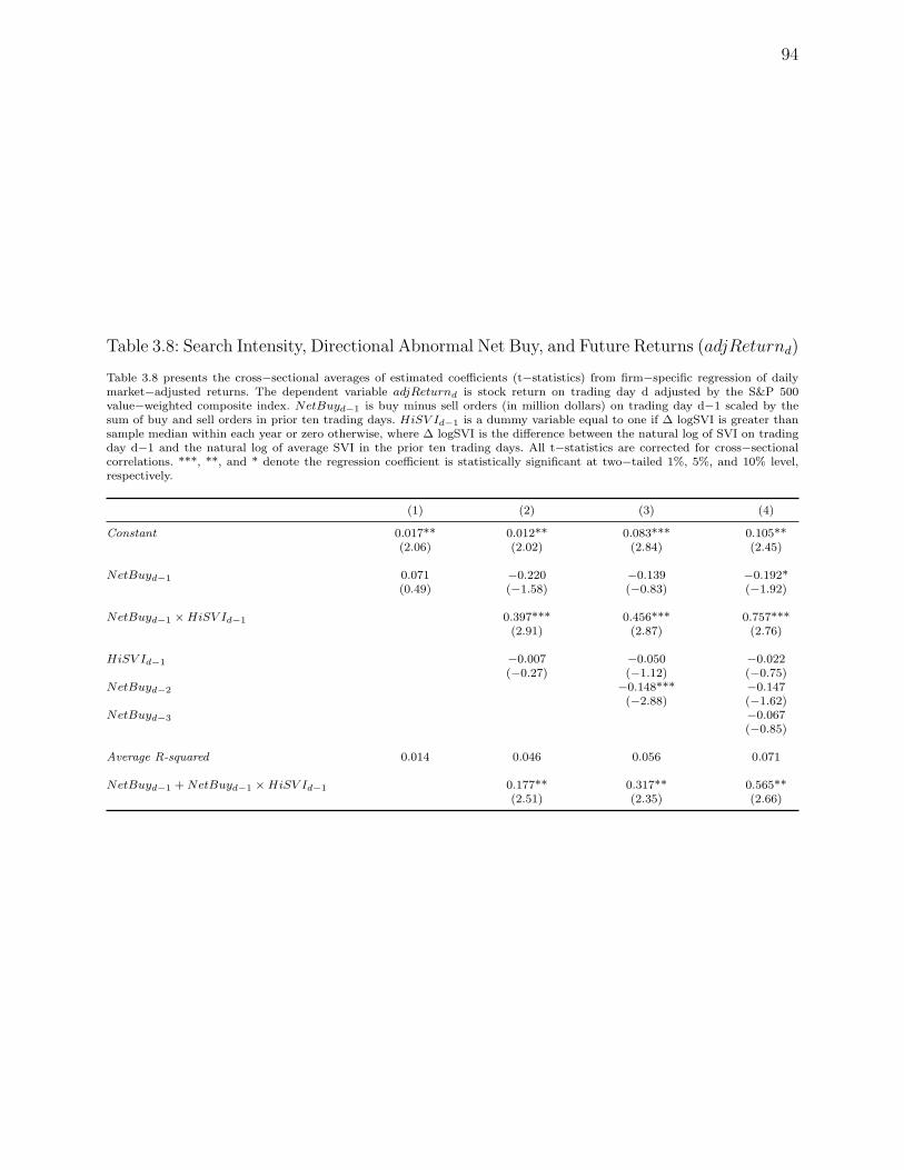
94

Table 3.8: Search Intensity, Directional Abnormal Net Buy, and Future Returns (adjReturnd)

Table 3.8 presents the cross−sectional averages of estimated coefficients (t−statistics) from firm−specific regression of dailymarket−adjusted returns. The dependent variable adjReturnd is stock return on trading day d adjusted by the S&P 500value−weighted composite index. NetBuyd−1 is buy minus sell orders (in million dollars) on trading day d−1 scaled by thesum of buy and sell orders in prior ten trading days. HiSV Id−1 is a dummy variable equal to one if ∆ logSVI is greater thansample median within each year or zero otherwise, where ∆ logSVI is the difference between the natural log of SVI on tradingday d−1 and the natural log of average SVI in the prior ten trading days. All t−statistics are corrected for cross−sectionalcorrelations. ***, **, and * denote the regression coefficient is statistically significant at two−tailed 1%, 5%, and 10% level,respectively.

(1) (2) (3) (4)

Constant 0.017** 0.012** 0.083*** 0.105**(2.06) (2.02) (2.84) (2.45)

NetBuyd−1 0.071 −0.220 −0.139 −0.192*(0.49) (−1.58) (−0.83) (−1.92)

NetBuyd−1 ×HiSV Id−1 0.397*** 0.456*** 0.757***(2.91) (2.87) (2.76)

HiSV Id−1 −0.007 −0.050 −0.022(−0.27) (−1.12) (−0.75)

NetBuyd−2 −0.148*** −0.147(−2.88) (−1.62)

NetBuyd−3 −0.067(−0.85)

Average R-squared 0.014 0.046 0.056 0.071

NetBuyd−1 +NetBuyd−1 ×HiSV Id−1 0.177** 0.317** 0.565**(2.51) (2.35) (2.66)