Electronic copy available at: http://ssrn.com/abstract=2356144

Dynamic Information Asymmetry, Financing,

and Investment Decisions∗

Ilya A. Strebulaev† Haoxiang Zhu‡ Pavel Zryumov§

January 26, 2014

Abstract

We reexamine the classic yet static information asymmetry model of Myers and Majluf

(1984) in a fully dynamic market. A firm has access to an investment project and can

finance it by debt or equity. The market learns the quality of the firm over time by

observing cash flows generated by the firm’s assets in place. In the dynamic equilibrium,

the firm optimally delays investment, but investment eventually takes place. In a

“two-threshold” equilibrium, a high-quality firm invests only if the market’s belief goes

above an optimal upper threshold, while a low-quality firm invests if the market’s belief

goes above the upper threshold or below a lower threshold. However, a different “four-

threshold” equilibrium can emerge if cash flows are sufficiently volatile. Relatively risky

growth options are optimally financed with equity, whereas relatively safe projects are

financed with debt, in line with stylized facts.

JEL Codes: G31, G32

Keywords: dynamic information asymmetry, investment, financing, pecking order

∗First version: June 2009. For helpful discussions and comments, we thank Anat Admati, Hui Chen,

Brett Green, Mike Harrison, Zhiguo He, Deborah Lucas, Leonid Kogan, Andrey Malenko, Erwan Morellec,

Stewart Myers, Jonathan Parker, Stephen Ross, Norman Schurhoff, Bilge Yilmaz, and seminar participants

at Stanford GSB, MIT, UNC-Duke Corporate Finance Conference, Wharton, Rochester Simon, HKUST,

Beijing University, Tsinghua University, EPFL, and University of Lausanne. Paper URL: http://ssrn.

com/abstract=2356144.†Graduate School of Business, Stanford University and NBER. Email: istrebulaev@stanford.edu.‡MIT Sloan School of Management. Email: zhuh@mit.edu.§Graduate School of Business, Stanford University. Email: zryumov pavel@gsb.stanford.edu.

Electronic copy available at: http://ssrn.com/abstract=2356144

Dynamic Information Asymmetry, Financing, andInvestment Decisions

January 26, 2014

Abstract

We reexamine the classic yet static information asymmetry model of Myers and Majluf

(1984) in a fully dynamic market. A firm has access to an investment project and can

finance it by debt or equity. The market learns the quality of the firm over time by

observing cash flows generated by the firm’s assets in place. In the dynamic equilibrium,

the firm optimally delays investment, but investment eventually takes place. In a

“two-threshold” equilibrium, a high-quality firm invests only if the market’s belief goes

above an optimal upper threshold, while a low-quality firm invests if the market’s belief

goes above the upper threshold or below a lower threshold. However, a different “four-

threshold” equilibrium can emerge if cash flows are sufficiently volatile. Relatively risky

growth options are optimally financed with equity, whereas relatively safe projects are

financed with debt, in line with stylized facts.

Electronic copy available at: http://ssrn.com/abstract=2356144

1 Introduction

The classic paper by Myers and Majluf (1984) begins by stating the following problem:

“Consider a firm that has assets in place and also a valuable real investment opportunity.

However, it has to issue common shares to raise part or all of the cash required to undertake

the investment project. If it does not launch the project promptly, the opportunity will

evaporate.” A major finding of Myers and Majluf (1984) is that adverse selection can cause

a financial market breakdown because the market cannot ascertain the quality of a firm’s

assets in place and will only offer a price that a high-quality firm finds too low to accept.

This market breakdown occurs in Myers and Majluf (1984) largely because the firm’s

manager has a single opportunity to make the investment. In many practical applications,

however, investment opportunities do not “evaporate” if not undertaken immediately. A

firm usually has the option to delay investment and financing if the market conditions are

unfavorable. In this paper, we reexamine the static problem of Myers and Majluf (1984) in

a fully dynamic market, in which a firm can choose the timing of its project as well as the

security it issues—debt or equity. The firm’s quality, or “type,” is determined by the average

cash flow of its assets in place. The market observes cash flows generated by the firm’s assets

in place and learns over time about the quality of the firm. If the firm decides to invest and

issue equity or debt, the market prices the offered security based on information revealed by

past cash flows and the firm’s actions. By delaying investment and financing, a high-quality

firm faces the following trade-off. On the one hand, the market will eventually ascertain

the true high quality of the firm, which minimizes the underpricing of its security. On the

other hand, delay costs the firm the time value of the investment project. A low-quality

firm faces a similar trade-off: by delaying, it loses the time value of the positive net present

value (NPV) of the project but can potentially benefit from the overpricing of its security

by pooling with a high-quality firm.

We present three main results in this paper. First, we characterize a strategic dynamic

equilibrium of investment and financing in this market. Unlike in the static equilibrium

of Myers and Majluf (1984), in our dynamic equilibrium, investment always takes place

eventually, if not immediately, and the market does not break down. More specifically, as

long as the market belief is not extremely high or extremely low, there is an initial, potentially

protracted, period of inaction, when no investment or issuance takes place. If the market’s

belief about the firm’s quality becomes sufficiently optimistic, both types invest. This upper

belief threshold is effectively chosen by a high-quality firm. Intuitively, if the market assigns

a high enough expectation of the value of the firm’s assets in place, the underpricing of the

1

newly issued security is small, and the high-quality firm optimally invests immediately. A

low-quality firm “imitates” a high-quality firm and invests as well. If the market’s belief

becomes sufficiently pessimistic, however, only a low-quality firm invests, thus revealing its

type to the market. The lower belief threshold is effectively chosen by the low-quality firm

such that it is indifferent between continuing to wait and investing immediately. Interestingly,

a low-quality firm invests probabilistically, not deterministically, at the lower threshold; the

investment probability is optimally chosen by the low-quality firm such that conditional on

observing no investment at the lower threshold, the market belief “reflects” upward. Put

together, the “two-threshold” equilibrium is characterized by three regions of the market’s

belief: an upper pooling region, a middle inaction region, and a lower separation region. The

qualitative nature of this dynamic equilibrium holds for both debt and equity.

Our second main result is to analyze the firm’s choice between debt and equity, two

most commonly used securities. The most natural theoretical benchmark is the pecking

order theory, as put forward by Myers (1984). The pecking order theory posits that debt is

preferred over equity in the presence of asymmetric information because debt is less sensitive

than equity to private information.

We find that the pecking order can be reversed if the new project is sufficiently risky.

Intuitively, risky projects that resemble a “gamble”—that is, projects with a small probability

of success but a large return conditional on success—are more likely to default if financed

with debt. In default, the original shareholders incur losses on assets in place that implicitly

serve as debt collateral. As the failure probability of the project increases, a high-quality firm

finds it particularly costly to issue debt. Therefore, high-risk projects tend to be financed

with equity, despite its dilutive nature. For relatively safe projects, debt is preferred to

equity. Importantly, this result comes from information asymmetry alone and does not rely

on deadweight costs of bankruptcy (which will make issuing debt even costlier) or any other

debt-related frictions. Our results can help explain a stylized fact that high-growth risky

projects (e.g., those financed by venture capital) tend to be financed by equity-like securities.

The combination of time-varying information asymmetry and security choice gives rise

to a new type of “four-threshold” equilibrium, if the volatilities of cash flows are sufficiently

high. The characterization of this four-threshold equilibrium is the third main result of our

study. This equilibrium features five regions of the market’s belief: two pooling regions (in

which both types of firms invest), two inaction regions (in which both types of firms wait

to invest), and one separation region (in which only the low-quality firm invests). Although

one of the inaction regions is similar to the inaction region in the two-threshold equilibrium,

2

the other inaction region occurs for an entirely different reason. Because a high-quality firm

can choose to finance a project with debt or equity, its static value function has a non-

differentiable point, a kink. At this kink, the high-quality firm will never invest; it would

rather delay and get a convex combination of its continuation values for issuing debt or

equity. Therefore, a new inaction region emerges around this kink. On either side of this

new inaction region are the two pooling regions, which have different securities in equilibrium.

We would like to emphasize that the four-threshold equilibrium distinguishes our analy-

sis from that of Daley and Green (2012), who extend the classical lemon’s problem of Akerlof

(1970) to a fully dynamic setting and derive a two-threshold equilibrium. In their model, a

seller wishes to sell an indivisible asset with unobservable quality, and buyers observe sig-

nals of the asset’s quality over time. Their model is essentially equity-only. Relative to the

results of Daley and Green (2012), we enrich the financing options of firms and characterize

the dynamic trade-off between debt and equity. As a result, the four-threshold equilibrium

emerges, and it is qualitatively different from the equilibrium of Daley and Green (2012).

Our results give rise to a number of empirical predictions. For example, security is-

suance is more likely when information asymmetry is less severe. This prediction is consistent

with Korajczyk, Lucas, and McDonald (1991), who find that “equity issues cluster in the

first half of the period between information releases . . . firms almost never issue equity just

prior to an earnings release.” Using analyst coverage as a proxy for information asymmetry,

Chang, Dasgupta, and Hilary (2006) find that firms covered by fewer analysts issue equity

less frequently.

A subtler but unique prediction of our model is that investment and issuance of debt

or equity can happen after a series of negative news. After sufficient price declines, a low-

quality firm has little chance of being mistaken for a high-quality firm; immediate issuance

thus becomes optimal. This prediction is consistent with stylized facts about stock price

behavior prior to equity issuance. For example, Korajczyk, Lucas, and McDonald (1990)

find that while most equity issuances take place after large positive abnormal returns, 18% of

issuances occur after share price declines relative to the market. A closely related empirical

prediction is that if issuance follows a series of negative news, post-issue price declines further

because issuance in this case is an additional signal of low firm quality.

Our results also predict that relatively safe projects are financed by debt, and rela-

tively risky projects are financed by equity. Frank and Goyal (2003) document that small,

high-growth firms tend to use equity financing instead of debt financing. This fact is often

interpreted as evidence against the pecking order theory, or as evidence that information

3

asymmetry is unimportant for capital structure decisions. Our results, however, reveal that

asymmetric information is perfectly consistent with, and may potentially explain, the pre-

dominant use of equity financing by small firms.

Our paper is related to several strands of the literature. Lucas and McDonald (1990)

also model dynamic information asymmetry by considering its impact on equity financing

decisions. In their model, information asymmetry is reset at fixed time intervals, so under-

valued firms do not issue equity until complete resolution of information asymmetry. The

immediate issuance by overvalued firms and the delayed issuance by undervalued firms jointly

predict an increase in share prices prior to issuance. In our model, by contrast, information

asymmetry is never completely resolved due to unpredictable shocks to cash flows. Thus,

a high-quality firm may still issue in the presence of underpricing, while a low-quality firm

may issue after a series of negative cash flow news.

Hennessy, Livdan, and Miranda (2010) develop a dynamic signaling model of invest-

ment and financing. In their paper, the firm’s manager has superior information relative

to the market, but this informational advantage is short lived. Markovian evolution of the

firm’s type together with short lived private information generate a time-invariant level of

information asymmetry in their model. In contrast, our model features time-varying infor-

mation asymmetry, stemming from persistent firm types and gradual information revelation.

In our dynamic equilibrium, the ability of the market to obtain a more precise estimate of

the firm’s type over time is the driving force behind the firm’s incentive to delay investment.

Investment delay in our model has an economic underpinning that is distinct from

those in the real option literature, where investment delays are caused by the optimal timing

of real option exercise. In a recent paper, Morellec and Schurhoff (2011) extend the Myers

and Majluf (1984) model to a real option setting, in which the firm chooses the optimal

investment timing, as well as the type of security to issue. They model the firm’s revenue

from the new project as the firm’s unobservable type multiplied by a publicly observable cash

flow process. The observable cash flow shocks in their model are independent of firm type and

hence cannot reveal information of the firm’s type over time. In our model, the market learns

about the firm’s type by observing its cash flows; the firm delays investment because learning

reduces adverse selection. In addition, Morellec and Schurhoff (2011) model the impact of a

positive deadweight cost of bankruptcy on the properties of a separating equilibrium, while

we concentrate on the information asymmetry mechanism alone.

We are not the first to propose a model in which the pecking order is partially reversed.

Fulghieri and Lukin (2001) show that debt might no longer be the preferred security if

4

investors endogenously acquire additional information about the issuer. Our results are

driven by a different channel, namely the trade-off between underpricing due to asymmetric

information and the risk of losing assets in place. A recent study by Fulghieri, Garcia, and

Hackbarth (2013) shows that equity can dominate debt if both the asset in place and the

growth option are subject to the type of asymmetric information that is similar to what we

examine here. Pecking order fails because the probability distribution of the firm’s value does

not satisfy the “conditional stochastic dominance,” under which debt is the optimal security

(Nachman and Noe (1994)). Fulghieri, Garcia, and Hackbarth (2013) investigate the optimal

security design problem under more general distributions of firm values, although information

asymmetry in their model is not time-varying. In contrast, we focus on the choice between

debt and equity and study time-varying asymmetric information and associated delays in

investment.

Chakraborty and Yilmaz (2011) show that in some situations the adverse selection

problem can be costlessly solved by the issuance of properly structured convertible debt.

Their result requires that (1) information asymmetry should be sufficiently low at the time

of maturity of the convertible debt, and (2) managers cannot benefit from the assets in place

or the growth option before the debt matures. In our setup, the availability of cash flows

prior to the resolution of market uncertainty limits the benefits of using convertible bonds.

In this respect, our results complement those of Chakraborty and Yilmaz (2011).

The rest of the paper is organized as follows. In Section 2, we present the static

model and equilibrium. In Section 3, we develop the dynamic model and study the dynamic

equilibria. In Section 4, we explore the welfare and empirical implications of our results. We

conclude in Section 5. All the proofs are in the Appendix.

2 Model Setup and Static Equilibrium

In this section, we develop and solve a static model of investment and financing decisions un-

der asymmetric information. Closely related to that of Myers and Majluf (1984), our static

model is simple yet sufficient to illustrate the intuition behind the main economic mecha-

nisms. For this reason, we keep as many standard assumptions of Myers and Majluf (1984)

as possible. In Section 3, we consider a fully dynamic model with asymmetric information

and compare its implications with this static benchmark. A glossary of key model variables

is also tabulated in the Appendix.

5

2.1 Model Setup

We start by introducing the economic agents, their strategy sets, and the model timeline.

2.1.1 The Firm and the Market

Consider an all-equity firm with pledgable assets in place that belong to one of two types

θ, θ ∈ H,L. The type is the private information of the firm’s management, which we

simply refer to as the “firm.” As in Myers and Majluf (1984), the existing shareholders are

passive, and there is no conflict of interest between existing shareholders and management.

All parameters other than the firm’s type are common knowledge. The firm’s assets in place

produce in expectation free cash flow µθ per unit of time, where µH > µL ≥ 0. Thus, the

firm is of high (low) quality if it is of the high (low) type. The cumulative cash flows of the

type θ firm at time t, Xθt , follow:

dXθt = µθdt+ σdBt, (1)

where µθ and σ are constants, and B = (Bt,FBt )t≥0 is a standard Brownian motion adapted

to the natural filtration defined on a canonical probability space (Ω, F , Q). The firm’s type

θ and the Brownian motion B are independent.

In addition to its assets in place, the firm has a risky growth option, which consists of a

monopoly access to a new production technology. At the time of investment, the firm pays a

one-time cost of I and installs the new technology. If the new technology succeeds, then the

expected free cash flow increases from µθ to µθ + K, where K is a positive constant that is

independent of θ. If, however, the new technology fails, the expected free cash flow remains

µθ. The success and failure of the new technology occur with respective probabilities γ and

1 − γ, independently of type θ and Brownian motion B. A type-independent new project

provides a clear benchmark and allows us to focus on the asymmetric information of assets

in place.1,2 The constant risk-free rate is r > 0. The NPV of the new project is thus kr− I,

where k ≡ γK. We assume that the NPV of the risky investment opportunity is positive:

1One could overlay asymmetric information about the new project by adjusting our model, but such anextension does not change our main results. For example, we can incorporate type-dependent K as follows.Denote the type-θ firm’s additional cash flow by Kθ, conditional on success. As long as µH +KH > µL+KL,and γ is common knowledge, we can show that the same solution procedure carries through and the qualitativenature of the equilibrium does not change.

2Heider (2005) considers a static setting in which a firm chooses one project among many that differ intheir risks and returns. His model does not have assets in place (that can be seized by debt holders) anddoes not consider dynamics.

6

k > Ir.

To make the firm’s problem non-trivial, we assume that the cost I must be entirely

financed by outside investors. Alternatively, we can interpret the cost I as the net funds that

the firm must raise above and beyond its internal resources. In addition, the firm is unable to

spin-off the growth option and finance it independently of the assets in place. These realistic

assumptions on the firm are consistent with those of Myers and Majluf (1984).

Given that the mean cash flow of the firm is at least µL, any funding decision will involve

the firm optimally pledging the assets in place and raising secured, risk-free debt with a face

value of µL/r. The amount µL/r then effectively represents the financial resources available

to the firm; regardless of adverse selection, it reduces the required funds I that must be raised

from outside investors. We therefore can assume that µL = 0. In other words, the mean cash

flow µθ and the required investment I should be interpreted as those after the firm exhausts

its capacity of issuing secured, risk-free debt. Any other debt issued afterwards is junior to

the secured debt. For simplicity, we refer to the junior debt simply as “debt,” bearing in

mind that there could be senior debt, which is secured and risk-free but is irrelevant for our

analysis of adverse selection.

There is a group of competitive outside investors, called the “market,” that does not

observe θ. The market has a prior belief p0 ∈ [0, 1] at time 0 that the firm is of type H, and

1 − p0 that the firm is of type L. The market and the firm are risk-neutral. There are no

taxes or deadweight default costs in our model.

2.1.2 Timeline and Strategies

We now formally describe the timing of the static model and the strategies of the firm and

the market.

1. The firm observes θ; the market does not.

2. The market quotes prices of debt and equity for the firm in anticipation of investment.3

In return for providing the funds I, the market demands a fraction λ of the firm’s total

equity or a perpetual debt with coupon payment c.

3. Upon observing the quotes λ and c, the firm decides whether to invest or not and

which security to use conditional on investment. The firm’s strategy is a probability

distribution over the set of feasible actions a ∈ A = ∅, e, d, conditional on quoted

3We restrict attention to debt and equity because they are the most commonly used securities in practice.The problem of optimal security design, albeit interesting, is not the objective of this study.

7

λ and c, where a = ∅ denotes no investment, a = e denotes investment with equity

financing, and a = d denotes investment with debt financing.

A type θ firm chooses the probabilities of equity offering, πe(θ), debt offering, πd(θ),

and no investment, 1−πe(θ)−πd(θ).4 For simplicity, a firm can finance the project by

issuing equity only or debt only, but not a combination of the two.5 If the firm decides

not to invest at time 0, the game is over.

4. If the investment takes place, it is immediately revealed to be successful or unsuccessful.

Since the firm’s post-investment mean cash flow and coupon obligation (if debt is

issued) are both constants, the firm defaults immediately if and only if the mean cash

flow is lower than the coupon level.6 If default occurs, the investors seize the firm’s

assets without incurring any deadweight cost, and the game ends.

We can write down the payoffs of the players as follows. The expected payoff E to the

firm for passing on the investment opportunity, investing with equity financing, or investing

with debt financing are, respectively,

E∅θ =µθr, (2)

Eeθ(λ) = (1− λ)

µθ + k

r, (3)

Edθ (c) = γmax

(µθ +K − c

r, 0

)+ (1− γ) max

(µθ − cr

, 0

). (4)

The max( · ) operator in Edθ (c) reflects the fact that the firm defaults if the post-investment

mean cash flow is lower than the debt coupon.

4Probabilities of investment with a particular kind of financing depend on the observed market quotes λand c, i.e., πe(θ) = πe(θ;λ, c) and πd(θ) = πd(θ;λ, c). For brevity, we suppress the function arguments (λ, c)of πe and πd.

5This assumption is without loss of generality in our setup. Allowing the market to quote prices forpartial financing expands the space of deviations, but our equilibrium still survives.

6Strictly speaking, because the cash flows are risky, there is positive probability that the high type firm’scumulative cash flow in the small interval (t, t + dt) falls below cdt, even if the project is successful. Todeal with this technicality, we assume that the firm can access instantaneous (overnight) credit for thistype of cash shortfalls. Importantly, this instantaneous credit is small in magnitude and cannot satisfy theinvestment need I.

8

Similarly, the expected payoff S to the market facing a type θ firm in cases of a = e

and a = d are, respectively,

Seθ(λ) = λµθ + k

r− I, (5)

Sdθ (c) = γmin

(c

r,µθ +K

r

)+ (1− γ) min

(cr,µθr

)− I. (6)

Because the market does not observe θ, it has to infer the average quality of the firm

attracted by the offer (λ, c), according to Bayes’ rule. The probability of the firm being the

high type, conditional on investment with debt (or equity) financing, is equal to:

qi0 =p0π

i(H)

p0πi(H) + (1− p0)πi(L), if πi(H) + πi(L) > 0, for i = e, d. (7)

In particular, if the firm uses deterministic strategies, (7) simplifies to:

qi0 =

p0, if πi∗(H) = 1 and πi∗(L) = 1,

1, if πi∗(H) = 1 and πi∗(L) = 0,

0, if πi∗(H) = 0 and πi∗(L) = 1.

for i ∈ e, d. (8)

In other words, given λ and c, if a specific security (debt or equity) is selected by one type

of firm but not the other, the market immediately and correctly separates the two types. If

both types invest using the same security, the market keeps its prior.

The expected payoffs to the market, Se(λ) and Sd(c), are then given by:

Se(λ) =

qe0SeH(λ) + (1− qe0)SeL(λ), if πe(H) + πe(L) > 0

0, if πe(H) + πe(L) = 0,(9)

Sd(c) =

qd0SdH(c) + (1− qd0)SdL(c), if πd(H) + πd(L) > 0

0, if πd(H) + πd(L) = 0.(10)

Given the strategies and payoffs, a perfect Bayesian equilibrium of the static game

consists of the strategy (πd∗(θ), πe∗(θ)) of the firm and quotes (c∗, λ∗) of the market such

that: (i) the firm maximizes its payoff; (ii) the market breaks even in expectation, and the

corresponding qi0 is consistent with πi∗ in the sense of (7); and (iii) there does not exist

another pair of quotes (λ, c) that earns strictly positive profits for the market given πe∗ and

9

πd∗.7

Without loss of generality, we impose the following tie-breaking rules in the static

model. First, if the firm is indifferent between investing and not investing, the firm invests.

Second, if the firm is indifferent between issuing debt or equity, the firm issues equity.

Finally, if the market is indifferent between buying the firm’s equity or debt and not buying

it, the market buys it. Under the tie-breaking rules, it often suffices to write the parameter

conditions using strict inequalities in our equilibrium characterization.

2.2 Economic Forces

In this section, we discuss the key trade-offs and economic mechanisms of the static game,

which are also relevant for the dynamic model. The three possible actions of the firm,

A = ∅, e, d, give rise to three different pairwise trade-offs: investment with equity financing

versus no investment, investment with debt financing versus no investment, and investment

with debt versus investment with equity. We start by analyzing these trade-offs one by

one because it simplifies the expositions of our results later. For example, we find that the

conventional pecking order can be reversed even in such a simplistic static environment, that

is, equity financing can dominate debt financing under asymmetric information.

2.2.1 Investment with Equity Financing vs. No Investment

Upon equity offering, to break even on its investment, the competitive market would have

to demand a fraction λ of the firm that satisfies:

I = λ

(qe0µH + k

r+ (1− qe0)

µL + k

r

). (11)

The right-hand side of (11) is the value of outside investors’ equity. The value of λ is then:

λ(qe0) =Ir

qe0(µH + k) + (1− qe0)(µL + k). (12)

A low type firm strictly prefers investing. Intuitively, its worst-case scenario is to

invest in the positive-NPV project while revealing its type, and the best-case scenario is to

7Condition (iii) is a slight generalization of the “No Unrealized Deals” condition of Daley and Green(2012). Conditions (ii) and (iii) ensure that market offers are competitive.

10

be mistaken for a high type firm. Thus, for any belief qe0,

EeL(λ) > E∅L. (13)

For a high type firm, equity issuance involves a trade-off between the benefits of the

positive-NPV project and the costs of subsidizing a low type firm. A high type firm strictly

prefers equity financing (thus pooling with the low type) if and only if:

EeH(λ) > E∅H . (14)

By (12), (14) holds if and only if:

qe0 ≥ pe ≡Ir

k

µH + k

µH − µL− µL + k

µH − µL. (15)

It is easy to check that pe < 1. The level of pe thus establishes a belief threshold, with a

high type firm always issuing equity if the market beliefs are sufficiently high.

Lemma 1. For all market beliefs, a low type firm prefers investment with equity financing

to no investment. A high type firm prefers investment with equity financing to no investment

if and only if qe0 ≥ pe.

Lemma 1 restates a celebrated result of Myers and Majluf (1984) that, in the mold of

Akerlof (1970), asymmetric information can prevent the market from providing financing for

positive NPV projects. The economic thrust of the mechanism is that a decision to invest

and issue equity can be interpreted by the market as a signal of the low quality of a firm’s

assets, which is immediately reflected in the share price. Low equity prices, in turn, deter a

high type firm from investing in the first place.

2.2.2 Investment with Debt Financing vs. No Investment

We now turn to the comparison between investment with debt financing and no investment.

Clearly, neither type defaults if the project is successful.8 However, a low type firm always

defaults if the project fails. Therefore, two scenarios can arise in the case of project failure:

(i) only a low type firm defaults; and (ii) both types default. We consider both cases in turn.

8To see this, consider the debt coupon of Ir/γ. The market breaks even because its payoff is at leastγ × Ir/(rγ) = I. Because k > Ir, Ir/γ < k/γ = K, and no firm defaults upon project success.

11

Case 1. Suppose that only the low type defaults if the project fails. To break even the

market has to demand a perpetuity with coupon c that satisfies:

I = qd0c

r+ (1− qd0)γ

c

r, (16)

or c(qd0) =Ir

1− (1− qd0)(1− γ). (17)

A high type firm does not default if and only if µH ≥ c(qd0), or

qd0 ≥ pr ≡ 1− 1

1− γ

(1− Ir

µH

). (18)

Thus, pr is the belief threshold above which a high type firm does not default in this case.

Case 2. Suppose that both types of firms default if the project fails. To break even the

market demands a perpetuity with coupon c that satisfies:

I = γc

r+ (1− γ)qd0

µHr, (19)

or c(qd0) =Ir − (1− γ)qd0µH

γ. (20)

It is easy to show that the incentive condition for a high type firm to default is qd0 < pr.

Combining (17) and (20), the break-even coupon level is:

c(qd0) =

Ir1−(1−qd0)(1−γ)

, if qd0 > pr,

Ir−(1−γ)qd0µHγ

, if qd0 ≤ pr.(21)

A low type firm always prefers investing with debt issuance to no investment. Upon

project failure, it defaults and loses nothing, whereas project success brings not only the

positive value of the project but also the benefits from a lower coupon due to overpriced

debt. Formally,

EdL(c(qd0)) = γ

K − c(qd0)

r> E∅L = 0, ∀ qd0 ∈ [0, 1]. (22)

For a high type firm, debt issuance involves a trade-off between the benefits of the

positive project NPV and the costs of subsidizing a low type firm. A high type firm strictly

prefers debt financing (thus pooling with the low type) if and only if:

EdH(c(qd0)) ≥ E∅H . (23)

12

By equations (2), (4), and (21), condition (23) holds if and only if:

qd0 ≥ pd =

1− k−Irk(1−γ)

, if µH ≥ k;

1− k−IrµH(1−γ)

, if µH < k.(24)

The level of pd thus establishes a belief threshold, with a high type firm always issuing

debt (rather than not investing) if the market belief is sufficiently high.

Lemma 2. For all market beliefs, a low type firm prefers investment with debt financing to

no investment. A high type firm prefers investment with debt financing to no investment if

and only if qd0 ≥ pd.

Lemma 2 is similar to Lemma 1. In both cases, a low type firm always prefers investing,

and a high type firm prefers investing only if the corresponding market belief is sufficiently

high. This similarity stems from the absence of taxes and default costs in our model.

2.2.3 Equity Financing vs. Debt Financing

We now explore the decision to issue debt or equity. We focus on a high type firm because it

determines the type of security issued in the equilibrium. Using (3) and (12), we can write

the high type firm’s value in the equity issuance case, EeH , as:

EeH((λ(qe0)) =

(1− λ(qe0)

)µH + k

r

=µHr︸︷︷︸

PV assets in place

+

(k

r− I)

︸ ︷︷ ︸NPV of the project

− I(1− qe0)µHqe0µH + k︸ ︷︷ ︸

Loss due to underpricing

. (25)

Similarly, using (4) and (21) we write the high type firm’s value in the debt issuance

case as:

EdH(c(qd0)) = γmax

(µH +K − c(qd0)

r, 0

)+ (1− γ) max

(µH − c(qd0)

r, 0

)=

µHr︸︷︷︸

PV assets in place

+

(k

r− I)

︸ ︷︷ ︸NPV of the project

− (1− γ)(1− qd0) min

(µHr,

I

1− (1− γ)(1− qd0)

)︸ ︷︷ ︸

Loss due to underpricing and default

,

(26)

where the min(·) operator reflects the fact that a high type firm may or may not default.

13

Hence, the comparison of EdH and Ee

H boils down to the comparison between losses from

underpricing.

Note that, under debt financing, a high type firm’s loss due to underpricing depends

on the probability of success γ, but not on the expected payoff k. Under equity financing,

the reverse is true. Intuitively, debt holders do not benefit from the upside of the project and

are only concerned as to whether or not the coupon is paid in full. New equity holders, by

contrast, face no default risk and only care about the NPV of the project. The comparison

between EdH and Ee

H therefore eventually depends on the interplay between the success

probability and the project NPV.

Lemma 3 below compares EdH and Ee

H under an additional conjecture, later verified

in equilibrium, that the type of financing does not affect market beliefs, that is, qe0 = qd0 =

q0 = p0. This comparison proves particularly useful for characterizing the equilibrium in

Proposition 1.

Lemma 3. Define pd/e as:

pd/e =1

µH

(Ir

1− γ− k). (27)

1. A high type firm prefers debt to equity if and only if either of the two following condi-

tions holds:

(a) q0 < pr and q0 < pd/e,

(b) q0 > pr and γ > kk+µH

.

2. A high type firm prefers equity to debt if and only if either of the two following condi-

tions holds:

(a) q0 < pr and q0 > pd/e,

(b) q0 > pr and γ < kk+µH

.

Figure 1 shows a typical debt-versus-equity choice of a high type firm in the (γ, p0)

space, keeping the NPV of the project k/r− I fixed. We can see that for a fixed p0, a higher

γ favors debt, whereas a lower γ favors equity. On the one hand, if the probability of success,

γ, is low, the project is effectively a “gamble:” it is unlikely to succeed, but conditional on

success, its return K is large. In this case, debt financing leads to a high probability of

default, whereas equity financing assures that the firm keeps its assets in place. Even if the

high type firm never defaults on its debt, debt is still inferior to equity because debt holders

14

Figure 1: Debt vs. Equity Regions

Equity Debt

p

0 kµH+k

10

1

p d/e

p r

Student Version of MATLAB

do not participate in the upside K. Equity therefore dominates debt for low values of γ.

On the other hand, if γ is large, default and the subsequent loss of assets in place is less

likely. Debt then allows a high type firm to lower its financing cost associated with adverse

selection. Naturally, as the initial market belief increases, equity becomes less costly because

of the lower adverse selection impact. We further illustrate the properties of this trade-off

in Section 2.3, where we present the static equilibrium.

2.3 Static Equilibrium

Having analyzed the pairwise trade-offs, we are now ready to state the equilibrium. Propo-

sition 1 characterizes the perfect Bayesian equilibrium of the static model.

Proposition 1. (Static Perfect Bayesian Equilibrium) There exists a unique perfect

Bayesian equilibrium with the following strategies:

1. Debt pooling:

(a) If p0 < pr, p0 < pd/e, and p0 > pd, then both types of firms issue debt with coupon

c∗ = Ir−(1−γ)p0µHγ

. If the project fails, both types default.

(b) If p0 > pr, γ >k

k+µH, and p0 > pd, then both types of firms issue debt with coupon

c∗ = Ir1−(1−p0)(1−γ)

. If the project fails, only a low type firm defaults.

2. Equity pooling: If either of the following two conditions is satisfied, both types of firms

issue equity with λ∗ = Irp0µH+k

:

15

(a) p0 < pr, p0 > pd/e, and p0 > pe;

(b) p0 > pr, γ <k

k+µH, and p0 > pe.

3. Separation: If p0 < min(pe, pe), only a low type firm invests by issuing equity with

λ∗ = Irk

.

In all cases, if the firm issues a security that is off-equilibrium, the market belief is that such

deviation is done by a low type firm.

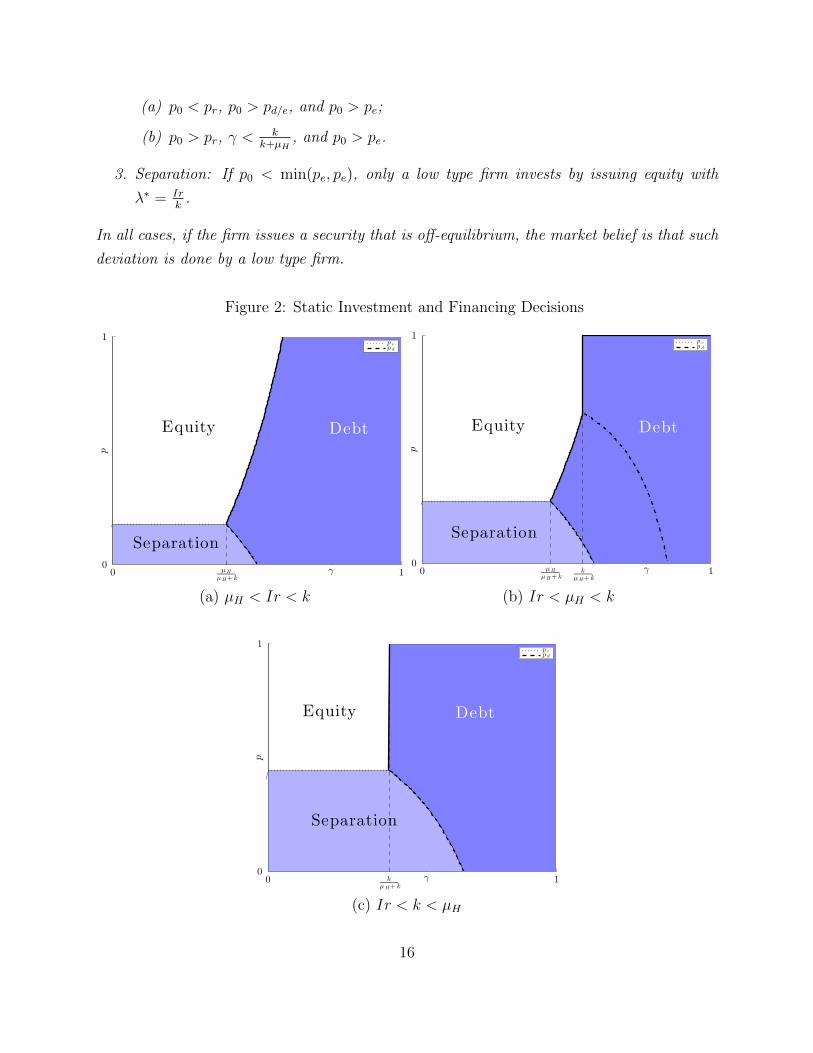
Figure 2: Static Investment and Financing Decisions

Equity Debt

Separation

p

0 µH

µH+ kγ 1

0

1p ep d

Equity Debt

Separation

p

0 µH

µH+ kk

µH+ kγ 1

0

1p ep d

(a) µH < Ir < k (b) Ir < µH < k

Equity Debt

Separation

p

0 kµH+ k

γ 10

1p ep d

(c) Ir < k < µH

16

Figure 2 illustrates the equilibrium strategies of Proposition 1 in the (γ, p0) space,

keeping the NPV of the project k/r − I fixed. There are three cases, depending on the

expected cash flow of a high type’s assets in place, µH . In all cases, a high type firm

prefers not to invest when both the market belief and new project’s success probability are

low. Equity is preferred when the market belief is sufficiently high but the project fails

with a high probability. Debt is preferred if the project succeeds with a high probability.

Graphically, part (b) of Figure 2 is obtained by “carving out” a separation region—a low

belief p0 and a low success probability γ—out of Figure 1. We emphasize that the high type

firm is never able to separate itself from the low type in equilibrium. Intuitively, because

there is no deadweight cost of default, the low type firm will always imitate the high type

firm. There is no credible “signaling” that the high type can use to prevent the low type

from imitating.

In addition to confirming the intuition of Myers and Majluf (1984) that adverse se-

lection can prevent positive NPV investments, Proposition 1 also has a salient feature: the

partial violation of the pecking order theory of Myers (1984). We demonstrate that even in a

simple economic environment like ours, debt is not necessarily better than equity. Nachman

and Noe (1994) characterize a sufficient condition, called “conditional stochastic dominance,”

under which debt is the optimal security design under asymmetric information. This condi-

tion is violated in our model.

Proposition 1 also informs the debt-versus-equity choices of firms with a large asset in

place or a large growth option. For example, in Part 1(b) of Proposition 1, the condition

γ > k/(k + µH) can be rewritten as µH > k(1 − γ)/γ. That is, for fixed γ, if the asset in

place, µH , is large relative to the expected project value k, then debt is preferred; otherwise

equity is preferred.

3 Dynamic Investment and Financing

In this section, we extend the static framework of Section 2 to a fully fledged dynamic

environment. The dynamic market introduces two critical changes. First, the firm’s manager

can flexibly decide the timing of investment: the investment option does not “evaporate” if

not taken at date 0. Second, the market learns the true quality of the firm over time even

in the absence of investment announcements. In postponing the investment, a high type

firm therefore weighs the cost of losing cash flows by not exercising the profitable growth

option immediately and the benefit of gaining from the market’s upward belief update over

17

time. A low type firm, by contrast, faces the trade-off between investing immediately, which

instantaneously increases its cash flows at the cost of revealing its type, and waiting for a

high type firm to invest, which gives it an opportunity to pool. These intricate dynamic

trade-offs significantly alter the equilibria of the model. A glossary of key model variables

used in this section is also tabulated in the Appendix for the ease of reference.

3.1 Timing of the Dynamic Model

The firm can decide to invest at any time t, t ≥ 0. The total amount of funds I required

for investment must be raised at the same time.9 The market’s belief that it is facing a high

(respectively, low) type firm at any time t, conditional on no investment up to time t, is

given by pt (respectively, 1 − pt), 0 ≤ pt ≤ 1. If the firm issues equity (debt) at time t, it

does so at the quoted price λt (ct). All players’ decisions at time t are conditioned on the

history of cash flows, market offers, and market beliefs available up to time t. Formally, the

history of these variables is adapted to the filtration Gt, generated by the family of random

variables Xs, ps, λs, cs; s ≤ t.We assume that the cash flows Xt from assets in place are paid out to the existing

shareholders immediately and cannot be accumulated inside the firm. If the firm were able

to accumulate cash over time, one would expect the high type firm to have a higher incentive

to delay investment, as cash accumulation reduces the required amount of external funds.

Therefore, abstracting away from this additional delay incentive is likely to understate the

effect of dynamic asymmetric information on investment and financing behavior.10

The timing of the dynamic game is as follows:

1. Nature draws the firm’s type θ ∈ H,L, according to the probability distribution

given by the prior (p0, 1 − p0), independently from B. The firm observes θ but the

market does not.

2. At every moment of time t, the market quotes the prices of debt and equity for the firm

in anticipation of immediate investment. In return for funds I, the market demands

a fraction λt of the firm’s total equity or a perpetual debt with coupon payment ct,

9The dynamic equilibrium survives if we allow for several stages of fund raising, because a high type firmfinds it optimal to raise the full amount in one stage and a low type firm would be forced to mimic.

10Although this assumption is restrictive, a dynamic problem with two state variables—market beliefand inside cash—is technically hard to solve explicitly. To illustrate the intuition, however, we providean explicitly solved two-period model with information asymmetry and cash accumulation in the OnlineAppendix of this paper.

18

conditional on the observed history Gt−.11 (Without cash accumulation, the required

investment I does not change over time.)

3. The firm’s action is defined by a pair of processes (πet (θ), πdt (θ)).

12 Define

πt(θ) = πdt (θ) + πet (θ) ≤ 1, ∀ t ≥ 0, (28)

where πt(θ) is the cumulative probability of issuance up to time t, with πdt (θ) and

πet (θ) being its debt and equity components. As an example, consider the following

“pure” strategy used by a high type firm: issue debt with probability 1 as soon as the

market’s belief pt hits an upper threshold p and never issue equity. The corresponding

(πd(H), πe(H)) is:

πdt (H) =

0, if sup

s≤tps < p

1, if sups≤t

ps ≥ pπet (H) ≡ 0. (29)

The general definition of strategies allows the firm to mix every instance between

issuing equity, issuing debt, and waiting with “probabilities”dπe

t (θ)

1−πt−(θ),

dπdt (θ)

1−πt−(θ), and

1 − dπet (θ)+dπd

t (θ)

1−πt−(θ), respectively.13 The firm may choose not to invest at all, that is,

P(

limt→∞

πt(θ) = 1)

could be less than 1.

4. If the investment takes place, it is immediately revealed to be successful or unsuccessful.

Since the firm’s post-investment mean cash flow and coupon obligation (if debt is

issued) are both constants, the firm defaults immediately if and only if the mean cash

flow is lower than the coupon level. If default occurs, the investors seize the firm’s

assets without incurring any deadweight loss and the game ends.

11As standard, Gt− = ∪s<tGs.12More rigorously, πd(θ) and πe(θ) are cadlag (right continuous with existing left limits) non-decreasing

processes adapted to (Gt)t≥0 that satisfy 0 ≤ πdt (θ) + πet (θ) ≤ 1 for all t ≥ 0. We allow for both flow andjumps in the firm’s distribution of investment decisions.

13As standard, πt−(θ) stands for the left limit lims↑t πs(θ). The formal definition of dπit(θ) for i ∈ d, eis omitted for brevity. We use this notation as a shorthand for two important scenarios: (i) if there is adiscrete jump in the probability of investment, then dπit(θ) = πit(θ) − πit−(θ); and (ii) if only a high (low)type firm invests with a positive probability, the ratio dπit(H)/dπit(L) equals to +∞ (0), in which case theexact meaning of dπit(L) (dπit(H)) is irrelevant.

19

If the firm invests at time t, the payoff to the firm’s existing shareholders is:

Eeθ(λt) = (1− λt)

µθ + k

r, (30)

Edθ (ct) = γmax

(µθ +K − ct

r, 0

)+ (1− γ) max

(µθ − ctr

, 0

), (31)

and the payoff to the market facing a type θ firm is given by:

Seθ(λt) = λtµθ + k

r− I. (32)

Sdθ (ct) = γmin

(ctr,µθ +K

r

)+ (1− γ) min

(ctr,µθr

)− I. (33)

Because the market does not observe θ, it has to infer the average quality of the firm attracted

by the offer λt (or ct), according to Bayes’ rule. The probability of the firm being of high

type conditional on investment with debt (or equity) financing is determined from:

qit1− qit

=p0

1− p0

· ϕHt (Xt)

ϕLt (Xt)· dπ

it(H)

dπit(L)when dπit(H) + dπit(L) > 0, (34)

where ϕθt (·) is the probability density function of the normal N (µθt, σ2t) random variable.

The expected payoffs to the market, Se(λt) and Sd(ct), are then given by:

Se(λt) = [qetSeH(λt) + (1− qet )SeL(λt)] · 1(dπet (H) + dπet (L) > 0), (35)

Sd(ct) = [qdt SdH(ct) + (1− qdt )SdL(ct)] · 1(dπdt (H) + dπdt (L) > 0). (36)

3.2 Equilibrium of the Dynamic Model

The nature of dynamic equilibrium depends on the primitive model parameters (µH , I, r, k, γ, σ)

and the structure of the corresponding static equilibrium. For simplicity of exposition, we

enumerate various parameter cases below. Each case represents a distinct economic scenario.

Definition 6 in the Appendix enumerates these cases in terms of the primitive parameters.

Definition 1. We define the parameter regions as follows.

Case I: Primitive model parameters satisfy one of the restrictions 1(a), 1(b′), 2(a),

2(b′), or 3(a) of Definition 6. These restrictions are generally satisfied for low and inter-

mediate values of the new project’s success probability γ, with the additional restriction that

volatility σ is small when γ takes intermediate values.

20

Case II: Primitive model parameters satisfy restriction 1(c) of Definition 6. This

condition is satisfied when the project is sufficiently safe but the debt of a high type firm is

risky regardless of market beliefs.

Case III: Primitive model parameters satisfy restriction 2(c′) or 3(b) of Definition 6.

These restrictions are generally satisfied when the project is sufficiently safe, σ is small, and

a high type firm never defaults on its debt when the market is sufficiently optimistic.

Case IV: Primitive model parameters satisfy restriction 1(b′′) or 2(b′′) of Definition

6. These conditions are generally satisfied for intermediate values of γ and high values of σ.

Case V: Primitive model parameters satisfy restriction 2(c′′) of Definition 6. These

restrictions are generally satisfied when the project is sufficiently safe, σ is large, and a high

type firm never defaults on its debt when the market is sufficiently optimistic.

Cases I–III give rise to a two-threshold dynamic equilibrium described in Proposition 2.

Cases IV and V give rise to a four-threshold dynamic equilibrium characterized in Proposition

4. We start by defining a perfect Bayesian equilibrium in the dynamic model.

Definition 2. A perfect Bayesian equilibrium of the dynamic model consists of a pair of

strategies (πd∗(θ), πe∗(θ)) of the firm and (λ∗, c∗) of the market, and the market belief p, such

that:

1. For each type θ, the strategy (πd∗(θ), πe∗(θ)) maximizes the value of the firm’s original

shareholders, given the market’s strategy (λ∗, c∗) and beliefs p:

(πd(θ), πe(θ)) ∈ arg max(πd,πe)

E

[∫ ∞0

(∫ t

0

e−rudXu

)d(πet + πdt )

+

∫ ∞0

e−rt(Eeθ(λt) dπ

et + Ed

θ (ct) dπdt

)]. (37)

2. Conditional on the firm’s investment at time t, the market earns zero profits:

Se(λt) = 0 Sd(ct) = 0, (38)

where the probabilities qet and qdt are consistent with πe∗(θ) and πd∗(θ) in the sense of

(34).

3. There does not exist another pair of quotes (λ, c) adapted to Gt− that earns strictly

positive profits for the market given πe∗(θ) and πd∗(θ).

21

4. The market belief p is consistent with (πd∗(θ), πe∗(θ)), i.e., it satisfies Bayes’ rule along

the equilibrium path:

pt1− pt

=p0

1− p0

· ϕHt (Xt)

ϕLt (Xt)·

1− π∗t−(H)

1− π∗t−(L), (39)

where ϕθt (·) is the probability density function of the normal N (µθt, σ2t) random vari-

able.

The firm’s value in (37) is decomposed into two components. The first component is

the present value of cash flows generated by assets in place that the firm receives until the

exercise of the growth option. The second component is the discounted value of the firm’s

(old) equity after new funds are raised and the growth option is exercised. The sum of these

two components is integrated over the equilibrium strategy (πe∗, πd∗) that determines the

timing of the investment and the type of security used.

To explore the evolution of the market’s belief, note that as long as no investment has

occurred, the market revises its belief based on two sources of information: publicly available

cash flows and equilibrium investment strategies. The former gives rise to the non-strategic

component of the belief process, while the latter gives rise to the strategic (signaling) one.

To disentangle these two components, as well as to simplify exposition, we introduce an

auxiliary belief process Pt, which is defined as:

Pt1− Pt

=p0

1− p0

· ϕHt (Xt)

ϕLt (Xt). (40)

The process Pt encapsulates the probability of facing a high type firm, conditional only

on the observed cash flows up to time t. In other words, Pt represents the non-strategic

component of the belief process.

To demonstrate the effect of the second, strategic, source of information, define zt

as zt = ln(

pt1−pt

)and the corresponding auxiliary process Zt as Zt = ln

(Pt

1−Pt

). Then,

equations (39) and (40) can be rewritten as:

zt = Zt + ln

(1− π∗t−(H)

1− π∗t−(L)

), (41)

Zt = ln

(p0

1− p0

)+µH − µL

σ2

(Xt −

µH + µL2

t

). (42)

The second term in (41) captures the pure signaling effect on the market’s belief. Obviously,

22

Zt = zt as long as there is no investment (i.e., if πt(H) = πt(L) = 0).

As Zt is monotone in Pt and zt is monotone in pt, we can also refer to Zt and zt as the

market’s “belief” processes. The market’s belief process Zt does not depend on the firm’s

type. The firm, however, knows its type, and the manager observes the “true” belief process

Zt, denoted Zθt . Substituting (1) into (42), we can write:

dZHt =

h2

2dt+ hdBt, (43)

dZLt = −h

2

2dt+ hdBt, (44)

where h = (µH − µL)/σ. Path by path, Zt coincides with ZHt if the firm is of the high type,

while it coincides with ZLt if the firm is of the low type. At any instance s, the market’s

conditional distribution of future realizations of Zt, t > s, is given by (42), the high type’s

corresponding distribution of ZHt is given by (43), and the low type’s conditional distribution

of ZLt is given by (44). This difference in the assessment of future conditional distributions

is the essential source of dynamic information asymmetry.

The advantage of using Zt is that it is the only state variable that affects decision-

making. Note that (42) establishes the linear relation between three potential state variables:

time t, cumulative cash flow Xt, and belief Zt. Cash flow Xt and time t affect strategies only

through their linear combination Xt− (µH + µL)t/2. Thus, the dependence of Zt on Xt and

t is implicit.

Following Daley and Green (2012), we introduce belief processes and a strategy profile

Ξi(z, z), where (z, z), z < z is a pair of threshold beliefs and i ∈ d, e denotes whether the

two types of firms pool at the upper threshold z with debt (superscript “d”) or with equity

(superscript “e”), whenever pooling occurs.

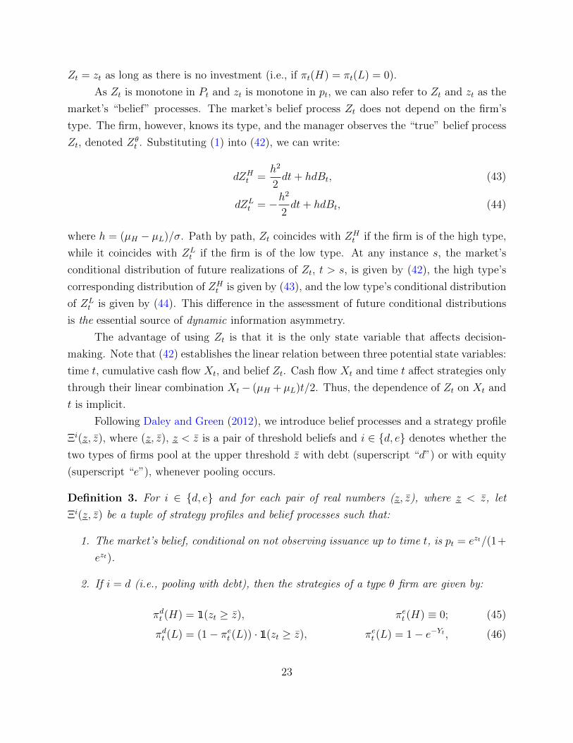
Definition 3. For i ∈ d, e and for each pair of real numbers (z, z), where z < z, let

Ξi(z, z) be a tuple of strategy profiles and belief processes such that:

1. The market’s belief, conditional on not observing issuance up to time t, is pt = ezt/(1+

ezt).

2. If i = d (i.e., pooling with debt), then the strategies of a type θ firm are given by:

πdt (H) = 1(zt ≥ z), πet (H) ≡ 0; (45)

πdt (L) = (1− πet (L)) · 1(zt ≥ z), πet (L) = 1− e−Yt , (46)

23

where 1(·) is the indicator function and

Yt = max

(z − inf

s≤tZs, 0

). (47)

3. If i = e (i.e., pooling with equity), then the strategies of a type θ firm are given by:

πet (H) = 1(zt ≥ z), πdt (H) ≡ 0; (48)

πet (L) =

1, if sup

s≤tzs ≥ z;

1− e−Yt , if sups≤t

zs < z;πdt (L) ≡ 0. (49)

4. The market offers at time t correspond to the beliefs:

qit = pt · 1(zt ≥ z), q−it ≡ 0, (50)

where notation “−i” refers to the security other than i.

In other words, this strategy is a “two-threshold strategy.” If the market belief process

zt reaches or goes above an upper threshold z, both types of firms instantaneously pool with

debt or pool with equity with probability one. If zt reaches or goes below a lower threshold z,

a high type firm does not issue anything, but the low type issues equity with some positive

probability. Recall that according to our tie-breaking rules, a low type firm separates by

equity. The equilibrium of Proposition 2 has this structure.

To concentrate on the cases that are most interesting economically, in the rest of the

paper we assume that pe > 0 and pd > 0. This assumption guarantees that immediate

investment at time zero by both firm types is not an equilibrium, and delay is most valuable

for the high type firm.

Proposition 2 states a stationary perfect Bayesian equilibrium of the dynamic model.

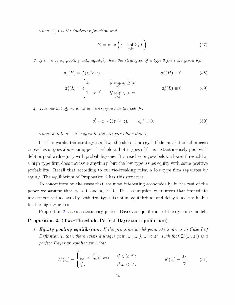
Proposition 2. (Two-Threshold Perfect Bayesian Equilibrium)

1. Equity pooling equilibrium. If the primitive model parameters are as in Case I of

Definition 1, then there exists a unique pair (z∗, z∗), z∗ < z∗, such that Ξe(z∗, z∗) is a

perfect Bayesian equilibrium with:

λ∗(zt) =

IrµH+k−µH/(1+ezt )

, if zt ≥ z∗;

Irk, if zt < z∗;

c∗(zt) =Ir

γ. (51)

24

In this equilibrium, debt is never issued and z∗ > zd/e.

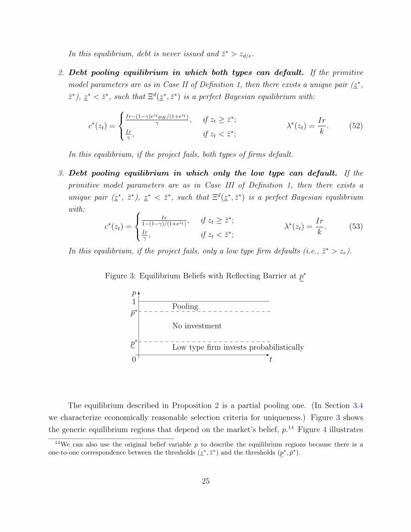
2. Debt pooling equilibrium in which both types can default. If the primitive

model parameters are as in Case II of Definition 1, then there exists a unique pair (z∗,

z∗), z∗ < z∗, such that Ξd(z∗, z∗) is a perfect Bayesian equilibrium with:

c∗(zt) =

Ir−(1−γ)eztµH/(1+ezt )

γ, if zt ≥ z∗;

Irγ, if zt < z∗;

λ∗(zt) =Ir

k. (52)

In this equilibrium, if the project fails, both types of firms default.

3. Debt pooling equilibrium in which only the low type can default. If the

primitive model parameters are as in Case III of Definition 1, then there exists a

unique pair (z∗, z∗), z∗ < z∗, such that Ξd(z∗, z∗) is a perfect Bayesian equilibrium

with:

c∗(zt) =

Ir1−(1−γ)/(1+ezt )

, if zt ≥ z∗;

Irγ, if zt < z∗;

λ∗(zt) =Ir

k. (53)

In this equilibrium, if the project fails, only a low type firm defaults (i.e., z∗ > zr).

Figure 3: Equilibrium Beliefs with Reflecting Barrier at p∗

6

-

p

t

p∗

p∗1

0

Pooling

No investment

Low type firm invests probabilistically

The equilibrium described in Proposition 2 is a partial pooling one. (In Section 3.4

we characterize economically reasonable selection criteria for uniqueness.) Figure 3 shows

the generic equilibrium regions that depend on the market’s belief, p.14 Figure 4 illustrates

14We can also use the original belief variable p to describe the equilibrium regions because there is aone-to-one correspondence between the thresholds (z∗, z∗) and the thresholds (p∗, p∗).

25

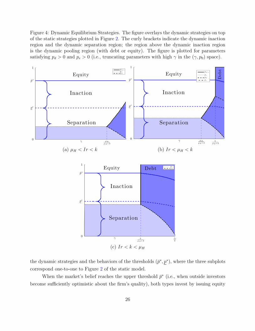
Figure 4: Dynamic Equilibrium Strategies. The figure overlays the dynamic strategies on topof the static strategies plotted in Figure 2. The curly brackets indicate the dynamic inactionregion and the dynamic separation region; the region above the dynamic inaction regionis the dynamic pooling region (with debt or equity). The figure is plotted for parameterssatisfying pd > 0 and pe > 0 (i.e., truncating parameters with high γ in the (γ, p0) space).

γ µH

µH+ k

0

p∗

p∗

1

Equity

Inaction

Separation

p d / ep ep d

γ µH

µH+ kk

µH+ k

0

p∗

p∗

1

Equity

Deb

t

Inaction

Separation

p d / e

p e

p d

p r

(a) µH < Ir < k (b) Ir < µH < k

γ kµH+ k

I rk

0

p∗

p∗

1Equity Debt

Inaction

Separation

p ep d

(c) Ir < k < µH

the dynamic strategies and the behaviors of the thresholds (p∗, p∗), where the three subplots

correspond one-to-one to Figure 2 of the static model.

When the market’s belief reaches the upper threshold p∗ (i.e., when outside investors

become sufficiently optimistic about the firm’s quality), both types invest by issuing equity

26

or debt. The upper barrier p∗ is essentially chosen by a high type firm to maximize its

value; a low type firm always imitates the high type. The trade-off between equity and

debt, conditional on investment, is similar to that in the static setting. For a fixed NPV, a

higher probability of success γ favors debt, whereas a lower γ favors equity. The debt coupon

also depends on whether a high type firm defaults upon project failure. Holding the NPV

fixed, conditional on equity issuance, the upper threshold p∗ does not vary with γ; however,

conditional on debt issuance, p∗ varies with γ.

When the market’s belief reaches p∗, only a low type firm invests. By (46) and (49),

it does so probabilistically. The lower barrier is chosen so that a low type firm is indifferent

between investing now (and thus revealing its type) and postponing investing with the hope

that positive shocks would lead the market’s belief to hit the upper boundary p∗ in the

future. The equilibrium rate of mixing by a low type firm at the lower boundary forces the

beliefs to be reflecting. That is, conditional on not observing investment at p∗, the market’s

belief immediately adjusts upwards, because a high type firm would never invest at the low

threshold. By (46) and (49), we can verify that in the equilibrium, zt is indeed the reflected

version of Zt at z∗:

zt = Zt + Yt = Zt + max

(z∗ − inf

s≤tZs, 0

). (54)

For all the market belief levels between the two thresholds, p∗ and p∗, there is a region of

optimal inaction in which both firm types postpone their decisions: a high type firm expects

the market’s belief to become more optimistic, which reduces underpricing, while a low type

firm speculates on positive shocks to its cash flows and higher overpricing of its (yet to be

issued) securities. This region of inaction is a new feature of the dynamic financing problem

and resembles the optimal economic behavior in many real option contexts, in which firms

face transaction costs of adjustment (e.g., see Stokey (2009)). The key difference from the

real option models is that delay in our models comes entirely from time-varying information

asymmetry.

The equilibrium thresholds (z∗, z∗) can be shown to be unique, but their expressions

are not in closed form. Nonetheless, the model is tractable enough to sign the comparative

statics with respect to the volatility level, σ. Volatility is an important parameter for the

dynamic model because it controls the accuracy of cash flow information and hence the firm’s

incentive to delay.

Proposition 3. (Behavior of Thresholds p∗ and p∗)

1. As σ → 0 and if the primitive model parameters are as in Proposition 2, then the

27

equilibrium thresholds p∗ → 1 and p∗ → 1/2.

2. As σ → +∞:

(a) If the primitive model parameters are as described in Part 1 of Proposition 2, then

the equilibrium thresholds p∗ → pe and p∗ → pe.

(b) If the primitive model parameters are as described in Parts 2 and 3 of Proposition

2, then the equilibrium thresholds p∗ → pd and p∗ → pd.

As discussed in Section 2, the thresholds pe and pd are strategically chosen by a high

type firm on the basis of the trade-off between investing in a positive NPV project and

reducing underpricing caused by asymmetric information about the assets in place. In the

dynamic setup, a high type firm can reduce the underpricing of assets by waiting and invest-

ing in the positive NPV project at a later date. As σ →∞, the realized cash flows become

increasingly uninformative, and investors can no longer learn the quality of assets over time.

Without learning, the dynamic environment is very similar to the static one of Section 2,

and the dynamic thresholds, p∗ and p∗, converge to the static threshold, pe or pd.

Conversely, as the cash flows become infinitely informative (i.e., as σ → 0), the true

type of the firm is revealed immediately. A high type firm sets the highest upper threshold

(i.e., p∗ → 1) to avoid underpricing. The less obvious limiting behavior of p∗ is the result of

two countervailing forces. On the one hand, a low type firm wishes to decrease its separation

threshold because pooling becomes more attractive. On the other hand, it wishes to increase

its separation threshold because a high type firm’s behavior implies a longer waiting time.

In equilibrium, these two forces exactly offset each other, making the lower threshold p∗

converge to 1/2.

3.3 Four-Threshold Equilibrium

In this subsection, we characterize a dynamic equilibrium for Cases IV–V of Definition 1. In

these regions of the model parameters, the volatility σ is “high” and the dynamic equilibrium

has a different structure: instead of two thresholds, it has four thresholds.

Before a formal analysis, it is useful to discuss intuitively why the two-threshold equi-

librium no longer applies for sufficiently high volatility. Consider, for example, Case I of

Definition 1, and increase σ. As σ increases, the benefits of waiting for a high type firm

deteriorate, because the cash flows become less informative. As the noisiness of cash flows

increases, the dynamic payoff VH(z) from following Ξe(z∗, z∗) of Proposition 2 decreases;

28

thus, so does the upper threshold, z∗. In the limiting case, as σ →∞, there is no incentive

to delay, so the region of investment should be exactly the same as in the static equilibrium.

It is tempting to conclude, by the argument of continuity, that the dynamic equilibrium

should be similar to the static one, at least qualitatively. This conclusion, however, does

not hold. Lemma 4 shows that there is an important discontinuity point within the static

investment region, at which a high type firm always delays investment for any finite σ.

Lemma 4. Suppose that market beliefs and the low type firm’s strategy are given by Ξe(z, z)

for some thresholds (z, z). If equity is the equilibrium security in the pooling region, a high

type firm never invests at zt = zd/e. If debt is the equilibrium security in the pooling region,

a high type firm never invests at zt = zr.

The technical reason behind Lemma 4 is that a high type firm’s static value function

has a kink at zt = zd/e (the threshold between risky debt and equity) and at zt = zr (the

threshold between relatively risky debt and relatively safe debt). At zt = zd/e, for example, a

high type firm prefers to wait and get an average of EeH(zd/e+ε) and Ed

H(zd/e−ε), rather than

collect EeH(zd/e) = Ed

H(zd/e) immediately. Therefore, regardless of σ, there exists an inaction

region around zd/e, as long as issuing equity is the equilibrium strategy for zt sufficiently

above zd/e. Similarly, a high type firm does not invest at zt = zr as long as issuing debt

on which a high type firm never defaults is the equilibrium strategy for the values of zt

sufficiently above zr.

What does Lemma 4 say about the structure of the dynamic equilibrium? Intuitively,

it implies that for sufficiently high σ, p = pd/e (or p = pr) can separate the investment regions

into two, generating a new inaction region around p = pd/e (or p = pr). This gives rise to a

four-threshold equilibrium, as characterized in Proposition 4.

Proposition 4. (Four-Threshold Perfect Bayesian Equilibrium)

1. Debt and Equity Pooling. If the primitive model parameters are as in Case IV of

Definition 1, there exists a unique four-tuple (z∗, z∗l , z∗h, z∗), where z∗ < z∗l < z∗h < z∗,

such that the following is a perfect Bayesian equilibrium:

(a) The strategies of a type θ firm are given by:

πdt (H) = 1(zt ∈ [z∗l , z∗h]), πet (H) = 1(zt ≥ z∗); (55)

πdt (L) = (1− πet−(L)) · 1(zt ∈ [z∗l , z∗h]), πet (L) =

1, if zt ≥ z∗;

1− e−Yt , if zt < z∗;(56)

29

where Yt = max

(z∗ − inf

s≤tZs, 0

).

(b) The market demands a share λ∗(zt) of the firm’s equity or a perpetuity with coupon

c∗(zt), where λ∗(zt) and c∗(zt) are given by:

λ∗(zt) =

IrµH+k−µH/(1+ezt )

, if zt ≥ z∗;

Ir/k, if zt < z∗;c∗(zt) =

Ir−(1−γ)eztµH/(1+ezt )

γ, if zt ∈ [z∗l , z

∗h];

Ir/γ, if zt /∈ [z∗l , z∗h];

(57)

with corresponding beliefs:

qet = pt · 1(zt ≥ z∗), qdt = pt · 1(zt ∈ [z∗l , z∗h]). (58)

In this equilibrium, z∗h < zd/e < z∗.

2. Debt Pooling. If the primitive model parameters are as in Case V of Definition 1,

there exists a unique four-tuple (z∗, z∗l , z∗h, z∗), where z∗ < z∗l < z∗h < z∗, such that the

following is a perfect Bayesian equilibrium:

(a) The strategies of a type θ firm are given by:

πdt (H) = 1(zt ∈ [z∗l , z∗h] or zt ≥ z∗), πet (H) ≡ 0; (59)

πdt (L) = (1− πet−(L)) · 1(zt ∈ [z∗l , z∗h] or zt ≥ z∗), πet (L) = 1− e−Yt , if zt < z∗;

(60)

where Yt = max

(z∗ − inf

s≤tZs, 0

).

(b) The market demands a share λ∗(zt) of firm’s equity or a perpetuity with coupon

c∗(zt):

λ∗(zt) = Ir/k, c∗(zt) =

Ir

1−(1−γ)/(1+ezt ), if zt ≥ z∗;

Ir−(1−γ)eztµH/(1+ezt )γ

, if zt ∈ [z∗l , z∗h];

Ir/γ, otherwise ;

(61)

with corresponding beliefs

qet ≡ 0, qdt = pt · 1(zt ∈ [z∗l , z∗h] or zt ≥ z∗). (62)

30

In this equilibrium, z∗h < zr < z∗.

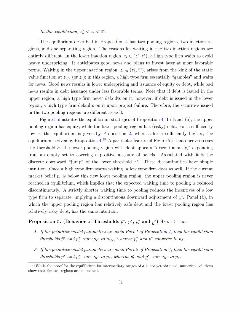
The equilibrium described in Proposition 4 has two pooling regions, two inaction re-

gions, and one separating region. The reasons for waiting in the two inaction regions are

entirely different. In the lower inaction region, zt ∈ (z∗, z∗l ), a high type firm waits to avoid

heavy underpricing. It anticipates good news and plans to invest later at more favorable

terms. Waiting in the upper inaction region, zt ∈ (z∗h, z∗), arises from the kink of the static

value function at zd/e (or zr); in this region, a high type firm essentially “gambles” and waits

for news. Good news results in lower underpricing and issuance of equity or debt, while bad

news results in debt issuance under less favorable terms. Note that if debt is issued in the

upper region, a high type firm never defaults on it; however, if debt is issued in the lower

region, a high type firm defaults on it upon project failure. Therefore, the securities issued

in the two pooling regions are different as well.

Figure 5 illustrates the equilibrium strategies of Proposition 4. In Panel (a), the upper

pooling region has equity, while the lower pooling region has (risky) debt. For a sufficiently

low σ, the equilibrium is given by Proposition 2, whereas for a sufficiently high σ, the

equilibrium is given by Proposition 4.15 A particular feature of Figure 5 is that once σ crosses

the threshold σ, the lower pooling region with debt appears “discontinuously,” expanding

from an empty set to covering a positive measure of beliefs. Associated with it is the

discrete downward “jump” of the lower threshold z∗. These discontinuities have simple

intuition. Once a high type firm starts waiting, a low type firm does as well. If the current

market belief pt is below this new lower pooling region, the upper pooling region is never

reached in equilibrium, which implies that the expected waiting time to pooling is reduced

discontinuously. A strictly shorter waiting time to pooling reduces the incentives of a low

type firm to separate, implying a discontinuous downward adjustment of z∗. Panel (b), in

which the upper pooling region has relatively safe debt and the lower pooling region has

relatively risky debt, has the same intuition.

Proposition 5. (Behavior of Thresholds p∗, p∗h, p∗l and p∗) As σ → +∞:

1. If the primitive model parameters are as in Part 1 of Proposition 4, then the equilibrium

thresholds p∗ and p∗h converge to pd/e, whereas p∗l and p∗ converge to pd.

2. If the primitive model parameters are as in Part 2 of Proposition 4, then the equilibrium

thresholds p∗ and p∗h converge to pr, whereas p∗l and p∗ converge to pd.

15While the proof for the equilibrium for intermediary ranges of σ is not yet obtained, numerical solutionsshow that the two regions are connected.

31

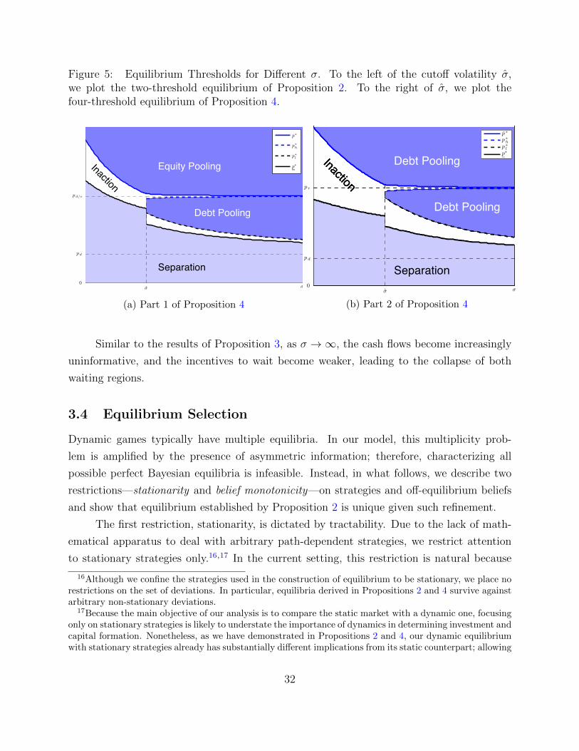
Figure 5: Equilibrium Thresholds for Different σ. To the left of the cutoff volatility σ,we plot the two-threshold equilibrium of Proposition 2. To the right of σ, we plot thefour-threshold equilibrium of Proposition 4.

! !0

p d

p d/e

Equity Pooling

Debt Pooling

Separation

Inaction

p!

p!h

p!l

p!

Student Version of MATLAB

(a) Part 1 of Proposition 4

Debt Pooling

Debt Pooling

Separation

Inaction

Debt Pooling

Debt Pooling

Separation

Inaction

! !0

p d

p r

Debt Pooling

Debt Pooling

Separation

Inaction

p!

p!h

p!l

p!

(b) Part 2 of Proposition 4

Similar to the results of Proposition 3, as σ →∞, the cash flows become increasingly

uninformative, and the incentives to wait become weaker, leading to the collapse of both

waiting regions.

3.4 Equilibrium Selection

Dynamic games typically have multiple equilibria. In our model, this multiplicity prob-

lem is amplified by the presence of asymmetric information; therefore, characterizing all

possible perfect Bayesian equilibria is infeasible. Instead, in what follows, we describe two

restrictions—stationarity and belief monotonicity—on strategies and off-equilibrium beliefs

and show that equilibrium established by Proposition 2 is unique given such refinement.

The first restriction, stationarity, is dictated by tractability. Due to the lack of math-

ematical apparatus to deal with arbitrary path-dependent strategies, we restrict attention

to stationary strategies only.16,17 In the current setting, this restriction is natural because

16Although we confine the strategies used in the construction of equilibrium to be stationary, we place norestrictions on the set of deviations. In particular, equilibria derived in Propositions 2 and 4 survive againstarbitrary non-stationary deviations.

17Because the main objective of our analysis is to compare the static market with a dynamic one, focusingonly on stationary strategies is likely to understate the importance of dynamics in determining investment andcapital formation. Nonetheless, as we have demonstrated in Propositions 2 and 4, our dynamic equilibriumwith stationary strategies already has substantially different implications from its static counterpart; allowing

32

the dynamics of our model are driven by the time-homogeneous Markov cash flow process

Xtt≥0.

Definition 4. (Stationary Equilibrium) An equilibrium is stationary if:

(i) The market belief p is a time-homogeneous Markov process; and

(ii) The market pricing rules λ∗ and c∗ are functions of pt only.

Stationarity substantially shrinks the set of possible equilibria by placing restrictions

on strategies along the equilibrium path. Off the equilibrium path, however, stationarity has

limited power and does not eliminate economically unreasonable beliefs. For example, if the

market “threatens” the firm that it believes the firm is of the low type with probability 1 if

there is no issuance at t = 0, we are back to the static equilibrium. Such beliefs, however, fail

the following intuitive forward induction reasoning: if the market does not observe equity

issuance at t = 0, this deviation is more likely to be caused by a high type firm (because a

low type firm always prefers to invest under any belief). This reasoning suggests that the

market’s conditional probability that the firm is of the high type, pt, should increase right

after t = 0, if there is no issuance. This, in turn, creates incentives for a low type firm to

delay investment.

To exclude such economically unreasonable equilibria, we require beliefs to be mono-

tone. This refinement is a natural extension of the Divinity refinement (Banks and Sobel

(1987)) to the continuous-time setting and has been used by Daley and Green (2012) and

Gul and Pesendorfer (2012).

Definition 5. (Monotone Beliefs) A belief process p is monotone if for all t > s:

pt ≥ϕHt−s(Xt −Xs)ps

ϕHt−s(Xt −Xs)ps + ϕLt−s(Xt −Xs)(1− ps). (63)

Notice that if we replace p with P in (63), it would hold with equality. In other words,

the belief monotonicity condition requires the market belief pt to be at least as high as a

non-strategic posterior Pt, given that they start from the same point, Ps = ps, in the absence

of issuance between s and t. Hence, the investment delay is interpreted as a signal, which is

more likely to be sent by a high type firm.

Stationarity, together with competitiveness of the market, implies that at any moment

in time only one of the two offers (λt, ct) from the market is relevant: either the offer selected

nonstationary, time-dependent strategies is likely to make the difference starker.

33

by a high type firm (and hence also by a low type firm) or the equity offer selected only

by a low type firm. The former case corresponds to a pooling equilibrium, while the latter

corresponds to the separating equilibrium. Such behavior implies that (63) is satisfied along

the equilibrium path. The monotone-beliefs refinement requires that this condition hold off

the equilibrium path as well.

Both the four-threshold and two-threshold equilibria introduced earlier are station-

ary and satisfy belief monotonicity. Proposition 6 shows the uniqueness of equilibrium in

Proposition 2, given the two refinements discussed above.

Proposition 6. (Equilibrium Uniqueness) If primitive model parameters are as stated in

Proposition 2, then the equilibrium of Proposition 2 is the unique stationary perfect Bayesian

equilibrium with monotone belief process p.

Thus, the equilibrium derived in Proposition 2 is the only reasonable equilibrium within

a broad class of equilibria that admit only stationary strategies.18 Instead of proving this

result directly, we refer readers to Daley and Green (2012)’s Theorem 5.1. Using essentially

the same technique, one could show that the uniqueness of the equilibrium in their model

implies the uniqueness of the equilibrium for parametric cases of Proposition 2. While the

uniqueness proof is similar, we note again that the equilibrium of Daley and Green (2012)

is essentially equity-only and does not consider debt.

3.5 Extension: Stochastic Decay of the Investment Opportunity

So far in our analysis, either the project evaporates immediately if not taken at time zero,

or it does not evaporate at all. In reality, however, the firm cannot delay the investment

decision indefinitely. The project could become unavailable or infeasible for a wide variety of

reasons, including technology becoming obsolete, competitors gaining a first-mover advan-

tage, or regulatory intervention. In this section, we model the rate of decay of the investment

opportunity and study its effect on the dynamic equilibrium.

Suppose that the investment option evaporates with time-invariant intensity, δ > 0.

That is, conditional on no investment up to time t, the project evaporates with probability

δdt in the next instance of time, dt; it remains available at time t + dt with probability

1− δdt. The static model of Section 2 corresponds to one extreme case of δ = +∞ and the

dynamic model of this section so far corresponds to the other extreme case, δ = 0.

18Proposition 6 also holds for a more general definition of strategies that includes off-equilibrium behavior.The resulting equilibrium is equivalent to the one described in Proposition 2 on the equilibrium path.

34

Proposition 7 characterizes the dynamic equilibrium with a stochastic decay.

Proposition 7. (Stochastic Decay) Given the primitive model parameters and δ > 0,

define:

σ = σ

√1 +

δ

r. (64)

Then, the dynamic equilibrium with (σ, δ) is equivalent to the dynamic equilibrium with σ

and δ = 0 characterized in Propositions 2 and 4.

The introduction of a positive rate of decay reduces the incentives to delay investment

for both types of firms. Intuitively, an increase in δ has a similar effect on the equilibrium

strategies as an increase in σ does, since the latter makes it more difficult for the market to

separate the two firm types based on the observed cash flows, which reduces the option value

to wait. Proposition 7 makes this intuition precise and shows that by properly adjusting the

volatility of the cash flows, one can compute the equilibrium with a stochastic decay based

on the equilibrium with an infinitely lived project. In light of this result, the comparative

statics with respect to δ have the same sign as those with respect to σ.

4 Discussion

In this section, we explore the economic implications of the dynamic equilibrium and compare

them to the implications of the static equilibrium of Myers and Majluf (1984). We first

examine the effect of dynamics on social welfare. Then, we discuss the empirical implications

of our results, including firm market values, investment delay, and security choices, among

others.

4.1 Firm Values and Social Welfare

In the static market, adverse selection can lead to a welfare loss because a high type firm

forgoes a positive-NPV project because of the low market prices of its securities. In the

dynamic market, the project is eventually implemented, but the welfare loss comes from the

endogenous delay by both types of firms. In this subsection, we explore the net welfare effect

of delayed investment.

As a first step, we analyze the private benefits and costs of the two types of firms.

For the purpose of this section, we let Eθ(p) and Vθ(p) be the values of a type θ firm (i.e.,

its existing shareholders), given the belief p, in the static and dynamic models, respectively.

35

The dynamic value function Vθ is given by Proposition 2 or Proposition 4, depending on the

primitive model parameters. Proposition 8 compares firm values in both environments.

Proposition 8. (Static and Dynamic Firm Values) The values of the firm’s existing

shareholders, Eθ(p) and Vθ(p), satisfy the following:

1. For a high type firm:

(a) VH(p) = EH(p) in the dynamic pooling region;

(b) VH(p) > EH(p) in the dynamic inaction region.

2. For a low type firm:

(a) VL(p) = EL(p) in the dynamic pooling region and in the intersection between the

dynamic and static separating regions;

(b) VL(p) < EL(p) in the intersection between the dynamic inaction region and the

static pooling region;

(c) VL(p) > EL(p) in the intersection between the dynamic inaction region and the

static separating region.

A high type firm never prefers the static world, because it gains from an option to

delay. It is a high type firm that effectively chooses the lower boundary of the dynamic

pooling region. The value of waiting is zero if market belief is very high, in which case

immediate investment is optimal anyway. The low type firm’s preference is slightly subtler.

If the market belief is very high or very low, the dynamic equilibrium dictates immediate

investment, either by pooling or separation. In this case, investment delay has zero value.

If delay allows a low type firm to avoid separation, delay has a positive value. If, however,

delay prevents immediate pooling by a low type firm with the high type, then the option

to delay harms a low type firm. The last case occurs under an intermediate belief of the

market, which is arguably the most interesting case. Therefore, the net welfare implications

of options to delay become ambiguous, as delay benefits the high type firm and harms the

low type firm.

To study the net effect of the delay option, we let E and V be the unconditional firm

values in the static and the dynamic economies, respectively. That is, E(p) = pEH(p) + (1−p)EL(p) and V (p) = pVH(p) + (1− p)VL(p). These values summarize the social welfare, and

a comparison between them enables us to explore welfare implications. Proposition 9 shows

that adding dynamics does not always lead to a higher social welfare.

36

Proposition 9. (Static and Dynamic Social Welfare) The unconditional firm values,

E(p) and V (p), satisfy the following:

1. V = E in the dynamic pooling regions;

2. V > E in the static separation region;

3. V < E in the intersection between the dynamic inaction region and the static pooling

region.

In the separation region of the static world, a high type firm never invests. Thus,

allowing delay leads to eventual investment and improves welfare. In the intersection between

the dynamic inaction region and the static pooling region, immediate investment is first best.

Allowing delay in this case reduces welfare because of the lost time value of money. In other

words, the delay is inefficient from the social planner’s point of view.

The result that delay can lead to a welfare loss may hinge, of course, on the specific

economic structure we consider. For example, one may reasonably suspect that high-quality

firms in practice would scale down investments if they are perceived as low quality and

suffer from underpricing. If delay improves market belief and leads to a larger positive-NPV

project, welfare may be improved. We leave this and other alternative specifications to future

research.

4.2 Empirical Implications

Our model has a number of empirical implications.

Pecking Order and Project Risk. Both our static and dynamic equilibria predict that

conditional on the same NPV, a safer project (i.e., more likely to succeed) is more likely

to be financed by debt, while a riskier one is more likely to be financed by equity. This

result is not driven by risk aversion (all agents in our model are risk-neutral) or default

costs (default incurs no deadweight costs in our model). Instead, it stems from the trade-off

between underpricing of securities and the loss of assets in place in default. Even though

debt is less sensitive to private information, a high probability of default can force a high

type firm to issue equity and a low type firm to follow.

Investment and Negative News. Our model predicts that investments can take place

even after a series of bad news. Such behavior arises either because of the separation by the

37

low type firm, or if the lower pooling region is reached (see Proposition 4). The two scenarios

are governed by different mechanisms and produce distinct implications for equity prices.

If a low type firm invests at the lower threshold z∗, it does so because of dim prospects

of pooling with the high type firm and issuing overpriced securities to finance investments.

Thus, investment is financed by new equity issuance, revealing the type of the firm to the

market. Therefore, the theory predicts a negative impact of secondary equity offerings on

the equity price above and beyond the informational content of the unfavorable news.

If the lower pooling region (z∗l , z∗h) is reached from above, both firm types invest using

debt financing. Such investment behavior provides no additional information to the market

because both the high type firm and the low type firm invest at that point. Therefore, our

model predicts that new debt issuance after bad news has no discernible impact on the equity

price above and beyond the informational content of the negative news before investments.

Investment and Positive News. As positive news arrives over time, the market becomes

increasingly optimistic about the firm’s type and improves its financing terms (lower interest

rates for debt and higher equity price). With cheaper financing, one may expect the firm to

undertake more investments. However, this is not always the case in our model. Conditional

on the same pool of investment opportunities, a firm with more volatile cash flows is less

likely to invest in response to an increase in market beliefs as compared to a less volatile firm.

This difference in behavior stems from the presence of the upper inaction region for some

primitive model parameters and a high σ, which leads to delayed investment (Proposition

4).

Security Choice and Announcement Returns. Our results predict that the abnormal

stock returns upon debt issuance should be zero. This is because debt is a pooling security

in our equilibrium. By contrast, equity issuance should be followed by negative abnormal

stock returns because the low-type firm separates by equity. Although separation by equity

is imposed by the tie-breaking rule in our model, this choice is robust to the introduction of

distress cost.

Quality of Information and Security Choice. We also predict that an increase in

the quality of the information available to the market weakly increases the probability of

equity issuance and weakly decreases the probability of debt issuance. In our model, as cash

flows become increasingly more informative, the four-threshold equilibrium no longer exists.

Because the lower pooling region in the four-threshold equilibrium always has debt issuance,

38

a higher informativeness of cash flows tilts the equilibrium towards more equity issuance and

less debt issuance in expectation.

5 Conclusion

In this paper, we reexamine the classic yet static model of Myers and Majluf (1984) in a

dynamic environment. Firms can optimally delay investment decisions in an attempt to

signal their quality, while the market learns about firms’ qualities by observing the noisy

cash flows generated from their assets in place. In a two-threshold equilibrium, a high-

quality firm optimally delays investment, balancing the trade-off between the underpricing

of its securities and the lost time value of project NPV. A low-quality firm imitates the high

quality firm as much as possible, but upon a series of sufficiently bad cash flows, the low-

quality firm invests probabilistically and separates itself. Unlike in the static equilibrium of

Myers and Majluf (1984), in our model, investment eventually takes place.

We also characterize firms’ optimal choice between debt and equity in this dynamic

model, building on the pecking order theory of Myers (1984). We show that if the new project

can fail with a sufficiently high probability, a high-quality firm can have a higher cost of losing

the existing assets upon debt default than the underpricing of its equity. Therefore, for a

given project NPV, relatively safe projects favor debt, whereas relatively risky projects favor

equity. This partial violation of the pecking order is consistent with empirical evidence that

small, high-growth firms prefer equity over debt.

The combination of security choices and the option to delay leads to a new type of

four-threshold equilibrium, which features two pooling regions with different securities, two

inaction regions, and one separation region. The choice between debt and equity introduces

a kink in the static value function. At this kink, investing immediately is never optimal,

and the firm would rather “wait and see” before deciding the security type. Therefore, the

four-threshold equilibrium is qualitatively different from our two-threshold equilibrium with

a single security and Daley and Green (2012)’s (essentially) equity-only equilibrium.

39

Appendix

A List of Model Variables

Variable Description

Variables introduced in Section 2 (static model)

θ ∈ H,L Type of the firm(Xθ

t )t≥0 Cumulative cash flow process of type θ firmµθ Drift of the cash flow process Xθ

σ Instantaneous volatility of Xθ

K Increase in instantaneous cash flow rate if new production technologysucceeds

γ Success probability of the new production technologyk = γK Expected increase in instantaneous cash flow rate due to new technol-

ogyr Risk-free rateI Cost of adopting new technologyp0 Prior probability of θ = Hλ Fraction of the company demanded by the marketc Perpetuity coupon demanded by the marketπe(θ) = πe(θ;λ, c) Probability of equity issuance by type θ firm given market offers (λ, c)πd(θ) = πd(θ;λ, c) Probability of debt issuance by type θ firm given market offers (λ, c)E∅θ Expected equity value of old shareholders for not making investmentEeθ(λ) Expected equity value of old shareholders for investing with equity

financingEeθ(c) Expected equity value of old shareholders for investing with debt fi-

nancingSe(λ, c) Expected payoff to the market from buying equity given offers (λ, c)Sd(λ, c) Expected payoff to the market from buying debt given offers (λ, c)qe0 Market belief about the quality of the type issuing equity at time 0qd0 Market belief about the quality of the type issuing debt at time 0λ(qe0) A break-even equity offer λ given the belief qe0c(qd0) A break-even debt offer c given the belief qd0pe Belief threshold solving Ee

H(λ(pe)) = E∅Hpd Belief threshold solving Ed

H(c(pe)) = E∅Hpd/e Belief threshold solving Ee

H(λ(pd/e)) = EdH(c(pd/e))

pr Belief threshold solving c(pr) = µHContinued on next page

40

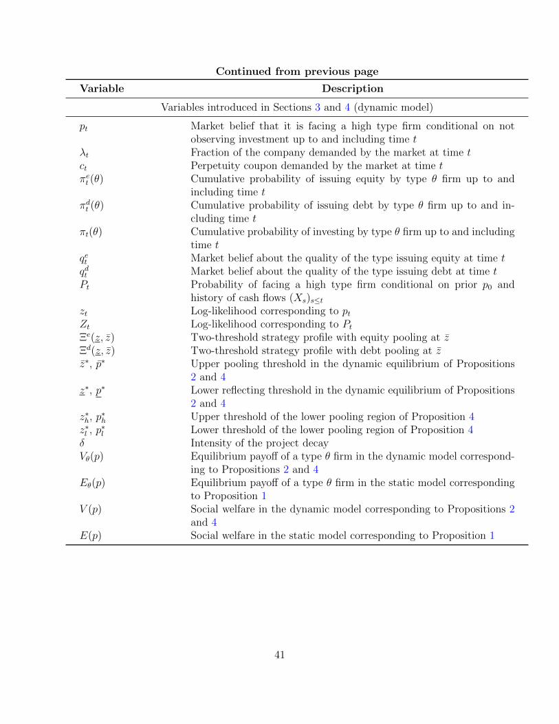
Continued from previous page

Variable Description

Variables introduced in Sections 3 and 4 (dynamic model)

pt Market belief that it is facing a high type firm conditional on notobserving investment up to and including time t

λt Fraction of the company demanded by the market at time tct Perpetuity coupon demanded by the market at time tπet (θ) Cumulative probability of issuing equity by type θ firm up to and

including time tπdt (θ) Cumulative probability of issuing debt by type θ firm up to and in-

cluding time tπt(θ) Cumulative probability of investing by type θ firm up to and including

time tqet Market belief about the quality of the type issuing equity at time tqdt Market belief about the quality of the type issuing debt at time tPt Probability of facing a high type firm conditional on prior p0 and

history of cash flows (Xs)s≤tzt Log-likelihood corresponding to ptZt Log-likelihood corresponding to PtΞe(z, z) Two-threshold strategy profile with equity pooling at zΞd(z, z) Two-threshold strategy profile with debt pooling at zz∗, p∗ Upper pooling threshold in the dynamic equilibrium of Propositions

2 and 4z∗, p∗ Lower reflecting threshold in the dynamic equilibrium of Propositions

2 and 4z∗h, p

∗h Upper threshold of the lower pooling region of Proposition 4

z∗l , p∗l Lower threshold of the lower pooling region of Proposition 4

δ Intensity of the project decayVθ(p) Equilibrium payoff of a type θ firm in the dynamic model correspond-

ing to Propositions 2 and 4Eθ(p) Equilibrium payoff of a type θ firm in the static model corresponding

to Proposition 1V (p) Social welfare in the dynamic model corresponding to Propositions 2

and 4E(p) Social welfare in the static model corresponding to Proposition 1

41

B Proofs and Details

B.1 Proof of Lemma 3

Consider first the case where the min(·) in (26) is equal to µHr

, i.e. q0 < pr. The comparisonbetween (25) and (26) boils down to:

EeH(λ(q0)) vs. Ed

H(C(q0)) (B1)

(1− q0)(1− γ)µHr

vs. (1− q0)IµH

q0µH + k(B2)

1− γr

vs.I

q0µH + k(B3)

q0µH + k vs.Ir

1− γ(B4)

q0 vs.1

µH

(Ir

1− γ− k)≡ pd/e. (B5)

Thus, if q0 is above pd/e, then equity dominates risky debt for the high type firm; ifq0 < pd/e, risky debt dominates equity. This concludes the proof of statements 1(a) and 2(a)of Lemma 3.

Consider the situation when the high type firm’s debt is riskless (i.e., q0 > pr). Then,the trade-off is:

EeH(λ(q0)) vs. Ed

H(C(q0)) (B6)

(1− q0)(1− γ)I

1− (1− γ)(1− q0)vs. (1− q0)I

µHq0µH + k

(B7)

1− γ1− (1− γ)(1− q0)

vs.µH

q0µH + k(B8)

k

k + µHvs. γ. (B9)

It turns our that the comparison between riskless debt and equity for the high typefirm does not depend on the level of market belief, q0. Debt dominates equity if γ > k

k+µH,

and equity dominates debt if γ < kk+µH

.

B.2 Proof of Proposition 1

First, one can easily strengthen the results of Lemmas 1 and 2 and conclude that:

EeL(λ(qe0)) ≥ µL

r+

(k

r− I), ∀ qe0 ∈ [0, 1] and Ed

L(C(qd0)) ≥ µLr

+

(k

r− I), ∀ qd0 ∈ [0, 1].

(B10)The above inequalities imply that the low type firm is always willing to pool with the

42

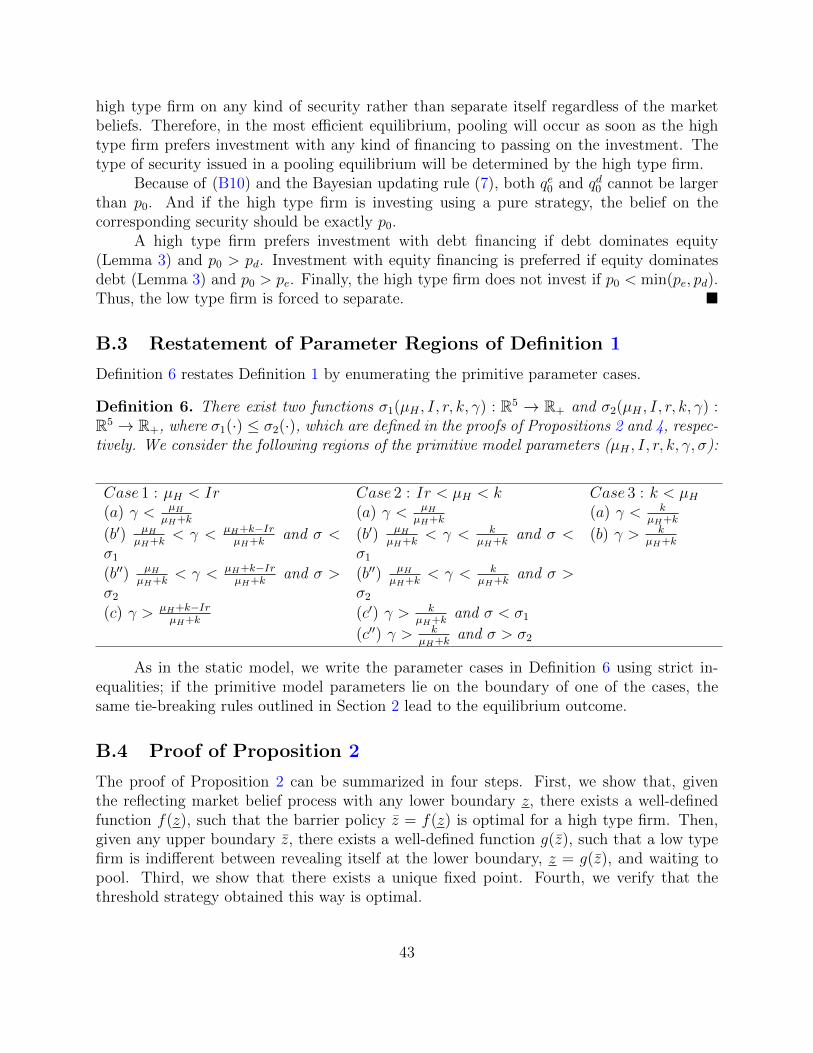
high type firm on any kind of security rather than separate itself regardless of the marketbeliefs. Therefore, in the most efficient equilibrium, pooling will occur as soon as the hightype firm prefers investment with any kind of financing to passing on the investment. Thetype of security issued in a pooling equilibrium will be determined by the high type firm.

Because of (B10) and the Bayesian updating rule (7), both qe0 and qd0 cannot be largerthan p0. And if the high type firm is investing using a pure strategy, the belief on thecorresponding security should be exactly p0.

A high type firm prefers investment with debt financing if debt dominates equity(Lemma 3) and p0 > pd. Investment with equity financing is preferred if equity dominatesdebt (Lemma 3) and p0 > pe. Finally, the high type firm does not invest if p0 < min(pe, pd).Thus, the low type firm is forced to separate.

B.3 Restatement of Parameter Regions of Definition 1

Definition 6 restates Definition 1 by enumerating the primitive parameter cases.

Definition 6. There exist two functions σ1(µH , I, r, k, γ) : R5 → R+ and σ2(µH , I, r, k, γ) :R5 → R+, where σ1(·) ≤ σ2(·), which are defined in the proofs of Propositions 2 and 4, respec-tively. We consider the following regions of the primitive model parameters (µH , I, r, k, γ, σ):

Case 1 : µH < Ir Case 2 : Ir < µH < k Case 3 : k < µH(a) γ < µH

µH+k(a) γ < µH

µH+k(a) γ < k

µH+k

(b′) µHµH+k

< γ < µH+k−IrµH+k

and σ <σ1

(b′) µHµH+k

< γ < kµH+k

and σ <σ1

(b) γ > kµH+k

(b′′) µHµH+k

< γ < µH+k−IrµH+k

and σ >σ2

(b′′) µHµH+k

< γ < kµH+k

and σ >σ2

(c) γ > µH+k−IrµH+k

(c′) γ > kµH+k

and σ < σ1

(c′′) γ > kµH+k

and σ > σ2

As in the static model, we write the parameter cases in Definition 6 using strict in-equalities; if the primitive model parameters lie on the boundary of one of the cases, thesame tie-breaking rules outlined in Section 2 lead to the equilibrium outcome.

B.4 Proof of Proposition 2

The proof of Proposition 2 can be summarized in four steps. First, we show that, giventhe reflecting market belief process with any lower boundary z, there exists a well-definedfunction f(z), such that the barrier policy z = f(z) is optimal for a high type firm. Then,given any upper boundary z, there exists a well-defined function g(z), such that a low typefirm is indifferent between revealing itself at the lower boundary, z = g(z), and waiting topool. Third, we show that there exists a unique fixed point. Fourth, we verify that thethreshold strategy obtained this way is optimal.

43

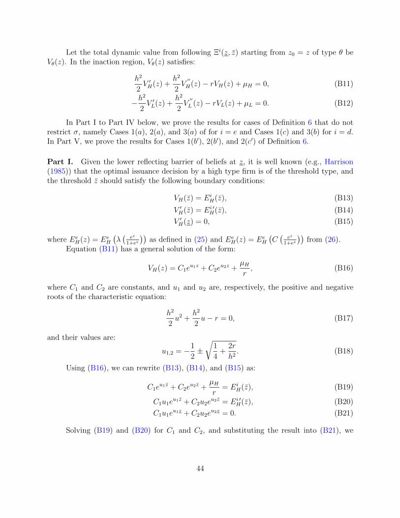
Let the total dynamic value from following Ξi(z, z) starting from z0 = z of type θ beVθ(z). In the inaction region, Vθ(z) satisfies:

h2

2V ′H(z) +

h2

2V′′

H(z)− rVH(z) + µH = 0, (B11)

−h2

2V ′L(z) +

h2

2V′′

L (z)− rVL(z) + µL = 0. (B12)

In Part I to Part IV below, we prove the results for cases of Definition 6 that do notrestrict σ, namely Cases 1(a), 2(a), and 3(a) of for i = e and Cases 1(c) and 3(b) for i = d.In Part V, we prove the results for Cases 1(b′), 2(b′), and 2(c′) of Definition 6.

Part I. Given the lower reflecting barrier of beliefs at z, it is well known (e.g., Harrison(1985)) that the optimal issuance decision by a high type firm is of the threshold type, andthe threshold z should satisfy the following boundary conditions:

VH(z) = EiH(z), (B13)

V ′H(z) = Ei ′H(z), (B14)

V ′H(z) = 0, (B15)

where EeH(z) = Ee

H

(λ(

ez

1+ez

))as defined in (25) and Ee

H(z) = EeH

(C(

ez

1+ez

))from (26).

Equation (B11) has a general solution of the form:

VH(z) = C1eu1z + C2e

u2z +µHr, (B16)

where C1 and C2 are constants, and u1 and u2 are, respectively, the positive and negativeroots of the characteristic equation:

h2

2u2 +

h2

2u− r = 0, (B17)

and their values are:

u1,2 = −1

2±√

1

4+

2r

h2. (B18)

Using (B16), we can rewrite (B13), (B14), and (B15) as:

C1eu1z + C2e

u2z +µHr

= EiH(z), (B19)

C1u1eu1z + C2u2e

u2z = Ei ′H(z), (B20)

C1u1eu1z + C2u2e

u2z = 0. (B21)

Solving (B19) and (B20) for C1 and C2, and substituting the result into (B21), we

44

obtain:

e(u1−u2)z = −u2

u1

u1(EiH(z)− µH/r)− Ei ′

H(z)

Ei ′H(z)− u2(Ei

H(z)− µH/r)· e(u1−u2)z. (B22)

As we prove below, the right-hand side (RHS) of (B22) is strictly increasing in z.Together with the limiting values and the implicit function theorem, this would imply theexistence of a continuous and strictly increasing function, f(z).

The partial derivative of the RHS of (B22) w.r.t. z is equal to (up to a positivemultiplier):

(u1 − u2)u1(Ei

H(z)− µH/r)− Ei ′H(z)

Ei ′H(z)− u2(Ei

H(z)− µH/r)

+(u1E

i ′H(z)− Ei ′′

H (z)(Ei ′H(z)− u2(Ei

H(z)− µH/r))(Ei ′

H(z)− u2(EiH(z)− µH/r))2

− (u1(EiH(z)− µH/r)− Ei ′

H(z))(Ei ′′H (z)− u2E

i ′H(z))

(Ei ′H(z)− u2(Ei

H(z)− µH/r))2.

(B23)

The second term of (B23) is positive because Ei ′H > 0, Ei ′′

H ≤ 0 (which can be seen bydifferentiating equations (25)–(26)), u2 < 0, and Ei

H(z)− µH/r > 0. For all z > zmin, wherezmin is a unique root of:

u1(EiH(zmin)− µH/r)− Ei ′

H(zmin) = 0. (B24)

The sign of the sum of the first and the third terms of (B23) is determined by the signof

(u1−u2)[Ei ′H−u2(Ei

H−µH/r)]− [Ei ′′H −u2E

i ′H ] = u1E

i ′h −u2(u1−u2)(Ei

H−µH/r)−Ei ′′H > 0.(B25)

As z → +∞, the RHS of (B22) also approaches +∞.Hence, for any z there exists a well-defined, smooth, and strictly increasing best re-

sponse function z = f(z).

Part II. Next, we solve the problem for a low type firm. Given z and a reflecting beliefprocess at z, there exists a unique z, such that a low type firm is exactly indifferent at thelower boundary. Therefore, it randomizes to sustain the reflecting beliefs. Similar to theabove, (B12) has a general solution:

VL(z) = D1ev1z +D2e

v2z +µLr, (B26)

where D1 and D2 are constants, and v1 and v2 are, respectively, the positive and negativeroots of the characteristic equation:

h2

2v2 − h2

2v − r = 0, (B27)

45

and their values are:

v1,2 =1

2±√

1

4+

2r

h2. (B28)

The value function has to satisfy (see Harrison (1985)) three conditions: indifferenceand reflecting at the lower boundary, and value matching at the upper boundary:

VL(z) =µL + k

r− I, (B29)

V ′L(z) = 0, (B30)

VL(z) = EiL(z). (B31)

Using (B26), we can re-write (B29) and (B30) as:

D1ev1z +D2e

v2z +µLr

=µL + k

r− I, (B32)

D1v1ev1z +D2v2e

v2z = 0. (B33)

Solving (B32) and (B33) for D1 and D2, we can write D1 and D2 in terms of z:(D1

D2

)=

1

v1 − v2

(−v2e

(v2−1)z

v1e(v1−1)z

)(k

r− I). (B34)

Substituting (B34) into (B31), we obtain:

1

v1 − v2

(k

r− I)(

v1e(v1−1)z+v2z − v2e

(v2−1)z+v1z)

= EiL(z)− µL

r. (B35)

It suffices to show that for any given z there exists a unique z such that (B35) holds.The RHS of (B35) is not a function of z, while for the left-hand side (LHS):

d LHS

dz=

1

v1 − v2

(k

r− I)v1v2

(ev1(z−z) − ev2(z−z)) < 0, ∀z ≤ z. (B36)

Because v1 + v2 = 1, as z → z, LHS → kr− I < RHS, and as z → −∞, LHS →∞.

Thus, by the intermediate value theorem and monotonicity, we have a unique solution z =g(z) < z.

Part III. Re-writing (B35), using z = f−1(z), we obtain:

1

v1 − v2

(k

r− I)(

v1

(ez

ef−1(z)

)v2

− v2

(ez

ef−1(z)

)v1)−(EiL(z)− µL

r

)= 0. (B37)

Any root of this equation greater than zmin (defined in (B24)) gives rise to a pair (z, z)that characterizes an equilibrium. Here, z ≥ zmin is needed, because both sides of (B22)

46

must be positive.Notice that, as z → zmin+, the LHS of (B37) approaches +∞, because f−1(z), which

is a positive multiple of the log of the RHS of (B22), approaches −∞, and v1 > 0 > v2.By (B22), z − z → 0 as z →∞. Thus, as z → +∞, the limit of the LHS of (B37) is:(

k

r− I)−(EiL(z)− µL

r

)< 0. (B38)

The partial derivative of the LHS of (B37) is equal to:

v1v2

v1 − v2

(k

r− I)[(

ez

ef−1(z)

)v2−1

−(

ez

ef−1(z)

)v1−1]· ddz

(ez

ef−1(z)

)− Ei ′

L (z). (B39)

We already know that Ei ′L > 0, v1 > 0 > v2, and k

r− I > 0. Differentiating ez

ezfrom (B22),

we find that ddz

(ez

ef−1(z)

)< 0. Finally,

(ez

ef−1(z)

)v2−1

<(

ez

ef−1(z)

)v1−1

, because ez

ef−1(z)

> 1.

We have proved that the whole expression in (B39) is negative. Thus, the LHS of(B37) is strictly decreasing from +∞ at zmin+ to a negative value at +∞. Therefore, thereexists a unique z∗ > zmin that solves (B37). The other boundary z∗ is given by f−1(z∗) or,equivalently, by g(z∗).

Part IV. We have shown that the pair (z∗, z∗) constitutes a unique equilibrium, if we allowdeviations within the class of two threshold (lower reflective and upper pooling, respectively)strategies. However, it does not account for arbitrary deviations that are allowed by thedefinition of π(θ). We now verify the sub-optimality of arbitrary deviations by consideringa modified version of our game. Define V ∗θ (z) as the value function of the original game:

V ∗θ (z) = sup(πd,πe)

E

[∫ ∞0

(∫ t

0

e−rudXu

)d(πet + πdt ) +

∫ ∞0

e−rt(Eeθ(λ∗(qet )) dπ

et + Ed

θ (c∗(qdt )) dπdt

)].

(B40)Consider the following modification: at any moment the firm can be sold to an outsider

for Vθ(z), where Vθ is the expected payoff to a type θ player when the parties play Ξi(z∗, z∗)strategies.

Define Vθ(z) as be the value function of the modified game:

Vθ(z) = sup(πd,πe)

E

[∫ ∞0

(∫ t

0

e−rudXu

)d(πet + πdt ) (B41)

+

∫ ∞0

e−rt(max(Vθ(zt), E

eθ(λ∗(qet ))) dπ

et + max(Vθ(zt), E

dθ (c∗(qdt ))) dπ

dt

)].

Clearly, Vθ(z) ≥ V ∗θ (z) ≥ Vθ(z). In addition, Vθ(zt) ≥ Eiθ(zt), which can be easily seen

from equations (B13)–(B15) and (B29)–(B31), as well as debt coupon c∗ and equity shareλ∗ defined in (51)–(53). Moreover, in Cases 1(a), 2(a), 3(a), 1(c) or 3(b) of Definition 6,

47

EiH(zt) ≥ E−iH (zt), where −i denotes the security other than the equilibrium one.19 Hence,

VH(zt) ≥ E−iH (zt).For the low type firm, E−iL (·) ≡ µL

r+ k

r− I because using the off-equilibrium security

−i implies separation. Thus, E−iL (·) < VL(zt) and

Vθ(zt) ≥ max(Eeθ(λ∗(qet )), E

dθ (c∗(qdt ))

). (B42)

Therefore:

Vθ(z) = supπ(θ)

E

[∫ ∞0

(∫ t

0

e−rudXu + e−rtVθ(zt))dπt(θ)

]. (B43)

In this case, there is no need for mixed strategies, because every player is facing a simpleoptimal stopping problem. Thus, we can re-write V as:

Vθ(z) = supτ

E

[∫ τ

0

e−rudXu + e−rτVθ(zτ )

]= sup

τE[(1− e−rτ )µθ

r+ e−rτVθ(zτ )

]= sup

τE fθ(τ, zτ ).

(B44)

Because Vθ is in C2, except for the two points z∗, z∗, we can use Ito’s lemma andwrite:

dfθ(t, zt) = re−rtµθrdt− re−rtVθ(zt)dt+ e−rtdVθ(zt) (B45)

= e−rt(µθ − rVθ(zt) + sgn(2µθ − µH − µL)

h2

2V ′θ (zt) +

h2

2V′′

θ (zt)

)dt (B46)

+he−rtV ′θ (zt)dBt + e−rtV ′θ (z)dYt (B47)

= ΓθVθ(zt)dt+ he−rtV ′θ (zt)dBt + e−rtV ′θ (z)dYt, (B48)

where Yt = max(z∗− infs≤t

Zt, 0) and Γθ is a second order differential operator that corresponds

to equations (B11)–(B12).Since V ′θ (z

∗) = 0, the last term in (B48) disappears; and because V ′θ (z) is bounded, thesecond term is a martingale, and ΓθVθ(z) ≤ 0.20 Using the optional sampling theorem,21 weconclude that:

E fθ(τb, zτb) ≤ fθ(0, z0) (B49)

for all bounded stopping times τb. Because every other stopping time τ can be obtained as

19For example, for Case 1(a) of Definition 6, EeH(zt) > EdH(zt) for zt ≥ ze. Other cases are similar.20For z ∈ (z∗, z∗), ΓθVθ(z) = 0 by (B11)–(B12). For z > z∗, it can be shown that ΓθVθ(z) = ΓθE

iθ(zt) < 0.

21See, for example, Peskir and Shiryaev (2006), Theorem 3.2.A.

48

a limit of τb = min(τ, b) when b→∞, we conclude that:

Vθ(z) ≤ fθ(0, z) = Vθ(z). (B50)

Therefore:Vθ(z) = V ∗θ (z) = Vθ(z), (B51)

which implies that Vθ is a maximal attainable equilibrium payoff in the original game. Be-cause this payoff is guaranteed when players stick to the two threshold strategies (z∗, z∗),the latter constitutes an equilibrium.

Part V. In the previous four steps we have verified the equilibrium for Cases 1(a), 2(a),3(a), 1(c), and 3(b) of Definition 6. In order to complete the proof, we now consider para-metric cases 1(b′), 2(b′) and 2(c′). We will use the following result from Proposition 3: asσ → 0, z∗ → +∞ and inf

zVH(z)→ µH

r+ k

r− I.

For Cases 1(b′) and 2(b′) of Definition 6, EeH(zt) > Ed

H(zt) for zt > zd/e. Therefore,there exists σ1 = σ1(µH , I, r, k, γ) > 0 such that for any σ < σ1, the upper threshold z∗

is above zd/e and VH(z) > EdH(zd/e)∀z. Then, Vθ(zt) > Ee

θ(zt) for all zt as guaranteed by(B13)–(B15) and (B29)–(B31), as well as the debt coupon c∗ and equity share λ∗ definedin (51)–(53). VH(zt) > Ee

H(zt) > EdH(zt) for zt > zd/e and VH(zt) > Ed

H(zd/e) ≥ EdH(zt) for

zt ≤ zd/e. Thus, inequality (B42) still holds and the argument in Parts I–IV goes through.For Case 2(c′) of Definition 6, Ed

H(zt) ≥ EeH(zt) for all zt and debt becomes riskless

for the high type when zt > zr. Therefore, there exists σ1 = σ1(µH , I, r, k, γ) > 0 such thatfor any σ < σ1 the upper threshold z∗ is above zr and VH(z) > Ed

H(zr) for all z. VL(zt) ≥max(Ee

L(λ∗(qet )), EdL(c∗(qdt ))) for all zt as guaranteed by (B13)–(B15) and (B29)–(B31), as

well as the debt coupon c∗ and the equity share λ∗ defined in (51)–(53). VH(zt) ≥ EdH(zt)

for zt > zr for the same reasons, while VH(zt) > EdH(zr) ≥ Ed

H(zt) for zt ≤ zr because of thechoice of σ. Thus, inequality (B42) still holds and the argument in Parts I–IV goes through.

B.5 Proof of Proposition 3

1. σ → 0. Consider first parametric Cases 1(a), 1(b′), 2(a), 2(b′), and 3(a) of Definition 6.Recall that λ(p) = Ir

pµH+k. Hence:

d

dpλ(p) = − IrµH

(pµH + k)2= −λ2(p)

µHIr, (B52)

andd

dzλ(p(z)) = −λ2(p(z))

µHIr

ez

(1 + ez)2. (B53)

49

Because EeH(λ(z)) =

(1− λ(p(z))

)µH + k

r, we can write:

d

dzEeH(λ(p(z))) = λ2µH(µH + k)

Ir2p(1− p). (B54)

Using (B22), we can write:

e(u1−u2)(z−z) = −u2

u1

u1(EeH(z)− µH/r)− EP ′

H (z)

Ee ′H (z)− u2(Ee

H(z)− µH/r). (B55)

Recall that z∗ > zmin, where zmin is the unique root of (B24). It is easy to see thatzmin → +∞ as σ → 0. Thus, z∗ converges to +∞ (i.e., p∗ converges to 1). Plugging thelimit of z∗ back yields:

EeH(z∗)→ µH + k

r− I and

d

dzEeH(z∗)→ 0 + . (B56)

Part II of Proposition 2 establishes that z∗ = g(z∗) for some continuous function g.Therefore, the lower threshold z∗ also converges. This implies that the limit lim(z∗ − z∗)exists. Therefore, we can expand (B35):

1

v1 − v2

(k

r− I)(

v1e(v1−1)z∗+v2z∗ − v2e

(v2−1)z∗+v1z∗)− Ee

L(z∗)

∼(k

r− I)(

e−v2(z∗−z∗) − v2e−(z∗−z∗))− Ee

L(+∞)

=

(k

r− I)(

eu1(z∗−z∗) + u1e−(z∗−z∗))− Ee

L(+∞),

(B57)

where the notation “∼” means that the expressions on both sides of it have the same limit.If lim(z∗ − z∗) were finite, then the last line of equation (B57) would converge to:

−EeL(+∞) 6= 0,

contradicting that (B57) should be converging to the 0 because (B35) holds for all σ. Thus,lim(z∗ − z∗) = +∞.

50

Expanding the RHS of (B22), we obtain:

e(u1−u2)(z∗−z∗) ∼kr− I −

ddzEe

H(z∗)

u1

kr− I

= 1−ddzEeH(z∗)

u1

(kr− I)

= 1− λ2µH(µH + k)

u1Ir2(kr− I) ez

∗

(1 + ez∗)2

∼ 1− IµH

(µH + k)(kr− I) · 1

u1ez∗ .

(B58)

Because lim e(u1−u2)(z∗−z∗) = 0, it must be the case that:

limσ↓0

u1ez∗ =

IµH

(µH + k)(kr− I) . (B59)

This fact in turn implies that limu1z∗ = lim

(u1e

z∗ · z∗ez∗

)= 0. Hence, limu1z

∗ = 0 as

well. Plugging it back to (B57), we solve for lim ez∗:

limσ↓0

[(k

r− I)(

eu1(z∗−z∗) + u1e−(z∗−z∗))− k

r+ I

k

µH + k

]= 0(

k

r− I)(

1 +limu1e

z∗

lim ez∗

)− k

r+ I

k

µH + k= 0(

k

r− I)(

1 +IµH

(µH + k)(kr− I) · 1

lim ez∗

)− k

r+ I

k

µH + k= 0

(B60)

and find that lim ez∗

= 1. Thus, z∗ → 0 and p∗ → 12

as σ ↓ 0.For the parametric Case 1(c) of Definition 6, one should repeat the argument above

with minor modifications. First, we conclude that z∗ > zmin → +∞. Since −EdL(+∞) 6= 0,

there exists a lim(z∗− z∗). Using the same technique as above, we conclude that limu1ez∗ =

µH(1 − γ)/(k − Ir) since Ed ′H (z∗) ∼ µH(1 − γ)/(rez

∗). Plugging everything back to (B57),

we find that lim ez∗

= 1. Thus, p∗ → 1/2.For the parametric Cases 2(c′) and 3(b), one can follow the proof for the parametric

Case 1(c) with only one modification: since the coupon for the high type is riskless, we haveEd ′H (z∗) ∼ I(1− γ)/ez

∗.

2. σ → ∞. First, consider σ → ∞. It is easy to see that both thresholds converge to thesame limit. If this were not true, then there exists some z ∈ (z∗, z∗) for all σ. For this z,equation (B12) implies that EL(z)→ 0, which cannot happen, because EL(z) ≥ k

r− I > 0.

Given that limσ→∞ p∗ = limσ→∞ p

∗, the dynamic problem for a high type firm reduces to the

51

static one: either to invest right away, or not to invest at all. Therefore, the static thresholdpd (or pd depending on the primitive model parameters) is the limit of p∗ and p∗.

B.6 Proof of Lemma 4

We now prove that the high type firm never invests at zd/e if equity is the equilibrium securityabove zd/e. The case of never investing at zt = zr is similar and is omitted.

If the low type firm invests at zd/e, then it is optimal for the high type firm to waitbecause the beliefs instantaneously move up and give him a higher payoff. Therefore, it issufficient to consider the case in which there exists an ε-neighborhood of zd/e such that thelow type firm will wait if the high type firm does so.

Since the low type firm always mimics issuance of the high type firm, the payoff uponinvestment of the high type firm is maxEe

H(z), EdH(z). In the ε-neighborhood of zd/e, zt

satisfies:

dzt =h2

2dt+ hdBt. (B61)

Applying the Ito-Tanaka lemma to e−rtg(zt), where g is any piecewise-C2 function witha discontinuity of the first derivative at zd/e, one gets:

d(e−rtg(zt)

)= e−rt

(h2

2g′(zt) +

h2

2g′′(zt)− rg(zt)

)dt+ hg′(zt)dBt +

1

2h2∆e−rtdLt(zd/e),

(B62)where ∆ = f ′(zd/e+)− f ′(zd/e−) and Lt(zd/e) is a local time22 of the process (zt)t≥0 at zd/e.

Define τ = inft > 0 : |zt − zd/e| ≥ ε, then:

Ezd/ee−rτg(zτ ) = g(zd/e) + Ezd/e

[∫ τ

0

e−rt(h2

2g′(zt) +

h2

2g′′(zt)− rg(zt)

)dt

]+

1

2h2∆Ezd/e

[∫ τ

0

e−rtdLt(zd/e)

].

(B63)

First, we put g(z) = (z − zd/e)2 and r = 0 and simplify (B63) to:

ε2 = Ezd/e

[∫ τ

0

(h2(zt − zd/e) + h2

)dt

](B64)

ε2 − h2Ezd/eτ = h2Ezd/e

[∫ τ

0

(zt − zd/e)dt]

(B65)∣∣∣ε2 − h2Ezd/eτ∣∣∣ ≤ h2Ezd/e

[∫ τ

0

|zt − zd/e|dt]≤ h2εEzd/eτ. (B66)

22The local time of process (zt)t≥0 at point z can be defined as Lt(z) = limε↓0

12ε

∫ t01( |zs − z| < ε )ds. See,

for example, Karatzas and Shreve (1991) Chapter 3.6.

52

Hence, as ε→ 0,

Ezd/eτ ∼ε2

h2. (B67)

Now take (B63) and put g(z) = |z − zd/e|. Then,

Ezd/ee−rτ |zτ − zd/e| = Ezd/e

[∫ τ

0

e−rt(−r|zt − zd/e| −

h2

2sgn(zt − zd/e)

)dt

]+ h2Ezd/e

[∫ τ

0

e−rtdLt(zd/e)

].

(B68)

Solving for the term with a local time yields:

h2Ezd/e

[∫ τ

0

e−rtdLt(zd/e)

]= Ezd/ee

−rτ |zτ − zd/e| − Ezd/e[∫ τ

0

e−rt(−r|zt − zd/e| −

h2

2sgn(zt − zd/e)

)dt

]

(B69)

h2Ezd/e

[∫ τ

0

e−rtdLt(zd/e)

]≤ εEzd/ee

−rτ + εEzd/e(1− e−rτ )− h2

2Ezd/e

[∫ τ

0

e−rtsgn(zt − zd/e)dt]

(B70)∣∣∣∣h2Ezd/e

[∫ τ

0

e−rtdLt(zd/e)

]− ε∣∣∣∣ ≤ h2

2Ezd/e

[∫ τ

0

e−rt|sgn(zt − zd/e)|dt]≤ h2

2rEzd/e(1− e

−rτ )

(B71)∣∣∣∣h2Ezd/e

[∫ τ

0

e−rtdLt(zd/e)

]− ε∣∣∣∣ ≤ h2

2Ezd/eτ, (B72)

which implies that as ε→ 0,

Ezd/e

[∫ τ

0

e−rtdLt(zd/e)

]∼ ε

h2. (B73)

Finally, we take (B63) and put g(z) = maxEeH(z), Ed

H(z). Rewrite (B63) as:

Ezd/ee−rτg(zτ )− g(zd/e) =Ezd/e

[∫ τ

0

e−rt(h2

2g′(zt) +

h2

2g′′(zt)− rg(zt)

)dt

]+

1

2h2∆Ezd/e

[∫ τ

0

e−rtdLt(zd/e)

].

(B74)

Divide both sides by ε and take a limit. The first term on the RHS converges to 0because:∣∣∣∣h2

2g′(zt) +

h2

2g′′(zt)− rg(zt)

∣∣∣∣ ≤ sup|z−zd/e|<ε

∣∣∣∣h2

2g′(z) +

h2

2g′′(z)− rg(z)

∣∣∣∣ < M (B75)

53

for some constant M and (B67).The non-zero part of the limit comes from the second term of the RHS by (B73).

Eventually we get:

limε↓0

Ezd/ee−rτg(zτ )− g(zd/e)

ε=

∆

2> 0. (B76)

Hence, for small ε, the payoff from waiting, Ezd/ee−rτg(zτ ), is higher than the one from

immediate pooling, g(zd/e).

B.7 Proof of Proposition 4

We provide a detailed proof of Proposition 4 for parametric cases 1(b′′) and 2(b′′). The prooffor the case 2(c′′) is almost identical, with a minor adjustment that we outline at the end ofthis proof.

Our goal is to show that for all σ greater than some σ2, there exists a quadruple ofthresholds (z∗(σ), z∗l (σ), z∗h(σ), z∗(σ)), where z∗(σ) < z∗l (σ) < z∗h(σ) < z∗(σ)), such that thestrategies defined in Proposition 4 constitute an equilibrium. The dynamic value functionsfrom following the four-thresholds strategies, GH(·) and GL(·), should satisfy:

h2

2rG′′H(z) +

h2

2rG′H(z)−

(GH(z)− µH

r

)= 0 (B77)

h2

2rG′′L(z)− h2

2rG′L(z)−GL(z) = 0 (B78)

in the inaction regions z ∈ (z∗(σ), z∗l (σ)) and z ∈ (z∗h(σ), z∗(σ)) with boundary conditions:

GH(z∗h(σ)) = EdH(z∗h(σ)), (B79)

G′H(z∗h(σ)) = Ed ′H (z∗h(σ)), (B80)

GH(z∗(σ)) = EeH(z∗(σ)), (B81)

G′H(z∗(σ)) = Ee ′H (z∗(σ)), (B82)

and

GL(z∗(σ)) =k

r− I, (B83)

G′L(z∗(σ)) = 0, (B84)

G′H(z∗(σ)) = 0, (B85)

GH(z∗l (σ)) = EdH(z∗l (σ)), (B86)

G′H(z∗l (σ)) = Ed ′H (z∗l (σ)), (B87)

GL(z∗l (σ)) = EdL(z∗l (σ)). (B88)

The dynamic value function of the low type firm also satisfies two value matchingconditions:

GL(z∗h(σ)) = EdL(z∗h(σ)), (B89) GL(z∗(σ)) = Ee

L(z∗(σ)). (B90)Note that we use the notation “G” instead of “V ” to distinguish the four-threshold

equilibrium from the two-threshold equilibrium of Proposition 2.The proof proceeds as follows. First, we construct thresholds (z∗(σ), z∗l (σ), z∗h(σ), z∗(σ))

and the corresponding value functions GH and GL that satisfy all equations above. Then,we verify that the strategies corresponding to the constructed thresholds constitute an equi-librium.

54

Existence and Uniqueness of z∗h(σ) and z∗(σ). We first show the following lemma.

Lemma 5. There exists some σ > 0 such that the dynamic value function in Proposition 2,VH(·, σ), is tangent to Ed

H(·) at a unique point, z∗h(σ) < zd/e.

Proof. First, for any σ > 0, Proposition 2 guarantees the existence of thresholds z∗(σ) <z∗(σ) such the dynamic payoff VH(·, σ) from following Ξe(z∗(σ), z∗(σ)) satisfies:

h2

2rV ′′H(z, σ) +

h2

2rV ′H(z, σ)−

(VH(z, σ)− µH

r

)= 0 z ∈ (z∗(σ), z∗(σ)) (B91)

with boundary conditions:

VH(z∗(σ), σ) = EeH(z∗(σ)), V ′H(z∗(σ), σ) = Ee ′

H (z∗(σ)). (B92)

Note that VH(·, σ) coincides with equilibrium payoff V ∗H(·, σ) only for σ < σ1. However,VH(·, σ) and the thresholds are still well defined for σ > σ1 because Parts I-III of the proofof Proposition 2 go through.

If σ < σ1, VH(·, σ) is higher than EdH(·) because debt pooling is not optimal. Recall that

z∗(σ)→ ze as σ → +∞, and that ze < zd/e because the model parameters lie in Cases 1(b′′)or 2(b′′). We increase σ until z∗(σ) = zd/e at some σ > σ1. Since V ′H(z∗(σ), σ) = Ee ′

H (z∗(σ)) =Ee ′H (zd/e) > Ed ′

H (zd/e) and VH(·, σ) ∈ C1, there exists z < zd/e such that VH(z, σ) < EdH(z)

for all z ∈ (z, zd/e). The mapping σ → VH(z;σ) is continuous for all z; therefore, thereexists σ < σ such that VH(·, σ) intersects Ed

H for the first time in the region z < zd/e. Thisintersection has to be a tangent one with the point of tangency z∗h(σ).

Notice that if σ = σ, the dynamic value function VH( · ; σ) satisfies (B77) with boundaryconditions (B79)–(B82).

We define a function F (z, σ, zh) for zh < zd/e < z as follows:

F (z, σ, zh) =1

u1 − u2

[eu1(z−zh)

(Ed ′H (zh)− u2

(EdH(zh)−

µHr

))+ eu2(z−zh)

(u1

(EdH(zh)−

µHr

)− Ed ′

H (zh)) ]

+µHr, (B93)

where u1,2 = −12±√

14

+ 2rh2 .

It is easy to check that F (·, σ, z∗h(σ)) satisfies the differential equation (B77) and bound-ary conditions (B79) and (B80) for all σ. If σ = σ, F also satisfies (B81) and (B82), wherez∗(σ) is given by Proposition 2.

As σ →∞, u1 becomes arbitrarily large (and positive), and

F (z, σ, z∗h(σ)) ∼ 1

2eu1(z−z∗h(σ))

(EdH(z∗h(σ))− µH

r

). (B94)

55

Thus, there exists σM = σM(µh, I, r, k, γ) > 0 such that:

∂

∂σF (z, σ, z∗h(σ)) > 0, ∀z > zd/e. (B95)

Next, we compute the partial derivative of F with respect to the “starting point” zh:

∂

∂zhF (z, σ, zh) =

1

u1 − u2

[Ed ′′H (zh) + Ed ′

H (zh) + u1u2

(Edh(zh)−

µHr

)]·[eu1(z−zh) − eu2(z−zh)

].

(B96)

Expression in the second pair of square brackets is positive since zh < zz/e < z and u2 <0 < u1. As σ →∞, u1 →∞ and u2 → −∞. Expression in the first pair of square bracketsbecomes negative as soon as σ becomes larger than some threshold, σN = σN(µH , I, r, k, γ) >0.

Now put σ2 = max(σM , σN) and consider σ > σ2. For all zd/e < z ≤ z∗(σ):

F (z, σ, z∗h(σ)) > VH(z; σ) ≥ EeH(z). (B97)

We start increasing zh away from z∗h(σ). With an increase in zh, the value of F (·, σ, zh)is monotonically decreasing for all zd/e < z ≤ z∗(σ). If zh = zd/e, then:

∂

∂zF (z, σ, zd/e)

∣∣∣∣z=zd/e

= Ed ′H (zd/e) < Ee ′

H (zd/e). (B98)

Thus, there exists some z > zd/e such that F (z, σ, zd/e) < EeH(z) for all zd/e < z < z. Since

F is continuous in zh, there exists some z∗h(σ) between zh(σ) and zd/e such that F intersectsEeH for the first time in the region zd/e < z ≤ z∗(σ); at this intersection, F is tangent to Ee

H .We denote this point of tangency by z∗(σ).

Note that F (·, σ, z∗h(σ)) satisfies differential equation (B77) with boundary conditions(B79)–(B82). Therefore, we let GH(z) = F (z, σ, z∗h(σ)) for z ∈ (z∗h(σ), z∗(σ)). Given thethresholds, GL is defined as a unique solution of the ODE (B78) with boundary conditions(B89) and (B90).

The uniqueness of thresholds z∗(σ) and z∗h(σ) follows from the strict monotonicity ofF in zh. Recall that by construction z∗h(σ) ≤ z∗h(σ) < zd/e < z∗(σ) < z∗(σ).

Existence and Uniqueness of z∗(σ) and z∗l (σ). Using Parts I–III of the proof of Propo-sition 2 with i = d, we conclude that differential equations (B77) and (B78) with boundaryconditions (B83)-(B88) have a unique solution; thresholds z∗(σ) and z∗l (σ) are uniquely de-fined. This is done by a simple relabeling of z∗ from the proof of Proposition 2 to z∗l (σ). Asσ → +∞, z∗l (σ)→ zd and z∗h(σ)→ zd/e according to Proposition 5. For parameters in case1(b′′) and 2(b′′), zd < zd/e; hence, for sufficiently high σ, z∗l (σ) < z∗h(σ).

56

Verification. With the quadruple of thresholds (z∗(σ), z∗l (σ), z∗h(σ), z∗(σ)) the dynamicvalue functions GH and GL from following strategies described in Proposition 4 clearlysatisfy equations (B77)–(B90), together with:

Gθ(z) = EeH(z) z > z∗(σ), (B99)

Gθ(z) = EdH(z) z ∈ (z∗l (σ), z∗h(σ)), (B100)

GH(z) = VH(z∗) z < z∗(σ), (B101)

GL(z) =k

r− I z < z∗(σ). (B102)

Now we will proceed exactly as in Part IV of the proof of Proposition 2. The first thingwe need to verify is:

GH(zt) ≥ max(EeH(λ∗(qet )), E

dH(c∗(qdt ))). (B103)

The dynamic value GH is greater than EdH(c∗) for z < z∗l (σ) by the arguments presented in

the proof of Proposition 2. Also, GH(zt) = EdH(c∗(qdt )) for zt ∈ [z∗l (σ), z∗h(σ)] and GH(zt) =

EeH(λ∗(qet )) for zt ≥ z∗(σ). By the construction of z∗h(σ), GH(z) > Ee

H(λ∗(qet )) for zt ∈[zd/e, z

∗(σ)]. Finally, GH(z) > EdH(c∗(qd)) because GH is convex and Ed

H is concave in(z∗h(σ), z∗(σ)) and the two functions are tangent at z∗h(σ). Therefore, inequality (B103)indeed holds.

Now we check that

GL(zt) ≥ max(EeL(λ∗(qet )), E

dL(c∗(qdt ))). (B104)

Notice thatGL(z) = EeL(λ∗(qet )) for zt > z∗(σ) andGL(zt) = Ed

H(c∗(qdt )) for zt ∈ [z∗l (σ), z∗h(σ)].Outside of these regions, max(Ee

L(λ∗(qet )), EdL(c∗(qdt ))) = k

r− I = GL(z∗(σ)). But GL is in-

creasing in zt; hence, GL(zt) ≥ max(EeL(λ∗(qet )), E

dL(c∗(qdt ))) in the two inaction regions, i.e.,

zt ∈ (z∗(σ), z∗l (σ)) and zt ∈ (z∗h(σ), z∗(σ)).Using the same argument as in the proof of Proposition 2, we conclude that:

Gθ(z) = supτ

E

[∫ τ

0

e−rudXu + e−rτGθ(zτ )

]. (B105)

The final step is to confirm that:

ΓθGθ(z) ≤ 0 ∀ z. (B106)

It is easy to check that ΓLEeL(z) and ΓLE

dL(z) are always negative. Thus, (B106) holds for

θ = L.As for the high type firm, (B106) holds for all z < z∗h(σ), as in the proof of Proposition

2. It also holds with equality if z ∈ (z∗h(s), z∗(σ)). Since GH is tangent to Ee

H from aboveat z = z∗(σ), ΓHE

eH(z∗(σ)) < 0 = ΓHGH(z∗(σ)−). Furthermore, ΓHE

eH(z) is monotonically

decreasing, which implies that ΓHEeH(z) < 0 for z > z∗(σ) as well.

57

With (B106) satisfied, we conclude similarly to the proof of Proposition 2 that:

Gθ(z) = Gθ(z) = V ∗θ (z) ∀ z, (B107)

and that no firm type can improve its payoff by any deviation. This completes the proof forCase 1(b′′) and 2(b′′).

Case 2(c′′). The whole structure of the proof remains the same as that of Cases 1(b′′)and 2(b′′), with the only difference being that the kink in the static value function of thehigh type firm arises not because of a jump in derivatives from Ed ′

H (zd/e) to Ee ′H (zd/e) but

from switching the coupon from risky Ed ′H (zr−) to riskless Ed ′

H (zr+). The exact proof abovefollows by relabeling zd/e to zr and Ee

H to EdH .

B.8 Proof of Proposition 5

Recall that the thresholds z∗l and z∗ are those discussed in Proposition 2, thus their limitingbehavior is described in Proposition 3.

As for z∗h and z∗, we will prove the statement only for part 1. The proof for part 2 isanalogous.

First, note that (z∗ − z∗h) → 0 as σ → ∞. If it were not the case, there would exist anon-empty interval (a, b) ∈ (z∗h, z

∗) for all σ. Recall that GL satisfies (B78) in (a, b). Thus,GL(z) → 0 for z ∈ (a, b), which contradicts GL(z) ≥ k

r− I > 0. But by construction,

z∗h < zd/e < z∗. Because (z∗ − z∗h)→ 0, both z∗h and z∗ converge to zd/e as σ → +∞.

B.9 Proof of Proposition 7

With the positive rate of decay δ, the dynamic value function of the high type firm satisfies:

0 = µH − rVH(z) +h2

2V ′H(z) +

h2

2V ′′H(z) + δ

(µHr− VH(z)

)(B108)

in the inaction region. The last term in the equation above reflects the possibility of theinvestment opportunity evaporating in the next instance of time, which results in the loss ofthe option to invest later, VH(z), and a gain of the NPV of the assets in place, µH/r.

Rearranging yields:

rVH(z) = µH +h2r

2(r + δ)V ′H(z) +

h2r

2(r + δ)V ′′H(z). (B109)

Recall that h = µH/σ and define σ = σ√

1 + δ/r and h = µH/σ. This relabeling of

58

parameters reduces the equation above to a familiar equation:

rVH(z) = µH +h2

2V ′H(z) +

h2

2V ′′H(z), (B110)

which establishes the equivalence since the positive rate of decay, δ, does not affect the valuesconditional on investment (Ee

H and EdH). An analogous argument holds for the low type firm

as well.

B.10 Proof of Proposition 8

1. Part (a) holds trivially because (i) the dynamic pooling region is always inside the staticpooling one and (ii) the dynamic equilibrium strategy prescribes the firm to invest rightaway in the dynamic pooling region, yielding the static pooling payoff.

Part (b) follows from the proofs of Propositions 2 and 4, which guarantee that V ∗H(z) >

max(EeH(z), Ed

H(z))

and GH(z) > max(EeH(z), Ed

H(z))

inside the inaction regions. The

last comparison is between EDH and the value of foregoing the investment opportunity E∅H .

Finally, notice that:

ESH(z) = max

(EeH(z), Ed

H(z), E∅H

). (B111)

2. Part (a) holds in the dynamic pooling region because of the same argument as Part 1(a).Moreover, in the intersection between the static and dynamic separating regions, both ED

L

and ESL are equal to k

r− I and thus equal to each other.

Recall that ΓLEiL(z) < 0 for all z and i = e, d, which implies that when the market

updates its beliefs based only on the history of cash flows but not the equilibrium strategies,the low type firm would prefer immediate pooling, yielding the static payoff ES

L . Part (b)follows immediately since in the intersection between the dynamic inaction and static poolingregions, the low type is forced to wait in the dynamic environment instead of immediatepooling.

Dynamic value functions V ∗L and G∗L are strictly increasing in market belief zt if zt > z∗

and V ∗L (z∗) = G∗L(z∗) = kr−I. Part (c) follows from the fact that in the intersection between

the dynamic inaction and static separation regions, ESL = k

r− I.

B.11 Proof of Proposition 9

1. Part 1 follows directly from Parts 1(a) and 2(a) of Proposition 8.

2. The static separating region can intersect either the dynamic separating region or thedynamic inaction region. In the former case, the low type firm is indifferent but the hightype firm is strictly better off in the dynamic environment. In the latter case, both typesare strictly better off, as shown in Parts 1(b) and 2(c) of Proposition 8.

59

References

Akerlof, George, 1970, The market for lemons: Quality uncertainty and the market mecha-nism, Quarterly Journal of Economics 84, 488–500.

Banks, Jeffrey S., and Joel Sobel, 1987, Equilibrium selection in signaling games, Economet-rica 18, 647–661.

Chakraborty, Archishman, and Bilge Yilmaz, 2011, Adverse Selection and ConvertibleBonds, The Review of Economic Studies 78, 148–175.

Chang, Xin, Sudipto Dasgupta, and Gilles Hilary, 2006, Analyst coverage and financingdecisions, Journal of Finance 61, 3009–3048.

Daley, Brendan, and Brett Green, 2012, Waiting for news in the market for lemons, Econo-metrica 80, 1433–1504.

Frank, Murray Z., and Vidhan K. Goyal, 2003, Testing the pecking order theory of capitalstructure, Journal of Financial Economics 67, 217–248.

Fulghieri, Paolo, Diego Garcia, and Dirk Hackbarth, 2013, Asymmetric information and thepecking (dis)order, Working paper.

Fulghieri, Paolo, and Dmitry Lukin, 2001, Information production, dilution costs, and opti-mal security design, Journal of Financial Economics 61, 3–42.

Gul, Faruk, and Wolfgang Pesendorfer, 2012, The war of information, Review of EconomicStudies 79, 707–734.

Harrison, J. Michael, 1985, Brownian motion and stochastic flow systems (Wiley, New York).

Heider, Florian, 2005, The role of risk in the adverse selection problem of external financing,Working paper European Central Bank.

Hennessy, Christopher A., Dmitry Livdan, and Bruno Miranda, 2010, Repeated signalingand firm dynamics, Review of Financial Studies 23, 1981–2023.

Karatzas, Ioannis, and Steven E. Shreve, 1991, Brownian motion and stochastic calculus .vol. 113 (Springer).

Korajczyk, Robert A., Deborah Lucas, and Robert L. McDonald, 1990, Understanding StockPrice Behavior around the Time of Equity Issues . chap. 10, pp. 257–278 (University ofChicago Press).

Korajczyk, Robert A., Deborah J. Lucas, and Robert L. McDonald, 1991, The effect ofinformation releases on the pricing and timing of equity issues, Review of Financial Studies4, 685–708.

60

Lucas, Deborah, and Robert McDonald, 1990, Equity issues and stock price dynamics, Jour-nal of Finance 45, 1019–1043.

Morellec, Erwan, and Norman Schurhoff, 2011, Corporate investment and financing underasymmetric information, Journal of Financial Economics 99, 262–288.

Myers, Stewart C, 1984, The capital structure puzzle, Journal of Finance 39, 575–592.

Myers, Stewart C., and Nicholas S. Majluf, 1984, Corporate financing and investment de-cisions when firms have information that investors do not have, Journal of FinancialEconomics 13, 187–221.

Nachman, David C., and Thomas H. Noe, 1994, Optimal design of securities under asym-metric information, Review of Financial Studies 7, 1–44.

Peskir, Goran, and Albert Shiryaev, 2006, Optimal Stopping and Free-Boundary Problems(Basel, Switzerland: Birkhuser).

Stokey, Nancy L., 2009, The Economics of Inaction: Stochastic Control Models with FixedCosts (Princeton University Press: Princeton, NJ).

61