information asymmetry, accounting standards, and
TRANSCRIPT

Information Asymmetry, Accounting Standards,
and Accounting Conservatism
A thesis submitted to The University of Manchester for the degree of
Doctor of Philosophy
in the Faculty of Humanities.
2017
Mostafa Harakeh
Alliance Manchester Business School

2
Table of Contents
ABSTRACT .......................................................................................................................... 5
DECLARATION .................................................................................................................. 6
COPYRIGHT STATEMENT ............................................................................................. 6
DEDICATION ...................................................................................................................... 7
ACKNOWLEDGMENTS ................................................................................................... 8
CHAPTER 1. INTRODUCTION ....................................................................................... 9
CHAPTER 2. DOES CHANGING ACCOUNTING STANDARDS AFFECT
DIVIDEND POLICY? ....................................................................................................... 14
2.1. Introduction ............................................................................................................. 15
2.2. Motivation & Literature Review ........................................................................... 18
2.2.1. IFRS, Legal Systems and Accounting Quality .................................................. 18
2.2.2. Dividend Payout Policy and the Information Environment ............................... 21
2.2.3. Dividend Value Relevance and the Information Environment .......................... 22
2.3. Hypothesis Development ........................................................................................ 23
2.4. Research Methodology............................................................................................ 27
2.4.1. Dividend Payout Regression Model .................................................................. 27
2.4.2. Dividend Payout Regressions among Code-law Firms ...................................... 29
2.4.3. Dividend Value Relevance Regression Model .................................................. 31
2.5. Data & Descriptive Statistics.................................................................................. 32
2.5.1. Sample Construction .......................................................................................... 32
2.5.2. Descriptive Statistics .......................................................................................... 33
2.6. Empirical Results .................................................................................................... 36
2.6.1. Dividend Payout following IFRS ....................................................................... 36
2.6.2. Dividend Payout among Code-Law Firms ......................................................... 40
2.6.3. Dividend Value Relevance following IFRS ....................................................... 43
2.7. Conclusion ................................................................................................................ 44
References: ...................................................................................................................... 46
Appendix A: Variable Definitions (sorted alphabetically) ......................................... 50
Appendix B: Accounting Quality Metrics ................................................................... 52
CHAPTER 3. DOES CHANGING ACCOUNTING STANDARDS AFFECT
EQUITY FINANCING? .................................................................................................... 80
3.1. Introduction ............................................................................................................. 81
3.2. Motivation & Literature Review ........................................................................... 84
3.2.1. IFRS and Information Asymmetry in the SEO Setting ...................................... 84
3.2.2. Earnings Management around SEOs ................................................................. 85
3.2.3. The Market Reaction and the Propensity to Issue SEOs.................................... 86

3
3.3. Hypothesis Development ........................................................................................ 88
3.4. Research Methodology............................................................................................ 91
3.4.1. Test of Earnings Management ........................................................................... 91
3.4.2. Test of SEO Market Reaction ............................................................................ 94
3.4.3. Test of Propensity to Issue Equity ..................................................................... 96
3.5. Data & Descriptive Statistics.................................................................................. 97
3.5.1. Sample Construction .......................................................................................... 97
3.5.2. Descriptive Statistics .......................................................................................... 98
3.6. Empirical Results .................................................................................................. 102
3.6.1. Earnings Management around SEOs ............................................................... 102
3.6.2. Market Reaction to SEOs ................................................................................. 104
3.6.3. Propensity to Issue New Equity ....................................................................... 107
3.6.4. Robustness Checks ........................................................................................... 108
3.7. Conclusion .............................................................................................................. 110
References: .................................................................................................................... 112
Appendix A: Variable Definitions (sorted alphabetically) ....................................... 116
Appendix B: Calculation of DACC and REM ........................................................... 118
Appendix C: Sample Construction ............................................................................. 120
CHAPTER 4. THE BIAS IN MEASURING CONDITIONAL CONSERVATISM . 151
4.1. Introduction ........................................................................................................... 152
4.2. Motivation & Literature Review ......................................................................... 155
4.2.1. Accounting Conservatism ................................................................................ 155
4.2.2. Asymmetric Timeliness Measures of Conditional Conservatism .................... 156
4.2.3. The Source of Bias in the AT Measure ............................................................ 158
4.2.4. An Alternative Measure of Conditional Conservatism .................................... 162
4.3. Hypothesis Development ...................................................................................... 164
4.3.1. The Bias in the AT Measure ............................................................................ 164
4.3.2. Assessing the Potential Bias in the C_Score Measure ..................................... 165
4.3.3. The AT Measure in an Interrupted Time-series Research Design ................... 166
4.3.4. The AT Measure in a Cross-sectional Research Design .................................. 167
4.4. Data & Descriptive Statistics................................................................................ 168
4.5. Research Designs and Results .............................................................................. 170
4.5.1. The Unconditional Relation between AT and VR ........................................... 170
4.5.2. Test Statistics for Comparing AT and VR Measures ....................................... 171
4.5.3. Examination of Conservatism Measures .......................................................... 172
4.5.3.1. Comparing the Scale Effect in AT and VR – (H1) ................................... 172
4.5.3.2. Comparing AT and VR across the Constituents of CSCORE – (H2-H5) 173
4.5.4. Comparing AT and VR in Interrupted Time-series Settings – (H6) ................ 177

4
4.5.4.1. André, Filip and Paugam (2015) – (H6) ................................................... 177
4.5.4.2. Lobo & Zhou (2006) – (H6)...................................................................... 179
4.5.5. Comparing AT and VR in Cross-sectional Settings – (H7a & H7b) ............... 181
4.5.5.1. Ball, Sadka and Robin (2008) – (H7a) ...................................................... 181
4.5.5.2. Gassen, Fulbier and Sellhorn (2006) – (H7a & H7b) ............................... 184
4.6. Conclusion .............................................................................................................. 188
References: .................................................................................................................... 189
Appendix A: Variable Definitions (sorted alphabetically by section) ..................... 192
CHAPTER 5. SUMMARY AND SUGGESTIONS FOR FUTURE RESEARCH .... 217
This thesis contains 53,040 including title page, tables, and footnotes.

5
Abstract
The University of Manchester
Mostafa Harakeh
Doctor of Philosophy (PhD)
Information Asymmetry, Accounting Standards, and Accounting Conservatism
2 April 2017
This thesis consists of three self-contained essays, each assessing the interaction between
financial accounting and information asymmetry from a different aspect. In the first two
essays, I examine how a change in the information environment affects the behavior of
market participants. In the third essay, I evaluate the empirical measurement of conditional
conservatism in accounting data. Together, these studies contribute to the understanding of
the role of financial reporting in mitigating the information gap between stakeholders.
In the first essay, I explore the impact of the mandatory adoption of the International
Financial Reporting Standards (IFRS) on dividend payout policy and the value relevance
of dividends in two Western European economies. I select the UK as a major common-law
country (control group) and France as a code-law country (treatment group) in order to
implement a difference-in-differences methodology. My findings suggest that IFRS
adoption is a major contributor in increasing dividend payouts among code-law firms,
compared to common-law firms, due to a greater reduction in information asymmetry
following the IFRS mandate. This makes investors in code-law firms more willing to rely
on accounting measures of firm performance, thereby causing a significant and material
decrease in dividend value relevance among code-law firms relative to common-law firms.
In the second essay, I examine the potential for IFRS to influence the market for SEOs. I
utilize a difference-in-differences methodology, where the UK (i.e. common-law firms) is
the control group and France (i.e. code-law firms) is the treatment group. I argue that IFRS
adoption serves to mitigate information asymmetry and improve accounting quality.
Accordingly, I find that, following IFRS adoption, earnings management activities
decrease among code-law firms prior to issuing SEOs. As a result of the lower levels of
earnings management and information asymmetry, I predict and find that the market
reaction to issuing SEOs improves significantly for code-law firms following IFRS. Given
that equity financing becomes less costly, I find that the propensity to issue new SEOs
increases among code-law firms after IFRS adoption.
In the third and final essay, I examine the empirical measurement of conditional
conservatism (CC) in accounting data. Prior studies have raised serious concerns about the
bias in the asymmetric timeliness (AT) measure of CC. This measure, along with the
C_Score measure, underpins a large body of empirical research on CC. Thus I endeavor to
assess the extent to which prior literature may need to be revised because of its reliance on
these measures. In exploring this issue, I replicate prior studies that rely on the AT or the
C_Score measure, and then compare the replicated results with those generated by
applying the variance ratio (VR) measure of CC, proposed by Dutta & Patatoukas (2017). I
show that the AT and the VR measures are associated unconditionally. Furthermore, my
findings suggest that the observed variation in the C_Score measure is driven by variation
in the bias implicit in the AT measure rather than variation in CC. I also provide evidence
showing that the AT measure yields similar conclusions to the VR measure in research
designs that model the change in CC following an exogenous change in accounting policy;
however, I find that using the AT measure to document cross-sectional differences in CC is
highly likely to have given rise to invalid conclusions in a large number of studies.

6
Declaration
No portion of the work referred to in the thesis has been submitted in support of an
application for another degree or qualification of this or any other university or other
institute of learning.
Copyright Statement
i. The author of this thesis (including any appendices and/or schedules to this thesis) owns
certain copyright or related rights in it (the “Copyright”) and s/he has given The University
of Manchester certain rights to use such Copyright, including for administrative purposes.
ii. Copies of this thesis, either in full or in extracts and whether in hard or electronic copy,
may be made only in accordance with the Copyright, Designs and Patents Act 1988 (as
amended) and regulations issued under it or, where appropriate, in accordance with
licensing agreements which the University has from time to time. This page must form part
of any such copies made.
iii. The ownership of certain Copyright, patents, designs, trademarks and other intellectual
property (the “Intellectual Property”) and any reproductions of copyright works in the
thesis, for example graphs and tables (“Reproductions”), which may be described in this
thesis, may not be owned by the author and may be owned by third parties. Such
Intellectual Property and Reproductions cannot and must not be made available for use
without the prior written permission of the owner(s) of the relevant Intellectual Property
and/or Reproductions.
iv. Further information on the conditions under which disclosure, publication and
commercialisation of this thesis, the Copyright and any Intellectual Property and/or
Reproductions described in it may take place is available in the University IP Policy (see
http://documents.manchester.ac.uk/DocuInfo.aspx?DocID=487), in any relevant Thesis
restriction declarations deposited in the University Library, The University Library’s
regulations (see http://www.manchester.ac.uk/library/aboutus/regulations) and in The
University’s policy on Presentation of Theses.

7
Dedication
I dedicate this work to my wife, who has faithfully loved me and supported me unconditionally,
Ghida

8
Acknowledgments
Writing this section was as difficult as writing a full chapter of this thesis. In what follows,
I express my indebtedness to everyone who helped and supported me, directly or
indirectly, to successfully complete my PhD. I love you all from the bottom of my heart.
First and foremost, I shall express my heartfelt gratitude to the holy God, Allah. I know
that you have granted me more than I deserve because you are generous and gracious, not
because I am worthy of your countless blessings. I promise you that I will employ the
graces you have endued me with to serve only righteous deeds.
To my great supervisors, Prof. Martin Walker and Prof. Edward Lee, you are just
awesome. I learned a lot from you, more than you can imagine. You made me believe that
the value of any PhD is derived from its supervisors in the first place. Your wisdom,
guidance, intelligence, and support have made my PhD journey one of the most
overwhelming experiences in my life. On top of that, I admire the humane attitude you
have always shown in several incidents. This only makes me respect you more and
appreciate how lucky I was when you accepted me to pursue my doctoral degree under
your supervision. I must also thank my internal and external examiners, respectively, Prof.
Norman Strong and Prof. Colin Clubb, for agreeing to examine my thesis. Indeed, being
examined by such reputable professors gives my PhD more value and credibility.
To my good friend Nikos, no words can express how grateful I am for your presence in
my life during my stay in the UK. You are a true friend that one can count on. I am proud
to have such a loyal and smart friend, with whom I can share my personal matters and
collaborate throughout my academic career. Also, to my friends in Lebanon, to the best
friends a man can have, our WhatsApp chats and Skype calls have made my journey away
from home much easier. Thank you for your support and prayers; I love you guys.
To my brother Maytham, thank you for being a good friend and a loving brother at
once. I will always be there for you when you need me, just like you have always been to
me. To my nerdy sister, Mira, you are the joy of our family. You will always have my full
support in fulfilling your promising academic ambitions. And to my kind-hearted father,
thank you for shaping my personality and for giving me your bright mind.
The famous poet William Ross Wallace says “The hand that rocks the cradle is the hand
that rules the world”; my mother is indeed one of those mothers who Mr. Wallace was
referring to. To the most caring, affectionate, and loving mother, no words can express
how much I love and admire you. The best years of your life went by while holding my
hand and doing all it takes to make that kid become a man – a man you can be proud of. I
hope that one day I will be able to compensate for a small part of your unlimited sacrifice.
Last but definitely not least, to the only girl I have ever loved, to the girl who has stood
by my side at all times, to the blessing of my life, to my best friend, to Ghida, thank you
for believing in me and for patiently spending four years waiting for me to come back. It is
said that outstanding accomplishments start with a dream. Ghida had this dream for me and
she made all it takes to make this dream come true. Without Ghida’s motivation and
support in getting this PhD, I wouldn’t have been writing these words now.
Mostafa Harakeh
Manchester, April 2017

9
Chapter 1
Introduction
In his famous paper “The Market for Lemons”, the Nobel Prize Laureate George
Akerlof started in 1970 a long standing literature on the economic consequences of
information asymmetry (Akerlof, 1970). Since its introduction to the field of financial
economics, the concept of information asymmetry has played a major role in accounting
and finance research (see the surveys of Biais, Glosten, & Spatt, 2005; Healy & Palepu,
2001). Scott (2015, p. 137) states that information asymmetry is undoubtedly the most
important concept of financial accounting theory. Information asymmetry derives its
critical role in financial markets from the fact that severe levels of asymmetric
information might lead to a complete collapse of markets. A recent example is the so-
called subprime crisis in 2008 (Ryan, 2008, p. 1626). Given these tragic consequences,
regulators and accounting standard setters strive to mitigate information asymmetry
through enforcing policies and financial reporting standards which aim to diminish the
information gap between market participants.
As far as the financial accounting research is concerned, financial reporting and
disclosure affect information asymmetry, which in turn influences economic decisions
made by market participants. In general, there are two kinds of market participants in an
information asymmetry setting: insiders and outsiders. I refer to managers and informed
(institutional) investors as insiders and to less informed (individual) investors as
outsiders. In capital markets, information asymmetry exists because of two main
problems: moral hazard and adverse selection. Moral hazard problems arise when
insiders misuse the firm resources to serve personal interests rather than maximizing the
firm value (i.e., hidden action). Such problems are exacerbated when outsiders do not
have enough information to monitor the economic decisions taken by insiders. Adverse
selection problems arise when one side of a potential economic transaction has relevant
information that the other side does not have (i.e., hidden information). Such problems

10
negatively affect investment efficiency and capital allocation and, accordingly, increase
the deadweight loss in the society.
A fundamental role of financial reporting is to mitigate moral hazard and adverse
selection problems through diminishing the informational gap between insiders and
outsiders (Mora & Walker, 2015). This brings the existing firm value closer to its
fundamental value (Scott, 2015, p. 141). In the same context, my thesis examines the
interaction between financial accounting and information asymmetry from three
different aspects. This thesis is structured around three self-contained essays in Chapters
2, 3, and 4. These essays examine original and different research questions, have
separate literature reviews, and exploit different datasets. While I recommend reading
each chapter independently, yet the concept of information asymmetry keeps a coherent
theme across all chapters. Chapters 2 and 3 examine how the behavior of market
participants changes following a positive information shock caused by the mandatory
adoption of the International Financial Reporting Standards (IFRS). This exogenous
improvement in the supplied information mitigates information asymmetry and reduces
the frictional costs of financial transactions between insiders and outsiders. In Chapter
4, I assess the measurement of a major feature of financial reporting: conditional
accounting conservatism. Conditional conservatism is a financial reporting attribute that
is meant to mitigate information asymmetry arising from adverse selection and moral
hazard problems. Specifically, investors (i.e. shareholders and bondholders) need to
assess their investment payoffs based on conservative estimations of firms’ net assets
due to their incomplete information (Balakrishnan, Watts, & Zuo, 2016). I re-examine
the empirical measurement of conditional conservatism in accounting data, which was
initially introduced in Basu (1997), in light of a contemporary study by Dutta &
Patatoukas (2017). I briefly discuss the three essays below.
In the first essay, I examine the effect of the mandatory adoption of IFRS on aspects
of dividend policy. Myers & Majluf (1984) theorize that, under information asymmetry,

11
firms pay less dividends due to high costs associated with external financing. I test
whether the reduction in information asymmetry, following the mandatory adoption of
IFRS, encourages managers to pay more dividends due to a reduction in financing costs.
At the same time, the mandatory adoption of IFRS is expected to improve accounting
quality especially in situations where accounting standards are of low quality. This
improvement in the quality of accounting numbers is expected to decrease dividend
value relevance while increasing accounting value relevance. That is, the signaling
power of dividends decreases following IFRS adoption. The empirical results I report
are consistent with the previous hypotheses. Specifically, I find an increase in the level
of dividend payout following IFRS adoption, especially among firms that had lower
accounting quality in the pre-IFRS period. In addition, I find a simultaneous change in
the value relevance of accounting line items and dividends following IFRS adoption,
where accounting value relevance increases while dividend value relevance decreases.
The second essay is sequel to the first, where I examine the effect of mandatory
adoption of IFRS on aspects of equity financing. As mentioned earlier, Myers & Majluf
(1984) theorize that external financing is costly under asymmetric information. I
examine whether the frictional costs associated with equity financing becomes less
pervasive following the IFRS mandate. Specifically, previous studies document that
managers engage in aggressive earnings management activities prior to issuing equity in
an attempt to elevate the value of the offered stocks (e.g., Teoh, Welch, & Wong, 1998).
I first examine whether the level of earnings management activities prior to issuing
equity decreases following IFRS adoption. Then I examine if the change in the levels of
earnings management and information asymmetry improves the market reaction to
issuing new equity. Finally, the change in the market reaction to equity financing is
expected to affect firms’ propensity to issue new equity. Consistent with the preceding
hypotheses, I find that the level of earnings management prior to issuing equity
decreases following IFRS adoption. This finding is significant in situations where the

12
accounting quality was relatively low before IFRS adoption. Then, I provide evidence
suggesting that the market reaction to issuing new equity improves significantly
following IFRS adoption due to the reduction in levels of information asymmetry and
earnings management. Finally, the improved market reaction indicates a reduction in the
cost associated with equity financing and, accordingly, I provide evidence showing an
increase in the propensity to issue new equity following IFRS.
In the third essay, I re-examine the empirical estimation of conditional conservatism
in accounting data. The accounting conservatism literature relies mainly on the
asymmetric timeliness (AT) measure of conditional conservatism, proposed by Basu
(1997), and on the derivative measure of Khan & Watts (2009), the C_Score measure.
Recent studies show a considerable bias in the AT measure (Dietrich, Muller, & Riedl,
2007; Patatoukas & Thomas, 2011, 2016). I extend these studies and use the variance
ratio (VR) measure, proposed by Dutta & Patatoukas (2017), to show that the bias in the
AT measure also applies to the C_Score measure. In addition, I re-examine prior studies
and find that the AT and the VR measures yield similar conclusions when used in time-
series settings that model the change in conditional conservatism for the same sample
following an exogenous change in accounting policy. On the other hand, I provide
evidence suggesting that the use of the AT measure to document cross-sectional
differences in conditional conservatism is highly likely to have given rise to invalid
conclusions about the role of accounting conservatism in capital markets. In conclusion
to this chapter, I find that a large number of prior studies that model cross-sectional
variations in conditional conservatism using the AT measure needs to be revised in light
of the VR measure.
Overall, the three empirical studies in this thesis contribute to the market-based
accounting research literature by improving our understanding of how financial
reporting affects the information gap between insiders and outsiders in capital markets.

13
References:
Akerlof, G. (1970). The Market for "Lemons": Quality Uncertainty and the
Market Mechanism. The Quarterly Journal of Economics, 84(3), 488–500.
Balakrishnan, K., Watts, R., & Zuo, L. (2016). The effect of accounting conservatism on
corporate investment during the Global Financial Crisis. Journal of Business Finance
& Accounting, 43(5–6), 513–542.
Basu, S. (1997). The conservatism principle and the asymmetric timeliness of earnings.
Journal of Accounting and Economics, 24(1), 3–37.
Biais, B., Glosten, L., & Spatt, C. (2005). Market microstructure: A survey of
microfoundations, empirical results, and policy implications. Journal of Financial
Markets, 8(2), 217–264.
Dietrich, D., Muller, K., & Riedl, E. (2007). Asymmetric timeliness tests of accounting
conservatism. Review of Accounting Studies, 12(1), 95–124.
Dutta, S., & Patatoukas, P. (2017). Identifying conditional conservatism in financial
accounting data: theory and evidence. The Accounting Review, Forthcoming.
Healy, P., & Palepu, K. (2001). Information asymmetry, corporate disclosure, and the
capital markets: A review of the empirical disclosure literature. Journal of Accounting
and Economics, 31(1), 405–440.
Khan, M., & Watts, R. (2009). Estimation and empirical properties of a firm-year measure
of accounting conservatism. Journal of Accounting and Economics, 48(2–3), 132–
150.
Mora, A., & Walker, M. (2015). The implications of research on accounting conservatism
for accounting standard setting. Accounting and Business Research, 45(5), 620–650.
Myers, S., & Majluf, N. (1984). Corporate financing and investment decisions when firms
have information that investors do not have’. Journal of Financial Economics, 12,
187–221.
Patatoukas, P., & Thomas, J. (2011). More Evidence of Bias in the Differential Timeliness
Measure of Conditional Conservatism. The Accounting Review, 86(5), 1765–1793.
Patatoukas, P., & Thomas, J. (2016). Placebo tests of conditional conservatism. The
Accounting Review, 91(2), 625–648.
Ryan, S. (2008). Accounting in and for the Subprime Crisis. The Accounting Review,
83(6), 1605–1638.
Scott, W. (2015). Financial Accounting Theory (7th ed.). Pearson.
Teoh, S. H., Welch, I., & Wong, T. J. (1998). Earnings management and the
underperformance of seasoned equity offerings. Journal of Financial Economics,
50(1), 63–99.

14
Chapter 2
Does Changing Accounting Standards Affect Dividend Policy?
ABSTRACT: This study explores the impact of the mandatory adoption of International
Financial Reporting Standards (IFRS) on dividend payout policy and the value relevance
of dividends in two of the largest Western European economies. We1 select the United
Kingdom as a major common-law country and France as a code-law country. These two
countries are highly comparable economically, which allows us to implement a difference-
in-differences methodology. The genesis of our theoretical argument is that IFRS adoption
is expected to mitigate information asymmetry, a major reason behind corporate
underinvestment and cash over-retention (Myers & Majluf, 1984). Our findings thus
suggest that IFRS adoption is a major contributor in increasing dividend payouts among
code-law firms through enhancing the corporate financial information environment and
reducing asymmetric information. The reduction in information asymmetry helps investors
become more confident about using accounting measures in assessing firm financial
performance, which causes a significant reduction in dividend value relevance among
code-law firms. On the other hand, common-law firms witness no significant change in
dividend payouts and a lower reduction in dividend value relevance relative to code-law
firms.
Keywords: Information Shocks; IFRS; Dividend Payout; Dividend Value Relevance.
1 I use “we” hereafter because the three essays (chapters 2, 3 and 4) are co-authored with my supervisors,
Prof. Martin Walker and Prof. Edward Lee.
15
2.1. Introduction
Publicly listed companies in the European Union were required to report their financial
statements in compliance with the International Financial Reporting Standards (IFRS) as of
the beginning of January 2005 (European Union, 2002). The purpose of this paper is to
examine the effect of the introduction of IFRS on dividend payout policy and dividend value
relevance. Specifically, we study the change in the level of dividend payout and the change in
dividend value relevance following IFRS adoption, after controlling for the differences in
accounting and legal systems between the selected control and treatment group.
Hail, Tahoun, & Wang (2014) use an international sample in testing the effect of IFRS on
dividend policy. They find that IFRS adoption decreases dividend payouts because it mitigates
information asymmetry and consequently mitigates the problem of free cash flow (Jensen,
1986). We believe that their results are over generalized due to their non-comparable control
and treatment groups. We select two comparable countries in Western Europe (the United
Kingdom and France) with different legal and accounting systems.2 Our sample selection
criterion enables a geographic regression discontinuity research design, where the geographic
boundaries assign firms into treatment and control groups (Keele, Titiunik, & Zubizarreta,
2015). In our setting, the geographic boundary splits the two groups based on their distinctive
accounting and legal systems. Specifically, the UK is a common-law country with an
accounting system similar to IFRS (Ball, Kothari, & Robin, 2000), while France is a code-law
country with an accounting system that differs materially from a common-law based
accounting system (Joos & Lang, 1994). In contrast to Hail et al. (2014), we find that IFRS
adoption increases dividend payouts in the code-law country relative to the common-law
2 We provide a detailed explanation for the sample selection in section 3.5.
16
country due to the improved information environment relating to assets in place (Myers &
Majluf, 1984).
In general, the accounting and finance literature concludes that the introduction of IFRS has
been broadly beneficial (see the surveys by Ball, Li, & Shivakumar, 2015; Brüggemann, Hitz,
& Sellhorn, 2013; Singleton-Green, 2015). The present paper contributes further evidence on
the effects of IFRS by focusing specifically on the possibility that IFRS may have served to
reduce information asymmetry in situations where asymmetry was relatively high. We
compare France with the UK because these two economies are similar in terms of political
institutions, industrial composition, size, and enforcement of accounting standards. In
addition, our focus on mandatory adoption in two very similar economies with different
accounting standards pre-IFRS helps mitigate potential issues of selection bias and omitted
correlated variables in voluntary adoption studies (Leuz & Wysocki, 2016). This makes
implementing a difference-in-differences research design a feasible identification strategy,
after ensuring the high comparability between the treatment and the control groups. This
allows us to observe whether the effect of IFRS depends on the nature of the accounting
system prior to IFRS implementation.
We focus on the level of dividend payout and on dividend value relevance because prior
theory and empirical findings suggest that these variables are driven by information
asymmetry relating to assets in place (Hand & Landsman, 2005; Myers & Majluf, 1984;
William Rees, 1997). In this paper we argue that a potentially important feature of IFRS is that
it serves to reduce the level of information asymmetry relating to assets in place. We anticipate
that the reduction in asymmetric information would make external financing less costly and,
consequently, encourages managers to pay more dividends. Moreover, as a result of the
improved information environment, investors would rely more on accounting measures, rather
than on dividends, in assessing firms’ financial performance. Thus, we anticipate a significant

17
reduction in dividend value relevance under IFRS. We expect the reduction in information
asymmetry to be greater for the economy which has the greater difference between its pre-
IFRS financial reporting system and the IFRS reporting system, i.e., the code-law country.
First, we examine the difference in the change in the dividend payout level between
common-law and code-law firms. Then we test the difference in the change in the dividend
payout level between high- and low-accounting quality firms in the code-law country, where
lower accounting quality firms are expected to be more affected by IFRS. Finally, we examine
the change in the value relevance of dividends. We believe that this triangulation strategy
gives more credibility and reliability to our study.
Consistent with our hypotheses, our findings suggest that IFRS adoption had a significantly
larger effect on code-law firms than on common-law firms. The level of dividend payouts
increases in the code-law country. This increase in dividend payouts is more significant for
code-law firms who had a lower accounting quality prior to IFRS, compared to code-law firms
who had a higher accounting quality. In addition, we find that the reduction in the level of
information asymmetry and the enhancement in the financial reporting environment improve
investors’ confidence in accounting numbers. This results in a significant reduction in the
value relevance of dividends among the treatment firms relative to the control firms.
The remainder of the paper is structured as follows: section 2.2 provides the motivation and
literature review; section 2.3 includes hypotheses development; section 2.4 discusses the
research design; section 2.5 describes the data sample; section 2.6 discusses the results; and
section 2.7 concludes the study.

18
2.2. Motivation & Literature Review
2.2.1. IFRS, Legal Systems and Accounting Quality
In 2005, the European Union (EU) imposed IFRS as obligatory reporting standards on
publicly listed companies in all countries that fall under its authority (European Union, 2002).3
IASB’s initial objectives were to develop a set of global accounting standards that are relevant
to economic decisions made by capital market participants (Choi, Peasnell, & Toniato, 2013;
Pope & McLeay, 2011). In a recent survey on IFRS adoption, De George, Li, & Shivakumar
(2016) discuss the differences between the code-law and the common-law financial reporting
systems. They show how crucial it is to differentiate between legal systems when studying the
effect of IFRS adoption across countries because IFRS are developed in the spirit of the
common-law system (Ball et al., 2000). To be more specific, the demand for financial
reporting is higher in common-law countries because firms are more financially dependent on
capital markets, whereas firms in code-law countries are mainly reliant on banks for raising
money. Accordingly, relying on capital markets in raising funds requires firms to maintain
transparent and decision-relevant financial statements. In addition, the common-law financial
reporting system tends to be less regulated by laws than the code-law financial reporting
system. In code-law countries, accounting regulations are incorporated in national laws. On
the other hand, national laws in common-law countries are less detailed regarding financial
reporting, which allows managerial judgment and permits accounting standards to play a
major role in financial reporting. Similar to the common-law financial reporting system, IFRS
are principles-based accounting standards that specify more general rules, where firms are
responsible for presenting credible financial statements. Finally, on top of that, firms in code-
3 Some publicly listed companies were exempted from reporting under IFRS. For example, Alternative
Investment Market (AIM) companies were not required to adopt IFRS in the UK until 2007.
19
law countries resolve information asymmetry conflicts through private communication;
however, firms in common-law countries use public disclosure in resolving such conflicts.4
In light of the aforementioned points, we expect a minor change in the financial reporting
system in the common-law country following IFRS adoption. On the other hand, the code-law
country is expected to experience a more substantial change in the financial reporting system
after adopting IFRS (Armstrong, Barth, Jagolinzer, & Riedl, 2010; Barth, Landsman, Lang, &
Williams, 2012).
Another determinant of the effectiveness of IFRS adoption is the enforcement of these
standards (Leuz & Wysocki, 2016). IFRS might enhance accounting quality given that it is
accompanied with a rigid enforcement and a robust institutional infrastructure (Hail & Leuz,
2006). Christensen, Hail, & Leuz (2013) find that European countries that have improved their
accounting enforcement have experienced a greater effect for IFRS on their capital markets.
Thus, it is important for our study to make sure that the improvement in the financial reporting
environment in the code-law country, following IFRS adoption, is not due to a change in the
enforcement of accounting standards. Prior studies document that the enforcement of laws and
the institutional infrastructure are similar in the UK and France (La Porta, Lopez-De-Silanes,
Shleifer, & Vishny, 1998). Yet, Brown, Preiato, & Tarca (2014) argue that using legal systems
as a proxy for measuring the enforcement of accounting standards is general rather than
specific to financial accounting. Specifically, the authors argue that accounting standards
would not promote the supply of sufficient financial information without a regulatory
intervention. For instance, the experience of the Security and Exchange Commission (SEC) in
the US points out that juristic penalties and adverse stock price reaction form the main
incentives for firms’ compliance with accounting standards (Dechow, Sloan, & Sweeney,
4 For example, Gajewski & Quéré (2013) find that earnings announcements in France do not significantly reduce
information asymmetry compared to earnings announcements in the U.S.

20
1996). This motivates the importance of independent enforcement bodies (by governments or
private institutions) since their existence is essential for achieving high quality financial
reporting (SEC, 2002). Accordingly, we must consider any changes in the enforcement of
accounting standards in the UK and France around IFRS.
Brown et al. (2014) construct a comprehensive index that measures the enforcement of
accounting standards in 51 countries before, during, and after IFRS adoption.5 Their index of
enforcement of accounting standards in France shows a score of 19 in 2002, 19 in 2005, and
16 in 2008. This shows that the enforcement of accounting standards in France stayed stable
before and around IFRS adoption, and then it fell slightly after IFRS adoption in 2008.6 The
same index in the UK shows a score of 14 in 2002, 22 in 2005, and 22 in 2008. This slight
increase in the enforcement of accounting standards in the UK around IFRS would have a
counter effect on our findings, if present. Therefore, we rule out the possibility that changes in
the enforcement of accounting standards in both countries might drive the obtained results.
This facilitates the implementation of the difference-in-differences methodology because the
only changing factor in this case is accounting standards.
Generally, the financial accounting literature documents that accounting standards directly
affect information asymmetry through determining the quality of financial reporting and
disclosure (Armstrong et al., 2010; Ball, 2008; Barth, Landsman, & Lang, 2008; Charitou,
Karamanou, & Lambertides, 2015; Daske, Hail, Leuz, & Verdi, 2008; Leuz & Verrecchia,
2000; Leuz & Wysocki, 2016; Muller, Riedl, & Sellhorn, 2011; Panaretou, Shackleton, &
Taylor, 2013; Ramalingegowda, Wang, & Yu, 2013; Wang & Welker, 2011). Brüggemann et
al. (2013) argue that financial reporting under IFRS should produce positive economic
5 The index constructed by Brown et al. (2014) consists of an ‘auditing’ index and an ‘enforcement’ index. We
are particularly interested in the enforcement of accounting standards index. The maximum score for the
aforementioned index is ‘24’ and it is measured in 2002, 2005 and 2008. 6 This decrease of the enforcement index in 2008 might be due to the global financial crisis. We run all the
regressions while excluding year 2008 from the sample period and the results persist.

21
consequences for investors through providing enhanced transparency and comparability. Leuz
& Verrecchia (2000) and Leuz & Wysocki (2016) conclude that International Accounting
Standards (represented by IFRS) are able to decrease adverse selection among investors
through imposing an increased level of accounting disclosure on adopting firms. Their
analyses show that this increased disclosure reduces the cost of capital among firms.
Therefore, we treat IFRS as a positive shock to the corporate financial reporting environment
(Hail et al., 2014).
2.2.2. Dividend Payout Policy and the Information Environment
The relationship between IFRS adoption and dividend payout policy is characterized by the
change in the level of information asymmetry (DeAngelo, DeAngelo, & Skinner, 2008). In
their survey of the corporate payout policy literature, DeAngelo et al. (2008) propose a
theoretical framework which develops the pioneering theory of Miller & Modigliani (1961) in
determining the optimal payout policy through introducing information asymmetry in light of
Myers & Majluf (1984) and Jensen (1986). Miller & Modigliani (1961) theorize that dividend
payout policy is irrelevant under certain assumptions.7 However, these assumptions do not
hold in a corporate world that suffers from asymmetric information. This suggests that the
dividend payout policy is a relevant financial decision to the firm under information
asymmetry. The surveys by Allen & Michaely (2003) and DeAngelo et al. (2008) document
that the finance literature selects information asymmetry as a major factor in determining the
behavior of dividend policy.
In the presence of asymmetric information, the firm might experience corporate
underinvestment, especially when the firm is reliant on external financing (Myers & Majluf,
1984). The possibility of underinvestment comes from the ‘lemons problem’. This problem
7 The assumptions that support Miller and Modigliani (1961) are: (a) no friction costs and no taxes, (b) investors
are rational and securities are fairly priced, and (c) firms are price takers and not price makers and all investors
are equally informed.

22
occurs when the firm issues new equity or new debt and investors undervalue equity or
overprice debt due to high uncertainty. The framework of Myers & Majluf (1984) suggests
that the higher the level of information asymmetry relating to assets in place, the higher the
likelihood of underinvestment. The authors argue that the firm may limit the underinvestment
problem through increasing cash retention, which means a lower dividend payout. Thus, a
higher level of asymmetric information leads to a lower dividend payout in order to lessen the
underinvestment problem.
We build on the theory of Myers & Majluf (1984) and argue that we expect dividend
payouts to increase after the adoption of IFRS due to the improved information environment
induced by the new reporting regime, after ruling out the argument of the improved
enforcement of accounting standards in section 2.2.1. Less asymmetric information enables
investors to better evaluate assets in place and growth potential. This encourages managers to
pay dividends because a reduction in asymmetric information is expected to decrease the
likelihood of encountering underinvestment problems.
2.2.3. Dividend Value Relevance and the Information Environment
Under perfectly symmetric information, dividends should be irrelevant in determining the
market value of the firm (Miller & Modigliani, 1961). However, when insiders possess more
valuable information than outsiders, dividends become value relevant as they convey signals
about the firm’s future (Bhattacharya, 1979; Miller & Rock, 1985). Fama & French (1998)
provide evidence suggesting that, under information asymmetry, dividends are highly value
relevant and have a positive effect on the market value of the firm. Rees (1997) argues that,
under information asymmetry, the positive significant association between dividends and
market value is attributed to the role of dividends in conveying credible information relating
the firm’s future. This information-carrying role of dividends is more prominent when

23
earnings quality is low (Rees, 2005). Hand & Landsman (2005) use the Ohlson (1995) model
in order to test four explanations for the high value relevance of dividends. They propose four
possible explanations for the positive pricing of dividends: (1) dividends proxy for public
information that help predict future earnings, (2) managers use dividends as a signaling tool
for their private information, (3) managers pay dividends in order to signal their good
intentions about maximizing shareholders value, and (4) dividends are positively priced
because of analysts’ mis-forecasting or investors’ mispricing of earnings and book equity.
Their results are mostly consistent with the fourth proposition. After controlling for one-year-
ahead analysts’ forecast errors, Hand and Landsman (2005) rule out the possibility of analysts’
mis-forecasting. Thus, they conclude that the positive value relevance of dividends is caused
by investors’ mispricing of current earnings and book equity. We exploit the information
shock caused by IFRS, which is expected to decrease information asymmetry and improve
financial reporting, in order to argue that investors are more willing to rely on accounting
measures of financial performance post-IFRS. This is expected to reduce the value relevance
of dividends, especially where IFRS have a higher impact.
2.3. Hypothesis Development
In our setting, the common-law accounting system (i.e., UK GAAP) does not materially differ
from IFRS (Ball et al., 2000). However, the code-law accounting system (i.e., French GAAP)
differs materially from IFRS in several aspects (Hong, Hung, & Lobo, 2014; Joos & Lang,
1994; Kaufmann, Kraay, & Mastruzzi, 2007; Soderstrom & Sun, 2007). Specifically,
accounting standards in common-law countries are set by private organizations (FASB in the
US and IASB in the UK) and not by governments. The rationale for setting accounting
standards in common-law countries is derived from the information demands of investors;
therefore, the purpose of standard setters in these countries is to satisfy the information needs

24
of investors (Soderstrom & Sun, 2007). On the other hand, accounting standards in code-law
countries are a part of commercial laws, set by governments and instituted by courts.
Accounting standards in code-law countries are influenced and developed by governments,
according to governments’ priorities and not directly related to investors’ needs (Ball et al.,
2000). Given that IFRS are developed to provide investors with the relevant information for
making economic decisions (Brüggemann et al., 2013; Pope & McLeay, 2011), we expect a
greater improvement in the financial reporting environment in the code-law country than in
the common-law country following IFRS adoption.
The UK and France are both developed countries with good implementation of laws
(Kaufmann et al., 2007), which proxy for the enforcement of accounting standards. Yet, a
viable argument might be that the improvement in the financial reporting environment in
France after IFRS adoption might be due to a stricter enforcement of accounting standards. As
described in section 2.2.1, the enforcement of accounting standards did not improve in France
after IFRS adoption (Brown et al., 2014). This means that the financial reporting environment
did not improve because of the improvement in the enforcement of accounting standards, but
it improved due to imposing a set of a higher quality accounting standards. In addition, Brown
et al.'s (2014) index of accounting standards’ enforcement show a score of 19 for France and a
score of 22 for the UK (out of 24) in 2005; therefore, IFRS are properly enforced in both
countries, which increases the comparability of the selected countries.
After explaining the assumptions relating to accounting standards and legal systems,8 we
hypothesize that code-law firms might increase their dividend payouts as a result of the
reduction in asymmetric information following IFRS adoption (DeAngelo et al., 2008; Myers
8 The first assumption is that the accounting standards in code-law countries differ significantly from IFRS
whereas the accounting standards in common-law countries are similar to IFRS. The second assumption is that
the enforcement of accounting standards did not improve in France after the adoption of IFRS and, therefore, the
differences in accounting quality are due to the change in accounting standards and not to the change in the
enforcement of these standards.

25
& Majluf, 1984). When financial information becomes less asymmetric, firms will be able to
finance their investments more easily through issuing public debt and/or new equity. Under
high financial reporting quality, uncertainty is lessened and, consequently, issued bonds and
shares are expected to be more fairly priced (a lower interest rate for bonds and a better market
reaction for shares). As such, managers of code-law firms will have no need to maintain a
strict cash retention policy and, thus, will be able to pay more dividends.
Hypothesis (1):
H1: Following IFRS, there is a greater increase in the average dividend payout among code-
law firms than among common-law firms.
If IFRS are expected to improve the financial reporting environment where accounting
quality is relatively low, then firms with lower accounting quality are expected to be more
affected by IFRS than those with higher accounting quality. Given that we expect IFRS to
induce a greater change in accounting quality among code-law firms, we also believe that
IFRS will have a greater influence on code-law firms with lower accounting quality. That is,
we predict that the level of dividend payout will increase among code-law firms with low
accounting quality more than it will among code-law firms with high accounting quality.
Hypothesis (2):
H2: IFRS adoption affects the average dividend payout for low accounting quality firms more
significantly than it does for high accounting quality firms in the code-law country.
When the quality of reported earnings and book value of equity is low, the value relevance
of dividends is expected to be high because it provides a source of information to investors

26
(Rees, 2005). In this case, dividends will have a higher impact on the market value of the firm.
Rees & Valentincic (2013) study the association between the market value of equity and
dividends. They find a strong association between market value and dividends among UK
firms. They explain their findings by reference to the study of Clubb (2013) who concludes
that dividends exert a strong positive effect on market value from their role as a proxy for
financial expectations. In the same vein, Hand and Landsman (2005) conclude that dividends
are value relevant because investors are unwilling to rely entirely on accounting numbers and,
therefore, place some weight on dividends as an alternative proxy for financial expectations.
Another source for financial expectations is analysts’ forecasts. Choi et al. (2013) find that
forecasted earnings become less value relevant under IFRS whereas reported earnings become
more value relevant to investors. This suggests that IFRS were successful in improving the
decision usefulness of reported numbers through reducing information asymmetry.
We hypothesize that investors become more confident about using accounting measures in
assessing the financial performance of the firm after IFRS adoption in code law countries.
This is due to lower information asymmetry and enhanced financial reporting. As a result,
dividends are expected to lose some of their signaling power and convey less information (i.e.,
become less value relevant).
Hypothesis (3):
H3: Dividend value relevance decreases by a significantly greater magnitude among code-law
firms than it does among common-law firms.

27
2.4. Research Methodology
We test our hypotheses using a difference-in-differences research design. The common-law
sample (UK firms) serves as the control group and the code-law sample (French firms) serves
as the treatment group. A detailed discussion of sample selection is available in section 2.5.
The sample period starts in 2001 and ends in 2008 (Hail et al., 2014).9 We argue that IFRS
adoption serves as a proxy for the change in the level of information asymmetry because it is a
positive exogenous information shock to the information environment (Florou & Kosi, 2015).
We denote the IFRS adoption period using the dummy variable POST that takes the value 1 if
the year is 2005 or beyond, and 0 otherwise. It is important to point out that we do not claim
that IFRS is the only driving factor to our findings; however, we develop a research design
and perform additional tests which make us confident of attributing our findings to the change
in the information environment following IFRS adoption (after showing that the enforcement
of accounting standards did not improve in the code-law country).
Finally, we differentiate the code-law sample from the common-law sample using the
dummy variable CODE that takes the value 1 if the firm is listed in France (i.e. treated firm),
and 0 otherwise. We identify the difference-in-differences estimator as the interaction of
POST and CODE. The variable POST*CODE takes the value 1 if the firm is listed in the code-
law country between 2005 and 2008, and 0 otherwise.
2.4.1. Dividend Payout Regression Model
In order to model the behavior of dividend payouts, we mainly follow (Fama & French
2001;2002) in modelling dividends. Their model includes four economic characteristics of the
9 As a robustness check, we run the regressions after excluding year 2008, the beginning of the world financial
crisis. In addition, we run the regressions after excluding year 2005 as it is considered a transitionary period with
high level of asymmetric information (Wang and Welker, 2011). The results remain unchanged when excluding
year 2008/2005 from the sample period.

28
firm that determine its dividend payout: profitability, investment opportunities, leverage and
size. These determinants are consistent with the DeAngelo et al. (2008) literature survey.
Denis & Osobov (2008) find that dividend payers tend to be more profitable firms as they
can maintain their dividend payout level whilst keeping some reserve funds for unseen
circumstances. We proxy profitability using three variables: earnings before interest and after
tax (EBI), net income available to common stock holders (NI), and income taxes (TAX).10
Firms with high investment opportunities usually pay fewer dividends because they need to
finance their ongoing projects (Fama & French, 2001). We proxy the firm’s investment
opportunities using three variables: the percentage change in total assets (%∆TA), research and
development expenses (RND), and a proxy for Tobin’s Q using the market-to-book ratio
(TOBINQ).
The level of debt should be taken into consideration since it is one of the obstacles that
delay dividend payments (DeAngelo, DeAngelo, & Stulz, 2006; Eije & Megginson, 2008).
We proxy the level of debt using the variable LEV, the ratio of total liabilities to the average of
total assets in years prior to IFRS.11
A major determinant of dividend payout is the firm’s maturity. DeAngelo et al. (2008) state
that prior literature finds a positive association between the firm’s maturity and dividend
payouts. Fama & French (2001) proxy the firm’s maturity by its size since a more mature firm
is expected to have a bigger size. We measure the firm’s size using the natural logarithm of
total assets (LOGTA).
10
Income taxes proxy profitability because higher taxes are paid by more profitable firms. In addition, Mills,
Nutter, & Schwab (2013) find that firms with higher political cost pay higher taxes, in general, as they experience
higher scrutiny. Therefore, the inclusion of taxes in the model might capture some of the political cost which put
more pressure on firms to pay dividends in order to silence investors. 11
We deflate the variables by the firm’s average of total assets in years 2001, 2002, 2003 and 2004 in order to
isolate the fair value adjustment effect on total assets after IFRS. Yet, our results remain unchanged when
deflating by lagged total assets. An alternative deflator is market value; however, we cannot use market value
because it is the dependent variable in equation (2).

29
Finally, following Ramalingegowda et al. (2013), we add the tangibility ratio TANG, the
liquidity ratio LIQDT, and share repurchases REPUR – an alternative method of distributing
profits to shareholders. All variables are defined in Appendix A.
In the light of these ideas, the initial regression model is given in equation (1) where the
dependent variable TDVD is total dividend payout deflated by to the average of total assets in
years prior to IFRS.
TDVD = α0 + α1 POST + α2 CODE + α3 POST*CODE
+ ∑ αi Controlsi + ∑ αj Year FEj + ∑ αk Industry FEk + ε (1)
The coefficients of interest are α1, α2, and α3. When running this regression equation for
each country separately, we are especially interested in the coefficient on POST. We expect
this coefficient to be insignificant (significantly positive) when using the common-law (code-
law) sample. On the other hand, when running the regression using the full sample, α1 captures
the change in total dividends after IFRS adoption among common-law firms, α2 captures the
difference in the level of dividend payout between both groups prior to IFRS adoption, and α3
captures the difference-in-differences effect (i.e. the difference in the effect of IFRS adoption
on the level of dividend payouts between common-law and code-law firms).
2.4.2. Dividend Payout Regressions among Code-law Firms
We run the subsample analysis by splitting the code-law sample into two groups: low
accounting quality firms and high accounting quality firms. We use three proxies for
accounting quality in partitioning the code-law sample. All the proxies are calculated in years
prior to IFRS. The first proxy is the average absolute value of discretionary accruals. We
calculate discretionary accruals for the first proxy following Dechow, Sloan, & Sweeney

30
(1995) and we control for idiosyncratic economic shocks following Owens, Wu, &
Zimmerman (2016), as shown in Appendix B.1.12
The dummy variable ACCDUM1 takes the
value 1 if the firm’s average absolute value of discretionary accruals is greater than the median
value of the code-law sample, and 0 otherwise. That is, firms with an average absolute value
of discretionary accruals greater than the median value of the code-law sample are assigned to
the low accounting quality group. With respect to the second proxy for accounting quality, we
calculate discretionary accruals based on the cross-sectional version of the Dechow & Dichev
(2002) model, as shown in Appendix B.2. Then, for each firm, we calculate the variance of
discretionary accruals prior to IFRS adoption, because high volatility of discretionary accruals
implies low accounting quality (Chen, Chin, Wang, & Yao, 2015). The dummy variable
ACCDUM2 takes the value 1 if the variance of the firm’s discretionary accruals is greater than
the median value of the code-law sample, and 0 otherwise. That is, firms with a variance of
discretionary accruals greater than the median variance of the code-law sample are assigned to
the low accounting quality group. Finally, the third proxy for accounting quality is calculated
as the average annualized return volatility of the firm in years prior to IFRS. We calculate the
firm’s annualized return volatility as the annualized variance of daily stock returns. Firms with
highly volatile returns tend to have a lower level of innate earnings quality (Rajgopal &
Venkatachalam, 2011). The dummy variable RETDUM takes the value 1 if the firm’s average
annualized return volatility is greater than the median value of the code-law sample, and 0
otherwise. That is, firms with an average annualized stock volatility greater than the median
value of the code-law sample are assigned to the low accounting quality group.
12
Owens et al. (2016) find that big shifts in unsigned (absolute) abnormal accruals are caused by changes in the
firm’s economics. We follow their study and proxy idiosyncratic economic shocks using the variable ECON, as
defined in Appendix B.1.

31
2.4.3. Dividend Value Relevance Regression Model
In order to model the change in dividend value relevance following IFRS adoption, we use an
accounting-based valuation model that includes a number of variables from various prior
studies. Given that the data sample consists of Western European companies, we mainly
follow Shen & Stark (2013). We also include other variables relevant to the valuation of loss
firms (Darrough & Ye, 2007; Jiang & Stark, 2013). Finally, we add the variable OINFO as a
proxy for other information which cannot be captured in accounting-based models (Ohlson,
1995). This variable is the estimated residuals from year (t-1) regression, as performed in
Akbar & Stark (2003). We deflate both sides of the equation by the average of total assets in
years prior to IFRS. This step requires supressing the constant term and including the
reciprocal of the deflator (1/TA) among the covariates. The definition of the variables in the
regression equation below is given in Appendix A.
MV = 1/TA + β1 POST + β2TDVD + β3POST*TDVD
+ ∑ βi Controlsi + ∑ βj Year FEj + ∑ βk Industry FEk + ε (2)
The main coefficient of interest in this model is β3, which represents the change in the value
relevance of dividends after IFRS adoption. We run three models/versions of the above
regression equation using both samples (code-law and common-law). We compare the
estimates of β3, for both samples, using the Chi2 statistic. We expect β3 to be more negative for
the code-law sample regression, suggesting that the value relevance of dividends drops more
significantly among code-law firms than among common-law firms following the introduction
of IFRS. We are also interested in the change in the value relevance of accounting measures as
we expect the value relevance of accounting variables to increase after IFRS adoption.

32
2.5. Data & Descriptive Statistics
2.5.1. Sample Construction
As mentioned earlier, we select the UK as a major common-law country and France as a code-
law country in Western Europe. Our sample selection follows a geographic regression
discontinuity research design, where the geographic boundary assigns firms into treatment and
control groups (Keele et al., 2015). In our setting, the geographic boundary partitions both
groups based on accounting and legal systems. We believe that France is a suitable treatment
group because of several characteristics. First, the French economy is very similar in size to
the economy of the UK.13
Second, as discussed in section 2.2.1, the enforcement of accounting
standards around IFRS in France is similar to that in the UK (Brown et al., 2014; Hong et al.,
2014). Third, Enriques & Volpin (2007) compare public firms’ corporate governance and
ownership dispersion in France, Germany and Italy, relative to the UK. They conclude that
France is the most similar country to the UK when it comes to the characteristics of corporate
governance and ownership dispersion in Europe. Finally, our focus on the mandatory adoption
mitigates potential issues of selection bias and omitted variables in voluntary adoption studies
(Ahmed, Chalmers, & Khlif, 2013; Leuz & Wysocki, 2016). Following Hail et al. (2014), the
sample period starts in 2001 and ends by the end of 2008. We avoid extending the sample
period beyond year 2008 because the global financial crisis struck around 2008.14
The data source of financial variables is WorldScope and for stock returns is DataStream.
We apply two sets of sample restrictions. In the first set of restrictions, after we download all
publicly listed companies in the UK and France between 2001 and 2008, we exclude financial
13
The selected countries are highly comparable economically. The GDP growth from 2001 till 2008 in the UK
was 2.7%, 2.5%, 4.3%, 2.5%, 2.8%, 3%, 2.6% and 0.3%. On the other hand, the GDP growth in France during
the same period was 2%, 1.1%, 0.8%, 2.8%, 1.6%, 2.4%, 2.4% and 0.2%. The GDP growth numbers show that
the UK economy was performing similar to the French economy, especially during the adoption period (World
Bank, 2014). This evidence rules out potential critiques arguing that French firms have increased their dividend
payouts because of an economic boost. 14
As mentioned before, our results are robust to excluding the financial crisis year (2008), as well as excluding
the transitionary year (2005), from the sample period.

33
companies, unquoted equities, and unspecified industries. In the second set of restrictions, we
require each firm to have at least one observation in the pre-IFRS period and at least one
observation in the post-IFRS period. Then, we drop all firms with total assets below one
million Euros. Finally, we drop all firms that did not adopt IFRS in 2005.15
The final sample
consists of 673 common-law firms and 476 code-law firms. This is equivalent to 4,340 firm-
year common-law observations and 3,075 firm-year code-law observations.
2.5.2. Descriptive Statistics
We begin the descriptive statistics with Figure 1 that shows the trend of dividend payouts for
an average common-law firm versus an average code-law firm between 2001 and 2008. The
graph shows how dividend payouts have significantly increased on average after 2005 (IFRS
adoption) among code-law firms. However, no similar change in dividend payouts occurred
among common-law firms.
[Insert Figure 1 Here]
Table 1 reports summary statistics for the variables used in the dividend payout model for
the full sample, the common-law sample and the code-law sample. The percentage of
common-law dividend payers is higher than that of code-law dividend payers (74.84% vs
65.56%). Both groups have very similar ratios for the profitability proxies (EBI, NI and TAX).
Common-law firms have, on average, slightly higher investment and growth opportunities
than code-law firms. This can be deduced from comparing the ratios on investment
opportunity proxies (RND, TOBINQ and %∆TA). The average size of the firm is similar
between both groups; however, the leverage ratio shows that code-law firms are more
15
The name of the variable in DataStream is “Accounting Standards Followed”; Code: WC07536.

34
dependent on debt than common-law firms. Finally, common-law firms repurchase more
stocks and have higher tangibility and liquidity ratios than code-law firms.
[Insert Table 1 here]
Panel A of Table 2 shows that, in 2005, 78 code-law firms increased their dividend payouts
whereas only 53 firms from the common-law sample increased their payouts. Panel B of Table
2 reports the average dividend payout for each sample before and after IFRS adoption. It
shows that the average dividend payout among code-law firms increases by 27.59% after IFRS
implementation, whereas the same figure increases by 0.07% for common-law firms.
[Insert Table 2 Here]
Finally, Table 3 reports the summary statistics for the variables used in the dividend value
relevance model. On average, common-law firms have a higher market value (MV) than code-
law firms. The summary statistics for the variable BVE show that the financial structure of an
average common-law firm is more reliant on equity than an average code-law firm. The
summary statistics for the variable NIBX show that code-law firms report slightly higher
profits than common-law firms do. This might be due to the higher capital expenditure
(CAPX) and higher research and development expenses (RND) incurred by common-law
firms. Furthermore, common-law firms have on average a greater change in sales over the
years (∆SALES), and this might be one of the reasons why common-law firms are more
solvent (LIQDT) than code-law firms. As for equity movements, the summary statistics show
that common-law firms buy and sell equity more frequently than code-law firms do (REPUR
35
and PROCD, respectively). Finally, as also shown in Table 3, an average common-law firm
pays more dividends than an average code-law firm does.
[Insert Table 3 Here]
The Pearson correlation coefficients between variables are similar for common-law and
code-law samples; thus, we only report the correlation matrices of the dividend payout model
as well as the dividend value relevance model based on the full sample. The univariate
analysis of the dividend payout model shows that the correlation between the total dividend
payout and the profitability proxies is positive and significant for common-law and code-law
samples. The correlation between the total dividend payout and the investment proxies is
negative and significant, which means that firms with higher investment opportunities pay
fewer dividends. Loss-making firms pay fewer dividends in both samples than profitable
firms. The only notable difference between both samples is that the leverage ratio is positively
correlated with dividend payouts for common-law firms, while the same correlation is
negative for code-law firms. This can be explained by the argument of La Porta, Lopez-de-
Silanes, Shleifer, & Vishny (2000) that firms operating in countries with high investors’
protection (i.e., common-law countries) tend to raise more debt in order to maintain their
dividends.
[Insert Table 4 Here]
Regarding the dividend value relevance model, the univariate analysis shows that the book
value of equity is positively correlated with market value. The correlation coefficient on net
income (NIBX) shows a negative correlation with market value and this is more prominent for

36
loss firms (LOSS*NIBX). Nevertheless, we obtain a significantly positive coefficient when we
test the correlation between the non-deflated market value and non-deflated net income.
Furthermore, the statistics show that capital expenditure, research and development expenses,
change in sales, the liquidity ratio, proceeds, repurchases and dividends are positively
correlated with the market value.
[Insert Table 5 Here]
2.6. Empirical Results
2.6.1. Dividend Payout following IFRS
We estimate equation (1) using OLS regression with industry and year fixed effects as shown
in Table 6. We run three regressions using the common-law sample, the code-law sample and
the full sample. The profitability proxies have a positive and statistically significant effect on
the dependent variable TDVD, except for NI which has an insignificant coefficient in all three
regressions (probably because it is the only variable being deflated by the book value of
equity). The variables RND and %∆TA, that proxy for investment opportunities, have a
significantly negative effect on dividend payouts in all regressions. This indicates that firms
with higher investments pay fewer dividends due to their need for cash. Yet, the coefficient on
TOBINQ (the third proxy for investment opportunities) is positive and significant. One
possible explanation for this result might be that TOBINQ captures the firm’s profitability,
which is positively correlated with dividend payout, since more profitable firms have a higher
stock price. Moreover, the coefficient on LOGTA is positive and statistically significant,
suggesting that larger firms and more mature firms pay more dividends. Also, the coefficient
on TANG is positively significant in all regressions, suggesting that more tangible firms pay

37
higher dividends. The coefficients on LEV have different signs in both groups, with statistical
significance. Myers (1984) theorizes that debt can be either positively or negatively associated
with dividends. Myers (1984) elaborates that in some cases firms might raise safe debt in order
to maintain their payout level, while in other cases firms might cut on dividends because of
high debt. Having said that, the results suggest that common-law firms tend to raise debt in
order to maintain dividends; however, code-law firms tend to cut on dividends in the presence
of high debt obligations.
More importantly, the coefficient on POST in the first regression (common-law sample) is
negative and statistically insignificant (t-statistic = −0.17). On the other hand, the
corresponding coefficient in the second regression (code-law sample) is positive and highly
significant (t-statistic = 5.29). This suggests that IFRS adoption has a significantly positive
effect on dividend payouts in the code-law country and has an insignificant effect in the
common-law country. Moreover, the third regression using the full sample shows that the
coefficient on CODE is negative and highly significant, suggesting that code-law firms used to
pay significantly lower dividends than common-law firms in the pre-IFRS period. This is
consistent with La Porta et al. (2000), who find that firms operating in code-law countries pay
fewer dividends to their investors than firms operating in common-law countries. Finally, the
coefficient on the difference-in-differences dummy is positive with a value of 0.0021 and a t-
statistic of 4.15. This suggests that code-law firms significantly increased their dividend
payouts in the post-IFRS period compared to common-law firms. The results in Table 6 lead
us to reject the null hypothesis of H1 in favor of the alternative.
[Insert Table 6 Here]

38
Another variant of the difference-in-differences methodology allows for heterogeneous
impact of control variables (Angrist & Pischke, 2015). This requires interacting all control
variables with the three dummy variables of the difference-in-differences methodology: POST,
CODE, and POST*CODE.16
We report the results of this regression in Table 7. For brevity,
we do not report the full set of interactions. We report the estimates of the control variables
along with the three main variables of interest.17
The main results hold and the general
interpretation does not change. This means that heterogeneous attributes between groups do
not affect the treatment effect of IFRS over time. This also supports our claim regarding the
high comparability between the control and the treatment groups. The results in Table 7
confirm the rejection of the null hypothesis of H1 in favor of the alternative.
[Insert Table 7 Here]
Furthermore, we run a Logistic regression using the same set of covariates in order to test
for the change in the propensity to pay dividends among firms. The dependent variable
DIVDUM is a dummy variable that takes the value 1 if the firm pays dividends in that year,
and 0 otherwise. Table 8 reports the estimates from three Logistic regressions using the
common-law sample, the code-law sample, and the full sample. The coefficients on the control
variables have the same signs and similar significance to those obtained from the OLS
regressions. More importantly, the coefficient on POST in the first two columns remains
insignificant for common-law firms and significantly positive for code-law firms. The
coefficient on POST*CODE in the third column, which captures the difference-in-differences
effect, also remains significantly positive. This suggests that the propensity to pay dividends
16
Christensen, Lee, & Walker (2007) find that IFRS adoption does not affect all firms equally and the
effectiveness of IFRS is conditional on the firm’s perceived benefit. Therefore, allowing for heterogeneous
impact of firms’ characteristics would control for the variation in the effectiveness of IFRS adoption. 17
We obtain the estimates of the fully interacted linear model using the “film” command in Stata.
39
increases among code-law firms in comparison to that of common-law firms following IFRS
adoption. Thus, we also reject the null hypothesis of H1 in favor of the alternative.
[Insert Table 8 Here]
It is possible that our dividend payout results (Table 6, Table 7, and Table 8) are driven by
some unobserved factors that were not captured in equation (1). If these unobservable factors
remain constant over time, then we can control for the source of endogeneity using a firm
fixed effects regression (Wooldridge, 2010, p. 285). In this case, firm fixed effects control for
the unobserved differences between the treatment group and the control group as long as these
differences are time invariant (Baltagi, 2013; Bertrand, Duflo, & Mullainathan, 2004). Table 9
reports regression results for the dividend payout model using firm fixed effects. Our main
result remains unchanged after controlling for time-invariant unobservable factors. The firm
fixed effects regressions confirm the rejection of the null hypothesis of H1 in favor of the
alternative.
[Insert Table 9 Here]
Finally, we attempt to control for the change in the economics among code-law firms. If
this change in the economics was in favor of increasing dividend payout, then our finding may
not be caused by IFRS adoption. We control for the change in the underlying economics
among code-law firms by constructing a one-to-one matched sample. In particular, we match
code-law observations to common-law observations using the Coarsened Exact Matching
(CEM) technique (Iacus, King, & Porro, 2012). We use the CEM procedure to create the
treatment and the control samples with balanced characteristics in terms of several covariates

40
(Duygan-Bump, Parkinson, Rosengren, Suarez, & Willen, 2013). We match based on firm
performance (ROA), firm size (total assets), industry and IFRS. We believe that matching on
these variables would capture some of the effects, caused by changes in the underlying
economics among code-law firms, which might drive an increase in the level of dividend
payout.
Table 10 shows that our results hold, and become more economically significant, when we
run a matched difference-in-differences analysis. The estimate on POST remains statistically
insignificant for common-law firms and statistically significant for code-law firms.
Interestingly, the difference-in-differences estimate increase from 0.0021 in Table 6 to 0.0028
in Table 10.
[Insert Table 10 Here]
In conclusion to this section, after we perform a set of difference-in-differences regressions
and after controlling for several potential driving factors, we attribute the increase in dividend
payouts among code-law firms to the adoption of IFRS.18
2.6.2. Dividend Payout among Code-Law Firms
We enrich our examination of the change in the level of dividend payout by examining
heterogeneous effects of IFRS on code-law firms. IFRS are expected to affect firms with low
accounting quality; therefore, the increase in dividend payouts among code-law firms should
be more prominent among low accounting quality firms, compared to high accounting quality
firms. For this reason, we split the code-law sample into high- and low- accounting quality
18
André, Filip, & Paugam (2015) find that conditional conservatism decreases in Europe after IFRS adoption.
This implies that the reported earnings might have increased after IFRS and, as a result, managers might have
increased their dividend payout. Therefore, we run an additional test where we control for the change in net
income. There is no material impact on our findings.

41
firms using three proxies (calculated pre-IFRS): the average absolute value of discretionary
accruals, the variance of discretionary accruals and the average annualized return volatility.
Firms that fall above the median of each proxy are considered as low accounting quality firms.
Tables 11, 12 and 13 report regression results for the dividend payout model using three
samples in each table: code-law firms with high accounting quality, code-law firms with low
accounting quality and the full code-law sample. The first and the second columns of Tables
11, 12 and 13 report the regressions results for the high accounting quality subsample and the
low accounting quality subsample, respectively. The last column of Tables 11, 12 and 13
report the regression results for the full code-law sample including the difference-in-
differences estimators POST*ACCDUM1, POST*ACCDUM2 and POST*RETDUM,
respectively.
Table 11 shows that the level of dividend payouts for firms with average absolute
discretionary accruals below the median is less affected by IFRS adoption. This is shown by
the lower coefficient and significance on POST for the high accounting quality firms. The
coefficient on POST for the high accounting quality subsample is 0.0016 with a t-statistic of
2.14, while the same coefficient for the low accounting quality subsample is 0.003 with a t-
statistic of 4.79. The difference-in-differences estimator (POST*ACCDUM1) has a
significantly positive coefficient, indicating that the level of dividend payout among code-law
firms with lower accounting quality is more affected by IFRS adoption. Therefore, we reject
the null hypothesis of H2 in favor of the alternative.
[Insert Table 11 Here]
Table 12 confirms the results of Table 11 where IFRS affect the level of dividend payouts
for low accounting quality firms significantly more than it does for high accounting quality

42
firms. The dividend payout level increases more among code-law firms who have an average
variance of discretionary accruals above the median, compared to code-law firms who fall
below the median. The coefficient on POST for the high accounting quality subsample is
0.0009 with a t-statistic of 1.26, while the same coefficient for the low accounting quality
subsample is 0.0035 with a t-statistic of 5.23. The difference-in-differences estimator
(POST*ACCDUM2) has a significantly positive coefficient, indicating that the level of
dividend payout among code-law firms with lower accounting quality is more affected by the
IFRS mandate. Based on this result, we reject the null hypothesis of H2 in favor of the
alternative.
[Insert Table 12 Here]
Finally, the results in Table 13 are also consistent with those in Tables 11 and 12. The
dividend payout level increases more among code-law firms who have an average annualized
variance of daily stock returns above the median of the code-law sample, compared to those
who fall below the median. The coefficient on POST for the high accounting quality
subsample is 0.0015 with a t-statistic of 2.43, while the same coefficient for the low
accounting quality subsample is 0.0028 with a t-statistic of 4.12. The difference-in-differences
estimator (POST*RETDUM2) has a significantly positive coefficient, indicating that the level
of dividend payout among code-law firms with lower accounting quality is more affected by
IFRS implementation. This reinforces the rejection of the null hypothesis of H2 in favor of the
alternative.
[Insert Table 13 Here]
43
2.6.3. Dividend Value Relevance following IFRS
In the final set of regressions, we test the change in the value relevance of dividends following
IFRS adoption. We estimate three versions of equation (2), using the common-law and the
code-law samples, as shown in Table 13. In the first model, we interact the IFRS dummy with
total dividend payout and stock repurchases. In the second model, we interact the IFRS
dummy with total dividend payout, stock repurchases and the main accounting variables. The
purpose of interacting the accounting variables with the IFRS dummy is to test whether the
value relevance of the accounting numbers has increased after IFRS adoption. In the third
model, we interact all the variables with the IFRS dummy in order to capture other unobserved
factors which might affect these variables over time.
In order to differentiate profitable firms from loss firms, we interact the loss dummy LOSS
with the book value of equity BVE and net income before extraordinary items NIBX. After
performing this step, the coefficients on BVE and NIBX become closer to the conventional
Ohlson (1995) model’s estimates. Other covariates, like, CAPX, ∆SALES, LIQDT, and RND
have significantly positive effects on the market value in both regressions. This indicates that
an increase in investments (CAPX and RND) and/or profitability (∆SALES and LIQDT) sends
positive signals to investors, and in return this elevates the market value of the firm.
As for the value relevance of dividends, the coefficient on POST*TDVD in Model 1 of
Table 13, which captures the change in the value relevance of dividends after IFRS adoption,
equals −1.2652 for the common-law sample with a t-statistic of −1.23. This implies that the
value relevance of dividends among common-law firms does not significantly change after
IFRS adoption. On the other hand, the same coefficient for the code-law sample is −5.1882
with a t-statistic of −3.68. This indicates that the value relevance of dividends significantly
falls by almost half of its original magnitude before IFRS. The Chi2 statistic that tests the
44
statistical difference between the coefficients on POST*TDVD in both countries is 2.83 (p-
value = 0.0925).
After we include the interaction between the IFRS dummy and the accounting variables in
Model 2 of Table 13, we find that the reduction in the value relevance of dividends for the
code-law sample becomes more prominent with an estimate of −7.5324 and a t-statistic of
−4.55. On the other hand, the change in the value relevance of dividends stays statistically
insignificant for the common-law sample. After including the interactions between the IFRS
dummy and the accounting variables, the difference between the estimates on POST*TDVD
for the common-law and code-law firms becomes statistically significant at the 5% level with
a Chi2 statistic of 4.37 (p-value = 0.036). The additional reduction in the dividend value
relevance is due to the increase in the value relevance of the accounting measures. That is, the
value relevance of book value of equity increases only among code-law firms while the value
relevance of net income increases for both samples. This confirms that the effect of IFRS is
more significant and observable in the code-law country due to the improvement in the
financial reporting system and the reduction in the level of information asymmetry. Finally,
the main results persist after interacting the IFRS dummy with all economic variables, as
shown the last two columns in Table 13. In light of the results in Table 13, we reject the null
hypothesis of H3 in favor of the alternative.
[Insert Table 14 Here]
2.7. Conclusion
We study how aspects of the dividend payout policy change under information shocks caused
by changing accounting and disclosure standards. We exploit the mandatory adoption of IFRS
in Europe in 2005 and treat this event as a positive shock to the information environment

45
(Florou & Kosi, 2015; Hail et al., 2014). We select the UK as a major common-law country
where we do not expect a significant effect for IFRS (i.e. control group). We select France as a
code-law country where we expect significant changes to the dividend payout policy under
IFRS (i.e. treatment group). Our selection of the two countries is based on their high
comparability in aspects like economic characteristics, corporate governance, ownership
dispersion, institutional infrastructure, the enforcement of accounting standards and the
mandatory adoption of IFRS.
We contribute to the literature of financial reporting in several ways. We provide evidence
that the aspects of the dividend payout policy change in favor of shareholders under IFRS in
code-law countries. Our results suggest that code-law firms increase their dividend payouts in
response to the reduction in asymmetric information relating to assets in place (Myers &
Majluf, 1984). The reduction in asymmetric information eases external financing, which
mitigates underinvestment risk and reduces cash over-retention, and therefore encourages
dividend payouts. Then we examine how the effect of IFRS on code-law firms varies with the
firm’s accounting quality. We find that the effect of IFRS on dividend payouts is more
prominent for code-law firms with lower accounting quality. Finally, we find that the value
relevance of dividends decreases substantially among code-law firms under IFRS whilst the
value relevance of accounting numbers increases. This is mainly caused by the reduction in
information asymmetry among code-law firms and by the fact that investors have more
confidence in the accounting measures of financial performance following the IFRS mandate.
In general, our results suggest that improved accounting standards serve to mitigate
information asymmetry between insiders and outsiders.
Last but not least, a potential research idea which complements our paper might be
studying the change in the market reaction to issuing new equity following IFRS adoption,
especially in countries with poor financial reporting regimes pre-IFRS.

46
References:
Ahmed, K., Chalmers, K., & Khlif, H. (2013). A Meta-analysis of IFRS adoption effects. The
International Journal of Accounting, 48(2), 173–217.
Akbar, S., & Stark, A. (2003). Deflators, net shareholder cash flows, dividends, capital
contributions and estimated models of corporate valuation. Journal of Business Finance
and Accounting, 30(9–10), 1211–1233.
Allen, F., & Michaely, R. (2003). Payout Policy. In G. Constantinides, M. Harris, & R. Stulz
(Eds.), Handbook of the Economics of Finance (pp. 337–429). Amsterdam: North
Holland.
André, P., Filip, A., & Paugam, L. (2015). The effect of mandatory IFRS adoption on
conditional conservatism in Europe. Journal of Business Finance & Accounting, 42((3) &
(4)), 482–514.
Angrist, J. D., & Pischke, J.-S. (2015). Mastering ’Metrics : the Path from Cause to Effect.
Princeton University Press.
Armstrong, C., Barth, M., Jagolinzer, A., & Riedl, E. (2010). Market Reaction to Events
Surrounding the Adoption of IFRS in Europe Market Reaction to Events Surrounding the
Adoption of IFRS in Europe. The Accounting Review, 85(1), 31–61.
Ball, R. (2008). What is the actual economic role of financial reporting? Accounting Horizons,
22(4), 427–432.
Ball, R., Kothari, S. P., & Robin, A. (2000). The effect of international institutional factors on
properties of accounting earnings. Journal of Accounting and Economics, 29(1), 1–51.
Ball, R., Li, X., & Shivakumar, L. (2015). Contractibility of financial statement information
prepared under IFRS : Evidence from debt contracts. Journal of Accounting Research,
53(5).
Baltagi, B. (2013). Econometric analysis of panel data. U.K.: Wiley.
Barth, M., Landsman, W., & Lang, M. (2008). International accounting standards and
accounting quality. Journal of Accounting Research, 46(3), 467–498.
Barth, M., Landsman, W., Lang, M., & Williams, C. (2012). Are International Accounting
Standards-based and US GAAP-based Accounting Amounts Comparable ? Journal of
Accounting and Economics, 54(1), 68–93.
Bertrand, M., Duflo, E., & Mullainathan, S. (2004). How Much Should We Trust Differences-
In-Differences Estimates? The Quarterly Journal of Economics, 119(1), 249–275.
Bhattacharya, S. (1979). Imperfect Information, Dividend Policy, and the “Bird in the Hand”
Fallacy. The Bell Journal of Economics, 10(1), 259–270.
Brown, P., Preiato, J., & Tarca, A. (2014). Measuring Country Differences in Enforcement of
Accounting Standards: An Audit and Enforcement Proxy. Journal of Business Finance
and Accounting, 41(1–2), 1–52.
Brüggemann, U., Hitz, J.-M., & Sellhorn, T. (2013). Intended and Unintended Consequences
of Mandatory IFRS Adoption: A Review of Extant Evidence and Suggestions for Future
Research. European Accounting Review, 22(1), 1–37.
Charitou, A., Karamanou, I., & Lambertides, N. (2015). Who Are the Losers of IFRS
Adoption in Europe? An Empirical Examination of the Cash Flow Effect of Increased
Disclosure. Journal of Accounting, Auditing & Finance, 30(2), 150–180.
Chen, T.-Y., Chin, C.-L., Wang, S., & Yao, W.-R. (2015). The Effects of Financial Reporting
on Bank Loan Contracting in Global Markets: Evidence from Mandatory IFRS Adoption.
Journal of International Accounting Research, 14(2), 45–81.
Choi, Y. S., Peasnell, K., & Toniato, J. (2013). Has the IASB been successful in making
accounting earnings more useful for prediction and valuation? UK evidence. Journal of
Business Finance and Accounting, 40(7–8), 741–768.

47
Christensen, H., Hail, L., & Leuz, C. (2013). Mandatory IFRS Reporting and Changes in
Enforcement. Journal of Accounting and Economics, 56(2), 147–177.
Christensen, H., Lee, E., & Walker, M. (2007). Cross-sectional variation in the economic
consequences of international accounting harmonization: The case of mandatory IFRS
adoption in the UK. The International Journal of Accounting, 42(4), 341–379.
Clubb, C. (2013). Information dynamics, dividend displacement, conservatism, and earnings
measurement: a development of the Ohlson (1995) valuation framework. Review of
Accounting Studies, 18(2), 360–385.
Darrough, M., & Ye, J. (2007). Valuation of loss firms in a knowledge-based economy.
Review of Accounting Studies, 12(1), 61–93.
Daske, H., Hail, L., Leuz, C., & Verdi, R. (2008). Mandatory IFRS reporting around the
world: Early evidence on the economic consequences. Journal of Accounting Research,
46(5), 1085–1142.
De George, E., Li, X., & Shivakumar, L. (2016). A review of the IFRS adoption literature.
Review of Accounting Studies, 21(3), 898–1004.
DeAngelo, H., DeAngelo, L., & Skinner, D. (2008). Corporate Payout Policy. Foundations
and Trends in Finance, 3(2–3), 95–287.
DeAngelo, H., DeAngelo, L., & Stulz, R. (2006). Dividend policy and the earned/contributed
capital mix: a test of the life-cycle theory. Journal of Financial Economics, 81(2), 227–
254.
Dechow, P., & Dichev, I. (2002). The Quality of Accruals and Earnings: The Role of Accrual
Estimation Errors. The Accounting Review, 77(1), 35–59.
Dechow, P., Sloan, R., & Sweeney, A. (1995). Detecting Earnings Management. The
Accounting Review, 70(2).
Dechow, P., Sloan, R., & Sweeney, A. (1996). Causes and Consequences of Earnings
Manipulation: An Analysis of Firms Subject to Enforcement Actions by the SEC.
Contemporary Accounting Research, 13(1), 1–36.
Denis, D., & Osobov, I. (2008). Why do firms pay dividends? International evidence on the
determinants of dividend policy. Journal of Financial Economics, 89(1), 62–82.
Duygan-Bump, B., Parkinson, P., Rosengren, E., Suarez, G. A., & Willen, P. (2013). How
effective were the federal reserve emergency liquidity facilities? Evidence from the asset-
backed commercial paper money market mutual fund liquidity facility. Journal of
Finance, 68(2), 715–737.
Eije, V., & Megginson, W. (2008). Dividends and share repurchases in the European Union.
Journal of Financial Economics, 89(2), 347–374.
Enriques, L., & Volpin, P. (2007). Corporate Governance Reforms in Continental Europe. The
Journal of Economic Perspectives, 117–140.
European Union. (2002). “Regulation (EC) No. 1606/ of the European parliament and of the
council of 19 July on the application of international accounting standards”, Official
Journal of the European Communities, 243/ 1-L. 243/4. (Vol. 11 SRC-).
Fama, E., & French, K. (1998). Taxes, Financing Decisions, and Firm Value. The Journal of
Finance, 53(3), 819–843.
Fama, E., & French, K. (2001). Disappearing Dividends: Changing Firm Characteristics or
Lower Propensity to Pay? Journal of Financial Economics, 60(1), 3–43.
Fama, E., & French, K. (2002). Testing Tradeoff and Pecking Order Predictions About
Dividends and Debt. The Review of Financial Studies, 15(1), 1–33.
Florou, A., & Kosi, U. (2015). Does mandatory IFRS adoption facilitate debt financing?
Review of Accounting Studies, 20, 1407–1456.
Gajewski, J.-F., & Quéré, B. (2013). A Comparison of the Effects of Earnings Disclosures on
48
Information Asymmetry: Evidence from France and the U.S. The International Journal
of Accounting, 48(1), 1–25.
Hail, L., & Leuz, C. (2006). International Differences in the Cost of Equity Capital: Do Legal
Institutions and Securities Regulation Matter? Journal of Accounting Research, 44(3),
485–531.
Hail, L., Tahoun, A., & Wang, C. (2014). Dividend payouts and information shocks. Journal
of Accounting Research, 52(2), 403–456.
Hand, J., & Landsman, W. (2005). The pricing of dividends in equity valuation. Journal of
Business Finance and Accounting, 32(3–4), 435–469.
Hong, H., Hung, M., & Lobo, G. (2014). The Impact of Mandatory IFRS Adoption on IPOs in
Global Capital Markets. The Accounting Review, 89(4), 1365–1397.
Hribar, P., & Collins, D. (2002). Errors in estimating accruals: implications for empirical
research. Journal of Accounting Research, 40(1), 105–134.
Iacus, S. M., King, G., & Porro, G. (2012). Causal inference without balance checking:
Coarsened exact matching. Political Analysis, 20(1), 1–24.
Jensen, M. (1986). Agency costs of free cash flow, corporate finance, and takeovers. American
Economic Review, 76(2), 323–329.
Jiang, W., & Stark, A. (2013). Dividends, research and development expenditures, and the
value relevance of book value for UK loss-making firms. British Accounting Review,
45(2), 112–124.
Jones, J. (1991). Earnings Management During IMport Relief Investigations. Journal of
Accounting Research, 29(2).
Jones, K., Krishnan, G., & Melendrez, K. (2008). Do Models of Discretionary Accruals Detect
Actual Cases of Fraudulent and Restated Earnings? An Empirical Analysis.
Contemporary Accounting Research, 25, 499–531.
Joos, P., & Lang, M. (1994). The effects of accounting diversity: evidence from the European
Union. Journal of Accounting Research, 32(Supplement), 141–168.
Kaufmann, D., Kraay, A., & Mastruzzi, M. (2007). Governance Matters VI: Aggregate and
Individual Governance Indicators 1996-2006. Washington, DC.
Keele, L., Titiunik, R., & Zubizarreta, J. (2015). Enhancing a geographic regression
discontinuity design through matching to estimate the effect of ballot initiatives on voter
turnout. Journal of the Royal Statistical Society: Series A (Statistics in Society), 178(1),
223–239.
Kim, J. B., Liu, X., & Zheng, L. (2012). The Impact of Mancdatory IFRS aDoption on Audit
Fees: Theory and Evidence. The Accounting Review, 87(6), 2061–2094.
La Porta, R., Lopez-De-Silanes, F., Shleifer, A., & Vishny, R. (1998). Law and Finance.
Journal of Political Economy, 106(6), 1113–1155.
La Porta, R., Lopez-De-Silanes, F., Shleifer, A., & Vishny, R. (2000). Investor Protection and
Corporate Governance. Journal of Financial Economics, 58(1), 3–27.
Leuz, C., & Verrecchia, R. (2000). The Economic Consequences of Increased Disclosure.
Journal of Accounting Research, 38, 91–124.
Leuz, C., & Wysocki, P. (2016). The Economics of Disclosure and Financial Reporting
Regulation: Evidence and Suggestions for Future Research. Journal of Accounting
Research, 54(2), 525–622.
Miller, M., & Modigliani, F. (1961). Dividend policy, growth, and the valuation of shares.
Journal of Business, 34, 411–433.
Miller, M., & Rock, K. (1985). Dividend Policy under Asymmetric Information. The Journal
of Finance, 40(4), 1031–1051.
Mills, L., Nutter, S., & Schwab, C. (2013). The Effect of Political Sensitivity and Bargaining

49
Power on Taxes: Evidence from Federal Contractors. The Accounting Review, 88(3),
977–1005.
Muller, K., Riedl, E., & Sellhorn, T. (2011). Mandatory Fair Value Accounting and
Information Asymmetry: Evidence from the European Real Estate Industry. Management
Science, 57(6), 1138–1153.
Myers, S. (1984). The Capital Structure Puzzle. The Journal of Finance, 39(3), 574–592.
Myers, S., & Majluf, N. (1984). Corporate financing and investment decisions when firms
have information that investors do not have’. Journal of Financial Economics, 12, 187–
221.
Ohlson, J. (1995). Earnings, Book Values, and Dividends in Equity Valuation. Contemporary
Accounting Research, 11(2), 661–687.
Owens, E., Wu, J. S., & Zimmerman, J. (2017). Idiosyncratic Shocks to Firm Underlying
Economics and Abnormal Accruals. The Accounting Review, 92(2), 183–219.
Panaretou, A., Shackleton, M., & Taylor, P. (2013). Corporate Risk Management and Hedge
Accounting. Contemporary Accounting Research, 30(1), 116–139.
Pope, P., & McLeay, S. (2011). The European IFRS experiment: objectives, research
challenges and some early evidence. Accounting and Business Research, 41(3), 233–266.
Rajgopal, S., & Venkatachalam, M. (2011). Financial reporting quality and idiosyncratic
return volatility. Journal of Accounting and Economics, 51(1–2), 1–20.
Ramalingegowda, S., Wang, C., & Yu, Y. (2013). The Role of Financial Reporting Quality in
Mitigating the Constraining Effect of Dividend Policy on Investment Decisions. The
Accounting Review, 88(3), 1007–1039.
Rees, W. (1997). The impact of Dividends, Debt and Investment on Valuation Models.
Journal of Business Finance and Accounting, 24(1&2), 11–40.
Rees, W. (2005). Discussion of the Pricing of Dividends in Equity Valuation. Journal of
Business Finance and Accounting, 32((3) & (4)).
Rees, W., & Valentincic, A. (2013). Dividend irrelevance and accounting models of value.
Journal of Business Finance and Accounting, 40(5–6), 646–672.
Securities Exchange Commission (SEC). (2002). SEC Concept Release on International
Accounting Standards.
Shen, Y., & Stark, A. (2013). Evaluating the effectiveness of model specifications and
estimation approaches for empirical accounting-based valuation models. Accounting and
Business Research, 43(March 2015), 660–682.
Singleton-Green, B. (2015). The Effects of Mandatory in the EU: of Empirical Research.
Information for Better Markets, ICAEW.
Soderstrom, N., & Sun, K. J. (2007). IFRS Adoption and Accounting Quality: A Review.
European Accounting Review, 16(4), 675–702.
Wang, S., & Welker, M. (2011). Timing Equity Issuance in Response to Information
Asymmetry Arising from IFRS Adoption in Australia and Europe. Journal of Accounting
Research, 49(1), 257–307.
Wooldridge, J. (2010). Econometric analysis of cross section and panel data. Massachusetts:
MIT Press.
World Bank. (2014). GDP at market prices. Retrieved from
http://data.worldbank.org/indicator/NY.GDP.MKTP.CD

50
Appendix A: Variable Definitions (sorted alphabetically)
Variable Definition
%∆TA Change in total assets from year (t−1) to year (t), deflated by the average
of total assets in years prior to IFRS adoption.
∆LTD Change in long-term debt from year (t-1) to year (t), deflated the average
of total assets in years prior to IFRS adoption.
∆SALES Change in sales from year (t-1) to year (t), deflated by the average of
total assets in years prior to IFRS adoption.
1/TA Reciprocal of the deflator (the average of total assets in years prior to
IFRS adoption).
ACCDUM1
Dummy variable that takes the value 1 if the firm is a low accounting
quality firm, and 0 otherwise. This variable is constructed based on the
firm’s average absolute value of discretionary accruals in years prior to
IFRS (see Appendix B.1 for calculation).
ACCDUM2
Dummy variable that takes the value 1 if the firm is a low accounting
quality firm, and 0 otherwise. This variable is constructed based on the
firm’s variance of discretionary accruals in years prior to IFRS (see
Appendix B.2 for calculation).
BVE Book value of shareholders’ equity, deflated by the average of total
assets in years prior to IFRS adoption.
CAPX Capital expenditure, deflated by the average of total assets in years prior
to IFRS adoption.
CODE Dummy variable that takes the value 1 if the firm is listed in France, and
0 otherwise.
DIVDUM Dummy variable that takes the value 1 if the firm pays dividends in year
t, and 0 otherwise.
EBI Earnings before interest and after tax, deflated by the average of total
assets in years prior to IFRS adoption.
LEV Total liabilities, deflated by the average of total assets in years prior to
IFRS adoption.
LIQDT Total available cash, deflated by the average of total assets in years prior
to IFRS adoption.
LOGTA Natural logarithm of total assets.
LOSS Dummy variable that takes the value 1 if the net income is less than
zero.
MV
Firm’s market value, deflated by the average of total assets in years prior
to IFRS adoption; where the market value is the sum of total liabilities
and market capitalization (retrieved directly from DataStream).
NI Net income, deflated by the book value of equity.
NIBX Net income before extraordinary items, deflated by the average of total
assets in years prior to IFRS adoption.
OINFO Lagged residuals estimated from the regression of the value relevance
model, deflated by the average of total assets in years prior to IFRS

51
adoption.
POST Dummy variable that takes the value 1 if the year is greater than or equal
to 2005, and 0 otherwise.
PROCD Net amount of proceeds a company receives from selling equity,
deflated by the average of total assets in years prior to IFRS adoption.
REPUR Total stock repurchases, deflated by the average of total assets in years
prior to IFRS adoption.
RETDUM
Dummy variable that takes the value 1 if the firm is a low accounting
quality firm, and 0 otherwise. This variable is constructed based on the
firm’s average of annualized return volatility of daily stock returns.
RND
Research and development expenses, deflated by the average of total
assets in years prior to IFRS adoption. Missing values of this variable
are replaced with zeros.
TANG Total of property, plant and equipment, deflated by the average of total
assets in years prior to IFRS adoption.
TAX Income tax, deflated by the average of total assets in years prior to IFRS
adoption.
TDVD Total amount of dividend payouts, deflated by the average of total assets
in years prior to IFRS adoption.
TOBINQ
Firm’s market value, deflated by the average of total assets in years prior
to IFRS adoption; where the market value is the sum of total liabilities
and market capitalization (retrieved directly from DataStream).

52
Appendix B: Accounting Quality Metrics
Appendix B.1: The Modified Jones Model (Dechow et al., 1995)
We employ the modified cross-sectional Jones (1991) model as described in Dechow et al.
(1995) in order to calculate discretionary accruals for the first proxy for accounting quality.
The modified Jones model is estimated for the code-law sample in years prior to IFRS. We
run the regression equation below for each industry-year cross-section, where the industry
classification is based on the DataStream variable “INDM2”.
TACCit/TAit−1 = b0 + b1(1/TAit−1) + b2(∆REVit − ∆RECit)/TAit−1 + b3PPEit/TAit−1
+ b4ECON + eit
Where:
TACCit = NIBX - OCF, where NIBX is the net income before extraordinary items and OCF
is operating cash flow (Hribar & Collins, 2002).
TAit−1 = lagged total assets,
∆REVit = change in revenues,
∆RECit = change in receivables,
PPEit = property, plant and equipment,
ECON is a proxy for idiosyncratic economic shocks, defined as the firm-specific stock
return variation in year t and year t−1 (Owens et al., 2017). It is computed as the mean
squared errors of the residuals from the regression of the firm’s monthly return on monthly
industry return and monthly market return using 2 years of monthly data (year t and year
t−1).
Discretionary accruals are the predicted residuals from the regression model above
(Jones, Krishnan, & Melendrez, 2008; Kim, Liu, & Zheng, 2012). The first proxy for
accounting quality is the average absolute value of discretionary accruals for each firm in
years prior to IFRS.

53
Appendix B.2: The Mapping of Accruals into Cash Flows (Dechow & Dichev, 2002)
We use the cross-sectional version of the Dechow and Dichev (2002) model, as described
in Jones et al. (2008) in order to estimate accruals quality. Following Jones et al. (2008),
we run the regression equation below for each industry-year cross-section, where the
industry classification is based on the DataStream variable “INDM2”.
TACCit/TAit−1 = b0 +b1OCFt−1/TAit−1 + b2OCFt/TAit−1 + b3OCFt+1/TAit−1
+ b4∆REVit/TAit−1 + b5PPEit/TAit−1 + eit
Discretionary accruals are the predicted residuals from the regression model above
(Jones et al., 2008; Kim et al., 2012). The second proxy for accounting quality is the
variance of discretionary accruals for each firm in years prior to IFRS (Chen et al., 2015).
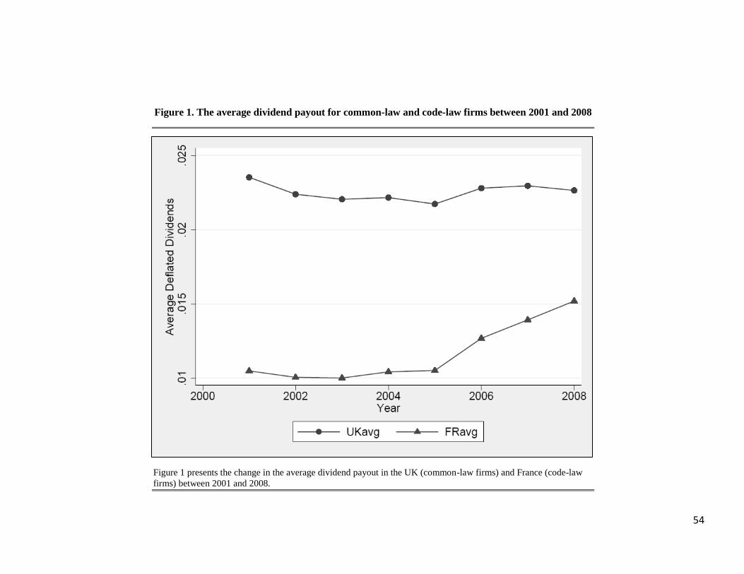
54
Figure 1. The average dividend payout for common-law and code-law firms between 2001 and 2008
Figure 1 presents the change in the average dividend payout in the UK (common-law firms) and France (code-law
firms) between 2001 and 2008.

55
Table 1. Summary statistics of the dividend payout model variables
Full Sample Common-law Sample Code-law Sample
N Mean S.D. Median
N Mean S.D. Median
N Mean S.D. Median
DIVDUM 7415 0.7099 0.4538 1.0000
4340 0.7484 0.4340 1.0000
3075 0.6556 0.4752 1.0000
TDVD 7415 0.0180 0.0206 0.0123
4340 0.0225 0.0221 0.0182
3075 0.0117 0.0162 0.0071
EBI 7415 0.0213 0.1669 0.0520
4340 0.0192 0.1917 0.0582
3075 0.0241 0.1236 0.0458
NI 7415 0.0333 0.5338 0.0970
4340 0.0354 0.5398 0.1008
3075 0.0305 0.5253 0.0932
TAX 7415 0.0188 0.0249 0.0161
4340 0.0191 0.0261 0.0165
3075 0.0184 0.0231 0.0157
RND 7415 0.0208 0.0530 0.0000
4340 0.0236 0.0568 0.0000
3075 0.0168 0.0469 0.0000
TOBINQ 7415 1.0543 1.1176 0.7151
4340 1.1922 1.1945 0.8159
3075 0.8597 0.9662 0.5780
%∆TA 7415 0.1285 0.4512 0.0491
4340 0.1472 0.4919 0.0574
3075 0.1019 0.3852 0.0430
LOGTA 7415 12.4348 2.0837 12.1373
4340 12.2907 2.0098 12.0579
3075 12.6382 2.1678 12.2677
LEV 7415 0.5788 0.2341 0.5855
4340 0.5454 0.2387 0.5479
3075 0.6261 0.2189 0.6301
REPUR 7415 0.0383 0.2557 0.0000
4340 0.0591 0.3325 0.0000
3075 0.0089 0.0161 0.0021
LOSS 7415 0.2384 0.4262 0.0000
4340 0.2482 0.4320 0.0000
3075 0.2247 0.4175 0.0000
TANG 7415 0.2407 0.2176 0.1750
4340 0.2778 0.2421 0.2045
3075 0.1884 0.1635 0.1482
LIQDT 7415 0.0956 0.1225 0.0545 4340 0.1146 0.1442 0.0620 3075 0.0688 0.0748 0.0488
Table 1 reports summary statistics for the variables of the dividend payout model. All variables are defined in Appendix A. All continuous variables are
winsorized at the 1% level to mitigate the influence of outliers.
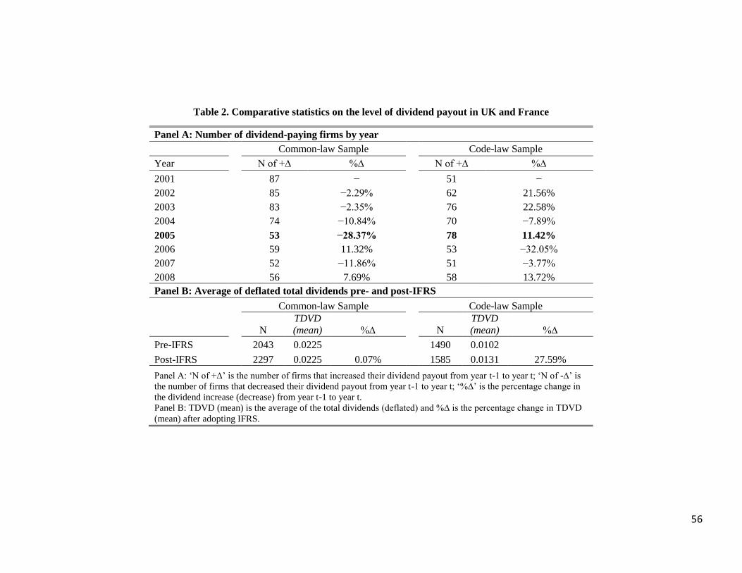
56
Table 2. Comparative statistics on the level of dividend payout in UK and France
Panel A: Number of dividend-paying firms by year
Common-law Sample Code-law Sample
Year
N of +∆ %∆
N of +∆ %∆
2001
87 −
51 −
2002
85 −2.29%
62 21.56%
2003
83 −2.35%
76 22.58%
2004
74 −10.84%
70 −7.89%
2005
53 −28.37%
78 11.42%
2006
59 11.32%
53 −32.05%
2007
52 −11.86%
51 −3.77%
2008
56 7.69% 58 13.72%
Panel B: Average of deflated total dividends pre- and post-IFRS
Common-law Sample Code-law Sample
N
TDVD
(mean) %∆
N
TDVD
(mean) %∆
Pre-IFRS
2043 0.0225
1490 0.0102
Post-IFRS 2297 0.0225 0.07% 1585 0.0131 27.59%
Panel A: ‘N of +∆’ is the number of firms that increased their dividend payout from year t-1 to year t; ‘N of -∆’ is
the number of firms that decreased their dividend payout from year t-1 to year t; ‘%∆’ is the percentage change in
the dividend increase (decrease) from year t-1 to year t.
Panel B: TDVD (mean) is the average of the total dividends (deflated) and %∆ is the percentage change in TDVD
(mean) after adopting IFRS.

57
Table 3. Summary statistics of the dividend value relevance model variables
Common-law Sample Code-law Sample
N Mean S.D. Median
N Mean S.D. Median
MV
3688 1.1279 1.0482 0.8056
2373 0.8161 0.8144 0.5862
BVE
3688 0.4501 0.2399 0.4486
2373 0.3793 0.2173 0.3754
NIBX
3688 0.0054 0.1986 0.0422
2373 0.0150 0.1149 0.0329
LOSS
3688 0.2402 0.4273 0.0000
2373 0.2099 0.4073 0.0000
LOSS*BVE
3688 0.1128 0.2510 0.0000
2373 0.0596 0.1728 0.0000
LOSS*NIBX
3688 −0.0485 0.1768 0.0000
2373 −0.0267 0.0953 0.0000
CAPX
3688 0.0479 0.0481 0.0344
2373 0.0453 0.0429 0.0351
∆SALES
3688 0.0571 0.2491 0.0525
2373 0.0458 0.2017 0.0443
LIQDT
3688 0.1127 0.1388 0.0630
2373 0.0715 0.0772 0.0505
∆LTD
3688 0.0103 0.0810 0.0000
2373 0.0041 0.0721 −0.0008
RND
3688 0.0240 0.0579 0.0000
2373 0.0191 0.0497 0.0000
PROCD
3688 0.0263 0.0949 0.0011
2373 0.0154 0.0581 0.0002
TDVD
3688 0.0228 0.0223 0.0186
2373 0.0123 0.0168 0.0075
REPUR
3688 0.0701 0.3618 0.0000
2373 0.0095 0.0175 0.0023
POST
3688 0.5925 0.4914 1.0000
2373 0.6018 0.4896 1.0000
POST*BVE
3688 0.2612 0.2859 0.2254
2373 0.2347 0.2507 0.2249
POST*NIBX
3688 0.0106 0.1341 0.0000
2373 0.0166 0.0726 0.0000
POST*LOSS
3688 0.1261 0.3320 0.0000
2373 0.1066 0.3087 0.0000
POST*LOSS*BVE
3688 0.0587 0.1913 0.0000
2373 0.0313 0.1285 0.0000
POST*LOSS*NIBX
3688 −0.0238 0.1168 0.0000
2373 −0.0111 0.0538 0.0000
(continued on next page)

58
Table 3. (continued)
Common-law Sample Code-law Sample
N Mean S.D. Median N Mean S.D. Median
POST*TDVD
3688 0.0136 0.0209 0.0000
2373 0.0081 0.0157 0.0000
POST*REPUR
3688 0.0699 0.3619 0.0000
2373 0.0068 0.0171 0.0000
OINFO 3688 0.0139 1.0305 −0.0902 2373 −0.0014 0.7768 −0.0902
Table 3 reports summary statistics for the variables of the dividend value relevance model. All variables are defined in Appendix A. All continuous variables are
winsorized at the 1% level to mitigate the influence of outliers.

59
Table 4. Correlation matrix of the dividend payout model for the full sample
(1) (2) (3) (4) (5) (6) (7) (8) (9) (10) (11) (12) (13) (14)
(1) DIVDUM 1.000
(2) TDVD 0.561* 1.000
(3) EBI 0.354* 0.297
* 1.000
(4) NI 0.212* 0.184
* 0.491
* 1.000
(5) TAX 0.375* 0.492
* 0.420
* 0.277
* 1.000
(6) RND −0.269* −0.107
* −0.314
* −0.171
* −0.194
* 1.000
(7) TOBINQ −0.098* 0.249
* −0.128
* −0.031
* 0.194
* 0.376
* 1.000
(8) %∆TA −0.013 −0.078* 0.166
* 0.111
* 0.051
* −0.058
* 0.005 1.000
(9) LOGTA 0.393* 0.137
* 0.236
* 0.132
* 0.141
* −0.223
* −0.194
* 0.014 1.000
(10) LEV 0.026* −0.062
* −0.063
* 0.023
* −0.097
* −0.171
* −0.226
* −0.078
* 0.235
* 1.000
(11) REPUR 0.070* 0.112
* 0.054
* 0.029
* 0.085
* −0.005 0.041
* 0.020 0.109
* 0.024
* 1.000
(12) LOSS −0.431* −0.281
* −0.586
* −0.393
* −0.441
* 0.233
* 0.049
* −0.130
* −0.257
* 0.031
* −0.052
* 1.000
(13) TANG 0.144* 0.113
* 0.116
* 0.055
* 0.019
−0.195
* −0.159
* −0.034
* 0.204
* −0.001 0.022 −0.087
* 1.000
(14) LIQDT −0.199* 0.009 −0.138
* −0.048
* −0.014 0.261
* 0.303
* 0.038
* −0.279
* −0.244
* −0.002 0.117
* −0.256
* 1.000
Table 4 reports the Pearson correlation coefficients between all the variables of the dividend payout model based on the full sample. All variables are defined in Appendix
A. All continuous variables are winsorized at the 1% level to mitigate the influence of outliers. * Denotes significance at the 5% level or better.
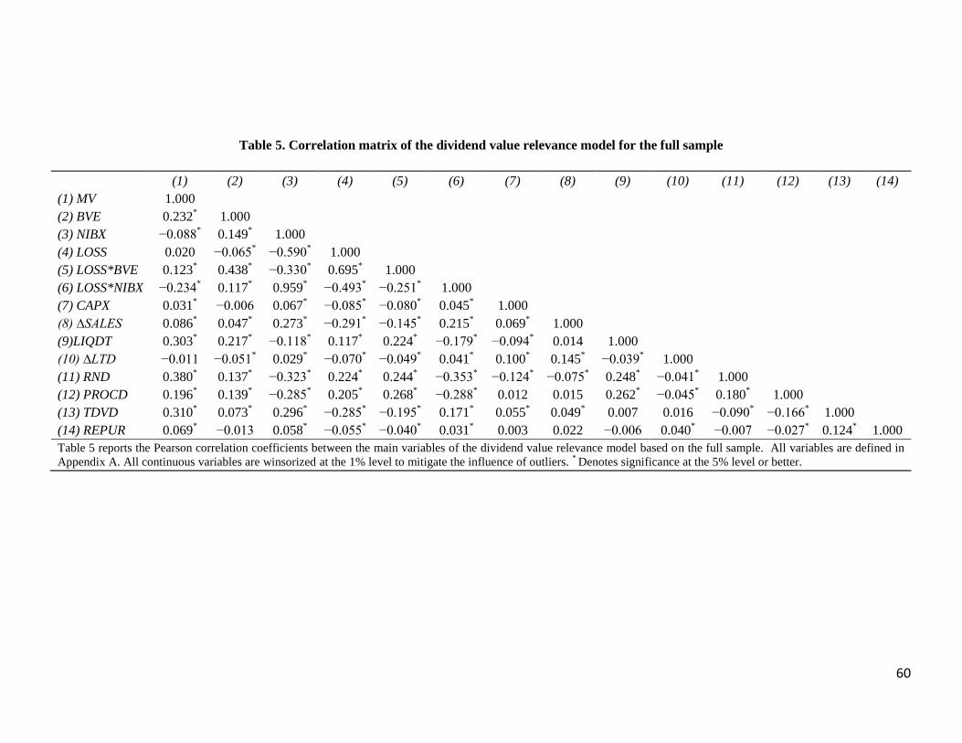
60
Table 5. Correlation matrix of the dividend value relevance model for the full sample
(1) (2) (3) (4) (5) (6) (7) (8) (9) (10) (11) (12) (13) (14)
(1) MV 1.000
(2) BVE 0.232* 1.000
(3) NIBX −0.088* 0.149
* 1.000
(4) LOSS 0.020 −0.065* −0.590
* 1.000
(5) LOSS*BVE 0.123* 0.438
* −0.330
* 0.695
* 1.000
(6) LOSS*NIBX −0.234* 0.117
* 0.959
* −0.493
* −0.251
* 1.000
(7) CAPX 0.031* −0.006 0.067
* −0.085
* −0.080
* 0.045
* 1.000
(8) ∆SALES 0.086* 0.047
* 0.273
* −0.291
* −0.145
* 0.215
* 0.069
* 1.000
(9)LIQDT 0.303* 0.217
* −0.118
* 0.117
* 0.224
* −0.179
* −0.094
* 0.014 1.000
(10) ∆LTD −0.011 −0.051* 0.029
* −0.070
* −0.049
* 0.041
* 0.100
* 0.145
* −0.039
* 1.000
(11) RND 0.380* 0.137
* −0.323
* 0.224
* 0.244
* −0.353
* −0.124
* −0.075
* 0.248
* −0.041
* 1.000
(12) PROCD 0.196* 0.139
* −0.285
* 0.205
* 0.268
* −0.288
* 0.012 0.015 0.262
* −0.045
* 0.180
* 1.000
(13) TDVD 0.310* 0.073
* 0.296
* −0.285
* −0.195
* 0.171
* 0.055
* 0.049
* 0.007 0.016 −0.090
* −0.166
* 1.000
(14) REPUR 0.069* −0.013 0.058
* −0.055
* −0.040
* 0.031
* 0.003 0.022 −0.006 0.040
* −0.007 −0.027
* 0.124
* 1.000
Table 5 reports the Pearson correlation coefficients between the main variables of the dividend value relevance model based on the full sample. All variables are defined in
Appendix A. All continuous variables are winsorized at the 1% level to mitigate the influence of outliers. * Denotes significance at the 5% level or better.

61
Table 6. The change in dividend payouts following IFRS adoption (H1 - OLS regressions)
Common-law Code-law All
TDVD TDVD TDVD
POST −0.0001 0.0019***
−0.0001
(−0.17) (5.29) (−0.12)
CODE −0.0108***
(−12.49)
POST*CODE 0.0021***
(4.15)
EBI 0.0162***
0.0154***
0.0165***
(6.56) (5.77) (8.65)
NI −0.0005 0.0005 −0.0001
(−0.75) (1.24) (−0.33)
TAX 0.3178***
0.2589***
0.3000***
(19.16) (14.54) (24.53)
RND −0.0001 −0.0238***
−0.0102**
(−0.01) (−3.60) (−2.07)
TOBINQ 0.0042***
0.0034***
0.0041***
(10.60) (6.67) (13.29)
%∆TA −0.0064***
−0.0038***
−0.0058***
(−9.36) (−5.38) (−11.17)
LOGTA 0.0006***
0.0005***
0.0007***
(3.84) (4.55) (6.38)
LEV 0.0034**
−0.0073***
0.0007
(2.41) (−5.05) (0.67)
REPUR 0.0030***
0.0322 0.0032***
(3.44) (1.36) (3.68)
LOSS −0.0014* 0.0004 −0.0011
*
(−1.73) (0.53) (−1.90)
TANG 0.0039***
0.0001 0.0029***
(3.10) (0.04) (2.82)
(continued on next page)
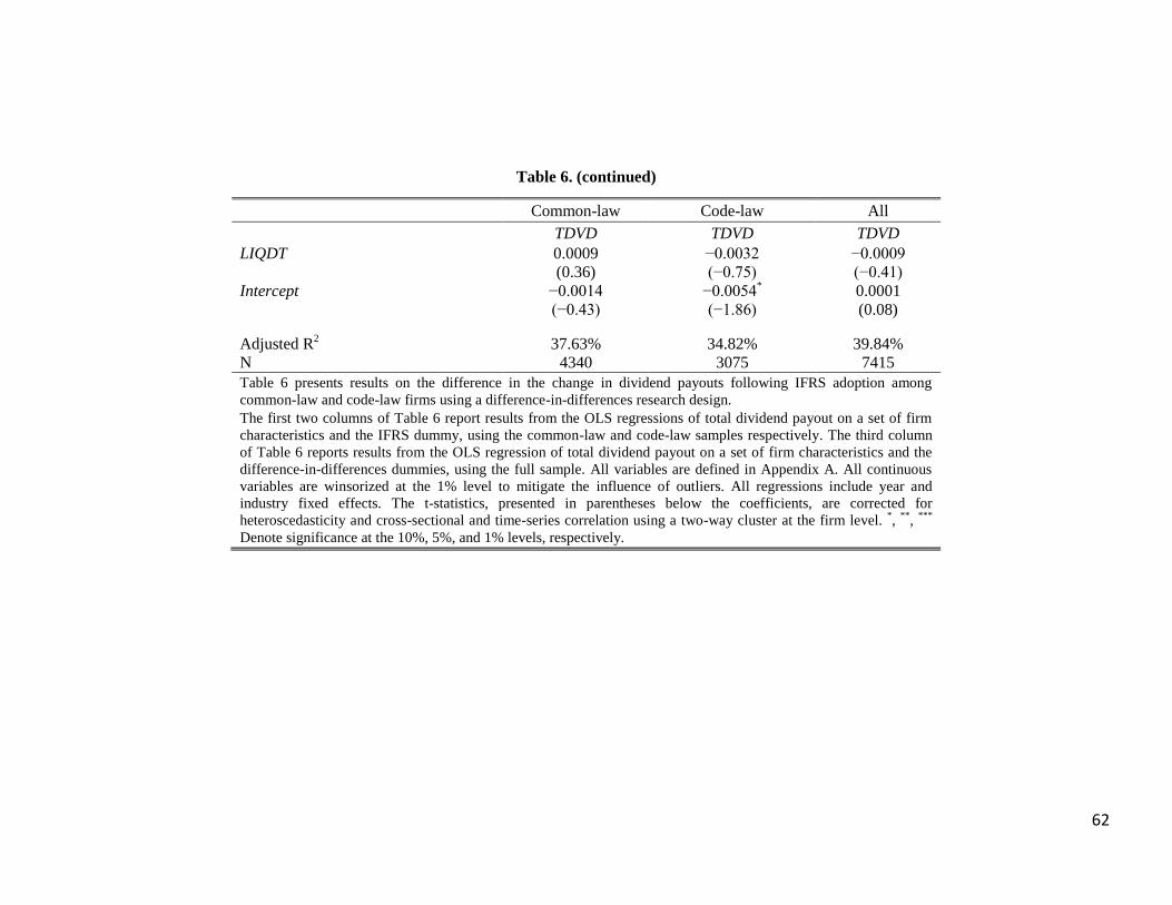
62
Table 6. (continued)
Common-law Code-law All
TDVD TDVD TDVD
LIQDT 0.0009 −0.0032 −0.0009
(0.36) (−0.75) (−0.41)
Intercept −0.0014 −0.0054* 0.0001
(−0.43) (−1.86) (0.08)
Adjusted R2 37.63% 34.82% 39.84%
N 4340 3075 7415
Table 6 presents results on the difference in the change in dividend payouts following IFRS adoption among
common-law and code-law firms using a difference-in-differences research design.
The first two columns of Table 6 report results from the OLS regressions of total dividend payout on a set of firm
characteristics and the IFRS dummy, using the common-law and code-law samples respectively. The third column
of Table 6 reports results from the OLS regression of total dividend payout on a set of firm characteristics and the
difference-in-differences dummies, using the full sample. All variables are defined in Appendix A. All continuous
variables are winsorized at the 1% level to mitigate the influence of outliers. All regressions include year and
industry fixed effects. The t-statistics, presented in parentheses below the coefficients, are corrected for
heteroscedasticity and cross-sectional and time-series correlation using a two-way cluster at the firm level. *,
**,
***
Denote significance at the 10%, 5%, and 1% levels, respectively.

63
Table 7. The change in dividend payouts following IFRS adoption (H1 - Fully Interacted Linear Model)
Common-law Code-law All
TDVD TDVD TDVD
POST 0.0001 0.0019***
0.0001
(0.31) (5.42) (0.21)
CODE −0.0105***
(−12.18)
POST*CODE 0.0020***
(3.97)
EBI 0.0124***
0.0106***
0.0124***
(4.41) (4.06) (4.40)
NI −0.0013 −0.0002 −0.0014
(−1.32) (−0.45) (−1.34)
TAX 0.3632***
0.2332***
0.3649***
(15.58) (11.04) (15.67)
RND −0.0132 −0.0182**
−0.0129
(−1.61) (−2.06) (−1.59)
TOBINQ 0.0028***
0.0024***
0.0029***
(5.71) (4.49) (5.86)
%∆TA −0.0091***
−0.0030***
−0.0090***
(−8.06) (−3.59) (−8.05)
LOGTA 0.0001 0.0003**
0.0001
(0.10) (2.11) (0.82)
LEV 0.0090***
−0.0078***
0.0091***
(4.31) (−5.55) (4.39)
REPUR −0.0317 0.0946***
−0.0426
(−0.28) (2.61) (−0.38)
LOSS −0.0031***
−0.0016* −0.0030
***
(−2.82) (−1.93) (−2.69)
TANG 0.0066***
0.0051***
0.0068***
(4.04) (3.09) (4.19)
(continued on next page)

64
Table 7. (continued)
Common-law Code-law All
TDVD TDVD TDVD
LIQDT −0.0023 0.0065 −0.0017
(−0.69) (1.31) (−0.53)
Intercept 0.0028 0.0025 0.0046
(0.53) (0.50) (1.22)
Adjusted R2 38.90% 36.30% 41.70%
N 4340 3075 7415
Table 7 presents results on the difference in the change in dividend payouts following IFRS adoption among
common-law and code-law firms using a fully interacted linear model of the difference-in-differences research
design.
The first two columns of Table 7 report results from the OLS regressions of total dividend payout on a set of firm
characteristics and the IFRS dummy, after interacting all variables with the IFRS dummy, using the common-law
and code-law samples respectively. The third column of Table 7 reports results from the OLS regression of total
dividend payout on a set of firm characteristics and the difference-in-differences dummies, after interacting all
variables with the difference-in-differences dummies, using the full sample. We do not report the coefficients on the
interactions for the sake of brevity. All variables are defined in Appendix A. All continuous variables are winsorized
at the 1% level to mitigate the influence of outliers. All regressions include year and industry fixed effects. The t-
statistics, presented in parentheses below the coefficients, are corrected for heteroscedasticity by clustering at the
firm level. *,
**,
*** Denote significance at the 10%, 5%, and 1% levels, respectively.

65
Table 8. The change in dividend payouts following IFRS adoption (H1 - Logistic regressions)
Common-law Code-law All
DIVDUM DIVDUM DIVDUM
POST −0.1050 0.5510***
0.0456
(−0.59) (3.13) (0.30)
CODE −1.3230***
(−7.81)
POST*CODE 0.3500**
(2.24)
EBI 1.5270***
3.5110***
1.5530***
(3.46) (4.03) (3.91)
NI −0.134 0.2040* −0.0057
(−1.00) (1.72) (−0.07)
TAX 24.6701***
34.2609***
28.0540***
(7.17) (8.00) (10.25)
RND −5.5750***
−5.1010***
−4.4030***
(−2.80) (−2.64) (−3.09)
TOBINQ 0.0376 −0.1230 −0.0055
(0.46) (−1.11) (−0.09)
%∆TA −0.5250***
−0.0760 −0.3980***
(−5.22) (−0.60) (−5.08)
LOGTA 0.3740***
0.5110***
0.4600***
(5.99) (8.36) (10.41)
LEV −0.1210 −2.4080***
−0.9470***
(−0.33) (−5.38) (−3.46)
REPUR 0.6110**
15.8800**
0.5830
(2.00) (2.22) (1.67)
LOSS −1.0920***
−0.8660***
−1.0838***
(−7.05) (−4.37) (−9.00)
TANG −0.5430 0.1406 −0.3120
(−1.18) (0.21) (−0.84)
(continued on next page)
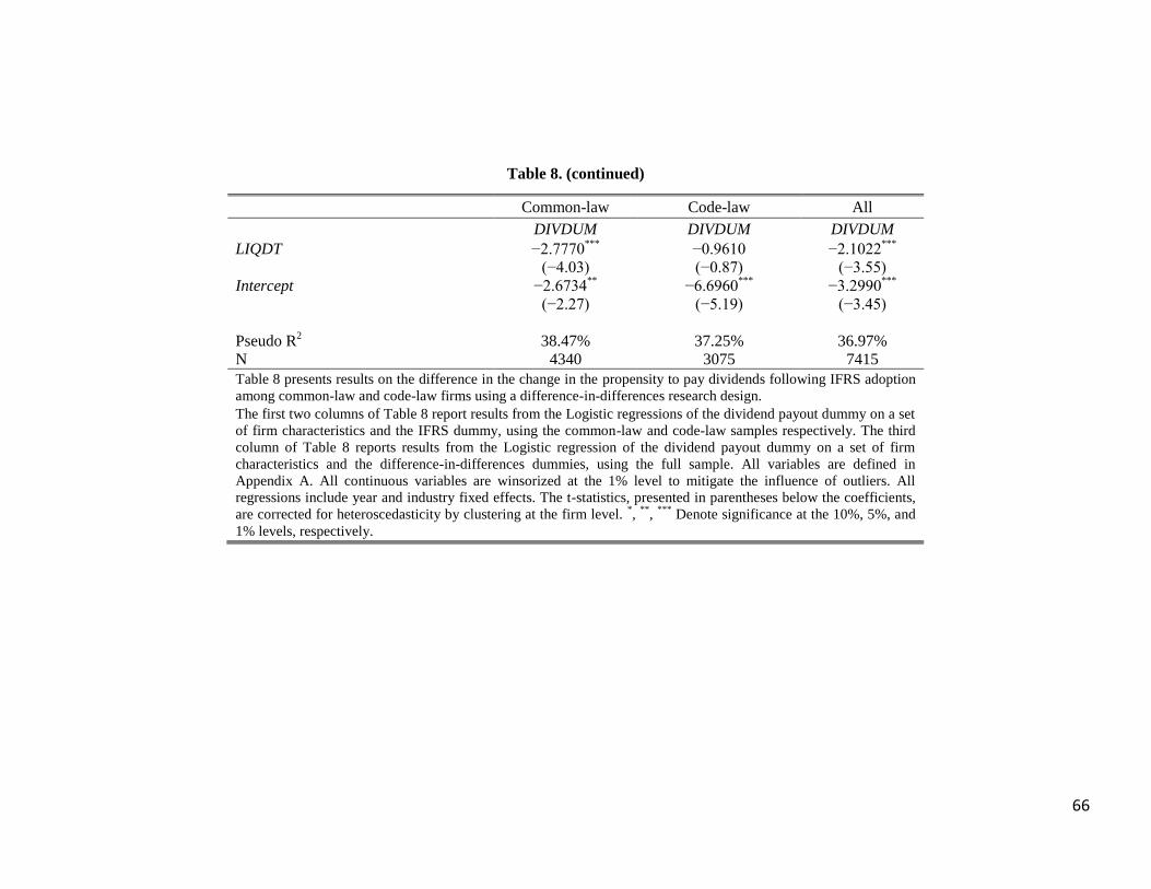
66
Table 8. (continued)
Common-law Code-law All
DIVDUM DIVDUM DIVDUM
LIQDT −2.7770***
−0.9610 −2.1022***
(−4.03) (−0.87) (−3.55)
Intercept −2.6734**
−6.6960***
−3.2990***
(−2.27) (−5.19) (−3.45)
Pseudo R2 38.47% 37.25% 36.97%
N 4340 3075 7415
Table 8 presents results on the difference in the change in the propensity to pay dividends following IFRS adoption
among common-law and code-law firms using a difference-in-differences research design.
The first two columns of Table 8 report results from the Logistic regressions of the dividend payout dummy on a set
of firm characteristics and the IFRS dummy, using the common-law and code-law samples respectively. The third
column of Table 8 reports results from the Logistic regression of the dividend payout dummy on a set of firm
characteristics and the difference-in-differences dummies, using the full sample. All variables are defined in
Appendix A. All continuous variables are winsorized at the 1% level to mitigate the influence of outliers. All
regressions include year and industry fixed effects. The t-statistics, presented in parentheses below the coefficients,
are corrected for heteroscedasticity by clustering at the firm level. *,
**,
*** Denote significance at the 10%, 5%, and
1% levels, respectively.

67
Table 9. The change in dividend payouts following IFRS adoption (H1 - Firm Fixed Effects regressions)
Common-law Code-law All
TDVD TDVD TDVD
POST 0.0008 0.0016***
0.0005
(1.41) (3.29) (0.99)
CODE
POST*CODE 0.0016**
(2.22)
EBI 0.0011 0.0032 0.0012
(0.48) (1.31) (0.67)
NI −0.0008 0.0001 −0.0003
(−1.61) (0.93) (−1.31)
TAX 0.0855***
0.0563**
0.0746***
(5.11) (2.57) (5.74)
RND −0.0007 0.0024 −0.0007
(−0.07) (0.25) (−0.12)
TOBINQ 0.0014***
0.0025***
0.0018***
(3.71) (4.18) (5.61)
%∆TA −0.0025***
−0.0026***
−0.0025***
(−5.71) (−4.66) (−7.31)
LOGTA 0.0002 0.0018 0.0008
(0.27) (1.87) (1.37)
LEV −0.0047* −0.0028 −0.0043
**
(−1.75) (−1.22) (−2.25)
REPUR 0.0020***
0.0494**
0.0021***
(2.66) (2.03) (2.71)
LOSS −0.0007 0.0001 −0.0004
(−1.02) (0.21) (−0.78)
TANG 0.0048 −0.0001 0.0035
(1.38) (−0.04) (1.30)
(continued on next page)

68
Table 9. (continued)
Common-law Code-law All
TDVD TDVD TDVD
LIQDT 0.0018 0.0022 0.0018
(0.65) (0.41) (0.75)
Intercept 0.0177* −0.0140 0.0051
(1.83) (−1.08) (0.65)
Overall R2 22.37% 19.64% 23.20%
N 4340 3075 7415
Table 9 presents results on the difference in the change in dividend payouts following IFRS adoption among
common-law and code-law firms using a difference-in-differences research design
The first two columns of Table 9 report results from the firm Fixed Effects regressions of total dividend payout on a
set of firm characteristics and the IFRS dummy, using the common-law and code-law samples respectively. The
third column of Table 9 reports results from the firm Fixed Effect regression of total dividend payout on a set of firm
characteristics and the difference-in-differences dummies, using the full sample. All variables are defined in
Appendix A. All continuous variables are winsorized at the 1% level to mitigate the influence of outliers. All
regressions include year fixed effects. The t-statistics, presented in parentheses below the coefficients, are corrected
for heteroscedasticity by clustering at the firm level. *,
**,
*** Denote significance at the 10%, 5%, and 1% levels,
respectively.
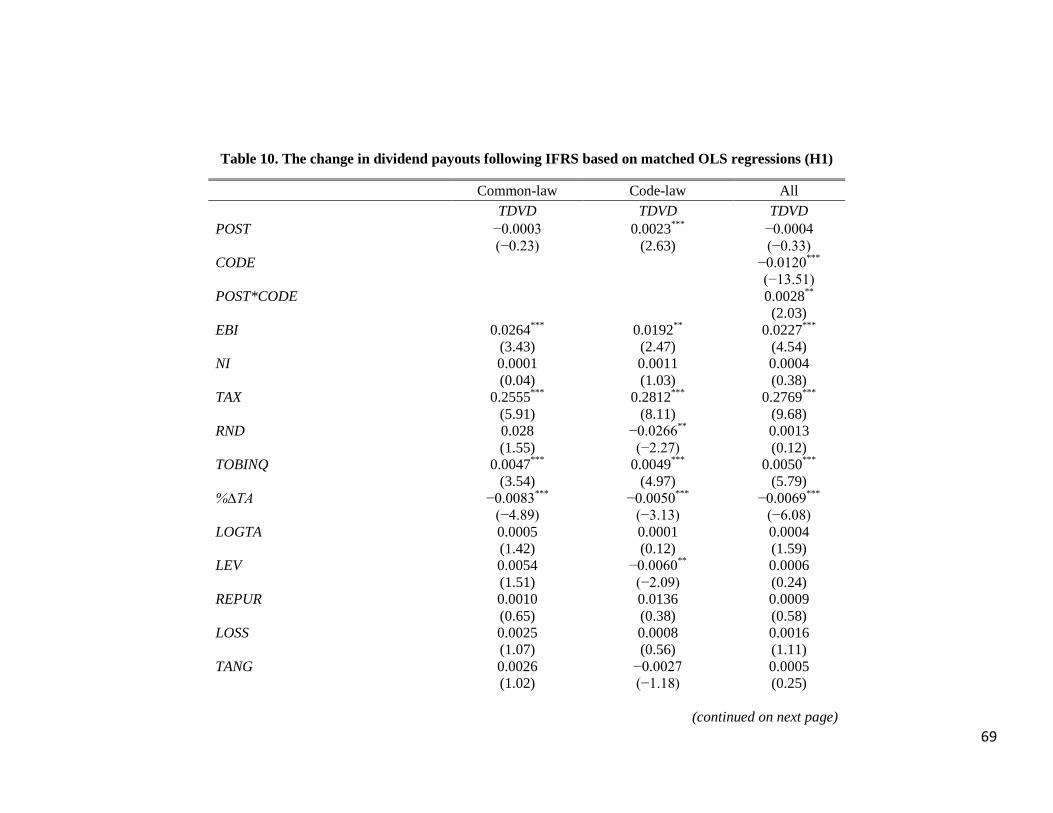
69
Table 10. The change in dividend payouts following IFRS based on matched OLS regressions (H1)
Common-law Code-law All
TDVD TDVD TDVD
POST −0.0003 0.0023***
−0.0004
(−0.23) (2.63) (−0.33)
CODE −0.0120***
(−13.51)
POST*CODE 0.0028**
(2.03)
EBI 0.0264***
0.0192**
0.0227***
(3.43) (2.47) (4.54)
NI 0.0001 0.0011 0.0004
(0.04) (1.03) (0.38)
TAX 0.2555***
0.2812***
0.2769***
(5.91) (8.11) (9.68)
RND 0.028 −0.0266**
0.0013
(1.55) (−2.27) (0.12)
TOBINQ 0.0047***
0.0049***
0.0050***
(3.54) (4.97) (5.79)
%∆TA −0.0083***
−0.0050***
−0.0069***
(−4.89) (−3.13) (−6.08)
LOGTA 0.0005 0.0001 0.0004
(1.42) (0.12) (1.59)
LEV 0.0054 −0.0060**
0.0006
(1.51) (−2.09) (0.24)
REPUR 0.0010 0.0136 0.0009
(0.65) (0.38) (0.58)
LOSS 0.0025 0.0008 0.0016
(1.07) (0.56) (1.11)
TANG 0.0026 −0.0027 0.0005
(1.02) (−1.18) (0.25)
(continued on next page)

70
Table 10. (continued)
Common-law Code-law All
TDVD TDVD TDVD
LIQDT −0.0037 −0.0146**
−0.0070
(−0.55) (−1.99) (−1.32)
Intercept −0.0018 0.0073 −0.0181***
(−0.24) (1.11) (−4.99)
Adjusted R2 23.82% 38.19% 33.10%
N 1024 1024 2048
Table 10 presents results on the difference in the change in dividend payouts following IFRS adoption among
common-law and code-law firms using a matched difference-in-differences research design. The regressions are
matched, using CEM matching, based on ROA, Total Assets, Industry and IFRS. The first two columns of Table 10
report results from the OLS regressions of total dividend payout on a set of firm characteristics and the IFRS
dummy, using the common-law and code-law matched observations respectively. The third column of Table 10
reports results from the OLS regression of total dividend payout on a set of firm characteristics and the difference-
in-differences dummies, using the full matched sample. All variables are defined in Appendix A. All continuous
variables are winsorized at the 1% level to mitigate the influence of outliers. All regressions include year and
industry fixed effects. The t-statistics, presented in parentheses below the coefficients, are corrected for
heteroscedasticity by clustering at the firm level. *,
**,
*** Denote significance at the 10%, 5%, and 1% levels,
respectively.

71
Table 11. The variation in the IFRS effect on dividend payouts among code-law firms (H2 - ACCDUM1)
High Quality Low Quality All
TDVD TDVD TDVD
POST 0.0016**
0.0030***
0.0014*
(2.14) (4.79) (1.90)
ACCDUM1 −0.0002
(−0.25)
POST*ACCDUM1 0.0022**
(2.27)
EBI 0.0103***
0.0310***
0.0157***
(4.28) (3.41) (5.93)
NI 0.0003 0.0016 0.0005
(0.71) (1.63) (1.30)
TAX 0.2321***
0.2100***
0.2565***
(9.31) (8.38) (14.38)
RND −0.0234***
−0.0285***
−0.0241***
(−2.87) (−3.20) (−3.66)
TOBINQ 0.0017***
0.0066***
0.0034***
(3.09) (8.48) (6.76)
%∆TA −0.0032***
−0.0041***
−0.0037***
(−4.14) (−3.30) (−5.27)
LOGTA 0.0007***
0.0004***
0.0005***
(3.06) (2.75) (3.65)
LEV −0.0062***
−0.0116***
−0.0071***
(−4.55) (−4.28) (−4.86)
REPUR −0.0006 0.0775***
0.0325
(−0.02) (2.88) (1.39)
(continued on next page)

72
Table 11. (continued)
High Quality Low Quality All
TDVD TDVD TDVD
LOSS −0.0009 0.0017 0.0004
(−0.95) (1.54) (0.51)
TANG 0.0025 −0.003 −0.0005
(0.81) (−1.41) (−0.26)
LIQDT 0.007 −0.0142**
−0.0032
(1.26) (−2.04) (−0.74)
Intercept 0.0014 0.0130***
0.005
(0.20) (3.61) (1.51)
Adjusted R2 29.51% 44.22% 35.00%
N 1511 1564 3075
Table 11 presents results on the difference in the change in dividend payouts following IFRS adoption among high-
and low- accounting quality firms in the code-law sample using a difference-in-differences research design. In this
table we use the average absolute value of discretionary accruals, in years prior to IFRS, after controlling for
idiosyncratic economic shocks, as a proxy for accounting quality.
The first two columns of Table 11 report results from the OLS regressions of total dividend payout on a set of firm
characteristics and the IFRS dummy, using the high- and low- accounting quality firms in the code-law samples
respectively. The third column of Table 11 reports results from the OLS regression of total dividend payout on a set
of firm characteristics and the difference-in-differences dummies, using all code-law firms. The average of absolute
value of discretionary accruals is the used criterion in categorizing code-law firms as high- or low- accounting
quality firms. All variables are defined in Appendix A. All continuous variables are winsorized at the 1% level to
mitigate the influence of outliers. All regressions include year and industry fixed effects. The t-statistics, presented
in parentheses below the coefficients, are corrected for heteroscedasticity by clustering at the firm level. *,
**,
***
Denote significance at the 10%, 5%, and 1% levels, respectively.

73
Table 12. The variation in the IFRS effect on dividend payouts among code-law firms (H2 - ACCDUM2)
High Quality Low Quality All
TDVD TDVD TDVD
POST 0.0009 0.0035***
0.0009
(1.26) (5.23) (1.39)
ACCDUM2 0.0008
(1.32)
POST*ACCDUM2 0.0032***
(3.35)
EBI 0.0099***
0.0326***
0.0157***
(4.32) (2.75) (5.97)
NI 0.0001 0.0045**
0.0005
(0.40) (1.99) (1.25)
TAX 0.2244***
0.2047***
0.2549***
(9.71) (7.17) (14.39)
RND −0.0137* −0.0486
*** −0.0244
***
(−1.75) (−4.59) (−3.72)
TOBINQ 0.0017***
0.0078***
0.0035***
(3.28) (6.82) (6.90)
%∆TA −0.0026***
−0.0046***
−0.0035***
(−3.86) (−3.60) (−5.04)
LOGTA 0.0008***
0.0001 0.0004***
(4.58) (0.43) (3.19)
LEV −0.0047***
−0.0109***
−0.0067***
(−3.84) (−3.53) (−4.73)
REPUR 0.0288 0.1021***
0.0355
(1.19) (2.98) (1.51)
(continued on next page)

74
Table 12. (continued)
High Quality Low Quality All
TDVD TDVD TDVD
LOSS −0.0007 0.0023* 0.0007
(−0.92) (1.72) (0.99)
TANG −0.002 0.0003 −0.0009
(−1.07) (0.11) (−0.53)
LIQDT −0.0012 −0.0116 −0.0036
(−0.26) (−1.57) (−0.84)
Intercept −0.0011 0.0033 0.0053
(−0.27) (0.79) (1.63)
Adjusted R2 30.97% 45.34% 35.51%
N 1592 1483 3075
Table 12 presents results on the difference in the change in dividend payouts following IFRS adoption among high-
and low- accounting quality firms in the code-law sample using a difference-in-differences research design. In this
table we use the variance of the firm’s discretionary accruals in years prior to IFRS, calculated following Dechow
and Dichev (2002), as a proxy for accounting quality.
The first two columns of Table 12 report results from the OLS regressions of total dividend payout on a set of firm
characteristics and the IFRS dummy, using the high- and low- accounting quality firms in the code-law samples
respectively. The third column of Table 12 reports results from the OLS regression of total dividend payout on a set
of firm characteristics and the difference-in-differences dummies, using all code-law firms. The variance of
discretionary accruals is the used criterion in categorizing code-law firms as high- or low- accounting quality firms.
All variables are defined in Appendix A. All continuous variables are winsorized at the 1% level to mitigate the
influence of outliers. All regressions include year and industry fixed effects. The t-statistics, presented in
parentheses below the coefficients, are corrected for heteroscedasticity by clustering at the firm level. *,
**,
***
Denote significance at the 10%, 5%, and 1% levels, respectively.
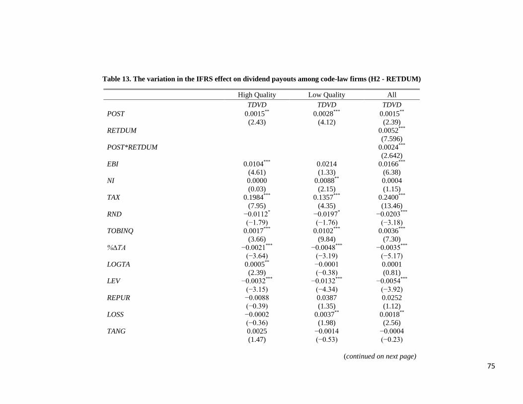
75
Table 13. The variation in the IFRS effect on dividend payouts among code-law firms (H2 - RETDUM)
High Quality Low Quality All
TDVD TDVD TDVD
POST 0.0015**
0.0028***
0.0015**
(2.43) (4.12) (2.39)
RETDUM 0.0052***
(7.596)
POST*RETDUM 0.0024***
(2.642)
EBI 0.0104***
0.0214 0.0166***
(4.61) (1.33) (6.38)
NI 0.0000 0.0088**
0.0004
(0.03) (2.15) (1.15)
TAX 0.1984***
0.1357***
0.2400***
(7.95) (4.35) (13.46)
RND −0.0112* −0.0197
* −0.0203
***
(−1.79) (−1.76) (−3.18)
TOBINQ 0.0017***
0.0102***
0.0036***
(3.66) (9.84) (7.30)
%∆TA −0.0021***
−0.0048***
−0.0035***
(−3.64) (−3.19) (−5.17)
LOGTA 0.0005**
−0.0001 0.0001
(2.39) (−0.38) (0.81)
LEV −0.0032***
−0.0132***
−0.0054***
(−3.15) (−4.34) (−3.92)
REPUR −0.0088 0.0387 0.0252
(−0.39) (1.35) (1.12)
LOSS −0.0002 0.0037**
0.0018**
(−0.36) (1.98) (2.56)
TANG 0.0025 −0.0014 −0.0004
(1.47) (−0.53) (−0.23)
(continued on next page)

76
Table 13. (continued)
High Quality Low Quality All
TDVD TDVD TDVD
LIQDT 0.0053 −0.0031 −0.0004
(1.02) (−0.41) (−0.10)
Intercept −0.0080**
0.0170***
0.0080***
(−2.00) (3.39) (2.57)
Adjusted R2 25.35% 42.61% 37.44%
N 1483 1592 3075
Table 13 presents results on the difference in the change in dividend payouts following IFRS adoption among high-
and low- accounting quality firms in the code-law sample using a difference-in-differences research design. In this
table we use the firm’s average annualized variance of stock returns, in years prior to IFRS, as a proxy for
accounting quality.
The first two columns of Table 13 report results from the OLS regressions of total dividend payout on a set of firm
characteristics and the IFRS dummy, using the high- and low- accounting quality firms in the code-law samples
respectively. The third column of Table 13 reports results from the OLS regression of total dividend payout on a set
of firm characteristics and the difference-in-differences dummies, using all code-law firms. The average of the
annualized variance of daily stock returns is the used criterion in categorizing code-law firms as high- or low-
accounting quality firms. All variables are defined in Appendix A. All continuous variables are winsorized at the 1%
level to mitigate the influence of outliers. All regressions include year and industry fixed effects. The t-statistics,
presented in parentheses below the coefficients, are corrected for heteroscedasticity by clustering at the firm level. *,
**,
*** Denote significance at the 10%, 5%, and 1% levels, respectively.
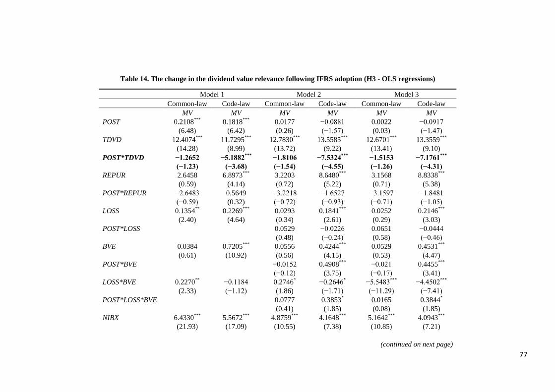
77
Table 14. The change in the dividend value relevance following IFRS adoption (H3 - OLS regressions)
Model 1 Model 2 Model 3
Common-law Code-law Common-law Code-law Common-law Code-law
MV MV MV MV MV MV
POST 0.2108***
0.1818***
0.0177 −0.0881 0.0022 −0.0917
(6.48) (6.42) (0.26) (−1.57) (0.03) (−1.47)
TDVD 12.4074***
11.7295***
12.7830***
13.5585***
12.6701***
13.3559***
(14.28) (8.99) (13.72) (9.22) (13.41) (9.10)
POST*TDVD −1.2652 −5.1882***
−1.8106 −7.5324***
−1.5153 −7.1761***
(−1.23) (−3.68) (−1.54) (−4.55) (−1.26) (−4.31)
REPUR 2.6458 6.8973***
3.2203 8.6480***
3.1568 8.8338***
(0.59) (4.14) (0.72) (5.22) (0.71) (5.38)
POST*REPUR −2.6483 0.5649 −3.2218 −1.6527 −3.1597 −1.8481
(−0.59) (0.32) (−0.72) (−0.93) (−0.71) (−1.05)
LOSS 0.1354**
0.2269***
0.0293 0.1841***
0.0252 0.2146***
(2.40) (4.64) (0.34) (2.61) (0.29) (3.03)
POST*LOSS 0.0529 −0.0226 0.0651 −0.0444
(0.48) (−0.24) (0.58) (−0.46)
BVE 0.0384 0.7205***
0.0556 0.4244***
0.0529 0.4531***
(0.61) (10.92) (0.56) (4.15) (0.53) (4.47)
POST*BVE −0.0152 0.4908***
−0.021 0.4455***
(−0.12) (3.75) (−0.17) (3.41)
LOSS*BVE 0.2270**
−0.1184 0.2746* −0.2646
* −5.5483
*** −4.4502
***
(2.33) (−1.12) (1.86) (−1.71) (−11.29) (−7.41)
POST*LOSS*BVE 0.0777 0.3853* 0.0165 0.3844
*
(0.41) (1.85) (0.08) (1.85)
NIBX 6.4330***
5.5672***
4.8759***
4.1648***
5.1642***
4.0943***
(21.93) (17.09) (10.55) (7.38) (10.85) (7.21)
(continued on next page)

78
Table 14. (continued)
Model 1 Model 2 Model 3
Common-law Code-law Common-law Common-law Code-law Common-law
MV MV MV MV MV MV
POST*NIBX 2.4280***
1.9504***
1.9957***
2.0793***
(4.28) (2.94) (3.35) (3.07)
LOSS*NIBX −7.3179***
−6.0923***
−5.2069***
−4.2543***
0.3163**
−0.3352**
(−23.89) (−17.00) (−10.99) (−7.17) (2.12) (−2.18)
POST*LOSS*NIBX −3.7861***
−3.3391***
−3.2574***
−3.0550***
(−6.51) (−4.64) (−5.25) (−4.15)
CAPX 1.4516***
0.6239**
1.4482***
0.6452***
1.3239***
0.5262
(5.96) (2.50) (6.03) (2.62) (3.53) (1.33)
POST*CAPX 0.1455 0.1726
(0.31) (0.35)
∆SALES 0.2610***
0.2412***
0.2647***
0.2481***
0.1901***
0.4302***
(5.44) (4.27) (5.58) (4.43) (2.74) (5.31)
POST*∆SALES 0.1338 −0.2957***
(1.41) (−2.67)
LIQDT 0.4527***
0.2547* 0.4167
*** 0.2512
* 0.3833
*** 0.3226
(4.94) (1.82) (4.61) (1.82) (2.91) (1.39)
POST*LIQDT 0.0455 −0.0617
(0.26) (−0.22)
∆LTD −0.1383 0.1770 −0.1077 0.2195 −0.1352 −0.2883
(−0.98) (1.21) (−0.78) (1.52) (−0.59) (−1.27)
POST*∆LTD 0.049 0.8365***
(0.17) (2.88)
RND 5.4741***
3.3614***
5.4418***
3.2082***
4.6215***
2.6889***
(21.84) (14.37) (22.03) (13.85) (13.88) (8.15)
(continued on next page)

79
Table 14. (continued)
Model 1 Model 2 Model 3
Common-law Code-law Common-law Common-law Code-law Common-law
MV MV MV MV MV MV
POST*RND 1.5335***
0.9219**
(3.51) (2.10)
PROCD 1.0700***
−0.1271 0.9173***
−0.1905 1.3032***
−1.2176***
(8.21) (−0.69) (7.06) (−1.03) (6.12) (−3.68)
POST*PROCD −0.5513**
1.4902***
(−2.05) (3.76)
OINFO 0.3567***
0.4401***
0.3602***
0.4537***
0.3587***
0.4679***
(33.57) (32.91) (33.68) (34.06) (33.45) (35.18)
1/TA 2117.4988***
3664.9529***
2133.2240***
3980.1302***
2111.0392***
3939.5557***
(6.24) (8.26) (6.36) (9.06) (6.19) (9.06)
H0:
POST*TDVD (UK) =
POST*TDVD (France)
Chi2 = 2.83
p-value = 0.0925
Chi2 = 4.37
p-value = 0.0360
Chi2 = 4.12
p-value = 0.0424
Adjusted R2 81.43% 82.08% 81.97% 82.65% 81.99% 83.13%
N 3688 2373 3688 2373 3688 2373
Model 1 of Table 14 reports results from the OLS regressions of market value on a set of firm characteristics, the IFRS dummy and
interactions between the IFRS dummy with total dividends and stock repurchases, using common-law and code-law samples. Model
2 of Table 14 reports results from the OLS regressions of market value on a set of firm characteristics, the IFRS dummy, and the
interaction between the IFRS dummy with accounting variables, total dividends and stock repurchases, using the common-law and
code-law samples. Model 3 of Table 14 reports results from the OLS regressions of market value on a set of firm characteristics, the
IFRS dummy and the interaction between the IFRS dummy and all other variables, using the common-law and code-law samples.
We use the Chi2 statistic in order to test the significance of the difference in the change in dividend value relevance between the
common-law and the code-law samples. All variables are defined in Appendix A. All continuous variables are winsorized at the 1%
level to mitigate the influence of outliers. All regressions include year and industry fixed effects. The t-statistics, presented in
parentheses below the coefficients, are corrected for heteroscedasticity by clustering at the firm level. *,
**,
*** Denote significance at
the 10%, 5%, and 1% levels, respectively.
80
Chapter 3
Does Changing Accounting Standards Affect Equity Financing?
ABSTRACT: Prior literature indicates that managers manipulate earnings prior to issuing
Seasoned Equity Offerings (SEOs), especially when information asymmetry is high. We
exploit the mandatory adoption of IFRS in Europe in 2005 in order to test the change in the
level of earnings management prior to issuing SEOs in the UK and France. The UK is a
common-law country with an accounting system similar to IFRS, whereas France is a
code-law country with an accounting system that differs materially from IFRS. Despite this
difference, both countries are highly comparable economically and institutionally. This
facilitates the implementation of a difference-in-differences methodology, where the UK is
the control group and France is the treatment group. Our findings suggest that, following
IFRS adoption, earnings management activities decrease among code-law firms prior to
issuing SEOs. As a result of the lower levels of earnings management and information
asymmetry, we predict and find that the market reaction to issuing SEOs improves
significantly for code-law firms following IFRS. Given that equity financing becomes less
costly, we find that the propensity to issue new SEOs increases among code-law firms after
IFRS adoption. The results persist after running a matched-sample analysis and controlling
for self-selection bias.
Keywords: IFRS; Information Asymmetry; Earnings Management; Seasoned Equity
Offerings; Equity Financing.
81
3.1. Introduction
Since the implementation of International Financial Reporting Standards (IFRS) in 2005 in
the European Union, a large number of studies have examined the consequences of the
mandatory adoption of IFRS. This paper adds to this long standing literature and examines
the effect of IFRS adoption on various aspects of seasoned equity offerings (SEOs).
Specifically, we evaluate the change in the level of earnings management prior to issuing
SEOs, the change in the market reaction to SEO announcements and the change in the
propensity to issue SEOs following the IFRS mandate.
We examine these issues using a difference-in-differences research design, after we
control for potential factors that might confound with IFRS adoption. We differentiate
between common-law and code-law legal systems since accounting standards differ
materially between both systems (La Porta, Lopez-De-Silanes, Shleifer, & Vishny, 1998).
We expect IFRS to have a greater impact in code-law countries due to the material
difference between the code-law accounting standards and IFRS (Hong, Hung, & Lobo,
2014; Joos & Lang, 1994; Kaufmann, Kraay, & Mastruzzi, 2007). Thus, code-law firms
serve as a treatment group for our test of the IFRS adoption effect. On the other hand, we
expect a nominal effect for IFRS adoption in common-law countries because IFRS were
initially developed in the spirit of common-law accounting standards (Ball, Kothari, &
Robin, 2000). As such, common-law firms serve as a control group for testing the impact
of IFRS adoption. We select the UK as a common-law country and France as a code-law
country. This selection is based on the high comparability between both economies, which
leaves the difference in accounting standards prior to mandatory IFRS adoption the main
variant factor (see section 3.5.1 for details). Based on this setting, we formulate the
following three hypotheses.
First, we hypothesize that IFRS adoption will moderate earnings management prior to
issuing SEOs among code-law firms. Warfield, Wild, & Wild (1995) find that the level of
earnings management is higher when information asymmetry is higher. In an SEO setting,
82
Teoh et al. (1998) and Shivakumar (2000) find that managers manipulate earnings prior to
SEO announcements. To the extent IFRS mitigate information asymmetry (Daske, Hail,
Leuz, & Verdi, 2008; Muller, Riedl, & Sellhorn, 2011) and improve accounting quality
(Barth, Landsman, & Lang, 2008), we expect mandatory adoption of IFRS to reduce the
level of earnings management prior to issuing SEOs.
Second, we hypothesize that the market reaction to SEO announcements will become
more favorable among code-law firms following IFRS adoption. Myers & Majluf (1984)
theorize that the main reason behind the high cost associated with equity financing is the
existence of asymmetric information, relating to assets in place, between managers and
investors. Therefore, we argue that if IFRS serve to mitigate information asymmetry
relating to assets in place, then the market should attach a lower discount rate for SEOs
after mandatory IFRS adoption.
Third, we hypothesize that the propensity to issue SEOs will increase after IFRS
adoption among code-law firms. Eckbo, Masulis, & Norli (2007) document that issuing
SEOs is a rare phenomenon among public firms because investors underprice the offered
shares due to the existence of asymmetric information and the adverse selection problem.
If IFRS serve to mitigate information asymmetry and consequently improve the market
reaction to SEO announcements, then the cost of equity financing is reduced and managers
are expected to issue SEOs more frequently.
The empirical findings are consistent with our hypotheses. First, we find that the level
of earnings management, prior to issuing SEOs, decreases after IFRS adoption among
code-law firms compared to common-law firms. This finding holds after controlling for
real earnings management (Cohen & Zarowin, 2010) and idiosyncratic economic shocks
(Owens, Wu, & Zimmerman, 2017). Next, we find that the market reaction to SEO
announcements improves after IFRS adoption among code-law firms compared to their
common-law counterparts. This finding holds after controlling for self-selection bias
(Heckman, 1979). Finally, we find that the propensity to issue SEOs increases after IFRS

83
adoption among French firms compared to UK firms. The consistency of observing IFRS
impact on the treatment group, as opposed to the control group, reduces the likelihood that
our findings are attributed to other unidentified confounding effects.
As a robustness check, we run a matched-sample analysis in order to compare firms that
fall on the common support area of the distribution. We use Coarsened Exact Matching
(Iacus, King, & Porro, 2012), where we match each code-law observation to a common-
law observation based on total assets, industry and IFRS time period. The results hold after
running the matched-sample analysis and our conclusions remain unchanged.
Our findings reconcile with Hong et al. (2014) who find that the market reaction to
IPOs has improved globally following IFRS adoption. Our study contributes further to
Hong et al. (2014) by showing that the effect of IFRS adoption on equity financing is not
only transitory around the first equity offering (IPOs), but also permanent around later
equity offerings (SEOs). Moreover, our sample selection focuses on the high comparability
between the treatment and the control groups, based on economic and institutional factors
which cannot be entirely controlled for in international studies.
We contribute to the literature of financial reporting and corporate finance by showing
how changing accounting standards affects corporate financing through SEOs. The main
findings are that IFRS adoption serves to deter earnings management prior to the issue of
SEOs, to improve the market reaction to SEO announcements and to increase the
propensity to issue SEOs. The main implication from this study is that a better financial
reporting system reduces the frictional costs associated with equity financing.
The remainder of the paper is structured as follows: section 3.2 provides the motivation
and literature review; section 3.3 presents the hypotheses development; section 3.4
discusses the research design; section 3.5 describes the data sample; section 3.6 discusses
the main results along with the robustness checks; and section 3.7 concludes.

84
3.2. Motivation & Literature Review
3.2.1. IFRS and Information Asymmetry in the SEO Setting
Myers & Majluf (1984) theorize that equity financing is costly under information
asymmetry relating to assets in place. Uninformed investors will discount the value of the
offered shares because of high ex-ante uncertainty, which increases under asymmetric
information (Akerlof, 1970). Consistent with the information asymmetry theory, Rock
(1986) states that the issuing firm must offer a higher price discount when the level of
uncertainty relating to the fundamental value of the offered shares is higher. Corwin
(2003), among others, provides evidence suggesting that the market reaction to SEOs
issued by firms with high levels of information asymmetry and uncertainty is more
negative. Therefore, theoretical models and empirical findings agree on the strong
association between information asymmetry (uncertainty) and equity under-pricing.
As mentioned before, the relation between the effect of IFRS adoption on aspects of
SEOs relies on prior findings that IFRS mitigate information asymmetry and improve
accounting quality (Armstrong, Barth, Jagolinzer, & Riedl, 2010; Barth et al., 2008; Daske
et al., 2008; Horton, Serafeim, & Serafeim, 2013). The International Accounting Standards
Board (IASB) claims that IFRS are a set of high quality financial reporting standards that
enable investors to compare financial statements across different countries, in addition to
increasing financial reporting transparency (Tweedie, 2006). Consistent with this claim,
recent studies on the consequences of IFRS adoption provide evidence suggesting a
positive impact on capital markets. Li (2010) finds that the adoption of IFRS in European
countries serves to reduce the cost of capital among adopting firms. Byard, Li, & Yu
(2011) find that analysts’ forecast errors and forecast dispersion have decreased
significantly after the mandatory adoption of IFRS in European countries with robust
enforcement of accounting standards. They conclude that IFRS serve to improve the
corporate financial information environment of the adopting firms. Finally, DeFond, Hu,
Hung, & Li (2011) predict and find that the adoption of a unified set of accounting

85
standards, represented by IFRS, increases financial statement comparability and, hence,
increases cross-border investments in Europe. We believe that the benefits associated with
IFRS adoption are expected to mitigate information asymmetry around SEOs. As a result,
we expect improvements in various aspects of equity financing following IFRS adoption.
3.2.2. Earnings Management around SEOs
The tendencies of poor stock returns and poor earnings performance, subsequent to SEOs,
have induced researchers to suspect that earnings are being managed prior to issuing new
equity (Rangan, 1998; Shivakumar, 2000; Teoh et al., 1998; DuCharme, Malatesta, &
Sefcik, 2004). Rangan (1998) finds that firms who issue SEOs have relatively high
abnormal accruals prior to the issue date. He finds that these abnormal accruals predict
poor stock returns and poor earnings performance in post-SEO years. Teoh et al. (1998)
confirm Rangan's (1998) findings and add evidence suggesting that the long-term stock
underperformance and the predictable earnings decline are more prominent among firms
that manipulate their earnings more aggressively prior to issuing SEOs. Shivakumar (2000)
finds similar results to Rangan (1998) and Teoh et al. (1998), but he reaches a different
conclusion from theirs. In contrast to Rangan (1998) and Teoh et al. (1998), who conclude
that managers manipulate their earnings prior to issuing SEOs in order to mislead
investors, Shivakumar (2000) theorizes that investors react efficiently to manipulated
earnings by undoing the manipulation effect through underpricing the issued SEOs. In
other words, Shivakumar (2000) shows that managers manipulate earnings prior to SEOs
in order to increase the stock price, then investors undo this effect by underpricing the
issued SEOs. Despite the difference in the conclusions of the aforementioned authors, they
all find significant evidence of accruals earnings management activities prior to SEOs.
The link between IFRS adoption and the change in the level of earnings management is
based on the findings that IFRS adoption mitigates information asymmetry (Daske et al.,
2008; Muller et al., 2011) and improves accounting quality (Barth et al., 2008). Warfield et

86
al. (1995) document that the level of earnings management is higher under higher levels of
information asymmetry. If IFRS adoption is expected to increase the level of disclosure
and improve accounting quality (Brüggemann, Hitz, & Sellhorn, 2013), which is expected
to mitigate information asymmetry (Daske et al., 2008), then we anticipate a reduction in
the level of earnings management prior to SEOs.
An alternative method for manipulating earnings, other than accruals earnings
management, is real earnings management (Cohen & Zarowin, 2010), where the latter has
a real economic effect on cash flows. Graham, Harvey, & Rajgopal (2005) survey top
executive managers and find that managers prefer to engage in real earnings management
rather than accruals earnings management. According to the surveyed managers, the reason
for this preference is that accruals earnings management is more scrutinized by auditors
and regulators than real earnings management. Consistently, Cohen & Zarowin (2010) find
that firms engage in both types of earnings management prior to issuing SEOs. Therefore,
it is important to take real earnings management activities into account when testing the
change in accruals earnings management following IFRS adoption.
3.2.3. The Market Reaction and the Propensity to Issue SEOs
The finance literature documents strong evidence showing a negative reaction to issuing
new SEOs (Denis, 1994; Eckbo & Masulis, 1995; Jung, Kim, & Stulz, 1996; Masulis &
Korwar, 1986; Mikkelson & Partch, 1986). These studies attribute this common finding to
the existence of asymmetric information, relating to the firm value, between managers and
investors. Eckbo et al. (2007) document in their security offerings’ survey that only one-
quarter of public firms issue SEOs after their initial public offering. According to the
authors, this rare issuance phenomenon is caused by the adverse selection costs associated
with raising external cash.
Prior studies show that firms with a better financial information environment can raise
equity at a lower cost. McLean, Pontiff, & Watanabe (2009) state that equity issuance is

87
more costly in countries with poor financial reporting incentives. Lee & Masulis (2009)
find robust evidence that firms with poor accounting quality encounter higher floatation
costs, higher underwriting costs, a more negative equity issuance reaction, and a higher
probability of withdrawing SEOs. Moreover, Lang & Lundholm (2000) examine the
market reaction to SEO announcements for high-disclosure versus low-disclosure firms.
Their results suggest that high disclosure firms, who maintain a consistent level of
disclosure, experience a hike in their share prices prior to SEO announcements and a minor
decline on the announcement day, compared to low-disclosure firms. The aforementioned
characteristics about financial reporting incentives, accounting quality and disclosure apply
to code-law countries (La Porta et al., 2000; Lee & Masulis, 2009; Singleton-Green, 2015).
This suggests that an improvement in these characteristics should serve to improve the
market reaction to equity financing.
Moreover, Leone, Rock, & Willenborg (2007) document that underpricing of IPOs
increases with the ex-ante uncertainty about the value of the offered stocks; however,
underpricing of IPOs decreases with greater disclosure and better information
environment. Hong et al. (2014) build on Leone et al. (2007) and conduct an international
study with a sample of 29 countries, where they tackle the effect of mandatory IFRS on the
market reaction to IPOs. They implement a difference-in-differences methodology, where
the treatment group consists of 20 adopting countries while the control group consists of 9
non-adopting countries. Their findings suggest that mandatory IFRS adoption reduces
information asymmetry and, consequently, helps firms raise capital at a lower cost, in
addition to facilitating global equity issuance. Accordingly, we predict that the adoption of
IFRS will enhance financial disclosure and improve accounting quality, which is expected
to mitigate information asymmetry, and consequently improve the market reaction to SEO
announcements (Myers & Majluf, 1984).
Finally, Hovakimian & Hutton (2010) find that firms who enjoy a better market reaction
to the first SEO and a better ex-post stock performance, have a higher probability of

88
issuing another SEO. Similarly, if the market reaction to SEOs improves after IFRS
adoption, which reduces the cost of equity financing, then we would expect the propensity
to issue new equity to increase following IFRS adoption.
3.3. Hypothesis Development
Accounting standards in common-law countries are constructed by independent
professional bodies, like the FASB in the US, in order to meet the information needs of
capital market participants (Soderstrom & Sun, 2007). This is similar to the development
of IFRS (Ball et al., 2000), which aims to provide capital market participants with relevant
information for making economic decisions (Brüggemann et al., 2013; Pope & McLeay,
2011). In contrast, accounting standards in code-law countries are constructed by
governments in order to meet their own demands regarding commercial laws and taxation
(Soderstrom & Sun, 2007). This is the main reason why the code-law accounting system
differs materially from IFRS (Hong et al., 2014; Joos & Lang, 1994; Kaufmann et al.,
2007). In light of the preceding argument, we assume that IFRS adoption in code-law
countries will have a greater impact on aspects of SEOs than in common-law countries
(Hong et al., 2014). Furthermore, we discuss potential confounding factors that might drive
our findings at the end of this section.
We hypothesize that the mandatory adoption of IFRS serves to reduce the level of
earnings management prior to issuing SEOs among code-law firms. As mentioned earlier,
prior studies find that firms manage their earnings upwardly before issuing SEOs (Rangan,
1998; Shivakumar, 2000; Teoh et al., 1998), keeping in mind that earnings management
activities increase under higher levels of asymmetric information (Schipper, 1989;
Warfield et al., 1995). If IFRS mitigate information asymmetry (Daske et al., 2008) and
improve accounting quality (Barth et al., 2008), then we expect IFRS adoption to deter
earnings management prior to issuing SEOs, where managerial incentives to inflate

89
earnings are high (Teoh et al., 1998). As such, we formulate the following testable
hypothesis:
Hypothesis (1):
H1: Following IFRS, there is a greater reduction in the level of earnings management prior
to issuing SEOs among code-law firms than common-law firms.
The information shock caused by IFRS adoption is expected to increase financial
statements informative-ness due to the following: (1) mandated increase in disclosure
volume (Ball, Li, & Shivakumar, 2015), (2) improved timeliness and transparency
(Brüggemann et al., 2013), (3) enhanced financial reporting quality (Barth et al., 2008),
and (4) improved financial statement comparability (DeFond et al., 2011). Hence, the main
relationship between IFRS and SEOs arises from the assumption that IFRS are expected to
mitigate information asymmetry relating to assets in place and, therefore, improve the
market reaction to SEOs (Myers & Majluf, 1984). Based on the preceding arguments, we
establish the hypothesis below:
Hypothesis (2):
H2: Following IFRS, there is a greater improvement in the market reaction to SEO
announcements among code-law firms than common-law firms.
Finally, Eckbo et al. (2007) document that the rarity of SEOs is attributed to the high
costs associated with this kind of corporate financing. Supportive evidence is provided by
Hovakimian & Hutton (2010) who find that firms who receive a better market reaction to
their first SEO are more likely to issue a subsequent SEO. If the market reaction to SEO
announcements improves following IFRS adoption, then the associated cost with equity

90
financing is reduced and, accordingly, we expect managers to issue SEOs more frequently.
Therefore, we construct the following hypothesis:
Hypothesis (3):
H3: Following IFRS, there is a greater increase in the propensity to issue SEOs among
code-law firms than common-law firms.
Nevertheless, in order to ascribe capital benefits to IFRS per se, we have to ensure that
other factors associated with accounting quality did not change at the same time. For
instance, if accounting standards were better enforced after IFRS adoption in France, then
our findings would be driven by better enforcement and not by IFRS implementation
(Christensen, Hail, & Leuz, 2013; Leuz & Wysocki, 2016). Brown, Preiato, & Tarca
(2014) construct an international index for the enforcement of accounting standards in
2002, 2005 and 2008. The index shows that the enforcement of accounting standards in
France did not increase around IFRS, and it is similar to the enforcement in the UK, which
improves the comparability between the control and the treatment groups.19
This suggests
that the improvements in the information environment among code-law firms should not be
attributed to the enforcement factor, but to the improvement in accounting standards.
Another factor that might confound our predictions about the effect of IFRS adoption is the
change in the level of corporate governance. Prior studies find that firms with a better
corporate governance enjoy a better market reaction to SEOs because investors are less
worried about ex-post moral hazards (Kim & Purnanandam, 2014). Fortunately,
Katelouzou & Siems (2015) document that the levels of corporate governance and
investor’s protection in the UK and France are similar and sticky over the time period we
cover (2001-2008).
19
The enforcement index (out of 24) for France shows a score of 19, 19 and 16 in 2002, 2005 and 2008,
respectively. For the UK, the score is 14, 22 and 22 in 2002, 2005 and 2008, respectively.

91
3.4. Research Methodology
We test our hypotheses using a difference-in-differences research design. The common-
law sample (UK firms) serves as the control group and the code-law sample (French firms)
serves as the treatment group. As mentioned earlier, the rationale behind our sample
selection is the high comparability between the treatment and the control groups in various
aspects. The selected countries have similar economic, institutional and political factors.
These factors might confound with the effect of IFRS adoption if they were different
between the treatment and the control groups. The similarity in these factors between the
selected countries is the main advantage of our restricted sample selection over
international studies. We provide a detailed discussion of sample selection in section 3.5.1.
The sample period starts in 2001 and ends in 2008 (Hail, Tahoun, & Wang, 2014).20
We
denote the IFRS adoption period using the dummy variable POST that takes the value 1 if
the year is 2005 or beyond, and 0 otherwise. We differentiate the code-law sample from
the common-law sample using the dummy variable CODE that takes the value 1 if the firm
is listed in France (i.e. treated firm), and 0 otherwise. We identify the difference-in-
differences estimator from the interaction between POST and CODE. The interaction term
POST*CODE takes the value 1 if the firm is listed in the code-law country between 2005
and 2008, and 0 otherwise.
3.4.1. Test of Earnings Management
In order to test the change in earnings management prior to issuing SEOs, we mainly
follow Lobo and Zhou (2010) and Iliev (2008) in developing the earnings management
model as shown in equation (1). The dependent variable DACC is the discretionary
accruals calculated in the most recent financial year prior to issuing an SEO. We calculate
discretionary accruals following the modified cross-sectional Jones (1991) model as
20
As a robustness check, we run the regressions after excluding the observations of year 2008 because it is
the beginning of the global financial crisis. In addition, we run the regressions after excluding the
observations of year 2005 as it is considered a transitionary year with high level of information asymmetry
(Wang & Welker, 2011). Our conclusions remain unchanged when excluding year 2008 and/or year 2005
from the sample period.

92
described in Dechow, Sloan, & Sweeney (1995). The procedure for calculating
discretionary accruals is explained in detail in Appendix B. We deflate the variables by the
average of total assets prior to IFRS.21
Initially, the time period used for this test is 2001
till 2008; however, we exclude year 2005 from this regression because SEOs that were
issued in 2005 had their discretionary accruals in 2004 (i.e. before IFRS). We also exclude
the first year from the pre-IFRS period (i.e. 2001) in order to keep a balance between pre-
and post-IFRS. As such, the time period for the earnings management regression starts in
2002 and ends in 2008, excluding 2005.
Burgstahler & Dichev (1997) find that big firms, compared to small firms, engage more
in earnings management in order to avoid losses. We control for firm size by including the
natural logarithm of total assets, LOGTA. DeFond & Jiambalvo (1994) and Sweeney
(1994) find that highly leveraged firms use discretionary accruals to satisfy debt covenant
requirements. Given that highly leveraged firms have greater incentives to manipulate
reported earnings, we include the variable LEV to account for differences in leverage.
Another factor that might trigger earnings management is investment opportunities. Firms
planning to invest in the near future need to report earnings forecasts that show low
uncertainty about their future earnings (Kasznik, 1999). These firms might engage in
earnings management (smoothing) in order to meet their forecasted earnings and, hence,
show high quality forecasts (Goodman, Neamtiu, Shroff, & White, 2014). To control for
investment opportunities, we include the variable TOBINQ which is the market-to-book
ratio (Fama & French, 2001). Herrmann, Inoue, & Thomas (2003) find that firms might
engage in selling some of their fixed assets, instead of engaging in aggressive earnings
management, in order to reduce the management’s forecast errors. Their finding is more
prominent among more tangible firms. We control for firm tangibility by including the
variable TANG, the ratio of property plant and equipment to total assets. According to
21
We deflate the variables by the firm’s average of total assets in years 2001, 2002, 2003 and 2004 in order
to isolate the fair value adjustment effect on total assets after IFRS. Yet, our findings remain unchanged
when deflating by total assets in year t-1.

93
Becker, Defond, Jiambalvo, & Subramanyam, (1998), firms with strong operating cash
flow performance are less likely to manipulate their earnings because such firms perform
well in general. Therefore, we include deflated operating cash flow OCF and deflated total
cash balance LIQDT. We also include dummy variables for income change ∆INCDUM and
losses LOSS to account for managers’ incentives to avoid earnings decreases and losses
(Burgstahler & Dichev, 1997; Lobo & Zhou, 2006). Finally, Becker et al. (1998) find that
discretionary accruals reported by firms audited by non-big auditors increase income more
than those reported by firms audited by big auditors. We include the dummy variable
BIG4DUM to proxy for audit quality.
In addition to the aforementioned covariates, we add a measure for real earnings
management, REM. Real earnings management is an alternative way for manipulating
earnings which might be utilized by firms in order to inflate earnings prior to issuing SEOs
(Cohen & Zarowin, 2010).22
We calculate the proxy for real earnings management
following Cohen, Dey, & Lys (2008) and include it in equation (1). The procedure for
calculating real earnings management is explained in detail in Appendix B. Moreover,
Owens, Wu, & Zimmerman (2016) theorize that idiosyncratic economic shocks affect the
measurement of abnormal accruals, and this effect is more prominent when considering the
absolute value of abnormal accruals. They find a strong association between the proxy for
economic shocks and absolute abnormal accruals, which is a part of our analysis. Thus, we
calculate the proxy for idiosyncratic economic shocks IDSHOCK following Owens et al.
(2016) and include it in equation (1). Finally, we add dummy variables in order to control
for the offering technique of SEOs (RIGHTDUM, PLACDUM23
& PUBLICDUM).
22
Ipino & Parbonetti (2016) find that the reduction in accrual earnings management following IFRS adoption
is offset by an increase in real earnings management. Their finding is prominent for EU countries with strong
enforcement of IFRS. Therefore, we must control for real earnings management when testing the change in
accrual earnings management following IFRS adoption. 23
The Placements dummy variable (PLACDUM) always goes to the intercept and will not appear in the
tables.
94
DACC = α0 + α1 POST + α2 CODE + α3 POST*CODE
+ ∑ αi Controlsi + ∑ αj Year FEj + ∑ αk Industry FEk + ε (1)
3.4.2. Test of SEO Market Reaction
In order to test the difference in the market reaction to issuing SEOs following IFRS, we
follow Kim & Purnanandam (2014) since their setting is similar to ours. They study the
difference in the market reaction to SEOs under different corporate governance conditions
in the US. The dependent variable in equation (2) is the cumulative abnormal returns
CAR[−2,+2] using a [-2,+2] window around the announcement date.24
We estimate normal
returns using the EVENTUS default market model regression over a [-11, -261] window
(Dissanaike, Faasse, & Jayasekera, 2014).25
For common-law firms, we use FTSE All-
Share and Dow Jones STOXX600 market indices as a benchmark for market returns.26
For
code-law firms, we use SBF120 and Dow Jones STOXX600 market indices as a
benchmark for market returns.
Kraser (1986) finds that managers increase the volume of the issued equity when they
know it is overpriced. This suggests that the size of the issue might hold some insider
information. We control for the size of the issued equity by including LOGISSUE, the
natural logarithm of the whole issue (Clinton, White, & Woidtke, 2014). Another major
determinant of issuing equity is the growth opportunity of the firm. Denis (1994) finds that
high growth opportunity firms were subject to less negative market reaction to issuing
equity because such firms are expected to generate profits in the future. We include the
market-to-book ratio, TOBINQ, as a proxy for growth opportunities (DeAngelo, DeAngelo,
& Stulz, 2010). Moreover, Eckbo & Masulis (1995) document that investment
24
Our results hold when changing the event window to [-1, +1] or to [0, +1]. 25
The significance of our results persists when using the adjusted market model estimates. 26
The STOXX Europe 600 Index is derived from the STOXX Europe Total Market Index (TMI) and is a
subset of the STOXX Global 1800 Index. With a fixed number of 600 components, the STOXX Europe 600
Index represents large, mid and small capitalization companies across 18 countries of the European region:
Austria, Belgium, Czech Republic, Denmark, Finland, France, Germany, Greece, Ireland, Italy, Luxembourg,
the Netherlands, Norway, Portugal, Spain, Sweden, Switzerland and the United Kingdom.
95
opportunities signal a growth potential, which encourages investors to invest in the issued
equity. We proxy for investment opportunities using research and development expenses
RND, following Kim & Purnanandam (2014). Barnes & Walker (2006) state that firm size
reflects some of the SEO characteristics through analysts’ coverage because bigger firms
have higher analysts’ coverage. This conveys some information to the market about the
offering quality. We include LOGTA as a proxy for firm size. In addition, Lee & Masulis
(2009) find that leverage is negatively associated with the market reaction to issuing new
equity. They state that investors are cautious about investing in highly leveraged firms. We
control for the difference in leverage among firms by including LEV. Teoh et al. (1998)
find that investors react less negatively to SEOs issued by more profitable firms. We
follow Qian et al. (2012) and control for profitability using the return on assets ratio, ROA.
Lyandres, Sun, & Zhang (2008) document a positive relation between tangibility and the
probability of equity issuance as more tangible firms enjoy a better market reaction to
SEOs. We include TANG to control for that. DeAngelo et al. (2010) find that the major
motive for issuing SEOs is the short-term need for cash. If the firm issues equity for
investment purposes, we would expect a positive market reaction; however, if the firm
issues equity just to stay solvent, we would expect a negative market reaction. We control
for cash availability inside the firm using LIQDT. We control for the firm operating risk by
including SDEBIT, the standard deviation of deflated earnings before interest and tax over
the full period (Gaud, Jani, Hoesli, & Bender, 2005). Booth & Chang (2011) find that firms
that pay dividends experience a lower negative market reaction when issuing new equity.
We control for dividend-paying status by including the dummy variable DIVDUM that
takes the value 1 if the firm pays dividends, and 0 otherwise. Dittmar & Thakor (2007)
state that information asymmetry around SEO announcements is high when the date of the
SEO is far from the last earnings announcement. We control for the number of days
between the SEO announcement date and the date of the last earnings announcement using

96
DAYS.27
We also differentiate profitable and loss-making firms using the dummy variable
LOSS that takes the value 1 if the net income of the firm is negative. Finally, we include
dummy variables in order to control for the offering technique of the SEO (RIGHTDUM,
PLACDUM28
& PUBLICDUM).
CAR[−2,+2] = β0 + β1 POST + β2 CODE + β3 POST*CODE
+ ∑ βi Controlsi + ∑ βj Year FEj + ∑ βk Industry FEk + ε (2)
3.4.3. Test of Propensity to Issue Equity
After we test the change in earnings management prior to issuing SEOs and the change in
the market reaction to announcing these SEOs, it is intuitive to test the change in the
propensity to issue new equity following IFRS. In order to test for such a change, we
follow Hovakimian & Hutton (2010) who examine the propensity to issue new SEOs for
the second time depending on the post-issue returns after the first SEO. The dependent
variable in equation (3) is the dummy variable SEODUM that takes the value 1 in case the
firm issues one or more SEOs in a specific year, and 0 otherwise. Dittmar & Thakor (2007)
document that big firms have lower costs of debt and, therefore, such firms prefer issuing
debt rather than equity. We control for firm size using LOGTA. In addition, Dittmar &
Thakor (2007) find that firms with higher growth opportunities have a higher probability
for issuing equity. We include RND and TOBINQ as proxies for growth opportunities.
Rajan & Zingales (1995) find that more tangible firms are more likely to be highly
leveraged and, therefore, these firms have higher probability of raising external equity. We
control for the firm’s tangibility using TANG and for the firm’s leverage position using
LEV. Eckbo et al. (2007) find that firms with low profitability and good growth
27
The code of the variable that shows earnings reporting date in WorldScope is WC05905. 28
As mentioned earlier, the Placements dummy variable (PLACDUM) always goes to the intercept and will
not appear in the tables.
97
opportunities are more likely to issue new equity. We control for profitability using ROA
and control for financial slack using LIQDT (Dittmar & Thakor, 2007). Booth & Chang
(2011) find that dividend payers enjoy a better market reaction to SEO announcements
compared to non-payers, which might increase the probability of issuing SEOs. On the
contrary, other studies argue that firms who pay dividends are usually more mature and
profitable firms (DeAngelo, DeAngelo, & Skinner, 2008) and such firms have a lower
probability of issuing equity (Dittmar & Thakor, 2007). We control for the dividend-
paying status of the firm by including DIVDUM in equation (3). The covariates in equation
(3) are explained in sections 3.4.1 and 3.4.2, and mainly follow Hovakimian & Hutton
(2010).
SEODUM = γ0 + γ1 POST + γ2 CODE + γ3 POST*CODE
+ ∑ γi Controlsi + ∑ γj Year FEj + ∑ γk Industry FEk + ε (3)
3.5. Data & Descriptive Statistics
3.5.1. Sample Construction
In order to test the impact of IFRS on aspects of SEOs, we choose two comparable
European countries. Christensen et al. (2013) conduct an international study on the
consequences of IFRS and document that the impact of IFRS on capital markets is
concentrated in European countries with good enforcement of accounting standards. We
endeavor to select highly comparable capital markets in order to satisfy the assumptions of
the geographic regression discontinuity research design as described in Keele, Titiunik, &
Zubizarreta (2015). We select the UK as a common-law country and France as a code-law
country. At the country level, both markets have relatively comparable sizes (World Bank,
2014), similar enforcement of accounting standards around IFRS adoption (Brown et al.,
2014), comparable investor protection (Katelouzou & Siems, 2015), and both countries did

98
not allow voluntary adoption of IFRS (Leuz & Wysocki, 2016). At the corporate level,
both markets have relatively comparable ownership dispersion (Enriques & Volpin, 2007)
and similar scores for corporate governance (Katelouzou & Siems, 2015).29
Therefore, the
main relevant change around 2005 is the implementation of IFRS. In light of the
aforementioned points, we believe that the UK and France are suitable as control and
treatment groups in a difference-in-differences research design.
The sample period starts in 2001 and ends in 2008 (Hail et al., 2014). 30
The data source
for equity offerings is ThomsonONE (SDC Platinum), for financial variables is
WorldScope, and for stock returns is DataStream. We download all seasoned equity
offerings in the UK and France, consisting of Placements, Rights and Public Offerings.31
We apply data restrictions following Hong et al. (2014) as described in Appendix C.
Specifically, we drop financial firms, non-ordinary/secondary shares, firms that did not
adopt IFRS in 2005,32
and firms who do not appear at least once in pre- and post-IFRS
periods. The final sample consists of 645 issuing firms in the UK with 1100 SEOs and 100
issuing firms in France with 135 SEOs. Given missing financial variables, the main
regression includes 922 SEOs in the UK and 127 in France. Out of the 127 SEOs in
France, we hand-collect financial variables for 33 issues using ThomsonONE
Fundamentals.33
3.5.2. Descriptive Statistics
We begin the presentation of the descriptive statistics by including two graphs that show
the change in discretionary accruals before SEOs, and the change in the market reaction to
29
Compared to other Western European countries, like Germany, UK and France have the closest scores for
ownership dispersion and corporate governance. 30
As mentioned before, our results are robust to excluding the financial crisis year (2008), as well as
excluding the transitionary year (2005), from the sample period. 31
After applying the sample selection criteria described in Appendix C, we were left with only 4 public
offerings in France. For this reason we excluded public offerings from the code-law sample as we cannot run
our statistical analyses based on 4 observations. 32
The name of the variable in DataStream is “Accounting Standards Followed”; Code: WC07536. 33
Knowing that the hand-collection of data is very time consuming, we only hand-collect financial data for
issues in France because the code-law sample is small while the common-law sample is relatively big.

99
SEO announcements, over the sample period. Figure 1 shows the change in the level of
average discretionary accruals prior to SEO announcements for common-law and code-law
firms between 2002 and 2008, excluding 2005. Figure 1 demonstrates how discretionary
accruals significantly decrease among code-law firms after 2005. On the other hand, no
similar change in discretionary accruals takes place among common-law firms. This
suggests that the level of earnings management decreases among code-law firms,
compared to common-law firms, following IFRS adoption.
[Insert Figure 1 here]
With respect to the change in the market reaction to SEO announcements, Figure 2
shows an increase in the average market reaction to SEOs among code-law firms after
2005. However, the change in the average market reaction to SEOs among common-law
firms after 2005 is minor. The interesting point demonstrated in Figure 1 is that the average
market reaction of code-law firms becomes similar to that of common-law firms after
2005, with a similar pattern over the years.
[Insert Figure 2 here]
Table 1 reports the distribution of different types of equity offerings between 2001 and
2008. The common-law sample consists of Rights, Placements and Public Offerings,
whereas the code-law sample does not include Public Offerings.34
The distribution of
SEOs is balanced for both samples across the years except for common-law firms in years
2007 and 2008, where the number of issued placements increases remarkably. This
34
As mentioned earlier, applying the sample selection criteria described in Appendix C left us with only 4
public offerings in France. For this reason we excluded public offerings from the code-law sample as we
cannot run our statistical analyses based on 4 observations.

100
increase in the number of placements is attributed to the scarcity of financial resources
during the Global Financial Crisis around 2008.
[Insert Table 1 here]
Table 2 reports summary statistics for cumulative abnormal returns around SEO
announcements for the common-law and code-law samples, pre- and post-IFRS. The table
shows that the market reaction to SEO announcements is positive for the common-law
sample before IFRS adoption, and stays positive afterwards. On average, for the common-
law sample, CAR[−2; +2] is 0.0154 (0.0175) with a t-statistic of 5.95 (8.02) before (after)
IFRS adoption. On the other hand, for the code-law sample, the market reaction to SEO
announcements before IFRS adoption is negative and becomes positive following IFRS
adoption. On average, for the code-law sample, CAR[−2; +2] is -0.0081 (0.0174) with a t-
statistic of -2.48 (4.69) before (after) IFRS adoption. This coincides with Figure 2 that
shows that, following IFRS, the average market reaction to SEOs for the code-law sample
becomes similar to that of the common-law sample.
[Insert Table 2 here]
Panel A and Panel B in Table 3 report summary statistics for the variables used in
equation (1) and equation (2), respectively. Panel A shows that the mean of DACC is larger
for code-law firms than common-law firms (0.0462 vs 0.0385). This suggests that, on
average, code-law firms engage more in earnings management activities than common-law
firms. Panel B shows that the average market reaction to SEOs is more positive for
common-law firms over the sample period. This is because the market reaction around
SEOs for the code-law sample is negative before 2005.

101
On average, common-law firms are smaller in size (LOGTA), are less reliant on debt
(LEV), have higher investment opportunities (TOBINQ), are more tangible (TANG), have
more cash liquidity (LIQDT), spend more on research and development (RND), pay less
dividends (DIVDUM), are less profitable (LOSS and ROA) and engage more in real
earnings management activities (REM) than code-law firms.
[Insert Table 3 here]
Panels A and B in Table 4 report the correlation matrices between the variables in
equation (1) for the common-law and the code-law samples, respectively. The correlation
coefficient on POST, in Panel A, shows an insignificant effect of IFRS adoption on DACC
among common-law firms. On the other hand, the correlation coefficient on POST, in
Panel B, shows that there is a significantly negative effect of IFRS adoption on DACC
among code-law firms. This suggests that IFRS have a significantly negative effect on
earnings management prior to SEOs among code-law firms compared to common-law
firms. Another notable result is the significantly positive correlation between ABSDACC
and IDSHOCK for both samples. This is consistent with Owens et al. (2016) who find that
the measurement of the firm’s absolute value of abnormal accruals is highly affected by
idiosyncratic economic shocks.
Panels C and D in Table 4 report the correlation matrices for the common-law and the
code-law samples. The correlation coefficient on POST, in Panel C, shows an insignificant
effect of IFRS adoption on CAR[−2; +2] among common-law firms. On the other hand,
for code-law firms, Panel D shows that the univariate correlation between POST and
CAR[−2; +2] is 0.254, significant at the 5% level. This suggests that the market reaction to
SEO announcements, among code-law firms, improves by almost 25% following IFRS
adoption.

102
[Insert Table 4 here]
3.6. Empirical Results
In this section, we first describe the results of testing the three main hypotheses where
IFRS adoption contributes to: (1) reduce the level of earnings management around SEOs,
(2) improve the market reaction to SEO announcements and (3) increase the propensity to
issue new SEOs. Then, for robustness checks, we discuss how we attempt to control for the
change in the economics of the treated firms as well as for self-selection bias.
3.6.1. Earnings Management around SEOs
In Table 5, we report two sets of results where the first set has DACC as the dependent
variable and the second set has ABSDACC as the dependent variable. In each set of the
two, we run three OLS regressions using the common-law sample (control sample), the
code-law sample (treatment sample) and the full sample. The obtained results do not
represent the whole capital market in the UK and France since the selected sample only
includes firms who issue SEOs. Thus, we do not expect the coefficients on the control
variables to be perfectly consistent with the earnings management literature.
Contrary to our expectations, the coefficients on LEV are negative and significant across
all the regressions in the first set. This might be due to the fact that firms who are highly
leveraged are more scrutinized by creditors and subject to higher accountability; therefore,
such firms are hesitant to engage in earnings management activities.35
The coefficients on
LIQDT are negative for both samples, which suggests that firms who are short on cash
engage more in earnings management. In principle, firms who issue equity are either
suffering financial distress or raising funds to finance their investments. If a firm is not
short on cash but still issues equity, then probably this firm is raising external funds to
35
Another possible explanation could be that highly leveraged firms might engage in earnings smoothing in
order to maintain their reported earning over financial cycles. This might produce negative discretionary
accruals, which explains the negative effect of LEV on DACC.

103
finance a profitable project. This explains the negative coefficient on TOBINQ, which
indicates that firms with a better growth opportunity do not need to engage in earnings
management prior to raising external equity. As expected, the coefficients on ∆INCDUM
are positive and significant across all the regressions in the first set. This is consistent with
Lobo & Zhou (2010) who find a strong association between positive changes in net income
and earnings management. Finally, the dummy variables which control for the SEO
offering technique show that firms engage less in earnings management prior to Right
issues compared to Placement issues.36
With respect to our main result, the first column in Table 5 shows that the coefficient on
POST for the control group is insignificant. This supports our claim that IFRS adoption is
not expected to have a major effect on the financial reporting system in the UK. On the
other hand, the second column in Table 5 shows a significantly negative coefficient on
POST for the treatment group. This suggests that IFRS adoption serves to mitigate the
level of earnings management activities prior to issuing SEOs among code-law firms. This
conclusion holds when replacing the signed discretionary accruals with the absolute value
of discretionary accruals, ABSDACC. As shown in the second set of the regressions (the
last three columns of Table 5), the coefficient on POST is insignificant for the common-
law sample while it is significantly negative for the code-law sample, with a significant
difference-in-differences coefficient. Therefore, we reject the null hypothesis of H1 in
favor of the alternative. It is noteworthy that these results hold when controlling for real
earnings management, an alternative way for manipulating earnings prior to issuing SEOs
(Cohen & Zarowin, 2010).
[Insert Table 5 Here]
36
The estimates for PLACDUM go to the constant and the negative coefficients on RIGHTDUM suggest that
firms manage earnings more (less) before issuing Placements (Rights). In addition, the coefficients on
PUBLICDUM are insignificant.
104
In Table 6, we follow Owens et al. (2016) and control for idiosyncratic economic
shocks. Owens et al. (2016) state that accrual models wrongly assume firm stationarity and
intra-industry homogeneity. They argue that the accruals generating process differs
between firms operating in the same industry, and also differs for the same firm over time,
due to changes in the firm’s economics. Therefore, when calculating the firm’s
discretionary accruals as the abnormal accruals relative to the average industry-year
accruals, we should account for idiosyncratic economic shocks. They conclude that
idiosyncratic economic shocks affect the measurement of abnormal accruals, where this
effect becomes a serious concern when considering the absolute value of abnormal
accruals. Our results in Table 6 confirm the conclusion of Owens et al. (2016) because the
difference-in-differences coefficient for the unsigned discretionary accruals regression
(ABSDACC) becomes insignificant after including the proxy for idiosyncratic economic
shock (IDSHOCK). Yet, the difference-in-differences coefficient for the signed
discretionary accruals regression (DACC) remains significant when including the proxy for
idiosyncratic economic shocks (IDSHOCK). Therefore, our conclusion regarding the effect
of IFRS adoption on the level of earnings management remains unchanged after
controlling for the change in the firm’s economics.37
[Insert Table 6 Here]
3.6.2. Market Reaction to SEOs
Table 7 reports regression results for the market reaction model as shown in equation (2).
The three columns include the regression results for the common-law sample, the code-law
37
Although our time period is relatively short, yet we run an additional test to check for the effect of a time
trend. Specifically, we run the same regression of equation (1) while excluding all years after IFRS adoption
and replacing the dummy variable POST with a new dummy variable (call it Pseudo) that takes the value 1
for years 2003/2004 and the value of zero for the year 2002. We repeat the same test while assigning the new
dummy Pseudo the value 1 for the year 2004 and the value of zero for years 2002/2003. The coefficient on
Pseudo is insignificant in both regressions, meaning that our results are not attributed to the time trend effect.
105
sample and the full sample, respectively. The coefficients on LOGTA in all regressions
show that investors react more negatively to SEOs by larger firms, probably because such
firms are more scrutinized by the public. The coefficients on ROA in all regressions show
that more profitable firms experience a better market reaction to their issued equity. The
coefficients on LIQDT show that firms with higher cash liquidity receive a more negative
market reaction to their SEOs since more cash availability increases the probability of
moral hazard. The coefficients on LEV in all regressions show that more leveraged firms
receive a better market reaction to their equity issues. Yet, the coefficients mentioned so
far are statistically insignificant. In contrast to our expectations, the coefficients on TANG
show a significantly negative impact on cumulative abnormal returns in all regressions.
That is, more tangible firms receive a significantly more negative market reaction.
Regarding offering techniques, Public Offerings receive a significantly higher market
reaction among common-law firms.
The main variable of interest, POST, shows that there is no significant effect for IFRS
adoption among common-law firms (t-statistic = 0.41). On the other hand, the coefficient
on POST in the second column shows that IFRS adoption has a significantly positive effect
on CAR[−2; +2] among code-law firms. The estimate on POST shows that the market
reaction has improved by an average of 2.6% after the implementation of IFRS in the code-
law country. Moreover, the interaction term, POST*CODE, shows that the difference-in-
differences estimate is 2.34% and is statistically significant at the 1% level. That is, the
change in the market reaction among code-law firms improves by 2.34% relative to the
change in the market reaction among common-law firms, following IFRS adoption.
Therefore, we reject the null hypothesis of H2 in favor of the alternative.38
38
We also test for the time trend effect through running the regression of equation (2) for years prior to IFRS.
We include the Post dummy variable which takes the value 1 for years 2003/2004 and zero for years
2001/2002. The coefficient on Post is insignificant, meaning that our results are not attributed to the time
trend effect.

106
[Insert Table 7 Here]
In Table 8 we test the effect of IFRS on the market reaction for each offering technique,
in each country, separately. The coefficients on POST in the first three columns show that
common-law firms do not witness a significant improvement in the market reaction around
issuing Rights, Placements or Public Offerings. On the other hand, the coefficients on
POST in the last two columns show an increase in the market reaction to issuing Rights
and Placements among code-law firms. For the code-law sample, the market reaction to
issuing Rights and Placements significantly increases by 2.97% and 2.64%, respectively.
[Insert Table 8 Here]
In Table 9 we test the significance of the difference-in-differences estimates for Rights
and Placements issues. The coefficient on POST in Table 9 shows that the change in the
market reaction among code-law firms, for Rights and Placements respectively, improves
significantly by 3% and 1.84% compared to the change in the market reaction among
common-law firms. In relation to information asymmetry, Placements are usually issued to
existing investors who are better informed about the firm (Cronqvist & Nilsson, 2005),
unlike Rights that are issued to both new and existing investors. Therefore, if IFRS were to
mitigate information asymmetry, and consequently diminish the gap between informed and
uninformed investors, then we would expect a greater effect for IFRS where the
information gap is bigger. This expectation is verified by the higher impact of IFRS on the
market reaction to Rights compared to Placements. In the same vein, Ginglinger,
Matsoukis, & Riva (2013) find that the market reaction to Rights issues in France is
remarkably negative due to their higher illiquidity. The coefficient on CODE in Table 9
shows that, prior to IFRS adoption, code-law firms received a more negative market
reaction to Rights when compared to Placements. Also, the improvement in the market

107
reaction among code-law firms is greater for Rights compared to Placements. This
supports our argument that IFRS have a greater effect where information asymmetry is
higher.
In conclusion, we find support for our hypothesis that IFRS adoption serves to mitigate
information asymmetry and to improve the market reaction to issuing SEOs in the code-
law country. This finding applies to Rights and Placements issues, which reinforce our
rejection of the null hypothesis of H2 in favor of the alternative.
[Insert Table 9 Here]
3.6.3. Propensity to Issue New Equity
After we find that IFRS adoption improves the market reaction to SEO announcements
and, therefore, facilitates equity financing, we test the change in the propensity to issue
new equity. We first examine the change in the propensity to issue SEOs using the full
time period (2001-2008) as shown in the first three columns in Table 10. The results from
the Logistic regressions show that the propensity to issue SEOs increases after IFRS
adoption among common-law and code-law firms; yet, the increase among code-law firms
is double the increase among common-law firms. This results in an insignificant
difference-in-differences estimate. Nevertheless, the summary statistics in Table 1 show
that the number of Placements issued by common-law firms increase remarkably in
2007/2008. This is when the Global Financial Crisis (GFC) struck. Thus, we repeat our test
while excluding years 2007/2008 to eliminate the GFC effect and years 2001/2002 to keep
the dataset balanced. The fourth column in Table 10 shows that, for the common-law
sample, the significance of IFRS adoption disappears after excluding years 2007/2008. On
the other hand, the fifth column in the same table shows that, for the code-law sample, the
significance of IFRS adoption remains after excluding years 2007/2008. The last column

108
of Table 10 shows that the difference-in-differences estimate (POST*CODE) is statistically
significant at the 1% level. This suggests that IFRS adoption serves to facilitate equity
financing and to increase the propensity to issue new equity among code-law firms
compared to common-law firms. Therefore, we reject the null hypothesis of H3 in favor of
the alternative.
[Insert Table 10 Here]
3.6.4. Robustness Checks
The robustness checks we perform aim to control for: (1) probable changes in the
underlying economics of the treated firms and (2) self-selection bias. We control for the
change in the economics of treated firms through assigning each code-law observation a
matching common-law observation. We use Coarsened Exact Matching (Iacus et al., 2012)
based on total assets, industry and the IFRS period.39
Tables 11, 12 and 13 report results
for regression equations (1), (2) and (3), respectively, based on matched samples.
Table 11 shows that the coefficient on the difference-in-differences estimator,
POST*CODE, is still significantly negative after performing the matched-sample analysis.
This supports our initial finding that IFRS adoption serves to reduce earnings management
activities prior to SEOs in the code-law country. Similarly, the difference-in-differences
estimate in Table 12 shows that the change in the market reaction to issuing SEOs among
code-law firms significantly improves after IFRS, compared to the change in the market
reaction to SEOs among common-law firms. This offers a sensitivity check to our finding
that IFRS adoption contributes to improving the market reaction to issuing SEOs in the
code-law country.
39
Ideally, we would match based on years; however, given that SEOs are not frequent enough, we match
code-law observations pre/post IFRS to common-law observations in the same period. In this way, we make
sure that we are not matching an observation that received the treatment to another observation that did not.

109
[Insert Table 11 Here]
[Insert Table 12 Here]
Table 13 reports results from logistic regressions that test the change in the propensity
to issue new equity among common-law and code-law firms based on a matched-sample
analysis. Interestingly, after we match the observations from both samples and use the full
time period, we find that the coefficient on POST for the common-law sample loses its
significance, whereas the same coefficient for the code-law sample retains its significance.
This is in addition to a significant difference-in-differences estimate in the third column of
Table 13. These results suggest that, when comparing similar sized firms, operating in the
same industry, the propensity to issue new equity significantly increases among code-law
firms compared to common-law firms. Hence, we reinforce the rejection of the null
hypothesis of H3 in favor of the alternative.
[Insert Table 13 Here]
Finally, the last robustness test controls for self-selection bias in the market reaction
model where firms issue SEOs voluntarily and, therefore, select themselves into the sample
(Booth & Chang, 2011; Lennox, Francis, & Wang, 2012). We control for self-selection
bias through using the Heckman (1979) two-step model. First, we run a probit model,
using issuing and non-issuing firms in the UK and France, with a dependent dummy
variable that takes the value 1 if the firm has announced an SEO (and 0 otherwise). We
follow Kim & Purnanandam (2014) and select SALES as the exclusion restriction
(instrument), because sales are more likely to affect the decision of announcing SEOs
(selection equation) but less likely to affect the cumulative abnormal returns (observation
equation). Then, we calculate the Inverse Mills Ratio (IMR) from the Probit regression.

110
Finally, we run an OLS regression for equation (2) while including IMR. Table 14 shows
that the significance of the coefficients on POST and POST*CODE still holds in the
second and the third regressions, respectively. Thus, we show that our findings are robust
to controlling for potential self-selection bias.
[Insert Table 14 Here]
3.7. Conclusion
We study whether and how changes in accounting standards affect corporate financing
through SEOs. The mandatory adoption of IFRS in Europe in 2005 generates a positive
shock to the corporate financial information environment, which is expected to mitigate
information asymmetry (Hail et al., 2014). We employ a difference-in-differences research
design where we select UK firms as the control group and French firms as the treatment
group. The reason for this selection is that we do not expect a significant effect of IFRS
adoption on the financial reporting system in a common-law country such as the UK. In
contrast, IFRS adoption is expected to bring significant changes to the financial reporting
system in a code-law country like France. Despite this difference in their financial
reporting systems, both countries have similar economic and institutional characteristics.
This provides some assurance that our findings are mainly attributable to the change in the
financial reporting system following the IFRS mandate.
The cornerstone of our theoretical argument is that the adoption of IFRS serves to
mitigate information asymmetry. Given lower asymmetric information and enhanced
accounting quality, we predict and find that, following IFRS, the level of earnings
management activities decreases among code-law firms compared to common-law firms.
As a result of lower levels of earnings management and information asymmetry, we
provide evidence indicating that the market reaction to issuing SEOs improves
111
significantly among code-law firms following IFRS. The improved market reaction means
that equity financing becomes less costly and, accordingly, we find that the propensity to
issue new SEOs increases among code-law firms following IFRS. As a sensitivity analysis,
we run a matched-sample analysis by matching code-law and common-law observations
using Coarsened Exact Matching (CEM). In addition, we control for self-selection bias by
using the Heckman (1979) two-step model. The results are not sensitive either to CEM
matching or to controlling for self-selection bias.
We contribute to the literature through showing how changing accounting standards can
affect aspects of equity financing. Our findings suggest that when investors are better
informed about the underlying value of the firm, the equity financing process becomes less
costly. The main implication of our study is that a better financial reporting system reduces
the frictional costs associated with equity financing.

112
References:
Akerlof, G. (1970). The Market for "Lemons": Quality Uncertainty and the
Market Mechanism. The Quarterly Journal of Economics, 84(3), 488–500.
Armstrong, C., Barth, M., Jagolinzer, A., & Riedl, E. (2010). Market Reaction to Events
Surrounding the Adoption of IFRS in Europe Market Reaction to Events Surrounding
the Adoption of IFRS in Europe. The Accounting Review, 85(1), 31–61.
Ball, R., Kothari, S. P., & Robin, A. (2000). The effect of international institutional factors
on properties of accounting earnings. Journal of Accounting and Economics, 29(1), 1–
51.
Ball, R., Li, X., & Shivakumar, L. (2015). Contractibility of financial statement
information prepared under IFRS : Evidence from debt contracts. Journal of
Accounting Research, 53(5).
Barnes, E., & Walker, M. (2006). The seasoned-equity issues of UK firms: Market reaction
and issuance method choice. Journal of Business Finance and Accounting, 33(1–2),
45–78.
Barth, M., Landsman, W., & Lang, M. (2008). International accounting standards and
accounting quality. Journal of Accounting Research, 46(3), 467–498.
Becker, C., Defond, M., Jiambalvo, J., & Subramanyam, K. R. (1998). The Effect of Audit
Quality on Earnings Management. Contemporary Accounting Research, 15(1).
Booth, L., & Chang, B. (2011). Information asymmetry, dividend status, and seo
announcement-day returns. The Journal of Financial Research, XXXIV(1), 155–177.
Brown, P., Preiato, J., & Tarca, A. (2014). Measuring Country Differences in Enforcement
of Accounting Standards: An Audit and Enforcement Proxy. Journal of Business
Finance and Accounting, 41(1–2), 1–52.
Brüggemann, U., Hitz, J.-M., & Sellhorn, T. (2013). Intended and Unintended
Consequences of Mandatory IFRS Adoption: A Review of Extant Evidence and
Suggestions for Future Research. European Accounting Review, 22(1), 1–37.
Burgstahler, D., & Dichev, I. (1997). Earnings management to avoid earnings decreases
and losses. Journal of Accounting and Economics, 24, 99–126.
Byard, D., Li, Y., & Yu, Y. (2011). The effect of mandatory IFRS adoption on financial
analysts’ information environment. Journal of Accounting Research, 49(1), 69–96.
Christensen, H., Hail, L., & Leuz, C. (2013). Mandatory IFRS Reporting and Changes in
Enforcement. Journal of Accounting and Economics, 56(2), 147–177.
Clinton, S., White, J., & Woidtke, T. (2014). Differences in the Information Environment
Prior to SEOs under Relaxed Disclosure Regulation. Journal of Accounting and
Economics, 58(1), 59–78.
Cohen, D., Dey, A., & Lys, T. (2008). Real and accrual-based earnings management in the
pre- and post-Sarbanes-Oxley periods. The Accounting Review, 83, 757–787.
Cohen, D., & Zarowin, P. (2010). Accrual-based and real earnings management activities
around seasoned equity offerings. Journal of Accounting and Economics, 50(1), 2–19.
Corwin, S. (2003). The Determinants of Underpricing for Seasoned Equity Offers. Journal
of Finance, LVIII(5), 2249–2279.
Cronqvist, H., & Nilsson, M. (2005). The choice between rights offerings and private
equity placements. Journal of Financial Economics, 78(2), 375–407.
Daske, H., Hail, L., Leuz, C., & Verdi, R. (2008). Mandatory IFRS reporting around the
world: Early evidence on the economic consequences. Journal of Accounting
Research, 46(5), 1085–1142.
DeAngelo, H., DeAngelo, L., & Skinner, D. (2008). Corporate Payout Policy. Foundations
and Trends in Finance, 3(2–3), 95–287.
DeAngelo, H., DeAngelo, L., & Stulz, R. (2010). Seasoned equity offerings, market
timing, and the corporate lifecycle. Journal of Financial Economics, 95(3), 275–295.
Dechow, P., Sloan, R., & Sweeney, A. (1995). Detecting Earnings Management. The
Accounting Review, 70(2).

113
DeFond, M., Hu, X., Hung, M., & Li, S. (2011). The impact of mandatory IFRS adoption
on foreign mutual fund ownership: The role of comparability. Journal of Accounting
and Economics, 51(3), 240–258.
DeFond, M., & Jiambalvo, J. (1994). Debt Convenant Effects and the Manipulation of
Accruals. Journal of Accounting and Economics, 17, 145–176.
Denis, D. (1994). Investment Opportunities and the Market Reaction to Equity Offerings.
Journal of Financial and Quantitative Analysis, 29(2), 159–177.
Dissanaike, G., Faasse, J., & Jayasekera, R. (2014). What do equity issuances signal? A
study of equity issuances in the UK before and during the financial crisis. Journal of
International Money and Finance, 49(PB), 358–385.
Dittmar, A., & Thakor, A. (2007). Why Do Firms Issue Equity ? The Journal of Finance,
LXII(1–54).
DuCharme, L., Malatesta, P., & Sefcik, S. (2004). Earnings management, stockissues, and
shareholder lawsuits. Journal of Financial Economics, 71(1), 27–49.
Eckbo, E., & Masulis, R. (1995). Seasoned Equity Offerings : A Survey 1. Handbook in
Operations Research and Management Science, 1017–1072.
Eckbo, E., Masulis, R., & Norli, Ø. (2007). Security Offerings. Handbook of Empirical
Corporate Finance SET, 2, 233–373.
Enriques, L., & Volpin, P. (2007). Corporate Governance Reforms in Continental Europe.
The Journal of Economic Perspectives, 117–140.
Fama, E., & French, K. (2001). Disappearing Dividends: Changing Firm Characteristics or
Lower Propensity to Pay? Journal of Financial Economics, 60(1), 3–43.
Gaud, P., Jani, E., Hoesli, M., & Bender, A. (2005). The Capital Structure of Swiss
Companies: an Empirical Analysis Using Dynamic Panel Data. European Financial
Management, 11(1), 51–69.
Ginglinger, E., Matsoukis, L., & Riva, F. (2013). Seasoned Equity Offerings: Stock Market
Liquidity and the Rights Offer Paradox. Journal of Business Finance and Accounting,
40(1–2), 215–238.
Goodman, T., Neamtiu, M., Shroff, N., & White, H. (2014). Management Forecast Quality
and Capital Investment Decisions. The Accounting Review, 89(1), 331–365.
Graham, J., Harvey, C., & Rajgopal, S. (2005). The economic implications of corporate
financial reporting. Journal of Accounting and Economics, 40(1), 3–73.
Hail, L., Tahoun, A., & Wang, C. (2014). Dividend payouts and information shocks.
Journal of Accounting Research, 52(2), 403–456.
Heckman, J. (1979). Sample Selection Bias as a Specification Error. Econometrica, 47(1),
153–161.
Herrmann, D., Inoue, T., & Thomas, W. (2003). The Sale of Assets to Manage Earnings in
Japan. Journal of Accounting Research, 41(1).
Hong, H., Hung, M., & Lobo, G. (2014). The Impact of Mandatory IFRS Adoption on
IPOs in Global Capital Markets. The Accounting Review, 89(4), 1365–1397.
Horton, J., Serafeim, G., & Serafeim, I. (2013). Does mandatory IFRS adoption improve
the information environment? Contemporary Accounting Research, 30(1), 388–423.
Hovakimian, A., & Hutton, I. (2010). Market Feedback and Equity Issuance: Evidence
from Repeat Equity Issues. Journal of Financial and Quantitative Analysis, 45(3),
739–762.
Hribar, P., & Collins, D. (2002). Errors in estimating accruals: implications for empirical
research. Journal of Accounting Research, 40(1), 105–134.
Iacus, S. M., King, G., & Porro, G. (2012). Causal inference without balance checking:
Coarsened exact matching. Political Analysis, 20(1), 1–24.
Iliev, P. (2010). The Effect of SOX Section 404 Compliance on Audit Fees , Earnings
Quality and Stock Prices ∗. The Journal of Finance, LXV(3), 1163–1196.
Ipino, E., & Parbonetti, A. (2016). Mandatory IFRS adoption: the trade-off between
accrual-based and real earnings management. Accounting and Business Research,

114
46(8), 1–31.
Jones, J. (1991). Earnings Management During IMport Relief Investigations. Journal of
Accounting Research, 29(2).
Joos, P., & Lang, M. (1994). The effects of accounting diversity: evidence from the
European Union. Journal of Accounting Research, 32(Supplement), 141–168.
Jung, K., Kim, Y.-C., & Stulz, R. (1996). Timing, investment opportunities, managerial
discretion, and the security issue decision. Journal of Financial Economics, 42(2),
159–186.
Kasznik, R. (1999). On the association between voluntary disclosure and earnings
management. Journal of Accounting Research, 37, 57–81.
Katelouzou, D., & Siems, M. (2015). Disappearing Paradigms in Shareholder Protection:
Leximetric Evidence for 30 Countries. Journal of Corporate Law Studies, 15(1), 127–
160.
Kaufmann, D., Kraay, A., & Mastruzzi, M. (2007). Governance Matters VI: Aggregate
and Individual Governance Indicators 1996-2006. Washington, DC.
Keele, L., Titiunik, R., & Zubizarreta, J. (2015). Enhancing a geographic regression
discontinuity design through matching to estimate the effect of ballot initiatives on
voter turnout. Journal of the Royal Statistical Society: Series A (Statistics in Society),
178(1), 223–239.
Kim, E. H., & Purnanandam, A. (2014). Seasoned equity offerings, corporate governance,
and investments. Review of Finance, 18(3), 1023–1057.
Kraser, W. (1986). Stock price movements in response to stock issues under asymmetric
information. The Journal of Finance, 41, 93–106.
La Porta, R., Lopez-De-Silanes, F., Shleifer, A., & Vishny, R. (1998). Law and Finance.
Journal of Political Economy, 106(6), 1113–1155.
La Porta, R., Lopez-De-Silanes, F., Shleifer, A., & Vishny, R. (2000). Investor Protection
and Corporate Governance. Journal of Financial Economics, 58(1), 3–27.
Lang, M., & Lundholm, R. (2000). Voluntary Disclosure and Equity Offerings: Reducing
Information Asymmetry or Hyping the Stock? Contemporary Accounting Research,
17(4), 623–662.
Lee, G., & Masulis, R. (2009). Seasoned Equity Offerings: Quality of Accounting
Information and Expected Flotation Costs. Journal of Financial Economics, 92(3),
443–469.
Lennox, C., Francis, J., & Wang, Z. (2012). Selection Models in Accounting Research. The
Accounting Review, 87(2).
Leone, A., Rock, S., & Willenborg, M. (2007). Disclosure of intended use-of-proceeds and
underpricing in initial public offering. Journal of Accounting Research, 45(1), 111–
153.
Leuz, C., & Wysocki, P. (2016). The Economics of Disclosure and Financial Reporting
Regulation: Evidence and Suggestions for Future Research. Journal of Accounting
Research, 54(2), 525–622.
Li, S. (2010). Does mandatory adoption of international financial reporting standards in the
European Union Reduce the cost of equity capital? The Accounting Review, 85(2),
607–636.
Lobo, G., & Zhou, J. (2006). Did Conservatism in Financial Reporting Increase after the
Sarbanes-Oxley Act and CEO/CFO Certification of Financial Statements? Accounting
Horizons, 20(1), 57–73.
Lobo, G., & Zhou, J. (2010). Changes in Discretionary Financial Reporting Behavior
Following the Sarbanes-Oxley Act. Journal of Accounting, Auditing {&} Finance,
25(1), 1–26.
Lyandres, E., Sun, L., & Zhang, L. (2008). The New Issues Puzzle : Testing the
Investment-Based Explanation. The Review of Financial Studies, 21(6), 2825–2855.
Masulis, R., & Korwar, A. (1986). Seasoned Equity Offerings: An Empirical Investigation.

115
Journal of Financial Economics, 15, 91–118.
McLean, D., Pontiff, J., & Watanabe, A. (2009). Share issuance and cross-sectional
returns: International evidence. Journal of Financial Economics, 94(1), 1–17.
Mikkelson, W., & Partch, M. (1986). Valuation effects of security offerings and the
issuance process. Journal of Financial Economics, 15(1–2), 31–60.
Muller, K., Riedl, E., & Sellhorn, T. (2011). Mandatory Fair Value Accounting and
Information Asymmetry: Evidence from the European Real Estate Industry.
Management Science, 57(6), 1138–1153.
Myers, S., & Majluf, N. (1984). Corporate financing and investment decisions when firms
have information that investors do not have’. Journal of Financial Economics, 12,
187–221.
Owens, E., Wu, J. S., & Zimmerman, J. (2017). Idiosyncratic Shocks to Firm Underlying
Economics and Abnormal Accruals. The Accounting Review, 92(2), 183–219.
Pope, P., & McLeay, S. (2011). The European IFRS experiment: objectives, research
challenges and some early evidence. Accounting and Business Research, 41(3), 233–
266.
Qian, H., Zhong, K., & Zhong, Z. (2012). Seasoned Equity Issuers’ R & D Investments :
Signaling or Over-Optimism. The Journal of Financial Research, XXXV(4), 553–580.
Rajan, R., & Zingales, L. (1995). What do we know about capital structure? Some
evidence from international data. The Journal of Finance, 50, 1421–1460.
Rangan, S. (1998). Earnings management and the performance of seasoned equity
offerings. Journal of Financial Economics, 50(1), 101–122.
Rock, K. (1986). Why new issues are underpriced. Journal of Financial Economics, 15,
187–212.
Roychowdhury, S. (2006). Earnings management through real activities manipulation.
Journal of Accounting and Economics, 42, 335–370.
Schipper, K. (1989). Commentary on Earnings Management. Accounting Horizons, 3(4),
91–102.
Shivakumar, L. (2000). Do firms mislead investors by overstating earnings before
seasoned equity offerings? Journal of Accounting and Economics, 29(3), 339–371.
Singleton-Green, B. (2015). The Effects of Mandatory in the EU: of Empirical Research.
Information for Better Markets, ICAEW.
Soderstrom, N., & Sun, K. J. (2007). IFRS Adoption and Accounting Quality: A Review.
European Accounting Review, 16(4), 675–702.
Sweeney, A. (1994). Debt Convenant Violations and Managers’ Accounting Resposes.
Journal of Accounting and Economics, 17, 281–308.
Teoh, S. H., Welch, I., & Wong, T. J. (1998). Earnings management and the
underperformance of seasoned equity offerings. Journal of Financial Economics,
50(1), 63–99.
Tweedie, D. (2006). Prepared statement of Sir David Tweedie, Chairman of the
International Accounting Standards Board before the Economic and Monetary Affairs
Committee of the European Parliament.
Wang, S., & Welker, M. (2011). Timing Equity Issuance in Response to Information
Asymmetry Arising from IFRS Adoption in Australia and Europe. Journal of
Accounting Research, 49(1), 257–307.
Warfield, T., Wild, J., & Wild, K. (1995). Managerial ownership, accounting choices, and
informativeness of earnings. Journal of Accounting and Economics, 20(1), 61–91.
White, H. (1980). A Heteroskedasticity-Consistent Covariance Matrix Estimator and a
Direct Test for Heteroskedasticity. Econometrica, 48(4).
World Bank. (2014). GDP at market prices. Retrieved from
http://data.worldbank.org/indicator/NY.GDP.MKTP.CD
116
Appendix A: Variable Definitions (sorted alphabetically)
Variable Definition
ABSDACC
Absolute value of discretionary accruals in the most recent financial year
prior to the offering, deflated by the average of total assets in years prior
to IFRS adoption. Discretionary accruals are calculated following the
modified cross-sectional Jones (1991) model as described in Dechow et al
(1995). See Appendix B for details.
∆INCDUM Dummy variable that equals one if the change in net income is positive,
and 0 otherwise.
BIG4DUM Dummy variable that takes the value 1 if the firm is being audited by one
of the big four auditors, and 0 otherwise.
CAR[−2,+2]
Cumulative abnormal return over a [-2;+2] window around the
announcement day. The variable is calculated using the default market
model used by EVENTUS over a [-11, -261] window. We use two market
indices for each country. For common-law firms we use the FTSE All-
Share and the STOXX EUROPE 600 E-PRICE INDEX indices. For
code-law firms we use the SBF120 (Société des Bourses Françaises 120
Index) and the STOXX EUROPE 600 E-PRICE INDEX indices.
CODE Dummy variable that takes the value 1 if the firm is listed in France, and
0 otherwise.
DACC
Discretionary accruals in the most recent financial year prior to the
offering, deflated by the average of total assets in years prior to IFRS
adoption. Discretionary accruals are calculated following the modified
cross-sectional Jones (1991) model as described in Dechow et al (1995).
See Appendix B for details.
DAYS Number of days between the SEO announcement date and the end of the
most recent earnings announcement.
DIVDUM Dummy variable that takes the value 1 if the firm pays dividends, and 0
otherwise.
IDSHOCK
Proxy for idiosyncratic economic shocks, defined as the firm-specific
stock return variation in year t and year t-1. It is computed as the mean
squared errors of the residuals from the regression of the firm’s monthly
return on monthly industry return and monthly market return using 2
years of monthly data (year t and year t-1).
POST Dummy variable that takes the value 1 if the year is greater than or equal
2005, and 0 otherwise.
LEV Total liabilities in the most recent financial year prior to the offering,
deflated by the average of total assets in years prior to IFRS adoption.
LIQDT
Total available cash balance in the most recent financial year prior to the
offering deflated by the average of total assets in years prior to IFRS
adoption.
LOGISSUE Natural logarithm of the total amount of the equity issued using seasoned
equity offerings.
LOGTA Natural logarithm of total assets in the most recent financial year prior to
the offering.
LOSS Dummy variable that takes the value 1 if the firm reports a loss in the
most recent financial year prior to the offering, and 0 otherwise.
OCF Operating cash flow in the most recent financial year prior to the offering
deflated by the average of total assets in years prior to IFRS adoption.
117
PUBLICDUM Dummy variable that takes the value 1 if the offering technique is a
public offering, and 0 otherwise.
PLACDUM Dummy variable that takes the value 1 if the offering technique is a
placement issue, and 0 otherwise.
REM
Proxy for real earnings management in the most recent financial year
prior to the offering, deflated by the average of total assets in years prior
to IFRS adoption. Real earnings management is calculated as described in
(Cohen & Zarowin, 2010). See Appendix B for details.
RIGHTDUM Dummy variable that takes the value 1 if the offering technique is a right
issue, and 0 otherwise.
RND
Research and development expenses in the most recent financial year
prior to the offering, deflated by the average of total assets in years prior
to IFRS adoption. Missing values of this variable are replaced with zeros.
ROA
Net income before extraordinary items reported in the most recent
financial year prior to the offering, deflated by the average of total assets
in years prior to IFRS adoption.
SALES Total sales, scaled by the average of total assets in years prior to IFRS
adoption.
SDEBIT Standard deviation of earnings before interest and tax (EBIT), scaled by
the average of total assets in years prior to IFRS adoption.
SEODUM Dummy variable that takes the value 1 if the firm issues an SEO in a
particular year, and zero in other years.
TANG
Total of property, plant and equipment in the most recent financial year
prior to the offering deflated by the average of total assets in years prior
to IFRS adoption.
TOBINQ
Firm’s market value in the most recent financial year prior to the offering,
deflated by the average of total assets in years prior to IFRS adoption;
where market value is the sum of total liabilities and market capitalization
(stock price*outstanding shares). Market value is retrieved directly from
DataStream.

118
Appendix B: Calculation of DACC and REM
Appendix B.1: Discretionary Accruals (DACC)
In order to estimate discretionary accruals, we use the modified cross-sectional Jones
(1991) model as described in Dechow et al. (1995). The modified Jones model is estimated
by each country-industry-year separately, where the industry classification is based on the
DataStream variable “INDM2”. First, we run the regression model below:
TACCit/TAi = b1 (1/TAi) + b2 ∆SALESit/TAi + b3 PPEit/TAi + eit
Where:
TACCit = NIBX - OCF, where NIBX is net income before extraordinary items and OCF is
operating cash flow (Hribar & Collins, 2002).
TAi = average of total assets in years prior to IFRS adoption,
∆SALESit = change in revenues,
PPEit = property, plant and equipment.
Then, the estimates of b1, b2, and b3 obtained from the cross-sectional regressions are
used to estimate discretionary accruals as follows:
DACCit = TACCit/TAi – [b̂1 (1/TAi) + b̂2 (∆SALESit - ∆RECit)/TAi + b̂3 PPEit/TAi]
Where:
∆REC = change in receivables.
Appendix B.2: Real Earnings Management (REM)
We follow Cohen and Zarowin (2010) in constructing the proxy for real earnings
management since they study accrual and real earnings management around SEOs. The
proxy comprises three components: (a) abnormal level of operating cash flow, (b)
abnormal level of production costs, and (3) abnormal level of discretionary expenses.
We first generate the normal levels of operating cash flow, production costs, and
discretionary expenses using the equations below (Roychowdhury, 2006). We run the

119
regressions by each country-industry-year separately, where the industry classification is
based on the DataStream variable “INDM2”.
Operating cash flow (OCF) is a linear function of sales (SALES) and change in sales
(∆SALES). In order to estimate the normal level of operating cash flow, we run the model
below:
OCFit/TAi = b1 (1/TAi) + b2 SALESit/TAi + b3 ∆SALESit/TAi + eit
The firm’s abnormal OCF is the actual OCF minus the estimated normal OCF.
Production cost (PROD) is the sum of cost of goods sold (COGS) plus change in
inventory (∆INV). Cost of goods sold (COGS) is a linear function of sales (SALES).
Change in inventory (∆INV) is a linear function of lagged and current change in sales
(∆SALES). In order to estimate the normal level of production cost, we run the model
below:
PRODit/TAi = b1 (1/TAi) + b2 SALESit/TAi + b3 ∆SALESit/TAi + b4 ∆SALESit-1/TAi + eit
The firm’s abnormal PROD is the actual PROD minus the estimated normal PROD.
Finally, discretionary expenses (DISX) are defined as the sum of (1) research and
development expenses (RND) and (2) general, selling and administrative expenses (SGA).40
Discretionary expenses are a linear function of lagged sales. In order to estimate the
normal level of discretionary expenses, we run the model below:
DISXit/TAi = b1 (1/TAi) + b2 SALESit-1/TAi + eit
The firm’s abnormal DISX is the actual DISX minus the estimated normal DISX.
40
Selling, general and administrative expenses (SGA) include advertising expenses, which are a part of
discretionary expenses according to Roychowdhury (2006) and Cohen and Zarowin (2010). The variable
code in WorldScope is WC01101.

120
Appendix C: Sample Construction
The construction of the SEO sample in the UK and France between 2001 and 2008. The data
is retrieved from SDC Platinum (ThomsonONE). All exclusions are detailed below.
UK France All
Initial sample 1609 185 1794
Exclude financial firms (383) (34) (417)
Exclude non-ordinary/secondary shares (32) (4) (36)
Exclude firms that did not adopt IFRS in 2005 (71) (9) (81)
Exclude firms that do not appear pre- and post-IFRS (23) (3) (26)
Final sample 1100 135 1235
121
Figure 1. The change in the average discretionary accruals prior to SEO announcements
Figure 1 shows the change in the average discretionary accruals prior to SEO announcements for common-law and
code-law firms between 2002 and 2008, excluding 2005.

122
Figure 2. The change in the average cumulative abnormal returns around SEO announcements
Figure 2 shows the change in the average cumulative abnormal returns around SEO announcements for common-
law and code-law firms between 2001 and 2008.

123
Table 1. The annual distribution of SEOs
Common-law
Code-law
Year
Rights Placements Public Offerings
Rights Placements
2001
13 127 15
8 12
2002
12 26 14
7 2
2003
9 33 20
8 2
2004
15 29 15
5 2
2005
21 33 3
13 2
2006
10 74 2
9 7
2007
2 195 6
15 9
2008
2 243 3
13 13
Sub-total
84 760 78
78 49
Grand-total 922
127
Table 1 reports summary statistics for SEOs issued by common-law and code-law firms between 2001 and 2008. The table shows the annual distribution of SEOs, by
offering techniques.

124
Table 2. Cumulative abnormal returns around SEOs pre- and post-IFRS
Common-law
Code-law
Offering Type:
Rights Placements Public Offerings All
Rights Placements All
Pre−IFRS
N
49 215 64 328
28 18 46
CAR [−2;+2]
0.0078 0.0127 0.0304 0.0154
−0.0088 −0.0070 −0.0081
t-stat
1.92 4.48 3.56 5.95
−2.16 −1.25 −2.48
Post−IFRS
N
35 545 14 594
50 31 81
CAR [−2;+2]
0.0050 0.0180 0.0258 0.0175
0.0178 0.0169 0.0174
t-stat 1.2 7.83 1.33 8.02
4.4 2.33 4.69
Table 2 reports summary statistics for cumulative abnormal returns around issuing SEOs among common-law and code-law firms during pre- and post-IFRS periods. The
table shows cumulative abnormal returns for each offering technique, and for the total issues, in both groups.

125
Table 3. Summary statistics of the variables in equations (1) and (2)
Panel A: Summary statistics of variables used in equation (1).
Common-law
Code-law
N Mean S.D. p25 p50 p75
N Mean S.D. p25 p50 p75
DACC
645 0.0385 0.1507 −0.0638 0.0739 0.1290
75 0.0462 0.0728 −0.0032 0.0432 0.0930
ABSDACC
645 0.1278 0.0885 0.0713 0.1164 0.1602
75 0.0683 0.0524 0.0259 0.0572 0.0947
LOGTA
645 9.8293 2.0621 8.4425 9.3902 11.0461
75 12.8936 2.3921 11.1462 12.4434 14.4064
LEV
645 0.4760 0.3748 0.2153 0.3798 0.6293
75 0.6661 0.2120 0.5310 0.6796 0.8314
TOBINQ
645 2.1571 2.7265 0.5320 1.1013 2.7265
75 0.8397 0.9820 0.3037 0.6038 0.9658
TANG
645 0.1858 0.2355 0.0213 0.0749 0.2553
75 0.2144 0.2235 0.0482 0.1160 0.3344
LIQDT
645 0.1664 0.1940 0.0273 0.0920 0.2447
75 0.0579 0.0425 0.0319 0.0543 0.0700
∆INCDUM
645 0.2899 0.4541 0.0000 0.0000 1.0000
75 0.3200 0.4696 0.0000 0.0000 1.0000
OCF
645 −0.2132 0.3720 −0.3389 −0.0940 0.0226
75 −0.0134 0.1290 −0.0460 0.0289 0.0665
LOSS
645 0.7132 0.4526 0.0000 1.0000 1.0000
75 0.4800 0.5030 0.0000 0.0000 1.0000
BIG4DUM
645 0.4124 0.4926 0.0000 0.0000 1.0000
75 0.7067 0.4584 0.0000 1.0000 1.0000
REM
645 0.0511 0.3593 −0.0649 0.0483 0.1642
75 −0.0236 0.2401 −0.0915 −0.0170 0.0735
IDSHOCK 645 0.3637 0.5553 0.0264 0.1685 0.3951
75 0.4377 0.7170 0.0050 0.1229 0.4840
(continued on next page)

126
Table 3. (continued)
Panel B: Summary statistics of variables used in equation (2).
Common-law
Code-law
N Mean S.D. p25 p50 p75
N Mean S.D. p25 p50 p75
CAR [-2;+2]
922 0.0162 0.0491 0.0000 0.0000 0.0000
127 0.0073 0.0316 0.0000 0.0000 0.0084
LOGISSUE
922 8.4337 2.2137 6.8459 8.4322 10.0344
127 10.6260 2.1774 9.0967 10.5000 12.1264
LOGTA
922 9.9126 2.0595 8.4591 9.5178 11.1163
127 12.6705 2.6057 10.9800 12.1382 14.3901
LEV
922 0.4620 0.3555 0.1980 0.3875 0.6347
127 0.6304 0.2343 0.5112 0.6653 0.7791
ROA
922 −0.2827 0.6356 −0.4582 −0.1169 0.0130
127 −0.0613 0.2648 −0.0705 0.0104 0.0358
TOBINQ
922 2.3082 3.3230 0.5371 1.1454 2.8352
127 0.9678 1.2844 0.3031 0.6317 0.9658
TANG
922 0.1987 0.2529 0.0225 0.0772 0.2727
127 0.2232 0.2511 0.0428 0.1065 0.3164
LIQDT
922 0.1634 0.1978 0.0257 0.0838 0.2282
127 0.0848 0.1328 0.0336 0.0616 0.0700
RND
922 0.0463 0.1177 0.0000 0.0000 0.0077
127 0.0265 0.0781 0.0000 0.0000 0.0095
SDEBIT
922 0.3994 2.2833 0.0611 0.1466 0.3197
127 0.2470 1.6831 0.0285 0.0595 0.1131
DIVDUM
922 0.2049 0.4039 0.0000 0.0000 0.0000
127 0.4015 0.4921 0.0000 0.0000 1.0000
DAYS
922 191.4111 106 101 194 290
127 195.1575 98 107 193 278
LOSS
922 0.7072 0.4553 0.0000 1.0000 1.0000
127 0.4173 0.4951 0.0000 0.0000 1.0000
Panel A and Panel B of Table 3 report summary statistics for the variables used in equations (1) and (2), respectively. The time period for Panel A starts in 2002 and
ends in 2008 (excluding 2005) whereas the time period for Panel B starts in 2001 and ends in 2008. All variables are defined in Appendix A. All continuous variables
are winsorized at the 1% level to mitigate the influence of outliers.
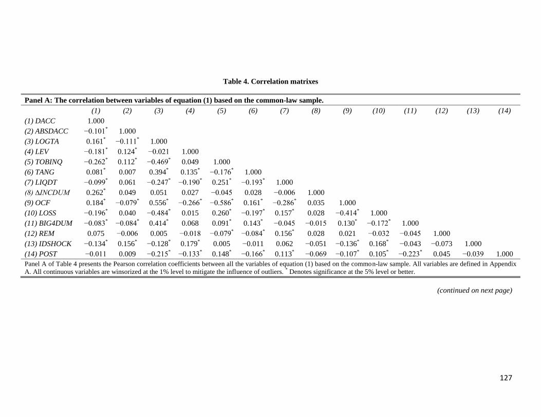
127
Table 4. Correlation matrixes
Panel A: The correlation between variables of equation (1) based on the common-law sample.
(1) (2) (3) (4) (5) (6) (7) (8) (9) (10) (11) (12) (13) (14)
(1) DACC 1.000
(2) ABSDACC −0.101* 1.000
(3) LOGTA 0.161* −0.111
* 1.000
(4) LEV −0.181* 0.124
* −0.021 1.000
(5) TOBINQ −0.262* 0.112
* −0.469
* 0.049 1.000
(6) TANG 0.081* 0.007 0.394
* 0.135
* −0.176
* 1.000
(7) LIQDT −0.099* 0.061 −0.247
* −0.190
* 0.251
* −0.193
* 1.000
(8) ∆INCDUM 0.262* 0.049 0.051 0.027 −0.045 0.028 −0.006 1.000
(9) OCF 0.184* −0.079
* 0.556
* −0.266
* −0.586
* 0.161
* −0.286
* 0.035 1.000
(10) LOSS −0.196* 0.040 −0.484
* 0.015 0.260
* −0.197
* 0.157
* 0.028 −0.414
* 1.000
(11) BIG4DUM −0.083* −0.084
* 0.414
* 0.068 0.091
* 0.143
* −0.045 −0.015 0.130
* −0.172
* 1.000
(12) REM 0.075 −0.006 0.005 −0.018 −0.079* −0.084
* 0.156
* 0.028 0.021 −0.032 −0.045 1.000
(13) IDSHOCK −0.134* 0.156
* −0.128
* 0.179
* 0.005 −0.011 0.062 −0.051 −0.136
* 0.168
* −0.043 −0.073 1.000
(14) POST −0.011 0.009 −0.215* −0.133
* 0.148
* −0.166
* 0.113
* −0.069 −0.107
* 0.105
* −0.223
* 0.045 −0.039 1.000
Panel A of Table 4 presents the Pearson correlation coefficients between all the variables of equation (1) based on the common-law sample. All variables are defined in Appendix
A. All continuous variables are winsorized at the 1% level to mitigate the influence of outliers. * Denotes significance at the 5% level or better.
(continued on next page)
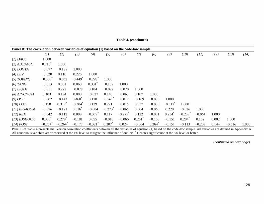
128
Table 4. (continued)
Panel B: The correlation between variables of equation (1) based on the code-law sample.
(1) (2) (3) (4) (5) (6) (7) (8) (9) (10) (11) (12) (13) (14)
(1) DACC 1.000
(2) ABSDACC 0.718* 1.000
(3) LOGTA −0.077 −0.188 1.000
(4) LEV −0.020 0.110 0.226 1.000
(5) TOBINQ −0.303* −0.052 −0.449
* −0.298
* 1.000
(6) TANG −0.013 0.061 0.060 0.331* −0.137 1.000
(7) LIQDT −0.011 0.222 −0.078 0.104 −0.022 −0.070 1.000
(8) ∆INCDUM 0.103 0.194 0.080 −0.027 0.148 −0.063 0.107 1.000
(9) OCF −0.002 −0.143 0.460* 0.128 −0.561
* −0.012 −0.109 −0.070 1.000
(10) LOSS 0.158 0.317* −0.304
* 0.139 0.221 −0.015 0.037 −0.030 −0.517
* 1.000
(11) BIG4DUM −0.076 −0.121 0.516* −0.004 −0.273
* −0.065 0.004 −0.060 0.220 −0.026 1.000
(12) REM −0.042 −0.112 0.009 −0.379* 0.117 −0.275
* 0.122 −0.031 0.234
* −0.238
* −0.064 1.000
(13) IDSHOCK 0.300* 0.279
* −0.181 0.055 −0.018 −0.066 0.251
* −0.158 −0.151 0.284
* 0.152 0.002 1.000
(14) POST −0.274* −0.264
* −0.177 −0.321
* 0.307
* 0.024 −0.064 0.364
* −0.151 −0.113 −0.207 0.144 −0.516 1.000
Panel B of Table 4 presents the Pearson correlation coefficients between all the variables of equation (1) based on the code-law sample. All variables are defined in Appendix A.
All continuous variables are winsorized at the 1% level to mitigate the influence of outliers. * Denotes significance at the 5% level or better.
(continued on next page)

129
Table 4. (continued)
Panel C: The correlation between variables of equation (2) based on the common-law sample.
(1) (2) (3) (4) (5) (6) (7) (8) (9) (10) (11) (12) (13) (14)
(1) CAR[−2;+2] 1.000
(2) LOGISSUE −0.066* 1.000
(3) LOGTA −0.100* 0.693* 1.000
(4) LEV 0.059 −0.007 0.044 1.000
(5) ROA −0.048 0.346* 0.493* −0.236* 1.000
(6) TOBINQ 0.003 −0.198* −0.399* −0.039 −0.446* 1.000
(7) TANG −0.086* 0.244* 0.362* 0.188* 0.157* −0.190* 1.000
(8) LIQDT 0.019 0.040 −0.254* −0.252* −0.147* 0.263* −0.229* 1.000
(9) RND 0.060 −0.016 −0.208* −0.043 −0.259* 0.385* −0.162* 0.340* 1.000
(10) SDEBIT −0.008 −0.018 −0.213* 0.114* −0.174* 0.314* −0.062 0.072* 0.028 1.000
(11) DIVDUM −0.099* 0.349* 0.553* 0.141* 0.301* −0.216* 0.157* −0.245* −0.176* −0.069* 1.000
(12) DAYS 0.042 −0.111* −0.043 −0.052 0.008 −0.039 −0.033 0.006 −0.008 0.011 −0.046 1.000
(13) LOSS 0.098* −0.330* −0.490* −0.060 −0.429* 0.245* −0.191* 0.185* 0.193* 0.077* −0.458* 0.058 1.000
(14) POST 0.019 −0.110* −0.167* −0.096* −0.082* 0.001 −0.138* 0.096* −0.001 −0.088* −0.089* 0.051 0.065* 1.000
Panel C of Table 4 presents the Pearson correlation coefficients between all the variables of equation (2) based on the common-law sample. All variables are defined in Appendix
A. All continuous variables are winsorized at the 1% level to mitigate the influence of outliers. * Denotes significance at the 5% level or better.
(continued on next page)

130
Table 4. (continued)
Panel D: The correlation between variables of equation (2) based on the code-law sample.
(1) (2) (3) (4) (5) (6) (7) (8) (9) (10) (11) (12) (13) (14)
(1) CAR[−2;+2] 1.000
(2) LOGISSUE −0.086 1.000
(3) LOGTA −0.122 0.826* 1.000
(4) LEV −0.070 0.146 0.276* 1.000
(5) ROA 0.031 0.183* 0.389* 0.164 1.000
(6) TOBINQ 0.060 −0.203* −0.387* −0.375* −0.287* 1.000
(7) TANG −0.018 0.087 0.167 0.255* 0.110 −0.255* 1.000
(8) LIQDT −0.056 −0.120 −0.239* −0.339* −0.457* 0.226* −0.166 1.000
(9) RND −0.108 −0.097 −0.165 −0.231* −0.202* 0.304* −0.232* −0.050 1.000
(10) SDEBIT −0.028 −0.090 −0.247* −0.155 −0.807* 0.117 −0.076 0.554* −0.020 1.000
(11) DIVDUM −0.008 0.413* 0.536* 0.045 0.270* −0.191* 0.120 −0.196* −0.201* −0.095 1.000
(12) DAYS 0.065 −0.341* −0.265* −0.048 0.020 −0.034 0.131 0.027 −0.074 −0.117 −0.231* 1.000
(13) LOSS 0.004 −0.176* −0.332* −0.010 −0.457* 0.267* −0.080 0.153 0.324* 0.116 −0.402* 0.085 1.000
(14) POST 0.254* −0.057 −0.102 −0.171 0.083 −0.016 0.196* −0.124 0.024 −0.113 0.139 0.273* 0.028 1.000
Panel D of Table 4 presents the Pearson correlation coefficients between all the variables of equation (2) based on the code-law sample. All variables are defined in Appendix A.
All continuous variables are winsorized at the 1% level to mitigate the influence of outliers. * Denotes significance at the 5% level or better.

131
Table 5. The change in the signed/absolute discretionary accruals before issuing SEOs following IFRS adoption (H1)
Common-law Code-law All Common-law Code-law All
DACC DACC DACC ABSDACC ABSDACC ABSDACC
POST 0.0004 −0.0667***
−0.0006 −0.0015 −0.0496***
−0.0028
(0.03) (−3.54) (−0.04) (−0.16) (−3.39) (−0.30)
CODE 0.0824***
−0.0219
(3.29) (−1.16)
POST*CODE −0.0961***
−0.0351**
(−3.80) (−2.07)
LOGTA 0.0048 −0.0043 0.0034 −0.0043 −0.0051 −0.0043*
(1.18) (−0.85) (0.97) (−1.56) (−1.25) (−1.82)
LEV −0.0881***
−0.0984* −0.0845
*** 0.0389
*** −0.0299 0.0377
***
(−4.20) (−2.00) (−4.13) (2.89) (−0.75) (2.89)
TOBINQ −0.0097**
−0.0383***
−0.0107***
0.0040 −0.0070 0.0037
(−2.51) (−4.38) (−2.78) (1.16) (−1.10) (1.09)
TANG 0.0311 0.0023 0.0370* 0.0127 0.0087 0.0114
(1.44) (0.07) (1.86) (0.96) (0.35) (0.95)
LIQDT −0.0870**
−0.1668 −0.0834**
0.0426 0.2054 0.0412
(−2.23) (−0.78) (−2.16) (1.52) (1.67) (1.49)
∆INCDUM 0.0863***
0.0464**
0.0834***
0.0102 0.0320**
0.0124*
(7.52) (2.62) (7.89) (1.27) (2.45) (1.67)
OCF −0.0392 −0.0487 −0.0327 0.0245 0.0233 0.0238
(−1.55) (−0.65) (−1.33) (1.61) (0.48) (1.63)
LOSS −0.0563***
0.0258 −0.0449***
−0.0044 0.0241 −0.0011
(−4.18) (1.19) (−3.78) (−0.52) (1.50) (−0.15)
BIG4DUM −0.0144 −0.0186 −0.0160 −0.0143 −0.0115 −0.0135*
(−1.03) (−0.89) (−1.29) (−1.64) (−0.77) (−1.73)
RIGHTDUM −0.0520**
−0.0344**
−0.0479**
0.0045 −0.0102 −0.0004
(−2.06) (−2.41) (−2.53) (0.23) (−0.98) (−0.03)
(continued on next page)

132
Table 5. (continued)
Common-law Code-law All Common-law Code-law All
DACC DACC DACC ABSDACC ABSDACC ABSDACC
PUBLICDUM −0.0129
−0.0157 0.0086
0.0066
(−0.53)
(−0.65) (0.59)
(0.47)
REM 0.0166 0.0356 0.0162 0.0006 0.0205 0.0017
(0.74) (0.84) (0.75) (0.04) (0.70) (0.11)
Intercept 0.0953* 0.3362
*** 0.1036
* 0.1263
*** 0.2111
*** 0.1771
***
(1.96) (5.63) (1.95) (3.76) (4.13) (5.45)
N 645 75 720 645 75 720
Adjusted-R2 20.61% 25.17% 19.50% 7.28% 24.05% 8.91%
Table 5 presents results on the change in the signed/absolute discretionary accruals before issuing SEOs following IFRS adoption
among common-law and code-law firms between 2002 and 2008, excluding 2005, using a difference-in-differences research design.
The first two columns of Table 5 report results from the OLS regressions of signed discretionary accruals on a set of firm
characteristics and the IFRS dummy, using the common-law and the code-law samples respectively, between 2002 and 2008,
excluding 2005. The third column of Table 5 reports results from the OLS regression of signed discretionary accruals on a set of firm
characteristics and the difference-in-differences dummies, using the full sample between 2002 and 2008, excluding 2005. Column 4
and column 5 Table 5 report results from the OLS regressions of absolute discretionary accruals on a set of firm characteristics and the
IFRS dummy, using the common-law and the code-law samples respectively, between 2002 and 2008, excluding 2005. The third
column of Table 5 reports results from the OLS regression of absolute discretionary accruals on a set of firm characteristics and the
difference-in-differences dummies, using the full sample between 2002 and 2008, excluding 2005. All variables are defined in
Appendix A. All continuous variables are winsorized at the 1% level to mitigate the influence of outliers. All regressions include year
and industry fixed effects. The t-statistics, presented in parentheses below the coefficients, are calculated using White (1980) standard
errors. *,
**,
*** Denote significance at the 10%, 5%, and 1% levels, respectively.

133
Table 6. The change in discretionary accruals after controlling for Idiosyncratic Economic Shocks (H1)
Common-law Code-law All Common-law Code-law All
DACC DACC DACC ABSDACC ABSDACC ABSDACC
POST −0.0006 −0.0520**
−0.0016 −0.0004 −0.0465***
−0.0015
(−0.04) (−2.35) (−0.11) (−0.04) (−2.98) (−0.15)
CODE 0.0909***
−0.0331*
(3.42) (−1.80)
POST*CODE −0.1046***
−0.024
(−3.86) (−1.40)
LOGTA 0.0044 −0.0033 0.0029 −0.0039 −0.0049 −0.0037
(1.10) (−0.61) (0.86) (−1.45) (−1.18) (−1.61)
LEV −0.0833***
−0.0873 −0.0812***
0.0340**
−0.0275 0.0334**
(−3.97) (−1.66) (−3.98) (2.49) (−0.66) (2.55)
TOBINQ −0.0102**
−0.0384***
−0.0111***
0.0045 −0.0070 0.0042
(−2.56) (−4.05) (−2.80) (1.27) (−1.09) (1.21)
TANG 0.0325 −0.0037 0.0380* 0.0112 0.0074 0.0101
(1.51) (−0.11) (1.92) (0.86) (0.29) (0.85)
LIQDT −0.0810**
−0.2287 −0.0792**
0.0364 0.1921 0.0357
(−2.23) (−1.14) (−2.18) (1.43) (1.42) (1.41)
∆INCDUM 0.0846***
0.0448**
0.0823***
0.0120 0.0316**
0.0138*
(7.34) (2.66) (7.79) (1.52) (2.38) (1.90)
OCF −0.0398 −0.0389 −0.0332 0.0252* 0.0254 0.0246
*
(−1.59) (−0.51) (−1.36) (1.69) (0.50) (1.71)
LOSS −0.0527***
0.0214 −0.0420***
−0.0083 0.0231 −0.0049
(−3.79) (0.99) (−3.44) (−0.94) (1.46) (−0.64)
BIG4DUM −0.0137 −0.0265 −0.0148 −0.0150* −0.0132 −0.0150
*
(−0.97) (−1.17) (−1.17) (−1.71) (−0.86) (−1.89)
RIGHTDUM −0.0532**
−0.0309**
−0.0496**
0.0058 −0.0095 0.0019
(−2.08) (−2.07) (−2.58) (0.30) (−0.85) (0.13)
(continued on next page)

134
Table 6. (continued)
Common-law Code-law All Common-law Code-law All
DACC DACC DACC ABSDACC ABSDACC ABSDACC
PUBLICDUM −0.0152 −0.0178 0.011 0.0093
(−0.63) (−0.74) (0.76) (0.66)
REM 0.0140 0.0265 0.0145 0.0034 0.0185 0.0040
(0.60) (0.63) (0.66) (0.21) (0.63) (0.26)
IDSHOCK −0.0208 0.0199 −0.0161 0.0217* 0.0042 0.0211
**
(−1.25) (1.17) (−1.10) (1.78) (0.30) (1.98)
Intercept 0.1073* 0.2053
*** 0.1134
*** 0.1701
*** 0.1154
* 0.1184
***
(1.82) (2.79) (2.68) (4.51) (1.98) (3.99)
N 645 75 720 645 75 720
Adjusted-R2 25.05% 29.64% 24.32% 7.88% 27.76% 10.40%
Table 6 presents results on the change in the signed/absolute discretionary accruals before issuing SEOs following IFRS adoption
among common-law and code-law firms between 2002 and 2008, excluding 2005, using a difference-in-differences research design.
These regressions include a proxy for Idiosyncratic Economic Shocks as computed in Owens, Wu and Zimmerman (2016).
The first two columns of Table 6 report results from the OLS regressions of signed discretionary accruals on a set of firm
characteristics and the IFRS dummy, while including a proxy for business model shock, using the common-law and the code-law
samples respectively, between 2002 and 2008, excluding 2005. The third column of Table 6 reports results from the OLS regression
of signed discretionary accruals on a set of firm characteristics and the difference-in-differences dummies, while including a proxy
for idiosyncratic business model shock, using the full sample between 2002 and 2008, excluding 2005. Column 4 and column 5 in
Table 6 report results from the OLS regressions of absolute discretionary accruals on a set of firm characteristics and the IFRS
dummy, while including a proxy for business model shock, using the common-law and the code-law samples respectively, between
2002 and 2008, excluding 2005. The third column of Table 6 reports results from the OLS regression of absolute discretionary
accruals on a set of firm characteristics and the difference-in-differences dummies, while including a proxy for idiosyncratic
business model shock, using the full sample between 2002 and 2008, excluding 2005. All variables are defined in Appendix A. All
continuous variables are winsorized at the 1% level to mitigate the influence of outliers. All regressions include year and industry
fixed effects. The t-statistics, presented in parentheses below the coefficients, are calculated using White (1980) standard errors. *,
**,
*** Denote significance at the 10%, 5%, and 1% levels, respectively.

135
Table 7. The change in the market reaction to issuing SEOs following IFRS adoption (H2)
Common-law Code-law All
CAR[−2,+2] CAR[−2,+2] CAR[−2,+2]
POST 0.0014 0.0260***
0.0014
(0.41) (4.23) (0.42)
CODE −0.0175***
(−3.28)
POST*CODE 0.0234***
(3.60)
LOGISSUE 0.0006 −0.0017 0.0005
(0.55) (−0.97) (0.46)
LOGTA −0.0012 −0.0013 −0.0013
(−0.84) (−0.69) (−1.02)
LEV 0.0082 0.0082 0.0083
(1.21) (0.63) (1.31)
ROA 0.0016 0.0042 0.0013
(0.49) (0.13) (0.43)
TOBINQ −0.0005 0.0029 −0.0004
(−0.70) (1.28) (−0.59)
TANG −0.0155***
−0.0305**
−0.0161***
(−2.62) (−2.04) (−2.91)
LIQDT −0.0038 −0.0197 −0.0024
(−0.40) (−0.88) (−0.27)
RND 0.0340 −0.0742* 0.0282
(1.41) (−1.81) (1.25)
SDEBIT −0.0004 0.0007 −0.0004
(−0.81) (0.15) (−0.96)
DIVDUM −0.0091* 0.0004 −0.0069
(−1.68) (0.09) (−1.53)
(continued on next page)
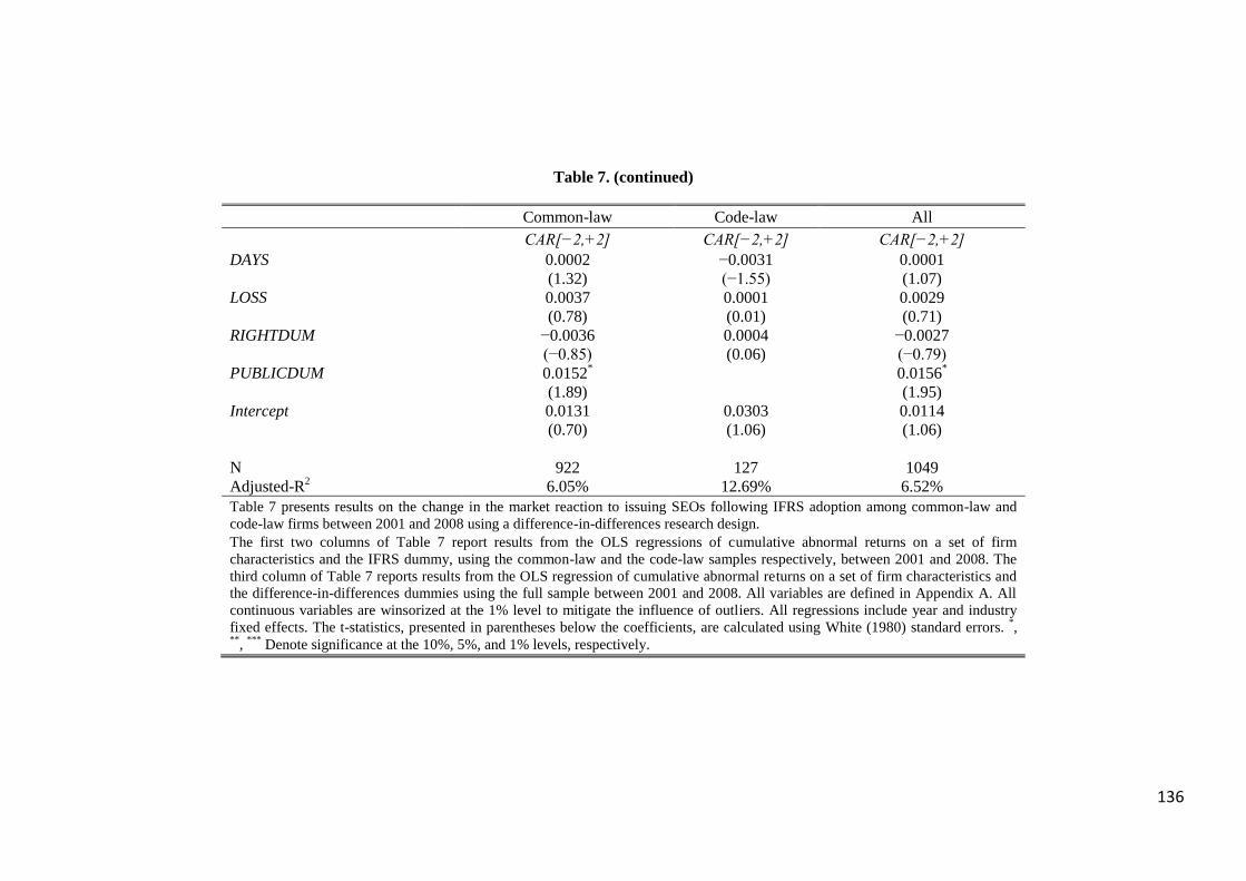
136
Table 7. (continued)
Common-law Code-law All
CAR[−2,+2] CAR[−2,+2] CAR[−2,+2]
DAYS 0.0002 −0.0031 0.0001
(1.32) (−1.55) (1.07)
LOSS 0.0037 0.0001 0.0029
(0.78) (0.01) (0.71)
RIGHTDUM −0.0036 0.0004 −0.0027
(−0.85) (0.06) (−0.79)
PUBLICDUM 0.0152*
0.0156*
(1.89)
(1.95)
Intercept 0.0131 0.0303 0.0114
(0.70) (1.06) (1.06)
N 922 127 1049
Adjusted-R2 6.05% 12.69% 6.52%
Table 7 presents results on the change in the market reaction to issuing SEOs following IFRS adoption among common-law and
code-law firms between 2001 and 2008 using a difference-in-differences research design.
The first two columns of Table 7 report results from the OLS regressions of cumulative abnormal returns on a set of firm
characteristics and the IFRS dummy, using the common-law and the code-law samples respectively, between 2001 and 2008. The
third column of Table 7 reports results from the OLS regression of cumulative abnormal returns on a set of firm characteristics and
the difference-in-differences dummies using the full sample between 2001 and 2008. All variables are defined in Appendix A. All
continuous variables are winsorized at the 1% level to mitigate the influence of outliers. All regressions include year and industry
fixed effects. The t-statistics, presented in parentheses below the coefficients, are calculated using White (1980) standard errors. *,
**,
*** Denote significance at the 10%, 5%, and 1% levels, respectively.
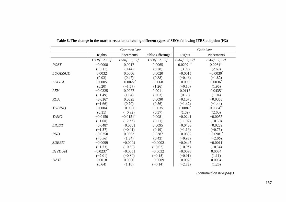
137
Table 8. The change in the market reaction to issuing different types of SEOs following IFRS adoption (H2)
Common-law Code-law
Rights Placements Public Offerings Rights Placements
CAR[−2,+2] CAR[−2,+2] CAR[−2,+2] CAR[−2,+2] CAR[−2,+2]
POST −0.0008 0.0017 0.0065 0.0297***
0.0264**
(−0.11) (0.44) (0.28) (3.09) (2.69)
LOGISSUE 0.0032 0.0006 0.0020 −0.0015 −0.0030*
(0.93) (0.47) (0.38) (−0.46) (−1.82)
LOGTA 0.0005 −0.0027* 0.0068 −0.0003 0.0036
*
(0.20) (−1.77) (1.26) (−0.10) (1.96)
LEV −0.0325 0.0077 0.0011 0.0117 0.0435*
(−1.49) (1.04) (0.03) (0.85) (1.94)
ROA −0.0167 0.0025 0.0090 −0.1076 −0.0353
(−1.66) (0.70) (0.56) (−1.62) (−1.44)
TOBINQ 0.0004 −0.0006 0.0035 0.0087* 0.0084
**
(0.11) (−0.82) (0.37) (1.69) (2.60)
TANG −0.0150 −0.0151**
0.0081 −0.0241 −0.0055
(−1.08) (−2.55) (0.21) (−1.02) (−0.30)
LIQDT −0.0487 −0.0001 0.0095 −0.0453 −0.0239
(−1.37) (−0.01) (0.19) (−1.16) (−0.75)
RND −0.0250 0.0363 0.0387 −0.0502 −0.0981*
(−0.56) (1.34) (0.43) (−0.93) (−2.06)
SDEBIT −0.0099 −0.0004 −0.0002 −0.0445 −0.0011
(−1.53) (−0.80) (−0.02) (−0.95) (−0.34)
DIVDUM −0.0237**
−0.0051 −0.0032 −0.0096 0.0084
(−2.01) (−0.80) (−0.15) (−0.91) (1.11)
DAYS 0.0018 0.0006 −0.0009 −0.0023 0.0004
(0.64) (1.10) (−0.14) (−2.32) (1.26)
(continued on next page)

138
Table 8. (continued)
Common-law Code-law
Rights Placements Public Offerings Rights Placements
CAR[−2,+2] CAR[−2,+2] CAR[−2,+2] CAR[−2,+2] CAR[−2,+2]
LOSS −0.0126 0.0025 0.0541* −0.0224 −0.0075
(−1.27) (0.46) (1.81) (−1.63) (−0.68)
Intercept 0.0125 0.0233 −0.0043 0.0355 −0.0770**
(0.32) (1.61) (−0.03) (0.97) (−2.65)
N 84 760 78 78 49
Adjusted-R2 8.14% 5.27% 12.40% 21.51% 24.61%
Table 8 presents results on the change in the market reaction to issuing different types of SEO offerings following IFRS adoption
among common-law and code-law firms between 2001 and 2008.
The first three columns of Table 8 report results from the OLS regressions of cumulative abnormal returns on a set of firm
characteristics and the IFRS dummy for each offering technique in the common-law sample, between 2001 and 2008. The last two
columns of Table 8 report results from the OLS regression of cumulative abnormal returns on a set of firm characteristics and the
IFRS dummy for each offering technique in the code-law sample, between 2001 and 2008. All variables are defined in Appendix A.
All continuous variables are winsorized at the 1% level to mitigate the influence of outliers. All regressions include year and
industry fixed effects. The t-statistics, presented in parentheses below the coefficients, are calculated using White (1980) standard
errors. *,
**,
*** Denote significance at the 10%, 5%, and 1% levels, respectively.

139
Table 9. The change in the market reaction to Rights and Placements following IFRS adoption (H2)
Rights Placements
CAR[-2,+2] CAR[-2,+2]
POST −0.0025 0.0013
(−0.35) (0.32)
CODE −0.0191**
−0.0160**
(−2.59) (−2.24)
POST*CODE 0.0300***
0.0184*
(3.27) (1.82)
LOGISSUE 0.0025 0.0003
(1.00) (0.22)
LOGTA −0.0012 −0.0024*
(−0.65) (−1.77)
LEV −0.0172 0.0125**
(−1.30) (2.08)
ROA −0.0221***
0.0036
(−2.96) (1.04)
TOBINQ 0.0019 −0.0006
(0.65) (−0.86)
TANG −0.0103 −0.0167***
(−1.16) (−3.34)
LIQDT −0.0378**
0.0001
(−2.45) (0.01)
RND −0.0068 0.0177
(−0.32) (0.81)
SDEBIT −0.0137***
−0.0005
(−3.10) (−1.42)
DIVDUM −0.0166**
−0.0034
(−2.31) (−0.61)
(continued on next page)
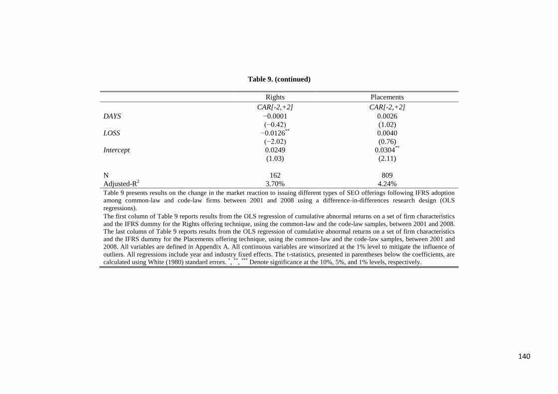
140
Table 9. (continued)
Rights Placements
CAR[-2,+2] CAR[-2,+2]
DAYS −0.0001 0.0026
(−0.42) (1.02)
LOSS −0.0126**
0.0040
(−2.02) (0.76)
Intercept 0.0249 0.0304**
(1.03) (2.11)
N 162 809
Adjusted-R2 3.70% 4.24%
Table 9 presents results on the change in the market reaction to issuing different types of SEO offerings following IFRS adoption
among common-law and code-law firms between 2001 and 2008 using a difference-in-differences research design (OLS
regressions).
The first column of Table 9 reports results from the OLS regression of cumulative abnormal returns on a set of firm characteristics
and the IFRS dummy for the Rights offering technique, using the common-law and the code-law samples, between 2001 and 2008.
The last column of Table 9 reports results from the OLS regression of cumulative abnormal returns on a set of firm characteristics
and the IFRS dummy for the Placements offering technique, using the common-law and the code-law samples, between 2001 and
2008. All variables are defined in Appendix A. All continuous variables are winsorized at the 1% level to mitigate the influence of
outliers. All regressions include year and industry fixed effects. The t-statistics, presented in parentheses below the coefficients, are
calculated using White (1980) standard errors. *,
**,
*** Denote significance at the 10%, 5%, and 1% levels, respectively.

141
Table 10. The change in the propensity to issue SEOs following IFRS adoption (H3)
Time period: 2001 - 2008 Time period: 2003 - 2006
Common-law Code-law All Common-law Code-law All
SEODUM SEODUM SEODUM SEODUM SEODUM SEODUM
POST 0.2317***
0.6145***
0.2391***
−0.0559 1.1209***
−0.0508
(2.65) (2.96) (2.74) (−0.40) (3.23) (−0.36)
CODE −0.2686 −0.9683***
(−1.45) (−3.27)
POST*CODE 0.3460 0.9655***
(1.57) (2.70)
LOGTA 0.0150 0.1014**
0.0363 0.1102**
0.2914***
0.1452***
(0.56) (2.22) (1.63) (2.53) (3.39) (4.00)
LEV −0.4549***
−0.6083 −0.4453***
−0.7649***
0.2733 −0.5857***
(−3.67) (−1.20) (−3.82) (−3.33) (0.37) (−2.85)
ROA −0.2678**
−0.5367 −0.2859***
0.0071 0.0628 0.0185
(−2.48) (−1.08) (−2.76) (0.03) (0.05) (0.08)
TOBINQ −0.0171 0.0443 −0.0115 0.0117 −0.2146 0.0126
(−0.83) (0.86) (−0.60) (0.28) (−0.58) (0.32)
TANG 0.0278 0.6651 0.0676 0.0066 0.3720 0.0279
(0.14) (1.20) (0.37) (0.02) (0.48) (0.10)
LIQDT −0.5253**
−0.0585 −0.4285* −0.3654 −1.2259 −0.2536
(−2.24) (−0.06) (−1.90) (−0.93) (−0.71) (−0.67)
RND 0.4213 −2.9503* 0.0817 1.3394
** −0.4405 1.0718
*
(1.03) (−1.92) (0.21) (2.21) (−0.22) (1.90)
DIVDUM −0.1805 −0.4984* −0.2370
** −0.0399 −0.4147 −0.1028
(−1.38) (−1.80) (−2.03) (−0.19) (−0.97) (−0.53)
LOSS 0.2704**
0.3472 0.2890***
0.2885 0.9201* 0.4164
**
(2.33) (1.34) (2.77) (1.47) (1.79) (2.34)
RIGHTDUM −0.3398**
−0.0099 −0.2747**
0.2763 0.1674 0.2666
(−2.24) (−0.04) (−2.27) (1.26) (0.37) (1.45)
(continued on next page)

142
Table 10. (continued)
Time period: 2001 - 2008 Time period: 2003 - 2006
Common-law Code-law All Common-law Code-law All
SEODUM SEODUM SEODUM SEODUM SEODUM SEODUM
PUBLICDUM −0.1541
−0.1545 0.2602
0.2527
(−1.06)
(−1.07) (1.20)
(1.17)
Intercept −0.8263**
−2.1648**
−1.0560***
−1.8955***
−5.3204***
−2.3404***
(−2.07) (−2.51) (−3.02) (−2.79) (−3.07) (−3.98)
N 3101 673 3774 1567 328 1895
Pseudo-R2 4.52% 6.70% 4.96% 5.23% 17.74% 5.02%
Number of Issues 765 125 890 253 48 301
Marginal Effects
POST 4.19%***
9.05%***
4.2%***
-0.72% 10.67%***
-0.63%
CODE
-4.54%
-9.67%***
POST*CODE
6.59%
15.49%**
Table 10 presents results on the change in the propensity to issue SEOs following IFRS adoption among common-law and code-
law firms between 2001 and 2008 and between 2003 and 2006 using a difference-in-differences research design.
The first two columns of Table 10 report results from the Logistic regressions of the SEO dummy on a set of firm characteristics
and the IFRS dummy, using the common-law and the code-law samples respectively, between 2001 and 2008. The third column of
Table 10 reports results from the Logistic regression of the SEO dummy on a set of firm characteristics and the difference-in-
differences dummies, using the full sample between 2001 and 2008. Column 4 and Column 5 of Table 10 report results from the
Logistic regressions of the SEO dummy on a set of firm characteristics and the IFRS dummy, using the common-law and the code-
law samples respectively, between 2003 and 2006. The last column of Table 10 reports results from the Logistic regression of the
SEO dummy on a set of firm characteristics and the difference-in-differences dummies, using the full sample between 2003 and
2006. The table reports the marginal effects for the difference-in-differences dummies at the bottom. All variables are defined in
Appendix A. All continuous variables are winsorized at the 1% level to mitigate the influence of outliers. All regressions include
year and industry fixed effects. The z-statistics, presented in parentheses below the coefficients, are calculated using White (1980)
standard errors. *,
**,
*** Denote significance at the 10%, 5%, and 1% levels, respectively.

143
Table 11. The change in the discretionary accruals prior to SEOs based on matched sample regressions (H1)
Common-law Code-law All
DACC DACC DACC
POST 0.0003 −0.0639***
−0.0027
(0.01) (−2.97) (−0.10)
CODE 0.0819**
(2.52)
POST*CODE −0.0806**
(−2.43)
LOGTA 0.0001 −0.0052 −0.0004
(0.01) (−0.64) (−0.07)
LEV −0.0518 −0.0576 −0.066
(−0.84) (−0.95) (−1.47)
TOBINQ 0.0024 −0.0418***
−0.0066
(0.28) (−4.38) (−0.74)
TANG 0.0829 −0.0272 0.032
(1.52) (−0.62) (0.92)
LIQDT 0.0147 −0.1914 0.0773
(0.07) (−0.85) (0.53)
∆INCDUM 0.0635**
0.0477**
0.0601***
(2.06) (2.43) (3.67)
OCF 0.0991 −0.0758 0.0617
(1.06) (−0.88) (0.93)
LOSS −0.0442 0.0140 −0.0210
(−0.91) (0.59) (−0.94)
BIG4DUM 0.0035 −0.0196 −0.0003
(0.08) (−0.92) (−0.01)
RIGHTDUM −0.0606 −0.0389**
−0.0531***
(−1.34) (−2.37) (−2.78)
(continued on next page)
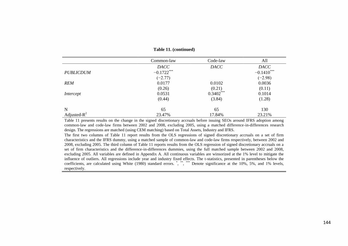
144
Table 11. (continued)
Common-law Code-law All
DACC DACC DACC
PUBLICDUM −0.1722***
−0.1410***
(−2.77)
(−2.98)
REM 0.0177 0.0102 0.0036
(0.26) (0.21) (0.11)
Intercept 0.0531 0.3402***
0.1014
(0.44) (3.84) (1.28)
N 65 65 130
Adjusted-R2 23.47% 17.84% 23.21%
Table 11 presents results on the change in the signed discretionary accruals before issuing SEOs around IFRS adoption among
common-law and code-law firms between 2002 and 2008, excluding 2005, using a matched difference-in-differences research
design. The regressions are matched (using CEM matching) based on Total Assets, Industry and IFRS.
The first two columns of Table 11 report results from the OLS regressions of signed discretionary accruals on a set of firm
characteristics and the IFRS dummy, using a matched sample of common-law and code-law firms respectively, between 2002 and
2008, excluding 2005. The third column of Table 11 reports results from the OLS regression of signed discretionary accruals on a
set of firm characteristics and the difference-in-differences dummies, using the full matched sample between 2002 and 2008,
excluding 2005. All variables are defined in Appendix A. All continuous variables are winsorized at the 1% level to mitigate the
influence of outliers. All regressions include year and industry fixed effects. The t-statistics, presented in parentheses below the
coefficients, are calculated using White (1980) standard errors. *,
**,
*** Denote significance at the 10%, 5%, and 1% levels,
respectively.
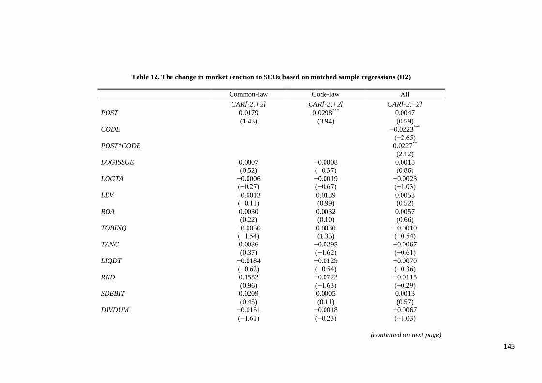
145
Table 12. The change in market reaction to SEOs based on matched sample regressions (H2)
Common-law Code-law All
CAR[-2,+2] CAR[-2,+2] CAR[-2,+2]
POST 0.0179 0.0298***
0.0047
(1.43) (3.94) (0.59)
CODE −0.0223***
(−2.65)
POST*CODE 0.0227**
(2.12)
LOGISSUE 0.0007 −0.0008 0.0015
(0.52) (−0.37) (0.86)
LOGTA −0.0006 −0.0019 −0.0023
(−0.27) (−0.67) (−1.03)
LEV −0.0013 0.0139 0.0053
(−0.11) (0.99) (0.52)
ROA 0.0030 0.0032 0.0057
(0.22) (0.10) (0.66)
TOBINQ −0.0050 0.0030 −0.0010
(−1.54) (1.35) (−0.54)
TANG 0.0036 −0.0295 −0.0067
(0.37) (−1.62) (−0.61)
LIQDT −0.0184 −0.0129 −0.0070
(−0.62) (−0.54) (−0.36)
RND 0.1552 −0.0722 −0.0115
(0.96) (−1.63) (−0.29)
SDEBIT 0.0209 0.0005 0.0013
(0.45) (0.11) (0.57)
DIVDUM −0.0151 −0.0018 −0.0067
(−1.61) (−0.23) (−1.03)
(continued on next page)
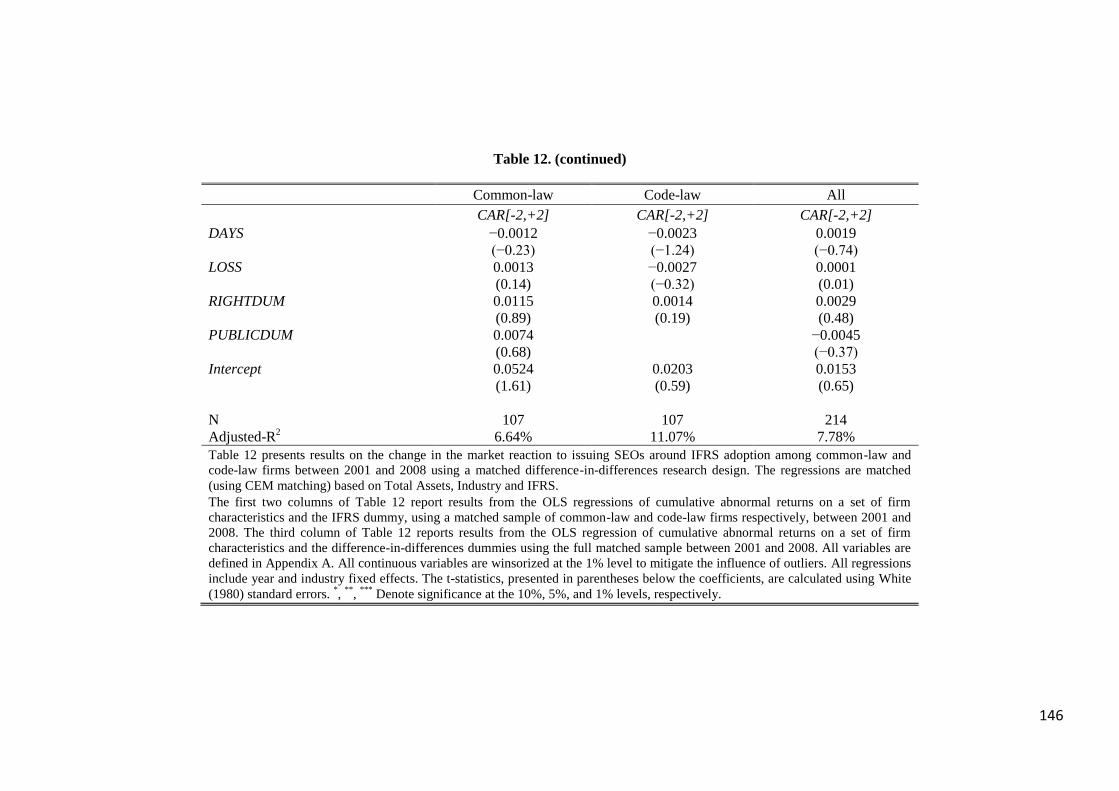
146
Table 12. (continued)
Common-law Code-law All
CAR[-2,+2] CAR[-2,+2] CAR[-2,+2]
DAYS −0.0012 −0.0023 0.0019
(−0.23) (−1.24) (−0.74)
LOSS 0.0013 −0.0027 0.0001
(0.14) (−0.32) (0.01)
RIGHTDUM 0.0115 0.0014 0.0029
(0.89) (0.19) (0.48)
PUBLICDUM 0.0074
−0.0045
(0.68)
(−0.37)
Intercept 0.0524 0.0203 0.0153
(1.61) (0.59) (0.65)
N 107 107 214
Adjusted-R2 6.64% 11.07% 7.78%
Table 12 presents results on the change in the market reaction to issuing SEOs around IFRS adoption among common-law and
code-law firms between 2001 and 2008 using a matched difference-in-differences research design. The regressions are matched
(using CEM matching) based on Total Assets, Industry and IFRS.
The first two columns of Table 12 report results from the OLS regressions of cumulative abnormal returns on a set of firm
characteristics and the IFRS dummy, using a matched sample of common-law and code-law firms respectively, between 2001 and
2008. The third column of Table 12 reports results from the OLS regression of cumulative abnormal returns on a set of firm
characteristics and the difference-in-differences dummies using the full matched sample between 2001 and 2008. All variables are
defined in Appendix A. All continuous variables are winsorized at the 1% level to mitigate the influence of outliers. All regressions
include year and industry fixed effects. The t-statistics, presented in parentheses below the coefficients, are calculated using White
(1980) standard errors. *,
**,
*** Denote significance at the 10%, 5%, and 1% levels, respectively.

147
Table 13. The change in the propensity to issue SEOs based on matched sample regressions (H3)
Common-law Code-law All
SEODUM SEODUM SEODUM
POST −0.2016 0.6771***
−0.2044
(−1.00) (3.01) (−1.02)
CODE −0.4218*
(−1.69)
POST*CODE 0.8545***
(2.74)
LOGTA −0.0945 0.0684 0.0011
(−1.56) (1.43) (0.03)
LEV −0.6127* −0.5791 −0.4892
*
(−1.76) (−1.12) (−1.92)
ROA −0.1847 −0.4869 −0.2166
(−0.56) (−0.97) (−0.85)
TOBINQ −0.0882 0.0582 −0.0303
(−1.50) (1.13) (−0.80)
TANG 0.4513 0.8758 0.464
(0.91) (1.51) (1.29)
LIQDT 0.0661 0.0427 0.3253
(0.09) (0.05) (0.60)
RND 0.9103 −2.9778* −0.821
(0.63) (−1.90) (−0.85)
DIVDUM 0.0185 −0.4312 −0.1944
(0.07) (−1.46) (−0.99)
LOSS 0.2936 0.3768 0.3522*
(1.08) (1.36) (1.87)
RIGHTDUM −0.0805 0.0858 −0.0308
(−0.28) (0.34) (−0.18)
(continued on next page)

148
Table 13. (continued)
Common-law Code-law All
SEODUM SEODUM SEODUM
PUBLICDUM −0.1379 −0.1423
(−0.40) (−0.42)
Intercept 0.5106 −1.6637* −0.7079
(0.54) (−1.79) (−1.11)
N 602 602 1204
Pseudo-R2 5.25% 7.32% 5.09%
Number of Issues 125 110 235
Marginal Effects
POST −3.19% 9.73%*** −3.18%
CODE
−6.55%*
POST*CODE
14.87%***
Table 13 presents results on the change in the propensity to issue SEOs around IFRS adoption among common-law and code-law
firms between 2001 and 2008 using a matched difference-in-differences research design. The regressions are matched (using CEM
matching) based on Total Assets, Industry and IFRS.
The first two columns of Table 13 report results from the Logistic regressions of the SEO dummy on a set of firm characteristics and
the IFRS dummy, using matched samples from common-law and code-law firms respectively, between 2001 and 2008. The third
column of Table 13 reports results from the Logistic regression of the SEO dummy on a set of firm characteristics and the
difference-in-differences dummies, using the full matched sample between 2001 and 2008. The table reports the marginal effects for
the difference-in-differences dummies at the bottom. All variables are defined in Appendix A. All continuous variables are
winsorized at the 1% level to mitigate the influence of outliers. All regressions include year and industry fixed effects. The z-
statistics, presented in parentheses below the coefficients, are calculated using White (1980) standard errors. *,
**,
*** Denote
significance at the 10%, 5%, and 1% levels, respectively.
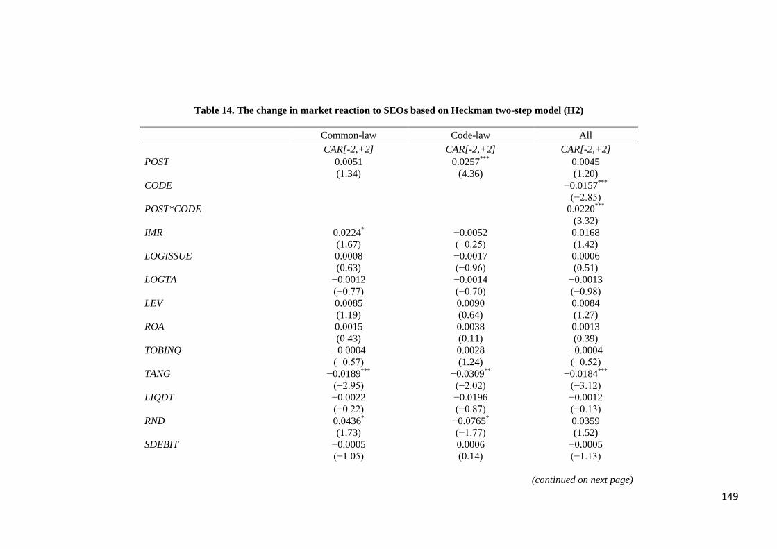
149
Table 14. The change in market reaction to SEOs based on Heckman two-step model (H2)
Common-law Code-law All
CAR[-2,+2] CAR[-2,+2] CAR[-2,+2]
POST 0.0051 0.0257***
0.0045
(1.34) (4.36) (1.20)
CODE −0.0157***
(−2.85)
POST*CODE 0.0220***
(3.32)
IMR 0.0224* −0.0052 0.0168
(1.67) (−0.25) (1.42)
LOGISSUE 0.0008 −0.0017 0.0006
(0.63) (−0.96) (0.51)
LOGTA −0.0012 −0.0014 −0.0013
(−0.77) (−0.70) (−0.98)
LEV 0.0085 0.0090 0.0084
(1.19) (0.64) (1.27)
ROA 0.0015 0.0038 0.0013
(0.43) (0.11) (0.39)
TOBINQ −0.0004 0.0028 −0.0004
(−0.57) (1.24) (−0.52)
TANG −0.0189***
−0.0309**
−0.0184***
(−2.95) (−2.02) (−3.12)
LIQDT −0.0022 −0.0196 −0.0012
(−0.22) (−0.87) (−0.13)
RND 0.0436* −0.0765
* 0.0359
(1.73) (−1.77) (1.52)
SDEBIT −0.0005 0.0006 −0.0005
(−1.05) (0.14) (−1.13)
(continued on next page)

150
Table 14. (continued)
Common-law Code-law All
CAR[-2,+2] CAR[-2,+2] CAR[-2,+2]
DIVDUM −0.0126**
0.0006 −0.0094*
(−2.02) (0.09) (−1.82)
DAYS 0.0003 −0.0061 0.0001
(1.23) (−1.45) (1.01)
LOSS 0.0086 −0.0009 0.0065
(1.43) (−0.09) (1.26)
RIGHTDUM −0.0040 0.0005 −0.0032
(−0.92) (0.08) (−0.89)
PUBLICDUM 0.0152*
0.0155*
(1.87)
(1.93)
Intercept −0.0195 0.0371 −0.0279
(−0.76) (0.97) (−0.94)
N 922 127 1049
Adjusted-R2 6.26% 12.36% 6.67%
Table 14 presents results on the change in the market reaction to issuing SEOs around IFRS adoption among common-law and
code-law firms between 2001 and 2008, using a difference-in-differences research design, after controlling for self-selection bias
using the Heckman two-step estimator. The variable SALES is used as the exclusion restriction in the first stage.
The first two columns of Table 14 report results from the Heckman two-step regressions of cumulative abnormal returns on a set of
firm characteristics and the IFRS dummy, using the common-law and the code-law samples respectively, between 2001 and 2008.
The third column of Table 14 reports results from the Heckman two-step regression of cumulative abnormal returns on a set of firm
characteristics and the difference-in-differences dummies using the full sample between 2001 and 2008. The Inverse Mills Ratio
(IMR) is calculated using SALES as the exclusion restriction (Kim and Purnandum, 2014). All variables are defined in Appendix A.
All continuous variables are winsorized at the 1% level to mitigate the influence of outliers. All regressions include year and
industry fixed effects. The t-statistics, presented in parentheses below the coefficients, are calculated using White (1980) standard
errors. *,
**,
*** Denote significance at the 10%, 5%, and 1% levels, respectively.

151
Chapter 4
The Bias in Measuring Conditional Conservatism
ABSTRACT: Prior studies have raised concerns about the bias in the asymmetric
timeliness (AT) measure of conditional conservatism (CC) proposed by Basu (1997). This
measure, along with the C_Score measure of Khan & Watts (2009), underpins a large body
of empirical research on CC. Thus, this paper assesses the extent to which the prior
literature needs to be revised because of its reliance on these measures. In exploring this
issue, we replicate prior studies that rely on the AT or the C_Score measures, and then
compare the replicated results with those generated by applying the variance ratio (VR)
measure of CC, proposed by Dutta & Patatoukas (2017). We draw four main conclusions.
First, the AT measure is to some extent associated with the VR measure unconditionally.
Second, the observed variation in the C_Score measure seems more likely to be driven by
the variation in the bias in the AT measure rather than variation in CC. Third, the AT
measure yields similar results to the VR measure in interrupted time-series research
designs that model the change in CC following an exogenous change in accounting policy.
Fourth, the results of prior studies using the AT measure to document cross-sectional
differences in CC are unreliable.
Keywords: Financial Reporting; Conditional Conservatism; Measurement Bias;
Asymmetric Timeliness; Research Design.

152
4.1. Introduction
The literature on conditional conservatism (henceforth CC) is large and still growing (see
the surveys of Mora & Walker, 2015 and Ruch & Taylor, 2015). Most of the empirical
literature on CC relies on the Basu (1997) asymmetric timeliness (hereafter AT) measure
or the Khan & Watts (2009) C_Score measure – a development of the AT measure used to
produce a firm-year measure of CC. Researchers have drawn several important conclusions
about the role of accounting conservatism in capital markets based on the asymmetric
timeliness measures of CC. For instance, prior studies find that CC mitigates bondholder-
shareholder agency problems (Ahmed, Billings, Morton, & Stanford-Harris, 2002), CC is
associated with a lower cost of equity capital (García Lara, García Osma, & Penalva,
2011), and CC is used to resolve ramifications arising from information asymmetry
(LaFond & Watts, 2008). However, recent literature raises serious concerns about potential
bias in the AT measure arising from non-accounting (economic) factors (Dietrich, Muller,
& Riedl, 2007; Givoly, Hayn, & Natarajan, 2007; Patatoukas & Thomas, 2011, 2016). The
main purpose of our study is to help assess the likelihood that prior literature on CC may
need to be revised based on a more appropriate measure. In investigating this matter, we
heed the call of Ball (2016) to revisit previous studies and verify their conclusions using
new methodologies and data. Our findings have particular implications for researchers
interested in testing theories about the costs and benefits of CC.
Dutta & Patatoukas (2017) develop a novel measure for estimating CC, the variance
ratio (hereafter VR), which is the spread between the conditional variance of bad news
accruals and the conditional variance of good news accruals. They show that their measure
does not suffer from the bias implicit in the AT measure. Specifically, whilst the AT
coefficient estimate is biased due to price-scale irregularities, expected component of
returns, cashflow persistence and asymmetric returns distribution, the VR measure proves
to be orthogonal to these confounding factors. That is, the VR measure is not driven by the

153
non-accounting factors that yield spurious evidence of CC when using the AT measure.
Thus, we believe that the VR measure provides an appropriate measure to compare with
the long-standing AT measure.
We start our analysis by reporting new evidence showing that the AT and the VR
measures are associated unconditionally. The unconditional association establishes a level
playing field between both measures in a sense that AT and VR arguably estimate the same
feature of financial reporting. This initial analysis is important because it shows that,
although the AT measure is biased, yet it is likely to indicate the presence of CC when it
exists. The problem with the AT measure is that it is biased towards recognising CC when
it does not exist. In statistical terms, the AT measure gives rise to numerous type 1 errors.
Having shown an unconditional association between the AT and the VR measures, we then
move on to investigate the possibility that the bias in the AT measure, which is not present
in the VR measure, may have led to systematic incorrect conclusions in the CC literature.
We achieve this research objective by conducting two sets of empirical tests. Firstly, we
reconstruct the C_Score measure of Khan & Watts (2009) using the VR measure as the
proxy for CC instead of the AT measure. Secondly, we replicate four influential prior
studies that rely on the AT measure (or the C_Score measure), and then compare the
results of our replications with the results generated by applying the VR measure of CC.
Our first set of tests, relating to the C_Score measure, shows that, whilst AT is strongly
related to the decile ranks of stock price, market-to-book ratio, firm size, leverage and the
C_Score measure, such relations either do not exist or are much weaker for the VR
measure. These findings in turn suggest that the bias in the AT measure also applies to the
C_Score measure because of the similar behavior of AT and C_Score across the decile
ranks of the aforementioned financial variables. In other words, the C_Score measure
arguably captures variations in the bias in the AT measure rather actual variations in CC.
In the second set of tests, we first replicate four well known journal articles on CC that
employ the AT measure (or the C_Score measure): André, Filip, & Paugam (2015), Lobo

154
& Zhou (2006), Ball, Robin, & Sadka (2008) and Gassen, Fulbier, & Sellhorn (2006).
Then we re-examine the evidence provided in these articles using VR instead of AT (or
C_Score). The intuition behind selecting these articles is that they cover different
applications of the AT measure using US and international datasets, which allows us to
generalize our findings. The first two articles use an interrupted time-series research design
that models the change in CC for the same sample following an exogenous change in
accounting policy, whereas the last two articles utilize a cross-sectional research design.
Our findings indicate that AT and VR lead to the same conclusion in an interrupted time-
series setting that uses the same sample and involves an exogenous change in accounting
policy; however, AT and VR yield different conclusions when applied in a cross-sectional
setting. Furthermore, even when we find a weak consistency between AT and VR in cross-
sectional settings, placebo tests refute the reliability of AT but not that of VR (Patatoukas
& Thomas, 2011).
This paper makes three main contributions. First, we draw on the work of prior studies
(Dietrich et al., 2007; Givoly et al.; Patatoukas & Thomas, 2011, 2016) and consider an
alternative measure of CC instead of the AT measure. Our evidence suggests a high
likelihood that a considerable amount of prior studies on CC should be revised and their
conclusions reassessed. Second, we provide evidence suggesting that VR is a more reliable
measure of CC than AT. Our findings complement those of Dutta & Patatoukas (2017)
who claim that their VR measure is not driven by non-accounting factors. Third, we
identify research designs where one can use the asymmetric timeliness measures (i.e., AT
and C_Score) with a low probability of drawing false conclusions; yet, in such cases, we
highly recommend using the VR measure as a robustness check.
The remainder of the paper is organized as follows. Section 4.2 outlines the literature
related to our study. Section 4.3 motivates and states our hypotheses. Section 4.4 describes
the data and the sample selection. Section 4.5 presents the research methods and the
corresponding empirical results. Section 4.6 concludes the paper.

155
4.2. Motivation & Literature Review
4.2.1. Accounting Conservatism
Accounting conservatism is one of the oldest concepts in the history of accounting
(Sterling, 1976). Theoretically, conservatism is the accounting practice that anticipates
economic losses before being realized and recognizes economic gains only when realized
(Beaver & Ryan, 2005; Watts, 2003a). Empirical studies define conservatism as the
requirement of a lower degree of verification to recognize economic losses compared to
the degree of verification required to recognize economic gains (Basu, 1997; Pope &
Walker, 1999). Since its introduction, the concept of conservatism was criticized for
understating earnings in current financial cycles and overstating them in future cycles
(Watts, 2003a). Nevertheless, the importance of the conservatism (prudence) concept in
financial reporting stems from its role in mitigating adverse selection and moral hazard
(Mora & Walker, 2015). The International Accounting Standards Board (IASB) removed
the prudence (conservatism) concept from its conceptual framework in 2010 as it
contradicts with the value relevance of financial statements. A few years later, and due to
the informational demands of stakeholders, the IASB decided to reintroduce the prudence
concept in the coming conceptual framework in a way that does not conflict with the value
relevance objective (Cooper, 2015). This incident shows that accounting conservatism
remains as a controversial issue with respect to the setting of accounting standards in
general and the construction of the conceptual framework in particular.
Accounting conservatism can be either conditional or unconditional. Conditional
conservatism (CC) is news dependent since it involves the timely recognition of bad news
in earnings to a larger extent than good news, whereas unconditional conservatism is news
independent because it understates the book value of net assets regardless of news (Ryan,
2006). Examples of CC include inventory write-downs and intangible asset impairments
(Dutta & Patatoukas, 2017). Examples of unconditional conservatism include using
historical cost accounting for positive net present value projects or accelerating the

156
depreciation of property plant and equipment (Beaver & Ryan, 2005). In the present study
we are mainly interested in CC, yet we allow for unconditional conservatism, to some
extent, through examining the behavior of AT and VR across the decile ranks of the
market-to-book ratio – a widely adopted proxy for unconditional conservatism (Beaver &
Ryan, 2005; Feltham & Ohlson, 1995; Pae, Thornton, & Welker, 2005; Roychowdhury &
Watts, 2007).41
4.2.2. Asymmetric Timeliness Measures of Conditional Conservatism
Among all measures of CC, the Basu (1997) AT measure is by far the most frequently used
measure in the literature (Wang, Hógartaigh, & Zijl, 2009). However, a problem with the
AT measure is that it cannot be estimated at the firm-year level. Khan & Watts (2009)
overcome this weakness and propose a firm-year measure of CC, the C_Score. In what
follows, we briefly explain the estimation process of the AT and the C_Score measures.42
Essentially, the AT measure is the differential timeliness in reflecting bad news relative
to good news in earnings. Basu (1997) uses the sign of stock returns as a proxy for
bad/good news as shown in the earnings-returns piecewise linear regression below.
Xit = β0 + β1 RDit + β2 RETit + β3 RD*RETit + ɛit (1)
Where, for firm i in year t, X is earnings deflated by lagged market value of equity, RD is a
dummy variable that equals 1 if RET is negative and 0 otherwise, and RET is the
(abnormal) stock return over the fiscal year (see Appendix A for complete definitions). The
41
Other news-independent measures of conservatism include the negative accruals measure and the relative
skewness of earnings to that of operating cash flow (Givoly & Hayn, 2000) as well as the hidden reserves
measure (Penman & Zhang, 2002). A material disadvantage of the first two measures is that their calculation
requires a long time period per firm. Similarly, the last measure is barely used because it requires data for a
large number of variables, which in turn leads to a high level of missing observations in the final sample even
when using US data. 42
Ball & Shivakumar (2005) propose a measure of CC for private firms, where stock returns are unavailable.
The authors use the sign of operating cash flow instead of the sign of stock return as a proxy for bad/good
news. We do not include this measure in our study as it is not commonly used in papers that study public
companies.

157
coefficient on the interaction term (β3) captures the asymmetric timeliness in news
reflected in earnings (i.e., the AT measure). A significantly positive β3 indicates that, on
average, economic losses are reflected in earnings in a timelier manner than economic
gains, i.e., conditionally conservative reporting. Basu (1997) also introduces another CC
measure based on the explanatory power of the earnings-returns regression for the bad
news and the good news subsamples, separately. The measure is the ratio of the obtained
R2 from the bad news earnings-returns regression to that obtained from the good news
earnings-returns regression. However, this measure is considered inferior to the AT
measure and is less popular in conservatism studies (Ruch & Taylor, 2015).
In regards to the C_Score measure, Khan & Watts (2009) combine the theory of
conservatism in Watts (2003a) with the empirical model in Basu (1997) in order to
construct their measure of CC. Specifically, Khan & Watts (2009) show that the C_Score
measure is strongly correlated with market-to-book, firm size and leverage. They argue
that these variables implicitly proxy for the four driving factors of conservatism –
contracting, litigation, taxation and regulation – as explained in (Watts, 2003a, 2003b).
The calculation of the C_Score measure is a two-stage process. As shown below, the
first stage is based on equation (1) while interactively adding the three financial variables
(market-to-book, size and leverage) with the independent variables in (1).
Xit = β0 + β1 RDit + β2 RETit + β3 RD*RETit
+ β4 MTBit + β5 MTBit*RDit + β6 MTBit*RETit + β7 MTBit*RD*RETit
+ β8 SIZEit + β9 SIZEit*RDit + β10 SIZEit*RETit + β11 SIZEit*RD*RETit
+ β12 LEVit + β13 LEVit*RDit + β14 LEVit*RETit + β15 LEVit*RD*RETit + ɛit (2)
Where, for firm i in year t, MTB is the market-to-book ratio of equity, SIZE is the natural
logarithm of the market value of equity, and LEV is the ratio of total debt to the market
value of equity (see Appendix A for complete definitions).

158
In the second stage, the coefficient estimates from the regression equation (2) are used
to calculate the C_Score measure for each firm-year as shown below.
CSCOREit = β3 + β7* MTBit + β11*SIZEit + β15* LEVit (3)
It is crucial to mention that β3, β7, β11 and β15 are constant across firms but vary over time
because they are estimated from annual cross-sectional regressions. That is, the estimates
from each annual cross-sectional regression are multiplied by the corresponding firm-year
financial variable. For the purpose of the present paper, the important point to note from
equation (2) is that the C_Score measure is essentially a development of the AT measure,
which opens up the possibility that the bias implicit in the AT measure could also lead to
bias in the C_Score measure.
4.2.3. The Source of Bias in the AT Measure
Despite the fact that prior studies provide considerable evidence showing bias in the AT
measure (Dietrich et al., 2007; Givoly et al., 2007; Patatoukas & Thomas, 2011),
researchers keep relying on this measure for estimating CC and draw inferences based on
these estimations. We believe there are several reasons behind this reliance. First, until
recently, there was no alternative measure that could replace the AT measure (or its
variants). Second, several studies improved the original AT measure and tried to eliminate
the associated bias through adding relevant control variables or through changing the
estimation method (Ball, Kothari, & Nikolaev, 2013b; Collins, Hribar, & Tian, 2014; Khan
& Watts, 2009). Third, giving up on the AT measure will put a twenty-year old literature
on stake and question the conclusions drawn from this literature. Nonetheless, we believe
that the documented bias in the AT measure should be taken seriously in re-evaluating
existing conclusions. In this section, we discuss the bias in the AT measure as documented
in prior studies.

159
We start with Gigler & Hemmer (2001) who develop a theoretical model showing that
the AT coefficient might be significantly positive in the absence of CC. This is caused by
an omitted variable bias, where researchers fail to control for the firm’s voluntary
disclosure policy which jointly affects stock returns and reporting conservatism. Voluntary
disclosures in less conservative firms aim to pre-empt the market reaction around earnings
announcements, which asymmetrically affects stock returns among firms, depending on the
frequency of the firms’ (voluntary) disclosure policy. Givoly et al. (2007) show that the AT
measure suffer from an implicit bias due to the “aggregation effect”, which is mainly the
difference between how information is assumed to be reflected at once in the AT
regression model whereas in reality this information arrives gradually over time. This bias
is more prominent among big firms that receive news at a higher frequency than small
firms. Cano-Rodríguez & Núñez-Nickel (2015) extend the study by Givoly et al. (2007)
and show that the “aggregation effect” applies to proxies of good and bad news other than
raw stock returns.
Dietrich et al. (2007) address the bias in the AT coefficient from an econometric
perspective. They use a simulated dataset that should not exhibit CC; yet, the earnings-
returns regression still indicates CC due to test specification bias. They argue that there are
two reasons for this spurious result: sample-variance-ratio bias and sample truncation bias.
These biases arise from the fact that earnings cause returns and not vice versa, where the
returns variable is endogenous to the firm (i.e., determined by firm-related news other than
earnings news). Thus, according to Dietrich et al. (2007), reversing the returns-earnings
regression (Beaver, Lambert, & Ryan, 1987) and truncating the sample based on the
returns variable (Basu, 1997) will induce bias in the regression estimates.43
Ryan (2006)
questions the severity of the concerns raised by Dietrich et al. (2007). He argues that, given
the low R2 observed from the returns-earnings regression (i.e., weak causality), and given
43
At a more fundamental level, both sources of bias arise due to the fact that stock returns comprise non-
earnings information as well as earnings information. This causes test misspecification and renders the Basu
(1997) regression results non-interpretable (Givoly et al., 2007).

160
that a large literature documents that returns reflect information on a timelier basis than
earnings, then the biases introduced in Dietrich et al. (2007) are small in magnitude. Ball,
Kothari, & Nikolaev (2013a) discuss the econometrics of the AT measure and argue that
the sample-variance-ratio bias, introduced in Dietrich et al. (2007), is irrelevant because
the covariance between returns and earnings, conditional on returns, is equal for good and
bad news when CC is absent (i.e., when the AT coefficient equals zero). However, the
argument is disputed by Patatoukas & Thomas (2011) who show that the covariance
between abnormal returns and earnings differs significantly between the good and bad
news subsamples when CC is absent. Patatoukas & Thomas (2011) attribute this anomaly
to two empirical irregularities discussed below.
Patatoukas & Thomas (2011) reflect on the evidence provided by Dietrich et al. (2007)
and identify two scale-driven empirical irregularities in the AT measure: the loss effect and
the return variance effect. The authors argue that firms with a small stock price report
losses more frequently than firms with a high stock price. This causes firms with a small
stock price to frequently have highly negative values for the dependent variable in the
earnings-returns piecewise regression (i.e., the loss effect). At the same time, firms with a
small stock price have higher fluctuations in share price, which results in a higher variance
in stock returns (i.e., the return variance effect). According to Patatoukas & Thomas
(2011), due to the negative association between the loss effect and the return variance
effect with stock prices (i.e., both effects increase as stock prices decrease), scaling
earnings by lagged stock price causes an upward bias in the AT measure, where this bias is
more pronounced among firms with small stock prices.44
Given that small firms usually
have smaller stock prices than big firms, prior studies find that the AT measure decreases
with firm size (Khan & Watts, 2009; LaFond & Watts, 2008). These studies argue that, due
to the fact that small firms suffer higher levels of information asymmetry (Easley,
44
Patatoukas & Thomas (2011) find that the AT coefficient induces high significance for lagged earnings
with respect to current returns, which cannot be attributed to CC. They conclude that this spurious effect is
driven by the two scale-driven empirical irregularities discussed above.

161
Hvidkjaer, & O’Hara, 2002), such firms report more conservatively in order to mitigate the
consequences of asymmetric information. However, the evidence they report relies on the
validity of the AT measure, so the inferences that have been drawn from these studies may
be incorrect. It is possible that, rather than detecting differences in CC, they were actually
detecting differences in the bias in CC induced by the AT measure.
The upward bias in AT discussed in Patatoukas & Thomas (2011) motivated Ball et al.
(2013b) and Collins et al. (2014) to apply modifications to the AT measure, where these
modifications were meant to correct for the upward bias. Ball et al. (2013b) argue that the
bias documented in Patatoukas & Thomas (2011) emerges due to the expected component
of earnings and returns. Ball et al. (2013b) suggest using abnormal returns through
adjusting raw returns for the portfolio average return.45
As for earnings, Ball et al. (2013b)
offer three empirical approaches to remove the expected component of earnings and,
accordingly, mitigate the upward bias: (1) include firm characteristics in the Basu (1997)
regression model in order to control for the expected component of earnings, (2) use an
industry-year autoregressive model where the residuals are used as a proxy for the
expected component of earnings for each industry-year cross-section,46
and (3) use firm
fixed effects regressions instead of OLS in order to demean the time-invariant expected
earnings component. Alternatively, Collins et al. (2014) find that replacing the dependent
variable of the AT regression (i.e., deflated earnings) with an accrual-based dependent
variable would correct for the bias raised by Patatoukas & Thomas (2011) because the
spurious asymmetric timeliness in the AT measure is caused by the asymmetry in the
operating cash flow component of earnings.47
45
Ball et al. (2013b) measure expected returns using the average returns of 5×5 portfolios constructed each
year by sorting firms based on the opening market value of equity and then based on the opening book-to-
market ratio. 46
A similar evidence is provided in Pae (2007) who find that CC reflected in accruals is mainly due to the
unexpected component of accruals rather than the expected component. 47
Hsu, O’Hanlon, & Peasnell (2012) report evidence consistent with Patatoukas & Thomas (2011) showing
that the scale-effect bias exists in the cash flow and accrual component of earnings; however, they argue that
the scale-effect bias is heavily concentrated in the cash flow component and largely absent from the accrual
162
Several studies in the literature use the modified AT measures proposed by Ball et al.
(2013b) and Collins et al. (2014).48
However, Patatoukas & Thomas (2016) show that the
modified AT measures, proposed by Ball et al. (2013b) and Collins et al. (2014), are still
subject to substantial upward bias. Patatoukas & Thomas (2016) use a placebo test to show
that AT remains significantly positive even when the dependent variable is the reciprocal
of lagged stock price (i.e., the deflator of earnings per share). This shows that the AT
measure is substantially driven by the scale effect that was originally introduced in
Patatoukas & Thomas (2011). Patatoukas & Thomas (2016) conclude that the Basu (1997)
piecewise regression model yields a spurious asymmetric timeliness regardless of the
dependent variable used or the econometric method utilized.49
4.2.4. An Alternative Measure of Conditional Conservatism
The literature reviewed thus far suggests that the AT and related measures are severely
biased, but without providing an alternative measure that is unbiased and amenable to
application in the large samples used in the research contexts in which AT has been
applied. Dutta & Patatoukas (2017) contribute to the literature by proposing a novel
measure of CC that is orthogonal to the sources of bias in the AT measure. According to
Dutta & Patatoukas (2017), CC can be estimated by calculating the spread between the
variance of bad news accruals and the variance of good news accruals. As an elaborative
example, consider a high-tech firm that decides to write-down outdated inventories due to
a technological breakthrough in the market (i.e., bad news). This will definitely affect
component. In conclusion, they recommend excluding the cash flow component from the Basu (1997)
piecewise regression as a robustness check. 48
For example, Dhaliwal, Huang, Khurana, & Pereira (2014), Erkens, Subramanyam, & Zhang (2014) and
Ramalingegowda & Yu (2012) use firm fixed effects - the third empirical approach suggested by Ball et al.
(2013b). Jayaraman & Shivakumar (2013) use the AT measure and assume that there is no need to control for
the bias documented in Patatoukas & Thomas (2011) because Ball et al. (2013b) demonstrate that AT is a
well specified measure of CC. 49
In addition to Patatoukas & Thomas (2016), Cano-Rodríguez & Núñez-Nickel (2015) document that the
modified AT measure in Ball et al. (2013b) is biased due to the “aggregation effect” introduced by Givoly et
al. (2007). Cano-Rodríguez & Núñez-Nickel (2015) use separate proxies of good and bad news and show that
good and bad news timeliness coefficients are larger in magnitude for the negative-abnormal-returns sample
than for positive-abnormal-returns sample. This shows that the aggregation bias in the Basu (1997) model
also applies to Ball et al. (2013b) models, where these models underestimate good-news timeliness and
overestimate bad-news timeliness and, consequently, overestimate differential timeliness.

163
accruals and will increase the variance of bad news accruals relative to the variance of
good news accruals. Dutta & Patatoukas (2017) use the sign of unexpected returns as a
proxy for good/bad news and deflate accruals with the lagged stock price. Therefore, the
VR measure of CC is Variance (ACCit | RETit < 0) − Variance (ACCit | RETit≥ 0), where
ACC is deflated accruals and RET is unexpected returns. We use a modified version of the
original VR measure in order to fit our research setting. Specifically, we use the difference
in the conditional variances of earnings instead of accruals, which is also proposed by
Dutta & Patatoukas (2017) and yields very similar results.50
We use earnings instead of
accruals for two reasons: (1) using accruals creates a problem of missing data in the non-
US sample, and (2) using earnings in calculating the AT and the VR measures keeps a
level playing field. Furthermore, we use the ratio, rather than the spread, of the variance of
bad news earnings to the variance of good news earnings in order to be able to compare
different cross-sections (Givoly et al., 2007; Pope & Walker, 1999, Figure 1). In light of
the preceding points, the VR measure we use in our study is calculated as shown in
equation (4) below (where all variables are defined previously and in Appendix A).
VR = Variance (Xit | RETit < 0) / Variance (Xit | RETit ≥ 0) (4)
Theoretically, Dutta & Patatoukas (2017) claim that their proposed measure exists if,
and only if, accounting is conditionally conservative and it only increases by increasing the
degree of CC. Moreover, they claim that, unlike the AT measure, their proposed measure is
unaffected by the asymmetric distribution of returns and does not rely on the market
efficiency assumption where investors incorporate all information in a timely and efficient
manner.
50
Dutta & Patatoukas (2017) state the following: “While evidence of asymmetry extends to the distribution
of total earnings, we argue that focusing on asymmetry in the distribution of the accrual component of
earnings provides a cleaner path towards identifying the effect of CC in accounting data.” All of our
inferences for the US sample remain unchanged when using accruals instead of earnings.

164
The construct validity tests in Dutta & Patatoukas (2017) start by examining the
modified AT measures proposed by Ball et al. (2013b) and Collins et al. (2014), where
they find that these measures remain upwardly biased due to non-accounting factors.
Specifically, Dutta & Patatoukas (2017) show that the modified AT measures are sensitive
to three non-accounting factors: (i) expected returns (ii) asymmetry in the conditional
variances of positive and negative unexpected returns, and (iii) cash flow persistence. They
also show that the AT coefficient estimate becomes statistically and economically
insignificant after controlling for the variation in the aforementioned non-accounting
factors. On the other hand, the VR measure proves to be insensitive to these factors. Given
this evidence, we argue that the measure proposed by Dutta & Patatoukas (2017) is a
convenient measure of CC that we can use to reassess the validity of prior literature.
4.3. Hypothesis Development
4.3.1. The Bias in the AT Measure
Since the bias in the AT measure arises from two scale-driven empirical irregularities, we
start our analysis by comparing the behavior of the AT and the VR measures across the
decile ranks of the opening stock price, i.e., the deflator of the dependent variable in the
Basu (1997) AT model. Consistent with Patatoukas & Thomas (2011), we expect to find a
strong negative relation between the AT measure and the opening stock price. On the other
hand, the VR measure is insensitive to non-accounting factors by construction (Dutta &
Patatoukas, 2017); therefore, we do not predict any relation between the VR measure and
the opening stock price. In light of the preceding arguments, we formulate the hypothesis
below.
Hypothesis (1):
H1: Stock price is negatively related to the AT measure but not to the VR measure.
165
4.3.2. Assessing the Potential Bias in the C_Score Measure
Khan & Watts (2009) construct the C_Score measure by incorporating interactively MTB,
SIZE and LEV in the Basu (1997) AT model. Firms with low book value of equity,
compared to their market value of equity, have fewer items to write-down and, therefore,
CC is expected to decrease as the market-to-book ratio increases (i.e., when book equity
decreases). With respect to firm size, big firms enjoy a lower level of information
asymmetry than small firms because big firms are followed by a higher number of
analysts, covered more by the media and scrutinized more by the public and the
government (Easley et al., 2002). Accordingly, small firms are required to report more
conservatively than big firms in order to mitigate higher levels of information asymmetry
(LaFond & Watts, 2008). Finally, firms with higher financial leverage suffer from higher
agency conflicts between shareholders and bondholders over dividend policy. Therefore,
bondholders demand more conservative reporting of earnings because dividend payments
are directly linked to reported earnings (Ahmed et al., 2002). As a result, firms with higher
LEV are expected to report more conservatively.
Overall, Khan & Watts (2009) theorize and find that market-to-book and firm size are
negatively related to the C_Score measure whereas leverage is positively related to it.
However, the authors did not consider the possibility that the C_Score measure could be
affected by bias in the underlying AT measure. Thus, in order to assess whether the bias in
the AT measure also applies to the C_Score and the VR measures, we revisit the construct
of the C_Score measure using the VR measure instead of the AT measure. We test whether
the quasi-monotonic relation between the AT coefficient estimates and the decile ranks of
the constituents of the C_Score measure exists for the VR measure. If the variation in the
VR measure is only affected by the variation in CC, and not by the variation in non-
accounting factors, then we should not observe a direct relation between the VR measure
and the three financial variables (MTB, SIZE and LEV). Our hypotheses below predict

166
whether the VR measure has a similar relation to that of the AT measure with the
constituents of the C_Score measure.
Hypothesis (2)
H2: Market-to-book is negatively related to the AT measure but not to the VR measure.
Hypothesis (3)
H3: Firm size is negatively related to the AT measure but not to the VR measure.
Hypothesis (4)
H4: Leverage is positively related to the AT measure but not to the VR measure.
Hypothesis (5)
H5: The C_Score measure is positively related to the AT measure but not to the VR
measure.
4.3.3. The AT Measure in an Interrupted Time-series Research Design
Dietrich et al. (2007) show in their equations (1.7a) and (1.7b) how the AT coefficient
estimate is biased for good and bad news, respectively. Each equation has two
components: the CC component and the associated bias component. We endeavor to
disentangle both components. Knowing that the associated bias arises from non-accounting
(economic) factors (Patatoukas & Thomas, 2011), this bias is not expected to change when
the accounting practice changes. Accordingly, we argue that an exogenous change in
accounting policy is expected to affect the CC component in the AT coefficient estimate
but not the bias component. Therefore, the difference in the AT coefficient estimate
following an exogenous change in accounting policy, for the same sample, is more likely
to capture the difference in CC and to offset the bias. In order to test this argument, we first
replicate two papers that examine the change in CC following an exogenous change in
accounting policy that is not meant to affect the underlying economics of firms. We then

167
compare the results of our replications with the results generated by applying the VR
measure, as stated in the following hypothesis.
Hypothesis (6)
H6: Holding the economic characteristics of the sample constant, the AT and the VR
measures will change in the same direction following an exogenous change in accounting
policy.
4.3.4. The AT Measure in a Cross-sectional Research Design
Cross-sectional research designs involve comparing AT coefficient estimates across
different samples with different underlying economics. As a result, the cross-sectional
differences in the AT coefficient estimates are determined not only by differences in CC
but also by differences in the scale-driven economic bias. In this case, we cannot
disentangle the variation in the CC and the variation in the associated bias. That is, the
cross-sectional comparison of the AT coefficient estimates for different samples might be
driven by the difference in the bias magnitude in each sample, which depends on the
economic heterogeneity in samples. In order to test this argument, we replicate another two
influential papers that examine cross-sectional differences in CC and then re-examine the
replicated results using the VR measure. In addition, we test the robustness of the AT and
the VR measures using a placebo that should not exhibit CC (Patatoukas & Thomas, 2016).
Specifically, the placebo test examines whether using lagged earnings and current returns
indicates the presence of CC when estimated by AT and VR, where lagged earnings should
not reflect CC based on current returns. In light of the preceding arguments, we formulate
the following hypotheses.

168
Hypothesis (7)
H7a: Using the AT measure to model the cross-sectional variation in CC yields a different
inference than that using the VR measure.
H7b: The placebo test shows that the economic bias implicit in the AT measure does not
affect the VR measure.
4.4. Data & Descriptive Statistics
In this section we discuss variable definitions, sample construction and summary statistics.
Appendix A includes detailed definitions for the variables used in all the tests in five
panels. Panel A includes definitions for variables used in testing the unconditional
association between AT and VR, the scale effect in AT and VR, and the hypotheses
relating to the Khan & Watts (2009) replication. We define X as income before
extraordinary items divided by the lagged market value of equity. We use abnormal stock
returns RET at the end of the fiscal year in order to remove the effect of annual earnings
announcement on stock prices, where this effect takes place approximately three months
later (García Lara, García Osma, & Penalva, 2009).51
We define MTB and SIZE following
Khan & Watts (2009). We define LEV following Fama & French (2002) because the
definition used in Khan & Watts (2009) hinders the decile rank test of leverage.
Specifically, Khan & Watts (2009) define leverage as the ratio of the sum of long term
debt and short term debt to the market value of equity. When using this definition, around
15% of the observations have a leverage ratio of zero. Thus, 15% of the observations will
be sorted into the first decile and only 5% into the second decile (deciles 3-10 are not
affected). This makes testing CC across the decile ranks of leverage inaccurate.
Nevertheless, our results are qualitatively similar when using the Khan & Watts (2009)
definition of financial leverage. With respect to the measures of CC, the AT measure and
51
Our conclusions remain unchanged when using stock returns calculated three months after the closing date.

169
the C_Score measure (CSCORE) are created as described in section 4.2.2 and the VR
measure is created as described in section 4.2.4. Panels B to E in Appendix A define the
variables used in replicating the results of the four prior studies. We discuss these
definitions in sections 4.5.4.1, 4.5.4.2, 4.5.5.1 and 4.5.5.2.
In order to generalize our findings, we construct an international sample that comprises
22 countries with developed capital markets and sufficient data over the period 1990-2015.
Panel A of Table 1 reports the selected countries along with the number of observations for
each country in the full sample. The sample is constructed following prior papers (e.g.,
Ball et al., 2008; Gassen et al., 2006) as follows. First, we drop cross-listed firms by
keeping firms who are listed on stock exchanges in the same country as their headquarters
(Li, 2015). Second, we drop all financial firms (SIC code 6000-6999). Third, we drop
observations with negative book value of equity. Fourth, we drop the top and bottom
percentiles of X and RET and winsorize MTB, SIZE and LEV at the top and bottom 1%. We
run all analyses for the US sample and the full sample separately. The final US sample
consists of 7,004 firms and the final full sample consists of 22,254 firms. This is equivalent
to 70,033 firm-year observations for the US sample and 215,903 firm-year observations for
the full sample. For the US and Canada, we use accounting data from the Compustat
fundamental annual file and stock return data from the Compustat security file.52
For the
remaining countries, we use accounting data from the Compustat global fundamental
annual file and stock return data from the Compustat global security file.
Panels B and C of Table 1 report summary statistics for the variables used in testing
hypotheses H1-H5 for the US and the full samples, respectively. On average, both samples
have abnormal returns around zero, US firms have a higher MTB, and non-US firms have a
higher LEV. The summary statistics for the US and the full samples show high
52
In order to calculate annual stock returns for US and non-US firms following the same procedure, we use
the Compustat security file instead of CRSP to collect stock return data for US firms. Nevertheless, our
results are almost identical when using CRSP instead of the Compustat security file to calculate annual stock
returns for US firms.

170
comparability with prior studies. For example, the mean and standard deviation of
CSCORE for the US sample are 0.0946 and 0.1074, respectively, while the corresponding
statistics reported in Khan & Watts (2009) are 0.105 and 0.139. Moreover, the statistics on
X, RET and MTB for the full sample are similar to those reported in Gassen et al. (2006).
[Insert Table 1 Here]
4.5. Research Designs and Results
In this section we discuss the research designs used in testing all the hypotheses and
explain how the findings should be interpreted. We begin with establishing an
unconditional relation between the AT and the VR measures in section 4.5.1. Then, in
section 4.5.2, we explain how we test for a difference between two AT or two VR values.
Next, in section 4.5.3.1, we compare the scale effect in the AT and the VR measures (H1),
followed by the comparison of the behavior of both measures across the constituents of the
C_Score measure in section 4.5.3.2 (H2-H5). Finally, in sections 4.5.4 and 4.5.5, we
replicate the results of prior studies that use interrupted time-series and cross-sectional
research designs, respectively, and re-examine their evidence by applying the VR measure
of CC (H6, H7a and H7b). For consistency, we use abnormal returns for all tests and
replications, defined as raw returns minus the country-year returns average. Yet, our
inferences remain unchanged when using raw returns or other definitions of abnormal
returns.
4.5.1. The Unconditional Relation between AT and VR
Before testing our hypotheses, we examine the unconditional association between the AT
and the VR measures as follows. We first calculate the AT coefficient estimate for each

171
industry-year based on the Fama and French twelve-industry classification.53
Then we sort
the AT coefficient estimates into deciles and calculate the corresponding VR measure for
each decile. Finally, we plot the values of the VR measure across the deciles of the AT
measure for the US and the full samples as shown in Table 2. This graphical evidence
shows that, despite the fact that the AT coefficient is upwardly biased, nevertheless it
indicates the presence of CC when it exists. After demonstrating this unconditional
relation, we start adding conditions to the association between AT and VR to empirically
examine whether it holds or not, as discussed in section 4.5.3.
[Insert Table 2 Here]
4.5.2. Test Statistics for Comparing AT and VR Measures
We use the following approaches to test for a difference between two AT or two VR
values. With respect to AT, we use the Chi2 statistic to test the statistical significance of the
difference between two regression estimates. Regarding the VR measure, calculating the
variance ratio of bad news earnings to good news earnings is a simple mathematical
operation. However, testing the statistical significance of the difference between two VR
values requires some statistical programming because the VR measure is non-linear.54
For
example, in order to calculate the VR measure for the first decile and the tenth decile, we
fit a mixed linear regression model that estimates the variance of bad news and good news
earnings in the first and the tenth decile.55
Then, we calculate the variance ratios (for the
53
Using a more specific industry classification (such as SIC two-digit) will leave many industry-year groups
with a small number of observations, which will affect the accuracy of regression estimates. 54
All programming is done in Stata and the code is available on request. 55
The mixed linear model regresses the dependent variable X on the news dummy, the deciles dummy, and
their interaction. The news dummy takes the value 1 for bad news and zero for good news. The deciles
dummy takes the value 1 for observations in the tenth decile and zero for observations in the first decile of X.
This purpose of this regression is to partition the dependent variable X into 4 subsamples and then calculate
the VR measures for the first and the tenth deciles. The same procedure applies when testing the difference in
the VR measure between two time periods, but instead of having a dummy variable for the first and the tenth
deciles, we use a dummy variable for time periods (e.g., pre- and post-policy).

172
first and the tenth deciles) and test the statistical significance of their difference through
utilising a non-linear combination of estimators that uses the delta method (Casella &
Berger, 2002; Feiveson, 1999).
4.5.3. Examination of Conservatism Measures
As mentioned earlier, we compare the behavior AT and the VR measures across the
opening stock price and across the constituents of the C_Score measure in order to assess
whether the bias that drives AT also drives VR and C_Score. We report results based on
pooled cross-sectional estimations because the earnings-returns regression parameters are
nonstationary (García Lara et al., 2009, Footnote 16). Hence, using average coefficients
from annual cross-sectional regressions gives an equal weight to each year, which might
affect the precision of the parameters in each cross-section (Basu, 1999). Nonetheless,
using Fama & MacBeth (1973) annual cross-sectional estimations yields qualitatively
similar results to ours.
4.5.3.1. Comparing the Scale Effect in AT and VR – (H1)
We start the empirical analysis by testing hypothesis H1 that examines the behavior of AT
and VR across the opening stock price deciles, i.e., deciles of the deflator of the AT model.
Patatoukas & Thomas (2011) document that the bias that drives the AT measure is more
prominent among firms with small stock prices. As mentioned in section 4.2.3, this bias
arises due to the fact that firms with small stock prices are usually small firms that
encounter losses more frequently than large firms (i.e., the loss effect) and, at the same
time, such firms experience greater fluctuations in their stock prices (i.e., the return-
variance effect), which yields more extreme RET values. Thus, the joint impact of the loss
effect and the return-variance effect leads to inflating the AT measure for samples
dominated by firms with small stock prices. We find results consistent with Patatoukas &
Thomas (2011) as shown in Table 3, where the AT measure decreases across deciles of the
opening stock price (i.e., the deflator of the AT regression). This finding holds in both the

173
US and the full sample. The difference in the AT coefficient estimates between the tenth
decile and the first decile of the opening stock price for the US sample is −0.1263,
significant at the 1% level. Similarly, the equivalent difference in the AT coefficient
estimates for the full sample is −0.1124, significant at the 1% level. On the other hand, we
find contradictory evidence when using the VR measure. Specifically, the difference in the
VR values between the tenth decile and the first decile of the opening stock price is 0.5042
for the US sample, significant at the 1% level. Moreover, the full sample shows that the
equivalent difference in the VR values is 0.3954, significant at the 1% level. This
demonstrates that the correlations of AT and VR with the decile rank of the opening stock
price have different directions. Therefore, we reject the null hypothesis of H1 in favor of
its alternative.
[Insert Table 3 Here]
4.5.3.2. Comparing AT and VR across the Constituents of CSCORE – (H2-H5)
In order to test hypotheses H2-H5, we first sort all variables annually into deciles by MTB,
SIZE, LEV and CSCORE. The variable CSCORE is sorted annually into deciles based on
its closing values in order to be contemporaneous with AT and VR, whereas the other
variables (i.e., MTB, SIZE and LEV) are sorted annually into deciles based on their opening
values (Gassen et al., 2006). We then calculate the AT and the VR measures by decile for
each variable.
Table 4 reports results consistent with prior studies that document a negative relation
between AT and MTB (e.g., Roychowdhury & Watts, 2007). Specifically, the difference in
the AT coefficient estimates between the tenth decile and the first decile of the opening
MTB is −0.3521 for the US sample, significant at the 1% level. Likewise, the
corresponding difference in the AT coefficient estimates for the full sample is −0.4111,
significant at the 1% level. On the other hand, the VR measure shows a much weaker

174
negative difference in the VR values between the tenth and the first opening MTB deciles
for the US sample, where the difference is −0.09 with a p-value of 0.037. However, this
result seems to be economically insignificant because the VR values for the first and the
tenth deciles of the opening MTB are less than 1, indicating no presence of CC for the
extreme deciles of MTB. This weak finding of consistency between AT and VR disappears
when using the full sample. The difference in the VR values between the tenth decile and
the first decile of the opening MTB is statistically insignificant for the full sample,
indicating no relation between VR and MTB. The joint results from the US and the full
samples lead us to reject the null hypothesis of H2 in favor of its alternative. In other
words, using the VR measure to estimate CC shows no direct relation with unconditional
conservatism when proxied by MTB.
[Insert Table 4 Here]
Table 5 examines the behavior of AT and VR across deciles of SIZE. LaFond & Watts
(2008) report evidence consistent with the information asymmetry hypothesis of CC, where
smaller firms report more conservatively than larger firms in order to mitigate higher levels
of information asymmetry. We find results consistent with LaFond & Watts (2008) where
the degree of CC, estimated by the AT measure, decreases as the SIZE decile increases.
Specifically, the difference in the AT coefficient estimates between the tenth decile and the
first decile of the opening SIZE is −0.1366 for the US sample, significant at the 1% level.
Similarly, the equivalent difference in the AT coefficient estimates for the full sample is
−0.1422, significant at the 1% level. However, estimating CC using the VR measure shows
a rather weak positive trend in CC across deciles of SIZE. In contrast to the result for AT,
the difference in the VR values between the tenth decile and the first decile of the opening
SIZE for the US sample is 0.7645, significant at the 1% level. The corresponding
difference in the VR values for the full sample is 0.1793, also significant at the 1% level.

175
This shows that the correlations of AT and VR with the decile rank of firm size have
different signs, which leads us to reject the null hypothesis of H3 in favor of its alternative.
[Insert Table 5 Here]
Consistent with prior studies, we find LEV to have a positive relation with the AT
measure of CC. Ahmed et al. (2002) find that firms with higher leverage ratios have more
severe bondholder-shareholder agency problems and, thus, such firms need to report more
conservatively in order to mitigate this agency conflict. As shown in Table 6, we find
results consistent with Ahmed et al. (2002) where the degree of CC, estimated by the AT
measure, increases as the LEV decile increases. The difference in the AT coefficient
estimates between the tenth decile and the first decile of the opening LEV is 0.3091 for the
US sample, significant at the 1% level. Likewise, the corresponding difference in the AT
coefficient estimates for the full sample is 0.2633, significant at the 1% level. On the other
hand, estimating CC using the VR measure shows a noisy relation between CC and LEV.
The difference in the VR values between the tenth decile and the first decile of the opening
LEV is statistically insignificant for the US sample, indicating no relation between VR and
LEV. As for the full sample, the difference in the VR values between the tenth decile and
the first decile of the opening LEV is −0.2618, significant at the 1% level. Yet, we do not
draw any conclusions based on this significance because the trend of VR across LEV
deciles is highly noisy with no clear direction. This indicates that the correlations of AT
and VR with the decile rank of leverage have opposite signs and, hence, we reject the null
hypothesis of H4 in favor of its alternative.
[Insert Table 6 Here]

176
Finally, in order to examine whether the bias implicit in the AT measure also applies to
the C_Score measure, we test the behavior of the AT and the VR measures across deciles
of CSCORE. Our results in Table 7 are consistent with those of Khan & Watts (2009) who
find that the AT measure increases across CSCORE deciles. The difference in the AT
coefficient estimates between the tenth decile and the first decile of CSCORE is 0.2640 for
the US sample, significant at the 1% level. The equivalent difference in the AT coefficient
estimates for the full sample is 0.1800, significant at the 1% level as well. The positive
linear relation between the AT coefficient estimates and the decile ranks of CSCORE
suggests that the C_Score measure is likely to be affected by the same factors that drive the
AT measure. In contrast, the relation between VR and CSCORE shows no clear
association. Specifically, the difference in the VR values between the tenth decile and the
first decile of CSCORE is −0.0937 for the US sample, significant at the 5% level.
Nevertheless, this statistical significance is economically trivial given the flat trend of the
VR measure across CSCORE deciles. This is consistent with the results from the full
sample that show a highly noisy relation between the VR measure and CSCORE. Despite
the statistically significant positive difference in the VR values between the tenth and the
first CSCORE deciles for the full sample, we cannot draw any inference from this result.
For example, the VR values for the fourth and the fifth CSCORE deciles are the highest
VR values across all CSCORE deciles, indicating no direct relation between VR and
CSCORE. In conclusion, we find no support for a positive association between the VR and
the C_Score measures. Accordingly, we reject the null hypothesis of H5 in favor of its
alternative.
[Insert Table 7 Here]

177
4.5.4. Comparing AT and VR in Interrupted Time-series Settings – (H6)
We now reconsider prior studies that test the change in CC in an interrupted time-series
context. Specifically, we first replicate two influential studies on CC that use the AT
measure (or the C_Score measure) and then examine if the results of these studies still hold
when AT is substituted with VR. As mentioned in section 4.3.3, Dietrich et al. (2007) show
that the AT coefficient estimate is composed of two components, the CC component and
the associated bias component, where the bias component arises from economic factors
(Patatoukas & Thomas, 2011). We argue that, holding the economic characteristics of the
sample constant, the difference in the AT coefficient estimate, following an exogenous
change in accounting policy, will measure the change in CC.
4.5.4.1. André, Filip and Paugam (2015) – (H6)
André et al. (2015) examine the change in CC following the mandatory adoption of
International Financial Reporting Standards (IFRS) in the European Union. The mandatory
adoption of IFRS is an exogenous change in accounting policy that is meant to affect
various aspects of the financial reporting system (see the survey of De George, Li, &
Shivakumar, 2016). Using a sample of 16 European countries over the 2000-2010 period,
André et al. (2015) find a significant reduction in the degree of CC following IFRS
adoption. They use a modified version of the C_Score measure (CSCORE_A) in order to
estimate CC.
André et al. (2015) use Thomson Reuters for accounting and return data and
DataStream for firm-level beta coefficients and stock price volatility. We replicate their
main findings using Compustat Global and we calculate firm-level beta coefficients and
stock price volatility as described in the DataStream manual.56
We generally adopt to the
data management procedure described in André et al. (2015) when constructing the sample
56
André et al. (2015) retrieve firms’ beta coefficients from DataStream and use this variable as a proxy for
the cost of capital. We follow the DataStream manual and estimate firms’ beta coefficients over the last 36
months with a minimum of 23 consecutive monthly returns. We also calculate the stock price volatility,
which is used in estimating unconditional conservatism, as the annualized variance of daily stock returns.

178
used for replication. We download all accounting data from the Compustat global
fundamental annual file and stock return data from the Compustat global security file. We
first drop cross-listed firms and financial institutions. Next, we delete observations with
negative book value of equity. Then, we keep only mandatory adopters and delete firms
that did not adopt IFRS in 2005.57
Finally, we keep firms that have at least one observation
before and one observation after IFRS adoption. This leaves us with 5,520 (7,211) firm-
year observations in the pre-IFRS (post-IFRS) period. We winsorize all continuous
variables at the 1% level.
With respect to modelling the change in CC following IFRS adoption, André et al.
(2015) regress CSCORE_A on IFRS and a set of firm characteristics, where they expect a
significantly negative coefficient on IFRS. The regression equation below is equivalent to
equation (6) in André et al. (2015).
CSCORE_Ait = α0 + α1IFRS + α2SIZEit + α3MTBit + α4LEV_Ait + α5BETAit
+ α6UCCit + ɛit (5)
Where, for firm i in year t, CSCORE_A is their modified C_Score measure, IFRS is a
dummy variable that takes the value 1 if the year is 2005 or later and 0 otherwise, SIZE is
firm size, MTB is the market-to-book ratio, LEV_A is the leverage ratio, BETA is a proxy
for cost of equity and UCC is a proxy for unconditional conservatism. All variables are
described in detail in Appendix A.
Panel A of Table 8 reports summary statistics for the variables used in replicating the
main findings in André et al. (2015). The reported statistics are roughly similar to those
reported in Panel C of Table 1 in André et al. (2015).58
For example, the mean values for
57
We follow the accounting standards classification in Daske, Hail, Leuz, & Verdi (2013) in order to identify
firms who adopted IFRS in 2005. 58
Obtaining differences in summary statistics and regression results is inevitable as we use a different
database. Yet we reach the same conclusion from our replication.
179
MTB and BETA are 2.3350 and 0.9967, respectively, while the corresponding statistics
reported in André et al. (2015) are 2.263 and 0.885. Panel B of Table 8 reports regression
results that replicate column (1) of Table 2 in André et al. (2015). The negative and
significant coefficient on IFRS indicates a significant reduction in the degree of CC when
estimated using CSCORE_A. Specifically, the coefficient estimate on IFRS is −0.0256
significant at the 1% level. This finding is supported using the VR measure as shown in
Panel C. The VR measure decreases from 1.25 in the pre-IFRS period to 0.91 in the post-
IFRS period. The reduction in the VR measure is statistically significant at the 1% level.
These results indicate that the direction of the change in CC following the IFRS mandate is
identical when using the AT and the VR measures. Therefore, we reject the null hypothesis
of H6 in favor of its alternative.
[Insert Table 8 Here]
4.5.4.2. Lobo & Zhou (2006) – (H6)
Lobo & Zhou (2006) examine the change in the level of CC following the Sarbanes-Oxley
(SOX) Act in 2002 in the US. The main purpose of SOX is to protect investors by
improving the accuracy and reliability of corporate disclosures and to restore shareholders’
and lenders’ confidence in the reliability of corporate financial reporting among US firms
(see the survey of Coates & Srinivasan, 2014). Using a short time period, Lobo & Zhou
(2006) find that the passage of SOX leads to an increase in the degree of CC due to the
high litigation risk imposed on firms’ executives. The authors use the basic version of the
Basu (1997) AT model in order to model the change in CC.
Lobo & Zhou (2006) use the Compustat fundamentals annual file for accounting data
and CRSP for stock return data. We follow their data management procedure using the
same databases to retrieve accounting and return data between 2000 and 2004. We first

180
drop firms with stock prices less than $1 and observations with negative book value of
equity. We then require an equal number of observations per firm pre- and post-SOX.
Finally, we delete the upper and bottom percentiles of earnings and returns distributions.
The final sample consists of 5,622 (5,622) firm-year observations in the pre-SOX (post-
SOX) period.
The regression model utilized in Lobo & Zhou (2006) is very straight forward. The
authors add to the Basu (1997) AT model a dummy variable that takes the value 1 for the
post-SOX period, and 0 otherwise. The regression equation below is equivalent to equation
(6b) in Lobo & Zhou (2006).
Xit = δ0 + δ1RDit + δ2RETit + δ3RDit*RETit + δ4SOX + δ5SOX*RDit + δ6SOX*RETit
+ δ7SOX*RDit*RETit + ɛit (6)
Where SOX is a dummy variable that takes the value 1 if the firm’s fiscal year ends in
August 2002 or after, and 0 otherwise. All other variables are defined in section 4.2.2 and
in Appendix A.
Panel A of Table 9 reports summary statistics for the main variables used in replicating
Table 4 in Lobo & Zhou (2006). The mean values of X and RET are close to 0.01, and RET
has a higher standard deviation than X. Panel B of Table 9 reports the replication results of
model (6b) in Table 4 in Lobo & Zhou (2006). The coefficient on the interaction term
SOX*RDit*RETit is 0.0436, significant at the 1% level, which indicates a positive change in
the AT coefficient estimate.59
This suggests that the degree of CC increases after the
passage of the SOX act, consistent with the finding of Lobo & Zhou (2006). Finally, Panel
C of Table 9 reports the VR values pre- and post-SOX, where VR increases from 1.16 in
59
The magnitude of the coefficient on the interaction term is smaller than that in Lobo & Zhou (2006)
because we use abnormal returns, whereas Lobo & Zhou (2006) use raw returns. Yet, we obtain a very close
coefficient on the interaction term when using raw returns.

181
the pre-SOX period to 1.34 in the post-SOX period. This statistically significant increase
suggests that the inference drawn from the change in the AT measure is similar to the
inference drawn from the change in the VR measure in an interrupted time-series research
design. In light of these results, we confirm the rejection of the null hypothesis of H6 in
favor of its alternative.
[Insert Table 9 Here]
4.5.5. Comparing AT and VR in Cross-sectional Settings – (H7a & H7b)
In this subsection, we replicate the results of two studies that use the AT measure to model
the cross-sectional variation in CC among two samples and then look to see if the results
change materially when we substitute AT with VR. As discussed in section 4.3.4, a
potential research design issue in testing for cross-sectional differences in the AT measure
is that the observed variation in AT could be driven by the economic bias rather than
genuine differences in accounting conservatism. If this is the case, then using VR instead
of AT could lead to materially different inferences.
4.5.5.1. Ball, Sadka and Robin (2008) – (H7a)
In a highly influential paper, Ball et al. (2008) study whether debt markets or equity
markets constitute the primary source of demand for timely financial reporting. Given that
timely financial reporting is costly, and the supply of this activity is dependent on demand,
the authors argue that debt markets have a higher demand for timely financial reporting
than equity markets. Specifically, debt contracts are covenanted by financial ratios where
the violation of these covenants gives the right to debtholders to veto managerial financial
decisions, such as paying dividends or raising more debt. On the other hand, equity
investors are less concerned about timely recognition per se as they usually invest in
portfolios. Moreover, equity investors are more concerned about managerial disclosure
182
related to future outcomes, unlike debt holders who mainly monitor current financial
performance. In sum, Ball et al. (2008) show that debt markets form the main source of
demand for timely accounting recognition.
Ball et al. (2008) examine the association between the importance of debt and equity
markets with metrics of timely accounting recognition (such as timely loss and gain
recognition, conditional and unconditional conservatism, and overall timeliness). We re-
examine their test of the association between the importance of debt and equity markets
with CC. The authors aggregate data in 22 countries over the 1992-2003 period and
estimate the AT coefficient for each country. Then they run a regression with 22
observations of the AT coefficient estimate on a proxy for the importance of debt markets,
a proxy for the importance of equity markets, and a set of country characteristics. They
find a significantly positive coefficient on the proxy for the importance of debt markets and
significantly negative coefficient on the proxy for the importance of equity markets,
indicating a positive (negative) demand of CC by debt (equity) markets.
In order to replicate their results, we use accounting data from the Compustat global
fundamental annual file and stock return data from the Compustat global security file for
the selected 22 countries.60
We delete cross-listed firms, financial and utility firms, and the
upper and bottom 1% of the deflated earnings and returns distribution. The final sample
comprises 96,379 firm-year observations. Then, we run the Basu (1997) piecewise
regression of deflated earnings on abnormal returns for each country in order to estimate its
AT coefficient.
Panel A of Table 10 reports summary statistics for X and RET used in the Basu (1997)
AT regressions for the full sample. Panel B of Table 10 reports the extracted estimates
from the country-level Basu (1997) regressions. The variables B0, B1, B2, and B3 are the
Basu (1997) regression estimates for each country, where B0 is the coefficient on the
intercept, B1 is the coefficient on the returns dummy variable, B2 is the coefficient on the
60
Ball et al. (2008) use Global Vantage database, which is succeeded by Compustat Global.

183
returns variable, and B3 is the coefficient on the bad news returns (i.e., the AT coefficient).
In addition, Panel B reports other country characteristics identical to those in Ball et al.
(2008), where these characteristics were initially introduced in La Porta, Lopez-De-
Silanes, Shleifer, & Vishny (1997, 1998). All variables are listed below and fully defined
in Appendix A.
[Insert Table 10 Here]
The cross-sectional model used in testing the association between debt and equity
markets with CC is stated below.
B3i = λ0 + λ1DEBTi + λ2EQUITYi + λ3ENGLISHi + λ4FRENCHi + λ5SCANDi
+ λ6LAWi + λ7CORRUPTi + λ8CREDITi + λ9BTMi + ɛi (7)
Where, for each country i, B3 is the AT coefficient estimate, DEBT is a proxy for the debt
market importance, EQUITY is a proxy for the equity market importance, ENGLISH,
FRENCH and SCAND are dummy variables for legal origins61
, LAW is a proxy for the rule
of law, CORRUPT is an index of corruption, CREDIT is a proxy for creditors’ rights, and
BTM is the book-to-market ratio.
Table 11 reports the replication results of Table 5 in Ball et al. (2008), where CC is
estimated using the AT measure (B3). The main result we are interested in is the effect of
the debt market importance proxy, DEBT, on the AT coefficient estimate B3. In all the
columns of Table 11, the coefficient on DEBT is significantly positive, indicating a
positive association between the importance of debt markets and CC. On the other hand,
the proxy for the importance of equity markets EQUITY shows a (significantly) negative
61
The GERMAN dummy variable (that takes 1 for countries with German legal origins and 0 otherwise) goes
to the constant to avoid the dummy variable trap.

184
association with CC. These results replicate the findings reported in Table 5 in Ball et al.
(2008).
[Insert Table 11 Here]
We now consider what happens when we use VR instead of AT in the Ball et al. (2008)
research design. As reported in Table 12, substituting AT with VR renders the coefficient
on DEBT insignificant in all regressions. In addition, the sign of the coefficient on EQUITY
becomes insignificantly positive in all columns of Table 12 apart from the first column
which shows a negatively insignificant coefficient. These results indicate that neither debt
markets nor equity markets determine the supply of timely financial reporting. More
importantly, our re-examination test suggests that using AT and VR to estimate CC in a
cross-sectional setting yields very different inferences. Therefore, we reject the null
hypothesis of H7a in favor of its alternative.
[Insert Table 12 Here]
4.5.5.2. Gassen, Fulbier and Sellhorn (2006) – (H7a & H7b)
Using an international sample comprising 23 countries between 1990 and 2003, Gassen et
al. (2006) find that common-law countries exhibit a higher degree of CC than code-law
countries. In addition, they show that CC decreases with the degree of unconditional
conservatism when proxied by MTB. We first replicate their results and then use a placebo
test, employed by Patatoukas & Thomas (2016), to examine whether the AT measure leads
to spurious inferences about the cross-sectional variation in CC. Finally, we use the same
placebo test to assess the robustness of the VR measure in modelling the cross-sectional
variation in CC. This placebo is based on using lagged earnings instead of current earnings

185
as a dependent variable, where the regression of lagged earnings on current returns should
not exhibit conditionally conservative reporting.
Gassen et al. (2006) use accounting data from WorldScope for their non-US sample and
Compustat for their US sample. They use return data from DataStream for their non-US
sample and CRSP for their US sample. To construct the replication sample, we first
download all accounting data for the 23 countries from the Compustat global fundamental
annual file and stock return data from the Compustat global security file. Then, we delete
cross-listed firms and require each firm to have five years of consecutive earnings and
returns. Finally, we winsorize all continuous variables at the upper and bottom 1%. The
final sample consists of 84,436 firm-year in the 23 selected countries spanning the period
1990-2003.
The regression models used in testing the variation of CC across legal regimes (i.e.,
common-law and code-law) and across the decile ranks of unconditional conservatism
(MTB) are stated respectively below.62
Xit = η0 + η1RDit + η2RETit + η3RDit*RETit + η4COMMON + η5COMMON*RDit
+ η6COMMON*RETit + η7COMMON*RDit*RETit + ɛit (8)
Xit = θ0 + θ1RDit + θ2RETit + θ3RDit*RETit + θ4RMTB + θ5RMTB*RDit + θ6RMTB*RETit
+ θ7RMTB*RDit*RETit + ɛit (9)
Where COMMON is a dummy variable that takes 1 for common-law countries and 0
otherwise, and RMTB is the annual decile rank of MTB. The rest of the variables are
defined in section 4.2.2 and in Appendix A.
62
The authors estimate CC using a trigonometric version of the Basu (1997) AT measure, which yields
qualitatively similar results to the basic AT measure we employ.

186
Panel A of Table 13 reports summary statistics for the variables used in equations (8)
and (9). Despite the fact that we use a different database to replicate the results in Gassen
et al. (2006), our summary statistics are close to those reported in the original paper.
Notably, common-law observations constitute two-thirds of the sample and X has a mean
value of 0.0202. Panel B of Table 13 reports two sets of regressions, where the first set
refers to the replication of the original test and the other set refers to the placebo test. In the
first three columns (i.e., the first set), we replicate the results of Table 2 in Gassen et al.
(2006). In the last three columns we report results from the placebo test, where we use
deflated lagged earnings LAGX as the dependent variable instead of X (Patatoukas &
Thomas, 2016).
The results in the first set of regressions confirm the findings of Gassen et al. (2006,
Table 2), where the coefficient on the interaction term RD*RET (i.e., the AT coefficient
estimate) is significantly positive for code-law and common-law samples. In addition, the
AT coefficient estimate for the common-law sample is significantly higher than that for the
code-law sample. These results are roughly consistent with the results from the VR
measure, as shown in the original test section of Panel C. Specifically, the AT values for
the common-law and code-law samples are 0.1352 and 0.2172, respectively, whereas the
corresponding VR values are 1.09 and 1.21, respectively. This weak consistency could be
due the fact that the bias component in the AT coefficient is similar between the common-
law and code-law samples. Nevertheless, the proportional difference in CC between both
samples is much higher when using AT compared to that when using VR.
With respect to the placebo test, the last three columns of Panel B shows significant
estimates for the AT coefficient for the common-law and code-law samples when using
LAGX as the dependent variable. This indicates that the AT measure exhibits the presence
of CC when it is absent. On the other hand, the corresponding VR values for the common-
law and the code-law samples are significantly lower than 1, indicating that the VR
measure exhibits no presence of CC when using the placebo. The results from the placebo

187
test suggest that the economic factors that cause bias in the AT measure do not affect the
VR measure. Accordingly, we reject the null hypothesis of H7b in favor of its alternative.
[Insert Table 13 Here]
In another analysis, Gassen et al. (2006) use the decile ranks of the market-to-book ratio
(RMTB) as a proxy for unconditional conservatism in order to test the association between
conditional and unconditional conservatism. Panel A of Table 14 reports three regressions
that show a negative association between unconditional conservatism and CC (estimated
by AT). The coefficient on RMTB, which is the proxy for the decile rank of unconditional
conservatism, is significantly negative for the code-law sample, the common-law sample,
and the full sample. These negative coefficients are consistent with the results reported in
Panel B, where the AT coefficient estimates decrease monotonically across the deciles of
MTB using the full sample. Specifically, the difference in the AT coefficient estimates
between the tenth and the first deciles of MTB is −0.308 with a Chi2 statistic of 144.93. On
the other hand, this is not the case with VR as the corresponding difference in the VR
values is −0.09 with a Chi2 statistic of 3.94, suggesting a rather weak relation with MTB.
Despite the “knife edge” significance of the negative difference in the VR values between
the tenth and the first MTB deciles, yet we cannot infer that CC is decreasing across the
decile ranks of unconditional conservatism because the VR value for the tenth decile of
MTB is below 1 (i.e., no presence for CC). In light of the inconsistency in the inferences
drawn from using AT and VR to model cross-sectional variation in CC across the decile
ranks of MTB, we confirm the rejection of the null hypothesis of H7a in favor of its
alternative.
[Insert Table 14 Here]

188
4.6. Conclusion
The vast majority of conclusions about the role of accounting conservatism in capital
markets were drawn using the AT measure of CC. Yet, prior studies show that the AT
measure is upwardly biased. Recently, Dutta & Patatoukas (2017) proposed the VR
measure for estimating CC and showed that VR is not driven by the bias in AT. The
present study is designed to assess the extent to which prior studies may need to be
revisited in the light of bias in the AT and the C_Score measures, using the VR as an
alternative, arguably unbiased, measure.
Our analysis compares the performance of the AT and the VR measures of CC in
different research settings. We first find that both measures are associated unconditionally.
We then confirm that the AT measure is biased due to its strong association with non-
accounting (economic) factors. Moreover, our results suggest that the variation in the
C_Score measure is attributed to the variation in the AT bias rather than to the variation in
CC. However, we find that this bias does not apply to the VR measure of CC. Furthermore,
we find that using the AT and the VR measures yield consistent inferences in research
designs that model the change in CC following an exogenous change in accounting policy.
On the other hand, our findings suggest that using the AT measure to model the cross-
sectional variation in CC will probably lead to invalid conclusions due to different
economic characteristics between samples (i.e., different magnitude of bias between
samples).
Returning to the question posed at the beginning of this study, our analysis reveals a
high probability that a large number of cross-sectional studies on the determinants and
effects of CC in capital markets, that rely on the AT or the C_Score measures, need to be
reassessed. Moreover, whilst we do not claim that the VR is a bias-free measure, we show
that factors that drive the bias in the AT measure do not seem to drive the VR measure.

189
References:
Ahmed, A., Billings, B., Morton, R., & Stanford-Harris, M. (2002). The role of accounting
conservatism in mitigating bondholder-shareholder conflicts over dividend policy and
in reducing debt costs. The Accounting Review, 77(4), 867–890.
André, P., Filip, A., & Paugam, L. (2015). The effect of mandatory IFRS adoption on
conditional conservatism in Europe. Journal of Business Finance & Accounting,
42((3) & (4)), 482–514.
Ball, R. (2016). Why we do international accounting research. Journal of International
Accounting Research, 15(2), 1–6.
Ball, R., Kothari, S. P., & Nikolaev, V. (2013a). Econometrics of the Basu asymmetric
timeliness coefficient and accounting conservatism. Journal of Accounting Research,
51(5), 1071–1097.
Ball, R., Kothari, S. P., & Nikolaev, V. (2013b). On estimating conditional conservatism.
The Accounting Review, 88(3), 755–787.
Ball, R., Robin, A., & Sadka, G. (2008). Is financial reporting shaped by equity markets?
An international study of timeliness and conservatism. Review of Accounting Studiesi,
13, 168–205.
Ball, R., & Shivakumar, L. (2005). Earnings quality in UK private firms: Comparative loss
recognition timeliness. Journal of Accounting and Economics, 39(1), 83–128.
Basu, S. (1997). The conservatism principle and the asymmetric timeliness of earnings.
Journal of Accounting and Economics, 24(1), 3–37.
Basu, S. (1999). Discussion of International differences in the timeliness, conservatism,
and classification of earnings. Journal of Accounting Research, 37(Supplement), 89–
99.
Beaver, W., Lambert, R., & Ryan, S. (1987). The information content of security prices: A
second look. Journal of Accounting and Economics, 9(2), 139–157.
Beaver, W., & Ryan, S. (2005). Conditional and Unconditional Conservatism:Concepts
and Modeling. Review of Accounting Studies, 10(2–3), 269–309.
Cano-Rodríguez, M., & Núñez-Nickel, M. (2015). Aggregation bias in estimates of
conditional conservatism: Theory and evidence. Journal of Business Finance &
Accounting, 42((1) & (2)), 51–78.
Casella, G., & Berger, R. (2002). Statistical Inference (2nd ed.). Duxbury.
Coates, J., & Srinivasan, S. (2014). SOX after Ten Years: A Multidisciplinary Review.
Accounting Horizons, 28(3), 627–671.
Collins, D., Hribar, P., & Tian, X. (2014). Cash flow asymmetry: Causes and implications
for conditional conservatism research. Journal of Accounting and Economics, 58(2),
173–200.
Cooper, S. (2015). A tale of “prudence.” Retrieved from http://www.ifrs.org/Investor-
resources/Investor-perspectives-2/Documents/Prudence_Investor-
Perspective_Conceptual-FW.PDF
Daske, H., Hail, L., Leuz, C., & Verdi, R. (2013). Adopting a label: Heterogeneity in the
economic consequences around IAS/IFRS adoptions. Journal of Accounting
Research, 51(3), 495–547.
De George, E., Li, X., & Shivakumar, L. (2016). A review of the IFRS adoption literature.
Review of Accounting Studies, 21(3), 898–1004.
Dhaliwal, D., Huang, S., Khurana, I., & Pereira, R. (2014). Product market competition
and conditional conservatism. Review of Accounting Studies, 19(4), 1309–1345.
Dietrich, D., Muller, K., & Riedl, E. (2007). Asymmetric timeliness tests of accounting
conservatism. Review of Accounting Studies, 12(1), 95–124.
Dutta, S., & Patatoukas, P. (2017). Identifying conditional conservatism in financial
accounting data: theory and evidence. The Accounting Review, (Forthcoming).
Easley, D., Hvidkjaer, S., & O’Hara, M. (2002). Is Information Risk a Determinant of
Asset Returns? The Journal of Finance, 57(5), 2185–2221.

190
Erkens, D., Subramanyam, K. R., & Zhang, J. (2014). Affiliated Banker on Board and
Conservative Accounting. The Accounting Review, 89(5), 1703–1728.
Fama, E., & French, K. (2002). Testing Tradeoff and Pecking Order Predictions About
Dividends and Debt. The Review of Financial Studies, 15(1), 1–33.
Fama, E., & MacBeth, J. (1973). Risk, return, and equilibrium: Empirical tests. Journal of
Political Economy, 81(3), 607–636.
Feiveson, A. (1999). FAQ: What is the delta method and how is it used to estimate the
standard error of a transformed parameter? Retrieved from
http://www.stata.com/support/faqs/stat/deltam.html
Feltham, G., & Ohlson, J. (1995). Valuation and clean surplus accounting for operating
and financial activities. Contemporary Accounting Research, 11(2), 689–731.
García Lara, J. M., García Osma, B., & Penalva, F. (2009). Accounting conservatism and
corporate governance. Review of Accounting Studies, 14, 161–201.
García Lara, J. M., García Osma, B., & Penalva, F. (2011). Conditional conservatism and
cost of capital. Review of Accounting Studies, 16(2), 247–271.
Gassen, J., Fulbier, R. U., & Sellhorn, T. (2006). International differences in conditional
conservatism – the role of unconditional conservatism and income smoothing.
European Accounting Review, 15(4), 527–564.
Gigler, F., & Hemmer, T. (2001). Conservatism, optimal disclosure policy, and the
timeliness of financial reports. The Accounting Review, 76(4), 471–493.
Givoly, D., & Hayn, C. (2000). The changing time-series properties of earnings, cash flows
and accruals: Has financial reporting become more conservative? Journal of
Accounting and Economics, 29(3), 287–320.
Givoly, D., Hayn, C. K., & Natarajan, A. (2007). Measuring Reporting Conservatism. The
Accounting Review, 82(1), 65–106.
Hsu, A., O’Hanlon, J., & Peasnell, K. (2012). The Basu measure as an indicator of
conditional conservatism: Evidence from UK earnings components. European
Accounting Review, 21(1), 87–113.
Jayaraman, S., & Shivakumar, L. (2013). Agency-based demand for conservatism:
evidence from state adoption of antitakeover laws. Review of Accounting Studies,
18(1), 95–134.
Khan, M., & Watts, R. (2009). Estimation and empirical properties of a firm-year measure
of accounting conservatism. Journal of Accounting and Economics, 48(2–3), 132–
150.
La Porta, R., Lopez-De-Silanes, F., Shleifer, A., & Vishny, R. (1997). Legal Determinants
of External Financing. The Journal of Finance, LII(3).
La Porta, R., Lopez-De-Silanes, F., Shleifer, A., & Vishny, R. (1998). Law and Finance.
Journal of Political Economy, 106(6), 1113–1155.
LaFond, R., & Watts, R. (2008). The information role of conservatism. The Accounting
Review, 83(2), 447–478.
Li, X. (2015). Accounting conservatism and the cost of capital: An international study.
Journal of Business Finance & Accounting, 42((5) & (6)), 555–582.
Lobo, G., & Zhou, J. (2006). Did Conservatism in Financial Reporting Increase after the
Sarbanes-Oxley Act and CEO/CFO Certification of Financial Statements? Accounting
Horizons, 20(1), 57–73.
Mora, A., & Walker, M. (2015). The implications of research on accounting conservatism
for accounting standard setting. Accounting and Business Research, 45(5), 620–650.
Pae, J. (2007). Unexpected Accruals and Conditional Accounting Conservatism. Journal of
Business Finance & Accounting, 34(5–6), 681–704.
Pae, J., Thornton, D., & Welker, M. (2005). The Link between Earnings Conservatism and
the Price-to-Book Ratio. Contemporary Accounting Research, 22(3), 693–717.
Patatoukas, P., & Thomas, J. (2011). More Evidence of Bias in the Differential Timeliness
Measure of Conditional Conservatism. The Accounting Review, 86(5), 1765–1793.
191
Patatoukas, P., & Thomas, J. (2016). Placebo tests of conditional conservatism. The
Accounting Review, 91(2), 625–648.
Penman, S., & Zhang, X.-J. (2002). Accounting conservatism, the quality of earnings, and
stock returns. The Accounting Review, 77(2), 237–264.
Pope, P., & Walker, M. (1999). International differences in the timeliness, conservatism,
and classification of earnings. Journal of Accounting Research, 37, 53–87.
Ramalingegowda, S., & Yu, Y. (2012). Institutional ownership and conservatism. Journal
of Accounting and Economics, 53(1), 98–114.
Roychowdhury, S., & Watts, R. (2007). Asymmetric timeliness of earnings, market-to-
book and conservatism in financial reporting. Journal of Accounting and Economics,
44(1), 2–31.
Ruch, G., & Taylor, G. (2015). Accounting conservatism: A review of the literature.
Journal of Accounting Literature, 34, 17–38.
Ryan, S. (2006). Identifying Conditional Conservatism. European Accounting Review,
15(4), 511–525.
Sterling, R. (1976). Conservatism: The fundamental principle of valuation in traditional
accounting. ABACUS, 3(2), 109–122.
Wang, R. Z., Hógartaigh, C. Ó., & Zijl, T. V. (2009). Measures of accounting
conservatism: A construct validity perspective. Journal of Accounting Literature, 28,
165–203.
Watts, R. (2003a). Conservatism in accounting, Part I: explanations and implications.
Accounting Horizons, 7(3), 207–221.
Watts, R. (2003b). Conservatism in accounting, Part II: evidence and research
opportunities. Accounting Horizons, 7(4), 287–301.

192
Appendix A: Variable Definitions (sorted alphabetically by section)
Variable Definition
Panel A: Examination of Conservatism Measures
CSCORE Measure of conditional conservatism following Khan and Watts (2009). It is
calculated as shown in equations (2) and (3) in section 4.2.2.
LEV Ratio of total liabilities to the sum of market value of equity and total
liabilities.
MTB Ratio of market value of equity to book value of equity.
RD Dummy variable that takes the value 1 if RET is negative, and 0 otherwise.
RET Abnormal stock return calculated at the end of the fiscal year, compounded
monthly, and adjusted for the country-year average of returns.
SIZE Firm size calculated as the natural logarithm of market value of equity.
X Income before extraordinary items deflated by lagged market value of equity.
Panel B: André, Filip and Paugam (2015)
BETA
Firm’s Beta, calculated over the last 36 months with a minimum of 23
consecutive monthly returns, and estimated from the regressions of monthly
stock returns on monthly market returns.
CSCORE_A Modified version of CSCORE, calculated following Andre et al. (2015). In
addition to MTB, SIZE and LEV, the measure incorporates BETA and UCC.
IFRS Dummy variable that takes the value 1 if the year is 2005 or later, and 0
otherwise.
LEV_A Ratio of the sum of long-term and short-term debt to market value of equity.
MTB Ratio of market value of equity to book value of equity.
RET Abnormal stock return calculated at the end of the fiscal year, compounded
monthly, and adjusted for the country-year average of returns.
SIZE Firm size calculated as the natural logarithm of market value of equity.
UCC
Measure of unconditional conservatism calculated following Andre et al.
(2015, Footnote 12). It is estimated using the residual of annual cross-
sectional regressions of MTB on raw returns, intangibles assets (scaled by
total assets), property plant and equipment (scaled by total assets), capital
expenditures (scaled by total assets), percentage change in sales, return on
equity, price volatility, leverage ratio and firm size.
Panel C: Lobo & Zhou (2006)
RD Dummy variable that takes the value 1 if RET is negative, and 0 otherwise.
RET Abnormal stock return calculated at the end of the fiscal year, compounded
monthly, and adjusted for the country-year average of returns.
SOX Dummy variable that takes the value 1 if the firm fiscal year ends in August
2002 or later, and 0 otherwise.
X Income before extraordinary items deflated by lagged market value of equity.
Panel D: Ball, Sadka and Robin (2008)
B0 Constant term in the Basu (1997) piecewise linear regression. It is the
coefficient on the intercept (β0) in equation (1).
B1
Coefficient on the return dummy variable in the Basu (1997) piecewise linear
regression. It is the coefficient on the return dummy variable (β1) in equation
(1).
B2
Coefficient on the return variable in the Basu (1997) piecewise linear
regression. It is the coefficient on the return continuous variable (β2) in
equation (1).
B3 Coefficient on the interaction term in the Basu (1997) piecewise linear

193
regression. It is the coefficient on the interaction term (β3) in equation (1).
BTM Ratio of book value of equity to market value of equity, calculated following
Ball et al. (2008) as the median value for all firms and years in each country.
CORRUPT
ICR’s assessment of the corruption in government. Scale from zero to 10,
with lower scores for higher levels of corruption. See La Porta et al. (1997,
1998) for full details.
CREDIT An index aggregating creditor rights. The index ranges from 0 to 4. See La
Porta et al. (1997, 1998) for full details.
DEBT
Ratio of the sum of bank debt of the private sector and outstanding non-
financial bonds to GNP in 1994, or last available. See La Porta et al. (1997,
1998) for full details.
ENGLISH Dummy variable that takes the value 1 if the country’s legal origin is
English, and 0 otherwise.
EQUITY Ratio of the stock market capitalization held by minorities to gross national
product for 1994. See La Porta et al. (1997, 1998) for full details.
FRENCH Dummy variable that takes the value 1 if the country’s legal origin is French,
and 0 otherwise.
LAW
Assessment of the law and order tradition in the country. Scale from 0 to 10,
with lower scores for less tradition for law and order. See La Porta et al.
(1997, 1998) for full details.
SCAND Dummy variable that takes the value 1 if the country’s legal origin is
Scandinavian, and 0 otherwise.
Panel E: Gassen, Fulbier and Sellhorn (2006)
COMMON Dummy variable that takes the value 1 if the country’s legal system is a
common-law system, and 0 otherwise.
LAGX Lagged income before extraordinary items deflated by lagged market value
of equity.
MTB Ratio of market value of equity to book value of equity.
RD Dummy variable that takes the value 1 if RET is negative, and 0 otherwise.
RET Abnormal stock return calculated at the end of the fiscal year, compounded
monthly, and adjusted for the country-year average of returns.
RMTB With-in year decile rank of the opening market-to-book ratio.
X Income before extraordinary items deflated by lagged market value of equity.
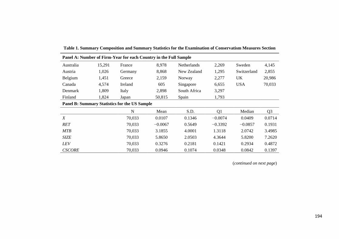
194
Table 1. Summary Composition and Summary Statistics for the Examination of Conservatism Measures Section
Panel A: Number of Firm-Year for each Country in the Full Sample
Australia 15,291 France 8,978 Netherlands 2,269 Sweden 4,145
Austria 1,026 Germany 8,868 New Zealand 1,295 Switzerland 2,855
Belgium 1,451 Greece 2,159 Norway 2,277 UK 20,986
Canada 4,574 Ireland 605 Singapore 6,655 USA 70,033
Denmark 1,809 Italy 2,898 South Africa 3,297
Finland 1,824 Japan 50,815 Spain 1,793
Panel B: Summary Statistics for the US Sample
N Mean S.D. Q1 Median Q3
X 70,033 0.0107 0.1346 −0.0074 0.0409 0.0714
RET 70,033 −0.0067 0.5649 −0.3392 −0.0857 0.1931
MTB 70,033 3.1855 4.0001 1.3118 2.0742 3.4985
SIZE 70,033 5.8650 2.0503 4.3644 5.8200 7.2620
LEV 70,033 0.3276 0.2181 0.1421 0.2934 0.4872
CSCORE 70,033 0.0946 0.1074 0.0348 0.0842 0.1397
(continued on next page)

195
Table 1. (continued)
Panel C: Summary Statistics for the Full Sample
N Mean S.D. Q1 Median Q3
X 215,903 0.0123 0.2822 −0.0105 0.0406 0.0792
RET 215,903 0.0004 0.4450 −0.2497 −0.0105 0.2276
MTB 215,903 2.4499 3.2104 0.8991 1.5506 2.7089
SIZE 215,903 6.4456 2.9050 4.1851 6.1918 8.5714
LEV 215,903 0.4129 0.2451 0.2068 0.4009 0.6046
CSCORE 215,903 0.0569 0.1320 −0.0194 0.0553 0.1271
Panel A of Table 1 reports the number of firm-year observations for each country in the final sample. Panels B and C of Table 1
report summary statistics for the variables used in hypotheses H1-H5 for the US and the full samples, respectively. X and RET are
trimmed at the top and bottom 1%. MTB, SIZE and LEV are winsorized at the top and bottom 1%. All variables are defined in
Appendix A.

196
Table 2. The Unconditional Association between AT and VR
US Sample Full Sample
AT Decile VR AT VR AT
1 1.1724 0.0137 1.2247 −0.0187
2 1.2289 0.0847 1.1734 0.0495
3 1.1744 0.1102 1.4303 0.0734
4 1.7283 0.1321 1.3889 0.1049
5 1.4783 0.1571 1.4023 0.1343
6 1.5774 0.1842 1.3040 0.1663
7 2.8953 0.2135 1.7732 0.2007
8 2.5770 0.2484 1.8199 0.2423
9 3.1620 0.3146 1.8303 0.3112
10 2.1389 0.4363 1.8938 1.2566
Table 2 reports pooled cross-sectional values of AT and VR across AT deciles for the US and the full samples. AT and VR are
calculated for each industry-year using the Fama and French 12-industry classification, excluding financial firms, between
1990 and 2015. The industry-year values of AT are sorted into deciles and then the corresponding VR value is calculated for
each AT decile. All variables are defined in Appendix A.
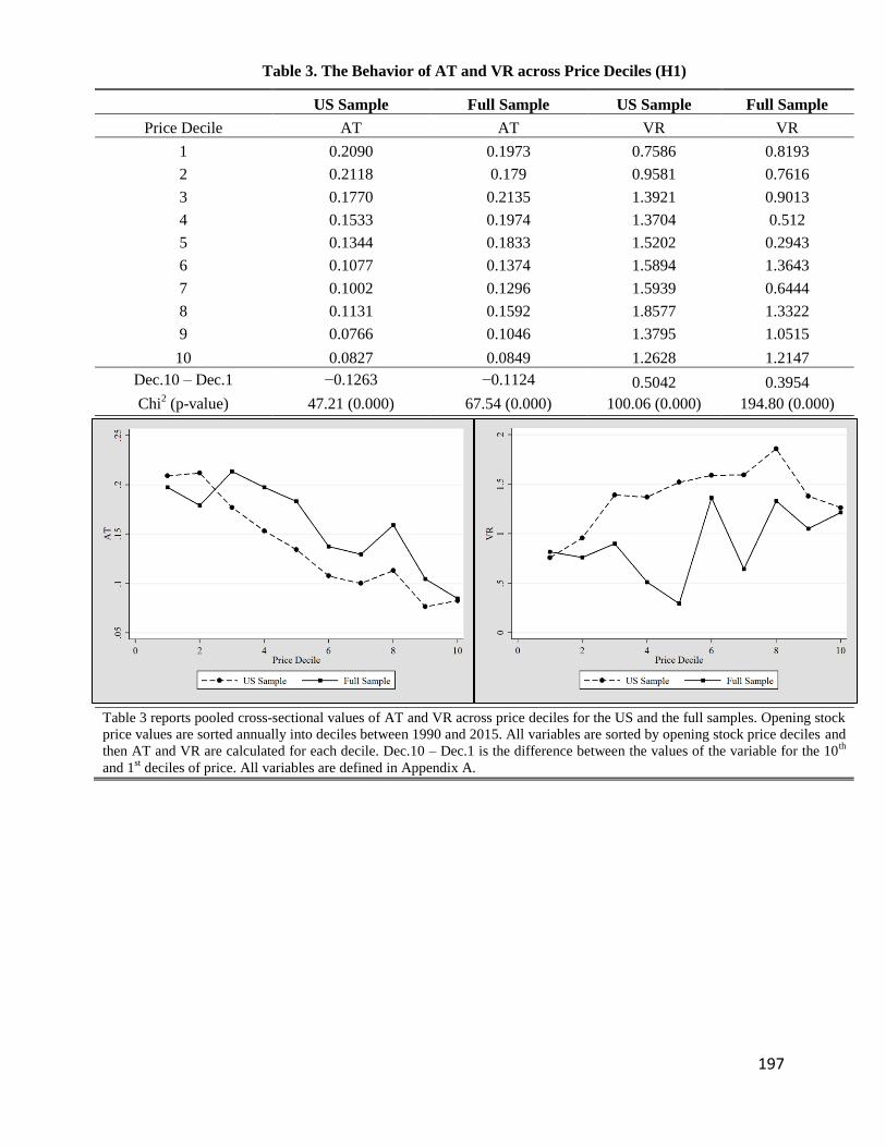
197
Table 3. The Behavior of AT and VR across Price Deciles (H1)
US Sample Full Sample US Sample Full Sample
Price Decile AT AT VR VR
1 0.2090 0.1973 0.7586 0.8193
2 0.2118 0.179 0.9581 0.7616
3 0.1770 0.2135 1.3921 0.9013
4 0.1533 0.1974 1.3704 0.512
5 0.1344 0.1833 1.5202 0.2943
6 0.1077 0.1374 1.5894 1.3643
7 0.1002 0.1296 1.5939 0.6444
8 0.1131 0.1592 1.8577 1.3322
9 0.0766 0.1046 1.3795 1.0515
10 0.0827 0.0849 1.2628 1.2147
Dec.10 – Dec.1 −0.1263 −0.1124 0.5042 0.3954
Chi2 (p-value) 47.21 (0.000) 67.54 (0.000) 100.06 (0.000) 194.80 (0.000)
Table 3 reports pooled cross-sectional values of AT and VR across price deciles for the US and the full samples. Opening stock
price values are sorted annually into deciles between 1990 and 2015. All variables are sorted by opening stock price deciles and
then AT and VR are calculated for each decile. Dec.10 – Dec.1 is the difference between the values of the variable for the 10th
and 1st deciles of price. All variables are defined in Appendix A.

198
Table 4. The Behavior of AT and VR across MTB Deciles (H2)
US Sample Full Sample US Sample Full Sample
MTB Decile AT AT VR VR
1 0.4309 0.4990 0.9403 0.8473
2 0.2813 0.3778 1.3595 1.5902
3 0.2713 0.3213 1.7630 1.6932
4 0.2210 0.2517 1.3351 1.5711
5 0.1670 0.2379 1.5568 1.6721
6 0.1601 0.1958 1.1210 0.5558
7 0.1440 0.1680 1.2502 0.9618
8 0.1257 0.1383 1.0610 1.2157
9 0.1105 0.1317 0.9039 1.0533
10 0.0788 0.0879 0.8503 0.8630
Dec.10 – Dec.1 −0.3521 −0.4111 −0.0900 0.0157
Chi2 (p-value) 215.14 (0.000) 163.14 (0.000) 4.33 (0.037) 0.44 (0.504)
Table 4 reports pooled cross-sectional values of AT and VR across MTB deciles for the US and the full samples. Opening MTB
values are sorted annually into deciles between 1990 and 2015. All variables are sorted by opening MTB deciles and then AT
and VR are calculated for each decile. Dec.10 – Dec.1 is the difference between the values of the variable for the 10th
and 1st
deciles of MTB. All variables are defined in Appendix A.

199
Table 5. The Behavior of AT and VR across SIZE Deciles (H3)
US Sample Full Sample US Sample Full Sample
SIZE Decile AT AT VR VR
1 0.2429 0.2116 0.7567 0.8795
2 0.2350 0.2068 1.0715 0.6700
3 0.1912 0.2249 1.1877 1.6717
4 0.1917 0.1935 1.3474 0.6334
5 0.1620 0.1573 1.1904 0.4786
6 0.1273 0.1384 1.3026 0.2994
7 0.1041 0.1474 1.5989 0.4232
8 0.1075 0.1162 1.3701 2.2036
9 0.1165 0.0918 2.0371 0.4302
10 0.1063 0.0694 1.5212 1.0588
Dec.10 – Dec.1 −0.1366 −0.1422 0.7645 0.1793
Chi2 (p-value) 52.65 (0.000) 80.86 (0.000) 171.88 (0.000) 45.50 (0.000)
Table 5 reports pooled cross-sectional values of AT and VR across SIZE deciles for the US and the full samples. Opening SIZE
values are sorted annually into deciles between 1990 and 2015. All variables are sorted by opening SIZE deciles and then AT
and VR are calculated for each decile. Dec.10 – Dec.1 is the difference between the values of the variable for the 10th
and 1st
deciles of SIZE. All variables are defined in Appendix A.
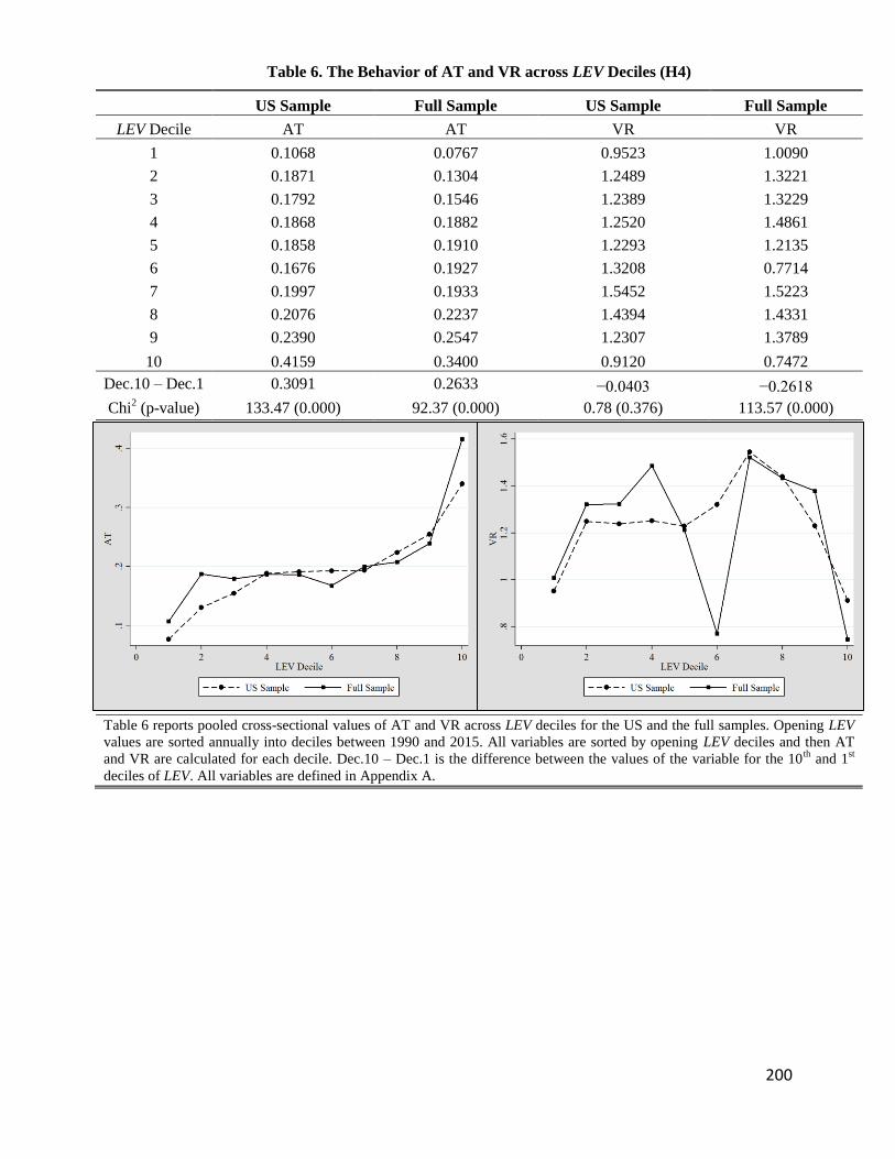
200
Table 6. The Behavior of AT and VR across LEV Deciles (H4)
US Sample Full Sample US Sample Full Sample
LEV Decile AT AT VR VR
1 0.1068 0.0767 0.9523 1.0090
2 0.1871 0.1304 1.2489 1.3221
3 0.1792 0.1546 1.2389 1.3229
4 0.1868 0.1882 1.2520 1.4861
5 0.1858 0.1910 1.2293 1.2135
6 0.1676 0.1927 1.3208 0.7714
7 0.1997 0.1933 1.5452 1.5223
8 0.2076 0.2237 1.4394 1.4331
9 0.2390 0.2547 1.2307 1.3789
10 0.4159 0.3400 0.9120 0.7472
Dec.10 – Dec.1 0.3091 0.2633 −0.0403 −0.2618
Chi2 (p-value) 133.47 (0.000) 92.37 (0.000) 0.78 (0.376) 113.57 (0.000)
Table 6 reports pooled cross-sectional values of AT and VR across LEV deciles for the US and the full samples. Opening LEV
values are sorted annually into deciles between 1990 and 2015. All variables are sorted by opening LEV deciles and then AT
and VR are calculated for each decile. Dec.10 – Dec.1 is the difference between the values of the variable for the 10th
and 1st
deciles of LEV. All variables are defined in Appendix A.
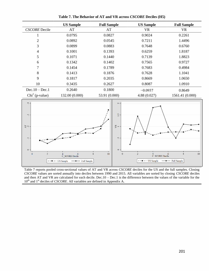
201
Table 7. The Behavior of AT and VR across CSCORE Deciles (H5)
US Sample Full Sample US Sample Full Sample
CSCORE Decile AT AT VR VR
1 0.0795 0.0827 0.9024 0.2261
2 0.0892 0.0545 0.7211 1.4496
3 0.0899 0.0883 0.7648 0.6760
4 0.1001 0.1393 0.6259 1.8187
5 0.1071 0.1440 0.7139 1.8823
6 0.1342 0.1402 0.7565 0.9727
7 0.1454 0.1789 0.7683 0.4984
8 0.1413 0.1876 0.7628 1.1041
9 0.1817 0.2035 0.8669 1.0650
10 0.3435 0.2627 0.8087 1.0910
Dec.10 – Dec.1 0.2640 0.1800 −0.0937 0.8649
Chi2 (p-value) 132.00 (0.000) 53.91 (0.000) 4.88 (0.027) 1561.41 (0.000)
Table 7 reports pooled cross-sectional values of AT and VR across CSCORE deciles for the US and the full samples. Closing
CSCORE values are sorted annually into deciles between 1990 and 2015. All variables are sorted by closing CSCORE deciles
and then AT and VR are calculated for each decile. Dec.10 – Dec.1 is the difference between the values of the variable for the
10th
and 1st deciles of CSCORE. All variables are defined in Appendix A.
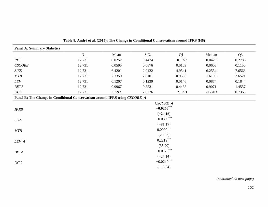
202
Table 8. André et al. (2015): The Change in Conditional Conservatism around IFRS (H6)
Panel A: Summary Statistics
N Mean S.D. Q1 Median Q3
RET 12,731 0.0252 0.4474 −0.1925 0.0429 0.2786
CSCORE 12,731 0.0595 0.0876 0.0109 0.0606 0.1150
SIZE 12,731 6.4201 2.0122 4.9541 6.2554 7.6563
MTB 12,731 2.3350 2.8101 0.9536 1.6106 2.6521
LEV 12,731 0.1207 0.1239 0.0146 0.0874 0.1844
BETA 12,731 0.9967 0.8531 0.4488 0.9071 1.4557
UCC 12,731 −0.5921 2.6226 −2.1991 -0.7703 0.7368
Panel B: The Change in Conditional Conservatism around IFRS using CSCORE_A
CSCORE_A
IFRS −0.0256***
(−24.16)
SIZE −0.0300***
(−81.17)
MTB 0.0090***
(25.03)
LEV_A 0.2219***
(35.20)
BETA −0.0175***
(−24.14)
UCC −0.0249***
(−73.04)
(continued on next page)
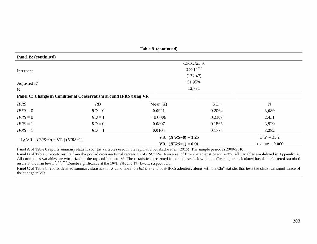
203
Table 8. (continued)
Panel B: (continued)
CSCORE_A
Intercept 0.2211***
(132.47)
Adjusted R2 51.95%
N 12,731
Panel C: Change in Conditional Conservatism around IFRS using VR
IFRS RD Mean (X) S.D. N
IFRS = 0 RD = 0 0.0921 0.2064 3,089
IFRS = 0 RD = 1 −0.0006 0.2309 2,431
IFRS = 1 RD = 0 0.0897 0.1866 3,929
IFRS = 1 RD = 1 0.0104 0.1774 3,282
H0: VR | (IFRS=0) = VR | (IFRS=1) VR | (IFRS=0) = 1.25 Chi
2 = 35.2
VR | (IFRS=1) = 0.91 p-value = 0.000
Panel A of Table 8 reports summary statistics for the variables used in the replication of Andre et al. (2015). The sample period is 2000-2010.
Panel B of Table 8 reports results from the pooled cross-sectional regression of CSCORE_A on a set of firm characteristics and IFRS. All variables are defined in Appendix A.
All continuous variables are winsorized at the top and bottom 1%. The t-statistics, presented in parentheses below the coefficients, are calculated based on clustered standard
errors at the firm level. *,
**,
*** Denote significance at the 10%, 5%, and 1% levels, respectively.
Panel C of Table 8 reports detailed summary statistics for X conditional on RD pre- and post-IFRS adoption, along with the Chi2 statistic that tests the statistical significance of
the change in VR.
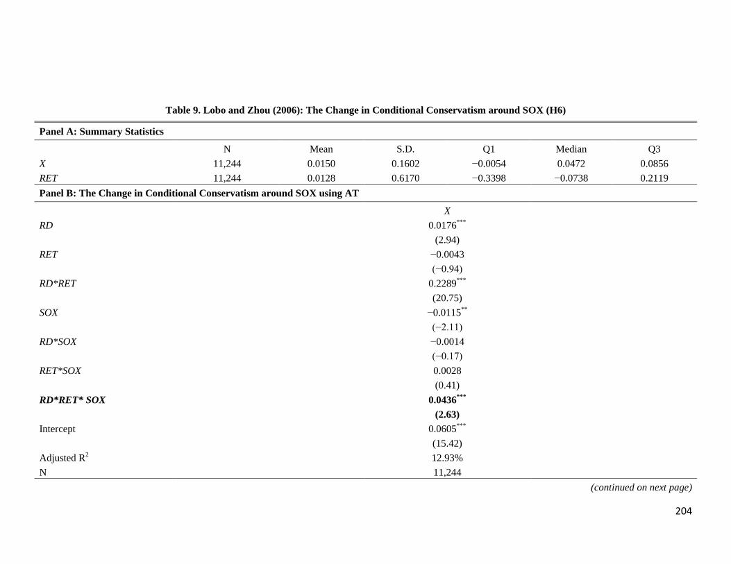
204
Table 9. Lobo and Zhou (2006): The Change in Conditional Conservatism around SOX (H6)
Panel A: Summary Statistics
N Mean S.D. Q1 Median Q3
X 11,244 0.0150 0.1602 −0.0054 0.0472 0.0856
RET 11,244 0.0128 0.6170 −0.3398 −0.0738 0.2119
Panel B: The Change in Conditional Conservatism around SOX using AT
X
RD 0.0176***
(2.94)
RET −0.0043
(−0.94)
RD*RET 0.2289***
(20.75)
SOX −0.0115**
(−2.11)
RD*SOX −0.0014
(−0.17)
RET*SOX 0.0028
(0.41)
RD*RET* SOX 0.0436***
(2.63)
Intercept 0.0605***
(15.42)
Adjusted R2 12.93%
N 11,244
(continued on next page)
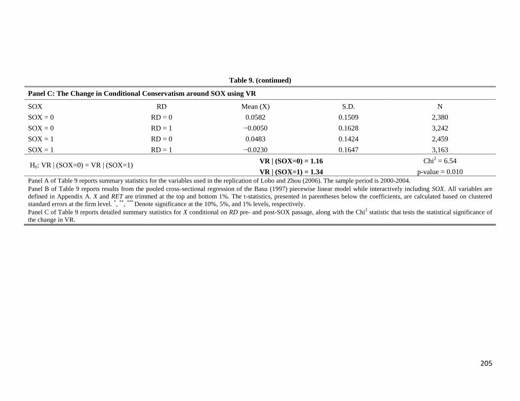
205
Table 9. (continued)
Panel C: The Change in Conditional Conservatism around SOX using VR
SOX RD Mean (X) S.D. N
SOX = 0 RD = 0 0.0582 0.1509 2,380
SOX = 0 RD = 1 −0.0050 0.1628 3,242
SOX = 1 RD = 0 0.0483 0.1424 2,459
SOX = 1 RD = 1 −0.0230 0.1647 3,163
H0: VR | (SOX=0) = VR | (SOX=1) VR | (SOX=0) = 1.16 Chi
2 = 6.54
VR | (SOX=1) = 1.34 p-value = 0.010
Panel A of Table 9 reports summary statistics for the variables used in the replication of Lobo and Zhou (2006). The sample period is 2000-2004.
Panel B of Table 9 reports results from the pooled cross-sectional regression of the Basu (1997) piecewise linear model while interactively including SOX. All variables are
defined in Appendix A. X and RET are trimmed at the top and bottom 1%. The t-statistics, presented in parentheses below the coefficients, are calculated based on clustered
standard errors at the firm level. *,
**,
*** Denote significance at the 10%, 5%, and 1% levels, respectively.
Panel C of Table 9 reports detailed summary statistics for X conditional on RD pre- and post-SOX passage, along with the Chi2 statistic that tests the statistical significance of
the change in VR.

206
Table 10. Ball et al. (2008): The Effect of Debt and Equity Markets in Shaping Financial Reporting (H7a)
Panel A: Summary Statistics
N Mean S.D. Q1 Median Q3
X 96,379 −0.0071 0.2625 −0.0093 0.0321 0.0728
RET 96,379 −0.0076 0.5528 −0.3023 −0.0282 0.2327
Panel B: Extract from the Full Dataset Used to Replicate Ball et al. (2008)
Country B0 B1 B2 B3 VR DEBT EQUITY LAW CORRUPT CREDIT BTM
Australia 0.017 −0.027 0.004 0.272 1.90 0.76 0.49 10.00 8.52 1 0.638
Canada 0.051 0.002 −0.001 0.293 1.64 0.72 0.39 10.00 10.00 1 0.682
Malaysia −0.012 −0.010 −0.023 0.160 1.19 0.84 1.48 6.78 7.38 4 0.789
Singapore 0.016 0.004 0.087 0.013 1.00 0.60 1.18 8.57 8.22 3 0.817
South Africa 0.101 −0.001 0.147 −0.017 0.70 0.93 1.45 4.42 8.92 4 0.738
Thailand 0.030 −0.016 0.003 0.365 0.86 0.93 0.56 6.25 5.18 3 0.944
UK 0.041 −0.018 −0.026 0.193 1.48 1.13 1.00 8.57 9.10 4 0.514
USA 0.035 0.012 −0.026 0.228 1.51 0.81 0.58 10.00 8.63 1 0.475
Brazil 0.043 −0.061 −0.019 0.027 0.61 0.39 0.18 6.32 6.32 1 0.004
Chile 0.061 0.002 0.098 0.116 1.29 0.63 0.80 7.02 5.30 2 0.815
France 0.043 −0.007 0.022 0.216 2.33 0.96 0.23 8.98 9.05 0 0.702
Indonesia −0.021 −0.006 0.045 −0.025 1.09 0.42 0.15 3.98 2.15 4 0.775
Italy 0.054 0.000 −0.019 0.129 1.04 0.55 0.08 8.33 6.13 2 1.052
Netherlands 0.079 −0.005 −0.036 0.221 1.82 1.08 0.52 10.00 10.00 2 0.566
Spain 0.119 −0.018 −0.046 0.132 0.61 0.75 0.17 7.80 7.38 2 0.787
Germany 0.012 −0.039 0.023 0.212 1.72 1.12 0.13 9.23 8.93 3 0.628
Japan 0.009 −0.010 0.045 0.081 2.00 1.22 0.62 8.98 8.52 2 0.793
(continued on next page)

207
Table 10. (continued)
Panel B: (continued)
Country B0 B1 B2 B3 VR DEBT EQUITY LAW CORRUPT CREDIT BTM
South Korea 0.056 −0.039 0.239 0.032 1.25 0.74 0.44 5.35 5.30 3 1.810
Denmark 0.088 −0.028 0.048 0.127 1.36 0.34 0.21 10.00 10.00 3 0.848
Finland 0.093 −0.024 0.075 0.071 0.78 0.75 0.25 10.00 10.00 1 0.811
Norway 0.052 −0.011 −0.016 0.230 1.81 0.64 0.22 10.00 10.00 2 0.650
Sweden 0.022 0.011 0.078 0.270 4.16 0.55 0.51 10.00 10.00 2 0.657
Mean 0.045 −0.013 0.032 0.152 1.462 0.766 0.529 8.208 7.956 2.273 0.750
Median 0.043 −0.010 0.013 0.146 1.325 0.750 0.465 8.775 8.575 2.000 0.757
S.D. 0.036 0.018 0.069 0.108 0.770 0.245 0.416 1.947 2.102 1.162 0.313
Panel A of Table 10 reports summary statistics for the variables used in replicating Ball et al. (2008). The sample period is 1992-
2003.
Panel B of Table 10 reports the estimates obtained from the Basu (1997) pooled cross-sectional regression in each country, the
VR value for each country and a set of country-level variables. X and RET are trimmed at the top and bottom 1%. All variables
are defined in Appendix A.

208
Table 11. The Effect of Debt and Equity Markets on Conditional Conservatism using AT (H7a)
B3 B3 B3 B3 B3 B3 B3 B3 B3
DEBT 0.2656**
0.1987* 0.2592
* 0.2518
** 0.2550
** 0.1978
* 0.2686
* 0.2568
** 0.2569
*
(2.81) (1.87) (2.13) (2.53) (2.25) (1.80) (2.14) (2.16) (2.08)
EQUITY −0.1875***
−0.1472**
−0.1869***
−0.1661**
−0.1174 −0.1501* −0.1626
* −0.1145 −0.117
(−3.08) (−2.18) (−2.96) (−2.29) (−1.67) (−2.05) (−2.13) (−1.47) (−1.44)
ENGLISH 0.2223***
0.1863**
0.2200**
0.2087**
0.1939**
0.1874**
0.2125**
0.1931**
0.2010**
(3.27) (2.58) (2.94) (2.84) (2.72) (2.49) (2.74) (2.60) (2.44)
FRENCH 0.0823 0.0689 0.0813 0.0702 0.0745 0.0712 0.0703 0.0727 0.0823
(1.25) (1.05) (1.18) (0.99) (1.16) (1.02) (0.96) (1.05) (1.03)
SCAND 0.1688**
0.1071 0.163 0.1569* 0.1564 0.106 0.1722 0.1582 0.1614
(2.20) (1.20) (1.58) (1.93) (1.63) (1.14) (1.62) (1.57) (1.53)
LAW
0.0163
0.0331* 0.0175
0.0325 0.0323
(1.29)
(1.82) (1.11)
(1.63) (1.57)
CORRUPT
0.0012
−0.0234
−0.0038 −0.0238 −0.0223
(0.09)
(−1.26)
(−0.23) (−1.21) (−1.05)
CREDIT
−0.0115
0.0031 −0.0144 −0.0025 −0.0026
(−0.58)
(0.13) (−0.60) (−0.10) (−0.10)
BTM
0.0206
(0.27)
Intercept −0.09 −0.1657 −0.0928 −0.0537 −0.1894 −0.1807 −0.0358 −0.1776 −0.2095
(−0.84) (−1.38) (−0.81) (−0.42) (−1.58) (−1.06) (−0.24) (−1.06) (−1.00)
(continued on next page)

209
Table 11. (continued)
B3 B3 B3 B3 B3 B3 B3 B3 B3
Adjusted R2 53.77% 58.35% 53.79% 54.77% 62.59% 58.40% 54.94% 62.63% 62.86%
N 22 22 22 22 22 22 22 22 22
Table 11 reports pooled cross-sectional regression results that use the AT coefficient estimates (B3) reported in Table 10 in order
to replicate Ball et al. (2008). All variables are defined in Appendix A. The t-statistics, presented in parentheses below the
coefficients, are calculated based on White (1980) standard errors. *,
**,
*** Denote significance at the 10%, 5%, and 1% levels,
respectively.

210
Table 12. The Effect of Debt and Equity Markets on Conditional Conservatism using VR (H7a)
VR VR VR VR VR VR VR VR VR
DEBT 0.9134 0.1215 0.3079 0.6631 0.2778 0.1423 0.4169 0.3372 0.336
(1.03) (0.13) (0.28) (0.74) (0.26) (0.14) (0.37) (0.30) (0.29)
EQUITY −0.0393 0.4385 0.0175 0.3491 0.521 0.5033 0.2981 0.6208 0.6427
(−0.07) (0.72) (0.03) (0.53) (0.78) (0.76) (0.43) (0.85) (0.84)
ENGLISH −0.1817 −0.6085 −0.3978 −0.4292 −0.5874 −0.634 −0.485 −0.6154 −0.6876
(−0.29) (−0.93) (−0.58) (−0.65) (−0.87) (−0.93) (−0.69) (−0.88) (−0.88)
FRENCH −0.0905 −0.2484 −0.1839 −0.3093 −0.2328 −0.2992 −0.3107 −0.2942 −0.3811
(−0.15) (−0.42) (−0.29) (−0.48) (−0.38) (−0.47) (−0.47) (−0.45) (−0.51)
SCAND 0.7841 0.0544 0.2388 0.5694 0.1912 0.0788 0.3455 0.2511 0.2218
(1.09) (0.07) (0.26) (0.78) (0.21) (0.09) (0.36) (0.26) (0.22)
LAW
0.1935
0.2401 0.1685
0.2181 0.2197
(1.68)
(1.39) (1.18)
(1.16) (1.13)
CORRUPT
0.1135
−0.065
0.0557 −0.0788 −0.0931
(0.91)
(−0.37)
(0.38) (−0.42) (−0.47)
CREDIT
−0.2082
−0.0678 −0.166 −0.0862 −0.0858
(−1.15)
(−0.32) (−0.77) (−0.38) (−0.37)
BTM
−0.1863
(−0.26)
Intercept 0.7345 −0.1616 0.4726 1.3927 −0.2273 0.1684 1.1307 0.1786 0.4673
(0.73) (−0.15) (0.45) (1.22) (−0.20) (0.11) (0.83) (0.11) (0.24)
(continued on next page)
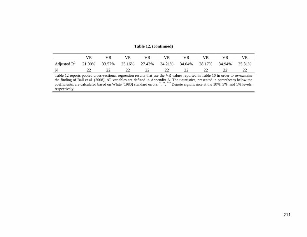
211
Table 12. (continued)
VR VR VR VR VR VR VR VR VR
Adjusted R2 21.00% 33.57% 25.16% 27.43% 34.21% 34.04% 28.17% 34.94% 35.31%
N 22 22 22 22 22 22 22 22 22
Table 12 reports pooled cross-sectional regression results that use the VR values reported in Table 10 in order to re-examine
the finding of Ball et al. (2008). All variables are defined in Appendix A. The t-statistics, presented in parentheses below the
coefficients, are calculated based on White (1980) standard errors. *,
**,
*** Denote significance at the 10%, 5%, and 1% levels,
respectively.
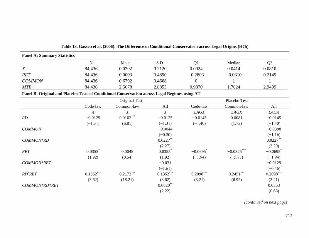
212
Table 13. Gassen et al. (2006): The Difference in Conditional Conservatism across Legal Origins (H7b)
Panel A: Summary Statistics
N Mean S.D. Q1 Median Q3
X 84,436 0.0202 0.2120 0.0024 0.0414 0.0810
RET 84,436 0.0003 0.4890 −0.2803 −0.0310 0.2149
COMMON 84,436 0.6792 0.4668 0 1 1
MTB 84,436 2.5678 2.8855 0.9870 1.7024 2.9499
Panel B: Original and Placebo Tests of Conditional Conservatism across Legal Regimes using AT
Original Test Placebo Test
Code-law Common-law All Code-law Common-law All
X X X LAGX LAGX LAGX
RD −0.0125 0.0102***
−0.0125 −0.0145 0.0081 −0.0145
(−1.31) (6.81) (−1.31) (−1.40) (1.73) (−1.40)
COMMON −0.0044 −0.0388
(−0.20) (−1.16)
COMMON*RD 0.0227**
0.0227**
(2.27) (2.20)
RET 0.0355* 0.0045 0.0355
* −0.0695
* −0.0825
*** −0.0695
*
(1.92) (0.54) (1.92) (−1.94) (−5.77) (−1.94)
COMMON*RET −0.031 −0.0129
(−1.61) (−0.46)
RD*RET 0.1352
*** 0.2172
*** 0.1352
*** 0.2098
*** 0.2451
*** 0.2098
***
(3.62) (18.21) (3.62) (3.21) (6.92) (3.21)
COMMON*RD*RET 0.0820**
0.0353
(2.22) (0.63)
(continued on next page)
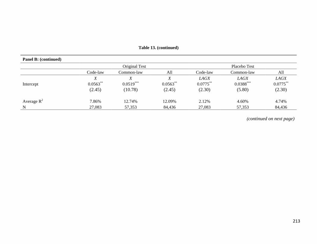
213
Table 13. (continued)
Panel B: (continued)
Original Test Placebo Test
Code-law Common-law All Code-law Common-law All
X X X LAGX LAGX LAGX
Intercept 0.0563**
0.0519***
0.0563**
0.0775**
0.0388***
0.0775**
(2.45) (10.78) (2.45) (2.30) (5.80) (2.30)
Average R2 7.86% 12.74% 12.09% 2.12% 4.60% 4.74%
N 27,083 57,353 84,436 27,083 57,353 84,436
(continued on next page)

214
Table 13. (Continued)
Panel C: Original and Placebo Tests of Conditional Conservatism across Legal Regimes using VR
Original Test Placebo Test
Code-law Sample Code-law Sample
RD Mean(X) S.D. N RD Mean (LAGX) S.D. N
RD = 0 0.0680 0.2560 13,790 RD = 0 0.0687 0.4527 13,790
RD = 1 −0.0004 0.2671 13,293 RD = 1 0.0307 0.4400 13,293
VR = 1.09
VR = 0.94
H0: VR = 1 F-stat (p-value): 22.91 (0.000) H0: VR = 1 F-stat (p-value): 3.31 (0.068)
Common-law Sample Common-law Sample
RD Mean(X) S.D. N RD Mean (LAGX) S.D. N
RD = 0 0.0508 0.1695 25,475 RD = 0 −0.0014 0.2637 25,475
RD = 1 −0.0164 0.1864 31,878 RD = 1 −0.0134 0.2494 31,878
VR = 1.21
VR = 0.89
H0: VR = 1 F-stat (p-value): 287.91 (0.000) H0: VR = 1 F-stat (p-value): 7.86 (0.005)
Panel A of Table 13 reports summary statistics for the variables used in the replication of Gassen et al. (2006). The sample period is 1990-2003.
Panel B of Table 13 reports results from the annual cross-sectional regressions of the Basu (1997) model while interactively including COMMON. The first three
columns are the original test where the dependent variable is X while the last three columns are the placebo test where the dependent variable is LAGX. All variables
are defined in Appendix A. X, RET and LAGX are winsorized at the upper and bottom 1%. The t-statistics, presented in parentheses below the coefficients, are
calculated based on Fama-MacBeth standard errors. *,
**,
*** Denote significance at the 10%, 5%, and 1% levels, respectively.
Panel C of Table 13 reports detailed summary statistics for X and LAGX conditional on RD, for Common-law and Code-law samples, from the original and the
placebo tests. The reported F-statistics test the significance of the null hypothesis that VR equals 1.

215
Table 14. Gassen et al. (2006): The Difference in Conditional Conservatism across MTB Deciles (H7a)
Panel A: The Change in AT across MTB Deciles
Code-law Common-law All
X X X
RD −0.0328* −0.0008 −0.0185
(−1.89) (−0.13) (−1.65)
RMTB −0.0118 0.0007 −0.0053
(−1.47) (0.45) (−1.14)
RMTB*RD 0.0053**
0.0017* 0.0035
**
(2.32) (1.77) (2.41)
RET 0.0221 0.0325**
0.0135
(0.71) (2.34) (0.68)
RMTB*RET 0.0042 −0.0050***
−0.0012
(0.98) (−3.99) (−0.52)
RD*RET 0.3272***
0.3579***
0.3853***
(4.04) (13.43) (7.22)
RMTB*RD*RET −0.0355***
−0.0232***
−0.0312***
(−3.17) (−7.47) (−4.56)
Intercept 0.1104* 0.0482
*** 0.0851
**
(2.01) (3.72) (2.43)
Average R2 12.88% 17.13% 15.35%
N 27,083 57,353 84,436
(continued on next page)

216
Panel B: The Behavior of Conditional Conservatism across MTB Deciles using AT and VR
MTB Decile AT VR
1 0.417 1.06
2 0.307 1.44
3 0.248 1.93
4 0.212 1.82
5 0.196 1.68
6 0.162 1.29
7 0.131 1.84
8 0.130 1.32
9 0.113 1.25
10 0.101 0.97
Dec.10 – Dec.1 −0.308 −0.09
Chi2 (p-value) 144.93 (0.000) 3.94 (0.047)
Panel A of Table 14 reports results from the annual cross-sectional regressions of the Basu (1997) model while interactively including RMTB. All variables are defined in
Appendix A. X and RET are winsorized at the top and bottom 1%. The t-statistics, presented in parentheses below the coefficients, are calculated based on Fama-MacBeth
standard errors. *,
**,
*** Denote significance at the 10%, 5%, and 1% levels, respectively.
Panel B of Table 13 reports the mean values of AT and VR across MTB deciles for the full sample. Dec.10 – Dec.1 is the difference between the values of the variable for the
10th
and 1st deciles of MTB.
217
Chapter 5
Summary and Suggestions for Future Research
This thesis examines the interaction between financial reporting and information
asymmetry in relation to their effect on the behavior of market participants. I first assess
the impact of changes in accounting standards on corporate payout and equity financing
choices. The overall inference is that imposing higher quality financial reporting standards
serves to mitigate information asymmetry and, accordingly, reduce frictions affecting
corporate financial decisions. I then evaluate the empirical measurement of conditional
conservatism, a feature of financial reporting meant to mitigate information asymmetry.
My findings imply that the literature has drawn several conclusions about the role of
accounting conservatism in capital markets based on a biased measure of conditional
conservatism. Accordingly, a considerable number of prior studies need to be revisited in
light of a more appropriate measure of conditional conservatism.
Chapter 2 examines the change in dividend payout policy and dividend value relevance
following the mandatory adoption of IFRS. The first main hypothesis is based on prior
findings that the mandatory adoption of IFRS serves to mitigate information asymmetry,
due to better accounting quality and increased financial disclosure, and accordingly eases
external financing. As a result, managers are expected to retain less cash and pay more
dividends to shareholders since raising external funds becomes less costly. Concurrently,
the other main hypothesis predicts that improving accounting standards increases
accounting value relevance and decreases dividend value relevance. That is, investors are
expected to have more confidence in accounting numbers and, thus, dividends would lose
from their signaling power. The empirical findings confirm the aforementioned
hypotheses.
Chapter 3 examines whether imposing higher quality accounting standards serves to
mitigate earnings management activities in situations where such activities are found to be

218
high. In particular, the first hypothesis examines the change in the level of earnings
management prior to issuing new equity following the mandatory adoption of IFRS. The
reduction in earnings management and information asymmetry following the IFRS
mandate is expected to improve the market reaction to SEOs, which is the second
hypothesis. Accordingly, an improved market reaction to equity offerings implies a
reduction in the costs associated with equity financing. Therefore, the final hypothesis
predicts that the propensity to issue new equity would increase following IFRS adoption.
The reported results indicate that the formulated hypotheses are in the right direction.
Extending Chapters 2 and 3 would include the addition of more countries to the sample
in order to generalize the findings. A bigger sample would also allow for a tighter
matching based on several firm-level variables that might drive the results in the current
chapters, such as corporate governance and underlying economic characteristics. However,
this would come at the cost of compromising the high comparability between the control
and treatment groups in my study, that is, the UK and France. This is because the effect of
IFRS adoption is determined to a large extent by several country characteristics that drive
the effect of IFRS per se. A plausible solution might be the addition of some country-level
variables that control for variations in financial reporting incentives, enforcement changes,
institutional infrastructures, legal systems, and corruption.
Chapter 4 evaluates the empirical estimation of conditional conservatism in accounting
data. As mentioned in the introduction of the chapter, several important conclusions were
drawn about the role of accounting conservatism in capital markets based on the
asymmetric timeliness measures (i.e., the AT and the C_Score measures). Yet, recent
studies provide evidence showing a substantial upward bias in the original asymmetric
timeliness measure (i.e., the AT measure) arising from non-accounting (economic) factors.
Therefore, this chapter aims to evaluate prior studies in light of a new alternative measure
of conditional conservatism, the VR measure. The first part of the analysis shows that the
economic bias implicit in the AT measure also drives the C_Score measure; however, the

219
VR measure seems unaffected by this bias. The other part of the analysis replicates four
prior studies that use the AT measure (or the C_Score measure), and then re-examines the
replicated results using the VR measure. The findings show that the AT and the VR
measures yield similar conclusions when used to model the change in conditional
conservatism for the same sample following an exogenous change in accounting policy.
The intuition here is that the economic bias for the same group of firms is expected to
cancel out when the regression model measures the change in the AT coefficient estimate.
On the other hand, the AT and the VR measures yield inconsistent conclusions when used
to model the cross-sectional variation in conditional conservatism. This is attributed to the
different underlying economic characteristics across different cross-sections, which results
in a different magnitude of the AT bias between samples.
Chapter 4 opens the door to re-examining prior studies on conditional conservatism and
to reaching more reliable conclusions about the costs and benefits of conditional
conservatism. Despite the fact that I praise the VR measure in light of my findings, yet this
measure suffers from some limitations. Specifically, the VR measure cannot be estimated
at the firm-year level. This should motivate researchers to develop a new firm-year
measure in spirit of the VR measure in a similar way that the C_Score measure was
developed based on the AT measure. In addition, the VR measure is sensitive to outliers
and becomes more sensitive when estimating conditional conservatism for a small number
of observations. Thus, it might be helpful to check if the results hold after dropping the top
and bottom 5%, or perhaps 10%, of the main variable used in the VR measure (i.e.,
deflated earnings or deflated accruals).