Empirical Methods for Microeconomic Applications

University of Lugano, SwitzerlandMay 27-31, 2013

William Greene

Department of Economics

Stern School of Business

1C. Extensions of Binary Choice Models

Agenda for 1C• Endogenous RHS Variables• Sample Selection• Dynamic Binary Choice

Model• Bivariate Binary Choice• Simultaneous Equations• Ordered Choices

• Ordered Choice Model• Application to BHPS

Endogeneity

Endogenous RHS Variable

• U* = β’x + θh + εy = 1[U* > 0]

E[ε|h] ≠ 0 (h is endogenous)• Case 1: h is continuous• Case 2: h is binary, e.g., a treatment effect

• Approaches• Parametric: Maximum Likelihood• Semiparametric (not developed here):

GMM Various approaches for case 2

Endogenous Continuous Variable

U* = β’x + θh + εy = 1[U* > 0] h = α’z + u

E[ε|h] ≠ 0 Cov[u, ε] ≠ 0 Additional Assumptions:

(u,ε) ~ N[(0,0),(σu2, ρσu, 1)]

z = a valid set of exogenous variables, uncorrelated with (u,ε)

Correlation = ρ.This is the source of the endogeneity

Endogenous Income in Health

0 = Not Healthy 1 = Healthy

Healthy = 0 or 1

Age, Married, Kids, Gender, IncomeDeterminants of Income (observed and

unobserved) also determine health satisfaction.

Income responds to

Age, Age2, Educ, Married, Kids, Gender

Estimation by ML (Control Function)Probit fit of y to and will not consistently estimate ( , )

because of the correlation between h and induced by the

correlation of u and . Using the bivariate normality,

(Prob( 1| , )

h

hy h

x

xx

2

2

/ )

1

Insert = ( - )/ and include f(h| ) to form logL

-

log (2 1)1

logL=

- 1log

u

i i u

i ii i

ui

i i

u u

u

u h

hh

y

h

α z z

α zx

α z

N

i=1

Two Approaches to ML

u

(1) Maximize the full log likelihood

with respect to ( , , , , )

(The built in Stata routine IVPROBIT does this. It is not

an instrumental variable estimat

or; it i

Full information ML.

u

s a FIML estimator.)

(2)

(a) Use OLS to estimate and with and s.

ˆ ˆ (b) Compute = / = ( ) /

ˆ (c) log

i i i i

i i

v u s h s

h

Two step limited information ML. (Control Functio

a

a z

x

n)

2

ˆ ˆ ˆlog1

ˆThe second step is to fit a probit model for y to ( , , ) then

solve back for ( , , ) from ( , , ) and from the previously

estimated and s. Use the delta method to

ii i i

vh v

h v

x

x

a

compute standard errors.

FIML Estimates----------------------------------------------------------------------Probit with Endogenous RHS VariableDependent variable HEALTHYLog likelihood function -6464.60772--------+-------------------------------------------------------------Variable| Coefficient Standard Error b/St.Er. P[|Z|>z] Mean of X--------+------------------------------------------------------------- |Coefficients in Probit Equation for HEALTHYConstant| 1.21760*** .06359 19.149 .0000 AGE| -.02426*** .00081 -29.864 .0000 43.5257 MARRIED| -.02599 .02329 -1.116 .2644 .75862 HHKIDS| .06932*** .01890 3.668 .0002 .40273 FEMALE| -.14180*** .01583 -8.959 .0000 .47877 INCOME| .53778*** .14473 3.716 .0002 .35208 |Coefficients in Linear Regression for INCOMEConstant| -.36099*** .01704 -21.180 .0000 AGE| .02159*** .00083 26.062 .0000 43.5257 AGESQ| -.00025*** .944134D-05 -26.569 .0000 2022.86 EDUC| .02064*** .00039 52.729 .0000 11.3206 MARRIED| .07783*** .00259 30.080 .0000 .75862 HHKIDS| -.03564*** .00232 -15.332 .0000 .40273 FEMALE| .00413** .00203 2.033 .0420 .47877 |Standard Deviation of Regression DisturbancesSigma(w)| .16445*** .00026 644.874 .0000 |Correlation Between Probit and Regression DisturbancesRho(e,w)| -.02630 .02499 -1.052 .2926--------+-------------------------------------------------------------

Partial Effects: Scaled Coefficients

E[ | ] ( )

where ~ N[0,1]

E[y| , , ] = [ ( )]

=

E[y| , , ] [ ( )]( )

u

u

u

y h h

h u v v

v v

vv

Conditional Mean

x x

z z

x z x z

Partial Effects. Assume z x (just for convenience)

x zx z

x

,

R

1

E[y| , ] E[y| , , ] E ( ) [ ( )] ( )

E[y| , ] 1 . ( ) [ ( )]

v u

u rr

vv v dv

Est vR

x z x zx z

x x

The integral does not have a closed form, but it can easily be simulated :

x zx z

xFor v

k k , . , . ariables only in x omit For variables only in z omit

Endogenous Binary Variable

U* = β’x + θh + εy = 1[U* > 0]h* = α’z + uh = 1[h* > 0]

E[ε|h*] ≠ 0 Cov[u, ε] ≠ 0 Additional Assumptions: (u,ε) ~ N[(0,0),(σu

2, ρσu, 1)] z = a valid set of exogenous

variables, uncorrelated with (u,ε)

Correlation = ρ.This is the source of the endogeneity

Endogenous Binary VariableP(Y = y,H = h) = P(Y = y|H =h) x P(H=h)

This is a simple bivariate probit model.

Not a simultaneous equations model - the estimator

is FIML, not any kind of least squares.

Doctor = F(age,age2,income,female,Public) Public = F(age,educ,income,married,kids,female)

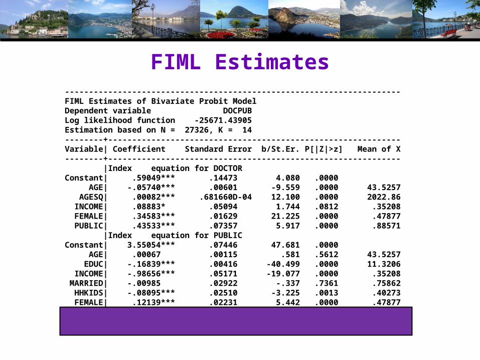
FIML Estimates----------------------------------------------------------------------FIML Estimates of Bivariate Probit ModelDependent variable DOCPUBLog likelihood function -25671.43905Estimation based on N = 27326, K = 14--------+-------------------------------------------------------------Variable| Coefficient Standard Error b/St.Er. P[|Z|>z] Mean of X--------+------------------------------------------------------------- |Index equation for DOCTORConstant| .59049*** .14473 4.080 .0000 AGE| -.05740*** .00601 -9.559 .0000 43.5257 AGESQ| .00082*** .681660D-04 12.100 .0000 2022.86 INCOME| .08883* .05094 1.744 .0812 .35208 FEMALE| .34583*** .01629 21.225 .0000 .47877 PUBLIC| .43533*** .07357 5.917 .0000 .88571 |Index equation for PUBLICConstant| 3.55054*** .07446 47.681 .0000 AGE| .00067 .00115 .581 .5612 43.5257 EDUC| -.16839*** .00416 -40.499 .0000 11.3206 INCOME| -.98656*** .05171 -19.077 .0000 .35208 MARRIED| -.00985 .02922 -.337 .7361 .75862 HHKIDS| -.08095*** .02510 -3.225 .0013 .40273 FEMALE| .12139*** .02231 5.442 .0000 .47877 |Disturbance correlationRHO(1,2)| -.17280*** .04074 -4.241 .0000--------+-------------------------------------------------------------

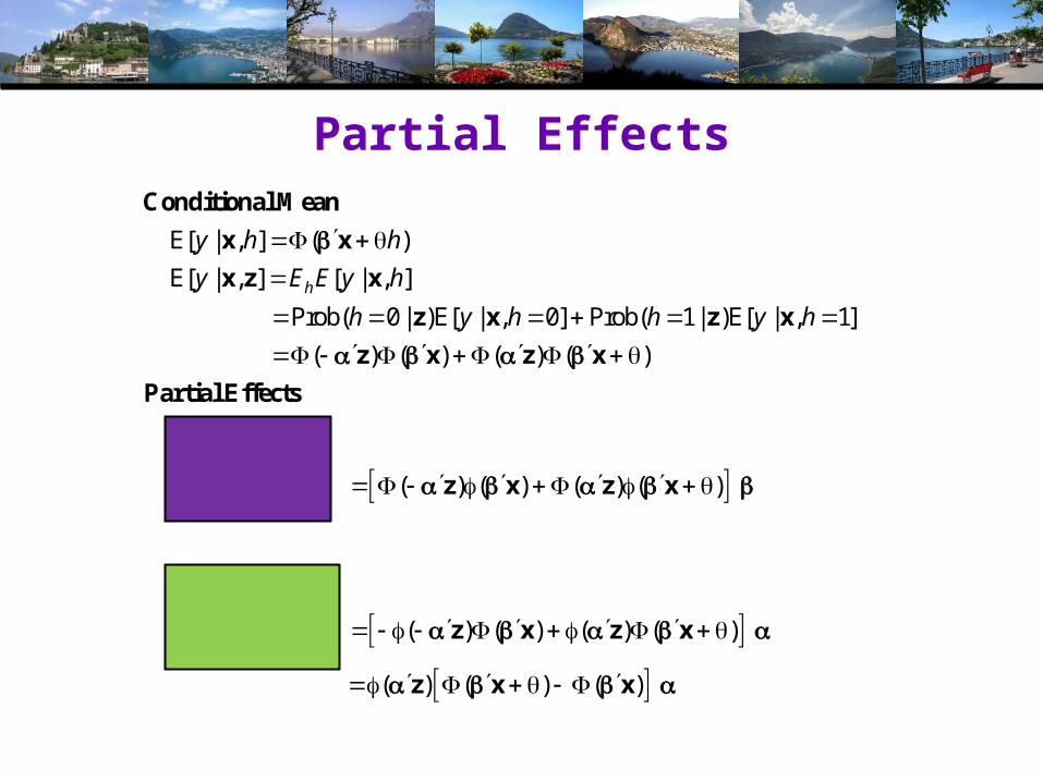
Partial Effects

E[ | , ] ( )

E[ | , ] [ | , ]

Prob( 0 | )E[ | , 0] Prob( 1| )E[ | , 1]

( ) ( ) ( ) ( )

h

y h h

y E E y h

h y h h y h

Conditional Mean

x x

x z x

z x z x

z x z x

Partial Effects

Direct Ef

E[ | , ] ( ) ( ) ( ) ( )

E[ | , ] ( ) ( ) ( ) ( )

( ) ( ) ( )

y

y

fects

x zz x z x

x

Indirect Effects

x zz x z x

zz x x

Identification Issues

• Exclusions are not needed for estimation• Identification is, in principle, by “functional form”• Researchers usually have a variable in the

treatment equation that is not in the main probit equation “to improve identification”

• A fully simultaneous model• y1 = f(x1,y2), y2 = f(x2,y1)• Not identified even with exclusion restrictions• (Model is “incoherent”)

Selection

A Sample Selection Model U* = β’x + ε

y = 1[U* > 0]h* = α’z + uh = 1[h* > 0]

E[ε|h] ≠ 0 Cov[u, ε] ≠ 0(y,x) are observed only when h = 1

Additional Assumptions: (u,ε) ~ N[(0,0),(σu

2, ρσu, 1)]

z = a valid set of exogenous variables, uncorrelated with (u,ε)

Correlation = ρ.This is the source of the “selectivity:

Application: Doctor,Public3 Groups of observations: (Public=0), (Doctor=0|Public=1), (Doctor=1|Public=1)

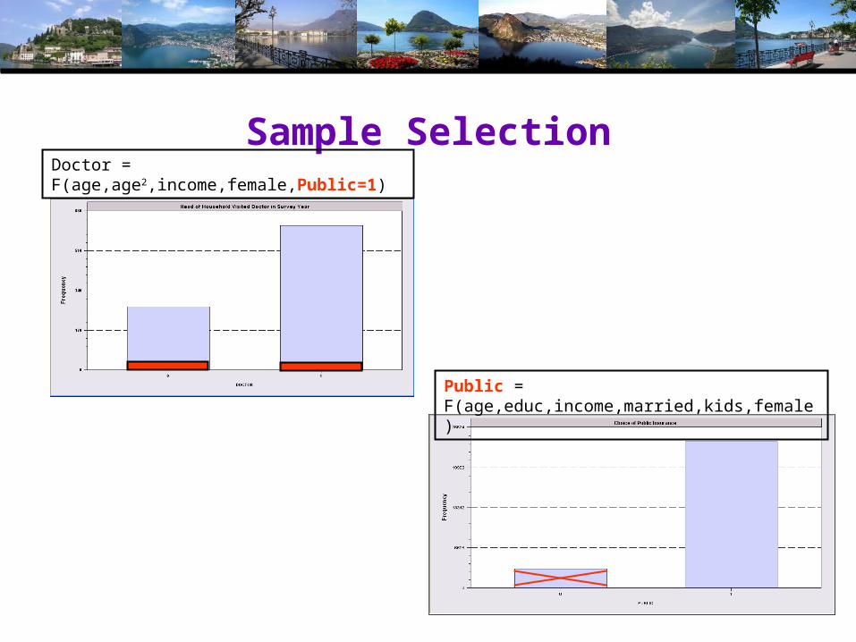
Sample SelectionDoctor = F(age,age2,income,female,Public=1)

Public = F(age,educ,income,married,kids,female)

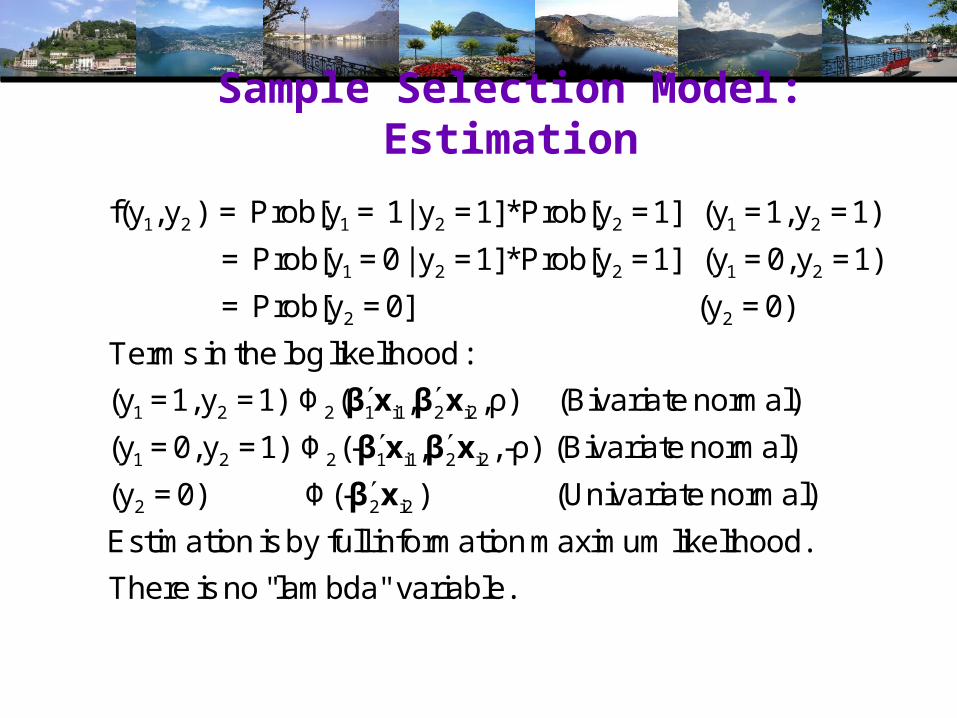
Sample Selection Model: Estimation

1 2 1 2 2 1 2

1 2 2 1 2

2 2

f(y ,y ) = Prob[y = 1| y =1] *Prob[y =1] (y =1,y =1)

= Prob[y = 0 | y =1] *Prob[y =1] (y = 0,y =1)

= Prob[y = 0] (y = 0)

Terms in the log likelih

1 2 2 1 i1 2 i2

1 2 2 1 i1 2 i2

2 2 i2

ood:

(y =1,y =1) Φ ( , ,ρ) (Bivariate normal)

(y = 0,y =1) Φ (- , ,-ρ) (Bivariate normal)

(y = 0) Φ(- ) (Univariate normal)

Estimation is by full inf

β x β x

β x β x

β x

ormation maximum likelihood.

There is no "lambda" variable.

ML Estimates----------------------------------------------------------------------FIML Estimates of Bivariate Probit ModelDependent variable DOCPUBLog likelihood function -23581.80697Estimation based on N = 27326, K = 13Selection model based on PUBLICMeans for vars. 1- 5 are after selection.--------+-------------------------------------------------------------Variable| Coefficient Standard Error b/St.Er. P[|Z|>z] Mean of X--------+------------------------------------------------------------- |Index equation for DOCTORConstant| 1.09027*** .13112 8.315 .0000 AGE| -.06030*** .00633 -9.532 .0000 43.6996 AGESQ| .00086*** .718153D-04 11.967 .0000 2041.87 INCOME| .07820 .05779 1.353 .1760 .33976 FEMALE| .34357*** .01756 19.561 .0000 .49329 |Index equation for PUBLICConstant| 3.54736*** .07456 47.580 .0000 AGE| .00080 .00116 .690 .4899 43.5257 EDUC| -.16832*** .00416 -40.490 .0000 11.3206 INCOME| -.98747*** .05162 -19.128 .0000 .35208 MARRIED| -.01508 .02934 -.514 .6072 .75862 HHKIDS| -.07777*** .02514 -3.093 .0020 .40273 FEMALE| .12154*** .02231 5.447 .0000 .47877 |Disturbance correlationRHO(1,2)| -.19303*** .06763 -2.854 .0043--------+-------------------------------------------------------------

Estimation Issues

• This is a sample selection model applied to a nonlinear model• There is no lambda• Estimated by FIML, not two step least squares• Estimator is a type of BIVARIATE PROBIT MODEL

• The model is identified without exclusions (again)

A Dynamic Model

Dynamic Models

it it i,t 1 it i

it i,t 1 i0 it it i,t 1 i

y 1[ y u > 0]

Two similar 'effects'

Unobserved heterogeneity

State dependence = state 'persistence'

Pr(y 1| y ,...,y ,x ,u] F[ y u]

How to estimate , , ma

x

x

rginal effects, F(.), etc?

(1) Deal with the latent common effect

(2) Handle the lagged effects:

This encounters the .initial conditions problem

Dynamic Probit Model: A Standard Approach

T

i1 i2 iT i0 i i,t 1 i itt 1

i1 i2 iT i0

(1) Conditioned on all effects, joint probability

P(y ,y ,...,y | y , ,u) F( y u ,y )

(2) Unconditional density; integrate out the common effect

P(y ,y ,...,y | y , )

i it

i

x x β

x

i1 i2 iT i0 i i i0 i

2i i0 i0 u i i1 i2 iT

i i0 i

P(y ,y ,...,y | y , ,u)h(u | y , )du

(3) Density for heterogeneity

h(u | y , ) N[ y , ], = [ , ,..., ], so

u = y + w (conta

i i

i i

i

x x

x x δ x x x x

x δ

it

i1 i2 iT i0

T

i,t 1 i0 u i it i it 1

ins every period of )

(4) Reduced form

P(y ,y ,...,y | y , )

F( y y w ,y )h(w )dw

This is a random effects model

i

it i

x

x

x β x δ

Simplified Dynamic Model

i

2i i0 i0 u

i i0 i

Projecting u on all observations expands the model enormously.

(3) Projection of heterogeneity only on group means

h(u | y , ) N[ y , ] so

u = y + w

(4) Re

i i

i

x x δ

x δ

i1 i2 iT i0

T

i,t 1 i0 u i it i it 1

duced form

P(y ,y ,...,y | y , )

F( y y w ,y )h(w )dw

Mundlak style correction with the initial value in the equation.

This is (again) a random effects mo

i

it i

x

x β x δ

del

A Dynamic Model for Public Insurance

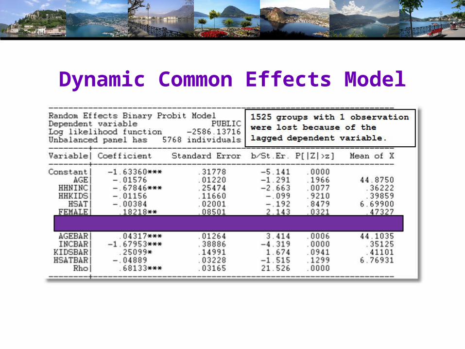
Dynamic Common Effects Model

BivariateModel

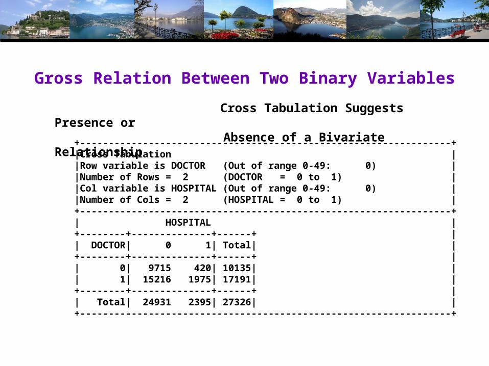
Gross Relation Between Two Binary Variables

Cross Tabulation Suggests Presence or Absence of a Bivariate Relationship

+-----------------------------------------------------------------+|Cross Tabulation ||Row variable is DOCTOR (Out of range 0-49: 0) ||Number of Rows = 2 (DOCTOR = 0 to 1) ||Col variable is HOSPITAL (Out of range 0-49: 0) ||Number of Cols = 2 (HOSPITAL = 0 to 1) |+-----------------------------------------------------------------+| HOSPITAL |+--------+--------------+------+ || DOCTOR| 0 1| Total| |+--------+--------------+------+ || 0| 9715 420| 10135| || 1| 15216 1975| 17191| |+--------+--------------+------+ || Total| 24931 2395| 27326| |+-----------------------------------------------------------------+

Tetrachoric Correlation

1 1 1 1 1

2 2 2 2 2

1

2

1

A correlation measure for two binary variables

Can be defined implicitly

y * =μ +ε , y =1(y * > 0)

y * = μ +ε ,y =1(y * > 0)

ε 0 1 ρ~ N ,

ε 0 ρ 1

ρ is the between y andtetrachoric correlation 2 y

Log Likelihood Functionfor Tetrachoric Correlation

n

2 i1 1 i2 2 i1 i2i=1

n

2 i1 1 i2 2 i1 i2i=1

i1 i1 i1 i1

2

logL = logΦ (2y -1)μ ,(2y -1)μ ,(2y -1)(2y -1)ρ

= logΦ q μ ,q μ ,q q ρ

Note : q = (2y -1) = -1 if y = 0 and +1 if y = 1.

Φ =Bivariate normal CDF - must be computed

using qu

1 2

adrature

Maximized with respect to μ ,μ and ρ.

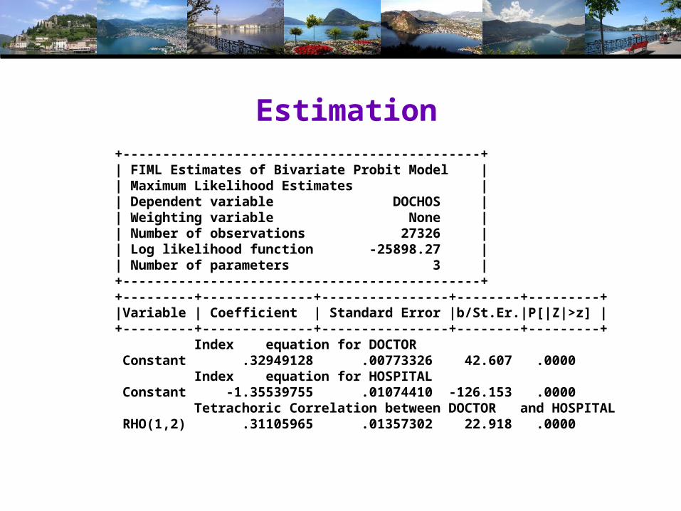
Estimation+---------------------------------------------+| FIML Estimates of Bivariate Probit Model || Maximum Likelihood Estimates || Dependent variable DOCHOS || Weighting variable None || Number of observations 27326 || Log likelihood function -25898.27 || Number of parameters 3 |+---------------------------------------------++---------+--------------+----------------+--------+---------+|Variable | Coefficient | Standard Error |b/St.Er.|P[|Z|>z] |+---------+--------------+----------------+--------+---------+ Index equation for DOCTOR Constant .32949128 .00773326 42.607 .0000 Index equation for HOSPITAL Constant -1.35539755 .01074410 -126.153 .0000 Tetrachoric Correlation between DOCTOR and HOSPITAL RHO(1,2) .31105965 .01357302 22.918 .0000

A Bivariate Probit Model

• Two Equation Probit Model• No bivariate logit – there is no

reasonable bivariate counterpart• Why fit the two equation model?

• Analogy to SUR model: Efficient• Make tetrachoric correlation conditional on

covariates – i.e., residual correlation

Bivariate Probit Model

1 1 1 1 1 1

2 2 2 2 2 2

1

2

2 2

y * = +ε , y =1(y * > 0)

y * = +ε ,y =1(y * > 0)

ε 0 1 ρ~ N ,

ε 0 ρ 1

The variables in and may be the same or

different. There is no need for each equation to have

its 'own vari

β x

β x

x x

.1 2

able.'

ρ is the conditional tetrachoric correlation between y and y

(The equations can be fit one at a time. Use FIML for

(1) efficiency and (2) to get the estimate of ρ.)

Estimation of the Bivariate Probit Model

i1 1 i1n

2 i2 2 i2i=1

i1 i2

n

2 i1 1 i1 i2 2 i2 i1 i2i=1

i1 i1 i1 i1

2

(2y -1) ,

logL = logΦ (2y -1) ,

(2y -1)(2y -1)ρ

= logΦ q ,q ,q q ρ

Note : q = (2y -1) = -1 if y = 0 and +1 if y = 1.

Φ =Bivariate normal CDF - must b

β x

β x

β x β x

1 2

e computed

using quadrature

Maximized with respect to , and ρ.β β

Parameter Estimates----------------------------------------------------------------------FIML Estimates of Bivariate Probit Model for DOCTOR and HOSPITALDependent variable DOCHOSLog likelihood function -25323.63074Estimation based on N = 27326, K = 12--------+-------------------------------------------------------------Variable| Coefficient Standard Error b/St.Er. P[|Z|>z] Mean of X--------+------------------------------------------------------------- |Index equation for DOCTORConstant| -.20664*** .05832 -3.543 .0004 AGE| .01402*** .00074 18.948 .0000 43.5257 FEMALE| .32453*** .01733 18.722 .0000 .47877 EDUC| -.01438*** .00342 -4.209 .0000 11.3206 MARRIED| .00224 .01856 .121 .9040 .75862 WORKING| -.08356*** .01891 -4.419 .0000 .67705 |Index equation for HOSPITALConstant| -1.62738*** .05430 -29.972 .0000 AGE| .00509*** .00100 5.075 .0000 43.5257 FEMALE| .12143*** .02153 5.641 .0000 .47877 HHNINC| -.03147 .05452 -.577 .5638 .35208 HHKIDS| -.00505 .02387 -.212 .8323 .40273 |Disturbance correlation (Conditional tetrachoric correlation)RHO(1,2)| .29611*** .01393 21.253 .0000---------------------------------------------------------------------- | Tetrachoric Correlation between DOCTOR and HOSPITALRHO(1,2)| .31106 .01357 22.918 .0000--------+-------------------------------------------------------------

Marginal Effects

• What are the marginal effects• Effect of what on what?• Two equation model, what is the conditional mean?

• Possible margins?• Derivatives of joint probability = Φ2(β1’xi1, β2’xi2,ρ) • Partials of E[yij|xij] =Φ(βj’xij) (Univariate probability)• Partials of E[yi1|xi1,xi2,yi2=1] = P(yi1,yi2=1)/Prob[yi2=1]

• Note marginal effects involve both sets of regressors. If there are common variables, there are two effects in the derivative that are added.

Bivariate Probit Conditional Means

i1 i2 2 1 i1 2 i2

i1 i2i1 1 i2 2

i

2 i2 1 i1i1 1 i1 2

Prob[y =1,y =1] = Φ ( , ,ρ)

This is not a conditional mean. For a generic that might appear in either index function,

Prob[y =1,y =1]= g +g

-ρg = φ( )Φ

1-ρ

β x β x

x

β βx

β x β xβ x

1 i1 2 i2i2 2 i2 2

1 i i1 2

2 1 i1 2 i2i1 i1 i2 i2 i1 i1 i2 i2

2 i2

i1 i1 i

-ρ,g = φ( )Φ

1-ρ

The term in is 0 if does not appear in and likewise for .

Φ ( , ,ρ)E[y | , ,y =1] =Prob[y =1| , ,y =1] =

Φ( )

E[y | ,

β x β xβ x

β x x β

β x β xx x x x

β x

x x 1

2 i2 2 1 i1 2 i2 2 i2i1 1 i2 2 22

i 2 i2 2 i2

i1 i2 2 1 i1 2 i2 2 i21 22

2 i2 2 i2 2 i2

,y =1] Φ ( , ,ρ)φ( )= g +g -

Φ( ) [Φ( )]

g g Φ ( x , x ,ρ)φ( x ) = + -

Φ( ) Φ( ) [Φ( )]

β x β x β xβ β β

x β x β x

β β ββ β

β x β x β x

Direct EffectsDerivatives of E[y1|x1,x2,y2=1] wrt

x1

+-------------------------------------------+| Partial derivatives of E[y1|y2=1] with || respect to the vector of characteristics. || They are computed at the means of the Xs. || Effect shown is total of 4 parts above. || Estimate of E[y1|y2=1] = .819898 || Observations used for means are All Obs. || These are the direct marginal effects. |+-------------------------------------------++---------+--------------+----------------+--------+---------+----------+|Variable | Coefficient | Standard Error |b/St.Er.|P[|Z|>z] | Mean of X|+---------+--------------+----------------+--------+---------+----------+ AGE .00382760 .00022088 17.329 .0000 43.5256898 FEMALE .08857260 .00519658 17.044 .0000 .47877479 EDUC -.00392413 .00093911 -4.179 .0000 11.3206310 MARRIED .00061108 .00506488 .121 .9040 .75861817 WORKING -.02280671 .00518908 -4.395 .0000 .67704750 HHNINC .000000 ......(Fixed Parameter)....... .35208362 HHKIDS .000000 ......(Fixed Parameter)....... .40273000

Indirect EffectsDerivatives of E[y1|x1,x2,y2=1] wrt

x2+-------------------------------------------+| Partial derivatives of E[y1|y2=1] with || respect to the vector of characteristics. || They are computed at the means of the Xs. || Effect shown is total of 4 parts above. || Estimate of E[y1|y2=1] = .819898 || Observations used for means are All Obs. || These are the indirect marginal effects. |+-------------------------------------------++---------+--------------+----------------+--------+---------+----------+|Variable | Coefficient | Standard Error |b/St.Er.|P[|Z|>z] | Mean of X|+---------+--------------+----------------+--------+---------+----------+ AGE -.00035034 .697563D-04 -5.022 .0000 43.5256898 FEMALE -.00835397 .00150062 -5.567 .0000 .47877479 EDUC .000000 ......(Fixed Parameter)....... 11.3206310 MARRIED .000000 ......(Fixed Parameter)....... .75861817 WORKING .000000 ......(Fixed Parameter)....... .67704750 HHNINC .00216510 .00374879 .578 .5636 .35208362 HHKIDS .00034768 .00164160 .212 .8323 .40273000

Marginal Effects: Total EffectsSum of Two Derivative Vectors

+-------------------------------------------+| Partial derivatives of E[y1|y2=1] with || respect to the vector of characteristics. || They are computed at the means of the Xs. || Effect shown is total of 4 parts above. || Estimate of E[y1|y2=1] = .819898 || Observations used for means are All Obs. || Total effects reported = direct+indirect. |+-------------------------------------------++---------+--------------+----------------+--------+---------+----------+|Variable | Coefficient | Standard Error |b/St.Er.|P[|Z|>z] | Mean of X|+---------+--------------+----------------+--------+---------+----------+ AGE .00347726 .00022941 15.157 .0000 43.5256898 FEMALE .08021863 .00535648 14.976 .0000 .47877479 EDUC -.00392413 .00093911 -4.179 .0000 11.3206310 MARRIED .00061108 .00506488 .121 .9040 .75861817 WORKING -.02280671 .00518908 -4.395 .0000 .67704750 HHNINC .00216510 .00374879 .578 .5636 .35208362 HHKIDS .00034768 .00164160 .212 .8323 .40273000

Marginal Effects: Dummy VariablesUsing Differences of Probabilities

+-----------------------------------------------------------+| Analysis of dummy variables in the model. The effects are || computed using E[y1|y2=1,d=1] - E[y1|y2=1,d=0] where d is || the variable. Variances use the delta method. The effect || accounts for all appearances of the variable in the model.|+-----------------------------------------------------------+|Variable Effect Standard error t ratio (deriv) |+-----------------------------------------------------------+ FEMALE .079694 .005290 15.065 (.080219) MARRIED .000611 .005070 .121 (.000511) WORKING -.022485 .005044 -4.457 (-.022807) HHKIDS .000348 .001641 .212 (.000348)

Computed using difference of probabilities

Computed using scaled coefficients

Simultaneous

Equations

A Simultaneous Equations Model

1 1 1 1 2 1 1 1

2 2 2 2 1 2 2 2

1

2

Simultaneous Equations Model

y * = + γ y +ε , y =1(y * > 0)

y * = + γ y +ε ,y =1(y * > 0)

ε 0 1 ρ~ N ,

ε 0 ρ 1

This model is not identified. (Not estimable.

The computer can compute 'e

β x

β x

stimates' but

they have no meaning.)

bivariate probit;lhs=doctor,hospital ;rh1=one,age,educ,married,female,hospital ;rh2=one,age,educ,married,female,doctor$Error 809: Fully simultaneous BVP model is not identified

Fully Simultaneous ‘Model’(Obtained by bypassing internal control)

----------------------------------------------------------------------FIML Estimates of Bivariate Probit ModelDependent variable DOCHOSLog likelihood function -20318.69455--------+-------------------------------------------------------------Variable| Coefficient Standard Error b/St.Er. P[|Z|>z] Mean of X--------+------------------------------------------------------------- |Index equation for DOCTORConstant| -.46741*** .06726 -6.949 .0000 AGE| .01124*** .00084 13.353 .0000 43.5257 FEMALE| .27070*** .01961 13.807 .0000 .47877 EDUC| -.00025 .00376 -.067 .9463 11.3206 MARRIED| -.00212 .02114 -.100 .9201 .75862 WORKING| -.00362 .02212 -.164 .8701 .67705HOSPITAL| 2.04295*** .30031 6.803 .0000 .08765 |Index equation for HOSPITALConstant| -1.58437*** .08367 -18.936 .0000 AGE| -.01115*** .00165 -6.755 .0000 43.5257 FEMALE| -.26881*** .03966 -6.778 .0000 .47877 HHNINC| .00421 .08006 .053 .9581 .35208 HHKIDS| -.00050 .03559 -.014 .9888 .40273 DOCTOR| 2.04479*** .09133 22.389 .0000 .62911 |Disturbance correlationRHO(1,2)| -.99996*** .00048 ******** .0000--------+-------------------------------------------------------------

A Latent Simultaneous Equations Model

*

*

1 1 1 1 2 1 1 1

2 2 2 2 1 2 2 2

1

2

Simultaneous Equations Model in the latent variables

y * = + γ y + ε , y =1(y * > 0)

y * = + γ y + ε , y =1(y * > 0)

ε 0 1 ρ~ N ,

ε 0 ρ 1

Note the underlying (latent) structural v

β x

β x

ariables in

each equation, not the observed binary variables.

This model is identified. It is hard to interpret. It can

be consistently estimated by two step methods.

(Analyzed in Amemiya (1979) and Maddala (1983).)

A Recursive Simultaneous Equations Model

1 1 1 1 1 1

2 2 2 2 1 2 2 2

1

2

Recursive Simultaneous Equations Model

y * = + ε , y =1(y * > 0)

y * = + γ y +ε ,y =1(y * > 0)

ε 0 1 ρ~ N ,

ε 0 ρ 1

It can be consisteThis model is identified.

β x

β x

ntly and efficiently

estimated by full information maximum likelihood. Treated as

a bivariate probit model, ignoring the simultaneity.

Ordered Choices

Ordered Discrete Outcomes

• E.g.: Taste test, credit rating, course grade, preference scale

• Underlying random preferences: • Existence of an underlying continuous preference scale• Mapping to observed choices

• Strength of preferences is reflected in the discrete outcome

• Censoring and discrete measurement• The nature of ordered data

Bond Ratings

Health Satisfaction (HSAT)Self administered survey: Health Satisfaction (0 – 10)

Continuous Preference Scale

Modeling Ordered Choices

• Random Utility (allowing a panel data setting)

Uit = + ’xit + it

= ait + it

• Observe outcome j if utility is in region j• Probability of outcome = probability of cell

Pr[Yit=j] = Prob[Yit < j] - Prob[Yit < j-1]

= F(j – ait) - F(j-1 – ait)

Ordered Probability Model

βx x

1

1 2

2 3

J-1 J

j-1

y* , we assume contains a constant term

y 0 if y* 0

y = 1 if 0 < y*

y = 2 if < y*

y = 3 if < y*

...

y = J if < y*

In general: y = j if < y*

j

-1 o J j-1 j

, j = 0,1,...,J

, 0, , , j = 1,...,J -1

Combined Outcomes for Health Satisfaction

Probabilities for Ordered Choices

j-1 j

j-1 j

j j 1

j j 1

j j 1

Prob[y=j]=Prob[ y* ]

= Prob[ ]

= Prob[ ] Prob[ ]

= Prob[ ] Prob[ ]

= F[ ] F[ ]

where F[ ] i

βx

βx βx

βx βx

βx βx

s the CDF of .

Probabilities for Ordered Choices

μ1 =1.1479 μ2 =2.5478 μ3 =3.0564

Coefficients

j 1 j kk

What are the coefficients in the ordered probit model?

There is no conditional mean function.

Prob[y=j| ] [f( ) f( )]

x

Magnitude depends on the scale factor and the coeff

xβ'x β'x

icient.

Sign depends on the densities at the two points!

What does it mean that a coefficient is "significant?"

Effects of 8 More Years of Education

An Ordered Probability Model for Health Satisfaction

+---------------------------------------------+| Ordered Probability Model || Dependent variable HSAT || Number of observations 27326 || Underlying probabilities based on Normal || Cell frequencies for outcomes || Y Count Freq Y Count Freq Y Count Freq || 0 447 .016 1 255 .009 2 642 .023 || 3 1173 .042 4 1390 .050 5 4233 .154 || 6 2530 .092 7 4231 .154 8 6172 .225 || 9 3061 .112 10 3192 .116 |+---------------------------------------------++---------+--------------+----------------+--------+---------+----------+|Variable | Coefficient | Standard Error |b/St.Er.|P[|Z|>z] | Mean of X|+---------+--------------+----------------+--------+---------+----------+ Index function for probability Constant 2.61335825 .04658496 56.099 .0000 FEMALE -.05840486 .01259442 -4.637 .0000 .47877479 EDUC .03390552 .00284332 11.925 .0000 11.3206310 AGE -.01997327 .00059487 -33.576 .0000 43.5256898 HHNINC .25914964 .03631951 7.135 .0000 .35208362 HHKIDS .06314906 .01350176 4.677 .0000 .40273000 Threshold parameters for index Mu(1) .19352076 .01002714 19.300 .0000 Mu(2) .49955053 .01087525 45.935 .0000 Mu(3) .83593441 .00990420 84.402 .0000 Mu(4) 1.10524187 .00908506 121.655 .0000 Mu(5) 1.66256620 .00801113 207.532 .0000 Mu(6) 1.92729096 .00774122 248.965 .0000 Mu(7) 2.33879408 .00777041 300.987 .0000 Mu(8) 2.99432165 .00851090 351.822 .0000 Mu(9) 3.45366015 .01017554 339.408 .0000

Ordered Probit Partial EffectsPartial effects at means of the data

Average Partial Effect of HHNINC

Predictions of the Model:Kids+----------------------------------------------+|Variable Mean Std.Dev. Minimum Maximum |+----------------------------------------------+|Stratum is KIDS = 0.000. Nobs.= 2782.000 |+--------+-------------------------------------+|P0 | .059586 .028182 .009561 .125545 ||P1 | .268398 .063415 .106526 .374712 ||P2 | .489603 .024370 .419003 .515906 ||P3 | .101163 .030157 .052589 .181065 ||P4 | .081250 .041250 .028152 .237842 |+----------------------------------------------+|Stratum is KIDS = 1.000. Nobs.= 1701.000 |+--------+-------------------------------------+|P0 | .036392 .013926 .010954 .105794 ||P1 | .217619 .039662 .115439 .354036 ||P2 | .509830 .009048 .443130 .515906 ||P3 | .125049 .019454 .061673 .176725 ||P4 | .111111 .030413 .035368 .222307 |+----------------------------------------------+|All 4483 observations in current sample |+--------+-------------------------------------+|P0 | .050786 .026325 .009561 .125545 ||P1 | .249130 .060821 .106526 .374712 ||P2 | .497278 .022269 .419003 .515906 ||P3 | .110226 .029021 .052589 .181065 ||P4 | .092580 .040207 .028152 .237842 |+----------------------------------------------+

This is a restricted model with outcomes collapsed into 5 cells.

Fit Measures

• There is no single “dependent variable” to explain.• There is no sum of squares or other measure of

“variation” to explain.• Predictions of the model relate to a set of J+1

probabilities, not a single variable.• How to explain fit?

• Based on the underlying regression• Based on the likelihood function• Based on prediction of the outcome variable

Log Likelihood Based Fit Measures

Fit Measure Based on Counting Predictions

This model always predicts the same cell.

A Somewhat Better Fit

Different Normalizations

• NLOGIT• Y = 0,1,…,J, U* = α + β’x + ε• One overall constant term, α• J-1 “thresholds;” μ-1 = -∞, μ0 = 0, μ1,… μJ-1, μJ = + ∞

• Stata• Y = 1,…,J+1, U* = β’x + ε• No overall constant, α=0• J “cutpoints;” μ0 = -∞, μ1,… μJ, μJ+1 = + ∞

α̂

ˆjμ

ˆ α

ˆˆjμ - α

Generalizing the Ordered Probit with Heterogeneous Thresholds

i

-1 0 j j-1 J

ij j

Index =

Threshold parameters

Standard model : μ = - , μ = 0, μ >μ > 0, μ = +

Preference scale and thresholds are homogeneous

A generalized model (Pudney and Shields, JAE, 2000)

μ = α +

β x

1 2 1 2

2 1 1

)

j

j

j i

ik i

ij i j ik ik

Note the identification problem. If z is also in (same variable) then

μ - = α + γz -βz +... E.g.,

( + Age + Married) - ( + Age Sex

( + Married) - ( + (

γ z

x

β x

2) )Age Sex

No longer clear if the variable is in or (or both)x z

Differential Item Functioning

People in this country are optimistic – they report this value as ‘very good.’

People in this country are pessimistic – they report this same value as ‘fair’

Panel Data

• Fixed Effects• The usual incidental parameters problem• Partitioning Prob(yit > j|xit) produces estimable

binomial logit models. (Find a way to combine multiple estimates of the same β.

• Random Effects• Standard application

Incidental Parameters Problem

Table 9.1 Monte Carlo Analysis of the Bias of the MLE in Fixed Effects Discrete Choice Models (Means of empirical sampling distributions, N = 1,000 individuals, R = 200 replications)

Random Effects

Dynamic Ordered Probit Model

Model for Self Assessed Health

• British Household Panel Survey (BHPS) • Waves 1-8, 1991-1998• Self assessed health on 0,1,2,3,4 scale• Sociological and demographic covariates• Dynamics – inertia in reporting of top scale

• Dynamic ordered probit model• Balanced panel – analyze dynamics• Unbalanced panel – examine attrition

Dynamic Ordered Probit Model

*, 1

, 1

, 1

Latent Regression - Random Utility

h = + + +

= relevant covariates and control variables

= 0/1 indicators of reported health status in previous period

H ( ) =

it it i t i it

it

i t

i t j

x H

x

H

*1

1[Individual i reported h in previous period], j=0,...,4

Ordered Choice Observation Mechanism

h = j if < h , j = 0,1,2,3,4

Ordered Probit Model - ~ N[0,1]

Random Effects with

it

it j it j

it

j

20 1 ,1 2

Mundlak Correction and Initial Conditions

= + + u , u ~ N[0, ]i i i i i H x

It would not be appropriate to include hi,t-1 itself in the model as this is a label, not a measure

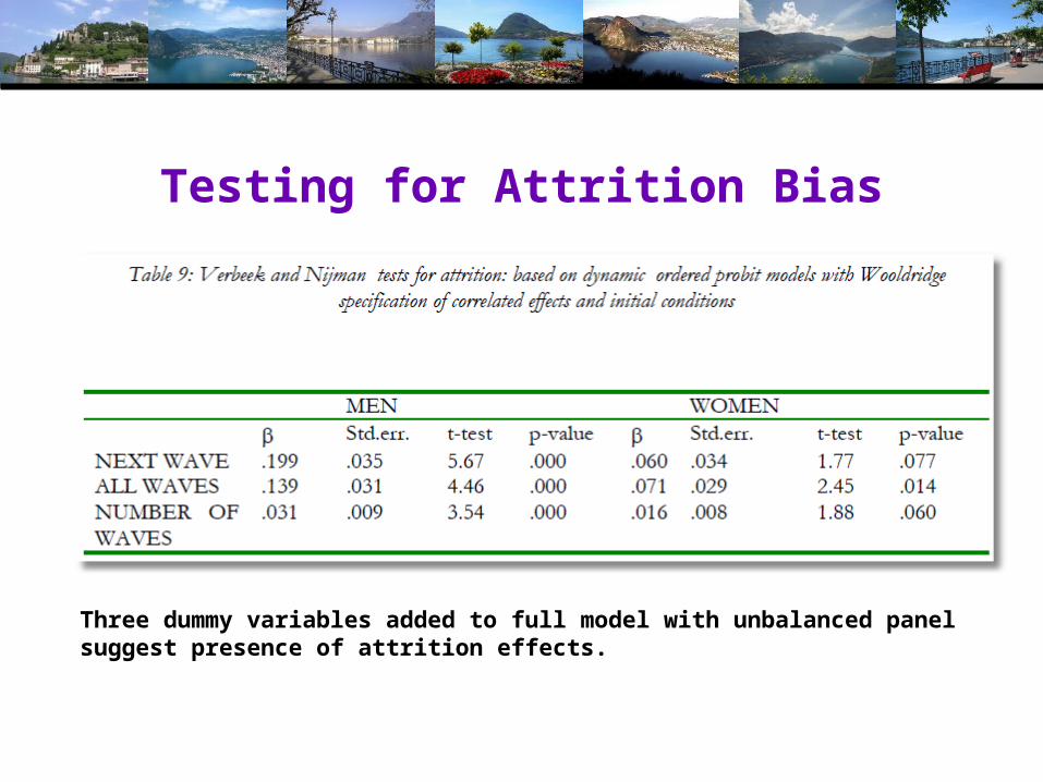
Testing for Attrition Bias

Three dummy variables added to full model with unbalanced panel suggest presence of attrition effects.

Attrition Model with IP Weights

Assumes (1) Prob(attrition|all data) = Prob(attrition|selected variables) (ignorability) (2) Attrition is an ‘absorbing state.’ No reentry. Obviously not true for the GSOEP data above.Can deal with point (2) by isolating a subsample of those present at wave 1 and the monotonically shrinking subsample as the waves progress.

Inverse Probability WeightingPanel is based on those present at WAVE 1, N1 individuals

Attrition is an absorbing state. No reentry, so N1 N2 ... N8.

Sample is restricted at each wave to individuals who were present at

the pre

1 , 1

1

vious wave.

d = 1[Individual is present at wave t].

d = 1 i, d 0 d 0.

covariates observed for all i at entry that relate to likelihood of

being present at subsequen

it

i it i t

i

x

t waves.

(health problems, disability, psychological well being, self employment,

unemployment, maternity leave, student, caring for family member, ...)

Probit model for d 1[it i x 1

1

ˆ], t = 2,...,8. fitted probability.

ˆ ˆAssuming attrition decisions are independent, P

dˆInverse probability weight WP̂

Weighted log likelihood logL log (No common

it it

t

it iss

itit

it

W it

w

L

8

1 1 effects.)

N

i t

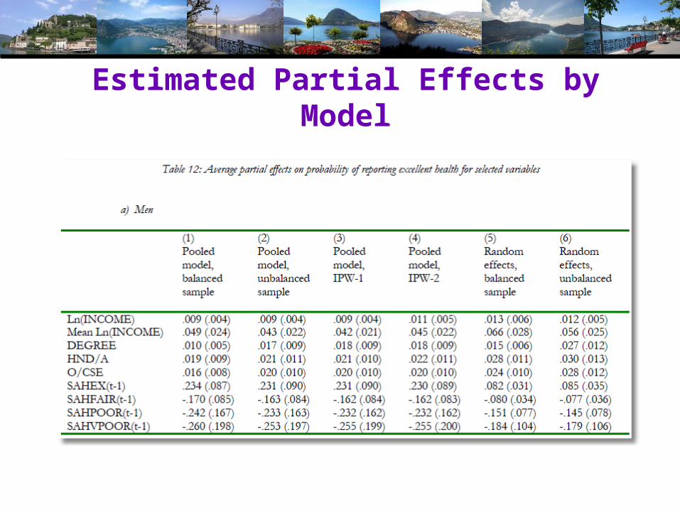
Estimated Partial Effects by Model

Partial Effect for a Category

These are 4 dummy variables for state in the previous period. Using first differences, the 0.234 estimated for SAHEX means transition from EXCELLENT in the previous period to GOOD in the previous period, where GOOD is the omitted category. Likewise for the other 3 previous state variables. The margin from ‘POOR’ to ‘GOOD’ was not interesting in the paper. The better margin would have been from EXCELLENT to POOR, which would have (EX,POOR) change from (1,0) to (0,1).