emerging markets and the global economy || measuring systemic risk in emerging markets using covar

CHAPTER1212Measuring Systemic Risk in EmergingMarkets Using CoVaRAnastassios A. Drakos* and Georgios P. Kouretas**Department of Business Administration, Athens University of Economics and Business, Athens, Greece

1. INTRODUCTION

The global financial crisis of 2007–2009 illustrated how distress can spread quickly throughthe financial system and threaten financial stability. Furthermore, Brunnermeier andPedersen (2009) argue that the degree to which international financial institutions arelinked depends on the level of market liquidity. Banks play a crucial role in the properfunctioning of an economy because they provide the necessary liquidity to the marketsand help to promote economic growth (Levine, 1997). Ill-functioning of the bankingsector dramatically increases the costs in the real economy and historically has been amajor source of financial crises, like the recent one, in both developed and emergingeconomies (Barth and Caprio, 2006; Demirguc-Kunt et al., 2009; Reinhart and Rogoff,2009). Since October 1987, financial and banking regulation has focused on monitoringand regulating the banking industry.

The recent financial crisis revealed that the micro-prudential regulatory framework isnot sufficient to prevent worldwide contagion as a result of bank failures initially in the USand subsequently in Europe and elsewhere. The micro-prudential regulatory frameworkis based on the provisions of the Basle I and II agreements which imposed minimumcapital requirements on the banks as a measure of prevention against unexpected losses(Pillar I). Within this framework, the Basle II agreement led to the development ofinternal systems for the measurement of market risk and such a regulation looked at thesoundness of individual financial institutions. However, such provisions based only oncapital adequacy ignored factors such as size, degree of leverage, and interrelationshipswith the rest of the system. Stein (2010, p. 50) argued that “the overarching goal offinancial reform must not be only to fortify a set of large institutions, but rather to reducethe fragility of our entire system of credit creation.”

Thus, there is now a shift in macro-prudential regulation, which implies that weobserve the operation of the banking system as a whole (see Borio and Lowe, 2002;Borio and Drehmann, 2009; Gauthier et al., 2012). The Bassle III agreement which isstill under formation is expected to address most of the issues related to systemic riskand develop the appropriate framework for regulation and supervision of the financial

Emerging Markets and the Global Economy © 2014 Elsevier Inc.http://dx.doi.org/10.1016/B978-0-12-411549-1.00012-0 All rights reserved. 271

http://dx.doi.org/10.1016/B978-0-12-411549-1.00012-0

272 Anastassios A. Drakos and Georgios P. Kouretas

markets based on recent experience.Therefore, for Central Banks and financial regulators,it is of great value to be able to quantify the risks that can threaten the financial system,not only at the national level but also globally. Early works on this front by Lehar (2005),Goodhart et al. (2005, 2006), and Goodhart (2006) proposed alternative measures offinancial fragility which can be implemented at both the individual and the aggregatelevels. Additionally, the Financial Sector Assessment Program (a joint IMF and WorldBank initiative) was set up with the purpose of increasing the effectiveness of plans topromote the soundness of financial systems in their member countries.

Interdependence among financial institutions becomes particularly important duringperiods of distress, when losses tend to spread across institutions and the whole financialsystem becomes vulnerable. In this respect, systemic risk is defined as multiple simultan-eous defaults of large financial institutions. A systemic crisis that disrupts the stability ofthe financial system can have serious consequences and large costs for the whole economyand the society. During financial crises, episodes of contagion among financial institu-tions occur very often and therefore regulators need to take them into considerationwhen assessing the health of the financial system. Central banks are responsible for pro-moting financial stability in the domestic economy and hence it is a central componentof the central banks’ activities to follow and analyze systemic risk. The financial crisis of2007–2009 has put increased emphasis on analyzing systemic risk and developing sys-temic risk indicators that can be used by central banks and others as a monitoring tool.In order to evaluate the stability of the banking system, a crucial element is the measure-ment of the systemic risk of a financial system. According to the Group of Ten (2001,p.126):

Systemic financial risk is the risk that an event will trigger a loss of economic value or confidencein, and attendant increases in uncertainly [sic] about, a substantial portion of the financial systemthat is serious enough to quite probably have significant adverse effects on the real economy.Systemic risk events can be sudden and unexpected, or the likelihood of their occurrence can buildup through time in the absence of appropriate policy responses. The adverse real economic effectsfrom systemic problems are generally seen as arising from disruptions to the payment system, tocredit flows, and from the destruction of asset values.

Arnold et al. (2012) also argue that key aspects of recent regulatory reforms which areunder way through the Basle III agreement include measuring and regulating systemicrisk and designing and implementing macro-prudential policies in an appropriate way.To this end the EU has established the European Systemic Risk Board and the US theFinancial Stability Oversight Council in order to focus on the issue of systemic risknot only in those two regions but also at the global level. The collapse of numerousfinancial institutions over the last 5 years has imposed significant negative spillovers ongovernments and the economy as a whole. Therefore, in measuring systemic risk weneed to consider the degree of risk of financial institutions and to allocate risks and costs

Measuring Systemic Risk in Emerging Markets Using CoVaR 273

across them so that we take into account the negative spillovers associated with financialinstability. Although the issue of stability of the banking sector is very important, thereare only a few studies that examine the impact of bank regulation and supervision onbanking risk, some of which find that it has little effect on minimizing banking risk.Thus,Demirguc-Kunt and Detragiache (2011),using a sample of 3000 banks from 86 countries,reject the hypothesis that better regulation and supervision results in a sounder bankingsystem. In contrast,Klomp and de Haan (2012) also examine the issue of the effectivenessof bank regulation and supervision and find evidence in favor of its effectiveness for high-risk banks. However, when they consider low-risk banks then they find no support infavor of the effectiveness of the regulatory framework.

The most commonly used measure of market risk is theValue-at-Risk (VaR) whichcalculates the monetary loss an institution may experience within a given confidencelevel. The problem with such a measure is that it does not consider the institution aspart of a system which might itself experience instability and spread new sources of eco-nomic risk. Furthermore, it is noted that traditional measures have focused on banks’ bal-ance sheet information, including non-performing loans ratios, earnings and profitability,liquidity and capital adequacy measures which are not appropriate to evaluate the sound-ness of a financial system (see Huang et al., 2009; Sylvain et al., 2012).

Recently, Adrian and Brunnermeier (2011) developed CoVaR as a measure of sys-temic risk. CoVaR measures the contribution of a financial institution to systemic riskand its contribution to the risk of other financial institutions. CoVaR stands for Con-ditional Value-at-Risk, and indicates the Value-at-Risk (VaR) of financial institution i,conditional on financial institution j being in distress. Adrian and Brunnermeier (2011)argue that this is a more complete measure of risk since it is able to capture alterna-tive sources of risk which affect institution i even though they are not generated by it.Furthermore, if we consider that institution i is the whole financial system,then �CoVaRis defined as the difference between the CoVaR and the unconditionalVaR and it capturesthe marginal non-causal contribution of a particular institution to the overall systemic risk.

In this chapter, we build on the CoVaR methodology which allows us to generatetime-varying estimates of the systemic risk contribution of three specific sectors of thefinancial industry subject to different regulation and supervisory framework:banks, insur-ances, and financial services. We employ weekly data from December 1995 to February2013 for selected countries from a group of emerging economies from Latin America,Central and Eastern Europe, and Southeast Asia which have been seriously affected bythe recent financial crisis. Furthermore, the purpose of the analysis is to examine whetherthe contribution of the different financial sectors has changed following the failure ofLehman Brothers in September 2008. Applying the CoVaR analysis we want to measurerisk spillovers and model the conditional second moments of the financial sectors on thewhole economy.


There are several important findings that stem from our analysis. First, the estimationsof 1% and 50% quantile regressions show that equity returns are a key determinant intriggering systemic risk episodes.There is also evidence that volatility of the general indexex financials (system variable), liquidity spread, the three-month rate change, and yieldspread have an effect, although weaker. Second, we show that for Mexico, the CzechRepublic, Hungary, Romania, Hong Kong, Indonesia, the Philippines, and Thailand it isthe banking sector that contributes mostly to the systemic risk. In Malaysia, the insuranceindustry contributes most to the systemic risk,whereas in Poland,Turkey,Korea,Malaysia,and Singapore the highest percentage contribution to systemic risk is due to the otherfinancial services. Finally,based on the results of �CoVaR estimates before and after 2008,it is observed that for all emerging markets the contribution of each financial industry tosystemic risk increased after the unfolding of the crisis.

The structure of the chapter is as follows: Section 2 presents and discusses the recentliterature on CoVaR modeling. Section 3 discusses the CoVaR modeling approach toestimate systemic risk. Section 4 presents the data and empirical results while a summaryand Section 5 gives the concluding remarks.

2. REVIEWOF THE LITERATURE

Achieving macroeconomic stability requires the identification of systemic risk in thefinancial system and the factors driving it.Although there is no consensus on the definitionand measurement of systemic risk, we review the recent literature on the topic in thissection (for a complete survey, see Bisias et al., 2012).

The recent literature has followed two main channels to analyze systemic risk. First,several studies examine the channels through which risk is transmitted from one finan-cial institution to another. Pritsker (2000) and Forbes and Rigobon (2001) were amongthe first studies to explain the transmission of disturbances from one market to anotherover time, identifying two transmission channels which take the form either of inter-dependence or contagion. Within this framework we also observed the development ofresearch on early warning indicators for both developed and emerging economies inan attempt to forecast systemic events (see, for example, Borio and Lowe, 2002; Alessiand Detken, 2009; Alfaro and Drehmann, 2009, Borio and Drehmann, 2009; Gieseckeand Kim, 2011; Huang et al., 2009; Khandani et al., 2010; Borio et al., forthcoming). Asecond approach of measuring systemic risk using either macroeconomic data or balancesheet data has also been employed but suffers from two shortcomings.Thus,Cerutti et al.(2011) emphasize the problem that researchers face with the lack of useful and consistentdata and suggest the creation of a common reporting template for globally systematicallyimportant financial institutions. A second shortcoming of this approach lies in the staticmodeling of institutional behavior and therefore models with low-frequency data are notappropriate for studying the effects of the regulatory and supervisory framework.


The second strand of literature on measuring systemic risk uses high-frequency timeseries data. Several approaches have been proposed. Segoviano and Goodhart (2009) andMoreno and Peña (2013) argue that CDS spreads are good estimators of systemic risk.The problem with this approach is that it captures only credit risk and not market risk,which is the issue under examination in the present paper. Another approach focuseson individual measures of systemic risk, which seek to predict how much the stocks offinancial institutions fall in a major market downturn. Essentially, this approach providesa framework to evaluate the co-dependence of financial institutions on a given systemwhen a distress event occurs.The theoretical foundations of this approach were developedin Acharya and Richardson (2009), Acharya et al. (2010), and Acharya et al. (2012).Acharya et al. (2010) define the systemic expected shortfall as the propensity of a financialinstitution to be undercapitalized when the system as a whole is undercapitalized. Inaddition, Acharya et al. (2012) show that when this negative event occurs,the governmentusually wants to minimize the resulting cost to the taxpayer. Furthermore, it is shownthat this cost is a function of size, leverage, and expected equity losses during a crisis.Brownlees and Engle (2012) propose a bivariate GARCH model for volatility as well asan asymmetric DCC model to capture correlation. Furthermore, they construct short-and long-run Marginal Expected Shortfall forecasts and propose the SRISK index,whichis also a distress measure.

Adrian and Brunnermeier (2011) propose the CoVaR methodology in order to eval-uate the impact of financial units which are in distress on the whole financial system.Therefore, this approach is useful in measuring risk transmission from a financial insti-tution to the financial system. For their empirical application they use quantile regres-sions to estimate the conditional models using data for 1266 US financial institutionswhich are distinguished into four groups: commercial banks, broker-dealers (includingthe investment banks), insurance companies, and real estate.They conclude that systemicrisk depends significantly on size, leverage, and maturity mismatch. This methodologyhas been applied in several recent studies.Van Oordt and Zhou (2010) extended CoVaRto analyze situations at an extremely low probability level. Their analysis is based on46 equally weighted industry portfolios including NYSE,AMEX, and NASDAQ firms.Wong and Fong (2010) examine the interrelationships among 11 Asia-Pacific economiesby estimating CoVaR for the CDS of their banks.Their main finding is that CoVaR mea-surements are higher than the respective unconditionalVaR measure. Chan-Lau (2008)using a similar approach, studied the existence of spillover effects using the CDS spreadsof a sample of 25 financial institutions in Europe, Japan, and the United States.

Recently,Agrippino (2009) proposed the implementation of CoVaR analysis of fiveUS commercial banks using daily data in order to distinguish between interdependenceand spillovers among financial institutions. The analysis concludes that CoVaR providessuperior measurement of risk compared with the estimated with the traditional VaRmodel, particularly in case of financial instability when negative effects are spread across


institutions. Roengpitya and Rungcharoenkitkul (2011) employ panel data from six majorbanks of Thailand in order to examine risk spillover effects among these financial institu-tions. Girardi and Ergun (2013) modified the CoVaR model.They change the definitionof financial distress from a financial institution i to a financial institution j as being higher,instead of being equal, than its VaR estimate. They estimate the systemic risk contri-butions of four financial industry groups consisting of a large number of institutions.Lopez-Espinoza et al. (2012a) analyze the banking system responses to positive and neg-ative shocks to the market-value balance sheets of individual banks. Lopez-Espinoza et al.(2012b) employ an asymmetric CoVaR methodology to deal with a representative sam-ple of 54 international banks and to address the asymmetric patterns that may underlietail dependence. Bjarnadottir (2012) studies the contribution of four major Swedish banksto the systemic risk of the Swedish financial system. Finally, Bernal et al. (2012) departfrom the above-mentioned papers since they study systemic risk by analyzing how finan-cial sectors of an economy that operate under different regulation systems contribute tosystemic risk. Therefore, they examine the existence of interrelationships between thefinancial sector and the whole, instead of focusing on individual institutions. They esti-mate the respective CoVaR model using daily data for the banking, insurance, and otherfinancial services industries of the US and the Eurozone, and they find that the insurancesector contributes relatively more to the systemic risk in periods of distress comparedwith the banking and other financial services industries.

This chapter adopts the approach suggested by Bernal et al. (2012) in evaluating thecontribution to systemic risk by different aggregated components of the financial systemincluding the banking, insurance, and other financial services industries. The argumentthat Bernal et al. (2012) make is that the evaluation of the impact of shocks affecting oneof these different financial industries on the whole system is important in designing anappropriate regulation. We employ CoVaR analysis to study the impact of these threefinancial sectors on the whole system for a selected group of emerging markets fromthree regions: Latin America, Central and Eastern Europe, and Southeast Europe.

To the best of our knowledge, this is the first study that provides an analysis of assessingsystemic risk for the case of emerging markets, since all aforementioned studies focusedexclusively on developed economies. This is due to the fact that the recent crisis is oneof the few if not the first one whose source is the developed economies and not theemerging economies. Therefore, the propagation mechanism is from the US and theEurozone to the emerging markets. The recent banking crisis in Cyprus (a membercountry of the Eurozone) came with a possible 5-year delay from the initial shock. Itwas partly caused by the Eurozone debt crisis and more specifically as an outcome of theGreek debt crisis since the “haircut” on the Greek long-term sovereign bonds that tookplace in March 2012 imposed a loss of 4.5 billion euros on the banking system of Cyprus.The emerging economies suffered substantial losses since the credit crunch of 2007–2008and the collapse of Lehman Brothers in September 2008.These negative effects have not


been symmetric to the different groups of emerging markets. In particular, the economiesof the Central and Eastern European countries had to undergo major adjustment in theirfinancial sectors and their real economies as a whole because of the recent financialand debt crisis. Countries like Hungary and Estonia almost went bankrupt and had todevalue their currency up to 30%.The Czech Republic, Poland, and Romania also facedsimilar adjustments. LatinAmerica countries were also hit by the credit crunch which wasevident,for example,inArgentina where the long adjustment process to return to financialmarkets following the 2001 collapse has deteriorated once again. The Southeast Asiancountries were also affected, although in a milder way, particularly with the experienceof increased volatility in their stock markets.

3. ECONOMETRICMETHODOLOGY

During the last 15 years there has been a voluminous literature on measuring approacheson market risk and propagation channels and causes of risk contagion effects. However, ithas been shown that these traditional approaches have several modeling limitations,as wellas strong assumptions with respect to the returns distribution and thus their applicationwas proven problematic. Following the Basle II agreement, the Value-at-Risk measurebecame very popular to measure market risk because of its simplicity since the calculationof a single number was considered to be sufficient to quantify the minimum capitaladequacy requirements for a financial institution. Intuitively, theVaR(α) is the worst lossover a target horizon that will not be exceeded with a given level of confidence 1 − α

( Jorion, 2007). Statistically, theVaR(α) defined for a confidence level 1 − α correspondsto the α-quantile of the projected distribution of gains and losses over the target horizon.

This was the main approach used within the context of micro-prudential regulationas proposed by the Basle I and Basle II agreements. First, VaR models only estimatetheir own minimum loss if tail takes place under several alternative error distributionspecifications. However, these models do not bring to the surface the potential loss ofsystemic risk transmitted from other sectors of either the domestic economy or the globaleconomy.A stylized fact of these models is that the error terms of the dynamic correlationmodel or the autoregressive conditional heteroskedasticity model are assumed to have aspecific distribution which leads to a bias toward the coefficients’ estimation. Second,the extreme value theory and the derived models for estimating VaR do not take intoconsideration the full set of observations of the sample, leading to an underestimation ofthe respective risk measure, whereas there is also a small sample bias (see, for example,Wong and Fong, 2010). A final critical issue on modeling interrelationships betweendifferent sectors of the economy refers to time lag.

Given these criticisms regarding the ability of the traditional VaR model to capture sys-temic risk,we employ the CoVaR model (Adrian and Brunnermeier, 2011).The CoVaRmodel is particularly useful for measuring systemic risk by the VaR of an institution


conditional on other institutions being in distress. During the 2007–2009 global finan-cial crisis, the emerging economies faced severe credit risk and major financial problems.Therefore, the CoVaR model is appropriate to study risk spillovers and therefore is alsoa convenient measure of systemic risk.

Following Adrian and Brunnermeier (2011) we define CoVaRj|iq , which implies that

theVaRjq of an institution j (or of the financial institution) conditional on institution i’s

event C(Ri) which is realized by the returns for this institution (Ri) being equal to itslevel of VaR for a qth quantile Ri = VaRi

q. CoVaRj|iq is then the qth quantile of the

conditional probability distribution of returns of j:

P(Rj ≤ CoVaRj|C(Ri)q |C(Ri)) = q. (1)

Adrian and Brunnermeier (2011) define �CoVaR as the difference between theCoVaR of the financial institution j conditional on the distress of another institutioni and CoVaR of institution j conditional on the normal state of institution i. Therefore,this CoVaR measurement calculates how much an institution contributes to anotherinstitution’s risk:

�CoVaRj|iq = CoVaR

j|Xi=VaRiiq

q − CoVaRj|Xi=Mediani

q , (2)

where �CoVaRj|iq denotes the VaR of institution j’s asset returns when institution i’s

returns are at its normal state of their distribution (e.g. 50% percentile), and �CoVaRj|iq

is institution j’s VaR when institution i’s returns are in a distressed or extremely badcondition like the one experienced during the recent financial crisis. It can also betaken as the additional VaR caused by outside influences, which is above the ordinaryinterdependencies.

We further calculate �CoVaR for each institution as follows:

�CoVarj|it (q) = CoVaRj|i

t (q) − CoVaRj|it (50%) = β̂ j|i[VaRi

t(q) −VaRit(50%)]. (3)

Adrian and Brunnermeier (2011) estimate the related VaRj|iq and their �CoVaRj|i

qwith the use of the growth rates of market-valued total assets for an individual institutionand define them as a function of a constant, lagged state variables, and error term. Inorder to assess the link between a set of independent variables and the quantiles of thedependent variable, they employ the quantile regressions methodology developed byKoenker and Basset (1978) and Koenker (2005).

In this chapter, we depart from Adrian and Brunnermeier (2011), who focus onthe financial system, and we consider the real economy as the system variable. Recently,Bernal et al. (2012) defined systemic risk as the impact that a group of financial institutionsmay have on the whole economy. In this context, systemic risk is measured with the


estimation of �CoVaR. Based on equations (1) and (2) we define CoVaRsystem|iq as the

VaRsystemq of the whole system conditional on an event C(Ri) affecting a financial sector i

being equal to its level of VaR for a qth quantile.This is given by the following probability:

P(Rsystem ≤ CoVaRsystemC(Ri)q |C(Ri) = q. (4)

Therefore,

�CoVaRsystem|iq = CoVaR

system|Xi=VaRiiq

q − CoVaRsystem|Xi=Mediani

q . (5)

Following Bernal et al. (2012) we use this modeling approach to assess risk transmissionfrom a given financial sector to the whole economy in selected emerging economiesof Latin America, Central and Eastern Europe, and South East Asia. The econometricapproach is implemented in five stages.

The first stage deals with modeling the returns Ri as a function of a set of state variables:

Rit = αi + γ iMt + εi

t, (6)

where αi is the constant, Mt represents a vector of contemporaneous control variables,and εi

t is a white noise error term. We then estimate the 1% quantile of market returnbased on the quantile regressions.

The second step involves the computation of the predicted 1% VaR for each segmentof the financial system using only the statistically significant variables that were identifiedin the first stage. Given that the VaR(α) defined for a confidence level 1 − α is thequantile of the distribution of gains and losses over the target horizon, the forecast willbe obtained as follows:

ˆVaR = α̂i + γ̂ iMt, (7)

where α̂i and γ̂ i are the coefficient estimates from equation (6).We then move to third stage of our analysis in which we estimate the system’s returns

using the following equation:

Rsystemt = αsystem|i + β system|iRi

t + γ system|iMt + εsystem|it , (8)

where αsystem|i is the constant, β gives the contribution of the return Rit of each financial

sector to the real economy, Mt is a set of contemporaneous control variables, and εsystem|it

is a white noise error term.Again the 1% quantile of returns is obtained from the quantileregression.

In the next stage, we compute the CoVaR of the system which is the VaR of thesystem conditional with a situation of distress within either one of the individual financialsectors, represented by the 1% quantiles computed in the previous stages. Therefore, theestimation of CoVaR requires the use of the computed VaR (1%) from equation (7),given all the significant control variables obtained from equation (8):


ˆCoVaRit = α̂sytem|i + β̂ systemi ˆVaR

it + γ̂ system|iMt, (9)

where α̂system|i, β̂ system|i and γ̂ system|i are derived from equation (8).The fifth and final stage of the estimation process involves the computation of �CoVaR

which, as we explained above, is the difference between the CoVaR at the 1% quantileand the CoVaR at the 50% quantile. The calculation of CoVaR at the 50% quantile ismade using the same approach, with the only difference being that we take 50% of thereturns at each step. This CoVaR at the 50% quantile describes a conditional event at amedian state given in formulation (5) which is required in order to compute the systemicrisk measure. �CoVaR is the marginal contribution of each financial sector to systemicrisk, i.e.:

ˆ�CoVaRit(q) = ˆCoVaR

it(1%) − ˆCoVaR

it(50%). (10)

During a financial crisis,portfolio returns of all financial institutions are at theirVaR level.Therefore, the CoVaR model is particularly appropriate for capturing risk contagion froma systemic crisis. Because the credit risk faced by financial institutions is more severe whenthere is a dramatic fall in prices and therefore returns, we focus on the downside risk ofthe changes in prices and thus, ˆ�CoVaR takes negative values because it is computedfrom the 1% returns of each financial industry. Within this framework, we consider thatthe financial sector with the larger absolute ˆ�CoVaR is the sector that contributes themost to systemic risk in periods of distress.

4. DATA AND EMPIRICAL RESULTS

We analyze the effect that three segments of the financial industry, namely banking,insurance, and financial services sectors, have on the whole economy. It is interesting tonote that these three sectors are subject to different regulatory frameworks. We employour analysis for three groups of emerging markets: in Latin America, South East Asia, andCentral and Eastern Europe. We use weekly data from December 29, 1995 to March 1,2013.We will thus be able to provide evidence as to whether there is a shift in the evidencebefore and after 2008, which will indicate whether or not systemic risk increased afterthe financial crisis.1

The first set of variables (Rit s) consists of the returns of the three financial sectors and

of the system. Specifically, for each country we employ the Banks index, the Insurances

1 Due to data availability the countries used in the present analysis are: Mexico, the Czech Republic, Hungary, PolandRomania,Turkey, Hong Kong, Indonesia, Korea, Malaysia, the Philippines, Singapore, and Thailand. The same holdsfor the sample used in the estimations. The number of observations used also depends on data availability. We usehigh-frequency weekly data in order to obtain a reactive measure of systemic risk. Alternatively, we could use dailydata but the problem is that the bond markets in these emerging economies are not very liquid and we would unableto capture substantial reaction and volatility of the stock market indices.


index and the Financial Services index, whereas the system variable is proxied by thegeneral stock returns index excluding the Financials index.2

In order to estimate the time-varying CoVaRt andVaRt , we include a set of controlvariables Mt .These variables are taken to capture time variation in conditional momentsof asset returns and at the same time are liquid and tradable.These control variables Mt aregiven as follows: (1) Liquidity spread, which measures short-term liquidity risk, is definedas the difference between the three-month repo rate and the three-month treasury billrate. (2) three-month treasury bill spread variation is defined as the difference between thethree-month bond rate in time t and the three-month bond rate in time t −1. FollowingAdrian and Brunnermeier (2011) we use the change in the three-month treasury bill,because the change and not the level is considered to be more significant in explainingthe tails of financial sector market-valued asset returns. (3)Yield spread change is definedas the difference between the 10-year or 5-year government bond rate (depending onthe availability of data) and the three-month treasury bill rate. This measure captures thechange in the slope of the yield curve. (4) Equity return is calculated using the generalprice index. Finally,we use a volatility measure to capture volatility of the system variable,since implied volatility measures are only available for the US and the Eurozone but notfor any of the emerging markets under consideration. To construct a proxy of volatility,we run a rolling regression for the returns of the general stock returns index excluding theFinancials index with a window of 13 weeks.The estimated series of standard deviationsare used to measure volatility. All data are in national currency.The spreads and the spreadchanges are expressed in basis points and the returns are expressed in percent. The serieswere taken from Datastream and Bloomberg.3

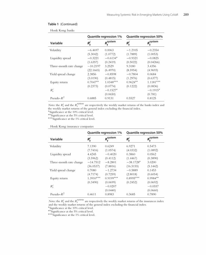
4.1. Quantile RegressionsTable 1 reports quantile regressions results for the 1% and 50% quantile returns of thebanking, insurance, and other financial services industries of the 13 emerging markets.Furthermore,Table 1 reports estimates for the system’s returns in which the General stockmarket index excluding financial services is used to proxy each country’s real economy.Table 1 also reports the pseudo-R2 in order to assess the goodness-of-fit of quantileregressions. This measure has a similar interpretation as the standard R2. The pseudo-R2

is derived using the distances from data points to estimates in each quantile regression ateach point along the Ri

t—distribution. The estimated pseudo-R2 obtained values implythat our estimated models have the appropriate specification.

2 The insurance index is not available for the Czech Republic, Hungary, Poland, Romania, Indonesia, or the Philippines.For these economies we consider only the banking and other financial services industries.

3 Adrian and Brunnermeier (2011) and Bernal et al. (2012) employ an additional control variable to capture the timevariation in the tails of asset returns, the change in credit spread which is defined as the difference between the 10-yearMacrobond BBB corporate bonds rate and the 10-year bond rate. However, this data is not available for any emergingeconomies and therefore we did not include it in our estimations.


Table 1 Quantile regressions.

Mexico: banks

Quantile regression 1% Quantile regression 50%

Variable Rit Rsystemt Rit Rsystemt

Volatility −0.2966 −0.0126 −0.2051 0.0143∗(1.6262) (0.0964) (0.2558) (0.0068)

Liquidity spread 0.3532 0.1594∗ 0.4127 0.0062(0.5677) (0.0543) (0.2473) (0.0089)

Three-month rate change −0.5391 −0.0456 −0.1891 0.0086(1.0722) (0.1339) (0.8211) (0.0419)

Yield spread change −0.4450 −0.0970∗ −0.1960∗ −0.0001(0.9396) (0.0416) (0.0858) (0.0027)

Equity return 0.7625∗∗∗ 1.0729∗∗∗ 0.8168∗∗∗ 1.0941∗∗∗(0.1745) (0.0164) (0.0765) (0.0033)

Rit −0.0777∗∗∗ −0.0818∗∗∗

(0.0089) (0.0026)Pseudo-R2 0.3882 0.9577 0.2669 0.9625

Notes: the Rit and the Rsystem

t are respectively the weekly market returns of the banks index andthe weekly market returns of the general index excluding the financial index.∗Significance at the 10% critical level.∗∗Significance at the 5% critical level.∗∗∗Significance at the 1% critical level.

Mexico: insurance companies



Volatility 1.9518 −0.0005 −0.0115 0.0261(2.1089) (0.2284) (0.0432) (0.0334)

Liquidity spread 3.6105 −0.0699 0.0005 −0.0063(3.3281) (0.1010) (0.0203) (0.0213)

Three-month rate change −1.9659 −0.0309 0.5076 −0.0838(2.6027) (0.1198) (0.3921) (0.0529)

Yield spread change −1.3405 0.0585 −0.0016 0.0004(1.2115) (0.0636) (0.0169) (0.0093)

Equity return 0.4465 1.0133∗∗∗ 0.0165 1.0234∗∗∗(0.3026) (0.0137) (0.0147) (0.0055)

Rit 0.0138 0.0059

(0.0193) (0.0045)Pseudo-R2 0.0935 0.9355 0.2500 0.922


t are respectively the weekly market returns of the insurances indexand the weekly market returns of the general index excluding the financial index.∗Significance at the 10% critical level.∗∗Significance at the 5% critical level.∗∗∗Significance at the 1% critical level.


Table 1 (Continued)

Mexico: financial services



Volatility −0.1950 0.0782 −0.2650 0.0032(1.2309) (0.0726) (0.2729)

Liquidity spread 0.2866 −0.0567 0.0005 0.0004(0.5577) (0.0323) (0.1712)

Three-month rate change −0.3866 0.0483 0.5282 −0.0097(1.4056) (0.0636) (0.3741)

Yield spread change 0.0124 0.0275 −0.0717 0.0006(0.4426) (0.0310) (0.0894)

Equity return 0.7742∗∗∗ 1.1230∗∗∗ 0.7800∗∗∗ 1.1108∗∗∗(0.1917) (0.0110) (0.0588) (0.0012)

Rit −0.1168∗∗∗ −0.1110∗∗∗

(0.0062) (0.0012)Pseudo-R2 0.4663 0.9785 0.3405 0.9807


t are respectively the weekly market returns of the financial servicesindex and the weekly market returns of the general index excluding the financial index.∗Significance at the 10% critical level.∗∗Significance at the 5% critical level.∗∗∗Significance at the 1% critical level.

Czech Republic: banks



Volatility −5.8501∗∗∗ −0.0223 0.0036 0.0475(1.9607) (0.3235) (0.6347) (0.0255)

Liquidity spread 1.9368 1.4582 0.1806 0.0365(3.4615) (0.7674) (1.6295) (0.1107)

Three-month rate change −14.6919∗∗∗ 2.1009 −0.2650 0.0386(3.8920) (1.2612) (1.5385) (0.0780)

Yield spread change −1.1872 0.3350∗∗∗ 0.0464 0.0222(0.8069) (0.1281) (0.2226) (0.0114)

Equity return 1.5970∗∗∗ 1.2104∗∗∗ 0.9701∗∗∗ 1.2029∗∗∗(0.2162) (0.0262) (0.0780) (0.0516)

Rit −0.1909∗∗∗ −0.1923∗∗∗

(0.0195) (0.0041)Pseudo-R2 0.5186 0.9251 0.2179 0.9256




Table 1 (Continued)

Czech Republic: financial services



Volatility −5.5203∗∗∗ −0.2075 −0.1094 0.0444(1.5439) (0.2862) (0.5936) (0.0233)

Liquidity spread −1.0939 0.6498 0.8666 0.0306(4.6569) (0.4293) (1.6452) (0.1343)

Three-month rate change −13.9268∗∗ 1.0989 −1.2100 0.1195(4.8530) (1.1885) (1.4743) (0.0882)

Yield spread change −0.4681 0.1839 −0.0169 0.0244∗(0.6755) (0.1271) (0.2532) (0.0101)

Equity return 1.5445∗∗∗ 1.2310∗∗∗ 0.9655∗∗∗ 1.1979∗∗∗(0.2535) (0.0257) (0.0641) (0.0064)

Rit −0.2204∗∗∗ −0.1966∗∗∗

(0.0226) (0.0049)Pseudo-R2 0.5254 0.9261 0.2150 0.9246



Hungary: banks



Volatility −3.1705∗ −1.0626∗∗ 0.0456 0.0501(1.3976) (0.3612) (0.4189) (0.0436)

Liquidity spread −0.5483 0.2519 −0.0735 −0.0179(1.1452) (0.1653) (0.6613) (0.0510)

Three-month rate change −5.0844∗∗∗ −0.4281 −1.1520 −0.0119(1.3626) (0.2986) (0.7928) (0.0359)

Yield spread change −0.8306∗∗ 0.1934∗∗∗ −0.0718 0.0003(0.2837) (0.0413) (0.0680) (0.0058)

Equity return 1.3542∗∗∗ 1.3826∗∗∗ 1.2896∗∗∗ 1.3078∗∗∗(0.1272) (0.0326) (0.0658) (0.0079)

Rit −0.3380∗∗ −0.3016∗∗

(0.0192) (0.0064)Pseudo-R2 0.6646 0.9074 0.4206 0.9040




Table 1 (Continued)

Hungary: financial services



Volatility −2.3062∗ −1.0564∗∗ 0.0655 0.0312(0.9273) (0.3504) (0.4236) (0.0362)

Liquidity spread −0.0564 0.2182 −0.1577 −0.0027(1.1198) (0.1831) (0.5518) (0.0235)

Three-month rate change −4.8104∗∗∗ −0.4428 −0.9210 −0.0277(1.2297) (0.3441) (0.6408) (0.0236)

Yield spread change −0.6927∗∗ 0.2075∗∗∗ −0.0685 −0.0051(0.2264) (0.0468) (0.0732) (0.0047)

Equity return 1.2871∗∗∗ 1.3787∗∗∗ 1.2561∗∗∗ 1.3249∗∗∗0.1043) (0.0382) (0.0613) (0.0063)

Rit −0.3548∗∗∗ −0.3281∗∗∗

(0.0207) (0.0064)Pseudo-R2 0.6714 0.9066 0.4206 0.9040



Poland: banks



Volatility −1.2853 −0.2600 0.2062 −0.1166(1.2868) (0.4101) (0.2884) (0.0859)

Liquidity spread −0.5227 −0.0073 0.0075 0.0265(0.3872) (0.1033) (0.0977) (0.0234)

Three-month rate change 0.6493 0.0868 −0.0874 −0.1389(0.9271) (0.3243) (0.2030) (0.0747)

Yield spread change 0.4940∗∗∗ −0.0048 −0.0638 −0.0190∗(0.1468) (0.0567) (0.0376) (0.0092)

Equity return 1.2544∗∗∗ 1.6175∗∗∗ 1.0712∗∗∗ 1.6004∗(0.1220) (0.0598) (0.0286) (0.0239)

Rit −0.5941∗∗∗ −0.6181∗∗∗

(0.0400) (0.0233)Pseudo-R2 0.6570 0.8759 0.5645 0.8572




Table 1 (Continued)

Poland: financial services



Volatility −1.6784 −0.5244∗ 0.0468 0.0008(1.1358) (0.2440) (0.2013) (0.0260)

Liquidity spread −0.3985 −0.1169 0.0441 0.0312(0.2802) (0.0707) (0.1044) (0.0201)

Three-month rate change 0.7467 −0.0656 0.0864 −0.0330(0.8109) (0.1889) (0.1945) (0.0271)

Yield spread change 0.5197∗∗∗ 0.0960∗ −0.0607 −0.0173(0.1418) (0.0373) (0.0419) (0.0090)

Equity return 1.1911∗∗∗ 1.7164∗∗∗ 1.0153∗∗∗ 1.7947∗∗∗(0.1360) (0.0470) (0.0270) (0.0173)

Rit −0.7526∗∗∗ −0.8123∗∗∗

(0.0411) (0.0161)Pseudo-R2 0.6948 0.9157 0.5876 0.9178



Romania: banks



Volatility −1.4403 0.3458 −0.6337 0.0361(1.2755) (0.8352) (0.3294) (0.1310)

Liquidity spread −1.8808 0.1307 0.0493 −0.0341(1.0993) (0.3029) (0.3197) (0.0517)

Three-month rate change −1.5584 0.0477 −0.0567 −0.0368(1.8411) (0.3561) (0.4360) (0.0769)

Yield spread change 1.1922∗∗ −0.0019 −0.1094 0.0217(0.3895) (0.1768) (0.1112) (0.231)

Equity return 1.0925∗∗∗ 1.5570∗∗∗ 0.9175∗∗∗ 1.3678∗∗∗(0.1103) (0.0786) (0.0211)

Rit −0.5201∗∗∗ −0.3889∗∗∗

(0.0815) (0.0172)Pseudo-R2 0.6615 0.9271 0.4423 0.8572




Table 1 (Continued)

Romania: financial services



Volatility −1.9274 −0.3478 −0.2637 0.0055(1.1703) (0.2174) (0.3707) (0.0125)

Liquidity spread −0.5855 −0.0976 −0.1592 0.0158(0.9897) (0.0614) (0.2865) (0.0093)


Yield spread change 0.8933∗ −0.0207 −0.0131 0.0010(0.3653) (0.0319) (0.0988) (0.0034)

Equity return 1.2687∗∗∗ 1.5055∗∗∗ 0.9516∗∗∗ 1.5834∗∗∗(0.1963) (0.0329) (0.0434) (0.0124)

Rit −0.4939∗∗∗ −0.5792∗∗∗

(0.0300) (0.0129)Pseudo-R2 0.7551 0.9784 0.5511 0.9578



Turkey: banks



Volatility −3.8876 −0.5620 0.7080 −0.1331(2.5255) (0.8940) (0.7637) (0.3242)


Three-month rate change −0.1054 0.2031 0.5937 0.0374(0.8660) 0.3790) (0.4975) (0.1180)

Yield spread change −0.0525 −0.1306 −0.0927 0.0052(0.3369) (0.0940) (0.1737) (0.0394)

Equity return 1.3065∗∗∗ 1.8485∗∗∗ 1.2452∗∗∗ 1.7585∗∗∗(0.1299) (0.1595) (0.0647) (0.0478)

Rit −0.9109∗∗∗ −0.8017∗∗∗

(0.1172) (0.0385)Pseudo-R2 0.7881 0.8982 0.6994 0.8538




Table 1 (Continued)

Turkey: insurance companies



Volatility −8.3180∗ −1.3265 −3.2190 0.0715(3.8619) (1.5795) (1.9185) (0.8088)



Yield spread change 0.9536 −0.0904 0.0713 −0.0053(0.5683) (0.2223) (0.3438) (0.1550)

Equity return 0.7338∗∗∗ 0.7746∗∗∗ 0.8917∗∗∗ 0.7011∗∗∗(0.2062) (0.1452) (0.0824) (0.0613)

Rit 0.0230 0.0396

(0.0764) (0.0462Pseudo-R2 0.6376 0.7468 0.2420 0.5963



Turkey: financial services



Volatility −3.3219 −0.8118∗ −0.1035 −0.0120(2.0211) (0.3303) (0.8051) (0.0596)


Three-month rate change 0.5409 0.2051 0.5931 0.0060(0.6783) (0.1280) (0.3497) (0.0227)

Yield spread change 0.2828 0.0835∗∗ 0.0833 0.0066(0.1912) (0.0298) (0.1266) (0.0135)

Equity return 1.2325∗∗∗ 2.2176∗∗∗ 1.2195∗∗∗ 2.0792∗∗∗(0.0885) (0.0610) (0.0486) (0.0135)

Rit −1.2002∗∗∗ −1.0770∗∗∗

(0.0491) (0.0124)Pseudo-R2 0.8425 0.9652 0.7528 0.9544




Table 1 (Continued)

Honk Kong: banks



Volatility −6.4697 0.0063 −1.2105 −0.2354(5.3042) (1.0772) (1.7889) (1.0053)

Liquidity spread −0.3221 −0.6134∗ −0.9321 −0.0825(1.6357) (0.2419) (0.5022) (0.04266)

Three-month rate change −10.2197 3.2529 9.3180 3.4356(22.1665) (6.4970) (8.5954) (4.9693)

Yield spread change 2.3856 −0.8598 −0.7804 0.0684(3.0190) (0.4815) (1.2976) (0.6377)

Equity return 0.7047∗∗ 1.0348∗∗∗ 0.9624∗∗ 1.1181∗∗∗(0.2373) (0.0774) (0.1222) (0.0836)

Rit −0.1527∗ −0.1915∗

(0.0650) (0.781)Pseudo-R2 0.6885 0.9131 0.5527 0.8125



Honk Kong: insurance companies



Volatility 7.1390 0.6249 6.9271 0.5473(7.7416) (1.0574) (4.0332) (1.0892)

Liquidity spread 4.4245 −0.4020 0.3860 0.0562(3.5962) (0.4112) (1.4467) (0.3890)

Three-month rate change −14.7512 −8.2801 −38.1728∗ 3.0200(36.0537) (7.8816) (16.5155) (5.1442)


Equity return 1.3910∗∗∗ 0.9199∗∗∗ 0.8995∗∗∗ 0.9984∗∗(0.3490) (0.0699) (0.2452) (0.0692)

Rit −0.0207 −0.0557

(0.0440) (0.0660)Pseudo-R2 0.4611 0.8983 0.3685 0.7890




Table 1 (Continued)

Honk Kong: financial services



Volatility −5.5107 −0.1013 −0.4319 −0.0073(3.3442) (0.0672) (1.9190) (0.0519)

Liquidity spread 1.0699 −0.0083 0.0454 −0.0010(1.2435) (0.0321) (0.6133) (0.0222)

Three-month rate change −0.0742 −0.1692 −7.6256 −0.0580(8.8936) (0.3755) (7.7663) (0.2857)

Yield spread change 0.6623 0.0767 0.2261 0.0340(1.7609) (0.0440) (1.1742) (0.0397)

Equity return 1.0069∗∗∗ 1.5387∗∗∗ 1.0832∗∗∗ 1.5465∗∗∗(0.1402) (0.0180) (0.0867) (0.0146)

Rit −0.5413∗∗∗ −0.5456∗∗∗

(0.0156) (0.0148)Pseudo-R2 0.7615 0.9936 0.6996 0.9859



Indonesia: banks



Volatility −3.2923∗∗ −0.2489 0.4656 0.0062(1.2000) (0.1444) (0.2754) (0.105)

Liquidity spread 0.4887 0.0336 −0.0232 0.0047(0.3760) (0.0437) (0.0994) (0.0066)

Three-month rate change 0.3704 −0.1826 −0.8251 −0.0154(1.6461) (0.1548) (0.9483) (0.0300)

Yield spread change −0.2493 −0.0126 −0.0146 0.0060∗(0.2059) (0.0290) (0.0511) (0.0028)

Equity return 0.9975∗∗∗ 1.3322∗∗∗ 1.0564∗∗∗ 1.3838∗∗∗(0.011) (0.0279) (0.0286) (0.0066)

Rit −0.3565∗∗∗ −0.3760∗∗∗

(0.0168) (0.0058)Pseudo-R2 0.6578 0.9728 0.5336 0.9637




Table 1 (Continued)

Indonesia: financial services



Volatility −3.2244∗∗ −0.1314 0.3926 0.0056(1.0480) (0.1109) (0.2370) (0.0039)

Liquidity spread 0.1384 0.0665∗∗ −0.0099 0.0005(0.3664) (0.0254) (0.0967) (0.0038)

Three-month rate change 0.2979 −0.1401 −0.8276 −0.0057(1.6392) (0.0863) (0.0509) (0.0219)

Yield spread change −0.0576 −0.0257 −0.0149 0.0008(0.1835) (0.0183) (0.0486) (0.0008)

Equity return 0.9703∗∗∗ 1.3796∗∗∗ 1.0304∗∗∗ 1.4050∗∗∗(0.0881) (0.0160) (0.0266) (0.0019)

Rit −0.3826∗∗∗ −0.4051∗∗∗

(0.0110) (0.0019)Pseudo-R2 0.6724 0.9811 0.5436 0.9792

Notes:The Rit and the Rsystem


Korea: banks



Volatility −4.2649∗∗∗ −0.0725 −0.3687 −0.0689(1.2408) (0.1636) (0.4145) (0.0410)

Liquidity spread −10.1465∗∗∗ 0.0598 −0.9035 0.1287(1.9950) (0.2721) (1.1486) (0.0067)


Yield spread change 0.8920∗ 0.0444 0.3624 −0.0023(0.4357) (0.0825) (0.2454) (0.0140)

Equity return 0.8214∗∗∗ 1.1502∗∗∗ 1.0683∗∗∗ 1.1384∗∗∗(1.1298) (0.0160) (0.1017) (0.0065)

Rit −0.1536∗∗∗ −0.1413∗∗∗

(0.0110) (0.0062)Pseudo-R2 0.5797 0.9610 0.3132 0.9349


t are respectively the weekly market returns of the banks index and theweekly market returns of the general index excluding the financial index.∗Significance at the 10% critical level.∗∗Significance at the 5% critical level.∗∗∗Significance at the 1% critical level.


Table 1 (Continued)

Korea: insurance companies



Volatility 1.7094 −0.6666 0.3917 0.0381(2.4170) (0.3524) (0.7364) (0.0563)

Liquidity spread −1.8349 −0.0824 −2.4150 0.0722(4.5279) (0.3308) (1.6430) (0.1544)


Yield spread change 1.0504 0.0381 0.2667 −0.0264(1.4071) (0.0972) (0.2748) (0.0317)

Equity return 1.1320∗∗∗ 1.0156∗∗∗ 0.7525∗∗∗ 1.0244∗∗∗(1.4071) (0.0272) (0.0662) (0.0131)

Rit −0.0573∗∗∗ −0.0500∗∗∗

(0.0231) (0.0073)Pseudo-R2 0.4840 0.9152 0.2324



Korea: financial services



Volatility −4.4326∗ 0.1269 0.1283 −0.0012(2.0750) (0.0650) (0.3841) (0.0071)

Liquidity spread 0.9476 −0.3003 −0.2612 0.0155(2.7630) (0.2117) (0.8166) (0.0140)

Three-month rate change 12.8915 −0.1132 3.1132 0.0816∗∗(11.1145) (0.3144) (2.1022) (0.0303)

Yield spread change −1.0793∗ 0.0168 0.0736 −0.0013(0.5259) (0.0392) (0.1461) (0.0034)

Equity return 0.8221∗∗∗ 1.2099∗∗ 1.0387∗∗∗ 1.2033∗∗∗(0.1560) (0.0089) (0.529) (0.0035)

Rit −0.2165∗∗∗ −0.2033∗∗∗

(0.0106) (0.0034)Pseudo-R2 0.6058 0.9823 0.4305 0.9798




Table 1 (Continued)

Malaysia: banks



Volatility −2.2497∗ −0.2664∗∗∗ 0.0831 0.0085(0.9671) (0.0773) (0.2538) (0.0234)



Yield spread change 0.1223 −0.0524 0.1034 0.0112(0.5612) (0.0317) (0.0968) (0.0104)

Equity return 1.0876∗∗∗ 1.2730∗∗∗ 1.0047∗∗∗ 1.2638∗∗∗(0.1172) (0.0117) (0.0362) (0.0075)

Rit −0.3016∗∗∗ −0.2867∗∗∗

(0.0100) (0.0061)Pseudo-R2 0.6848 0.9702 0.5161 0.9482



Malaysia: insurance companies



Volatility −11.3252∗∗∗ −0.9666∗∗∗ 0.0472 −0.0461(3.9085) (0.2894) (0.4699) (0.1323)

Liquidity spread 1.2972 −0.1772∗ 0.2092 −0.0100(1.7761) (0.0853) (0.2984) (0.0418)

Three-month rate change 6.9709 −0.9004 −0.5689 0.0334(9.5411) (0.6551) (1.7372) (0.2633)

Yield spread change −1.0521 −0.2167∗ −0.0502 −0.0313(1.0338) (0.1031) (0.2231) (0.0377)

Equity return 0.8019∗ 0.9673∗∗∗ 0.6289∗∗∗ 0.9585∗∗∗(0.4018) (0.0249) (0.0972) (0.0142)

Rit −0.0582∗∗∗ 0.0068

(0.0172) (0.0104)Pseudo-R2 0.2640 0.9098 0.1263 0.8239




Table 1 (Continued)

Malaysia: financial services



Volatility −1.2280 −0.0249 0.0009 0.0020(0.9452) (0.0301) (0.2953) (0.0031)

Liquidity spread −0.6430 −0.0147 0.0602 −0.0007(0.4447) (0.0116) (0.1147) (0.0012)



Equity return 1.2681∗∗∗ 1.3351∗∗∗ 1.0936∗∗∗ 1.3547∗∗∗(0.1248) (0.0072) (0.0240) (0.034)

Rit −0.3365∗∗∗ −0.3548∗∗∗

(0.0062) (0.0034)Pseudo-R2 0.7323 0.9930 0.5879 0.9911



Philippines: banks



Volatility −2.8536∗ 0.0330 −0.3156 −0.0716(1.2027) (0.3819) (0/2731) (0.0563)

Liquidity spread 0.1106 −0.0381 −0.0161 −0.0250(0.2020) (0.0621) (0.0715) (0.0186)

Three-month rate change −0.9939 0.1973 −0.1596 −0.0173(0.5172) (0.2682) (0.3305) (0.0440)

Yield spread change −0.0411 −0.0964∗ −0.0843 −0.0142(0.1129) (0.0435) (0.0479) (0.0124)

Equity return 0.8156∗∗∗ 1.2403∗∗∗ 0.9278∗∗∗ 1.2280∗∗∗(0.1129) (0.0544) (0.0317) (0.0151)

Rit −0.3201∗∗∗ −0.2814∗∗∗

(0.0499) (0.0141)Pseudo-R2 0.6245 0.8835 0.4605 0.8321




Table 1 (Continued)

Philippines: financial services



Volatility −1.7896 −0.1513 −0.0743 0.0011(1.1239) (0.1286) (0.2459) (0.0176)

Liquidity spread 0.5203∗∗∗ 0.0311 −0.0072 0.0063(0.1414) (0.0446) (0.0467) (0.0053)

Three-month rate change −0.9265 −0.0778 0.0446 −0.0079(0.8356) (0.0720) (0.2432) (0.0261)

Yield spread change 0.1463 −0.0896∗∗ −0.0016 0.0040(0.0904) (0.0289) (0.0428) (0.0043)

Equity return 0.9154∗∗∗ 1.4566∗∗∗ 1.0753∗∗∗ 1.4828∗∗∗(0.0745) (0.0225) (0.0307) (0.0225)

Rit −0.4879∗∗∗ −0.4840∗∗∗

(0.0263) (0.0221)Pseudo-R2 0.7094 0.9491 0.5920 0.9419



Singapore: banks



Volatility −5.6314∗∗∗ −1.1196∗∗ 0.5068 0.2346∗∗∗(1.3706) (0.2838) (0.3116) (0.0707)



Yield spread change 0.8717∗ 0.0202 0.0656 0.0210(0.3481) (0.0983) (0.0676) (0.0186)

Equity return 1.4728∗ 1.2406∗∗∗ 1.1272∗∗∗ 1.2935∗∗∗(0.1460) (0.0335) (0.0469) (0.0192)

Rit −0.3135∗∗∗ −0.3203∗∗∗

(0.0231) (0.0175)Pseudo-R2 0.6262 0.8732 0.4706 0.8339




Table 1 (Continued)

Singapore: insurance companies



Volatility −9.6197∗∗ −2.5613∗∗ −0.0483 0.0680(3.6951) (0.7753) (0.4554) (0.0799)

Liquidity spread 1.6195 −0.1287 −0.4837 0.0530(1.2065) (0.5499) (0.3491) (0.0721)

Three-month rate change 6.7470 −1.1680 0.7206 0.7253∗∗(4.0473) (0.8008) (1.1381) (0.2621)

Yield spread change −0.5644 −0.0406 0.0874 −0.0325(0.5392) (0.1594) (0.1016) (0.0282)

Equity return 0.2743 0.9620∗∗∗ 0.3989∗∗∗ 0.9472∗∗∗(0.3033) (0.0576) (0.0578) (0.0161)

Rit −0.0793∗ −0.0336∗∗

(0.0332) (0.0116)Pseudo-R2 0.3160 0.7606 0.0757 0.7224



Singapore: financial services



Volatility −5.0329∗ −0.8242∗∗∗ −0.1750 −0.0002(2.1215) (0.2304) (0.1800) (0.0090)

Liquidity spread −3.6533∗ −0.7685 −0.0495 −0.0079(1.8492) (0.4114) (0.1110) (0.0113)

Three-month rate change −1.6315 −0.5365 −1.4013∗ −0.0600(2.4357) (0.4904) (0.6557) (0.0321)


Equity return 1.2696∗∗∗ 1.5332∗∗∗ 1.1139∗∗∗ 1.5856∗∗∗(0.1125) (0.0618) (0.0287) (0.0082)

Rit −0.5348∗∗∗ −0.5850∗∗∗

(0.0581) (0.0085)Pseudo-R2 0.6654 0.9225 0.6163 0.9563




Table 1 (Continued)

Thailand: banks



Volatility −0.4978 0.0789∗ 0.2956 0.0181(1.1203) (0.0401) (0.3679) (0.0173)

Liquidity spread 2.6328∗ 0.1177 −0.5904 −0.0009(1.1124) (0.0780) (0.5078) (0.0356)



Equity return 1.0958∗∗∗ 1.3149∗∗∗ 1.0352∗∗∗ 1.3082∗∗∗(0.1402) (0.0103) (0.0305) (0.0058)

Rit −0.3149∗∗∗ −0.3067∗∗∗

(0.0099) (0.0046)Pseudo-R2 0.7052 0.9819 0.5491 0.9646



Thailand: insurance companies



Volatility −3.2089 −0.6079 −0.0301 0.0768(2.6942) (0.3370) (0.5916) (0.1163)

Liquidity spread −10.1392∗∗ 0.6455 −0.3401 0.2406(3.8848) (0.4466) (0.5176) (0.1736)

Three-month rate change −21.1113∗ −1.2609 0.8836 −0.7231(9.2554) (−1.5294) (1.8312) (0.5840)

Yield spread change 1.8403∗ 0.0261 0.1847 −0.0071(0.8385) (0.1041) (0.1147) (0.0335)

Equity return 0.6952∗∗∗ 0.8895∗∗∗ 0.2132 0.9803∗∗∗(0.2022) (0.0470) (0.1134) (0.0131)

Rit 0.0138 0.0018

(0.0144) (0.0069)Pseudo-R2 0.4416 0.8977 0.0127 0.8215




Table 1 (Continued)

Thailand: financial services



Volatility −0.7821 −0.0604 −0.0618 0.0027(0.8500) (0.0561) (0.3406) (0.0032)

Liquidity spread 0.9903 0.0372 −0.7055 0.0153(1.0879) (0.0804) (0.4923) (0.0083)

Three-month rate change −0.5807 −0.0700 2.5191 0.0045(4.0308) (0.1839) (1.7136) (0.0217)


Equity return 1.1214∗∗∗ 1.3569∗∗∗ 1.0626∗∗∗ 1.3297∗∗∗(0.1282) (0.0140) (0.0347) (0.7921)

Rit −0.3470∗∗∗ −0.3299∗∗∗

(0.0101) (0.0034)Pseudo-R2 0.7495 0.9856 0.5662 0.9801



Results for the Mexican banking industry show that equity returns have a positiveimpact on the 1% quantile returns of the banking index. With respect to the bankingindex at 50% (normal state), we observe that equity returns still influence its returnbut in addition volatility also has a positive effect. Turning now to the General Indexex Financials 1% quantile returns, we note that liquidity spread and equity returns arestatistically significant with a positive sign, whereas yield spread change and bank indextotal return are statistically significant with a negative sign. With respect to the 50%quantile returns for the General Index ex Financials, volatility and equity returns havea positive influence and bank index total return has a negative impact. The situation ofthe Mexican insurance industry is somehow weaker since the only statistically significantcontrol variable is the equity return for the 1% and 50% quantile returns for the GeneralIndex ex Financials. Finally, our estimates for other financial services in Mexico showthat both 1% and 50% quantile returns are positively impacted by equity returns for theGeneral Index ex Financials, whereas the insurance index total return has no statisticallysignificant impact on the system variable.

The evidence for the four Central and Eastern European countries relies only on thebanking industry and the other financial services industry since no insurance index isavailable. Looking at the banking industry of the Czech Republic, we see that the 1%quantile returns of the banking index are influenced positively by the three-month rate


change and the equity returns and negatively by volatility. In the case of the banking indexat the 50% quantile returns, only the equity return has a statistically significant impact.For the case of the 1% and 50% quantile returns of the General Index ex Financials, theyield spread change and equity returns enter positively and the bank index total returnsnegatively and equity returns positively and bank index returns negatively, respectively.The banking index of Hungary, Poland, and Romania exhibits very similar patterns withrespect to the variables that influence the banking index and the General Index exFinancials at the 1% and 50% quantile returns, although in the case of Poland andRomania the three-month rate change is not statistically significant.

Looking at the financial services industry for the Czech Republic, our results indicatethat the financial services 1% quantile returns are negatively related to volatility and thethree-month rate change and positively to equity returns. The 50% quantile returns areonly positively related to equity returns.The General Index ex Financials 1% and 50% arepositively influenced by equity returns and negatively by the financial index total return,whereas in addition the 50% quantile returns are influenced by the yield spread change.Hungary’s 1% and 50% quantile returns for the financial services index are similar to thoseof the Czech Republic, but in addition volatility is also statistical by significant with anegative sign. The same holds for the 1% and 50% for the General Index ex Financials.Poland and Romania exhibit minor differences from the results obtained for the CzechRepublic and Hungary since the volatility variable has no influence on the 1% and 50%for the financial services index. The results for the 1% and 50% quantile returns of theGeneral Index ex Financials show no significant statistically significant results.

Results for the Turkish banking industry indicate that only equity returns positivelyinfluence the bank index at the 1% and 50% quantile returns and the same evidence holdsfor both estimated quantiles for the General Index ex Financials.Turning our attention tothe insurance industry, we observe that at the 1% quantile returns of the insurance index,volatility enters significantly with a negative sign and the equity returns affect this indexpositively. In the 50% quantile returns, only the equity returns have a positive impact.In the case of the General Index ex Financials, the equity returns are the only variablethat influences in a positive way at both the 1% and 50% quantile returns. Finally, ourestimates for the other financial services in Turkey indicate that both the 1% and 50%quantile returns for the financial services index are negatively influenced by the equityreturns. Concerning the General Index ex Financials, the volatility and the financialservices total returns negatively influence and yield spread change and equity returnspositively influence at the 1% quantile returns, whereas at the 50% quantile returns,equity returns have a positive impact and the financial services total returns influence ina negative manner.

Finally, we discuss the evidence from Southeast Asia. For the case of Indonesia andthe Philippines, we only consider the effects of the banking and other financial servicesindustries. For the case of the banking sector in Hong Kong,we observe that for both the


1% and 50% quantile returns the equity returns positively influence the banking index.For both the 1% and the 50% of the General Index ex Financials, the equity returns have apositive impact and the liquidity spread and the banking sector total return have a negativeimpact. In addition for the 1% quantile returns there is a negative effect by liquidity spread.Similar results were obtained for Indonesia, Korea, Malaysia, the Philippines, Singapore,and Thailand. Furthermore, in these markets the liquidity spread change and volatilityalso play an important role.

The results for the insurance industry are summarized as follows. In Hong Kong, forboth the 1% and 50% quantile returns, equity returns positively affect the insurance indexand for the latter case, the index is also influenced negatively by the three-month ratechange. For the 1% and 50% quantile returns for the General Index ex Financials index,only the equity returns positively affect the insurance index.The results for the insuranceindustry in Korea, Malaysia, Singapore, and Thailand are similar. In Korea, Malaysia, andSingapore,the insurance index total return enters significantly in the 1% and 50% quantilereturns of the General Index ex Financials.

Finally, our estimates for other financial services in Hong Kong at the 1% and 50%quantile returns of the insurance index are influenced positively by the equity returns.For the General Index ex Financials both at the 1% and 50% quantile returns, the equityreturns have a positive impact and the financial services total return has a negative effect.Similar results hold for Malaysia and Thailand. In addition, for the case of Indone-sia, Korea, the Philippines, and Singapore, the liquidity spread has a positive impact atthe 1% quantile returns, whereas the coefficient of volatility is negative and statisticallysignificant.

4.2. �CôVaR EstimatesIn this section,we present and discuss the �CôVaR estimates based on our presentation inSection 3.We define that a �CôVaR with a value of zero implies that none of the threefinancial industries contributes to the systemic risk. Therefore, if the value is differentfrom zero, we then consider the case that the financial industry which has the largerabsolute estimate of �CôVaR is taken to be the sector that contributes relatively themost to systemic risk in periods of distress.

In Table 2, we report descriptive statistics of the estimated �CôVaR. We observethat for Mexico, the Czech Republic, Hungary, Romania, Hong Kong, Indonesia, thePhilippines, and Thailand, the absolute value of the estimated �CôVaR conditional tothe banking sector is larger than the corresponding values for the insurance and otherfinancial services industries. This finding suggests that when a distress situation occurredin the banking industry, it will increase the value of theVaR in those emerging marketsas a whole compared with the normal state. Looking at the cases of Poland, Turkey,Korea, and Singapore, it is documented that the estimated �CôVaR conditional to thefinancial services industry has the larger absolute value and therefore it is the segment of


Table 2 �CôVaR estimates.

Mexico

1996–2013 1996–2007 2008–2013

Mean Standarddeviation



�CoVaR banks −0.227 0.137 0.005 0.093 −0.165 0.192�CoVaR insurances −0.003 0.030 0.006 0.080 −0.014 0.120�CoVaR financial

services0.002 0.025 −0.033 0.107 0.065 0.218

Czech Republic

1999–2013 1999–2007 2008–2013




�CoVaR banks 1.390 0.602 −0.024 0.223 1.155 0.882�CoVaR financial

services0.838 0.691 0.619 0.296 1.208 0.854

Hungary

1999–2013 1999–2007 2008–2013




�CoVaR banks −0.814 1.028 −0.498 0.372 −2.038 0.773�CoVaR financial

services−0.610 0.988 −0.231 0.354 −1.583 0.563

Poland

1999–2013 1999–2007 2008–2013




�CoVaR banks 0.084 0.857 0.201 0.471 0.020 0.525�CoVaR financial

services−0.343 0.949 0.371 0.939 0.984 1.512


Table 2 (Continued)

Romania

1996–2013 1996–2007 2008–2013




�CoVaR banks 2.429 1.543 0.044 0.444 2.523 1.593�CoVaR financial

services1.767 1.332 0.084 0.849 1.605 1.143

Turkey

1996–2013 1996–2007 2008–2013




�CoVaR banks −0.060 0.575 −0.091 0.631 −0.012 0.403�CoVaR insurances 0.043 0.415 0.020 0.432 0.008 0.291�CoVaR financial

services−0.431 0.147 −0.139 0.061 −0.415 0.147

Hong Kong

1996–2013 1996–2007 2008–2013




�CoVaR banks −1.695 0.247 −1.203 0.401 −1.895 0.247�CoVaR insurances −0.008 0.268 −0.032 0.135 0.005 0.273�CoVaR financial

services0.004 0.130 0.015 0.090 1.543 1.145

Indonesia

1998–2013 1998–2007 2008–2013





services1.197 0.537 −0.191 0.364 1.334 0.807


Table 2 (Continued)

Korea

1996–2013 1996–2007 2008–2013




�CoVaR banks 0.774 0.574 −0.638 0.360 0.376 0.365�CoVaR insurances −0.005 0.159 0.006 0.151 −0.905 0.441�CoVaR financial

services1.163 0.472 0.800 0.527 1.294 0.538

Malaysia

1996–2013 1996–2007 2008–2013




�CoVaR banks 0.259 0.215 0.003 0.164 0.677 0.369�CoVaR insurances −0.766 0.213 −0.308 0.381 −2.019 0.332�CoVaR financial

services−0.004 0.172 0.004 0.192 −0.0004 0.017

Philippines

1998–2013 1998–2007 2008–2013





services−0.482 0.352 1.050 0.454 −0.123 0.185

Singapore

1998–2013 1998–2007 2008–2013




�CoVaR banks −0.256 0.517 1.240 0.704 1.517 0.600�CoVaR insurances −1.184 0.590 −2.222 0.964 1.449 0.683�CoVaR financial

services2.159 1.995 1.444 1.189 2.271 0.730


Table 2 (Continued)

Thailand

1996–2013 1996–2007 2008–2013




�CoVaR banks −0.221 0.189 −0.207 0.201 0.181 0.281�CoVaR insurances −0.003 0.388 0.002 0.202 0.0057 0.098�CoVaR financial

services−0.000 0.0491 −0.105 0.090 0.008 0.154

Notes: all the figures above are in percentages.

the financial sector that contributes most to the systemic risk in these emerging markets.Finally, in Malaysia, the absolute value of the estimated �CôVaR conditional to theinsurance industry has the larger absolute value which means that when this industry isin distress will contribute most to the systemic risk.

An additional interesting result we can derive from the results in Table 2 is thatwhen we split the full sample into two periods, before and after the financial crisis withthe year 2008 as the break point, then we note that the absolute values of the estimated�CôVaR for all cases in the period prior to the financial crisis are smaller compared withthose obtained for the post-crisis period.This finding provides further evidence that thebanking, insurance, and other financial services, when in distress, contribute more to thesystemic risk as the financial crisis moves into full swing.

5. SUMMARY AND CONCLUDING REMARKS

The recent financial crisis led to the understanding that financial intermediary distressdocumented in extreme (tail) events tend to spill over to financial institutions, financialindustries and through them to the whole economy. It was also made clear that suchspillovers are the results of an increase in the risk-appetite of banks, insurances, and otherfinancial services, either individually or at the industry level. Another important aspect ofthese negative effects is the need for a new regulatory framework that is currently underdevelopment within the context of Basle III in order to embody the main factors ofsystemic risk. Following the failure of the micro-prudential regulatory framework, thereis now a shift to the development of macro-prudential regulations.

In this chapter, we adopt �CoVaR, a recent econometric methodology developedby Adrian and Brunnermeier (2011). This is a parsimonious measure of systemic riskthat complements measures designed for individual financial institutions and extends risk


measurement to allow for a macro-prudential approach.We implement this new measureof systemic risk on selected countries from three regions of emerging markets, namely,Latin America, Central and Eastern Europe, and Southeast Asia. Although recent studiesinvestigate many aspects of the financial crisis in relation to developed economies, lessresearch has been done with respect to emerging economies. Following Bernal et al.(2012), we do not study systemic risk in the context of individual financial institutions.We consider the contribution of the banking, insurance, and other financial servicesindustries that may be in distress to the systemic risk.The �CoVaR analysis allows us toinvestigate the additional level of risk that the economy as a whole faces when at leastone of the financial sectors is in distress.

We use weekly data for the period December 1995–February 2013 for Mexico,the Czech Republic, Hungary, Poland, Romania,Turkey, Hong Kong, Indonesia, Korea,Malaysia, the Philippines, Singapore, and Thailand. The main findings, based on estima-tion of 1% and 50% quantile regressions, show that equity returns are a key determinantin triggering systemic risk episodes. There is also evidence that volatility of the generalindex ex financials (system variable), liquidity spread, the three-month rate change, andyield spread have an effect although weaker. Furthermore, we show that for Mexico,the Czech Republic, Hungary, Romania, Hong Kong, Indonesia, the Philippines, andThailand, it is the banking sector that contributes mostly to the systemic risk. In Malaysia,the insurance industry contributes most to the systemic risk, whereas in Poland,Turkey,Korea, and Singapore the highest percentage contribution to systemic risk is due to theother financial services. Finally, based on the results of �CoVaR estimates before andafter 2008, it is observed for all emerging markets that the contribution of each financialindustry to systemic risk increased after the unfolding of the crisis.

Our results are of interest to regulators since it is shown that the different financialindustries have an important and negative impact on the economy as a whole. It isemphasized that regulatory authorities should be able to identify the different segmentsof the financial sector of the economy which represent different risks for the system.Therefore, there is a need for regulatory provisions to reduce the risk on the wholeeconomy emanating from these financial industries being in distress.

ACKNOWLEDGMENTSKouretas acknowledges financial support from a Marie Curie Transfer of Knowledge Fellowship of theEuropean Community’s Sixth Framework Programme under Contract No. MTKD-CT-014288, as well asfrom the Research Committee of the University of Crete under Research Grant #2257. We thank SteliosBekiros, Manthos Delis, Dimitris Georgoutsos Jean-Yves Gnabo, and Christos Tsoumas for many helpfulcomments and discussions. Theodoros Bratis, Elpianna Emmanouilidi, and Evangelos Salachas providedsuperb research assistance.We also thank Marcus Brunnermeier and Jean-Yves Gnabo for providing us withthe STATA codes for estimating CoVaR. The usual caveat applies.


REFERENCESAcharya,V.V., Richardson, M., 2009. Restoring Financial Stability: how to Repair a Failed System. John

Wiley and Sons, NewYork.Acharya,V.V., Pedersen, L.H., Philippon, T., Richardson, M.P., 2010. Measuring systemic risk. New York

University,Working Paper.Acharya,V.V., Engle, R., Richardson, M., 2012. Capital shortfall: a new approach to ranking and regulating

systemic risk. American Economic Review 102, 59–64.Adrian,T., Brunnermeier, M.K., 2011. CoVaR, NBER Working Paper No, 17454.Agrippino, S.M., 2009. Measuring risk contagion and interdependence, Bocconi University, Department of

Economics,Working Paper.Alessi, L., Detken, C., 2009. Real time early warning indicators for costly asset price boom/bust cycles: a

role for global liquidity, European Central Bank Working Paper 1039.Alfaro, R., Drehmann, M., 2009. Macro stress tests and crises: what can we learn? BIS Quarterly

Review, 29–41 December.Arnold, B., Borio, C., Ellis, L., Moshirian, F., 2012. Systemic risk, macroprudential policy frame-

works, monitoring financial systems and the evolution of capital adequacy. Journal of Banking andFinance 36, 3125–3132.

Barth, J., Caprio, G., 2006. Rethinking Bank Regulation:Till Angels Govern. Cambridge University Press,Cambridge.

Bernal, O., Guilmin, G., Gnabo, J-Y., 2012. Assessing the Contribution of Banks, Insurances and OtherFinancial Services to Systemic Risk, Mimeo.

Bisias, D., Flood, M., Lo,A.W.,Valavanis, S., 2012. A survey of systemic risk analytics. U.S., Department ofTreasury, Office of Financial Research,Working Paper No 1.

Bjarnadottir, F., 2012. Implementation of CoVaR. A measure for systemic risk. KTH Royal Institute ofTechnology,Working Paper.

Borio, C., Drehmann, M., 2009. Assessing the risk of banking crisis-revisited. BIS Quartely Review, 29–46.Borio, C., Drehmann, M.,Tsatsaronis, K., forthcoming. Stress-testing, macro-stress tests: does it live up to

expectations? Journal of Financial Stability.Borio, C., Lowe, P., 2002. Assessing the risk of banking crisis. BIS Quartely Review, 43–54.Brownlees, C.T., Engle, R.F., 2012.Volatility, correlation and tails for systemic risk measurement. NewYork

University,Working Paper.Brunnermeier, M., Pedersen, L.H., 2009. Market liquidity and funding liquidity. Review of Financial

Studies 22, 2201–2238.Cerutti, E., Claessens, S., McGuire, P., 2011. Systemic risks in global banking: what available data can tell us

and what more data are needed? IMF Working Paper 11/222.Chan-Lau, J.A., 2008. Default risk codependence in the global financial system: was the bear stearns bailout

justified? IMF and Tufts University,Working Paper.Demirguc-Kunt,A., Kane, E., Laeven, L., 2009. Deposit Insurance Around the World: issues of Design and

Implementation. MIT Press, Cambridge Mass.Demirguc-Kunt, A., Detragiache, E., 2011. Basel core principles and bank soundness: does compliance

matter? Journal of Financial Stability 7, 179–190.Forbes,K.,Rigobon,R.,2001. Measuring contagion:conceptual and empirical issues. In:Claasens,S.,Forbes,

K. (Eds.), International Financial Contagion. Kluwer Academic Publishers, Boston, pp. 43–66.Gauthier, C., Lehar,A., Souissi, M., 2012. Macroprudential capital requirements and systemic risk. Journal

of Financial Intermediation 21, 594–618.Giesecke, K., Kim, B., 2011. Risk analysis of collateralized debt obligations. Operation Research 59, 32–49.Girardi,G.,Ergün,T.,2013. Systemic risk measurement:multivariate GARCH estimation of CoVaR. Journal

of Banking and Finance 37, 3169–3180.Goodhart, C., 2006. A framework for assessing financial stability? Journal of Banking and

Finance 30, 3415–3422.Goodhart, C., Sunirand, P., Tsomocos, D., 2005. A risk assessment model for banks. Annals of

Finance 1, 197–224.

http://refhub.elsevier.com/B978-0-12-411549-1.00012-0/h0005



























































































































































































Goodhart, C., Sunirand, P., Tsomocos, D., 2006. A model to analyze financial fragility. Economic The-ory 27, 107–142.

Group of Ten, 2001. Report on consolidation in the financial sector. Bank for International Settlements,Basel, Switzerland.

Huang, X., Zhou, H., Zhu, H., 2009. A framework for assessing the systemic risk of major financial institu-tions. Journal of Banking and Finance 33, 2036–2049.

Jorion, P., 2007. Value at Risk: the New Benchmark for Managing Financial Risk, 3rd ed. McGraw-Hill,NewYork.

Khandani,A.E., Kim,A.J., Lo,A.W., 2010. Consumer credit risk models via machine-learning algorithms.Journal of Banking and Finance 34, 2767–2787.

Klomp, J., de Haan, J., 2012. Banking risk and regulation: does one size fit all? Journal of Banking andFinance 36, 3197–3212.

Koenker, R., 2005. Quantile Regression. Cambridge University Press, Cambridge.Koenker, R., Basset, G.W., 1978. Regression quantiles. Econometrica 46, 33–50.Lehar, A., 2005. Measuring systemic risk: a risk management approach. Journal of Banking and

Finance 29, 2577–2603.Levine, R., 1997. Financial development and economic growth: views and agenda. Journal of Economic

Literature 32, 668–726.Lopez-Espinoza, G., Moreno, A., Rubia, A., Valderrama, L., 2012a. Systemic risk and asymmetric responses

in the financial industry, IMF Working Paper.Lopez-Espinoza,G.,Moreno,A.,Rubia,A.,Valderrama,L.,2012. Short-term wholesale funding and systemic

risk: a global CoVaR approach. Journal of Banking and Finance 36, 3150–3162.Moreno, M.R., Peña, J.J., 2013. Systemic risk measures: the simpler the better? Journal of Banking and

Finance 37, 1817–1831.Pritsker, M., 2000. The channels for financial contagion. In: Claessens, S., Forbes, K. (Eds.), International

Financial Contagion. Kluwer Academic Publishers, Boston.Reinhart, C.M., Rogoff, K.S., 2009. This Time is Different: Eight Centuries of Financial Folly. Princeton

University Press, Princeton.Roengpitya, R., Rungcharoenkitkul, P., 2011. Measuring systemic risk and financial linkages in the Thai

banking system, Bank of Thailand Working Paper.Segoviano, M.A., Goodhart, C., 2009. Banking stability measures, IMF Working Paper.Stein, J.C., 2010. Securitization, shadow banking and financial fragility. Dedalus 139, 41–51.Sylvain, B., Colletaz, G., Hurlin, C., Pérignon, C., 2012. A theoretical and empirical comparison of systemic

risk measures, Mimeo.Wong,A.,Fong,T.,2010.An analysis of the interconnectivity among theAsia-Pacific economies,Hong Kong

Monetary Authority Working Paper.Van Oordt,M.,Zhou,C., 2010. Systematic risk under adverse conditions. De Nederlandsche Bank,Working

Paper.

























































































































































emerging markets and the global economy || measuring systemic risk in emerging markets using covar

Documents