effect of thermo-mechanical treatment on texture evolution
TRANSCRIPT

Florida State University Libraries
Electronic Theses, Treatises and Dissertations The Graduate School
2005
Effect of Thermo-Mechanical Treatment onTexture Evolution of Polycrystalline AlphaTitaniumGilberto Alexandre Castello Branco
Follow this and additional works at the FSU Digital Library. For more information, please contact [email protected]

THE FLORIDA STATE UNIVERSITY
COLLEGE OF ENGINEERING
EFFECT OF THERMO-MECHANICAL TREATMENT ON
TEXTURE EVOLUTION OF POLYCRYSTALLINE ALPHA
TITANIUM
By
GILBERTO ALEXANDRE CASTELLO BRANCO
A Dissertation submitted to the Department of Mechanical Engineering
In partial fulfillment of the requirements for the degree of
Doctor of Philosophy
Degree Awarded Summer Semester, 2005
Copyright © 2005 Gilberto Alexandre Castello-Branco
All Rights Reserved
The members of the Committee approve the dissertation of GILBERTO ALEXANDRE
CASTELLO BRANCO defended on May 16, 2005.
Hamid Garmestani
Professor Directing Dissertation
Chuk Zhang Outside Committee Member
Justin Schwartz
Committee Member
Chiang Shih
Committee Member
Approved: Chiang Shih, Chairman, Department of Mechanical Engineering Ching-Jen Chen, Dean, College of Engineering The Office of Graduate Studies has verified and approved the above named committee members.

Dedicated to my parents Gilberto and Léa, my sister Leila, my wife Cristiane
and my dear relatives Beatriz and Jorge Alberto.
iii

ACKNOWLEDGEMENTS
To God for giving me the strength to overcome all the obstacles that I have found in my
way.
I am very grateful and indebted to my advisor, Dr. Hamid Garmestani for his endless
support, encouragement and optimism during the course of this study. I would like to thank the
members of my committee.
I would like to thank my professors, Dr. Luiz Brandão, Dr Said Ahzi and Dr Anthony
Rollett for their support in several occasions during my research program. I also would like to
tank Dr. Ayman Salem, Dr. Mike Glavicic for their help and suggestions, Dr. Scott Schoenfeld
and Dr. Lee Semiatin for providing funds and the material used in this research. This study was
partially funded under the AFOSR grant # F49620-03-1-0011 and Army Research Lab contract #
DAAD17-02-P-0398, DAAD17-02-P-0928.
I am grateful to the National High Magnetic Field Laboratory (NHMFL) and
MARTECH, Tallahassee, Florida for the facilities, the Department of Material Science and
Engineering of the Georgia Institute of Technology for allowing me to use the rolling facility,
and also to several members of the NHMFL, who in one way or another contributed to the
success of my work. Especial thanks go to: Mr. Robert Goddard for his guidance and assistance
in running the ESEM/OIM facility, the FSU staff personnel, especially Mr. George Green, my
friends in Tallahassee, especially Mr. Donald Hollett and family for their kindness, friendship
and support and my research colleagues at FSU and Georgia Tech.
I would like to thank my friends in Brazil, who were always giving me support even
though the distance. A special thanks goes to my dear friend Bernardino.
Many thanks are due to my all colleagues at CEFET-RJ, for their support and
encouragement.
iv

I would like to express my profound gratitude to my parents, my sister, to Geracinda and
all my family, who have always given me their love, encouragement and endless support
throughout these years.
Finally I wish to express my heartful appreciation to my beloved wife, Cristiane, who has
always been walking by my side, sharing the good and bad moments, tirelessly helping and
encouraging me.
Gilberto Alexandre Castello Branco Florida State University, Tallahassee May, 2005
v

TABLE OF CONTENTS
LIST OF TABLES……………………………………………………………………........ ix LIST OF FIGURES……………………………………………………………………….. x ABSTRACT………………………………………………………………………………... xiii 1. INTRODUCTION……………………………………………………………………… 1 2. BACKGROUND……………………………………………………………………….. 4 2.1- Titanium and its Alloys……………………………………………………………. 4 2.1.1 - Physical metallurgy of Titanium and Titanium Alloys…………………... 6
2.1.2 - Classification of Titanium Alloys ……………………………………….… 7 2.1.2.1 - Alpha-Titanium Alloy ………………………………………………….... 7 2.1.2.2 - Near-Alpha Titanium Alloys ...…………………………………………... 8 2.1.2.3 – Alpha/Beta ( α + β ) Alloys…………………………………………….…. 8
2.1.2.4 - Beta, Near-Beta and Metastable-Beta alloys.……………………………. 9 2.2 - Mechanical Behavior of Titanium and its Alloys………………………………... 11
2.2.1 – Slip Modes in HCP Metals ……………………………………………..….. 11 2.3- Texture …………………………………………………………………………...… 17 2.3.1- Cold Rolling Texture………………………………………………………… 27
2.3.2- Hot and Warm Rolling Texture…………………………………………….. 28
2.4 – X-ray Peak Profile Analysis……………………………………………………… 28
vi

2.4.1 - X-ray Peak Profile Analysis from MWP and Methodology for
Determining the Burgers Vector Populations…………………………………………… 34
2.5 – Self-Consistent Modeling of Deformation Texture…….…………………….…. 38 2.5.1 – The Single-Crystal Constitutive Law……………………………………… 40 2.5.2 – Polycrystal Constitutive Law………………………………………………. 43 2.5.3 – The Self-Consistent Approach……………………………………………... 47 3. EXPERIMENTAL PROCEDURE…………………………………………………… 50 3.1 - Material …………………………………………………………..……………….. 50 3.2 - Thermo-Mechanical Processing…………………………………………..…….... 51 3.2.1- Cold Rolling……………………………………………………………….….. 54 3.2.2 - Hot Rolling…………………...…………………………………………........ 54 3.3 - Metallographic Sample Preparation……………………………………………... 55 3.3.1 - Mechanical Polishing………………………………………………………... 56 3.4 - Characterization Techniques……………………………………………………... 56 3.4.1- Texture Measurement……………………………………………………..… 57 3.4.2 - Peak Profile Measurements………………………………………………… 58 4. RESULTS…………………………………………………………………………......... 60 4.1 - Texture Evolution…….…………………………………………………………… 60 4.1.1 - As Received Sample …………………………………………….................... 60 4.1.2 – Cold Rolled Sample......................................................................................... 61 4.1.3 - Warm Rolled Samples..................................................................................... 67 4.2 - X-ray Peak Profile Analysis………………………………………………………. 72 4.3- Texture Simulation………………………………………………………………… 78 5. DISCUSSION…………………………………………………………………………... 83
vii

5.1 - Deformation Texture…………………………………………………………….... 83 5.2 - X-Ray Peak Profile Analysis……………………………………………..…......... 86 5.3 - Self Consistent Simulation of the Deformation Texture………………...……… 87 6 - SUMMARY AND FUTURE WORK…………………………………………………. 90 6.1 – Summary………………………………………………………………………...… 90 6.2 – Future Work………………………………………………………………………. 91 REFFERENCES…………………………………………………………………………… 93 BIBLIOGRAFICAL SKETCH………………………………………………………….... 100
viii

LIST OF TABLES Table 2.1 – Some properties of titanium and it’s alloys…………………………..………... 5 Table 2.2 – Summary of commercial and semi-commercial grades and alloys of titanium... 10 Table 2.3- Number of grains showing a specific glide system for different samples………. 14 Table 2.4 - The most important deformation systems in hcp metals and their influence on the texture evolution ………………………………………………………………………..
15
Table 2.5 – The most typical correlations between diffraction peak aberrations and the different elements of microstructure ………………………………………………………..
30
Table 2.6 - The most common slip systems in hexagonal crystals: (a) Edge dislocations and (b) Screw dislocations ……………..
33
Table 3.1 - Chemical composition (weight %) …………………………………………….. 50 Table 3.2 - Typical mechanical properties of the CP Ti Gr2……………………………….. 50 Table 3.3 Physical properties of the CP Ti Gr2 ……………………………………………. 51 Table 3.4 - Nomenclature of the samples………………………..………………………….. 54 Table 3.5 - Metallographic preparation procedure …………………………………………. 56 Table 4.1 - Dislocation densities and arrangement parameter, M, obtained from MWP evaluation for Ti samples deformed at different reduction levels …………………………..
73
ix

LIST OF FIGURES
Figure 2 1 - Commercial production of Titanium ……………………................................... 6 Figure 2.2 – The hexagonal unit cell (a) and the first order slip and twinning planes for hcp metals (b)………………………………………….................................................................
12
Figure 2.3 – Glide systems in alpha titanium ……………………………...……………….. 13 Figure 2.4 - Schematics of all investigations carried out and definition of sample short names. The starting texture of the different materials is given in the form of (0001) and /1010/ X-ray pole figures. Sample short names are composed as follows: (1) chemical composition; (2) sheet thickness in mm; (3) deformation mode; (4) angle between RD and tension direction (0°, 45°, 90°) or deformation degree (2%,4%)……………………………
16
Figure 2.5 – Sheet textures in hcp materials as a function of c/a ratios (schematically)……. 18 Figure 2.6 – Ideal cold rolling texture component for flat-cold rolled titanium: 2115 <1010>………………………………………………………………………………………..
19
Figure 2.7 – Typical textures………………………………………………………………… 20 Figure 2.8 - Positioning and movement of the sample on the texture goniometer inside the X-ray machine (a). The relation between crystallite coordinates (Xc, Yc, Zc) and sample coordinates (Xs, Ys, Zs), (b), (c) and (d)…………………………………………………….
21
Figure 2.9 – As received material: a) Pole figures and b) Inverse pole figures……………... 22 Figure 2.10 – Pole figure representation of the cold rolling and the recrystalization texture components…………………………………………………………………………………...
23
Figure 2.11 - Three consecutives Euler rotations defining an orientation ………………….. 24 Figure 2.12 – Relationship between sample and crystal axis directions…………………….. 25 Figure 2.13 – Constant φ sections through the Eulerian space: a) 0°, b) 20°, c) 30°, d) 40 and e) 60°……………………………………………………………………………………..
26
Figure 2.14 – Location of the cold rolling and recrystalization components on the constant
x

phi sections of the Euler space using Roe’s definition………………………………………. 27 Figure 2.15 – The parabolas describing the average contrast factors for the eleven slip systems, in the case of Titanium, as a function of x = (2/3)(l/ga)2 …………………………..
35
Figure 2.16 - Slip systems in hexagonal crystal systems ……………..…………………….. 36 Figure 3.1 – As received material: OIM/SEM micrograph…………………………………. 52 Figure 3.2 – Rolling mill machine.………………………………………………………….. 53 Figure 3.3 – Schematic setup of the thermo-mechanical processing.……………………….. 53 Figure 3.4 - X-ray machine Philips X’Pert MRD equipped with texture goniometer………. 57 Figure 3.5 - Surfaces examined by X-ray diffraction: normal direction (ND); rolling direction (RD); transverse direction (TD)……………………………………………………
58
Figure 3.6 - Example of the instrumental broadening of the Alpha-1 Panalytical Diffractometer measured using LaB6 660a NIST standard compared with the peak broadening measured for deformed α-Ti. The dashed line is the 220 reflection of LaB6 and the continuous line is the 11.0 reflection of α-Ti deformed at the 60% reduction rate……...
59
Figure 4.1 - (0002) and (1010) pole figure for the as received sample……………………... 61 Figure 4.2 - ODF sections of φ =0° and φ =30°, Roe notation, for the as received sample…. 61 Figure 4.3 – (0002) and (1010) pole figures of the cold rolled samples…………………….. 63 Figure 4.4- ODF sections of φ =0° and φ = 30°, Roe notation, for the samples cold rolled at: a) 20%, b) 40%, c) 60%, d) 80% and e) 95%..................................................................…….
64
Figure 4.5 - Skeleton lines of the orientation distribution functions for the samples 20%, 40%, 60%, 80% and 95% cold rolled………………………………………………………..
65
Figure 4.6 - Development of the 0002//ND fiber texture for the as received (AR) and 20%, 40%, 60%, 80% and 95% cold rolled (CR) samples…………………………………..
66
Figure 4.7 - Variation in volume fraction of the 0002//ND fiber texture with degree of cold rolling reduction. The as received material corresponds to the 0% cold rolling reduction..................................................................................................................................
67
Figure 4.8 – (0002) and (1010) pole figures of the warm rolled samples…………………... 68
Figure 4.9 - ODF sections of φ =0° and φ = 30°, Roe notation, for the samples warm rolled at: a) 20%, b) 40%, c) 60%, d) 80% and e) 95%…………………………………………….
69
xi

Figure 4.10 - Skeleton lines of the orientation distribution functions for the samples 20%, 40%, 60%, 80% and 95% warm rolled ……………………………………………………...
70
Figure 4.11 - Development of the 0002//ND fiber texture for the as received (AR) and 20%, 40%, 60%, 80% and 95% warm rolled (WR) samples.………………………………..
71
Figure 4.12 - Variation in volume fraction of the (0002)//ND fiber texture with degree of warm rolling reduction. The as received material corresponds to the 0% cold rolling reduction……………………………………………………………………………………..
72
Figure 4.13 - The hi fractions of the three fundamental Burgers vector types, <a>, <c> and <c+a>, as a function of rolling reduction. Note that in the figure the solutions to equations. (2.8, 2.9 and 2.10), the hi fractions, were transformed in percentages…………...
74
Figure 4.14 - The line profiles of (0002) Bragg reflections for different deformations levels. On the x-axes K is given by K=2sinθ/λ, where θ is the Bragg angle and λ is the wave length of the used radiation……………………………………………………………
75
Figure 4.15 - The line profiles of (1120) Bragg reflections for different deformations levels. On the x-axes K is given by K=2sinθ/λ, where θ is the Bragg angle and λ is the wavelength of the used radiation………………………………………………………....…..
76
Figure 4.16 - (2110), (0001) and (2113) pole figures of alpha titanium at a rolling reduction of (a) 0%, (b) 40% (c) 60%, (d) 80%, respectively…………………………………………..
77
Figure 4.17 - Evolution of intensities of components with RD//2110, RD//0001 and RD//2113, respectively, during rolling reduction.
78
Figure 4.18 – (0002) pole figures for the as-received material: (a) experimental and (b) discrete grains file. Axes convention: RD in the vertical direction and TD in the horizontal direction……………………………………………………………………………………...
79
Figure 4.19 – Experimental and simulated results of the (0002) pole figures for the cold rolled samples deformed (a) 20%, (b) 40%, (c) 60%, (d) 80% and (e) 95%...........................
81
Figure 4.20 – Experimental and simulated results of the (0002) pole figures for the warm rolled samples deformed (a) 20%, (b) 40%, (c) 60%, (d) 80% and (e) 95%...........................
82
Figure 5. 1 - Variation of: (a) twin volume fraction; (b) strain accommodated by twinning as a function of rolling temperature………………………………………………………….
88
Figure 5.2 – Optical micrographs of warm rolled 80% and 95% reduction………………… 89
xii

ABSTRACT
The present work attempts to establish a unified path model for characterization as well
as prediction of microstructure evolution, in terms of texture, in commercially pure titanium that
have undergone thermo-mechanical processing. Two deformation temperatures, room
temperature (cold rolling) and 260°C (warm rolling), and five different degrees of deformation,
20%, 40%, 60%, 80% and 95% were used in this investigation. X-ray measurements (texture
measurements and peak profile analysis) have been used to characterize the texture and to
evaluate the relative activity of the various slips systems activated during the process.
Simulations of the resultant textures after each mode of deformation were performed using a
crystal plasticity self-consistent scheme, and comparisons, in the form of pole figures, between
the experimental results and the predicted deformation textures were performed in order to
validate the results obtained from peak profile analysis.
The experimental texture results show that except for the samples 95% deformed, the
warm rolling has shown to develop a deformed texture different from the cold rolling.
The results of peak profile analysis carried out for the 40%, 60% and 80% warm rolled
samples show that the <a> type of dislocation was prevalent in all samples while the <c> type of
dislocation was only marginal. The X-ray peak profile analysis, based on the dislocation model
of anisotropic peak broadening, show the dislocation densities, distributions and type during the
rolling process in good agreement with the texture evolution.
Even though twining was not taken into account during simulation of the cold rolled
samples, there was a reasonable agreement between the experimental and the predicted pole
figures with a small divergence on the distribution of in the TD-RD plane for the higher
deformed samples.
The results of simulated deformation texture of warm rolled CP-Ti are in good agreement
with the experimental results and with the peak profile analysis findings.
xiii

CHAPTER 1
INTRODUTION
Despite being discovered as early as 1790, it was not until late 1940’s that interest in
titanium and its alloys, as structural materials, began to accelerate, as their potential as high-
temperature, high-strength/density ratio and corrosion resistant materials with aeronautical
applications became apparent [Boyer et al., 1994; Froes, 1990] and in a relatively short time,
titanium has come to be used for many different and important purposes. Its greatest
disadvantage is the high cost compared to competing materials which frequently offset’s
titanium’s engineering advantages and restrings the market for titanium applications. Aiming to
change this perspective, just as other metals, such as aluminum, have had cost breakthroughs that
have dramatically expanded their use, a great deal of money and time has been put in basic
research to lower production costs improving both extraction and processing technologies.
Titanium and other metals with hexagonal crystal structure develop sharp deformation
textures that lead to a pronounced plastic anisotropy of the polycrystalline sample [Phillipe,
1995; Zaefferer, 2003]. Various factors can cause anisotropy in metals, among them are: grain
morphology [Kocks and Chandra, 1982], second phase precipitates [Mizera et al., 1996; Crosby
et al., 2000] and substitutional alloying elements [Phillipe, 1988]. As a consequence, the
deformation texture may vary with slight changes of the material composition [Zaefferer, 2003].
Researchers [Crosby et al., 2000; Fjeldly and Roven, 1996] agree that crystallographic textures
resulting from thermomecanical processing such as hot or cold rolling are most directly
responsible for anisotropy in metal alloys. Anisotropy of mechanical properties is a concern in
the forming of metals into shapes and parts; and the control of texture throughout the process can
provide beneficial use of the variety of available textures in α, near-α and other titanium alloys
[Zhu, 1997].
1

In this scenario it becomes evident that an understanding on how the thermo-mechanical
processing affects the final properties of a semi-finished or finished material is of major
significance. Moreover, considering that the cost associated with the testing and development of
a product is somehow enormous and time consuming, availability of experimental
characterization techniques and computational tools capable of providing reliable data leading to
the prediction of “optimal” processing paths linking the commercially available “raw material”
to its semi-finished or finished forms, is of strategic importance.
In order to model deformation processes, it is fundamental the knowledge on the
evolution of parameters such as dislocation density and the relative activity of the various slips
systems activated during the process. The measurement of such parameters is normally executed
employing established techniques as transmission electron microscopy (TEM), electron back
scattering (EBSD) and trace analysis. However, the measurement of these parameters in
specimens that have undergone large strains and the consequent large number of dislocations
introduced (which are the actual characteristics of materials in industrial practices) is difficult
and time demanding with a considerable cost associated.
On the other hand, the characterization of material defects using X-ray and neutron-
diffraction techniques has received considerable attention during the past few decades and line
broadening analysis can be an attractive alternative, in substitution or associated with TEM, in
the study and evaluation of the substructure developed during thermo-mechanical processes. The
most attractive feature of these techniques is that they can be used to measure materials heavily
deformed. Other advantages are the easy sample preparation routine, relative short time required
by the “state of the art” equipments to render results and the fact that the data obtained is
statistically averaged over the area/volume irradiated.
The goal defined for this work is to establish a unified path model for characterization
and also prediction of microstructure evolution, in terms of texture, in materials that have
undergone thermo-mechanical processing. Once the behavior of a material is ‘mapped’ by means
of a reliable characterization scheme, other possible ‘routs’ of processing can be simulated
before any actual processing/testing is conducted in order to verify the accuracy of a chosen path
for processing.
In order to achieve this objective, it was decided to apply the following methodology to a
polycrystalline HCP material, which have undergone unidirectional rolling at different degrees of
2

deformation (20% ~ 95% reduction in thickness or equivalent true strain of -0.22 ~ -3.0) and at
different isothermal conditions (25°C and 260°C). The choice of temperatures aimed to isolate
different mechanisms of deformation. The first step consisted in the characterization of
microstructure evolution (texture) by means of X-ray pole figure measurements and ODF
analysis. The second task was to employ X-ray peak profile analysis to study the microstructure
evolution evaluating the densities, distribution and type of dislocations. The third step consisted
in validating the results obtained from Peak Profile analysis by simulation of deformation texture
evolution using a crystal plasticity self-consistent scheme, and comparison of experimental
results with the predicted deformation texture in the form of pole figures.
3

CHAPTER 2
BACKGROUND 2.1 – Titanium and its Alloys
Titanium is the fourth most abundant structural metal and the ninth most abundant
element, making up about 0.6% of the Earth's crust. It occurs in many mineral forms, but only
three present significant economical interest: leucoxene, rutile and ilmenite. Titanium was first
discovered (as rutile) by W. Gregor in 1791 and by M. H. Klaproth in 1795 [Boyer, Welsch and
Collings, 1994] who named the metal after the Greek mythological god Titan [Bomberger, Froes
and Morton, 1985; Ogdom and Gonser, 1956; McQuillan and McQuillan, 1956] and the first cost
effective non-vacuum process for titanium extraction from its ore was developed by W.J. Kroll
[Hunter, 1910]. Interest in titanium and its alloys, as structural materials, began to accelerate in
the late 1940s and early 1950s, as their potential as high-temperature, high-strength/density ratio
and corrosion resistant materials with aeronautical applications became apparent [Froes, 1990;
Boyer, Welsch and Collings, 1994]. Due to its unique set of properties (see table 2.1), nowadays,
titanium and its alloys have been widely used throughout the aerospace industry for most types
of structural components, including airframes and engine components, as well as in many non-
aerospace applications. Just to mention a few, as a metal, cars, sports equipment such as racing
yacht parts, golf clubs, tennis racquets and bike frames, wrist watches, underwater craft, and
general industrial equipment. Its non-toxicity also makes it useful for surgical implants such as
pacemakers, artificial joints and bone pins. Titanium is also used to manufacture chlorine. As
Titanium dioxide, it is used in paints (replacing the use of lead), lacquers, paper, plastics, ink,
rubber, textiles, cosmetics, sunscreens, leather, food coloring, and ceramics. It is also used as a
coating on welding rods. Titanium dioxide is one of the whitest and brightest substances known.
Due to its reflective properties, Titanium dioxide, add richness/brightness to colors and provides
4

UV protection. Finally, as a compound known as titanium tetrachloride, it is used for
smokescreens and skywriting.
Titanium usage is, however, strongly limited by its higher extraction and production cost
relative to competing materials such as aluminum, grades of stainless steel and other steels just
to mention.
Table 2.1 – Some properties of titanium and it’s alloys
High strength-to-weight ratio
Corrosion-resistant
High melting point (1660°C).
Non-toxic
Titanium dioxide is one of the whitest and brightest substances
Provides protection from UV rays
The basic commercial production process of titanium (figure 2.1) starts with the
extraction, which involves treatment of the ore (leucoxene, rutile or ilmenite) with chlorine gas
to produce titanium tetra-chloride, which is purified and reduced to what is known as titanium
sponge. The sponge is then blended with alloying elements and vacuum melted giving origin to
an ingot.
After obtaining a homogeneous ingot, it is processed into suitable shapes and sizes,
typically, by forging followed by rolling. Forging and rolling are not the only forming processes
employed to transform the material from its “raw” form into the final desired product. There are
many other processing routes for the thermo-mechanical processing of titanium products
described elsewhere. The present investigation is focused in the texture and microstructure
evolution resultant from rolling, therefore this discussion will be limited to cold and warm
rolling.
5

Figure 2 1- Commercial production of Titanium
2.1.1 - Physical Metallurgy of Titanium and Titanium Alloys
Titanium is an allotropic element, which means that it exists in more than one
crystallographic form. At room temperature, titanium exhibits a hexagonal close-packed (hcp)
crystal structure, referred to as "alpha" phase. However, as the temperature is raised through
882.5C° (1621 °F) [Collings, 1994], pure titanium undergoes an allotropic transformation from
the α-phase (hcp) to a body-centered cubic (bcc) crystal structure, called "beta" (β) phase. The
temperature at which this transformation occurs is known as beta transus and it is defined as the
lowest equilibrium temperature at which the material is 100% β (bcc) phase. Alloying element
addition to pure titanium can either cause the transformation temperature to increase decrease or
remain unaffected. These elements are generally classified as alpha or beta stabilizers. The group
of alloying elements that favor the α-phase and stabilize it by raising the beta-transus
temperature include aluminum, gallium, germanium, carbon, oxygen and nitrogen. The β phase
is stabilized by the addition of elements, which promote the lowering of the beta-transus
temperature. Such elements are classified in two groups: the β isomorphous and the eutectoid.
The former consists of those elements that are miscible in the β phase: molybdenum, vanadium,
tantalum, and niobium. The second is formed by those whose form eutectoid systems with
titanium, having eutectoid temperatures as low as 550°C, i.e., as much as 333°C (600 °F) below
the beta-transus for pure titanium. This group includes manganese, iron, chromium, cobalt,
6

nickel, copper, and silicon. Besides the cited elements, Zr and Tin, due to their extensive solid
solubility, are also employed as strengthening agents and also to retard the rates of phase
transformation.
2.1.2 - Classification of Titanium Alloys
Titanium alloys are classified, basically, taking in account their chemical composition,
the weight % of the alloying elements, and its effect on the resultant microstructure at room
temperature. As an example, the reason why pure titanium is classified as α-titanium is due to
the fact that at room temperature its microstructure is formed entirely by grains with hexagonal
close-packed (hcp) crystal structure. An example of dual phase alloy is Ti-6Al-4V, which
contains both alpha and beta stabilizers, and as a consequence “alpha + beta” alloys exhibit a
certain volumetric fraction of beta phase stabilized at room temperature. Table 2.2 presents a
number of commercially available alloys arranged accordingly to their classification in alpha,
near-alpha, “alpha + beta” and beta alloys [Reed-Hill, 1992].
2.1.2.1 - Alpha-Titanium Alloy
This group consists of both pure titanium (or unalloyed) and those alloys containing α-
stabilizing elements such as Al, Ga and Sn, either singly or in combination. The commonly used
alloys are the several grades of commercially pure (CP) titanium, which are in effect Ti-O alloys,
and the ternary composition Ti-5AI-2.5Sn. As mentioned previously at ordinary temperatures
these are HCP materials [Collings, 1994]. As alpha alloys are single-phase materials, tensile
strengths are relatively low especially for low oxygen grades, although their high thermal
stability leads to reasonable creep strengths. These alloys are also characterized by good ductility
down to very low temperatures, reasonable strength, toughness and good weldability [Wood,
1972]. However, due to the fact that the alloys in this group are single phased with hexagonal
crystal structure they also exhibit a high rate of strain hardening, being the high content of
oxygen associated with its limited formability [Polmear, 1995].
7

2.1.2.2 - Near-Alpha Titanium Alloys
Developed to meet demands for higher operating temperatures, this class of alloys,
possess higher room-temperature tensile strength than that exhibit by alpha alloys. They also
show the greatest creep resistance of all titanium alloys at temperatures above 400°C. Usually,
near alpha-alloys are forged and heat treated in the “alpha + beta” field so that primary beta-
grains are always present in the microstructure.
Improved creep performance has been achieved in special compositions by carrying out
these operations at higher temperatures in the upper “alpha + beta” and beta fields resulting in a
change to a more elongated alpha microstructure. The two alloys, which currently show the
highest creep resistance with a maximum operating temperature about 600°C (1112°F) are the
Timetal 1100, and Timetal 834. Timetal 1100 is processed by forging just below the β-transus
and the resultant microstructure exhibits a mixture of equiaxed and elongated alpha grains, which
provides a balance of good creep and low cycle fatigue resistance [Polmear, 1995].
2.1.2.3 – Alpha/Beta (α + β ) Alloys
These alloys have both α and β phases in equilibrium at room temperature. They combine
the strength of α alloys with the ductility of β alloys, and their microstructure and properties can
be varied widely by appropriate heat-treatments and/or thermo-mechanical processing. The most
known and used (α + β) alloy is the Ti-6Al-4V or Ti-6-4. Other commercially available alloys in
this class are the Ti-6-6-2 and Ti-6-2-4-6 whose can exhibit, in certain cases, higher strengths
than the high temperature near-alpha alloys. Other characteristics of these alloys are the good
weldability, which is a function of β-stabilizing contents, good combination of properties having
a wide processing window meaning less stringent processing requirements than those required
for other alloys types and their capability for applications up to 400°C. They also can be
strengthened with a solution treatment to establish the hardenability followed by aging. The
amount of strengthening that can be achieved is a function of section thickness and chemical
composition of the alloy: as the β-stabilizing content increases the hardenability increases.
8

2.1.2.4 - Beta, Near-Beta and Metastable-Beta alloys
There is no clear-cut definition for beta titanium alloys. Conventional terminology
usually refers to near-beta alloys and metastable-beta alloys as classes of beta titanium alloys. A
near-beta alloy is generally one that has appreciably higher beta stabilizer content than a
conventional alpha-beta alloy such as Ti-6Al-4V, but is not quite sufficiently stabilized to readily
retain an all-beta structure with an air cool of thin sections. For such alloys, a water quench even
of thin sections is required. Due to the marginal stability of the beta phase in these alloys, they
are primarily solution treated below the β-transus to produce primary alpha phase which in turn
results in an enriched, more stable beta phase. The Ti-10V-2Fe-3Al alloy is an example of a
near-beta alloy. On the other hand, the metastable-beta alloys are even more heavily alloyed with
beta stabilizers than near-beta alloys and, as such, readily retain an all-beta structure upon air-
cooling of thin sections. Due to the added stability of these alloys, it is not necessary to heat treat
below the β-transus to enrich the beta phase. Therefore, these alloys do not normally contain
primary alpha since they are usually solution treated above the β-transus. These alloys are termed
“metastable” because the resultant beta phase is not truly stable, it can be aged to precipitate
alpha for strengthening purposes. Alloys such as Ti-15-3, B120VCA, Beta C, and Beta III are
considered metastable-beta alloys.
Unfortunately, the classification of an alloy as either near-beta or metastable beta is not
always obvious. In fact, the “metastable” terminology is not precise since a near-beta alloy is
also metastable, i.e., it also decomposes to alpha plus beta upon aging. There is one obvious
additional category of beta alloys: the stable beta alloys. These alloys are so heavily alloyed with
beta stabilizers that the beta phase will not decompose to alpha plus beta upon subsequent aging.
There are no such alloys currently being produced commercially. An example of such an alloy is
Ti-30Mo.
The interest in beta alloys stems from the fact that they contain a high volume fraction of
beta phase, which can be subsequently hardened by alpha precipitation. Thus, these alloys can
generate quite high strength levels (in excess of 200 ksi) with good ductility. Also, such alloys
are much more deep hardenable than alpha-beta alloys such as Ti-6Al-4V. Finally, many of the
more heavily alloyed beta alloys exhibit excellent cold formability and as such offer attractive
sheet metal forming characteristics.
9

Table 2.2 – Summary of commercial and semi-commercial grades and alloys of titanium [Reed-Hill, 1992].
10
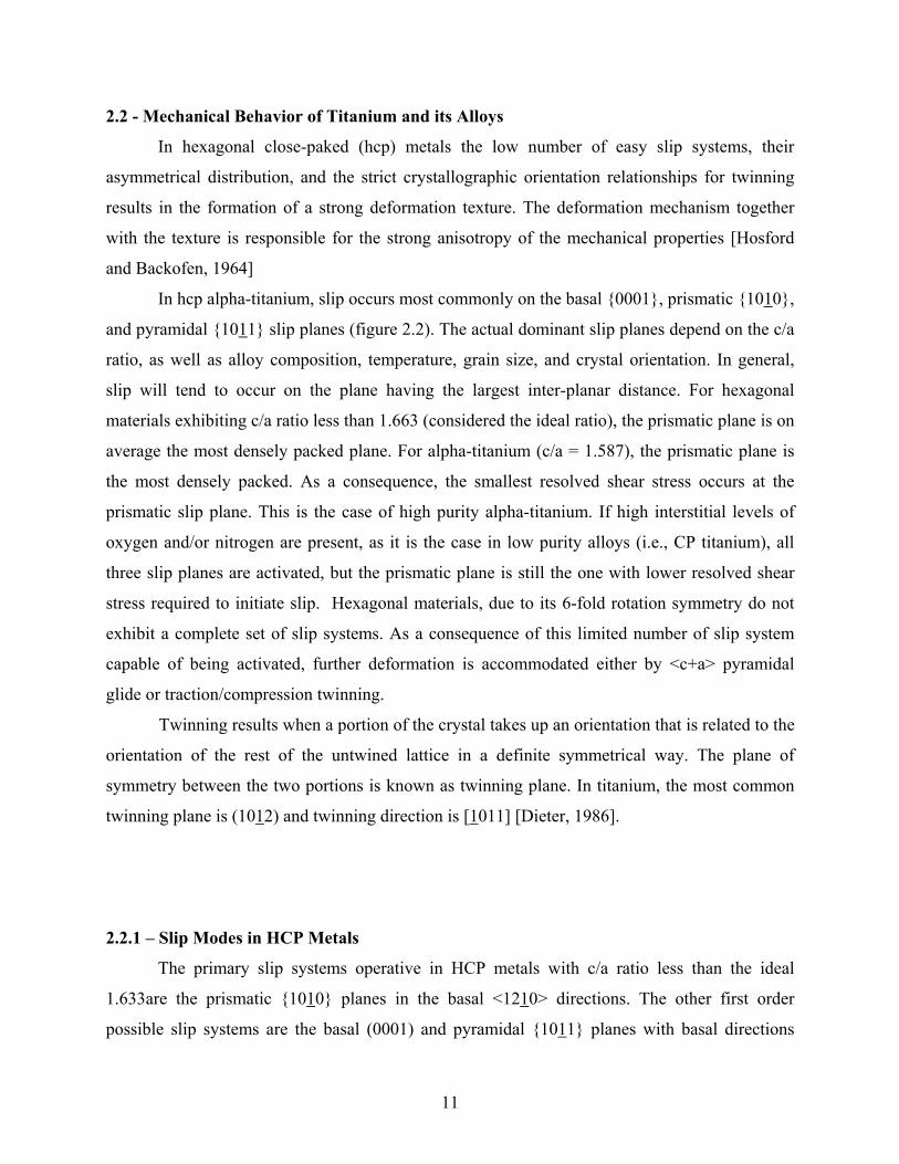
2.2 - Mechanical Behavior of Titanium and its Alloys
In hexagonal close-paked (hcp) metals the low number of easy slip systems, their
asymmetrical distribution, and the strict crystallographic orientation relationships for twinning
results in the formation of a strong deformation texture. The deformation mechanism together
with the texture is responsible for the strong anisotropy of the mechanical properties [Hosford
and Backofen, 1964]
In hcp alpha-titanium, slip occurs most commonly on the basal 0001, prismatic 1010,
and pyramidal 1011 slip planes (figure 2.2). The actual dominant slip planes depend on the c/a
ratio, as well as alloy composition, temperature, grain size, and crystal orientation. In general,
slip will tend to occur on the plane having the largest inter-planar distance. For hexagonal
materials exhibiting c/a ratio less than 1.663 (considered the ideal ratio), the prismatic plane is on
average the most densely packed plane. For alpha-titanium (c/a = 1.587), the prismatic plane is
the most densely packed. As a consequence, the smallest resolved shear stress occurs at the
prismatic slip plane. This is the case of high purity alpha-titanium. If high interstitial levels of
oxygen and/or nitrogen are present, as it is the case in low purity alloys (i.e., CP titanium), all
three slip planes are activated, but the prismatic plane is still the one with lower resolved shear
stress required to initiate slip. Hexagonal materials, due to its 6-fold rotation symmetry do not
exhibit a complete set of slip systems. As a consequence of this limited number of slip system
capable of being activated, further deformation is accommodated either by <c+a> pyramidal
glide or traction/compression twinning.
Twinning results when a portion of the crystal takes up an orientation that is related to the
orientation of the rest of the untwined lattice in a definite symmetrical way. The plane of
symmetry between the two portions is known as twinning plane. In titanium, the most common
twinning plane is (1012) and twinning direction is [1011] [Dieter, 1986].
2.2.1 – Slip Modes in HCP Metals
The primary slip systems operative in HCP metals with c/a ratio less than the ideal
1.633are the prismatic 1010 planes in the basal <1210> directions. The other first order
possible slip systems are the basal (0001) and pyramidal 1011 planes with basal directions
11

<1210>. These systems will provide combinations of 4 independent slip systems, since they all
occurs on the basal direction.
Figure 2.2 – The hexagonal unit cell (a) and the first order slip and twinning planes for hcp metals (b) [Dieter, 1986].
Differently from materials with cubic crystalline structure that posses 5 or more glide
systems, in hexagonal close packed metals the most common basal and prismatic glide modes
have only 2 or 3 independent glide systems respectively [Groves, 1963]. As a consequence, since
at least four or five independent slip systems are necessary to accommodate arbitrary plastic
strains, secondary systems like pyramidal glide with <c+a> Burger’s vector, or twinning systems
can be activated contributing to accommodate the imposed strain [Yoo, 1981 and Partridge,
1967]. Figure 2.3 shows the primary and secondary glide systems for Titanium.
Regarding hexagonal metals, the activation of slip and twinning systems is normally
affected by parameters like c/a ratio, interstitial constituent (i.e. Oxygen content principally in
the case of CP Ti), strain hardening, strain rate and temperature.
At room temperature, as a consequence of cold rolling, Ti deforms by prismatic glide
1010<1210>, pyramidal glide 1011<1120> with <a> Burger’s vector and secondary
1011<1123> with <c+a> Burger’s vector, 1012<1011> (and in some cases 1121 twinning
12

in tension and 1122<1123> twinning in compression [Rosi et al. 1956; Conrad, 1981; Chin,
1975].
Figure 2.3 – Glide systems in alpha titanium.
13

In the case of high purity titanium deformed in uniaxial compression at 20°C, it was reported
(via EBSD analysis), the activation of three types of twins: 1122<1123>, 1012<1011> and
1121<1126>, in the proportions of 40%-30%-30% respectively [Salem 2002, Kalidindi et al.
2004].
Zaefferer investigated the relation between the formation of cold rolling textures and the
activated glide and twinning systems during deformation of polycrystalline Titanium [Zaefferer,
2003]. Samples of three different titanium alloys (Ti-6Al-4V and two commercially pure
Titanium grades designated in the work as T40 (1000ppm O) and T60 (2000ppm O)) were
deformed up to 5% by uniaxial or biaxial. Zaefferer observed a considerable activity of <c+a>
and twinning in the case of the T40 alloy with a pronounced TD-type texture and for the T60
Alloy, the higher oxygen content completely suppressed twinning and strongly reduced <c+a>
activity resulting in a less developed TD-type texture which was a result of a combination of
<c+a> and basal slip. The results reported by Zaefferer are summarized below in the tables 2.3
and 2.4 and the main textures observed are presented in the figure 2.4.
Table 2.3- Number of grains showing a specific glide system for different samples Slip system TA3Z0 (%) TA3Z45 (%) TA3Z90 (%) TA1Z (%) TA1B (%) T401B (%) T601B (%)
<a>-Basal 1 (6) 3 (28) 4 (16) 2 (5) 11 (35) 5 (14) 9 (37)
<a>-Prismatic 4 (27) -- 1 (4) 9 (23) 3 (10) 2 (6) 1 (4)
<a>-Pyramidal 3 (20) 2 (18) 3 (12) 3 (7) 3 (10) 8 (21) 3 (13)
<a>-Screw 3 (20) 4 (36) 5 (20) 26 (65) 9 (30) 6 (16) 4 (16)
<c+a>-Pyramidal 4 (27) 2 (18) 12 (48) -- 5 (15) 13 (34) 5 (21)
Others T401B - <c+a>-Prismatic 4 (9) and T601B- <c+a>-Prismatic 2 (8)
Phillipe and Fundenberger [Phillipe et all, 1995, Fundenberger et all, 1997], working with
cp-Titanium grade 1(T35) and grade 2(T60) respectively, studied the activation of glide and twin
systems during cold rolling and observed the occurrence of 1010 <1120> prismatic slip and a
very low activity of Basal and pyramidal <a> slip. They also observed activation of two twinning
14

systems: 1012 tension twins and 1122 compression twins. In the case of second order
pyramidal slip <c+a> it was observed a low activity of this type of gliding up to 50% of
deformation but from this point up to 80% reduction in thickness, twinning is suppressed and to
accommodate further deformation in <c> direction, the <c+a> pyramidal gliding was activated
instead of 1122 compression twinning.
Table 2.4 - The most important deformation systems in hcp metals and their influence on the texture evolution [Zaefferer, 2003]. Burgers vector or
shear direction
Glide or
shear plane*
Name
Related cold-rolling
texture type
1/3<1120> (<a>) 0001
1010
1011
Basal glide
Prismatic glide
<a> Pyramidal glide
r-type [Sakai and
fine,1974],c-type
[Conrad, 1981]
r-type [Philippe et al.
1988]
1/3<1123> (<c+a>) 1011
1122
<c+a> Pyramidal (I) glide
<c+a> Pyramidal (II) glide
t-type
t-type
<1011> 1012 1012 Twin Under tension – c-type
(Ti); compression – r-
type (Zn)
<1126> 1121 1121 Twin Under tension – c-type
<1123> 1122 1122 Twin Under compression –
t-type
* Glide plane in case of dislocations, shear plane in case of twinning.
15

Figure 2.4 - Schematics of all investigations carried out and definition of sample short names. The starting texture of the different materials is given in the form of (0001) and /1010/ X-ray pole figures. Sample short names are composed as follows: (1) chemical composition; (2) sheet thickness in mm; (3) deformation mode; (4) angle between RD and tension direction (0°, 45°, 90°) or deformation degree (2%, 4%) [Zaefferer, 2003].
In titanium, Rosi et al. observed no twins of any type at 800°C, while McHarque and
Hamond reported a small amount of 1122 and 1121 twinning at 815°C. At room
temperature and below that titanium slips along the <1120> direction on the 1010, (0001) and
1011 planes. Changes in length along the c axis are not possible with <1120> slip alone,
requiring a slip direction lying out of the basal plane (0001). Such slip has been reported in
16

commercially pure titanium as a result from the motion of the <c+a> dislocations along the
<1123>. A length change along the c axis can also be accomplished by twinning. In titanium,
1012, 1121 and 1123 twins allow an extension along the c axis, while 1122, 1124
and 1010 twins allow a reduction in the c axis; whish generally becomes less important as the
deformation temperature increases. Paton and Backofen [Paton and Backofen, 1970]
investigating iodide titanium single crystals under compression at temperatures from 25°C to
800°C, have found that reduction of up to a few percent strain along the c axis is accommodated
almost entirely by 1122 twinning from 25°C to 300°C. According to their results, although
<c+a> slip is not responsible for a significant amount of strain below 300°C, it is important as a
means of accommodating the shear ahead of a propagating 1122 twin.
2.3 - Texture
The most commonly and important used materials for industrial practice, such as metals,
ceramics and some polymers are polycrystalline materials and their component units are referred
to as crystals or grains. Grain orientations in polycrystals are rarely random due to the processing
history that the polycrystalline materials are normally submitted to, such as solidification from
melting, hot rolling, cold rolling and annealing among other thermo-mechanical processes.
Therefore, in most materials there is a pattern in the orientations, which are present and a
tendency for the occurrence of certain orientations. This tendency is known as preferred
orientation of crystals or texture. The relevance of texture to materials lies in the fact that many
materials properties are texture-dependent. According to Bunge-1987, the influence of texture on
material’s properties is, in many cases, 20-50% of the properties values. Some examples of
properties which depend on the average texture of a material are: Young’s Modulus, Poisson’s
ratio, strength, ductility, toughness, magnetic permeability, electrical conductivity and thermal
expansion (in non-cubic materials) [Randle and Engler, 2000].
Texture, in hexagonal materials, is represented by the Miller indices hkil<uvtw> where
hkil corresponds to the family of crystallographic planes parallel to the surface of the sample
and <uvtw> corresponds to the family of crystallographic directions parallel to the rolling
17

direction (RD) of the sample. The resulting rolling textures, in the form of pole figures, as a
function of c/a ratio is shown in figure 2.5.
Figure 2.5 – Sheet textures in hcp materials as a function of c/a ratios (schematically).
18

The ideal cold rolling texture component is represented in figure 2.6 and other typical
textures in hexagonal materials are shown in figure 2.7.
Figure 2.6 – Ideal cold rolling texture component for flat-cold rolled titanium: 2115 <1010>.
Texture can be determined by means of X-ray diffraction, neutron diffraction and
electron diffraction using Transmission Electron Microscope (TEM) or Scanning Electron
Microscope (SEM). X-ray diffraction is the most commonly applied technique but the neutron
and electron diffraction techniques are gaining interest because it permits one to correlate
microstructures, neighbor relations and texture [Kocks, 1998].
Among the ways to describe texture, pole figure (PF), inverse pole figure (IPF) and
orientation distribution function (ODF) are the most usual methods. Pole figure is a projection
[Cullity; 2001], more often represented as a stereographic projection, which shows the variation
of pole density with pole orientation for a selected set of crystal planes having the rolling
direction (RD), the transversal direction (TD) and the normal direction of the sample as reference
axis.
19

Figure 2.7 – Typical textures [Wang, 2003].
20

Pole figures are measured using x-ray diffraction and in order to have a specific (hkil)
reflection, the following condition, known as Bragg’s law (equation (2.1)), must be satisfied.
nλ = 2 dhkl . sin θ (2.1)
During the pole figure measurement, to determine a pole density, the x-ray detector
remains stationary at the proper 2θ angle, to receive the (hkil) reflections, while the specimen
rotates in two particular ways. These rotations permit a complete scanning of the specimen’s
surface and the positioning of the sample on the texture goniometer is shown in figure 2.8.
Figure 2.8 - Positioning and movement of the sample on the texture goniometer inside the X-ray machine (a). The relation between crystallite coordinates (Xc, Yc, Zc) and sample coordinates (Xs, Ys, Zs), (b), (c) and (d).
21

The α and β angles, which are respectively the polar and the azimuthal angles, define the
movements of the sample during the pole figure measurement.
The inverse pole figure (IPF) is a pole density projection of the (hkil) planes referred to
the stereographic triangle. Inverse pole figure presents an advantage over the pole figure because
an IPF shows the density distribution of all planes within the stereographic triangle instead of
showing only the density of a specific crystallographic plane (see figure 2.9).
RD
(0002) (1010) (2110)
TD
a)
ND TD RD (1010)
(0002) (2110)
b)
Figure 2.9 – As received material: a) Pole figures and b) Inverse pole figures.
The pole figure and the inverse pole figure are very helpful tools however principal
orientations of the texture cannot be precisely determined from them because they do not provide
information regarding the crystallographic directions in the plane of the sample. The figure 2.10
22

exemplifies a situation where two different texture components, the cold rolling and the
recrystalization components, exhibit the same (0002) pole figure, which can be misleading if the
analysis is based only on basal pole figures.
Figure 2.10 – Pole figure representation of the cold rolling and the recrystalization texture components.
It has been well established that the orientation distribution in textured materials can be
qualitatively as well as quantitatively evaluated by the crystallite orientation distribution function
analysis (ODF) developed by Bunge and by Roe [Bunge, 1982; Roe, 1965]. The ODF describes
the frequency of occurrence of particular orientations in a three-dimensional orientation space.
This space is defined by three Euler angles (ψ, θ, φ) which are related to the macroscopic axis of
the sample, defined as rolling direction (RD) axis, transversal direction (TD) axis and normal
direction (ND) axis through a set of three consecutive rotations that must be given to each
crystallite in order to bring its crystallographic axes into coincidence with the specimen axes.
23

Figure 2.11 shows the rotations where ψ represents a rotation around the ND axis, θ represents a
rotation around the TD axis and φ represents a second rotation around the ND axis.
Figure 2.11 - Three consecutives Euler rotations defining an orientation.
ODF is a three dimensional description of texture but direct measurement of ODF is not
possible since conventional texture goniometry is only capable of determining the distribution of
crystal poles of diffracting planes normal, i.e., pole figures. Mathematical models have been
developed which allow the ODF to be calculated from the numerical data obtained from several
pole figures. Therefore, in order to compute the orientation distribution function for a
polycrystalline sample, pole figures measurements are required. The number of pole figures
needed for ODF calculation depends upon the crystal symmetry of the sample that is being
measured. For HCP materials, as it is the case of titanium, a minimum of five pole figures are
needed. The most widely adopted methods for calculating ODFs are those proposed
independently by Roe (1965) and by Bunge (1982), who used generalized spherical harmonic
functions to represent the crystallite distributions. The three Euler angles employed by Bunge to
describe the crystal rotations are φ1, Φ and φ2, whereas the set of angles proposed by Roe are
referred to as ψ, θ and φ respectively. The relationships between the Bunge and the Roe angles
are the following:
φ1 = π/2 - ψ; Φ = θ; φ2 = π/2 - φ
24

According to Roe, 1965, an ODF may be expressed as a series of generalized spherical
harmonics in the form of equation (2.2):
∞ l l
(ψ, θ, φ) = Σ Σ Σ Wlm Zlmn (cos θ). exp (-imψ). exp(inφ) (2.2)
l=0 m=-1 n=-1
Where Wlmn are the series coefficients and Zlmn (cosθ) is a generalization of the associated
Legendre functions, the so-called augmented Jacobian polynomials.
For hexagonal/orthotropic crystal/specimen symmetry, a three-dimensional orientation
volume may be defined by using three orthogonal axes for ψ, θ and φ with each of the Euler
angles ranging from 0 to 90°. The value of the orientation density at each point in this volume is
simply the intensity of that orientation in multiples of random units. Regions of higher and lower
orientation density are separated by three-dimensional contour surfaces and it is usual to take a
series of parallel sections through this space for ready visualization of the data contained in the
three-dimensional plot. In the case of hcp materials, due to their crystal symmetry, the
fundamental space can be reduced to the space spanned by the Euler angles ψ (from 0 to 90°),
θ(from 0 to 90°) and φ(from 0 to 60°) with sections every 5 or 10 degrees. Davies [Davies et al.,
1971] published a set of charts for hexagonal materials designed to aid on the task of indexing
the texture components of rolled materials with hexagonal symmetry. In this development
Davies has used a definition of Euler angles by Roe and has taken crystal directions <0002>
parallel to ND and <1010> parallel to RD (see figure 2.12).
Figure 2.12 – Relationship between sample and crystal axis directions.
25

The charts published by Davies are shown in the figure 2.13 and in figure 2.14 an
example of the advantage of using the ODF in texture analysis.
Figure 2.13 – Constant φ sections through the Eulerian space: a)0°, b)20°, c)30°, d)40 and e)60°
26

Figure 2.14 – Location of the cold rolling and recrystalization components on the constant phi sections of the Euler space using Roe’s definition [Roe, 1965]. 2.3.1- Cold Rolling Texture
Hexagonal materials, such as, titanium and zirconium, have a limited number of slip
systems and generally develop a strong texture after cold rolling. Knight, 1978; investigated the
texture evolution of commercially pure titanium sheets after cold rolling at 21.4% and 89.4% of
reduction and observed that the most intense texture component, for both degrees of reduction
was the (2115) [0110]. Guillaume et al., 1981, when working with cold rolled titanium sheets,
found the same result. The (2115) [0110] orientation is 35° around the (0002) pole in the
transversal plane, which involves a rotation of the (0002) pole around the rolling direction, in the
plane defined by the transversal and the normal directions. Philippe et al. [Philippe, 1984], have
also found the same texture components after cold rolling of titanium and zirconium alloys.
27

Inagaki [Inagaki, 1991] working with hot rolled and annealed pure titanium presenting a very
strong texture, found that after cold rolling reductions below 30% the textures were weakened by
twinning and slip rotations. At cold rolling reductions between 30 and 50% twinning occurred
less frequently and at rolling reductions above 50%, crystal rotation about <0110>//RD axis is
induced by slip deformation. Orientations located near the 0001 <0110> were rotated toward
the 2115 <0110> orientation, becoming stable at this orientation at rolling reductions above
80%. Inagaki also found that the [0001]//ND fiber texture increased remarkably at rolling
reduction between 30 and 50% and that it decreased rapidly at rolling reductions above 50%. The
[0110]//RD fiber, on the other hand, developed at rolling reductions above 50%.
2.3.2- Hot and Warm Rolling Texture
In the past, hot rolling textures in titanium have been studied by only few investigators
and warm rolling textures in titanium have called even less attention from the researchers.
Inagaki [Inagaki, 1990] investigated the effect of hot rolling temperature (750, 800, 850, 900 and
950°C) on the development of hot rolling textures on commercially pure titanium plates.
According to Inagaki, the textures observed in the specimens hot rolled at temperatures below
800°C are essentially the same as the cold rolling texture and their main orientation is 2115
<0110>. Hot rolling at temperatures between 800 and 850°C enhances the development of the
2110 <0110> and 2118 <8443> main orientations, which seem to be formed by the
recrystallization that occurs during and after hot rolling. Hot rolling at temperatures above 880°C
results in the formation of a strong transformation texture where the 2110 <0110> texture
component, derived from the BCC β phase rolling texture, is the main orientation.
2.4 – X-ray Peak Profile Analysis
In order to improve and to control the mechanical proprieties of any material it is
important to understand and to explain how variables such as dislocation density, dislocation
type and slip system activation affect the formation and evolution of certain microstructures
28

during the deformation process. The study and determination of the dislocations slip systems
type is usually carried out with conventional techniques such as TEM. However, when the
material is highly deformed and the dislocation density reaches values as high as 1010/cm2, TEM
analysis is rather difficult. Also, throughout the sample preparation process required for TEM
experiments the original microstructure may change. Other alternatives on investigating the
microstructure are X-ray and neutron diffraction techniques. In recent decades, new applications
for the X-ray diffraction method (traditionally used for phase identification, quantitative analysis
and the determination of structure imperfections), have extended its usage to new areas, such as
the determination of crystal structures and the extraction of microstructural properties of
materials. Recent works have shown that X-ray diffraction peak profile analysis (XDPPA) is a
powerful alternative to transmission electron microscopy for describing the microstructure of
crystalline materials and providing information about the dislocation densities and dislocation
type extracted from the X-ray pattern [Ungár, 1999; Ribárik, 2001; Dragomir, 2002; Scardi,
2002; Glavicic, 2004; Scardi 2004; Ungár, 2004; Dragomir, 2005a and 2005b]. Besides that,
since the parameters provided by the two different methods are never identical, XDPPA is also
complementary to TEM enabling a more detailed understanding of microstructures.
X-ray diffraction peaks broaden when the crystal lattice becomes imperfect. The
microstructure means the extent and the quality of lattice imperfectness. According to the theory
of kinematical scattering, X-ray diffraction peaks broaden either due to crystallites smallness
(≈1μ ), lattice defects are present in large enough abundance ( in terms of dislocations this means
a dislocation density larger than about 5x10¹²m-2), stress gradients and/or chemical
heterogeneities.
Peak broadening is caused by crystallite smallness, lattice defects, stress gradients and/or
chemical heterogeneities. As a consequence of these deviations from perfect crystalline lattice
the shape of the X-ray diffraction lines no longer consists of narrow, symmetrical, delta-function
like peaks, such as the diffraction lines given by an ideal powder diffraction pattern. The
aberrations from the ideal powder pattern can be conceived as: (i) peak shift, (ii) peak
broadening, (iii) peak asymmetries, (iv) anisotropic peak broadening and (v) peak shape. The
main correlation between these peak aberrations and the different elements of microstructure are
summarized in table 2.5.
29

Table 2.5 – The most typical correlations between diffraction peak aberrations and the different elements of microstructure (Ungár, 2004). Sources of strain Peak aberrations
shift broadening asymmetry Anisotropic
broadening
shape
Dislocations √ √ √ √
Stacking faults √ √ √ √ √
Twinning √ √ √ √ √
Microstresses √
Long-range internal stresses √ √
Grain boundaries √ √
Sub-boundaries √ √
Internal stresses √
Coherency strains √ √ √
Chemical heterogeneities √ √ √
Point defects √
Precipitates and inclusions √ √
Crystallite smallness √ √ √
The effect of these defects can be divided into two main types of broadening: size- and
strain broadening. The first depends on the size of coherent domains and may include effects of
stacking and twin faults and sub-grain structures (small-angle grain boundaries) whereas the
latter is caused by different lattice imperfection, especially dislocations. The two different effects
interplay with each other and very often are not easy to separate. Krivoglaz [Krivoglaz, 1969]
has shown that strain broadening can be described, in general, in terms of broadening caused by
dislocations. In the case of single crystals or coarse-grained polycrystalline materials, strain
broadening caused by dislocations can be well described by a special logarithmic series
expansion of the Fourier coefficients [Krivoglaz, 1969; Wilkens, 1970; Groma et al., 1988,
Ungár et al., 1989]. When grain size plays a role, the two effects (i.e. size and strain broadening)
overlap. In such cases the grain size or the properties of the dislocation structure can only be
30

determined by the correct separation of the two effects. Two classical procedures are employed
in order to separate the strain and domain-size components of the broadening: Williamson-Hall
method and Warren-Averbach method. The first procedure [Williamson and Hall, 1953] is based
on the full width at half maximum (FWHM) and the integral breadths while the second is based
on the Fourier coefficients of the profiles [Warren and Averbach, 1950; Warren, 1959]. The
particle-size and dislocation microstrains are convoluted but can be separated, because the
particle-size broadening is independent of the order of the diffraction line, whereas the strain
broadening is not. In the Warren-Averbach method, the diffraction line profile is transformed
into its Fourier components and processed in order to separate the two broadening effects (after
correction for instrumental broadening). Evaluations carried out with both methods provide
apparent size parameters of crystallites or coherently diffracting domains and values of the mean
square strain but grain shape anisotropy and also strain anisotropy can turn difficult and
complicate the evaluation process [Louër et al., 1983; Caglioti et al., 1958]. In practical terms,
strain anisotropy means that neither the full width of half maximum (FWHM) in the Williamson-
Hall plot [Williamson and Hall, 1953] nor the Fourier coefficients in the Warren-Averbach
analysis [Warren and Averbach, 1952; Warren, 1959] are smooth functions of the diffraction
vector g. Ungár proposed that a way to interpret strain anisotropy is to assume that dislocations
are one of the major sources for lattice distortions [Ungár and Borbély, 1996]. Two different
approaches can well account for the phenomenon, especially in the case of random
polycrystalline or powder specimen. One is a phenomenological approach assuming that the
random displacements of atoms are weighted by the anisotropic elastic constants of the crystal
[Stephens, 1999] and the FWHM is scaled by the fourth order invariants of the hkl indices, given
for different crystal classes e.g. by Nye, (1957) or Popa, (1998). The other approach operates
with the anisotropic diffraction contrasts of dislocations [Stokes and Wilson, 1944; Ungár and
Borbély, 1996]. In the case of randomly oriented polycrystalline or powder specimen the
dislocation model has been shown to be formally equivalent to the phenomenological approach
[Ungár and Tichy, 1999] and the model is able to provide quantitative results, which have
physical relevance to the microstructure of the crystal [Cheary et al., 2000]. An advantage of this
model is that it also works in the case of a heavily deformed polycrystalline material or a single
crystal [Mohamed et al., 1997; Cheary et al., 2000; Borbély et al., 2000], situations in which a
strong preferred orientation is present.
31
In polycrystalline material populated with dislocations the anisotropic line broadening
can be taken into account by using that the dislocation model of the mean square strain, <εg,L2>,
(where L is the Fourier length and εg is the distortion tensor component in the direction of the
diffraction vector, g) [Wilkens, 1970a and 1970b]. In this model the dislocations are assumed to
have a restrictedly random distribution within a region defined by Re as the effective outer cut-
off radius [Wilkens, 1970a]. Here the anisotropic effect can be summarized in the average
contrast factors, C, which depends on the relative orientations of the line and Burgers vectors of
dislocations and the diffraction vector [Ungár and Borbély, 1996; Wilkens, 1970b; Klimanek and
Kuzel, 1988; Kuzel and Klimanek, 1988 and 1989; Ungár and Tichy, 1999; Dragomir and
Ungár, 2002]. The contrast factor of dislocations is a measure of the “visibility” of dislocations
in the X-ray diffraction experiments. Since, the contrast effect is mainly a characteristic of
dislocations, the theoretical values of the contrast factors and those obtained from the profile
evaluation enable the determination of the active dislocation slip system(s) in the studied sample
[Klimanek and Kuzel, 1988; Kuzel and Klimanek, 1988 and 1989; Ungár and Tichy, 1999;
Dragomir and Ungár, 2002].
Because of the complexity of the mechanical properties of hexagonal crystals [Chung &
Buessem, 1968; Gubicza et al., 2000; Solas et al., 2001; Tomé et al., 2001] for a better
understanding of the bulk dislocation structure and the Burgers vector populations it is desirable
to complement TEM studies by X-ray diffraction profile analysis. When comparing the
hexagonal crystal to the cubic crystal it becomes evident the higher level of complexity involved
when dealing with the hexagonal systems. Instead of three elastic constants hexagonal crystals
exhibit six elastic constants and two lattice constants (c and a) while cubic systems have only one
(a). Moreover instead of one, hexagonal crystal present two different types of anisotropy: shear
and compression [Chung and Buessem, 1968]; and finally, while in cubic systems there is one
major slip system, in hexagonal there are three different major slip systems related to the three
glide planes: basal, prismatic and pyramidal. If it is taken in account the different glide directions
and dislocation character (i. e., edge and screw) it is possible to group the slip systems into
eleven sub-slip-systems as shown in Table 2.6 [Yadav and Ramesh, 1977; Jones and Hutchinson,
1981; Honeycombe, 1984; Castelnau et al., 2001]. Dragomir and Ungár (2002) have recently
published a modified methodology to obtain the contrast factors for both cubic and hexagonal
crystals. They concluded that, at the actual state of the art regarding line broadening analysis, it
32

is impracticable to compile the dislocation contrast factors for hexagonal systems in a similar
manner as it was done for cubic crystals and instead, they proposed to compile the average
contrast factors of the sub-slip-systems. The average contrast factor of a specific sub-slip-system
in a hexagonal crystal can be given by three parameters versus the fourth-order invariant of the
hkil Miller indices [Ungár and Tichy, 1999]: C hk.0, q1 and q2 and once these parameters are
determined all average contrast factor corresponding to the sub-slip-system in question can be
obtained [Dragomir and Ungár, 2002].
Table 2.6 - The most common slip systems in hexagonal crystals: (a) Edge dislocations and (b) Screw dislocations. (a) Edge dislocations:
Major slip systems
Slip-systems Burgers vector Slip plane Burgers vector types
Basal
BE >< 0112 0001 a
PrE >< 1102 0101 a
PrE2 >< 0001 0101 c
Prismatic
PrE3 >< 1132 0101 c + a
PyE >< 0121 1110 a
Py2E >< 1132 2112 c + a
PyE3 >< 1132 1211 c + a
Pyramidal
PyE4 >< 1132 1110 c + a
(b) Screw dislocations:
Slip-systems
Burgers vector Burgers vector types
S1
>< 0112 a
S2
>< 1132 c + a
S3
>< 0001 c
33

2.4.1 - X-ray Peak Profile Analysis from MWP and Methodology for Determining the
Burgers Vector Populations
It is well known that the Fourier coefficients of the physical profiles can be written as a
multiplication of the Fourier coefficients corresponding to the size and distortion effect [Ungár
and Tichy, 1999]:
AL = ALS AL
D = ALS exp [- 2π2L2g2 <εg,L
2> ] (2.3)
where S and D indicate size and distortion, g is the absolute value of the diffraction vector,
<εg,L2> is the mean square strain and L is the Fourier variable. As shown in [Wilkens, 1970a and
1970b; Krivoglaz, 1996] in a dislocated crystal the mean square strain can be written in terms of
dislocation density and the strain anisotropy, which can be taken in account by introducing the
dislocation contrast factors, <εg,L2> ≅ (ρ 2Cb /4π) f( ), where and b are the density and the
modulus of the Burgers vectors of dislocations and 2Cb is the average contrast factor of the
dislocations present in the sample multiplied by the square of the dislocations burgers vector.
f( )-function is the Wilkens’s function, where =L/Re, Re is the effective outer cut-off radius of
dislocations, L is the Fourier length defined as nλ/2(sinθ2-sinθ1) with n being an integer starting
from zero, λ the x-ray wave length and (θ2-θ1) the angular range of the measured profile
[Wilkens, 1970a].
Contrast effect of dislocations depends not only on the material, but also on the relative
orientation of the diffraction vector, g, line vector, l, and Burgers vector, b [Klimanek and Kuzel,
1988; Kuzel and Klimanek, 1988 and 1989; Dragomir and Ungár, 2002]. Due to this in the case
of hexagonal crystals the three major slip systems (basal, prismatic and pyramidal) have to be
divided in 11 sub-slip systems by taking into account the different slip system types and the
dislocation character (i.e. edge or screw). These eleven sub-slip-systems are illustrated in figure
2.16 and listed in table 2.6. It has been shown in earlier studies that in the case of hexagonal
crystals for a given sub-slip system the average contrast factor of dislocation can be written as
[Dragomir and Ungár, 2002]:
34

C hk.l = C hk.0 [1 + q1x + q2 x2 ] (2.4)
where x = (2/3)(l/ga)2, q1 and q2 are parameters which depend on the elastic properties of the
material, C hk.0 is the average contrast factor corresponding to the hk.0 type reflections, a is the
lattice constant in the basal plane, g is the diffraction vector and l is the last index of the hk.l
reflection for which the C hk.l is evaluated. The equation (2.4) is valid only when it can be
assumed that within a sub-slip system the dislocation can slip with the same probability in all
directions permitted by the hexagonal crystal symmetry. This equation also means that the
average contrast factors corresponding to a specific sub-slip-system and material constants
(elastic constants C11/C12, C13/C12, C33/C12, C44/C12 and the lattice constant c/a) have to follow a
parabola as a function of x having the parameters C hk.0, q1 and q2 as parameterization
parameters. In the case of Titanium, the parabolas corresponding to the eleven sub-systems
described in table 2.6 and shown in figure 2.16 are presented in the figure 2.15.
Figure 2.15 – The parabolas describing the average contrast factors for the eleven slip systems, in the case of Titanium, as a function of x = (2/3)(l/ga)2 [Dragomir et al., 2002].
35

BASAL
<2 1 1 0> 0001
PRISMATIC
< 2 110>01 1 0 < 2 113>01 1 0 <0001>1 1 00
PYRAMIDAL
< 1 2 1 0 >10 1 1 < 2 113 >10 1 1 < 2 113 >11 2 1 < 2 113 >2 1 1 2
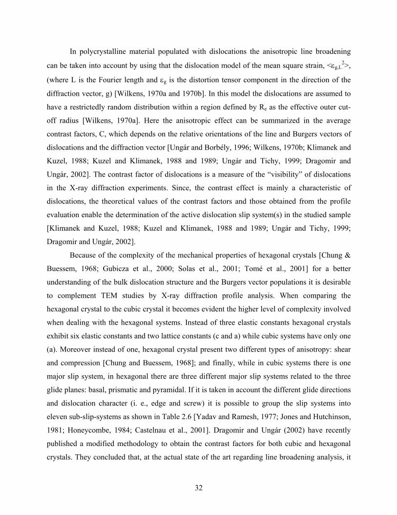
Figure 2.16 - Slip systems in hexagonal crystal systems [Honeycombe, 1984; Klimanek and Kuzel,1988]. As it has been shown by Dragomir and Ungár, in the case of hexagonal crystal the measured
average )(
2m
Cb characteristic to the examined sample can be written as follows [Dragomir and
Ungár, 2002]:
)(2
m
Cb =∑=
N
i
i
i
i bCf1
2)( (2.5)
36
where N is the number of the different activated sub-slip systems, )(i
C is the theoretical value of
the average contrast factor corresponding to the ith sub-slip system and fi are the fractions of the
particular sub-slip systems by which they contribute to the broadening of a specific reflection.
On the left hand side of the equation (2.5) the m superscript refers to the measurable strain
anisotropy parameter, 2Cb . For the hexagonal crystal structure, equation (2.5) can be written for
the three fundamental Burgers vectors types defined in the hexagonal systems: b1=1/3<2110>,
b2=<0001>, and b3=1/3<2113>:
)(
.2
m
lhkCb = 21b ∑
><
=
aN
i
i
i Cf1
)( + 22b ∑
><
=
cN
j
j
j Cf1
)( + 23b ∑
>+<
=
acN
n
n
n Cf1
)( (2.6)
where N<a>, N<c> and N<c+a> are the numbers of sub-slip systems with the Burgers vector
types <a>, <c> or <c+a>, respectively. The possibility of measuring q1 and q2 offers three
independent equations and eleven unknowns. It means that equation (2.6) can give an exact
solution only by making certain assumptions about the activated dislocation slip systems. In the
present work it is assumed that a particular Burgers vector type has random (or uniform)
distribution in the different slip systems. In this case equation (2.6) can be written:
)(
.2
m
lhkCb =∑=
3
1
2)(
i
i
i
i bCh (2.7)
where hi is the fraction of the dislocations population in the sample with the same Burgers
vector, bi. )(iC is the averaged contrast factor over the sub-slip systems, for the same Burgers
vector type. Inserting equations (2.4) into (2.7) the following three equations are obtained:
)(1
mq = ∑=
3
1
)(1
2)(0.
1
i
i
i
i
hki qbChP
, , (2.8)
37
)(2mq = ∑
=
3
1
)(2
2)(0.
1
i
i
i
i
hki qbChP
(2.9)
∑=
3
1i
ih =1 (2.10)
where P=∑=
3
1
2)(0.
i
i
i
hki bCh =)(
0.2
m
hkCb and 0≤ hi ≤1. To solve equations (2.8), (2.9) and (2.10) the
numerically calculated values of C hk.0, q1 and q2 for all sub-slip systems are required. The
theoretical values of C hk.0, q1 and q2 for the most common sub-slip systems were published
previously elsewhere [Dragomir and Ungár, 2002]. The contrast factor of dislocation for
hexagonal crystals in elastic anisotropic and isotropic media have been treated by Kuzel and
Klimanek [Klimanek and Kuzel, 1988; Kuzel and Klimanek, 1988 and 1989].
The measured values of q1 and q2 parameters are obtained from the Multiple Whole
Profile (MWP) fitting procedure [Ribárik et al., 2001]. In this procedure the Fourier-transformed
of multiple hkl reflections are fitted simultaneously by equation (2.3). Here, throughout the q1
and q2 parameters in equation (2.4), the dislocation contrast factor becomes a fitting parameter.
Finally, the q1(m) and q2(m) parameters obtained for the sub-slip-systems families are used in the
analysis of Burgers vector populations [Dragomir and Ungár, 2002] providing a prediction of
slip systems activity during the deformation process.
2.5 – Self-Consistent Modeling of Deformation Texture
The modeling of deformation texture evolution based on the formulation of the plasticity
of polycrystalline materials has received considerable attention and has been the object of many
studies and different approaches [Voigt, 1889; Reuss, 1929; Morris, 1970; Kroner, 1972;
Hutchinson, 1976; Ahzi, 1987; Canova et al., 1989].
As early as 1938, Taylor proposed a uniform strain model, which assumes that the
imposed plastic strain in each grain is identical to the macroscopic plastic strain [Taylor, 1938].
38
Models based upon Taylor’s assumption [Bishop and Hill 1951; Bunge 1970] have often
demonstrated first-order agreement with the measurement of mechanical anisotropy of
polycrystalline materials. However, the hypothesis of plastic strain uniformity is somewhat crude
and it has been shown to fail when plastic strain heterogeneities are evident, as it is the case of
uniaxial compression of fcc polycrystalline metals, uniaxial tension of bcc polycrystalline metals
and in general for polyphase materials.
For the case of small deformations, a self-consistent approach was proposed and
developed by different authors [Hill, 1965 and 1967; Hutchinson, 1970and 1976; Kröner, 1961;
Berveiller-Zaoui, 1980]. This approach takes into account the interaction of each grain with the
surrounding environment. Here, the medium (surrounding) is replaced by an equivalent medium
assumed to be a homogeneous equivalent medium (H.E.M). An extension to large elastoplastic
deformations was proposed by Iwakuma and Nemat-Nasser [Iwakuma and Nemat-Nasser, 1984]
and one application to large elastoviscoplastic deformations by Nemat-Nasser and Obata
[Nemat-Nasser and Obata, 1987]. An extension to large deformation plasticity has been
developed by Iwakuma and Nemat-Nasser [Iwakuma and Nemat-Nasser, 1984] and used for
two-dimensional problems. Hutchinson [Hutchinson, 1976] used an upper bound theorem and
self-consistent model proposed by Hill [Hill, 1965 and 1967] to derive macroscopic relations
between stress and strain-rates for a creep power law polycrystalline material in small
deformations.
The so-called Relaxed Constraints theory [Honneff and Mecking, 1978; Kocks and
Canova, 1981; Houtte, 1981] takes into account the strain heterogeneities produced by
anisotropic grain shapes and the predicted results have a better agreement with experiments. This
is true particularly in some specific cases, like large strain rolling and torsion of fcc metals.
Asaro and Needleman have proposed an extension of Taylor theory for large deformations
including elastic deformations [Asaro and Needleman, 1985]. It should be noticed that all
theories based on Taylor’s strain uniformity only fulfill compatibility conditions but not
equilibrium conditions at grain boundaries.
In 1987, using a scheme developed by Zeller and Dederichs (1973) in heterogeneous
elasticity, Molinari, Canova and Ahzi [Molinari et al., 1987] proposed a self-consistent approach
for the large deformation polycrystal viscoplasticity which they applied to the prediction of
deformation textures in the cases of tension, compression, rolling and torsion [Molinari et al.,
39
1987]. Almost at the same time, Nemat-Nasser and Obata [Nemat-Nasser and Obata, 1987] also
proposed a model to approach the macroscopic behavior of an elastic viscoplastic polycrystal by
using Hill’s self-consistent model [Hill, 1989]. They applied their theory to a plane problem with
double slip modelization of the single crystal behavior.
In this work it was used the approach proposed by Molinari, Canova and Ahzi [Molinari
et al., 1987], which consists of a self-consistent formulation for the large deformation polycrystal
viscoplasticity. The properties of the polycrystal are developed from the single crystal behavior
[Zeller and Dederichs, 1973; Berveiller and Zaoui, 1980]. In this approach, equilibrium and
incompressibility equations are used to arrive at an integral equation for local velocity gradient.
This integral equation can be solved via different approximate schemes. In the self-consistent
model of Molinari [Molinari et al., 1987], a grain is considered as an inclusion embedded in a
homogeneous equivalent medium. The interaction law derived from the integral equation results
in a nonlinear relation between stress and strain rate, which is solved by a straightforward
Newton method.
2.5.1 – The Single-Crystal Constitutive Law
As in certain models [Hutchinson, 1976; Pan and Rice, 1983; Asaro and Needleman,
1985] of single-crystal behavior, here it is assumed that slip is slightly sensitive to velocity. We
also assume that the plastic-shear rate on slip system s depends on the shear stress τsγ& s resolved
on the system, according to the following law:
( )msss
00 γγττ &&= (2.11)
The parameter m is the strain-rate sensitivity coefficient. τs
is associated with the deviatoric
Cauchy stress tensor by the relation
SmSm s
ij
s
ij
s :==τ (2.12)
where
40

s
j
s
i
s
ij nbm = (2.13)
n
s and b
s are the normal to the slip plane and the slip direction, respectively, for slip system s.
and represent a reference stress and the corresponding reference strain velocity,
correspondingly.
s
0τ s
0γ&
The strain-velocity tensor D is defined by
Dij = ( υi,j + υj,i)/2 (2.14)
where υi are the components of the displacement velocity. The comma designates the derivative
with respect to the reference coordinates associated with the laboratory. The strain-velocity
tensor is associated with the microscopic shear velocity by the relation:
∑=s
ss
ijij rD γ& (2.15)
where,
( ) 2/s
ji
s
ij
s
ij mmr += (2.16)
By using the microscopic stress-strain relation (2.11) and the definition of resolved shear stress
(equation (2.12)), the single-crystal constitutive law, where elasticity is neglected, finally results
in a non-linear relation between the strain velocity and the deviatoric Cauchy stresses Skl:
n
s
kl
s
kls
ij
ij Srr
D
⎟⎟⎠
⎞⎜⎜⎝
⎛=
00 τγ& (2.17)
where,
n=1/m (2.18)
The variation of as a function of time characterizing the microscopic intracrystalline
work hardening and the variation of are associated with the orientations changes of the crystal
s
0τ
s
ijr
41

lattice. The development of the microscopic work hardening is represented by the following
relation:
∑=r
rsrs H γτ &&0 (2.19)
where the terms Hsr represent the elements of the microscopic strain-hardening matrix.
The crystal-lattice rotation-velocity tensor Ω* is obtained from the difference between the
total rotation-velocity tensor ΩP and the plastic rotation velocity.
Ω = Ω* + ΩP (2.20)
where, Ω is the antisymmetric part of the displacement-velocity gradient L
Ω = ( L – LT )/2 (2.21)
and ΩP is given bu the following relation
( ) 2/s
S
STTSP mm γ&∑ −=Ω (2.22)
Knowing the total-rotation velocity Ω and the microscopic shear velocity , it can be
determined the crystal-lattice rotation velocity from equation (2.20).
sγ&
The nonlinear relation (2.17) may be written in the form of:
Dij = Gij (S) (2.23)
By inverting this relation, one can express the stresses S as a function of the strain-
velocity tensor D
Skl = Fkl (D) (2.24)
The solution of equation (2.24) is unique since a convex viscoplastic potential exists. The
tangent behavior is obtained by the Taylor development to first order from the law (2.24)
concerning the applied strain velocity D’:
42

( ) 0' klmnklmnkl SDDAS += (2.25)
with
( ) ( )1
''−
⎥⎦⎤
⎢⎣⎡
∂∂
=∂∂
=klmnmn
klklmn
S
GD
D
FDA (2.26)
where (∂G/∂S) is the Jacobian matrix of the function G(S).
( )'0 DSkl is defined by:
( ) ( ) klmnklmnkl SDDADS +−= ''0 (2.27)
The tensor A has the following symmetry properties:
Aklmn = Alkmn = Aklnm = Amnlk
The Cauchy stress tensor is obtained by addition of the hydrostatic term to the deviator
term S.
= A (D):D + S0 (D) – pI (2.28)
where p is the hydrostatic pressure and I the identity tensor of second order.
2.5.2 – Polycrystal Constitutive Law
Locally, the law defining the behavior of the medium (HEM) is given by the equation
(2.28), where both A and S0 depend on the position r. In each grain A and S0 depend on the
microscopic work hardening and grain orientation.
Imposing to the polycrystal a macroscopically-homogeneous displacement-velocity
gradient L
43

jiij VL ,= (2.29)
which satisfies the incompressibility condition iiL = 0, and a macroscopic pressure p , the aim is
to obtain the local pressure p and the displacement-velocity L defined by:
Lij = Vi,j (2.30)
The equilibrium equation must be satisfied throughout the polycrystal and in the absence of body
forces, this may be expressed by:
σij,j = 0 (2.31)
According to equation (28.2), the equilibrium equation is written:
( ) 0,0,,, =−+ ijijjlkijkl pSVA (2.32)
The macroscopic constitutive law is represented by the tangent behavior
000 SDAS += (2.33)
where D is the applied strain velocity, and A0 and S00 are dependent of D .
Decomposition of the tensors A (and S0) into the sum of a uniform part A0 (and S00 ) and
a part dependent of the spatial position r leads to
( ) ( )rr AAA~0 +=
( ) ( )0000 ~rr SSS +=
(2.34)
By using this decomposition in equation (2.32) it is obtained the following Navier’s
equations:
0,,
0 =+− ijljkijkl fpVA (2.35)
where fi may be considered as a pseudo force:
44

( ) 0,,,
~~jijjlkijkli SVAf += (2.36)
Adding the incompressibility equation to the set represented by equations (2.35),
Vk,k = 0 (2.37)
the result is a system with four equations and the unknowns υi and p, which may be solved by
the method of Green’s functions.
The Green’s functions Gij and Hk are solutions to the following system of equations:
( ) ( ) 0')'(' ,,0 =−+−−− rrrrHrrGA imimljkmijkl δδ
0, =kkmG (2.38)
Considering an infinite medium such that at infinity Gij= phi and Hm= phi, the function δ(r –r’)
is the Dirac delta-function in r’. For fixed m, the term δimδ(r –r’) represents the ith component
of a unit force concentrated at point r’ and parallel to the direction m. For an infinite space, the
Green’s functions satisfy the following properties:
Gjm(r,r’) = Gjm(r – r’)
Hk(r,r’) = Hk(r – r’) (2.39)
The solutions υn and p of the system of equations (2.35) and (2.37) can be written in the
following form:
ininn fGVV *+=
ii fHpp *+= (2.40)
where the symbol * represents the convolution product:
( ) ( ) 3'''* drrfrrGfG iniini ∫ −= (2.41)
45

V is a linear function obtained by integration of the equation Vn,k equal to constant throughout the
volume. By using expression (2.36) for fi, and after differentiation of equation (2.40) it is
obtained:
]~
)~
[(* 0,,,,,, jijjlkijklmnimnmn SVAGVV ++= (2.42)
integrating by parts:
( ) 0,,,,,
~*
~* ijmjnilkijklmnimnmn SGVAGVV ++= (2.43)
If Ã0, Ã and 0~S are known, the equations (2.43) constitute a linear system of integral
equations whose unknowns are the Vk,l. Taking the symmetric part of equation (2.43) one
obtains:
( ) 0~*
~* ijnmijklijklmnijmnnm SDADD Γ+Γ+= (2.44)
with
Γmnij = (Gni,mj + Gmi,nj + Gnj,mi + Gmj,ni )/4 (2.45)
We shall discuss later how Ã0, Ã, 0~S and D may be calculated by an iterative process. For a
given local strain rate D, S is obtained by numerical inversion of equation (2.17) and one may
thus calculate the shear rate and the plastic rotation Ωsγ& p.
The total rotation rate is obtained by considering the asymmetric part of equation (2.43):
( ) 0~*
~* ijnmijklijklnmijmnnm SBDAB ++Ω=Ω (2.46)
With
BBnmij = (Gni,mj + Gmi,nj + Gnj,mi + Gmj,ni )/4 (2.47)
Knowing the total rotation Ω and plastic rotation Ωp rates, the lattice rotation rate Ω* can be
determined from equation (2.20).
46

2.5.3 – The Self-Consistent Approach
In order to solve the integral equation (34.2), the strain rate tensor D is assumed to be
uniform in each grain and thus disregarding the intracystalline heterogeneities that may appear in
the grains. Therefore, considering the uniformity of the strain rate in each grain, a first
approximation is made, so that
( ) ( )rgDDg
g
r Δ= ∑ (2.48)
where Δg(r) is the characteristic function of the grain g defined by equation (2.49) and Dg is the
uniform strain rate in Vg..
The characteristic function is given by
( )Vrif
Vrifrg
g
∉∈
=Δ0
1 (2.49)
where Vg is the volume of the grain and V is the complementary of Vg in the euclidian space.
Now, recalling that A and S0 depend on D, it follows that
( ) ( )rgAA g
r Δ= ∑
( ) ( )rgSSg
r Δ= ∑ 00 (2.50)
with Ag and S0g uniform in the grain and dependent on Dg.
The substitution of equations (2.48) and (2.50) into equation (2.44) results in the
expression (2.51):
( )∑ ∫ −Γ++='
', ')'(
~~)( 3'0''
gVg
nmij
g
ij
g
kl
g
ijklmnmn rdrrSDADrD (2.51)
47

At this point, it is important to note that Dnm is not uniform and in order to fulfill the hypothesis
of uniformity of the strain rate, the uniform strain rate Dg can be taken as the volume average of
D in the grain g and after averaging the relation (2.51) it results in
( )∑ +Γ+='
' '0'' ~~
g
g
ij
g
kl
g
ijkl
gg
nmijmn
g
mn SDADD (2.52)
where
[ ]∫ ∫ −Γ=ΓVg Vg
gg
nmij
g
gg
nmij rdrdrrV
'
''
.)(1 3'3' (2.53)
If now it is assumed that Ãg and S0g are known for an infinitely extended polycrystal, the system
of equations (2.51) becomes a linear set with a infinite number of unknowns . Approximate
solutions of this system can be obtained by considering the interaction of the grain with its
nearest neighbors and replacing the remaining grains by the HEM whose behavior is assumed
identical to the macroscopic behavior of the polycrystal and is formulated in terms of the tangent
modulus A
g
mnD
0 as follows:
( ) ( )DSDDAS 000 += 43 (2.54)
Now, assuming the approximation of a grain with an ellipsoidal shape embedded in the HEM
and assuming the strain rate uniform in the grain and A0 and S00 uniform in the HEM, the system
of equations (2.52) can be taken as
[ ])(~
)(~ 0 gg
ij
g
kl
gg
ijkl
gg
mnijmn
g
mn DSDDADD +Γ+= (2.55)
where
rdrdrrV Vg Vg
nmij
g
gg
nmij
3'3' )(1 '
∫ ∫ ⎟⎠⎞⎜
⎝⎛ −Γ=Γ (2.56)
48

The Strain rate Dg in the grain is calculated using the equation (2.55) and to derive the reaction
stresses in the inclusions due to the difference between the strain rate in the inclusion and that at
infinite, taking into account the relationship (2.34), equation (2.55) is rewritten as
( ) )(::: 0 DDASSDD ggggggg −Γ−−Γ=− (2.57)
or,
[ ]( ) ( )DDASS gggg −+Γ=−−
:0
1 (2.58)
In a similar way, a relationship for the rotation rates Ωg is given by
[ ]( )( )DDB gggggg −Γ=Ω−Ω−1
: (2.59)
with
rdrdrrBV
BVg Vg
nmij
g
gg
nmij
3'3' )(1 '
∫ ∫ ⎟⎠⎞⎜
⎝⎛ −= (2.60)
A more detailed explanation can be found in the works of Ahzi (1987) and Molinari et
Al. (1987).
49

CHAPTER 3
EXPERIMENTAL PROCEDURE 3.1 - Material
Commercially pure Titanium grade 2 (Timetal 50A) specimens were used in this
investigation. The as-received material was provided by TIMETTM in the form of plate
specimens (5 pieces) in as-rolled and Mill annealed conditions (ASTM-B-265), with dimensions
of 3.5” in length, 3” wide and thickness of 5/8”. The chemical composition, typical mechanical
and physical properties are shown in tables 3.1, 3.2 and 3.3, respectively.
Table 3.1 - Chemical composition (weight %)
Material O C N Fe H Residual Elements Titanium
CP Ti Gr2 0.25 0.008 0.03 0.30 0.015 0.40 Remainder
Table 3.2 - Typical mechanical properties of the CP Ti Gr2
Yield 0.2%
Ksi (MPA)
UTS
Ksi (MPA)
Elongation
(%)
Reduction in Area
(%)
Bend Radius
T (thickness)
Room Temp. 50 (345) 70 (485) 28
572°F
(300°C) 18 (127) 33 (229) 43
28 2.5 T
50

Table 3.3 - Physical properties of the CP Ti Gr2 Property English units S I units
Density 0.163 Lb in-3 4.51 g.cm-3
Elastic Modulus 15.2 ~ 17.4 Msi 105 ~ 120 Gpa
Thermal Conductivity 12.60 Btu hr-1ft-1°F-1 21.79 Wm-1K-1
Beta Transus 1680 °F 915 °C
Electrical Resistivity 21 μΩ•in 0.53 μΩ•m
Magnetic Permeability Nonmagnetic
The specimens were cut in an Electric Discharge Machining (EDM) equipment, resulting
in working samples, with dimensions 1”x3”x5/8”, which were used on the thermo-mechanical
processing. EDM procedures can alter properties such as fatigue through surface contamination
and residual surface stresses, hence the cutting surfaces which also happen to be the future
rolling planes, in this case, were ground to remove the thermally affected layer and to reduce the
possibility of any induced external effect as a consequence of the necessary machining of the as-
received material.
In the figure 3.1 it is presented an OIM/SEM picture representative of the microstructure
of the as-received material showing the grains and the presence of twinned grains as a result of
previous cold and hot working. The average grain size for the departing material is
approximately 30 microns.
3.2 - Thermo-Mechanical Processing
The thermo-mechanical processing of the samples was conducted at the rolling facility of
the Materials Science Department at the Georgia Institute of Technology, Atlanta - Georgia. The
equipment used was a conventional two-high rolling mill by Fenn, figure 3.2.
51

CI= 0.883 IQ= 94
Electropolishing solution ( 60 ml Per. Acid, 590 ml Methanol). Parameters: 20 V at –20oC for 3-4 min. Without etching
FEG/SEM 20V and 10 nA Probe current
Rolling plane
Rolling direction
Figure 3.1 – As received material: OIM/SEM micrograph (Courtesy of Dr. Ayman Salem – AFRL/MLLM)
The schematic setup for both processing sequences is shown in figure 3.3. Samples of the
as received material, hot rolled and annealed at TIMET, were rolled at room temperature, 25°C
(77°F), and warm rolled at 260°C (500°F). The same degrees of reduction were chosen for the
two different rolling temperatures, 20%, 40%, 60%, 80% and 95%. After rolling, coupon
specimens were taken out from each of the samples for characterization. Table 3.4 shows the
nomenclature of the samples according to their history.
52

Figure 3.2 – Rolling mill machine.
As Received Sample
Hot Rolling at 260C 20%, 40%
Cold Rolling 20%, 40%, 60%,
80%
(*) (*)
(*), 60% ,
80% an 95% reduction d , 95% reduction
Figure 3.3 – Schematic setup of the thermo-mechanical processing.
Texture Measurement Peak Profile Analysis
Deformation Texture Simulation
Texture Measurement Deformation Texture Simulation
(*)
53

Table 3.4 - Nomenclature of the samples. Sample History
AR As Received sample (hot rolled and annealed)
CR20 20% cold rolled sample
CR40 40% cold rolled sample
CR60 60% cold rolled sample
CR80 80% cold rolled sample
CR95 95% cold rolled sample
WR20 20% warm rolled sample
WR40 40% warm rolled sample
WR60 60% warm rolled sample
WR80 80% warm rolled sample
WR95 95% warm rolled sample
3.2.1 - Cold Rolling
In order to obtain an as-much-as-possible homogeneous deformed microstructure
evolution throughout the thickness, the desired final reductions were achieved by means of
unidirectional rolling with intermediary steps of 5% of reduction, i.e., to achieve 20% of
reduction 4 passes were employed, for 40% 8 passes were needed and so on.
3.2.2 - Hot Rolling
The hot working scheme in this investigation consisted of rolling at 260°C in
combination with five degrees of reduction ranging from 20% up to 95%. To heat the plate
samples it was used a Lindberg/Blue model BF51800 electrical furnace with nominal capacity of
1100°C. When heated, any material will require a certain time to have its temperature raised to
an intended level and also exhibits a homogeneous temperature distribution. This is commonly
known, as homogenization temperature, and as practice, in the case of steel as an example, it is
accepted to leave the sample inside the furnace, at the targeted temperature for at least 15
54

minutes per inch in thickness. However, intending to assure that a sample inside the furnace have
reached homogenization in terms of temperature, spare samples instrumented with an Omega K
type thermocouple, with capacity for 1100°C were used. Homogenization times of 10, 15, 20 and
30 minutes, already taken into account the amount of time needed after every load/unload
operation were tested and it was decided to work with a homogenization time of 30 minutes for
samples with nominal thickness from 5/8” down to 3/16” and from this point down to the last
reduction step, around 0.7mm (90~97%), it was used 15 minutes as homogenization time.
Following the same systematic procedure used for the cold rolling, the samples were
rolled up to nominal reductions of 20%, 40%, 60%, 80% and 95% in thickness with steps of 5%.
With the furnace at the corresponding soaking temperature, and only after temperature
stabilization, the sample would be placed inside the furnace for heating up to the rolling
temperature and then removed for one rolling pass. After each pass of 5%, the sample was
immediately returned to the furnace for reheating and execution of the next pass. After achieving
the desired final reduction the sample was allowed to cool down. This cycle was repeated for
each one of the samples from the first till the last pass, one sample at a time.
3.3 - Metallographic Sample Preparation
Before microstructural characterization the samples require metallographic preparation
such as grinding, polishing and etching. The characterization technique, normally dictates the
proper sample preparation procedure.
Another aspect of sample preparation was the need of cutting and sectioning both the as
received material as well as the rolled samples. These operations were carried out using an EDM
machine for coarse cutting and precision cutting/sectioning with a Struers Accutom 5 equipped
with the carbide disk saw recommended by Struers for titanium. The samples were then ground
to remove any deformed and/or heat affected layer as it was the case of the samples machined by
EDM.
55

3.3.1 - Mechanical Polishing
For the mechanical polishing the specimens were hot mounted in phenolic resin at 160°C
and 4200 PSI using Buehler Mounting Press, model Simplimet 3, machine. The
grinding/polishing procedure used was a modified scheme (table 3.5) derived from a technical
note from Struers. The grinding was performed using silicon carbide paper 320, 500, 800, 1000,
1200 grit at 150~300rpm until flat with water as lubricant fluid. In order to eliminate any
deformed or stressed layer formed during the grinding and polishing operations, an oxide
polishing formed by a solution of OP-S (colloidal silica with grain size of approximately
0.04mm and a pH of about 9.8) and H2O2-30% (70~90% of OP-S and 10~30% of H2O2-30%)
at 150 rpm for 10 minutes to 20 minutes was used.
3.4 - Characterization Techniques
In order to measure texture of the as received and deformed samples, X-ray diffraction
measurements were performed at the National High Magnetic Field Laboratory at Tallahassee-
FL. The X-ray measurements for line broadening and peak profile analysis were performed at the
X-Ray facility kindly provided by the School of Material Science and Engineering of the
Georgia Institute of Technology, Atlanta-Ga.
Table 3.5 - Metallographic preparation procedure.
Agent Cloth Lubricant Speed (rpm) Pressure Time
sandpaper P320 SiC Tap water 300 hand As required
sandpaper P500 SiC Tap water 150 hand As required
sandpaper P800 SiC Tap water 150 hand As required
sandpaper P1000 SiC Tap water 150 hand As required
sandpaper P1200 SiC Tap water 150 hand As required
Colloidal Silica 0.04
μm MD-Chem
OP-S (70%~90% )
+ H2O2 30%
(30%~10% )
150 10 N 10 min or
more
56

3.4.1 - Texture Measurement
The texture measurements were performed using a Philips X’Pert PW 3040 MRD
equipped with texture goniometer mounted with the axis vertical (figure 3.4). The machine
settings used during the measurements (voltage and current) was 40kV and 45mA. Scan
measurements from 20° to 90° (2θ angle) were run in all samples in order to determine the exact
position of the peaks. Five incomplete pole figures: (0002), (1011), (1012), (1120) and (1013)
were scanned in a 5° by 5° grid with Cu Kα (λ = 1.54 angstroms) radiation. The rw1 data files
generated by the Philips software were converted into raw archives, recognizable by PopLA
[Kallend et al., 1991], using PC-Texture 3.0. The PopLA software was used to recalculate the
five incomplete pole figures measured and to generate the ODFs.
In order to investigate the texture gradients, measurements were carried out through-
thickness at depths of 5% (19/20t), 20% (8/10t), 35% (15/20t) and at the mid-thickness (t/2) of
each sample with a separate set of samples cold rolled and cold rolled and duplex annealed. The
results for this are being shown in the Appendix.
Figure 3.4 - X-ray machine Philips X’Pert MRD equipped with texture goniometer.
57

3.4.2 - Peak Profile Measurements
The diffraction profiles necessary for the Peak Profile Analysis were measured using an
Alpha-1 Panalytical Diffractometer set up in Bragg-Brentano geometry. With the use of
symmetrical incident beam Johansson monochromator only the Kα1 component of Cu radiation
was used. In order to reduce the instrumental broadening effect 1/4o
divergent slit, 1/2o
anti-
scattering slit and 0.02 rad soller slits was used on the incident beam path. On diffracted beam
side a 5.0 mm anti-scattering slit and a 0.02 rad. soller slit was used. A mask of 5mm was used to
adjust the size of the probing X-ray spot. The profile data acquisition was done using a solid-
state position-sensitive ultra-fast detector (X’Celerator, Panalytical).
A set of three samples for each degree of deformation investigated here was cut (and
prepared for measurement) from the rolled specimens as shown schematically in figure 3.5. The
reason for this is the need for emulation of a “randomly oriented” material since the method is
originally suited for this and the specimens in study here are highly anisotropic after being
heavily rolled. For each set of sample the reflections (0002), (1011), (1012), (1120), (1010),
(1013) and (0004) were measured.
Figure 3.5 - Surfaces examined by X-ray diffraction: normal direction (ND); rolling direction (RD); transverse direction (TD).
58

The instrumental broadening was measured using LaB6660aNIST standard. Figure 3.6
shows the (220) reflection of LaB6 and the (11.0) reflection of α-Ti deformed at 60% reduction
rate. As the measured profile is a convolution of the physical with the instrumental profile the
Stokes-correction [Stokes and Wilson, 1944] based on the Fourier transforms of the profiles was
used to determine the physical line profiles. Background and instrumental profile correction were
done with the MKDAT program described elsewhere [Ribarik et al., 2001].
-0.1 0.0 0.1
0.0
0.3
0.6
0.9220 reflection of
LaB6, NIST 660a standard11.0 reflection of
α-Ti 60% reduction
No
rma
lise
d I
nte
nsity
Δk [1/nm]
Figure 3.6 - Example of the instrumental broadening of the Alpha-1 Panalytical Diffractometer measured using LaB6 660a NIST standard compared with the peak broadening measured for deformed α-Ti. The dashed line is the 220 reflection of LaB6 and the continuous line is the 11.0 reflection of α-Ti deformed at the 60% reduction rate.
The X-ray diffraction profile analysis is carried out using the Multiple Whole Profile
fitting procedure (MWP) and is described in detail elsewhere [Ribárik et al., 2001, Dragomir et
a., 2002].
59

CHAPTER 4
RESULTS
This chapter will present the results of microstructure evolution, line broadening, and
texture simulation by means of self-consistent approach for cold and warm rolled alpha-titanium
samples. This chapter will be divided in three distinct sections. Section 4.1 will show the texture
results, obtained through X-Ray measurements, of the resultant microstructures after cold and
warm deformation. The texture results will be mainly presented in the form of pole figures and
ODFs; and as the most important texture components for titanium are presented at the φ = 0° and
φ = 30° constant ODF sections only results of these two sections will be shown. Skeleton lines
and the development of the most interesting fiber texture for titanium, the (0002)//ND, as well as
the variation in its volume fraction with degree of reduction for both cold and warm rolling will
also be shown in section 4.1. Section 4.2 will show the results of X-ray peak profile analysis
extracted from X-ray diffraction pattern for the 40%, 60% and 80% warm rolled samples; and
section 4.3 will present the results of deformation texture simulation.
4.1 - Texture Evolution
4.1.1 - As Received Sample
The as received sample, about 16mm thick, was hot rolled and annealed at TIMET; and
characterized at the FSU/NHMFL facilities. The pole figures and ODFs for the as received
sample are shown in figures 4.1 and 4.2, respectively. According to figure 4.1 the texture of the
as received sample, nevertheless not strong, was not random showing that the <0002> directions
of most of the crystals were distributed on the plane formed by the normal and the rolling
60

directions. The orientation distribution function results shown in figure 4.2 confirms that the as
received material is formed by a initial texture of medium intensities, 3 times random at most,
with no presence of fibers or any important texture component.
(0002) Pole figure (1010) Pole figure
Contours: 0.5 1.0 1.5 2.0 2.5
Contours: 0.5 1.0 1.5 2.0
Figure 4.1 - (0002) and (1010) pole figure for the as received sample. θ = 0° θ = 90°
Contours: 1 2 3
ψ = 0°
ψ= 90°
Phi= 0.0
Phi=30.0
Figure 4.2 - ODF sections of φ =0° and φ =30°, Roe notation, for the as received sample. 4.1.2 – Cold Rolled Sample
Figure 4.3 shows the (0002) and (1010) pole figures for the cold rolled samples. In figure
4.3 (a), the 20% cold rolled sample, shows a low intensity, 3 times random, of (0002) poles
located at the center of the figure and at four other places, two towards the rolling direction and
two towards the transversal direction. As the cold reduction increases to 40%, fig. 4.3 (b), one
61

can see that the two poles towards the RD remain with the same intensity as before while the
poles located at the center and towards the TD have their intensities increased to 4 and 7 times
random, respectively. Moving forward in the degree of reduction it is possible to see that the two
poles towards the RD vanish while the poles at the center and towards the TD remain with their
intensities about the same value. It is interesting to note that as the cold rolling reduction
increases the shape of the circles around the center of the pole figure change from concentric to
oblong and the circles at the center decrease in radius becoming almost a point (fig. 4.3 (e)). The
intensity of the (0002) pole becomes a maximum at 95% reduction when it reaches 7 times
higher than a random material. The intensity of the (1010) poles does not seem to be affected by
the cold rolling, increasing from 2 times random in the AR sample to 2.5 times random after
20% of deformation and to 3 times random after 40% remaining at this value until 95% of cold
reduction. Although the intensity of the (1010) poles has not been affected by the degree of cold
reduction, the distribution of the (1010) poles has been changed and this changing can be
observed since the lowest degree of deformation, 20%, where the distribution of these poles start
assuming a more organized distribution towards the TD and the ND of the sample. After 40% of
deformation the distribution of the (1010) poles towards the TD vanishes and from this point
until 95% of cold deformation a concentration of these poles around the RD is observed.
Figure 4.4 shows the ODFs for the cold rolled samples and according to this figure the
general aspect of the crystallographic orientation distribution changes dramatically after cold
rolling. After 20% of reduction, the main texture components (around 4 times random) were the
(1013) [3032], the (1015) [1210], and the (3031) [1013], all located in the constant section of
φ=0°. As the degree of reduction increased, the (1013) [3032] component disappeared and the
(1015) [1210] component was intensified becoming the most intense texture component. A fiber
along the (3031) [uvtw] component, in the section of φ=0°, was formed since the lowest degree
of deformation and remained present with the same average intensity at all 5 degrees of
deformation. A second fiber along the (2115) [uvtw], in the section of φ =30°, started being
formed after 40% of deformation no significant change in intensity was observed with increase
in cold rolling reduction.
62

(0002) Pole figure (1010) Pole figure
(a) CR20
Contours: 1 2 3
Contours: 0.5 1 1.5 2 2.5
(b) CR40
Contours: 1 2 3 4 5 6 7
Contours: 1 2 3
(c) CR60
Contours: 1 2 3 4 5 6
Contours: 1 2 3
(d) CR80
Contours: 1 2 3 4 5 6
Contours: 1 2 3
(e) CR95
Contours: 1 2 3 4 5 6 7
Contours: 1 2 3
Figure 4.3 – (0002) and (1010) pole figures of the cold rolled samples.
63

θ = 0° θ = 90°
(a) CR20 Contours: 1 2 3 4
ψ = 0°
ψ= 90°
(b) CR40 Contours: 1 2 4 6 8
(c) CR60 Contours: 1 2 4 6 8
(d) CR80 Contours: 1 2 4 6 8
(e) CR95 Contours: 1 2 4 6 8 10
Phi= 0.0
Phi=30.0
Figure 4.4 - ODF sections of φ =0° and φ = 30°, Roe notation, for the samples cold rolled at: a) 20%, b) 40%, c) 60%, d) 80% and e) 95%.
64
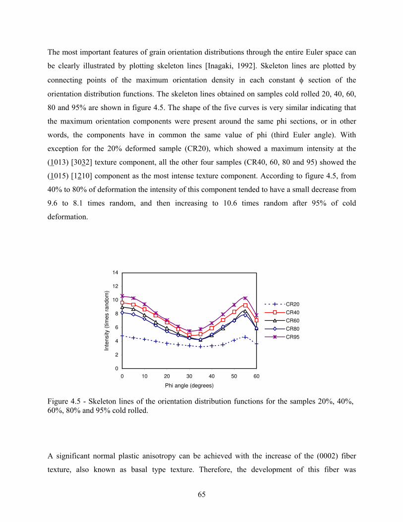
The most important features of grain orientation distributions through the entire Euler space can
be clearly illustrated by plotting skeleton lines [Inagaki, 1992]. Skeleton lines are plotted by
connecting points of the maximum orientation density in each constant φ section of the
orientation distribution functions. The skeleton lines obtained on samples cold rolled 20, 40, 60,
80 and 95% are shown in figure 4.5. The shape of the five curves is very similar indicating that
the maximum orientation components were present around the same phi sections, or in other
words, the components have in common the same value of phi (third Euler angle). With
exception for the 20% deformed sample (CR20), which showed a maximum intensity at the
(1013) [3032] texture component, all the other four samples (CR40, 60, 80 and 95) showed the
(1015) [1210] component as the most intense texture component. According to figure 4.5, from
40% to 80% of deformation the intensity of this component tended to have a small decrease from
9.6 to 8.1 times random, and then increasing to 10.6 times random after 95% of cold
deformation.
0
2
4
6
8
10
12
14
0 10 20 30 40 50 60
Phi angle (degrees)
Inte
nsity (
tim
es r
an
do
m)
CR20
CR40
CR60
CR80
CR95
Figure 4.5 - Skeleton lines of the orientation distribution functions for the samples 20%, 40%, 60%, 80% and 95% cold rolled. A significant normal plastic anisotropy can be achieved with the increase of the (0002) fiber
texture, also known as basal type texture. Therefore, the development of this fiber was
65

investigated after each degree of cold and warm rolling reduction and the results are shown in
figures 4.6 and 4.9 for the cold and warm rolled samples, in that order. According to figure 4.6
after 20% of cold deformation the overall intensity of the (0002) fiber texture decreased and it
continued decreasing as the degree of deformation increased to 40 and 60%. At 80% of
deformation the intensity of this fiber started increasing and after 95% of deformation its
intensity was a little higher but still much lower than the intensity found in the material in its
initial condition (before cold rolling). Figure 4.7, which shows the variation in volume fraction
of the (0002) fiber texture as a function of the degree of cold rolling reduction, corroborates what
was just mentioned. The volume fraction was calculated within 10° of the ideal orientation using
the following equation.
(4.1)( ) ⎟⎟
⎠
⎞⎜⎜⎝
⎛⎟⎠⎞
⎜⎝⎛ +−⎟
⎠⎞
⎜⎝⎛ −Δ= ∑∑∑
2
Δθθcos2
ΔθθcosψΔφφ,θψ,8100
11 ii
ψ θ φif
0002 Fiber
0
0,5
1
1,5
2
2,5
3
0 20 40 60 80
Psi angle (degrees)
Inte
nsity (
tim
es r
andom
)
AR
CR20
CR40
CR60
CR80
CR95
Figure 4.6 - Development of the 0002//ND fiber texture for the as received (AR) and 20%, 40%, 60%, 80% and 95% cold rolled (CR) samples.
66

0002 Fiber
0
0,005
0,01
0,015
0,02
0,025
0 20 40 60 80
Cold Rolling Reduction (%)
Volu
me F
raction
Figure 4.7 - Variation in volume fraction of the 0002//ND fiber texture with degree of cold rolling reduction. The as received material corresponds to the 0% cold rolling reduction. 4.1.3 - Warm Rolled Samples
The pole figures presented in figures 4.8 (a) to (e) show the evolution of the (0002) and
(1010) pole figures after five different rolling reductions at 260°C. At this temperature of
deformation, two (0002) poles are formed towards the RD and these two poles are intensified as
the degree of deformation increases varying from 4 times random after 20% of deformation to 8
times random after 80% of deformation. From the observation of figures 4.8 (a) to (d) one can
see a spreading in the distribution of the (0002) poles towards the transversal direction. After
95% of deformation, the spreading increases and the two poles towards RD that were present in
the previous pole figures no long exist. A couple of poles, this time, towards the TD were formed
after 95% of deformation changing completely the aspect of the (0002) pole figure when
comparing to the pole figure results of the other four warm rolled samples.
The orientation distribution function for the samples rolled at 260°C, illustrated in figure
4.9, shows that the warm rolling has a great effect on the texture formation of titanium sheets. A
formation of a fiber type of texture in the section of φ =0° at θ=20°, can be observed in the WR20
sample where the maximum intensity is at the (1015) [5052] texture component.
67

(0002) Pole figure (1010) Pole figure
(a) WR20
Contours: 1 2 3 4
Contours: 0.5 1 1.5 2
(b) WR40
Contours: 1 2 3 4 5 6
Contours: 0.5 1 1.5 2
(c) WR60
Contours: 1 2 3 4 5 6
Contours: 0.5 1 1.5 2
(d) WR80
Contours: 1 2 4 6 8
Contours: 1 2 3 4
(e) WR95
Contours: 1 2 4 6 8
Contours: 1 2 3 4 5
Figure 4.8 – (0002) and (1010) pole figures of the warm rolled samples
68

θ = 0° θ = 90°
(a) WR20 Contours: 1 2 3 4
ψ = 0°
ψ= 90°
(b) WR40 Contours: 1 2 4 6 8
(c) WR60 Contours: 1 2 3 4 5 6
(d) WR80 Contours: 1 2 4 6 8
(e) WR95 Contours: 1 2 4 6 8 10
Phi= 0.0 Phi=30.0 Figure 4.9 - ODF sections of φ =0° and φ = 30°, Roe notation, for the samples warm rolled at: a) 20%, b) 40%, c) 60%, d) 80% and e) 95%.
69

As the degree of deformation increases this fiber tends to shift towards the (0002) plane
with maximum components 5° away from the (1015)[5052]. After 80% of deformation the
aspect of the fiber starts changing and now the maximum texture component is the (1015)
[1210], with intensity of around 9.0 and 12.0 times random for the samples WR80 and WR95,
respectively. Still in ODF sections of φ =0°, a weak fiber texture around the (2021) plane with
average value of less than 2 times random was formed and it was not influenced by the degree of
deformation. After 40% of deformation a fiber along the (2115) plane, in the section of φ = 30°,
is formed and it is destroyed as the degree of warm rolling increases.
0
2
4
6
8
10
12
14
0 10 20 30 40 50 60
Phi angle (degrees)
Inte
nsity (
tim
es r
an
do
m)
WR20
WR40
WR60
WR80
WR95
Figure 4.10 - Skeleton lines of the orientation distribution functions for the samples 20%, 40%, 60%, 80% and 95% warm rolled.
Figure 4.10 shows the skeleton lines for the 20%, 40%, 60%, 80% and 95% warm rolled
samples. According to this figure, it is possible to observe that for the samples deformed from 20
to 80% the texture components that presented maximum intensity, at each of the constant
sections of the ODFs, had their intensities around the same value, making the skeleton lines of
these referred samples to be rather constant throughout the seven phi sections (φ = 0° to φ = 60°).
After 95% of warm deformation in contrast, the skeleton line of the sample assumed a behavior
70

similar to the skeleton lines of the cold rolled samples (see figure 4.5) where a maximum
intensity at φ = 0° and a minimum intensity at φ = 35° is clearly seen.
The behavior of the (0002) fiber present in the as received material and resultant after
rolling at 260°C is presented in figure 4.11, which shows that the warm rolling tends, in general,
to intensify the fiber as the percentage of deformation increases from 20% to 80%. Figure 4.12
shows the volume fraction of the (0002) fiber calculated within 10° of the ideal orientation. As
also observed from figure 4.12, after 60% of deformation (sample WR60) there is a small drop in
the intensity of the fiber, which increases again after 80% and then decreases after 95% of
deformation (WR95).
0002 Fiber
0
1
2
3
4
5
6
7
8
9
0 20 40 60 80
Psi angle (degrees)
Inte
nsity (
tim
es r
andom
)
AR
WR20
WR40
WR60
WR80
WR95
Figure 4.11 - Development of the 0002//ND fiber texture for the as received (AR) and 20%, 40%, 60%, 80% and 95% warm rolled (WR) samples.
71

0002 Fiber
0
0,02
0,04
0,06
0,08
0 20 40 60 80
Warm Rolling Reduction (%)
Volu
me F
raction
Figure 4.12 - Variation in volume fraction of the (0002)//ND fiber texture with degree of warm rolling reduction. The as received material corresponds to the 0% cold rolling reduction. 4.2 - X-ray Peak Profile Analysis
In this section, it is presented the evolution of the dislocation densities and types obtained
from the X-ray peak profile analysis in commercially pure alpha-titanium deformed by rolling at
260o C for the following rolling reduction levels: 40%, 60% and 80%. The dislocation densities
and the average contrast factor of dislocation for each sample were determined by using Multiple
Whole Profile fitting procedure (MWP) [Ribárik, Ungár and Gubicza, 2001]. In this evaluation,
it is assumed that the peak broadening is caused by the smallness of the coherently scattering
domains and by strain effect arising from the presence of dislocations. As it has been shown in
[Ribárik, Ungár and Gubicza, 2001] for case of hexagonal crystals, the MWP fitting procedure
enables the evaluation of six microstructure parameters:
(a) The dislocation density and arrangement parameter, ρ and M. By definition [Wilkens, 1970],
M is the dislocation arrangement parameter in the Wilkens function, and the value of M gives the
strength of the dipole character of dislocations, i.e., the higher the value of M, the weaker the
dipole character and the screening of the displacement fields of dislocations [Wilkens, 1970],
(b) The median and the variance, m and σ, in the size part of the profiles,
(c) q1 and q2 the parameters of the dislocation contrast factors, as shown in equation (2.4).
Details of the MWP method can be found in [Ribárik, Ungár and Gubicza, 2001]. In the present
study the effect of crystallite size was found to tend to infinity. This is due to the fact that the
72

coherent domain is greater than few μm and in this case the effect of size broadening is
insignificant compared with the distortion effect.
As shown in Chapter 2 the presence of crystallographic texture complicates the
interpretation of peak broadening observations. In an attempt to emulate a random
polycrystalline specimen the strongest diffraction peaks from the three different faces of the
orthogonal sample were mixed to form a full diffraction pattern and used in the MWP evaluation
[Gubicza et al., 2003; Glavicic et al., 2004]. These mixed patterns were then used in the MWP
evaluation. The results for the dislocation densities and the arrangement parameter, M, for the
titanium specimens deformed at 40%, 60% and 80% reduction levels are listed in table 4.1. The
errors of the dislocations densities listed in this table are calculated from the covariance matrix in
the refinement.
Table 4.1 - Dislocation densities and arrangement parameter, M, obtained from MWP evaluation for Ti samples deformed at different reduction levels. Rolling Reduction [%] 40% reduction 60% reduction 80% reduction
M 2.9 1.7 1.1
ρ[1/cm2] 5x10¹⁰ ± 5% 8x10¹⁰ ± 10% 10x1010 ± 7%
The hi fractions of dislocation density with the three Burgers vector types, <a>, <c> and <c+a>,
are shown as a function of deformation level in figure 4.13. The results show that:
I) in the specimen deformed at 40% the <c+a> and <a> dislocations type are
dominating the dislocation population present in the sample;
II) at higher deformation levels <a> type is the dominant dislocation type and the
presence of <c+a> dislocation decrease;
III) at all deformation levels the fraction of <c> dislocations type is marginal.
73

30 40 50 60 70 80
20
40
60
80 a type
c type
c+a typeB
urg
ers
Ve
cto
r P
op
ula
tio
n [
%]
rolling reduction [%]
Figure 4.13 - The hi fractions of the three fundamental Burgers vector types, <a>, <c> and <c+a>, as a function of rolling reduction. Note that in the figure the solutions to equations. (2.8, 2.9 and 2.10), the hi fractions, were transformed in percentages.
Figures 4.14 and 4.15 illustrate the (0002) and (1120) Bragg reflections profiles for all
deformations levels studied here. The difference in broadening is due to the difference in the
dislocations types accumulated in each sample. From figure 4.14 it can be observed that the
broadening of the (0002) reflections is decreasing as the deformation increases. However, figure
4.15 shows that the breadth of (1120) reflections increases as the deformation increases. The two
figures are an illustration of the different contrast effect due to different types of dislocations and
are an indication that the content of dislocations with <a> Burgers vector type increases as the
deformations process increases to higher levels.
74

-0.08 -0.04 0.00 0.04 0.08
0.0
0.2
0.4
0.6
0.8
1.0 (0002) reflection
80% deformation60% deformation
No
rma
lize
d I
nte
nsity
K [1/nm]
40% deformation
Figure 4.14 - The line profiles of (0002) Bragg reflections for different deformations levels. On the x-axes K is given by K=2sinθ/λ, where θ is the Bragg angle and λ is the wavelength of the used radiation.
In accordance to the dislocations slip directions, <a>, <c> and <c+a>, (0001), (2110)
and (2113) pole figures were measured for each titanium sample studied here and the results are
being illustrated in figure 4.16 (a) to (d). The as received material, which exhibits a weak texture,
is also being shown in this figure in order to compare the resultant pole figures before and after
warm rolling deformation. Figure 4.16 (a) shows that the <0001> directions of most of the
crystals are distributed on the plane of ND (normal direction)-RD (rolling direction). When the
sample is rolled to a strain equivalent to 40% of reduction, <0001> directions of the crystals
move close to ND as can be seen in figure 4.16 (b), a trend also observed in figure 4.16 (c) for
the sample rolled to a strain of 60%. In figure 4.16 (d) the split from the ND direction becomes
smaller at a higher strain of 80%. Comparing with <0001>, the evolution of <2110> is not so
complicated. The initial distribution of <2110> is random. At a strain of 40%, the <2110>
direction becomes oriented along the plane of RD-TD. At higher deformation rates the <2110>
75

direction becomes concentrated close to RD, but 5° away. This corresponds to the split shown in
the (0001) pole figures. The (0001) pole figures and (2110) pole figures verify that the <a> type
of slip is dominant during the rolling process. The (2113) pole figures in figure 4.16 show that
the number of crystals with <2113> parallel to RD decreases with the increase of rolling strain.
This is further demonstrated in figure 4.17, which shows the evolution pattern of the distribution
density of crystals whose <0001>, <2110> and <2113> are parallel to the RD.
-0.08 -0.04 0.00 0.04 0.08
0.0
0.2
0.4
0.6
0.8
1.0(11-20) reflection
40% deformation
60% deformation 80% deformation
K [1/nm]
No
rma
lize
d I
nte
nsity
Figure 4.15 - The line profiles of (1120) Bragg reflections for different deformations levels. On the x-axes K is given by K=2sinθ/λ, where θ is the Bragg angle and λ is the wave length of the used radiation.
76

(0001) (2110) (2113)
TD
ND
RD (a)
(b)
(c)
(d)
Figure 4.16 - (2110), (0001) and (2113) pole figures of alpha titanium at a rolling reduction of (a) 0%, (b) 40% (c) 60%, (d) 80%, respectively.
77

It can be observed from figure 4.17 that the distribution density of the RD//<2110> increases
with the strain, while the RD//<2113> decreases and the RD//<0001> is always close to zero.
40 60 80
0.0
0.5
1.0
1.5
rolling reduction (%)
Inte
nsity (
tim
es r
an
do
m)
RD//0001
RD//-2113
RD//-2110
Figure 4.17 - Evolution of intensities of components with RD//2110, RD//0001 and RD//2113, respectively, during rolling reduction. 4.3- Texture Simulation
The simulation of the deformation texture is the closure of the methodology proposed in
this work. In this step the evolution of texture was predicted by means of a self-consistent
approach for the large deformation polycrystal viscoplasticity proposed by Molinari, Canova and
Ahzi [Molinari et al., 1987]. The initial texture, corresponding to the As-received material,
consisted of a file with a set of grains orientations extracted from the SOD file (sample
orientation distribution) obtained from the X-ray data for pole figure measurement using the
routine PoPla (Preferred orientation package Los Alamos). Figure 4.18 shows the (0002) pole
figures of measured (a) and discrete grains file (b) for the as-received sample. The sample axes
78

convention adopted here is rolling direction (RD) parallel to the vertical direction, transversal
direction (TD) parallel to the horizontal direction and normal direction (ND), or normal to the
rolling plane, perpendicular to the plane of the paper (or parallel to a vector outwards the paper
sheet). The polycrystalline aggregate represented by the discrete set of orientations consists of
166 grains representing the initial texture.
(a) (b)
Figure 4.18 – (0002) pole figures for the as-received material: (a) experimental and (b) discrete grains file. Axes convention: RD in the vertical direction and TD in the horizontal direction.
The slip systems reported to be activated in different hexagonal crystals ([Rosi et al.
1956; Grooves and Kelly, 1963; Chin, 1975; Conrad, 1981; Phillipe et all, 1995, Fundenberger et
all, 1997; Salem 2002; Glavicic et al. 2003; Zaefferer, 2003; Kalidindi et al. 2004], are of two
types of slip systems: slip systems with <a> Burgers vector (basal, prismatic and pyramidal) and
slip systems with <c+a> Burgers vector (pyramidal I and II). Since <a> Burgers vector lie in the
basal plane of the hexagonal crystal, glide systems with <a> vector like basal and prismatic
together, comprise only four independent systems. For the same reason, addition of pyramidal
<a> set of slip systems will not supply the missing degree of freedom which is responsible for
accommodate deformations in c-axis direction. For that, additional mechanisms such as twinning
and glide in <c+a> direction are required [Tomé and Kocks, 1985].
79
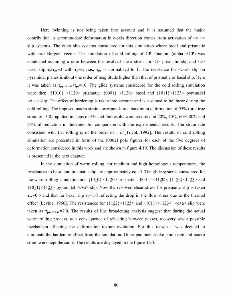
Here twinning is not being taken into account and it is assumed that the major
contribution to accommodate deformation in c-axis direction comes from activation of <c+a>
slip systems. The other slip systems considered for this simulation where basal and prismatic
with <a> Burgers vector. The simulation of cold rolling of CP-Titanium (alpha HCP) was
conducted assuming a ratio between the resolved shear stress for <a> prismatic slip and <a>
basal slip τb/τpr=3 with τp=τ0 ,i.e., τpr is normalized to 1. The resistance for <c+a> slip on
pyramidal planes is about one order of magnitude higher than that of prismatic or basal slip. Here
it was taken as τpyr<c+a>/τpr=10. The glide systems considered for the cold rolling simulation
were then: 1010 <1120> prismatic, 0001 <1120> basal and 1011<1123> pyramidal
<c+a> slip. The effect of hardening is taken into account and is assumed to be linear during the
cold rolling. The imposed macro strain corresponds to a maximum deformation of 95% (or a true
strain of -3.0), applied in steps of 5% and the results were recorded at 20%, 40%, 60% 80% and
95% of reduction in thickness for comparison with the experimental results. The strain rate
consistent with flat rolling is of the order of 1 s-1[Tricot, 1992]. The results of cold rolling
simulation are presented in form of the (0002) pole figures for each of the five degrees of
deformation considered in this work and are shown in figure 4.19. The discussion of these results
is presented in the next chapter.
In the simulation of warm rolling, for medium and high homologous temperatures, the
resistances to basal and prismatic slip are approximately equal. The glide systems considered for
the warm rolling simulation are: 1010 <1120> prismatic, 0001 <1120>, 1122<1123> and
1011<1123> pyramidal <c+a> slip. Now the resolved shear stress for prismatic slip is taken
τpr=0.6 and that for basal slip τb=1.0 reflecting the drop in the flow stress due to the thermal
effect [Levine, 1966]. The resistances for 1122<1123> and 1011<1123> <c+a> slip were
taken as τpyr<c+a>=7.0. The results of line broadening analysis suggest that during the actual
warm rolling process, as a consequence of reheating between passes, recovery was a possible
mechanism affecting the deformation texture evolution. For this reason it was decided to
eliminate the hardening effect from the simulation. Other parameters like strain rate and macro
strain were kept the same. The results are displayed in the figure 4.20.
80

Sample (0002) Experimental (0002) Simulated
(a) CR20
(b) CR40
(c) CR60
(d) CR80
(e) CR95
Figure 4.19 – Experimental and simulated results of the (0002) pole figures for the cold rolled samples deformed (a) 20%, (b) 40%, (c) 60%, (d) 80% and (e) 95%.
81

Sample (0002) Experimental (0002) Simulated
(a) WR20
(b) WR40
(c) WR60
(d) WR80
(e) WR95
Figure 4.20 – Experimental and simulated results of the (0002) pole figures for the warm rolled samples deformed (a) 20%, (b) 40%, (c) 60%, (d) 80% and (e) 95%.
82

CHAPTER 5
DISCUSSION
The texture evolution of cold and warm rolled commercially pure titanium was investigated.
Peak profile analysis of the warm rolled samples deformed at 40%, 60% and 80% was conducted
and simulation of the deformation texture for the samples cold and warm rolled at 20%, 40%,
60%, 80% and 95% was carried out in order to demonstrate the feasibility of the methodology
proposed in this work, which is an unified path model for characterization and also prediction of
microstructure evolution, in terms of texture, in materials that have undergone thermo-
mechanical processing. The results will be reviewed and discussed in this section.
5.1 - Deformation Texture
The texture results for the cold rolled samples shown in figures 4.3 to 4.7 indicate that the
intensity of the (0002) poles almost doubles when the cold reduction increases from 20 to 40%
remaining around the same until the maximum applied cold reduction, 95%. Another effect of
the cold deformation in the distribution of (0002) planes is seen when the degree of reduction
increases to 40% and above. The distribution density of the basal poles towards the rolling
direction decreases and a concentration of these poles tilted ± 20°away from the normal direction
and towards the transversal direction increases with increasing in the degree of cold deformation.
The volume fraction of the basal fiber, (0002)//RD, decreases as the cold reduction increases up
to 60% of deformation. At 80% of deformation the (0002) fiber starts increasing and after 95%
of deformation the sample exhibits volume fraction of (0002) planes, higher than the fraction
observed in the sample 20% cold deformed but still lower than the annealed as received sample.
According to the (0002) pole figures and the profiles of the basal fiber (figures 4.3 and 4.6,
83

respectively), for degrees of cold reduction above 40% the main effect of deformation, rather
than intensification of the basal pole, is the change in the distribution of this pole with regarding
to the normal and the transversal direction of the samples. The main concentration of (0002)
poles tilted ± 20°away from the normal direction and towards the transversal direction of the
sample is very characteristic of cold rolled hexagonal materials with c/a ratios less than the ideal
value of 1.633 as it is the case of titanium [Wang and Huang, 2003]. Keeler and Geisler [Keeler
and Geisler, 1956] working with high purity titanium deformed 99.7% found a tilt of the
hexagonal unit cells in such a manner that the basal planes were rotated 50 ± 10° out of the
rolling plane about the rolling direction. This amount of tilt is much greater than that reported in
this current investigation as well as by earlier investigators [McHargue and Hammond, 1953 and
McGeary and Lustman, 1951]. The reason for that, rather than the high degree of deformation
can be the thermo-mechanical processing and chemical composition of the material.
According to the (1010) pole figure results, the degree of cold rolling reduction do not
affect the intensity of these planes but it plays a role in the distribution of them regarding to the
main sample’s directions (ND, RD and TD). At 20% of cold deformation, the main concentration
of (1010) poles was around the transversal direction of the sample but as the degree of
deformation increased to 40% until 95%, an alignment of the (1010) poles with the rolling
direction started to happen. These results are in agreement with previews results from the
literature [Wang and Huang, 2003].
According to orientation distribution function, figure 4.4, the general aspect of the
crystallographic orientation distribution after cold rolling changed dramatically when compared
to the as received sample. A small percentage of cold reduction, 20%, was able to result in
relative intense texture components, the (1013) [3032] and (1015) [1210], about 4 times random.
As the degree of cold rolling reduction increased, the (1013) [3032] component disappeared and
the (1015) [1210] texture component still presented was intensified after 40% of deformation
reaching about 8 times random, twice as much as its intensity in the CR20 sample. This texture
component remained at this strength until 95% of deformation when its intensity was increased
to 10 times random. The (1015) [1210] component was the most intense texture component in all
four samples that were cold rolled above 40% of deformation. Brandao [Brandao, 1993] found a
close final texture result, (1014) [1210] component, after cold rolling of zircaloy-4 at different
degrees of reduction. The resultant texture after cold rolling has shown to be very dependent
84
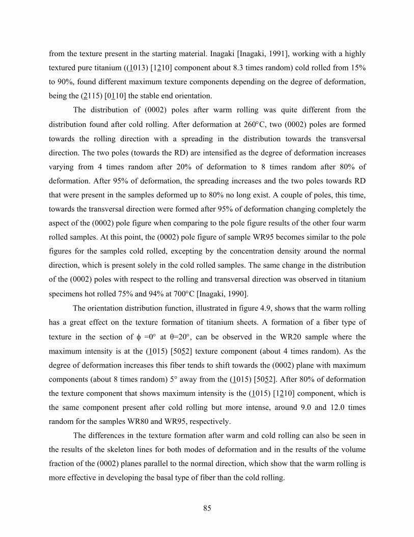
from the texture present in the starting material. Inagaki [Inagaki, 1991], working with a highly
textured pure titanium ((1013) [1210] component about 8.3 times random) cold rolled from 15%
to 90%, found different maximum texture components depending on the degree of deformation,
being the (2115) [0110] the stable end orientation.
The distribution of (0002) poles after warm rolling was quite different from the
distribution found after cold rolling. After deformation at 260°C, two (0002) poles are formed
towards the rolling direction with a spreading in the distribution towards the transversal
direction. The two poles (towards the RD) are intensified as the degree of deformation increases
varying from 4 times random after 20% of deformation to 8 times random after 80% of
deformation. After 95% of deformation, the spreading increases and the two poles towards RD
that were present in the samples deformed up to 80% no long exist. A couple of poles, this time,
towards the transversal direction were formed after 95% of deformation changing completely the
aspect of the (0002) pole figure when comparing to the pole figure results of the other four warm
rolled samples. At this point, the (0002) pole figure of sample WR95 becomes similar to the pole
figures for the samples cold rolled, excepting by the concentration density around the normal
direction, which is present solely in the cold rolled samples. The same change in the distribution
of the (0002) poles with respect to the rolling and transversal direction was observed in titanium
specimens hot rolled 75% and 94% at 700°C [Inagaki, 1990].
The orientation distribution function, illustrated in figure 4.9, shows that the warm rolling
has a great effect on the texture formation of titanium sheets. A formation of a fiber type of
texture in the section of φ =0° at θ=20°, can be observed in the WR20 sample where the
maximum intensity is at the (1015) [5052] texture component (about 4 times random). As the
degree of deformation increases this fiber tends to shift towards the (0002) plane with maximum
components (about 8 times random) 5° away from the (1015) [5052]. After 80% of deformation
the texture component that shows maximum intensity is the (1015) [1210] component, which is
the same component present after cold rolling but more intense, around 9.0 and 12.0 times
random for the samples WR80 and WR95, respectively.
The differences in the texture formation after warm and cold rolling can also be seen in
the results of the skeleton lines for both modes of deformation and in the results of the volume
fraction of the (0002) planes parallel to the normal direction, which show that the warm rolling is
more effective in developing the basal type of fiber than the cold rolling.
85

5.2 - X-Ray Peak Profile Analysis
The results for the dislocation densities and the arrangement parameter, M, for the
titanium specimens warm rolled at 40%, 60% and 80% of deformation, listed in table 4.1,.shows
that the small increment of ρ (dislocation densities) is in accordance with a dynamic recovery
effect, where dislocation annihilation may occur due to the high deformation temperature. The
values of the arrangement parameter M in table 4.1 indicate that the dislocations in the titanium
samples studied here exhibit a week dipole character.
According to figure 4.13, which shows the hi fractions of dislocation density with the
three Burgers vector types, <c>, <a> and <c+a>, it can be noticed that at all degrees of warm
deformation the fraction of the <c> type of dislocation was not significant. The <a> type of
dislocation, on the other hand, was prevalent in all samples and the <c+a> type, although
dominant in sample WR40, decreased its population at higher deformation levels. The results of
the (0001) and (2110) pole figures, shown in figure 4.16, corroborates that the <a> type of slip
is dominant during the rolling process.
The activity of <c+a> dislocations plays an important role in dynamic recovery, as screw
dislocations of <c+a> type can move to the next slip planes by double cross slip followed by
dislocation annihilation. Dislocations with b=<0001> Burgers vector, <c> type, are sessile, thus
its presence can be seen practically unchanged in the deformation range studied here [Jones and
Hutchinson, 1982; Song and Gray, 1995]. The results presented here are in good agreement with
previous extensive TEM studies [Jones and Hutchinson, 1982; Song and Gray, 1995], which
show that the <a> dislocations are the most frequent type of dislocations observed in deformed
titanium and that the <c+a> and <c> types, also reported, are less numerous. The differences in
the broadening of the (0002) and the (1120) reflections (figures 4.14 and 4.15) caused by the
different contrast effect due to different types of dislocations are another indication that the
content of dislocations with <a> Burgers vector type increases as the percentage of deformation
increases to higher levels. The results of the population density of the <c>, <a> and <c+a> types
of dislocation were confirmed through the evaluation of the evolution pattern of the distribution
density of crystals whose <0001>, <2110> and <2113> are parallel to the RD (figure 4.17). From
this figure it can be observed that the <2110>//RD increases with the strain, while the
<2113>//RD decreases and the <0001>//RD is always close to zero. This is in good correlation
with the Burgers vector population results, which show that the density of <a> type of
86

dislocations increases, while the density of <c+a> type of dislocations decreases and <c> type
remains at very low values during the whole rolling process.
5.3 - Self Consistent Simulation of the Deformation Texture
The application of self-consistent approaches for the prediction of cold rolling
deformation textures have been the subject of several investigations [Tomé et al.,1991, Nemat-
Nasser et al., 1999; Schoenfeld et al.,1994; Kalidindi, 1997; Philippe et al., 1995; Funderberger
et al., 1997; Glavicic, 2003]. The most common modes of deformation considered in the
literature for cold working deformation processes are 1010 <1120> prismatic, 0001 <1120>
basal, 1011<1123> pyramidal <c+a> slip and twinning modes. In this work twinning is not
considered and therefore the accommodation of deformation imposed in the c-axis direction is
assumed to entirely done by pyramidal slip with <c+a> Burgers vector. The results shown in
figure 4.19, exhibit a reasonable agreement between experimental pole figures and the respective
predicted ones with small discrepancies on the shape for the higher degrees of deformation
which may be explained by the absence of twinning in the model employed in this work. The
well defined rolling texture of high deformed cold worked hcp metals with c/a<1.663 which is
characteristic of Titanium, a t-type rolling texture presenting a well formed spread in the RD-TD
plane with (0002) poles rotated 35° to 40° from ND towards TD, is explained by the operation of
a combination of prismatic slip and twinning modes. The operation of prismatic and pyramidal
<c+a> slip systems only will tend to push the (0002) poles to form a fiber texture in the outer
rings of the pole figure (for the high deformation case) and the operation of twinning
concomitant with those will tend to stabilize the poles in the described end-stable position for the
cold rolling component of texture. In the other hand if the content of oxygen is high, basal slip
maybe favored and its activation tends to drag the (0002) poles closer to ND as it is the case of
the (0002) pole figures shown in the figure 4.19 (d) and (e).
The TD with angles 15° to 30°, similar to those observed in the (0002) pole figure for the
CR95 sample (figure 4.19(e)). The discrepancies in shape observed in the simulated pole figure
for 95% with a less defined spread towards the rolling direction may be explained by the absence
of twinning in the model. The choice of ratios for the resolved shear stresses of the different
87

systems was based on the findings of previous authors [Tomé et al.,1991, Nemat-Nasser et al.,
1999; Schoenfeld et al.,1994; Kalidindi, 1997; Philippe et al., 1995; Funderberger et al., 1997;
Glavicic, 2003].
In the case of warm rolling the considered slip systems are 1010 <1120> prismatic,
0001 <1120> basal, 1122 <1123> and 1011<1123> pyramidal <c+a> slip. The principal
difference in the approach analysis between warm and cold rolling is the weak contribution of
twinning for the deformation process. At 260°C and higher temperatures up to 700°C twinning is
far less active if not almost completely suppressed in Ti and Zr. and the deformation in the c-axis
direction is accommodated by pyramidal slip with <c+a> Burgers vector in the direction <1123>.
The drop in twinning activity (figure 5.1 ) was also observed by Glavicic [ Glavicic et al., 2004].
Working with the same material, for the range of 20C° to 300C° and 10% reduction, their
observations indicated that the main slip activity over the temperature range investigated was
prism <a> and pyramidal <c+a> type slip.
Figure 5. 1 - Variation of: (a) twin volume fraction; (b) strain accommodated by twinning as a function of rolling temperature.
88

Another evidence that supports the conclusion of low activity of twinning comes from the
observation of optical micrographs of warm rolled samples (figure 5.2).
a) WR80, 200x b) WR95, 200x
Figure 5.2 – Optical micrographs of warm rolled 80% and 95% reduction.
100 μ 100 μ
The results from line-broadening analysis however, have shown a different trend with the
density of <c+a> decreasing with increasing applied strain (figure 4.13). This can be explained
by the high content of oxygen present in the material, situation in which the activation of <c+a>
slip is affected and the fact that at moderate to high temperatures the drop in the resolved shear
stress for both prismatic and basal slip with the ratio between then almost being equal to 1,
favoring a high activity of basal slip 0001 <1120>. This slip activity in the basal plane is also
claimed to be responsible for the rolling texture components being closer to ND, a t-type rolling
texture with (0002) poles rotated 15° to 20° from ND towards TD as it can be observed in the
figure 4.20. The results of simulated deformation texture of warm rolled CP-Ti are in reasonably
good agreement with the experimental results and with the peak profile analysis findings.
89

CHAPTER 6
SUMMARY AND FUTURE WORK
6.1 - Summary
The present work attempts to establish a unified path model for characterization as well
as a prediction of microstructure evolution, in terms of texture, in commercially pure titanium
that have undergone thermo-mechanical processing. Cold and warm at five different degrees of
deformation, 20%, 40%, 60%, 80% and 95% were used in this investigation
The texture evolution of the cold and warm rolled commercially pure titanium samples
was carefully measured. Peak profile analysis of the warm rolled samples deformed at 40%, 60%
and 80% was conducted and simulation of the deformation texture for the samples cold and
warm rolled at 20%, 40%, 60%, 80% and 95% was carried out in order to demonstrate the
feasibility of the methodology proposed in this work, which is an unified path model for
characterization and also prediction of microstructure evolution, in terms of texture, in materials
that have undergone thermo-mechanical processing.
The experimental texture results show that excepting for the samples 95% deformed, the
warm rolling has shown to develop a deformed texture different from the cold rolling.
The results of peak profile analysis carried out for the 40%, 60% and 80% warm rolled
samples show that the <a> type of dislocation was prevalent in all samples while the <c> type of
dislocation was only marginal. The X-ray peak profile analysis, based on the dislocation model
of anisotropic peak broadening, show the dislocation densities, distributions and type during the
rolling processing in good agreement with the texture evolution.
Even though twining was not taken into account during simulation of the cold rolled
samples, there is a reasonable agreement between the experimental and the predicted pole figures
with a small divergence on the distribution of in the TD-RD plane for the higher deformed
samples.
90
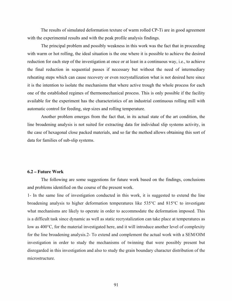
The results of simulated deformation texture of warm rolled CP-Ti are in good agreement
with the experimental results and with the peak profile analysis findings.
The principal problem and possibly weakness in this work was the fact that in proceeding
with warm or hot rolling, the ideal situation is the one where it is possible to achieve the desired
reduction for each step of the investigation at once or at least in a continuous way, i.e., to achieve
the final reduction in sequential passes if necessary but without the need of intermediary
reheating steps which can cause recovery or even recrystallization what is not desired here since
it is the intention to isolate the mechanisms that where active trough the whole process for each
one of the established regimes of thermomechanical process. This is only possible if the facility
available for the experiment has the characteristics of an industrial continuous rolling mill with
automatic control for feeding, step sizes and rolling temperature.
Another problem emerges from the fact that, in its actual state of the art condition, the
line broadening analysis is not suited for extracting data for individual slip systems activity, in
the case of hexagonal close packed materials, and so far the method allows obtaining this sort of
data for families of sub-slip systems.
6.2 – Future Work
The following are some suggestions for future work based on the findings, conclusions
and problems identified on the course of the present work.
1- In the same line of investigation conducted in this work, it is suggested to extend the line
broadening analysis to higher deformation temperatures like 535°C and 815°C to investigate
what mechanisms are likely to operate in order to accommodate the deformation imposed. This
is a difficult task since dynamic as well as static recrystalization can take place at temperatures as
low as 400°C, for the material investigated here, and it will introduce another level of complexity
for the line broadening analysis.2- To extend and complement the actual work with a SEM/OIM
investigation in order to study the mechanisms of twinning that were possibly present but
disregarded in this investigation and also to study the grain boundary character distribution of the
microstructure.
91

3- To incorporate twinning to the actual self-consistent approach. The model for simulation of
deformation texture used in this work was not developed in such way that twinning was taken
into account as a possible mechanism of de formation. In fact, since twinning is not a major
system for the case in study, this self-consistent scheme has proven to render consistent
predictions in both HCP and Cubic materials. However the complete absence of twinning leads
to small discrepancies like those observed in the simulation results for the heavily warm and cold
rolled samples (figure 4.19(e) and 4.20(e)) where the spread observed in the experimental pole
figures was not present in the simulated pole figures.
4- To use better homogenization theories
5- To extend the calculation of the contrast factors to individual slip systems. In the actual stage,
the line broadening approach is capable to predict the activity of individual slip systems in the
case of materials with cubic structure. The extension of the method to predict the activity of
individual slip systems in the case of materials with hexagonal structure would be for sure a great
breakthrough towards better tools and paths for prediction and control of deformation texture of
this important class of materials.
6 - Extension of the self-consistent formulation to the case of bi-modal structure as in the case of
(α+β) titanium alloys.7- To extent the line broadening analysis to (α+β) titanium alloys taking
into account the individual systems activated in the case of both structures and their interaction
as is the case of transformation textures and variant selection problems.
92

REFFERENCES
Ahzi, S. (1987), A Self-Consistent Approach for the Viscoplastic Behavior of Polycrystals Under Large Deformations, PH. D Thesis, Universite de Metz (France). Asaro R.J., Needleman A. (1985), Acta Metallurgica, vol. 33, p. 923. Berveiller M., Zaoui A. (1980), Proceedings of the 15th Colloquium GFR, Paris, p. 175. Bishop J.F.W., Hill R. (1951), Phil. Mag., vol. 42, p. 1298. Bomberger H.B., Froes F.H., Morton P.H. (1985), Titanium technology: present status and future trends, Titanium Development Association, p. 3. Borbely A., Driver J.H, UNGÁR T. (2000), Acta Materialia, vol. 48, p. 2005. Boyer R., Welsch G., Collings E. W. (1994), Materials properties handbook: Titanium alloys, ASM International, Materials Park, OH, p. 311. Brandao L.P.M. (1993), Textura e Propriedades Mecanicas da Liga Zircaloy-4, Doctorate Dissertation, Rio de Janeiro, Brazil. Bunge H. J. (1970), Kristall und Technik, vol. 5, p. 145. Bunge H.J. (1982), Texture Analysis in Materials Science, Butterworth, London. Bunge H.J. (1987), International Metals Review, vol. 32, p.265. Caglioti G., Paoletti A., Ricii F. P. (1958), Nucl. Instrum. Methods, vol. 3, p. 223. Canova G. R., Molinari A., Ahzi S., Adams B. L. (1989), J. Mechanics and Physics of Solids Castelnau O, Francillette H., Bacroix B., Ledensohn R.A. (2001), Journal of Nuclear Materials, vol. 279, p. 14. Cheary R. W., Dooryhee E., Lynch P., Armstrong N., Dligatch S. (2000), Journal of Applied Crystallography, vol. 33, p. 1271.
93

Chin G.Y. (1975), Metallurgical Transactions A, vol. 6, p. 238. Chung and Buessem (1968), Anisotropy in Single Crystal Refractory Compound, edited by F. W. Vahldiek and S. A. Mersol, Plenum, NewYork, vol. 2. Collings E.W. (1994), The Physical Metallurgy of titanium Alloys, ASM, Metals Park, Oh. Conrad H. (1981), Prog. Materials Science, vol. 26, p. 123. Crosby K.E., Mirshams R.A., Pang S.S. (2000), Journal of Materials Science, vol.35, p. 3189. Cullity B.D. (2001), Elements of X-Ray Diffraction, Prentice-Hall, New Jersey. Davies G.S., Goodwill D.J., Kallend J.S. (1971), Journal of Applied Crystallography, vol. 4, p. 193. Dieter G.E. (1986), Mechanical Metallurgy, McGraw-Hill, New York. Dragomir I. C., Li D.S., Castello-Branco G.A., Garmestani H., Snyder R.L., Ribarik G., Ungar T. (2005), Journal of Materials Characterization – In Press.
Dragomir I.C., Ungar T. (2002), Journal of Applied Crystallography, vol. 35B, p. 556. Dragomir I.C., Ungar T., (2002), Powder Diffraction Journal, vol. 17A, p. 104. Dragomir-Cernatescu I., Li D.S., Castello-Branco G.A., Garmestani H., Snyder R.L. (2005), Scripta Materiallia – In Press.
Fjeldly A., Roven H.J. (1996), Acta Materiallia, vol. 44, p. 3497. Froes F. H. (1990), JOM, vol. 42-3, p.16. Fundenberger J.J., Phillippe M.J., Wagner F., Esling C. (1997), Acta Materiallia, vol. 45, No. 10, p. 4041. Glavicic M.G., Salem A.A., Semiatin S.L. (2004), Acta Materialia, vol. 52, p. 647. Groma I., Ungár T., Wilkens S.M. (1988), Journal of Applied Crystallography, vol. 21, p. 47. Groves G.W., Kelly A. (1963), Philosophic Magazine, vol.8, p. 877. Gubicza J., Dragomir I.C., Ribárik G., Baik S.C., Zhu Y.T., Valiev R.Z. and Ungár T., (2003), Zeitschrift für Metallkunde, vol. 94, p. 1185. Gubicza J., Szepvölgyi J., Mohai I., Zsoldos L., Ungar T. (2000), Materials Science and Engineering A, vol. 280, p. 263.
94

Guillaume M.J., Beauvais C., Hocheid B. (1981), Proceedings of ICOTOM 6, Tokyo, p.975. Hill, R. (1965), Journal of Mechanics of Physics and Solids, vol. 13, p. 89. Hill, R. (1967), Journal of Mechanics of Physics and Solids, vol. 15, p. 79. Hirosuke I. (1992), Zeitshchrift fur Metallkunde, vol. 83-1, p. 40. Honeycombe R.W.K. (1984), The Plastic Deformation of Metals”, Edward Arnold Publ. Ltd., London, p. 112. Honneff H., Mecking H. (1978), Textures of Materials, Springer, Berlin. Hosford W.S. Jr., Backofen W.A. (1964), 9th Sagamore Conference, Army material research conference, Syracuse University Press, p.259. Houtte P. (1981), Proc. ICOTOM6, Iron and Steel Inst., Japan, p. 428. Hunter M.A. (1910), J. American Chemical Society, vol. 32, p. 330. Hutchinson J. W. (1970), Proc. R. Soc. Lond. A, vol. 319, p. 247. Hutchinson J. W. (1976), Proc. R. Soc. Lond. A, vol. 348, p. 101. Inagaki H. (1990), Zeitschrift Fur Metallkunde, vol. 4, p. 282. Inagaki H. (1991), Zeitschrift Fur Metallkunde, vol. 10, p. 779. Inagaki H. (1992), Zeitschrift Fur Metallkunde, vol. 83, p. 40. Iwakuma T., Nemat-Nasser S. (1984), Proc. R. Soc. Lond A, vol. 394, p. 87. Jones I.P., Hutchinson W.B. (1981), Acta Metalurgica, vol. 29, p. 951. Kallend J.S, Kocks U.F., Rollett A.D., Wenk H.R. (1991), Materials Science and Engineering A, vol. 132, p. 1. Klimanek P., Kuzel R. Jr. (1988), Journal of Applied Crystallography, vol. 21, p. 59. Kocks U.F. (1998), Texture and Anisotropy: Preferred orientations in polycrystals and their effect on materials properties, Cambridge University Press, U.K. Kocks U.F., Canova G.R. (1981), Deformation of Polycrystals, Riso Natn. Lab., Roskilde, Denmark, p. 35. Kocks U.F., Chandra H. (1982), Acta Metallurgica, vol. 30, p. 695.
95

Krivoglaz M. A. (1996), X-ray and Neutron Diffraction in Non-ideal Crystals, Springer-Verlag, Berlin Heidelberg, New York. Kröner E. (1961), Acta Metallurgica, vol. 9, p. 155. Kröner E. (1972), Statistical Continuum Mechanics, Springer Verlag, Wien. Kuzel R. Jr., Klimanek P. (1989), Journal of Applied Crystallography, vol. 22, p. 299. Kuzel R.Jr., Klimanek P. (1988), Journal of Applied Crystallography, vol. 21, p. 363. Louër D., Auffredic J.P., Langford J.I., Ciosmak D., Niepce J.C. (1983), Journal of Applied Crystallography, vol.16, p. 183. McGeary R.K., Lutsman B. (1952), Journal of Metals, vol. 191, p. 994. McQuillan A.D., McQuillan M.K. (1956), Titanium, Academic Press, New York, Butterworks scientific publications, London. Mizera J., Driver J.H., Jezierska E., Kurzydlowki (1996), Materials Science and Engineering A, vol. 212, p. 94. Mohamed G., Bacroix B. (2000), Acta Materialia, vol. 48, p. 3295. Molinari A., Canova G.R., Ahzi S. (1987), Acta Metallurgica, vol.35, p. 2983. Morris P.R. (1970), Int. J. Engeng. Sci., vol. 8, p.49. Nemat-Nasser S., Guo W. G., Cheng J. Y. (1999), Acta Materialia, vol. 47, No.13, p. 3705. Nemat-Nasser S., Obata M. (1986), Proc. R. Soc. London A, vol.407, p.343. Nye J.F. (1957), Physical Properties of Crystals, their Representation by Tensors and Matrices, Oxford Clarendon Press. Ogdom H.R., Gonser B.W. (1956), Rare Metals Handbook, C. A. Hempel, Reinhold press New York. Pan J., Rice J.R. (1983), Int. J. Solid Struct., vol. 19, No.11, p. 973. Partridge P.G. (1967), Metallurgical Reviews, vol.12, p. 169. Paton N.E., Backofen W.A. (1970), Metallurgical Transactions A, vol. 1, p. 2389. Philippe M.J., Beauvais C., Hocheid B. (1984), Proceedings of ICOTOM 7, p. 519.
96

Philippe M.J., Mellab F.E., Wagner F., Esling C., Hochheid B. (1988), Proceedings of the Sixth World Conference on Titanium, Les Ullis, p. 135. Philippe M.J., Serghat M., Van Houtte, P., Esling, C. (1995), Acta Metallurgica., vol. 43, p. 1619. Phillipe M.J. (1988), La Revue de Metallurgie, p. 1492. Phillipe M.J., Serghat M., van Houtte P. (1995), Acta Metallurgica et Materiallia, vol. 43, p. 1619. Polmear Ii. (1995), Light Alloys-Metallurgy of the Light Metals, John Wiley and Sons, New York. Popa, N.C. (1998), Journal of Applied Crystallogarphy, vol. 31, p. 176. Randle V., Engler O. (2000), Introduction to Texture Analysis: Macrotexture, microtexture and Orientation Mapping, Gordon and Breach Science Publishers. Reed-Hill R.E. (1992), Physical Metallurgy Principals, PWS-Kent Publishing Company, Boston. Reuss A. (1929), Z. Angew. Math. Mech., vol. 9, p. 49. Ribárik G., Ungár T., Gubicza J. (2001), Journal of Applied Crystallography, vol. 34, p.669. Roe, R.J. (1965), Journal of Applied Physics, vol. 36, p. 2024. Rosi F.D., Dube C.A., Alexander B.H. (1953), Transactions of AIME, February, p. 257. Rosi F.D., Perkins F.C., Seigle L.L. (1956), Transactions of AIME, January, p. 115. Sakai T., Fine M.E. (1974), Acta Metallurgica, vol. 22, p. 1359. Salem A., Kalidindi S.R., Doherty R.D. (2002), Scripta Materialia, vol. 46, p. 419. Scardi P., Leoni M. (2004), Diffraction Analysis of the Microstructure of Materials, E.J. Mittemeijer & P. Scardi editors, Berlin, Springer; p. 51. Schoenfeld S.E., Ahzi S., Asaro R.J. (1995), J. Mech. Phys. Solids, vol. 43, No.3, p. 415. Solas D.E., Tomé C.N., Engler O., Wenk H.R. (2001), Acta Materialia, vol. 49, p. 3791. Song S.G., Gray I.I.I.G.T. (1995), Acta Materialia, vol. 43, p. 2339. Stephens P.W. (1999), Journal of Applied Crystallography, vol. 32, p. 281.
97

Stokes A.R., Wilson A.J.C. (1944), I. Proc. Phys. Soc. London, vol. 56, p. 174. Taylor G.I. (1938), J. Institute of Metals, vol. 62, p. 307. Tomé C.N., Kocks U.F. (1985), Acta Metallurgica, vol. 33, No. 4, p. 603. Tomé C.N., Maudin, P.J., Lebensohn, R.A. and Kaschner, G.C. (2001), Acta Materialia, vol. 49, p. 3085. Ungár T, Borbély A. (1996), Applied Physics Letters, vol. 69, p. 3173. Ungár T, Dragomir I, Révész A., Borbély A. (1999), Journal of Applied Crystallography, vol. 32, p. 992. Ungár T. (2004), Scripta Materialia, vol. 51, p. 777. Ungár T., Groma I., Wilkens M. (1989), Journal of Applied Crystallography, vol. 22, p. 26. Ungár T., Tichy G. (1999), Phys. Stat. Sol., vol.171, p. 425 . Voigt W. (1889), Wied. Ann., vol. 38, p. 573. Wang Y.N., Huang J.C. (2003), Materials Chemistry and Physics, vol. 81, p. 11. Warren B.E. (1959), Progress in Metal Physics, vol. 8, p.147. Warren B.E., Averbach B. L. (1950), Journal of Applied Physics, vol. 21, p. 595. Warren, B.E., Averbach B. L. (1952), Journal of Applied Physics, vol. 23, p. 497. Wilkens M. (1970), Fundamental aspects of dislocation theory, J. A. Simmons, R. De Witt and R. Bullough, editors. NBS Spec. Publ., vol. 317, No.2, p. 1195. Wilkens, M. (1970), Physics of state solidi (a), vol. 2, p. 359. Williamson G.K., Hall, W.H. (1953), Acta Metallurgica, vol. 1, p. 22. Wood R.A. (1972), Titanium Alloys Handbook, Metals and Ceramics, Information Center, Battelle, Publication No. MCIC-HB-02, December. Yadav S., Ramesh K. T. (1997), Material Science and Engineering A, vol. 246, p. 265 . Yoo M.H. (1981), Metallurgical Transactions A, vol.12, p. 409. Zaefferer S. (2003), Materials Science and Engineering, vol. A344, p. 20.
98

Zeller R., Dederichs P.H. (1973), Physica Status Solid (b), vol. 55, p.831. Zhu Z.S., Liu R.Y., Yan M.G., Cao C.X. (1997), Journal of Materials Science, vol. 32, p. 5163.
99

BIOGRAPHICAL SKETCH Name: Gilberto Alexandre Castello Branco
Birth: March 19, 1963; Rio de Janeiro, RJ, Brazil
Citzenship: Brazilian
Occupation: Mechanical Engineer
Education: Graduated on the Fall of 1987 with B.Sc. in Industrial Mechanical Engineering at the
Centro Federal de Educação Tecnológica – Celso Suckow da Fonseca, Rio de Janeiro, Brazil;
graduated on the Summer of 1990 with a M.Sc. in Mechanical Engineering at the Military
Institute of Technology, Rio de Janeiro, Brazil. Thesis title: Sistema de posicionamento
automático de um canhão anti-aéreo. Graduated in 1995 with a specialization degree in
Economic Engineering at the Rio de Janeiro State University, Rio de Janeiro, Brazil. Joined the
Florida State University, Tallahassee, Florida, USA, on the Fall of 1999 for Doctorate studies,
and graduated on the Summer of 2005 with a Ph.D. in Mechanical Engineering. Dissertation
title: Effect of Thermo-mechanical Treatment on Texture Evolution of Polycrystalline Alpha
Titanium. Employment: Computer Programmer (1989 - 1991) and Systems Analyst (1991 -
1992) at DataPrev, Rio de Janeiro, Brazil, from 1989 to 1991. Adjunct Professor in the Eletronic
Engineering Department and from 1991 to 1992 in the Applied Mathematics Department at
Severino Sombra University, Vassouras, Rio de Janeiro, Brazil. Assistant professor at Centro
Federal de Educação Tecnológica – CSF- Rio de Janeiro, Brazil, College of Engineering,
Mechanical Engineering Department, from 1994 to 2000. Visiting Professor from 1995 to 1999
in the Mechanical Engineering Department at the Instituto Militar de Engenharia, Rio de Janeiro,
Brazil. Adjunct Professor at Centro Federal de Educação Tecnológica – CSF- Rio de Janeiro,
Brazil, College of Engineering, Mechanical Engineering Department, from 2000 to 2003
(Sabbatical Leave). Research assistant at the National High Magnetic Field Laboratory, Florida
State University from 1999 to 2003. Adjunct professor at Centro Federal de Educação
100

Tecnológica – CSF- Rio de Janeiro, Brazil, College of Engineering, Mechanical Engineering
Department, from 2003 to present.
Professional Experience: Programmer Skills (COBOL, FORTRAN, PASCAL, BASIC,
ALGOL) in Main frame and Personal Computer environments. CAD programmer certified by
AutoDesk. Developed experience in sample preparation for characterization of Titanium alloys,
Interstitial-Free Steels and Silicon Steel samples by X-ray diffraction and Orientation Imaging
Microscopy (OIM). Micro-characterization using Scanning Electron Microscopy (SEM), OIM,
optical microscopy and X-ray diffraction. Texture analysis; magnetic annealing; magnetic
properties measurements and macro, micro and nano-hardness tests. Teaching at Centro Federal
de Educação Tecnológica – CSF, Severino Sombra University and Instituto Militar de
Engenharia, Rio de Janeiro, Brazil.
101