analysis of thermo-mechanical characteristics of the … · analysis of thermo-mechanical...
TRANSCRIPT

1
ANALYSIS OF THERMO-MECHANICAL CHARACTERISTICS OF THE LENS™
PROCESS FOR STEELS USING THE FINITE ELEMENT METHOD
By
Phillip Roger Pratt
A Thesis
Submitted to the Faculty of Mississippi State University
in Partial Fulfillment of the Requirements for the Degree of Master of Science
in Mechanical Engineering in the Department of Mechanical Engineering
Mississippi State, Mississippi
December 2008

2
ANALYSIS OF THERMO-MECHANICAL CHARACTERISTICS OF THE LENS™
PROCESS FOR STEELS USING THE FINITE ELEMENT METHOD
By
Phillip Roger Pratt
Approved:
_____________________________ Sergio D. Felicelli Professor of Mechanical Engineering (Thesis Director)
_____________________________ John T. Berry Professor of Mechanical Engineering (Committee Member)
______________________________ Mark F. Horstemeyer Professor of Mechanical Engineering (Committee Member)
_____________________________ Steven R. Daniewicz Professor of Mechanical Engineering (Graduate Coordinator)
______________________________
Sarah M. RajalaDean of the Bagley College of Engineering

3
Name: Phillip Roger Pratt
Date of Degree: May 2, 2008
Institution: Mississippi State University
Major Field: Mechanical Engineering
Major Professor: Sergio D. Felicelli
Title of Study: ANALYSIS OF THERMO-MECHANICAL CHARACTERISTICS OF THE LENS™ PROCESS FOR STEELS USING THE FINITE ELEMENT METHOD
Pages in Study: 105
Candidate for Degree of Master of Science
Laser Engineered Net Shaping (LENS™) is a rapid-manufacturing procedure that
involves complex thermal, mechanical, and metallurgical interactions. The finite element
method (FEM) may be used to accurately model this process, allowing for optimized
selection of input parameters, and, hence, the fabrication of components with improved
thermo-mechanical properties. In this study the commercial FEM code SYSWELD® is
used to predict the thermal histories and residual stresses generated in LENS™-produced
thin plates of AISI 410 stainless steel built by varying the process parameters laser power
and stage translation speed. The computational results are compared with experimental
measurements for validation, and a parametric study is performed to determine how the
thermo-mechanical properties vary with these parameters. Thermal calculations are also
performed with the code ABAQUS® to evaluate its potential use as a modeling tool for
the LENS™ process.

ii
ACKNOWLEDGEMENTS
The author expresses his sincere gratitude for the assistance and guidance
received through the course of this research. I would like to thank Dr. Sergio Felicelli for
offering me a graduate research assistant position at Mississippi State University and for
his guidance during this study. I would also like to thank Dr. Liang Wang for his
invaluable assistance, as well as David Baker and Kiran Solanki for their technical
support. I would also like to thank Dr. John Berry who gave much needed advice and
direction, as well Dr. Camden Hubbard of Oak Ridge National Laboratory for his
assistance with neutron diffraction measurement. Additionally, I want to thank the
Center for Advanced Vehicular Systems and my team leader, Dr. Paul Wang, for the
resources and opportunities provided to me.

iii
TABLE OF CONTENTS
ACKNOWLEDGEMENTS ................................................................................................ ii
LIST OF TABLES ...............................................................................................................v
LIST OF FIGURES ........................................................................................................... vi
NOMENCLATURE ............................................................................................................x
CHAPTER
1. INTRODUCTION AND LITERATURE REVIEW .........................................1
1.1 Introduction ......................................................................................................1 1.2 Literature Review .............................................................................................5
1.2.1 Experimentally Measured Effects of Process Parameters in LENSTM ....5 1.2.2 Measurement of Residual Stresses in LENSTM .....................................11 1.2.3 Computational Modeling of the LENSTM Process ................................14
1.2.3.1 Thermal Analyses ......................................................................14 1.2.3.2 Coupled Analyses ......................................................................20 1.2.3.3 Process Optimization .................................................................31
2. ANALYSIS OF THIN PLATES PRODUCED BY LENS™ .........................44
2.1 Overview ........................................................................................................44 2.2 Experimentation .............................................................................................45
2.2.1 Introduction ...........................................................................................45 2.2.2 Experimental Procedure ........................................................................47 2.2.3 Results and Analysis .............................................................................54 2.2.4 Conclusions ...........................................................................................65
2.3 Simulation ......................................................................................................67 2.3.1 Modeling with SYSWELD® ................................................................67
2.3.1.1 Introduction ...............................................................................67 2.3.1.2 Theoretical Thermodynamic Model ..........................................67 2.3.1.3 Phase Precipitation Model .........................................................68

iv
2.3.1.4 Theoretical Thermo-Metallurgical Mechanical Model .............69 2.3.1.5 Finite Element Model Development .........................................71 2.3.1.6 Finite Element Model Implementation ......................................71
2.3.1.6.1 Thermal Calculations .................................................71 2.3.1.6.2 Coupled Thermo-Mechanical Calculations ................74
2.3.1.7 Residual Stress ..........................................................................75 2.3.1.8 Conclusions ...............................................................................89
2.3.2 Modeling with ABAQUS® ...................................................................89 2.3.2.1 Introduction ...............................................................................89 2.3.2.2 Theoretical Thermal Model .......................................................91 2.3.2.3 Finite Element Model ................................................................92 2.3.2.4 Model Implementation ..............................................................94 2.3.2.5 Thermal Calculations ................................................................95 2.3.2.6 Results and Comparison with SYSWELD® .............................97
3. CONCLUSION ..............................................................................................100
BIBLIOGRAPHY ............................................................................................................102

v
LIST OF TABLES
Table 1. Sample LENS™ plates of AISI 410 and corresponding input parameters ....46 Table 2. Maximum and average measured zσ in LENS™ plate samples...................63 Table 3. Comparison of chemical compositionsfor AISI 410 and X20Cr13 stainless
steels ..................................................................................................….74

vi
LIST OF FIGURES
Figure 1. Schematic of LENSTM deposition process. .....................................................2 Figure 2. Coordinate system applied to LENSTM thin plates. ......................................5 Figure 3. Temperature distribution in top layer of AISI 316 plate as measured by
Hofmeister et al. for various laser powers from Reference [6]. ................8 Figure 4. Depth of melt pool (mm) in Z-direction for different values of stage speed
(mm/s) and absorbed energy (J/mm) from Reference [8] .........................9 Figure 5. Distribution of gauge volumes for neutron diffraction measurement of
residual stress within LENS™ thin plate of AISI 316 from Reference [11]. ........................................................................................11
Figure 6. Axial stress components along centerlines of AISI 316 thin plate in (a)
Z-direction and (b) Y-direction from Reference [11]. ............................12 Figure 7. Numerical and experimental temperature measured from center of
molten pool in top layer of LENS™ AISI 316 deposit with PL=275W from Reference [15]. ..............................................................17
Figure 8. Temperature measured from center of molten pool in top layer for
various laser powers from Reference [15]. .............................................18 Figure 9. Temperature in direction opposite to laser travel for (a) variable laser
power and (b) variable stage speed from Reference [16]. ......................19 Figure 10. Variation in molten pool size for various laser powers and translation
speed from Reference [19]. .....................................................................23 Figure 11. Distribution of residual stress in deposit/substrate interfacial region of
MONEL 400 thin plate from Reference [19]. .........................................24

vii
Figure 12. Distribution of hardness in AISI 420 plate as function of idle time, Δt from Reference [19]. ...............................................................................27
Figure 13. Maximum measured cooling rate along travel direction from
Reference [20]. ........................................................................................29 Figure 14. Calculated temperature along direction opposite to moving heat source
for 600 W and 2.5 mm/s and corresponding measurements for Sample 4 from Reference [20]. ...............................................................30
Figure 15. Calculated temperature along depth direction for 600 W and 2.5 mm/s
and corresponding measurements for Sample 4 from Reference [20]. ........................................................................................31
Figure 16. Molten pool size of closed-loop and open loop systems at various stages
of deposition from Reference [8]. ...........................................................32 Figure 17. Laser power (PL) used for each layer to maintain molten pool size of
approximately 2 mm at dtdy = 7.62 mm/s. (b) Molten pool size and
temperature distribution during deposition of Layer 2, 4, 6, 8, and 10 when laser at center of plate width from Reference [21]. .......................35
Figure 18. Temperature vs. time at center width of the plate for Layers 1, 3, 5, and
10 from Reference [21]. ..........................................................................36 Figure 19. Cooling rate vs. time at center width of the plate for Layers 1, 3, 5, and
10 from Reference [21]. ..........................................................................37 Figure 20. Applied laser power (PL) used for each layer to maintain molten pool
size of approximately 2 mm at dtdy
=2.5, 7.62, 20.0 mm/s from Reference [21]. ........................................................................................38
Figure 21. Molten pool size and shape at center of plate in Layer 10 at dtdy
= (a) 2.5 mm/s, (b) 7.62 mm/s, (c) 20 mm/s from Reference [21]. ............39

viii
Figure 22. Molten pool size as function of PL and from non-dimensional process map from Reference [22]. .......................................................................41
Figure 23. Maximum residual stress as function of temperature gradient from
Reference [22]. ........................................................................................42 Figure 24. LENS™-produced thin-walled plate of AISI 410. ......................................47 Figure 25. Neutron diffractometry arrangement at HFIR. ............................................48 Figure 26. Diffraction of neutrons from crystalline planes. ..........................................49 Figure 27. Data sampling locations within AISI 410 LENS™ plates. ..........................51 Figure 28. Measurement direction with respect to sample coordinate system. .............52 Figure 29. Stress components as functions of position along (a) Z-axis of plate and
(b) Y-axis of plate for Sample 4. ............................................................55
Figure 30. zσ as function of position along Z-axis of plate for different laser
powers at dtdy
=(a) 2.5 mm/s (b) 4.2 mm/s. ............................................57
Figure 31. zσ as function of position along Y-axis of plate for different laser power
at dtdy
=(a) 2.5 mm/s (b) 4.2 mm/s. .........................................................58 Figure 32. Area fraction of grains of different sizes from plate Sample 4, obtained
by EBSD analysis. ..................................................................................61 Figure 33. Defects observed in AISI 410 LENS™ plate with optical microscopy at
5x magnification. ....................................................................................62
Figure 34. Average measured zσ as function of laser power for both translations speeds. .....................................................................................................65
Figure 35. Computational domain used for LENSTM thin plate thermal analysis. ......71

ix
Figure 36. Value of Qo applied at each deposited layer for dtdy
= 8.5, 4.2, 2.5 mm/s to maintain constant molten pool size. ....................................................73
Figure 37. Calculation scheme for thermal, metallurgical, and mechanical analyses
in SYSWELD®. .....................................................................................75
Figure 38. Distributions of zσ (MPa) in completed 10-layer plates for dtdy
= a) 2.5 mm/s, b) 4.2 mm/s, c) 8.5 mm/s. ..................................................76
Figure 39. zσ and yσ along width of plate at all dtdy
in Layers a) 1, b) 3, c) 5, d) 7 and e) 9. ...........................................................................................78
Figure 40. Distribution of a) zσ and b) yσ along vertical center line for all dtdy
. .......84
Figure 41. Experimental and computational yσ distributions for dtdy
=2.5 mm/s along a) vertical plate axis and b) along width from vertical centerline. ................................................................................................86
Figure 42. Experimental and computational zσ distributions for dtdy
= 4.2 mm/s along a) vertical plate axis and b) along width from vertical centerline. ................................................................................................88
Figure 43. Computational mesh for 10-layer LENS™ thin plate in ABAQUS®. ........93 Figure 44. Comparison of numerical and experimental temperatures measured
from center of molten pool in top layer of LENS™ AISI 316. ..............96 Figure 45. Comparison of molten pool sizes calculated with ABAQUS® and
SYSWELD® for dtdy
= a) 4.2 mm/s and b) 8.5 mm/s. ..........................98

x
NOMENCLATURE
dtdy
Translation velocity of stage
PL Laser power
T Temperature
dtdT Heating/cooling rate
dydT Translation velocity of stage
To Initial temperature
Ta Ambient temperature
Tl Liquidus temperature
Ts Solidus temperature
h Convective heat transfer coefficient
ε Surface emissivity
σ Stefan-Boltzmann constant (5.67e-08 W/m2K4)
k Thermal conductivity
cp Specific heat
A0 Power intensity
Δt Idle time
H Height

xi
hkld
Spacing between crystalline lattice planes
λ Neutron wavelength
2θ Diffraction angle
h, k, l Miller indices
Qr
Diffraction vector
incidentqr
Vector of travel of incident neutrons
diffractedqr
Vector of travel of diffracted neutrons
hklε
Strain in lattice planes with orientation, hkl
od
Average reference lattice spacing for X,Y, and Z directions
hklσ
Stress accompanying lattice strain, hklε
Ehkl Modulus of elasticity in direction normal to hkl plane
σz Component of residual stress in Z-direction
σy Component of residual stress in Y-direction
σx Component of residual stress in X-direction
Lij Latent heat of transformation from phase i to j
Aij Fraction of phase i transformed to j per unit time
Qr(X,Y,Z) Distributed input energy density
Qo Magnitude of energy input density
re Initial radius of laser beam
ri Reduced radius of laser beam

xii
ze Upper plane on which initial radius located
zi Lower plane on which reduced radius located
fi Volume fraction of of phase i
austenitef Volume fraction of austenite
iMf Fraction of martensite after thermal cycle i
oMf Fraction of tempered martensite
iAf
Fraction of retained austenite after thermal cycle i
oAf
Fraction of retained austenite from previous thermal cycle o
Ms Martensite start temperature
Ti Lowest temperature reached in thermal cycle i\
ETotal Total strain
EE Elastic strain
EP Total plastic strain
CPE Classical macroscopic plastic strain
EThm Thermo-metallurgical strain
ETRIP Transformation-induced-plasticity (TRIP) strain
( )Tiyσ Temperature-dependent yield strength of phase i
F(f) Empirical phase-dependent function
σeq Effective stress
Sij Deviatoric stress

xiii
Thm
MAE →Δ Difference in thermal strain between two phases considered
Ayσ Yield strength of austenite (or softer phase in arbitrary case
⎟⎟⎠
⎞⎜⎜⎝
⎛
y
eqhσσ
Nonlinearity function applied if σeq ≥ 0.5σy
( )Tρ Average temperature-dependent density
( )Tcp Average temperature-dependent specific heat
( )Tk Average temperature-dependent thermal conductivity
( )TL Average temperature-dependent latent heat of melting
dt Length of time step
Le Length of element set in direction of laser travel
1
CHAPTER 1
INTRODUCTION AND LITERATURE REVIEW
1.1 Introduction
Laser Engineered Net Shaping (LENS™) is a rapid manufacturing technology
developed by Sandia National Laboratories (SNL) that combines features of powder
injection and laser welding toward component fabrication. Several aspects of LENS™
are similar to those of single-step laser cladding. However, whereas laser cladding is
primarily used to bond metallic coatings to the surfaces of parts that have already been
produced with traditional methods [1], LENS™ involves the complete fabrication of
three-dimensional, solid metallic components through layer by layer deposition of melted
powder metal.
In this process, a laser beam is directed onto the surface of a metallic substrate to
create a molten pool. Powder metal is then propelled by an inert gas, such as argon or
nitrogen through converging nozzles into the molten pool. Depending upon the
alignment of the nozzle focal point with respect to that of laser, then powder is then
melted either mid-stream or as it enters the pool. As the laser source moves away, the
molten material then quickly cools by conduction through the substrate, leaving a
solidified deposit.

2
The substrate is located on a 3 or 5-axis stage capable of translating in the X and
Y-directions. Initially, a 3-D CAD model is created to represent the geometry of a
desired component. The CAD model is then converted to a faceted geometry composed
of multiple slices used to direct the movement of the X-Y stage where each slice
represents a single layer of deposition. During the build, the powder-nozzle/laser/stage
system first traces a 2-D outline of the cross section represented by each slice I the X-Y
plane and then proceeds to fill this area with an operator-specified rastering pattern. The
laser/nozzle assembly then ascends in the Z-direction so that the next layer can be added.
This process is repeated for consecutive layers, until completion of the 3-D component
[2]. This feature is illustrated schematically in Figure 1.
Figure 1. Schematic of LENSTM deposition process.
The ability of LENS™ to manufacture products at near net shape has the potential
to revolutionize the production of small-lot metallic products by decreasing the time and
cost associated with post-process machining. LENS™ can also be implemented to
perform repair operations in situations that would otherwise require fabrication of

3
replacement parts [3]. Furthermore, in a study conducted by Griffith et al . [4] into the
mechanical properties of LENS-deposited™ AISI 316, the researchers recorded a 100%
increase in yield strength over that of the wrought alloy. Griffith et al. [4] theorized that
the improved mechanical performance was derived from a very fine grain structure
measured in the deposited material as a result of the extremely high cooling rates
observed during LENS™ deposition.
A thorough understanding of the thermo-mechanical characteristics inherent
with the LENS™ process could lead to increased quality in LENS™-fabricated products
by a better selection of LENS™ process parameters, thus leading to a wider acceptance
of this technique in the manufacturing industry. The LENS™ process exhibits complex
thermo-mechanical-metallurgical behavior as it involves the laser-induced melting,
solidification, and re-melting of successive layers of powder metal by a moving heat
source, i.e. the laser, in the presence of a large heat sink, i.e. the substrate, as well as other
sources of heat loss, such as that due to convection and radiation. The thermal history
generated during the building of part determines the metallurgical phases present within
the finished product and, hence, its mechanical properties. Thermal strains, metallurgical
transformations, and phase interactions that occur during the process induce residual
stresses that limit the service loads that may be applied to LENS™ products in the field.
Large thermal strains can also lead to geometric distortions that take part dimensions out
of tolerance. The thermo-mechanical-metallurgical properties are heavily dependent
upon the process parameters, i.e. the heat input from the laser, the translation speed of the
X-Y stage, the flow rate of metal powder, and various others. Accordingly, it is
important that computational tools are developed to effectively predict the thermo-

4
mechanical-metallurgical properties of LENS™ parts for any particular combination of
process parameters.
The goals of this study were the generation of a process map for optimal selection
of the parameters laser power and stage speed to limit residual stresses and the
development of computational tools to accurately predict the magnitudes and
distributions of residual stresses in LENSTM-produced components. The development of
a process map involved analyzing experimental measurements of residual stresses in
seven thin plates of AISI 410 stainless steel produced by LENSTM with different values of
laser power and translation speed. The measurements were collected using the neutron
diffraction method. The advancement of a computational tool involved the use of a
coupled thermo-mechanical-metallurgical model to simulate the various physical aspects
of the plate depositions for similar process conditions. The modeling calculations were
performed with the finite element method (FEM), using the welding analysis software
SYSWELD® and the general purpose finite element (FE) package, ABAQUS®. For
verification of accuracy, the numerically predicted residual stresses were then compared
to the measured values, while several calculated thermal characteristics were compared to
corresponding experimental values measured during the depositions of the plates. The
next section presents a comprehensive literature review of previous efforts to relate
process parameters to the thermo-metallurgical characteristics of LENSTM components, as
well as studies involving the measurement of residual stresses in LENSTM deposits.
Additionally, previous efforts to computationally model the process are examined.
For subsequent descriptions of the LENSTM deposition of thin plates and the
related process parameters, the coordinate system shown in Figure 2 will be adopted.

5
Figure 2. Coordinate system applied to LENSTM thin plates.
For the arrangement shown in the figure, “height” refers to Z-directional plate dimension,
while “width” and “depth” refer to Y-directional and X-directional plate dimensions,
respectively.
1.2 Literature Review
1.2.1 Experimentally Measured Effects of Process Parameters in LENSTM
Keicher et al. [5] evaluated the effects of process parameters on multi-layer
deposition of laser-melted powder Inconel® 625 in a process similar to both laser
cladding and LENSTM. The group initially examined various parameters, including laser
irradiance, stage translation speed, powder flow rate, powder particle size, and the size of
LENSTM-deposited thin plate
Substrate
X
Y
Z
6
each Z-directional increment between layers and their effect on heat affected zone (HAZ)
size generated during the build. The HAZ was defined in this study as the melted region
below the surface of the substrate and was examined post-build via metallographic
analysis. The group conducted a substantial number of tests with three variations of six
process parameters. Their initial findings clearly indicated that the dominant parameters
were stage speed (dtdy ) and laser irradiance, defined as the power per unit area directed
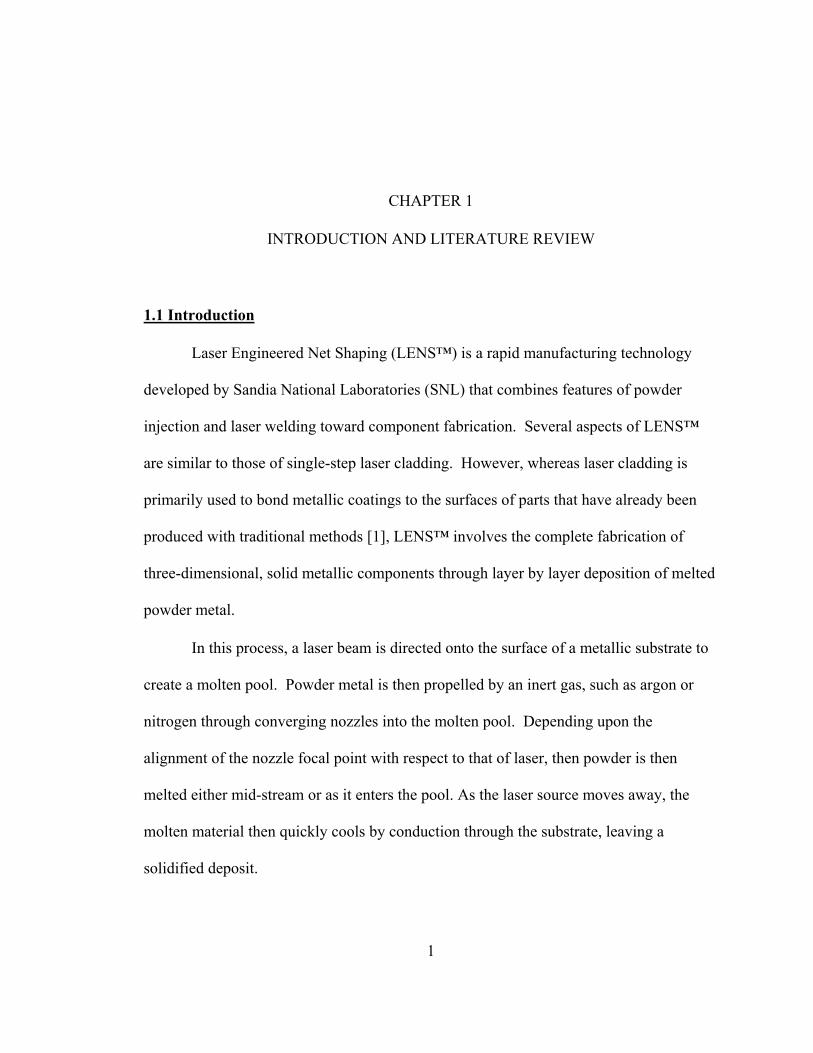
onto a surface by the laser. The tests were performed at laser irradiances of 345, 549, and
774 W/mm2 and =dtdy 8.47, 21.17, and 33.9 mm/s.
The results showed a slight increase in the depth of the HAZ with decreasing dtdy
for each level of irradiance with an approximately 0.05 mm difference between the
maximum and minimum speeds for all irradiances. A larger increase was seen with
increasing irradiance and constant speed, with an approximately 0.1mm difference
recorded between the high and low irradiances for anydtdy . The researchers also
observed a critical input laser power of approximately 220 W after which little no growth
in HAZ occurred.
Hofmeister et al. [6,7] performed in situ experimental measurements of the
temperature distributions in LENS™ thin plates of AISI 316 stainless steel produced with
a range of laser powers (PL) and translation speeds during two studies at SNL. The
purpose of the studies was to calculate the 1-D temperature gradients (dydT ) and cooling

7
rates (dtdT ) in the direction of stage travel (y) from the observed temperature profiles as
f(PL,dtdy ). Thermal imaging was performed with two high-speed CCD cameras. Sample
plates of AISI 316 were produced at laser powers of 212 W, 365 W, and 410 W and
translation speeds of 5.93 mm/s, 7.62 mm/s, and 9.31 mm/s.
After analyzing the thermal images, the group plotted isotherm lines over the
sample plates to observe the distributions of temperatures. In this study, the molten pool
created by the laser was defined as the region with temperature at or above the liquidus of
AISI 316 ( T ≥ 1673K). The group measured 1-D temperature gradients in the direction
of stage travel and calculated the accompanying cooling rates by multiplying the gradient
by the stage speed (dydT
dtdy
dtdT
∗= ) . The researchers found that the highest cooling rates
occurred between the solidus and liquidus isotherms (1645 K < T < 1673 K) and dropped
off slightly at and below the liquidus.
The results showed that the thermal characteristics of a particular build were
strongly dependent on PL anddtdy . Generally, Hofmeister et al. [6,7] found higher
cooling rates (approximately -1000 K/s) between the solidus and liquidus and smaller
molten pool lengths in the Y-direction in cases of low PL, and highdtdy . Conversely,
lower cooling rates (approximately -100 K/s) and larger molten pool lengths were
calculated in cases of high PL, lowdtdy
. The group identified a relationship whereby the
cooling rate is inversely proportional to the square root of the molten pool length. Hofmeister
8
et al. [6,7] concluded that the second case of parameters, which involved higher heat
input, longer heating time, and longer heat sink conduction path, resulted in greater bulk
heating of the sample plates and, thus, shallower temperature gradients at the solid/liquid
interface. Figure 3 is a plot of the recorded temperature as a function of distance from the
molten pool center for various laser powers.
Figure 3. Temperature distribution in top layer of AISI 316 plate as measured by Hofmeister et al. for various laser powers from Reference [6].
Though the molten pool size showed sensitivity to the applied laser power, the
dimensions remained relatively constant above the value of PL = 275 W. Keicher et al.
[5] reported a similar effect whereby the HAZ grew little above PL = 220 W.
A subsequent parametric study by Hofmeister et al. [8] using the same set of
process parameters yielded the results shown in Figure 4.
1550
1600
1650
1700
1750
1800
1850
1900
1950
0 0.2 0.4 0.6 0.8 1 1.2 1.4 1.6
Distance from center of pool (mm)
Tem
pera
ture
(K)
410W 345W 275W 200W 165W

9
Figure 4. Depth of melt pool (mm) in Z-direction for different values of stage speed (mm/s) and absorbed energy (J/mm) from Reference [8]
The pool width in Figure 4 is the depth of the molten pool in the Z-direction, while the
absorbed energy is the product of laser power (PL) and absorptivity (= 0.35) divided by
the stage speed (dtdy ) and the pool width. These results closely match the relationship of
HAZ and speed and heat input to HAZ observed by Keicher et al. [5] for their laser
deposition process.
Yet another study conducted by Smugeresky et al. [9] examined the effects of
process parameters on the measured hardness in thin plates of AISI 316. Using input
laser powers of PL = 150, 300, and 600 W and dtdy = 4.2, 8.5, and 16.9 mm/s, the group
reported a tendency toward higher measured hardness with increasing stage speed for
Absorbed Energy (J/mm)
Pool
Wid
th (m
m)

10
some input power. Also, the hardness appeared to increase with reduction in PL at some
dtdy .
Khalen and Kar [10] performed an investigation into the effects of a several
parameters on the resulting yield strength of AISI 304 stainless steel thin plates in process
identical to LENSTM termed laser-aided direct rapid manufacturing (LADRM). This
team sought to generate a range of input parameter values within which components with
acceptable mechanical properties could be deposited. Their approach involved using the
Buckingham П-Theorem to express the process variables associated with heat transfer
and powder mass flux in terms of 14 dimensionless parameters. Laser power and stage
translation speed were two variables under consideration with experiments values of
P L =300, 400 W and dtdy = 5.1, 7.6, 10.2, 12.7, and 15.2 mm/s examined. The team
recorded temperature profiles during the builds using a pyrometry system and found
larger melt pool sizes and lower cooling rates for PL = 400 W. Additionally, mechanical
testing of the plates after deposition revealed higher yield strengths for cases of
PL = 400 W. These results at first seem contradictory, since the higher cooling rates
observed for cases of PL = 300 W would form finer grained microstructures that should
provide strengthening. However, Khalen and Kar [10] theorized that the larger molten
pools created at higher laser power serve to relieve residual stresses in the previously
deposited layer.
11
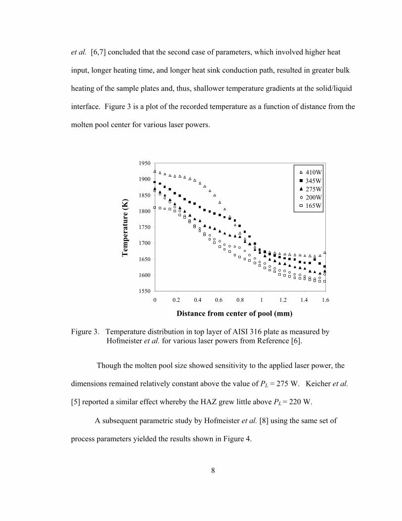
1.2.2 Measurement of Residual Stresses in LENSTM
Rangaswamy et al. [11,12] sought to experimentally measure residual stresses in
LENSTM deposits using the neutron diffraction method, the details of which are discussed
in Section 2.2.2. The measurements were performed on LENS™-produced rectangular
plates of AISI 316. The neutron data was collected at several points methodically
distributed within the geometry of the samples, as shown in Figure 5, to provide a map of
the stress distribution. At these locations the cross-section of entering and exiting
neutron beams created 2.0 mm3 gauge volumes within which elastic strains were
measured.
Figure 5. Distribution of gauge volumes for neutron diffraction measurement of residual stress within LENS™ thin plate of AISI 316 from Reference [11].
Rangaswamy et al. [11] then calculated the axial components of residual stress
through Hooke’s law. Each stress component was then plotted against position within the
plate, first, along the height (Z-direction) on the sample vertical centerline, and next,
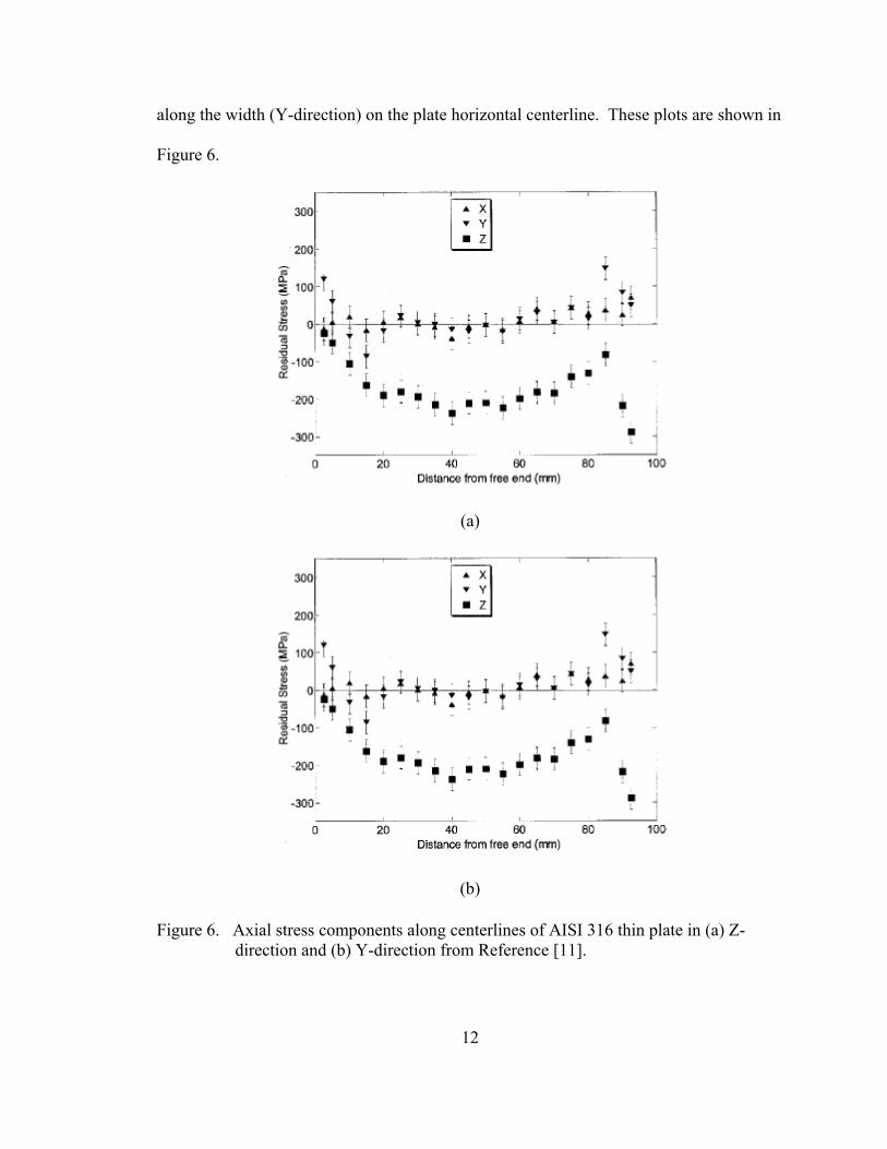
12
along the width (Y-direction) on the plate horizontal centerline. These plots are shown in
Figure 6.
(a)
(b)
Figure 6. Axial stress components along centerlines of AISI 316 thin plate in (a) Z-direction and (b) Y-direction from Reference [11].

13
The results show that the Z-component of stress dominates the stress state within the
plate, which is largely compressive close to the center of the sample. Along the vertical
centerline, the Z-component of stress decreases significantly near the top surface of the
plate, while the Y-component is non-zero at this location. At the other end, closer to the
substrate, the Z-component sharply increases, while the other two components are non-
zero. Rangaswamy et al. [11] attribute the complex stress state at this location to reaction
forces from the substrate and martensitic transformation in the lower deposited layers.
Along the horizontal centerline, the Z-component stresses are compressive near the center
and tensile near the edges. The other two stress components are compressive on one side
of the centerline and tensile on the other. All stress components appear, though, to
balance to an equilibrated state.
In a previous study, Rangaswamy et al. [11] had experimentally determined the
yield strength of LENS™-produced AISI 316 specimens through monotonic tension
testing as 441 MPa. Accordingly, the maximum measured compressive stress within the
thin plate, approximately 215 MPa, represented nearly half the yield of the material.
These measurements show that the residual stress imparted to thin plates during the
LENS™ are substantial and, without the added step of heat treating, would seriously
affect the performance of LENS™ components in the field.

14
1.2.3 Computational Modeling of the LENSTM Process
1.2.3.1 Thermal Analyses
Hofmeister et al. [6] offered some limited finite element calculations in to model
the deposition of a single-pass AISI 316 thin plate. The group modeled the laser melting
as a moving boundary problem for which the solid/liquid interface follows the moving
heat source across the surface being deposited. The boundary problem was solved using
a computationally expensive method that involved the storage of all calculated data at the
end of each time increment followed by the updating of all boundary conditions at the
beginning of the subsequent increment [13]. The deposition of new material was
simulated with an “element birthing” technique, in which new elements were introduced
into the domain at a specified initial temperature. This method has also been termed
“element activation” and has been previously used to model multi-pass welding [14].
The domain represented a plate 25.4 mm wide and 76.2 mm tall composed of
layers one element in thickness. Each new element was introduced into the domain at an
initial temperature of T = 1377 °C (AISI 316 melting point) or T = 1627 °C (case of
superheating) to represent the laser heat source. The only heat transfer mode considered
was conduction through the substrate. The elements were assigned thermal material
properties for a generalized stainless steel. The results showed a steep temperature
gradient near the molten pool which levels to a steady state condition further from the
pool. These results are in agreement with measured data, such as that shown in Figure 3.
However, a detailed parametric investigation was not undertaken.

15
Riqinq et al. [14] also developed a 3-D model for simulating LENSTM deposition
of an AISI 316 thin plate. Their approach was similar to that of Hofmeister et al. [6],
except that the moving solid/liquid interface was reduced to a fixed boundary problem
using an immobilization transformation. The material deposition was accounted for by a
similar element activation method and the laser heat source was represented by setting
the initial temperature of each new element equal to the melting temperature of AISI 316.
As in Reference [6], only conduction heat transfer was considered to occur.
The computational domain was 11mm wide, 6.5 mm tall, and 0.25 mm thick and
composed of 8-node cubic 0.5 mm x 0.25 mm x 0.13 mm elements. Each newly
activated element was held at the melting temperature for the length of time needed to
simulate a 5mm/s stage translation speed. Temperature-independent thermal properties
of AISI 316 were applied to the domain. The computed temperature profiles were
compared to experimental values measured with a two-wavelength pyrometry system for
an AISI 316 thin plate produced with dtdy = 5 mm/s and PL = 240 W. The calculated and
measured temperature profiles showed good agreement with both indicating a sharp
temperature gradient near the solid/liquid interface that dramatically decreased with
distance.
An in-depth study was conducted by Wang and Felicelli [15] who sought to
quantify the effects of varying input parameters and modes of heat transfer in the
LENS™ deposition of a 2-D thin plate of AISI 316 using MULTIA, a research code
generally used to model solidification in castings. For simplicity, only melting of the
final layer was simulated, while the lower layers were assigned a uniform initial
16
temperature obtained from the Hofmeister measurements [6]. The addition of new
elements to the domain was not modeled, but instead the whole top layer was present
throughout the build. The location of the solid/liquid interface was solved in the same
manner as in Reference [6].
Rather than model the heat source as an initial temperature condition, Wang and
Felicelli [15] applied a Gaussian-distributed heat flux load to the top of the plate. They
also applied boundary conditions along top and vertical plate edges to account for losses
due to convection to the chamber atmosphere and radiation emitted from the part. The
latent heat of melting was also included in the governing equation.
In order to validate the accuracy of the model, Wang and Felicelli [15] compared
their calculated results to the findings of Hofmeister and et al. [6] for dtdy
= 7.62 mm/s
and PL = 275 W by simulating the LENS™ deposition of a 10 mm tall, 25 mm long plate
of AISI 316 using input valuesdtdy = 8 mm/s and power intensity of 1.36e06 K/m, which
approximately corresponds to PL = 275 W. The mesh was composed of 100,000 bilinear
square elements 5.0e-2 mm on a side, to which published thermal material properties of
AISI 316 were assigned. The researchers selected a convective heat transfer coefficient,
h = 100 W/m2K, and emissivity, ε = 0.62, to describe the heat losses due to convection
and radiation, respectively. To validate the numerical results, Wang and Felicelli [15]
plotted the simulated temperature as a function of distance from the center of the molten
pool and superimposed the experimental plot shown in Figure 2 for PL = 275 W over his
calculated values. The combined plot, shown in Figure 7, demonstrates good agreement
between the numerical and measured temperature profiles.

17
Figure 7. Numerical and experimental temperature measured from center of molten pool in top layer of LENS™ AISI 316 deposit with PL=275W from Reference [15].
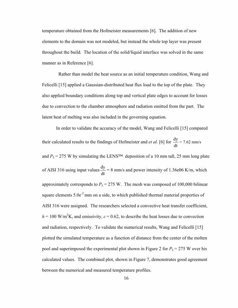
Wang and Felicelli [15] next performed a parametric study similar to that done by
Hofmeister et al. [8] to determine if the same trends in cooling rates and thermal
gradients were observable for different laser power. He repeated the previous simulation
using five power intensity values, revealing that the temperature gradient at the edge of
the molten pool increases substantially with laser power, while the cooling rate decreases.
The resulting plots are shown in Figure 8 where A0 indicates power intensity.
1550
1600
1650
1700
1750
1800
1850
1900
0 0.2 0.4 0.6 0.8 1 1.2 1.4 1.6
Y (mm)
Tem
pera
ture
(K)
Predicted ( 0A =1.3e6 K/m, 0T = bT =1350K)
Measured ( lP =275W) [5]
18
Figure 8. Temperature measured from center of molten pool in top layer for various laser powers from Reference [15].
These same trends were recorded in the experimental study, suggesting that the model
could accurately predict the thermal behavior of LENS™.
A similar study was conducted by Neela and De [16] to study the effects of
translation speed and laser power on the resulting temperature profiles using the general
purpose FE package, ABAQUS® 6.6. The researchers used an element
activation/deactivation similar to those previously seen in References [6] and [14] to
model the deposition of a thin plate of AISI 316 with temperature-dependent thermal
conductivity and specific heat according to a liner, and quadratic relation, respectively.
As in Reference [15], the heat source was described by a Gaussian-distributed heat flux,
which was applied to the domain through the ABAQUS® subroutine DFLUX. Neela and
De [16] simulated the building of a 15 mm wide, 6.25 mm tall, 1 mm thick plate
1.5 1.20.90.3 0.6
Tem
pera
ture
(K)
Y (mm)
19
discretized into a mesh of 25200 8-node, C3D8T heat transfer elements. The process
parameters considered were PL = 165, 200, 275, 345, and 410 W and dtdy = 5-10 mm/s.
Their calculated temperature profiles for an active layer are shown in Figure 9.
Figure 9. Temperature in direction opposite to laser travel for (a) variable laser power and (b) variable stage speed from Reference [16].
Y (mm) (a)
Tem
pera
ture
(K)

20
Figure 9 (Continued).
The predicted trend in Figure 9(a) for increasing PL matches that calculated by Felicelli
and Wang [15], and the relations in both 9 (a) and 9 (b) are supported by the experimental
molten pool data recorded by Hofmeister et al. [8]. The authors noted that any calculated
temperatures greater than 2800 K were not realistic, since the material would boil above
this temperature.
1.2.3.2 Coupled Analyses
Several efforts have been made to relate resultant mechanical properties to the
thermal histories generated during LENS™, as well as in various other laser deposition
processes. Deus and Mazumder [17] attempted to predict the residual stresses resulting
from a laser cladding deposition of C95600 copper alloy onto an AA333 aluminum alloy
Tem
pera
ture
(K)
Y (mm) (b)

21
substrate. Since residual stresses would be generated by the heterogeneous thermal
expansions of the deposited and substrate materials, accurate stress calculations would
also require accurate prediction of the temperature fields created during the build.
Accordingly, Deus and Mazumder [17] developed a 2-D thermo-mechanical model using
the finite element package ABAQUS 5.4. The model implementation did not employ a
direct coupling of thermal and mechanical processes, but rather used the calculated
temperature fields as input for the mechanical constitutive model in a weak-coupling
scheme. As in References [15] and [16], the laser source was described by a Gaussian-
distributed heat flux and material deposition was simulated with an element activation
technique.
The constitutive model used was a simplified temperature-dependent, elastic-
perfectly plastic type, meaning that any strengthening beyond yield the point, which was
determined by a Von Mises criterion, was not considered for either material. Though
Deus and Mazumder [17] recognized the many simplifications used to define the model,
they argued that the calculated results would be qualitatively accurate.
The researchers performed a series of purely heat transfer simulations to
determine a combination of laser power and travel speed that would result in an
acceptable laser clad, i.e. the molten pool extending to the deposit/substrate interface, but
not below it. This condition was achieved with an absorbed laser power of 210 W and a
translation speed of 12.5 mm/s. The resulting stress-strain calculations showed that
plastic strain was generated during the deposition, but that it was restricted to areas where
melting had taken place. Residual stresses in the Z-direction were measured with those
above the deposit/substrate interface having tensile values and those below, compressive.

22
Another thermo-mechanical study was performed by Labudovic et al. [18] to
predict residual stresses in a process identical to LENSTM termed the direct laser metal
powder deposition process. A 3-D coupled model was implemented through the FE
package ANSYS® for the deposition of a 50 mm x 20 mm x 10 mm thin plate of
MONEL 400 onto a substrate of AISI 1006. The deposition was modeled with an
ANSYS® element activation option similar to those already presented. Energy input
density was modeled as a moving Gaussian distribution through the ANSYS® Parametric
Design Language subroutine. The constitutive model was a temperature-dependent
visco-plastic model, in which viscous effects were neglected by ignoring it the associated
term in the equation of state. As in Reference [17], a weak coupling formulation was
used by ANSYS® to approximate the coupled solution.
In order to qualify the thermal calculations, a parametric study was performed to
compare computational and experimental molten pool sizes for various combinations of
input variables. The process parameters used were PL = 400, 600, and 800 W and
dtdy = 5, 10, and 15 mm/s. Experimental measurements were taken using a high shutter
speed camera to capture molten pool size. Additionally, the thermal model was solved
analytically for temperature isotherms and compared to both computed and observed
results. These comparisons are shown in Figure 10.

23
(a)
(b)
Figure 10. Variation in molten pool size for various laser powers and translation speed from Reference [18].
Pool
Wid
th (m
m)
Pool
Wid
th (m
m)
Layer No.
Layer No.
24
Excellent agreement is obtained amongst all three solutions. The relationships between
molten pool size and the input parameters are similar to those already presented in
Figures 8, 9, and 4 from Reference [15], [16] and [8], respectively.
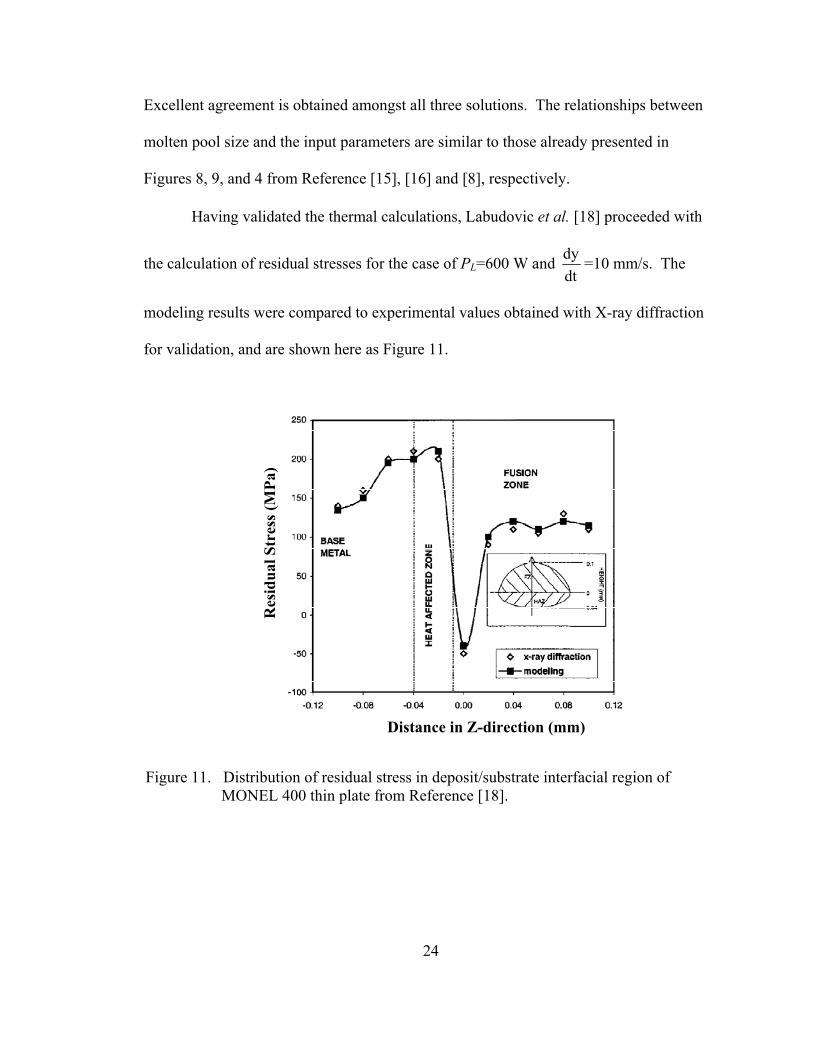
Having validated the thermal calculations, Labudovic et al. [18] proceeded with
the calculation of residual stresses for the case of PL=600 W and dtdy =10 mm/s. The
modeling results were compared to experimental values obtained with X-ray diffraction
for validation, and are shown here as Figure 11.
Figure 11. Distribution of residual stress in deposit/substrate interfacial region of MONEL 400 thin plate from Reference [18].
Res
idua
l Str
ess (
MPa
)
Distance in Z-direction (mm)

25
As with the thermal calculations, the predicted stresses closely match the
experimental values. The weakly coupled thermo-mechanical analysis is capable of
accurately approximating the induced stresses.
Several authors have also attempted to capture the relationship between thermal
and metallurgical processes in laser powder metal deposition, since the resulting
microstructure significantly influences the mechanical properties of the finished part.
Costa et al. [19] performed a series of computational tests to determine the effect on
substrate size and idle time (time between depositions of consecutive layers) on the
resulting thermal histories and subsequent microstructural transformations in laser
powder deposition of thin plates of AISI 420 stainless steel. The goal of the study was to
predict the final distributions of austenite and martensite phases in the plates considering
different substrate masses and idle times.
The group employed a direct coupling formulation for their thermo-metallurgical
model whereby calculated temperature fields were used as input for a semi-empirical
Koïstinen-Marbürger thermo-kinetic model to calculate the proportions of austenite,
martensite, and tempered martensite phases. The calculated phase fractions were then
used to update the thermal properties of the alloy, which were defined as temperature-
dependent weighted averages of the constituent phases. These updated properties
(specific heat, latent heat, thermal conductivity, density) were then used to calculate the
temperature field for the subsequent time step, thereby enacting the direct coupling.
The calculations were performed in ABAQUS® for a 10 mm x 1 mm x 0.5 mm
plate composed of ten deposited layers. As in previous studies, the ABAQUS® element
activation procedure was used to model the deposition, whereby new elements entered

26
the domain with an initial temperature equal to the liquidus of AISI 420. Additionally,
the heat source was defined as a Gaussian-distributed energy input density. The cases
studied all considered PL = 325 W and dtdy = 10 mm/s, while values of Δt, idle time, were
1, 2, 3, 4, 5, and 10 seconds. The substrate masses studied were 13.5 g and 102.8 g.
The thermal results showed a similar cooling effects for large Δt and large
substrate, in which a deposited layer experienced a significant reduction in temperature
prior to the deposition of the next layer. Conversely, small values of Δt or small
substrate, inhibited cooling between layer depositions, and result in comparatively large
molten pool depths that initiated re-melting in previously deposited layers.
The variation in temperature profiles had profound effects on the subsequent
microstructural distributions. For cases of large Δt and/or large substrate, the heated
regions reached sufficient temperatures to induce austenitic transformation, but then
rapidly cooled below the martensite initiation temperature, transforming in a tempered
martensite phase. This process occurred in previously deposited layers as well, causing
successive generations of martensitic tempering in each layer and heterogeneous final
microstructure. For cases of small Δt and/or small substrate, conduction through the
substrate was insufficient to cool below the austenization temperature in the top six
layers. Accordingly, these layers remained austenitic until all ten layers had been
deposited, after which a uniform cooling to room temperature occurred that resulted in 1st
generation martensite microstructure in this region of the plate.
The distribution of hardness in the final part was directly dependent on the phases
present and, accordingly, on the idle time and substrate dimensions used. This

27
dependency is shown in Figure 12, which plots hardness values along the vertical plate
centerline for different idle times and a large substrate.
Figure 12. Distribution of hardness in AISI 420 plate as function of idle time, Δt
from Reference [19].
Wang et al. [20] used a coupled thermo-metallurgical model to predict the
temperature fields in LENSTM-deposited thin plates of X20Cr13 for different values of PL
anddtdy . The modeling results were compared to experimental temperature
measurements taken via radiation pyrometry during LENSTM fabrication of AISI 410 thin
plates using the same process parameter values. The group showed the chemical
composition of the two alloys to be nearly identical and thus valid for comparison.
Computational modeling was performed with the FE software SYSWELD®, an analysis
package designed to perform welding simulations. A coupling scheme similar to that
seen in Reference [19] was used, as well as the same Koïstinen-Marbürger phase
Vic
kers
Har
dnes
s
Distance in Z-direction (mm)
Layer No.
28
transformation model. The phases considered were retained austenite, martensite, and
tempered martensite.
The computational domain represented a 10 mm x 1 mm x 0.5 mm thin plate
composed of ten layers. The deposition was modeled with a “dummy element” method,
in which whole layers were added to the domain at the beginning of the time step
following the completion of the previous layer. Regions of the layer were activated in
response to the location of the heat source through a change of thermal properties,
whereby those elements forming layers yet to be deposited were given excessively low
thermal property values that prevented them from interacting thermally with the
deposited regions. For layers in the process of deposition, elements were assigned the
values of X20Cr13 for some initial volume fraction of phases and allowed to heat up, but
were switched to austenite( 01faustenite .= ) when the austenization temperature of
X20Cr13 was reached. Once austenitized, the elements were considered to be in the
‘deposited’ condition and allowed to undergo phase transformation according to the
kinetic model as they heated and cooled throughout the build process.
Ten experimental samples were deposited with combinations of input parameters,
PL = 300, 450, and 600 W and dtdy = 2.5, 4.2, and 8.5 mm/s. The sample plates each
consisted of 25 single-pass layers. The widths of the plates (Y-direction) varied
somewhat from sample to sample, yet were all within 22-38 mm. The height (Z-
direction) remained constant at 15 mm, while the thicknesses ranged from 1 mm to 3 mm
based upon input parameters – more powder melted at larger laser powers and lower
translation speeds.

29
The corresponding simulations were performed with conical Gaussian-distributed
input energy densities of 300, 450, or 600 W/mm3 and assumed a distribution of 1.0mm3.
The moving heat source was modeled with a SYSWELD® subroutine using the same
values as those in the experimental builds. The heat source moved in the same direction
for each layer and was deactivated between consecutive layer depositions for a specified
idle time, Δt, that depended on the velocity of the source. The computational domain was
chosen to represent an actual plate 25 mm long, the length of several of the samples.
Accordingly, the value of Δt was specified to account for the excluded 15mm of
deposition. Wang et al. [20] proposed that this approximation was valid, since the large
cooling rates measured by thermal pyrometry for the experimental samples indicate that
the heating effects are highly localized. Their measured cooling rates are shown in
Figure 13.
Figure 13. Maximum measured cooling rate along travel direction from Reference [20].
Max
imum
Coo
ling
Rat
e in
Y-D
irec
tion
(°C
/s)
Stage Translation Speed (mm)

30
These extreme levels of cooling suggest that a newly deposited or, newly re-heated,
region of the plate quickly returns to room temperature after moving away from the laser.
The calculated temperature along the direction opposite to that of the moving heat
source is shown in Figure 14 with increasing distance from the center of the molten pool.
The observed distribution in the corresponding experimental sample is also plotted for
comparison.
Figure 14. Calculated temperature along direction opposite to moving heat source for 600 W and 2.5 mm/s and corresponding measurements for Sample 4 from Reference [20].
As shown in Figure 14, the calculated temperature distribution closely matched the
measured values in the direction opposite to the relative travel of the laser. Similarly, the
same temperature change with distance from the center of the molten pool in the Z-
direction, i.e. with increasing depth, is shown for both results in Figure 15.
Tem
pera
ture
(°C
)
Distance from center (mm)
2.5mm/s

31
Figure 15. Calculated temperature along depth direction for 600 W and 2.5 mm/s and
corresponding measurements for Sample 4 from Reference [20].
In both directions, the model closely approximates the change in temperature with
increasing distance from the molten pool center.
1.2.3.3 Process Optimization
Several authors have published studies into the optimization of the LENSTM
process to produce favorable thermal or mechanical properties. Hofmeister et al. [7]
observed via radiation pyrometry that the molten pool increases with height in the
deposition of a thin plate at constant laser power and translation speed as the substrate
and lower layers accumulate heat. The same effect was observed by Wang et al. [20]
both experimentally and numerically, and numerically by Labudovic et al [18].
Hofmeister et al. [7] proceeded to present metallographic results that gave an increased
grain size in the upper layers of an AISI 316 thin plate compared to the lower layers. This
microstructural gradient coincided with decreasing cooling rates and increased molten
Tem
pera
ture
(°C
)
Distance from center (mm)
2.5 mm/s

32
pool size with distance from the substrate, and likely indicates a similar gradient in
mechanical properties. This conclusion is supported by the computational findings of
Costa et al. [19] shown graphically in Figure 12.
In an effort to produce a uniform distribution of microstructure and mechanical
properties throughout the deposited layers, Hofmeister et al. [8] devised a closed-loop
feedback control system that was intended to maintain a steady molten pool size
throughout the deposition process. The feedback controller was incorporated into the
pyrometry system used to measure the thermal phenomena of the deposition. A program
was integrated into the system that reduced the input laser power when the molten pool
area exceeded an operator-specified value. The results shown in Figure 16 compare the
molten pool sizes of cases run with and without the feedback system for the deposition of
a thin-walled square perimeter for advancing periods of the build.
Figure 16. Molten pool size of closed-loop and open loop systems at various stages of deposition from Reference [8].
Isot
herm
al A
rea
(pix
els)
Data Set number
Las
er C
urre
nt (A
)

33
The plot shows that the isothermal area, i.e. the molten pool area detected by the CCD
camera, increases with time throughout the build in the open loop system, which
corresponds to a constant laser power setting. However, the molten area remains nearly
constant when the closed-loop system is implemented. The figure also shows the
decrease in current used by the laser for a closed loop system as the laser power is
decreased with successive depositions. The decline in laser current during the four data
sets represents a 10% decrease in laser power that was required to maintain the specified
molten pool size. Hofmesiter et al. [8] speculated that such a control system would be for
producing consistent and predictable results in LENSTM depositions.
In an effort to model the controlled-loop feedback mechanism presented in
Reference [8], Wang et al. [21] applied sequences of decreasing input energy densities to
generate a steady molten pool throughout the LENSTM deposition of a thin plate. Wang
et al. [21] performed the calculations for the deposition of a ten layer plate in
SYSWELD® using the same mesh presented in Reference [20], as well as the same
boundary and initial conditions. The energy density load was again represented by a
Gaussian function with 1.0 mm3 distribution and the plate material chosen as multi-
phased X20Cr13 stainless steel, for which the thermal properties and continuous cooling
transformation (CCT) diagram were available in the SYSWELD® database.
Wang et al. [21] first considered a deposition at dtdy = 7.62 mm/s, performing
numerous simulations to determine the sequence of energy density settings necessary to
maintain a pool length of approximately 2.0 mm in the Y-direction. Having already
calculated a laser efficiency of approximately 36.4% through comparison of simulated

34
results to the experimental findings of Hofmeister et al. [6], the group found the sequence
of PL that would be used for the build. The sequence and the temperature distributions
for several layers are shown in Figure 17. The size of the molten pool is shown to remain
nearly constant throughout the build, yet some growth can be observed in length (Y-
direction) and depth (Z-direction) as the deposition advances.

35
(a)
(b)
Figure 17. Laser power (PL) used for each layer to maintain molten pool size of
approximately 2 mm at dtdy = 7.62 mm/s. (b) Molten pool size and
temperature distribution during deposition of Layer 2, 4, 6, 8, and 10 when laser at center of plate width from Reference [21].
10 mm
2.0 mm
2
4
6
8
10
300
350
400
450
500
550
600
1 2 3 4 5 6 7 8 9 10
Layer No.
Nom
inal
Las
er P
ower
(W)

36
Tem
pera
ture
(°C
)
The resulting thermal histories for each layer are presented in Figure 18, which is
a plot of temperature vs. time for points located at the centers of Layers 1, 3, 5, and 10
along the vertical plate axis during the entire build process. The plot indicates that the
maximum temperature generated at the midpoint of each layer changes little throughout
the deposition when the optimization scheme is applied. The temperature below which
martensite begins to precipitate is indicated in Figure 18 as Ms = 350 °C. After each laser
pass, the temperature in Layer 1 quickly cools to below Ms only to be heated above it
again during the next pass. Layer 3 shows similar behavior with less cooling, however,
beginning with Layer 5 and continuing to Layer 10, cooling is insufficient to reach Ms.
The plot shows that despite the laser power reduction, the resulting distribution of 1st
generation and tempered martensite will be similar to that predicted by Cost et al. [19].
Figure 18. Temperature vs. time at center width of the plate for Layers 1, 3, 5, and 10 from Reference [21].
0 5 10 15 20
Time (s)
Tem
pera
ture
(°C
)
1st layer 3rd layer 5th layer 10th layer
Ms=350500
0
1000
1500
2000
2500

37
Coo
ling
Rat
e, d
T/dt
, (°C
/s)
Coo
ling
Rat
e, d
T/dt
, (°C
/s)
Wang et al. [21] next plotted the progression of the cooling rates at the plate
center for Layers 1, 3, 5, and 10 through the build process, which is shown in Figure 19.
Figure 19 shows that even though the molten pool remains nearly constant for all layers,
the cooling rates are still significantly reduced for the case of optimized power settings.
Figure 19. Cooling rate vs. time at center width of the plate for Layers 1, 3, 5, and10 from Reference [21].
Wang et al. [21] next applied the molten pool optimization process to the cases of
dtdy = 2.5 mm/s and
dtdy = 20 mm/s to determine the effect of varying the laser translation
speed on the molten pool dimensions. Repeating the previous procedure, Wang et al.
[21] found the necessary sequences to maintain a molten pool length of 2 mm. Figure 20
Time (s)
0 5 10 15 20
3rd layer5th layer
10th layer
Max. cooling rate for each layer Max. cooling rate for 1st layer
1st layer 15000
10000
5000
0
-5000
-10000
1st layer

38
is a plot of for each layer at the three translation speeds. The plot shows that the required
laser power increases withdtdy . The resulting molten pool geometry at the midpoint of
Layer 10 for each value of dtdx is shown in Figure 21. The figure shows that the shape of
the molten pool changes with dtdy , becoming elongated in the Y-direction and shallower
in the Z-direction with higher speed. Accordingly, the model predicts less re-heating of
the previously deposited layers with increased dtdy and the average value of PL for the ten
layers.
Figure 20. Applied laser power (PL) used for each layer to maintain molten pool size of
approximately 2 mm at dtdy =2.5, 7.62, 20.0 mm/s from Reference [21].
200
300
400
500
600
700
800
1 2 3 4 5 6 7 8 9 10
2.5 7.62 20.0
V (mm/s)
Layer No.
Nom
inal
Las
er P
ower
(W)

39
(a)
(b)
(c)
Figure 21. Molten pool size and shape at center of plate in Layer 10 at dtdy = (a) 2.5
mm/s, (b) 7.62 mm/s, (c) 20 mm/s from Reference [21].
Vasinonta et al. [22] sought to create a process map for generating steady molten
pool sizes and limiting residual stress magnitudes. Accordingly, the group performed a
series of weakly-coupled thermo-mechanical analyses using a 2-D FE model to simulate
the heating of a thin plate of AISI 304 stainless steel of some height, H. The mesh was
dtdy = 2.5 mm/s
dtdy = 7.62 mm/s
dtdy = 20.0 mm/s

40
composed of 4-node bilinear elements and calculations were performed using
ABAQUS®. Unlike other studies, Vasinonta et al. [22] chose to model the laser as a
point source rather than a distributed energy density. Additionally, the convection and
radiation were neglected.
Based upon analytical modeling of a moving heat source performed by Rosenthal,
Vasinonta et al. [22] selected three features of the process for non-dimensionalization:
molten pool length, layer height (height of at which deposition is occurring), and melting
temperature. The group then performed a series of thermal simulations with input
parameters PL anddtdy ranging from 43.2 W-165 W and 5.93 mm/s-9.31 mm/s,
respectively. The calculations were performed for temperature-independent material
properties and were used to generate a surface of dimensionless pool length as a function
of dimensionless melting temperature and plate height. The resulting 3-D plot showed a
strong dependence of pool length on melting temperature for all values of non-
dimensional H. A strong dependency on non-dimensional H was only observed for case
of short walls. Based on the non-dimensionalized parameters, which were normalized
with PL anddtdy , Vasinonta et al. [22] predicted values of molten pool size for different
translation speeds and laser powers, as shown. These modeling results are plotted against
experimental data in Figure 22. The plot shows good agreement at all laser powers for
dtdy = 7.62 and 9.31 mm/s, though deviation is seen at
dtdy = 5.93 mm/s.

41
Figure 22. Molten pool size as function of PL and from non-dimensional process map from Reference [22].
The group also developed a non-dimensionalization procedure for temperature
gradient as a function of non-dimensional height and non-dimensional temperature along
the top of the plate. Once again, these variables were described in terms of PL anddtdy .
The generated surface showed a strong dependency of temperature gradient on
temperature along the upper plate edge and, as seen with melt pool length, on non-
dimensional height only for short plates. Vasinonta et al. [22] proceeded with a series of
thermo-mechanical simulations using different PL anddtdy and plotted the ratio of
maximum residual stress magnitude to yield strength as a function of temperature
gradient. The results revealed a strong dependency of residual stress magnitude on the
temperature gradient, which represented the heterogeneous temperature distribution
Mol
ten
pool
leng
th (m
m)
Absorbed Power (W)

42
responsible for thermal strains in the LENSTM. The modeling results are shown in Figure
23 for various values of PL, dtdy , and preheat temperature of the substrate.
Figure 23. Maximum residual stress as function of temperature gradient from Reference [22].
Based on the figure, Vasinonta et al. [22] theorized that two methods exist for
reducing the stress magnitudes. Firstly, reduction of the temperature gradient through
modification of PL anddtdy , and secondly, altering the yield stress of the material through
preheating of the substrate. The plot predicted a 20% decrease in stress for a room
temperature substrate by reducing the temperature gradient and a 40% decrease at
through preheating to 673 K for a temperature gradient of 0.5. Vasinonta et al. [22]
21Z0 0
ZT
.=∂∂ (K/m) x105
Yieldσσmax

43
concluded that the generated process maps could be used for optimizing both the stress
state and molten pools if proper modification of PL and dtdy are considered.

44
CHAPTER 2
ANALYSIS OF THIN PLATES PRODUCED BY LENS™
2.1 Overview
In order to select the appropriate values of the process parameters, laser power
and translation speed needed to minimize residual stresses in LENSTM components, their
relationships must be better understood. Rangaswamy et al. [11,12] measured the
residual stresses at several locations within LENSTM thin plates using neutron diffraction,
while Labudovic et al. [18] used X-ray diffraction to measure the stresses near the
deposit/substrate interface for a LENSTM plate deposit. However, neither of these studies
examined the role of process parameters in determining the stress magnitudes or
distributions. Furthermore, Vasinonta et al. [22] restricted their measurements to the
lower regions of the plate and selected a measurement technique, X-ray diffraction,
which is only capable of nanometer scale penetration into the material.
Accordingly, the effort presented here involves measurement by neutron
diffraction of LENSTM-deposited thin plates of AISI 410 stainless steel produced using
different combinations of laser power and translation speed. The distributions and the
magnitudes of the internal stresses were analyzed to determine if a process map can be
generated for optimizing the selection of values for these inputs. Furthermore, the
experimental data were compared with numerical results to qualify a FE model developed
45
for predicted residual stresses in LENSTM thin plates. The computational simulations
were performed with SYSWELD® using a coupled thermo-mechanical-metallurgical
model and the mesh presented by Wang et al. [20].
Additionally, a multi-phase internal state variable model that may provide better
accuracy for the prediction of residual stresses is presented. Since this constitutive model
cannot be easily implemented in SYSWELD®, the experimental plate depositions are
simulated with a thermal model using ABAQUS® 6.7. These results were compared to
the SYSWELD® calculations, as well as to experimental thermal data from collected by
Wang et al. [20] to verify the use of ABAQUS® for modeling LENSTM.
2.2 Experimentation
2.2.1 Introduction
In order to relate the resulting residual stresses from the LENS™ build process to
the process parameters laser power and stage translation speed, seven of the ten AISI 410
stainless steel thin plates presented by Wang et al. [20] are selected for stress
measurement. The plates were fabricated at the facilities of Optomec®, a private
company specializing in LENS™ manufacturing and repair, using a LENS™ 850M
machine. This machine is equipped with a 3kW IPG laser and a 5-axis stage for part
deposition. The process parameters used in the building of each plate are shown in
Table 1.

46
Table 1. Sample LENS™ plates of AISI 410 and corresponding input parameters.
No. Laser Power
(W)
Laser Speed
(mm/sec)
Length of Part
(mm)
Powder Flow Rate
(cm3/sec)
1 300 2.5 38.1 37.85
2 300 2.5 22.1 37.85
3 300 4.2 25.4 50.47
4 600 2.5 25.4 37.85
5 600 4.2 25.4 44.16
6 450 2.5 25.4 37.85
7 450 4.2 25.4 50.47
8 300 8.5 38.1 88.3
9 450 8.5 38.1 82.01
10 600 8.5 38.1 88.3
The sample plates each consisted of 25 single-pass layers. The widths of the
plates (Y-direction) varied somewhat from sample to sample, yet were all within 22-
38mm. The height (Z-direction) remained constant at 15 mm, while the thicknesses
ranged from 1 mm to 3 mm based upon process parameters – larger laser powers and
lower travel speeds melt more powder. A representative sample plate is shown in Figure
24.

47
Figure 24. LENS™-produced thin-walled plate of AISI 410.
2.2.2 Experimental Procedure
Several methods are available for determining residual stress, such as holographic
interferometry by hole-drilling, the contour method, and X-ray diffraction. However, in
most cases such methods are destructive in nature or are only capable of measuring stress
close to free surfaces. Neutron diffraction, however, a long established measurement
technique, is capable of deep penetration into solid materials for stress determination in a
nondestructive fashion. Accordingly, this option was chosen to measure the stress
distribution within the LENS™ AISI 410. Due to limited availability of the diffraction
instrumentation, only seven of the ten plates produced by Wang et al. [20] could be
measured.
The neutron diffraction measurements were performed at the High Flux Isotope
Reactor (HFIR) facility at Oak Ridge National Laboratory on the NSFR2 diffractometer.
The neutron diffractometry system at HFIR, shown in Figure 25, makes use of a single
15mm
21mm

48
crystal silicon monochromator that selects neutrons of a particular wavelength
(monochromatic) from the reactor stream to bombard the measured sample.
Figure 25. Neutron diffractometry arrangement at HFIR.
Upon contacting the sample material, some neutrons are diffracted by crystalline
lattice planes of a certain orientation that is dependent on the selected neutron
wavelength. If the path difference of the particles as they diffract from different
individual planes is some integer of the wavelength, the neutrons interfere constructively,
and the intensity peak is recorded by seven detectors arranged from -15 ° to +15 ° out of
the horizontal plane of diffraction. The NSFR2 peak fitting program then determines the

49
angle of diffraction, 2θ, by plotting a Gaussian distribution of neutron count vs. angle.
The program then calculates the spacing between crystalline lattice planes, hkld , through
Bragg’s Law of Diffraction, shown here as Equation 1 [23].
θλ sinhkld2=
The diffracting lattice planes in this process are those with plane normals parallel to the
scattering vector, Qr
, which is defined in Equation 2 [10].
diffractedincident qqQ rrr−=
The diffraction process is shown in Figure 26.
Figure 26. Diffraction of neutrons from crystalline planes.
In the measurement of the LENS™ plates, the {330} planes of the silicon
monochormator were selected to diffract neutrons of 1.73 Å wavelength that were then
directed onto the sample plates. The measured diffraction angle of the detected neutrons
after contacting the sample was approximately 94.6 °. In order to determine what
(1)
(2)

50
orientation {hkl} of lattice planes within the sample material was diffracting, X-ray
diffraction was performed on a representative plate sample. In this procedure,
monochromatic X-rays of λ≈1.5 Å were directed onto the polished surface of the plate,
resulting in a high intensity peak at an angle of approximately 90 °. The measured
diffraction profile was referenced against a database of profiles for various materials and
was found to closely match that of iron for which the {211} planes diffract at 2θ ≈ 90 °.
Accordingly, the {211} planes were determined to be those diffracting for AISI 410.
In order to determine how the internal stress varied with position within the
sample plates, several locations were selected for the placement of gauge volumes, 3-D
data sampling regions created by the intersection of the incident and diffracted neutron
beams. The values of hkld calculated from 2θ measurements at these sites would be
averaged throughout the gauge volumes to obtain a single value for each selected
location. The dimensions of the gauge volumes were determined by those of the incident
and diffraction collimator slits through which the neutrons passed before and after
contacting the sample, respectively. The need to fully embed the gauge volumes within
the geometry of the thin plates required small slit sizes that resulted in rectangular shaped
volumes of approximately 2.5 mm3.
The arrangement of the gauge volumes, show in Figure 27, closely matches that
used by Rangaswamy et al. [11], shown in Figure 5, with seven volumes equally spaced
along the vertical (Z-direction) centerline of each plate and four volumes along the
horizontal (Y-direction) centerlines. However, in the case of two of the samples (1,4),
nine volumes were used vertically and six horizontally.

51
Figure 27. Data sampling locations within AISI 410 LENS™ plates.
The measurements were taken at count times of 6-35 minutes and were performed
three times at each gauge volume. Before each repetition, the sample was oriented to
align the scattering vector, Qr
, with one of the three orthogonal directions of the sample
coordinate system (X,Y,Z) in order to measure the average value of hkld in that direction.
In order to convert the recorded lattice spacing values into strains, a strain-free
reference value of hkld was required. Therefore, a coupon was cut from another
LENS™ AISI 410 plate to be measured along with each test sample. Once cut, the elastic
strains in the coupon relaxed so that the measured lattice spacing, od , represented an
unstrained, initial state. The elastic strains were then calculated for the X, Y, and Z
directions through Equation 3 [25].
o
oihklihkl d
dd −= ,
,ε
where i = X, Y, Z
∑=i
ioo d31d ,
Z Y X
Z
(3)

52
In order to avoid the propagation of systematic errors in 2θ measurement into the
hklε calculations, the values of od and hkld for each sample were taken during the same
experimental run, so that such errors would cancel in Equation 3. Additionally, to reduce
the impact of random errors on the strain calculations, replicate measurements of od were
taken during each run. Furthermore, to account for any differences in the value of iod ,
for different directions resulting from any plastic deformation that might be present, the
average reference lattice spacing, od , is used instead. The presence of plasticity in the
LENSTM material and the error in recorded od values is discussed in more detail in
Section 2.2.3.
The relation of the measurement directions to the coordinate system of the sample
is expressed by the angles ψ and φ as shown in Figure 28.
Figure 28. Measurement direction with respect to sample coordinate system.

53
As such, an alternative form of Equation 3 that represents the strain in the measurement
direction in terms of the components of the 2nd order strain tensor is given in Equation 4
[25].
ψφεψφεψφεψεψφεψφεεϕψ 222 23132
122
3322
2222
11 sinsinsincossinsincossinsinsincos +++++=
By aligning the scattering vector Q
rwith the orthogonal axes of the LENS™ plates, those
values of strain calculated with Equation 3 in the X, Y, and Z directions correspond to
oo 900 ,ε , oo 9090 ,
ε , and oo 00 ,ε respectively, in Equation 4. Accordingly, in these
directions ϕψε reduces to 11ε , 22ε , and 33ε , i.e. the principal strains.
Once the principal elastic strains had been determined at all measurement sites,
the corresponding principal stresses were calculated using Hooke’s Law, shown in
Equation 5 [25].
( )( )
( )( )hklhkl
kjihklhkl
hkl
ihklhklihkl 211
E1
Eνν
εεεν
νε
σ−+
+++
+= ,
,
The terms hklE and hklν are the elastic constants corresponding to Young’s
modulus and Poisson’s ratio in the direction normal to the {211} planes. The values of
these terms were found using an algorithm developed by Behnken and Hauk [26] for
calculating {hkl}-specific elastic response for polycrystals from the single crystal
compliance tensor of a material. Since no such compliance data was available in the
literature for AISI 410 single crystals, values of α ferrite compliances recorded by Dever
[27] were used instead. The Behnken-Hauk algorithm is based on a polycrystalline
elastic model developed by Kröner [28] which assumes a random grain orientation is
(5)
(4)

54
present within the material under consideration. The applicability of this model to the
LENS™ plates was verified through the neutron measurements for which no change in
diffracted intensity was detected that would be indicative of a significant texture in the
deposited material.
2.2.3 Results and Analysis
Initial data retrieval revealed that the Debye ring, the profile created by the
diffracted neutrons as they contact the detectors, was not well defined, indicating that the
number of grains in the sample material contributing to diffraction was low. In order to
avoid the random errors in hkld that would result from the poor grain statistics, an
omega oscillation was performed whereby the sample was rotated through an angular
range of -4° to +4° out of the plane normal to the incoming beam to increase the number
of diffracting grains. This procedure was unable to correct the Debye ring profile
completely, but did significantly improve the quality.
Based upon the stress vs. position plots produced for the Rangaswamy et al. [11],
which indicated that the stresses in the X (normal) and Y (transverse) directions were
almost negligible over most of the sample, and the limited time available for
measurements at the HFIR facility, the data was recorded almost exclusively in the
sample Z direction (longitudinal). In order to validate this decision, measurements of
Sample 4 were performed in all three directions. The calculated orthogonal stresses for
Sample 4 are shown in Figure 30 (a) and (b), where the “free end” in Figure 29 (a) refers
to the last deposited layer of material, i.e. the top of the plate.

55
Figure 29. Stress components as functions of position along (a) Z-axis of plate and (b) Y-axis of plate for Sample 4.
The plots in Figure 29 show the stress distribution along the vertical and horizontal plate
centerlines with data points corresponding to the arrangement shown in Figure 27.
-500
-400
-300
-200
-100
0
100
0 5 10 15
Normal
Longitudinal
Transverse
-700-600-500-400-300-200-100
0100200300
-15 -10 -5 0 5 10 15
Normal
Longitudinal
Transverse
Res
idua
l str
ess (
MPa
)
Distance from free end along Z-axis (mm)
(a)
(b) Distance from center along Y-axis (mm)
Res
idua
l str
ess (
MPa
)

56
Contrary to the findings presented by Rangaswamy et al. [11], the magnitudes of the X
and Y stress components, xσ and yσ , are here found here to be reasonably large, ranging
from 50-200 MPa. However, these stresses are still comparatively small enough in
relation to zσ that the decision to restrict measurements to the Z-direction was
reasonable in consideration of the time constraints. The resulting Z-component of stress,
zσ , along vertical and horizontal plate centerlines are shown for each sample in Figures
30 and 31.

57
(a)
(b)
Figure 30. zσ as function of position along Z-axis of plate for different laser powers
at dtdy =(a) 2.5 mm/s (b) 4.2 mm/s.
-250
-200
-150
-100
-50
0
50
-1 1 3 5 7 9 11 13 15
dtdy
=4.2 mm/s
Distance from free end along Z-axis (mm)
Z-C
ompo
nent
Res
idua
l Str
ess (
MPa
) 300 W (#1) 300 W (#2)
600 W (#4) 450 W (#6)
Z-C
ompo
nent
Res
idua
l Str
ess (
MPa
)
Distance from center along Y-axis (mm)
600 W (#5)
450 W (#7)
300 W (#3)

58
Figure 31. zσ as function of position along Y-axis of plate for different laser power at
dtdy =(a) 2.5 mm/s (b) 4.2 mm/s.
-700
-600
-500
-400
-300
-200
-100
0
100
200
-15 -10 -5 0 5 10 15
-300
-200
-100
0
100
200
300
400
-10 -5 0 5 10
dtdy
=2.5 mm/s
Distance from free end along Z-axis (mm)
(a)
Z-C
ompo
nent
Res
idua
l Str
ess (
MPa
) Z
-Com
pone
nt R
esid
ual S
tres
s (M
Pa)
Distance from center along Y-axis (mm)
(b)
dtdy
=4.2 mm/s
300 W (#1) 300 W (#2)
600 W (#4)
450 W (#6)
600 W (#5) 450 W (#7) 300 W (#3)

59
The error in calculated stress, shown as bars at each data point in the figures, was
obtained by propagation of the random error in 2θ and do measurement through
Equations 1, 3, and 5. The random 2θ error was determined by the NSFR2 peak fitting
program, while that for do was determined through replicate measurements taken during
each measurement run. An uncertainty analysis of the do values for each sample
produced a root-mean square deviation from the average ranging from 5 x 10⁻⁵ to 4 x 10⁻⁴
Å. An extremely large error in stress is shown in Figures 29 (a) and 30 (a) at the third
gage volume from the free end for Sample 4. A comparison with the raw data revealed a
similarly large variance of 2θ at this location, which may be due to the presence of a large
grain or some type of defect within the gauge volume that interrupted the uniformity of
the Debye profile across the seven neutron detectors and produce an artificial shift in the
Gaussian curve.
Sources of uncertainty in the magnitudes of the stress calculations that were not
considered when calculating the error shown in the plots were the choice in elastic
constants and plastic strain in the material. Firstly, the elastic constants used in
Equation 5, hklE and hklν , were calculated from single crystal compliances for α ferrite,
which are likely somewhat different from those of a martensitic steel like AISI 410.
However, since no such constants could be found in the literature for AISI 410 or any
other martensitic steels, no direct comparison to α ferrite elastic properties could be made
and the amount of variation is unknown. Another possible source of error in the stress
magnitudes arises from the presence of plastic deformation. Since plastic and elastic
strains cannot be differentiated in the neutron measurements, all lattice deformation
greater than that measured within the reference coupon is taken to be elastic strain in

60
Equation 5. If an equal degree of plasticity exists within the all of the plates and the
reference coupon, then its effects would be negated in Equation 3. However, if the
amount of plastic deformation varied with the processing conditions from sample to
sample, then inaccuracies in the calculated stress fields would be introduced in Equation
3 from this non-uniformity. The value of iod , was averaged amongst the three directions
in Equation 3 in order to reduce any directionally-dependent plasticity effects, i.e.
varying degrees of plastic deformation in the X, Y, and Z-directions, and obtain a value
that was more representative of a strain-free state.
Part (a) of Figures 30 and 31 show that the longitudinal stress is mostly
compressive along the vertical axis of each plate. Some variation in the stress profiles is
observed amongst the different plates; for instance, Samples 1 and 2 show zσ increasing
with distance from farther from the free end, while Samples 3, 4, 5, and 6 show the stress
magnitude reaching a maximum near the plate centers and then decreasing closer to the
plate bottom. For Sample 7, however, zσ is a maximum near the free end, while
continuously decreasing with distance in the direction of the substrate.
Part (b) of Figures 30 and 31 also show zσ generally reaching a maximum near
the plate center and decreasing with distance on either side. Sample 5, which shows a
tensile stress at the center, is an exception, however, a large uncertainty is calculated at
this data point, so this may not be a true deviation from the observed trend. The
corresponding plot from Rangaswamy et al. [11], shown in Figure 6 (b), also shows zσ
to be compressive near the plate center, but then becoming tensile on either side. Since a
balanced state of stress exists within the plates, zσ must necessarily be tensile near the

61
outer surfaces of the samples. By locating their extreme gauge volumes closer to the
outer edges of the plates, Rangaswamy et al. [11,12] were able to capture this transition,
which was only recorded for Sample 1 of this study, shown in Figure 31 (a).
For some cases, such as Sample 1 in Figure 30 (a) and Sample 4 in Figure 31 (a)
substantial peaks are seen in the distributions that interrupt the general trends toward
increasing or decreasing values of zσ . Such peaks could be attributable to grain size
affects where grains with dimensions on the order of those of the gauge volumes generate
shifts in the Gaussian profile. In order to determine if this was the case, several of the
sample plates were mounted and polished so that electron back scatter diffraction (EBSD)
could be deformed. The EBSD scans were performed at the Center for Advanced
Vehicular Systems at Mississippi State University using a SUPRA 40 FEG scanning
electron microscope (SEM). The EBSD analysis produced grain size distributions, such
as that shown in Figure 32, at several locations within the sample plates.
Figure 32. Area fraction of grains of different sizes from plate Sample 4, obtained by EBSD analysis.
Grain Size (Area) [μm2]
Are
a Fr
actio
n

62
Figure 32 shows that approximately 90% of the grains at the measurement location have
a cross sectional area of less than 10μm2, which is significantly less than the cross
sectional area of the incoming neutron beam, 3.5 mm2. These results show that LENS™
material has a very fine grain structure and that the observed peaks are likely not caused
by the boundaries of large grains intersecting the sample volumes. In order to determine
if other defects were present in the material, the polished samples were examined with
optical microscopy. Observation of one of the samples revealed large objects, such as
those shown in Figure 33, some of which were approximately 200μm in length These
defects are likely pores generated during the LENS™ build process and may be large
enough to cause the stress peaks observed in the some of the sample plates by shifting the
diffraction profile.
Figure 33. Defects observed in AISI 410 LENS™ plate with optical microscopy at 5x magnification.

63
An analysis of the data in Figures 30 and 31 seem to indicate larger stress
magnitudes associated with larger input laser powers for the samedtdy . In Figures 30 (a)
and 31(a), Sample 4, built using PL = 600 W, has the maximum values of zσ , while
Sample 6 with PL = 450 W exhibits the next highest average zσ . In Figure 30(b) and
31(b) the maximum values are found in Sample 5, also built with PL = 600 W. The
maximum and average measured values of zσ for each plate are shown in Table 2.
Table 2. Maximum and average measured zσ in LENS™ plate samples.
Sample
#
Max zσ
(MPa)
Avg. zσ
(MPa)
Laser Power
(W)
Laser Speed
(mm/s)
Avg.
Stress/Yield
Strength of
AISI 410
1 -379.75 -151.43 300 2.5 0.16
2 -70.65 -39.88 300 2.5 0.04
3 -73.08 -43.77 300 4.2 0.05
4 -503.16 -266.13 600 2.5 0.29
5 -199.136 -118.31 600 4.2 0.13
6 -248.69 -143.35 450 2.5 0.15
7 -67.00 -41.78 450 4.2 0.04

64
Though no mechanical testing was performed to determine the yield strength of
LENS™-produced AISI 410, the value for the wrought, as-quenched Fe-Cr 12% type 410
is reported as 930 MPa in the literature [29]. Accordingly, the average measure zσ for
the cases of Samples 1, 4, 5, and 6 represent an appreciable fraction of the typical yield
strength of this material, though the tempering effects of the LENSTM process would
likely to result in a somewhat higher actual yield value.
An examination of the yield fraction for plates produced at the same dtdy supports
the previously indicated trend toward greater overall stress magnitudes at higher PL.
However, the magnitudes of the stress field measured within Sample 1 is appreciably
higher than that in Sample 2, despite both having been produced at dtdy = 2.5 mm/s and
PL = 300 W. As shown in Table 1, the length of Sample 1 is nearly twice that of the other
specimens, which may suggest that the dimensions of the plates play a key role in the
induced stress fields. The precise geometric influence, however, cannot be directly
inferred from the measured data. Accordingly, Figure 34 displays the average measured
values of zσ for dtdy = 2.5 mm/s and 4.2 mm/s as a function of laser power for a similar
plate width, i.e. excluding Sample 1.
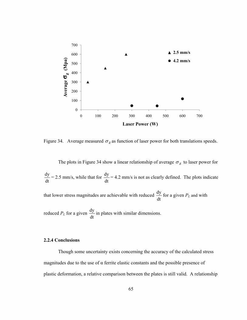
65
Figure 34. Average measured zσ as function of laser power for both translations speeds.
The plots in Figure 34 show a linear relationship of average zσ to laser power for
dtdy = 2.5 mm/s, while that for
dtdy = 4.2 mm/s is not as clearly defined. The plots indicate
that lower stress magnitudes are achievable with reduced dtdy for a given PL and with
reduced PL for a given dtdy in plates with similar dimensions.
2.2.4 Conclusions
Though some uncertainty exists concerning the accuracy of the calculated stress
magnitudes due to the use of α ferrite elastic constants and the possible presence of
plastic deformation, a relative comparison between the plates is still valid. A relationship
0
100
200
300
400
500
600
700
0 100 200 300 400 500 600 700
Aver
age σ z
(M
pa)
Laser Power (W)
4.2 mm/s
2.5 mm/s

66
between the measured values of the component of stress in the Z-direction and the input
parameters has been identified for plates of similar dimensions in which the average
value zσ within the samples was linearly proportional to input laser power at
dtdy = 2.5 mm/s, while those plates produced at
dtdy = 4.2 mm/s exhibit a non-linear
relationship that still shows lower stress magnitudes obtainable with lower laser powers.
The measured values of zσ in Sample 1 indicate that a change in geometry may
significantly impact the stress fields. However, further measurement of samples with
different geometries is needed to fully quantify this effect.
Though more data, i.e. a greater sample population produced with more
combinations of PL and dtdy , would be needed to generate a process map for optimization
of the LENSTM process toward minimization of residual stress. The experimentation
presented here, specifically the plots in Figure 34, suggest that the magnitudes of the
stress fields in simple geometric LENSTM parts may be reduced through a selection of
lower values of PL and dtdy . This finding may be beneficial to industry applications of
this process.

67
2.3 Simulation
2.3.1 Modeling with SYSWELD®
2.3.1.1 Introduction
The same 3-D model used by Wang et al. [20] for predicting temperature fields
and phase distributions was used in this study to calculate the thermal histories of the
deposited AISI 410 plates under varying conditions of laser power and stage translation
speed. A more detailed description of the coupled model is provided in Sections 2.3.1.2
and 2.3.1.3., while the constitutive model available in SYSWELD®, for calculating
residual stress is presented in detail in Section 2.3.1.4. The implementation of this model
and its comparison to the experimental diffraction measurements has been previously
published [30].
2.3.1.2 Theoretical Thermodynamic Model
In order to calculate the heat transfer to and from the plate during the LENSTM
deposition, a 3-D mathematical model developed by Wang et al. [20] was adopted, for
which the governing equation is:
( ) 0ALTkftTcf ij
jiij
iiiip
ii =∑+⎟
⎟⎠
⎞⎜⎜⎝
⎛∇⎟⎟⎠
⎞⎜⎜⎝
⎛∑∇−
∂∂
⎟⎟⎠
⎞⎜⎜⎝
⎛∑
<ρ
The heat source, simulating the laser, was modeled with the same Gaussian-
conical-distribution used by Wang et al. [20] and is described by the equation:
(6)

68
( )( ) ⎟⎟
⎟⎟⎟⎟
⎠
⎞
⎜⎜⎜⎜⎜⎜
⎝
⎛
⎥⎦
⎤⎢⎣
⎡−
−−
+
+−= 2
eei
eie
22
or
zzzzrr
r
yxQzyxQ exp,,
An ambient temperature was used as the initial condition throughout the domain before
the start of deposition, while the boundary conditions are described by:
Lower surface of substrate: ( ) oT0zyxT ==,,
Sides of plate: ( ) ( ) ( ) ΩΩΩΩ −−+−=⋅∇ r4
a4
a QTTTThnTk εσr
In Equation 9, the RHS represents the net heat flux into the deposited material. The first
term on the LHS represents the heat lost to convection, while second is the radiation heat
loss and the third is the energy input from the laser.
2.3.1.3 Phase Precipitation Model
The deposited material was considered to be multi-phased with thermal properties
that were weighted according to a linear mixture rule. The weighting of the mechanical
properties is discussed in Section 2.3.1.4. Volume fractions of phases evolved with
changing temperature according to a semi-empirical Koïstinen-Marbürger model in
which the phases austenite, ferrite, martensite, and tempered martensite were included.
As explained further in the next section, the substrate and deposited material were
initially modeled as ferritic before being austenized by the heat source, after which the
phase fraction of martensite precipitated after each thermal cycle is given by Equation 10
[31]
(7)
(8)
(9)

69
( ) ( ) ( )( )[ ] ooii MisAAM fTMk01ffTf +−−−+= exp. for Ti ≤ Ms
while that of retained austenite after each cycle is given by Equation (11)
( ) ( )( )isAA TMkfTf oi −−= exp for Ti ≤ Ms
Equations (10) and (11) are applied for all thermal cycles, i.e. every point in the
solution domain for each pass of the heat source. Since ferrite was only considered for
the initial metallurgical condition, the final state included only retained austenite,
martensite, and tempered martensite.
2.3.1.4 Theoretical Thermo-Metallurgical-Mechanical Model
The temperature and metallurgically-dependent mechanical features of the
LENSTM process are calculated in SYSWELD® with use of a phenomenologically-based
constitutive equation of state model developed by LeBlond [32] to describe the
temperature-dependent strain and stress fields that result in processes involving
thermally-driven phase transformation. This model partitions the total macroscopic strain
field according to Equation 12
TRIPThmPETotal EEEEE +++=
The first three terms on the RHS of Equation 12 describe macroscopic strain fields, while
the components of ETRIP are defined as micro-strains.
The elastic strains were considered to be isotropic with separate temperature
dependent elastic moduli for each phase present, while simple isotropic strain hardening
is chosen to describe the plastic zone. The overall yield strength of the material is
(10)
(11)
(12)

70
determined by a temperature-dependent, nonlinear rule of mixtures shown here as
Equation (13)
( ) ( )[ ] ( ) ( ) ( )TfFTfF1T jyj
iyjy σσσ +−=
The thermo-metallurgical strain is that due to the thermally-activated expansion
and contraction of each phase and the volumetric change resulting from phase
transformation as described in Equation 14
( ) ( )∑=
i
Thmii
Thmtotal TEffTE ,
Transformation-induced-plasticity is microscopic plastic strain resulting from the
macroscopic volumetric change included in EThm. In the case of the LENS TM material,
X20Cr13, the initial ferritic material is melted upon exposure to the heat source so that
the TRIP present in the final strain state is related only to austenite/martensite
transformations. In the case of such a two phase material, the TRIP occurs in the weaker
phase, i.e. austenite for X20Cr13. According to the LeBlond plasticity model [31,32,33],
TRIP will contribute to the overall plastic strain if the proper yield conditions are met, i.e.
if the equivalent stress (σeq = ijijSS23 ) is greater than or equal to the combined yield
strength defined in Equation 23, then an homogenous classical plastic strain occurs in
both phases. However, if σeq < σy, then the total plastic strain tensor receives both a
classic macroscopic contribution and one due to TRIP as in Equations 15 and 16.
TRIPCPP EEE +=
( ) M
y
eqijMA
y
ThmMATRIP
ij fhSfE2
23E ⎟
⎟⎠
⎞⎜⎜⎝
⎛⎟⎟
⎠
⎞
⎜⎜
⎝
⎛ Δ−= →
σσ
σln
(13)
(14)
(15)
(16)

71
2.3.1.5 Finite Element Model Development
The same 3-D finite element model presented by Wang et al. [20] was used to
approximate the experimental build conditions. The geometry consisted of a 5 mm x
1 mm x 10 mm plate, composed of 10 deposited layers 0.5 mm x 1 mm x 10 mm each,
and a 1mm x 4 mm x 10 mm substrate. The computational domain along with the
applied mesh is shown in Figure 35 below.
Figure 35. Computational domain used for LENSTM thin plate thermal analysis.
2.3.1.6 Finite Element Model Implementation
2.3.1.6.1 Thermal Calculations
For each case modeled, an initial temperature of 20 °C was applied over the whole
domain, while the bottom surface of the substrate was constrained to remain at 20 °C
Unit (mm)
Number of elements: 48252
Number of nodes: 37944
101
Element: 0.1 mm x 0.1 mm x 0.2 mm
1
5
X Y
Z
4

72
throughout the process. The convective heat transfer coefficient was specified as
h = 100 W/m2°C and the emissivity as ε = 0.62. A SYSWELD® subroutine was used to
model the Gaussian-distributed heat input as a moving heat source with a user-specified
velocity of 2.5, 4.2, and 8.5 mm/s. The initial beam radius, re, used in Equation 7 was set
to 0.5mm. Since most manufacturing applications of LENS TM control the applied laser
power through a thermal imaging feedback system similar to that presented by
Hofmeister et al. [8] to maintain near constant molten pool dimensions throughout the
build, a sequence of input energy densities, Qo, was established here for each value of
dtdy studied that would produce the same effect in the modeling. The calculated results at
some dtdy were compared to the measured stress values collected by neutron diffraction
for cases in which the average value of Qo used for all ten layers was close to the constant
applied laser power used to build the sample plate. These sequences are shown in Figure
36 below.
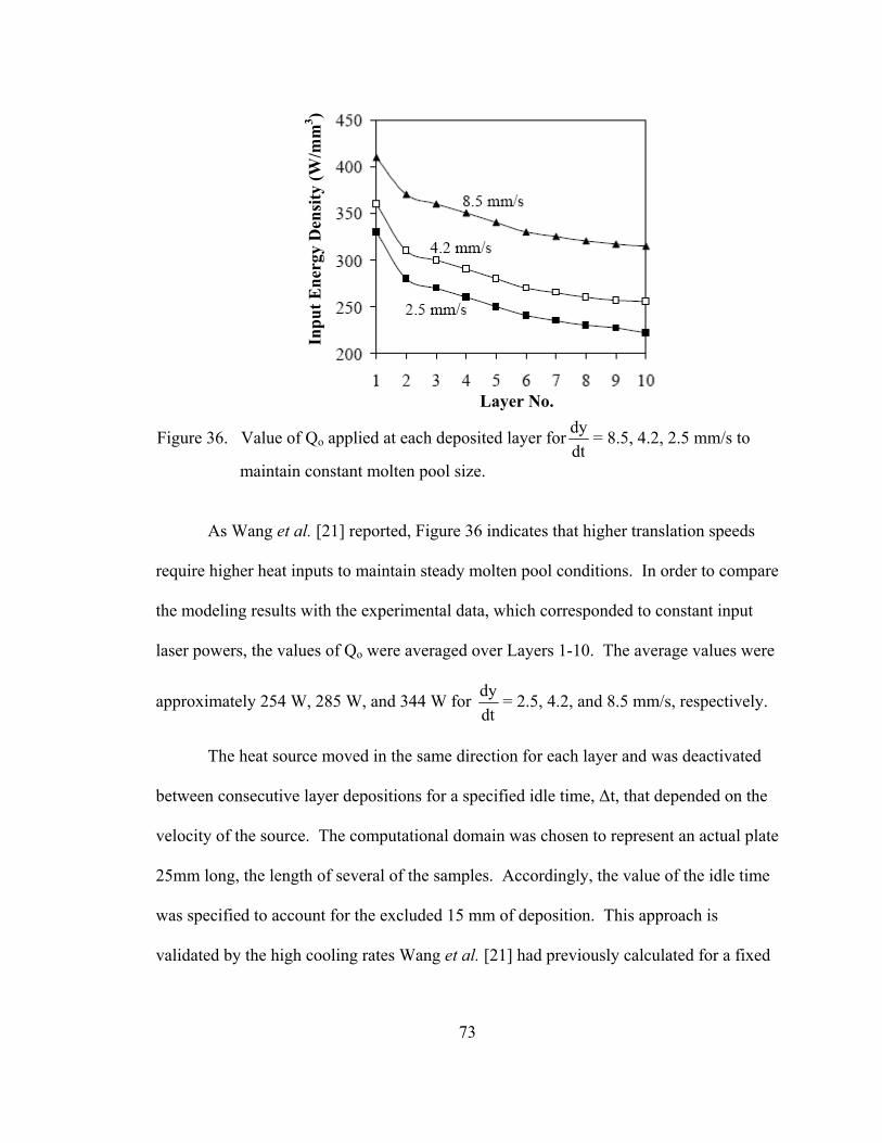
73
Figure 36. Value of Qo applied at each deposited layer fordtdy = 8.5, 4.2, 2.5 mm/s to
maintain constant molten pool size. As Wang et al. [21] reported, Figure 36 indicates that higher translation speeds
require higher heat inputs to maintain steady molten pool conditions. In order to compare
the modeling results with the experimental data, which corresponded to constant input
laser powers, the values of Qo were averaged over Layers 1-10. The average values were
approximately 254 W, 285 W, and 344 W for dtdy = 2.5, 4.2, and 8.5 mm/s, respectively.
The heat source moved in the same direction for each layer and was deactivated
between consecutive layer depositions for a specified idle time, Δt, that depended on the
velocity of the source. The computational domain was chosen to represent an actual plate
25mm long, the length of several of the samples. Accordingly, the value of the idle time
was specified to account for the excluded 15 mm of deposition. This approach is
validated by the high cooling rates Wang et al. [21] had previously calculated for a fixed
Inpu
t Ene
rgy
Den
sity
(W/m
m3 )
Layer No.

74
location, shown here as Figure 19 and those measured by Wang et al. [20] that are shown
in Figure 13, which revealed that the heating effects were very much localized.
The properties of the stainless steel alloy X20Cr13, which are provided in the
SYSWELD® material database, were applied to both the substrate and deposited material
since the chemical composition of this steel, shown in Table 3, is very similar to that of
AISI 410.
Table 3. Comparison of chemical compositions for AISI 410 and X20Cr13 stainless
steels.
Material Chemical Composition
AISI 410 C=0.15%, 11.5.%≤Cr≤13.0%, Mn=1.0%, Si=1.0%, S=0.03%, P=0.04%
X20Cr13 0.16%≤C≤0.25%, 12.0%≤Cr≤14.0%, Mn≤1.5%, Si≤1.0%, S≤0.03%, P≤0.04%
2.3.1.6.2 Coupled Thermo-Mechanical Calculations
The calculation procedure in SYSWELD®, shown here in Figure 37, involves a
strong coupling between thermal and metallurgical processes, where temperature and
phase proportions are solved simultaneously through Equations 6, 10 and 11.

75
Figure 37. Calculation scheme for thermal, metallurgical, and mechanical analyses in SYSWELD®.
A weak coupling relation is then employed for the mechanical calculations whereby the
temperature and metallurgical results are used as input for the model in Section 2.3.1.4.
2.3.1.7 Residual Stress Calculations
To provide comparison with the experimental results, the calculated Z-component
of stress, zσ , is analyzed. The 3-D distributions of the calculated stress values for
dtdy = 2.5, 4.2, and 8.5 mm/s are shown in Figure 38 for all ten layers.
σ, E
Mechanical
Thermal Boundary Conditions Initial Conditions Loads
Mechanical Boundary Condition
Thermal
Metallurgical
T
Lij fi

76
(a)
(b)
Figure 38. Distributions of zσ (MPa) in completed 10-layer plates for dtdy = a) 2.5
mm/s, b) 4.2 mm/s, c) 8.5 mm/s.
L10
L9
L8
L7
L6
L5
L4
L3
L2
L1
L10
L9
L8
L7
L6
L5
L4
L3
L2
L1
(MPa)
(MPa)

77
(c)
Figure 38 (Continued). The contours on Figure 38 appear highly pixilated since an average value is calculated for
each element and no smoothing was applied. However, the results clearly show a
congregation of tensile stresses at the outer surfaces of the plates and compressive values
near the plate centers. Additionally, the top layers, which are close to the free end, show
very small or zero values of residual stress. The calculated results compare well in a
qualitative manner with the measured distributions shown in Section 2.2.3 and those
collected by Rangaswamy, et al. [11].
Though little experimental data was available for comparison, the other principal
stress components yσ and xσ were also included in the calculations for the three values
ofdtdy . Figure 39 compares the calculated distributions of zσ and yσ for Layers 1, 3, 5,
7, and 9 in the direction of stage travel for at all three translation speeds.
L10
L9
L8
L7
L6
L5
L4
L3
L2
L1
(MPa)

78
(a)
Figure 39. zσ and yσ along width of plate at all dtdy in Layers a) 1, b) 3, c) 5, d) 7 and
e) 9.
2.5 mm/s 4.2 mm/s 8.5 mm/s
-200
-150
-100
-50
0
50
100
150
200
250
0 2 4 6 8 10
Z-co
mpo
nent
Res
idua
l Str
ess (
Mpa
)
Distance along travel direction(mm)
-250
-200
-150
-100
-50
0
50
100
150
0 2 4 6 8 10
Y-c
ompo
nent
Res
idua
l Str
ess (
Mpa
)
Distance along travel direction(mm)

79
(b)
Figure 39 (Continued).
2.5 mm/s 4.2 mm/s 8.5 mm/s
-200
-150
-100
-50
0
50
100
150
200
250
0 2 4 6 8 10
Z-co
mpo
nent
Res
idua
l Str
ess (
Mpa
)
Distance along travel direction(mm)
-150
-100
-50
0
50
100
150
200
0 2 4 6 8 10
Y-c
ompo
nent
Res
idua
l Str
ess (
Mpa
)
Distance along travel direction(mm)

80
(c)
Figure 39 (Continued).
2.5 mm/s 4.2 mm/s 8.5 mm/s
-150
-100
-50
0
50
100
150
200
0 2 4 6 8 10
Z-co
mpo
nent
Res
idua
l Str
ess (
Mpa
)
Distance along travel direction(mm)
-150
-100
-50
0
50
100
150
200
250
0 2 4 6 8 10
Y-co
mpo
nent
Res
idua
l Str
ess (
Mpa
)
Distance along travel direction(mm)

81
(d)
Figure 39 (Continued).
2.5 mm/s 4.2 mm/s 8.5 mm/s
-150
-100
-50
0
50
100
150
200
250
0 2 4 6 8 10
Y-c
ompo
nent
Res
idua
l Str
ess (
Mpa
)
Distance along travel direction(mm)
-150
-100
-50
0
50
100
150
0 2 4 6 8 10
Z-co
mpo
nent
Res
idua
l Str
ess (
Mpa
)
Distance along travel direction(mm)
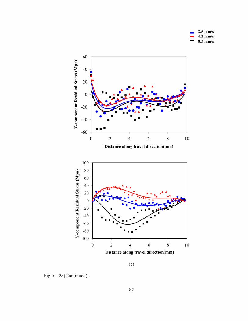
82
(e)
Figure 39 (Continued).
2.5 mm/s 4.2 mm/s 8.5 mm/s
-60
-40
-20
0
20
40
60
0 2 4 6 8 10
Z-co
mpo
nent
Res
idua
l Str
ess (
Mpa
)
Distance along travel direction(mm)
-100
-80
-60
-40
-20
0
20
40
60
80
100
0 2 4 6 8 10
Y-c
ompo
nent
Res
idua
l Str
ess (
Mpa
)
Distance along travel direction(mm)
83
The solid lines in Figure 39 are the fitted curves for the numerical data points.
The plots show that zσ and yσ are similarly compressive at the two lower speeds, but
that yσ becomes tensile at dtdy = 8.5 mm/s in all layers except Layer 9, where the tensile
values are instead taken on by zσ and yσ . Wang et al. [30] theorized that the tensile
nature of yσ at dtdy = 8.5 mm/s is due to the higher cooling rates predicted at higher
speeds, as shown in the parametric study in Reference [21]. These rapid cooling rates
may prevent relaxation of the internal stresses after the initial deformation.
Interestingly, the results show magnitudes and distributions of yσ similar to those
measured for Sample 4 in Section 2.2.3. However, contrary to the measured data in
which the values of yσ were significantly less than those of zσ , the computed results
show the two components as being approximately the same size, though no precise
comparison can be made, since the combination of laser power and speed used to build
Sample 4 was not modeled.
The calculated distributions of zσ and yσ along the vertical plate centerline for
all values of dtdy are shown in Figure 40. The plots in Figure 40 pertain to Layers 3-10
of the computational domain, which closely approximates the region of the sample plates
in which data was collection. The computed zσ profile is quite similar in a qualitative
sense to the measured data, whereby increasing compressivity results with increased

84
depth from the top surface. As in the horizontal direction, yσ becomes tensile at dtdy =
8.5mm/s.
(a)
(b)
Figure 40. Distribution of a) zσ and b) yσ along vertical center line for alldtdy .
A direct comparison between the experimental and modeling results is difficult
due to the constant versus variable heat inputs used for the actual builds and simulated
-140-120-100
-80-60-40-20
020
0 1 2 3 4 5
-200-150-100-50
050
100150200250300
0 1 2 3 4 5
Y-C
ompo
nent
Res
idua
l Str
ess (
MPa
) Z
-Com
pone
nt R
esid
ual S
tres
s (M
Pa)
Distance from free end (mm)
Distance from free end
2.5 mm/s4.2 mm/s8.5 mm/s
2.5 mm/s4.2 mm/s8.5 mm/s

85
builds, respectively. An additional complication arises from the reduced dimensions of
the computational domain in relation to the sample plate geometries. Accordingly, a
qualitative evaluation is made amongst the experimental and modeling results with same
dtdy . To account for the geometrical differences, the experimental and calculated
distributions of zσ are compared in a region from the top layer to a depth of 5mm along
the vertical plate centerline. For the horizontal distributions, values of zσ are examined
in a region extending 5mm in the Y-direction from either side of the vertical centerline.
The modeling results were taken along Layer 5, which corresponded to the horizontal
centerline of the computational domain. The experimental and modeling results for
dtdy = 2.5mm/s are shown in Figure 41.

86
(a)
(b)
Figure 41. Experimental and computational yσ distributions for dtdy =2.5 mm/s along a)
vertical plate axis and b) along width from vertical centerline.
-700
-600
-500
-400
-300
-200
-100
0
100
200
-6 -4 -2 0 2 4 6
Distance from free end (mm)
Z-C
ompo
nent
Res
idua
l Str
ess (
MPa
) Z
-Com
pone
nt R
esid
ual S
tres
s (M
Pa)
Distance from center along Y-axis (mm)
300W (#1)
450W (#6)
600W (#4)
Modeling
300W (#2)
300W (#1)
450W (#6)
600W (#4)
Modeling
300W (#2)

87
The plot in Figure 41(a) shows that the modeling results, which correspond to an average
energy input density of 254 W/mm3, follow the same general trend of increasingly
compressive stress with the distance from the free end as the measured distributions. The
calculated results presented in Figure 41(b) are closest to those measured values
associated with an input laser power of 300 W.
A comparison between the experimental and computational distributions of zσ at
a translation speed of 4.2 mm/s is shown in Figure 42. As in Figure 41, the plots in
Figure 42 show that the calculated values lie within the range of the experimental data,
for which the measured values of zσ were close for all samples at these locations. Since
no diffraction measurements were performed on plates produced with dtdy = 8.5 mm/s, no
experimental comparison could be performed for with those calculations.

88
(a)
(b)
Figure 42. Experimental and computational zσ distributions for dtdy = 4.2 mm/s along
a) vertical plate axis and b) along width from vertical centerline.
-400
-300
-200
-100
0
100
200
300
400
-6 -4 -2 0 2 4 6
Distance from free end (mm)
Z-C
ompo
nent
Res
idua
l Str
ess (
MPa
)
Distance from center along Y-axis (mm)
Z-C
ompo
nent
Res
idua
l Str
ess (
MPa
)
300W (#3)
600W (#5)
450W (#7)
Modeling
300W (#3)
600W (#5)
450W (#7)
Modeling

89
2.3.1.8 Conclusions
The comparison of the measured and modeled results in Figure 41 shows the
calculated distributions of zσ , with average heat inputs of Qo = 254 W/mm3, aligning
most closely with the sample plates built with 300 W laser power, indicating that the FE
model is able to capture this parametric relation for a given speed. At dtdy = 4.2 mm/s,
the relationship between zσ and input laser power is not as clear in the regions
examined. However, the calculated results reside within the limits set by the measured
data.
The comparisons presented in Figures 41 and 42 for zσ show that the
calculations made with SYSWELD® can provide reasonable approximations of the
measured data for different values ofdtdy . Additionally, the numerical values of yσ were
similar to those observed in one of the sample plates. However, additional experimental
samples produced under more combinations of input parameters and further simulations
would be needed to ascertain whether the model is truly able to predict residual stresses
for a wide range of values fordtdy and PL.
2.3.2 Modeling with ABAQUS®
2.3.2.1 Introduction
The previously presented modeling results produced using SYSWELD® have
shown that this FE package is capable of giving reasonably accurate predictions of

90
residual stresses generated during the LENS™ process in multi-phase steel alloy.
However, the LeBlond constitutive model used by SYSWELD® to predict the stress state
is an equation of state model based in part on external observations and excludes several
important physically-grounded aspects of deformation. Though this type of model is
reasonably accurate within the elastic limit, it cannot properly account for the dissipative
effects that take place in inelastic materials. An internal state variable (ISV) type model,
which is characterized by the use of rate equations to track the evolution of unobservable,
macroscopic state variables, is better suited for describing irreversible processes and is a
more appropriate choice for modeling the complexities of LENS™. One such model was
developed by D. Bammann at Sandia National Laboratory and, in conjunction with M.
Chiesa and G. Johnson [34] and was incorporated into a computational formulation
widely known as the BCJ plasticity code. This code has been used to model complex
thermo-mechanical processes, such as welding and heat treating for single-phase
materials by Dike et al [35] and Bammann et al. [36]. The theoretical model was
expanded by Bammann et al. [37] to describe a two-phase material that undergoes
austenite/martensite transformation through a kinetic model developed by Oddy et al.
[38].
The two-phase model can be implemented in ABAQUS® via the BCJ code as a
user defined material subroutine or UMAT. Though such a subroutine has been
developed that incorporates a two phase version of the BCJ code, to date no calculations
have been performed as the material input parameters needed for the model are not
currently available for either X20Cr13 or AISI 410 stainless steels in the literature.
However, when these parameters are recorded or when experimental data is measured for

91
LENS™ deposition of some material for which parameters already exist, the model can
be implemented through ABAQUS® and compared to measured values.
A prerequisite to thermo-mechanical LENSTM modeling in ABAQUS® is the
ability to accurately predict the thermal conditions generated during the deposition that
would subsequently drive microstructural transformations and thermally-initiated
deformation. Accordingly, ABAQUS® 6.7 was used to model the thermal characteristics
of the LENS™ deposition of a 10-layer thin plate to validate that this FEA package is
capable of accurately predicting the thermal histories. The calculated temperature
distributions were then compared to experimentally measured data from Hofmeister et al.
[6] and also to modeling results produced with SYSWELD® by Wang et al. [21].
Additionally, simulations for 10-layer thin plate deposition were made with the
ABAQUS® for different values ofdtdy . The resulting molten pool sizes were measured
and compared to those found using SYSWELD® by Wang et al. [30], which were
validated experimentally in that study.
2.3.2.2 Theoretical Thermal Model
The mathematical thermal model used for the ABAQUS® calculations are
essentially the same as those in the SYSWELD® model except for simplification, the
material is modeled as single-phased, where each thermal property (ρ, k, cp, and L) is
calculated as a temperature-dependent average of those for the included phases.
Accordingly, phase transformation is not accounted for in the thermal calculations, i.e. no

92
temperature-dependent weighting scheme is used. The resultant governing equation is
presented here as Equation 27.
( ) ( ) ( )( ) ( ) 0TTTT
tTLTTk
tTTcT
sl
sp =⎟⎟
⎠
⎞⎜⎜⎝
⎛−−
∂∂
+∇∇−∂∂ρ
The applied boundary conditions thermal loads are the same as those given as
Equations 7-9 in Section 2.3.1.2.
2.3.2.3 Finite Element Model
The computational domain used for the ABAQUS® modeling was given the same
dimensions previously presented in Section 2.3.1.4. The mesh was composed of linear,
8-noded DC3D8 heat transfer brick elements. The details of the mesh geometry are
shown in Figure 43.
(27)

93
Figure 43. Computational mesh for 10-layer LENS™ thin plate in ABAQUS®.
The mesh created in ABAQUS® is not as fine as that used for the SYSWELD®
calculations. The appropriate degree of refinement was determined by first modeling the
thermal process with a coarse mesh of 1197 nodes and 1184 elements to obtain a
temperature field. The mesh refinement was then doubled and a subsequent simulation
performed. The new temperature field was compared to the previous results to determine
whether the solution was mesh-dependent. This procedure was repeated until the
deviation in field values between consecutive meshes was acceptably small, indicating
mesh-independency.
No. Nodes: 16167 No. Elements: 13300 Element Type: DC3D8 10mm
1mm
5mm
X Y
Z
4mm
1mm
Element: 0.2mm x 0.167mm x 0.167mm
94
2.3.2.4 Model Implementation
The heat transfer analysis performed in ABAQUS® is an un-coupled thermal
calculation in which the temperature field is solved for conditions of solid-body
conduction, basic convection and radiation heat transfer, as well as latent heat generation.
The thermal loading of the plate is modeled as a transient temperature analysis with a
semi-automatic time incrementation scheme, in which an upper limit is placed on the
length of the time increments by a user-specified maximum temperature change [39].
The deposition process is modeled with the same element activation function used
by Neela and De[16] and Deus and Mazumder[17], which is defined as the
MODEL_CHANGE feature in ABAQUS® 6.7. For these calculations, each layer was
composed of ten 0.5 x 1.0 x 1.0 mm3 element sets, containing 60 elements. A new
element set was activated at the beginning of a user-defined time step, entering the active
domain with an artificially low value of thermal conductivity that was ramped up to the
specified values of X20Cr13 to ensure a smooth transition [39]. Upon entering the active
domain, the new element set was loaded with a stationary heat source, Qr from Equation
7, which was applied for the length of the time step. A total of 100 time steps was used
to model the deposition of the plate, where every time step corresponded to the activation
and heating of an element set. During each time step the coordinates of the heat source
were set to coincide with the center of the newly activated element set. For simplicity,
this approach was used to approximate the moving laser instead of using a user-defined
subroutine. The length of the time step, i.e. the element set activation rate, depended on
the translation speed being examined as seen in Equation 28.

95
dtdyL
dt e=
Additionally, the same idle times described in Section 2.3.1.5.1 are again used between
consecutive layers to account for geometric differences between the computational
domain and a 25 mm long plate.
2.3.2.5 Thermal Calculations
Hofmeister et al. [6] produced a thin plate of AISI 316 stainless steel was
deposited by LENSTM using PL=275 W and dtdy =7.62 mm/s. During the deposition of
one of the layers, thermal imaging was used to capture the temperature distribution with
distance from the center of the molten pool in the direction opposite to heat source travel
when the laser was located at the mid-width of the deposited plate. The plotted
distribution is shown here as Figure 3 in Section 1.2.1. These measured values were
compared by Wang et al. [21] to a calculated temperature distribution for a simulated
plate using SYSWELD® under the same processing conditions. The modeling results
were shown to closely approximate the actual temperature field, and this comparison was
presented as a validation of the FE model [21].
Similarly, this deposition was modeled in ABAQUS® to gauge the accuracy of
the model presented in Section 2.3.2.3. Applying single phase thermal properties of AISI
316 to the elements and the same load and boundary conditions specified by Wang et al.
[21], the temperature field was calculated with the heat source located at the mid-width of
the domain for the 10th deposited layer. The resulting temperature distribution was
(28)

96
plotted as a function of distance from the center of the molten pool in the direction
opposite to deposition and compared to both the measured values and those found with
SYSWELD®. This comparison is shown here as Figure 44. The plots in Figure 44 show
the calculations made with ABAQUS® are in good agreement with the experimental data
as well as the SYSWELD® predictions, though in both instances, the modeling under-
predicts the temperature in the region from 1 mm-4mm from the molten pool center,
which may indicate that the specified convective and radiation boundary conditions need
to be adjusted.
Figure 44. Comparison of numerical and experimental temperatures measured from center of molten pool in top layer of LENS™ AISI 316.
800
1000
1200
1400
1600
1800
0 1 2 3 4
Modeling – ABAQUS®Modeling – SYSWELD® [21]Experimental [6]
Distance from center of molten pool in Y-direction (mm)
Tem
pera
ture
(°C
)

97
In order to further validate the ability of the model presented Section 2.3.2.3 to
accurately predict thermal LENSTM conditions, calculations were performed for the
LENSTM deposition of a ten layer plate of X20Cr13 stainless steel at values of dtdy = 4.2
mm/s, and 8.5 mm/s using the same thermal boundary conditions and sequences of Qo
shown in Section 2.3.1.6.1, Figure 36. The same idle time between consecutive layer
depositions was also imposed. The resulting molten pool dimensions in each layer were
then compared to the corresponding SYSWELD® predictions, which were
experimentally verified by Wang et al. [20].
In the calculations X20Cr13 was considered as a two-phase material composed of
martensite and austenite, the thermal properties of which were obtained for each phase
from the SYSWELD® material database. Each thermal property (ρ, k, cp, and L) was
calculated as a temperature-dependent average of those given for the two phases over a
range of 20°C to 1530°C, i.e. from room temperature to the liquidus of X20Cr13.
2.3.2.6 Results and Comparison with SYSWELD®
The resulting molten pool widths (Y-direction) are shown in Figure 45 for each
layer when the heat source is located at the plate center. The corresponding
SYSWELD® predictions are also shown for comparison. The shapes of the pools appear
quite different due to the differing techniques used for simulating the material deposition.
Specifically, the SYSYWELD® “dummy element” operation activates entire layers,
while the MODEL_CHANGE operation in ABAQUS® allows user-defined element sets

98
to be activated individually during the deposition of a layer. The maximum pool size
observed at the center of the plates for all ten layers is displayed in Figure 45.
(a)
Figure 45. Comparison of molten pool sizes calculated with ABAQUS® and
SYSWELD® for dtdy = a) 4.2 mm/s and b) 8.5 mm/s.
10 9 8 7 6 5 4 3 2 1
1.7 mm 1.6 mm

99
(b)
Figure 45 (Continued).
The ABAQUS® results show more growth of the molten pool from layer to layer, which
may be due to the exclusion of phase transformation from these calculations. However,
despite the variations in approach, reasonable agreement is found between the two
models. Accordingly, Figures 45 shows that essentially the same thermal histories can be
generated in the computational domain when the same process parameters are applied.
10 9 8 7 6 5 4 3 2 1
1.9 mm 1.9 mm
100
CHAPTER 3
CONCLUSION
The LENS™ process is a laser deposition technique that is able to economically
repair and fabricate metallic components of various geometries, but the relation between
final form mechanical properties and the process parameters are not well understood. A
thorough review of the published literature on parametric research of LENS™ has been
performed here and the major findings reported. A study was then presented in which the
finite element method was used to model the thermal, metallurgical, and mechanic
features in the deposition of a single-pass, stainless steel plate built with different values
of the input parameters, stage translation speed and laser power. Calculations were first
performed with the finite element software, SYSWELD®. The residual stress state
resulting from each simulation was compared to measured values collected via the
neutron diffraction method. The modeling was found to provide reasonably accurate
predictions. Further thermal calculations were performed using the finite element
software ABAQUS® 6.7 to predict temperature fields and molten pool sizes in the same
stainless steel plate with the same process parameter combinations previously used. The
calculated temperature profiles closely matched those found with SYSWELD®, which
had already been validated through experimental comparison. Accordingly, the ability of
ABAQUS® to provide accurate thermal output was qualified, so that a two-phase version

101
of the BCJ internal state variable plasticity model could be applied to modeling residual
stresses in LENS™ and implemented via an ABAQUS® user-defined subroutine.
Future efforts to model the effects of process parameters on resulting LENSTM
deposits of multi-phase ferrous alloys may make use of the model presented in Section
2.3.2 and the two-phase ISV model developed by Bammann et al. [37] in a coupled
thermo-metallurgical-mechanical analysis if mechanical testing is performed to obtain the
appropriate material properties of X20Cr13 stainless steel or AISI 410 stainless steel as
inputs for the ABAQUS® user-defined material subroutine. These material properties
and their significance in terms of material behavior have been described by Bammann et
al. [36]. Residual stress magnitudes and distributions obtained using this model may then
be compared to the experimental measurements and the SYSWELD® predictions
presented in section 2.3.1 to determine if the ISV is truly capable of more accurately
representing the thermo-metallurgical-mechanical characteristics of the LENSTM process.

102
BIBLIOGRAPHY
[1] Vilar, R. J. Laser Cladding. Laser Appl. Vol 11. No 2. 1999. Pp. 64-79. [2] Atwood, C., Griffith, M., Harwell, D., Reckaway, D., Ensz, M., Keicher, D.,
Schlienger, M., Romero, M., Oliver, M., Jeanette, F., Smugeresky, J. Laser Spray Fabrication for Net-Shape Rapid Product Realization LDRD. Sandia Report.1999.
[3] Sandia National Laboratories website.
(http://www.sandia.gov/mst/technologies/net-shaping.html). [4] Griffith, M., Ensz, M., Puskar, J., Robino, C., Brooks, J., Philliber, J.,
Smurgeresky, J., Hofmeister, W. Understanding the microstructures and properties of components fabricated by laser engineered net shaping(LENS). Mat. Res. Soc. Symp. Proc. Vol 625. Warrendale, PA. 2000. Pp. 9-21.
[5] Keicher, D. Jellison, J., Schanwald, L., Romero, J. Towards a reliable laser spray
powder deposition system through process characterization. 27th Int. Tech. Conf. Soc. Adv. Mat. Pro. Eng. Alburquerque, NM. 1995. Pp. 1009-1018.
[6] Hofmeister, W., Wert, M., Smurgeresky, J., Philliber, J., Griffith M., Ensz, M.
Investigating solidification with the laser-engineering net shaping (LENS™) process. JOM-e. http://www.tms.org/pubs/journals/JOM/9907/Hofmeister/Hofmeister-9907.html. Accessed Aug 2007.
[7] Hofmeister, W., Griffith, M., Ensz, M., Smurgeresky, J. Solidification in direct
metal deposition by LENS processing. JOM. Vol.53. No 9. 2001. Pp. 30-34. [8] Hofmeister, W., MacCalum, D., Knorovsky, G. Video monitoring and control of
the LENS process. American Welding Society 9th International Conference of Computer Technology in Welding. Detroit, MI. 1998. Pp. 187–196.
[9] Smugeresky, J., Keicher, D., Romero, J., Griffith, M., Harwell, L. Laser
engineered net shaping (LENSTM) process: optimization of surface finish and microstructural properties Proc. of the World Congress on Powder Metallurgy and Particulate Materials. Princeton, NJ. 1997. Part 21.

103
[10] Kahlen, F.-J., Kar, A. J. Tensile strengths for laser-fabricated parts and similarity parameters for rapid manufacturing. Manuf. Sci. Eng. Vol 123. No 1. 2001. Pp. 38-44.
[11] Rangaswamy, P., Holden, T., Rogge, R., Griffith, L. J. Residual stresses in
components formed by the laser-engineered net shaping (LENS®) process. Strain Analysis. Vol 38. No 6. 2003. Pp. 519-528. [12] Rangaswamy, P. Griffith, M., Prime, M., Holden, T., Rogge, R., Edwards, J.,
Sebring, R. Residual stresses in LENS® components using neutron diffraction and contour method.Mat. Sci. Eng. A. Vol 399. 2005. Pp. 72-83.
[13] Riqing, Y., Smugeresky, J., Zheng, B., Zhou, Y., Lavernia, E. Numerical modeling of the thermal behavior during the LENS® process. Mat. Sci. Eng. A. Vol 428. 2006. Pp. 47-53.
[14] Lindgren, L.-E. Finite element modeling and simulation of welding part :
increased complexity. Journal of Thermal Stresses. Vol 24. 2001. Pp. 195-231. [15] Wang, L., Felicelli, S. Analysis of thermal phenomena in LENS™ deposition.
Mater. Sci. Eng. A. Vol 435-436. 2006. Pp. 625-631. [16] Neela, V., De, A. Numerical modeling of LENS™ process using special
element features.2007 Abaqus India Regional Users’ Meeting. 2007. http://www.simulia.com.
[17] Deus, A., Mazumder, J. Two-dimensional thermo-mechanical finite element model for laser cladding. Proc. ICALEO. Duley, W., Shibata, K., Poprawe, R., eds. Orlando, FL. Laser Institute of America. 1996. Pp. B/174-B/183.
[18] Labudovic, M., Hu, D., Kovacevic, R. A three dimensional model for direct laser
metal powder deposition and rapid prototyping.J. Mat. Sci. Vol 38. 2003. Pp. 35-49. [19] Costa, L., Vilar, R., Reti, T., Deus, A. Rapid tooling by laser
deposition : process simulation using finite element analysis Act. Mat. Vol 53. 2005. Pp. 3987-3999.
[20] Wang, L., Felicelli, S., Craig, J. Thermal modeling and experimental validation in the LENSTM
process. 18th Solid Freeform Fabrication Symposium. Austin, TX. Aug 6-7, 2007. Pp 100-111. [21] Wang, L., Felicelli, S., Gooroochun, Y., Wang, P., Horstemeyer, M. Optimization
of the LENS® process for steady molten pool size.Mater. Sci. Eng. A. Vol 474. 2007. Pp. 148-156.

104
[22] Vasinonta, A., Beuth, J. Process maps for controlling residual stress and melt pool size in laser-based SFF process. Proc. 11th Solid Freeform Symposium. Austin, TX. Aug 7-9, 2000. Pp. 200-208.
[23] Allen, A., Hutchings, M., Windsor, C. Neutron diffraction methods for the study
of residual stress fields. Adv. Phys. Vol 34. 1985. Pp. 445-473. [24] Pratt, P., Felicelli, S., Wang, L., Hubbard, C. Residual stress measurements of
LENS AISI 410 thin plates via neutron diffraction Met. Mat. Trans. A. 2008. (Accepted)
[25] Winholtz, R. Analysis of Residual Stress by Diffraction using Neutron and Synchrotron Radiation. Fitzpatrick, M. and Lodini, A., eds. Taylor and Francis, NY. 2003. Pp. 60-77. [26] Behnken, V., Hauk, Z. Berechung der röntgenographischen elastizitätskonstanten
(REK) des vielkristalls aus den einkristalldaten für beliebige kristallsymmetrie. Z. Metallkd. Vol 77. 1985. Pp. 620-626.
[27] Dever, D. J. Temperature dependence of the elastic constants in α-iron single
crystals: relationship to spin order and diffusion anomalies.Appli. Phys. Vol 43. 1972. Pp. 3293-3301.
[28] Kröner, E. Berechung der elastischen konstanten des vielkristalls aus den
konstanten des einkristalls.Z. Phys. Vol 5. 1958. Pp. 504-518. [29] Smith, W. Stainless Steels in Structures and Properties of Engineering Alloys. 2nd
Edition. McGraw-Hill. NY. 1993. p 310. [30] Wang, L., Felicelli, S., Pratt, P. Residual stresses in LENS-deposited AISI 410
Stainless Steel Plates. Mat, Sci. Eng. A. Vol 496. 2008. P. 234-241. [31] SYSWELD 2005 Reference Manual, ESI Group, 2005. [32] LeBlond, J. A theoretical and numerical approach to the plastic behavior of steels
during phase transformations – I. derivation of general relations. J. Mech. Phys. Solids. Vol 34. No 4. 1986. Pp. 395-409.
[33] LeBlond, J. A theoretical and numerical approach to the plastic behavior of steels
during phase transformations – II. Study of classical plasticity for ideal-plastic phases. J. Mech. Phys. Solids. Vol 34. No 4. 1986. Pp. 411-432.

105
[34] Bammann, D., Chiesa, M., Horstemeyer, M., Weingarten, L. Failure in ductile materials using finite element method, in Structural Crashworthiness and Failure. Jones, N. and Weirzbicki, T., eds. Elsevier, Amsterdam. 1993. pp 1-54.
[35] Dike, J., Brooks, J., Bammann, D., Li, M. Finite element modeling of weld solidification cracking in 6061-T6 aluminum – applicability of strain-based failure criteria. Proceedings of the 2nd International Symposium on Thermal Stresses and Related Topics. Rochester, NY. 1997.
[36] Bammann, D., Prantil, V., Kumar, A., Lathrop, J., Mosher, D., Callabresi, M.,
Lusk, M., Krauss, G., Jou, H., Elliot, W., Ludtka, G., Dowling, W., Nikkel, D., Lowe, T., Shick, D. Development of a carburizing and quenching simulation tool: a material model for low carbon steels undergoing phase transformations. American Society of Metals 2nd International Conference on Quenching and Control of Distortion. Cleveland, OH. 1996. Pp. 367-375.
[37] Bammann, D., Prantil, V., Lathrop, J. A model of phase transformation plasticity,
in Modeling of Casting, Welding and Advanced Solidification Processes VII. Cross, M., and Campbell, J., eds. TMS. 1995. Pp. 275-284.
[38] Oddy, A., McDill, J., Karlsson, L. Microstructural predictions including arbitrary
thermal histories, reaustenization and carbon segregation effects. Canadian Metallurgical Quaterly. Vol 35. No 3. 1996. Pp. 137-146.
[39] ABAQUS® Analysis User’s Manual, Version 6.7. 2007. Simulia, Inc.