dynamic nonlinear soil-structure interaction
TRANSCRIPT
HAL Id: tel-00453297https://tel.archives-ouvertes.fr/tel-00453297
Submitted on 4 Feb 2010
HAL is a multi-disciplinary open accessarchive for the deposit and dissemination of sci-entific research documents, whether they are pub-lished or not. The documents may come fromteaching and research institutions in France orabroad, or from public or private research centers.
L’archive ouverte pluridisciplinaire HAL, estdestinée au dépôt et à la diffusion de documentsscientifiques de niveau recherche, publiés ou non,émanant des établissements d’enseignement et derecherche français ou étrangers, des laboratoirespublics ou privés.
Dynamic nonlinear soil-structure interactionEsteban Saez Robert
To cite this version:Esteban Saez Robert. Dynamic nonlinear soil-structure interaction. Other [cond-mat.other]. EcoleCentrale Paris, 2009. English. NNT : 2009ECAP0012. tel-00453297

ECOLE CENTRALE DES ARTS
ET MANUFACTURES
« ECOLE CENTRALE PARIS »
THESEpresentee par
Esteban Patricio SAEZ ROBERT
pour l’obtention du
GRADE DE DOCTEUR
Specialite : Modelisation numerique, Dynamique des Sols
Laboratoire d’accueil : Mecanique des Sols, Structures et Materiaux
SUJET: DYNAMIC NONLINEAR SOIL-STRUCTURE INTERACTION
Soutenue le: 20 mars 2009
devant un jury composee de:
M. BISCH Philippe President
Mme. MODARESSI Arezou Directrice de These
M. PAOLUCCI Roberto RapporteursM. PITILAKIS Kyriazis
Mme. FOERSTER Evelyne ExaminateursM. LOPEZ-CABALLERO Fernando
M. CLOUTEAU Didier Invite
2009-ECAP0012

Avant-propos
Cette these a ete realisee au laboratoire de Mecanique des Sols, Structures et Materiaux de l’EcoleCentrale de Paris. Elle a ete partiellement financee par une bourse CONICYT du Gouvernementchilien ainsi que partiellement par une bourse accordee par la Direction de la recherche du BRGM.
Je tiens ainsi a remercier tout d’abord ma directrice de these, Arezou MODARESSI, pour sonencadrement soigne, ses encouragements et ses conseils precieux dans l’orientation de mon travail. Jeremercie tout particulierement Fernando LOPEZ-CABALLERO, pour tout l’interet qu’il a porte surcette these et son aide tout au long de ce travail. Je remercie egalement Didier CLOUTEAU, qui parses conseils et sa disponibilite, a tres largement contribue a ma these. A Etienne BALMES, j’adresseaussi mes remerciement pour sa collaboration efficace.
Je voudrais aussi exprimer ma gratitude a Messieurs Roberto PAOLUCCI et Kyriasis PITILAKIS,qui m’on fait l’honneur d’accepter la lourde tache d’etre rapporteurs de ma these. Je remercie egale-ment M. Philippe BISCH et Mme. Evelyne FOERSTER qui ont aimablement accepte d’examinermon travail.
Enfin je tiens a associer a ces remerciements tous les membres du laboratoire MSSMAT, pour leuraide et les moments agreables que nous avons passes ensemble au cours des ces annees. Je penseparticulierement a Alex, Amelie, Anne-Sophie, Cristian, Denis, Elsa, Florent, Ghizlane, Hormoz,Isabelle, Jean-Louis, Madhia, Michael, Nadege, Pierre, Pauline, Quang Anh, Rachele, Regis, Reza,Sofia, Stephane, Tammam et autres qui ont contribue a faire de mon passage a l’ECP une excellenteexperience personnelle et scientifique.

Abstract
The dynamic interaction of the soil with a superstructure (DSSI) has been the subject of numerousinvestigations assuming elasticity of both, superstructure and soil foundation behavior. Nevertheless,the effect of DSSI may differ between elastic and inelastic systems. Thus, the current interactionmethodologies based on elastic response studies could not be directly applicable to structures ex-pected to behave inelastically during severe earthquakes. Additionally, the soil is known to exhibitinelastic behavior even for relatively weak to moderate ground motions. Consequently, ignoring thesecharacteristics in studying DSSI could lead to erroneous predictions of structural damage.
The main purpose of this work is to develop a general strategy to address the full DSSI problem inthe context of the seismic vulnerability analysis of structures. Thus, realistic Finite Elements modelsare constructed and applied in a practical way to deal with these issues. These models cover a largerange of soil conditions and structural typologies under several earthquake databases. Some modelingstrategies are introduced and validated in order to reduce the computational cost. Therefore, anequivalent 2D model is developed, implemented in GEFDyn and used in the large parametric studyconducted. Several indicators for both structural and soil responses are developed in order to synthesizetheir behavior under seismic loading. Additionally, a vulnerability assessment strategy is presented interms of measures of information provided by a ground motion selection.
According to the investigation conducted in this work, there is in general a reduction of seismicdemand or structural damage when non-linear DSSI phenomenon is included. This reduction canbe associated fundamentally to two phenomena: radiative damping and hysteretic damping due tonon-linear soil behavior. Both effects take place simultaneously during the dynamic load and it is ex-tremely difficult to separate the contribution of each part in reducing seismic demand. Indeed, effectivemotion transmitted to the superstructure does not correspond to the free field motion because of thegeometrical and inertial interactions as well as the local modification of soil behavior, specially dueto the supplementary confinement imposed by the superstructure’s weight. A series of strong-motionseverity measures, structural damage measures and energy dissipation indicators have been introducedand studied for this purpose. Nevertheless, results are erratic and consequently, generalization wasextremely difficult.
Despite these difficulties, the results illustrate the importance of accounting for the inelastic soilbehavior. The major part of the studied cases show beneficial effects such as the decrease of themaximum seismic structural demand. However, the non-linear DSSI could increase or decrease the ex-pected structural damage depending on the type of the structure, the input motion, and the dynamicsoil properties. Furthermore, there is an economic justification to take into account the modificationeffects due to inelastic soil behavior.
Keywords: dynamic soil-structure interaction, non-linear behavior, finite elements, coupled for-mulation, structural damage, ductility demand, seismic vulnerability

Resume
L’interaction dynamique entre le sol et les structures (IDSS) a fait l’objet de nombreuses etudessous l’hypothese de l’elasticite lineaire, bien que les effets de l’IDSS puissent etre differents entre unsysteme elastique et un systeme inelastique. De fait, les methodologies usuelles developpees a partirdes etudes elastiques peuvent ne pas etre adaptees aux batiments concus pour dissiper de l’energie parde l’endommagement lors de seismes severes. De plus, il est bien connu que la limite d’elasticite dusol est normalement atteinte meme pour de seismes relativement faibles. En consequence, si les effetsinelastiques de l’ISS sont negliges, les etudes d’endommagement sismique des batiments peuvent etretres inexactes.
L’objectif de ce travail est de developper une strategie generale pour l’etude du probleme del’IDSS non-lineaire dans le contexte de l’analyse de la vulnerabilite sismique des batiments. Ainsi, desmodeles d’elements finis realistes sont developpees et appliquees a des problemes d’IDSS non-lineaires.Les modeles couvrent une large gamme des conditions pour le sol et des typologies de batimentssoumis a plusieurs base de donnees sismique. Une strategie de modelisation a ete developpee etvalidee afin de reduire significativement le cout numerique. Pour cela, un modele 2D equivalent a etedeveloppe, implante dans GEFDyn et utilise pour effectuer un importante etude parametrique. Denombreux indicateurs de comportement non-lineaire de la structure et du sol ont ete proposes poursynthetiser leur fonctionnement lors du chargement sismique. De surcroıt, une strategie d’evaluationde la vulnerabilite sismique basee sur l’information apportee par une base des donnees sismiques a etedeveloppee.
De facon, generale, les resultats ont mis en evidence une reduction de la demande sismique lorsqueles effets inelastiques de l’IDSS sont pris en compte. Cette reduction est liee fondamentalement a deuxphenomenes : l’amortissement par radiation et l’amortissement hysteretique du sol. Ces deux effetsont lieu simultanement pendant le mouvement sismique. Il est alors tres difficile d’isoler l’influence deces deux phenomenes. En effet, le mouvement effectif transmis a la structure n’est pas le meme quecelui en champs libre du aux effets d’interaction, ainsi qu’a la modification locale du comportement dusol fortement lie aux poids du batiment. Une serie de mesures de severite sismique et des mecanismesde dissipation d’energie au niveau du sol et du batiment a ete introduite dans le but d’analyser ceseffets. Cependant, ces resultats sont en general tres irreguliers et leur generalisation a ete tres difficile.
Neanmoins, ces resultats mettent en evidence l’importance de la prise en compte des effets ducomportement inelastique du sol. La plupart des cas etudies ont montre un effet favorable de l’IDSSnon-lineaire. Mais, en general, l’IDSS peut augmenter ou diminuer la demande sismique en fonctionde la typologie de la structure, des caracteristiques du mouvement sismique et des proprietes du sol.Tout de meme, il y a une justification economique pour etudier les effets du comportement non-lineairedu sol sur la reponse sismique.
Mots-cles: interaction dynamique sol-structure, comportement non-lineaire, elements finis, for-mulation couple, endommagement, demande en ductilite, vulnerabilite sismique

Contents
Introduction 1
Motivation . . . . . . . . . . . . . . . . . . . . . . . . . . . . . . . . . . . . . . . . . . . . . 1
Objectives and scope . . . . . . . . . . . . . . . . . . . . . . . . . . . . . . . . . . . . . . . . 1Organization and outline . . . . . . . . . . . . . . . . . . . . . . . . . . . . . . . . . . . . . 2
1 Numerical modeling of non-linear dynamical SSI 3
1.1 Introduction . . . . . . . . . . . . . . . . . . . . . . . . . . . . . . . . . . . . . . . . . . 4
1.2 Definition of the problem . . . . . . . . . . . . . . . . . . . . . . . . . . . . . . . . . . 41.2.1 Governing equations . . . . . . . . . . . . . . . . . . . . . . . . . . . . . . . . . 4
1.2.2 Boundary and Interface Conditions . . . . . . . . . . . . . . . . . . . . . . . . . 81.2.3 Earthquake input and dynamic boundary conditions . . . . . . . . . . . . . . . 9
1.2.4 Variational formulation . . . . . . . . . . . . . . . . . . . . . . . . . . . . . . . 10
1.2.5 Space discretization . . . . . . . . . . . . . . . . . . . . . . . . . . . . . . . . . 121.2.6 Time discretization . . . . . . . . . . . . . . . . . . . . . . . . . . . . . . . . . . 14
1.2.7 Resolution of non-linear system . . . . . . . . . . . . . . . . . . . . . . . . . . . 171.3 Non-linear constitutive models . . . . . . . . . . . . . . . . . . . . . . . . . . . . . . . 18
1.3.1 Mechanical interfaces . . . . . . . . . . . . . . . . . . . . . . . . . . . . . . . . 19
1.3.2 Continuous non-linear beam model . . . . . . . . . . . . . . . . . . . . . . . . . 191.3.3 Plastic hinges beam model . . . . . . . . . . . . . . . . . . . . . . . . . . . . . 19
1.3.4 Constitutive modeling of the soil . . . . . . . . . . . . . . . . . . . . . . . . . . 20
1.3.5 General remarks . . . . . . . . . . . . . . . . . . . . . . . . . . . . . . . . . . . 211.4 Special aspects of the numerical resolution of the dynamic SSI problem with Finite
Elements . . . . . . . . . . . . . . . . . . . . . . . . . . . . . . . . . . . . . . . . . . . 22
1.4.1 One-dimensional ground amplification problem and numerical damping . . . . 231.4.2 3D linear elastic SSI numerical validation . . . . . . . . . . . . . . . . . . . . . 27
1.4.2.1 Soil-foundation-structure system and models . . . . . . . . . . . . . . 27
1.4.2.1.1 Substructure approach . . . . . . . . . . . . . . . . . . . . . 281.4.2.1.2 Direct approach . . . . . . . . . . . . . . . . . . . . . . . . . 29
1.4.2.2 Linear elastic SSI responses . . . . . . . . . . . . . . . . . . . . . . . . 311.4.3 Investigation of boundary conditions modeling for elastic 2D SSI problem . . . 33
1.5 Concluding remarks . . . . . . . . . . . . . . . . . . . . . . . . . . . . . . . . . . . . . 37
2 Effects of non-linear soil behaviour on the seismic performance evaluation of struc-tures 392.1 Introduction . . . . . . . . . . . . . . . . . . . . . . . . . . . . . . . . . . . . . . . . . . 40
2.2 Proposed approaches . . . . . . . . . . . . . . . . . . . . . . . . . . . . . . . . . . . . . 40
2.2.1 Soil constitutive model . . . . . . . . . . . . . . . . . . . . . . . . . . . . . . . . 412.2.2 Structural model . . . . . . . . . . . . . . . . . . . . . . . . . . . . . . . . . . . 41
2.2.3 Input earthquake motion . . . . . . . . . . . . . . . . . . . . . . . . . . . . . . 43
2.2.4 Finite element approach (SSI-FE) . . . . . . . . . . . . . . . . . . . . . . . . . 442.2.5 Numerical tool Validation . . . . . . . . . . . . . . . . . . . . . . . . . . . . . . 44
2.2.6 Two-step approach . . . . . . . . . . . . . . . . . . . . . . . . . . . . . . . . . . 45
ii Contents
2.3 Soil analysis and results . . . . . . . . . . . . . . . . . . . . . . . . . . . . . . . . . . . 45
2.4 Non-linear SSI analysis and results . . . . . . . . . . . . . . . . . . . . . . . . . . . . . 47
2.4.1 Period lengthening due to SSI . . . . . . . . . . . . . . . . . . . . . . . . . . . . 49
2.4.2 Structural damping quantification . . . . . . . . . . . . . . . . . . . . . . . . . 50
2.4.3 Damage index . . . . . . . . . . . . . . . . . . . . . . . . . . . . . . . . . . . . 52
2.5 Vulnerability Assessment . . . . . . . . . . . . . . . . . . . . . . . . . . . . . . . . . . . 53
2.6 Conclusions . . . . . . . . . . . . . . . . . . . . . . . . . . . . . . . . . . . . . . . . . . 54
3 Non-linear SSI effects on regular buildings 55
3.1 Introduction . . . . . . . . . . . . . . . . . . . . . . . . . . . . . . . . . . . . . . . . . . 56
3.2 Modified plane-strain approach . . . . . . . . . . . . . . . . . . . . . . . . . . . . . . . 56
3.3 Proposed approaches . . . . . . . . . . . . . . . . . . . . . . . . . . . . . . . . . . . . . 59
3.3.1 Studied buildings . . . . . . . . . . . . . . . . . . . . . . . . . . . . . . . . . . . 60
3.3.2 Soil profiles . . . . . . . . . . . . . . . . . . . . . . . . . . . . . . . . . . . . . . 60
3.3.3 Finite element (SSI-FE) and Two-Step (T-S) models . . . . . . . . . . . . . . . 61
3.3.4 Materials parameters . . . . . . . . . . . . . . . . . . . . . . . . . . . . . . . . . 62
3.3.4.1 Soil . . . . . . . . . . . . . . . . . . . . . . . . . . . . . . . . . . . . . 62
3.3.4.2 Structure . . . . . . . . . . . . . . . . . . . . . . . . . . . . . . . . . . 63
3.3.4.3 Interface . . . . . . . . . . . . . . . . . . . . . . . . . . . . . . . . . . 63
3.4 Numerical validation . . . . . . . . . . . . . . . . . . . . . . . . . . . . . . . . . . . . . 63
3.4.1 Static initialization . . . . . . . . . . . . . . . . . . . . . . . . . . . . . . . . . . 64
3.4.2 Comparative dynamic analysis . . . . . . . . . . . . . . . . . . . . . . . . . . . 67
3.5 Earthquake selection . . . . . . . . . . . . . . . . . . . . . . . . . . . . . . . . . . . . . 68
3.6 Soil analysis and results . . . . . . . . . . . . . . . . . . . . . . . . . . . . . . . . . . . 71
3.7 Effect of SSI on the dynamic response . . . . . . . . . . . . . . . . . . . . . . . . . . . 73
3.8 Energy oriented analysis of results . . . . . . . . . . . . . . . . . . . . . . . . . . . . . 77
3.8.1 Energy dissipated by the superstructure . . . . . . . . . . . . . . . . . . . . . . 78
3.8.2 Energy dissipated by the soil . . . . . . . . . . . . . . . . . . . . . . . . . . . . 79
3.9 Results exploration . . . . . . . . . . . . . . . . . . . . . . . . . . . . . . . . . . . . . . 84
3.9.1 Concluding remarks . . . . . . . . . . . . . . . . . . . . . . . . . . . . . . . . . 87
3.10 Liquefiable soil . . . . . . . . . . . . . . . . . . . . . . . . . . . . . . . . . . . . . . . . 88
3.10.1 Ground response . . . . . . . . . . . . . . . . . . . . . . . . . . . . . . . . . . . 89
3.10.2 SSI analysis . . . . . . . . . . . . . . . . . . . . . . . . . . . . . . . . . . . . . . 91
3.10.2.1 Dynamic low-strain SSI analysis . . . . . . . . . . . . . . . . . . . . . 91
3.10.2.2 Liquefaction below superstructure foundation . . . . . . . . . . . . . . 92
3.10.2.3 Effect on non-linear structural response . . . . . . . . . . . . . . . . . 94
3.10.3 Concluding remarks . . . . . . . . . . . . . . . . . . . . . . . . . . . . . . . . . 96
4 Effects of elastic and non-linear DSSI on seismic demands of SDOF structures 97
4.1 Introduction . . . . . . . . . . . . . . . . . . . . . . . . . . . . . . . . . . . . . . . . . . 98
4.2 Methods of analysis . . . . . . . . . . . . . . . . . . . . . . . . . . . . . . . . . . . . . 99
4.2.1 Superstructure modeling . . . . . . . . . . . . . . . . . . . . . . . . . . . . . . . 99
4.2.2 Soil profiles’ description . . . . . . . . . . . . . . . . . . . . . . . . . . . . . . . 101
4.2.3 Fixed base two-step analyses: TS-E and TS-N . . . . . . . . . . . . . . . . . . 102
4.2.4 Complete DSSI models: SSI-E and SSI-N . . . . . . . . . . . . . . . . . . . . . 102
4.2.5 Strong motion selection . . . . . . . . . . . . . . . . . . . . . . . . . . . . . . . 104
4.3 Elastic DSSI . . . . . . . . . . . . . . . . . . . . . . . . . . . . . . . . . . . . . . . . . 104
4.4 Soil response . . . . . . . . . . . . . . . . . . . . . . . . . . . . . . . . . . . . . . . . . 105
4.5 Effect of DSSI on the seismic displacement demand . . . . . . . . . . . . . . . . . . . . 107
4.5.1 C1L SDOF structure on dry soil . . . . . . . . . . . . . . . . . . . . . . . . . . 107
4.5.2 C1L SDOF structure on saturated soil . . . . . . . . . . . . . . . . . . . . . . . 109
4.5.3 C1M SDOF structure on dry soil . . . . . . . . . . . . . . . . . . . . . . . . . . 111

Contents iii
4.5.4 C1M SDOF structure on saturated soil . . . . . . . . . . . . . . . . . . . . . . 112
4.5.5 Effect of the DSSI on the displacement ductility demand ratio . . . . . . . . . 113
4.6 Energy oriented analysis of the results . . . . . . . . . . . . . . . . . . . . . . . . . . . 116
4.6.1 Energy dissipated by the superstructure . . . . . . . . . . . . . . . . . . . . . . 118
4.6.2 Energy dissipated by the soil . . . . . . . . . . . . . . . . . . . . . . . . . . . . 119
4.7 Concluding remarks . . . . . . . . . . . . . . . . . . . . . . . . . . . . . . . . . . . . . 121
5 Effect of the dynamical soil-structure interaction on the seismic vulnerability as-sessment 123
5.1 Introduction . . . . . . . . . . . . . . . . . . . . . . . . . . . . . . . . . . . . . . . . . . 124
5.2 Studied case description . . . . . . . . . . . . . . . . . . . . . . . . . . . . . . . . . . . 125
5.2.1 Soil characterization . . . . . . . . . . . . . . . . . . . . . . . . . . . . . . . . . 125
5.2.2 Finite element models for 2D and 3D cases . . . . . . . . . . . . . . . . . . . . 126
5.3 Definition of input motions for dynamic analyses . . . . . . . . . . . . . . . . . . . . . 129
5.3.1 Real earthquake accelerograms selection strategy . . . . . . . . . . . . . . . . . 129
5.3.2 Synthetic ground motion generation . . . . . . . . . . . . . . . . . . . . . . . . 130
5.4 Analytical fragility curves . . . . . . . . . . . . . . . . . . . . . . . . . . . . . . . . . . 131
5.5 Numerical results . . . . . . . . . . . . . . . . . . . . . . . . . . . . . . . . . . . . . . . 134
5.5.1 Input motions . . . . . . . . . . . . . . . . . . . . . . . . . . . . . . . . . . . . . 134
5.5.2 Soil response . . . . . . . . . . . . . . . . . . . . . . . . . . . . . . . . . . . . . 135
5.5.3 Effect of the DSSI on the dynamic response of the system . . . . . . . . . . . . 136
5.5.4 Fragility curves for real motions . . . . . . . . . . . . . . . . . . . . . . . . . . 137
5.5.5 Fragility curves for synthetic motions . . . . . . . . . . . . . . . . . . . . . . . 138
5.6 Concluding remarks . . . . . . . . . . . . . . . . . . . . . . . . . . . . . . . . . . . . . 145
Conclusions 149
Summary . . . . . . . . . . . . . . . . . . . . . . . . . . . . . . . . . . . . . . . . . . . . . . 149
Further research . . . . . . . . . . . . . . . . . . . . . . . . . . . . . . . . . . . . . . . . . . 150
A Paraxial approximation 155
A.1 P, SV and SH wave decomposition . . . . . . . . . . . . . . . . . . . . . . . . . . . . . 156
A.2 Spectral impedance approximation . . . . . . . . . . . . . . . . . . . . . . . . . . . . . 157
B Mechanical interfaces 161
B.1 Numerical integration . . . . . . . . . . . . . . . . . . . . . . . . . . . . . . . . . . . . 163
C Continuous beam constitutive model 165
C.1 Non-linear constitutive model . . . . . . . . . . . . . . . . . . . . . . . . . . . . . . . . 165
D Plastic hinges beam column elements 169
D.1 Elastic stiffness matrix . . . . . . . . . . . . . . . . . . . . . . . . . . . . . . . . . . . . 169
D.2 Two-component stiffness matrix . . . . . . . . . . . . . . . . . . . . . . . . . . . . . . . 171
D.3 Yield surfaces . . . . . . . . . . . . . . . . . . . . . . . . . . . . . . . . . . . . . . . . . 174
E ECP multimechanism model 177
E.1 General hypotheses and characteristics of the model . . . . . . . . . . . . . . . . . . . 177
E.1.1 Hypothesis 1 . . . . . . . . . . . . . . . . . . . . . . . . . . . . . . . . . . . . . 177
E.1.2 Hypothesis 2 . . . . . . . . . . . . . . . . . . . . . . . . . . . . . . . . . . . . . 177
E.1.3 Hypothesis 3 . . . . . . . . . . . . . . . . . . . . . . . . . . . . . . . . . . . . . 177
E.1.4 Hypothesis 4 . . . . . . . . . . . . . . . . . . . . . . . . . . . . . . . . . . . . . 178
E.1.5 Hypothesis 5 . . . . . . . . . . . . . . . . . . . . . . . . . . . . . . . . . . . . . 178
E.1.6 Hypothesis 6 . . . . . . . . . . . . . . . . . . . . . . . . . . . . . . . . . . . . . 183
E.1.7 Hypothesis 7 . . . . . . . . . . . . . . . . . . . . . . . . . . . . . . . . . . . . . 185

iv Contents
E.1.8 Tensile stress . . . . . . . . . . . . . . . . . . . . . . . . . . . . . . . . . . . . . 185E.2 Numerical integration . . . . . . . . . . . . . . . . . . . . . . . . . . . . . . . . . . . . 186
F One-dimensional linear elastic ground response 189
G Substructure SSI approximation in frequency domain 191G.1 Rigid foundation . . . . . . . . . . . . . . . . . . . . . . . . . . . . . . . . . . . . . . . 192G.2 Decomposition of the displacement in the superstructure . . . . . . . . . . . . . . . . . 193G.3 Decomposition of the displacement in the soil . . . . . . . . . . . . . . . . . . . . . . . 194
H Numerical simulation of laboratory soil test using ECP multimechanism model 197H.1 Toyoura sand, Dr = 38% . . . . . . . . . . . . . . . . . . . . . . . . . . . . . . . . . . . 197H.2 Liquefiable sand . . . . . . . . . . . . . . . . . . . . . . . . . . . . . . . . . . . . . . . 200H.3 French Antilles soil . . . . . . . . . . . . . . . . . . . . . . . . . . . . . . . . . . . . . . 202
I Description of studied buildings 205I.1 Two-level building: b01 . . . . . . . . . . . . . . . . . . . . . . . . . . . . . . . . . . . 205
I.1.1 Geometry . . . . . . . . . . . . . . . . . . . . . . . . . . . . . . . . . . . . . . . 205I.1.2 Transverse sections . . . . . . . . . . . . . . . . . . . . . . . . . . . . . . . . . . 205I.1.3 Materials . . . . . . . . . . . . . . . . . . . . . . . . . . . . . . . . . . . . . . . 206I.1.4 Axial load-moment interaction diagrams . . . . . . . . . . . . . . . . . . . . . . 206
I.2 Seven-level building: b02 . . . . . . . . . . . . . . . . . . . . . . . . . . . . . . . . . . . 207I.2.1 Geometry . . . . . . . . . . . . . . . . . . . . . . . . . . . . . . . . . . . . . . . 207I.2.2 Transverse sections . . . . . . . . . . . . . . . . . . . . . . . . . . . . . . . . . . 207I.2.3 Materials . . . . . . . . . . . . . . . . . . . . . . . . . . . . . . . . . . . . . . . 207I.2.4 Axial load-moment interaction diagrams . . . . . . . . . . . . . . . . . . . . . . 207
I.3 Public building . . . . . . . . . . . . . . . . . . . . . . . . . . . . . . . . . . . . . . . . 210I.3.1 Geometry . . . . . . . . . . . . . . . . . . . . . . . . . . . . . . . . . . . . . . . 210I.3.2 Transverse sections . . . . . . . . . . . . . . . . . . . . . . . . . . . . . . . . . . 210I.3.3 Materials . . . . . . . . . . . . . . . . . . . . . . . . . . . . . . . . . . . . . . . 211
J List of strong-motion records selected 213J.1 List of records compatible with Metropolitan France . . . . . . . . . . . . . . . . . . . 213J.2 List of records compatible with French Antilles . . . . . . . . . . . . . . . . . . . . . . 220
Notations
Latin Alphabet
a characteristic length of foundation (Chapters 1, 2 and 4)a characteristic length of foundation (Appendix E)a normalization seismic severity parametera1, a2 deviatoric hardening parametersaout maximum acceleration amplitude at outcropping bedrockAI Arias intensityAIff Arias intensity at free fieldAIout Arias intensity at outcropping bedrockAs cross-sectional area of tensile steel reinforcementAcs cross-sectional area of compressive steel reinforcementb yield surface shape parameterbs horizontal dimension of beam sectionsc cohesionC elastic tensor
cm, cc isotropic hardening parameterscp propagation velocity of P-wavescs propagation velocity of S-waves
ddistance between critical state line and isotropic consolidation line (Ap-pendix E)
d threshold response level (Chapter 5)dc depth of the compressive steel reinforcementdk grain diameter in [mm] for which k% of the sample are finer thands depth of the tensile steel reinforcement
dhk point of loading reversal in deviatoric normalized plane
Dr relative densityDy yield displacementDIloc local damage indexDIov overall damage indexe void ratioeini interface thicknessemax maximum void ratioemin minimum void ratioei unitary base vectorE Young’s modulusEc concrete elastic modulusEs steel elastic modulusEt hardening modulus

vi Contents
f frequencyf0 fixed base fundamental frequencyfc concrete resistance to compressive stresses (Appendix I)fc corner frequency (Chapter 5)fk, fiso yield surfacesfsoil first elastic frequency of the soil depositfsu ultimate stress of steelfy yield stress of steelF probability of success on each trialFk factorial axis kg gravity accelerationG shear modulusGmax maximum shear modulusGref maximum shear modulus under the reference pressureh vertical dimension of beam sections
h equivalent height of single-degree-of-freedom systemsH hardening modulus of interfacei imaginary unitI second-order unit tensorisoil local soil energy dissipation indexIsoil global soil energy dissipation indexIstr indicator of energy dissipated by the superstructureISDmax,% normalized maximum inter-story driftk0 earth pressure coefficientks one-dimensional permeabilityk geometrical permeability tensorK permeability tensorKf compressibility of the fluid phaseKref bulk modulus under the reference pressureKs compressibility of the solid skeletonla width of the soil slide considered in equivalent 2D plane-strain approachM slope of the critical stat line in the plane (q − p′)Mpact set of activated mechanisms
Mppact set of potentially activated mechanisms
Mkp bending moment in plastic component at plastic hinge k
n porosity or number of samplesne exponent of non-linear elastic lawsnh total number of plastic hingesnp exponent of deviatoric hardening lawn normal vector
N Iα shape function for the variable α of the node I
p′ effective mean stresspc critical mean stresspco initial critical mean stressp′ref effective reference pressurePa instantaneous average powerPGA peak ground acceleration
Contents vii
PS spectrogram
PSa acceleration response spectrumPSτ power spectral densityQ mean liquefaction indexrmk , r
ck friction mobilization degree
relak , rhysk , rmobkthreshold domains parameters
Ru pore pressure ratioS Fourier spectrat timet stress vector
T0 fundamental fixed base periodTe reference fundamental periodTm mean period according to Rathje et al. (1998)Tsoil first elastic period of the soil depositTSR significant duration according to Trifunac and Brady (1975)ub displacement field in the superstructure domainud displacement field due to diffracted wavesui displacement incident fielduf foundation displacement fieldug seismic base acceleration
[uN ] normal interface jumpurf relative displacement field between solid and fluid phasesus displacement field of solid phase
[uT ] tangent interface jump vectorUc coefficient of uniformityVs,30 average shear wave velocity in the upper 30[m]wb, ws virtual displacement fieldsW weight of the single-degree-of-freedom systemx material point coordinatesy realization of the random variable YY Poisson random variable

viii Contents
Greek Alphabet and other symbols
α parameter defining position of fragility curves (Chapter 5)α hardening evolution function (Appendix E)β Newmark integration parameter (Chapter 1)β parameter describing slope of fragility curves (Chapter 5)β plastic compressibility (Appendix E)∆t time stepε strain tensorε deviatoric strain tensorεv volumetric strain
εpv volumetric plastic strainγ Newmark integration parameter (Chapter 1)γ distortionγp plastic deviatoric strainΓs, Γb mechanical boundaries of soil and superstructure domainsΓsσ , Γbσ parts of boundaries where stresses are imposedΓsu, Γbu parts of boundaries where displacements are imposedΓsp part of boundary where pore pressures are imposedΓsϕ part of boundary where flow is imposedIi,j Fisher information matrixλ Lame coefficientλ1, λ2 eigenvalues of Ii,jλp plastic multiplier
L likelihood functionµ coefficient of Lame (Chapter 1)µ ductility ratio (Chapter 4)ω angular frequencyρ total specific massρb superstructure’s mean densityρs solid phase densityρf fluid phase densityΩb, Ωs superstructure and soil domainsφ friction angle for interfaces
φ′pp friction angle at critical stateφj fixed base mode j
Φ standard normal distribution functionψ dilatancy angle for interfaces (Appendix B)ψ characteristic angle (Appendix E)ψn
rigid body mode nΨ plastic flow direction
σ′ effective stress tensors deviatoric stress tensorσI , σII , σIII principal stressesΣbs, Σ interfaces between domainsτ shear stressθ1, θ2 directions of eigenvectors of Ii,j

Contents ix
Tensorial notation and operators
[·] jump of a quantity. scalar product⊗, ⊗s tensorial products: contracted producta vector aa second-order tensor aa fourth-order tensor a
| · | absolute value of a scalar
‖·‖ modulus of a vectoraN normal component of vector aaT tangential projection of vector a
tr(·) tensor trace
grad(·) gradient operator
div(·) divergence operator
rot(·) rotation operator
(·) Laplace operator
E[·] expectation
Var[·] variance operator
Cov[·] covariance operator

x Contents

Abbreviations
ATC Applied Technology CouncilBE Boundary Elements approachbd soil-bedrock interfaceBEM Boundary Elements MethodC1L low-rise reinforced concrete moment frame type SDOFC1M mid-rise reinforced concrete moment frame type SDOFCPU Central Processing UnitCSM Capacity Spectrum MethodDCS Drained Cyclic Shear testDOF Degree Of FreedomDSSI Dynamic Soil-Structure-InteractionECP Ecole Centrale ParisFE Finite Elements approachFEM Finite Elements MethodFEMA Federal Emergency Management Agencyff free field
ff/bd spectral ratio amplitude between free field and soil-bedrock interfaceGEFDyn Geomecanique Elements Finis DYNamiqueHAZUS-MH Hazards United States Multi-HazardMISS-3D Modelisation de l’Interaction Sol-Structure 3DPCA Principal Component AnalysisPP Performance PointSDOF Single-Degree Of FreedomSDT Structural Dynamic ToolboxSPT Standard Penetration TestSSI-FE Soil-Structure Interaction analysis using a Finite Element model
SSI-ESoil-Structure Interaction analysis using a Finite Element model assum-ing non-linear elastic soil
SSI-NSoil-Structure Interaction analysis using a Finite Element model assum-ing inelastic soil
tp top of the structure
tp/ffspectral ratio amplitude between the top of the structure and the freefield
T-S Two-Step analysisTS-E Two-Step analysis assuming non-linear elastic soilTS-N Two-Step analysis assuming inelastic soilUCS Undrained Cyclic Shear test

xii Contents
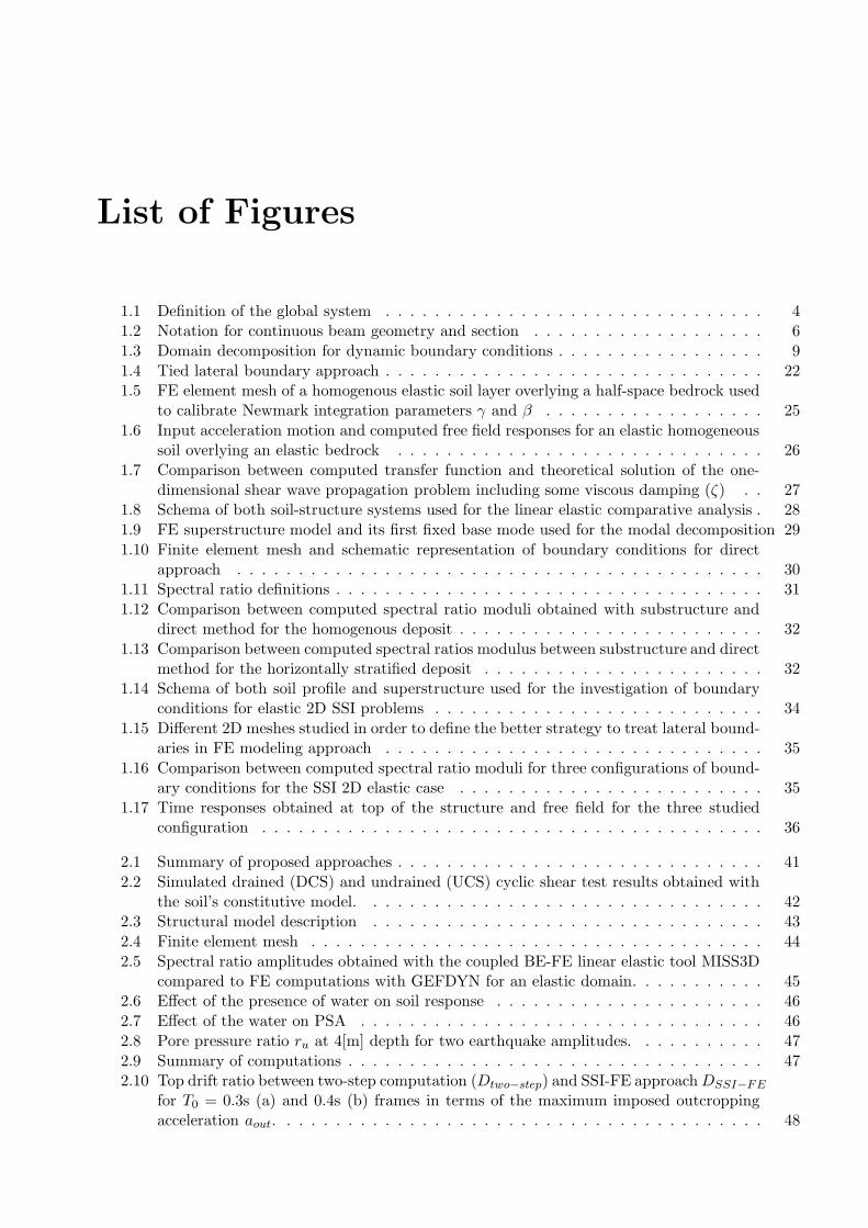
List of Figures
1.1 Definition of the global system . . . . . . . . . . . . . . . . . . . . . . . . . . . . . . . 41.2 Notation for continuous beam geometry and section . . . . . . . . . . . . . . . . . . . 6
1.3 Domain decomposition for dynamic boundary conditions . . . . . . . . . . . . . . . . . 9
1.4 Tied lateral boundary approach . . . . . . . . . . . . . . . . . . . . . . . . . . . . . . . 221.5 FE element mesh of a homogenous elastic soil layer overlying a half-space bedrock used
to calibrate Newmark integration parameters γ and β . . . . . . . . . . . . . . . . . . 25
1.6 Input acceleration motion and computed free field responses for an elastic homogeneoussoil overlying an elastic bedrock . . . . . . . . . . . . . . . . . . . . . . . . . . . . . . 26
1.7 Comparison between computed transfer function and theoretical solution of the one-dimensional shear wave propagation problem including some viscous damping (ζ) . . 27
1.8 Schema of both soil-structure systems used for the linear elastic comparative analysis . 28
1.9 FE superstructure model and its first fixed base mode used for the modal decomposition 29
1.10 Finite element mesh and schematic representation of boundary conditions for directapproach . . . . . . . . . . . . . . . . . . . . . . . . . . . . . . . . . . . . . . . . . . . 30
1.11 Spectral ratio definitions . . . . . . . . . . . . . . . . . . . . . . . . . . . . . . . . . . . 31
1.12 Comparison between computed spectral ratio moduli obtained with substructure anddirect method for the homogenous deposit . . . . . . . . . . . . . . . . . . . . . . . . . 32
1.13 Comparison between computed spectral ratios modulus between substructure and directmethod for the horizontally stratified deposit . . . . . . . . . . . . . . . . . . . . . . . 32
1.14 Schema of both soil profile and superstructure used for the investigation of boundaryconditions for elastic 2D SSI problems . . . . . . . . . . . . . . . . . . . . . . . . . . . 34
1.15 Different 2D meshes studied in order to define the better strategy to treat lateral bound-aries in FE modeling approach . . . . . . . . . . . . . . . . . . . . . . . . . . . . . . . 35
1.16 Comparison between computed spectral ratio moduli for three configurations of bound-ary conditions for the SSI 2D elastic case . . . . . . . . . . . . . . . . . . . . . . . . . 35
1.17 Time responses obtained at top of the structure and free field for the three studiedconfiguration . . . . . . . . . . . . . . . . . . . . . . . . . . . . . . . . . . . . . . . . . 36
2.1 Summary of proposed approaches . . . . . . . . . . . . . . . . . . . . . . . . . . . . . . 41
2.2 Simulated drained (DCS) and undrained (UCS) cyclic shear test results obtained withthe soil’s constitutive model. . . . . . . . . . . . . . . . . . . . . . . . . . . . . . . . . 42
2.3 Structural model description . . . . . . . . . . . . . . . . . . . . . . . . . . . . . . . . 43
2.4 Finite element mesh . . . . . . . . . . . . . . . . . . . . . . . . . . . . . . . . . . . . . 44
2.5 Spectral ratio amplitudes obtained with the coupled BE-FE linear elastic tool MISS3Dcompared to FE computations with GEFDYN for an elastic domain. . . . . . . . . . . 45
2.6 Effect of the presence of water on soil response . . . . . . . . . . . . . . . . . . . . . . 46
2.7 Effect of the water on PSA . . . . . . . . . . . . . . . . . . . . . . . . . . . . . . . . . 46
2.8 Pore pressure ratio ru at 4[m] depth for two earthquake amplitudes. . . . . . . . . . . 47
2.9 Summary of computations . . . . . . . . . . . . . . . . . . . . . . . . . . . . . . . . . . 472.10 Top drift ratio between two-step computation (Dtwo−step) and SSI-FE approachDSSI−FE
for T0 = 0.3s (a) and 0.4s (b) frames in terms of the maximum imposed outcroppingacceleration aout. . . . . . . . . . . . . . . . . . . . . . . . . . . . . . . . . . . . . . . . 48

xiv List of Figures
2.11 Principal strains and the deformed mesh (scaled ×50) in the neighboring saturated soilfor two different steps of analysis for the T0 = 0.3s SDOF. . . . . . . . . . . . . . . . . 49
2.12 Summary of results . . . . . . . . . . . . . . . . . . . . . . . . . . . . . . . . . . . . . . 50
2.13 Geometrical scheme . . . . . . . . . . . . . . . . . . . . . . . . . . . . . . . . . . . . . 50
2.14 Effective period and shear wave velocity values . . . . . . . . . . . . . . . . . . . . . . 51
2.15 Equivalent damping computation. . . . . . . . . . . . . . . . . . . . . . . . . . . . . . 51
2.16 Damage index computation . . . . . . . . . . . . . . . . . . . . . . . . . . . . . . . . . 52
2.17 Computed fragility curves . . . . . . . . . . . . . . . . . . . . . . . . . . . . . . . . . . 54
3.1 Typical regular multistory building model . . . . . . . . . . . . . . . . . . . . . . . . . 57
3.2 Typical axis showing out-of-plane periodicity . . . . . . . . . . . . . . . . . . . . . . . 57
3.3 Proposed approaches . . . . . . . . . . . . . . . . . . . . . . . . . . . . . . . . . . . . . 59
3.4 Low-strain characteristics of studied medium dense sand profile in dry and fully satu-rated conditions . . . . . . . . . . . . . . . . . . . . . . . . . . . . . . . . . . . . . . . . 61
3.5 Finite element meshes (SSI-FE approach) . . . . . . . . . . . . . . . . . . . . . . . . . 62
3.6 Three-dimensional FE meshes for numerical validation . . . . . . . . . . . . . . . . . . 64
3.7 Vertical overstress distribution due to superstructure for b01 on dry soil. Window of20× 12[m] under foundation. Deformation magnification factor=100 . . . . . . . . . . 65
3.8 Vertical overstress distribution due to superstructure for b02 on saturated soil. Windowof 40× 20[m] under foundation. Deformation magnification factor=100 . . . . . . . . . 65
3.9 Degree of mobilization of yz deviatoric mechanism for b02 on dry soil. Window of40× 20[m] under foundation. Deformation magnification factor=100 . . . . . . . . . . 66
3.10 Interface stresses for b01 building on dry soil using modified plane-strain approach and3D model . . . . . . . . . . . . . . . . . . . . . . . . . . . . . . . . . . . . . . . . . . . 66
3.11 Frequency domain responses for b01 building on dry soil using modified plane-strainapproach and 3D model . . . . . . . . . . . . . . . . . . . . . . . . . . . . . . . . . . . 67
3.12 Time domain responses for b01 building on dry soil using modified plane-strain approachand 3D model . . . . . . . . . . . . . . . . . . . . . . . . . . . . . . . . . . . . . . . . . 68
3.13 Time domain shear strain γyz evolution for b01 building on dry soil using modifiedplane-strain approach and 3D model . . . . . . . . . . . . . . . . . . . . . . . . . . . . 68
3.14 Illustration of two-level full factorial design with factors TSR, AI and Tm (adapted fromNIST/SEMATECH (2006)). . . . . . . . . . . . . . . . . . . . . . . . . . . . . . . . . . 69
3.15 ACP analysis of selected input . . . . . . . . . . . . . . . . . . . . . . . . . . . . . . . 71
3.16 Non-linear behavior of the column subjected to the selected earthquakes . . . . . . . . 71
3.17 Effect of overburden pressure in free field response . . . . . . . . . . . . . . . . . . . . 72
3.18 Scatter plots of maximum inter-story drift for b01 building on dry soil . . . . . . . . . 73
3.19 Scatter plots of maximum inter-story drift for b01 building on saturated soil . . . . . . 74
3.20 Comparison between response spectra at the base of the superstructure following T-Sand SSI-FE approaches for b01 building . . . . . . . . . . . . . . . . . . . . . . . . . . 75
3.21 Scatter plots of maximum foundation co-seismic settlement . . . . . . . . . . . . . . . 75
3.22 Scatter plots of maximum inter-story drift for b02 building on dry soil . . . . . . . . . 76
3.23 Scatter plots of maximum inter-story drift for b02 building on saturated soil . . . . . . 76
3.24 Comparison between response spectra at the base of the superstructure following T-Sand SSI-FE approaches for b02 building . . . . . . . . . . . . . . . . . . . . . . . . . . 77
3.25 Scatter plots of energy dissipated by the superstructure for b01 building . . . . . . . . 78
3.26 Scatter plots of energy dissipated by the superstructure for b02 building . . . . . . . . 79
3.27 Definition of the integration volume Ω to compute normalized energy dissipation indexIsoil . . . . . . . . . . . . . . . . . . . . . . . . . . . . . . . . . . . . . . . . . . . . . . 80
3.28 Time domain shear stress-strain responses at three different depths for record number 5 80
3.29 Spatial distribution of hysteretic damping in saturated soil subjected to record number 5 81
3.30 Definition of the integration volume Ω to compute normalized energy dissipation indexIsoil for SSI-FE approach . . . . . . . . . . . . . . . . . . . . . . . . . . . . . . . . . . 81
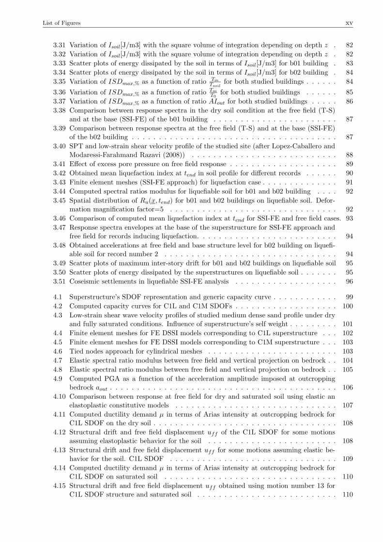
List of Figures xv
3.31 Variation of Isoil[J/m3] with the square volume of integration depending on depth z . 82
3.32 Variation of Isoil[J/m3] with the square volume of integration depending on depth z . 82
3.33 Scatter plots of energy dissipated by the soil in terms of Isoil[J/m3] for b01 building . 83
3.34 Scatter plots of energy dissipated by the soil in terms of Isoil[J/m3] for b02 building . 84
3.35 Variation of ISDmax,% as a function of ratio Tm
Tsoilfor both studied buildings . . . . . . 84
3.36 Variation of ISDmax,% as a function of ratio Tm
T0for both studied buildings . . . . . . 85
3.37 Variation of ISDmax,% as a function of ratio AIout for both studied buildings . . . . . 86
3.38 Comparison between response spectra in the dry soil condition at the free field (T-S)and at the base (SSI-FE) of the b01 building . . . . . . . . . . . . . . . . . . . . . . . 87
3.39 Comparison between response spectra at the free field (T-S) and at the base (SSI-FE)of the b02 building . . . . . . . . . . . . . . . . . . . . . . . . . . . . . . . . . . . . . . 87
3.40 SPT and low-strain shear velocity profile of the studied site (after Lopez-Caballero andModaressi-Farahmand Razavi (2008)) . . . . . . . . . . . . . . . . . . . . . . . . . . . 88
3.41 Effect of excess pore pressure on free field response . . . . . . . . . . . . . . . . . . . . 89
3.42 Obtained mean liquefaction index at tend in soil profile for different records . . . . . . 90
3.43 Finite element meshes (SSI-FE approach) for liquefaction case . . . . . . . . . . . . . . 91
3.44 Computed spectral ratios modulus for liquefiable soil for b01 and b02 building . . . . 92
3.45 Spatial distribution of Ru(x, tend) for b01 and b02 buildings on liquefiable soil. Defor-mation magnification factor=5 . . . . . . . . . . . . . . . . . . . . . . . . . . . . . . . 92
3.46 Comparison of computed mean liquefaction index at tend for SSI-FE and free field cases. 93
3.47 Response spectra envelopes at the base of the superstructure for SSI-FE approach andfree field for records inducing liquefaction. . . . . . . . . . . . . . . . . . . . . . . . . . 94
3.48 Obtained accelerations at free field and base structure level for b02 building on liquefi-able soil for record number 2 . . . . . . . . . . . . . . . . . . . . . . . . . . . . . . . . 94
3.49 Scatter plots of maximum inter-story drift for b01 and b02 buildings on liquefiable soil 95
3.50 Scatter plots of energy dissipated by the superstructures on liquefiable soil . . . . . . . 95
3.51 Coseismic settlements in liquefiable SSI-FE analysis . . . . . . . . . . . . . . . . . . . 96
4.1 Superstructure’s SDOF representation and generic capacity curve . . . . . . . . . . . . 99
4.2 Computed capacity curves for C1L and C1M SDOFs . . . . . . . . . . . . . . . . . . . 100
4.3 Low-strain shear wave velocity profiles of studied medium dense sand profile under dryand fully saturated conditions. Influence of superstructure’s self weight . . . . . . . . . 101
4.4 Finite element meshes for FE DSSI models corresponding to C1L superstructure . . . 102
4.5 Finite element meshes for FE DSSI models corresponding to C1M superstructure . . . 103
4.6 Tied nodes approach for cylindrical meshes . . . . . . . . . . . . . . . . . . . . . . . . 103
4.7 Elastic spectral ratio modulus between free field and vertical projection on bedrock . . 104
4.8 Elastic spectral ratio modulus between free field and vertical projection on bedrock . . 105
4.9 Computed PGA as a function of the acceleration amplitude imposed at outcroppingbedrock aout . . . . . . . . . . . . . . . . . . . . . . . . . . . . . . . . . . . . . . . . . . 106
4.10 Comparison between response at free field for dry and saturated soil using elastic anelastoplastic constitutive models . . . . . . . . . . . . . . . . . . . . . . . . . . . . . . 107
4.11 Computed ductility demand µ in terms of Arias intensity at outcropping bedrock forC1L SDOF on the dry soil . . . . . . . . . . . . . . . . . . . . . . . . . . . . . . . . . . 108
4.12 Structural drift and free field displacement uff of the C1L SDOF for some motionsassuming elastoplastic behavior for the soil . . . . . . . . . . . . . . . . . . . . . . . . 108
4.13 Structural drift and free field displacement uff for some motions assuming elastic be-havior for the soil. C1L SDOF . . . . . . . . . . . . . . . . . . . . . . . . . . . . . . . 109
4.14 Computed ductility demand µ in terms of Arias intensity at outcropping bedrock forC1L SDOF on saturated soil . . . . . . . . . . . . . . . . . . . . . . . . . . . . . . . . 110
4.15 Structural drift and free field displacement uff obtained using motion number 13 forC1L SDOF structure and saturated soil . . . . . . . . . . . . . . . . . . . . . . . . . . 110
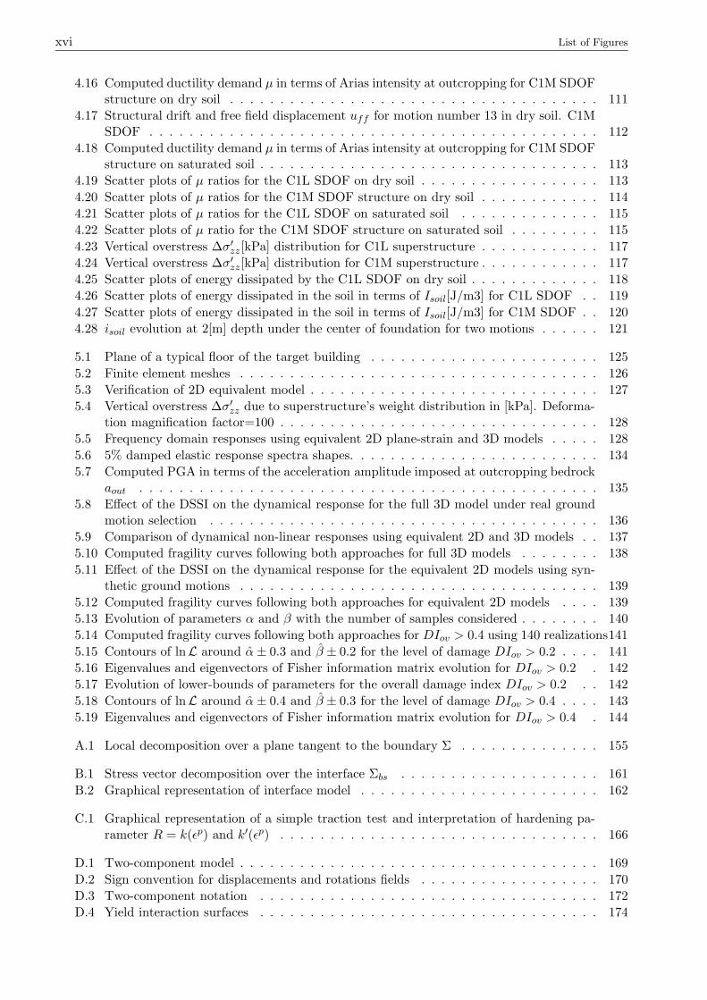
xvi List of Figures
4.16 Computed ductility demand µ in terms of Arias intensity at outcropping for C1M SDOFstructure on dry soil . . . . . . . . . . . . . . . . . . . . . . . . . . . . . . . . . . . . . 111
4.17 Structural drift and free field displacement uff for motion number 13 in dry soil. C1MSDOF . . . . . . . . . . . . . . . . . . . . . . . . . . . . . . . . . . . . . . . . . . . . . 112
4.18 Computed ductility demand µ in terms of Arias intensity at outcropping for C1M SDOFstructure on saturated soil . . . . . . . . . . . . . . . . . . . . . . . . . . . . . . . . . . 113
4.19 Scatter plots of µ ratios for the C1L SDOF on dry soil . . . . . . . . . . . . . . . . . . 113
4.20 Scatter plots of µ ratios for the C1M SDOF structure on dry soil . . . . . . . . . . . . 114
4.21 Scatter plots of µ ratios for the C1L SDOF on saturated soil . . . . . . . . . . . . . . 115
4.22 Scatter plots of µ ratio for the C1M SDOF structure on saturated soil . . . . . . . . . 115
4.23 Vertical overstress ∆σ′zz[kPa] distribution for C1L superstructure . . . . . . . . . . . . 117
4.24 Vertical overstress ∆σ′zz[kPa] distribution for C1M superstructure . . . . . . . . . . . . 117
4.25 Scatter plots of energy dissipated by the C1L SDOF on dry soil . . . . . . . . . . . . . 118
4.26 Scatter plots of energy dissipated in the soil in terms of Isoil[J/m3] for C1L SDOF . . 119
4.27 Scatter plots of energy dissipated in the soil in terms of Isoil[J/m3] for C1M SDOF . . 120
4.28 isoil evolution at 2[m] depth under the center of foundation for two motions . . . . . . 121
5.1 Plane of a typical floor of the target building . . . . . . . . . . . . . . . . . . . . . . . 125
5.2 Finite element meshes . . . . . . . . . . . . . . . . . . . . . . . . . . . . . . . . . . . . 126
5.3 Verification of 2D equivalent model . . . . . . . . . . . . . . . . . . . . . . . . . . . . . 127
5.4 Vertical overstress ∆σ′zz due to superstructure’s weight distribution in [kPa]. Deforma-tion magnification factor=100 . . . . . . . . . . . . . . . . . . . . . . . . . . . . . . . . 128
5.5 Frequency domain responses using equivalent 2D plane-strain and 3D models . . . . . 128
5.6 5% damped elastic response spectra shapes. . . . . . . . . . . . . . . . . . . . . . . . . 134
5.7 Computed PGA in terms of the acceleration amplitude imposed at outcropping bedrockaout . . . . . . . . . . . . . . . . . . . . . . . . . . . . . . . . . . . . . . . . . . . . . . 135
5.8 Effect of the DSSI on the dynamical response for the full 3D model under real groundmotion selection . . . . . . . . . . . . . . . . . . . . . . . . . . . . . . . . . . . . . . . 136
5.9 Comparison of dynamical non-linear responses using equivalent 2D and 3D models . . 137
5.10 Computed fragility curves following both approaches for full 3D models . . . . . . . . 138
5.11 Effect of the DSSI on the dynamical response for the equivalent 2D models using syn-thetic ground motions . . . . . . . . . . . . . . . . . . . . . . . . . . . . . . . . . . . . 139
5.12 Computed fragility curves following both approaches for equivalent 2D models . . . . 139
5.13 Evolution of parameters α and β with the number of samples considered . . . . . . . . 140
5.14 Computed fragility curves following both approaches for DIov > 0.4 using 140 realizations141
5.15 Contours of lnL around α± 0.3 and β ± 0.2 for the level of damage DIov > 0.2 . . . . 141
5.16 Eigenvalues and eigenvectors of Fisher information matrix evolution for DIov > 0.2 . 142
5.17 Evolution of lower-bounds of parameters for the overall damage index DIov > 0.2 . . 142
5.18 Contours of lnL around α± 0.4 and β ± 0.3 for the level of damage DIov > 0.4 . . . . 143
5.19 Eigenvalues and eigenvectors of Fisher information matrix evolution for DIov > 0.4 . 144
A.1 Local decomposition over a plane tangent to the boundary Σ . . . . . . . . . . . . . . 155
B.1 Stress vector decomposition over the interface Σbs . . . . . . . . . . . . . . . . . . . . 161
B.2 Graphical representation of interface model . . . . . . . . . . . . . . . . . . . . . . . . 162
C.1 Graphical representation of a simple traction test and interpretation of hardening pa-rameter R = k(ǫp) and k′(ǫp) . . . . . . . . . . . . . . . . . . . . . . . . . . . . . . . . 166
D.1 Two-component model . . . . . . . . . . . . . . . . . . . . . . . . . . . . . . . . . . . . 169
D.2 Sign convention for displacements and rotations fields . . . . . . . . . . . . . . . . . . 170
D.3 Two-component notation . . . . . . . . . . . . . . . . . . . . . . . . . . . . . . . . . . 172
D.4 Yield interaction surfaces . . . . . . . . . . . . . . . . . . . . . . . . . . . . . . . . . . 174
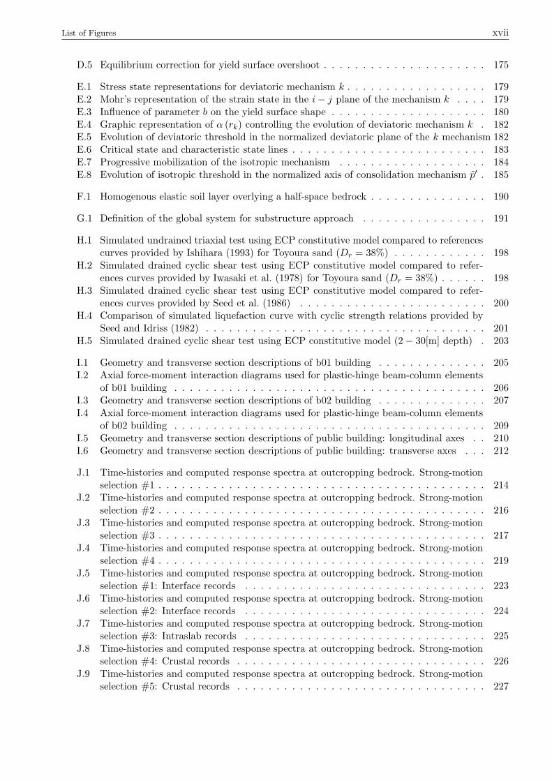
List of Figures xvii
D.5 Equilibrium correction for yield surface overshoot . . . . . . . . . . . . . . . . . . . . . 175
E.1 Stress state representations for deviatoric mechanism k . . . . . . . . . . . . . . . . . . 179E.2 Mohr’s representation of the strain state in the i− j plane of the mechanism k . . . . 179E.3 Influence of parameter b on the yield surface shape . . . . . . . . . . . . . . . . . . . . 180E.4 Graphic representation of α (rk) controlling the evolution of deviatoric mechanism k . 182E.5 Evolution of deviatoric threshold in the normalized deviatoric plane of the k mechanism 182E.6 Critical state and characteristic state lines . . . . . . . . . . . . . . . . . . . . . . . . . 183E.7 Progressive mobilization of the isotropic mechanism . . . . . . . . . . . . . . . . . . . 184E.8 Evolution of isotropic threshold in the normalized axis of consolidation mechanism p′ . 185
F.1 Homogenous elastic soil layer overlying a half-space bedrock . . . . . . . . . . . . . . . 190
G.1 Definition of the global system for substructure approach . . . . . . . . . . . . . . . . 191
H.1 Simulated undrained triaxial test using ECP constitutive model compared to referencescurves provided by Ishihara (1993) for Toyoura sand (Dr = 38%) . . . . . . . . . . . . 198
H.2 Simulated drained cyclic shear test using ECP constitutive model compared to refer-ences curves provided by Iwasaki et al. (1978) for Toyoura sand (Dr = 38%) . . . . . . 198
H.3 Simulated drained cyclic shear test using ECP constitutive model compared to refer-ences curves provided by Seed et al. (1986) . . . . . . . . . . . . . . . . . . . . . . . . 200
H.4 Comparison of simulated liquefaction curve with cyclic strength relations provided bySeed and Idriss (1982) . . . . . . . . . . . . . . . . . . . . . . . . . . . . . . . . . . . . 201
H.5 Simulated drained cyclic shear test using ECP constitutive model (2− 30[m] depth) . 203
I.1 Geometry and transverse section descriptions of b01 building . . . . . . . . . . . . . . 205I.2 Axial force-moment interaction diagrams used for plastic-hinge beam-column elements
of b01 building . . . . . . . . . . . . . . . . . . . . . . . . . . . . . . . . . . . . . . . . 206I.3 Geometry and transverse section descriptions of b02 building . . . . . . . . . . . . . . 207I.4 Axial force-moment interaction diagrams used for plastic-hinge beam-column elements
of b02 building . . . . . . . . . . . . . . . . . . . . . . . . . . . . . . . . . . . . . . . . 209I.5 Geometry and transverse section descriptions of public building: longitudinal axes . . 210I.6 Geometry and transverse section descriptions of public building: transverse axes . . . 212
J.1 Time-histories and computed response spectra at outcropping bedrock. Strong-motionselection #1 . . . . . . . . . . . . . . . . . . . . . . . . . . . . . . . . . . . . . . . . . . 214
J.2 Time-histories and computed response spectra at outcropping bedrock. Strong-motionselection #2 . . . . . . . . . . . . . . . . . . . . . . . . . . . . . . . . . . . . . . . . . . 216
J.3 Time-histories and computed response spectra at outcropping bedrock. Strong-motionselection #3 . . . . . . . . . . . . . . . . . . . . . . . . . . . . . . . . . . . . . . . . . . 217
J.4 Time-histories and computed response spectra at outcropping bedrock. Strong-motionselection #4 . . . . . . . . . . . . . . . . . . . . . . . . . . . . . . . . . . . . . . . . . . 219
J.5 Time-histories and computed response spectra at outcropping bedrock. Strong-motionselection #1: Interface records . . . . . . . . . . . . . . . . . . . . . . . . . . . . . . . 223
J.6 Time-histories and computed response spectra at outcropping bedrock. Strong-motionselection #2: Interface records . . . . . . . . . . . . . . . . . . . . . . . . . . . . . . . 224
J.7 Time-histories and computed response spectra at outcropping bedrock. Strong-motionselection #3: Intraslab records . . . . . . . . . . . . . . . . . . . . . . . . . . . . . . . 225
J.8 Time-histories and computed response spectra at outcropping bedrock. Strong-motionselection #4: Crustal records . . . . . . . . . . . . . . . . . . . . . . . . . . . . . . . . 226
J.9 Time-histories and computed response spectra at outcropping bedrock. Strong-motionselection #5: Crustal records . . . . . . . . . . . . . . . . . . . . . . . . . . . . . . . . 227

xviii List of Figures
Introduction
Motivation
During the last years, significant advances in comprehensive strategies for seismic risk assessmenthave been developed in Earthquake Engineering. Indeed, elaborated methods have been proposedto quantify structural and non-structural damage, to estimate the number of casualties or to predictthe rehabilitation cost after major earthquakes. In this way, powerful analysis methods have beendeveloped to accurately analyze structural models and estimate the demands for different levels ofshaking. Nevertheless, the major part of these methods do not incorporate explicitly the foundationconditions. Thus, the structure is supposed to be clumped on the foundation medium and local soilconditions are solely included by selecting adequate ground motions compatible with the characteristicsof the soil deposit.
Both, research and practice, have shown that a structure founded on a deformable soil couldrespond differently compared to a fixed base situation. Indeed, in flexible supported case, mutualinteraction between structure and adjacent soil takes place inducing modifications in the dynamicresponse. The interaction of the soil with a superstructure has been the subject of numerous inves-tigations assuming linearity of both, superstructure and soil foundation. Nevertheless, the effect ofdynamic soil-structure interaction (DSSI) may differ between elastic and inelastic systems. Thus, thecurrent interaction methodologies based on elastic response studies could not be directly applicable tostructures expected to behave inelastically during severe earthquakes. Additionally, the soil is knownto exhibit non-linear behavior even for relatively weak to moderate ground motions. Consequently,ignoring the non-linear characteristics of the DSSI phenomenon could lead to erroneous predictions ofstructural damage.
In every day engineering practice, static, dynamic or incremental dynamic, non-linear structuralseismic analysis procedures become more and more frequent. In contrast, full non-linear dynamicsoil-structure analysis is still out of the usual practice, and is restricted because of the high com-putational cost of this kind of analysis. Consequently, it is a challenge for researchers to identifyconfigurations where the structural response is highly affected by the non-linear DSSI. As a generalrule, the soil-structure interaction effects are assumed beneficial and ignored. Nevertheless, a moreprecise knowledge of the expected structural seismic response including DSSI effects could allow reducethe cost of new structures with the same reliability and improve the earthquake engineering practice.
Objectives and scope
The goal of this work is to develop a general strategy to address the full non-linear DSSI problem.This strategy includes: the construction of an appropriate numerical model taking into account realistically the physical
phenomena encountered such as the wave propagation and the non-linear behavior of bothsuperstructure and soil, as well the soil-foundation contact problem the selection of an adequate strong motion database

2 List of Figures the identification of a set of suitable measures describing the earthquake, the soil and the struc-ture dynamic responses the inclusion of non-linear DSSI effects into a seismic vulnerability assessment
This work aims to show how realistic Finite Elements (FE) models can be constructed and appliedin a practical way to deal with the issues associated to non-linear DSSI. Some modeling strategiesare introduced and validated in order to reduce the computational cost for a given configuration.Several indicators for both structural and soil responses are developed in order to summarize theirbehavior under seismic loading. Additionally, a vulnerability assessment strategy is presented in termsof measures of information provided by a ground motion selection.
Several single-degree-of-freedom (SDOF) and multiple-degree-of-freedom (MDOF) structures foundedon several soils are studied. In addition, two hydraulic conditions are considered: dry and fully satu-rated. Conclusions, as general as possible, are derived for each case. General tendencies are identifiedin several configurations.
The ultimate goal is to encourage practice towards the inclusion of DSSI phenomena in order toimprove the prediction of the structural response under weak to moderate ground motions. The nearto soil-failure case has been intentionally excluded from the scope of the present work.
Organization and outline
All chapters are written to be autonomous, each planned as a future publication. Some information re-garding theoretical formulation of used constitutive models, considered structures’ details and selectedstrong motions, have been placed in appendices to simplify the lecture of the document.
Chapter 1 establishes and defines the basic principles of the time-domain dynamic soil-structureinteraction problem. The theoretical strong formulation and the corresponding weak formulation fora FE modeling are presented. Generalities about the time and the non-linear integration strategiesadopted in the used tool GEFDyn are also provided. The final part of this chapter describes in detailthe adopted criteria to model the DSSI problem by FE, and presents numerical validations of the usedmodels compared to the results obtained by a coupled BE-FE approach.
Chapter 2 summarizes the earliest stage of this work. The general strategy to define a set ofcomparable data including and neglecting DSSI effects is presented in this chapter. Implicationsof the non-linear DSSI in standard non-linear static procedures for seismic demand assessment areinvestigated. The influence of the DSSI on the seismic structural demand is summarized in terms offragility curves. Three major issues are detected at this stage of the work: limitations associated toa 2D plane-strain approach, contribution of the elastic part of the DSSI and influence of the seismicdatabase on the obtained fragility curves. These issues are explored in detail in Chapters 3, 4 and 5,respectively.
Chapter 3 proposes a modified plane-strain approach to model the non-linear DSSI problemfor regular buildings. Multiple validations are provided to highlight the accuracy of the introducedapproach. A strong motion selection strategy is presented. An energy oriented analysis is introducedto evaluate the response of the soil and the building. Two buildings founded on three different soilsare studied.
Chapter 4 explores the contribution of the elastic DSSI to the complete non-linear DSSI problem.With this purpose, a set of 3D analyses are carried out for two SDOF structures laid on two soils.General tendencies in terms of influence on the ductility demand are presented. Situations whereelastic DSSI considerations give an erroneous prediction are identified.
Chapter 5 introduces a vulnerability assessment strategy in terms of measures of the informationprovided by a ground motion selection. The strategy is applied to a target building over a soil profilecomposed of a mix of sandy and clayey soils. Full 3D and 2D modified plane-strain computations arecarried out. A strategy to construct an equivalent 2D model starting from a 3D regular enough buildingis introduced. A detailed analysis of the influence of the motion database size on the vulnerabilityassessment for the studied case is presented.
Chapter 1
Numerical modeling of non-lineardynamical SSI
Contents
1.1 Introduction . . . . . . . . . . . . . . . . . . . . . . . . . . . . . . . . . . . . . 4
1.2 Definition of the problem . . . . . . . . . . . . . . . . . . . . . . . . . . . . . . 4
1.2.1 Governing equations . . . . . . . . . . . . . . . . . . . . . . . . . . . . . . . . . 4
1.2.2 Boundary and Interface Conditions . . . . . . . . . . . . . . . . . . . . . . . . . 8
1.2.3 Earthquake input and dynamic boundary conditions . . . . . . . . . . . . . . . 9
1.2.4 Variational formulation . . . . . . . . . . . . . . . . . . . . . . . . . . . . . . . 10
1.2.5 Space discretization . . . . . . . . . . . . . . . . . . . . . . . . . . . . . . . . . 12
1.2.6 Time discretization . . . . . . . . . . . . . . . . . . . . . . . . . . . . . . . . . . 14
1.2.7 Resolution of non-linear system . . . . . . . . . . . . . . . . . . . . . . . . . . . 17
1.3 Non-linear constitutive models . . . . . . . . . . . . . . . . . . . . . . . . . . 18
1.3.1 Mechanical interfaces . . . . . . . . . . . . . . . . . . . . . . . . . . . . . . . . 19
1.3.2 Continuous non-linear beam model . . . . . . . . . . . . . . . . . . . . . . . . . 19
1.3.3 Plastic hinges beam model . . . . . . . . . . . . . . . . . . . . . . . . . . . . . 19
1.3.4 Constitutive modeling of the soil . . . . . . . . . . . . . . . . . . . . . . . . . . 20
1.3.5 General remarks . . . . . . . . . . . . . . . . . . . . . . . . . . . . . . . . . . . 21
1.4 Special aspects of the numerical resolution of the dynamic SSI problemwith Finite Elements . . . . . . . . . . . . . . . . . . . . . . . . . . . . . . . . 22
1.4.1 One-dimensional ground amplification problem and numerical damping . . . . 23
1.4.2 3D linear elastic SSI numerical validation . . . . . . . . . . . . . . . . . . . . . 27
1.4.3 Investigation of boundary conditions modeling for elastic 2D SSI problem . . . 33
1.5 Concluding remarks . . . . . . . . . . . . . . . . . . . . . . . . . . . . . . . . . 37
4 1.1. Introduction
1.1 Introduction
The assessment of the dynamical soil-structure interaction phenomenon demands the study of severalaspects of the problem, among others: the definition of the seismic hazard, site topography andground water level, the non-linear soil behavior of the soil under cyclic loading, the spatial variationof the soil properties, the non-linear dynamic soil response of the superstructure and the wave patternmodification due to neighboring structures. Nevertheless, several simplifications must be done in orderto formulate a problem which can be solved with the today’s state of the art earthquake engineeringnumerical methods.
In §1.2 a brief review of the governing equations of the dynamical soil-structure problem in view ofa material non-linear finite element numerical implementation is presented. Afterwards, some simpli-fications introduced for the numerical modeling in earthquake engineering practice will be presented.Section 1.3 presents the theoretical formulation and the implementation of the different constitutivemodels used to take into account the material non-linear behavior of the different constituents of theproblem. Finally, §1.4 presents some special aspects of the numerical resolution of the dynamical non-linear soil-structure interaction problem using the Finite Element Method. Some numerical validationof the used finite element tool (GEFDyn ) under linear elastic behavior assumption is also presentedin this section.
1.2 Definition of the problem
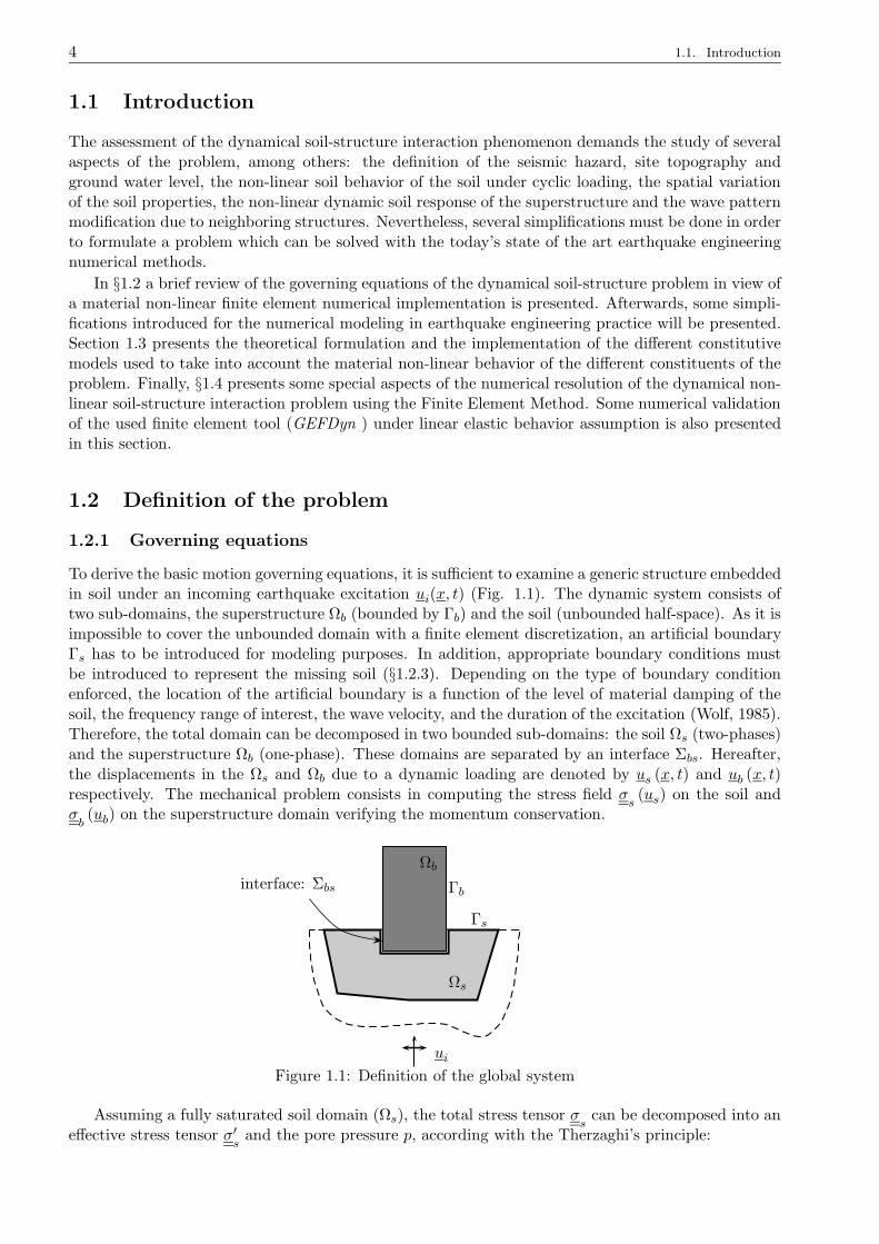
1.2.1 Governing equations
To derive the basic motion governing equations, it is sufficient to examine a generic structure embeddedin soil under an incoming earthquake excitation ui(x, t) (Fig. 1.1). The dynamic system consists oftwo sub-domains, the superstructure Ωb (bounded by Γb) and the soil (unbounded half-space). As it isimpossible to cover the unbounded domain with a finite element discretization, an artificial boundaryΓs has to be introduced for modeling purposes. In addition, appropriate boundary conditions mustbe introduced to represent the missing soil (§1.2.3). Depending on the type of boundary conditionenforced, the location of the artificial boundary is a function of the level of material damping of thesoil, the frequency range of interest, the wave velocity, and the duration of the excitation (Wolf, 1985).Therefore, the total domain can be decomposed in two bounded sub-domains: the soil Ωs (two-phases)and the superstructure Ωb (one-phase). These domains are separated by an interface Σbs. Hereafter,the displacements in the Ωs and Ωb due to a dynamic loading are denoted by us (x, t) and ub (x, t)respectively. The mechanical problem consists in computing the stress field σ
s(us) on the soil and
σb(ub) on the superstructure domain verifying the momentum conservation.
Ωs
Γs
interface: Σbs
Ωb
Γb
uiFigure 1.1: Definition of the global system
Assuming a fully saturated soil domain (Ωs), the total stress tensor σs
can be decomposed into aneffective stress tensor σ′
sand the pore pressure p, according with the Therzaghi’s principle:
Chapter 1. Numerical modeling of non-linear dynamical SSI 5
σs
= σ′s− p.I (1.1)
where I is the second-order identity tensor. In (1.1) the continuum mechanic’s sign convention isassumed, i.e. tractions are positive. This decomposition is strictly correct only if the increment of porepressure for a constant effective stress does not deforms the soil’s skeleton. The complete formulationof the problem for the soil domain includes the conservation relations, the constitutive model, theboundary and the initial conditions. Biot (1962) formulated for the first time the dynamic behavior ofsaturated porous media. The latter author generalized the consolidation theory to three dimensionalcase and introduced the inertia forces and the compressibility of pore water, but did not include theTerzaghi’s principle in his formulation. The mathematical formulation of the complete problem can bedone using several choices of dependant variables. Either, the absolute displacements of the solid andof the fluid and the pressure (us, uf , p) (Zienkiewicz and Shiomi, 1984) or the absolute displacementsof the solid, the relative displacement of the fluid and the pressure (us, urf , p) (Modaressi, 1987; Aubryand Modaressi, 1992b) can be used. These approaches are interesting for higher frequencies. However,for the frequency range suited in earthquake engineering some simplifications are possible. Zienkiewiczet al. (1980) proposed a simplified formulation of Biot’s equation in dynamics (us − p formulation)for low-frequency range. In this approach, the relative acceleration of the fluid to the solid phase isneglected resulting in a reduction of unknowns. In this case, the momentum conservation may bewritten as:
div σ′s− grad p+ ρ g = ρ us (1.2)
where us is the absolute acceleration vector of the solid skeleton and ρ is the mean soil’s specific mass:
ρ = (1− n) ρs + nρf (1.3)
where n is the porosity, ρs the density of the solid phase and ρf the density of the fluid.
The movement of one phase with respect to the other is controlled by the flow equation (generalizedDarcy’s law) for the simplified us − p approach:
urf = K.(−grad p+ ρf
(g − ρ us
))(1.4)
where urf is the relative velocity vector between the solid phase and the fluid: urf = n(uf − us
)and
K is the permeability tensor:
K =k
ρf .g(1.5)
in which k is the kinematic permeability tensor.
The combination of the mass conservation for each phase gives the following expression:
div urf + div us = −n p
Kf− (1− n)
p
Ks(1.6)
where Kf and Ks are the compressibility of the fluid and the solid skeleton, respectively. Using (1.4)the relative displacement of the fluid may be eliminated:
div us − div(K.grad
(p− ρfg.x
))− div
(K.ρf us
)+p
Q= 0 (1.7)
so that the solid phase displacement and the pore pressure are the only unknown variables. Thecompressibility parameter Q is given by:
1
Q=
n
Kf+ (1− n)
1
Ks(1.8)
6 1.2. Definition of the problem
The main advantage of the simplified model is related to the reduction of the numerical cost. Forexample, for a 3D finite element model the number of degrees of freedom at each node, in the soildomain Ωs, is reduced from 6 to 4. The inaccuracies of the us− p simplified approach are pronouncedonly in high-frequency, short-duration phenomena (Zienkiewicz et al., 1999). The limits of validityof this approach are extensively studied by Zienkiewicz et al. (1980, 1999) following a comparativeone-dimensional analysis between the complete and the approximative formulation and the undrainedcase assuming linear elastic soil’s skeleton behavior.
In summary, the two sets of equations which describe together with the initial and boundaryconditions (§1.2.2) the us − p formulation for the two-phases soil domain Ωs are given by:
div σ′s− grad p+ ρ g = ρus ∀x ∈ Ωs (1.9)
div us − div(K.grad
(p− ρfg.x
))− div
(ρf K.us
)+p
Q= 0 ∀x ∈ Ωs (1.10)
to this one should add the constitutive model (§1.3.4) for the soil skeleton.
It is also necessary to take into account the interaction between the two deformable domains bywriting the conditions of compatibility over the interface Σbs (§1.2.2).
The equilibrium equation for the superstructure domain (Ωb) can be written as:
div σb+ ρb g = ρbub ∀x ∈ Ωb (1.11)
where g is the acceleration of gravity and ρb the specific mass of the superstructure material.
b
b
er
es
et
b
p0
bp∗
b
b
b
x0
b
x∗
u0
u
Figure 1.2: Notation for continuous beam geometry and section
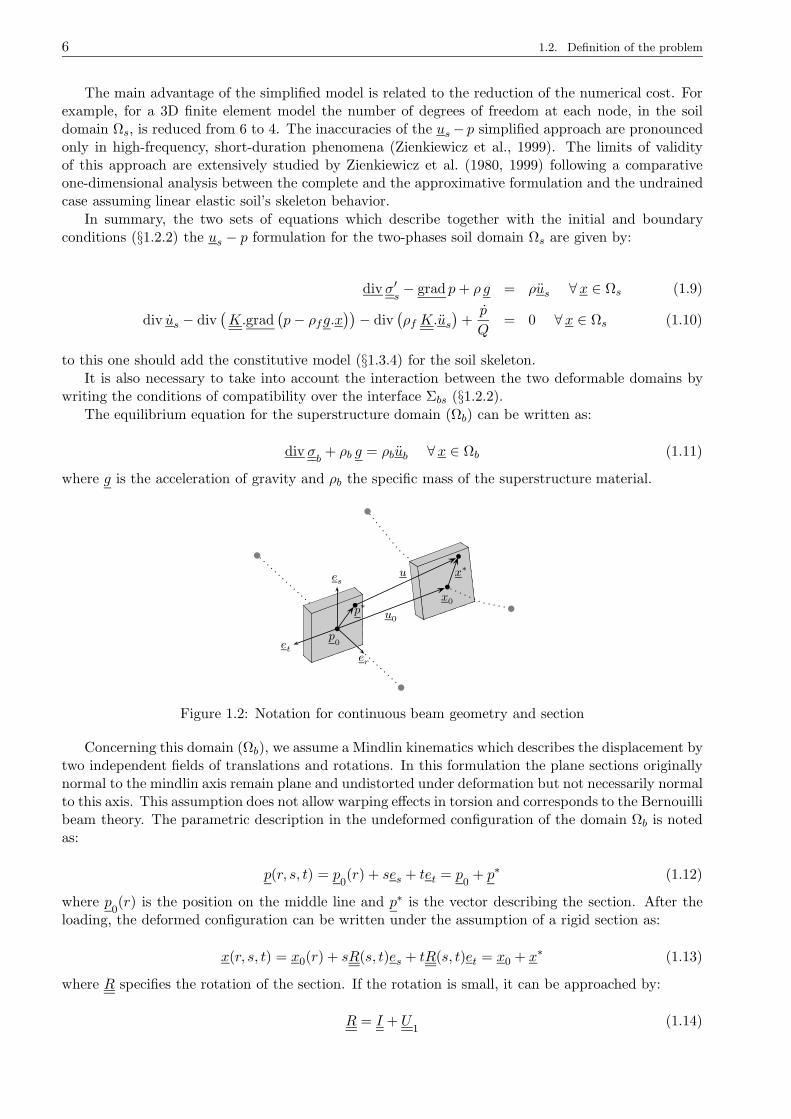
Concerning this domain (Ωb), we assume a Mindlin kinematics which describes the displacement bytwo independent fields of translations and rotations. In this formulation the plane sections originallynormal to the mindlin axis remain plane and undistorted under deformation but not necessarily normalto this axis. This assumption does not allow warping effects in torsion and corresponds to the Bernouillibeam theory. The parametric description in the undeformed configuration of the domain Ωb is notedas:
p(r, s, t) = p0(r) + ses + tet = p
0+ p∗ (1.12)
where p0(r) is the position on the middle line and p∗ is the vector describing the section. After the
loading, the deformed configuration can be written under the assumption of a rigid section as:
x(r, s, t) = x0(r) + sR(s, t)es + tR(s, t)et = x0 + x∗ (1.13)
where R specifies the rotation of the section. If the rotation is small, it can be approached by:
R = I + U1
(1.14)

Chapter 1. Numerical modeling of non-linear dynamical SSI 7
where U1
is antisymmetric. The displacement field in Ωb is given by:
ub = x− p (1.15)
so that:
ub(r, s, t) = u0(r) + sU1(r)es + t U
1(r)et = u0 + U
1x∗ (1.16)
Therefore, the kinematic of the Ωb domain is dependent of only two variables, the vector field u0(r)along the displacement axis and the small rotations antisymmetric operator U
1(r). The operator U
1is associated to a rotation vector u1 by a wedge product:
ub = u0 + u1 ∧ x∗ (1.17)
The gradient of the displacement field can be computed as:
gradub = ∂rub ⊗ er + ∂sub ⊗ es + ∂tub ⊗ et (1.18)
According to the kinematics defined by (1.16), the gradient can be written as:
gradub =(
∂ru0 + ∂rU1.x∗)
⊗ er + U1(es ⊗ es) + U
1(et ⊗ et)
=(
∂ru0 + ∂rU1.x∗)
⊗ er + U1
(I − er ⊗ er
)
= (∂rub − u1 ∧ er)⊗ er + U1
(1.19)
The strain tensor ε is related to ub by:
ε (ub) =1
2
(
gradub + grad utb
)
(1.20)
Using the previous definitions, and using the antisymmetric property of U1, the strain tensor
becomes:
ε (ub) = (∂rub − u1 ∧ er)⊗s er =(
∂ru0 − U1er + ∂rU1
x∗)
⊗s er (1.21)
Expanding the previous expression, we obtain:
ε (ub) =(
∂ru0r +(
∂rU1x∗)
.er
)
er ⊗ er +(
∂ru0.es −(
U1er
)
.es +(
∂rU1x∗)
.es
)
es ⊗s er+(
∂ru0.et −(
U1er
)
.et +(
∂rU1x∗)
.et
)
et ⊗s er (1.22)
We verify that εss = εtt = εst = 0, which means that no deformation within each transverse sectionexist. It is possible to identify the following terms
∂ru0r : axial strain
∂ru0.eα −(
U1er
)
.eα with α = s, t : transverse shear strain(
∂rU1x∗)
.er = (∂ru1 ∧ x∗) .er : bending strain(
∂rU1x∗)
.eα = (∂ru1 ∧ x∗) .eα with α = s, t : torsional strain
The hypothesis of Bernouilli is adopted, i.e. it is assumed the orthogonality of the section withrespect to the deformed midline. This assumption implies that the transverse shear is zero:
8 1.2. Definition of the problem
∂ru0.eα −(
U1er
)
.eα = 0 with α = s, t (1.23)
In this case, the rotation associated with the bending can be expressed from the displacement ofthe axis:
er ∧ (∂r (u0.es) es + ∂r (u0.et) et) = er ∧ (u1 ∧ er) = u1 − u1rer (1.24)
from which:
u1 = er ∧ (∂r (u0.es) es + ∂r (u0.et) et) + u1rer (1.25)
Replacing in the bending strain expression:
∂rU1x∗ = ∂ru1 ∧ x∗
= (er ∧ (∂rr (u0.es) es + ∂rr (u0.et) et) + ∂ru1rer) ∧ x∗
= − (x∗. (∂rr (u0.es) es + ∂rr (u0.et) et)) er + ∂ru1rer ∧ x∗ (1.26)
And finally, the strain tensor can be written as:
ε (ub) = (∂ru0rer + ∂ru1 ∧ x∗)⊗s e3= ((∂ru0r − x∗. (∂rr (u0.es) es + ∂rr (u0.et) et)) er + ∂ru1re3 ∧ x∗)⊗s er (1.27)
Therefore, the movement can be described by the vector field u0 and the twisting component u1r ,both function of the spatial variable r.
1.2.2 Boundary and Interface Conditions
The boundary conditions for the soil domain Ωs will be more complex than for the superstructuredomain Ωb because they must be decomposed into boundary conditions relative to the solid phase andin fluid flow.
For the superstructure, a traction boundary condition is applied (free surface in dynamics):
tb (x, t) = σb. n = 0 ∀x ∈ Γbσ = Γb (1.28)
where tb is the stress vector following the exterior normal direction n of Γb. For some static com-putations, this boundary condition is slightly modified using prescribed values for tractions t∗ over aportion of the boundary Γ∗
bσ(Γ∗bσ∩ Γbσ = ∅ and Γ∗
bσ∪ Γbσ = Γb ):
tb (x) = 0 ∀x ∈ Γbσ
tb (x) = t∗ (x) ∀x ∈ Γ∗bσ
(1.29)
Because of the equations (1.9) and (1.10), the boundary Γs of the domain Ωs is decomposed intotwo types of partitioning. First (1.9) into two parts (mechanical boundary): Γsσ and Γsu . On Γsu thedisplacement is imposed while the total traction boundary condition is retaining on Γsσ (Γsu ∩Γsσ = ∅and Γsu ∪ Γsσ = Γs). For the fluid flow boundary conditions, another partition is considered: Γsp andΓsϕ (Γsp ∩ Γsϕ = ∅ and Γsp ∪ Γsϕ = Γs). On Γp there is a pore pressure boundary condition while onΓsϕ there is a condition on the flux:
urf (x, t) .n = ϕ∗ (x, t) ∀x ∈ Γsϕ (1.30)
where n is the exterior normal vector over Γsϕ and ϕ∗ the prescribed value of the flux.

Chapter 1. Numerical modeling of non-linear dynamical SSI 9
Over the interface Σbs between both domains, the condition on the fluid can be either restrictedto the nullity of the fluid flow through the interface:
(K . grad p(x, t)
). n = 0 ∀x ∈ Σbs (1.31)
or the atmospheric pressure. n is the exterior normal vector of Ωs over the interface Σbs. The continuityof the stress vector must be verified over the interface (even if uplift appears):
tb (x, t) + ts (x, t) = 0 ∀x ∈ Σbs (1.32)
in which ts is the stress vector applied on Γs. Concerning the displacement, discontinuities are allowedbetween Ωs and Ωb over the interface Σbs. If [·] represents the jump of a quantity, the jump ofdisplacements between the superstructure and the soil on the interface Σbf can written as:
[u(x, t)] = ub(x, t)− us(x, t) ∀x ∈ Σbs (1.33)
1.2.3 Earthquake input and dynamic boundary conditions
The specification of the earthquake input motion for a fixed base structure problem is usually doneby prescribing the base displacement ug(t) or base acceleration ug(t). In this approach, the problemis usually formulated in terms of the displacement relative to this base movement, but can be alsoformulated in terms of the total displacements.
Ωs′
Γs′
Ωs
Σ
Ωst
Σbs
ui
Figure 1.3: Domain decomposition for dynamic boundary conditions
In the case of an earthquake non-linear SSI problem treated by a finite elements approach, where atruncated portion of the surrounding soil is added to the problem, the fixed base procedure is strictlynot applicable. In this case, the soil truncation boundary must allow the incoming seismic wave toenter to the model, as well as to ensure that the outgoing waves are transmitted. In order to formulatean appropriate absorbing/incident boundary model, the total unbounded soil domain can be dividedin two distinct sub-domains Ωs and Ωs′ (Fig. 1.3). The domain Ωs is non-linear and two phase, andobeys the equations of the previous sections. The domains Ωs′ is assumed to be elastic, homogenous,isotropic, monophasic and unbounded. The behavior of this last will be modelled by the paraxialapproximation of the elastodynamics equations (Modaressi, 1987; Engquist and Majda, 1977). If thedisplacement field in Ωs′ is denoted by us′ , the equation of elastodynamics in time domain can bewritten as:
(λ+ µ) grad (divus′) + µ us′ = ρs′ us′ ∀x ∈ Ωs′ (1.34)
where λ and µ are the Lame elastic constants and ρs′ the mass density. Free field conditions aresupposed on the boundary Γs′ of Ωs′ . The displacement field us′ must tend to incident field ui farenough from the interface Σ between Ωs and Ωs′ :
lim‖x‖→∞
us′ = ui (1.35)
10 1.2. Definition of the problem
The stress tensor on Ωs′ can be decomposed in a static part σ0s′
due to gravity and static loads,and a dynamic part due to us′ :
σs′
= σ0s′
+ σs′
(us′) (1.36)
At the interface Σ, the continuity of the displacements and the stress vector must be respected:
us′ = us and ts + ts′ (us′) = 0 (1.37)
It is assumed that an elastic monophasic transition soil portion Ωst exists between Σ and Ωs
(Fig. 1.3). This sub-domain obeys the elastodynamics equations. Finally, the initial conditions forunbounded domain Ωs′ are:
us′ (0) = 0
σs′
(0) = σ0s′
us′ (0) = 0 (1.38)
Several authors have proposed perfectly boundary conditions for general classes of wave propaga-tion problems. Unfortunately, these boundary conditions are necessarily nonlocal in both space andtime, and thus are not useful for practical calculations in time domain. In time domain, the simplersolution is to use viscous dampers, but the efficacy of this approach decays when the outgoing waveis not perfectly normal to the damper orientation. Additionally, a total displacement splitting in anincoming wave and the displacement relative to the incoming displacement must be done for earth-quake incident fields problems (Zienkiewicz et al., 1988). The paraxial approximation (Engquist andMajda, 1977), allows to develop a local dynamic impedance in time and space on the interface Σ. Thiskind of boundary approximation can be easily extended to be used simultaneously as an absorbingboundary and as a tool to impose an incident field (Modaressi, 1987). Details about the derivation ofthe paraxial approximation implemented in GEFDyn are provided in the Appendix A.
1.2.4 Variational formulation
The weak form of the governing equations can be obtained using a variational formulation. The setof kinematically acceptable displacement fields Vb for the Ωb domain is defined as:
Vb = wb |wb regular in Ωb , wb(x) = 0 on ΓbuSimilarly, for the Ωs domain a set of acceptable kinematically displacement fields Vs and a set of
admissible pressure fields Q can be defined:
Vs = ws |ws regular in Ωs , ws(x) = 0 on ΓsuQ =
q | q regular in Ωs , q(x) = 0 on Γsp
Considering the previous definitions, the variational formulation of (1.11) can be written as:
∫
Ωb
σb: ε
b(wb) dV +
∫
Ωb
ρbub.wbdV =
∫
Ωb
ρb g.wbdV +
∫
Σbs
tb.wbdS +
∫
Γbσ
tb.wbdS (1.39)
using the Stoke’s formula and the boundary conditions described in the previous section. Accordingto (1.28), the last term vanishes for the dynamic case. ε
bis the strain tensor associated to the virtual
displacement field wb. Using the kinematics imposed for the displacement field:
wb(r, s, t) = w0(r) + w1(r) ∧ x∗ (1.40)
Chapter 1. Numerical modeling of non-linear dynamical SSI 11
the inertia term in (1.39) can be computed as:
∫
Ωb
ρb ub.wbdV =
∫
L
∫
S
ρb (u0 + u1 ∧ x∗) . (w0 + w1 ∧ x∗) dSdl
=
∫
L
ρ u0.w0 + ρx. (u0 ∧ w1 − u1 ∧ w0) +(J u1
).w1 dl (1.41)
where dl and dS indicates integration following the midline and over the section, respectively. Themass density per unit of length (ρ), the center of inertia of the section x and the inertia operator ofthe section (J) are defined by:
ρ =
∫
S
ρb dS ; ρx =
∫
S
ρbx∗ dS and J =
∫
S
ρ(
|x∗|2 I − x∗ ⊗ x∗)
dS
If the inertia center of the section is not on the midline, coupling effects appears between axial andbending fields. The integration of internal force term can be also decomposed into the axial directionand over the section. Using the imposed kinematics and the symmetry of the stress tensor, it can bewritten as:
∫
Ωb
σb: ε (wb) dV =
∫
L
∫
S
(
σber
)
. (∂rwb −w1 ∧ er) dSdl
=
∫
L
∫
S
(
−er ∧(
σber
))
.w1 +(
σber
)
.∂rwb dSdl
=
∫
L
(−er ∧ q
).w1 + q.∂rw0 +m.∂rw1 dl (1.42)
where q and m are the resultant force and the bending moment over the section:
q =
∫
S
σber dS and m =
∫
S
x∗ ∧(
σber
)
dS
The body forces can be computed by a similar way:
∫
Ωb
ρbg.wb dV =
∫
L
∫
S
ρg. (w0 + w1 ∧ x∗) dSdl
= ρ
∫
L
∫
S
g.w0 +(x∗ ∧ g
).w1 dSdl
=
∫
L
qg.w0 +mg.w1 dl (1.43)
where qg
and mg are the section equivalent forces and moments due to body forces:
qg
=
∫
S
ρb g dS and mg =
∫
S
ρb x∗ ∧ g dS
Similarly, the variational formulation for the soil domain (1.10) is given by:
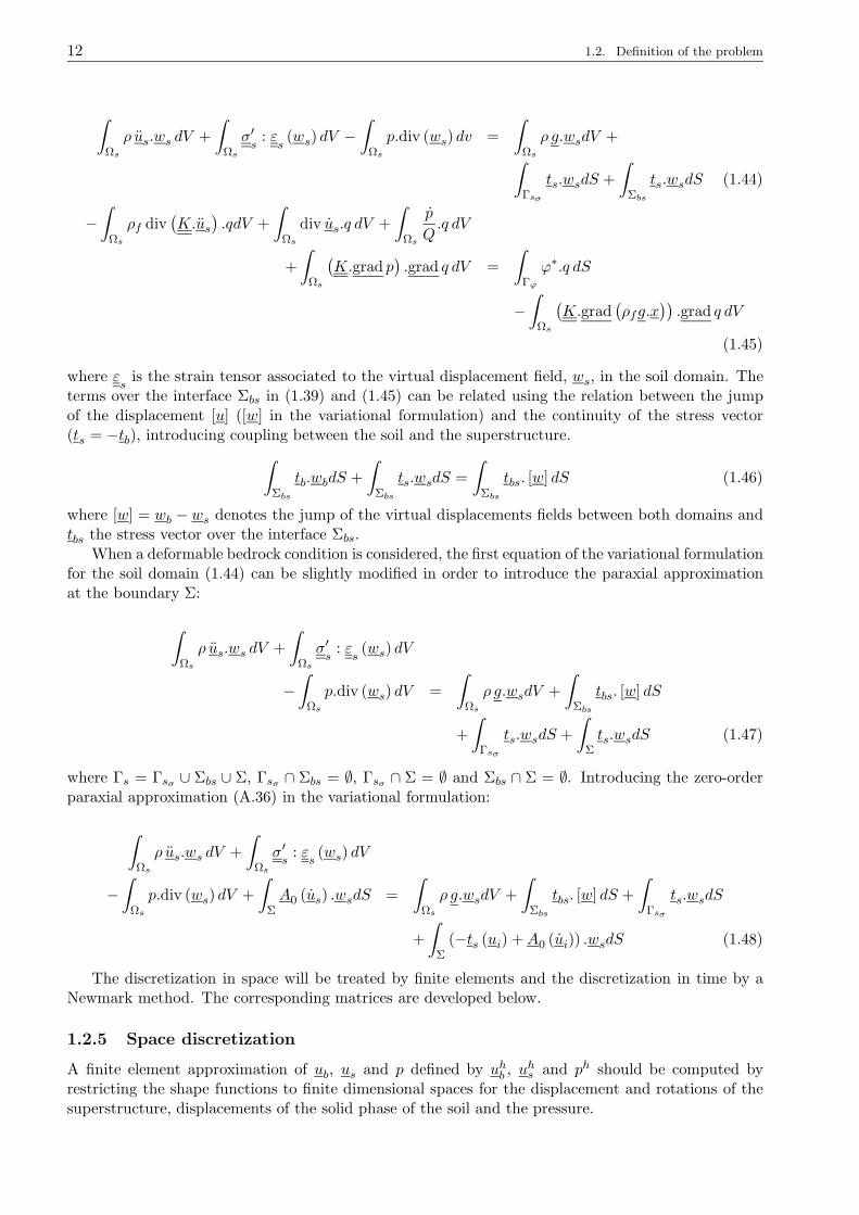
12 1.2. Definition of the problem
∫
Ωs
ρ us.ws dV +
∫
Ωs
σ′s
: εs(ws) dV −
∫
Ωs
p.div (ws) dv =
∫
Ωs
ρ g.wsdV +
∫
Γsσ
ts.wsdS +
∫
Σbs
ts.wsdS (1.44)
−∫
Ωs
ρf div(K.us
).qdV +
∫
Ωs
div us.q dV +
∫
Ωs
p
Q.q dV
+
∫
Ωs
(K.grad p
).grad q dV =
∫
Γϕ
ϕ∗.q dS
−∫
Ωs
(K.grad
(ρfg.x
)).grad q dV
(1.45)
where εs
is the strain tensor associated to the virtual displacement field, ws, in the soil domain. Theterms over the interface Σbs in (1.39) and (1.45) can be related using the relation between the jumpof the displacement [u] ([w] in the variational formulation) and the continuity of the stress vector(ts = −tb), introducing coupling between the soil and the superstructure.
∫
Σbs
tb.wbdS +
∫
Σbs
ts.wsdS =
∫
Σbs
tbs. [w] dS (1.46)
where [w] = wb − ws denotes the jump of the virtual displacements fields between both domains andtbs the stress vector over the interface Σbs.
When a deformable bedrock condition is considered, the first equation of the variational formulationfor the soil domain (1.44) can be slightly modified in order to introduce the paraxial approximationat the boundary Σ:
∫
Ωs
ρ us.ws dV +
∫
Ωs
σ′s
: εs(ws) dV
−∫
Ωs
p.div (ws) dV =
∫
Ωs
ρ g.wsdV +
∫
Σbs
tbs. [w] dS
+
∫
Γsσ
ts.wsdS +
∫
Σts.wsdS (1.47)
where Γs = Γsσ ∪ Σbs ∪ Σ, Γsσ ∩ Σbs = ∅, Γsσ ∩ Σ = ∅ and Σbs ∩ Σ = ∅. Introducing the zero-orderparaxial approximation (A.36) in the variational formulation:
∫
Ωs
ρ us.ws dV +
∫
Ωs
σ′s
: εs(ws) dV
−∫
Ωs
p.div (ws) dV +
∫
ΣA0 (us) .wsdS =
∫
Ωs
ρ g.wsdV +
∫
Σbs
tbs. [w] dS +
∫
Γsσ
ts.wsdS
+
∫
Σ(−ts (ui) +A0 (ui)) .wsdS (1.48)
The discretization in space will be treated by finite elements and the discretization in time by aNewmark method. The corresponding matrices are developed below.
1.2.5 Space discretization
A finite element approximation of ub, us and p defined by uhb , uhs and ph should be computed by
restricting the shape functions to finite dimensional spaces for the displacement and rotations of thesuperstructure, displacements of the solid phase of the soil and the pressure.
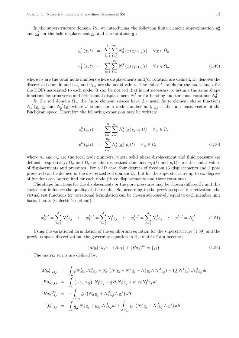
Chapter 1. Numerical modeling of non-linear dynamical SSI 13
In the superstructure domain Ωb, we introducing the following finite element approximation uh0and uh1 for the field displacement u0 and the rotations u1:
uh0 (x, t) =
3∑
i=1
nb∑
I=1
N I0 (x) eiu0Ii
(t) ∀x ∈ Ωb
uh1 (x, t) =3∑
i=1
nb∑
I=1
N I1 (x) eiu1Ii
(t) ∀x ∈ Ωb (1.49)
where nb are the total node numbers where displacements and/or rotation are defined, Ωb denotes thediscretized domain and u0Ii
and u1Iiare the nodal values. The index I stands for the nodes and i for
the DOFs associated to each node. It can be noticed that is not necessary to assume the same shapefunctions for transverse and extensional displacement N I
1 or for bending and torsional rotations N I0 .
In the soil domain Ωs, the finite element spaces have the usual finite element shape functionsNJs (x) .ej and NJ
p (x) where J stands for a node number and, ej is the unit basis vector of theEuclidean space. Therefore the following expansion may be written:
uhs (x, t) =
3∑
i=1
ns∑
I=1
N Is (x) ei uIi(t) ∀x ∈ Ωs
ph (x, t) =
np∑
I=1
N Ip (x) pI(t) ∀x ∈ Ωs (1.50)
where ns and np are the total node numbers, where solid phase displacement and fluid pressure aredefined, respectively; Ωb and Ωs are the discretized domains; uIi(t) and pI(t) are the nodal valuesof displacements and pressures. For a 3D case, four degrees of freedom (3 displacements and 1 porepressure) can be defined in the discretized soil domain Ωs, but for the superstructure up to six degreesof freedom can be required for each node (three displacements and three rotations).
The shape functions for the displacements or the pore pressures may be chosen differently and thischoice can influence the quality of the results. So, according to the previous space discretization, thevirtual test functions for variational formulation can be chosen successively equal to each member unitbasis, that is (Galerkin’s method):
wh,J0 =3∑
j=1
NJ0 ej ; wh,J1 =
3∑
j=1
NJ1 ej ; wh,Js =
3∑
j=1
NJb ej ; ph,J = NJ
p (1.51)
Using the variational formulation of the equilibrium equation for the superstructure (1.39) and theprevious space discretization, the governing equation in the matrix form becomes:
[Mbb] ub+ Bσb+ Bσbbs = fb (1.52)
The matrix terms are defined by:
[Mbb]IiJj =
∫
L
ρN I0 ei.N
J0 ej + ρx.
(N I
0 ei ∧NJ1 ej −N I
1 ei ∧NJ0 ej)
+(J.N I
1 ei).NJ
1 ej dl
BσbJj =
∫
L
(−er ∧ q
).NJ
1 ej + q.∂rNJ0 ej +m.∂rN
J1 ej dl
BσbbsJj = −∫
Σbs
tb.(NJ
0 ej +NJ1 ej ∧ x∗
)dS
fbJj =
∫
L
qg.NJ
0 ej +mg.NJ1 ejdl +
∫
Γbσ
tb.(NJ
0 ej +NJ1 ej ∧ x∗
)dS
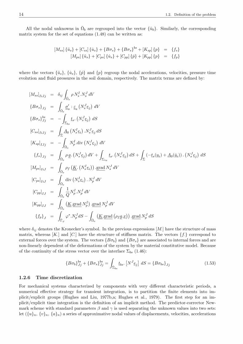
14 1.2. Definition of the problem
All the nodal unknowns in Ωb are regrouped into the vector ub. Similarly, the correspondingmatrix system for the set of equations (1.48) can be written as:
[Mss] us+ [Css] us+ Bσs+ Bσsbs + [Ksp] p = fs[Mps] us+ [Cps] us+ [Cpp] p+ [Kpp] p = fp
where the vectors us, us, p and p regroup the nodal accelerations, velocities, pressure timeevolution and fluid pressures in the soil domain, respectively. The matrix terms are defined by:
[Mss]IiJj = δij
∫
Ωs
ρN Is .N
Js dV
BσsJj =
∫
Ωs
σ′s
: εs
(NJs ej)dV
BσsbsJj = −∫
Σbs
ts.(NJs ej)dS
[Css]IiJj =
∫
ΣA0
(N Is ei).NJ
s ej dS
[Ksp]IJj = −∫
Ωs
N Ip .div
(NJs ej)dV
fsJj =
∫
Ωs
ρ g.(NJs ej)dV +
∫
Σsσ
ts.(NJs ej)dS +
∫
Σ(−ts(ui) +A0(ui)) .
(NJs ej)dS
[Mps]IiJ =
∫
Ωs
ρf(K.(N Is ei)).gradNJ
s dV
[Cps]IiJ =
∫
Ωs
div(N Is ei). NJ
p dV
[Cpp]IJ =
∫
Ωs
1
QN Ip .N
Jp dV
[Kpp]IJ =
∫
Ωs
(K.gradN I
p
).gradNJ
p dV
fpJ =
∫
Γϕ
ϕ∗.NJp dS −
∫
Ωs
(K.grad
(ρfg.x
)).gradNJ
p dS
where δij denotes the Kronecker’s symbol. In the previous expressions [M·] have the structure of massmatrix, whereas [K·] and [C·] have the structure of stiffness matrix. The vectors f· correspond toexternal forces over the system. The vectors Bσb and Bσs are associated to internal forces and arenon-linearly dependent of the deformations of the system by the material constitutive model. Becauseof the continuity of the stress vector over the interface Σbs (1.46):
BσbbsJj + BσsbsJj =
∫
Σbs
tbs.[NJej
]dS = BσbsJj (1.53)
1.2.6 Time discretization
For mechanical systems characterized by components with very different characteristic periods, anumerical effective strategy for transient integration, is to partition the finite elements into im-plicit/explicit groups (Hughes and Liu, 1977b,a; Hughes et al., 1979). The first step for an im-plicit/explicit time integration is the definition of an implicit method. The predictor-corrector New-mark scheme with standard parameters β and γ is used separating the unknown values into two sets:let (un, vn, an) a series of approximative nodal values of displacements, velocities, accelerations

Chapter 1. Numerical modeling of non-linear dynamical SSI 15
at time step n (Ωs and Ωb domains), and similarly another series (pn, sn) of nodal pressures andpressure time evolution at a time n (only Ωs domain). The Newmark predictor is then given by:
un+1 = un + ∆t vn + ∆t2(
1
2− β
)
anvn+1 = vn + ∆t (1− γ) anpn+1 =
(1
2+
1
β
)
pn +
(1
2− 1
β
)
pn + ∆t sn
sn+1 =1
γsn +
(
1− 1
γ
)
sn (1.54)
where ∆t is the time step, un+1, vn+1, pn+1 and sn+1 are the predictor values. The Newmarkcorrector values un+1, vn+1 and sn+1 are given by:
un+1 = un+1 + ∆t2βan+1
vn+1 = vn+1 + ∆t γan+1
sn+1 = sn+1 +γ
∆tβ(pn+1 − pn+1) (1.55)
Using the previous expressions, the accelerations and velocities vectors, at time step n + 1, canonly be written in terms of the nodal displacements, pressures and the corresponding predictor values:
an+1 =1
β∆t2(un+1 − un+1)
vn+1 = vn+1 +γ
β∆t(un+1 − un+1)
sn+1 = sn+1 +γ
β∆t(pn+1 − pn+1) (1.56)
The matrix form of the variational formulation of each domain (1.39) and (1.45) can be rewrittenby partitioning the domains into an explicit group of elements (superscript E) and an implicit group(superscript I) at a time step n+ 1, by eliminating accelerations and velocities using the expressions(1.56). For the superstructure domain, the corresponding matrix form is given by:
1
β∆t2[Mbb] ubn+1 + BσbIn+1 + BσbsIn+1 = fb+
1
β∆t2[Mbb] ubn+1 − BσEn+1 (1.57)
where:
BσbIn+1Jj=
∫
LI
(−er ∧ q (ubn+1)
).NJ
1 ej + q (ubn+1) .∂rNJ0 ej +m (ubn+1) .∂rN
J1 ej dl
BσbEn+1Jj=
∫
LE
(−er ∧ q (ubn+1)
).NJ
1 ej + q (ubn+1) .∂rNJ0 ej +m (ubn+1) .∂rN
J1 ej dl
BσbsIn+1Jj=
∫
Σbs
tbs (ubn+1) .[NJej
]dS
In (1.57) it is assumed that the interface elements are integrated implicitly. Similarly, the corre-sponding matrix system for the set of equations (1.53) can be written as:
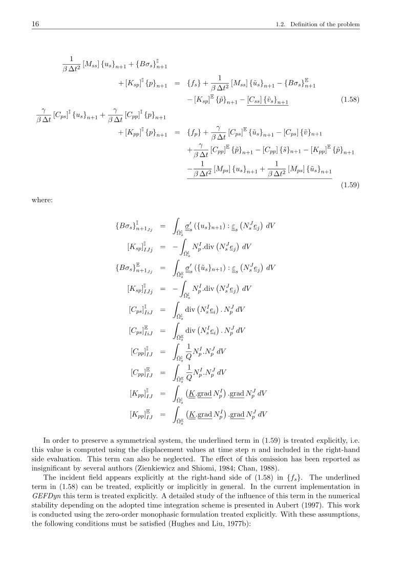
16 1.2. Definition of the problem
1
β∆t2[Mss] usn+1 + BσsIn+1
+ [Ksp]I pn+1 = fs+
1
β∆t2[Mss] usn+1 − BσsEn+1
− [Ksp]E pn+1 − [Css] vsn+1 (1.58)
γ
β∆t[Cps]
I usn+1 +γ
β∆t[Cpp]
I pn+1
+ [Kpp]I pn+1 = fp+
γ
β∆t[Cps]
E usn+1 − [Cps] vn+1
+γ
β∆t[Cpp]
E pn+1 − [Cpp] sn+1 − [Kpp]E pn+1
− 1
β∆t2[Mps] usn+1 +
1
β∆t2[Mps] usn+1
(1.59)
where:
BσsIn+1Jj=
∫
ΩIs
σ′s(usn+1) : ε
s
(NJs ej)dV
[Ksp]I
IJj= −
∫
ΩIs
N Ip .div
(NJs ej)dV
BσsEn+1Jj=
∫
ΩEs
σ′s(usn+1) : ε
s
(NJs ej)dV
[Ksp]I
IJj= −
∫
ΩIs
N Ip .div
(NJs ej)dV
[Cps]I
IiJ=
∫
ΩIs
div(N Is ei). NJ
p dV
[Cps]E
IiJ=
∫
ΩEs
div(N Is ei). NJ
p dV
[Cpp]I
IJ=
∫
ΩIs
1
QN Ip .N
Jp dV
[Cpp]E
IJ=
∫
ΩEs
1
QN Ip .N
Jp dV
[Kpp]I
IJ=
∫
ΩIs
(K.gradN I
p
).gradNJ
p dV
[Kpp]E
IJ=
∫
ΩEs
(K.gradN I
p
).gradNJ
p dV
In order to preserve a symmetrical system, the underlined term in (1.59) is treated explicitly, i.e.this value is computed using the displacement values at time step n and included in the right-handside evaluation. This term can also be neglected. The effect of this omission has been reported asinsignificant by several authors (Zienkiewicz and Shiomi, 1984; Chan, 1988).
The incident field appears explicitly at the right-hand side of (1.58) in fs. The underlinedterm in (1.58) can be treated, explicitly or implicitly in general. In the current implementation inGEFDyn this term is treated explicitly. A detailed study of the influence of this term in the numericalstability depending on the adopted time integration scheme is presented in Aubert (1997). This workis conducted using the zero-order monophasic formulation treated explicitly. With these assumptions,the following conditions must be satisfied (Hughes and Liu, 1977b):

Chapter 1. Numerical modeling of non-linear dynamical SSI 17
γ ≥ 1
2
and if [M ] is defined as:
[M ] = [M ]E − ∆t
2[C]E − ∆t2γ
2[K]E
[M ] must be positive-definite, where [·]E denotes symbolically the system mass matrix, the systemstiffness matrix and the system damping matrix associated to explicitly treated element groups. Nev-ertheless, the convergence of the explicit elements must be treated case to case, and usually will controlthe maximum allowed time step ∆t for the global numerical stability.
The incident displacement and velocity field needed for computation are obtained by numericalintegration of the input accelerogram with respect to time. This integration requires initial values,which are often unknown, due to recording techniques. A bad initial information leads to a purelynumerical drift on displacements when the numerical simulations are carried out. In order to avoid thiskind of numerical effect, one of the various base-line correction techniques available in the literaturemust be used over the incident field.
1.2.7 Resolution of non-linear system
The system defined by the equations (1.57) and (1.59) is in general non-linear. Therefore, the resolu-tion of the implicit terms must be carried out using an iterative algorithm. The iterative procedureimplemented in GEFDyn is a variation of the method of Newton, using a linearized version of thenon-linear system. If the total DOFs of the model are regrouped into a single vector x, the entirenon-linear system for a time step n+ 1 can be written as:
G (xn+1) = R (xn+1) − F (xn+1) = 0 ; xn+1 =
ubn+1
usn+1
pn+1
(1.60)
where Rn+1 regroups the implicit terms and Fn+1 the explicit terms and the external loading.The strategy consists to replace Gn+1 for the current iteration k + 1 by its linearization aroundthe previous iteration k (xkn+1 is known) following the incremental direction δx. The truncatedTaylor’s series (first order) is:
G(
xk+1n+1
)
=
G(
xkn+1
)
+
[
∂Gkn+1
∂x
]
.(
xk+1n+1 − xkn+1
)
(1.61)
with the definition of the unknown vector:
δxk+1n+1 = xk+1
n+1 − xkn+1 (1.62)
The matrix
[∂Gk
n+1
∂x
]
corresponds to the tangent stiffness matrix [K]kn+1 for the iteration k and
load step (or time step) n+ 1. Assuming that the stiffness matrix is not singular, the equation (1.60)can be rewritten as:
δxk+1n+1 =
(
[K]kn+1
)−1 (
Fn+1 − Rkn+1
)
(1.63)
The exact Jacobian matrix is used as stiffness matrix for the iterative procedure. The computedincremental correction δxk+1
n+1 is used to evaluate the new approximation of displacements and pres-sures:
xk+1n+1 = xkn+1 + δxk+1
n+1 (1.64)
18 1.3. Non-linear constitutive models
The total time consumption for a complete analysis is strongly dependent on the constructionand factorization of the Jacobian matrix. The classic implementation of Newton method updates thetangent stiffness matrix at each iteration, but for large systems this strategy can be excessively timeconsuming. The modified Newton method keeps the initial tangent matrix [K]0 during the completeanalysis. This strategy can increase significantly the number of iterations required to attempt theconvergence. The strategy adopted in GEFDyn is allows the user to select the number of loading steps(or time steps) during which the tangent stiffness matrix is kept, then:
[K]q .∂xk+1n+1 = Fn+1 − Rkn+1 with q < n+ 1 (1.65)
Additionally, the coefficients of the matrix [K]q can be given by the user (auxiliary stiffness values),
in order to improve the converge. The detailed expressions of Fn+1 and Rkn+1 can be derivedstraightforward combining the incremental form of the unknowns for the time step n+ 1 at iterationk + 1:
δubk+1n+1 = ubk+1
n+1 − ubkn+1
δusk+1n+1 = usk+1
n+1 − uskn+1
δpk+1n+1 = pk+1
n+1 − pkn+1
δubn+1 = ubn+1 − ubkn+1
δusn+1 = usn+1 − uskn+1
δpn+1 = pn+1 − pkn+1 (1.66)
with the equations (1.57) and (1.59). Concerning the convergence, the iterative procedure stops whenthe relative norms of the displacements u, pressures p and the corresponding unbalanced forcesor right-hand side values of (1.60) G (u) and G (p) reach a defined tolerance value (utol, ptol,Rutol and Rptol ):
‖uk+1n+1 − ukn+1‖
‖uk+1n+1 − un‖
< utol
‖pk+1n+1 − pkn+1‖
‖pk+1n+1 − pn‖
< ptol
‖ G (u)k+1n+1‖
‖ G (u)0n+1‖< Rutol
‖ G (p)k+1n+1‖
‖ G (p)0n+1‖< Rptol (1.67)
where the norm is defined by:
‖a‖ =√
at.aUsually, tolerance values near to 10−3 for displacements and pressures, and 10−2 for the right-hand
side terms give satisfactory results.
1.3 Non-linear constitutive models
The main sources of non-linearities in an earthquake SSI problem are related to material behaviorand second order geometrical effects, for instance P − ∆ effects of the superstructure. This work isfocused on the role of non-linear behavior of the soil and its effect on the non-linear dynamical soil-structure interaction. According with this purpose, geometrical non-linearities are neglected and the
Chapter 1. Numerical modeling of non-linear dynamical SSI 19
small-strain assumption is kept for the formulation of the non-linear behavior of each component ofthe complete model. The next sections describe the main aspects of each used non-linear constitutivemodel for the soil, the interface and the superstructure.
1.3.1 Mechanical interfaces
The contact problem between the soil and the foundation was treated by interface elements. Theoriginal formulation proposed by Aubry et al. (1990) was adapted for this work, using the same generalhypothesis and making the necessary modifications to integrate an initial thickness. Additionally,the numeric integration quadrature was modified from Gauss to Newton-Cotes, in order to reducenumber of iterations. This numerical integration approach introduces a lumped stiffness matrix forthe interface, reducing the interaction with the opening or closing state of neighboring elements. As thesuperstructure domain Ωb is assumed to be monophasic, the used interface model is purely mechanicimposing a null normal flux from the soil domain Ωs. Details regarding the formulation, numericalintegration and model parameters are given in Appendix B.
The main purpose of introducing joint elements in this work is to improve the numerical treatmentof the stress concentration zone between the foundation and the soil, i.e. prevent the apparition oftraction in the soil. In fact, the stress concentration at the corners of the foundation can be reducedallowing the sliding between the two solids. The problem of the uplift during the dynamic loadingappears usually for tall and slender structures, such as bridge piers, antennas or elevated water tanks.As the focus of this work is the role of non-linear soil behavior in the dynamic response of mediumregular buildings, the set of parameters for the joint elements is selected in order to obtain sliding butnot uplift.
1.3.2 Continuous non-linear beam model
According to kinematic assumption presented in §1.2, the superstructure domain Ωb is modeled byBernouilli beams. The main assumption is related to the thinness of the beam element (transversesection size compared to beam length) which allows to consider these elements as lines rather thanvolumes.
The first version of continuous Bernoulli beam was developed and included by Aubry and Modaressi(1996) in GEFDyn on the basis of the implementation proposed by Bathe (1996) for general curvedbeam elements. Later, Pianka (1998) extends the formulation to thick beams. In this work, thefirst formulation was used with some modifications and improvements concerning the consistent massmatrix computation, the internal forces calculation and the integration of the constitutive model.Details about the formulation and numerical integration of the used constitutive model are given inAppendix C.
The integrals defining mass and stiffness matrices and body and external forces, are computednumerically using a Newton-Cotes quadrature. The implementation in GEFDyn allows to choosedifferent order of integration following each local axis of the element r, s and t (Fig.1.2). When a non-linear constitutive model is used, the order of integration must be high enough to assess the evolutionof the plastic zone during the load. For earthquake loading, the plastic zones are concentrated atthe ends of beams and columns, i.e. an elevated order of integration (over the spam and the flexuraldirection) is required in these zones. A low order of integration can be used for mid spam elements orfor foundation beams.
1.3.3 Plastic hinges beam model
As previously noted, during an earthquake loading the nonlinearities of structural elements are con-centrated near to ends of horizontal spam or extreme section of the columns. The beam elementdeveloped in the previous section integrates a constitutive model across the entire element, i.e. oversome sections that remain essentially elastic during the dynamic response. The non-linear behavioris expressed in terms of a strain-stress constitutive model, that is a suitable approach for example
20 1.3. Non-linear constitutive models
for steel structural elements. For reinforced concrete elements, this kind of approach is complex andrequires the definition of multi-fiber elements, including constitutive relation for concrete and steelfibers that are integrated simultaneously using appropriate compatibility relations. As the emphasis ofthis work is on the non-linear soil behavior, a more global approach is desirable to asses the non-linearbehavior of reinforced-concrete structural elements. According to this purpose, a concentrated plastichinge beam-column element has been introduced in GEFDyn during this work (Saez, 2007).
The beam model added to GEFDyn has nonlinear hysteretic bending moment-end rotation char-acteristics. The model is based on the two-component model presented by Giberson (1969) and themodifications included in DRAIN-2DX (Prakash et al., 1993) and PC-ANSR (Maison, 1992) softwaresto take into account axial force and bending moment interaction. The basic DRAIN-2DX (2D) andPC-ANSR (3D) model was extended to some features of GEFDyn : elementary body forces, consistentand lumped elementary mass, sequential construction availability, etc. Details about the model areprovided in Appendix D.
1.3.4 Constitutive modeling of the soil
The ECP elastoplastic multi-mechanism model (Aubry et al., 1982; Hujeux, 1985), commonly calledHujeux model is used to represent the soil behavior. This model can take into account the soil behaviorin a large range of deformations. The model is written in terms of effective stress. The representation ofall irreversible phenomena is made by four coupled elementary plastic mechanisms: three plane-straindeviatoric plastic deformation mechanisms in three orthogonal planes and an isotropic one. The modeluses a Coulomb type failure criterion and the critical state concept. The evolution of hardening is basedon the plastic strain (deviatoric and volumetric strain for the deviatoric mechanisms and volumetricstrain for the isotropic one). To take into account the cyclic behavior a kinematical hardening basedon the state variables at the last load reversal is used. The soil behavior is decomposed into elastic,pseudo-elastic, hysteretic and mobilized domains. In the Appendix E, the ECP elastoplastic multi-mechanism model in its generic formulation is presented. A general description of the numericalintegration procedure is also provided in this Appendix.
In a general way, the number of parameters of a constitutive model is related to the number ofphysical phenomena described by the model. Thus, for a very complex material behavior such as thesoil, we must accept an elevated number of parameters. In a practical point of view, we need to be ableto identify the model parameters in a simple way adapted to standard available data. According tothis goal, several works have been conducted at ECP in order to define sets of parameters for diversematerials under different loading paths for the different versions of multimechanism model. Theseparameters collections have been tested and validated in order to verify the performance in modelingrealistic soil behavior.
The numerical simulation of laboratory tests has been extensively studied by Hujeux (1979), Hajal(1984), Rahma (1988), Michalski and Rahma (1989), Piccuezzu (1991), Hicher and Rahma (1994),Michali (1994), Kordjani (1995) and Modaressi and Lopez-Caballero (2001), among others. Studies onthe accuracy of the model in applications related to earthquake engineering have been carried out byHujeux (1985), Modaressi (1987), Aubry and Modaressi (1989), Modaressi and Aubry (1989), Aubryand Modaressi (1992b), Benzenatti (1992), Modaressi et al. (1995), Mellal (1997), Sica (2001) andLopez-Caballero and Modaressi (2002) among others. Other than Hujeux (1985) and Kordjani (1995),the major part of these studies were oriented to monotonic loading. Recently, Lopez-Caballero (2003)and Modaressi (2003) presented a strategy for parameters identification oriented to cyclic behavior.
A particular aspect of the multimechanism model presented in Appendix E is that it was writtenfor a large range of deformation. According to this, even if laboratory data is available, there arepractical difficulties to explode these results for very large deformation (near to critical state) or forvery small deformations (elastic range). In order to encompass these difficulties, the strategy proposedby Lopez-Caballero and Modaressi-Farahmand Razavi (2008) takes into account several results ofdifferent studies that highlight correlations between intrinsic characteristics of the soils (e.g. elasticmodulus or critical states parameters) to well-known properties traditionally used in soil mechanics
Chapter 1. Numerical modeling of non-linear dynamical SSI 21
(e.g. Atterberg’s limits or granulometry properties). These correlations and considerations on therepresentation of physical aspects of the soil by the constitutive model are combined with severalreference curves in order to define a practical strategy to set-up the model parameters.
Concerning the identification of parameters for cyclic loading, the proposed strategy is based onthe numerical simulation of laboratory tests with special emphasis on modulus degradation G− γ anddamping D − γ curves. The goal is to identify a set of parameters using a minimum of laboratorydata and a maximum of information available from correlations. According with this purpose, a firstparameter classification can be done in terms of the role of each parameter in the model: Elasticity: K, G, p′ref and ne Plasticity and critical state: φ′pp, β, b and d Hardening: ψ, a1, a2, np and c Threshold domain: relk , rhysk , rmobk and reliso Initial state: pc0
Table 1.1: Classification of the Elastoplastic model parameters
Stiffness State Hardening
Directlymeasured
G, K and β φ′pp, ψ and d
Non-Directlymeasured
a1 and a2 brelak , rhysk ,rmobk , np, c,reliso and c
Concerning the role of each parameter related to soil behavior, the parameters can be separatedinto three categories: parameters related to the stiffness (strain-stress relation), those associated to thestate independent of the loading history (e.g. φ′pp or b) and those related to the evolution of hardeningvariables. Finally, the strategy proposed by Lopez-Caballero and Modaressi-Farahmand Razavi (2008)proposes a separation related to the estimation method: those that can be directly measured fromeither in-situ or laboratory test results as elastic or perfect plasticity parameters, and those whichcannot be directly measured (Table 1.1). The initial state parameter pc0 is directly measurable. Thereader is addressed to references for further details concerning the parameter identification strategy.The numerical used values for each soil are given in the Appendix H. This appendix shows severalsoil mechanics test simulations used to verify the accuracy of each parameter set.
1.3.5 General remarks
The general monophasic and/or two phase dynamic formulation, some specific elements and the con-stitutive models used for the numerical modeling of the dynamical SSI problem were presented in theprevious sections and annexes. The GEFDyn code was enhanced by adding a new plastic-hinge beamcolumn element model. Other improvements have been done concerning the numerical integration ofinterface elements and the dynamic formulation of continuous beam elements. A specific formulationfor the modeling of dynamical SSI problem for regular buildings by a modified plane-strain approach ispresented in Chapter 3. A large amount of work has been devoted to develop pre and post-treatmenttools required to perform numerically-costly applications presented in next chapters. In this way, sev-eral improvements in run time and numerical capacity of GEFDyn have been performed during thiswork.

22 1.4. Special aspects of the numerical resolution of the dynamic SSI problem with Finite Elements
Next section is devoted to some specific aspects of the numerical modelization of dynamical SSIconcerning damping considerations and the treatment of the boundary conditions under dynamicalloading for the non-linear behavior case. With this purpose, some theoretical and numerical validationsare presented.
1.4 Special aspects of the numerical resolution of the dynamic SSIproblem with Finite Elements
As previously discussed in §1.2.3, when the dynamic SSI problem is treated by finite elements somespecial considerations must be included in order to ensure that the truncated domain model be com-patible with the unbounded nature of the real problem. If the soil remains elastic under dynamicloading, the use of absorbing elements such as paraxial elements described in Appendix A provides arelative simple way to modeling the unbounded soil domain. Even if several other forms of radiationboundary conditions have been developed last years as discussed by Wolf and Song (1996), or morerecently by Basu and Chopra (2003), these forms are suitable only for linear elastic materials. As thescope of this work is the non-linear material behavior, a tied lateral boundary approach (Zienkiewiczet al., 1988, 1999) or repeatable approach is retained as modeling strategy (Fig.1.4).
b
repeatabilityspacing
tied lateralboundaries
incoming motion andabsorbing boundary
Figure 1.4: Tied lateral boundary approach
In a general way, if we consider a horizontally stratified soil with an incoming seismic input prop-agating following the vertical direction, a superstructure can be interpreted as a perturbation to theone-dimensional wave propagation problem. Due to this perturbation, the waves are reflected not onlyin the vertical direction. Assuming that the model truncation is deep enough to verify elastic behaviorat the bottom, the last can be treated by previously described paraxial approximation. Thus, theonly additional problem arises from the appropriate treatment of the vertical lateral boundaries. Inthese boundaries, it is necessary to allow the radiation of the waves caused by the superstructure.These radiated waves can be expressed in terms of the difference between the free field solution (i.e.the solution of the one-dimensional wave propagation problem) and the total field associated to thesoil-structure problem. Zienkiewicz et al. (1988) propose to write the equilibrium equations in termsof the relative displacements to the incoming displacement field at the bottom truncation level andadd a fictitious transmitting layer interpreted as the last layer of elements along the lateral boundariesof the mesh. These transmitting layers are used to transmit the perturbed motion caused by thesuperstructure. The numerical procedure involves the parallel resolution of the main mesh and theone-dimensional column, the resolution of the transmitting layer and the application of the obtaineddifference field as nodal prescribed displacements to main mesh. Additionally, this approach requiresthat the region near to truncation lateral boundary remains elastic and homogenous under the loading.
A simpler alternative to the treatment suggested by Zienkiewicz et al. (1988) is the tied lateralboundary approach or repeatable boundary conditions which is illustrated in Fig.1.4. In this approach,the periodic nature of the surface perturbation is assumed, thus a sequence of superstructures is placed
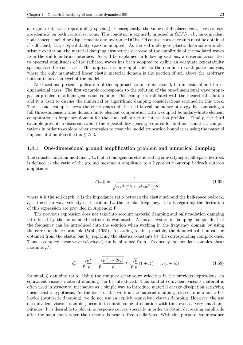
Chapter 1. Numerical modeling of non-linear dynamical SSI 23
at regular intervals (repeatability spacing). Consequently, the values of displacements, stresses, etc.are identical on both vertical sections. This condition is explicitly imposed in GEFDyn by an equivalentnode concept including displacements and hydraulic DOFs. Of course, correct results must be obtainedif sufficiently large repeatability space is adopted. As the soil undergoes plastic deformation underseismic excitation, the material damping ensures the decrease of the amplitude of the radiated wavesfrom the soil-foundation interface. As will be explained in following sections, a criterion associatedto spectral amplitudes of the radiated waves has been adopted to define an adequate repeatabilityspacing case for each case. This approach is fully applicable to the non-linear earthquake analysis,where the only maintained linear elastic material domain is the portion of soil above the arbitrarybottom truncation level of the model.
Next sections present application of this approach to one-dimensional, bi-dimensional and three-dimensional cases. The first example corresponds to the solution of the one-dimensional wave propa-gation problem of a homogenous soil column. This example is validated with the theoretical solutionand it is used to discuss the numerical or algorithmic damping considerations retained in this work.The second example shows the effectiveness of the tied lateral boundary strategy by comparing afull three-dimension time domain finite element computation with a coupled boundary-finite elementcomputation in frequency domain for the same soil-structure interaction problem. Finally, the thirdexample presents a discussion about the repeatability spacing required for bi-dimensional FE compu-tations in order to explore other strategies to treat the model truncation boundaries using the paraxialimplementation described in §1.2.3.
1.4.1 One-dimensional ground amplification problem and numerical damping
The transfer function modulus |T (ω)| of a homogenous elastic soil layer overlying a half-space bedrockis defined as the ratio of the ground movement amplitude to a hypothetic outcrop bedrock outcropamplitude:
|T (ω)| = 1√
cos2 iωcsh+ α2 sin2 iω
csh
(1.68)
where h is the soil depth, α is the impedance ratio between the elastic soil and the half-space bedrock,cs is the shear wave velocity of the soil and ω the circular frequency. Details regarding the derivationof this expression are provided in Appendix F.
The previous expression does not take into account material damping and only radiation dampingintroduced by the unbounded bedrock is evaluated. A linear hysteretic damping independent ofthe frequency can be introduced into the solution when working in the frequency domain by usingthe correspondence principle (Wolf, 1985). According to this principle, the damped solution can beobtained from the elastic one by replacing the elastics constants by the corresponding complex ones.Thus, a complex shear wave velocity c∗s can be obtained from a frequency-independent complex shearmodulus µ∗:
c∗s =
√µ∗
ρ=
√
µ (1 + 2iζ)
ρ≈√µ
ρ(1 + iζ) = cs (1 + iζ) (1.69)
for small ζ damping ratio. Using the complex shear wave velocities in the previous expressions, anequivalent viscous material damping can be introduced. This kind of equivalent viscous material isoften used in structural mechanics as a simple way to introduce material energy dissipation satisfyinglinear elastic hypothesis. As the focus of this work is the material damping related to non-linear be-havior (hysteretic damping), we do not use an explicit equivalent viscous damping. However, the useof equivalent viscous damping permits to obtain some attenuation with time even at very small am-plitudes. It is desirable to plot time response curves, specially in order to obtain decreasing amplitudeafter the main shock when the response is near to free-oscillations. With this purpose, we introduce
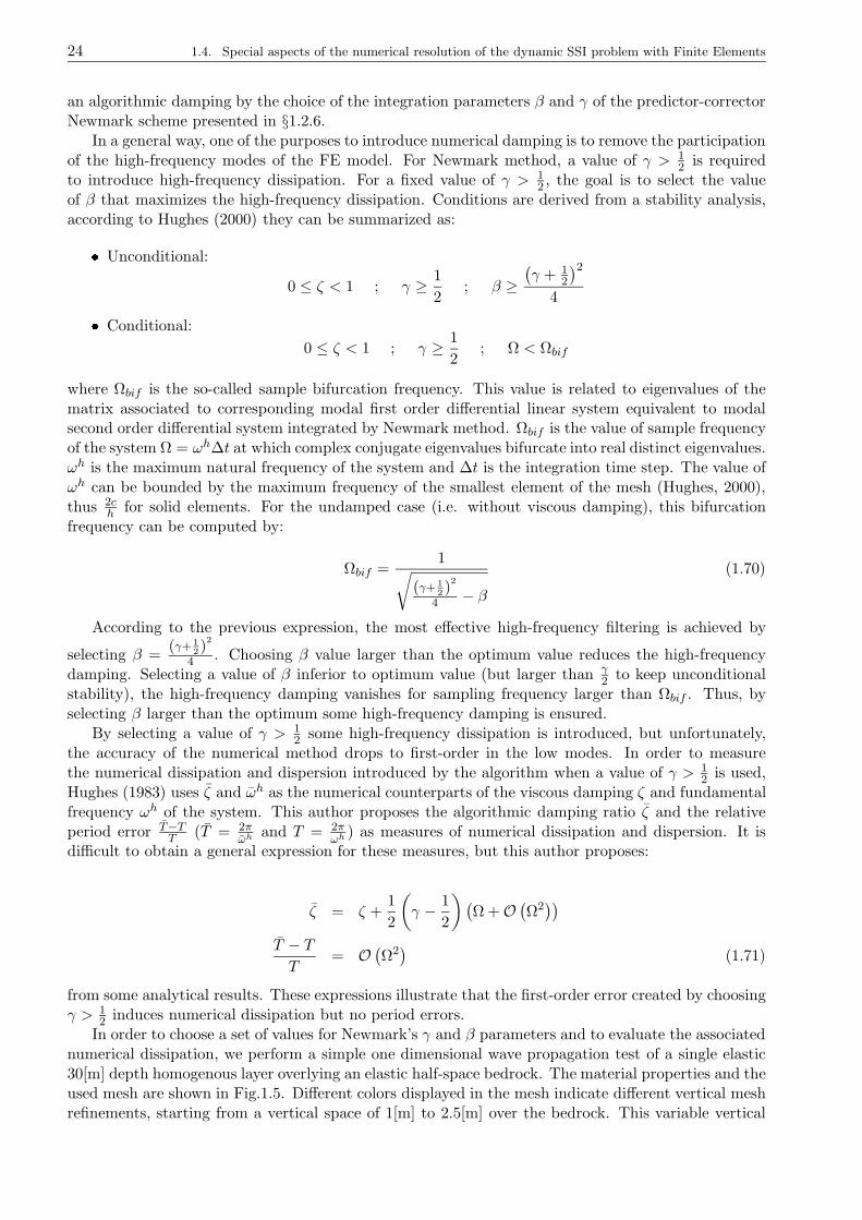
24 1.4. Special aspects of the numerical resolution of the dynamic SSI problem with Finite Elements
an algorithmic damping by the choice of the integration parameters β and γ of the predictor-correctorNewmark scheme presented in §1.2.6.
In a general way, one of the purposes to introduce numerical damping is to remove the participationof the high-frequency modes of the FE model. For Newmark method, a value of γ > 1
2 is requiredto introduce high-frequency dissipation. For a fixed value of γ > 1
2 , the goal is to select the valueof β that maximizes the high-frequency dissipation. Conditions are derived from a stability analysis,according to Hughes (2000) they can be summarized as: Unconditional:
0 ≤ ζ < 1 ; γ ≥ 1
2; β ≥
(γ + 1
2
)2
4 Conditional:
0 ≤ ζ < 1 ; γ ≥ 1
2; Ω < Ωbif
where Ωbif is the so-called sample bifurcation frequency. This value is related to eigenvalues of thematrix associated to corresponding modal first order differential linear system equivalent to modalsecond order differential system integrated by Newmark method. Ωbif is the value of sample frequencyof the system Ω = ωh∆t at which complex conjugate eigenvalues bifurcate into real distinct eigenvalues.ωh is the maximum natural frequency of the system and ∆t is the integration time step. The value ofωh can be bounded by the maximum frequency of the smallest element of the mesh (Hughes, 2000),thus 2c
hfor solid elements. For the undamped case (i.e. without viscous damping), this bifurcation
frequency can be computed by:
Ωbif =1
√
(γ+ 12)
2
4 − β(1.70)
According to the previous expression, the most effective high-frequency filtering is achieved by
selecting β =(γ+ 1
2)2
4 . Choosing β value larger than the optimum value reduces the high-frequencydamping. Selecting a value of β inferior to optimum value (but larger than γ
2 to keep unconditionalstability), the high-frequency damping vanishes for sampling frequency larger than Ωbif . Thus, byselecting β larger than the optimum some high-frequency damping is ensured.
By selecting a value of γ > 12 some high-frequency dissipation is introduced, but unfortunately,
the accuracy of the numerical method drops to first-order in the low modes. In order to measurethe numerical dissipation and dispersion introduced by the algorithm when a value of γ > 1
2 is used,Hughes (1983) uses ζ and ωh as the numerical counterparts of the viscous damping ζ and fundamentalfrequency ωh of the system. This author proposes the algorithmic damping ratio ζ and the relativeperiod error T−T
T(T = 2π
ωh and T = 2πωh ) as measures of numerical dissipation and dispersion. It is
difficult to obtain a general expression for these measures, but this author proposes:
ζ = ζ +1
2
(
γ − 1
2
)(Ω +O
(Ω2))
T − TT
= O(Ω2)
(1.71)
from some analytical results. These expressions illustrate that the first-order error created by choosingγ > 1
2 induces numerical dissipation but no period errors.In order to choose a set of values for Newmark’s γ and β parameters and to evaluate the associated
numerical dissipation, we perform a simple one dimensional wave propagation test of a single elastic30[m] depth homogenous layer overlying an elastic half-space bedrock. The material properties and theused mesh are shown in Fig.1.5. Different colors displayed in the mesh indicate different vertical meshrefinements, starting from a vertical space of 1[m] to 2.5[m] over the bedrock. This variable vertical
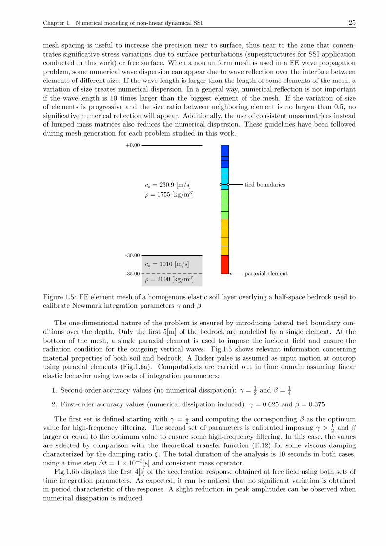
Chapter 1. Numerical modeling of non-linear dynamical SSI 25
mesh spacing is useful to increase the precision near to surface, thus near to the zone that concen-trates significative stress variations due to surface perturbations (superstructures for SSI applicationconducted in this work) or free surface. When a non uniform mesh is used in a FE wave propagationproblem, some numerical wave dispersion can appear due to wave reflection over the interface betweenelements of different size. If the wave-length is larger than the length of some elements of the mesh, avariation of size creates numerical dispersion. In a general way, numerical reflection is not importantif the wave-length is 10 times larger than the biggest element of the mesh. If the variation of sizeof elements is progressive and the size ratio between neighboring element is no largen than 0.5, nosignificative numerical reflection will appear. Additionally, the use of consistent mass matrices insteadof lumped mass matrices also reduces the numerical dispersion. These guidelines have been followedduring mesh generation for each problem studied in this work.
+0.00
-30.00
-35.00
cs = 230.9 [m/s]
cs = 1010 [m/s]
ρ = 1755 [kg/m3]
ρ = 2000 [kg/m3]
tied boundaries
paraxial element
Figure 1.5: FE element mesh of a homogenous elastic soil layer overlying a half-space bedrock used tocalibrate Newmark integration parameters γ and β
The one-dimensional nature of the problem is ensured by introducing lateral tied boundary con-ditions over the depth. Only the first 5[m] of the bedrock are modelled by a single element. At thebottom of the mesh, a single paraxial element is used to impose the incident field and ensure theradiation condition for the outgoing vertical waves. Fig.1.5 shows relevant information concerningmaterial properties of both soil and bedrock. A Ricker pulse is assumed as input motion at outcropusing paraxial elements (Fig.1.6a). Computations are carried out in time domain assuming linearelastic behavior using two sets of integration parameters:
1. Second-order accuracy values (no numerical dissipation): γ = 12 and β = 1
4
2. First-order accuracy values (numerical dissipation induced): γ = 0.625 and β = 0.375
The first set is defined starting with γ = 12 and computing the corresponding β as the optimum
value for high-frequency filtering. The second set of parameters is calibrated imposing γ > 12 and β
larger or equal to the optimum value to ensure some high-frequency filtering. In this case, the valuesare selected by comparison with the theoretical transfer function (F.12) for some viscous dampingcharacterized by the damping ratio ζ. The total duration of the analysis is 10 seconds in both cases,using a time step ∆t = 1× 10⁻³[s] and consistent mass operator.
Fig.1.6b displays the first 4[s] of the acceleration response obtained at free field using both sets oftime integration parameters. As expected, it can be noticed that no significant variation is obtainedin period characteristic of the response. A slight reduction in peak amplitudes can be observed whennumerical dissipation is induced.
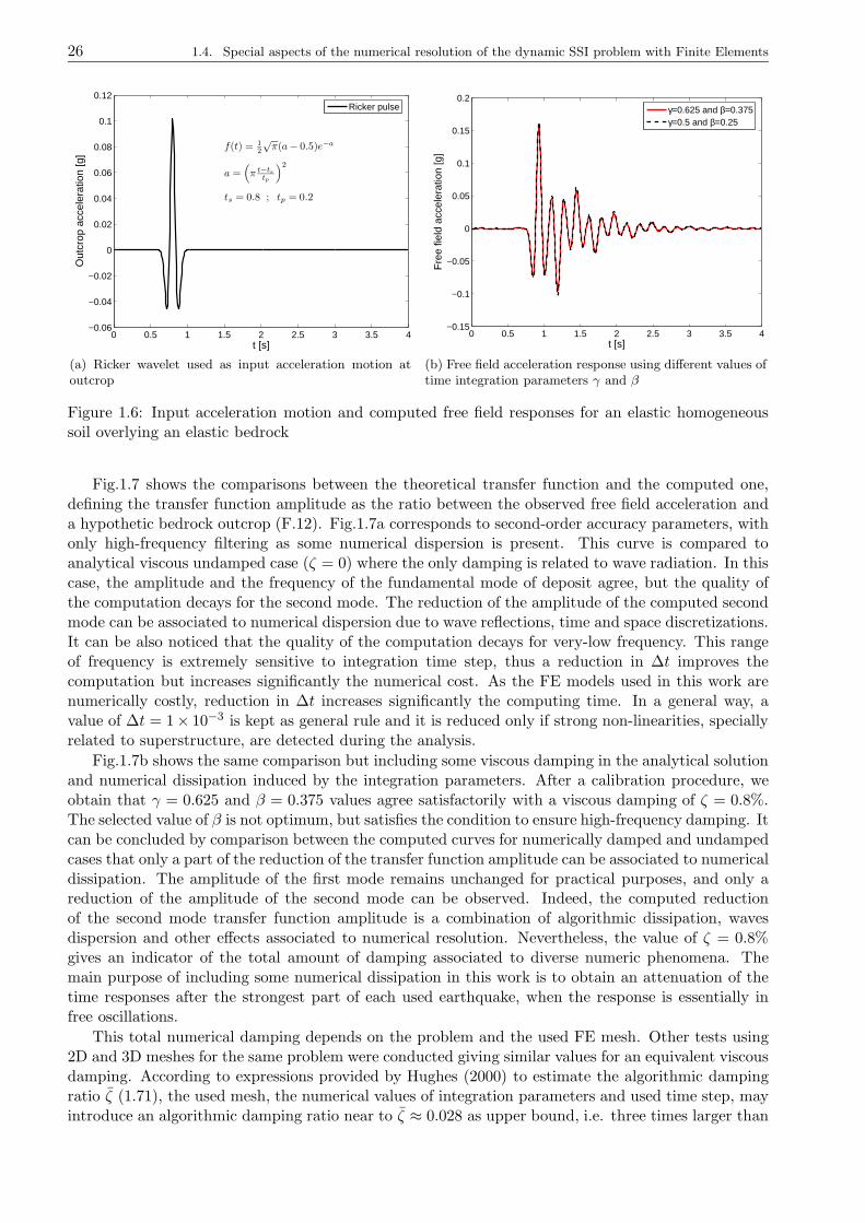
26 1.4. Special aspects of the numerical resolution of the dynamic SSI problem with Finite Elements
0 0.5 1 1.5 2 2.5 3 3.5 4−0.06
−0.04
−0.02
0
0.02
0.04
0.06
0.08
0.1
0.12
t [s]
Out
crop
acc
eler
atio
n [g
]
f(t) = 1
2
√π(a− 0.5)e−a
a =(
π t−ts
tp
)2
ts = 0.8 ; tp = 0.2
Ricker pulse
(a) Ricker wavelet used as input acceleration motion atoutcrop
0 0.5 1 1.5 2 2.5 3 3.5 4−0.15
−0.1
−0.05
0
0.05
0.1
0.15
0.2
t [s]
Fre
e fie
ld a
ccel
erat
ion
[g]
γ=0.625 and β=0.375γ=0.5 and β=0.25
(b) Free field acceleration response using different values oftime integration parameters γ and β
Figure 1.6: Input acceleration motion and computed free field responses for an elastic homogeneoussoil overlying an elastic bedrock
Fig.1.7 shows the comparisons between the theoretical transfer function and the computed one,defining the transfer function amplitude as the ratio between the observed free field acceleration anda hypothetic bedrock outcrop (F.12). Fig.1.7a corresponds to second-order accuracy parameters, withonly high-frequency filtering as some numerical dispersion is present. This curve is compared toanalytical viscous undamped case (ζ = 0) where the only damping is related to wave radiation. In thiscase, the amplitude and the frequency of the fundamental mode of deposit agree, but the quality ofthe computation decays for the second mode. The reduction of the amplitude of the computed secondmode can be associated to numerical dispersion due to wave reflections, time and space discretizations.It can be also noticed that the quality of the computation decays for very-low frequency. This rangeof frequency is extremely sensitive to integration time step, thus a reduction in ∆t improves thecomputation but increases significantly the numerical cost. As the FE models used in this work arenumerically costly, reduction in ∆t increases significantly the computing time. In a general way, avalue of ∆t = 1× 10⁻³ is kept as general rule and it is reduced only if strong non-linearities, speciallyrelated to superstructure, are detected during the analysis.
Fig.1.7b shows the same comparison but including some viscous damping in the analytical solutionand numerical dissipation induced by the integration parameters. After a calibration procedure, weobtain that γ = 0.625 and β = 0.375 values agree satisfactorily with a viscous damping of ζ = 0.8%.The selected value of β is not optimum, but satisfies the condition to ensure high-frequency damping. Itcan be concluded by comparison between the computed curves for numerically damped and undampedcases that only a part of the reduction of the transfer function amplitude can be associated to numericaldissipation. The amplitude of the first mode remains unchanged for practical purposes, and only areduction of the amplitude of the second mode can be observed. Indeed, the computed reductionof the second mode transfer function amplitude is a combination of algorithmic dissipation, wavesdispersion and other effects associated to numerical resolution. Nevertheless, the value of ζ = 0.8%gives an indicator of the total amount of damping associated to diverse numeric phenomena. Themain purpose of including some numerical dissipation in this work is to obtain an attenuation of thetime responses after the strongest part of each used earthquake, when the response is essentially infree oscillations.
This total numerical damping depends on the problem and the used FE mesh. Other tests using2D and 3D meshes for the same problem were conducted giving similar values for an equivalent viscousdamping. According to expressions provided by Hughes (2000) to estimate the algorithmic dampingratio ζ (1.71), the used mesh, the numerical values of integration parameters and used time step, mayintroduce an algorithmic damping ratio near to ζ ≈ 0.028 as upper bound, i.e. three times larger than
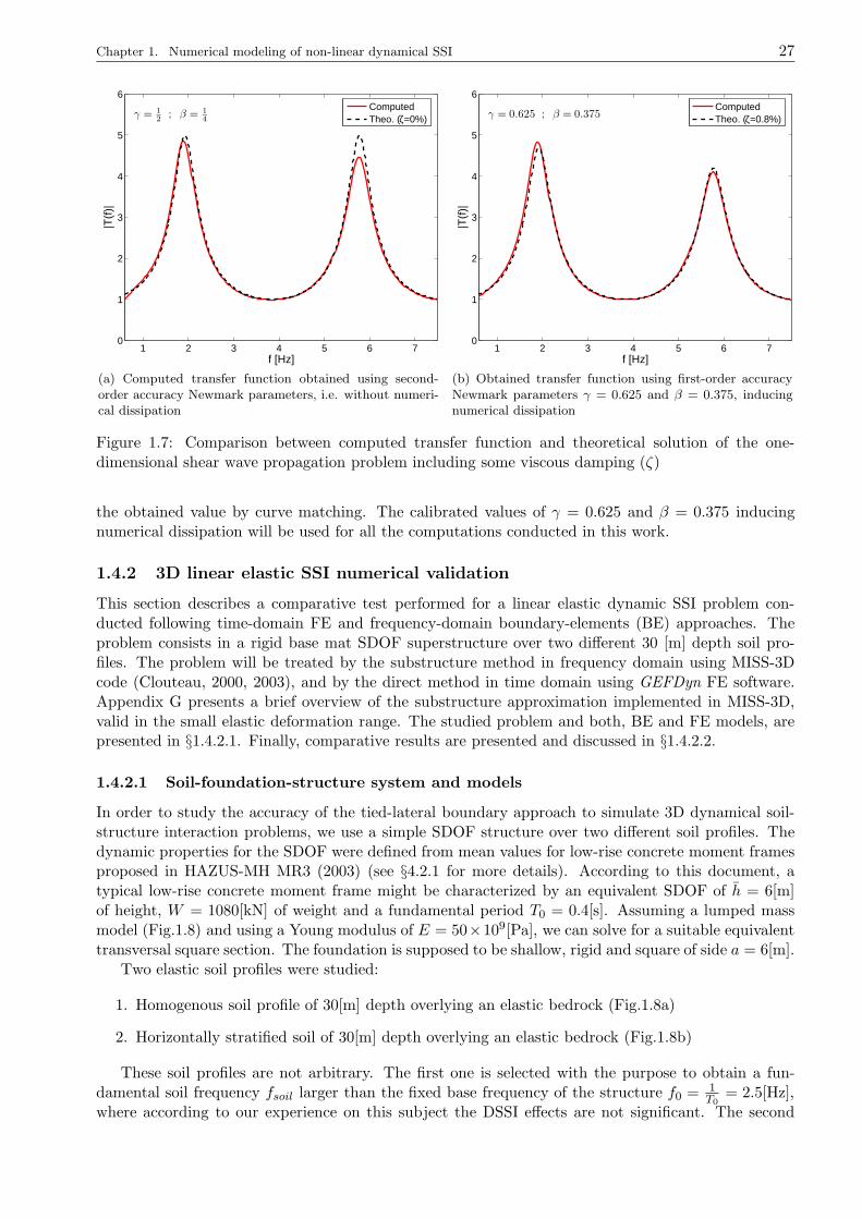
Chapter 1. Numerical modeling of non-linear dynamical SSI 27
1 2 3 4 5 6 70
1
2
3
4
5
6
f [Hz]
|T(f
)|γ = 1
2; β = 1
4
ComputedTheo. (ζ=0%)
(a) Computed transfer function obtained using second-order accuracy Newmark parameters, i.e. without numeri-cal dissipation
1 2 3 4 5 6 70
1
2
3
4
5
6
f [Hz]
|T(f
)|
γ = 0.625 ; β = 0.375ComputedTheo. (ζ=0.8%)
(b) Obtained transfer function using first-order accuracyNewmark parameters γ = 0.625 and β = 0.375, inducingnumerical dissipation
Figure 1.7: Comparison between computed transfer function and theoretical solution of the one-dimensional shear wave propagation problem including some viscous damping (ζ)
the obtained value by curve matching. The calibrated values of γ = 0.625 and β = 0.375 inducingnumerical dissipation will be used for all the computations conducted in this work.
1.4.2 3D linear elastic SSI numerical validation
This section describes a comparative test performed for a linear elastic dynamic SSI problem con-ducted following time-domain FE and frequency-domain boundary-elements (BE) approaches. Theproblem consists in a rigid base mat SDOF superstructure over two different 30 [m] depth soil pro-files. The problem will be treated by the substructure method in frequency domain using MISS-3Dcode (Clouteau, 2000, 2003), and by the direct method in time domain using GEFDyn FE software.Appendix G presents a brief overview of the substructure approximation implemented in MISS-3D,valid in the small elastic deformation range. The studied problem and both, BE and FE models, arepresented in §1.4.2.1. Finally, comparative results are presented and discussed in §1.4.2.2.
1.4.2.1 Soil-foundation-structure system and models
In order to study the accuracy of the tied-lateral boundary approach to simulate 3D dynamical soil-structure interaction problems, we use a simple SDOF structure over two different soil profiles. Thedynamic properties for the SDOF were defined from mean values for low-rise concrete moment framesproposed in HAZUS-MH MR3 (2003) (see §4.2.1 for more details). According to this document, atypical low-rise concrete moment frame might be characterized by an equivalent SDOF of h = 6[m]of height, W = 1080[kN] of weight and a fundamental period T0 = 0.4[s]. Assuming a lumped massmodel (Fig.1.8) and using a Young modulus of E = 50×109[Pa], we can solve for a suitable equivalenttransversal square section. The foundation is supposed to be shallow, rigid and square of side a = 6[m].
Two elastic soil profiles were studied:
1. Homogenous soil profile of 30[m] depth overlying an elastic bedrock (Fig.1.8a)
2. Horizontally stratified soil of 30[m] depth overlying an elastic bedrock (Fig.1.8b)
These soil profiles are not arbitrary. The first one is selected with the purpose to obtain a fun-damental soil frequency fsoil larger than the fixed base frequency of the structure f0 = 1
T0= 2.5[Hz],
where according to our experience on this subject the DSSI effects are not significant. The second

28 1.4. Special aspects of the numerical resolution of the dynamic SSI problem with Finite Elements
+0.00
-30.00
Vs = 355 [m/s]
Vs = 1078 [m/s]
ρ = 1755 [kg/m3]
ρ = 2000 [kg/m3]
h
bm
a
(a) Homogenous soil profile
+0.00
-6.00
-12.00
-20.00
-30.00
Vs = 160 [m/s]
Vs = 225 [m/s]
Vs = 254 [m/s]
Vs = 275 [m/s]
Vs = 1078 [m/s]
b
(b) Horizontally stratified soil profile
Figure 1.8: Schema of both soil-structure systems used for the linear elastic comparative analysis
profile corresponds to a simplification of a homogenous dry sand profile studied in chapters 2 and 3.As it is explained in these chapters, when non-linear soil behavior is taken into account the initial stateof soil confinement is a key issue. The variation of initial confinement with effective vertical stress ismodeled by a non-linear elastic approach (E.4) in the multimechanism model. This vertical variationproduces a gradually increasing shear wave velocity profile with the depth. The soil profile in Fig.1.8bcorrespond to a discretization of this vertical variation, assuming constant shear wave velocity in eachlayer. In this case, the fundamental frequency of the soil fsoil is close to the fixed base frequency ofthe superstructure f0. In this condition, resonance phenomena between soil and structure producesignificative soil-structure interaction. Densities of the soil and the bedrock are the same for bothprofiles, they are omitted in Fig.1.8b for sake of simplicity.
Modeling assumptions and characteristics of each numerical model depends on the used codeand are detailed in the following. As MISS3D code requires linear elasticity, we used linear elasticconstitutive models for both soil and superstructure. We also impose that loss of contact betweensoil and foundation do not take place, thus we assume continuity of displacement and stress over thesoil-structure interface Σbs.
1.4.2.1.1 Substructure approach As mentioned in §G, in this approach the unbounded soilsubdomain is modeled with BEM and its response is disjointed from the solution of the superstructuralsubdomain. The superstructure is a FE model constructed using vertical beam elements and lumpingthe mass at 6[m] hight above the foundation level. The foundation is modeled using a regular mesh ofsolid 3D massless elements and imposing a kinematical constraint to ensure its rigidness. The surfacemeshes required for the boundary of the soil over the soil-structure interface is deduced from the finiteelement mesh of the superstructure. The coupling between FEM and BEM is conducted using a modalreduction technique. We use the Craig-Bampton reduction technique to export the FE superstructuremodel to MISS3D code accounting the six rigid body modes (3 translations and 3 rotations) and thefirst fixed base mode (Fig.1.9). We add a very stiff foundation beam following the load direction y, inorder to avoid relative rotation between column and foundation.
Concerning the damping, we use two different values: the first one ζ0 is related to the superstructureand the second one βs is assumed for the soil and the bedrock. The superstructure damping ratio ζ0
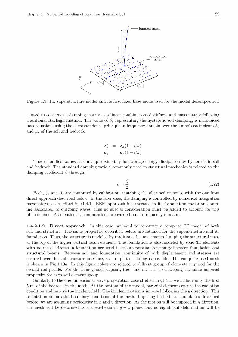
Chapter 1. Numerical modeling of non-linear dynamical SSI 29
z
x
y 6[m]6[m]
6[m
]
lumped mass
foundationbeam
Figure 1.9: FE superstructure model and its first fixed base mode used for the modal decomposition
is used to construct a damping matrix as a linear combination of stiffness and mass matrix followingtraditional Rayleigh method. The value of βs representing the hysteretic soil damping, is introducedinto equations using the correspondence principle in frequency domain over the Lame’s coefficients λsand µs of the soil and bedrock:
λ∗s = λs (1 + iβs)
µ∗s = µs (1 + iβs)
These modified values account approximately for average energy dissipation by hysteresis in soiland bedrock. The standard damping ratio ζ commonly used in structural mechanics is related to thedamping coefficient β through:
ζ =β
2(1.72)
Both, ζ0 and βs are computed by calibration, matching the obtained response with the one fromdirect approach described below. In the later case, the damping is controlled by numerical integrationparameters as described in §1.4.1. BEM approach incorporates in its formulation radiation damp-ing associated to outgoing waves, thus no special consideration must be added to account for thisphenomenon. As mentioned, computations are carried out in frequency domain.
1.4.2.1.2 Direct approach In this case, we need to construct a complete FE model of bothsoil and structure. The same properties described before are retained for the superstructure and itsfoundation. Thus, the structure is modeled by traditional beam elements, lumping the structural massat the top of the higher vertical beam element. The foundation is also modeled by solid 3D elementswith no mass. Beams in foundation are used to ensure rotation continuity between foundation andstructural beams. Between soil and foundation, continuity of both displacement and stresses areensured over the soil-structure interface, as no uplift or sliding is possible. The complete used meshis shown in Fig.1.10a. In this figure colors are related to diffrent group of elements required for thesecond soil profile. For the homogenous deposit, the same mesh is used keeping the same materialproperties for each soil element group.
Similarly to the one dimensional wave propagation case studied in §1.4.1, we include only the first5[m] of the bedrock in the mesh. At the bottom of the model, paraxial elements ensure the radiationcondition and impose the incident field. The incident motion is imposed following the y direction. Thisorientation defines the boundary conditions of the mesh. Imposing tied lateral boundaries describedbefore, we are assuming periodicity in x and y direction. As the motion will be imposed in y direction,the mesh will be deformed as a shear-beam in y − z plane, but no significant deformation will be
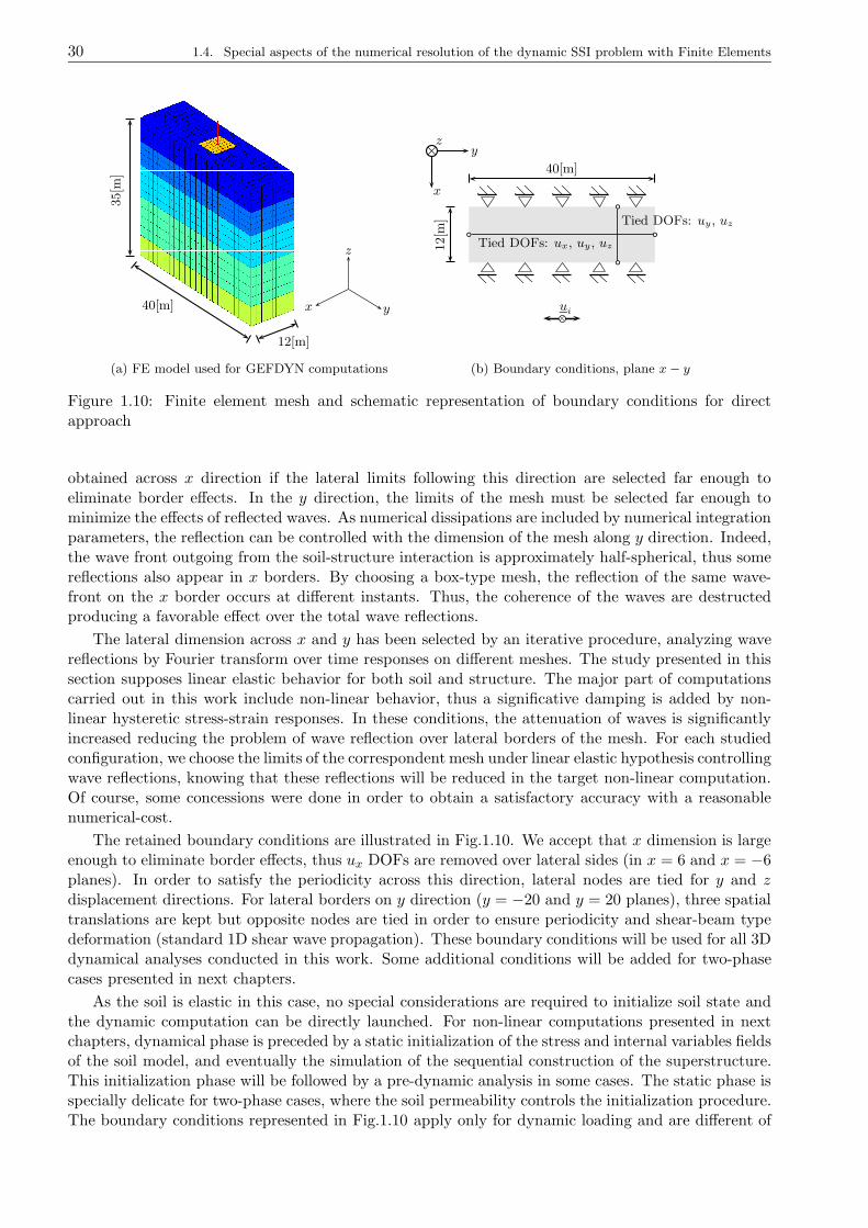
30 1.4. Special aspects of the numerical resolution of the dynamic SSI problem with Finite Elements
z
yx40[m]
12[m]
35[m
]
(a) FE model used for GEFDYN computations
y
x
×z
Tied DOFs: ux, uy , uz
Tied DOFs: uy , uz
40[m]
12[m
]
ui×
(b) Boundary conditions, plane x− y
Figure 1.10: Finite element mesh and schematic representation of boundary conditions for directapproach
obtained across x direction if the lateral limits following this direction are selected far enough toeliminate border effects. In the y direction, the limits of the mesh must be selected far enough tominimize the effects of reflected waves. As numerical dissipations are included by numerical integrationparameters, the reflection can be controlled with the dimension of the mesh along y direction. Indeed,the wave front outgoing from the soil-structure interaction is approximately half-spherical, thus somereflections also appear in x borders. By choosing a box-type mesh, the reflection of the same wave-front on the x border occurs at different instants. Thus, the coherence of the waves are destructedproducing a favorable effect over the total wave reflections.
The lateral dimension across x and y has been selected by an iterative procedure, analyzing wavereflections by Fourier transform over time responses on different meshes. The study presented in thissection supposes linear elastic behavior for both soil and structure. The major part of computationscarried out in this work include non-linear behavior, thus a significative damping is added by non-linear hysteretic stress-strain responses. In these conditions, the attenuation of waves is significantlyincreased reducing the problem of wave reflection over lateral borders of the mesh. For each studiedconfiguration, we choose the limits of the correspondent mesh under linear elastic hypothesis controllingwave reflections, knowing that these reflections will be reduced in the target non-linear computation.Of course, some concessions were done in order to obtain a satisfactory accuracy with a reasonablenumerical-cost.
The retained boundary conditions are illustrated in Fig.1.10. We accept that x dimension is largeenough to eliminate border effects, thus ux DOFs are removed over lateral sides (in x = 6 and x = −6planes). In order to satisfy the periodicity across this direction, lateral nodes are tied for y and zdisplacement directions. For lateral borders on y direction (y = −20 and y = 20 planes), three spatialtranslations are kept but opposite nodes are tied in order to ensure periodicity and shear-beam typedeformation (standard 1D shear wave propagation). These boundary conditions will be used for all 3Ddynamical analyses conducted in this work. Some additional conditions will be added for two-phasecases presented in next chapters.
As the soil is elastic in this case, no special considerations are required to initialize soil state andthe dynamic computation can be directly launched. For non-linear computations presented in nextchapters, dynamical phase is preceded by a static initialization of the stress and internal variables fieldsof the soil model, and eventually the simulation of the sequential construction of the superstructure.This initialization phase will be followed by a pre-dynamic analysis in some cases. The static phase isspecially delicate for two-phase cases, where the soil permeability controls the initialization procedure.The boundary conditions represented in Fig.1.10 apply only for dynamic loading and are different of
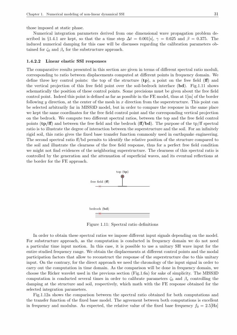
Chapter 1. Numerical modeling of non-linear dynamical SSI 31
those imposed at static phase.
Numerical integration parameters derived from one dimensional wave propagation problem de-scribed in §1.4.1 are kept, so that the a time step ∆t = 0.001[s], γ = 0.625 and β = 0.375. Theinduced numerical damping for this case will be discusses regarding the calibration parameters ob-tained for ζ0 and βs for the substructure approach.
1.4.2.2 Linear elastic SSI responses
The comparative results presented in this section are given in terms of different spectral ratio moduli,corresponding to ratio between displacements computed at different points in frequency domain. Wedefine three key control points: the top of the structure (tp), a point on the free field (ff) andthe vertical projection of this free field point over the soil-bedrock interface (bd). Fig.1.11 showsschematically the position of these control points. Some precisions must be given about the free fieldcontrol point. Indeed this point is defined as far as possible in the FE model, thus at 1[m] of the borderfollowing y direction, at the center of the mesh in x direction from the superstructure. This point canbe selected arbitrarily far in MISS3D model, but in order to compare the response in the same placewe kept the same coordinates for the free field control point and the corresponding vertical projectionon the bedrock. We compute two different spectral ratios, between the top and the free field controlpoints (tp/ff) and between the free field and the bedrock (ff/bd). The purpose of the tp/ff spectralratio is to illustrate the degree of interaction between the superstructure and the soil. For an infinitelyrigid soil, this ratio gives the fixed base transfer function commonly used in earthquake engineering.The second spectral ratio ff/bd permits to identify the relative position of the structure compared tothe soil and illustrate the clearness of the free field response, thus for a perfect free field conditionwe might not find evidences of the neighboring superstructure. The clearness of this spectral ratio iscontrolled by the generation and the attenuation of superficial waves, and its eventual reflections atthe border for the FE approach.
b×
×
×
top (tp)
free field (ff)
bedrock (bd)
Figure 1.11: Spectral ratio definitions
In order to obtain these spectral ratios we impose different input signals depending on the model.For substructure approach, as the computation is conducted in frequency domain we do not needa particular time input motion. In this case, it is possible to use a unitary SH wave input for theentire studied frequency range. We obtain the displacements at different control points and the modalparticipation factors that allow to reconstruct the response of the superstructure due to this unitaryinput. On the contrary, for the direct approach we need the chronology of the input signal in order tocarry out the computation in time domain. As the comparison will be done in frequency domain, wechoose the Ricker wavelet used in the previous section (Fig.1.6a) for sake of simplicity. The MISS3Dcomputation is conducted several times in order to calibrate parameters ζ0 and βs controlling thedamping at the structure and soil, respectively, which math with the FE response obtained for theselected integration parameters.
Fig.1.12a shows the comparison between the spectral ratio obtained for both computations andthe transfer function of the fixed base model. The agreement between both computations is excellentin frequency and modulus. As expected, the relative value of the fixed base frequency f0 = 2.5[Hz]
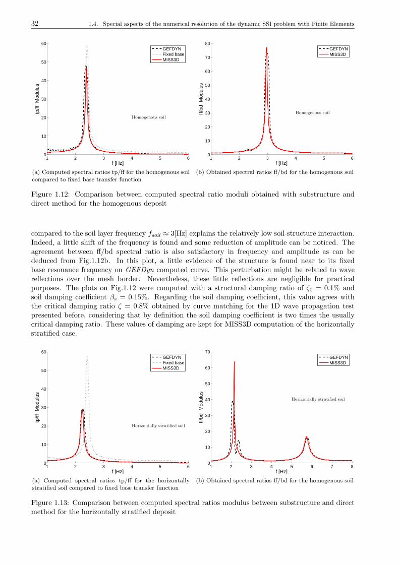
32 1.4. Special aspects of the numerical resolution of the dynamic SSI problem with Finite Elements
1 2 3 4 5 60
10
20
30
40
50
60
Homogenous soil
f [Hz]
tp/ff
Mod
ulus
GEFDYNFixed baseMISS3D
(a) Computed spectral ratios tp/ff for the homogenous soilcompared to fixed base transfer function
1 2 3 4 5 60
10
20
30
40
50
60
70
80
Homogenous soil
f [Hz]
ff/bd
Mod
ulus
GEFDYNMISS3D
(b) Obtained spectral ratios ff/bd for the homogenous soil
Figure 1.12: Comparison between computed spectral ratio moduli obtained with substructure anddirect method for the homogenous deposit
compared to the soil layer frequency fsoil ≈ 3[Hz] explains the relatively low soil-structure interaction.Indeed, a little shift of the frequency is found and some reduction of amplitude can be noticed. Theagreement between ff/bd spectral ratio is also satisfactory in frequency and amplitude as can bededuced from Fig.1.12b. In this plot, a little evidence of the structure is found near to its fixedbase resonance frequency on GEFDyn computed curve. This perturbation might be related to wavereflections over the mesh border. Nevertheless, these little reflections are negligible for practicalpurposes. The plots on Fig.1.12 were computed with a structural damping ratio of ζ0 = 0.1% andsoil damping coefficient βs = 0.15%. Regarding the soil damping coefficient, this value agrees withthe critical damping ratio ζ = 0.8% obtained by curve matching for the 1D wave propagation testpresented before, considering that by definition the soil damping coefficient is two times the usuallycritical damping ratio. These values of damping are kept for MISS3D computation of the horizontallystratified case.
1 2 3 4 5 60
10
20
30
40
50
60
Horizontally stratified soil
f [Hz]
tp/ff
Mod
ulus
GEFDYNFixed baseMISS3D
(a) Computed spectral ratios tp/ff for the horizontallystratified soil compared to fixed base transfer function
1 2 3 4 5 6 7 80
10
20
30
40
50
60
70
Horizontally stratified soil
f [Hz]
ff/bd
Mod
ulus
GEFDYNMISS3D
(b) Obtained spectral ratios ff/bd for the homogenous soil
Figure 1.13: Comparison between computed spectral ratios modulus between substructure and directmethod for the horizontally stratified deposit
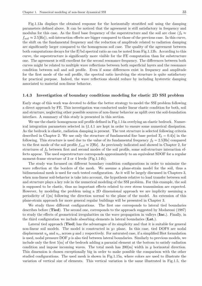
Chapter 1. Numerical modeling of non-linear dynamical SSI 33
Fig.1.13a displays the obtained response for the horizontally stratified soil using the dampingparameters defined above. It can be noticed that the agreement is still satisfactory in frequency andmodulus for this case. As the fixed base frequency of the superstructure and the soil are close (f0 ≈fsoil ≈ 2.5[Hz]), soil-interaction effects are bigger compared to those of the previous case. In this curve,the shift on the fundamental frequency and the reduction of amplitude related to radiation dampingare significantly larger compared to the homogenous soil case. The quality of the agreement betweenboth computations decays for the ff/bd spectral ratio as can be noted from Fig.1.13b. According to thiscurve, the superstructure is significantly more visible for the FE computation than for substructureone. The agreement is still excellent for the second resonance frequency. The differences between bothcurves might be related to multiple wave reflections between both superficial layers and the resonancecondition between soil and soil profile. Even if some differences exist in frequency and amplitudefor the first mode of the soil profile, the spectral ratio involving the structure is quite satisfactoryfor practical purpose. Indeed, the wave reflections should reduce by including hysteretic dampingassociated to material non-linear behavior.
1.4.3 Investigation of boundary conditions modeling for elastic 2D SSI problem
Early stage of this work was devoted to define the better strategy to model the SSI problem followinga direct approach by FE. This investigation was conducted under linear elastic condition for both, soiland structure, neglecting other possible sources of non-linear behavior as uplift over the soil-foundationinterface. A summary of this study is presented in this section.
We use the elastic homogenous soil profile defined in Fig.1.14a overlying an elastic bedrock. Numer-ical integration parameters selected in §1.4.1 are kept in order to ensure some numerical dissipation.As the bedrock is elastic, radiation damping is present. The test structure is selected following criteriadescribed in Chapter 2. We use only the structure of fundamental fixe base period T0 = 0.4[s] in thefollowing. This structure is used due to the value of its fundamental frequency f0 = 2.5[Hz] comparedto the first mode of the soil profile fsoil ≈ 2[Hz]. As previously indicated and showed in Chapter 2, forstructures of f0 between first and second modes of the soil profile, some soil-structure interaction ef-fects appear. The used superstructure corresponds approximately to an equivalent SDOF for a regularmoment-frame structure of 3 or 4 levels (Fig.1.14b).
The study was focussed on different boundary condition configurations in order to minimize thewave reflection at the borders of the mesh. We assume a plane-strain model for the soil, thus abidimensional mesh is used for each tested configuration. As it will be largely discussed in Chapters 3,when non-linear soil-behavior is take into account, the hypothesis relative to load transfer between soiland structure plays a key role in the numerical modeling of the SSI problem. For this example, the soilis supposed to be elastic, thus no important effects related to over stress transmission are expected.However, by modeling the problem using a 2D dimensional approach we are implicity assuming aperiodicity of 1[m] following the direction normal to the plane of the model. An extension of thisplane-strain approach for more general regular buildings will be presented in Chapter 3.
We study three different configurations. The first one corresponds to lateral tied boundariesdescribes before (Tied). The second one, corresponds to the approach suggested by Modaressi (1987)to study the effects of geometrical irregularities on the wave propagation in valleys (Inc.). Finally, inthe third configuration we include absorbing elements in lateral boundaries (Lat.).
Lateral tied approach (Tied) has the advantages of its simplicity and that it is suitable for generalnon-linear soil models. The model is constructed in yz plane. In this case, tied DOFS are nodaldisplacement uy and uz, across y and z respectively. For saturated case, if a simplified Biot formulationis used, nodal pressure DOF p is also tied between lateral boundaries. Similarly to previous models, weinclude only the first 5[m] of the bedrock adding a paraxial element at the bottom to satisfy radiationcondition and impose incoming waves. The total mesh has 200[m] width in y horizontal direction.This dimension is chosen exceptionally big in order to make possible the comparison with the otherstudied configurations. The used mesh is shown in Fig.1.15a, where colors are used to illustrate thevariation of vertical size of elements. This vertical variation is the same illustrated in Fig.1.5, the
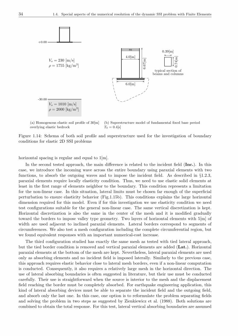
34 1.4. Special aspects of the numerical resolution of the dynamic SSI problem with Finite Elements
+0.00
-30.00
Vs = 230 [m/s]
Vs = 1010 [m/s]
ρ = 1755 [kg/m3]
ρ = 2000 [kg/m3]
(a) Homogenous elastic soil profile of 30[m]overlying elastic bedrock
6.6
7[m
]4.0[m]
6.0[m]
m0.39[m]
0.7
4[m
]
typical section ofbeams and columns
(b) Superstructure model of fundamental fixed base periodT0 = 0.4[s]
Figure 1.14: Schema of both soil profile and superstructure used for the investigation of boundaryconditions for elastic 2D SSI problems
horizontal spacing is regular and equal to 1[m].
In the second tested approach, the main difference is related to the incident field (Inc.). In thiscase, we introduce the incoming wave across the entire boundary using paraxial elements with twofunctions, to absorb the outgoing waves and to impose the incident field. As described in §1.2.3,paraxial elements require locally elasticity condition. Thus, we need to use elastic solid elements atleast in the first range of elements neighbor to the boundary. This condition represents a limitationfor the non-linear case. In this situation, lateral limits must be chosen far enough of the superficialperturbation to ensure elasticity behavior (Fig.1.15b). This conditions explains the large horizontaldimension required for this model. Even if for this investigation we use elasticity condition we needtest configurations suitable for the general non-linear case. The same vertical discretization is kept.Horizontal discretization is also the same in the center of the mesh and it is modified graduallytoward the borders to impose valley type geometry. Two layers of horizontal elements with 5[m] ofwidth are used adjacent to inclined paraxial elements. Lateral borders correspond to segments ofcircumferences. We also test a mesh configuration including the complete circumferential region, butwe found equivalent responses with an important numerical-cost increase.
The third configuration studied has exactly the same mesh as tested with tied lateral approach,but the tied border condition is removed and vertical paraxial elements are added (Lat.). Horizontalparaxial elements at the bottom of the mesh are kept. Nevertheless, lateral paraxial elements are usedonly as absorbing elements and no incident field is imposed laterally. Similarly to the previous case,this approach requires elastic behavior close to lateral mesh borders, even if a non-linear computationis conducted. Consequently, it also requires a relatively large mesh in the horizontal direction. Theuse of lateral absorbing boundaries is often suggested in literature, but their use must be conductedcarefully. Their use is straightforward when the source is interior to the mesh and the displacementfield reaching the border must be completely absorbed. For earthquake engineering application, thiskind of lateral absorbing devices must be able to separate the incident field and the outgoing field,and absorb only the last one. In this case, one option is to reformulate the problem separating fieldsand solving the problem in two steps as suggested by Zienkiewicz et al. (1988). Both solutions arecombined to obtain the total response. For this test, lateral vertical absorbing boundaries are assumed

Chapter 1. Numerical modeling of non-linear dynamical SSI 35
(a) Tied lateral boundaries approach (Tied)
(b) Valley type approach (Inc.)
(c) Lateral absorbing boundaries (Lat.)
Figure 1.15: Different 2D meshes studied in order to define the better strategy to treat lateral bound-aries in FE modeling approach
to be far enough in order to not perturb the incident field and to absorb essentially radiated wavefield. Therefore, the computation is carried out in total displacements directly.
1 2 3 4 5 60
10
20
30
40
50
60
f [Hz]
tp/ff
Mod
ulus
TiedInc.Lat.Fixed base
(a) Computed spectral ratios tp/ff for three studied config-urations
1 2 3 4 5 6 7 80
10
20
30
40
50
60
70
80
f [Hz]
ff/bd
Mod
ulus
TiedInc.Lat.
(b) Obtained spectral ratios ff/bd for three cases
Figure 1.16: Comparison between computed spectral ratio moduli for three configurations of boundaryconditions for the SSI 2D elastic case
The three computations are conducted with GEFDyn in time domain using numerical dissipativetime integration parameters. The Ricker wavelet of the Fig.1.6 is used as the incident field in allcases. The response will be compared firstly in frequency domain in terms of both spectral ratios tp/ffand ff/bd defined in previous section (Fig.1.11). Fig.1.16 shows the obtained spectral ratio modulusfor three modelled configurations compared to fixed base transfer function amplitude. As expected,significant SSI effects are visible in frequency and in amplitude. The predicted shift in the fundamentalperiod of the structure agrees for all three computations, but some differences appear concerning theamplitude. Tied approach predicts a larger reduction of amplitude, whereas Inc. and Lat. approaches
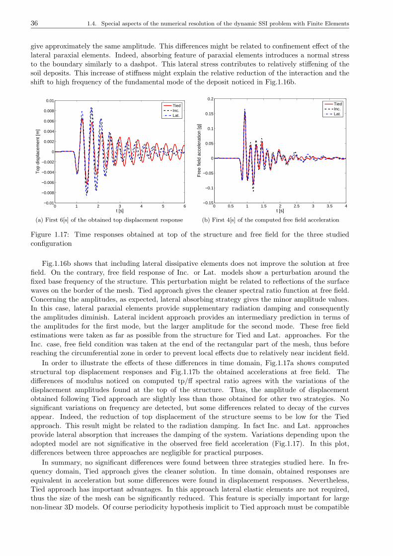
36 1.4. Special aspects of the numerical resolution of the dynamic SSI problem with Finite Elements
give approximately the same amplitude. This differences might be related to confinement effect of thelateral paraxial elements. Indeed, absorbing feature of paraxial elements introduces a normal stressto the boundary similarly to a dashpot. This lateral stress contributes to relatively stiffening of thesoil deposits. This increase of stiffness might explain the relative reduction of the interaction and theshift to high frequency of the fundamental mode of the deposit noticed in Fig.1.16b.
0 1 2 3 4 5 6−0.01
−0.008
−0.006
−0.004
−0.002
0
0.002
0.004
0.006
0.008
0.01
t [s]
Top
dis
plac
emen
t [m
]
TiedInc.Lat.
(a) First 6[s] of the obtained top displacement response
0 0.5 1 1.5 2 2.5 3 3.5 4−0.15
−0.1
−0.05
0
0.05
0.1
0.15
0.2
t [s]
Fre
e fie
ld a
ccel
erat
ion
[g]
TiedInc.Lat.
(b) First 4[s] of the computed free field acceleration
Figure 1.17: Time responses obtained at top of the structure and free field for the three studiedconfiguration
Fig.1.16b shows that including lateral dissipative elements does not improve the solution at freefield. On the contrary, free field response of Inc. or Lat. models show a perturbation around thefixed base frequency of the structure. This perturbation might be related to reflections of the surfacewaves on the border of the mesh. Tied approach gives the cleaner spectral ratio function at free field.Concerning the amplitudes, as expected, lateral absorbing strategy gives the minor amplitude values.In this case, lateral paraxial elements provide supplementary radiation damping and consequentlythe amplitudes diminish. Lateral incident approach provides an intermediary prediction in terms ofthe amplitudes for the first mode, but the larger amplitude for the second mode. These free fieldestimations were taken as far as possible from the structure for Tied and Lat. approaches. For theInc. case, free field condition was taken at the end of the rectangular part of the mesh, thus beforereaching the circumferential zone in order to prevent local effects due to relatively near incident field.
In order to illustrate the effects of these differences in time domain, Fig.1.17a shows computedstructural top displacement responses and Fig.1.17b the obtained accelerations at free field. Thedifferences of modulus noticed on computed tp/ff spectral ratio agrees with the variations of thedisplacement amplitudes found at the top of the structure. Thus, the amplitude of displacementobtained following Tied approach are slightly less than those obtained for other two strategies. Nosignificant variations on frequency are detected, but some differences related to decay of the curvesappear. Indeed, the reduction of top displacement of the structure seems to be low for the Tiedapproach. This result might be related to the radiation damping. In fact Inc. and Lat. approachesprovide lateral absorption that increases the damping of the system. Variations depending upon theadopted model are not significative in the observed free field acceleration (Fig.1.17). In this plot,differences between three approaches are negligible for practical purposes.
In summary, no significant differences were found between three strategies studied here. In fre-quency domain, Tied approach gives the cleaner solution. In time domain, obtained responses areequivalent in acceleration but some differences were found in displacement responses. Nevertheless,Tied approach has important advantages. In this approach lateral elastic elements are not required,thus the size of the mesh can be significantly reduced. This feature is specially important for largenon-linear 3D models. Of course periodicity hypothesis implicit to Tied approach must be compatible

Chapter 1. Numerical modeling of non-linear dynamical SSI 37
with the problem studied. For more complicated geometrical situations, Inc. approach will be moresuitable. The use of lateral absorbing elements is adequate when the source is interior to the mesh orif a rigid base relative-displacement approach is conducted. When the motion is imposed as incidentfield, absorbing boundaries must be treated carefully using decomposition techniques as suggested byZienkiewicz et al. (1988).
1.5 Concluding remarks
The general dynamic soil-structure interaction problem was presented theoretically by the definitionof the related governing equations in the soil and structure domains, as well as conditions over theirinterface. Special emphasis was put on dynamic boundary conditions concerning the truncation of theunbounded domain for a finite element modeling.
The constitutive models used for the numerical modeling of soil, interface and structural compo-nents were presented. These non-linear constitutive models take into account some important aspectsof the dynamic non-linear behavior of different involved materials. The used FE code GEFDyn wasenhanced by the implementation of a three dimensional plastic-hinge beam model, and the improve-ment of several other available features related to interfaces, continuous beams, sequential constructionability, among others. Special developments will be done, in order to increase the numerical capacityof the code to run costly models as presented in next chapters.
Some special aspects of the numerical modeling of the dynamical SSI problems were presented. Aswas mentioned, major issues are the treatment of the lateral boundaries and damping. These aspectswere presented in the form of 1D, 2D and 3D validations, in order to justify different modeling choicesadopted in this work.
The numerical simulations presented in this chapter were conducted in linear elasticity for both,soil and structure. Next chapters are devoted to present several non-linear applications, includingsome specific developments.

38 1.5. Concluding remarks
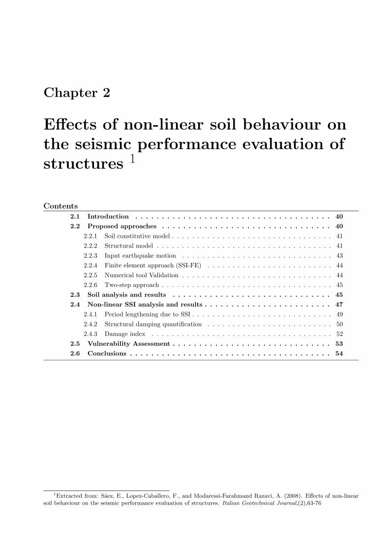
Chapter 2
Effects of non-linear soil behaviour onthe seismic performance evaluation ofstructures 1
Contents
2.1 Introduction . . . . . . . . . . . . . . . . . . . . . . . . . . . . . . . . . . . . . 40
2.2 Proposed approaches . . . . . . . . . . . . . . . . . . . . . . . . . . . . . . . . 40
2.2.1 Soil constitutive model . . . . . . . . . . . . . . . . . . . . . . . . . . . . . . . . 41
2.2.2 Structural model . . . . . . . . . . . . . . . . . . . . . . . . . . . . . . . . . . . 41
2.2.3 Input earthquake motion . . . . . . . . . . . . . . . . . . . . . . . . . . . . . . 43
2.2.4 Finite element approach (SSI-FE) . . . . . . . . . . . . . . . . . . . . . . . . . 44
2.2.5 Numerical tool Validation . . . . . . . . . . . . . . . . . . . . . . . . . . . . . . 44
2.2.6 Two-step approach . . . . . . . . . . . . . . . . . . . . . . . . . . . . . . . . . . 45
2.3 Soil analysis and results . . . . . . . . . . . . . . . . . . . . . . . . . . . . . . 45
2.4 Non-linear SSI analysis and results . . . . . . . . . . . . . . . . . . . . . . . . 47
2.4.1 Period lengthening due to SSI . . . . . . . . . . . . . . . . . . . . . . . . . . . . 49
2.4.2 Structural damping quantification . . . . . . . . . . . . . . . . . . . . . . . . . 50
2.4.3 Damage index . . . . . . . . . . . . . . . . . . . . . . . . . . . . . . . . . . . . 52
2.5 Vulnerability Assessment . . . . . . . . . . . . . . . . . . . . . . . . . . . . . . 53
2.6 Conclusions . . . . . . . . . . . . . . . . . . . . . . . . . . . . . . . . . . . . . . 54
1Extracted from: Saez, E., Lopez-Caballero, F., and Modaressi-Farahmand Razavi, A. (2008). Effects of non-linearsoil behaviour on the seismic performance evaluation of structures. Italian Geotechnical Journal,(2),63-76

40 2.1. Introduction
2.1 Introduction
In the present earthquake engineering practice, the capacity spectrum method is widely used forseismic performance evaluation of existing and new structures. Nevertheless, usually the effects ofdynamic soil-structure interaction (SSI) and the non-linear behaviour of the surrounding ground areneglected.
Some simplified procedures taking into account the dynamic SSI effects on the determination of thedesign earthquake forces and the corresponding displacements exist. For instance, FEMA 356 (2000)and ATC 40 (1996) documents give some provisions to include ground flexibility in the structuralanalysis model. Recently, FEMA 450 (2003) draft document proposes some techniques to improvethe traditional non-linear static seismic analysis. Concerning soil-structure interaction effects, thisdocument presents procedures to take into account kinematical effects as well as foundation dampingeffects. Kinematical effects are related to filtering the ground shaking transmitted to the structure i.e. amodification factor is applied to the input motion. Foundation damping is combined with the structuraldamping to obtain a revised damping for the system. All these procedures are based on traditionalsoil-structure interaction expressions with linear-elastic soil behaviour assumption. However, it iswell-known that the limit of linear-elastic soil behaviour is very low (γ < 10−5). This strain limit isnormally exceeded during a real motion.
In this work the influence of SSI effects on the seismic performance evaluation is investigated.For this purpose, numerical simulations of pushover tests and non-linear dynamic analyses (i.e. non-linearity of the soil and the structure behaviour) are performed in order to study the role of severalparameters on the seismic performance evaluation. This parametric study concerns the mechanicalproperties of the soil foundation (e.g. Vs,30 and fundamental soil deposit frequency) and the structure(i.e. fundamental period, effective height and mass) as well as the characteristics of the input motion(i.e. amplitude and frequency content). Thus, several 2D finite element computations are carried outusing non-linear elastoplastic models to represent both the soil and the structure behaviour. Resultsobtained by simplified computations performed following a two-step approach (which will be describedbelow), are compared with the ones obtained from fully non-linear time-history finite element modellinganalyses.
These results allow to identify and to quantify the differences between the two approaches. Thus, itis possible to establish the situations for which the approximate techniques might tend to overestimateor underestimate the displacement demand. We present a summary of the main findings including somerecommendations to consider in a performance evaluation following the Capacity Spectrum Method(CSM).
2.2 Proposed approaches
In order to investigate the effect of non-linear soil behaviour on seismic demand evaluation, a com-parative dynamic analysis is carried out. First, a complete finite element model including soil andstructural non-linear behaviour is used to asses the effect of non-linear dynamic soil-structure interac-tion on the structural response. Secondly, a two-step approach is carried out where: a non-linear 1Dwave propagation problem is solved for a soil column of the foundation soil. Next, the obtained freefield motion is imposed as the ground motion to a fixed base structural model. The two approachesare sketched in Fig.2.1.
The analysis is carried out for several non-linear SDOF models, with fundamental period varyingfrom 0.1[s] to 0.4[s]. The mass and height of each SDOF is obtained with typical weight and heightvalues, relating its fundamental period to the number of levels of the structure. The same infinitelyrigid shallow foundation is considered for all SDOF models.
In order to simulate the soil foundation, two non-linear homogenous dense sandy soil deposits wereused. The first one is in dry condition and the second one is fully saturated. The bedrock is placedat the depth of 30[m]. Four Europeans earthquakes are considered, scaled to different maximumoutcropping acceleration values.
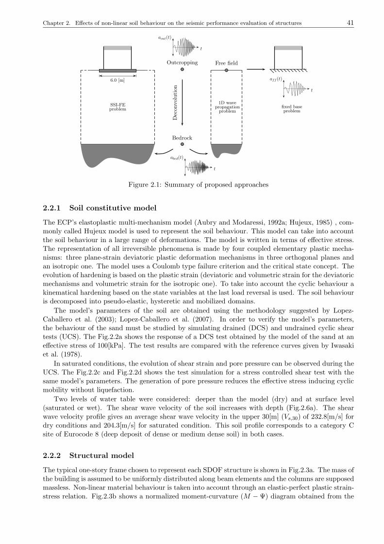
Chapter 2. Effects of non-linear soil behaviour on the seismic performance evaluation of structures 41
6.0 [m]
SSI-FEproblem
1D wavepropagation
problemfixed baseproblem
Outcropping
t
aout(t)
Dec
onvol
ution
Bedrock
t
abed(t)
Free field
t
aff (t)
Figure 2.1: Summary of proposed approaches
2.2.1 Soil constitutive model
The ECP’s elastoplastic multi-mechanism model (Aubry and Modaressi, 1992a; Hujeux, 1985) , com-monly called Hujeux model is used to represent the soil behaviour. This model can take into accountthe soil behaviour in a large range of deformations. The model is written in terms of effective stress.The representation of all irreversible phenomena is made by four coupled elementary plastic mecha-nisms: three plane-strain deviatoric plastic deformation mechanisms in three orthogonal planes andan isotropic one. The model uses a Coulomb type failure criterion and the critical state concept. Theevolution of hardening is based on the plastic strain (deviatoric and volumetric strain for the deviatoricmechanisms and volumetric strain for the isotropic one). To take into account the cyclic behaviour akinematical hardening based on the state variables at the last load reversal is used. The soil behaviouris decomposed into pseudo-elastic, hysteretic and mobilized domains.
The model’s parameters of the soil are obtained using the methodology suggested by Lopez-Caballero et al. (2003); Lopez-Caballero et al. (2007). In order to verify the model’s parameters,the behaviour of the sand must be studied by simulating drained (DCS) and undrained cyclic sheartests (UCS). The Fig.2.2a shows the response of a DCS test obtained by the model of the sand at aneffective stress of 100[kPa]. The test results are compared with the reference curves given by Iwasakiet al. (1978).
In saturated conditions, the evolution of shear strain and pore pressure can be observed during theUCS. The Fig.2.2c and Fig.2.2d shows the test simulation for a stress controlled shear test with thesame model’s parameters. The generation of pore pressure reduces the effective stress inducing cyclicmobility without liquefaction.
Two levels of water table were considered: deeper than the model (dry) and at surface level(saturated or wet). The shear wave velocity of the soil increases with depth (Fig.2.6a). The shearwave velocity profile gives an average shear wave velocity in the upper 30[m] (Vs,30) of 232.8[m/s] fordry conditions and 204.3[m/s] for saturated condition. This soil profile corresponds to a category Csite of Eurocode 8 (deep deposit of dense or medium dense soil) in both cases.
2.2.2 Structural model
The typical one-story frame chosen to represent each SDOF structure is shown in Fig.2.3a. The mass ofthe building is assumed to be uniformly distributed along beam elements and the columns are supposedmassless. Non-linear material behaviour is taken into account through an elastic-perfect plastic strain-stress relation. Fig.2.3b shows a normalized moment-curvature (M − Ψ) diagram obtained from the
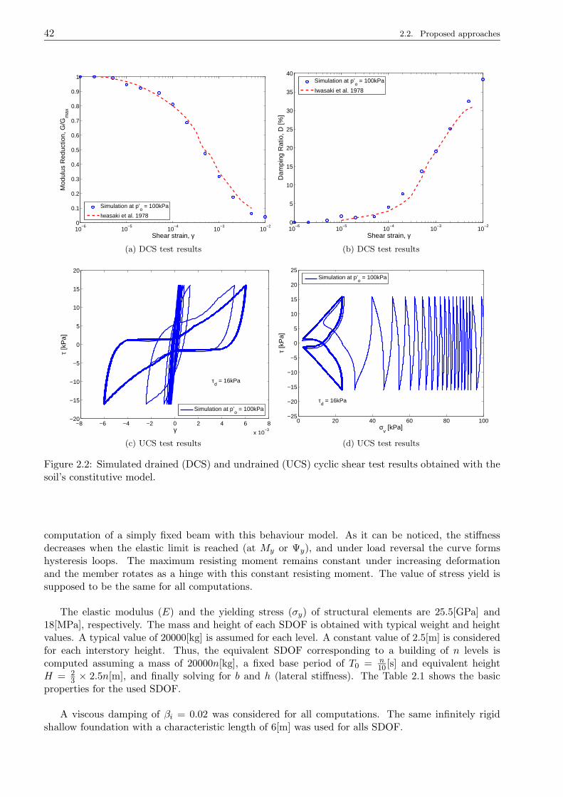
42 2.2. Proposed approaches
10−6
10−5
10−4
10−3
10−2
0
0.1
0.2
0.3
0.4
0.5
0.6
0.7
0.8
0.9
1
Shear strain, γ
Mod
ulus
Red
uctio
n, G
/Gm
ax
Simulation at p’o = 100kPa
Iwasaki et al. 1978
(a) DCS test results
10−6
10−5
10−4
10−3
10−2
0
5
10
15
20
25
30
35
40
Shear strain, γ
Dam
ping
Rat
io, D
[%]
Simulation at p’o = 100kPa
Iwasaki et al. 1978
(b) DCS test results
−8 −6 −4 −2 0 2 4 6 8
x 10−3
−20
−15
−10
−5
0
5
10
15
20
γ
τ [k
Pa]
τd = 16kPa
Simulation at p’o = 100kPa
(c) UCS test results
0 20 40 60 80 100−25
−20
−15
−10
−5
0
5
10
15
20
25
σv [kPa]
τ [k
Pa]
τd = 16kPa
Simulation at p’o = 100kPa
(d) UCS test results
Figure 2.2: Simulated drained (DCS) and undrained (UCS) cyclic shear test results obtained with thesoil’s constitutive model.
computation of a simply fixed beam with this behaviour model. As it can be noticed, the stiffnessdecreases when the elastic limit is reached (at My or Ψy), and under load reversal the curve formshysteresis loops. The maximum resisting moment remains constant under increasing deformationand the member rotates as a hinge with this constant resisting moment. The value of stress yield issupposed to be the same for all computations.
The elastic modulus (E) and the yielding stress (σy) of structural elements are 25.5[GPa] and18[MPa], respectively. The mass and height of each SDOF is obtained with typical weight and heightvalues. A typical value of 20000[kg] is assumed for each level. A constant value of 2.5[m] is consideredfor each interstory height. Thus, the equivalent SDOF corresponding to a building of n levels iscomputed assuming a mass of 20000n[kg], a fixed base period of T0 = n
10 [s] and equivalent heightH = 2
3 × 2.5n[m], and finally solving for b and h (lateral stiffness). The Table 2.1 shows the basicproperties for the used SDOF.
A viscous damping of βi = 0.02 was considered for all computations. The same infinitely rigidshallow foundation with a characteristic length of 6[m] was used for alls SDOF.
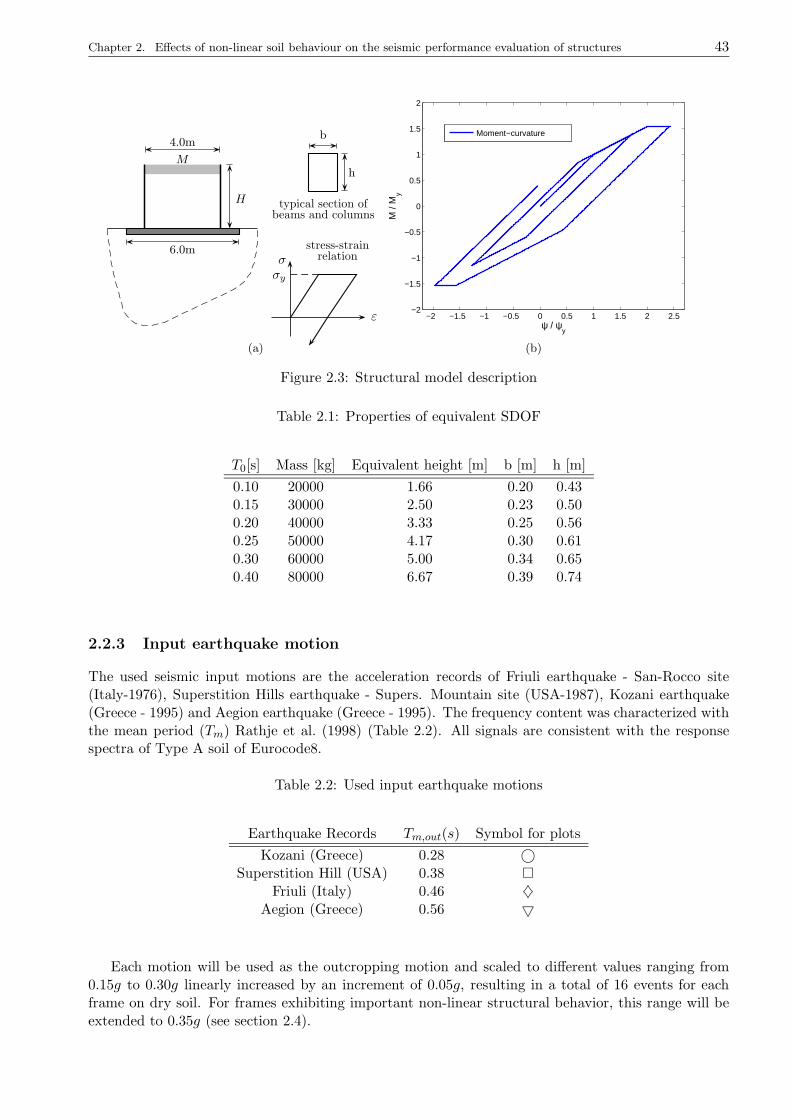
Chapter 2. Effects of non-linear soil behaviour on the seismic performance evaluation of structures 43
H
4.0m
6.0m
M
b
h
typical section ofbeams and columns
ε
σσy
stress-strainrelation
(a)
−2 −1.5 −1 −0.5 0 0.5 1 1.5 2 2.5−2
−1.5
−1
−0.5
0
0.5
1
1.5
2
ψ / ψy
M /
My
Moment−curvature
(b)
Figure 2.3: Structural model description
Table 2.1: Properties of equivalent SDOF
T0[s] Mass [kg] Equivalent height [m] b [m] h [m]
0.10 20000 1.66 0.20 0.430.15 30000 2.50 0.23 0.500.20 40000 3.33 0.25 0.560.25 50000 4.17 0.30 0.610.30 60000 5.00 0.34 0.650.40 80000 6.67 0.39 0.74
2.2.3 Input earthquake motion
The used seismic input motions are the acceleration records of Friuli earthquake - San-Rocco site(Italy-1976), Superstition Hills earthquake - Supers. Mountain site (USA-1987), Kozani earthquake(Greece - 1995) and Aegion earthquake (Greece - 1995). The frequency content was characterized withthe mean period (Tm) Rathje et al. (1998) (Table 2.2). All signals are consistent with the responsespectra of Type A soil of Eurocode8.
Table 2.2: Used input earthquake motions
Earthquake Records Tm,out(s) Symbol for plots
Kozani (Greece) 0.28 ©Superstition Hill (USA) 0.38
Friuli (Italy) 0.46 ♦Aegion (Greece) 0.56
Each motion will be used as the outcropping motion and scaled to different values ranging from0.15g to 0.30g linearly increased by an increment of 0.05g, resulting in a total of 16 events for eachframe on dry soil. For frames exhibiting important non-linear structural behavior, this range will beextended to 0.35g (see section 2.4).
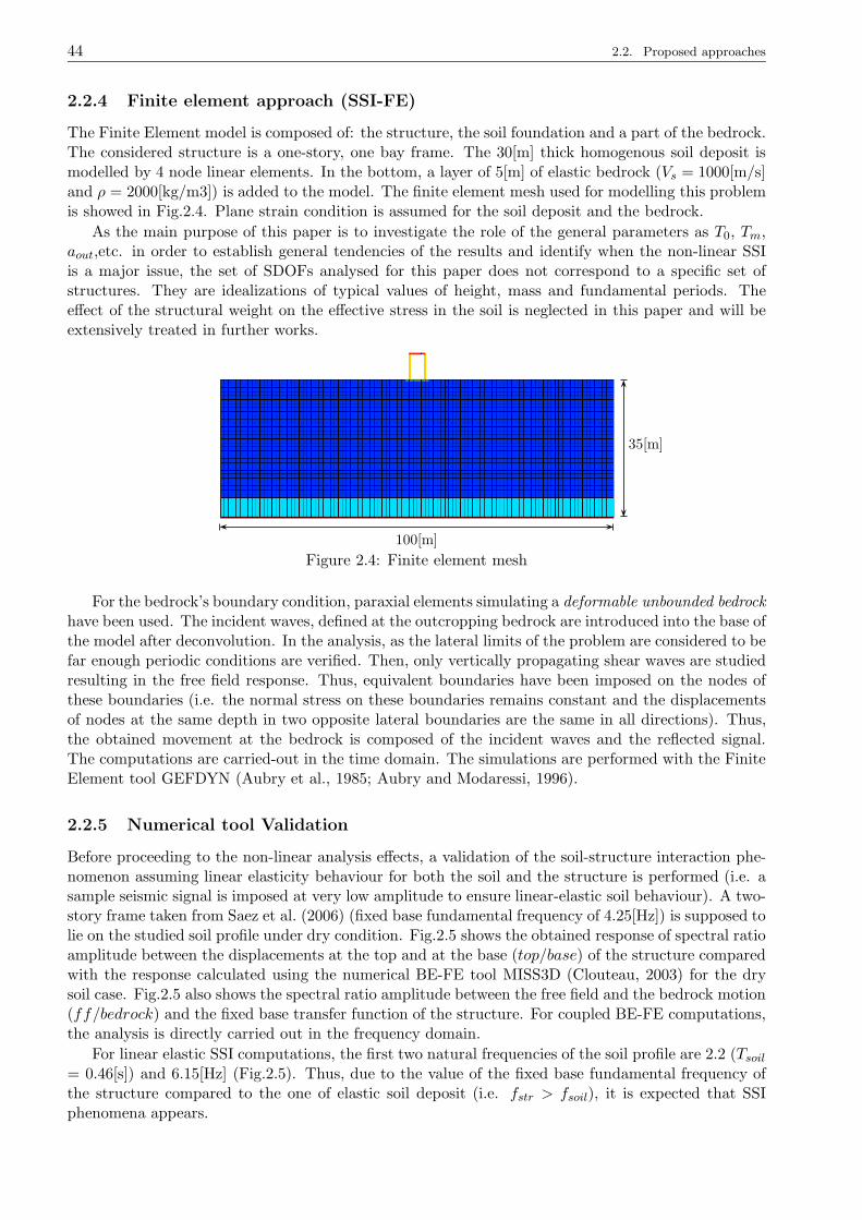
44 2.2. Proposed approaches
2.2.4 Finite element approach (SSI-FE)
The Finite Element model is composed of: the structure, the soil foundation and a part of the bedrock.The considered structure is a one-story, one bay frame. The 30[m] thick homogenous soil deposit ismodelled by 4 node linear elements. In the bottom, a layer of 5[m] of elastic bedrock (Vs = 1000[m/s]and ρ = 2000[kg/m3]) is added to the model. The finite element mesh used for modelling this problemis showed in Fig.2.4. Plane strain condition is assumed for the soil deposit and the bedrock.
As the main purpose of this paper is to investigate the role of the general parameters as T0, Tm,aout,etc. in order to establish general tendencies of the results and identify when the non-linear SSIis a major issue, the set of SDOFs analysed for this paper does not correspond to a specific set ofstructures. They are idealizations of typical values of height, mass and fundamental periods. Theeffect of the structural weight on the effective stress in the soil is neglected in this paper and will beextensively treated in further works.
100[m]
35[m]
Figure 2.4: Finite element mesh
For the bedrock’s boundary condition, paraxial elements simulating a deformable unbounded bedrockhave been used. The incident waves, defined at the outcropping bedrock are introduced into the base ofthe model after deconvolution. In the analysis, as the lateral limits of the problem are considered to befar enough periodic conditions are verified. Then, only vertically propagating shear waves are studiedresulting in the free field response. Thus, equivalent boundaries have been imposed on the nodes ofthese boundaries (i.e. the normal stress on these boundaries remains constant and the displacementsof nodes at the same depth in two opposite lateral boundaries are the same in all directions). Thus,the obtained movement at the bedrock is composed of the incident waves and the reflected signal.The computations are carried-out in the time domain. The simulations are performed with the FiniteElement tool GEFDYN (Aubry et al., 1985; Aubry and Modaressi, 1996).
2.2.5 Numerical tool Validation
Before proceeding to the non-linear analysis effects, a validation of the soil-structure interaction phe-nomenon assuming linear elasticity behaviour for both the soil and the structure is performed (i.e. asample seismic signal is imposed at very low amplitude to ensure linear-elastic soil behaviour). A two-story frame taken from Saez et al. (2006) (fixed base fundamental frequency of 4.25[Hz]) is supposed tolie on the studied soil profile under dry condition. Fig.2.5 shows the obtained response of spectral ratioamplitude between the displacements at the top and at the base (top/base) of the structure comparedwith the response calculated using the numerical BE-FE tool MISS3D (Clouteau, 2003) for the drysoil case. Fig.2.5 also shows the spectral ratio amplitude between the free field and the bedrock motion(ff/bedrock) and the fixed base transfer function of the structure. For coupled BE-FE computations,the analysis is directly carried out in the frequency domain.
For linear elastic SSI computations, the first two natural frequencies of the soil profile are 2.2 (Tsoil= 0.46[s]) and 6.15[Hz] (Fig.2.5). Thus, due to the value of the fixed base fundamental frequency ofthe structure compared to the one of elastic soil deposit (i.e. fstr > fsoil), it is expected that SSIphenomena appears.
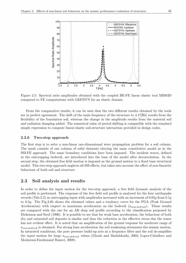
Chapter 2. Effects of non-linear soil behaviour on the seismic performance evaluation of structures 45
1.5 2 2.5 3 3.5 4 4.5 5 5.5 6 6.50
10
20
30
40
50
60
70
80
90
100
f [Hz]
Spe
ctra
l Rat
io A
mpl
itude
GEFDYN: ff/bedrockMISS3D: top/baseGEFDYN: top/baseGEFDYN: fixed base
Figure 2.5: Spectral ratio amplitudes obtained with the coupled BE-FE linear elastic tool MISS3Dcompared to FE computations with GEFDYN for an elastic domain.
From the comparative results, it can be seen that the two different results obtained by the toolsare in perfect agreement. The shift of the main frequency of the structure to 4.17[Hz] results from theflexibility of the foundation soil, whereas the change in the amplitude results from the material soiland radiation damping added. The numerical value of period shifting is compatible with the standardsimple expression to compute linear-elastic soil-structure interaction provided in design codes.
2.2.6 Two-step approach
The first step is to solve a non-linear one-dimensional wave propagation problem for a soil column.The mesh consists of one column of solid elements obeying the same constitutive model as in theSSI-FE approach. The same boundary conditions have been imposed. The incident waves, definedat the outcropping bedrock, are introduced into the base of the model after deconvolution. In thesecond step, the obtained free field motion is imposed as the ground motion to a fixed base structuralmodel. This two-step approach neglects all SSI effects, but takes into account the effect of non-linearitybehaviour of both soil and structure.
2.3 Soil analysis and results
In order to define the input motion for the two-step approach, a free field dynamic analysis of thesoil profile is performed. The response of the free field soil profile is analysed for the four earthquakerecords (Tab.2.2) as outcropping input with amplitudes increased with an increment of 0.05g from 0.1gto 0.5g. The Fig.2.6b shows the obtained values and a tendency curve for the PGA (Peak GroundAcceleration) with respect to maximum acceleration on the bedrock (amax,bedrock). These resultsare compared with the one for an AB deep soil profile according to the classification proposed byDickenson and Seed (1996). It is possible to see that for weak base acceleration, the behaviour of bothdry and saturated soil deposits is similar and thus the reduction in the effective stress due the waterhas not evident effect. It is noted that an amplification of the ground response for moderate range ofamax,bedrock is obtained. For strong base acceleration the soil weakening attenuates the seismic motion.In saturated conditions, the pore pressure build-up acts as a frequency filter and the soil de-amplifiesthe input motion for large amax,bedrock values (Ghosh and Madabhushi, 2003; Lopez-Caballero andModaressi-Farahmand Razavi, 2008).
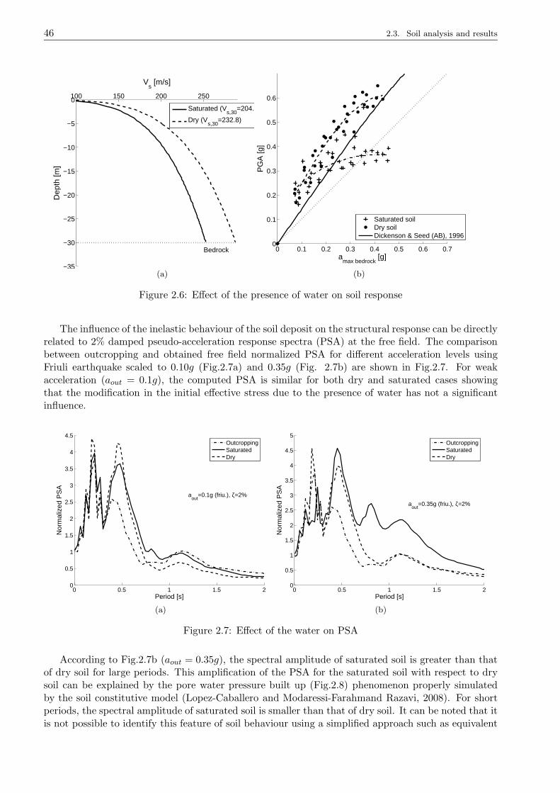
46 2.3. Soil analysis and results
100 150 200 250
−35
−30
−25
−20
−15
−10
−5
0
Bedrock
Vs [m/s]
Dep
th [m
]
Saturated (Vs,30
=204.3)
Dry (Vs,30
=232.8)
(a)
0 0.1 0.2 0.3 0.4 0.5 0.6 0.70
0.1
0.2
0.3
0.4
0.5
0.6
amax bedrock
[g]P
GA
[g]
Saturated soilDry soilDickenson & Seed (AB), 1996
(b)
Figure 2.6: Effect of the presence of water on soil response
The influence of the inelastic behaviour of the soil deposit on the structural response can be directlyrelated to 2% damped pseudo-acceleration response spectra (PSA) at the free field. The comparisonbetween outcropping and obtained free field normalized PSA for different acceleration levels usingFriuli earthquake scaled to 0.10g (Fig.2.7a) and 0.35g (Fig. 2.7b) are shown in Fig.2.7. For weakacceleration (aout = 0.1g), the computed PSA is similar for both dry and saturated cases showingthat the modification in the initial effective stress due to the presence of water has not a significantinfluence.
0 0.5 1 1.5 20
0.5
1
1.5
2
2.5
3
3.5
4
4.5
aout
=0.1g (friu.), ζ=2%
Nor
mal
ized
PS
A
Period [s]
OutcroppingSaturatedDry
(a)
0 0.5 1 1.5 20
0.5
1
1.5
2
2.5
3
3.5
4
4.5
5
aout
=0.35g (friu.), ζ=2%
Nor
mal
ized
PS
A
Period [s]
OutcroppingSaturatedDry
(b)
Figure 2.7: Effect of the water on PSA
According to Fig.2.7b (aout = 0.35g), the spectral amplitude of saturated soil is greater than thatof dry soil for large periods. This amplification of the PSA for the saturated soil with respect to drysoil can be explained by the pore water pressure built up (Fig.2.8) phenomenon properly simulatedby the soil constitutive model (Lopez-Caballero and Modaressi-Farahmand Razavi, 2008). For shortperiods, the spectral amplitude of saturated soil is smaller than that of dry soil. It can be noted that itis not possible to identify this feature of soil behaviour using a simplified approach such as equivalent
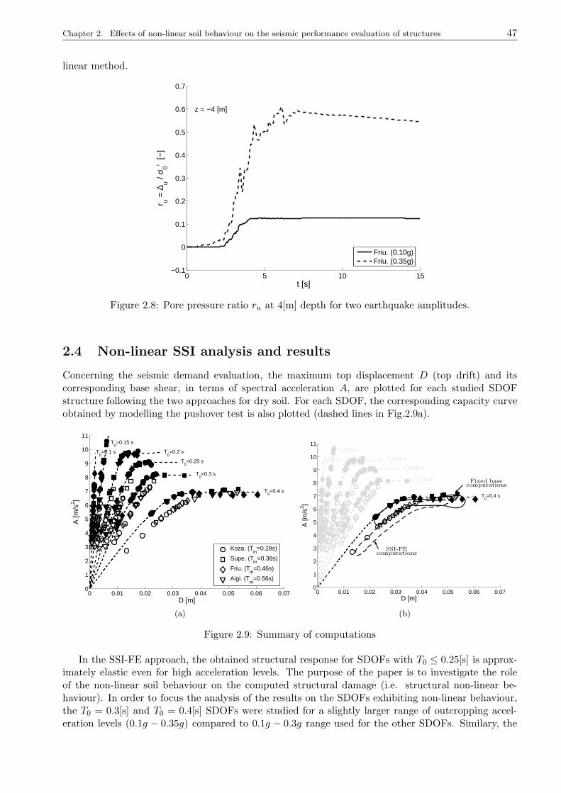
Chapter 2. Effects of non-linear soil behaviour on the seismic performance evaluation of structures 47
linear method.
0 5 10 15−0.1
0
0.1
0.2
0.3
0.4
0.5
0.6
0.7
z = −4 [m]
t [s]
r u = ∆
u / σ 0’
[−]
Friu. (0.10g)Friu. (0.35g)
Figure 2.8: Pore pressure ratio ru at 4[m] depth for two earthquake amplitudes.
2.4 Non-linear SSI analysis and results
Concerning the seismic demand evaluation, the maximum top displacement D (top drift) and itscorresponding base shear, in terms of spectral acceleration A, are plotted for each studied SDOFstructure following the two approaches for dry soil. For each SDOF, the corresponding capacity curveobtained by modelling the pushover test is also plotted (dashed lines in Fig.2.9a).
0 0.01 0.02 0.03 0.04 0.05 0.06 0.070
1
2
3
4
5
6
7
8
9
10
11
T0=0.1 s
T0=0.15 s
T0=0.2 s
T0=0.25 s
T0=0.3 s
T0=0.4 s
D [m]
A [m
/s2 ]
Koza. (Tm
=0.28s)
Supe. (Tm
=0.38s)
Friu. (Tm
=0.46s)
Aigi. (Tm
=0.56s)
(a)
0 0.01 0.02 0.03 0.04 0.05 0.06 0.070
1
2
3
4
5
6
7
8
9
10
11
T0=0.1 s
T0=0.15 s
T0=0.2 s
T0=0.25 s
T0=0.3 s
T0=0.4 s
D [m]
A [m
/s2 ]
Fixed basecomputations
SSI-FEcomputations
(b)
Figure 2.9: Summary of computations
In the SSI-FE approach, the obtained structural response for SDOFs with T0 ≤ 0.25[s] is approx-imately elastic even for high acceleration levels. The purpose of the paper is to investigate the roleof the non-linear soil behaviour on the computed structural damage (i.e. structural non-linear be-haviour). In order to focus the analysis of the results on the SDOFs exhibiting non-linear behaviour,the T0 = 0.3[s] and T0 = 0.4[s] SDOFs were studied for a slightly larger range of outcropping accel-eration levels (0.1g − 0.35g) compared to 0.1g − 0.3g range used for the other SDOFs. Similary, the
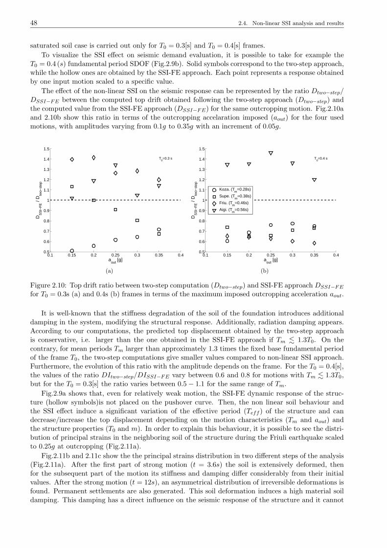
48 2.4. Non-linear SSI analysis and results
saturated soil case is carried out only for T0 = 0.3[s] and T0 = 0.4[s] frames.
To visualize the SSI effect on seismic demand evaluation, it is possible to take for example theT0 = 0.4 (s) fundamental period SDOF (Fig.2.9b). Solid symbols correspond to the two-step approach,while the hollow ones are obtained by the SSI-FE approach. Each point represents a response obtainedby one input motion scaled to a specific value.
The effect of the non-linear SSI on the seismic response can be represented by the ratio Dtwo−step/DSSI−FE between the computed top drift obtained following the two-step approach (Dtwo−step) andthe computed value from the SSI-FE approach (DSSI−FE) for the same outcropping motion. Fig.2.10aand 2.10b show this ratio in terms of the outcropping accelaration imposed (aout) for the four usedmotions, with amplitudes varying from 0.1g to 0.35g with an increment of 0.05g.
0.1 0.15 0.2 0.25 0.3 0.35 0.40.5
0.6
0.7
0.8
0.9
1
1.1
1.2
1.3
1.4
1.5
T0=0.3 s
aout
[g]
DS
SI−
FE /
Dtw
o−st
ep
(a)
0.1 0.15 0.2 0.25 0.3 0.35 0.40.5
0.6
0.7
0.8
0.9
1
1.1
1.2
1.3
1.4
1.5
T0=0.4 s
aout
[g]
DS
SI−
FE /
Dtw
o−st
ep
Koza. (Tm
=0.28s)
Supe. (Tm
=0.38s)
Friu. (Tm
=0.46s)
Aigi. (Tm
=0.56s)
(b)
Figure 2.10: Top drift ratio between two-step computation (Dtwo−step) and SSI-FE approach DSSI−FEfor T0 = 0.3s (a) and 0.4s (b) frames in terms of the maximum imposed outcropping acceleration aout.
It is well-known that the stiffness degradation of the soil of the foundation introduces additionaldamping in the system, modifying the structural response. Additionally, radiation damping appears.According to our computations, the predicted top displacement obtained by the two-step approachis conservative, i.e. larger than the one obtained in the SSI-FE approach if Tm . 1.3T0. On thecontrary, for mean periods Tm larger than approximately 1.3 times the fixed base fundamental periodof the frame T0, the two-step computations give smaller values compared to non-linear SSI approach.Furthermore, the evolution of this ratio with the amplitude depends on the frame. For the T0 = 0.4[s],the values of the ratio DItwo−step/DISSI−FE vary between 0.6 and 0.8 for motions with Tm . 1.3T0,but for the T0 = 0.3[s] the ratio varies between 0.5 − 1.1 for the same range of Tm.
Fig.2.9a shows that, even for relatively weak motion, the SSI-FE dynamic response of the struc-ture (hollow symbols)is not placed on the pushover curve. Then, the non linear soil behaviour andthe SSI effect induce a significant variation of the effective period (Teff ) of the structure and candecrease/increase the top displacement depending on the motion characteristics (Tm and aout) andthe structure properties (T0 and m). In order to explain this behaviour, it is possible to see the distri-bution of principal strains in the neighboring soil of the structure during the Friuli earthquake scaledto 0.25g at outcropping (Fig.2.11a).
Fig.2.11b and 2.11c show the the principal strains distribution in two different steps of the analysis(Fig.2.11a). After the first part of strong motion (t = 3.6s) the soil is extensively deformed, thenfor the subsequent part of the motion its stiffness and damping differ considerably from their initialvalues. After the strong motion (t = 12s), an asymmetrical distribution of irreversible deformations isfound. Permanent settlements are also generated. This soil deformation induces a high material soildamping. This damping has a direct influence on the seismic response of the structure and it cannot
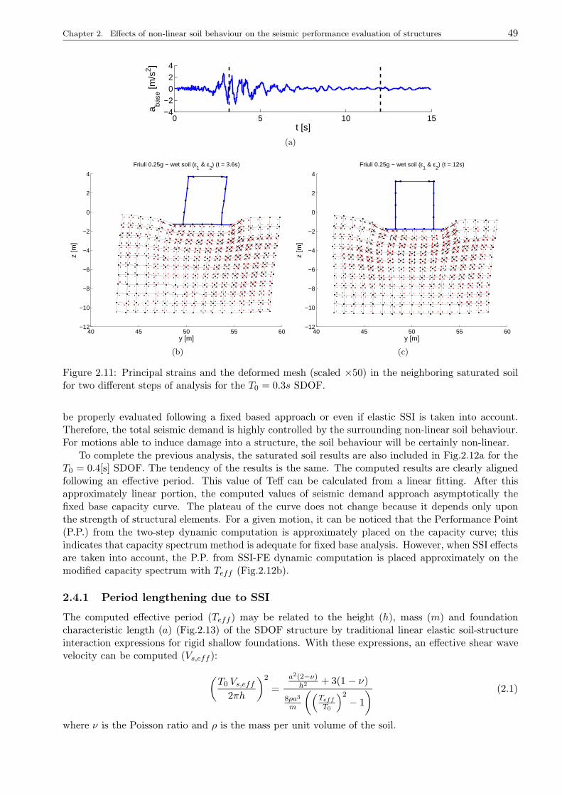
Chapter 2. Effects of non-linear soil behaviour on the seismic performance evaluation of structures 49
0 5 10 15−4−2
024
a base
[m/s
2 ]
t [s]
(a)
40 45 50 55 60−12
−10
−8
−6
−4
−2
0
2
4
y [m]
z [m
]
Friuli 0.25g − wet soil (ε1 & ε
2) (t = 3.6s)
(b)
40 45 50 55 60−12
−10
−8
−6
−4
−2
0
2
4
y [m]
z [m
]
Friuli 0.25g − wet soil (ε1 & ε
2) (t = 12s)
(c)
Figure 2.11: Principal strains and the deformed mesh (scaled ×50) in the neighboring saturated soilfor two different steps of analysis for the T0 = 0.3s SDOF.
be properly evaluated following a fixed based approach or even if elastic SSI is taken into account.Therefore, the total seismic demand is highly controlled by the surrounding non-linear soil behaviour.For motions able to induce damage into a structure, the soil behaviour will be certainly non-linear.
To complete the previous analysis, the saturated soil results are also included in Fig.2.12a for theT0 = 0.4[s] SDOF. The tendency of the results is the same. The computed results are clearly alignedfollowing an effective period. This value of Teff can be calculated from a linear fitting. After thisapproximately linear portion, the computed values of seismic demand approach asymptotically thefixed base capacity curve. The plateau of the curve does not change because it depends only uponthe strength of structural elements. For a given motion, it can be noticed that the Performance Point(P.P.) from the two-step dynamic computation is approximately placed on the capacity curve; thisindicates that capacity spectrum method is adequate for fixed base analysis. However, when SSI effectsare taken into account, the P.P. from SSI-FE dynamic computation is placed approximately on themodified capacity spectrum with Teff (Fig.2.12b).
2.4.1 Period lengthening due to SSI
The computed effective period (Teff ) may be related to the height (h), mass (m) and foundationcharacteristic length (a) (Fig.2.13) of the SDOF structure by traditional linear elastic soil-structureinteraction expressions for rigid shallow foundations. With these expressions, an effective shear wavevelocity can be computed (Vs,eff ):
(T0 Vs,eff
2πh
)2
=
a2(2−ν)h2 + 3(1 − ν)
8ρa3
m
((Teff
T0
)2− 1
) (2.1)
where ν is the Poisson ratio and ρ is the mass per unit volume of the soil.

50 2.4. Non-linear SSI analysis and results
0 0.01 0.02 0.03 0.04 0.05 0.06 0.070
1
2
3
4
5
6
7
8
9
T0=0.4 s → T
eff=0.448 s → V
s,eff=149.2 m/s
D [m]
A [m
/s2 ]
Dry (SSI−FE)Sat. (SSI−FE)Dry (fixed base)Sat. (fixed base)
Fixed base
SSI-FE
Capacity curve
(a)
D
A
PSA(
βeq,fb
)
PSA(
βeq,ssi
)
b
T0
Teff
Fixed baseP.P.
b
SSI-FEP.P.
(b)
Figure 2.12: Summary of results
m
h
a
Vs,eff , ρ, ν = cte.
Figure 2.13: Geometrical scheme
It is possible to obtain for each SDOF, the variation of effective period and effective shear wavevelocity.
According to Fig.2.14a, soil-structure interaction effects seem important only for structures withelastic periods placed between the two first elastic periods of the soil deposit (T 1
soil and T 2soil). For
periods smaller than the second period of soil, the effective periods approach quickly that of the fixedbase value. The ratio between the fixed base value and effective value is near to 90% for this type ofsoil.
From Fig.2.14b, it can be noticed that the effective shear wave velocity is approximately constantfor structures with fundamental periods between the two first ones of the soil. This value can beconsidered like approximately constant and equal to two third of Vs,30 Eurocode 8’s parameter in thiscase. Then, according to our results, a typical value of 2
3Vs,30 into traditional elastic SSI relations canbe used to compute an effective period for the used SDOFs.
2.4.2 Structural damping quantification
The application of the CSM procedure implies the computation of an equivalent viscous dampingcoefficient at the performance point (βeq). This parameter includes the inherent structural damping(βi) and the damping related to the damage of the structure (β0).
A bilinear representation of the capacity spectrum is constructed following ATC-40 guidelines toestimate β0 (Fig.2.15a). The values of β0 are computed using fixed base capacity spectrum. Fig.2.15bshow the computed values of damping as a function of the peak ground acceleration at the free field(amax,ff ) (solid symbols on Fig.2.15b). For SSI-FE computations, the capacity spectrum curve fittedusing the obtained results of the dynamic SSI computations was used. With this capacity spectrum,the equivalent viscous damping β0 values are also computed using the bilinear approximation suggestedby ATC-40 (hollow symbols on Fig.2.15b). Some cases exhibiting structural linear behaviour have been
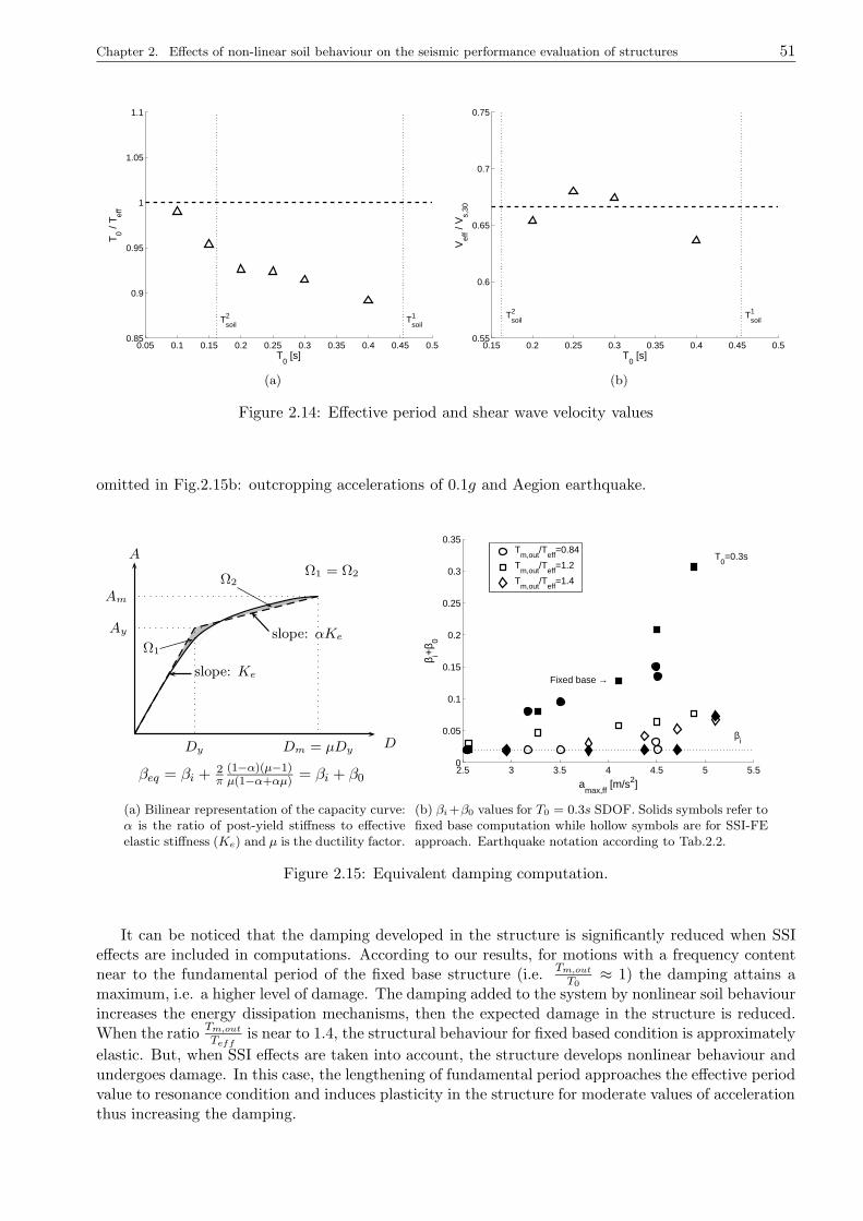
Chapter 2. Effects of non-linear soil behaviour on the seismic performance evaluation of structures 51
0.05 0.1 0.15 0.2 0.25 0.3 0.35 0.4 0.45 0.50.85
0.9
0.95
1
1.05
1.1
Tsoil1T
soil2
T0 [s]
T0 /
T eff
(a)
0.15 0.2 0.25 0.3 0.35 0.4 0.45 0.50.55
0.6
0.65
0.7
0.75
Tsoil1T
soil2
T0 [s]
Vef
f / V
s,30
(b)
Figure 2.14: Effective period and shear wave velocity values
omitted in Fig.2.15b: outcropping accelerations of 0.1g and Aegion earthquake.
D
A
Am
Dm = µDy
Ay
slope: Ke
slope: αKe
Dy
Ω1
Ω2Ω1 = Ω2
βeq = βi +2π
(1−α)(µ−1)µ(1−α+αµ) = βi + β0
(a) Bilinear representation of the capacity curve:α is the ratio of post-yield stiffness to effectiveelastic stiffness (Ke) and µ is the ductility factor.
2.5 3 3.5 4 4.5 5 5.50
0.05
0.1
0.15
0.2
0.25
0.3
0.35
βi
T0=0.3s
Fixed base →
amax,ff
[m/s2]
β i+β 0
Tm,out
/Teff
=0.84
Tm,out
/Teff
=1.2
Tm,out
/Teff
=1.4
(b) βi +β0 values for T0 = 0.3s SDOF. Solids symbols refer tofixed base computation while hollow symbols are for SSI-FEapproach. Earthquake notation according to Tab.2.2.
Figure 2.15: Equivalent damping computation.
It can be noticed that the damping developed in the structure is significantly reduced when SSIeffects are included in computations. According to our results, for motions with a frequency contentnear to the fundamental period of the fixed base structure (i.e.
Tm,out
T0≈ 1) the damping attains a
maximum, i.e. a higher level of damage. The damping added to the system by nonlinear soil behaviourincreases the energy dissipation mechanisms, then the expected damage in the structure is reduced.When the ratio
Tm,out
Teffis near to 1.4, the structural behaviour for fixed based condition is approximately
elastic. But, when SSI effects are taken into account, the structure develops nonlinear behaviour andundergoes damage. In this case, the lengthening of fundamental period approaches the effective periodvalue to resonance condition and induces plasticity in the structure for moderate values of accelerationthus increasing the damping.
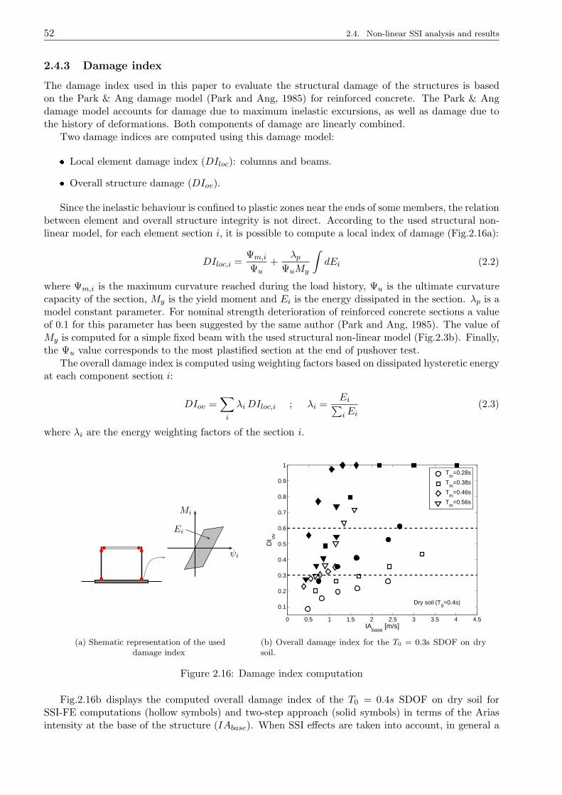
52 2.4. Non-linear SSI analysis and results
2.4.3 Damage index
The damage index used in this paper to evaluate the structural damage of the structures is basedon the Park & Ang damage model (Park and Ang, 1985) for reinforced concrete. The Park & Angdamage model accounts for damage due to maximum inelastic excursions, as well as damage due tothe history of deformations. Both components of damage are linearly combined.
Two damage indices are computed using this damage model: Local element damage index (DIloc): columns and beams. Overall structure damage (DIov).
Since the inelastic behaviour is confined to plastic zones near the ends of some members, the relationbetween element and overall structure integrity is not direct. According to the used structural non-linear model, for each element section i, it is possible to compute a local index of damage (Fig.2.16a):
DIloc,i =Ψm,i
Ψu+
λpΨuMy
∫
dEi (2.2)
where Ψm,i is the maximum curvature reached during the load history, Ψu is the ultimate curvaturecapacity of the section, My is the yield moment and Ei is the energy dissipated in the section. λp is amodel constant parameter. For nominal strength deterioration of reinforced concrete sections a valueof 0.1 for this parameter has been suggested by the same author (Park and Ang, 1985). The value ofMy is computed for a simple fixed beam with the used structural non-linear model (Fig.2.3b). Finally,the Ψu value corresponds to the most plastified section at the end of pushover test.
The overall damage index is computed using weighting factors based on dissipated hysteretic energyat each component section i:
DIov =∑
i
λiDIloc,i ; λi =Ei∑
iEi(2.3)
where λi are the energy weighting factors of the section i.
b b
b bb b
Mi
ψi
Ei
(a) Shematic representation of the useddamage index
0 0.5 1 1.5 2 2.5 3 3.5 4 4.5
0.1
0.2
0.3
0.4
0.5
0.6
0.7
0.8
0.9
1
IAbase
[m/s]
DI ov
Dry soil (T0=0.4s)
Tm
=0.28s
Tm
=0.38s
Tm
=0.46s
Tm
=0.56s
(b) Overall damage index for the T0 = 0.3s SDOF on drysoil.
Figure 2.16: Damage index computation
Fig.2.16b displays the computed overall damage index of the T0 = 0.4s SDOF on dry soil forSSI-FE computations (hollow symbols) and two-step approach (solid symbols) in terms of the Ariasintensity at the base of the structure (IAbase). When SSI effects are taken into account, in general a
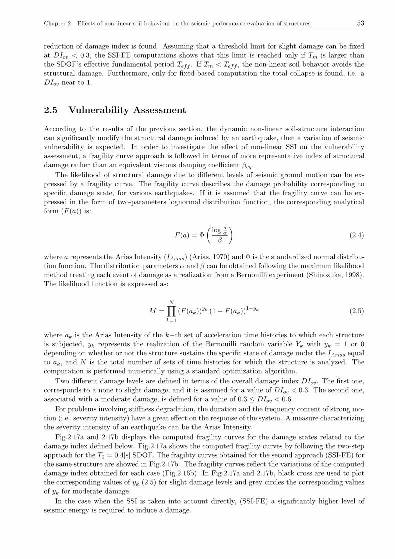
Chapter 2. Effects of non-linear soil behaviour on the seismic performance evaluation of structures 53
reduction of damage index is found. Assuming that a threshold limit for slight damage can be fixedat DIov < 0.3, the SSI-FE computations shows that this limit is reached only if Tm is larger thanthe SDOF’s effective fundamental period Teff . If Tm < Teff , the non-linear soil behavior avoids thestructural damage. Furthermore, only for fixed-based computation the total collapse is found, i.e. aDIov near to 1.
2.5 Vulnerability Assessment
According to the results of the previous section, the dynamic non-linear soil-structure interactioncan significantly modify the structural damage induced by an earthquake, then a variation of seismicvulnerability is expected. In order to investigate the effect of non-linear SSI on the vulnerabilityassessment, a fragility curve approach is followed in terms of more representative index of structuraldamage rather than an equivalent viscous damping coefficient βeq.
The likelihood of structural damage due to different levels of seismic ground motion can be ex-pressed by a fragility curve. The fragility curve describes the damage probability corresponding tospecific damage state, for various earthquakes. If it is assumed that the fragility curve can be ex-pressed in the form of two-parameters lognormal distribution function, the corresponding analyticalform (F (a)) is:
F (a) = Φ
(log a
α
β
)
(2.4)
where a represents the Arias Intensity (IArias) (Arias, 1970) and Φ is the standardized normal distribu-tion function. The distribution parameters α and β can be obtained following the maximum likelihoodmethod treating each event of damage as a realization from a Bernouilli experiment (Shinozuka, 1998).The likelihood function is expressed as:
M =N∏
k=1
(F (ak))yk (1− F (ak))
1−yk (2.5)
where ak is the Arias Intensity of the k−th set of acceleration time histories to which each structureis subjected, yk represents the realization of the Bernouilli random variable Yk with yk = 1 or 0depending on whether or not the structure sustains the specific state of damage under the IArias equalto ak, and N is the total number of sets of time histories for which the structure is analyzed. Thecomputation is performed numerically using a standard optimization algorithm.
Two different damage levels are defined in terms of the overall damage index DIov. The first one,corresponds to a none to slight damage, and it is assumed for a value of DIov < 0.3. The second one,associated with a moderate damage, is defined for a value of 0.3 ≤ DIov < 0.6.
For problems involving stiffness degradation, the duration and the frequency content of strong mo-tion (i.e. severity intensity) have a great effect on the response of the system. A measure characterizingthe severity intensity of an earthquake can be the Arias Intensity.
Fig.2.17a and 2.17b displays the computed fragility curves for the damage states related to thedamage index defined below. Fig.2.17a shows the computed fragility curves by following the two-stepapproach for the T0 = 0.4[s] SDOF. The fragility curves obtained for the second approach (SSI-FE) forthe same structure are showed in Fig.2.17b. The fragility curves reflect the variations of the computeddamage index obtained for each case (Fig.2.16b). In Fig.2.17a and 2.17b, black cross are used to plotthe corresponding values of yk (2.5) for slight damage levels and grey circles the corresponding valuesof yk for moderate damage.
In the case when the SSI is taken into account directly, (SSI-FE) a significantly higher level ofseismic energy is required to induce a damage.
54 2.6. Conclusions
0 1 2 3 4 50
0.1
0.2
0.3
0.4
0.5
0.6
0.7
0.8
0.9
1
IAbase
[m/s]
Pro
b. o
f exc
eedi
ng a
dam
age
inde
x
Fixed base (T0=0.4s)
DI=0.3 (α=0.528,β=0.341)DI=0.6 (α=1.25,β=0.701)
(a) Two-step approach
0 1 2 3 4 50
0.1
0.2
0.3
0.4
0.5
0.6
0.7
0.8
0.9
1
IAbase
[m/s]
Pro
b. o
f exc
eedi
ng a
dam
age
inde
x
FE−SSI (T0=0.4s)
DI=0.3 (α=1.27,β=1.06)DI=0.6 (α=4,β=0.937)
(b) complete FE approach
Figure 2.17: Computed fragility curves
2.6 Conclusions
Non-linear dynamic soil-structure interaction analysis is a complex problem were several phenomenatake place and interact with each other. Some of these aspects have been studied in this paper in orderto highlight the influence of some parameters concerning the structure, the input signal and the soil.The main conclusion of this study is that the soil-structure interaction with a non-linear soil modelvaries significantly the response of the studied structure set with respect to the one with fixed basecondition.
It is well-known that the soil exhibits an elastic behaviour only in a very small range of distortion.This range is certainly exceeded for a motion able to induce inelastic deformations in a structure. Thus,a coupled approach using non-linear structural behaviour with linear soil hypothesis is not consistent.In fact, the results show that when non-linear SSI is properly taken into account, the seismic demandis not on the capacity curve.
According to our computations and for the studied cases, a first approximation for Teff may beobtained with 2
3Vs,30 and with traditionally elastic SSI expressions. Nevertheless, the major challengeto quantify the non-linear SSI effects in seismic demand evaluation is to predict an accurate globaldamping, able to be related to a simpler approach.
Concerning the vulnerability assessment, according to our computations, if the SSI is taken intoaccount, a higher level of seismic energy is required to exceed a moderate damage level (DIov) fora given likelihood. For none to slight damage level, the type of followed approach seems not to beimportant for vulnerability evaluation purposes.
The results of the study illustrate clearly the importance of accounting for the non-linear soilbehaviour. In this case, the non-linear SSI has a favourable effect related to decreasing the maximumtop displacements and the base forces. However, the non-linear SSI could increase or decrease theseismic demand depending on the type of the structure (e.g. m, h and T0), the input motion (e.g.Tm), and the dynamic soil properties (e.g. Tsoil, Vs,30). Furthermore, there is an economic justificationto take into account the modification effects due to non-linear soil behaviour. Further investigationsin this way will be needed in order to obtain more general conclusions for diverse structure and soiltypologies.
Chapter 3
Non-linear SSI effects on regularbuildings
Contents
3.1 Introduction . . . . . . . . . . . . . . . . . . . . . . . . . . . . . . . . . . . . . 56
3.2 Modified plane-strain approach . . . . . . . . . . . . . . . . . . . . . . . . . . 56
3.3 Proposed approaches . . . . . . . . . . . . . . . . . . . . . . . . . . . . . . . . 59
3.3.1 Studied buildings . . . . . . . . . . . . . . . . . . . . . . . . . . . . . . . . . . . 60
3.3.2 Soil profiles . . . . . . . . . . . . . . . . . . . . . . . . . . . . . . . . . . . . . . 60
3.3.3 Finite element (SSI-FE) and Two-Step (T-S) models . . . . . . . . . . . . . . . 61
3.3.4 Materials parameters . . . . . . . . . . . . . . . . . . . . . . . . . . . . . . . . . 62
3.4 Numerical validation . . . . . . . . . . . . . . . . . . . . . . . . . . . . . . . . 63
3.4.1 Static initialization . . . . . . . . . . . . . . . . . . . . . . . . . . . . . . . . . . 64
3.4.2 Comparative dynamic analysis . . . . . . . . . . . . . . . . . . . . . . . . . . . 67
3.5 Earthquake selection . . . . . . . . . . . . . . . . . . . . . . . . . . . . . . . . 68
3.6 Soil analysis and results . . . . . . . . . . . . . . . . . . . . . . . . . . . . . . 71
3.7 Effect of SSI on the dynamic response . . . . . . . . . . . . . . . . . . . . . . 73
3.8 Energy oriented analysis of results . . . . . . . . . . . . . . . . . . . . . . . . 77
3.8.1 Energy dissipated by the superstructure . . . . . . . . . . . . . . . . . . . . . . 78
3.8.2 Energy dissipated by the soil . . . . . . . . . . . . . . . . . . . . . . . . . . . . 79
3.9 Results exploration . . . . . . . . . . . . . . . . . . . . . . . . . . . . . . . . . 84
3.9.1 Concluding remarks . . . . . . . . . . . . . . . . . . . . . . . . . . . . . . . . . 87
3.10 Liquefiable soil . . . . . . . . . . . . . . . . . . . . . . . . . . . . . . . . . . . . 88
3.10.1 Ground response . . . . . . . . . . . . . . . . . . . . . . . . . . . . . . . . . . . 89
3.10.2 SSI analysis . . . . . . . . . . . . . . . . . . . . . . . . . . . . . . . . . . . . . . 91
3.10.3 Concluding remarks . . . . . . . . . . . . . . . . . . . . . . . . . . . . . . . . . 96
56 3.1. Introduction
3.1 Introduction
In general, under earthquake loading, the soil reaches the limit of its elastic behavior before thestructural elements. Thus, an earthquake analysis approach assuming nonlinear structural behaviorunder fixed base condition or with linear soil-structure interaction (SSI) hypothesis is not consistent.In practice, there are several approaches to estimate the effect of the nonlinear soil behavior onthe seismic response of structures. As a non linear 3D analysis is costly, usually, 2D finite elementcomputations assuming plane-strain condition for the soil can be carried out in order to asses the role ofthe non-linear soil behavior on the superstructure response. However, for this type of approach, specialassumptions related to the soil condition, the orientation of the seismic input and the superstructuremust be considered.
In this chapter, the influence of SSI effects on the response of regular multistory frames is inves-tigated. For this purpose, a modified version of standard plane-strain model taking into account theout-of-plane width of the soil is presented. Mathematical formulation and numerical validations areprovided in order to highlight the advantages of the proposed approach on a CPU time consumptionpoint of view.
Numerical simulations of fully non-linear dynamic analysis (i.e. non-linearity of the soil and thestructure behavior) are performed in order to study the role of the dynamic soil behavior on the seismicresponse of buildings. Thus, several 2D plane-strain finite element computations are carried out usingnon-linear elastoplastic models to represent both the soil and the structure behavior. Results obtainedby simplified computations performed following a two-step approach (it will be described below),are compared with the ones obtained from fully SSI non-linear time-history finite element modelinganalyses. Two reinforced concrete moment resisting frame buildings are studied on a homogenoussandy soil profile in two hydraulic conditions: dry and fully saturated. A strategy of earthquakeselection intended to maximize the information provided is presented. A detailed analysis of thestructural maximum responses is carried out in terms of several strong-motion parameters.
A set of energy measures are introduced in order to study the role of different energy dissipationmechanisms when the non-linear SSI effects are considered. Structural and soil energy dissipationindicators are introduced for this purpose. The structural energy dissipation indicator provides ageneral measure of the hysteretic behavior developed in the superstructure, thus it can be used as astructural damage measure. The effect of the superstructure over the initial state of the soil under thefoundation and during the earthquake motion is studied in detail in order to define the extension ofthe soil influenced by the SSI phenomena.
Finally, the specific case of liquefiable soils is investigated. The same buildings placed over aliquefiable soil deposit are studied using some motions of the selection triggering liquefaction. Groundand structural responses are studied in terms of strong-motion parameters, standard liquefactionparameters and energy dissipation indicators.
Results presented in this chapter show the advantages of the proposed approach and allow toidentify situations when neglecting dynamical SSI effects is highly conservative. Additionally, theycontribute to the understanding of both, the influence of the soil on the superstructure’s seismicresponse, and the influence of the superstructure on the dynamic non-linear behavior of the soilaround the foundation.
3.2 Modified plane-strain approach
Assuming a standard 3D regular multistory building as sketched in Fig.3.1a, an equivalent 2D modelfor the superstructure can be constructed straightforward for the shorter dimension. For this purpose,a simple assumption is to take a typical transverse resistant axis (equally separated by la) loadedby tributary weight/mass over the distance la in order to preserve approximately the internal forcesin structural elements. The stiffness contributions of the transverse elements across x axis (longerdirection) are neglected as shown if Fig.3.2.
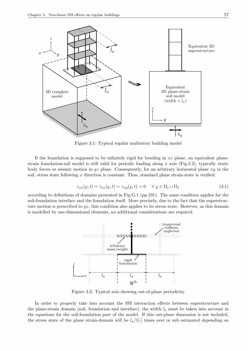
Chapter 3. Non-linear SSI effects on regular buildings 57
3D completemodel
la
la
ug
x y
z
Equivalent2D plane-strain
soil model(width = la)
Equivalent 2Dsuperstructure
ug
z
y
Figure 3.1: Typical regular multistory building model
If the foundation is supposed to be infinitely rigid for bending in xz plane, an equivalent plane-strain foundation-soil model is still valid for periodic loading along x axis (Fig.3.2), typically staticbody forces or seismic motion in yz plane. Consequently, for an arbitrary horizontal plane xy in thesoil, stress state following x direction is constant. Thus, standard plane strain-state is verified:
εxx(x, t) = γxz(x, t) = γxy(x, t) = 0 ∀ x ∈ Ωs ∪ Ωf (3.1)
according to definitions of domains presented in Fig.G.1 (pp.191). The same condition applies for thesoil-foundation interface and the foundation itself. More precisely, due to the fact that the superstruc-ture motion is prescribed to yz, this condition also applies to its stress state. However, as this domainis modelled by one-dimensional elements, no additional considerations are required.
la lala
tributarymass/weight
transversalstiffnessneglected
rigidfoundation
×ui
x
z
Figure 3.2: Typical axis showing out-of-plane periodicity
In order to properly take into account the SSI interaction effects between superstructure andthe plane-strain domain (soil, foundation and interface), the width la must be taken into account inthe equations for the soil-foundation part of the model. If this out-plane dimension is not included,the stress state of the plane strain-domain will be la/1[-] times over or sub estimated depending on

58 3.2. Modified plane-strain approach
the numeric value of la compared to traditional unit length plane-strain formulation. This effect isnot important for the linear elastic case, but under non-linear material assumption, neglecting thiscorrection can considerably alter the soil behavior and thus the obtained response.
The variational formulation presented in §1.2.4 is still valid. We repeat here the expression (1.39)for the superstructure domain Ωb for convenience:
∫
Ωb
σb: ε
b(wb) dV +
∫
Ωb
ρbub.wbdV =
∫
Ωb
ρb g.wbdV +
∫
Σbf
tb.wbdS +
∫
Γbσ
tb.wbdS (3.2)
It can be noticed that the soil-structure interface Σbs in Eq.1.39 has been changed by structure-foundation interface Σbf . In the foundation domain Ωf , integration of the weak formulation over thedomain must take into account the width la. In the previous expression, Ωb corresponds to a 3Ddomain, even if it is constituted by one-dimensional elements. The corresponding weak formulationfor the foundation domain can be written as:
la
∫
Ωf
ρf uf .wfdS = la
∫
Ωf
ρf g.wfdS +
∫
Σbf
t.wfdl + la
∫
Σf
t.wsfdl (3.3)
In (3.3), foundation domain is assumed rigid along x direction and one-phase. The correction factorla appears in the volumetric integration of inertial and body forces. On the soil-foundation interface,the width la must be also included. Free field condition is assumed over Γfσ
boundary. The modifiedweak-formulation for the soil domain is given by the following momentum conservation equation:
la
∫
Ωs
ρ us.ws dS + la
∫
Ωs
σ′s
: εs(ws) dS
−la∫
Ωs
p.div (ws) dS = la
∫
Ωs
ρ g.wsdS +
la
∫
Γsσ
t.wsdl + la
∫
Σsf
t.wsdl (3.4)
and the mass conservation:
− la∫
Ωs
ρf div(K.us
).q dS + la
∫
Ωs
div us.q dS
+la
∫
Ωs
p
Q.q dS + la
∫
Ωs
(K.grad p
).grad q dS = la
∫
Γϕ
ϕ∗.q dl
−la∫
Ωs
(K.grad
(ρfg.x
)).grad q dS
(3.5)
where the width la is included. The integration over Γsσ must be conducted carefully for the partcorresponding to soil domain truncation. As discussed in the previous chapter, in a part of thisboundary, dynamic conditions are used to ensure radiation condition and impose incident motion(paraxial elements described in §1.2.3). The equilibrium equation of the global system is obtainedby the addition of equations (3.2), (3.3) and (3.4), where discontinuity of displacements betweenfoundation and soil are introduced.
Assembling procedure, mesh partitions and resolution schema remain unchanged. These modifica-tions have been implemented and tested in GEFDyn code for solid 2D, interface and paraxial elements.Validations comparing results obtained by this approach with full 3D computations are described inthe following sections. These validations have been also used to define some properties for the modelsdescribed below, more precisely, the required stiffness for the shallow foundation to ensure the validityof plane-strain approach presented in this section.

Chapter 3. Non-linear SSI effects on regular buildings 59
3.3 Proposed approaches
In order to investigate the effect of non-linear soil behavior on seismic demand evaluation, a compar-ative dynamical analysis is carried out:
1. A complete finite element model including soil and structural non-linear behavior is used to assesthe effect of non-linear dynamic soil-structure interaction on the structural response (SSI-FE).
2. A two-step approach (T-S) is carried out in which:
(a) A non-linear 1D wave propagation problem is solved for a simple soil column of the foun-dation soil.
(b) The obtained free field motion is imposed as ground motion to a fixed base structural model.
The two approaches are presented schematically in Fig.3.3. SSI-FE takes into accounts all materialnon-linearities of soil, superstructure and interface, associated to seismic soil-structure interactionproblem. T-S approach takes into account non-linear behavior of soil and superstructure, but neglectsall interaction effects. This comparative approach was developed in order to provide two groups ofconsistent responses. The simple comparison of the SSI-FE approach with the fixed base responseimposing outcropping bedrock input motion is not adequate, because site effects will be neglected. Itis well known that modifications of the input motion due to soil conditions play a decisive role on thedynamic response of the superstructure.
SSI-FEproblem
1D wavepropagation
problemfixed baseproblem
Outcropping
t
aout(t)
Dec
onvol
ution
Bedrock
t
abed(t)
Free field
t
aff (t)
Figure 3.3: Proposed approaches
T-S approach corresponds to the state of the practice in earthquake engineering. In this work,wave propagation part of the T-S approach is achieved using the elastoplastic soil constitutive modelpresented in Appendix E. However, this step can be performed through the widely used equivalent-liner approach (Schnabel et al., 1972), or by employing 1D constitutive models (Mellal, 1997; Modaressiand Foerster, 2000) among others. The computed free field response can be injected later as input forany commercial non-linear structural dynamic code. On the contrary, a complete non-linear dynamicsoil-structure interaction is still out of the today’s engineering practice. Nevertheless, some simplifiedmethods for taking into account the nonlinear soil behavior in the DSSI problem through an equivalent
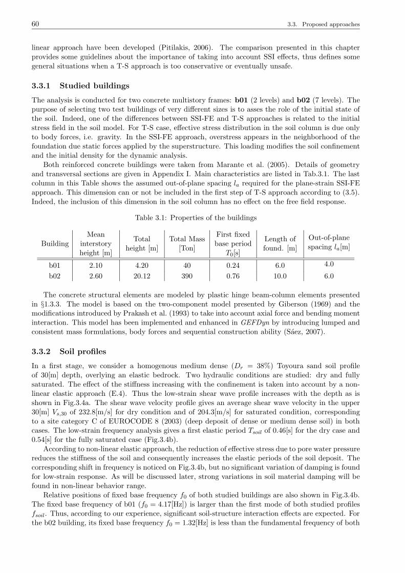
60 3.3. Proposed approaches
linear approach have been developed (Pitilakis, 2006). The comparison presented in this chapterprovides some guidelines about the importance of taking into account SSI effects, thus defines somegeneral situations when a T-S approach is too conservative or eventually unsafe.
3.3.1 Studied buildings
The analysis is conducted for two concrete multistory frames: b01 (2 levels) and b02 (7 levels). Thepurpose of selecting two test buildings of very different sizes is to asses the role of the initial state ofthe soil. Indeed, one of the differences between SSI-FE and T-S approaches is related to the initialstress field in the soil model. For T-S case, effective stress distribution in the soil column is due onlyto body forces, i.e. gravity. In the SSI-FE approach, overstress appears in the neighborhood of thefoundation due static forces applied by the superstructure. This loading modifies the soil confinementand the initial density for the dynamic analysis.
Both reinforced concrete buildings were taken from Marante et al. (2005). Details of geometryand transversal sections are given in Appendix I. Main characteristics are listed in Tab.3.1. The lastcolumn in this Table shows the assumed out-of-plane spacing la required for the plane-strain SSI-FEapproach. This dimension can or not be included in the first step of T-S approach according to (3.5).Indeed, the inclusion of this dimension in the soil column has no effect on the free field response.
Table 3.1: Properties of the buildings
BuildingMean
interstoryheight [m]
Totalheight [m]
Total Mass[Ton]
First fixedbase period
T0[s]
Length offound. [m]
Out-of-planespacing la[m]
b01 2.10 4.20 40 0.24 6.0 4.0
b02 2.60 20.12 390 0.76 10.0 6.0
The concrete structural elements are modeled by plastic hinge beam-column elements presentedin §1.3.3. The model is based on the two-component model presented by Giberson (1969) and themodifications introduced by Prakash et al. (1993) to take into account axial force and bending momentinteraction. This model has been implemented and enhanced in GEFDyn by introducing lumped andconsistent mass formulations, body forces and sequential construction ability (Saez, 2007).
3.3.2 Soil profiles
In a first stage, we consider a homogenous medium dense (Dr = 38%) Toyoura sand soil profileof 30[m] depth, overlying an elastic bedrock. Two hydraulic conditions are studied: dry and fullysaturated. The effect of the stiffness increasing with the confinement is taken into account by a non-linear elastic approach (E.4). Thus the low-strain shear wave profile increases with the depth as isshown in Fig.3.4a. The shear wave velocity profile gives an average shear wave velocity in the upper30[m] Vs,30 of 232.8[m/s] for dry condition and of 204.3[m/s] for saturated condition, correspondingto a site category C of EUROCODE 8 (2003) (deep deposit of dense or medium dense soil) in bothcases. The low-strain frequency analysis gives a first elastic period Tsoil of 0.46[s] for the dry case and0.54[s] for the fully saturated case (Fig.3.4b).
According to non-linear elastic approach, the reduction of effective stress due to pore water pressurereduces the stiffness of the soil and consequently increases the elastic periods of the soil deposit. Thecorresponding shift in frequency is noticed on Fig.3.4b, but no significant variation of damping is foundfor low-strain response. As will be discussed later, strong variations in soil material damping will befound in non-linear behavior range.
Relative positions of fixed base frequency f0 of both studied buildings are also shown in Fig.3.4b.The fixed base frequency of b01 (f0 = 4.17[Hz]) is larger than the first mode of both studied profilesfsoil. Thus, according to our experience, significant soil-structure interaction effects are expected. Forthe b02 building, its fixed base frequency f0 = 1.32[Hz] is less than the fundamental frequency of both
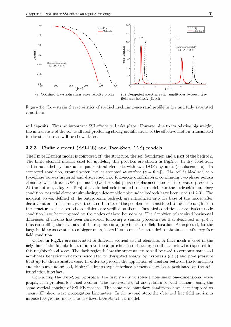
Chapter 3. Non-linear SSI effects on regular buildings 61
50 100 150 200 250 300−30
−25
−20
−15
−10
−5
0
Homogenous sandysoil (Dr = 38%)
Vs [m/s]
Dep
th [m
]
DrySaturated
(a) Obtained low-strain shear wave velocity profile
1 2 3 4 5 6 70
20
40
60
80
100
120
140
Homogenous sandysoil (Dr = 38%)
← b02 ← b01
f [Hz]
ff/bd
Mod
ulus
DrySaturated
(b) Computed spectral ratio amplitudes between freefield and bedrock (ff/bd)
Figure 3.4: Low-strain characteristics of studied medium dense sand profile in dry and fully saturatedconditions
soil deposits. Thus no important SSI effects will take place. However, due to its relative big weight,the initial state of the soil is altered producing strong modifications of the effective motion transmittedto the structure as will be shown later.
3.3.3 Finite element (SSI-FE) and Two-Step (T-S) models
The Finite Element model is composed of: the structure, the soil foundation and a part of the bedrock.The finite element meshes used for modeling this problem are shown in Fig.3.5. In dry condition,soil is modelled by four node quadrilateral elements with two DOFs by node (displacements). Insaturated condition, ground water level is assumed at surface (z = 0[m]). The soil is idealized as atwo-phase porous material and discretized into four-node quadrilateral continuum two-phase porouselements with three DOFs per node (two for solid phase displacement and one for water pressure).At the bottom, a layer of 5[m] of elastic bedrock is added to the model. For the bedrock’s boundarycondition, paraxial elements simulating a deformable unbounded bedrock have been used (§1.2.3). Theincident waves, defined at the outcropping bedrock are introduced into the base of the model afterdeconvolution. In the analysis, the lateral limits of the problem are considered to be far enough fromthe structure so that periodic conditions are verified on them. Thus, tied conditions or equivalent nodecondition have been imposed on the nodes of these boundaries. The definition of required horizontaldimension of meshes has been carried-out following a similar procedure as that described in §1.4.3,thus controlling the cleanness of the response at approximate free field location. As expected, for thelarge building associated to a bigger mass, lateral limits must be extended to obtain a satisfactory freefield condition.
Colors in Fig.3.5 are associated to different vertical size of elements. A finer mesh is used in theneighbor of the foundation to improve the approximation of strong non-linear behavior expected forthis neighborhood zone. The dark region below the superstructure will be used to compute some soilnon-linear behavior indicators associated to dissipated energy by hysteresis (§3.8) and pore pressurebuilt up for the saturated case. In order to prevent the apparition of traction between the foundationand the surrounding soil, Mohr-Coulombs type interface elements have been positioned at the soil-foundation interface.
Concerning the Two-Step approach, the first step is to solve a non-linear one-dimensional wavepropagation problem for a soil column. The mesh consists of one column of solid elements using thesame vertical spacing of SSI-FE meshes. The same tied boundary conditions have been imposed toensure 1D shear wave propagation kinematics. In the second step, the obtained free field motion isimposed as ground motion to the fixed base structural model.
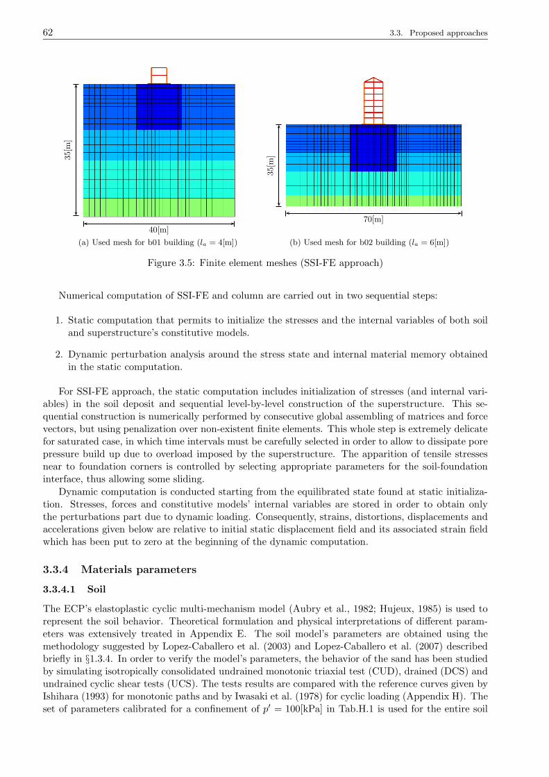
62 3.3. Proposed approaches
40[m]
35[m
]
(a) Used mesh for b01 building (la = 4[m])
70[m]
35[m
]
(b) Used mesh for b02 building (la = 6[m])
Figure 3.5: Finite element meshes (SSI-FE approach)
Numerical computation of SSI-FE and column are carried out in two sequential steps:
1. Static computation that permits to initialize the stresses and the internal variables of both soiland superstructure’s constitutive models.
2. Dynamic perturbation analysis around the stress state and internal material memory obtainedin the static computation.
For SSI-FE approach, the static computation includes initialization of stresses (and internal vari-ables) in the soil deposit and sequential level-by-level construction of the superstructure. This se-quential construction is numerically performed by consecutive global assembling of matrices and forcevectors, but using penalization over non-existent finite elements. This whole step is extremely delicatefor saturated case, in which time intervals must be carefully selected in order to allow to dissipate porepressure build up due to overload imposed by the superstructure. The apparition of tensile stressesnear to foundation corners is controlled by selecting appropriate parameters for the soil-foundationinterface, thus allowing some sliding.
Dynamic computation is conducted starting from the equilibrated state found at static initializa-tion. Stresses, forces and constitutive models’ internal variables are stored in order to obtain onlythe perturbations part due to dynamic loading. Consequently, strains, distortions, displacements andaccelerations given below are relative to initial static displacement field and its associated strain fieldwhich has been put to zero at the beginning of the dynamic computation.
3.3.4 Materials parameters
3.3.4.1 Soil
The ECP’s elastoplastic cyclic multi-mechanism model (Aubry et al., 1982; Hujeux, 1985) is used torepresent the soil behavior. Theoretical formulation and physical interpretations of different param-eters was extensively treated in Appendix E. The soil model’s parameters are obtained using themethodology suggested by Lopez-Caballero et al. (2003) and Lopez-Caballero et al. (2007) describedbriefly in §1.3.4. In order to verify the model’s parameters, the behavior of the sand has been studiedby simulating isotropically consolidated undrained monotonic triaxial test (CUD), drained (DCS) andundrained cyclic shear tests (UCS). The tests results are compared with the reference curves given byIshihara (1993) for monotonic paths and by Iwasaki et al. (1978) for cyclic loading (Appendix H). Theset of parameters calibrated for a confinement of p′ = 100[kPa] in Tab.H.1 is used for the entire soil
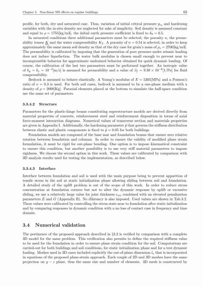
Chapter 3. Non-linear SSI effects on regular buildings 63
profile, for both, dry and saturated case. Thus, variation of initial critical pressure pc0 and hardeningvariables with the in-situ density are neglected for sake of simplicity. Soil density is assumed constantand equal to ρ = 1755[kg/m3], the initial earth pressure coefficient is fixed to k0 = 0.5.
In saturated conditions three additional parameters must be selected, the porosity n, the perme-ability tensor K and the water compressibility Kf . A porosity of n = 0.54 is selected, in order to keepapproximately the same mean soil density as that of the dry case for grain’s mass of ρs = 2700[kg/m3].The permeability is calibrated by imposing that the generation of pore pressure under seismic loadingdoes not induce liquefaction. The water bulk modulus is chosen small enough to prevent near toincompressible behavior for approximate undrained behavior obtained for quick dynamic loading. Ofcourse, the calibration of the last two parameters must be performed together. An isotropic valueof ky = kz = 10−4[m/s] is assumed for permeability and a value of βf = 9.38 × 10⁻⁸[1/Pa] for fluidcompressibility.
Bedrock is assumed to behave elastically. A Young’s modulus of E = 5305[MPa] and a Poisson’sratio of ν = 0.3 is used. For both soil cases, bedrock is assumed to be a one-phase medium with adensity of ρ = 2000[Kg]. Paraxial elements placed at the bottom to simulate the half-space conditionuse the same set of parameters.
3.3.4.2 Structure
Parameters for the plastic-hinge beams constituting superstructure models are derived directly frommaterial properties of concrete, reinforcement steel and reinforcement disposition in terms of axialforce-moment interaction diagrams. Numerical values of transverse section and materials propertiesare given in Appendix I. Additionally, the hardening parameter p that governs the stiffness distributionbetween elastic and plastic components is fixed to p = 0.05 for both buildings.
Foundation models are composed of the base mat and foundation beams that ensure zero relativerotation between foundation and columns. In order to ensure the validity of modified plane strainformulation, it must be rigid for out-plane bending. One option is to impose kinematical constraintto ensure this condition, but another possibility is to use very stiff material parameters to imposerigidness. We choose the second option in this work. These values are calibrated by comparison with3D analysis results used for testing the implementation, as described below.
3.3.4.3 Interface
Interface between foundation and soil is used with the main purpose being to prevent apparition oftensile stress in the soil at static initialization phase allowing sliding between soil and foundation.A detailed study of the uplift problem is out of the scope of this work. In order to reduce stressconcentration at foundation corners but not to alter the dynamic response by uplift or excessivesliding, we use a relatively large value for joint thickness eini combined with an elevated penalizationparameters E and G (Appendix B). No dilatancy is also imposed. Used values are shown in Tab.3.2.These values were calibrated by controlling the stress state near to foundation after static initializationand by comparing responses in dynamic condition with a no loss of contact case in frequency and timedomain.
3.4 Numerical validation
The pertinence of the proposed approach described in §3.2 is verified by comparison with a complete3D model for the same problem. This verification also permits to define the required stiffness valueto be used for the foundation in order to ensure plane strain condition for the soil. Computations arecarried-out for both buildings and soil conditions, for static initialization phase and for a test dynamicloading. Meshes used in 3D cases included explicitly the out-of-plane dimension la that is incorporatedin equations of the proposed plane-strain approach. Each couple of 2D and 3D meshes have the sameprojection on y − z plane, thus the same size and number of elements. 3D mesh is constructed by
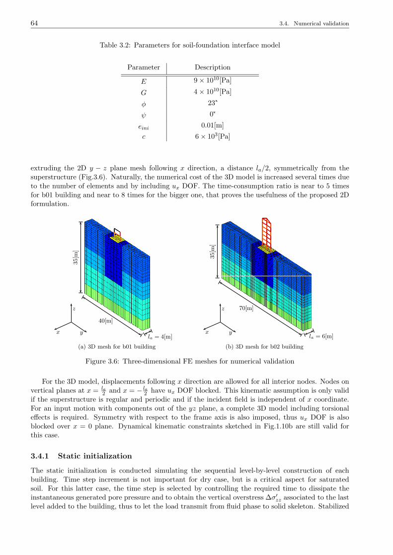
64 3.4. Numerical validation
Table 3.2: Parameters for soil-foundation interface model
Parameter Description
E 9× 10¹⁰[Pa]
G 4× 10¹⁰[Pa]
φ 23°ψ 0°eini 0.01[m]
c 6× 10³[Pa]
extruding the 2D y − z plane mesh following x direction, a distance la/2, symmetrically from thesuperstructure (Fig.3.6). Naturally, the numerical cost of the 3D model is increased several times dueto the number of elements and by including ux DOF. The time-consumption ratio is near to 5 timesfor b01 building and near to 8 times for the bigger one, that proves the usefulness of the proposed 2Dformulation.
40[m]
35[m
]
la = 4[m]
z
yx
(a) 3D mesh for b01 building
70[m]
35[m
]
la = 6[m]
z
yx
(b) 3D mesh for b02 building
Figure 3.6: Three-dimensional FE meshes for numerical validation
For the 3D model, displacements following x direction are allowed for all interior nodes. Nodes onvertical planes at x = la
2 and x = − la2 have ux DOF blocked. This kinematic assumption is only valid
if the superstructure is regular and periodic and if the incident field is independent of x coordinate.For an input motion with components out of the yz plane, a complete 3D model including torsionaleffects is required. Symmetry with respect to the frame axis is also imposed, thus ux DOF is alsoblocked over x = 0 plane. Dynamical kinematic constraints sketched in Fig.1.10b are still valid forthis case.
3.4.1 Static initialization
The static initialization is conducted simulating the sequential level-by-level construction of eachbuilding. Time step increment is not important for dry case, but is a critical aspect for saturatedsoil. For this latter case, the time step is selected by controlling the required time to dissipate theinstantaneous generated pore pressure and to obtain the vertical overstress ∆σ′zz associated to the lastlevel added to the building, thus to let the load transmit from fluid phase to solid skeleton. Stabilized
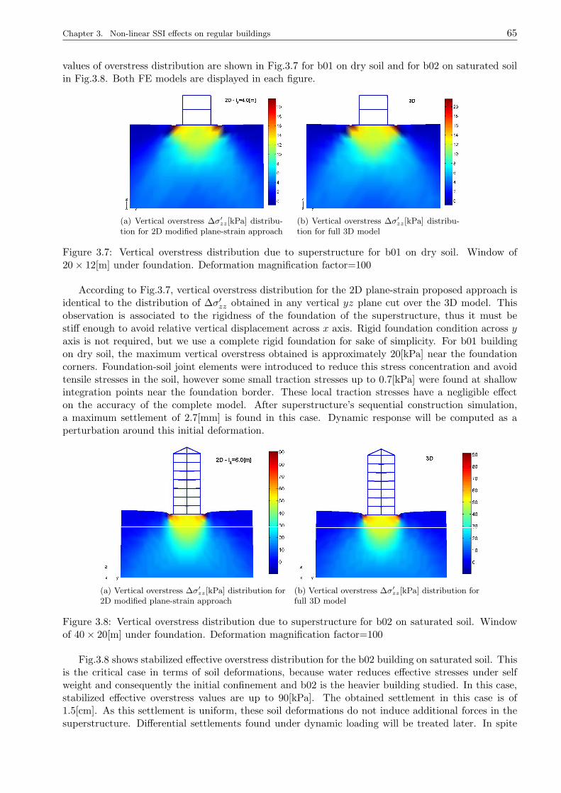
Chapter 3. Non-linear SSI effects on regular buildings 65
values of overstress distribution are shown in Fig.3.7 for b01 on dry soil and for b02 on saturated soilin Fig.3.8. Both FE models are displayed in each figure.
(a) Vertical overstress ∆σ′
zz[kPa] distribu-tion for 2D modified plane-strain approach
(b) Vertical overstress ∆σ′
zz[kPa] distribu-tion for full 3D model
Figure 3.7: Vertical overstress distribution due to superstructure for b01 on dry soil. Window of20× 12[m] under foundation. Deformation magnification factor=100
According to Fig.3.7, vertical overstress distribution for the 2D plane-strain proposed approach isidentical to the distribution of ∆σ′zz obtained in any vertical yz plane cut over the 3D model. Thisobservation is associated to the rigidness of the foundation of the superstructure, thus it must bestiff enough to avoid relative vertical displacement across x axis. Rigid foundation condition across yaxis is not required, but we use a complete rigid foundation for sake of simplicity. For b01 buildingon dry soil, the maximum vertical overstress obtained is approximately 20[kPa] near the foundationcorners. Foundation-soil joint elements were introduced to reduce this stress concentration and avoidtensile stresses in the soil, however some small traction stresses up to 0.7[kPa] were found at shallowintegration points near the foundation border. These local traction stresses have a negligible effecton the accuracy of the complete model. After superstructure’s sequential construction simulation,a maximum settlement of 2.7[mm] is found in this case. Dynamic response will be computed as aperturbation around this initial deformation.
(a) Vertical overstress ∆σ′
zz[kPa] distribution for2D modified plane-strain approach
(b) Vertical overstress ∆σ′
zz[kPa] distribution forfull 3D model
Figure 3.8: Vertical overstress distribution due to superstructure for b02 on saturated soil. Windowof 40× 20[m] under foundation. Deformation magnification factor=100
Fig.3.8 shows stabilized effective overstress distribution for the b02 building on saturated soil. Thisis the critical case in terms of soil deformations, because water reduces effective stresses under selfweight and consequently the initial confinement and b02 is the heavier building studied. In this case,stabilized effective overstress values are up to 90[kPa]. The obtained settlement in this case is of1.5[cm]. As this settlement is uniform, these soil deformations do not induce additional forces in thesuperstructure. Differential settlements found under dynamic loading will be treated later. In spite
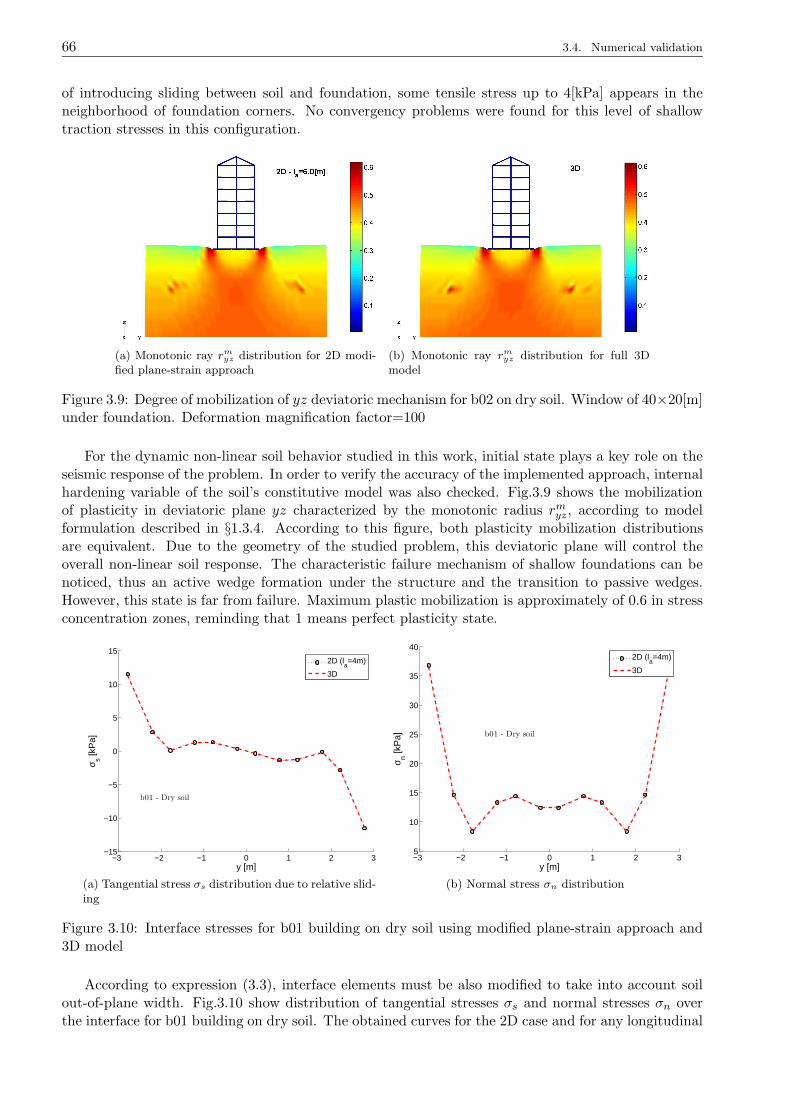
66 3.4. Numerical validation
of introducing sliding between soil and foundation, some tensile stress up to 4[kPa] appears in theneighborhood of foundation corners. No convergency problems were found for this level of shallowtraction stresses in this configuration.
(a) Monotonic ray rmyz distribution for 2D modi-
fied plane-strain approach(b) Monotonic ray rm
yz distribution for full 3Dmodel
Figure 3.9: Degree of mobilization of yz deviatoric mechanism for b02 on dry soil. Window of 40×20[m]under foundation. Deformation magnification factor=100
For the dynamic non-linear soil behavior studied in this work, initial state plays a key role on theseismic response of the problem. In order to verify the accuracy of the implemented approach, internalhardening variable of the soil’s constitutive model was also checked. Fig.3.9 shows the mobilizationof plasticity in deviatoric plane yz characterized by the monotonic radius rmyz, according to modelformulation described in §1.3.4. According to this figure, both plasticity mobilization distributionsare equivalent. Due to the geometry of the studied problem, this deviatoric plane will control theoverall non-linear soil response. The characteristic failure mechanism of shallow foundations can benoticed, thus an active wedge formation under the structure and the transition to passive wedges.However, this state is far from failure. Maximum plastic mobilization is approximately of 0.6 in stressconcentration zones, reminding that 1 means perfect plasticity state.
−3 −2 −1 0 1 2 3−15
−10
−5
0
5
10
15
b01 - Dry soil
y [m]
σ s [kP
a]
2D (la=4m)
3D
(a) Tangential stress σs distribution due to relative slid-ing
−3 −2 −1 0 1 2 35
10
15
20
25
30
35
40
b01 - Dry soil
y [m]
σ n [kP
a]
2D (la=4m)
3D
(b) Normal stress σn distribution
Figure 3.10: Interface stresses for b01 building on dry soil using modified plane-strain approach and3D model
According to expression (3.3), interface elements must be also modified to take into account soilout-of-plane width. Fig.3.10 show distribution of tangential stresses σs and normal stresses σn overthe interface for b01 building on dry soil. The obtained curves for the 2D case and for any longitudinal
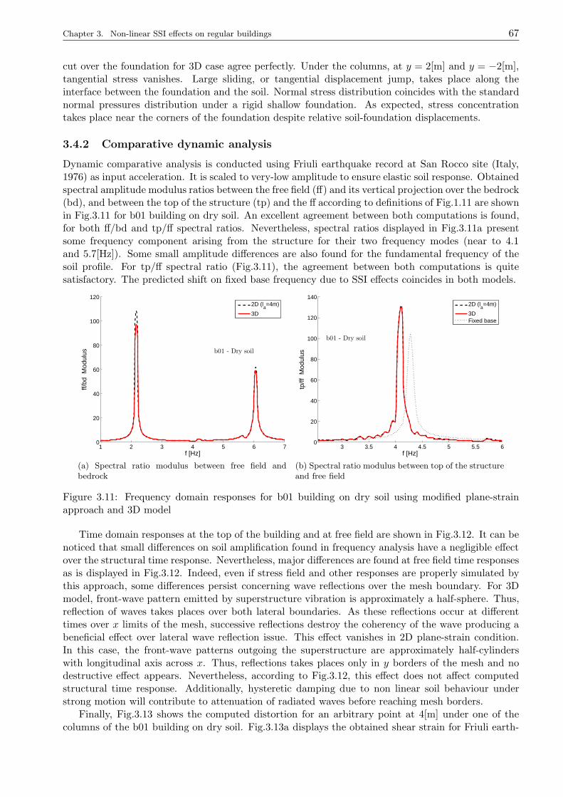
Chapter 3. Non-linear SSI effects on regular buildings 67
cut over the foundation for 3D case agree perfectly. Under the columns, at y = 2[m] and y = −2[m],tangential stress vanishes. Large sliding, or tangential displacement jump, takes place along theinterface between the foundation and the soil. Normal stress distribution coincides with the standardnormal pressures distribution under a rigid shallow foundation. As expected, stress concentrationtakes place near the corners of the foundation despite relative soil-foundation displacements.
3.4.2 Comparative dynamic analysis
Dynamic comparative analysis is conducted using Friuli earthquake record at San Rocco site (Italy,1976) as input acceleration. It is scaled to very-low amplitude to ensure elastic soil response. Obtainedspectral amplitude modulus ratios between the free field (ff) and its vertical projection over the bedrock(bd), and between the top of the structure (tp) and the ff according to definitions of Fig.1.11 are shownin Fig.3.11 for b01 building on dry soil. An excellent agreement between both computations is found,for both ff/bd and tp/ff spectral ratios. Nevertheless, spectral ratios displayed in Fig.3.11a presentsome frequency component arising from the structure for their two frequency modes (near to 4.1and 5.7[Hz]). Some small amplitude differences are also found for the fundamental frequency of thesoil profile. For tp/ff spectral ratio (Fig.3.11), the agreement between both computations is quitesatisfactory. The predicted shift on fixed base frequency due to SSI effects coincides in both models.
1 2 3 4 5 6 70
20
40
60
80
100
120
b01 - Dry soil
f [Hz]
ff/bd
Mod
ulus
2D (la=4m)
3D
(a) Spectral ratio modulus between free field andbedrock
3 3.5 4 4.5 5 5.5 60
20
40
60
80
100
120
140
b01 - Dry soil
f [Hz]
tp/ff
Mod
ulus
2D (la=4m)
3DFixed base
(b) Spectral ratio modulus between top of the structureand free field
Figure 3.11: Frequency domain responses for b01 building on dry soil using modified plane-strainapproach and 3D model
Time domain responses at the top of the building and at free field are shown in Fig.3.12. It can benoticed that small differences on soil amplification found in frequency analysis have a negligible effectover the structural time response. Nevertheless, major differences are found at free field time responsesas is displayed in Fig.3.12. Indeed, even if stress field and other responses are properly simulated bythis approach, some differences persist concerning wave reflections over the mesh boundary. For 3Dmodel, front-wave pattern emitted by superstructure vibration is approximately a half-sphere. Thus,reflection of waves takes places over both lateral boundaries. As these reflections occur at differenttimes over x limits of the mesh, successive reflections destroy the coherency of the wave producing abeneficial effect over lateral wave reflection issue. This effect vanishes in 2D plane-strain condition.In this case, the front-wave patterns outgoing the superstructure are approximately half-cylinderswith longitudinal axis across x. Thus, reflections takes places only in y borders of the mesh and nodestructive effect appears. Nevertheless, according to Fig.3.12, this effect does not affect computedstructural time response. Additionally, hysteretic damping due to non linear soil behaviour understrong motion will contribute to attenuation of radiated waves before reaching mesh borders.
Finally, Fig.3.13 shows the computed distortion for an arbitrary point at 4[m] under one of thecolumns of the b01 building on dry soil. Fig.3.13a displays the obtained shear strain for Friuli earth-
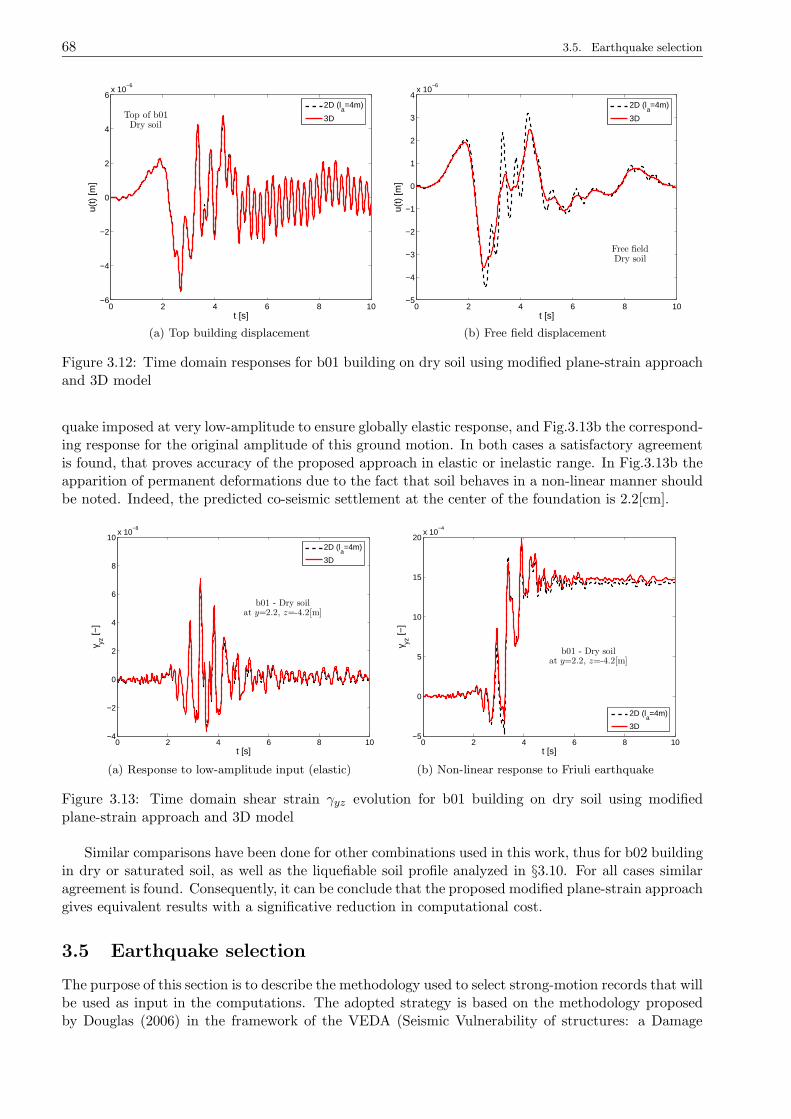
68 3.5. Earthquake selection
0 2 4 6 8 10−6
−4
−2
0
2
4
6x 10
−6
Top of b01Dry soil
t [s]
u(t)
[m]
2D (la=4m)
3D
(a) Top building displacement
0 2 4 6 8 10−5
−4
−3
−2
−1
0
1
2
3
4x 10
−6
Free fieldDry soil
t [s]
u(t)
[m]
2D (la=4m)
3D
(b) Free field displacement
Figure 3.12: Time domain responses for b01 building on dry soil using modified plane-strain approachand 3D model
quake imposed at very low-amplitude to ensure globally elastic response, and Fig.3.13b the correspond-ing response for the original amplitude of this ground motion. In both cases a satisfactory agreementis found, that proves accuracy of the proposed approach in elastic or inelastic range. In Fig.3.13b theapparition of permanent deformations due to the fact that soil behaves in a non-linear manner shouldbe noted. Indeed, the predicted co-seismic settlement at the center of the foundation is 2.2[cm].
0 2 4 6 8 10−4
−2
0
2
4
6
8
10x 10
−8
b01 - Dry soilat y=2.2, z=-4.2[m]
t [s]
γ yz [−
]
2D (la=4m)
3D
(a) Response to low-amplitude input (elastic)
0 2 4 6 8 10−5
0
5
10
15
20x 10
−4
b01 - Dry soilat y=2.2, z=-4.2[m]
t [s]
γ yz [−
]
2D (la=4m)
3D
(b) Non-linear response to Friuli earthquake
Figure 3.13: Time domain shear strain γyz evolution for b01 building on dry soil using modifiedplane-strain approach and 3D model
Similar comparisons have been done for other combinations used in this work, thus for b02 buildingin dry or saturated soil, as well as the liquefiable soil profile analyzed in §3.10. For all cases similaragreement is found. Consequently, it can be conclude that the proposed modified plane-strain approachgives equivalent results with a significative reduction in computational cost.
3.5 Earthquake selection
The purpose of this section is to describe the methodology used to select strong-motion records that willbe used as input in the computations. The adopted strategy is based on the methodology proposedby Douglas (2006) in the framework of the VEDA (Seismic Vulnerability of structures: a Damage
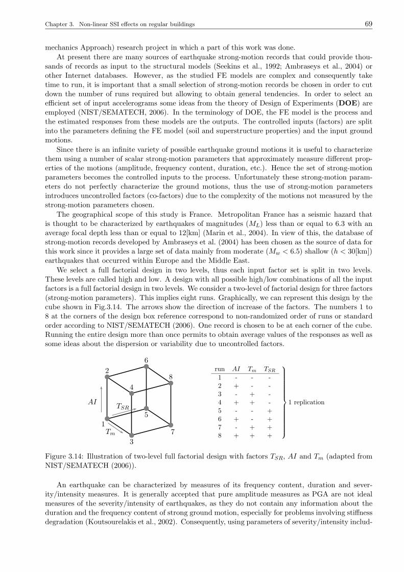
Chapter 3. Non-linear SSI effects on regular buildings 69
mechanics Approach) research project in which a part of this work was done.
At present there are many sources of earthquake strong-motion records that could provide thou-sands of records as input to the structural models (Seekins et al., 1992; Ambraseys et al., 2004) orother Internet databases. However, as the studied FE models are complex and consequently taketime to run, it is important that a small selection of strong-motion records be chosen in order to cutdown the number of runs required but allowing to obtain general tendencies. In order to select anefficient set of input accelerograms some ideas from the theory of Design of Experiments (DOE) areemployed (NIST/SEMATECH, 2006). In the terminology of DOE, the FE model is the process andthe estimated responses from these models are the outputs. The controlled inputs (factors) are splitinto the parameters defining the FE model (soil and superstructure properties) and the input groundmotions.
Since there is an infinite variety of possible earthquake ground motions it is useful to characterizethem using a number of scalar strong-motion parameters that approximately measure different prop-erties of the motions (amplitude, frequency content, duration, etc.). Hence the set of strong-motionparameters becomes the controlled inputs to the process. Unfortunately these strong-motion param-eters do not perfectly characterize the ground motions, thus the use of strong-motion parametersintroduces uncontrolled factors (co-factors) due to the complexity of the motions not measured by thestrong-motion parameters chosen.
The geographical scope of this study is France. Metropolitan France has a seismic hazard thatis thought to be characterized by earthquakes of magnitudes (ML) less than or equal to 6.3 with anaverage focal depth less than or equal to 12[km] (Marin et al., 2004). In view of this, the database ofstrong-motion records developed by Ambraseys et al. (2004) has been chosen as the source of data forthis work since it provides a large set of data mainly from moderate (Mw < 6.5) shallow (h < 30[km])earthquakes that occurred within Europe and the Middle East.
We select a full factorial design in two levels, thus each input factor set is split in two levels.These levels are called high and low. A design with all possible high/low combinations of all the inputfactors is a full factorial design in two levels. We consider a two-level of factorial design for three factors(strong-motion parameters). This implies eight runs. Graphically, we can represent this design by thecube shown in Fig.3.14. The arrows show the direction of increase of the factors. The numbers 1 to8 at the corners of the design box reference correspond to non-randomized order of runs or standardorder according to NIST/SEMATECH (2006). One record is chosen to be at each corner of the cube.Running the entire design more than once permits to obtain average values of the responses as well assome ideas about the dispersion or variability due to uncontrolled factors.
b1
b2
b3
b4
b5
b6
b
7
b8
Tm
TSRAI
run AI Tm TSR1 - - -2 + - -3 - + -4 + + -5 - - +6 + - +7 - + +8 + + +
1 replication
Figure 3.14: Illustration of two-level full factorial design with factors TSR, AI and Tm (adapted fromNIST/SEMATECH (2006)).
An earthquake can be characterized by measures of its frequency content, duration and sever-ity/intensity measures. It is generally accepted that pure amplitude measures as PGA are not idealmeasures of the severity/intensity of earthquakes, as they do not contain any information about theduration and the frequency content of strong ground motion, especially for problems involving stiffnessdegradation (Koutsourelakis et al., 2002). Consequently, using parameters of severity/intensity includ-
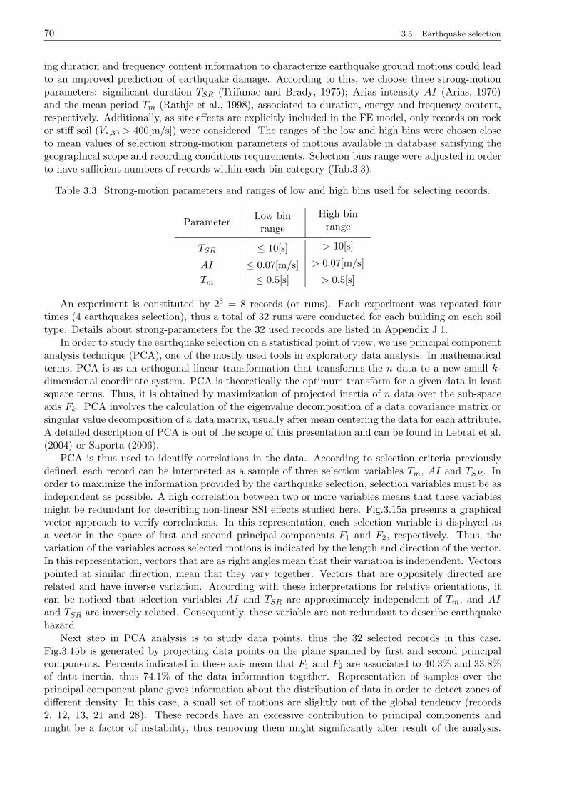
70 3.5. Earthquake selection
ing duration and frequency content information to characterize earthquake ground motions could leadto an improved prediction of earthquake damage. According to this, we choose three strong-motionparameters: significant duration TSR (Trifunac and Brady, 1975); Arias intensity AI (Arias, 1970)and the mean period Tm (Rathje et al., 1998), associated to duration, energy and frequency content,respectively. Additionally, as site effects are explicitly included in the FE model, only records on rockor stiff soil (Vs,30 > 400[m/s]) were considered. The ranges of the low and high bins were chosen closeto mean values of selection strong-motion parameters of motions available in database satisfying thegeographical scope and recording conditions requirements. Selection bins range were adjusted in orderto have sufficient numbers of records within each bin category (Tab.3.3).
Table 3.3: Strong-motion parameters and ranges of low and high bins used for selecting records.
ParameterLow binrange
High binrange
TSR ≤ 10[s] > 10[s]
AI ≤ 0.07[m/s] > 0.07[m/s]
Tm ≤ 0.5[s] > 0.5[s]
An experiment is constituted by 23 = 8 records (or runs). Each experiment was repeated fourtimes (4 earthquakes selection), thus a total of 32 runs were conducted for each building on each soiltype. Details about strong-parameters for the 32 used records are listed in Appendix J.1.
In order to study the earthquake selection on a statistical point of view, we use principal componentanalysis technique (PCA), one of the mostly used tools in exploratory data analysis. In mathematicalterms, PCA is as an orthogonal linear transformation that transforms the n data to a new small k-dimensional coordinate system. PCA is theoretically the optimum transform for a given data in leastsquare terms. Thus, it is obtained by maximization of projected inertia of n data over the sub-spaceaxis Fk. PCA involves the calculation of the eigenvalue decomposition of a data covariance matrix orsingular value decomposition of a data matrix, usually after mean centering the data for each attribute.A detailed description of PCA is out of the scope of this presentation and can be found in Lebrat et al.(2004) or Saporta (2006).
PCA is thus used to identify correlations in the data. According to selection criteria previouslydefined, each record can be interpreted as a sample of three selection variables Tm, AI and TSR. Inorder to maximize the information provided by the earthquake selection, selection variables must be asindependent as possible. A high correlation between two or more variables means that these variablesmight be redundant for describing non-linear SSI effects studied here. Fig.3.15a presents a graphicalvector approach to verify correlations. In this representation, each selection variable is displayed asa vector in the space of first and second principal components F1 and F2, respectively. Thus, thevariation of the variables across selected motions is indicated by the length and direction of the vector.In this representation, vectors that are as right angles mean that their variation is independent. Vectorspointed at similar direction, mean that they vary together. Vectors that are oppositely directed arerelated and have inverse variation. According with these interpretations for relative orientations, itcan be noticed that selection variables AI and TSR are approximately independent of Tm, and AIand TSR are inversely related. Consequently, these variable are not redundant to describe earthquakehazard.
Next step in PCA analysis is to study data points, thus the 32 selected records in this case.Fig.3.15b is generated by projecting data points on the plane spanned by first and second principalcomponents. Percents indicated in these axis mean that F1 and F2 are associated to 40.3% and 33.8%of data inertia, thus 74.1% of the data information together. Representation of samples over theprincipal component plane gives information about the distribution of data in order to detect zones ofdifferent density. In this case, a small set of motions are slightly out of the global tendency (records2, 12, 13, 21 and 28). These records have an excessive contribution to principal components andmight be a factor of instability, thus removing them might significantly alter result of the analysis.
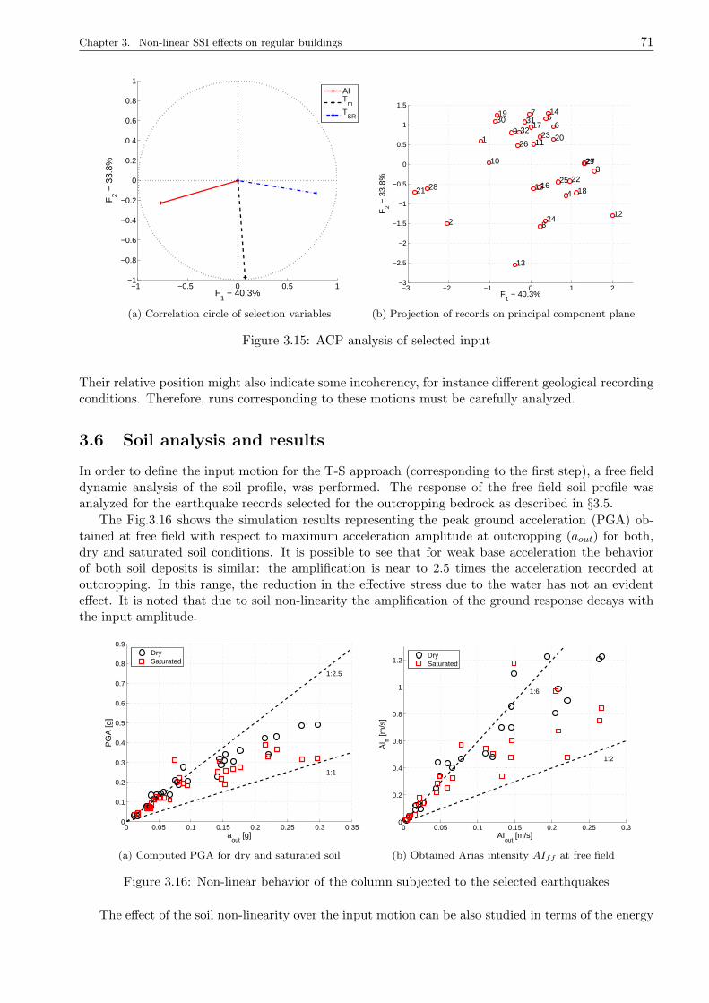
Chapter 3. Non-linear SSI effects on regular buildings 71
−1 −0.5 0 0.5 1−1
−0.8
−0.6
−0.4
−0.2
0
0.2
0.4
0.6
0.8
1
F1 − 40.3%
F2 −
33.
8%
AIT
mT
SR
(a) Correlation circle of selection variables
−3 −2 −1 0 1 2−3
−2.5
−2
−1.5
−1
−0.5
0
0.5
1
1.5
1
2
3
4
56
7
8
9
10
11
12
13
14
1516
17
18
19
20
2122
23
24
25
26
27
28
29
30 3132
F1 − 40.3%
F2 −
33.
8%
(b) Projection of records on principal component plane
Figure 3.15: ACP analysis of selected input
Their relative position might also indicate some incoherency, for instance different geological recordingconditions. Therefore, runs corresponding to these motions must be carefully analyzed.
3.6 Soil analysis and results
In order to define the input motion for the T-S approach (corresponding to the first step), a free fielddynamic analysis of the soil profile, was performed. The response of the free field soil profile wasanalyzed for the earthquake records selected for the outcropping bedrock as described in §3.5.
The Fig.3.16 shows the simulation results representing the peak ground acceleration (PGA) ob-tained at free field with respect to maximum acceleration amplitude at outcropping (aout) for both,dry and saturated soil conditions. It is possible to see that for weak base acceleration the behaviorof both soil deposits is similar: the amplification is near to 2.5 times the acceleration recorded atoutcropping. In this range, the reduction in the effective stress due to the water has not an evidenteffect. It is noted that due to soil non-linearity the amplification of the ground response decays withthe input amplitude.
0 0.05 0.1 0.15 0.2 0.25 0.3 0.350
0.1
0.2
0.3
0.4
0.5
0.6
0.7
0.8
0.9
1:1
1:2.5
aout
[g]
PG
A [g
]
DrySaturated
(a) Computed PGA for dry and saturated soil
0 0.05 0.1 0.15 0.2 0.25 0.30
0.2
0.4
0.6
0.8
1
1.2
1:2
1:6
AIout
[m/s]
AI ff [m
/s]
DrySaturated
(b) Obtained Arias intensity AIff at free field
Figure 3.16: Non-linear behavior of the column subjected to the selected earthquakes
The effect of the soil non-linearity over the input motion can be also studied in terms of the energy
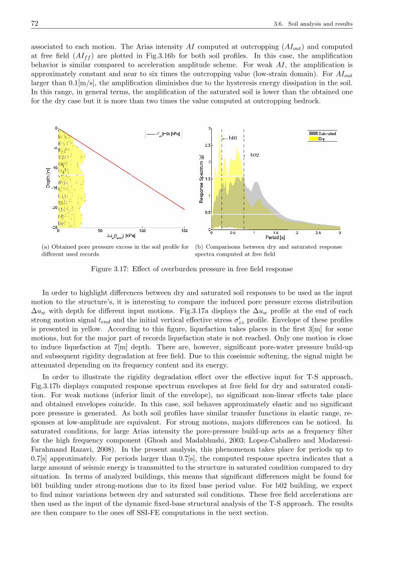
72 3.6. Soil analysis and results
associated to each motion. The Arias intensity AI computed at outcropping (AIout) and computedat free field (AIff ) are plotted in Fig.3.16b for both soil profiles. In this case, the amplificationbehavior is similar compared to acceleration amplitude scheme. For weak AI, the amplification isapproximately constant and near to six times the outcropping value (low-strain domain). For AIoutlarger than 0.1[m/s], the amplification diminishes due to the hysteresis energy dissipation in the soil.In this range, in general terms, the amplification of the saturated soil is lower than the obtained onefor the dry case but it is more than two times the value computed at outcropping bedrock.
(a) Obtained pore pressure excess in the soil profile fordifferent used records
(b) Comparisons between dry and saturated responsespectra computed at free field
Figure 3.17: Effect of overburden pressure in free field response
In order to highlight differences between dry and saturated soil responses to be used as the inputmotion to the structure’s, it is interesting to compare the induced pore pressure excess distribution∆uw with depth for different input motions. Fig.3.17a displays the ∆uw profile at the end of eachstrong motion signal tend and the initial vertical effective stress σ′zz profile. Envelope of these profilesis presented in yellow. According to this figure, liquefaction takes places in the first 3[m] for somemotions, but for the major part of records liquefaction state is not reached. Only one motion is closeto induce liquefaction at 7[m] depth. There are, however, significant pore-water pressure build-upand subsequent rigidity degradation at free field. Due to this coseismic softening, the signal might beattenuated depending on its frequency content and its energy.
In order to illustrate the rigidity degradation effect over the effective input for T-S approach,Fig.3.17b displays computed response spectrum envelopes at free field for dry and saturated condi-tion. For weak motions (inferior limit of the envelope), no significant non-linear effects take placeand obtained envelopes coincide. In this case, soil behaves approximately elastic and no significantpore pressure is generated. As both soil profiles have similar transfer functions in elastic range, re-sponses at low-amplitude are equivalent. For strong motions, majors differences can be noticed. Insaturated conditions, for large Arias intensity the pore-pressure build-up acts as a frequency filterfor the high frequency component (Ghosh and Madabhushi, 2003; Lopez-Caballero and Modaressi-Farahmand Razavi, 2008). In the present analysis, this phenomenon takes place for periods up to0.7[s] approximately. For periods larger than 0.7[s], the computed response spectra indicates that alarge amount of seismic energy is transmitted to the structure in saturated condition compared to drysituation. In terms of analyzed buildings, this means that significant differences might be found forb01 building under strong-motions due to its fixed base period value. For b02 building, we expectto find minor variations between dry and saturated soil conditions. These free field accelerations arethen used as the input of the dynamic fixed-base structural analysis of the T-S approach. The resultsare then compare to the ones off SSI-FE computations in the next section.

Chapter 3. Non-linear SSI effects on regular buildings 73
3.7 Effect of SSI on the dynamic response
The same set of input motions listed in Appendix J.1, are used in the SSI-FE simulations. In orderto assess the influence of the SSI effects on the dynamic non-linear structural response, the results ofthe two approaches for each building and for each soil are shown in Figures 3.18, 3.19, 3.22 and 3.23.Results are presented in the form of scatter plots of the maximum value of the computed inter-storydrift normalized by the corresponding inter-story height (ISDmax,%) for each record as a functionof the strong-motion parameters of the earthquakes. In order to use a common reference for bothT-S and SSI-FE approaches, severity measures computed at outcropping or free field might be usedfor these figures on the x-axis. In general, it is accepted that acceleration amplitude as the measureof severity of earthquakes is not ideal because it does not contain information about the durationand frequency content. This aspect is critical for systems involving stiffness degradation, where theduration and frequency content of strong motion have a profound effect on the response of the system(Koutsourelakis et al., 2002). Correlations between several strong-motion parameters and the observedresponses will be discussed in the following.
0 0.05 0.1 0.15 0.2 0.25 0.3 0.350
0.1
0.2
0.3
0.4
0.5
0.6
0.7
b01 - Dry soil
aout
[g]
ISD
max
%
SSI−FET−S
(a) Computed ISDmax,% in terms of outcrop accelera-tion amplitude aout
0 0.1 0.2 0.3 0.4 0.5 0.6 0.7 0.8 0.90
0.1
0.2
0.3
0.4
0.5
0.6
0.7
b01 - Dry soil
AIout
[m/s]
ISD
max
%
SSI−FET−S
(b) Obtained ISDmax,% in terms of outcrop Arias’s in-tensity AIout
Figure 3.18: Scatter plots of maximum inter-story drift for b01 building on dry soil
Figures 3.18a and 3.18b provide scatter plots of the maximum response of ISDmax% in terms ofaout and AIout, respectively, for the b01 building on dry soil. According to these figures in a generalway, including non-linear SSI effects in the dynamic computation reduces the obtained maximuminter-story drift. However, results present dispersion, thus for approximately the same value of inputseverity large variation of ISDmax,% is found. In order to define the more suitable strong-motionparameter to describe the computed seismic demand, correlation coefficients ρX,Y between ISDmax,%
and the maximum amplitude of the acceleration at outcropping bedrock (aout) and at free field (PGA),the Arias intensity at outcropping bedrock (AIout) and at free field (AIff ), the mean period Tm andthe predominant period of the ground motion Tg (Miranda and Vertero, 1994), for each studied caseare listed in Tab.3.4.
According to Tab.3.4, correlation coefficients between free field or outcropping bedrock severitymeasures are equivalent, thus corresponding ρX,Y values for aout compared to PGA or AIout comparedto AIff are similar. As computed values at outcropping bedrock depends only of the input motioncharacteristics, we select outcropping measures to simplify the interpretation of results. Consequently,hereinafter two alternative of measures are considered: the maximum amplitude of the accelerationat outcropping bedrock aout and the corresponding Arias intensity AIout. According to values of ρX,Ylisted in Tab.3.4 for aout and AIout, depending on the building and the soil considered, one of themmight be better than the other to describe the expected maximum structural response. Indeed, valuesof correlations coefficients are in general of the same order for both parameters. As a general rule,
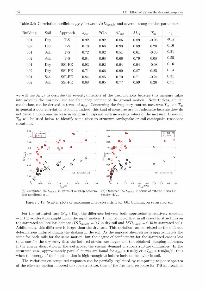
74 3.7. Effect of SSI on the dynamic response
Table 3.4: Correlation coefficient ρX,Y between ISDmax,% and several strong-motion parameters
Building Soil Approach aout PGA AIout AIff Tm Tg
b01 Dry T-S 0.92 0.92 0.86 0.89 -0.06 -0.17
b02 Dry T-S 0.73 0.68 0.93 0.89 0.20 0.16
b01 Sat. T-S 0.72 0.82 0.51 0.61 -0.30 0.21
b02 Sat. T-S 0.64 0.68 0.66 0.79 0.08 0.55
b01 Dry SSI-FE 0.93 0.92 0.94 0.94 -0.08 0.16
b02 Dry SSI-FE 0.71 0.66 0.90 0.87 0.25 0.14
b01 Sat. SSI-FE 0.84 0.85 0.70 0.71 -0.24 0.31
b02 Sat. SSI-FE 0.68 0.65 0.77 0.89 0.26 0.71
we will use AIout to describe the severity/intensity of the used motions because this measure takesinto account the duration and the frequency content of the ground motion. Nevertheless, similarconclusions can be derived in terms of aout. Concerning the frequency content measures Tm and Tg,in general a poor correlation is found. Indeed, this kind of measures are not adequate because they donot cause a monotonic increase in structural response with increasing values of the measure. However,Tm will be used below to identify some close to structure-earthquake or soil-earthquake resonancesituations.
0 0.05 0.1 0.15 0.2 0.25 0.3 0.350
0.05
0.1
0.15
0.2
0.25
0.3
0.35
0.4
0.45
b01 - Saturated soil
aout
[g]
ISD
max
%
SSI−FET−S
(a) Computed ISDmax,% in terms of outcrop accelera-tion amplitude aout
0 0.1 0.2 0.3 0.4 0.5 0.6 0.7 0.8 0.90
0.05
0.1
0.15
0.2
0.25
0.3
0.35
0.4
0.45
b01 - Saturated soil
AIout
[m/s]
ISD
max
%
SSI−FET−S
(b) Obtained ISDmax,% in terms of outcrop Arias’s in-tensity AIout
Figure 3.19: Scatter plots of maximum inter-story drift for b01 building on saturated soil
For the saturated case (Fig.3.19a), the difference between both approaches is relatively constantover the acceleration amplitude of the input motion. It can be noted that in all cases the structures onthe saturated soil are less damage (ISDmax% = 0.7 in dry soil and ISDmax% = 0.45 in saturated soil).Additionally, this difference is larger than the dry case. This variation can be related to the differentdeformations induced during the shaking in the soil. As the imposed shear stress is approximately thesame for both soils for the same motion, but the degree of confinement for the saturated case is lessthan one for the dry case, thus the induced strains are larger and the obtained damping increases.If the energy dissipation in the soil grows, the seismic demand of superstructure diminishes. In thesaturated case, approximately parallel curves are found for aout > 0.04[g] or AIout > 0.05[m/s], thuswhen the energy of the input motion is high enough to induce inelastic behavior in soil.
The variations on computed responses can be partially explained by computing response spectraof the effective motion imposed to superstructure, thus of the free field response for T-S approach or
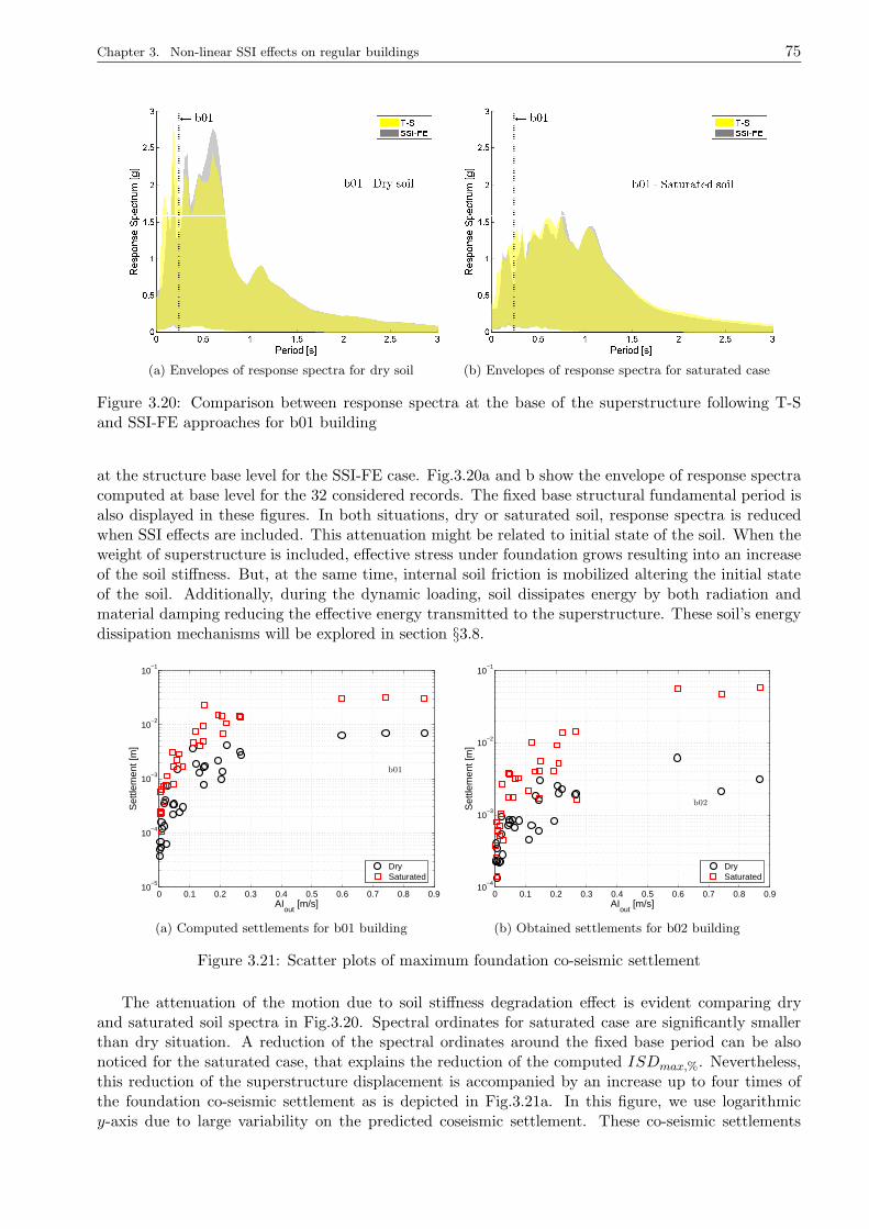
Chapter 3. Non-linear SSI effects on regular buildings 75
(a) Envelopes of response spectra for dry soil (b) Envelopes of response spectra for saturated case
Figure 3.20: Comparison between response spectra at the base of the superstructure following T-Sand SSI-FE approaches for b01 building
at the structure base level for the SSI-FE case. Fig.3.20a and b show the envelope of response spectracomputed at base level for the 32 considered records. The fixed base structural fundamental period isalso displayed in these figures. In both situations, dry or saturated soil, response spectra is reducedwhen SSI effects are included. This attenuation might be related to initial state of the soil. When theweight of superstructure is included, effective stress under foundation grows resulting into an increaseof the soil stiffness. But, at the same time, internal soil friction is mobilized altering the initial stateof the soil. Additionally, during the dynamic loading, soil dissipates energy by both radiation andmaterial damping reducing the effective energy transmitted to the superstructure. These soil’s energydissipation mechanisms will be explored in section §3.8.
0 0.1 0.2 0.3 0.4 0.5 0.6 0.7 0.8 0.910
−5
10−4
10−3
10−2
10−1
b01
AIout
[m/s]
Set
tlem
ent [
m]
DrySaturated
(a) Computed settlements for b01 building
0 0.1 0.2 0.3 0.4 0.5 0.6 0.7 0.8 0.910
−4
10−3
10−2
10−1
b02
AIout
[m/s]
Set
tlem
ent [
m]
DrySaturated
(b) Obtained settlements for b02 building
Figure 3.21: Scatter plots of maximum foundation co-seismic settlement
The attenuation of the motion due to soil stiffness degradation effect is evident comparing dryand saturated soil spectra in Fig.3.20. Spectral ordinates for saturated case are significantly smallerthan dry situation. A reduction of the spectral ordinates around the fixed base period can be alsonoticed for the saturated case, that explains the reduction of the computed ISDmax,%. Nevertheless,this reduction of the superstructure displacement is accompanied by an increase up to four times ofthe foundation co-seismic settlement as is depicted in Fig.3.21a. In this figure, we use logarithmicy-axis due to large variability on the predicted coseismic settlement. These co-seismic settlements
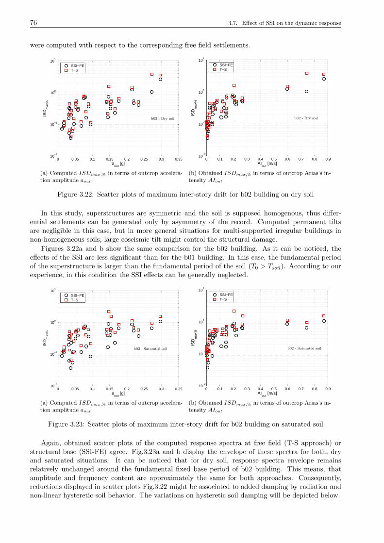
76 3.7. Effect of SSI on the dynamic response
were computed with respect to the corresponding free field settlements.
0 0.05 0.1 0.15 0.2 0.25 0.3 0.3510
−2
10−1
100
101
b02 - Dry soil
aout
[g]
ISD
max
%
SSI−FET−S
(a) Computed ISDmax,% in terms of outcrop accelera-tion amplitude aout
0 0.1 0.2 0.3 0.4 0.5 0.6 0.7 0.8 0.910
−2
10−1
100
101
b02 - Dry soil
AIout
[m/s]
ISD
max
%
SSI−FET−S
(b) Obtained ISDmax,% in terms of outcrop Arias’s in-tensity AIout
Figure 3.22: Scatter plots of maximum inter-story drift for b02 building on dry soil
In this study, superstructures are symmetric and the soil is supposed homogenous, thus differ-ential settlements can be generated only by asymmetry of the record. Computed permanent tiltsare negligible in this case, but in more general situations for multi-supported irregular buildings innon-homogeneous soils, large coseismic tilt might control the structural damage.
Figures 3.22a and b show the same comparison for the b02 building. As it can be noticed, theeffects of the SSI are less significant than for the b01 building. In this case, the fundamental periodof the superstructure is larger than the fundamental period of the soil (T0 > Tsoil). According to ourexperience, in this condition the SSI effects can be generally neglected.
0 0.05 0.1 0.15 0.2 0.25 0.3 0.3510
−2
10−1
100
101
b02 - Saturated soil
aout
[g]
ISD
max
%
SSI−FET−S
(a) Computed ISDmax,% in terms of outcrop accelera-tion amplitude aout
0 0.1 0.2 0.3 0.4 0.5 0.6 0.7 0.8 0.910
−2
10−1
100
101
b02 - Saturated soil
AIout
[m/s]
ISD
max
%
SSI−FET−S
(b) Obtained ISDmax,% in terms of outcrop Arias’s in-tensity AIout
Figure 3.23: Scatter plots of maximum inter-story drift for b02 building on saturated soil
Again, obtained scatter plots of the computed response spectra at free field (T-S approach) orstructural base (SSI-FE) agree. Fig.3.23a and b display the envelope of these spectra for both, dryand saturated situations. It can be noticed that for dry soil, response spectra envelope remainsrelatively unchanged around the fundamental fixed base period of b02 building. This means, thatamplitude and frequency content are approximately the same for both approaches. Consequently,reductions displayed in scatter plots Fig.3.22 might be associated to added damping by radiation andnon-linear hysteretic soil behavior. The variations on hysteretic soil damping will be depicted below.
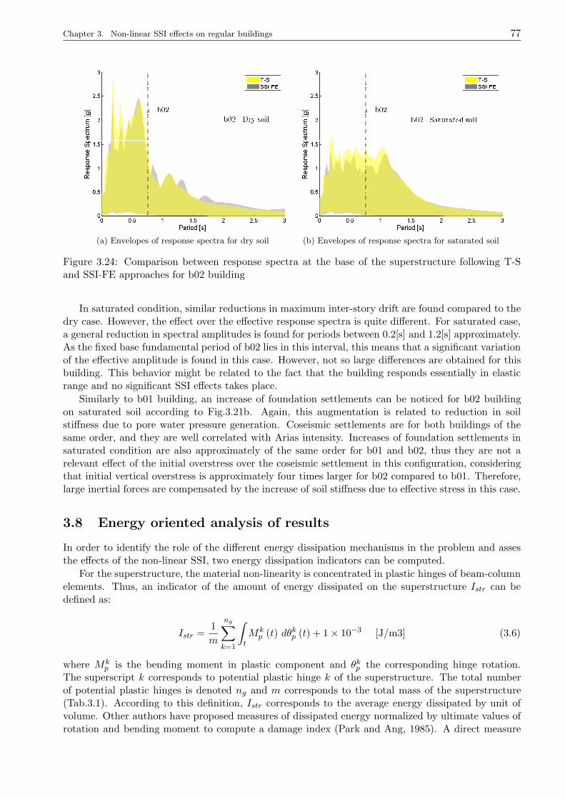
Chapter 3. Non-linear SSI effects on regular buildings 77
(a) Envelopes of response spectra for dry soil (b) Envelopes of response spectra for saturated soil
Figure 3.24: Comparison between response spectra at the base of the superstructure following T-Sand SSI-FE approaches for b02 building
In saturated condition, similar reductions in maximum inter-story drift are found compared to thedry case. However, the effect over the effective response spectra is quite different. For saturated case,a general reduction in spectral amplitudes is found for periods between 0.2[s] and 1.2[s] approximately.As the fixed base fundamental period of b02 lies in this interval, this means that a significant variationof the effective amplitude is found in this case. However, not so large differences are obtained for thisbuilding. This behavior might be related to the fact that the building responds essentially in elasticrange and no significant SSI effects takes place.
Similarly to b01 building, an increase of foundation settlements can be noticed for b02 buildingon saturated soil according to Fig.3.21b. Again, this augmentation is related to reduction in soilstiffness due to pore water pressure generation. Coseismic settlements are for both buildings of thesame order, and they are well correlated with Arias intensity. Increases of foundation settlements insaturated condition are also approximately of the same order for b01 and b02, thus they are not arelevant effect of the initial overstress over the coseismic settlement in this configuration, consideringthat initial vertical overstress is approximately four times larger for b02 compared to b01. Therefore,large inertial forces are compensated by the increase of soil stiffness due to effective stress in this case.
3.8 Energy oriented analysis of results
In order to identify the role of the different energy dissipation mechanisms in the problem and assesthe effects of the non-linear SSI, two energy dissipation indicators can be computed.
For the superstructure, the material non-linearity is concentrated in plastic hinges of beam-columnelements. Thus, an indicator of the amount of energy dissipated on the superstructure Istr can bedefined as:
Istr =1
m
ng∑
k=1
∫
t
Mkp (t) dθkp (t) + 1× 10⁻³ [J/m3] (3.6)
where Mkp is the bending moment in plastic component and θkp the corresponding hinge rotation.
The superscript k corresponds to potential plastic hinge k of the superstructure. The total numberof potential plastic hinges is denoted ng and m corresponds to the total mass of the superstructure(Tab.3.1). According to this definition, Istr corresponds to the average energy dissipated by unit ofvolume. Other authors have proposed measures of dissipated energy normalized by ultimate values ofrotation and bending moment to compute a damage index (Park and Ang, 1985). A direct measure
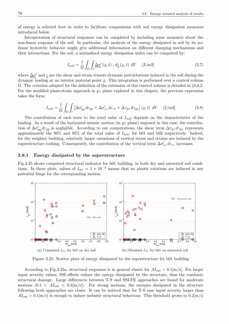
78 3.8. Energy oriented analysis of results
of energy is selected here in order to facilitate comparisons with soil energy dissipation measuresintroduced below.
Interpretation of structural responses can be completed by including some measures about thenon-linear response of the soil. In particular, the analysis of the energy dissipated in soil by its no-linear hysteretic behavior might give additional information on different damping mechanisms andtheir interactions. For the soil, a normalized energy dissipation index can be computed by:
Isoil =1
Ω
∫
Ω
∫
t
∆σ′ (x, t) : dε (x, t) dV [J/m3] (3.7)
where ∆σ′ and ε are the shear and strain tensors dynamic perturbations induced in the soil during thedynamic loading at an interior material point x. This integration is performed over a control volumeΩ. The criterion adopted for the definition of the extension of this control volume is detailed in §3.8.2.For the modified plane-strain approach in yz plane explored in this chapter, the previous expressiontakes the form:
Isoil =1
Ω
∫
Ω
∫
t
[∆σ′yy dεyy + ∆σ′zz dεzz + ∆τyz dγyz
](x, t) dV [J/m3] (3.8)
The contribution of each term to the total value of Isoil depends on the characteristics of theloading. As a result of the horizontal seismic motion (in yz plane) imposed in this case, the contribu-tion of ∆σ′yy dεyy is negligible. According to our computations, the shear term ∆τyz dγyz representsapproximately the 98% and 95% of the total value of Isoil, for b01 and b02 respectively. Indeed,for the weighter building, relatively larger variations of vertical stress and strains are induced by thesuperstructure rocking. Consequently, the contribution of the vertical term ∆σ′zz dεzz increases.
3.8.1 Energy dissipated by the superstructure
Fig.3.25 shows computed structural indicator for b01 building, in both dry and saturated soil condi-tions. In these plots, values of Istr = 1 × 10⁻³ means that no plastic rotations are induced in anypotential hinge for the corresponding motion.
0 0.1 0.2 0.3 0.4 0.5 0.6 0.7 0.8 0.910
−3
10−2
10−1
100
b01 - Dry soil
AIout
[m/s]
I str [J
/m3]
SSI−FET−S
(a) Computed Istr for b01 on dry soil
0 0.1 0.2 0.3 0.4 0.5 0.6 0.7 0.8 0.910
−3
10−2
10−1
100
b01 - Saturated soil
AIout
[m/s]
I str [J
/m3]
SSI−FET−S
(b) Obtained Istr for b01 on saturated soil
Figure 3.25: Scatter plots of energy dissipated by the superstructure for b01 building
According to Fig.3.25a, structural responses is in general elastic for AIout < 0.1[m/s]. For largerinput severity values, SSI effects reduce the energy dissipated by the structure, thus the coseismicstructural damage. Large differences between T-S and SSI-FE approaches are found for moderatemotions (0.1 < AIout < 0.3[m/s]). For strong motions, the energies dissipated in the structurefollowing both approaches are closer. It can be noticed that for T-S case input severity larger thanAIout > 0.1[m/s] is enough to induce inelastic structural behaviour. This threshold grows to 0.2[m/s]
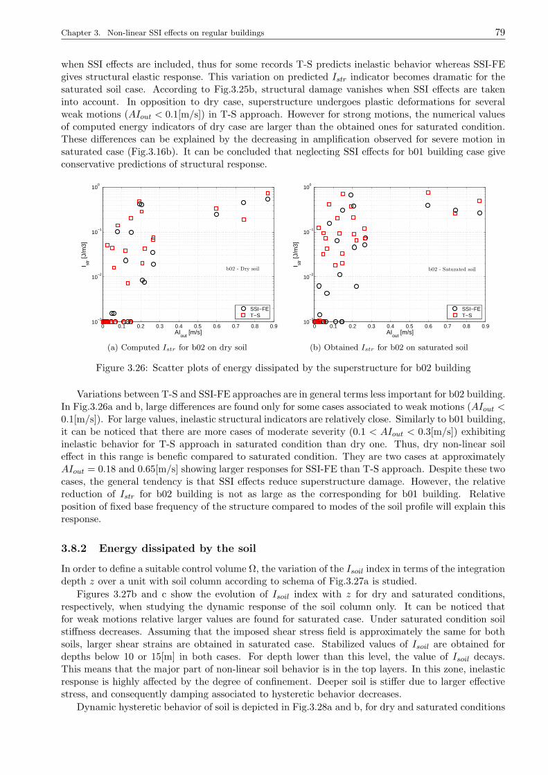
Chapter 3. Non-linear SSI effects on regular buildings 79
when SSI effects are included, thus for some records T-S predicts inelastic behavior whereas SSI-FEgives structural elastic response. This variation on predicted Istr indicator becomes dramatic for thesaturated soil case. According to Fig.3.25b, structural damage vanishes when SSI effects are takeninto account. In opposition to dry case, superstructure undergoes plastic deformations for severalweak motions (AIout < 0.1[m/s]) in T-S approach. However for strong motions, the numerical valuesof computed energy indicators of dry case are larger than the obtained ones for saturated condition.These differences can be explained by the decreasing in amplification observed for severe motion insaturated case (Fig.3.16b). It can be concluded that neglecting SSI effects for b01 building case giveconservative predictions of structural response.
0 0.1 0.2 0.3 0.4 0.5 0.6 0.7 0.8 0.910
−3
10−2
10−1
100
b02 - Dry soil
AIout
[m/s]
I str [J
/m3]
SSI−FET−S
(a) Computed Istr for b02 on dry soil
0 0.1 0.2 0.3 0.4 0.5 0.6 0.7 0.8 0.910
−3
10−2
10−1
100
b02 - Saturated soil
AIout
[m/s]
I str [J
/m3]
SSI−FET−S
(b) Obtained Istr for b02 on saturated soil
Figure 3.26: Scatter plots of energy dissipated by the superstructure for b02 building
Variations between T-S and SSI-FE approaches are in general terms less important for b02 building.In Fig.3.26a and b, large differences are found only for some cases associated to weak motions (AIout <0.1[m/s]). For large values, inelastic structural indicators are relatively close. Similarly to b01 building,it can be noticed that there are more cases of moderate severity (0.1 < AIout < 0.3[m/s]) exhibitinginelastic behavior for T-S approach in saturated condition than dry one. Thus, dry non-linear soileffect in this range is benefic compared to saturated condition. They are two cases at approximatelyAIout = 0.18 and 0.65[m/s] showing larger responses for SSI-FE than T-S approach. Despite these twocases, the general tendency is that SSI effects reduce superstructure damage. However, the relativereduction of Istr for b02 building is not as large as the corresponding for b01 building. Relativeposition of fixed base frequency of the structure compared to modes of the soil profile will explain thisresponse.
3.8.2 Energy dissipated by the soil
In order to define a suitable control volume Ω, the variation of the Isoil index in terms of the integrationdepth z over a unit with soil column according to schema of Fig.3.27a is studied.
Figures 3.27b and c show the evolution of Isoil index with z for dry and saturated conditions,respectively, when studying the dynamic response of the soil column only. It can be noticed thatfor weak motions relative larger values are found for saturated case. Under saturated condition soilstiffness decreases. Assuming that the imposed shear stress field is approximately the same for bothsoils, larger shear strains are obtained in saturated case. Stabilized values of Isoil are obtained fordepths below 10 or 15[m] in both cases. For depth lower than this level, the value of Isoil decays.This means that the major part of non-linear soil behavior is in the top layers. In this zone, inelasticresponse is highly affected by the degree of confinement. Deeper soil is stiffer due to larger effectivestress, and consequently damping associated to hysteretic behavior decreases.
Dynamic hysteretic behavior of soil is depicted in Fig.3.28a and b, for dry and saturated conditions
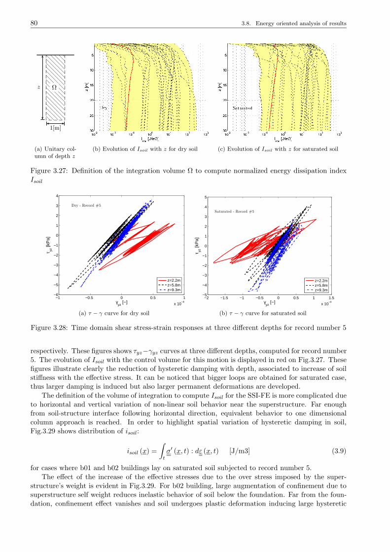
80 3.8. Energy oriented analysis of results
z Ω
1[m]
(a) Unitary col-umn of depth z
(b) Evolution of Isoil with z for dry soil (c) Evolution of Isoil with z for saturated soil
Figure 3.27: Definition of the integration volume Ω to compute normalized energy dissipation indexIsoil
−1 −0.5 0 0.5 1
x 10−4
−6
−5
−4
−3
−2
−1
0
1
2
3
4
Dry - Record #5
γyz
[−]
τ yz [k
Pa]
z=2.2mz=5.8mz=9.3m
(a) τ − γ curve for dry soil
−2 −1.5 −1 −0.5 0 0.5 1 1.5
x 10−4
−5
−4
−3
−2
−1
0
1
2
3
4
5
Saturated - Record #5
γyz
[−]
τ yz [k
Pa]
z=2.2mz=5.8mz=9.3m
(b) τ − γ curve for saturated soil
Figure 3.28: Time domain shear stress-strain responses at three different depths for record number 5
respectively. These figures shows τyz−γyz curves at three different depths, computed for record number5. The evolution of Isoil with the control volume for this motion is displayed in red on Fig.3.27. Thesefigures illustrate clearly the reduction of hysteretic damping with depth, associated to increase of soilstiffness with the effective stress. It can be noticed that bigger loops are obtained for saturated case,thus larger damping is induced but also larger permanent deformations are developed.
The definition of the volume of integration to compute Isoil for the SSI-FE is more complicated dueto horizontal and vertical variation of non-linear soil behavior near the superstructure. Far enoughfrom soil-structure interface following horizontal direction, equivalent behavior to one dimensionalcolumn approach is reached. In order to highlight spatial variation of hysteretic damping in soil,Fig.3.29 shows distribution of isoil:
isoil (x) =
∫
t
σ′ (x, t) : dε (x, t) [J/m3] (3.9)
for cases where b01 and b02 buildings lay on saturated soil subjected to record number 5.
The effect of the increase of the effective stresses due to the over stress imposed by the super-structure’s weight is evident in Fig.3.29. For b02 building, large augmentation of confinement due tosuperstructure self weight reduces inelastic behavior of soil below the foundation. Far from the foun-dation, confinement effect vanishes and soil undergoes plastic deformation inducing large hysteretic
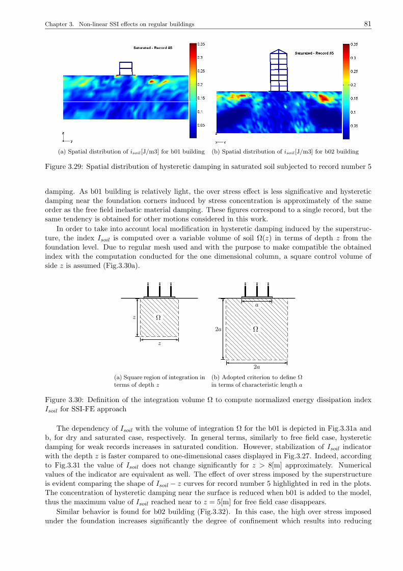
Chapter 3. Non-linear SSI effects on regular buildings 81
(a) Spatial distribution of isoil[J/m3] for b01 building (b) Spatial distribution of isoil[J/m3] for b02 building
Figure 3.29: Spatial distribution of hysteretic damping in saturated soil subjected to record number 5
damping. As b01 building is relatively light, the over stress effect is less significative and hystereticdamping near the foundation corners induced by stress concentration is approximately of the sameorder as the free field inelastic material damping. These figures correspond to a single record, but thesame tendency is obtained for other motions considered in this work.
In order to take into account local modification in hysteretic damping induced by the superstruc-ture, the index Isoil is computed over a variable volume of soil Ω(z) in terms of depth z from thefoundation level. Due to regular mesh used and with the purpose to make compatible the obtainedindex with the computation conducted for the one dimensional column, a square control volume ofside z is assumed (Fig.3.30a).
Ω
z
z
(a) Square region of integration interms of depth z
Ω
2a
2a
a
(b) Adopted criterion to define Ωin terms of characteristic length a
Figure 3.30: Definition of the integration volume Ω to compute normalized energy dissipation indexIsoil for SSI-FE approach
The dependency of Isoil with the volume of integration Ω for the b01 is depicted in Fig.3.31a andb, for dry and saturated case, respectively. In general terms, similarly to free field case, hystereticdamping for weak records increases in saturated condition. However, stabilization of Isoil indicatorwith the depth z is faster compared to one-dimensional cases displayed in Fig.3.27. Indeed, accordingto Fig.3.31 the value of Isoil does not change significantly for z > 8[m] approximately. Numericalvalues of the indicator are equivalent as well. The effect of over stress imposed by the superstructureis evident comparing the shape of Isoil − z curves for record number 5 highlighted in red in the plots.The concentration of hysteretic damping near the surface is reduced when b01 is added to the model,thus the maximum value of Isoil reached near to z = 5[m] for free field case disappears.
Similar behavior is found for b02 building (Fig.3.32). In this case, the high over stress imposedunder the foundation increases significantly the degree of confinement which results into reducing
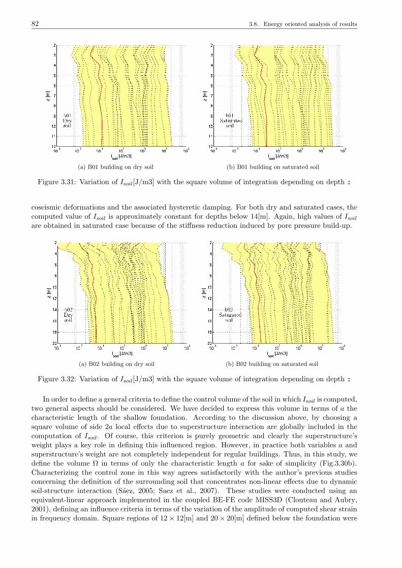
82 3.8. Energy oriented analysis of results
(a) B01 building on dry soil (b) B01 building on saturated soil
Figure 3.31: Variation of Isoil[J/m3] with the square volume of integration depending on depth z
coseismic deformations and the associated hysteretic damping. For both dry and saturated cases, thecomputed value of Isoil is approximately constant for depths below 14[m]. Again, high values of Isoilare obtained in saturated case because of the stiffness reduction induced by pore pressure build-up.
(a) B02 building on dry soil (b) B02 building on saturated soil
Figure 3.32: Variation of Isoil[J/m3] with the square volume of integration depending on depth z
In order to define a general criteria to define the control volume of the soil in which Isoil is computed,two general aspects should be considered. We have decided to express this volume in terms of a thecharacteristic length of the shallow foundation. According to the discussion above, by choosing asquare volume of side 2a local effects due to superstructure interaction are globally included in thecomputation of Isoil. Of course, this criterion is purely geometric and clearly the superstructure’sweight plays a key role in defining this influenced region. However, in practice both variables a andsuperstructure’s weight are not completely independent for regular buildings. Thus, in this study, wedefine the volume Ω in terms of only the characteristic length a for sake of simplicity (Fig.3.30b).Characterizing the control zone in this way agrees satisfactorily with the author’s previous studiesconcerning the definition of the surrounding soil that concentrates non-linear effects due to dynamicsoil-structure interaction (Saez, 2005; Saez et al., 2007). These studies were conducted using anequivalent-linear approach implemented in the coupled BE-FE code MISS3D (Clouteau and Aubry,2001), defining an influence criteria in terms of the variation of the amplitude of computed shear strainin frequency domain. Square regions of 12× 12[m] and 20× 20[m] defined below the foundation were
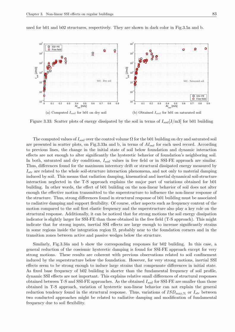
Chapter 3. Non-linear SSI effects on regular buildings 83
used for b01 and b02 structures, respectively. They are shown in dark color in Fig.3.5a and b.
0 0.1 0.2 0.3 0.4 0.5 0.6 0.7 0.8 0.910
−3
10−2
10−1
100
101
102
103
b01 - Dry soil
AIout
[m/s]
I soil [J
/m3]
SSI−FEFree field
(a) Computed Isoil for b01 on dry soil
0 0.1 0.2 0.3 0.4 0.5 0.6 0.7 0.8 0.910
−3
10−2
10−1
100
101
102
103
b01 - Saturated soil
AIout
[m/s]
I soil [J
/m3]
SSI−FEFree field
(b) Obtained Isoil for b01 on saturated soil
Figure 3.33: Scatter plots of energy dissipated by the soil in terms of Isoil[J/m3] for b01 building
The computed values of Isoil over the control volume Ω for the b01 building on dry and saturated soilare presented in scatter plots, on Fig.3.33a and b, in terms of AIout for each used record. Accordingto previous lines, the change in the initial state of soil below foundation and dynamic interactioneffects are not enough to alter significantly the hysteretic behavior of foundation’s neighboring soil.In both, saturated and dry conditions, Isoil values in free field or in SSI-FE approach are similar.Thus, differences found for the maximum interstory drift or structural dissipated energy measured byIstr are related to the whole soil-structure interaction phenomena, and not only to material dampinginduced by soil. This means that radiation damping, kinematical and inertial dynamical soil-structureinteraction neglected in the T-S approach explains the major part of variations obtained for b01building. In other words, the effect of b01 building on the non-linear behavior of soil does not alterenough the effective motion transmitted to the superstructure to influence the non-linear response ofthe structure. Thus, strong differences found in structural response of b01 building must be associatedto radiative damping and support flexibility. Of course, other aspects such as frequency content of themotion compared to the soil first elastic frequency and the superstructure also play a key role on thestructural response. Additionally, it can be noticed that for strong motions the soil energy dissipationindicator is slightly larger for SSI-FE than those obtained in the free field (T-S approach). This mightindicate that for strong inputs, inertial SSI effects are large enough to increase significantly strainsin some regions inside the integration region Ω, probably near to the foundation corners and in thetransition zones between active and passive wedges below the structure.
Similarly, Fig.3.34a and b show the corresponding responses for b02 building. In this case, ageneral reduction of the coseismic hysteretic damping is found for SSI-FE approach except for verystrong motions. These results are coherent with previous observations related to soil confinementinduced by the superstructure below the foundation. However, for very strong motions, inertial SSIeffects seem to be strong enough to induce large strains that compensate differences in initial state.As fixed base frequency of b02 building is shorter than the fundamental frequency of soil profile,dynamic SSI effects are not important. This explains relative small differences of structural responsesobtained between T-S and SSI-FE approaches. As the obtained Isoil for SSI-FE are smaller than thoseobtained in T-S approach, variation of hysteretic non-linear behavior can not explain the generalreduction tendency found in the structural response. Thus, variations of ISDmax,% or Istr betweentwo conducted approaches might be related to radiative damping and modification of fundamentalfrequency due to soil flexibility.
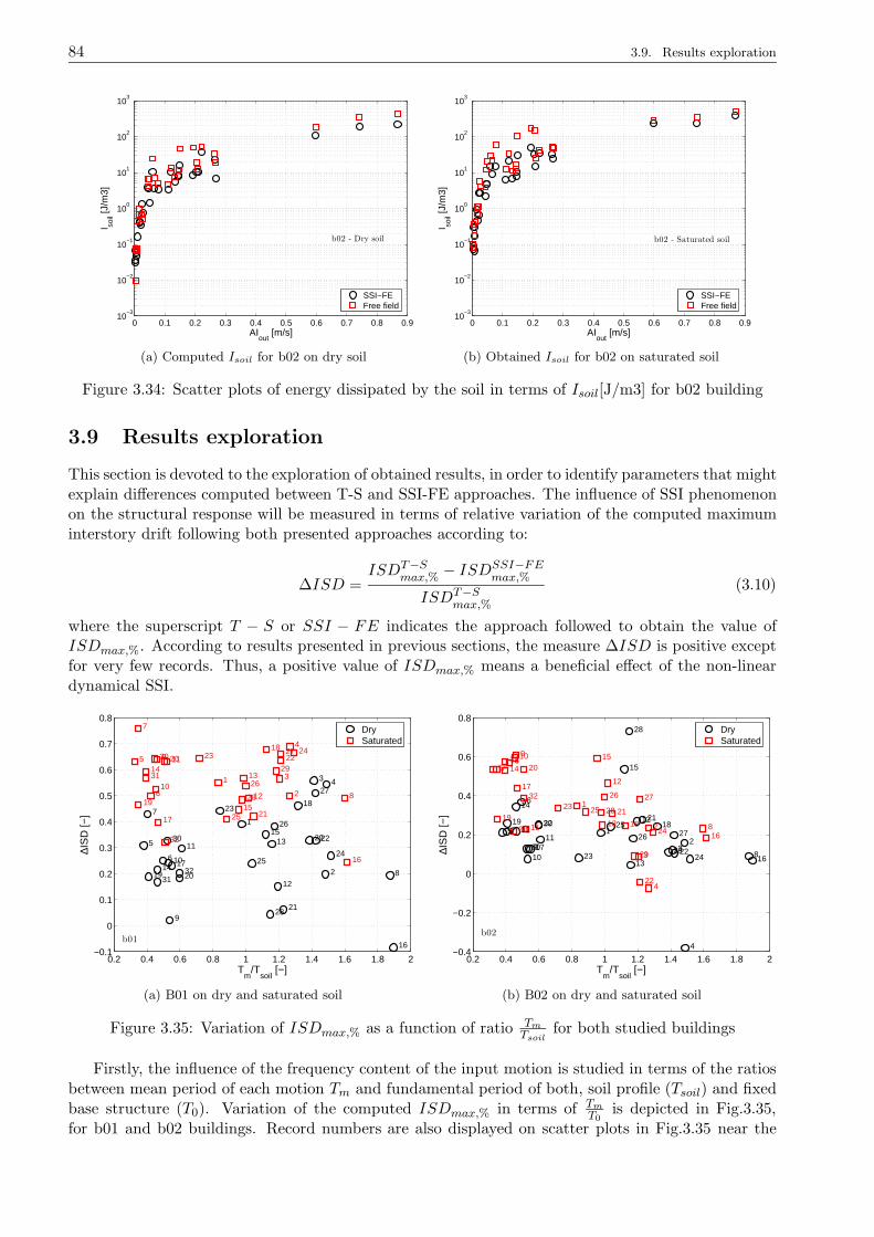
84 3.9. Results exploration
0 0.1 0.2 0.3 0.4 0.5 0.6 0.7 0.8 0.910
−3
10−2
10−1
100
101
102
103
b02 - Dry soil
AIout
[m/s]
I soil [J
/m3]
SSI−FEFree field
(a) Computed Isoil for b02 on dry soil
0 0.1 0.2 0.3 0.4 0.5 0.6 0.7 0.8 0.910
−3
10−2
10−1
100
101
102
103
b02 - Saturated soil
AIout
[m/s]
I soil [J
/m3]
SSI−FEFree field
(b) Obtained Isoil for b02 on saturated soil
Figure 3.34: Scatter plots of energy dissipated by the soil in terms of Isoil[J/m3] for b02 building
3.9 Results exploration
This section is devoted to the exploration of obtained results, in order to identify parameters that mightexplain differences computed between T-S and SSI-FE approaches. The influence of SSI phenomenonon the structural response will be measured in terms of relative variation of the computed maximuminterstory drift following both presented approaches according to:
∆ISD =ISDT−S
max,% − ISDSSI−FEmax,%
ISDT−Smax,%
(3.10)
where the superscript T − S or SSI − FE indicates the approach followed to obtain the value ofISDmax,%. According to results presented in previous sections, the measure ∆ISD is positive exceptfor very few records. Thus, a positive value of ISDmax,% means a beneficial effect of the non-lineardynamical SSI.
0.2 0.4 0.6 0.8 1 1.2 1.4 1.6 1.8 2−0.1
0
0.1
0.2
0.3
0.4
0.5
0.6
0.7
0.8
1
2
3 4
5
6
7
8
9
10
11
12
13
14
15
16
17
18
19 20
21
22
23
2425
26
27
28
2930
3132
1
2
3
4
5
6
7
8
9
10
11
12
1314
15
16
17
18
19
20
21
222324
25
26
27
28
29
30
31
32
b01
Tm
/Tsoil
[−]
∆IS
D [−
]
DrySaturated
(a) B01 on dry and saturated soil
0.2 0.4 0.6 0.8 1 1.2 1.4 1.6 1.8 2−0.4
−0.2
0
0.2
0.4
0.6
0.8
12
3
4
5
6
7
8910
11
12
13
14
15
1617
1819 2021
2223 24
25
26 27
28
2930
3132
1
2
3
4
56
7
8
910
11
12
13
14
15
16
17
1819
20
21
22
23
24
25
26 27
28
29
30
31
32
b02
Tm
/Tsoil
[−]
∆IS
D [−
]
DrySaturated
(b) B02 on dry and saturated soil
Figure 3.35: Variation of ISDmax,% as a function of ratio Tm
Tsoilfor both studied buildings
Firstly, the influence of the frequency content of the input motion is studied in terms of the ratiosbetween mean period of each motion Tm and fundamental period of both, soil profile (Tsoil) and fixedbase structure (T0). Variation of the computed ISDmax,% in terms of Tm
T0is depicted in Fig.3.35,
for b01 and b02 buildings. Record numbers are also displayed on scatter plots in Fig.3.35 near the
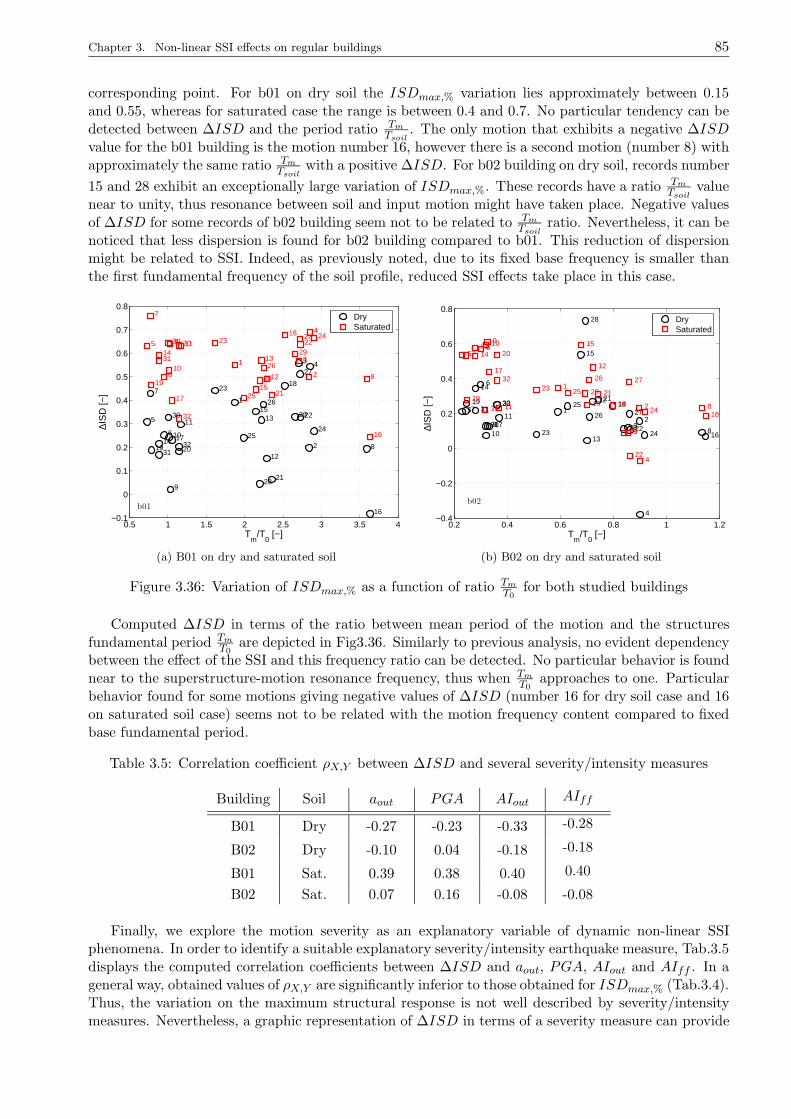
Chapter 3. Non-linear SSI effects on regular buildings 85
corresponding point. For b01 on dry soil the ISDmax,% variation lies approximately between 0.15and 0.55, whereas for saturated case the range is between 0.4 and 0.7. No particular tendency can bedetected between ∆ISD and the period ratio Tm
Tsoil. The only motion that exhibits a negative ∆ISD
value for the b01 building is the motion number 16, however there is a second motion (number 8) withapproximately the same ratio Tm
Tsoilwith a positive ∆ISD. For b02 building on dry soil, records number
15 and 28 exhibit an exceptionally large variation of ISDmax,%. These records have a ratio Tm
Tsoilvalue
near to unity, thus resonance between soil and input motion might have taken place. Negative valuesof ∆ISD for some records of b02 building seem not to be related to Tm
Tsoilratio. Nevertheless, it can be
noticed that less dispersion is found for b02 building compared to b01. This reduction of dispersionmight be related to SSI. Indeed, as previously noted, due to its fixed base frequency is smaller thanthe first fundamental frequency of the soil profile, reduced SSI effects take place in this case.
0.5 1 1.5 2 2.5 3 3.5 4−0.1
0
0.1
0.2
0.3
0.4
0.5
0.6
0.7
0.8
1
2
3 4
5
6
7
8
9
10
11
12
13
14
15
16
17
18
19 20
21
22
23
2425
26
27
28
2930
3132
1
2
3
4
5
6
7
8
9
10
11
12
1314
15
16
17
18
19
20
21
222324
25
26
27
28
29
30
31
32
b01
Tm
/T0 [−]
∆IS
D [−
]
DrySaturated
(a) B01 on dry and saturated soil
0.2 0.4 0.6 0.8 1 1.2−0.4
−0.2
0
0.2
0.4
0.6
0.8
12
3
4
5
6
7
8910
11
12
13
14
15
1617
1819 2021
2223 24
25
26 27
28
2930
3132
1
2
3
4
56
7
8
910
11
12
13
14
15
16
17
1819
20
21
22
23
24
25
26 27
28
29
30
31
32
b02
Tm
/T0 [−]
∆IS
D [−
]
DrySaturated
(b) B02 on dry and saturated soil
Figure 3.36: Variation of ISDmax,% as a function of ratio Tm
T0for both studied buildings
Computed ∆ISD in terms of the ratio between mean period of the motion and the structuresfundamental period Tm
T0are depicted in Fig3.36. Similarly to previous analysis, no evident dependency
between the effect of the SSI and this frequency ratio can be detected. No particular behavior is foundnear to the superstructure-motion resonance frequency, thus when Tm
T0approaches to one. Particular
behavior found for some motions giving negative values of ∆ISD (number 16 for dry soil case and 16on saturated soil case) seems not to be related with the motion frequency content compared to fixedbase fundamental period.
Table 3.5: Correlation coefficient ρX,Y between ∆ISD and several severity/intensity measures
Building Soil aout PGA AIout AIff
B01 Dry -0.27 -0.23 -0.33 -0.28
B02 Dry -0.10 0.04 -0.18 -0.18
B01 Sat. 0.39 0.38 0.40 0.40
B02 Sat. 0.07 0.16 -0.08 -0.08
Finally, we explore the motion severity as an explanatory variable of dynamic non-linear SSIphenomena. In order to identify a suitable explanatory severity/intensity earthquake measure, Tab.3.5displays the computed correlation coefficients between ∆ISD and aout, PGA, AIout and AIff . In ageneral way, obtained values of ρX,Y are significantly inferior to those obtained for ISDmax,% (Tab.3.4).Thus, the variation on the maximum structural response is not well described by severity/intensitymeasures. Nevertheless, a graphic representation of ∆ISD in terms of a severity measure can provide
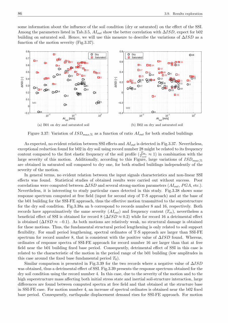
86 3.9. Results exploration
some information about the influence of the soil condition (dry or saturated) on the effect of the SSI.Among the parameters listed in Tab.3.5, AIout show the better correlation with ∆ISD, expect for b02building on saturated soil. Hence, we will use this measure to describe the variations of ∆ISD as afunction of the motion severity (Fig.3.37).
10−2
10−1
100
−0.1
0
0.1
0.2
0.3
0.4
0.5
0.6
0.7
0.8
1
2
34
5
6
7
8
9
10
11
12
13
14
15
16
17
18
1920
21
22
23
2425
26
27
28
29 30
3132
1
2
3
4
5
6
7
8
9
10
11
12
1314
15
16
17
18
19
20
21
222324
25
26
27
28
29
30
31
32
b01
AIout
[m/s]
∆IS
D [−
]
DrySaturated
(a) B01 on dry and saturated soil
10−2
10−1
100
−0.4
−0.2
0
0.2
0.4
0.6
0.8
12
3
4
5
6
7
89
10
11
12
13
14
15
1617
18 192021
222324
25
2627
28
29 30
3132
1
2
3
4
56
7
8
9 10
11
12
13
14
15
16
17
1819
20
21
22
23
24
25
2627
28
29
30
31
32
b02
AIout
[m/s]∆I
SD
[−]
DrySaturated
(b) B02 on dry and saturated soil
Figure 3.37: Variation of ISDmax,% as a function of ratio AIout for both studied buildings
As expected, no evident relation between SSI effects and AIout is detected in Fig.3.37. Nevertheless,exceptional reduction found for b02 in dry soil using record number 28 might be related to its frequencycontent compared to the first elastic frequency of the soil profile ( Tm
Tsoil≈ 1) in combination with the
large severity of this motion. Additionally, according to this Figure, large variations of ISDmax,%
are obtained in saturated soil compared to dry one, for both studied buildings independently of theseverity of the motion.
In general terms, no evident relation between the input signals characteristics and non-linear SSIeffects was found. Statistical studies of obtained results were carried out without success. Poorcorrelations were computed between ∆ISD and several strong-motion parameters (AIout, PGA, etc.).Nevertheless, it is interesting to study particular cases detected in this study. Fig.3.38 shows someresponse spectrum computed at free field (input for second step of T-S approach) and at the base ofthe b01 building for the SSI-FE approach, thus the effective motion transmitted to the superstructurefor the dry soil condition. Fig.3.38a an b correspond to records number 8 and 16, respectively. Bothrecords have approximatively the same severity (AIout) and frequency content (Tm), nevertheless abeneficial effect of SSI is obtained for record 8 (∆ISD ≈ 0.2) while for record 16 a detrimental effectis obtained (∆ISD ≈ −0.1). As both motions are relatively weak, no structural damage is obtainedfor these motions. Thus, the fundamental structural period lengthening is only related to soil supportflexibility. For small period lengthening, spectral ordinates of T-S approach are larger than SSI-FEspectrum for record number 8, that is consistent with the positive value of ∆ISD found. Whereas,ordinates of response spectra of SSI-FE approach for record number 16 are larger than that at freefield near the b01 building fixed base period. Consequently, detrimental effect of SSI in this case isrelated to the characteristic of the motion in the period range of the b01 building (low amplitudes inthis case around the fixed base fundamental period T0).
Similar comparison is presented in Fig.3.39 for the two records where a negative value of ∆ISDwas obtained, thus a detrimental effect of SSI. Fig.3.39 presents the response spectrum obtained for thedry soil condition using the record number 4. In this case, due to the severity of the motion and to thehigh superstructure mass affecting both initial stress state and inertial soil-structure interaction, largedifferences are found between computed spectra at free field and that obtained at the structure basein SSI-FE case. For motion number 4, an increase of spectral ordinates is obtained near the b02 fixedbase period. Consequently, earthquake displacement demand rises for SSI-FE approach. For motion
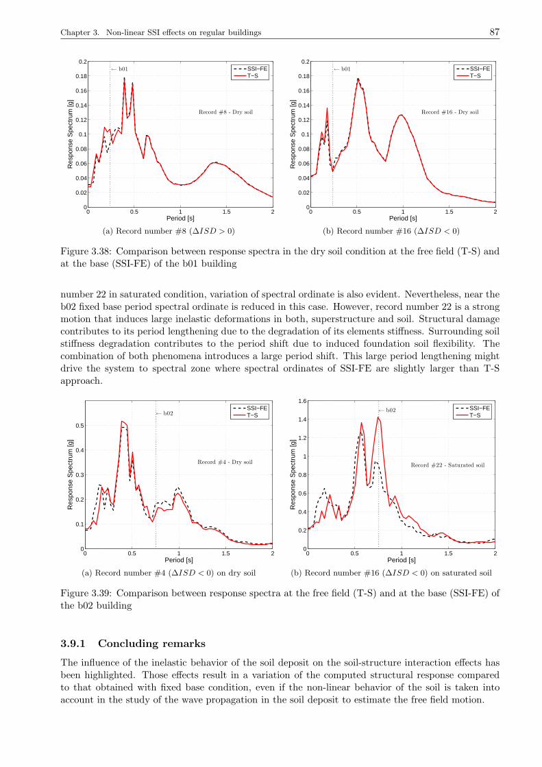
Chapter 3. Non-linear SSI effects on regular buildings 87
0 0.5 1 1.5 20
0.02
0.04
0.06
0.08
0.1
0.12
0.14
0.16
0.18
0.2← b01
Record #8 - Dry soil
Period [s]
Res
pons
e S
pect
rum
[g]
SSI−FET−S
(a) Record number #8 (∆ISD > 0)
0 0.5 1 1.5 20
0.02
0.04
0.06
0.08
0.1
0.12
0.14
0.16
0.18
0.2← b01
Record #16 - Dry soil
Period [s]
Res
pons
e S
pect
rum
[g]
SSI−FET−S
(b) Record number #16 (∆ISD < 0)
Figure 3.38: Comparison between response spectra in the dry soil condition at the free field (T-S) andat the base (SSI-FE) of the b01 building
number 22 in saturated condition, variation of spectral ordinate is also evident. Nevertheless, near theb02 fixed base period spectral ordinate is reduced in this case. However, record number 22 is a strongmotion that induces large inelastic deformations in both, superstructure and soil. Structural damagecontributes to its period lengthening due to the degradation of its elements stiffness. Surrounding soilstiffness degradation contributes to the period shift due to induced foundation soil flexibility. Thecombination of both phenomena introduces a large period shift. This large period lengthening mightdrive the system to spectral zone where spectral ordinates of SSI-FE are slightly larger than T-Sapproach.
0 0.5 1 1.5 20
0.1
0.2
0.3
0.4
0.5
← b02
Record #4 - Dry soil
Period [s]
Res
pons
e S
pect
rum
[g]
SSI−FET−S
(a) Record number #4 (∆ISD < 0) on dry soil
0 0.5 1 1.5 20
0.2
0.4
0.6
0.8
1
1.2
1.4
1.6
← b02
Record #22 - Saturated soil
Period [s]
Res
pons
e S
pect
rum
[g]
SSI−FET−S
(b) Record number #16 (∆ISD < 0) on saturated soil
Figure 3.39: Comparison between response spectra at the free field (T-S) and at the base (SSI-FE) ofthe b02 building
3.9.1 Concluding remarks
The influence of the inelastic behavior of the soil deposit on the soil-structure interaction effects hasbeen highlighted. Those effects result in a variation of the computed structural response comparedto that obtained with fixed base condition, even if the non-linear behavior of the soil is taken intoaccount in the study of the wave propagation in the soil deposit to estimate the free field motion.

88 3.10. Liquefiable soil
Evaluation of the dissipated energies has shown that the initial state modification induced by theself weight of the superstructure contributes to increase the stiffness of the soil below the foundation.This additional confinement reduces hysteretic behavior under dynamic loading, compensating strainfield generated by the superstructure’s oscillations. However, for strong motions, this compensationseems to be surpassed by SSI inertial effects for low-rise buildings.
Generalization of SSI effects on displacement demand for a given building on a defined soil wasunsuccessful. Large dispersion of results can be associated to the complexity of natural earthquakes,where spectral-amplitude characteristics can modify significantly the global response of the superstruc-ture. This phenomenon was highlighted comparing response spectra of records showing detrimentalSSI effects.
The next section is devoted to apply the presented modified plane-strain approach to the particularcase of liquefiable soil. With this purpose, both studied buildings are analyzed on a locally liquefiableprofile following the same approaches presented before and using the same record database.
3.10 Liquefiable soil
This section is devoted to evaluate the influence of soil non-linearity on the soil-foundation-structureinteraction phenomena for a liquefiable soil. The purpose of this presentation is to better understandthe effect of the liquefaction on the superstructure’s response, as well as to investigate the modificationintroduced in the liquefaction phenomena due to the presence of the superstructure.
This study is an extension of the investigation of Lopez-Caballero and Modaressi-FarahmandRazavi (2008) conducted for three linear-elastic SDOFs on a liquefiable profile. In present study,we introduce non-linear behavior for the superstructure and we apply the modified plane-strain con-dition described previously. The fist study was conducted for four European earthquakes of verydifferent frequency contents scaled to several outcropping amplitudes. In the present study we takeadvantage of the Design of Experiments methodology to select a motion database as is described in§3.5. Thus, the analysis is conducted for b01 and b02 non-linear buildings described in appendix I forthe 32 records listed in appendix J.
The studied site is composed principally of clay layers overlaid by 22[m] of loose sand, i.e. relativedensity of Dr < 50%. Site measurement of SPTN60 and low-strain shear wave velocities are givenin Fig.3.40. According to SPTN60 profile, liquefaction phenomenon might take places between 4and 15[m], where SPTN60 value is lower than 10. Soil deeper than 22[m] is constituted mainly ofoverconsolidated clay. Non-linear behavior is expected only for the first 29[m], thus isotropic linearelastic behavior is assumed for soil deeper than 29[m]. The deformable bedrock is placed at 40[m]depth.
0 20 40 60
0
5
10
15
20
25
30
35
40
45
SPT − N60
Dep
th [m
]
0 200 400 600
0
5
10
15
20
25
30
35
40
45
Vs [m/s]
Dep
th [m
]
Figure 3.40: SPT and low-strain shear velocity profile of the studied site (after Lopez-Caballero andModaressi-Farahmand Razavi (2008))

Chapter 3. Non-linear SSI effects on regular buildings 89
The ECP’s elastoplastic cyclic multi-mechanism model Aubry et al. (1982); Hujeux (1985) is usedto represent the soil behavior. Theoretical formulation and physical interpretations of different pa-rameters was extensively treated in Appendix E. The soil model’s parameters are obtained usingthe methodology suggested by Lopez-Caballero et al. (2003); Lopez-Caballero et al. (2007) describedbriefly in §1.3.4. In order to verify the model’s parameters and to characterize the liquefaction resis-tance of sand placed between 3.5 and 9[m] depth, the behavior is studied by simulating drained cyclicshear (DCS) tests and undrained stress controlled cyclic shear test. Parameter sets and comparisonof simulations with references curves are provided in appendix H.2.
3.10.1 Ground response
According to approaches described in §3.3, first part of T-S strategy consists in obtaining the free fieldresponse associated to record database selected for the analysis. Fig.3.41a presents the variation ofpeak ground acceleration PGA at free field as function of the imposed peak acceleration at outcroppingbedrock aout. It can be noticed that amplification of the peak acceleration takes places for aout < 0.1[g].Maximum amplification reached for this range of aout is approximately up to 2.5 times the amplitude ofthe imposed motion. For amplitudes larger than 0.1[g], the apparition of the liquefaction phenomenonattenuates strongly seismic motion resulting in a relative de-amplification of acceleration peaks.
0 0.05 0.1 0.15 0.2 0.25 0.3 0.350
0.05
0.1
0.15
0.2
0.25
1:1
1:2.5
12
3
45
6
7
8
9
10
11
12
13
14
15
16
17
18
19
20
21
22
23
24
25
2627
28
29
30
31
32
aout
[g]
PG
A [g
]
Liquefiable soil
(a) Computed PGA for liquefiable soil (b) Obtained pore pressure excess in the soil profile fordifferent used records
Figure 3.41: Effect of excess pore pressure on free field response
In order to define depth and thickness of zones where liquefaction might take place, Fig.3.41b showsthe envelope of induced pore pressure excess ∆uw profile at the end of the analyses (tend). Profilesassociated to each motion are displayed in dotted lines. It can be concluded, that depending on theinput, liquefaction take places between 2 and 10[m] approximately. However, only strong motions areable to induce liquefaction. In order to study the influence of the frequency content and the severityof the motion on triggering liquefaction, we define the mean liquefaction index Q(t) at a time t as:
Q(t) =1
Ω
∫
ΩRu (x, t) dV =
1
Ω
∫
Ω
∆uw (x, t)
σ′zz (x, 0)dV (3.11)
where Ru(x, t) is the pore pressure ratio at a material point x at a time t, computed from the porepressure excess ∆uw(x, t) and the initial vertical effective stress σ′zz(x, 0) at the same material point.The control volume Ω is defined as presented in Fig.3.27a in terms of the depth z. According to porepressure built-up profile on Fig.3.41b, we select a volume of integration between z = 2 and z = 10[m],where liquefaction phenomenon is expected. Fig.3.42a and b show computed liquefaction index forthe 32 used records in terms of aout and AI respectively. It can be noticed that a better correlation

90 3.10. Liquefiable soil
is found for Arias’s intensity than for outcrop acceleration amplitude, thus triggering of liquefactioncan be better explained by a measure of energy than by a simple amplitude parameter. In this case,for AIout larger than 0.2[m/s] a liquefied zone is found (motions number 1, 2, 10, 11, 15, 21, 22, 28and 29 highlighted in red dashed lines on Fig.3.41b). The computed Q(tend) for these records is largerthan 0.3 and the computed PGA is smaller or equal to aout.
0 0.05 0.1 0.15 0.2 0.25 0.3 0.350
0.1
0.2
0.3
0.4
0.5
0.6
0.7
0.8
0.9
1
2
3
45
6
78
9
10
11
12
13
14
15
16 1718
1920
21
22
23
24 25
2627
28
29
3031
32
aout
[g]
Q(t
end)
[−]
2<z<10m
(a) Q(tend) in terms of acceleration amplitude at out-crop
0 0.1 0.2 0.3 0.4 0.5 0.6 0.7 0.8 0.90
0.1
0.2
0.3
0.4
0.5
0.6
0.7
0.8
0.9
1
2
3
45
6
78
9
10
11
12
13
14
15
161718
1920
21
22
23
2425
2627
28
29
3031
32
AIout
[m/s]Q
(ten
d) [−
]
2<z<10m
(b) Computed Q(tend) as a function of Arias’intensityat outcrop
Figure 3.42: Obtained mean liquefaction index at tend in soil profile for different records
Several authors (Koutsourelakis et al., 2002; Popescu, 2002) have suggested that for motions ableto induce liquefaction, the liquefaction zone depends on the frequency content of the motion. Tab.3.6shows soil depths where liquefaction takes places (Ru(tend) = 1) and the ratio Tm
Tsoilbetween mean
period of the input and the first elastic mode of the soil profile Tsoil. As frequency contents andamplitude change between records, it is difficult to obtain general tendencies. However, these resultsindicate that liquefaction occurs between 2− 3[m] for records with Tm < Tsoil. When Tm value is nearto Tsoil, a deeper liquefaction zone appears (around 6[m]) in general terms. If Tm
Tsoils> 1, a liquefaction
zone is placed near to 5[m]. Theses tendencies agree with the results provided by Lopez-Caballero andModaressi-Farahmand Razavi (2008) for the same soil profile using scaled natural motions.
Table 3.6: Region of soil where liquefaction is induced
Record DepthTm
Tsoil
1 3− 5 0.792 3− 8 1.076 2− 3 0.4010 5− 6 0.4211 2− 3 0.4615 2− 3 and 6− 7 0.8821 2− 5 and 7− 9 0.9522 3− 5 1.0728 3− 6 0.9529 5− 6 1.05
Very strong motions inducing large liquefaction zones (record number 2, 21 and 28) were recordedin geological conditions corresponding to stiff soil classification according to information available inAmbraseys et al. (2004). This category is associated to a Vs,30 value larger than 400[m/s]. As concernsthese three motions, the range is between 400 − 450 [m/s], thus we cannot discard some site effects
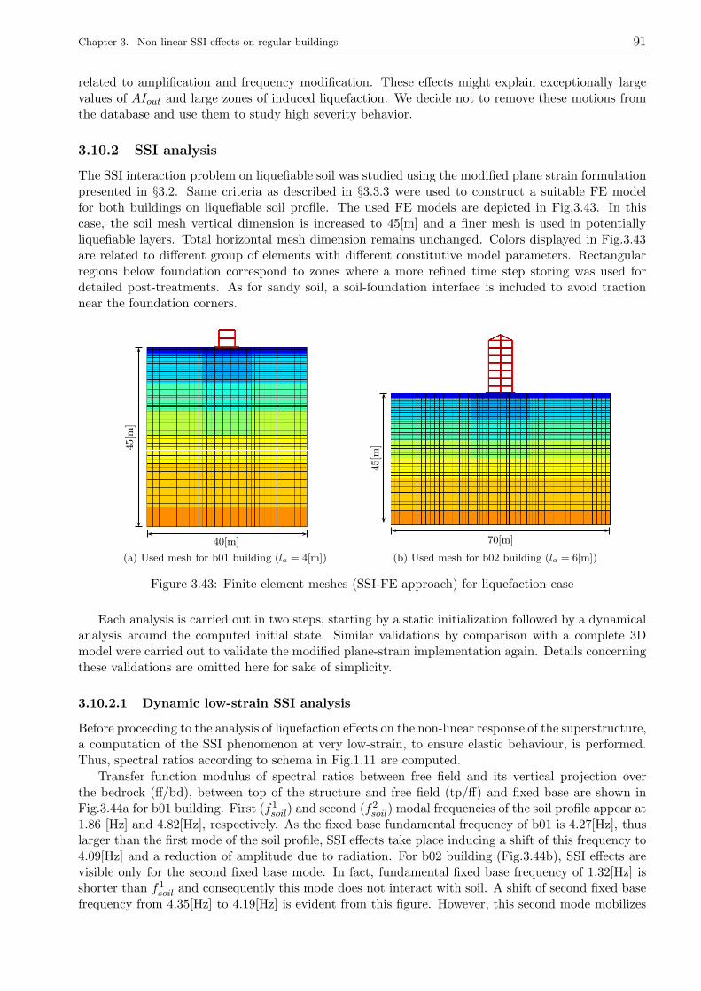
Chapter 3. Non-linear SSI effects on regular buildings 91
related to amplification and frequency modification. These effects might explain exceptionally largevalues of AIout and large zones of induced liquefaction. We decide not to remove these motions fromthe database and use them to study high severity behavior.
3.10.2 SSI analysis
The SSI interaction problem on liquefiable soil was studied using the modified plane strain formulationpresented in §3.2. Same criteria as described in §3.3.3 were used to construct a suitable FE modelfor both buildings on liquefiable soil profile. The used FE models are depicted in Fig.3.43. In thiscase, the soil mesh vertical dimension is increased to 45[m] and a finer mesh is used in potentiallyliquefiable layers. Total horizontal mesh dimension remains unchanged. Colors displayed in Fig.3.43are related to different group of elements with different constitutive model parameters. Rectangularregions below foundation correspond to zones where a more refined time step storing was used fordetailed post-treatments. As for sandy soil, a soil-foundation interface is included to avoid tractionnear the foundation corners.
40[m]
45[m
]
(a) Used mesh for b01 building (la = 4[m])
70[m]
45[m
]
(b) Used mesh for b02 building (la = 6[m])
Figure 3.43: Finite element meshes (SSI-FE approach) for liquefaction case
Each analysis is carried out in two steps, starting by a static initialization followed by a dynamicalanalysis around the computed initial state. Similar validations by comparison with a complete 3Dmodel were carried out to validate the modified plane-strain implementation again. Details concerningthese validations are omitted here for sake of simplicity.
3.10.2.1 Dynamic low-strain SSI analysis
Before proceeding to the analysis of liquefaction effects on the non-linear response of the superstructure,a computation of the SSI phenomenon at very low-strain, to ensure elastic behaviour, is performed.Thus, spectral ratios according to schema in Fig.1.11 are computed.
Transfer function modulus of spectral ratios between free field and its vertical projection overthe bedrock (ff/bd), between top of the structure and free field (tp/ff) and fixed base are shown inFig.3.44a for b01 building. First (f1
soil) and second (f2soil) modal frequencies of the soil profile appear at
1.86 [Hz] and 4.82[Hz], respectively. As the fixed base fundamental frequency of b01 is 4.27[Hz], thuslarger than the first mode of the soil profile, SSI effects take place inducing a shift of this frequency to4.09[Hz] and a reduction of amplitude due to radiation. For b02 building (Fig.3.44b), SSI effects arevisible only for the second fixed base mode. In fact, fundamental fixed base frequency of 1.32[Hz] isshorter than f1
soil and consequently this mode does not interact with soil. A shift of second fixed basefrequency from 4.35[Hz] to 4.19[Hz] is evident from this figure. However, this second mode mobilizes
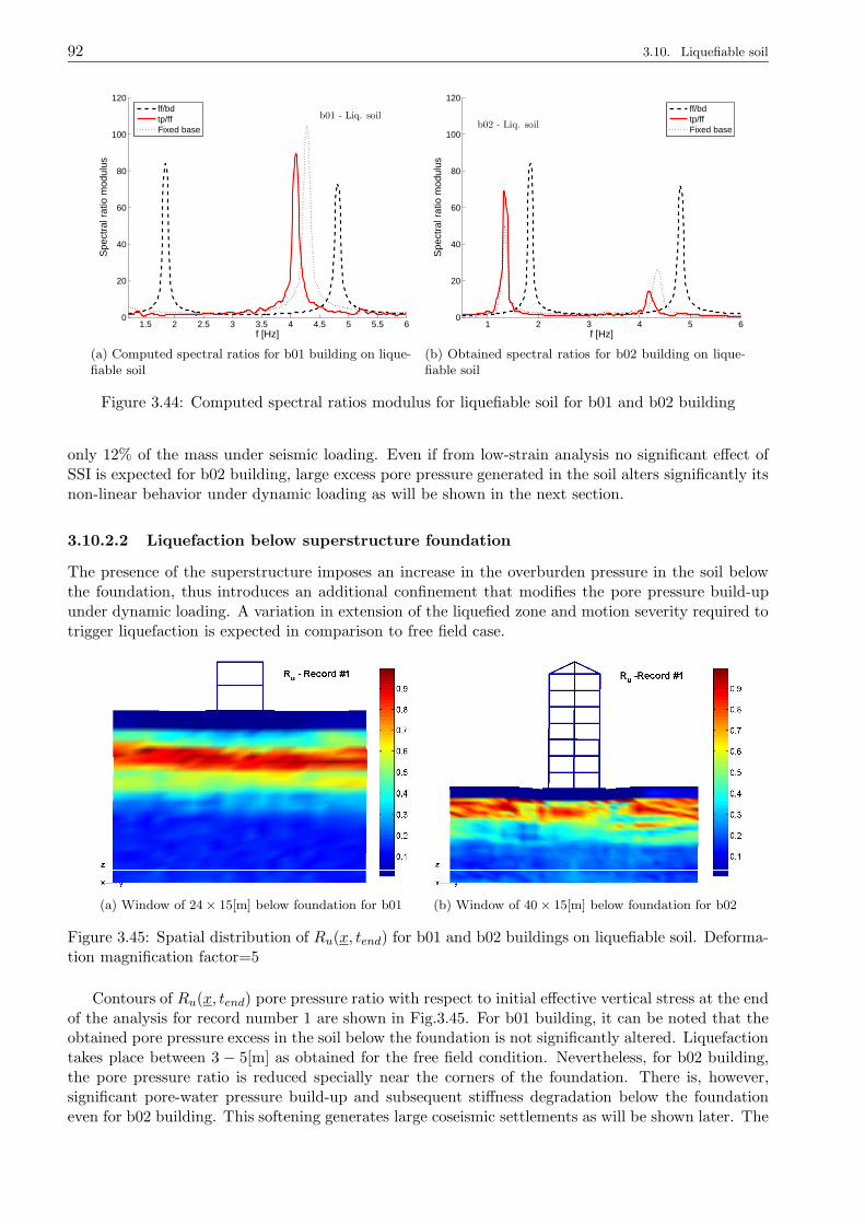
92 3.10. Liquefiable soil
1.5 2 2.5 3 3.5 4 4.5 5 5.5 60
20
40
60
80
100
120
b01 - Liq. soil
f [Hz]
Spe
ctra
l rat
io m
odul
usff/bdtp/ffFixed base
(a) Computed spectral ratios for b01 building on lique-fiable soil
1 2 3 4 5 60
20
40
60
80
100
120
b02 - Liq. soil
f [Hz]
Spe
ctra
l rat
io m
odul
us
ff/bdtp/ffFixed base
(b) Obtained spectral ratios for b02 building on lique-fiable soil
Figure 3.44: Computed spectral ratios modulus for liquefiable soil for b01 and b02 building
only 12% of the mass under seismic loading. Even if from low-strain analysis no significant effect ofSSI is expected for b02 building, large excess pore pressure generated in the soil alters significantly itsnon-linear behavior under dynamic loading as will be shown in the next section.
3.10.2.2 Liquefaction below superstructure foundation
The presence of the superstructure imposes an increase in the overburden pressure in the soil belowthe foundation, thus introduces an additional confinement that modifies the pore pressure build-upunder dynamic loading. A variation in extension of the liquefied zone and motion severity required totrigger liquefaction is expected in comparison to free field case.
(a) Window of 24 × 15[m] below foundation for b01 (b) Window of 40 × 15[m] below foundation for b02
Figure 3.45: Spatial distribution of Ru(x, tend) for b01 and b02 buildings on liquefiable soil. Deforma-tion magnification factor=5
Contours of Ru(x, tend) pore pressure ratio with respect to initial effective vertical stress at the endof the analysis for record number 1 are shown in Fig.3.45. For b01 building, it can be noted that theobtained pore pressure excess in the soil below the foundation is not significantly altered. Liquefactiontakes place between 3 − 5[m] as obtained for the free field condition. Nevertheless, for b02 building,the pore pressure ratio is reduced specially near the corners of the foundation. There is, however,significant pore-water pressure build-up and subsequent stiffness degradation below the foundationeven for b02 building. This softening generates large coseismic settlements as will be shown later. The
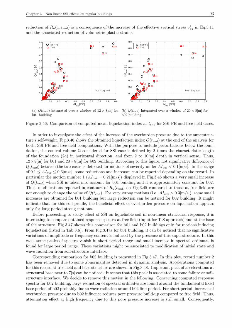
Chapter 3. Non-linear SSI effects on regular buildings 93
reduction of Ru(x, tend) is a consequence of the increase of the effective vertical stress σ′zz in Eq.3.11and the associated reduction of volumetric plastic strains.
0 0.1 0.2 0.3 0.4 0.5 0.6 0.7 0.8 0.90
0.1
0.2
0.3
0.4
0.5
0.6
0.7
0.8
0.9
1
2
3
45
6
78
9
10
11
12
13
14
15
161718
1920
21
22
23
2425
2627
28
29
3031
32
b01 - Liq. soil
AIout
[m/s]
Q(t
end)
[−]
SSI−FET−S
(a) Q(tend) integrated over a window of 12 × 8[m] forb01 building
0 0.1 0.2 0.3 0.4 0.5 0.6 0.7 0.8 0.90
0.1
0.2
0.3
0.4
0.5
0.6
0.7
0.8
0.9
1
2
3
45
6
78
9
10
11
12
13
14
15
161718
1920
21
22
23
2425
2627
28
29
3031
32
b02 - Liq. soil
AIout
[m/s]
Q(t
end)
[−]
SSI−FET−S
(b) Q(tend) integrated over a window of 20 × 8[m] forb02 building
Figure 3.46: Comparison of computed mean liquefaction index at tend for SSI-FE and free field cases.
In order to investigate the effect of the increase of the overburden pressure due to the superstruc-ture’s self-weight, Fig.3.46 shows the obtained liquefaction index Q(tend) at the end of the analysis forboth, SSI-FE and free field compuations. With the purpose to include perturbations below the foun-dation, the control volume Ω considered for SSI case is defined by 2 times the characteristic lengthof the foundation (2a) in horizontal direction, and from 2 to 10[m] depth in vertical sense. Thus,12×8[m] for b01 and 20×8[m] for b02 building. According to this figure, not significative difference ofQ(tend) between the two cases is detected for motions of severity under AIout < 0.1[m/s]. In the rangeof 0.1 ≤ AIout ≤ 0.3[m/s], some reductions and increases can be reported depending on the record. Inparticular the motion number 1 (AIout = 0.21[m/s]) displayed in Fig.3.46 shows a very small increaseof Q(tend) when SSI is taken into account for b01 building and it is approximately constant for b02.Thus, modifications reported in contours of Ru(tend) on Fig.3.45 compared to those at free field arenot enough to change the value of Q(tend). For very strong motions (i.e. AIout > 0.3[m/s]), some smallincreases are obtained for b01 building but large reduction can be noticed for b02 building. It mightindicate that for this soil profile, the beneficial effect of overburden pressure on liquefaction appearsonly for long period strong motions.
Before proceeding to study effect of SSI on liquefiable soil in non-linear structural response, it isinteresting to compare obtained response spectra at free field (input for T-S approach) and at the baseof the structure. Fig.3.47 shows this comparison for b01 and b02 buildings only for motions inducingliquefaction (listed in Tab.3.6). From Fig.3.47a for b01 building, it can be noticed that no significativevariations of amplitude or frequency content is induced by the presence of this superstructure. In thiscase, some peaks of spectra vanish in short period range and small increase in spectral ordinates isfound for large period range. These variations might be associated to modification of initial state andwave radiation from soil-structure interface.
Corresponding comparison for b02 building is presented in Fig.3.47. In this plot, record number 2has been removed due to some abnormalities detected in dynamic analysis. Accelerations computedfor this record at free field and base structure are shown in Fig.3.48. Important peak of accelerations atstructural base near to 7[s] can be noticed. It seems that this peak is associated to some failure at soil-structure interface. We decide to remove this motion in the following. Concerning computed responsespectra for b02 building, large reduction of spectral ordinates are found around the fundamental fixedbase period of b02 probably due to wave radiation around b02 first period. For short period, increase ofoverburden pressure due to b02 influence reduces pore pressure build-up compared to free field. Thus,attenuation effect at high frequency due to this pore pressure increase is still small. Consequently,
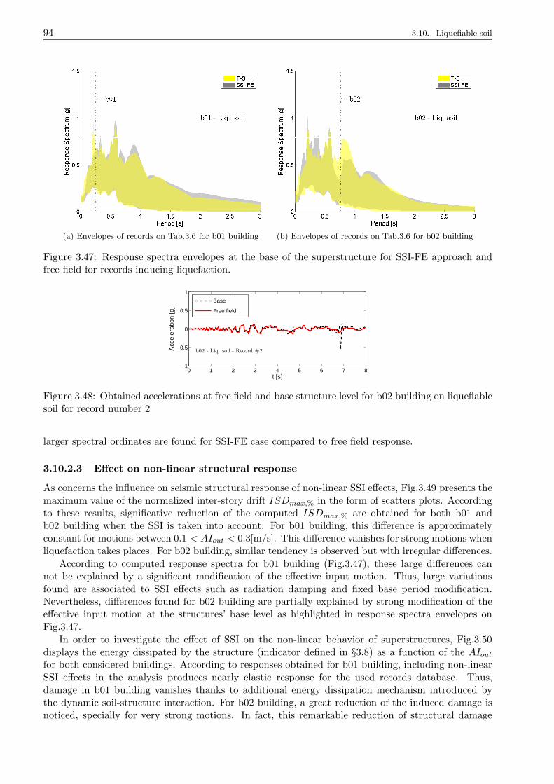
94 3.10. Liquefiable soil
(a) Envelopes of records on Tab.3.6 for b01 building (b) Envelopes of records on Tab.3.6 for b02 building
Figure 3.47: Response spectra envelopes at the base of the superstructure for SSI-FE approach andfree field for records inducing liquefaction.
0 1 2 3 4 5 6 7 8−1
−0.5
0
0.5
1
b02 - Liq. soil - Record #2
t [s]
Acc
eler
atio
n [g
]
Base
Free field
Figure 3.48: Obtained accelerations at free field and base structure level for b02 building on liquefiablesoil for record number 2
larger spectral ordinates are found for SSI-FE case compared to free field response.
3.10.2.3 Effect on non-linear structural response
As concerns the influence on seismic structural response of non-linear SSI effects, Fig.3.49 presents themaximum value of the normalized inter-story drift ISDmax,% in the form of scatters plots. Accordingto these results, significative reduction of the computed ISDmax,% are obtained for both b01 andb02 building when the SSI is taken into account. For b01 building, this difference is approximatelyconstant for motions between 0.1 < AIout < 0.3[m/s]. This difference vanishes for strong motions whenliquefaction takes places. For b02 building, similar tendency is observed but with irregular differences.
According to computed response spectra for b01 building (Fig.3.47), these large differences cannot be explained by a significant modification of the effective input motion. Thus, large variationsfound are associated to SSI effects such as radiation damping and fixed base period modification.Nevertheless, differences found for b02 building are partially explained by strong modification of theeffective input motion at the structures’ base level as highlighted in response spectra envelopes onFig.3.47.
In order to investigate the effect of SSI on the non-linear behavior of superstructures, Fig.3.50displays the energy dissipated by the structure (indicator defined in §3.8) as a function of the AIoutfor both considered buildings. According to responses obtained for b01 building, including non-linearSSI effects in the analysis produces nearly elastic response for the used records database. Thus,damage in b01 building vanishes thanks to additional energy dissipation mechanism introduced bythe dynamic soil-structure interaction. For b02 building, a great reduction of the induced damage isnoticed, specially for very strong motions. In fact, this remarkable reduction of structural damage
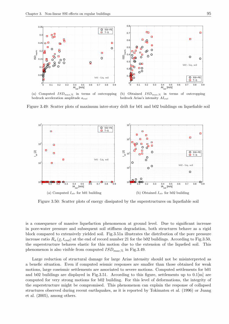
Chapter 3. Non-linear SSI effects on regular buildings 95
0 0.1 0.2 0.3 0.4 0.5 0.6 0.7 0.8 0.90
0.05
0.1
0.15
0.2
0.25
0.3
0.35
b01 - Liq. soil
AIout
[m/s]
ISD
max
%
SSI−FET−S
(a) Computed ISDmax,% in terms of outcroppingbedrock acceleration amplitude aout
0 0.1 0.2 0.3 0.4 0.5 0.6 0.7 0.8 0.90
0.1
0.2
0.3
0.4
0.5
0.6
0.7
0.8
b02 - Liq. soil
AIout
[m/s]
ISD
max
%
SSI−FET−S
(b) Obtained ISDmax,% in terms of outcroppingbedrock Arias’s intensity AIout
Figure 3.49: Scatter plots of maximum inter-story drift for b01 and b02 buildings on liquefiable soil
0 0.1 0.2 0.3 0.4 0.5 0.6 0.7 0.8 0.910
0
101
102
103
b01 - Liq. soil
IAout
[m/s]
I str [J
]
SSI−FET−S
(a) Computed Istr for b01 building
0 0.1 0.2 0.3 0.4 0.5 0.6 0.7 0.8 0.910
0
101
102
103
104
b02 - Liq. soil
IAout
[m/s]
I str [J
]
SSI−FET−S
(b) Obtained Istr for b02 building
Figure 3.50: Scatter plots of energy dissipated by the superstructures on liquefiable soil
is a consequence of massive liquefaction phenomenon at ground level. Due to significant increasein pore-water pressure and subsequent soil stiffness degradation, both structures behave as a rigidblock compared to extensively yielded soil. Fig.3.51a illustrates the distribution of the pore pressureincrease ratio Ru (x, tend) at the end of record number 21 for the b02 buildings. According to Fig.3.50,the superstructure behaves elastic for this motion due to the extension of the liquefied soil. Thisphenomenon is also visible from computed ISDmax,% in Fig.3.49.
Large reduction of structural damage for large Arias intensity should not be misinterpreted asa benefic situation. Even if computed seismic responses are smaller than those obtained for weakmotions, large coseismic settlements are associated to severe motions. Computed settlements for b01and b02 buildings are displayed in Fig.3.51. According to this figure, settlements up to 0.1[m] arecomputed for very strong motions for b02 building. For this level of deformations, the integrity ofthe superstructure might be compromised. This phenomenon can explain the response of collapsedstructures observed during recent earthquakes, as it is reported by Tokimatsu et al. (1996) or Juanget al. (2005), among others.
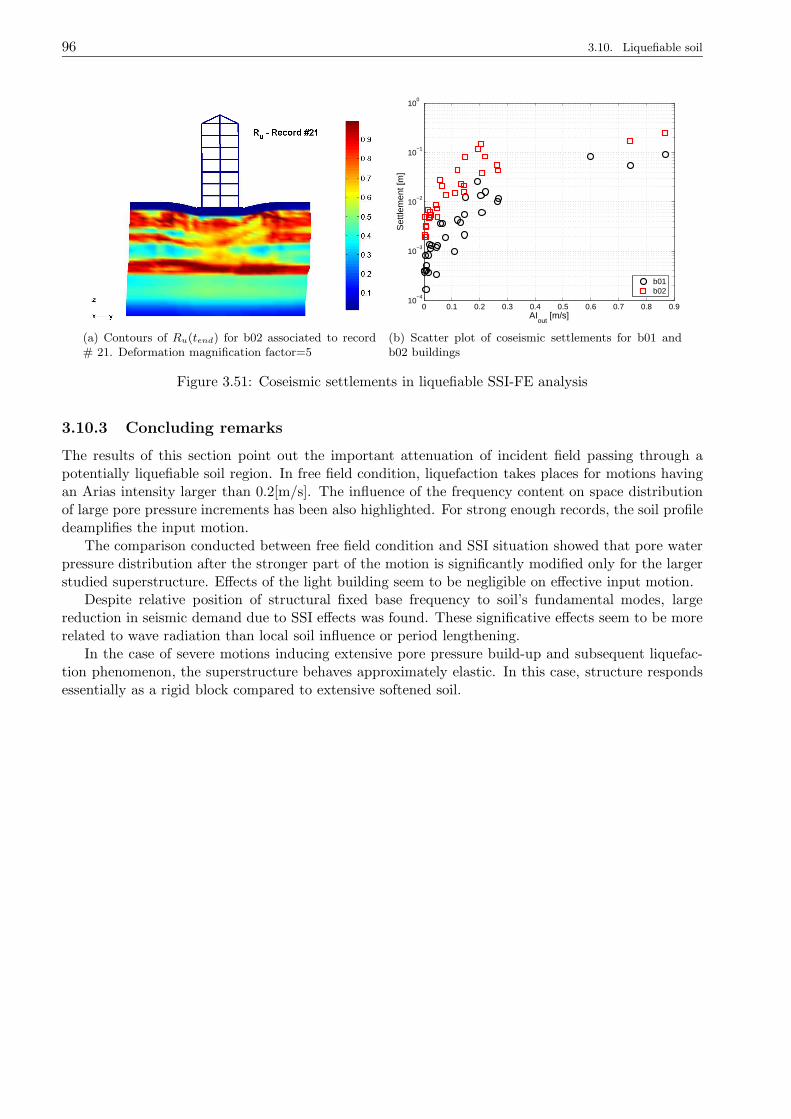
96 3.10. Liquefiable soil
(a) Contours of Ru(tend) for b02 associated to record# 21. Deformation magnification factor=5
0 0.1 0.2 0.3 0.4 0.5 0.6 0.7 0.8 0.910
−4
10−3
10−2
10−1
100
AIout
[m/s]
Set
tlem
ent [
m]
b01b02
(b) Scatter plot of coseismic settlements for b01 andb02 buildings
Figure 3.51: Coseismic settlements in liquefiable SSI-FE analysis
3.10.3 Concluding remarks
The results of this section point out the important attenuation of incident field passing through apotentially liquefiable soil region. In free field condition, liquefaction takes places for motions havingan Arias intensity larger than 0.2[m/s]. The influence of the frequency content on space distributionof large pore pressure increments has been also highlighted. For strong enough records, the soil profiledeamplifies the input motion.
The comparison conducted between free field condition and SSI situation showed that pore waterpressure distribution after the stronger part of the motion is significantly modified only for the largerstudied superstructure. Effects of the light building seem to be negligible on effective input motion.
Despite relative position of structural fixed base frequency to soil’s fundamental modes, largereduction in seismic demand due to SSI effects was found. These significative effects seem to be morerelated to wave radiation than local soil influence or period lengthening.
In the case of severe motions inducing extensive pore pressure build-up and subsequent liquefac-tion phenomenon, the superstructure behaves approximately elastic. In this case, structure respondsessentially as a rigid block compared to extensive softened soil.
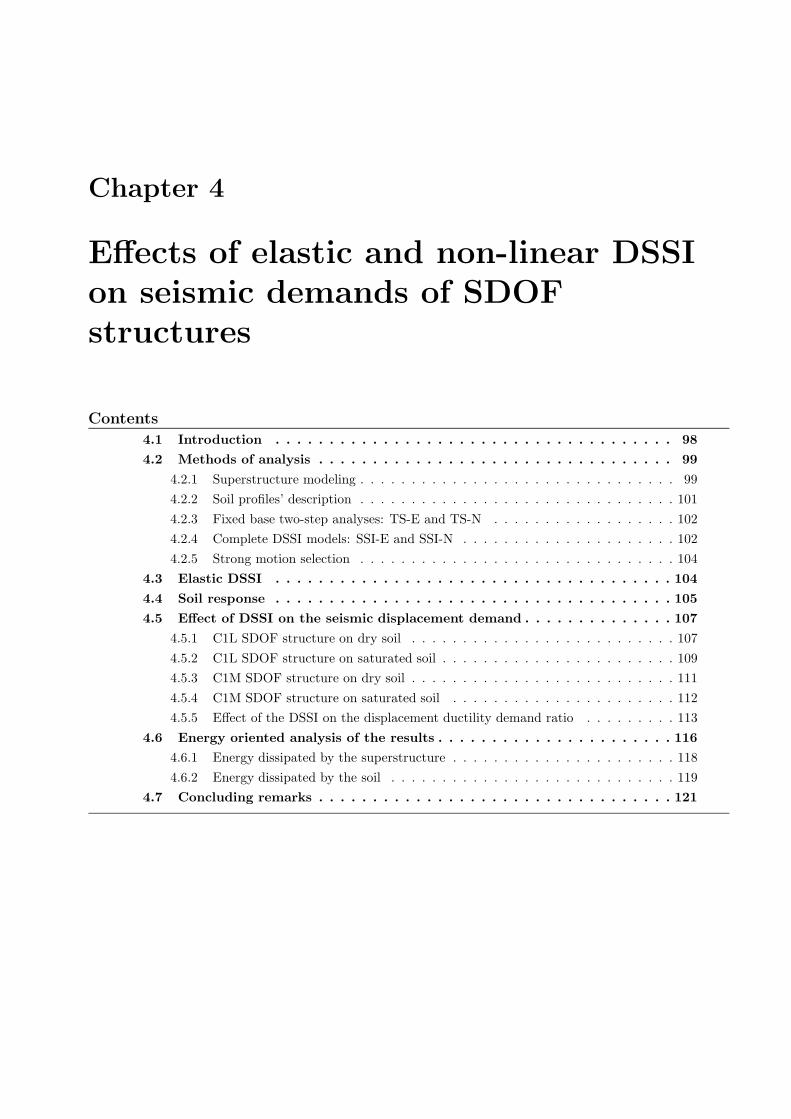
Chapter 4
Effects of elastic and non-linear DSSIon seismic demands of SDOFstructures
Contents
4.1 Introduction . . . . . . . . . . . . . . . . . . . . . . . . . . . . . . . . . . . . . 98
4.2 Methods of analysis . . . . . . . . . . . . . . . . . . . . . . . . . . . . . . . . . 99
4.2.1 Superstructure modeling . . . . . . . . . . . . . . . . . . . . . . . . . . . . . . . 99
4.2.2 Soil profiles’ description . . . . . . . . . . . . . . . . . . . . . . . . . . . . . . . 101
4.2.3 Fixed base two-step analyses: TS-E and TS-N . . . . . . . . . . . . . . . . . . 102
4.2.4 Complete DSSI models: SSI-E and SSI-N . . . . . . . . . . . . . . . . . . . . . 102
4.2.5 Strong motion selection . . . . . . . . . . . . . . . . . . . . . . . . . . . . . . . 104
4.3 Elastic DSSI . . . . . . . . . . . . . . . . . . . . . . . . . . . . . . . . . . . . . 104
4.4 Soil response . . . . . . . . . . . . . . . . . . . . . . . . . . . . . . . . . . . . . 105
4.5 Effect of DSSI on the seismic displacement demand . . . . . . . . . . . . . . 107
4.5.1 C1L SDOF structure on dry soil . . . . . . . . . . . . . . . . . . . . . . . . . . 107
4.5.2 C1L SDOF structure on saturated soil . . . . . . . . . . . . . . . . . . . . . . . 109
4.5.3 C1M SDOF structure on dry soil . . . . . . . . . . . . . . . . . . . . . . . . . . 111
4.5.4 C1M SDOF structure on saturated soil . . . . . . . . . . . . . . . . . . . . . . 112
4.5.5 Effect of the DSSI on the displacement ductility demand ratio . . . . . . . . . 113
4.6 Energy oriented analysis of the results . . . . . . . . . . . . . . . . . . . . . . 116
4.6.1 Energy dissipated by the superstructure . . . . . . . . . . . . . . . . . . . . . . 118
4.6.2 Energy dissipated by the soil . . . . . . . . . . . . . . . . . . . . . . . . . . . . 119
4.7 Concluding remarks . . . . . . . . . . . . . . . . . . . . . . . . . . . . . . . . . 121

98 4.1. Introduction
4.1 Introduction
The influence of the interaction of the soil with a superstructure on its dynamic behavior has beenthe subject of numerous investigations assuming linearity of both, superstructure and soil foundation.For elastic systems, first studies for soil-structure interacting systems were conducted by Jennings andBielak (1973); Veletsos and Meek (1974); Veletsos and Nair (1975) for surface-supported structures.In these works, the effects of the inertial DSSI are summarized by an equivalent SDOF characterizingsupport ground flexibility and the foundation damping. The effect of the flexible soil is included bymodifying the fixed base fundamental period. The foundation damping associated to radiation andsoil material damping is introduced by defining an effective damping of the superstructure-foundationsystem as the sum of a term proportional to viscous damping in the structure plus an equivalentviscous foundation damping. The increase of the natural period and the added foundation dampinghave been extensively studied by several authors (e.g Veletsos 1977; Luco 1980; Wolf 1985; Aviles andPerez-Rocha 1996). Nevertheless, this replacement oscillator approach is strictly valid only for elasticsuperstructure-foundation systems. This aspect is a significant limitation for earthquake engineering,where inelastic superstructure behavior is intentionally accepted. Despite the elastic intrinsic assump-tion, this approach has been included in several seismic design provisions (e.g. ATC 40 1996; FEMA356 2000; FEMA 450 2003), using free-field response spectra combined with effective values of both,fundamental period and equivalent viscous damping including elastic DSSI.
In principle, the effect of DSSI may differ between elastic and inelastic systems. Thus, the cur-rent interaction provisions based on elastic response studies could not be directly applicable to seismicdesign of typical buildings, expected to deform considerably beyond the yield limit during severe earth-quakes (Aviles and Perez-Rocha, 2003). According with the works of Veletsos (1977), the yielding ofthe superstructure can be viewed as a general increase of the relative flexibility between the super-structure and the soil, resulting into a reduction of DSSI effects. Unfortunately, the effects of the DSSIon yielding superstructure systems have not been extensively studied. Theoretical studies conductedby Priestley and Parck (1987) for elastoplastic bridge piers showed that the foundation compliancereduces the ductility capacity of the system. More recently, several other studies using the replacementoscillator technique (Ciampoli and Pinto, 1995; Rodriguez and Montes, 2000; Gazetas and Mylonakis,2001; Aviles and Perez-Rocha, 2003), have been conducted in order to elucidate the effect of the DSSIon the maximum required ductility. Similarly, Ghannad and Jahankhah (2007) use the replacementoscillator method to study the effect of DSSI on strength reduction factors of elastoplastic SDOFs.These studies point out some configurations were the DSSI has a considerable effect on the ductilitydemand of structures.
In the studies listed above, the soil replacement spring and dashpots are selected using frequency-independent approximations of the solutions available for dynamic impedances of rigid footings onelastic soil profiles, using Cone models, or using series of linear springs and dashpots attached tothe base foundation. Despite the used method, the numerical values of the soil replacement springand dashpot are dependent on the shear wave velocity. As shear wave velocity decreases when thesoil shear strain increases, some of these authors use degraded shear wave velocity values in theirmodels. Experimental results show that the limit of linear-elastic soil behavior is very low (γ < 10−5).This shear strain limit is normally exceeded during motions inducing damage of superstructures.Nevertheless, as described in Chapter 3, superstructure’s self weight increases the soil confinementunder the foundation reducing locally the energy dissipation by hysteresis. Indeed, larger soil energydissipation takes place in less confined zones. Consequently, the solely modification of the shearwave velocity under the foundation does not seem an appropriate approach to take into account thecontribution of the non-linear soil behavior.
Results presented in other chapters of this work highlight the effect of the combined DSSI effectsand non-linear soil behavior on the computed structural response, the separation of the contributionof each phenomenon to the total response is not easy to identify due to the complexity of the problem.This chapter describes the investigation conducted in order to compare the contribution of elastic andinelastic DSSI effects on the seismic response.
Chapter 4. Effects of elastic and non-linear DSSI on seismic demands of SDOF structures 99
4.2 Methods of analysis
In order to evaluate the contribution of the elastic DSSI in the modification of the structures’ dynamicresponse studied in previous chapters, two kinds of dynamic time-domain analyses are conducted:
1. Non-linear dynamic fixed base superstructure computations using as input motion the free fieldacceleration obtained for elastic (TS-E) and non-linear (TS-N) soil columns.
2. Complete dynamic soil-foundation-superstructure FE analyses, considering elastic (SSI-E) andnon-linear (SSI-N) soil behavior.
Both, TS-N and TS-E cases take into account non-linear structural behavior but neglect DSSIeffects. Complete DSSI analyses, SSI-E or SSI-N, include dynamic interaction effects and superstruc-ture material non-linearities. Details regarding each model, assumptions and parameters are providedin the following.
4.2.1 Superstructure modeling
The superstructures considered in this chapter are modeled by a massless continuous column (§1.3.2)of height h with a single mass m on top. The foundation is assumed square of side a (Fig.4.1a). Thesesuperstructures respond as a SDOF system with a fundamental period T0 in fixed-base condition.Damping is assumed to be hysteretic, controlled by the non-linear constitutive model of the column.Numerical values of properties characterizing each SDOF are selected on the basis of the classificationof building types used in HAZUS-MH MR3 (2003).
bmh
a a
b
b
(a) Schematic representation of superstructuremodel
D
A
Au
Du = µDy
Ay
Dy
Te
(b) Reference capacity curve according to HAZUS-MHMR3 (2003)
Figure 4.1: Superstructure’s SDOF representation and generic capacity curve
According to this document, reinforced concrete moment frame buildings can be classified, asshown in the first four columns of Tab.4.1, in terms of the total height and/or the number of stories.In this work, only C1L (low-rise) and C1M (mid-rise) categories are explored. In order to define thegeometric parameters describing the SDOFs, we start assuming a height. The typical height suggestedin Tab.4.1 is selected as height of the equivalent SDOF, i.e. 6 and 15[m], for low-rise and mid-risestructures, respectively. The choice of the foundation dimension a is based on the slender ratio h
a.
As usually the slender ratio increase with the number of stories of a building, we select slender ratiosof 1 and 1.5 for C1L and C1M categories, respectively. The total weight/mass is defined assuming anumber of levels and a uniform weight distribution of ρg = 10[kN/m3] over each level. Assuming 3and 5 levels, we obtain a total weight (mg) of 1080 and 5000[kN] for C1L and C1M, respectively.
In the HAZUS-MH MR3 (2003) methodology, some reference parameters are given to develop ca-pacity curves (Fig.4.1b). The value of these parameters depend on the conformity of the studied build-ing to modern seismic design provisions. In this way, four levels are defined: High-Code, Moderate-Code, Low-Code and Pre-Code. Last four columns of Tab.4.1 show the reference fundamental-mode

100 4.2. Methods of analysis
Table 4.1: Reinforced concrete moment frame classification and capacity parameters according toHAZUS-MH MR3 (2003)
Buildingtype
DescriptionStoriesrange
Typicalheight [m]
Te [s] Ay range [g] Au range [g] µ range
C1L Low-rise 1− 3 6 0.4 0.040−0.160 0.119−0.479 8− 5
C1M Mid-rise 4− 7 15.2 0.75 0.033−0.133 0.099−0.399 5.3−3.3
C1H High-rise 8+ 36.6 1.45 0.014−0.055 0.042−0.166 4− 2.5
period Te of the building depending on its type, the ranges of the control points of the fragility curveAy and Au and the range of ductility µ, defined by different seismic code conformity. In this table,Ay corresponds to the yield capacity representing the true lateral strength of the building and Au theultimate capacity when the system reaches the fully plastic state.
0 0.01 0.02 0.03 0.04 0.050
0.05
0.1
0.15
0.2
0.25T
0=0.4s
T0=0.75s
D [m]
A [g
]
Dy=0.0051m.
Ay=0.128g
Du=0.039m.
Au=0.219g
Dy=0.012m.
Ay=0.089g
Du=0.044m.
Au=0.163g
Figure 4.2: Computed capacity curves for C1L and C1M SDOFs
The provided value of Te is fixed as the target value for T0. The stiffness of the cantilever columnof the SDOF model (Fig.4.1a) is computed using the value of T0 and m, assuming a constant squaretransversal section and a fixed value of the Young modulus E. To model the post-yielding behavior,we use the constitutive model described in Appendix C. Thus, the values of the hardening modulus Etand initial yield stress σy are selected in order to obtain a capacity curve compatible with the rangesdefined in Tab.4.1. Parameters describing the used geometrical configuration and material propertiesare listed in Tab.4.2. The corresponding capacity curves are shown in Fig.4.2. It can be noticed thata maximum ductility µ of 7.6 and 3.7 are computed for C1L and C1M, respectively. These values,satisfy the ranges displayed in Tab.4.1 and correspond approximately to a Moderate-Code conformity.
Table 4.2: Properties of studied studied SDOFs
Label T0 [s] h [m] a [m] b [m] E [MPa] σy [MPa] Et [Pa]
C1L 0.40 6.0 6.0 0.98 25.5×10³ 6.0 0.1
C1M 0.75 15.0 10.0 2.09 25.5×10³ 5.5 0.1
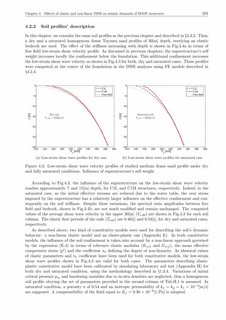
Chapter 4. Effects of elastic and non-linear DSSI on seismic demands of SDOF structures 101
4.2.2 Soil profiles’ description
In this chapter, we consider the same soil profiles as the previous chapter and described in §3.3.2. Thus,a dry and a saturated homogenous dense Toyoura sand profiles of 30[m] depth, overlying an elasticbedrock are used. The effect of the stiffness increasing with depth is shown in Fig.3.4a in terms offree field low-strain shear velocity profile. As discussed in previous chapters, the superstructure’s selfweight increases locally the confinement below the foundation. This additional confinement increasesthe low-strain shear wave velocity as shown in Fig.4.3 for both, dry and saturated cases. These profileswere computed at the center of the foundation in the DSSI analyses using FE models described in§4.2.4.
120 140 160 180 200 220 240 260 280 300−30
−25
−20
−15
−10
−5
0
Dry soilVs,30 = 233[m/s]
Vs [m/s]
z [m
]
C1LC1MFree field
(a) Low-strain shear wave profiles for dry case
120 140 160 180 200 220 240 260 280 300−30
−25
−20
−15
−10
−5
0
Saturated soilVs,30 = 204[m/s]
Vs [m/s]
z [m
]
C1LC1MFree field
(b) Low-strain shear wave profiles for saturated case
Figure 4.3: Low-strain shear wave velocity profiles of studied medium dense sand profile under dryand fully saturated conditions. Influence of superstructure’s self weight
According to Fig.4.3, the influence of the superstructure on the low-strain shear wave velocityreaches approximately 7 and 15[m] depth, for C1L and C1M structures, respectively. Indeed, in thesaturated case, as the initial effective stresses are reduced due to the water table, the over stressimposed by the superstructure has a relatively larger influence on the effective confinement and con-sequently on the soil stiffness. Despite these variations, the spectral ratio amplitudes between freefield and bedrock, shown in Fig.3.4b, are not much modified and remain unchanged. The computedvalues of the average shear wave velocity in the upper 30[m] (Vs,30) are shown in Fig.4.3 for each soilcolumn. The elastic first periods of the soils (Tsoil) are 0.46[s] and 0.54[s], for dry and saturated cases,respectively.
As described above, two kind of constitutive models were used for describing the soil’s dynamicbehavior: a non-linear elastic model and an elasto-plastic one (Appendix E). In both constitutivemodels, the influence of the soil confinement is taken into account by a non-linear approach governedby the expression (E.4) in terms of reference elastic modulus (Kref and Gref ), the mean effectivecompressive stress (p′) and the coefficient ne defining the degree of non-linearity. As identical valuesof elastic parameters and ne coefficient have been used for both constitutive models, the low-strainshear wave profiles shown in Fig.4.3 are valid for both cases. The parameters describing elasto-plastic constitutive model have been calibrated by simulating laboratory soil test (Appendix H) forboth dry and saturated condition, using the methodology described in §1.3.4. Variations of initialcritical pressure pc0 and hardening variables due to in-situ densities are neglected, thus a homogenoussoil profile obeying the set of parameters provided in the second column of Tab.H.1 is assumed. Insaturated condition, a porosity n of 0.54 and an isotropic permeability of kx = ky = kz = 10−4[m/s]are supposed. A compressibility of the fluid equal to Kf = 9.38 × 10⁻⁸[1/Pa] is adopted.
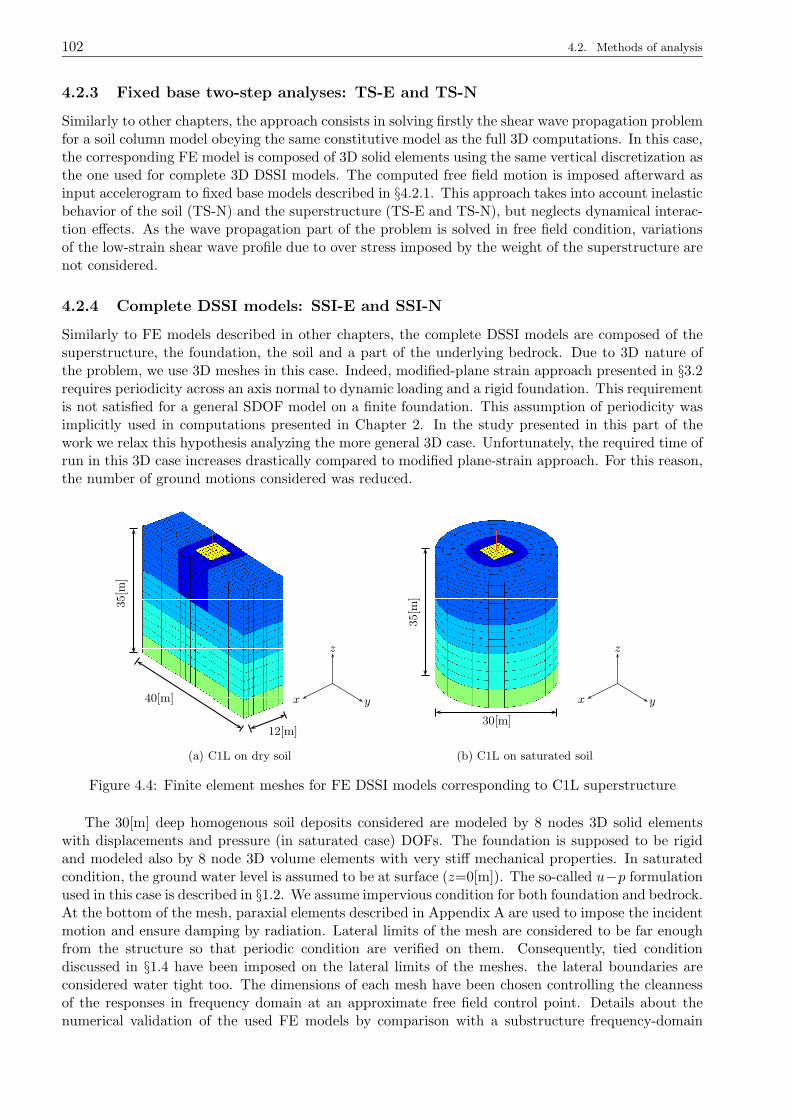
102 4.2. Methods of analysis
4.2.3 Fixed base two-step analyses: TS-E and TS-N
Similarly to other chapters, the approach consists in solving firstly the shear wave propagation problemfor a soil column model obeying the same constitutive model as the full 3D computations. In this case,the corresponding FE model is composed of 3D solid elements using the same vertical discretization asthe one used for complete 3D DSSI models. The computed free field motion is imposed afterward asinput accelerogram to fixed base models described in §4.2.1. This approach takes into account inelasticbehavior of the soil (TS-N) and the superstructure (TS-E and TS-N), but neglects dynamical interac-tion effects. As the wave propagation part of the problem is solved in free field condition, variationsof the low-strain shear wave profile due to over stress imposed by the weight of the superstructure arenot considered.
4.2.4 Complete DSSI models: SSI-E and SSI-N
Similarly to FE models described in other chapters, the complete DSSI models are composed of thesuperstructure, the foundation, the soil and a part of the underlying bedrock. Due to 3D nature ofthe problem, we use 3D meshes in this case. Indeed, modified-plane strain approach presented in §3.2requires periodicity across an axis normal to dynamic loading and a rigid foundation. This requirementis not satisfied for a general SDOF model on a finite foundation. This assumption of periodicity wasimplicitly used in computations presented in Chapter 2. In the study presented in this part of thework we relax this hypothesis analyzing the more general 3D case. Unfortunately, the required time ofrun in this 3D case increases drastically compared to modified plane-strain approach. For this reason,the number of ground motions considered was reduced.
z
yx40[m]
12[m]
35[m
]
(a) C1L on dry soil
z
yx
30[m]
35[m
]
(b) C1L on saturated soil
Figure 4.4: Finite element meshes for FE DSSI models corresponding to C1L superstructure
The 30[m] deep homogenous soil deposits considered are modeled by 8 nodes 3D solid elementswith displacements and pressure (in saturated case) DOFs. The foundation is supposed to be rigidand modeled also by 8 node 3D volume elements with very stiff mechanical properties. In saturatedcondition, the ground water level is assumed to be at surface (z=0[m]). The so-called u−p formulationused in this case is described in §1.2. We assume impervious condition for both foundation and bedrock.At the bottom of the mesh, paraxial elements described in Appendix A are used to impose the incidentmotion and ensure damping by radiation. Lateral limits of the mesh are considered to be far enoughfrom the structure so that periodic condition are verified on them. Consequently, tied conditiondiscussed in §1.4 have been imposed on the lateral limits of the meshes. the lateral boundaries areconsidered water tight too. The dimensions of each mesh have been chosen controlling the cleannessof the responses in frequency domain at an approximate free field control point. Details about thenumerical validation of the used FE models by comparison with a substructure frequency-domain
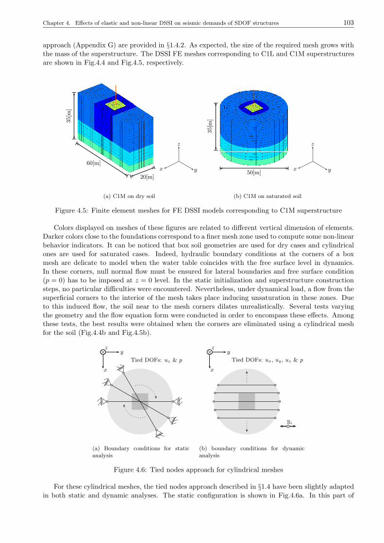
Chapter 4. Effects of elastic and non-linear DSSI on seismic demands of SDOF structures 103
approach (Appendix G) are provided in §1.4.2. As expected, the size of the required mesh grows withthe mass of the superstructure. The DSSI FE meshes corresponding to C1L and C1M superstructuresare shown in Fig.4.4 and Fig.4.5, respectively.
z
yx60[m]
20[m]
35[m
]
(a) C1M on dry soil
z
yx50[m]
35[m
]
(b) C1M on saturated soil
Figure 4.5: Finite element meshes for FE DSSI models corresponding to C1M superstructure
Colors displayed on meshes of these figures are related to different vertical dimension of elements.Darker colors close to the foundations correspond to a finer mesh zone used to compute some non-linearbehavior indicators. It can be noticed that box soil geometries are used for dry cases and cylindricalones are used for saturated cases. Indeed, hydraulic boundary conditions at the corners of a boxmesh are delicate to model when the water table coincides with the free surface level in dynamics.In these corners, null normal flow must be ensured for lateral boundaries and free surface condition(p = 0) has to be imposed at z = 0 level. In the static initialization and superstructure constructionsteps, no particular difficulties were encountered. Nevertheless, under dynamical load, a flow from thesuperficial corners to the interior of the mesh takes place inducing unsaturation in these zones. Dueto this induced flow, the soil near to the mesh corners dilates unrealistically. Several tests varyingthe geometry and the flow equation form were conducted in order to encompass these effects. Amongthese tests, the best results were obtained when the corners are eliminated using a cylindrical meshfor the soil (Fig.4.4b and Fig.4.5b).
y
x
×zTied DOFs: uz & p
(a) Boundary conditions for staticanalysis
y
x
×zTied DOFs: ux, uy , uz & p
ui×
(b) boundary conditions for dynamicanalysis
Figure 4.6: Tied nodes approach for cylindrical meshes
For these cylindrical meshes, the tied nodes approach described in §1.4 have been slightly adaptedin both static and dynamic analyses. The static configuration is shown in Fig.4.6a. In this part of
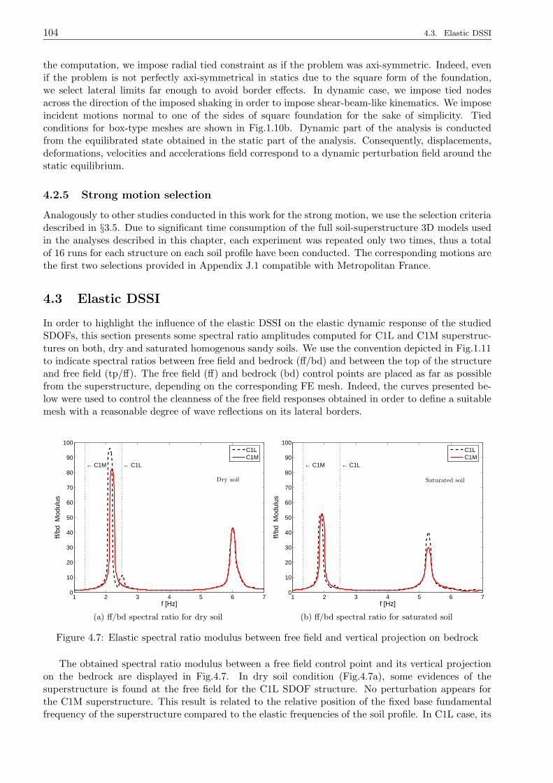
104 4.3. Elastic DSSI
the computation, we impose radial tied constraint as if the problem was axi-symmetric. Indeed, evenif the problem is not perfectly axi-symmetrical in statics due to the square form of the foundation,we select lateral limits far enough to avoid border effects. In dynamic case, we impose tied nodesacross the direction of the imposed shaking in order to impose shear-beam-like kinematics. We imposeincident motions normal to one of the sides of square foundation for the sake of simplicity. Tiedconditions for box-type meshes are shown in Fig.1.10b. Dynamic part of the analysis is conductedfrom the equilibrated state obtained in the static part of the analysis. Consequently, displacements,deformations, velocities and accelerations field correspond to a dynamic perturbation field around thestatic equilibrium.
4.2.5 Strong motion selection
Analogously to other studies conducted in this work for the strong motion, we use the selection criteriadescribed in §3.5. Due to significant time consumption of the full soil-superstructure 3D models usedin the analyses described in this chapter, each experiment was repeated only two times, thus a totalof 16 runs for each structure on each soil profile have been conducted. The corresponding motions arethe first two selections provided in Appendix J.1 compatible with Metropolitan France.
4.3 Elastic DSSI
In order to highlight the influence of the elastic DSSI on the elastic dynamic response of the studiedSDOFs, this section presents some spectral ratio amplitudes computed for C1L and C1M superstruc-tures on both, dry and saturated homogenous sandy soils. We use the convention depicted in Fig.1.11to indicate spectral ratios between free field and bedrock (ff/bd) and between the top of the structureand free field (tp/ff). The free field (ff) and bedrock (bd) control points are placed as far as possiblefrom the superstructure, depending on the corresponding FE mesh. Indeed, the curves presented be-low were used to control the cleanness of the free field responses obtained in order to define a suitablemesh with a reasonable degree of wave reflections on its lateral borders.
1 2 3 4 5 6 70
10
20
30
40
50
60
70
80
90
100
← C1M ← C1L
Dry soil
f [Hz]
ff/bd
Mod
ulus
C1LC1M
(a) ff/bd spectral ratio for dry soil
1 2 3 4 5 6 70
10
20
30
40
50
60
70
80
90
100
← C1M ← C1L
Saturated soil
f [Hz]
ff/bd
Mod
ulus
C1LC1M
(b) ff/bd spectral ratio for saturated soil
Figure 4.7: Elastic spectral ratio modulus between free field and vertical projection on bedrock
The obtained spectral ratio modulus between a free field control point and its vertical projectionon the bedrock are displayed in Fig.4.7. In dry soil condition (Fig.4.7a), some evidences of thesuperstructure is found at the free field for the C1L SDOF structure. No perturbation appears forthe C1M superstructure. This result is related to the relative position of the fixed base fundamentalfrequency of the superstructure compared to the elastic frequencies of the soil profile. In C1L case, its
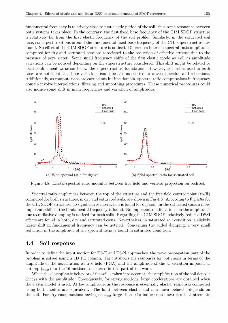
Chapter 4. Effects of elastic and non-linear DSSI on seismic demands of SDOF structures 105
fundamental frequency is relatively close to first elastic period of the soil, thus some resonance betweenboth systems takes place. In the contrary, the first fixed base frequency of the C1M SDOF structureis relatively far from the first elastic frequency of the soil profile. Similarly, in the saturated soilcase, some perturbations around the fundamental fixed base frequency of the C1L superstructure arefound. No effect of the C1M SDOF structure is noticed. Differences between spectral ratio amplitudescomputed for dry and saturated case are associated to the reduction of effective stresses due to thepresence of pore water. Some small frequency shifts of the first elastic mode as well as amplitudevariations can be noticed depending on the superstructure considered. This shift might be related tolocal confinement variation below the superstructure foundation. However, as meshes used in bothcases are not identical, these variations could be also associated to wave dispersion and reflections.Additionally, as computations are carried out in time domain, spectral ratio computations in frequencydomain involve interpolations, filtering and smoothing procedures. These numerical procedures couldalso induce some shift in main frequencies and variation of amplitudes.
1 2 3 4 5 60
10
20
30
40
50
60
C1L
f [Hz]
tp/ff
Mod
ulus
DrySaturatedFixed base
(a) ff/bd spectral ratio for dry soil
1 1.5 2 2.5 30
10
20
30
40
50
60
C1M
f [Hz]
tp/ff
Mod
ulus
DrySaturatedFixed base
(b) ff/bd spectral ratio for saturated soil
Figure 4.8: Elastic spectral ratio modulus between free field and vertical projection on bedrock
Spectral ratio amplitudes between the top of the structure and the free field control point (tp/ff)computed for both structures, in dry and saturated soils, are shown in Fig.4.8. According to Fig.4.8a forthe C1L SDOF structure, no significative interaction is found for dry soil. In the saturated case, a moreimportant shift in the fundamental frequency is found. No important modifications on the amplitudesdue to radiative damping is noticed for both soils. Regarding the C1M SDOF, relatively reduced DSSIeffects are found in both, dry and saturated cases. Nevertheless, in saturated soil condition, a slightlylarger shift in fundamental frequency can be noticed. Concerning the added damping, a very smallreduction in the amplitude of the spectral ratio is found in saturated condition.
4.4 Soil response
In order to define the input motion for TS-E and TS-N approaches, the wave propagation part of theproblem is solved using a 1D FE column. Fig.4.9 shows the responses for both soils in terms of theamplitude of the acceleration at free field (PGA) and the amplitude of the acceleration imposed atoutcrop (aout) for the 16 motions considered in this part of the work.
When the elastoplastic behavior of the soil is taken into account, the amplification of the soil depositdecays with the amplitude. Consequently, for strong motions, large accelerations are obtained whenthe elastic model is used. At low amplitude, as the response is essentially elastic, responses computedusing both models are equivalent. The limit between elastic and non-linear behavior depends onthe soil. For dry case, motions having an aout large than 0.1g induce non-linearities that attenuate
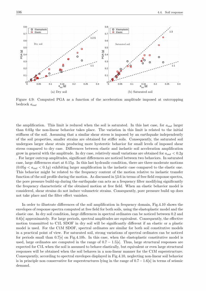
106 4.4. Soil response
0 0.05 0.1 0.15 0.2 0.25 0.30
0.1
0.2
0.3
0.4
0.5
0.6
0.7
0.8
Dry soil
1:1
1:2.5
aout
[g]
PG
A [g
]
ElastoplasticElastic
(a) Dry soil
0 0.05 0.1 0.15 0.2 0.25 0.30
0.1
0.2
0.3
0.4
0.5
0.6
0.7
0.8
Saturated soil
1:1
1:3
aout
[g]
PG
A [g
]
ElastoplasticElastic
(b) Saturated soil
Figure 4.9: Computed PGA as a function of the acceleration amplitude imposed at outcroppingbedrock aout
the amplification. This limit is reduced when the soil is saturated. In this last case, for aout largerthan 0.03g the non-linear behavior takes place. The variation in this limit is related to the initialstiffness of the soil. Assuming that a similar shear stress is imposed by an earthquake independentlyof the soil properties, smaller strains are obtained for stiffer soils. Consequently, the saturated soilundergoes larger shear strain producing more hysteretic behavior for small levels of imposed shearstress compared to dry case. Differences between elastic and inelastic soil acceleration amplificationgrow in general with the amplitude. In dry case, relatively small variations are obtained for aout < 0.2g. For larger outcrop amplitudes, significant differences are noticed between two behaviors. In saturatedcase, large differences start at 0.15g. In this last hydraulic condition, there are three moderate motions(0.05g < aout < 0.1g) exhibiting larger amplification in the inelastic case compared to the elastic one.This behavior might be related to the frequency content of the motion relative to inelastic transferfunction of the soil profile during the motion. As discussed in §3.6 in terms of free field response spectra,the pore pressure build-up during the earthquake can acts as a frequency filter modifying significantlythe frequency characteristic of the obtained motion at free field. When an elastic behavior model isconsidered, shear strains do not induce volumetric strains. Consequently, pore pressure build up doesnot take place and the filter effect vanishes.
In order to illustrate differences of the soil amplification in frequency domain, Fig.4.10 shows theenvelopes of response spectra computed at free field for both soils, using the elastoplastic model and theelastic one. In dry soil condition, large differences in spectral ordinates can be noticed between 0.2 and0.6[s] approximately. For large periods, spectral amplitudes are equivalent. Consequently, the effectivemotion transmitted to C1L SDOF in dry soil will be significantly different if an elastic or a plasticmodel is used. For the C1M SDOF, spectral ordinates are similar for both soil constitutive modelsin a practical point of view. For saturated soil, strong variations of spectral ordinates can be noticedfor periods small than 0.7[s] on Fig.4.10b. In this case, when the elastoplastic constitutive model isused, large ordinates are computed in the range of 0.7 − 1.5[s]. Thus, large structural responses areexpected for C1L when the soil is assumed to behave elastically, but equivalent or even large structuralresponses will be obtained when the soil behaves in a non-linear manner for the C1M superstructure.Consequently, according to spectral envelopes displayed in Fig.4.10, neglecting non-linear soil behavioris in principle non conservative for superstructures lying in the range of 0.7− 1.6[s] in terms of seismicdemand.
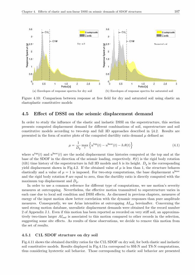
Chapter 4. Effects of elastic and non-linear DSSI on seismic demands of SDOF structures 107
(a) Envelopes of response spectra for dry soil (b) Envelopes of response spectra for saturated soil
Figure 4.10: Comparison between response at free field for dry and saturated soil using elastic anelastoplastic constitutive models
4.5 Effect of DSSI on the seismic displacement demand
In order to study the influence of the elastic and inelastic DSSI on the superstructure, this sectionpresents computed displacement demand for different combinations of soil, superstructure and soilconstitutive models according to two-step and full 3D approaches described in §4.2. Results arepresented in the form of scatter plots of the computed ductility ratio demand µ defined as:
µ =1
Dymaxt
utop(t)− ubase(t)− h.θ(t)
(4.1)
where utop(t) and ubase(t) are the nodal displacement time histories computed at the top and at thebase of the SDOF in the direction of the seismic loading, respectively. θ(t) is the rigid body rotation(tilt) time history of the superstructure in full 3D models and h is its height. Dy is the correspondingyield displacement shown in Fig.4.2. If the obtained value of µ is less than 1, the structure behaveselastically and a value of µ = 1 is imposed. For two-step computations, the base displacement ubase
and the rigid body rotation θ are equal to zero, thus the ductility ratio is directly computed with themaximum top displacement and Dy.
In order to use a common reference for different type of computations, we use motion’s severitymeasures at outcropping. Nevertheless, the effective motion transmitted to superstructure varies ineach case due to local soil condition and DSSI effects. As discussed in previous chapters, measures ofenergy of the input motion show better correlation with the dynamic responses than pure amplitudemeasures. Consequently, we use Arias intensities at outcropping AIout hereinafter. Concerning theused strong motion database, unrealistic displacement demands were obtained for the record number2 of Appendix J.1. Even if this motion has been reported as recorded on very stiff soil, an approxima-tively two-times larger AIout is associated to this motion compared to other records in the selection,suggesting some site effects. As results of these observations, we decide to remove this motion fromthe set of results.
4.5.1 C1L SDOF structure on dry soil
Fig.4.11 shows the obtained ductility ratios for the C1L SDOF on dry soil, for both elastic and inelasticsoil constitutive models. Results displayed in Fig.4.11a correspond to SSI-N and TS-N computations,thus considering hysteretic soil behavior. Those corresponding to elastic soil behavior are presented
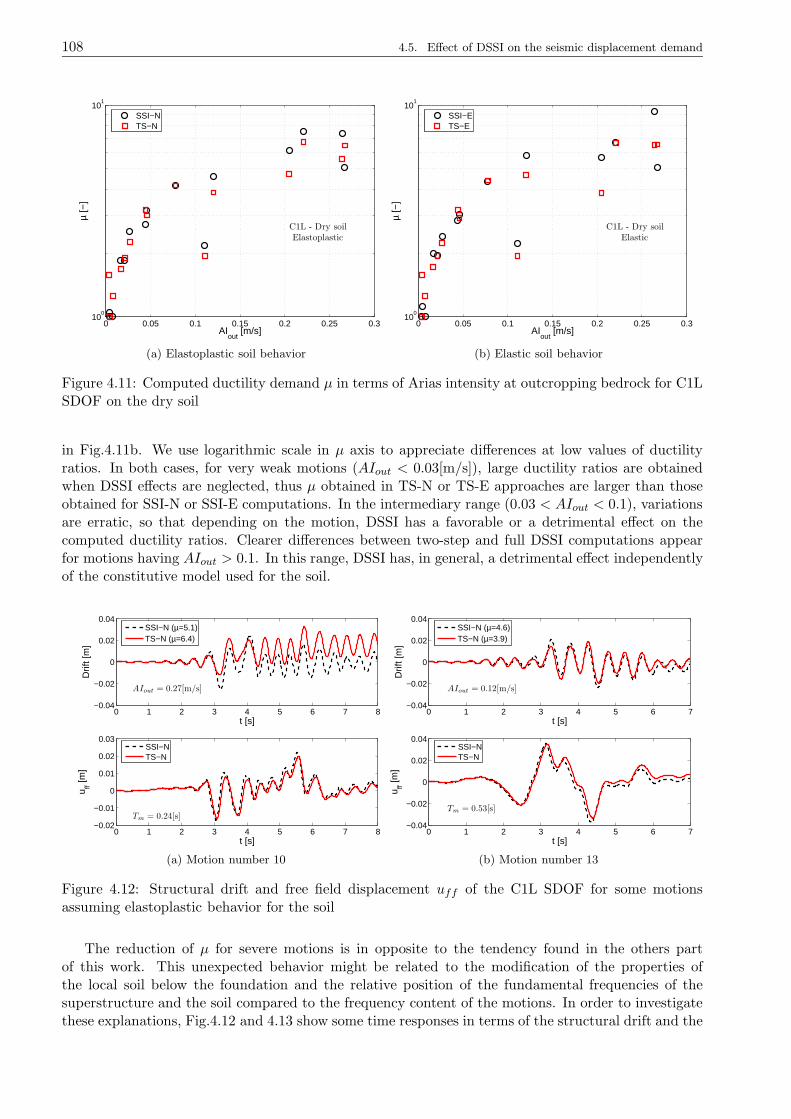
108 4.5. Effect of DSSI on the seismic displacement demand
0 0.05 0.1 0.15 0.2 0.25 0.310
0
101
C1L - Dry soilElastoplastic
AIout
[m/s]
µ [−
]
SSI−NTS−N
(a) Elastoplastic soil behavior
0 0.05 0.1 0.15 0.2 0.25 0.310
0
101
C1L - Dry soilElastic
AIout
[m/s]
µ [−
]
SSI−ETS−E
(b) Elastic soil behavior
Figure 4.11: Computed ductility demand µ in terms of Arias intensity at outcropping bedrock for C1LSDOF on the dry soil
in Fig.4.11b. We use logarithmic scale in µ axis to appreciate differences at low values of ductilityratios. In both cases, for very weak motions (AIout < 0.03[m/s]), large ductility ratios are obtainedwhen DSSI effects are neglected, thus µ obtained in TS-N or TS-E approaches are larger than thoseobtained for SSI-N or SSI-E computations. In the intermediary range (0.03 < AIout < 0.1), variationsare erratic, so that depending on the motion, DSSI has a favorable or a detrimental effect on thecomputed ductility ratios. Clearer differences between two-step and full DSSI computations appearfor motions having AIout > 0.1. In this range, DSSI has, in general, a detrimental effect independentlyof the constitutive model used for the soil.
0 1 2 3 4 5 6 7 8−0.04
−0.02
0
0.02
0.04
AIout = 0.27[m/s]
t [s]
Drif
t [m
]
SSI−N (µ=5.1)TS−N (µ=6.4)
0 1 2 3 4 5 6 7 8−0.02
−0.01
0
0.01
0.02
0.03
t [s]
Tm = 0.24[s]
u ff [m]
SSI−NTS−N
(a) Motion number 10
0 1 2 3 4 5 6 7−0.04
−0.02
0
0.02
0.04
AIout = 0.12[m/s]
t [s]
Drif
t [m
]
SSI−N (µ=4.6)TS−N (µ=3.9)
0 1 2 3 4 5 6 7−0.04
−0.02
0
0.02
0.04
t [s]
Tm = 0.53[s]
u ff [m]
SSI−NTS−N
(b) Motion number 13
Figure 4.12: Structural drift and free field displacement uff of the C1L SDOF for some motionsassuming elastoplastic behavior for the soil
The reduction of µ for severe motions is in opposite to the tendency found in the others partof this work. This unexpected behavior might be related to the modification of the properties ofthe local soil below the foundation and the relative position of the fundamental frequencies of thesuperstructure and the soil compared to the frequency content of the motions. In order to investigatethese explanations, Fig.4.12 and 4.13 show some time responses in terms of the structural drift and the

Chapter 4. Effects of elastic and non-linear DSSI on seismic demands of SDOF structures 109
free field displacement uff . We select two motions exhibiting opposite tendencies in terms of ductilityratio but having an AIout larger than 0.1[m/s]. The free field displacements are provided to controlthe clearness of the dynamic response of the complete 3D models.
0 1 2 3 4 5 6 7 8−0.04
−0.02
0
0.02
0.04
AIout = 0.27[m/s]
t [s]
Drif
t [m
]
SSI−E (µ=5.1)TS−E (µ=6.5)
0 1 2 3 4 5 6 7 8−0.02
−0.01
0
0.01
0.02
t [s]
Tm = 0.24[s]
u ff [m]
SSI−ETS−E
(a) Motion number 10
0 1 2 3 4 5 6 7−0.02
−0.01
0
0.01
0.02
0.03
AIout = 0.12[m/s]
t [s]
Drif
t [m
]
SSI−E (µ=5.8)TS−E (µ=4.7)
0 1 2 3 4 5 6 7−0.04
−0.02
0
0.02
0.04
t [s]
Tm = 0.53[s]
u ff [m]
SSI−ETS−E
(b) Motion number 13
Figure 4.13: Structural drift and free field displacement uff for some motions assuming elastic behaviorfor the soil. C1L SDOF
Fig.4.12 and 4.13 show the computed displacements for motions number 10 and 13 of Appendix J.1using elastoplastic and elastic soil constitutive models, respectively. For motion number 10, DSSI has afavorable effect, whereas DSSI has detrimental influence for motion number 13. For both motions, thecomputed free field displacement using a simple column (TS-N or TS-E) is similar to those obtained atfree field control points of the full 3D computations (SSI-N or SSI-E). Due to the severity of the motionnumber 10 (AIout = 0.27[m/s]), the soil undergoes plastic deformations when the elastoplastic model isconsidered. Comparing the free field response for this motion between SSI-N/TS-N and SSI-E/TS-E,a good agreement is in general found. However, the agreement is better in elastic cases. Consequently,when soil’s non-linear behavior is taken into account, some influence of the superstructure takes placeat free field control point. Similar conclusions can be derived for motion number 13. These effectsmight be reduced by increasing the size of the FE model with a consequent increase in the run timeconsumption, nevertheless free field responses seem accurate enough from a practical point of view.
Concerning the structural drift, responses are clearly different in Figs.4.12a and 4.13a when DSSIeffects are taken into account for motion number 10. In these figures, differences in the structuralresponse appear at 2.8[s] approximately. This effect appears independently of the adopted model forthe soil, suggesting a pure DSSI influence. In this time step of analysis, it seems that strong non-linearities take place in the superstructure modifying its subsequent dynamic response. Regarding themotion number 13, differences between fixed base computations and fully 3D models are visible mainlyin peaks of time-drift response. As the main period of the motion Tm = 0.53[s] is close to the firstelastic period of the soil of 0.46[s], these differences could be associated to some resonance betweenthe input and the soil neglected when the analysis is decoupled in two steps.
4.5.2 C1L SDOF structure on saturated soil
Results in terms of the computed ductility ratio following SSI-N/TS-N and SSI-E/TS-E approachesfor the saturated soil are shown in Fig.4.14. Similar tendency as the one observed in dry case can benoticed for very weak motions (AIout < 0.03[m/s]), thus a reduction of the computed ductility demandratio. As concerns the range 0.03 < AIout < 0.1[m/s], the responses are erratic, hence depending onthe motion an increase or a reduction in ductility demand is observed. For moderate to severe motion(AIout > 0.1[m/s]) different conclusions can be derived depending on the assumption taken for the soil
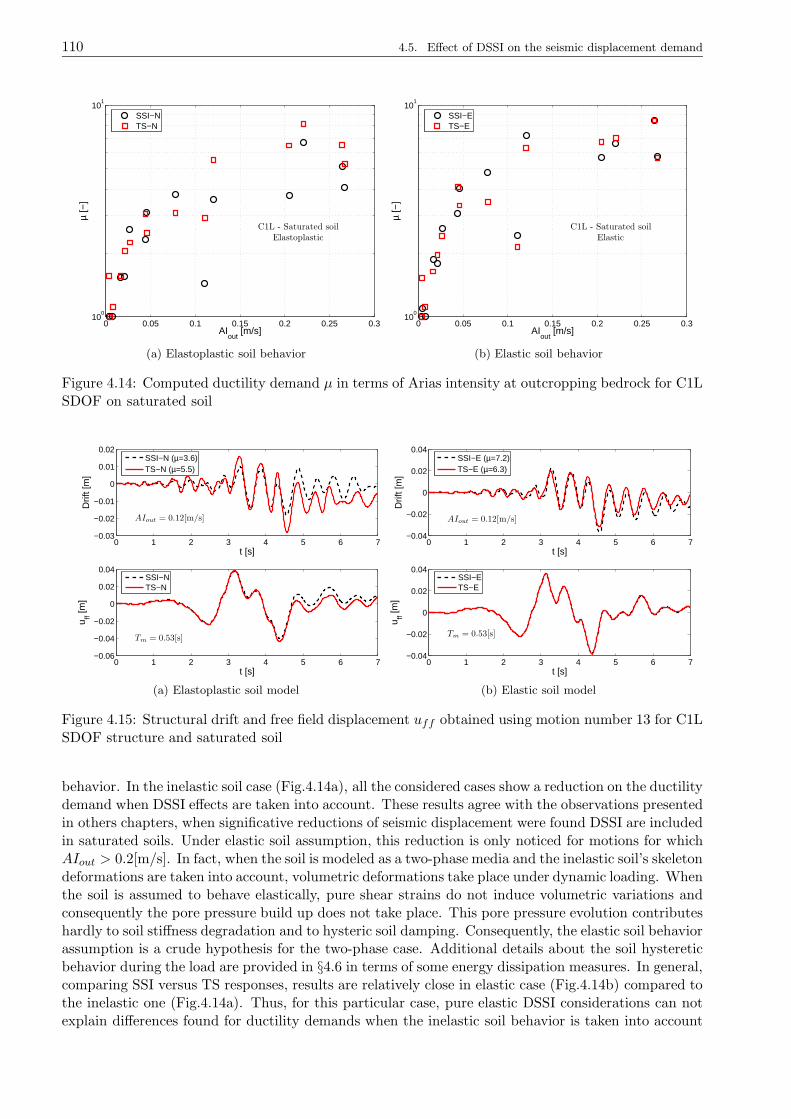
110 4.5. Effect of DSSI on the seismic displacement demand
0 0.05 0.1 0.15 0.2 0.25 0.310
0
101
C1L - Saturated soilElastoplastic
AIout
[m/s]
µ [−
]
SSI−NTS−N
(a) Elastoplastic soil behavior
0 0.05 0.1 0.15 0.2 0.25 0.310
0
101
C1L - Saturated soilElastic
AIout
[m/s]
µ [−
]
SSI−ETS−E
(b) Elastic soil behavior
Figure 4.14: Computed ductility demand µ in terms of Arias intensity at outcropping bedrock for C1LSDOF on saturated soil
0 1 2 3 4 5 6 7−0.03
−0.02
−0.01
0
0.01
0.02
AIout = 0.12[m/s]
t [s]
Drif
t [m
]
SSI−N (µ=3.6)TS−N (µ=5.5)
0 1 2 3 4 5 6 7−0.06
−0.04
−0.02
0
0.02
0.04
t [s]
Tm = 0.53[s]
u ff [m]
SSI−NTS−N
(a) Elastoplastic soil model
0 1 2 3 4 5 6 7−0.04
−0.02
0
0.02
0.04
AIout = 0.12[m/s]
t [s]
Drif
t [m
]
SSI−E (µ=7.2)TS−E (µ=6.3)
0 1 2 3 4 5 6 7−0.04
−0.02
0
0.02
0.04
t [s]
Tm = 0.53[s]
u ff [m]
SSI−ETS−E
(b) Elastic soil model
Figure 4.15: Structural drift and free field displacement uff obtained using motion number 13 for C1LSDOF structure and saturated soil
behavior. In the inelastic soil case (Fig.4.14a), all the considered cases show a reduction on the ductilitydemand when DSSI effects are taken into account. These results agree with the observations presentedin others chapters, when significative reductions of seismic displacement were found DSSI are includedin saturated soils. Under elastic soil assumption, this reduction is only noticed for motions for whichAIout > 0.2[m/s]. In fact, when the soil is modeled as a two-phase media and the inelastic soil’s skeletondeformations are taken into account, volumetric deformations take place under dynamic loading. Whenthe soil is assumed to behave elastically, pure shear strains do not induce volumetric variations andconsequently the pore pressure build up does not take place. This pore pressure evolution contributeshardly to soil stiffness degradation and to hysteric soil damping. Consequently, the elastic soil behaviorassumption is a crude hypothesis for the two-phase case. Additional details about the soil hystereticbehavior during the load are provided in §4.6 in terms of some energy dissipation measures. In general,comparing SSI versus TS responses, results are relatively close in elastic case (Fig.4.14b) compared tothe inelastic one (Fig.4.14a). Thus, for this particular case, pure elastic DSSI considerations can notexplain differences found for ductility demands when the inelastic soil behavior is taken into account
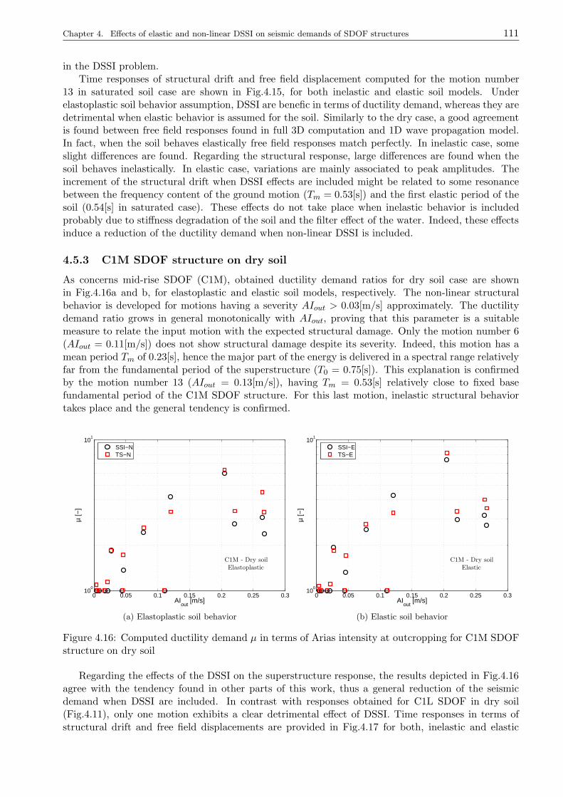
Chapter 4. Effects of elastic and non-linear DSSI on seismic demands of SDOF structures 111
in the DSSI problem.Time responses of structural drift and free field displacement computed for the motion number
13 in saturated soil case are shown in Fig.4.15, for both inelastic and elastic soil models. Underelastoplastic soil behavior assumption, DSSI are benefic in terms of ductility demand, whereas they aredetrimental when elastic behavior is assumed for the soil. Similarly to the dry case, a good agreementis found between free field responses found in full 3D computation and 1D wave propagation model.In fact, when the soil behaves elastically free field responses match perfectly. In inelastic case, someslight differences are found. Regarding the structural response, large differences are found when thesoil behaves inelastically. In elastic case, variations are mainly associated to peak amplitudes. Theincrement of the structural drift when DSSI effects are included might be related to some resonancebetween the frequency content of the ground motion (Tm = 0.53[s]) and the first elastic period of thesoil (0.54[s] in saturated case). These effects do not take place when inelastic behavior is includedprobably due to stiffness degradation of the soil and the filter effect of the water. Indeed, these effectsinduce a reduction of the ductility demand when non-linear DSSI is included.
4.5.3 C1M SDOF structure on dry soil
As concerns mid-rise SDOF (C1M), obtained ductility demand ratios for dry soil case are shownin Fig.4.16a and b, for elastoplastic and elastic soil models, respectively. The non-linear structuralbehavior is developed for motions having a severity AIout > 0.03[m/s] approximately. The ductilitydemand ratio grows in general monotonically with AIout, proving that this parameter is a suitablemeasure to relate the input motion with the expected structural damage. Only the motion number 6(AIout = 0.11[m/s]) does not show structural damage despite its severity. Indeed, this motion has amean period Tm of 0.23[s], hence the major part of the energy is delivered in a spectral range relativelyfar from the fundamental period of the superstructure (T0 = 0.75[s]). This explanation is confirmedby the motion number 13 (AIout = 0.13[m/s]), having Tm = 0.53[s] relatively close to fixed basefundamental period of the C1M SDOF structure. For this last motion, inelastic structural behaviortakes place and the general tendency is confirmed.
0 0.05 0.1 0.15 0.2 0.25 0.310
0
101
C1M - Dry soilElastoplastic
AIout
[m/s]
µ [−
]
SSI−NTS−N
(a) Elastoplastic soil behavior
0 0.05 0.1 0.15 0.2 0.25 0.310
0
101
C1M - Dry soilElastic
AIout
[m/s]
µ [−
]
SSI−ETS−E
(b) Elastic soil behavior
Figure 4.16: Computed ductility demand µ in terms of Arias intensity at outcropping for C1M SDOFstructure on dry soil
Regarding the effects of the DSSI on the superstructure response, the results depicted in Fig.4.16agree with the tendency found in other parts of this work, thus a general reduction of the seismicdemand when DSSI are included. In contrast with responses obtained for C1L SDOF in dry soil(Fig.4.11), only one motion exhibits a clear detrimental effect of DSSI. Time responses in terms ofstructural drift and free field displacements are provided in Fig.4.17 for both, inelastic and elastic
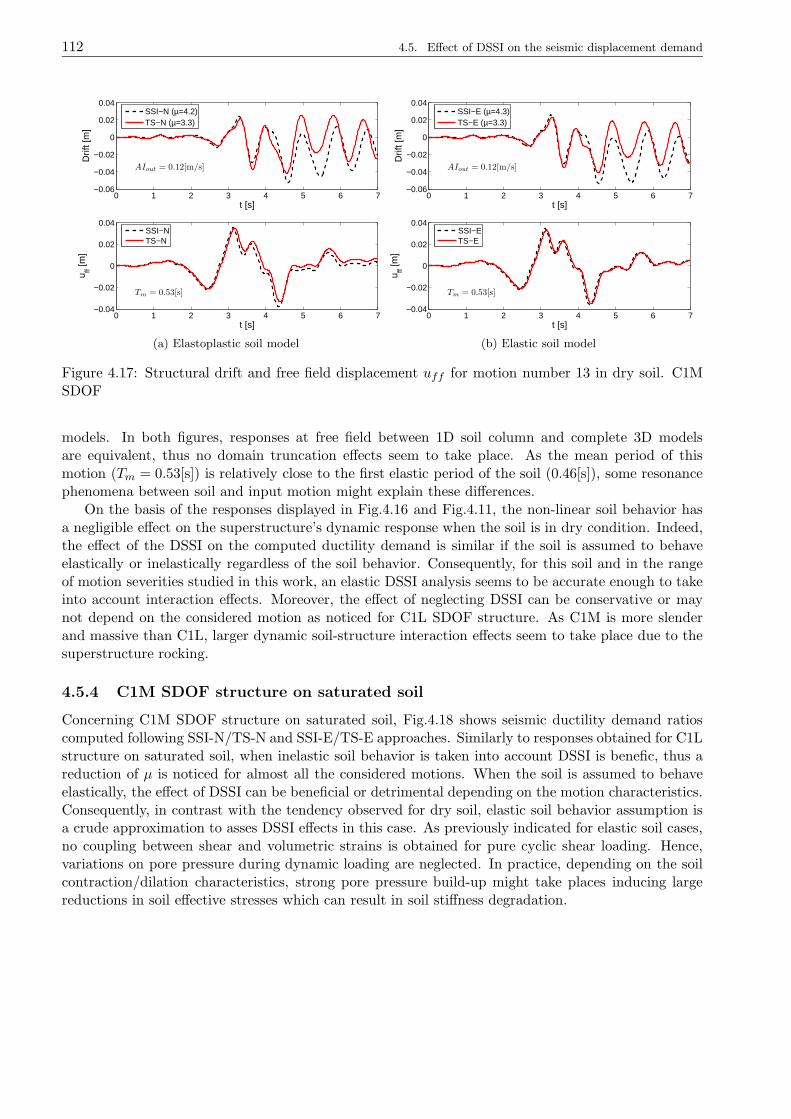
112 4.5. Effect of DSSI on the seismic displacement demand
0 1 2 3 4 5 6 7−0.06
−0.04
−0.02
0
0.02
0.04
AIout = 0.12[m/s]
t [s]
Drif
t [m
]
SSI−N (µ=4.2)TS−N (µ=3.3)
0 1 2 3 4 5 6 7−0.04
−0.02
0
0.02
0.04
t [s]
Tm = 0.53[s]
u ff [m]
SSI−NTS−N
(a) Elastoplastic soil model
0 1 2 3 4 5 6 7−0.06
−0.04
−0.02
0
0.02
0.04
AIout = 0.12[m/s]
t [s]
Drif
t [m
]
SSI−E (µ=4.3)TS−E (µ=3.3)
0 1 2 3 4 5 6 7−0.04
−0.02
0
0.02
0.04
t [s]
Tm = 0.53[s]
u ff [m]
SSI−ETS−E
(b) Elastic soil model
Figure 4.17: Structural drift and free field displacement uff for motion number 13 in dry soil. C1MSDOF
models. In both figures, responses at free field between 1D soil column and complete 3D modelsare equivalent, thus no domain truncation effects seem to take place. As the mean period of thismotion (Tm = 0.53[s]) is relatively close to the first elastic period of the soil (0.46[s]), some resonancephenomena between soil and input motion might explain these differences.
On the basis of the responses displayed in Fig.4.16 and Fig.4.11, the non-linear soil behavior hasa negligible effect on the superstructure’s dynamic response when the soil is in dry condition. Indeed,the effect of the DSSI on the computed ductility demand is similar if the soil is assumed to behaveelastically or inelastically regardless of the soil behavior. Consequently, for this soil and in the rangeof motion severities studied in this work, an elastic DSSI analysis seems to be accurate enough to takeinto account interaction effects. Moreover, the effect of neglecting DSSI can be conservative or maynot depend on the considered motion as noticed for C1L SDOF structure. As C1M is more slenderand massive than C1L, larger dynamic soil-structure interaction effects seem to take place due to thesuperstructure rocking.
4.5.4 C1M SDOF structure on saturated soil
Concerning C1M SDOF structure on saturated soil, Fig.4.18 shows seismic ductility demand ratioscomputed following SSI-N/TS-N and SSI-E/TS-E approaches. Similarly to responses obtained for C1Lstructure on saturated soil, when inelastic soil behavior is taken into account DSSI is benefic, thus areduction of µ is noticed for almost all the considered motions. When the soil is assumed to behaveelastically, the effect of DSSI can be beneficial or detrimental depending on the motion characteristics.Consequently, in contrast with the tendency observed for dry soil, elastic soil behavior assumption isa crude approximation to asses DSSI effects in this case. As previously indicated for elastic soil cases,no coupling between shear and volumetric strains is obtained for pure cyclic shear loading. Hence,variations on pore pressure during dynamic loading are neglected. In practice, depending on the soilcontraction/dilation characteristics, strong pore pressure build-up might take places inducing largereductions in soil effective stresses which can result in soil stiffness degradation.
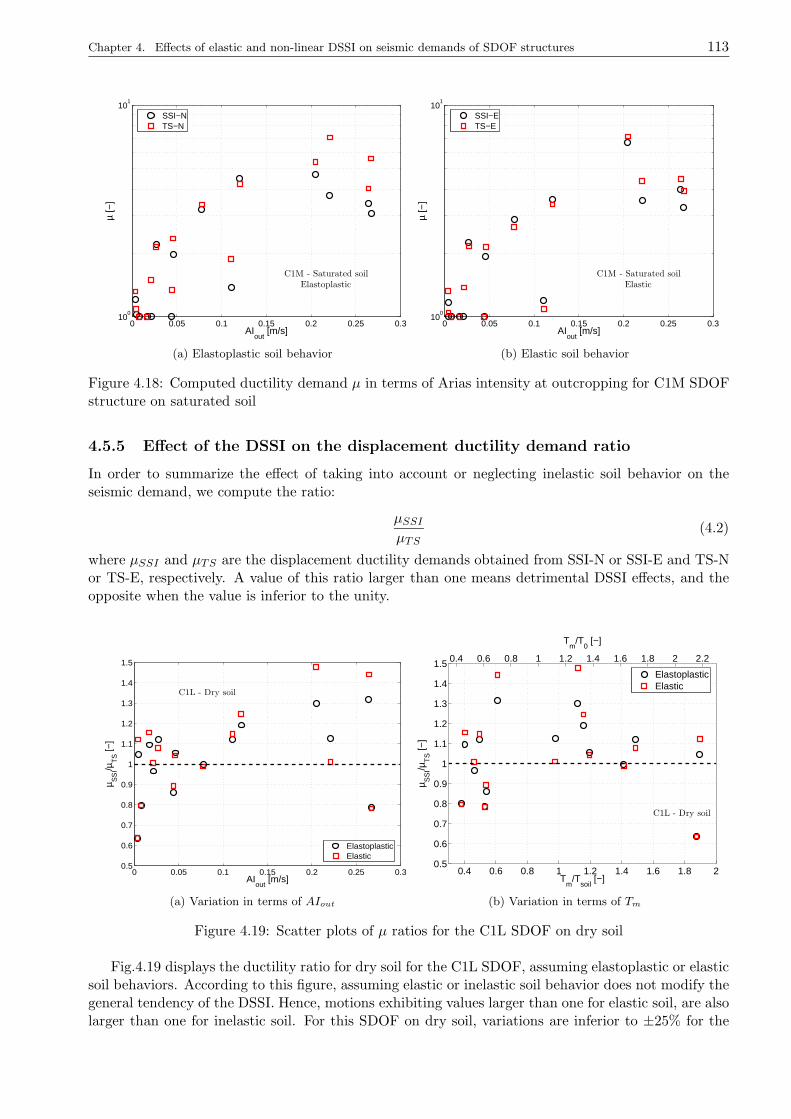
Chapter 4. Effects of elastic and non-linear DSSI on seismic demands of SDOF structures 113
0 0.05 0.1 0.15 0.2 0.25 0.310
0
101
C1M - Saturated soilElastoplastic
AIout
[m/s]
µ [−
]SSI−NTS−N
(a) Elastoplastic soil behavior
0 0.05 0.1 0.15 0.2 0.25 0.310
0
101
C1M - Saturated soilElastic
AIout
[m/s]
µ [−
]
SSI−ETS−E
(b) Elastic soil behavior
Figure 4.18: Computed ductility demand µ in terms of Arias intensity at outcropping for C1M SDOFstructure on saturated soil
4.5.5 Effect of the DSSI on the displacement ductility demand ratio
In order to summarize the effect of taking into account or neglecting inelastic soil behavior on theseismic demand, we compute the ratio:
µSSIµTS
(4.2)
where µSSI and µTS are the displacement ductility demands obtained from SSI-N or SSI-E and TS-Nor TS-E, respectively. A value of this ratio larger than one means detrimental DSSI effects, and theopposite when the value is inferior to the unity.
0 0.05 0.1 0.15 0.2 0.25 0.30.5
0.6
0.7
0.8
0.9
1
1.1
1.2
1.3
1.4
1.5
C1L - Dry soil
AIout
[m/s]
µ SS
I/µT
S [−
]
ElastoplasticElastic
(a) Variation in terms of AIout
0.4 0.6 0.8 1 1.2 1.4 1.6 1.8 2 2.2
Tm
/T0 [−]
0.4 0.6 0.8 1 1.2 1.4 1.6 1.8 20.5
0.6
0.7
0.8
0.9
1
1.1
1.2
1.3
1.4
1.5
C1L - Dry soil
Tm
/Tsoil
[−]
µ SS
I/µT
S [−
]
ElastoplasticElastic
(b) Variation in terms of Tm
Figure 4.19: Scatter plots of µ ratios for the C1L SDOF on dry soil
Fig.4.19 displays the ductility ratio for dry soil for the C1L SDOF, assuming elastoplastic or elasticsoil behaviors. According to this figure, assuming elastic or inelastic soil behavior does not modify thegeneral tendency of the DSSI. Hence, motions exhibiting values larger than one for elastic soil, are alsolarger than one for inelastic soil. For this SDOF on dry soil, variations are inferior to ±25% for the
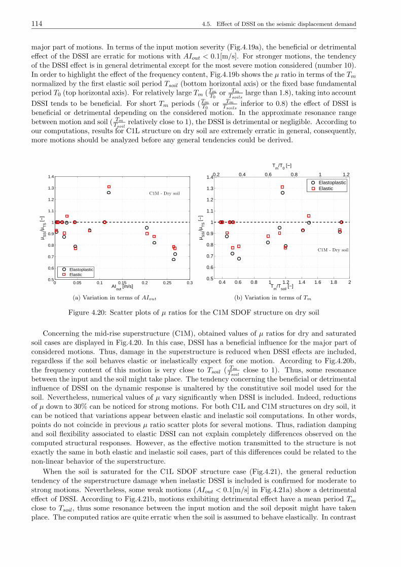
114 4.5. Effect of DSSI on the seismic displacement demand
major part of motions. In terms of the input motion severity (Fig.4.19a), the beneficial or detrimentaleffect of the DSSI are erratic for motions with AIout < 0.1[m/s]. For stronger motions, the tendencyof the DSSI effect is in general detrimental except for the most severe motion considered (number 10).In order to highlight the effect of the frequency content, Fig.4.19b shows the µ ratio in terms of the Tmnormalized by the first elastic soil period Tsoil (bottom horizontal axis) or the fixed base fundamentalperiod T0 (top horizontal axis). For relatively large Tm (Tm
T0or Tm
Tsoilslarge than 1.8), taking into account
DSSI tends to be beneficial. For short Tm periods (Tm
T0or Tm
Tsoilsinferior to 0.8) the effect of DSSI is
beneficial or detrimental depending on the considered motion. In the approximate resonance rangebetween motion and soil ( Tm
Tsoilrelatively close to 1), the DSSI is detrimental or negligible. According to
our computations, results for C1L structure on dry soil are extremely erratic in general, consequently,more motions should be analyzed before any general tendencies could be derived.
0 0.05 0.1 0.15 0.2 0.25 0.30.5
0.6
0.7
0.8
0.9
1
1.1
1.2
1.3
1.4
C1M - Dry soil
AIout
[m/s]
µ SS
I/µT
S [−
]
ElastoplasticElastic
(a) Variation in terms of AIout
0.2 0.4 0.6 0.8 1 1.2
Tm
/T0 [−]
0.4 0.6 0.8 1 1.2 1.4 1.6 1.8 20.5
0.6
0.7
0.8
0.9
1
1.1
1.2
1.3
1.4
C1M - Dry soil
Tm
/Tsoil
[−]
µ SS
I/µT
S [−
]
ElastoplasticElastic
(b) Variation in terms of Tm
Figure 4.20: Scatter plots of µ ratios for the C1M SDOF structure on dry soil
Concerning the mid-rise superstructure (C1M), obtained values of µ ratios for dry and saturatedsoil cases are displayed in Fig.4.20. In this case, DSSI has a beneficial influence for the major part ofconsidered motions. Thus, damage in the superstructure is reduced when DSSI effects are included,regardless if the soil behaves elastic or inelastically expect for one motion. According to Fig.4.20b,the frequency content of this motion is very close to Tsoil ( Tm
Tsoilclose to 1). Thus, some resonance
between the input and the soil might take place. The tendency concerning the beneficial or detrimentalinfluence of DSSI on the dynamic response is unaltered by the constitutive soil model used for thesoil. Nevertheless, numerical values of µ vary significantly when DSSI is included. Indeed, reductionsof µ down to 30% can be noticed for strong motions. For both C1L and C1M structures on dry soil, itcan be noticed that variations appear between elastic and inelastic soil computations. In other words,points do not coincide in previous µ ratio scatter plots for several motions. Thus, radiation dampingand soil flexibility associated to elastic DSSI can not explain completely differences observed on thecomputed structural responses. However, as the effective motion transmitted to the structure is notexactly the same in both elastic and inelastic soil cases, part of this differences could be related to thenon-linear behavior of the superstructure.
When the soil is saturated for the C1L SDOF structure case (Fig.4.21), the general reductiontendency of the superstructure damage when inelastic DSSI is included is confirmed for moderate tostrong motions. Nevertheless, some weak motions (AIout < 0.1[m/s] in Fig.4.21a) show a detrimentaleffect of DSSI. According to Fig.4.21b, motions exhibiting detrimental effect have a mean period Tmclose to Tsoil, thus some resonance between the input motion and the soil deposit might have takenplace. The computed ratios are quite erratic when the soil is assumed to behave elastically. In contrast
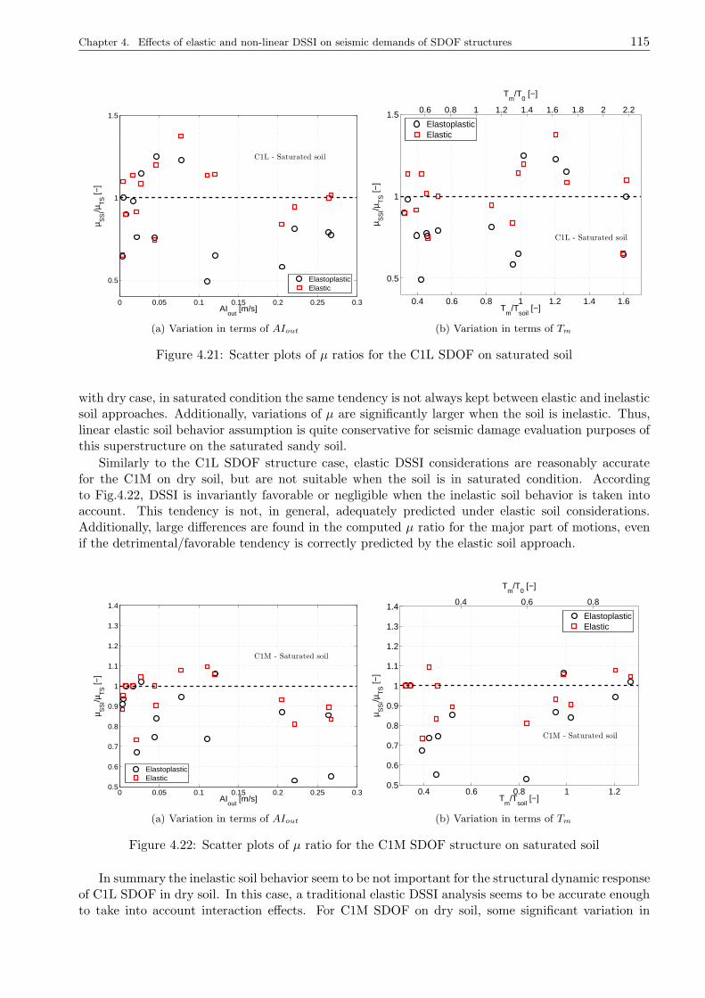
Chapter 4. Effects of elastic and non-linear DSSI on seismic demands of SDOF structures 115
0 0.05 0.1 0.15 0.2 0.25 0.3
0.5
1
1.5
C1L - Saturated soil
AIout
[m/s]
µ SS
I/µT
S [−
]
ElastoplasticElastic
(a) Variation in terms of AIout
0.6 0.8 1 1.2 1.4 1.6 1.8 2 2.2
Tm
/T0 [−]
0.4 0.6 0.8 1 1.2 1.4 1.6
0.5
1
1.5
C1L - Saturated soil
Tm
/Tsoil
[−]
µ SS
I/µT
S [−
]
ElastoplasticElastic
(b) Variation in terms of Tm
Figure 4.21: Scatter plots of µ ratios for the C1L SDOF on saturated soil
with dry case, in saturated condition the same tendency is not always kept between elastic and inelasticsoil approaches. Additionally, variations of µ are significantly larger when the soil is inelastic. Thus,linear elastic soil behavior assumption is quite conservative for seismic damage evaluation purposes ofthis superstructure on the saturated sandy soil.
Similarly to the C1L SDOF structure case, elastic DSSI considerations are reasonably accuratefor the C1M on dry soil, but are not suitable when the soil is in saturated condition. Accordingto Fig.4.22, DSSI is invariantly favorable or negligible when the inelastic soil behavior is taken intoaccount. This tendency is not, in general, adequately predicted under elastic soil considerations.Additionally, large differences are found in the computed µ ratio for the major part of motions, evenif the detrimental/favorable tendency is correctly predicted by the elastic soil approach.
0 0.05 0.1 0.15 0.2 0.25 0.30.5
0.6
0.7
0.8
0.9
1
1.1
1.2
1.3
1.4
C1M - Saturated soil
AIout
[m/s]
µ SS
I/µT
S [−
]
ElastoplasticElastic
(a) Variation in terms of AIout
0.4 0.6 0.8
Tm
/T0 [−]
0.4 0.6 0.8 1 1.20.5
0.6
0.7
0.8
0.9
1
1.1
1.2
1.3
1.4
C1M - Saturated soil
Tm
/Tsoil
[−]
µ SS
I/µT
S [−
]
ElastoplasticElastic
(b) Variation in terms of Tm
Figure 4.22: Scatter plots of µ ratio for the C1M SDOF structure on saturated soil
In summary the inelastic soil behavior seem to be not important for the structural dynamic responseof C1L SDOF in dry soil. In this case, a traditional elastic DSSI analysis seems to be accurate enoughto take into account interaction effects. For C1M SDOF on dry soil, some significant variation in
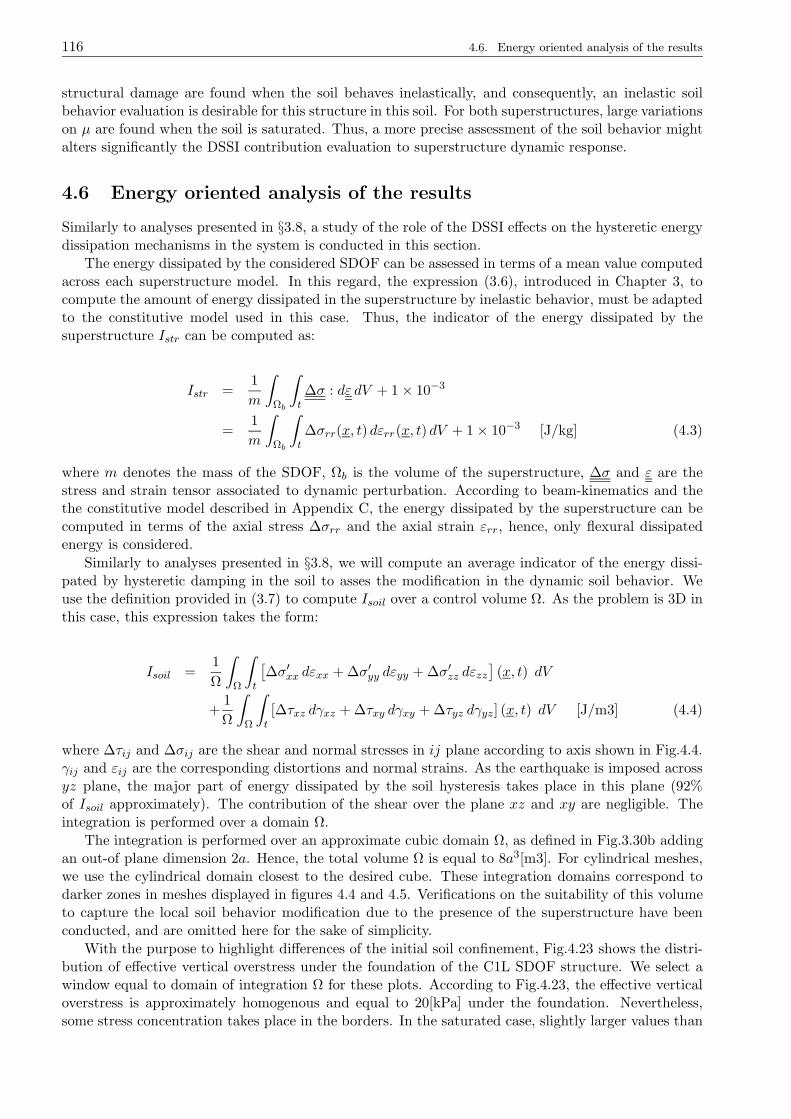
116 4.6. Energy oriented analysis of the results
structural damage are found when the soil behaves inelastically, and consequently, an inelastic soilbehavior evaluation is desirable for this structure in this soil. For both superstructures, large variationson µ are found when the soil is saturated. Thus, a more precise assessment of the soil behavior mightalters significantly the DSSI contribution evaluation to superstructure dynamic response.
4.6 Energy oriented analysis of the results
Similarly to analyses presented in §3.8, a study of the role of the DSSI effects on the hysteretic energydissipation mechanisms in the system is conducted in this section.
The energy dissipated by the considered SDOF can be assessed in terms of a mean value computedacross each superstructure model. In this regard, the expression (3.6), introduced in Chapter 3, tocompute the amount of energy dissipated in the superstructure by inelastic behavior, must be adaptedto the constitutive model used in this case. Thus, the indicator of the energy dissipated by thesuperstructure Istr can be computed as:
Istr =1
m
∫
Ωb
∫
t
∆σ : dε dV + 1× 10−3
=1
m
∫
Ωb
∫
t
∆σrr(x, t) dεrr(x, t) dV + 1× 10⁻³ [J/kg] (4.3)
where m denotes the mass of the SDOF, Ωb is the volume of the superstructure, ∆σ and ε are thestress and strain tensor associated to dynamic perturbation. According to beam-kinematics and thethe constitutive model described in Appendix C, the energy dissipated by the superstructure can becomputed in terms of the axial stress ∆σrr and the axial strain εrr, hence, only flexural dissipatedenergy is considered.
Similarly to analyses presented in §3.8, we will compute an average indicator of the energy dissi-pated by hysteretic damping in the soil to asses the modification in the dynamic soil behavior. Weuse the definition provided in (3.7) to compute Isoil over a control volume Ω. As the problem is 3D inthis case, this expression takes the form:
Isoil =1
Ω
∫
Ω
∫
t
[∆σ′xx dεxx + ∆σ′yy dεyy + ∆σ′zz dεzz
](x, t) dV
+1
Ω
∫
Ω
∫
t
[∆τxz dγxz + ∆τxy dγxy + ∆τyz dγyz] (x, t) dV [J/m3] (4.4)
where ∆τij and ∆σij are the shear and normal stresses in ij plane according to axis shown in Fig.4.4.γij and εij are the corresponding distortions and normal strains. As the earthquake is imposed acrossyz plane, the major part of energy dissipated by the soil hysteresis takes place in this plane (92%of Isoil approximately). The contribution of the shear over the plane xz and xy are negligible. Theintegration is performed over a domain Ω.
The integration is performed over an approximate cubic domain Ω, as defined in Fig.3.30b addingan out-of plane dimension 2a. Hence, the total volume Ω is equal to 8a3[m3]. For cylindrical meshes,we use the cylindrical domain closest to the desired cube. These integration domains correspond todarker zones in meshes displayed in figures 4.4 and 4.5. Verifications on the suitability of this volumeto capture the local soil behavior modification due to the presence of the superstructure have beenconducted, and are omitted here for the sake of simplicity.
With the purpose to highlight differences of the initial soil confinement, Fig.4.23 shows the distri-bution of effective vertical overstress under the foundation of the C1L SDOF structure. We select awindow equal to domain of integration Ω for these plots. According to Fig.4.23, the effective verticaloverstress is approximately homogenous and equal to 20[kPa] under the foundation. Nevertheless,some stress concentration takes place in the borders. In the saturated case, slightly larger values than
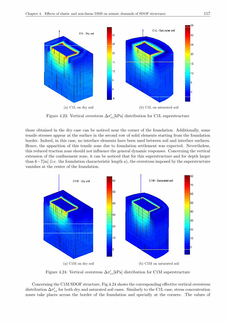
Chapter 4. Effects of elastic and non-linear DSSI on seismic demands of SDOF structures 117
(a) C1L on dry soil (b) C1L on saturated soil
Figure 4.23: Vertical overstress ∆σ′zz[kPa] distribution for C1L superstructure
those obtained in the dry case can be noticed near the corner of the foundation. Additionally, sometensile stresses appear at the surface in the second row of solid elements starting from the foundationborder. Indeed, in this case, no interface elements have been used between soil and interface surfaces.Hence, the apparition of this tensile zone due to foundation settlement was expected. Nevertheless,this reduced traction zone should not influence the general dynamic responses. Concerning the verticalextension of the confinement zone, it can be noticed that for this superstructure and for depth largerthan 6−7[m] (i.e. the foundation characteristic length a), the overstress imposed by the superstructurevanishes at the center of the foundation.
(a) C1M on dry soil (b) C1M on saturated soil
Figure 4.24: Vertical overstress ∆σ′zz[kPa] distribution for C1M superstructure
Concerning the C1M SDOF structure, Fig.4.24 shows the corresponding effective vertical overstressdistribution ∆σ′zz for both dry and saturated soil cases. Similarly to the C1L case, stress concentrationzones take places across the border of the foundation and specially at the corners. The values of
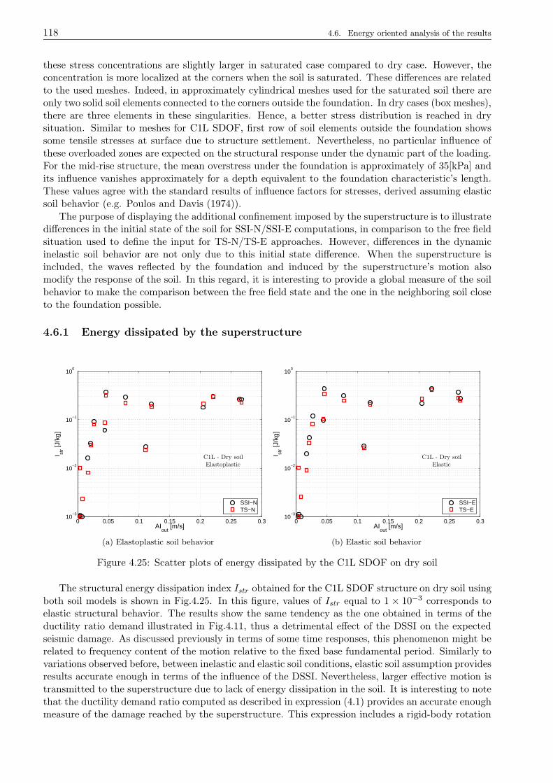
118 4.6. Energy oriented analysis of the results
these stress concentrations are slightly larger in saturated case compared to dry case. However, theconcentration is more localized at the corners when the soil is saturated. These differences are relatedto the used meshes. Indeed, in approximately cylindrical meshes used for the saturated soil there areonly two solid soil elements connected to the corners outside the foundation. In dry cases (box meshes),there are three elements in these singularities. Hence, a better stress distribution is reached in drysituation. Similar to meshes for C1L SDOF, first row of soil elements outside the foundation showssome tensile stresses at surface due to structure settlement. Nevertheless, no particular influence ofthese overloaded zones are expected on the structural response under the dynamic part of the loading.For the mid-rise structure, the mean overstress under the foundation is approximately of 35[kPa] andits influence vanishes approximately for a depth equivalent to the foundation characteristic’s length.These values agree with the standard results of influence factors for stresses, derived assuming elasticsoil behavior (e.g. Poulos and Davis (1974)).
The purpose of displaying the additional confinement imposed by the superstructure is to illustratedifferences in the initial state of the soil for SSI-N/SSI-E computations, in comparison to the free fieldsituation used to define the input for TS-N/TS-E approaches. However, differences in the dynamicinelastic soil behavior are not only due to this initial state difference. When the superstructure isincluded, the waves reflected by the foundation and induced by the superstructure’s motion alsomodify the response of the soil. In this regard, it is interesting to provide a global measure of the soilbehavior to make the comparison between the free field state and the one in the neighboring soil closeto the foundation possible.
4.6.1 Energy dissipated by the superstructure
0 0.05 0.1 0.15 0.2 0.25 0.310
−3
10−2
10−1
100
C1L - Dry soilElastoplastic
AIout
[m/s]
I str [J
/kg]
SSI−NTS−N
(a) Elastoplastic soil behavior
0 0.05 0.1 0.15 0.2 0.25 0.310
−3
10−2
10−1
100
C1L - Dry soilElastic
AIout
[m/s]
I str [J
/kg]
SSI−ETS−E
(b) Elastic soil behavior
Figure 4.25: Scatter plots of energy dissipated by the C1L SDOF on dry soil
The structural energy dissipation index Istr obtained for the C1L SDOF structure on dry soil usingboth soil models is shown in Fig.4.25. In this figure, values of Istr equal to 1 × 10⁻³ corresponds toelastic structural behavior. The results show the same tendency as the one obtained in terms of theductility ratio demand illustrated in Fig.4.11, thus a detrimental effect of the DSSI on the expectedseismic damage. As discussed previously in terms of some time responses, this phenomenon might berelated to frequency content of the motion relative to the fixed base fundamental period. Similarly tovariations observed before, between inelastic and elastic soil conditions, elastic soil assumption providesresults accurate enough in terms of the influence of the DSSI. Nevertheless, larger effective motion istransmitted to the superstructure due to lack of energy dissipation in the soil. It is interesting to notethat the ductility demand ratio computed as described in expression (4.1) provides an accurate enoughmeasure of the damage reached by the superstructure. This expression includes a rigid-body rotation
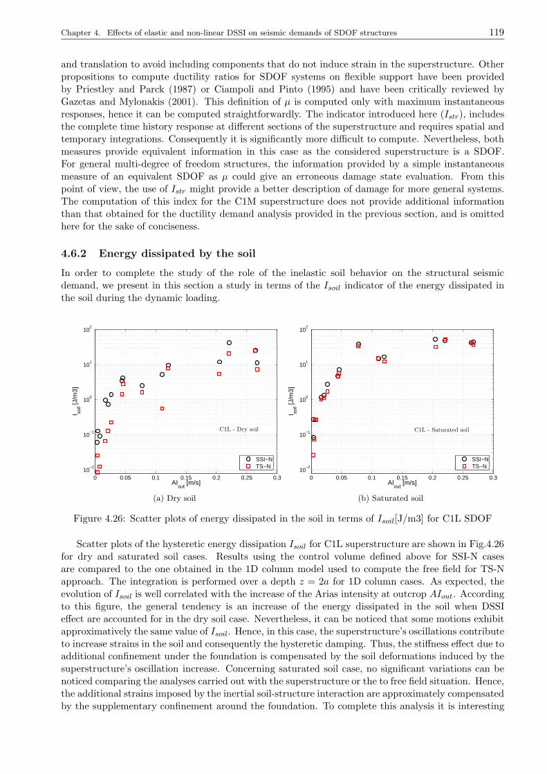
Chapter 4. Effects of elastic and non-linear DSSI on seismic demands of SDOF structures 119
and translation to avoid including components that do not induce strain in the superstructure. Otherpropositions to compute ductility ratios for SDOF systems on flexible support have been providedby Priestley and Parck (1987) or Ciampoli and Pinto (1995) and have been critically reviewed byGazetas and Mylonakis (2001). This definition of µ is computed only with maximum instantaneousresponses, hence it can be computed straightforwardly. The indicator introduced here (Istr), includesthe complete time history response at different sections of the superstructure and requires spatial andtemporary integrations. Consequently it is significantly more difficult to compute. Nevertheless, bothmeasures provide equivalent information in this case as the considered superstructure is a SDOF.For general multi-degree of freedom structures, the information provided by a simple instantaneousmeasure of an equivalent SDOF as µ could give an erroneous damage state evaluation. From thispoint of view, the use of Istr might provide a better description of damage for more general systems.The computation of this index for the C1M superstructure does not provide additional informationthan that obtained for the ductility demand analysis provided in the previous section, and is omittedhere for the sake of conciseness.
4.6.2 Energy dissipated by the soil
In order to complete the study of the role of the inelastic soil behavior on the structural seismicdemand, we present in this section a study in terms of the Isoil indicator of the energy dissipated inthe soil during the dynamic loading.
0 0.05 0.1 0.15 0.2 0.25 0.310
−2
10−1
100
101
102
C1L - Dry soil
AIout
[m/s]
I soil [J
/m3]
SSI−NTS−N
(a) Dry soil
0 0.05 0.1 0.15 0.2 0.25 0.310
−2
10−1
100
101
102
C1L - Saturated soil
AIout
[m/s]
I soil [J
/m3]
SSI−NTS−N
(b) Saturated soil
Figure 4.26: Scatter plots of energy dissipated in the soil in terms of Isoil[J/m3] for C1L SDOF
Scatter plots of the hysteretic energy dissipation Isoil for C1L superstructure are shown in Fig.4.26for dry and saturated soil cases. Results using the control volume defined above for SSI-N casesare compared to the one obtained in the 1D column model used to compute the free field for TS-Napproach. The integration is performed over a depth z = 2a for 1D column cases. As expected, theevolution of Isoil is well correlated with the increase of the Arias intensity at outcrop AIout. Accordingto this figure, the general tendency is an increase of the energy dissipated in the soil when DSSIeffect are accounted for in the dry soil case. Nevertheless, it can be noticed that some motions exhibitapproximatively the same value of Isoil. Hence, in this case, the superstructure’s oscillations contributeto increase strains in the soil and consequently the hysteretic damping. Thus, the stiffness effect due toadditional confinement under the foundation is compensated by the soil deformations induced by thesuperstructure’s oscillation increase. Concerning saturated soil case, no significant variations can benoticed comparing the analyses carried out with the superstructure or the to free field situation. Hence,the additional strains imposed by the inertial soil-structure interaction are approximately compensatedby the supplementary confinement around the foundation. To complete this analysis it is interesting
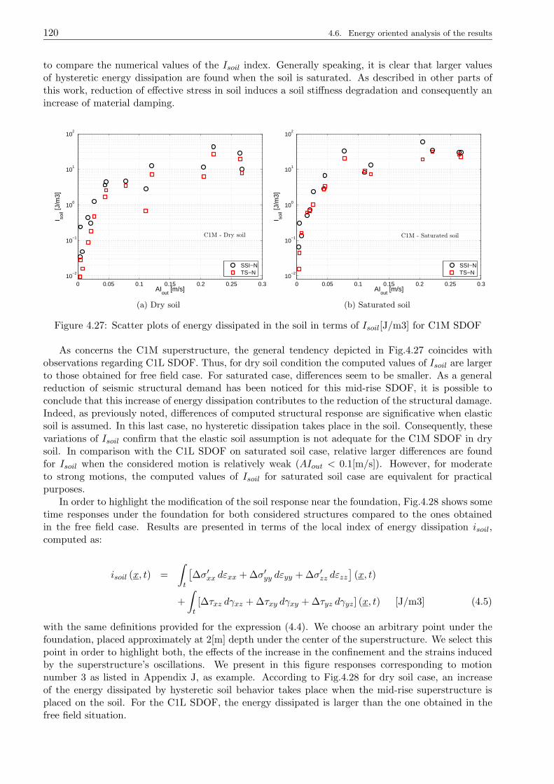
120 4.6. Energy oriented analysis of the results
to compare the numerical values of the Isoil index. Generally speaking, it is clear that larger valuesof hysteretic energy dissipation are found when the soil is saturated. As described in other parts ofthis work, reduction of effective stress in soil induces a soil stiffness degradation and consequently anincrease of material damping.
0 0.05 0.1 0.15 0.2 0.25 0.310
−2
10−1
100
101
102
C1M - Dry soil
AIout
[m/s]
I soil [J
/m3]
SSI−NTS−N
(a) Dry soil
0 0.05 0.1 0.15 0.2 0.25 0.310
−2
10−1
100
101
102
C1M - Saturated soil
AIout
[m/s]
I soil [J
/m3]
SSI−NTS−N
(b) Saturated soil
Figure 4.27: Scatter plots of energy dissipated in the soil in terms of Isoil[J/m3] for C1M SDOF
As concerns the C1M superstructure, the general tendency depicted in Fig.4.27 coincides withobservations regarding C1L SDOF. Thus, for dry soil condition the computed values of Isoil are largerto those obtained for free field case. For saturated case, differences seem to be smaller. As a generalreduction of seismic structural demand has been noticed for this mid-rise SDOF, it is possible toconclude that this increase of energy dissipation contributes to the reduction of the structural damage.Indeed, as previously noted, differences of computed structural response are significative when elasticsoil is assumed. In this last case, no hysteretic dissipation takes place in the soil. Consequently, thesevariations of Isoil confirm that the elastic soil assumption is not adequate for the C1M SDOF in drysoil. In comparison with the C1L SDOF on saturated soil case, relative larger differences are foundfor Isoil when the considered motion is relatively weak (AIout < 0.1[m/s]). However, for moderateto strong motions, the computed values of Isoil for saturated soil case are equivalent for practicalpurposes.
In order to highlight the modification of the soil response near the foundation, Fig.4.28 shows sometime responses under the foundation for both considered structures compared to the ones obtainedin the free field case. Results are presented in terms of the local index of energy dissipation isoil,computed as:
isoil (x, t) =
∫
t
[∆σ′xx dεxx + ∆σ′yy dεyy + ∆σ′zz dεzz
](x, t)
+
∫
t
[∆τxz dγxz + ∆τxy dγxy + ∆τyz dγyz] (x, t) [J/m3] (4.5)
with the same definitions provided for the expression (4.4). We choose an arbitrary point under thefoundation, placed approximately at 2[m] depth under the center of the superstructure. We select thispoint in order to highlight both, the effects of the increase in the confinement and the strains inducedby the superstructure’s oscillations. We present in this figure responses corresponding to motionnumber 3 as listed in Appendix J, as example. According to Fig.4.28 for dry soil case, an increaseof the energy dissipated by hysteretic soil behavior takes place when the mid-rise superstructure isplaced on the soil. For the C1L SDOF, the energy dissipated is larger than the one obtained in thefree field situation.

Chapter 4. Effects of elastic and non-linear DSSI on seismic demands of SDOF structures 121
0 5 10 15 20 25−0.2
0
0.2
0.4
0.6
0.8
1
1.2
1.4
1.6Motion # 3Tm = 0.65[s]
AIout = 0.078[m/s]
Dry soil atx =0.21[m], y=0.21[m] and z=-1.8[m]
t [s]
i soil [J
/m3]
Free fieldC1LC1M
(a) Dry soil
0 5 10 15 20 25−2
0
2
4
6
8
10
12
14
Motion # 3Tm = 0.65[s]
AIout = 0.078[m/s]
Saturated soil atx =0.26[m], y=0.26[m] and z=-1.8[m]
t [s]
i soil [J
/m3]
Free fieldC1LC1M
(b) Saturated soil
Figure 4.28: isoil evolution at 2[m] depth under the center of foundation for two motions
The tendency is completely inverted for the saturated case shown in Fig.4.28b. In fact, in this case,due to reduction of effective stresses, larger values of isoil are found for the free field case compared tothe DSSI models. At 2[m] depth, large confinement provided by the mid-rise SDOF structure increasessignificantly the soil stiffness compared to the free field or the C1L structure model, and consequentlyreduces the induced shear strains and energy dissipation. Indeed, at free field the situation is close toliquefaction, and locally the induced hysteretic damping grows drastically. Nevertheless this situationis local, the averaged effect over the control volume Ω has been shown in previous figures. However,the implications of this local effects can be important in terms of settlements as discussed in §3.10.2.2.The purpose of introducing this energy analysis was to complete the description of the superstructureresponses in order to relate detected variations with the soil inelastic state. In this regard, increases inhysteretic damping highlighted for mid-rise SDOF structure in both dry and saturated soil cases, mightexplain general reduction of expected structural damage. Concerning the low-rise SDOF structure,results shown in this section suggest that DSSI effects are fundamentally elastic in dry case, and onlyin saturated case an influence of inelastic soil behavior is clear.
4.7 Concluding remarks
This chapter was devoted to identify the contribution of the inelastic soil behavior to the generalnon-linear DSSI problem. With this purpose, a comparative analysis between elastic and inelastic soilbehavior assumptions was presented. In order to make as general as possible our results, we selectedtwo generic SDOF structures taking generic values suggested in some design codes. As the generalproblem of a shallow rigid foundation with SDOF structure is essentially three-dimensional, we used3D FE models to analyze this problem. A homogenous medium dense sand soil profile in two hydraulicconditions (dry and saturated) has been used.
The results point out that, in general, inelastic soil behavior plays a decisive role only when thesoil is saturated. When the soil is in dry condition, an elastic DSSI approach seems to be accurateenough to take into account the modification of the structural response due to dynamic interactioneffects. Nevertheless, when the soil is saturated, large variations between elastic and inelastic DSSIapproaches are found. As noted, these differences are related to pore pressure generation induced inthe inelastic case which is neglected when elastic soil behavior is assumed.
Concerning the role of the DSSI on the dynamic response of both studied superstructures, theinfluence of interaction phenomena for the low-rise SDOF structure is quite erratic. Hence, dependingon the characteristics of the ground motion DSSI effects are beneficial or detrimental in dry soil case. In
122 4.7. Concluding remarks
saturated case, inelastic DSSI effects are in general beneficial. Regarding the mid-rise superstructure,in both dry and saturated soil cases, the effects of the DSSI are favorable in reducing the expectedstructural damage. These differences are probably due to the slenderness and mass of the mid-risestructure. Hence, larger interaction effects take place due to the rotation component of this slendersuperstructure.
To complete the presentation, an analysis in terms of some measures of energy dissipation wasconducted. For the superstructure, the simple use of global responses as ductility ratio demandprobes to be accurate enough to describe the damage state of this kind of structures. Concerningthe soil energy dissipation indicators, these measures contribute to clarify the observed responses formid-rise superstructures. In this case, the large amount of energy dissipated in the soil coincides withthe reduction of structural demand. For the low-rise structure, the same tendency is found regardingthe increase of soil energy dissipation in the DSSI case. However, structural demands also increasefor some motions when DSSI effects are included. Consequently, we can conclude that for the studiedsuperstructures and in dry soil, the DSSI phenomenon is mainly controlled by elastic effects, wherethe frequency content of the motion with respect to the elastic frequencies of the soil and the structureseem to define the role of the DSSI on the dynamic response of the structure system.
Chapter 5
Effect of the dynamical soil-structureinteraction on the seismic vulnerabilityassessment
Contents
5.1 Introduction . . . . . . . . . . . . . . . . . . . . . . . . . . . . . . . . . . . . . 124
5.2 Studied case description . . . . . . . . . . . . . . . . . . . . . . . . . . . . . . 125
5.2.1 Soil characterization . . . . . . . . . . . . . . . . . . . . . . . . . . . . . . . . . 125
5.2.2 Finite element models for 2D and 3D cases . . . . . . . . . . . . . . . . . . . . 126
5.3 Definition of input motions for dynamic analyses . . . . . . . . . . . . . . . 129
5.3.1 Real earthquake accelerograms selection strategy . . . . . . . . . . . . . . . . . 129
5.3.2 Synthetic ground motion generation . . . . . . . . . . . . . . . . . . . . . . . . 130
5.4 Analytical fragility curves . . . . . . . . . . . . . . . . . . . . . . . . . . . . . 131
5.5 Numerical results . . . . . . . . . . . . . . . . . . . . . . . . . . . . . . . . . . 134
5.5.1 Input motions . . . . . . . . . . . . . . . . . . . . . . . . . . . . . . . . . . . . . 134
5.5.2 Soil response . . . . . . . . . . . . . . . . . . . . . . . . . . . . . . . . . . . . . 135
5.5.3 Effect of the DSSI on the dynamic response of the system . . . . . . . . . . . . 136
5.5.4 Fragility curves for real motions . . . . . . . . . . . . . . . . . . . . . . . . . . 137
5.5.5 Fragility curves for synthetic motions . . . . . . . . . . . . . . . . . . . . . . . 138
5.6 Concluding remarks . . . . . . . . . . . . . . . . . . . . . . . . . . . . . . . . . 145

124 5.1. Introduction
5.1 Introduction
The assessment of seismic fragility of structures is a requirement for seismic loss estimation and riskmanagement. Although some fragility databases as ATC 13 (1985) or HAZUS-MH MR3 (2003) areavailable, these earthquake motion-damage relations are developed for general types of structures withseveral assumptions, strong simplifications and large uncertainties. Regarding soil effects, for exampleHAZUS-MH MR3 (2003) takes into account the local soil conditions in terms of amplification factorsto be applied to the response spectra characterizing the ground shaking. This document also includesguidelines to evaluate three types of ground failure: liquefaction, landsliding and surface fault rupture.These ground failures are quantified by permanent ground deformations. Nevertheless, dynamic soil-structure interaction phenomena are assumed benefic and neglected.
In order to assess the seismic fragility of general buildings, HAZUS-MH MR3 (2003) proposes amethodology to develop functions for estimating building damage due to ground shaking in termsof fragility curves. These curves are an illustrative way of expressing the probability of exceeding acertain degree of structural response as a function of the load severity. This document also providesreference building capacity curves to be used to determine peak building responses.
According to Shinozuka et al. (2000), the development of fragility curves will require synergisticuse of the following methods: (1) Professional judgement; (2) quasi-static and design code consistentanalysis; (3) utilization of damage data associated with past earthquakes; and (4) numerical simulationof the seismic response of structures based on dynamic analysis. However, damage data in most highseismicity regions are too scarce to provide sufficient statistical information. Additionally, fragilitycurves derived from engineering judgement may not be reliable, because the opinions of a few expertsmay dominate the results (Hwang and Huo, 1994). Consequently, fragility curves generated fromwell-calibrated analytical approaches may be an adequate alternative.
Several analytical methods have been proposed to generate fragility curves of structures. Thetraditional strategy in earthquake engineering consists in five steps: (1) probability-based scenarioestablishment from a seismic hazard analysis, (2) earthquake generation based on a seismologicallybase model, (3) definition of a numerical model for the target building, (4) non-linear seismic analysisof the model and (5) reliability analysis to establish fragility curves. In Shinozuka et al. (2000) andShinozuka (1998), the authors introduce a statistical procedure appropriate for the reliability analysisstep under the assumption that they can be represented by two-parameter lognormal distributionfunctions. They apply this technique to develop empirical and analytical fragility curves for bridges.Other authors use a Monte Carlo approach for the reliability analysis step (Hwang and Huo, 1994;Kafali and Grigoriu, 2007).
In general, fragility curves can include several sources of uncertainties: in the seismic loading,the soil site and the structural parameters defining the system. Hwang and Huo (1994) include intheir work uncertainties in the seismic motion and in the structural parameters as viscous dampingratio, strength and stiffness of structural materials. Shinozuka et al. (2000) also include variabilityin structural model and input ground motion. Choi et al. (2004) use a similar strategy to generatefragility curves for bridges, but using first-order reliability principles to combine component fragilitycurves to generate the entire bridge system fragility curve. Popescu et al. (2005) use the methodpresented by Shinozuka et al. (2000) to develop fragility curves in order to summarize the effect ofthe variability of soil properties in the seismic liquefaction. In this work, as a first approach, only theaspect of uncertainties in the seismic ground motion is addressed.
This chapter concentrates on the development of analytical fragility curves according to Method4 as described above including DSSI effects, hence by numerical simulation of seismic response ofsystems performing non-linear transient SSI-FE analysis. As recalled before, Shinozuka et al. (2000)introduce a statistical procedure to develop fragility curves on the basis that they can be representedby two-parameter lognormal distribution functions. These authors also present a procedure to testthe goodness of fit and to estimate interval of confidence for the two parameters controlling the shapeof the fragility curve. Unfortunately, this last step is often omitted by several authors. Frequently,fragility curves are computed using a fixed database size and no statistical justifications are provided
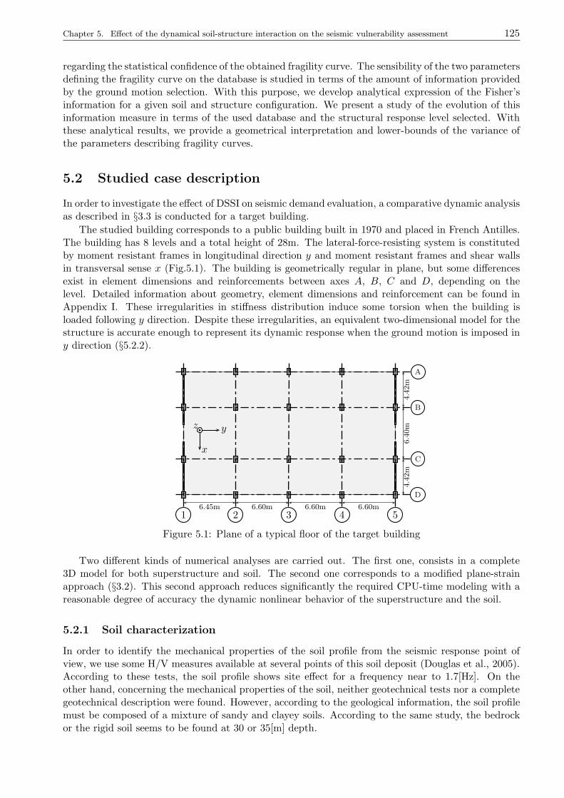
Chapter 5. Effect of the dynamical soil-structure interaction on the seismic vulnerability assessment 125
regarding the statistical confidence of the obtained fragility curve. The sensibility of the two parametersdefining the fragility curve on the database is studied in terms of the amount of information providedby the ground motion selection. With this purpose, we develop analytical expression of the Fisher’sinformation for a given soil and structure configuration. We present a study of the evolution of thisinformation measure in terms of the used database and the structural response level selected. Withthese analytical results, we provide a geometrical interpretation and lower-bounds of the variance ofthe parameters describing fragility curves.
5.2 Studied case description
In order to investigate the effect of DSSI on seismic demand evaluation, a comparative dynamic analysisas described in §3.3 is conducted for a target building.
The studied building corresponds to a public building built in 1970 and placed in French Antilles.The building has 8 levels and a total height of 28m. The lateral-force-resisting system is constitutedby moment resistant frames in longitudinal direction y and moment resistant frames and shear wallsin transversal sense x (Fig.5.1). The building is geometrically regular in plane, but some differencesexist in element dimensions and reinforcements between axes A, B, C and D, depending on thelevel. Detailed information about geometry, element dimensions and reinforcement can be found inAppendix I. These irregularities in stiffness distribution induce some torsion when the building isloaded following y direction. Despite these irregularities, an equivalent two-dimensional model for thestructure is accurate enough to represent its dynamic response when the ground motion is imposed iny direction (§5.2.2).
y
x
bz
1 2 3 4 56.45m 6.60m 6.60m 6.60m
D
C
B
A
4.4
2m
6.4
0m
4.4
2m
Figure 5.1: Plane of a typical floor of the target building
Two different kinds of numerical analyses are carried out. The first one, consists in a complete3D model for both superstructure and soil. The second one corresponds to a modified plane-strainapproach (§3.2). This second approach reduces significantly the required CPU-time modeling with areasonable degree of accuracy the dynamic nonlinear behavior of the superstructure and the soil.
5.2.1 Soil characterization
In order to identify the mechanical properties of the soil profile from the seismic response point ofview, we use some H/V measures available at several points of this soil deposit (Douglas et al., 2005).According to these tests, the soil profile shows site effect for a frequency near to 1.7[Hz]. On theother hand, concerning the mechanical properties of the soil, neither geotechnical tests nor a completegeotechnical description were found. However, according to the geological information, the soil profilemust be composed of a mixture of sandy and clayey soils. According to the same study, the bedrockor the rigid soil seems to be found at 30 or 35[m] depth.
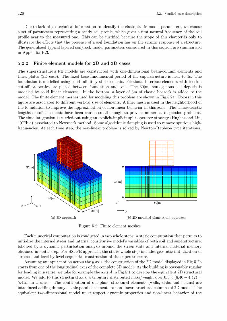
126 5.2. Studied case description
Due to lack of geotechnical information to identify the elastoplastic model parameters, we choosea set of parameters representing a sandy soil profile, which gives a first natural frequency of the soilprofile near to the measured one. This can be justified because the scope of this chapter is only toillustrate the effects that the presence of a soil foundation has on the seismic response of a structure.The generalized typical layered soil/rock model parameters considered in this section are summarizedin Appendix H.3.
5.2.2 Finite element models for 2D and 3D cases
The superstructure’s FE models are constructed with one-dimensional beam-column elements andthick plates (3D case). The fixed base fundamental period of the superstructure is near to 1s. Thefoundation is modelled using solid infinitely stiff elements. Frictional interface elements with tensioncut-off properties are placed between foundation and soil. The 30[m] homogenous soil deposit ismodeled by solid linear elements. In the bottom, a layer of 5m of elastic bedrock is added to themodel. The finite element meshes used for modeling this problem are shown in Fig.5.2a. Colors in thisfigure are associated to different vertical size of elements. A finer mesh is used in the neighborhood ofthe foundation to improve the approximation of non-linear behavior in this zone. The characteristiclengths of solid elements have been chosen small enough to prevent numerical dispersion problems.The time integration is carried-out using an explicit-implicit split operator strategy (Hughes and Liu,1977b,a) associated to Newmark method. Some algorithmic damping is used to remove spurious high-frequencies. At each time step, the non-linear problem is solved by Newton-Raphson type iterations.
yx
z80[m]
35[m]
30[m]
(a) 3D approach
35[m]
80[m]
y
z
(b) 2D modified plane-strain approach
Figure 5.2: Finite element meshes
Each numerical computation is conducted in two whole steps: a static computation that permits toinitialize the internal stress and internal constitutive model’s variables of both soil and superstructure,followed by a dynamic perturbation analysis around the stress state and internal material memoryobtained in static step. For SSI-FE approach, the static whole step includes geostatic initialization ofstresses and level-by-level sequential construction of the superstructure.
Assuming an input motion across the y axis, the construction of the 2D model displayed in Fig.5.2bstarts from one of the longitudinal axes of the complete 3D model. As the building is reasonably regularfor loading in y sense, we take for example the axis A in Fig.5.1 to develop the equivalent 2D structuralmodel. We add to this structural axis, a tributary distributed mass/weight over 0.5× (6.40 + 4.42) =5.41m in x sense. The contribution of out-plane structural elements (walls, slabs and beams) areintroduced adding dummy elastic parallel elements to non-linear structural columns of 2D model. Theequivalent two-dimensional model must respect dynamic properties and non-linear behavior of the
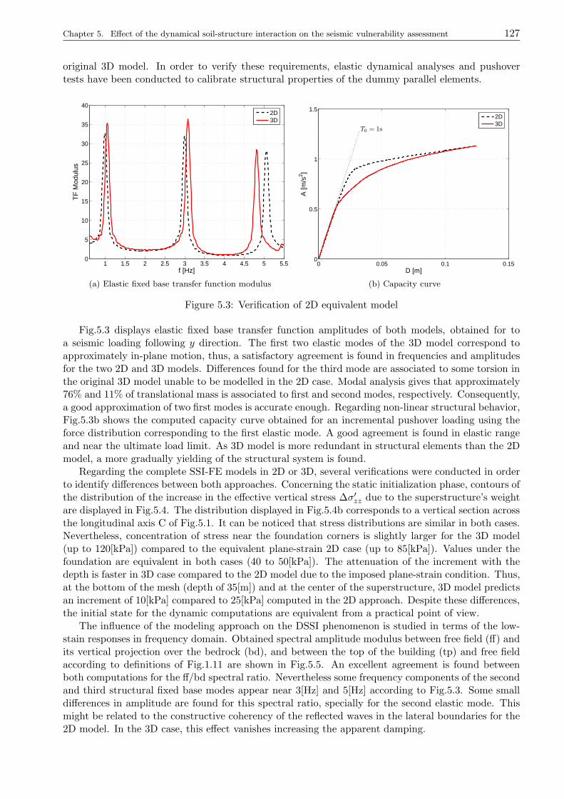
Chapter 5. Effect of the dynamical soil-structure interaction on the seismic vulnerability assessment 127
original 3D model. In order to verify these requirements, elastic dynamical analyses and pushovertests have been conducted to calibrate structural properties of the dummy parallel elements.
1 1.5 2 2.5 3 3.5 4 4.5 5 5.50
5
10
15
20
25
30
35
40
f [Hz]
TF
Mod
ulus
2D3D
(a) Elastic fixed base transfer function modulus
0 0.05 0.1 0.150
0.5
1
1.5
T0 = 1s
D [m]
A [m
/s2 ]
2D3D
(b) Capacity curve
Figure 5.3: Verification of 2D equivalent model
Fig.5.3 displays elastic fixed base transfer function amplitudes of both models, obtained for toa seismic loading following y direction. The first two elastic modes of the 3D model correspond toapproximately in-plane motion, thus, a satisfactory agreement is found in frequencies and amplitudesfor the two 2D and 3D models. Differences found for the third mode are associated to some torsion inthe original 3D model unable to be modelled in the 2D case. Modal analysis gives that approximately76% and 11% of translational mass is associated to first and second modes, respectively. Consequently,a good approximation of two first modes is accurate enough. Regarding non-linear structural behavior,Fig.5.3b shows the computed capacity curve obtained for an incremental pushover loading using theforce distribution corresponding to the first elastic mode. A good agreement is found in elastic rangeand near the ultimate load limit. As 3D model is more redundant in structural elements than the 2Dmodel, a more gradually yielding of the structural system is found.
Regarding the complete SSI-FE models in 2D or 3D, several verifications were conducted in orderto identify differences between both approaches. Concerning the static initialization phase, contours ofthe distribution of the increase in the effective vertical stress ∆σ′zz due to the superstructure’s weightare displayed in Fig.5.4. The distribution displayed in Fig.5.4b corresponds to a vertical section acrossthe longitudinal axis C of Fig.5.1. It can be noticed that stress distributions are similar in both cases.Nevertheless, concentration of stress near the foundation corners is slightly larger for the 3D model(up to 120[kPa]) compared to the equivalent plane-strain 2D case (up to 85[kPa]). Values under thefoundation are equivalent in both cases (40 to 50[kPa]). The attenuation of the increment with thedepth is faster in 3D case compared to the 2D model due to the imposed plane-strain condition. Thus,at the bottom of the mesh (depth of 35[m]) and at the center of the superstructure, 3D model predictsan increment of 10[kPa] compared to 25[kPa] computed in the 2D approach. Despite these differences,the initial state for the dynamic computations are equivalent from a practical point of view.
The influence of the modeling approach on the DSSI phenomenon is studied in terms of the low-stain responses in frequency domain. Obtained spectral amplitude modulus between free field (ff) andits vertical projection over the bedrock (bd), and between the top of the building (tp) and free fieldaccording to definitions of Fig.1.11 are shown in Fig.5.5. An excellent agreement is found betweenboth computations for the ff/bd spectral ratio. Nevertheless some frequency components of the secondand third structural fixed base modes appear near 3[Hz] and 5[Hz] according to Fig.5.3. Some smalldifferences in amplitude are found for this spectral ratio, specially for the second elastic mode. Thismight be related to the constructive coherency of the reflected waves in the lateral boundaries for the2D model. In the 3D case, this effect vanishes increasing the apparent damping.
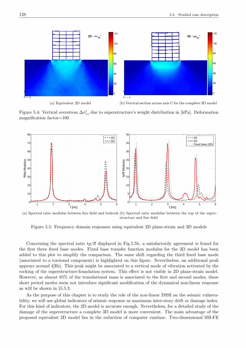
128 5.2. Studied case description
(a) Equivalent 2D model (b) Vertical section across axis C for the complete 3D model
Figure 5.4: Vertical overstress ∆σ′zz due to superstructure’s weight distribution in [kPa]. Deformationmagnification factor=100
1 2 3 4 5 60
10
20
30
40
50
60
70
80
f [Hz]
ff/bd
Mod
ulus
2D3D
(a) Spectral ratio modulus between free field and bedrock
1 2 3 4 5 60
5
10
15
20
25
30
35
40
f [Hz]
tp/ff
Mod
ulus
2D3DFixed base (3D)
(b) Spectral ratio modulus between the top of the super-structure and free field
Figure 5.5: Frequency domain responses using equivalent 2D plane-strain and 3D models
Concerning the spectral ratio tp/ff displayed in Fig.5.5b, a satisfactorily agreement is found forthe first three fixed base modes. Fixed base transfer function modulus for the 3D model has beenadded to this plot to simplify the comparison. The same shift regarding the third fixed base mode(associated to a torsional component) is highlighted on this figure. Nevertheless, an additional peakappears around 4[Hz]. This peak might be associated to a vertical mode of vibration activated by therocking of the superstructure-foundation system. This effect is not visible in 2D plane-strain model.However, as almost 85% of the translational mass is associated to the first and second modes, theseshort period modes seem not introduce significant modification of the dynamical non-linear responseas will be shown in §5.5.3.
As the purpose of this chapter is to study the role of the non-linear DSSI on the seismic vulnera-bility, we will use global indicators of seismic response as maximum inter-story drift or damage index.For this kind of indicators, the 2D model is accurate enough. Nevertheless, for a detailed study of thedamage of the superstructure a complete 3D model is more convenient. The main advantage of theproposed equivalent 2D model lies in the reduction of computer runtime. Two-dimensional SSI-FE
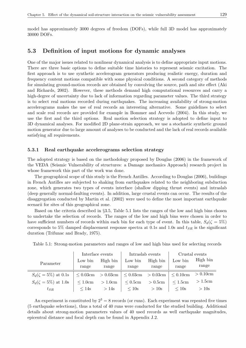
Chapter 5. Effect of the dynamical soil-structure interaction on the seismic vulnerability assessment 129
model has approximately 3000 degrees of freedom (DOFs), while full 3D model has approximately30000 DOFs.
5.3 Definition of input motions for dynamic analyses
One of the major issues related to nonlinear dynamical analysis is to define appropriate input motions.There are three basic options to define suitable time histories to represent seismic excitation. Thefirst approach is to use synthetic accelerogram generators producing realistic energy, duration andfrequency content motions compatible with some physical conditions. A second category of methodsfor simulating ground-motion records are obtained by convolving the source, path and site effect (Akiand Richards, 2002). However, these methods demand high computational resources and carry ahigh-degree of uncertainty due to lack of information regarding parameter values. The third strategyis to select real motions recorded during earthquakes. The increasing availability of strong-motionaccelerograms makes the use of real records an interesting alternative. Some guidelines to selectand scale real records are provided for example in Bommer and Acevedo (2004). In this study, weuse the first and the third options. Real motion selection strategy is adopted to define input to3D dynamical analyses. For modified 2D plane-strain approach, we use a stochastic synthetic groundmotion generator due to large amount of analyses to be conducted and the lack of real records availablesatisfying all requirements.
5.3.1 Real earthquake accelerograms selection strategy
The adopted strategy is based on the methodology proposed by Douglas (2006) in the framework ofthe VEDA (Seismic Vulnerability of structures: a Damage mechanics Approach) research project inwhose framework this part of the work was done.
The geographical scope of this study is the French Antilles. According to Douglas (2006), buildingsin French Antilles are subjected to shaking from earthquakes related to the neighboring subductionzone, which generates two types of events interface (shallow dipping thrust events) and intraslab(deep generally normal-faulting events). In addition, large crustal events can occur. The results of thedisaggregation conducted by Martin et al. (2002) were used to define the most important earthquakescenarii for sites of this geographical zone.
Based on the criteria described in §3.5, Table 5.1 lists the ranges of the low and high bins chosento undertake the selection of records. The ranges of the low and high bins were chosen in order tohave sufficient numbers of records within each bin for each type of event. In this table, Sd(ζ = 5%)corresponds to 5% damped displacement response spectra at 0.1s and 1.0s and tSR is the significantduration (Trifunac and Brady, 1975).
Table 5.1: Strong-motion parameters and ranges of low and high bins used for selecting records
Interface events Intraslab events Crustal events
ParameterLow binrange
High binrange
Low binrange
High binrange
Low binrange
High binrange
Sd(ζ = 5%) at 0.1s ≤ 0.03cm > 0.03cm ≤ 0.03cm > 0.03cm ≤ 0.10cm > 0.10cm
Sd(ζ = 5%) at 1.0s ≤ 1.0cm > 1.0cm ≤ 0.5cm > 0.5cm ≤ 1.5cm > 1.5cm
tSR ≤ 14s > 14s ≤ 10s > 10s ≤ 10s > 10s
An experiment is constituted by 23 = 8 records (or runs). Each experiment was repeated five times(5 earthquake selections), thus a total of 40 runs were conducted for the studied building. Additionaldetails about strong-motion parameters values of 40 used records as well earthquake magnitudes,epicentral distance and focal depth can be found in Appendix J.2.
130 5.3. Definition of input motions for dynamic analyses
5.3.2 Synthetic ground motion generation
There are many engineering methods for simulating ground motions. For example, procedures basedon random-vibration theory proposed by Saragoni and Hart (1974) or Nau et al. (1982) range fromfiltering and windowing Gaussian noise to generate accelerograms. As these methods are disconnectedfrom specific geophysical parameters, the resulting time histories are poorly correlated in terms ofearthquake scaling parameters. Other approaches generate seismic ground motion time histories thatare compatible with a prescribed response spectra (e.g. Gasparini and Vanmarcke, 1979; Deodatis,1996). The intrinsic problem of this kind of procedure is that in general the matching procedure maygenerate an excessive number of cycles of strong motion, producing an unrealistic high energy content.
In the present work, we adopt the empirical strategy developed by Pousse et al. (2006) that improvesthe stochastic model introduced by Sabetta and Pugliese (1996). In the method proposed by Sabettaand Pugliese (1996), the simulation of ground motion is achieved through an empirical method wheretime and frequency features of motion are derived from the signal spectogram PS(t, f) and depend onfew strong-motion indicators, such as Arias intensity (AI) (Arias, 1970) and the significant duration.According to Sabetta and Pugliese (1996), the spectogram can be factorized as,
PS(t, f) = PSτ (f)Pa(t) (5.1)
where PSτ (f) is the power spectral density function at time τ and Pa(t) is the instantaneous averagepower. In the original work of Sabetta and Pugliese (1996), PSτ (t) is represented by a collectionof power spectral densities described in terms of spectral moments. Pousse et al. (2006) propose toreplace this expression by the following function:
PSτ (f) =
(2πf)2
1+(
ffc
)2
maxS(f)√
1 +(
flog fc(τ)
)8e−Fc(τ) (5.2)
where S(f) is the Fourier spectra, fc is the corner frequency and Fc(τ) is the time evolution of thecentral frequency. The original lognormal shape for S(f) introduced by Sabetta and Pugliese (1996)was modified to a ω−square model to correct the deficit of energy in the low-frequency part of theFourier spectra. Additionally, Pousse et al. (2006) propose to model the instantaneous power as:
Pa(t) =1
25
AI
t√
2πσpe− 1
2σ2p(log t−µp)2
+24AI
25
1t√
2πσse− 1
2σ2s(log t−µs)2
t ≤ TcodaAt+T e
− 2πf(t+T )Qc t ≥ Tcoda
(5.3)
in order to take into account the arrival time, energy, and broadening of the P and S pulses withdistance, as well as the existence of scattered waves that produce the coda of the accelerogram. Inthe previous expression, µp, µs, σp and σs are the expected mean values and standard deviation of thedistribution of parameter t for the P and S pulses, respectively. The constant T and A are fixed bythe continuity condition of the function and its derivative at t = Tcoda. In equation (5.3), Qc is thefrequency dependent coda Q−value associated to coda decay.
Finally, the simulation of the ground motion is then performed summing Fourier series with time-dependent coefficients derived from PS(fn, t):
a(t) = 2N∑
n=1
√
2πf0 PS(fn, t) cos (n2πf0t+ φn) (5.4)
where a(t) is the acceleration, f0 is the fundamental frequency and φn the phases. In the originalSabetta and Pugliese (1996) model the difference among the simulated accelerograms was only due torandom phase φn. To better capture the variability of the observed ground motion, a Monte Carloexploration of the strong-motion indicators (e.g. tSR and AI), source parameters and envelope form(σs and Q(f)) was introduced to the model by Pousse et al. (2006).
Chapter 5. Effect of the dynamical soil-structure interaction on the seismic vulnerability assessment 131
In the original work of Sabetta and Pugliese (1996), the model was calibrated using predictiveequation from Italian strong-motion dataset. In the paper of Pousse et al. (2006), the model wascalibrated with Japanese data recorded by the K-net array. The generation tool used here correspondsto a calibration of the model conducted by the same authors, using the suitable west eurasia databasedescribed in Fukushima et al. (2003).
Due to lack of near-fault records in the west Eurasian database, Fukushima et al. (2003) adddata from other tectonic regions. However, added records are associated with the same earthquakecategory, i.e. shallow crustal earthquakes in active regions. According to Douglas (2006), suitablecrustal records for the French Antilles must be chosen conform to moment magnitude Mw between5.3 and 7.5 and focal depth inferior to 30km. As earthquake records included in the database usedto calibrate synthetic generator satisfy these criteria, obtained motions agrees with expected crustalmotions for French Antilles.
5.4 Analytical fragility curves
This section describes the adopted methodology to construct fragility curves on the basis of nonlineardynamic analysis. The procedure used here for establishing the fragility curves for seismic structuralresponse follows that proposed by Shinozuka et al. (2000). A strategy to estimate the amount of in-formation provided by an earthquake selection to construct fragility curves is developed and presentedin the following.
A Bernoulli experiment is a random experiment in which the outcome can be classified in one oftwo mutually exclusive ways: success or failure. If F (θ) denote the probability of success on each trialand Y the random variable itself, the probability density function (pdf) can be written as:
f(y, θ) = [F (θ)]y [1− F (θ)]1−y (5.5)
where y is a realization of the random variable Y and is equal to 1 for a success and equal to 0 fora failure. θ regroups the parameters describing F (θ). A sequence of Bernoulli trials occurs whena Bernoulli experiment is performed several independent times and that the probability of successremains the same from trial to trial. For a sample y1, y2, . . . yn of n values from Y , the multivariateprobability density associated with our observed data f (y1, . . . , yn; θ) as a function of θ with y1, . . . , ynfixed, is the likelihood function:
L(y; θ)
=N∏
k=1
[F (θ)]yk [1− F (θ)]1−yk (5.6)
F (·) can be interpreted as the probability of exceeding a specific value d of a response (usuallydamage) for a given earthquake severity ak, thus the fragility curve F (d|ak; θ). Consequently, yk = 1or 0 depending on whether or not the structure sustains the state d for an earthquake severity ak.Under the log-normal assumption of Shinozuka et al. (2000), F (·) takes the analytical form:
F (d|ak;α, β) = Φ
[1
βln( akα a
)]
= F (ak) (5.7)
in which Φ[·] is the standardized normal distribution function. α and β are two parameters describingthe fragility curve. We introduce here a normalization parameter a to obtain a non-dimensional valueof α, for example, the mean value of AIout of the considered ground motions.
The method of maximum likelihood estimates α and β by finding the values that maximizeL(y;α, β). Since maxima are unaffected by monotonous transformations, the problem is equivalent tomaximize:
lnL =n∑
k=1
[yk lnF (ak) + (1− yk) ln (1− F (ak))] (5.8)
132 5.4. Analytical fragility curves
hence, solving:
∂ lnL∂α
=∂ lnL∂β
= 0 (5.9)
Thus, after some algebra, the maximum condition can be expressed by:
n∑
k=1
Φ′(ak)αβ
[
− ykF (ak)
+1− yk
1− F (ak)
]
=
n∑
k=1
Iα(yk) = 0 (5.10)
n∑
k=1
Φ′(ak)β2
ln( akα a
)[
− ykF (ak)
+1− yk
1− F (ak)
]
=
n∑
k=1
Iβ(yk) = 0 (5.11)
The previous system of equations can be solved straightforwardly using standard optimizationalgorithms. The amount of information of Fisher provided by a n-sample about the set of parametersθ can be written as:
Ii,j(θ) = Cov
[∂ lnL∂θi
,∂ lnL∂θj
]
= E
[∂ lnL∂θi
.∂ lnL∂θj
]
− E[∂ lnL∂θi
]
E
[∂ lnL∂θj
]
(5.12)
where Ii,j is the general term of the symmetrical positive-definite Fisher information matrix, Cov[·]denotes the covariance and E[·] the expectation. This matrix corresponds to a measure of the abilityof the data to estimate the set of parameters α and β. Developing for the expectation value of thepartial derivative with respect to α:
E
[∂ lnL∂α
]
= E
[n∑
k=1
Iα(Yk)
]
=
∫
y1
. . .
∫
yn
n∑
k=1
Iα(yk) f(y1)dy1 . . . f(yn)dyn
=
∫
y1
Iαf(y1)dy1
∫
y2
. . .
∫
yn
f(y2)dy2 . . . f(yn)dyn
︸ ︷︷ ︸
=1
+ . . .
+
∫
yn
Iαf(yn)dyn
∫
y1
. . .
∫
yn−1
f(y1)dy1 . . . f(yn−1)dyn−1
︸ ︷︷ ︸
=1
= nE [Iα(Y )] (5.13)
Now, using the properties of the pdf f(y) and assuming that the sample size n is a large value, theexpectation can be approximated by the mean:
E [Iα(Y )] ≈ 1
n
n∑
k=1
Iα(yk;α, β) (5.14)
If the estimators α and β values of the fragility curve are used, right-hand term of the previousexpression is approximatively equal to zero. Similar analysis can be conducted for the expected value ofthe partial derivative with respect to β. Consequently, assuming a large number of sampling and usingmaximum likelihood estimators, the general term of the Fisher information matrix can be estimatedas:
Ii,j(θ) ≈ E[∂ lnL∂θi
.∂ lnL∂θj
]
(5.15)
Chapter 5. Effect of the dynamical soil-structure interaction on the seismic vulnerability assessment 133
Developing for example the cross parameter term Iα,β:
E
[∂ lnL∂α
.∂ lnL∂β
]
=
∫
y1
. . .
∫
yn
(n∑
k=1
Iα(yk)
)
.
(n∑
k=1
Iβ(yk)
)
f(y1)dy1 . . . f(yn)dyn
=
∫
y1
Iα(y1)Iβ(y1)f(y1)dy1
∫
y2
. . .
∫
yn
f(y2)dy2 . . . f(yn)dyn
︸ ︷︷ ︸
=1
+ . . .
+
∫
y1
Iα(y1)f(y1)dy1
∫
yn
Iβ(yn)dyn
∫
y2
. . .
∫
yn−1
f(y2)dy2 . . . f(yn−1)dyn−1
︸ ︷︷ ︸
=1
+ . . .
. . .+
∫
yn
Iα(yn)Iβ(yn)f(yn)dyn
∫
y2
. . .
∫
yn−1
f(y2)dy2 . . . f(yn−1)dyn−1
︸ ︷︷ ︸
=1
= nE [Iα(Y ) Iβ(Y )] +n!
(n− 2)!E [Iα(Y )] .E [Iβ(Y )] (5.16)
where ·! denotes the factorial. In a similar manner, assuming a large number of sampling and usingmaximum likelihood estimators, it is easy to probe that terms of estimators of Fisher informationmatrix can be computed as:
Iα,α =n∑
k=1
(Φ′(ak)
α β
)2 [
− ykF (ak)
+1− yk
1− F (ak)
]2
(5.17)
Iα,β =
n∑
k=1
(Φ′(ak))2
α β3lnakα a
[
− ykF (ak)
+1− yk
1− F (ak)
]2
(5.18)
Iβ,β =
n∑
k=1
(φ′(ak)
β2
)2 (
lnakα a
)2[
− ykF (ak)
+1− yk
1− F (ak)
]2
(5.19)
In order to obtain a bound of the variance associated to estimators of parameters, it is possible touse the Cramer-Rao inequality or the information inequality. For an estimator of a scalar parameter θ,the variance of any unbiased estimator θ of θ is lower-bounded by the inverse of the Fisher informationI(θ):
Var[
θ]
≥ 1
I(θ) (5.20)
where V [·] denotes the variance. For the multi-parameter case, if Θ denotes the estimator of a functionof the parameters θ and E[Θ] = ψ (θ), the Cramer-Rao bounds of the covariance matrix of Θ satisfies:
Cov [Θ] ≥∂ψ(θ)
∂θ[I(θ)]−1
(∂ψ(θ)
∂θ
)t
(5.21)
where the upperscript t denotes the transpose. If Θ is an unbiased estimator of θ, i.e. ψ(θ) = θ, thenthe Cramer-Rao bound reduces to:
Cov [θ] ≥ [I(θ)]−1 (5.22)
thus, the inverse of the Fisher information matrix provides the Cramer-Rao bounds, i.e. the relativecovariances of the simultaneous estimation of different parameters from a set of realizations. Undercertain weak regularity conditions, the maximum likelihood method is asymptotically optimal. Hence,the bias of the estimator tends to zero as the sample size increase to infinity. Additionally, the method
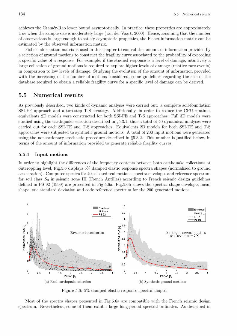
134 5.5. Numerical results
achieves the Cramer-Rao lower bound asymptotically. In practice, these properties are approximatelytrue when the sample size is moderately large (van der Vaart, 2000). Hence, assuming that the numberof observations is large enough to satisfy asymptotic properties, the Fisher information matrix can beestimated by the observed information matrix.
Fisher information matrix is used in this chapter to control the amount of information provided bya selection of ground motions to construct the fragility curve associated to the probability of exceedinga specific value of a response. For example, if the studied response is a level of damage, intuitively alarge collection of ground motions is required to explore higher levels of damage (relative rare events)in comparison to low levels of damage. Studying the evolution of the amount of information providedwith the increasing of the number of motions considered, some guidelines regarding the size of thedatabase required to obtain a reliable fragility curve for a specific level of damage can be derived.
5.5 Numerical results
As previously described, two kinds of dynamic analyses were carried out: a complete soil-foundationSSI-FE approach and a two-step T-S strategy. Additionally, in order to reduce the CPU-runtime,equivalents 2D models were constructed for both SSI-FE and T-S approaches. Full 3D models werestudied using the earthquake selection described in §5.3.1, thus a total of 40 dynamical analyses werecarried out for each SSI-FE and T-S approaches. Equivalents 2D models for both SSI-FE and T-Sapproaches were subjected to synthetic ground motions. A total of 200 input motions were generatedusing the nonstationary stochastic procedure described in §5.3.2. This number is justified below, interms of the amount of information provided to generate reliable fragility curves.
5.5.1 Input motions
In order to highlight the differences of the frequency contents between both earthquake collections atoutcropping level, Fig.5.6 displays 5% damped elastic response spectra shapes (normalized to groundacceleration). Computed spectra for 40 selected real motions, spectra envelopes and reference spectrumfor soil class S0 in seismic zone III (French Antilles) according to French seismic design guidelinesdefined in PS-92 (1999) are presented in Fig.5.6a. Fig.5.6b shows the spectral shape envelope, meanshape, one standard deviation and code reference spectrum for the 200 generated motions.
(a) Real earthquake selection (b) Synthetic ground motions
Figure 5.6: 5% damped elastic response spectra shapes.
Most of the spectra shapes presented in Fig.5.6a are compatible with the French seismic designspectrum. Nevertheless, some of them exhibit large long-period spectral ordinates. As described in
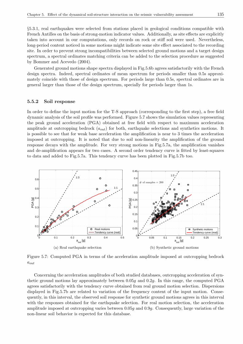
Chapter 5. Effect of the dynamical soil-structure interaction on the seismic vulnerability assessment 135
§5.3.1, real earthquakes were selected from stations placed in geological conditions compatible withFrench Antilles on the basis of strong-motion indicator values. Additionally, as site effects are explicitlytaken into account in our computations, only records on rock or stiff soil were used. Nevertheless,long-period content noticed in some motions might indicate some site effect associated to the recordingsite. In order to prevent strong incompatibilities between selected ground motions and a target designspectrum, a spectral ordinates matching criteria can be added to the selection procedure as suggestedby Bommer and Acevedo (2004).
Generated ground motions shape spectra displayed in Fig.5.6b agrees satisfactorily with the Frenchdesign spectra. Indeed, spectral ordinates of mean spectrum for periods smaller than 0.5s approxi-mately coincide with those of design spectrum. For periods large than 0.5s, spectral ordinates are ingeneral larger than those of the design spectrum, specially for periods larger than 1s.
5.5.2 Soil response
In order to define the input motion for the T-S approach (corresponding to the first step), a free fielddynamic analysis of the soil profile was performed. Figure 5.7 shows the simulation values representingthe peak ground acceleration (PGA) obtained at free field with respect to maximum accelerationamplitude at outcropping bedrock (aout) for both, earthquake selections and synthetics motions. Itis possible to see that for weak base acceleration the amplification is near to 3 times the accelerationimposed at outcropping. It is noted that due to soil non-linearity the amplification of the groundresponse decays with the amplitude. For very strong motions in Fig.5.7a, the amplification vanishesand de-amplification appears for two cases. A second order tendency curve is fitted by least-squaresto data and added to Fig.5.7a. This tendency curve has been plotted in Fig.5.7b too.
0 0.1 0.2 0.3 0.4 0.50
0.1
0.2
0.3
0.4
0.5
0.6
1:1
1:3
aout
[g]
PG
A [g
]
Real motionsTendency curve (real)
(a) Real earthquake selection
0 0.05 0.1 0.15 0.2 0.25 0.30
0.05
0.1
0.15
0.2
0.25
0.3
0.35
0.4
0.45
# of samples = 200
1:1
1:3
aout
[g]
PG
A [g
]
Synthetic motionsTendency curve (real)
(b) Synthetic ground motions
Figure 5.7: Computed PGA in terms of the acceleration amplitude imposed at outcropping bedrockaout
Concerning the acceleration amplitudes of both studied databases, outcropping acceleration of syn-thetic ground motions lay approximately between 0.05g and 0.2g. In this range, the computed PGAagrees satisfactorily with the tendency curve obtained from real ground motion selection. Dispersionsdisplayed in Fig.5.7b are related to variation of the frequency content of the input motion. Conse-quently, in this interval, the observed soil response for synthetic ground motions agrees in this intervalwith the responses obtained for the earthquake selection. For real motion selection, the accelerationamplitude imposed at outcropping varies between 0.05g and 0.9g. Consequently, large variation of thenon-linear soil behavior is expected for this database.
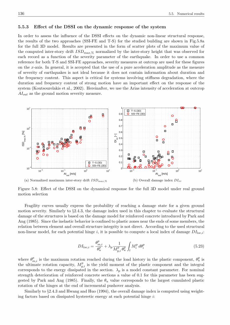
136 5.5. Numerical results
5.5.3 Effect of the DSSI on the dynamic response of the system
In order to assess the influence of the DSSI effects on the dynamic non-linear structural response,the results of the two approaches (SSI-FE and T-S) for the studied building are shown in Fig.5.8afor the full 3D model. Results are presented in the form of scatter plots of the maximum value ofthe computed inter-story drift ISDmax,% normalized by the inter-story height that was observed foreach record as a function of the severity parameter of the earthquake. In order to use a commonreference for both T-S and SSI-FE approaches, severity measures at outcrop are used for these figureson the x-axis. In general, it is accepted that the use of a pure acceleration amplitude as the measureof severity of earthquakes is not ideal because it does not contain information about duration andthe frequency content. This aspect is critical for systems involving stiffness degradation, where theduration and frequency content of strong motion have an important effect on the response of thesystem (Koutsourelakis et al., 2002). Hereinafter, we use the Arias intensity of acceleration at outcropAIout as the ground motion severity measure.
10−2
10−1
100
101
10−2
10−1
100
101
AIout
[m/s]
ISD
max
,% [%
]
T−S (3D)SSI−FE (3D)
(a) Normalized maximum inter-story drift ISDmax,%
10−2
10−1
100
101
0
0.1
0.2
0.3
0.4
0.5
0.6
0.7
0.8
0.9
1
AIout
[m/s]
DI ov
[−]
T−S (3D)SSI−FE (3D)
(b) Overall damage index DIov
Figure 5.8: Effect of the DSSI on the dynamical response for the full 3D model under real groundmotion selection
Fragility curves usually express the probability of reaching a damage state for a given groundmotion severity. Similarly to §2.4.3, the damage index used in this chapter to evaluate the structuraldamage of the structures is based on the damage model for reinforced concrete introduced by Park andAng (1985). Since the inelastic behavior is confined to plastic zones near the ends of some members, therelation between element and overall structure integrity is not direct. According to the used structuralnon-linear model, for each potential hinge i, it is possible to compute a local index of damage DIloc,i:
DIloc,i =θpm,iθpu
+ λp1
Mpy,i θ
pu
∫
t
Mpi dθ
pi (5.23)
where θpm,i is the maximum rotation reached during the load history in the plastic component, θpu isthe ultimate rotation capacity, Mp
y,i is the yield moment of the plastic component and the integralcorresponds to the energy dissipated in the section. λp is a model constant parameter. For nominalstrength deterioration of reinforced concrete sections a value of 0.1 for this parameter has been sug-gested by Park and Ang (1985). Finally, the θu value corresponds to the largest cumulated plasticrotation of the hinges at the end of incremental pushover analysis.
Similarly to §2.4.3 and Hwang and Huo (1994), the overall damage index is computed using weight-ing factors based on dissipated hysteretic energy at each potential hinge i:
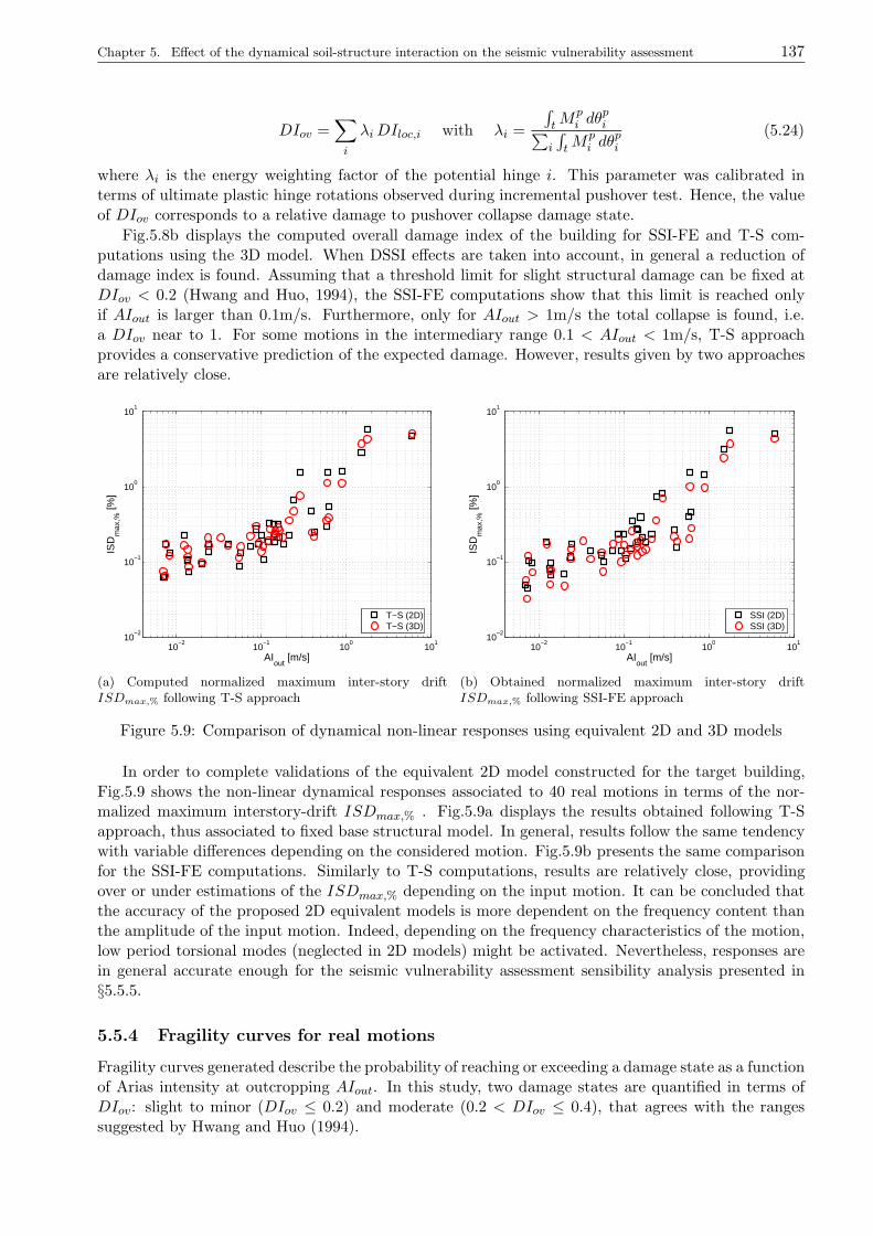
Chapter 5. Effect of the dynamical soil-structure interaction on the seismic vulnerability assessment 137
DIov =∑
i
λiDIloc,i with λi =
∫
tMpi dθ
pi
∑
i
∫
tMpi dθ
pi
(5.24)
where λi is the energy weighting factor of the potential hinge i. This parameter was calibrated interms of ultimate plastic hinge rotations observed during incremental pushover test. Hence, the valueof DIov corresponds to a relative damage to pushover collapse damage state.
Fig.5.8b displays the computed overall damage index of the building for SSI-FE and T-S com-putations using the 3D model. When DSSI effects are taken into account, in general a reduction ofdamage index is found. Assuming that a threshold limit for slight structural damage can be fixed atDIov < 0.2 (Hwang and Huo, 1994), the SSI-FE computations show that this limit is reached onlyif AIout is larger than 0.1m/s. Furthermore, only for AIout > 1m/s the total collapse is found, i.e.a DIov near to 1. For some motions in the intermediary range 0.1 < AIout < 1m/s, T-S approachprovides a conservative prediction of the expected damage. However, results given by two approachesare relatively close.
10−2
10−1
100
101
10−2
10−1
100
101
AIout
[m/s]
ISD
max
,% [%
]
T−S (2D)T−S (3D)
(a) Computed normalized maximum inter-story driftISDmax,% following T-S approach
10−2
10−1
100
101
10−2
10−1
100
101
AIout
[m/s]
ISD
max
,% [%
]
SSI (2D)SSI (3D)
(b) Obtained normalized maximum inter-story driftISDmax,% following SSI-FE approach
Figure 5.9: Comparison of dynamical non-linear responses using equivalent 2D and 3D models
In order to complete validations of the equivalent 2D model constructed for the target building,Fig.5.9 shows the non-linear dynamical responses associated to 40 real motions in terms of the nor-malized maximum interstory-drift ISDmax,% . Fig.5.9a displays the results obtained following T-Sapproach, thus associated to fixed base structural model. In general, results follow the same tendencywith variable differences depending on the considered motion. Fig.5.9b presents the same comparisonfor the SSI-FE computations. Similarly to T-S computations, results are relatively close, providingover or under estimations of the ISDmax,% depending on the input motion. It can be concluded thatthe accuracy of the proposed 2D equivalent models is more dependent on the frequency content thanthe amplitude of the input motion. Indeed, depending on the frequency characteristics of the motion,low period torsional modes (neglected in 2D models) might be activated. Nevertheless, responses arein general accurate enough for the seismic vulnerability assessment sensibility analysis presented in§5.5.5.
5.5.4 Fragility curves for real motions
Fragility curves generated describe the probability of reaching or exceeding a damage state as a functionof Arias intensity at outcropping AIout. In this study, two damage states are quantified in terms ofDIov: slight to minor (DIov ≤ 0.2) and moderate (0.2 < DIov ≤ 0.4), that agrees with the rangessuggested by Hwang and Huo (1994).
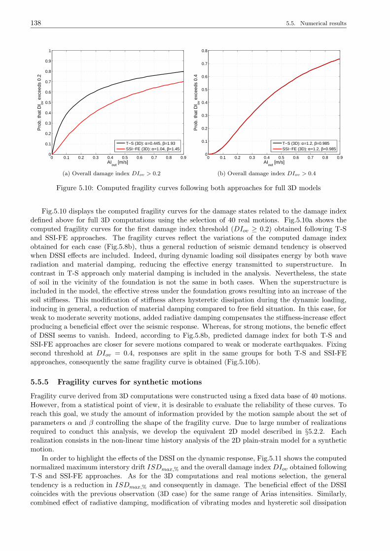
138 5.5. Numerical results
0 0.1 0.2 0.3 0.4 0.5 0.6 0.7 0.8 0.90
0.1
0.2
0.3
0.4
0.5
0.6
0.7
0.8
0.9
1
AIout
[m/s]
Pro
b. th
at D
I ov e
xcee
ds 0
.2
T−S (3D): α=0.445, β=1.93SSI−FE (3D): α=1.04, β=1.45
(a) Overall damage index DIov > 0.2
0 0.1 0.2 0.3 0.4 0.5 0.6 0.7 0.8 0.90
0.1
0.2
0.3
0.4
0.5
0.6
0.7
0.8
AIout
[m/s]
Pro
b. th
at D
I ov e
xcee
ds 0
.4
T−S (3D): α=1.2, β=0.985SSI−FE (3D): α=1.2, β=0.985
(b) Overall damage index DIov > 0.4
Figure 5.10: Computed fragility curves following both approaches for full 3D models
Fig.5.10 displays the computed fragility curves for the damage states related to the damage indexdefined above for full 3D computations using the selection of 40 real motions. Fig.5.10a shows thecomputed fragility curves for the first damage index threshold (DIov ≥ 0.2) obtained following T-Sand SSI-FE approaches. The fragility curves reflect the variations of the computed damage indexobtained for each case (Fig.5.8b), thus a general reduction of seismic demand tendency is observedwhen DSSI effects are included. Indeed, during dynamic loading soil dissipates energy by both waveradiation and material damping, reducing the effective energy transmitted to superstructure. Incontrast in T-S approach only material damping is included in the analysis. Nevertheless, the stateof soil in the vicinity of the foundation is not the same in both cases. When the superstructure isincluded in the model, the effective stress under the foundation grows resulting into an increase of thesoil stiffness. This modification of stiffness alters hysteretic dissipation during the dynamic loading,inducing in general, a reduction of material damping compared to free field situation. In this case, forweak to moderate severity motions, added radiative damping compensates the stiffness-increase effectproducing a beneficial effect over the seismic response. Whereas, for strong motions, the benefic effectof DSSI seems to vanish. Indeed, according to Fig.5.8b, predicted damage index for both T-S andSSI-FE approaches are closer for severe motions compared to weak or moderate earthquakes. Fixingsecond threshold at DIov = 0.4, responses are split in the same groups for both T-S and SSI-FEapproaches, consequently the same fragility curve is obtained (Fig.5.10b).
5.5.5 Fragility curves for synthetic motions
Fragility curve derived from 3D computations were constructed using a fixed data base of 40 motions.However, from a statistical point of view, it is desirable to evaluate the reliability of these curves. Toreach this goal, we study the amount of information provided by the motion sample about the set ofparameters α and β controlling the shape of the fragility curve. Due to large number of realizationsrequired to conduct this analysis, we develop the equivalent 2D model described in §5.2.2. Eachrealization consists in the non-linear time history analysis of the 2D plain-strain model for a syntheticmotion.
In order to highlight the effects of the DSSI on the dynamic response, Fig.5.11 shows the computednormalized maximum interstory drift ISDmax,% and the overall damage index DIov obtained followingT-S and SSI-FE approaches. As for the 3D computations and real motions selection, the generaltendency is a reduction in ISDmax,% and consequently in damage. The beneficial effect of the DSSIcoincides with the previous observation (3D case) for the same range of Arias intensities. Similarly,combined effect of radiative damping, modification of vibrating modes and hysteretic soil dissipation
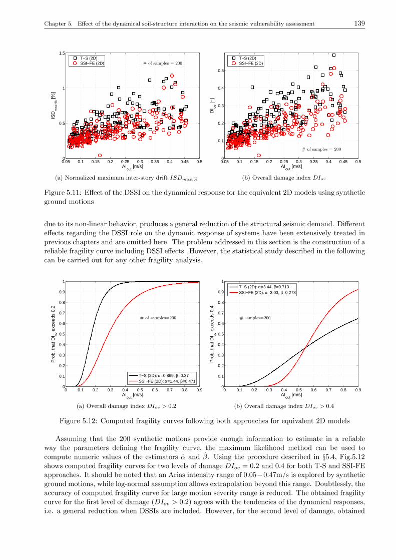
Chapter 5. Effect of the dynamical soil-structure interaction on the seismic vulnerability assessment 139
0.05 0.1 0.15 0.2 0.25 0.3 0.35 0.4 0.45 0.50
0.5
1
1.5
# of samples = 200
AIout
[m/s]
ISD
max
,% [%
]T−S (2D)SSI−FE (2D)
(a) Normalized maximum inter-story drift ISDmax,%
0.05 0.1 0.15 0.2 0.25 0.3 0.35 0.4 0.45 0.50
0.1
0.2
0.3
0.4
0.5
# of samples = 200
AIout
[m/s]
DI ov
[−]
T−S (2D)SSI−FE (2D)
(b) Overall damage index DIov
Figure 5.11: Effect of the DSSI on the dynamical response for the equivalent 2D models using syntheticground motions
due to its non-linear behavior, produces a general reduction of the structural seismic demand. Differenteffects regarding the DSSI role on the dynamic response of systems have been extensively treated inprevious chapters and are omitted here. The problem addressed in this section is the construction of areliable fragility curve including DSSI effects. However, the statistical study described in the followingcan be carried out for any other fragility analysis.
0 0.1 0.2 0.3 0.4 0.5 0.6 0.7 0.8 0.90
0.1
0.2
0.3
0.4
0.5
0.6
0.7
0.8
0.9
1
AIout
[m/s]
Pro
b. th
at D
I ov e
xcee
ds 0
.2
# of samples=200
T−S (2D): α=0.869, β=0.37SSI−FE (2D): α=1.44, β=0.471
(a) Overall damage index DIov > 0.2
0 0.1 0.2 0.3 0.4 0.5 0.6 0.7 0.8 0.90
0.1
0.2
0.3
0.4
0.5
0.6
0.7
0.8
0.9
1
AIout
[m/s]
Pro
b. th
at D
I ov e
xcee
ds 0
.4
# samples=200
T−S (2D): α=3.44, β=0.713SSI−FE (2D): α=3.03, β=0.278
(b) Overall damage index DIov > 0.4
Figure 5.12: Computed fragility curves following both approaches for equivalent 2D models
Assuming that the 200 synthetic motions provide enough information to estimate in a reliableway the parameters defining the fragility curve, the maximum likelihood method can be used tocompute numeric values of the estimators α and β. Using the procedure described in §5.4, Fig.5.12shows computed fragility curves for two levels of damage DIov = 0.2 and 0.4 for both T-S and SSI-FEapproaches. It should be noted that an Arias intensity range of 0.05−0.47m/s is explored by syntheticground motions, while log-normal assumption allows extrapolation beyond this range. Doubtlessly, theaccuracy of computed fragility curve for large motion severity range is reduced. The obtained fragilitycurve for the first level of damage (DIov > 0.2) agrees with the tendencies of the dynamical responses,i.e. a general reduction when DSSIs are included. However, for the second level of damage, obtained
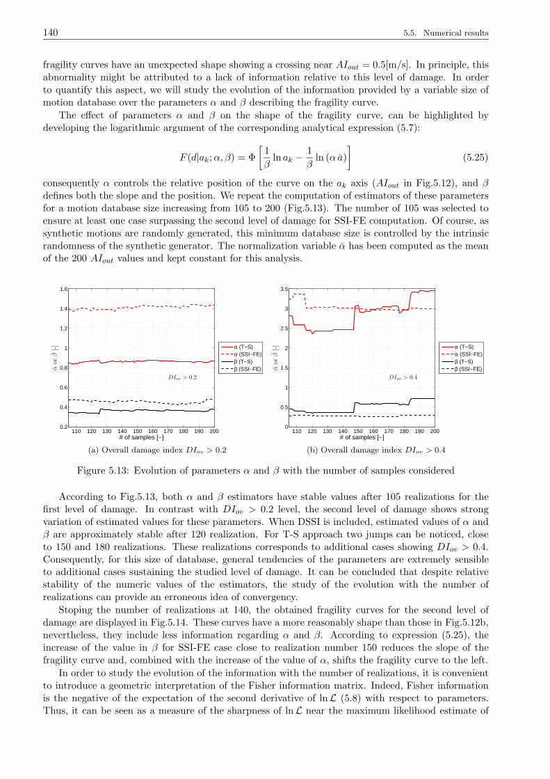
140 5.5. Numerical results
fragility curves have an unexpected shape showing a crossing near AIout = 0.5[m/s]. In principle, thisabnormality might be attributed to a lack of information relative to this level of damage. In orderto quantify this aspect, we will study the evolution of the information provided by a variable size ofmotion database over the parameters α and β describing the fragility curve.
The effect of parameters α and β on the shape of the fragility curve, can be highlighted bydeveloping the logarithmic argument of the corresponding analytical expression (5.7):
F (d|ak;α, β) = Φ
[1
βln ak −
1
βln (α a)
]
(5.25)
consequently α controls the relative position of the curve on the ak axis (AIout in Fig.5.12), and βdefines both the slope and the position. We repeat the computation of estimators of these parametersfor a motion database size increasing from 105 to 200 (Fig.5.13). The number of 105 was selected toensure at least one case surpassing the second level of damage for SSI-FE computation. Of course, assynthetic motions are randomly generated, this minimum database size is controlled by the intrinsicrandomness of the synthetic generator. The normalization variable α has been computed as the meanof the 200 AIout values and kept constant for this analysis.
110 120 130 140 150 160 170 180 190 2000.2
0.4
0.6
0.8
1
1.2
1.4
1.6
DIov > 0.2
αorβ
[-]
# of samples [−]
α (T−S)α (SSI−FE)β (T−S)β (SSI−FE)
(a) Overall damage index DIov > 0.2
110 120 130 140 150 160 170 180 190 2000
0.5
1
1.5
2
2.5
3
3.5
DIov > 0.4
αorβ
[-]
# of samples [−]
α (T−S)α (SSI−FE)β (T−S)β (SSI−FE)
(b) Overall damage index DIov > 0.4
Figure 5.13: Evolution of parameters α and β with the number of samples considered
According to Fig.5.13, both α and β estimators have stable values after 105 realizations for thefirst level of damage. In contrast with DIov > 0.2 level, the second level of damage shows strongvariation of estimated values for these parameters. When DSSI is included, estimated values of α andβ are approximately stable after 120 realization. For T-S approach two jumps can be noticed, closeto 150 and 180 realizations. These realizations corresponds to additional cases showing DIov > 0.4.Consequently, for this size of database, general tendencies of the parameters are extremely sensibleto additional cases sustaining the studied level of damage. It can be concluded that despite relativestability of the numeric values of the estimators, the study of the evolution with the number ofrealizations can provide an erroneous idea of convergency.
Stoping the number of realizations at 140, the obtained fragility curves for the second level ofdamage are displayed in Fig.5.14. These curves have a more reasonably shape than those in Fig.5.12b,nevertheless, they include less information regarding α and β. According to expression (5.25), theincrease of the value in β for SSI-FE case close to realization number 150 reduces the slope of thefragility curve and, combined with the increase of the value of α, shifts the fragility curve to the left.
In order to study the evolution of the information with the number of realizations, it is convenientto introduce a geometric interpretation of the Fisher information matrix. Indeed, Fisher informationis the negative of the expectation of the second derivative of lnL (5.8) with respect to parameters.Thus, it can be seen as a measure of the sharpness of lnL near the maximum likelihood estimate of
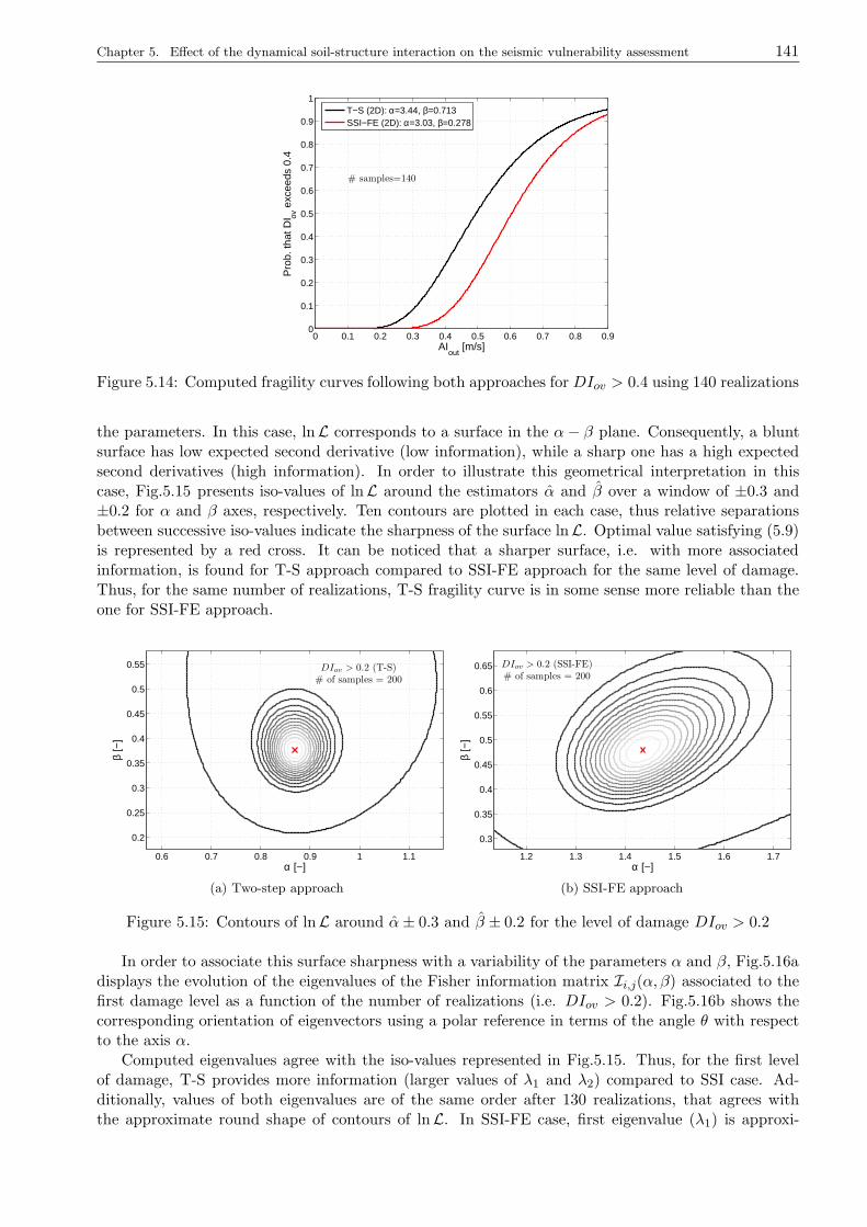
Chapter 5. Effect of the dynamical soil-structure interaction on the seismic vulnerability assessment 141
0 0.1 0.2 0.3 0.4 0.5 0.6 0.7 0.8 0.90
0.1
0.2
0.3
0.4
0.5
0.6
0.7
0.8
0.9
1
AIout
[m/s]
Pro
b. th
at D
I ov e
xcee
ds 0
.4
# samples=140
T−S (2D): α=3.44, β=0.713SSI−FE (2D): α=3.03, β=0.278
Figure 5.14: Computed fragility curves following both approaches for DIov > 0.4 using 140 realizations
the parameters. In this case, lnL corresponds to a surface in the α− β plane. Consequently, a bluntsurface has low expected second derivative (low information), while a sharp one has a high expectedsecond derivatives (high information). In order to illustrate this geometrical interpretation in thiscase, Fig.5.15 presents iso-values of lnL around the estimators α and β over a window of ±0.3 and±0.2 for α and β axes, respectively. Ten contours are plotted in each case, thus relative separationsbetween successive iso-values indicate the sharpness of the surface lnL. Optimal value satisfying (5.9)is represented by a red cross. It can be noticed that a sharper surface, i.e. with more associatedinformation, is found for T-S approach compared to SSI-FE approach for the same level of damage.Thus, for the same number of realizations, T-S fragility curve is in some sense more reliable than theone for SSI-FE approach.
DIov > 0.2 (T-S)# of samples = 200
α [−]
β [−
]
0.6 0.7 0.8 0.9 1 1.1
0.2
0.25
0.3
0.35
0.4
0.45
0.5
0.55
(a) Two-step approach
DIov > 0.2 (SSI-FE)# of samples = 200
α [−]
β [−
]
1.2 1.3 1.4 1.5 1.6 1.7
0.3
0.35
0.4
0.45
0.5
0.55
0.6
0.65
(b) SSI-FE approach
Figure 5.15: Contours of lnL around α± 0.3 and β ± 0.2 for the level of damage DIov > 0.2
In order to associate this surface sharpness with a variability of the parameters α and β, Fig.5.16adisplays the evolution of the eigenvalues of the Fisher information matrix Ii,j(α, β) associated to thefirst damage level as a function of the number of realizations (i.e. DIov > 0.2). Fig.5.16b shows thecorresponding orientation of eigenvectors using a polar reference in terms of the angle θ with respectto the axis α.
Computed eigenvalues agree with the iso-values represented in Fig.5.15. Thus, for the first levelof damage, T-S provides more information (larger values of λ1 and λ2) compared to SSI case. Ad-ditionally, values of both eigenvalues are of the same order after 130 realizations, that agrees withthe approximate round shape of contours of lnL. In SSI-FE case, first eigenvalue (λ1) is approxi-
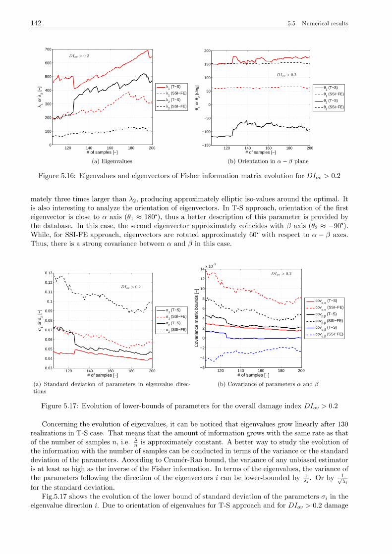
142 5.5. Numerical results
120 140 160 180 2000
100
200
300
400
500
600
700
DIov > 0.2
λ 1 or
λ 2 [−]
# of samples [−]
λ1 (T−S)
λ1 (SSI−FE)
λ2 (T−S)
λ2 (SSI−FE)
(a) Eigenvalues
120 140 160 180 200−150
−100
−50
0
50
100
150
200
DIov > 0.2
θ 1 or
θ 2 [deg
]
# of samples [−]
θ1 (T−S)
θ1 (SSI−FE)
θ2 (T−S)
θ2 (SSI−FE)
(b) Orientation in α− β plane
Figure 5.16: Eigenvalues and eigenvectors of Fisher information matrix evolution for DIov > 0.2
mately three times larger than λ2, producing approximately elliptic iso-values around the optimal. Itis also interesting to analyze the orientation of eigenvectors. In T-S approach, orientation of the firsteigenvector is close to α axis (θ1 ≈ 180°), thus a better description of this parameter is provided bythe database. In this case, the second eigenvector approximately coincides with β axis (θ2 ≈ −90°).While, for SSI-FE approach, eigenvectors are rotated approximately 60° with respect to α − β axes.Thus, there is a strong covariance between α and β in this case.
120 140 160 180 2000.03
0.04
0.05
0.06
0.07
0.08
0.09
0.1
0.11
0.12
0.13
DIov > 0.2
σ 1 or
σ 2 [−]
# of samples [−]
σ1 (T−S)
σ1 (SSI−FE)
σ2 (T−S)
σ2 (SSI−FE)
(a) Standard deviation of parameters in eigenvalue direc-tions
120 140 160 180 200−6
−4
−2
0
2
4
6
8
10
12
14x 10
−3
DIov > 0.2
Cov
aria
nce
mat
rix b
ound
s [−
]
# of samples [−]
covα,α (T−S)
covα,α (SSI−FE)
covβ,β (T−S)
covβ,β (SSI−FE)
covα,β (T−S)
covα,β (SSI−FE)
(b) Covariance of parameters α and β
Figure 5.17: Evolution of lower-bounds of parameters for the overall damage index DIov > 0.2
Concerning the evolution of eigenvalues, it can be noticed that eigenvalues grow linearly after 130realizations in T-S case. That means that the amount of information grows with the same rate as thatof the number of samples n, i.e. λ
nis approximately constant. A better way to study the evolution of
the information with the number of samples can be conducted in terms of the variance or the standarddeviation of the parameters. According to Cramer-Rao bound, the variance of any unbiased estimatoris at least as high as the inverse of the Fisher information. In terms of the eigenvalues, the variance ofthe parameters following the direction of the eigenvectors i can be lower-bounded by 1
λi. Or by 1√
λi
for the standard deviation.
Fig.5.17 shows the evolution of the lower bound of standard deviation of the parameters σi in theeigenvalue direction i. Due to orientation of eigenvalues for T-S approach and for DIov > 0.2 damage

Chapter 5. Effect of the dynamical soil-structure interaction on the seismic vulnerability assessment 143
level, the values of σ1 and σ2 can be interpreted directly as lower-bound of the standard deviation ofα and β, respectively. Thus, according to Fig.5.17a and Fig.5.12a, the value of α obtained with 200realizations is approximately equal to 0.86 with a standard deviation of at least 0.04, similarly, 0.37for β with a standard deviation of at least 0.045. Consequently, coefficients of variation of at least5% and 12%, for α and β respectively are obtained. This information might be used to constructconfidence intervals for α and β and define families of fragility curves by varying the confidence onthe parameters for example. However, the strategy described before gives a lower-bound of standarddeviation of parameters defining fragility curve. Consequently, the use of this information to estimateconfidence intervals requires judgement.
Due to the orientation of eigenvectors for SSI-FE approach, the analysis of the variance of theestimated parameters is conducted directly with the inverse of the Fisher information matrix accordingto expression (5.22). Thus, Fig.5.17b displays the evolution of the lower-bounds of the covariancematrix terms for both approaches associated to the first level of damage. It can be noticed thatthe cross term Covα,β is near to zero after 130 samples in T-S case, while it is negative and of thesame order as the diagonal terms for the SSI-FE approach. These curves confirm the evolution oforientations shown in Fig.5.16. Regarding the diagonal terms of the bound covariance matrix, largeuncertainty is associated to α parameter in comparison to β for SSI-FE case, that is the opposite ofT − S case. Additionally, variances in SSI-FE approach are significantly larger than those in the T-Sapproach. Consequently, larger uncertainties are associated to the position rather than to the slope ofthe fragility curve. These conclusions can not be derived directly from the evolution of α or β with thenumber of samples (Fig.5.13). Thus, it can be concluded that the apparent stabilization of estimatorsmust not to be interpreted as a convergency of the fragility curves. In this case, curves associated toSSI-FE are less reliable on a statistically point of view compared to those derived from T-S results.
DIov > 0.4 (T-S)# of samples = 200
α [−]
β [−
]
3.1 3.2 3.3 3.4 3.5 3.6 3.7 3.8
0.5
0.6
0.7
0.8
0.9
1
(a) Two-step approach
DIov > 0.4 (SSI-FE)# of samples = 200
α [−]
β [−
]
2.6 2.7 2.8 2.9 3 3.1 3.2 3.30
0.1
0.2
0.3
0.4
0.5
(b) SSI-FE approach
Figure 5.18: Contours of lnL around α± 0.4 and β ± 0.3 for the level of damage DIov > 0.4
Concerning the second level of damage (DIov > 0.4), Fig.5.18 shows the iso-values of lnL for 200realizations, around the optimal values of α and β for a window of ±0.4 and ±0.3 in α and β axes,respectively. Ten contours are plotted in each case, to make comparisons between both approachespossible. According to this figure, there are large uncertainties regarding one of the principal directions(large separation in iso-values). Fig.5.19 shows the corresponding eigenvectors and eigenvalues.
It can be noticed that the first eigenvalue (λ1) is very close to β axis in both cases (θ1 ≈ 80°).Consequently, second eigenvector corresponds approximately to α value. According to the numericalvalue of λ2, there is very few information regarding α, i.e. the relative position of the fragility curvein the AIout axis (Fig.5.12b). Additionally, according to the evolution of λ1 with the number ofsamples, information provided by the motions in T-S case is very erratic, while λ1 for SSI-FE growsmonotonically with the number of samples. Indeed, there is an abrupt broke near to 150 realizations

144 5.5. Numerical results
120 140 160 180 2000
50
100
150
200
250
300
DIov > 0.4
λ 1 or
λ 2 [−]
# of samples [−]
λ1 (T−S)
λ1 (SSI−FE)
λ2 (T−S)
λ2 (SSI−FE)
(a) Eigenvalues
120 140 160 180 20060
80
100
120
140
160
180
DIov > 0.4
θ 1 or
θ 2 [deg
]
# of samples [−]
θ1 (T−S)
θ1 (SSI−FE)
θ2 (T−S)
θ2 (SSI−FE)
(b) Orientation in α− β plane
Figure 5.19: Eigenvalues and eigenvectors of Fisher information matrix evolution for DIov > 0.4
in T-S case due to the apparition of realizations satisfying the damage criterion. Thus, for this level ofdamage, the database is not large enough and there is a great sensibility to additional cases sustainingthe studied level of damage. Even if evolution of λ1 for the SSI-FE analysis seems stabilized (λ1
n
approximately constant), the second eigenvalue λ2 is close to zero. Assuming that λ1 correspondsapproximately to the lower-bound of variance of β in SSI-FE case, for 200 realizations we obtain thatβ = 0.278 with a variance of at least 1√
λ1≈ 0.06, thus a coefficient of variation of 20%. For the
second parameter α, as λ2 is close to zero we have a very large lower-bound standard deviation. Inconclusion, there is not enough information to construct fragility curves for this level of damage. Onthe basis of these arguments, we need to increase significantly the number of realizations and/or toadd stronger records exploring a larger range of motion severity in order to increase data sustainingthe second level of damage.
Table 5.2: Eigenvalues and eigenvectors for real ground motion selection used for 3D models
T-S SSI-FE
Parameter DIov > 0.2 DIov > 0.4 DIov > 0.2 DIov > 0.4
λ1 66 21 50 33
θ1 −80° −60° −80° −70°λ2 5 3 6 4
θ2 −170° −150° −170° −160°To complete this analysis, it is interesting to estimate the information provided by real ground mo-
tion collection used to compute fragility curves for 3D models (§5.5.4). Rounded values of eigenvaluesand eigenvectors for T-S and SSI-FE approaches are summarized in Tab.5.2 for the 40 real motionsselected, and for the two levels of damages explored. According to eigenvector orientations, for allcombinations the first eigenvector is close to β axis (θ1 ≈ 80°) and the second eigenvector is close toα axis, i.e. associated to the position of the fragility curve. In general, eigenvalues are significantlysmaller than those obtained for the synthetic motion study. For example, for the first level of damageof T-S case, the lower bound of the standard deviation can be obtained as 1√
λ1≈ 0.12. According to
the value of β in Fig.5.10b, the corresponding coefficient of variation is at least of 33%. Performing thesame computation for the other parameters we obtain larger coefficients of variation. Consequently,this 40 real motions selection give a poor description in a statistically point of view of the parametersdescribing the fragility curve. This conclusion is not evident from the fragility curves, highlighting theimportance of the provided information analysis presented in this section.
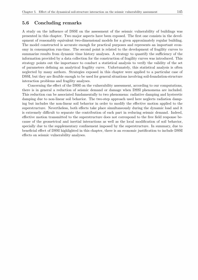
Chapter 5. Effect of the dynamical soil-structure interaction on the seismic vulnerability assessment 145
5.6 Concluding remarks
A study on the influence of DSSI on the assessment of the seismic vulnerability of buildings waspresented in this chapter. Two major aspects have been exposed. The first one consists in the devel-opment of reasonably equivalent two-dimensional models for a given approximately regular building.The model constructed is accurate enough for practical purposes and represents an important econ-omy in consumption run-time. The second point is related to the development of fragility curves tosummarize results from dynamic time history analyses. A strategy to quantify the sufficiency of theinformation provided by a data collection for the construction of fragility curves was introduced. Thisstrategy points out the importance to conduct a statistical analysis to verify the validity of the setof parameters defining an analytical fragility curve. Unfortunately, this statistical analysis is oftenneglected by many authors. Strategies exposed in this chapter were applied to a particular case ofDSSI, but they are flexible enough to be used for general situations involving soil-foundation-structureinteraction problems and fragility analyses.
Concerning the effect of the DSSI on the vulnerability assessment, according to our computations,there is in general a reduction of seismic demand or damage when DSSI phenomena are included.This reduction can be associated fundamentally to two phenomena: radiative damping and hystereticdamping due to non-linear soil behavior. The two-step approach used here neglects radiation damp-ing but includes the non-linear soil behavior in order to modify the effective motion applied to thesuperstructure. Nevertheless, both effects take place simultaneously during the dynamic load and itis extremely difficult to separate the contribution of each part in reducing seismic demand. Indeed,effective motion transmitted to the superstructure does not correspond to the free field response be-cause of the geometrical and inertial interactions as well as the local modification of soil behavior,specially due to the supplementary confinement imposed by the superstructure. In summary, due tobeneficial effect of DSSI highlighted in this chapter, there is an economic justification to include DSSIeffects on seismic vulnerability analyses.

146 5.6. Concluding remarks

Chapter 5. Effect of the dynamical soil-structure interaction on the seismic vulnerability assessment 147
————————————————————————————————-Conclusions

148 5.6. Concluding remarks
Conclusions
Summary
In the preceding chapters we have investigated various aspects of the dynamical non-linear SSI. Evenif this problem has been the subject of numerous investigations, no simple realistic solution exists forthe introduction of the non-linear soil behavior. The major goal of this thesis was to contribute to theunderstanding of the role of the non-linear soil behavior over the complete problem.
Chapter 1 provides theoretical basis for non-linear DSSI modeling using Finite Element Method.Special developments in the used FE code GEFDyn were done, in order to increase the performanceof the code and enhance its capabilities to model structural non-linear behavior. The major issuerelated to numerical modeling is the treatment of the lateral boundaries and damping. Modelingissues associated to the treatment of the lateral boundaries and damping were explored in the form ofseveral numerical validations, in order to justify different adopted choices.
In Chapter 2 we looked into the influence of DSSI effects on the seismic performance evaluation ofstructures. A parametric study concerning the structure, the input signal and the soil was conducted.The main conclusion of this chapter was that the soil-structure interaction with a non-linear soil modelcan vary significantly the response of the considered set of structures with respect to those with fixedbase condition. In terms of the Capacity Spectrum Method, this chapter points out that the majorchallenge to quantify the non-linear SSI effects in seismic demand evaluation is to predict an accurateglobal damping, able to be used in simpler approaches. Three important aspects of the problem weredetected: limitations associated to a 2D plane-strain approach, contribution of the elastic part of thesoil behavior to the DSSI and the influence of the seismic database on the obtained fragility curves.Each aspect was studied in detail in the other chapters of this document.
In Chapter 3, a modified formulation of standard plane-strain model suitable for regular buildingswas presented. The main advantage of the proposed approach lies in the CPU time consumptionreduction. The approach was validated and successfully applied to two buildings on three differentsoils. The effects of the non-linear DSSI result in a variation of the computed structural responsecompared to that obtained with fixed base condition, even if the non-linear behavior of the soil istaken into account to estimate the imposed free field motion. The evaluation of some energy dissipationmeasure has been done to highlight the influence of the initial state modification induced by the selfweight of the superstructure. Though the self weigh contributes to increase the stiffness of the soilbelow the foundation, this additional confinement reduces hysteretic behavior under dynamic loading,compensating strain field generated by the superstructure oscillations. In the case of liquefiable soil,severe motions inducing extensive pore pressure build-up result into approximately elastic structuralresponse. In these case, structure responds essentially as a rigid block compared to extensively stiffnessdegraded soil. Generalization of DSSI effects on displacement demand for a given building on a definedsoil was unsuccessful. Large dispersion of results can be associated to the complexity of several non-linear inter-dependant phenomena.
Chapter 4 describes the investigation conducted in order to define the contribution of the pureelastic DSSI effects in the complete non-linear DSSI problem. With this purpose, a comparative anal-ysis between elastic and inelastic soil behavior assumptions for two SDOF structures and two soils iscarried out. The results point out that, in general, inelastic soil behavior plays a decisive role onlywhen the soil is saturated. When the soil is in dry condition, an elastic DSSI approach seems to be
150 5.6. Concluding remarks
accurate enough to take into account the modification of the structural response due to DSSI. Differ-ences in structural dynamics responses are related to pore pressure generation induced in the inelasticcase and neglected when elastic soil behavior is assumed. The influence of interaction phenomenon forthe low-rise SDOF structure considered is quite erratic. Hence, depending on the characteristics of theground motion DSSI effects are beneficial or detrimental in dry soil case. In saturated case, inelasticDSSI effects are in general beneficial. Regarding the studied mid-rise superstructure, in both dryand saturated soil cases, the effects of the DSSI are favorable in reducing the expected displacementductility demand.
Finally, the Chapter 5, is devoted to the development of analytical fragility curves including DSSIeffects. Major attention is focused in the statistical confidence of the obtained fragility curve. Withthis purpose, a strategy to study the sensibility of the two parameters defining the fragility curveon the database in terms of the amount of information provided by the ground motion selection isdeveloped. A set of analytical expressions are derived in order to provide a geometrical interpretationof the parameters describing fragility curves. Strategies presented in this chapter were applied to aparticular case of DSSI, but they are flexible enough to be used for general situations involving seismicfragility analyses. The strategy presented points out the importance of conducting a statistical analysisto verify the validity of the set of parameters defining an analytical fragility curve.
Overall conclusions
According to the investigation conducted in this work, except for some cases described in Chapter4, there is in general a reduction of seismic demand or structural damage when non-linear DSSIphenomenon is included. This reduction can be associated fundamentally to two phenomena: radiativedamping and hysteretic damping due to non-linear soil behavior. The two-step approach used asreference throughout this work, neglects radiation damping but includes the non-linear soil behaviorin order to modify the effective motion applied to the superstructure. Nevertheless, both effects takeplace simultaneously during the dynamic load and it is extremely difficult to separate the contributionof each part in reducing seismic demand. Indeed, effective motion transmitted to the superstructuredoes not correspond to the free field response because of the geometrical and inertial interactions aswell as the local modification of soil behavior, specially due to the supplementary confinement imposedby the superstructure’s weight. Large efforts have been made in order to generalize findings with alimited success. A series of strong-motion severity measures, structural damage measures and energydissipation indicators have been introduced and studied for this purpose. Nevertheless, results are ingeneral erratic and consequently, generalization was extremely difficult.
The results of the work illustrate clearly the importance of accounting for the non-linear soilbehavior. In this case, the major part of non-linear DSSI effects are beneficial related to decreasingthe maximum seismic structural demand. However, the non-linear DSSI could increase or decrease theexpected structural damage depending on the type of the structure, the input motion, and the dynamicsoil properties. Furthermore, there is an economic justification to take into account the modificationeffects due to non-linear soil behavior. Further investigations in this direction are needed in order toobtain more general conclusions for diverse structure and soil typologies.
Further research
The current seismic design philosophy is based on non-linear behavior of structures. Thus, designbase shear provided by design codes are intentionally much lower than the lateral strength required toensure an elastic structural behavior. The ratio between the lateral yielding strength required to avoidinelastic behavior and the lateral yield required to sustain a ductility ratio demand µ is usually knownas strength reduction factor Rµ. During the last decades, several investigations have been conducted inorder to improve the reliability of the reduction factors in design provisions. Later, some investigationswere conducted in order to point out the effect of the soil conditions (e.g. Miranda and Vertero 1994).
Chapter 5. Effect of the dynamical soil-structure interaction on the seismic vulnerability assessment 151
More recent investigations on site-dependent strength reduction factors for soil-structure interactingsystems (Ciampoli and Pinto, 1995; Rodriguez and Montes, 2000; Ghannad and Jahankhah, 2007;Aviles and Perez-Rocha, 2003) have shown the effects of the DSSI. Nevertheless, these studies havebeen developed using standard approximations for linear elastic DSSI, thus, the effects of the non-linearDSSI has not been considered yet. Findings presented in this work have illustrated the importanceof accounting for the non-linear soil behavior. Consequently, the development of Rµ including non-linear site and non-linear DSSI effects can lead to a more reliable seismic design of structures. Theuse of the methodology presented in this work can contribute to a better understanding of the DSSIeffects on the seismic structural design. Of course, the development of this kind of relations needs anextensive parametric investigation on diverse soils, structures and foundations typologies. In addition,the modified plane-strain approach presented in this work might considerably contribute to reduce theCPU time required for such large parametric studies.
The assessment of building damage caused by ground motions requires the definition of building’scapacity and vulnerability as a function of the demand. In this problem, there are several sourcesof uncertainty: the earthquake (demand), the soil and the building itself. Only the problem of thedemand variability has been addressed in Chapter 5. Nevertheless in practice the properties of the soilvary as much, exhibiting strong inhomogeneities very difficult to estimate. The risk of damage in soil-structure systems including variability in both, soil and earthquake, has been studied for liquefiablesoils (Koutsourelakis et al., 2002; Popescu, 2002; Popescu et al., 2006). However, in these studies,structural damage is estimated using foundation responses (settlement or tilt). Indeed, in these studiesthe effect of the structural damage in the DSSI has been neglected assuming elastic structures. Thissimplification is satisfactory for liquefiable soils when structure responds essentially as a rigid block.However, for more general cases, the inelasticity of the superstructure must be included in the analysis.The vulnerability assessment strategy developed in this work can be extended straightforwardly totake into account soil variability. Indeed, the statistical confidence strategy presented in this work isstill valid for several sources of uncertainties. Consequently, this aspect could be easily studied.
Concerning the numerical modeling of the DSSI problem, this work was conducted using the so-called direct method. The substructure method in frequency domain was employed as a tool fornumerical validation in elastic case. Nevertheless, there are methods that combine advantages ofboth the direct and substructure method called hybrid method. Usually, a bounded soil domain(near-field) is treated with FEM, while the unbounded soil domain (far-field) is treated with BEM.When material non-linearities are taken into account in near-field, an iterative procedure is carriedout to compute interaction forces between both domains. Other sub-structuring methods as theDomain Reduction Method (Bielak et al., 2003) can be used. These kinds of techniques are compatiblewith the problem addressed in this work and might reduce some wave reflections detected whena tied lateral approach is used. Similarly, other possible improvements to our computations areassociated to absorbing boundary conditions. In this work, we use paraxial approximation to computetime domain impedances. This approximation is exact only for normal incident waves. Currently,better approximations for this problem exist (e.g. Berenger 1994; Basu and Chopra 2003). Therefore,some reduction of wave reflections could be obtained by implementing these absorbing boundaries inGEFDyn .
Finally, the main drawback of the adopted strategy is related to the large amount of parametersassociated to each FE model. The good performance of each model has been studied by numericalvalidations under elastic assumption. The calibration of the soil constitutive model parameter hasbeen carried out using reference laboratory test results when available. Nevertheless, no experimentalcalibrations of the complete non-linear FE models have been done. Doubtlessly, validations againstinstrumented sites or physical experiments performed in a shaking table or in a centrifuge in inelasticrange are desirable.

152 5.6. Concluding remarks

Appendices

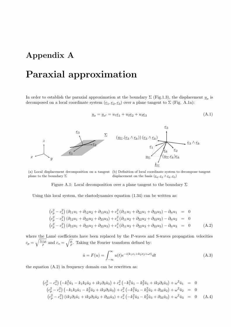
Appendix A
Paraxial approximation
In order to establish the paraxial approximation at the boundary Σ (Fig.1.3), the displacement us isdecomposed on a local coordinate system (e1, e2, e3) over a plane tangent to Σ (Fig. A.1a):
us = us′ = u1e1 + u2e2 + u3e3 (A.1)
x y
z
e1
e2
e3Σ
(a) Local displacement decomposition on a tangentplane to the boundary Σ
e1e2
e3
kΣ
ekuΣ (uΣ.ek)ek
e3 ∧ ek(uΣ.(e3 ∧ ek)) (e3 ∧ ek)
(b) Definition of local coordinate system to decompose tangentdisplacement on the basis (ek, e3 ∧ ek, e3)
Figure A.1: Local decomposition over a plane tangent to the boundary Σ
Using this local system, the elastodynamics equation (1.34) can be written as:
(c2p − c2s
)(∂11u1 + ∂12u2 + ∂13u3) + c2s (∂11u1 + ∂22u1 + ∂33u3)− ∂ttu1 = 0
(c2p − c2s
)(∂12u1 + ∂22u2 + ∂23u3) + c2s (∂11u2 + ∂22u2 + ∂33u2)− ∂ttu2 = 0
(c2p − c2s
)(∂13u1 + ∂23u2 + ∂33u3) + c2s (∂11u3 + ∂22u3 + ∂33u3)− ∂ttu3 = 0 (A.2)
where the Lame coefficients have been replaced by the P-waves and S-waves propagation velocities
cp =√
λ+µρ
and cs =√
µρ. Taking the Fourier transform defined by:
u = F (u) =
∫ ∞
−∞u(t)e−i(k1x1+k2x2+ωt)dt (A.3)
the equation (A.2) in frequency domain can be rewritten as:
(c2p − c2s
) (−k2
1u1 − k1k2u2 + ik1∂3u3
)+ c2s
(−k2
1u1 − k22u1 + ik2∂3u3
)+ ω2u1 = 0
(c2p − c2s
) (−k1k2u1 − k2
2u2 + ik2∂3u3
)+ c2s
(−k2
1u2 − k22u2 + ∂33u2
)+ ω2u2 = 0
(c2p − c2s
)(ik1∂3u1 + ik2∂3u2 + ∂33u3) + c2s
(−k2
1u3 − k22u3 + ∂33u3
)+ ω2u3 = 0 (A.4)
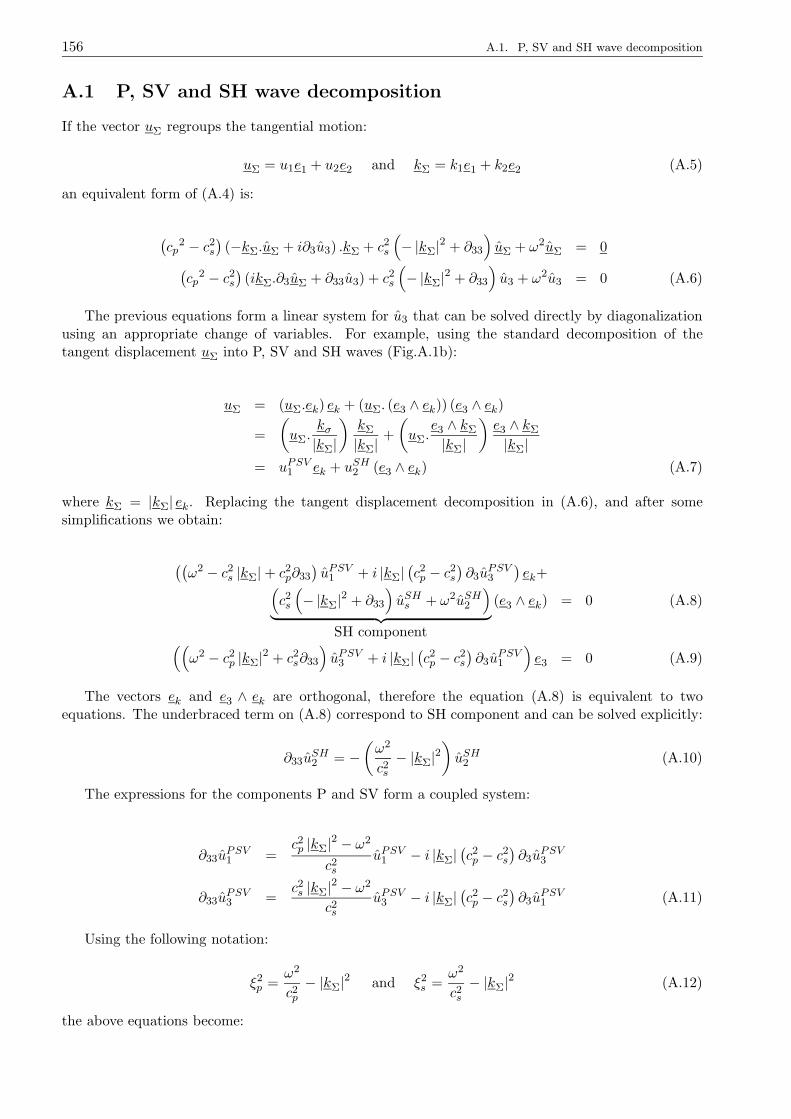
156 A.1. P, SV and SH wave decomposition
A.1 P, SV and SH wave decomposition
If the vector uΣ regroups the tangential motion:
uΣ = u1e1 + u2e2 and kΣ = k1e1 + k2e2 (A.5)
an equivalent form of (A.4) is:
(cp
2 − c2s)(−kΣ.uΣ + i∂3u3) .kΣ + c2s
(
− |kΣ|2 + ∂33
)
uΣ + ω2uΣ = 0
(cp
2 − c2s)(ikΣ.∂3uΣ + ∂33u3) + c2s
(
− |kΣ|2 + ∂33
)
u3 + ω2u3 = 0 (A.6)
The previous equations form a linear system for u3 that can be solved directly by diagonalizationusing an appropriate change of variables. For example, using the standard decomposition of thetangent displacement uΣ into P, SV and SH waves (Fig.A.1b):
uΣ = (uΣ.ek) ek + (uΣ. (e3 ∧ ek)) (e3 ∧ ek)
=
(
uΣ.kσ|kΣ|
)kΣ
|kΣ|+
(
uΣ.e3 ∧ kΣ
|kΣ|
)e3 ∧ kΣ
|kΣ|= uPSV1 ek + uSH2 (e3 ∧ ek) (A.7)
where kΣ = |kΣ| ek. Replacing the tangent displacement decomposition in (A.6), and after somesimplifications we obtain:
((ω2 − c2s |kΣ|+ c2p∂33
)uPSV1 + i |kΣ|
(c2p − c2s
)∂3u
PSV3
)ek+
(
c2s
(
− |kΣ|2 + ∂33
)
uSHs + ω2uSH2
)
︸ ︷︷ ︸
SH component
(e3 ∧ ek) = 0 (A.8)
((
ω2 − c2p |kΣ|2 + c2s∂33
)
uPSV3 + i |kΣ|(c2p − c2s
)∂3u
PSV1
)
e3 = 0 (A.9)
The vectors ek and e3 ∧ ek are orthogonal, therefore the equation (A.8) is equivalent to twoequations. The underbraced term on (A.8) correspond to SH component and can be solved explicitly:
∂33uSH2 = −
(ω2
c2s− |kΣ|2
)
uSH2 (A.10)
The expressions for the components P and SV form a coupled system:
∂33uPSV1 =
c2p |kΣ|2 − ω2
c2suPSV1 − i |kΣ|
(c2p − c2s
)∂3u
PSV3
∂33uPSV3 =
c2s |kΣ|2 − ω2
c2suPSV3 − i |kΣ|
(c2p − c2s
)∂3u
PSV1 (A.11)
Using the following notation:
ξ2p =ω2
c2p− |kΣ|2 and ξ2s =
ω2
c2s− |kΣ|2 (A.12)
the above equations become:
Appendix A. Paraxial approximation 157
∂33uSH2 = 0
∂33uPSV1 = −
c2pc2sξ2pu
PSV1 − i
|kΣ|(c2p − c2s
)
c2s∂3u
PSV3
∂33uPSV3 = −c
2s
c2pξ2s u
PSV2 − i
|kΣ|(c2p − c2s
)
c2p∂3u
PSV1 (A.13)
The solution of the previous differential system can be easy carried out by replacing test solutionsof the form ui = eλxi . This substitution leads to a characteristic polynomial in terms of λ. Aswe are interested only in the solutions propagating downwards (outgoing waves following −e3), onlythe Im(λ) < 0 solutions are kept. Imposing these considerations, the solution for the displacementcomponents are:
uPSV1 = AP e−iξpx3 +ASV e
−iξsx3
uSH2 = ASH e−iξsx3
uPSV3 = − ξp|kΣ|
AP e−iξpx3 +
|kΣ|ξs
ASV e−iξsx3 (A.14)
In order to compute the constants AP , ASH and ASV we suppose to know the displacementus(x3 = 0) over the boundary Σ. Evaluating the system (A.14) for x3 = 0, and imposing the knowndisplacement values uSH2 (x3 = 0), uPSV1 (x3 = 0) and uPSV3 (x3 = 0), we obtain:
ASH = uSH20
AP =|kΣ|2
ξpξs + |kΣ|2uPSV10
− ξs |kΣ|ξpξs |kΣ|2
uPSV30
ASV =ξpξs
ξpξs + |kΣ|uPSV10
+ξs |kΣ|
ξpξs + |kΣ|2uPSV30
(A.15)
A.2 Spectral impedance approximation
In order to construct the impedance over the boundary Σ, we need to evaluate the stress vector t(x, t)applied on the plane perpendicular to e3. As it is assumed that the domain Ωs′ (and Ωst) is elastic:
t (x, t) =(λdiv (us′) I + 2µε
).e3 ∀x ∈ Σ (A.16)
The corresponding expression in frequency domain is:
t (x, ω) = ρc2s (∂3u1 + ik1u3) e1 + ρc2s (∂3u2 + ik2u3) e2
+ρc2p(∂3u3ρ
(c2p − 2c2s
)(ik1u1 + ik2u2)
)e3
= ρc2s (∂3uΣ + iu3kΣ) +(iρ(c2p − 2c2s
)kΣ.uΣ + ρc2p∂3u3
)e3 ∀x ∈ Σ (A.17)
The previous expression can be written in terms of the decomposition into P, SV and SH waves:
t (x, ω) = ρc2s(∂3u
PSV1 + iuPSV3 |kΣ|
)ek + ρc2s∂3u
SH2 (e3 ∧ ek)
+(iρ(c2p − 2c2s
)|kΣ| uPSV1 + ρc2s∂3u
PSV3
)e3 (A.18)
Using the displacement expressions previously obtained (A.14), it is possible to compute directlythe partial derivatives and replace them in (A.18):
158 A.2. Spectral impedance approximation
t (x, ω) =iρ
ξpξs + |kΣ|2(
−ξpω2uPSV10+ c2s |kΣ|
(
|kΣ|2 + 2ξpξs − ξ2s)
uPSV30
)
ek
−iρc2sξsuSH20(e3 ∧ ek) +
iρ
ξpξs + |kΣ|2(
|kΣ|(
ω2 − 2c2s
(
ξpξs + |kΣ|2))
uPSV10− ξsω2uPSV30
)
e3
(A.19)
The previous equation can be written in terms of a linear operator over the displacements at theboundary:
t (x, ω) = A (|kΣ| , ω) .u0 (kΣ, ω) (A.20)
where A (|kΣ| , ω) is the global impedance operator. By using an inverse Fourier transform, the corre-sponding expression in time domain is:
t (x, t) =1
8π3
∫ ∞
−∞A (|kΣ| , ω) u0 (kΣ, ω) ei(kΣ.xΣ+ωt)dkΣ dω (A.21)
The equation (A.21) represents the spectral action imposed by outgoing waves propagating in −e3direction from the boundary Σ. This action is nonlocal since depends on the displacements u0 (kΣ, ω),i.e., the Fourier transform of u (xΣ, t) over the time t and the space xΣ. In order to obtain a localapproximation of the impedance Engquist and Majda (1977) proposed to expand the variables ξp and
ξs as a series of|kΣ|ξ
. For example, using a Taylor’s expansion for ξp:
ξp =ω
cp
√
1−c2pω2|kΣ|2 =
ω
cp
(
1−(cpω|kΣ|
)2 1
2+ . . .
)
(A.22)
Thus, the zero order and first order approximations are given by:
Zero order approximation : ξp =ω
cp+O
(
c2p|kΣ|2ω2
)
(A.23)
First order approximation : ξp =ω
cp
(
1− 1
2
c2pω2|kΣ|2
)
+O(
c4p|kΣ|4ω4
)
(A.24)
The zero order approximation is the familiar solution for the one-dimensional wave propagationproblem and could be easily derived from physical considerations (Wolf, 1985; Wolf and Song, 1996).For the three-dimensional case, the zero order approximation is accurate for high frequency wavesand for waves approximately normal to the boundary Σ (kΣ small). Some numerical instabilities arefound for high-order Taylor expansions (Engquist and Majda, 1977). An expansion using Pade seriesencompasses this problem (Clayton and Engquist, 1977), in this case the series follows the recursiveform:
ξjp =ω
cp
1−
(cp|kΣ|ω
)2
1 +cpωξj−1p
+ . . .
with ξ1p =
ω
cp(A.25)
In order to construct the paraxial approximation for the spectral impedance on the boundary Σ,the expansions for ξp and ξs can be replaced in (A.19). After some simplifications, we obtain for thezero order |kΣ| expansion:
t (x, ω) = −iρcsω(uPSV10
ek + uSH20(e3 ∧ ek)
)− iρcpωuPSV30
e3 ∀x ∈ Σ (A.26)
Appendix A. Paraxial approximation 159
In the local reference system at the boundary (e1, e2, e3), the previous expression becomes:
t (x, ω) = −iρcsωu10e1 − iρcsωu20e2 − iρcpωu30e3 ∀x ∈ Σ (A.27)
Taking inverse Fourier transform, the corresponding expression in time domain is:
t (x, t) = −ρcsu10e1 − ρcsu20e2 − ρcpu30e3 ∀x ∈ Σ (A.28)
If a first order |kΣ| expansion is used, the corresponding stress vector in frequency domain can bewritten as:
t (x, t) = (−iρcsωu10 + iρcs (2cs − cp) u30k1) e1 + (−iρcsωu20 + iρcs (2cs − cp) u30k2) e2
+ (−iρcpωu30 − iρcs (2cs − cp) (u10k1 + u20k2)) e3 ∀ x ∈ Σ (A.29)
The corresponding expression in time domain is:
t (x, t) = (−ρcsu10 + ρcs (2cs − cp) ∂1u30) e1 + (−ρcsu20 + ρcs (2cs − cp) ∂2u30) e2
(−ρcpu30 − ρcs (2cs − cp) (∂1u10 + ∂2u20)) e3 ∀x ∈ Σ (A.30)
It can be noticed that the previous expression is developed using only the first term of the expansion(A.22) for ξp and ξs. In the last expression, the spatial derivatives lead to some numeric instabilities.In this case, high order finite elements must be used to avoid strong discontinuities in the evaluation ofthese terms. A detailed studied of the numerical dispersion of the paraxial approximation dependingon the order of the approximation can be found in Modaressi (1987); de Martin and Aochi (2008).
In a symbolic way, the previous relations in time domain can be summarized in terms of an operatorAn for the n-order approximation over the displacement field us at the boundary Σ of the Ωs domain:
t (x, t) = A0 (us) (A.31)
t (x, t) = A1
(us, ∂xus
)(A.32)
Usually, the total displacement field on the unbounded domain Ωs′ is decomposed into an incidentfield ui and into a radiant field ur:
us′ = ui + ur (A.33)
where the radiant field must vanish far enough from the boundary Σ:
lim‖x‖→∞
ur = 0 (A.34)
At the boundary, the stress vector due to the diffraction can be computed as:
t (ur, t) = A0 (ur) or t (ur, t) = A1
(ur, ∂xur
)(A.35)
Using the continuity of the stress tensor at Σ and the assumption of linear elastic behaviour aroundthe boundary, the zero-order approximation for the total stress vector can be summarized as:
t (us, t) = −t (us′ , t)= −t (ui, t)− t (ur, t)= −t (ui, t)−A0 (ur)
= −t (ui, t)−A0 (us) +A0 (ui) (A.36)
The extension for the case of saturated porous media is presented in Modaressi and Benzenati(1994) for the u−p simplified dynamic Biot formulation. The extension of paraxial absorbing boundaryfor a MESHLESS approach is extensively treated by Aubert (1997).

160 A.2. Spectral impedance approximation

Appendix B
Mechanical interfaces
The model takes into account the normal and the tangential discontinuities over the interface Σbs
between both solid domains Ωb and Ωs. It is assumed that both solid domains are in contact at initialstate and small-strains applies. Let n the normal vector over the interface oriented from Ωb to Ωs.The jump of displacement defined in (1.33) can be decomposed into a normal component (gap [uN ])and a relative tangential jump (slide [uT ]):
[uN ] = [u].n
[uT ] = [u]− [uN ]n (B.1)
If σ is the stress tensor of Ωs or Ωb, the normal stress σN and the tangential stress vector σT overΣbs can be written as (Fig.B.1):
σN = n.σ.n
σT = σ.n− σNn (B.2)
σT
σ.nσNn
n
Σbs
Figure B.1: Stress vector decomposition over the interface Σbs
According to action-reaction principle, the stress vector must be continuous over the interface evenif uplift or slide appears during the loading (1.32). Therefore, only displacement discontinuities areallowed. Assuming a Mohr-Coulomb frictional behaviour, three different criteria must be satisfied:
1. No interpenetration criterion:[uN ] ≥ 0
2. Uplift and free surface criterion:
If [uN ] > eini → σ.n = 0
where eini is the initial thickness of the interface.
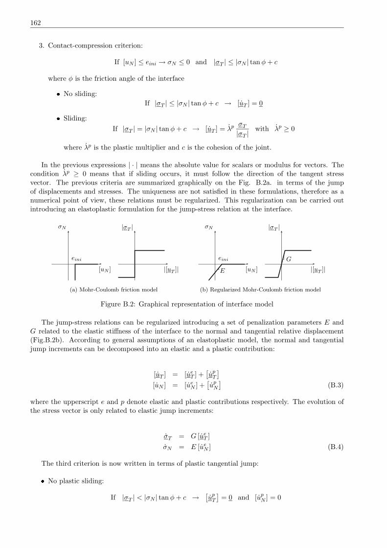
162
3. Contact-compression criterion:
If [uN ] ≤ eini → σN ≤ 0 and |σT | ≤ |σN | tan φ+ c
where φ is the friction angle of the interface No sliding:
If |σT | ≤ |σN | tan φ+ c → [uT ] = 0 Sliding:
If |σT | = |σN | tan φ+ c → [uT ] = λpσT|σT |
with λp ≥ 0
where λp is the plastic multiplier and c is the cohesion of the joint.
In the previous expressions | · | means the absolute value for scalars or modulus for vectors. Thecondition λp ≥ 0 means that if sliding occurs, it must follow the direction of the tangent stressvector. The previous criteria are summarized graphically on the Fig. B.2a. in terms of the jumpof displacements and stresses. The uniqueness are not satisfied in these formulations, therefore as anumerical point of view, these relations must be regularized. This regularization can be carried outintroducing an elastoplastic formulation for the jump-stress relation at the interface.
σN
[uN ]
eini
|σT |
|[uT ]|
(a) Mohr-Coulomb friction model
σN
[uN ]
eini
E
|σT |
|[uT ]|G
(b) Regularized Mohr-Coulomb friction model
Figure B.2: Graphical representation of interface model
The jump-stress relations can be regularized introducing a set of penalization parameters E andG related to the elastic stiffness of the interface to the normal and tangential relative displacement(Fig.B.2b). According to general assumptions of an elastoplastic model, the normal and tangentialjump increments can be decomposed into an elastic and a plastic contribution:
[uT ] = [ueT ] +[upT]
[uN ] = [ueN ] +[upN]
(B.3)
where the upperscript e and p denote elastic and plastic contributions respectively. The evolution ofthe stress vector is only related to elastic jump increments:
σT = G [ueT ]
σN = E [ueN ] (B.4)
The third criterion is now written in terms of plastic tangential jump: No plastic sliding:
If |σT | < |σN | tan φ+ c →[upT]
= 0 and [upN ] = 0
Appendix B. Mechanical interfaces 163 Plastic sliding:If |σT | = |σN | tan φ+ c → ∃ λp ≥ 0 t.q.
[upT]
= λpσT|σT |
[upN]
= λp tanψ
where ψ is the angle of dilatancy of the joint, which relates the plastic normal uplift with the plasticsliding. For a zero value for ψ, the dilatancy vanishes and the formulation is equivalent to a Coulombpure friction model. When φ = ψ, the elastoplastic friction model is associated.
The computation of the plastic multiplier λp can be easy carried out with the compatibility equationderived from the friction threshold:
1
|σT |(σT .σT ) + σN tanφ = 0 (B.5)
Injecting the jump-stress relations (B.4), the previous expression becomes:
G
|σT |(σT . [u
eT ]) + E[ueN ] tan φ = 0 (B.6)
Therefore, the plastic multiplier can be computed as:
λp =
G|σT | (σT . [uT ]) + E [uN ] tan φ
G+ E tan φ tanψ(B.7)
Finally, the total stress increment at the joint is given by:
σT = G [uT ]− λpG σT|σT |
σN = E[uN ]− λpE tanψ (B.8)
B.1 Numerical integration
The integration of the constitutive model is carried out following an explicit strategy. During a loadstep n + 1, the total jump increment is divided in two parts: the first one correspond to elastic partbefore reaching the limit of elasticity, and the second one is plastic increment. For an iteration k + 1of the loading step n, the jump increments can be written as:
[uT ] = 1∆t
[
uk+1Tn+1
− uTn
]
=1
∆t[∆uT ]
[uN ] = 1∆t
[
uk+1Nn+1
− uNn
]
=1
∆t[∆uN ] (B.9)
where the time step increment ∆t is assumed to be constant during the analysis. Afterward, the stepincrement is divided in two parts: γ∆t and (1− γ) ∆t. The first one is the elastic part of the incrementand second one the corresponding plastic part. The value of γ is computed as:
f(σTn
+ γ∆σT , σNn + γ∆σN)≤ 0 (B.10)
where:
f (σT , σN ) = |σT | − |σn| tanφ∆σT = G [∆uT ]
∆σn = E [∆un]

164 B.1. Numerical integration
With γ, the elastic part of stress increment is known. Next, the plastic multiplier λp is computedwith (B.7) using the plastic part of the jump increment:
[∆u∗T ] = (1− γ) [∆uT ]
[∆uN ]∗ = (1− γ) [∆uN ] (B.11)
for stress state:
σ∗T = σTn+ γ∆σT
σ∗N = σNn + γ∆σN (B.12)
After the evaluation of the plastic multiplier, the stress increment can be written in a matrix form:
∆σT∆σN
=
G− (1−γ)G2
H− (1−γ)EG tanφ
H
− (1−γ)EG tanφH
E − (1−γ)E2 tanφ tanψH
[∆uT ]∗
[∆uN ]∗
(B.13)
where H = G+ E tanφ tanψ. Finally, the stress tensor at the interface for the iteration k + 1 of theload step n+ 1 is obtained by:
σk+1Tn+1
= σTn+ ∆σT (B.14)
σk+1Nn+1
= σNn + ∆σN (B.15)
The model parameters for the mechanical joint element are summarized in Table B.1.
Table B.1: Parameters for the Mohr-Coulomb joint constitutive model
Parameter Description
E normal stiffness modulus
G tangent stiffness modulus
φ friction angle
ψ dilatancy angle
eini joint thickness
c joint cohesion
Appendix C
Continuous beam constitutive model
According to beam kinematics introduced in §1.2, assuming the transverse stresses are small withrespect to axial stress σ
ber and the material is isotropic and elastic, the axial stress vector can be
computed as:
σber =
(
C : ε
)
er
=
(
C : (∂ru0rer + ∂ru1 ∧ x∗)⊗s e3)
er (C.1)
where C is the elastic tensor of the material. In this work we are interested in material non-linear
behaviour, in this case, the axial stress vector can be written symbolically as:
σber = σ
b
(ε)er = σ
b((∂ru0rer + ∂ru1 ∧ x∗)⊗s e3) er (C.2)
It can be noticed that according to the this kinematics, the stress tensor can be written as:
σb= σrr er ⊗ er + σrs er ⊗s es + σrt er ⊗s et (C.3)
C.1 Non-linear constitutive model
The non-linear material behavior is modelled by a Prandtl-Reuss elastoplastic constitutive model(Lemaitre and Chaboche, 2001; Chen and Mizuno, 1990) with a Von Mises yield criterion and isotropichardening. Plastic incompressibility is assumed, i.e. the yield function f depends only of the invariantsof the deviatoric stress tensor s:
f(
σb, ǫp)
= σeq −R− σy =√
3J2
(s)− k(ǫp)− σy (C.4)
where J2 is the second invariant of s, R = k(ǫp) is the isotropic hardening rule in terms of thecumulative plastic strain ǫp:
ǫp =
∫ t
0
√
εp(τ) : εp(τ) dτ
and σy is the initial elastic limit stress. An associated flow rule and a normal hardening rule are used:
εp = λp∂f
∂σb
=3
2σeqλp s
ǫp = −λ ∂f∂R
= λp (C.5)
According to Bernouilli beams kinematics, the explicit form of s is given by:
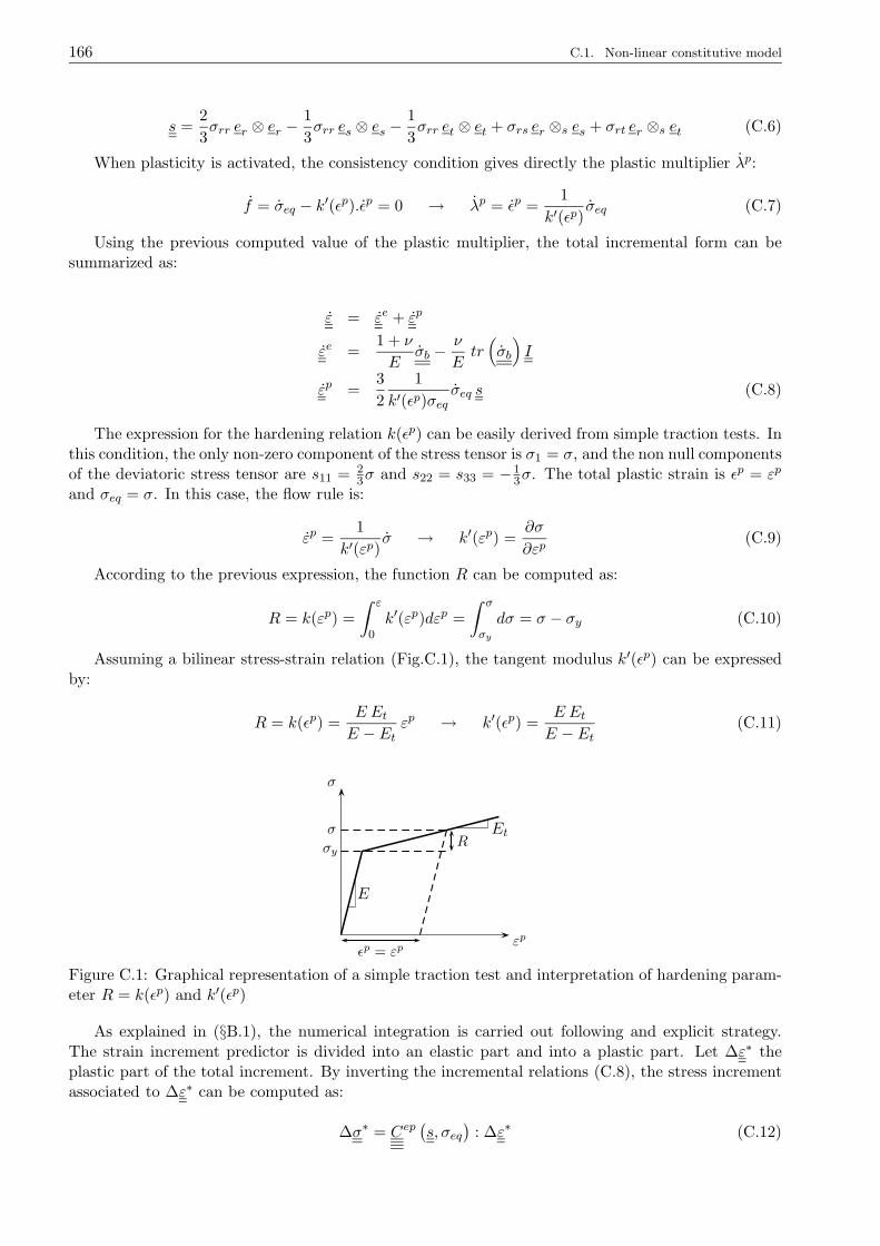
166 C.1. Non-linear constitutive model
s =2
3σrr er ⊗ er −
1
3σrr es ⊗ es −
1
3σrr et ⊗ et + σrs er ⊗s es + σrt er ⊗s et (C.6)
When plasticity is activated, the consistency condition gives directly the plastic multiplier λp:
f = σeq − k′(ǫp).ǫp = 0 → λp = ǫp =1
k′(ǫp)σeq (C.7)
Using the previous computed value of the plastic multiplier, the total incremental form can besummarized as:
ε = εe + εp
εe =1 + ν
Eσb −
ν
Etr(
σb
)
I
εp =3
2
1
k′(ǫp)σeqσeq s (C.8)
The expression for the hardening relation k(ǫp) can be easily derived from simple traction tests. Inthis condition, the only non-zero component of the stress tensor is σ1 = σ, and the non null componentsof the deviatoric stress tensor are s11 = 2
3σ and s22 = s33 = −13σ. The total plastic strain is ǫp = εp
and σeq = σ. In this case, the flow rule is:
εp =1
k′(εp)σ → k′(εp) =
∂σ
∂εp(C.9)
According to the previous expression, the function R can be computed as:
R = k(εp) =
∫ ε
0k′(εp)dεp =
∫ σ
σy
dσ = σ − σy (C.10)
Assuming a bilinear stress-strain relation (Fig.C.1), the tangent modulus k′(ǫp) can be expressedby:
R = k(ǫp) =E EtE − Et
εp → k′(ǫp) =E EtE − Et
(C.11)
σ
εp
σy
σR
ǫp = εp
E
Et
Figure C.1: Graphical representation of a simple traction test and interpretation of hardening param-eter R = k(ǫp) and k′(ǫp)
As explained in (§B.1), the numerical integration is carried out following and explicit strategy.The strain increment predictor is divided into an elastic part and into a plastic part. Let ∆ε∗ theplastic part of the total increment. By inverting the incremental relations (C.8), the stress incrementassociated to ∆ε∗ can be computed as:
∆σ∗ = Cep(s, σeq
): ∆ε∗ (C.12)

Appendix C. Continuous beam constitutive model 167
as the elastoplastic tensor Cep is a function of the deviatoric stress tensor, the equivalent stress σeq
and its derivative, the plastic increment is subdivided in several steps and the elastoplastic tensorevaluated for the updated values of s , σeq and dσeq for each step.
The model parameters for the continuous beam element are summarized in the Table C.1. Aspreviously explained, these parameters are related to experimental results of a simple traction test.The numerical used values are given for each example in the corresponding section.
Table C.1: Parameters for the Prandtl-Reuss constitutive model
Parameter Description
E elastic modulus
ν Poisson’s modulus
σy initial yield stress
Et hardening modulus

168 C.1. Non-linear constitutive model
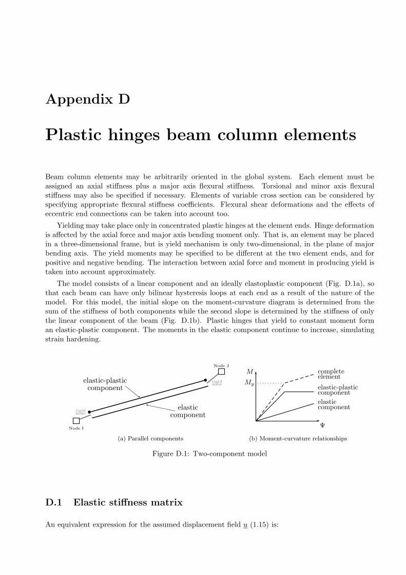
Appendix D
Plastic hinges beam column elements
Beam column elements may be arbitrarily oriented in the global system. Each element must beassigned an axial stiffness plus a major axis flexural stiffness. Torsional and minor axis flexuralstiffness may also be specified if necessary. Elements of variable cross section can be considered byspecifying appropriate flexural stiffness coefficients. Flexural shear deformations and the effects ofeccentric end connections can be taken into account too.
Yielding may take place only in concentrated plastic hinges at the element ends. Hinge deformationis affected by the axial force and major axis bending moment only. That is, an element may be placedin a three-dimensional frame, but is yield mechanism is only two-dimensional, in the plane of majorbending axis. The yield moments may be specified to be different at the two element ends, and forpositive and negative bending. The interaction between axial force and moment in producing yield istaken into account approximately.
The model consists of a linear component and an ideally elastoplastic component (Fig. D.1a), sothat each beam can have only bilinear hysteresis loops at each end as a result of the nature of themodel. For this model, the initial slope on the moment-curvature diagram is determined from thesum of the stiffness of both components while the second slope is determined by the stiffness of onlythe linear component of the beam (Fig. D.1b). Plastic hinges that yield to constant moment forman elastic-plastic component. The moments in the elastic component continue to increase, simulatingstrain hardening.
rigidzone
rigidzone
Node I
Node J
elasticcomponent
elastic-plasticcomponent
(a) Parallel components
Ψ
M
My
elasticcomponent
elastic-plasticcomponent
completeelement
(b) Moment-curvature relationships
Figure D.1: Two-component model
D.1 Elastic stiffness matrix
An equivalent expression for the assumed displacement field u (1.15) is:
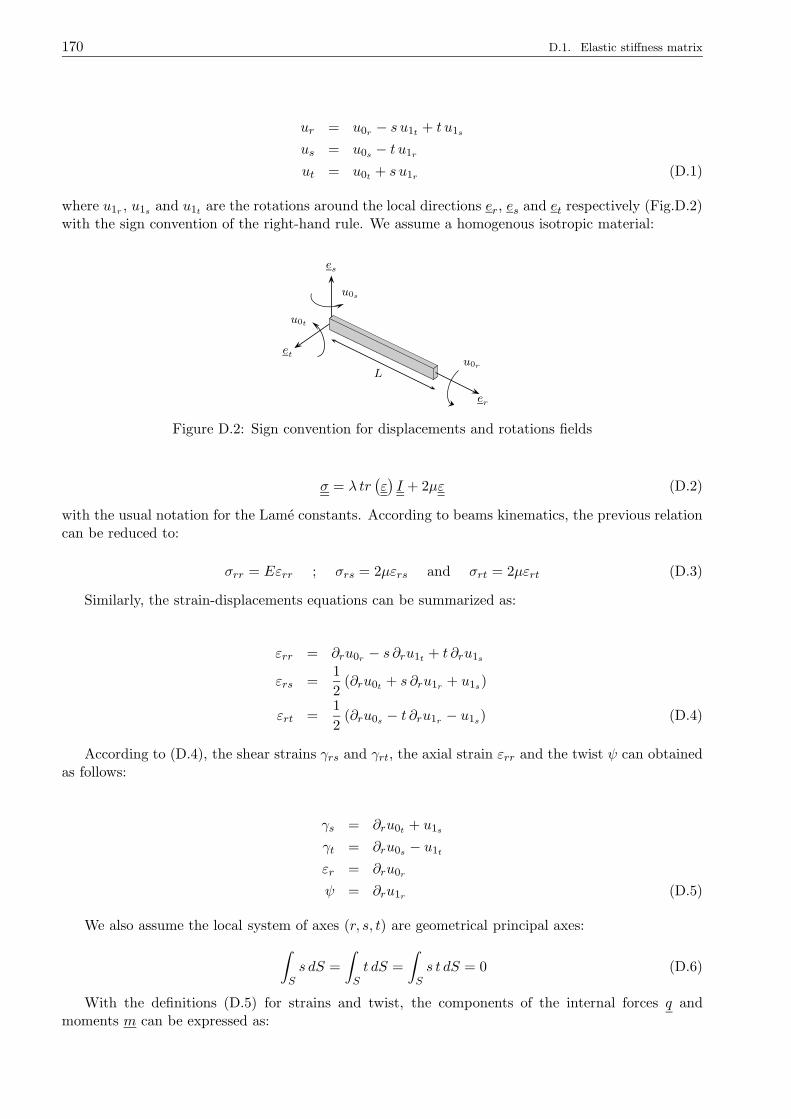
170 D.1. Elastic stiffness matrix
ur = u0r − s u1t + t u1s
us = u0s − t u1r
ut = u0t + s u1r (D.1)
where u1r , u1s and u1t are the rotations around the local directions er, es and et respectively (Fig.D.2)with the sign convention of the right-hand rule. We assume a homogenous isotropic material:
es
et
er
u0r
u0t
u0s
L
Figure D.2: Sign convention for displacements and rotations fields
σ = λ tr(ε)I + 2µε (D.2)
with the usual notation for the Lame constants. According to beams kinematics, the previous relationcan be reduced to:
σrr = Eεrr ; σrs = 2µεrs and σrt = 2µεrt (D.3)
Similarly, the strain-displacements equations can be summarized as:
εrr = ∂ru0r − s ∂ru1t + t ∂ru1s
εrs =1
2(∂ru0t + s ∂ru1r + u1s)
εrt =1
2(∂ru0s − t ∂ru1r − u1s) (D.4)
According to (D.4), the shear strains γrs and γrt, the axial strain εrr and the twist ψ can obtainedas follows:
γs = ∂ru0t + u1s
γt = ∂ru0s − u1t
εr = ∂ru0r
ψ = ∂ru1r (D.5)
We also assume the local system of axes (r, s, t) are geometrical principal axes:
∫
S
s dS =
∫
S
t dS =
∫
S
s t dS = 0 (D.6)
With the definitions (D.5) for strains and twist, the components of the internal forces q andmoments m can be expressed as:
Appendix D. Plastic hinges beam column elements 171
qr =
∫
S
σrr dS =
∫
S
∂ru0r − s∂ru1t + t∂ru1s dS = EAεr
qs =
∫
S
σsr dS = µ
∫
S
∂ru0t + s∂ru1r + u1s dS = µAγs
qt =
∫
S
σst dS = µ
∫
S
∂ru0s − t∂ru1r − u1t dS = µAγt
mr =
∫
S
σrts− σrst dS = µ
∫
S
(∂ru0t + s∂ru1r + u1s) s− (∂ru0s − t∂ru1r − u1t) t dS = µJψ
ms =
∫
S
σrrt dS = E
∫
S
(∂ru0r − s∂ru1t + tu1s) t dS = EIsκs
mt =
∫
S
σrrs dS = E
∫
S
(∂ru0r − s∂ru1t + tu1s) s dS = −EItκt (D.7)
with the standard definitions for area A, moments of inertia Is and It and polar moment of inertia J :
Is =
∫
S
t2 dS ; It =
∫
S
s2 dS and J = Is + It
Decomposing the field test w in a similar manner, it is possible to compute the same expressionfor γrs, γrt, εrr, ψ, κs and κt (denoted with a bar to differentiate with these associated to the realfield u). Injecting these definition in (1.42) we obtain for a linear elastic isotropic beam:
∫
Ωσ : ε dV =
∫
L
(γsµA
ssγs + γtµA
stγt + κsEIsκs + κtEItκt + εrEAεr + ψEJψ
)dl (D.8)
where Ass and Ast are effective shear area for the s and t directions, respectively. Introducing the finiteelement approximation uh0 and uh1 (1.49), the elastic stiffness matrix can be computed straightforward(Hughes, 2000).
D.2 Two-component stiffness matrix
Applying static condensation with respect to bending rotations in the local stiffness matrix defined by(D.8), the local element bending stiffness relationships in r − s plane for the elastic element are:
mI,et
mJ,et
=EItL
[kII kIJkIJ kJJ
]θItθJt
(D.9)
where mI,et and mJ,e
t are the elastic end bending moments at nodes I and J in r− s plane (vectors inet direction), θIt (or u1I3
) and θJt (or u1J3) are the corresponding total end node rotations.
For a linear elastic uniform cross section element, the flexural stiffness coefficients are:
kII = kJJ = 4 and kIJ = 2 (D.10)
Usually it is assumed that the beam has a uniform cross section throughout the length, but elementsof variable cross section can be considered by specifying appropriate flexural stiffness coefficients forthe elastic beam. Elastic shear deformations can be included by specifying an effective shear area Ast .
A plastic hinge forms when the moment in the inelastic component of the element reaches its yieldvalue. A hinge is then introduced into this component, the elastic component remaining unchanged.The measure of flexural plastic deformation is the plastic hinge rotation.
In order to obtain incremental moment-rotation equations, the total end rotation increments mustbe related to rotations in both elastic and elastic-plastic components (Fig.D.3). In this figure mI
t andmJt are the total bending moment at the ends I and J , mI,p
t and mJ,pt are the bending moments at the
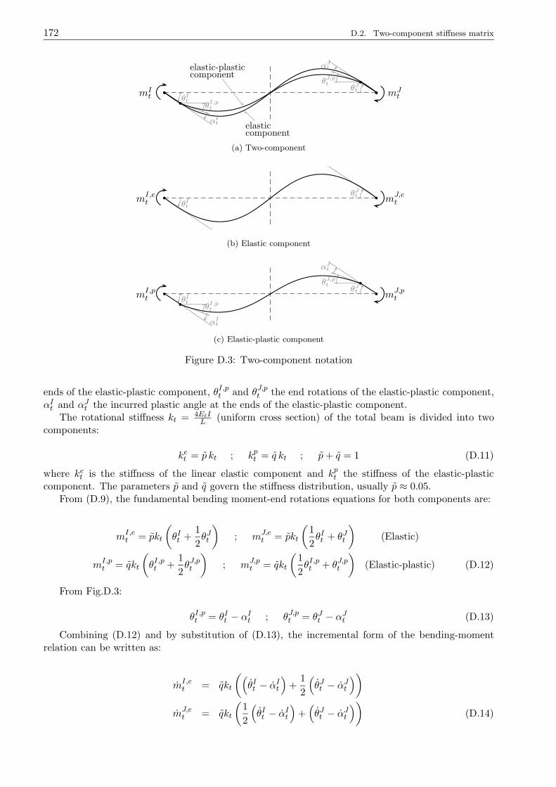
172 D.2. Two-component stiffness matrix
mJtmI
tθJ
t
θIt
θJ,pt
θI,pt
αJt
αIt
elastic-plasticcomponent
elasticcomponent
(a) Two-component
mJ,etmI,e
t
θJt
θIt
(b) Elastic component
mJ,ptmI,p
t
θJt
θIt
θJ,pt
θI,pt
αJt
αIt
(c) Elastic-plastic component
Figure D.3: Two-component notation
ends of the elastic-plastic component, θI,pt and θJ,pt the end rotations of the elastic-plastic component,αIt and αJt the incurred plastic angle at the ends of the elastic-plastic component.
The rotational stiffness kt = 4EtIL
(uniform cross section) of the total beam is divided into twocomponents:
ket = p kt ; kpt = q kt ; p+ q = 1 (D.11)
where ket is the stiffness of the linear elastic component and kpt the stiffness of the elastic-plasticcomponent. The parameters p and q govern the stiffness distribution, usually p ≈ 0.05.
From (D.9), the fundamental bending moment-end rotations equations for both components are:
mI,et = pkt
(
θIt +1
2θJt
)
; mJ,et = pkt
(1
2θIt + θJt
)
(Elastic)
mI,pt = qkt
(
θI,pt +1
2θJ,pt
)
; mJ,pt = qkt
(1
2θI,pt + θJ,pt
)
(Elastic-plastic) (D.12)
From Fig.D.3:
θI,pt = θIt − αIt ; θJ,pt = θJt − αJt (D.13)
Combining (D.12) and by substitution of (D.13), the incremental form of the bending-momentrelation can be written as:
mI,et = qkt
((
θIt − αIt)
+1
2
(
θJt − αJt))
mJ,et = qkt
(1
2
(
θIt − αIt)
+(
θJt − αJt))
(D.14)

Appendix D. Plastic hinges beam column elements 173
The addition of bending moments at the ends of the elastic and the elastic-plastic componentsgives the total bending moment:
mIt = mI,e
t +mI,pt ; mJ
t = mJ,et +mJ,p
t (D.15)
Finally, the fundamental bending-end rotation equations for the complete element are obtained:
mIt = kt
((
θIt − qαIt)
+1
2
(
θJt − qαJt))
mJt = kt
(1
2
(
θIt − qαIt)
+(
θJt − qαJt))
(D.16)
Assuming that the state of yield remains constant throughout each time increment, the incrementalbending moments mI
t and mJt are related to both incremental rotations θIt and θJt , and the incremental
plastic angles αIt and αJt . Now, for any state of yield which is held constant throughout a time
increment, it is possible to establish equations of the form αt = αt
(
θIt , θJt
)
relating the incremental
plastic angles to the incremental end rotations. With these equations it is possible to eliminate theincremental plastic angles from the incremental moment-rotation equations resulting in equations of
the form mt = mt
(
θIt , θJt
)
.
When the state of yield is linear at end I or end J , or both, the corresponding incremental plasticangle must be zero: αIt = αJt = 0.
When the state of yield is non-linear at end I or end J , or both, the corresponding incrementaltotal bending moments equals the incremental bending moment of the linear component, and theincremental bending moment in the elastoplastic component is zero: at end I, mI
t = mI,et and mI,p
t = 0;
or at end J , mJt = mJ,e
t and mJ,pt = 0; or both.
On the other hand, mI,et and mJ,e
t are dependent upon the same stiffness parameter p. Conse-quently, this model can have hysteresis loops at the ends with only two slopes kt and pkt although theyields levels may be different.
There are four possible states of yield for a beam:
(a) Linear at ends I and J .
(b) Non-linear at end I and linear at end J .
(c) Linear at end I and non-linear at end J .
(d) Non-linear at ends I and J .
Because the incremental bending moment-end rotation equations have a regular pattern for allfour states of yield, the following matrix equations using the effective stiffness parameters SA, SB andSC can be established (Table D.1):
mIt
mJt
=
[SA SBSB SC
]θItθJt
(D.17)
Even if the beam element can be placed arbitrarily in 3D, this two-component approach is takeninto account only in the local r−s plane (primary flexural plane), therefore the model is bidimensionalin a non-linear sense. The minor axis flexural stiffness (plane r − t) can be obtained by multiplyingthe primary elastic stiffness by a specified factor α. The torsional deformation is related to torque mr
by:
mr =µJ
Lα (D.18)
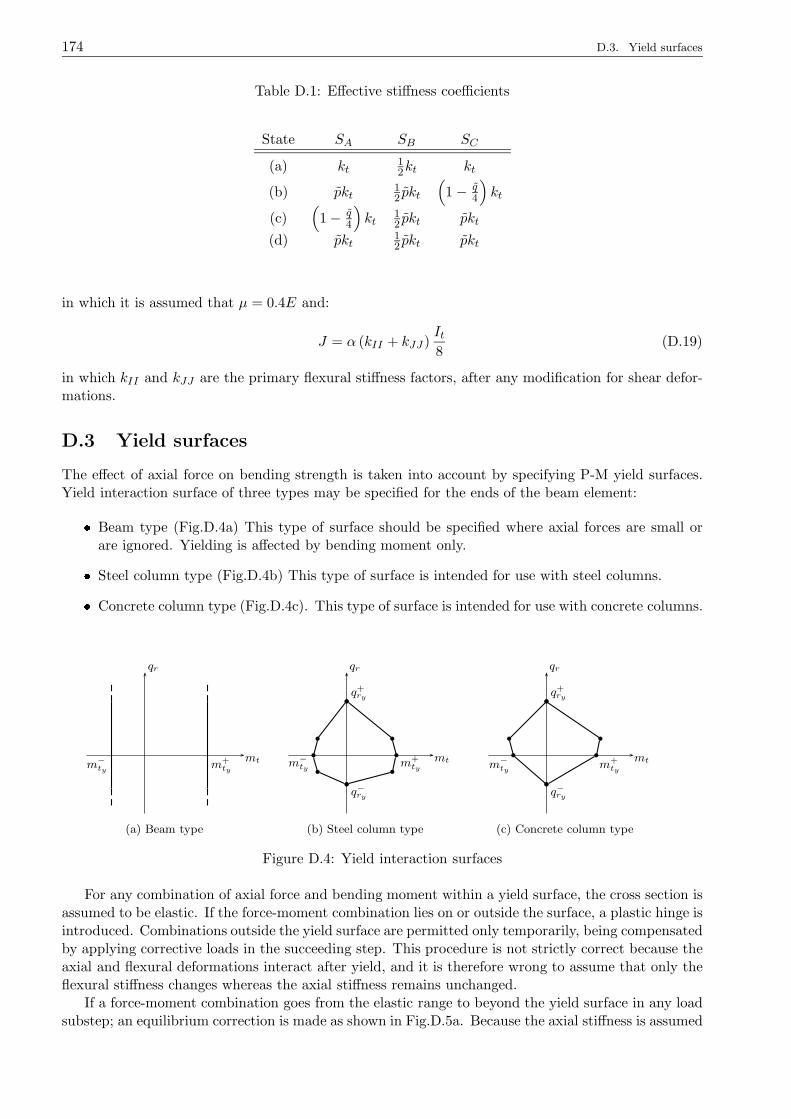
174 D.3. Yield surfaces
Table D.1: Effective stiffness coefficients
State SA SB SC
(a) kt12kt kt
(b) pkt12 pkt
(
1− q4
)
kt
(c)(
1− q4
)
kt12 pkt pkt
(d) pkt12 pkt pkt
in which it is assumed that µ = 0.4E and:
J = α (kII + kJJ )It8
(D.19)
in which kII and kJJ are the primary flexural stiffness factors, after any modification for shear defor-mations.
D.3 Yield surfaces
The effect of axial force on bending strength is taken into account by specifying P-M yield surfaces.Yield interaction surface of three types may be specified for the ends of the beam element: Beam type (Fig.D.4a) This type of surface should be specified where axial forces are small or
are ignored. Yielding is affected by bending moment only. Steel column type (Fig.D.4b) This type of surface is intended for use with steel columns. Concrete column type (Fig.D.4c). This type of surface is intended for use with concrete columns.
mt
qr
m−
tym+
ty
(a) Beam type
mt
qr
q−ry
m−
ty
q+ry
m+ty
(b) Steel column type
mt
qr
q−ry
m−
ty
q+ry
m+ty
(c) Concrete column type
Figure D.4: Yield interaction surfaces
For any combination of axial force and bending moment within a yield surface, the cross section isassumed to be elastic. If the force-moment combination lies on or outside the surface, a plastic hinge isintroduced. Combinations outside the yield surface are permitted only temporarily, being compensatedby applying corrective loads in the succeeding step. This procedure is not strictly correct because theaxial and flexural deformations interact after yield, and it is therefore wrong to assume that only theflexural stiffness changes whereas the axial stiffness remains unchanged.
If a force-moment combination goes from the elastic range to beyond the yield surface in any loadsubstep; an equilibrium correction is made as shown in Fig.D.5a. Because the axial stiffness is assumed
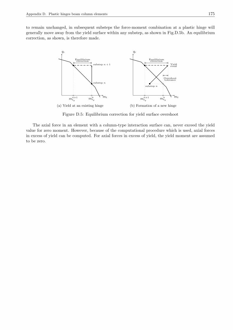
Appendix D. Plastic hinges beam column elements 175
to remain unchanged, in subsequent substeps the force-moment combination at a plastic hinge willgenerally move away from the yield surface within any substep, as shown in Fig.D.5b. An equilibriumcorrection, as shown, is therefore made.
mt
qr
mn+1ty
mnty
substep n
substep n + 1
Equilibriumcorrection
(a) Yield at an existing hinge
mt
qr
mntymn+1
ty
substep n
Yieldevent
Equilibriumcorrection
Overshoottolerance
(b) Formation of a new hinge
Figure D.5: Equilibrium correction for yield surface overshoot
The axial force in an element with a column-type interaction surface can, never exceed the yieldvalue for zero moment. However, because of the computational procedure which is used, axial forcesin excess of yield can be computed. For axial forces in excess of yield, the yield moment are assumedto be zero.

176 D.3. Yield surfaces
Appendix E
ECP multimechanism model
E.1 General hypotheses and characteristics of the model
E.1.1 Hypothesis 1
We assume that small-strains hypothesis is valid, i.e. the strain tensor increment can be decomposedinto an elastic part and a plastic part:
ε = εe + εp (E.1)
consequently, the decomposition is also valid for volumetric εv and deviatoric strains ˙ε increments:
εv = εev + εpv and ˙ε = ˙εe+ ˙ε
p(E.2)
E.1.2 Hypothesis 2
The effective stress principle applies.
E.1.3 Hypothesis 3
The elastic part of the behavior is isotropic:
εev =1
K (p′)p′
˙εe
=1
2G (p′)s (E.3)
where the bulk K = K(p′) and shear G = G(p′) moduli are function of the mean effective compressivestress p′ by a non-linear relation:
K = Kref
(
p′
p′ref
)ne
G = Gref
(
p′
p′ref
)ne
(E.4)
where Kref and Gref are the bulk and shear moduli measured at the mean effective pressure p′ref andne is the degree of non-linearity. Therefore, there is no-coupling effect between the volumetric anddeviatoric elastic strain rates, i.e. εev is independent of ˙ε
e, but ˙ε
edepends on εev.
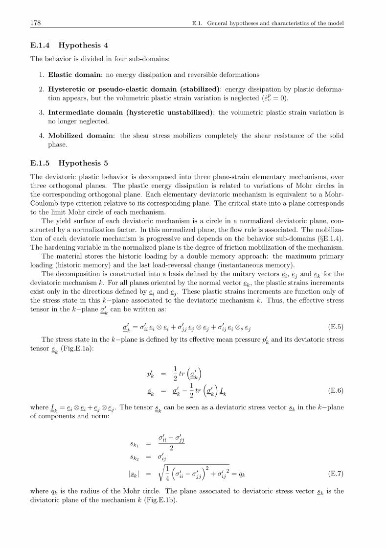
178 E.1. General hypotheses and characteristics of the model
E.1.4 Hypothesis 4
The behavior is divided in four sub-domains:
1. Elastic domain: no energy dissipation and reversible deformations
2. Hysteretic or pseudo-elastic domain (stabilized): energy dissipation by plastic deforma-tion appears, but the volumetric plastic strain variation is neglected (εpv = 0).
3. Intermediate domain (hysteretic unstabilized): the volumetric plastic strain variation isno longer neglected.
4. Mobilized domain: the shear stress mobilizes completely the shear resistance of the solidphase.
E.1.5 Hypothesis 5
The deviatoric plastic behavior is decomposed into three plane-strain elementary mechanisms, overthree orthogonal planes. The plastic energy dissipation is related to variations of Mohr circles inthe corresponding orthogonal plane. Each elementary deviatoric mechanism is equivalent to a Mohr-Coulomb type criterion relative to its corresponding plane. The critical state into a plane correspondsto the limit Mohr circle of each mechanism.
The yield surface of each deviatoric mechanism is a circle in a normalized deviatoric plane, con-structed by a normalization factor. In this normalized plane, the flow rule is associated. The mobiliza-tion of each deviatoric mechanism is progressive and depends on the behavior sub-domains (§E.1.4).The hardening variable in the normalized plane is the degree of friction mobilization of the mechanism.
The material stores the historic loading by a double memory approach: the maximum primaryloading (historic memory) and the last load-reversal change (instantaneous memory).
The decomposition is constructed into a basis defined by the unitary vectors ei, ej and ek for thedeviatoric mechanism k. For all planes oriented by the normal vector ek, the plastic strains incrementsexist only in the directions defined by ei and ej . These plastic strains increments are function only ofthe stress state in this k−plane associated to the deviatoric mechanism k. Thus, the effective stresstensor in the k−plane σ′
kcan be written as:
σ′k
= σ′ii ei ⊗ ei + σ′jj ej ⊗ ej + σ′ij ei ⊗s ej (E.5)
The stress state in the k−plane is defined by its effective mean pressure p′k and its deviatoric stresstensor s
k(Fig.E.1a):
p′k =1
2tr(
σ′k
)
sk
= σ′k− 1
2tr(
σ′k
)
Ik
(E.6)
where Ik
= ei⊗ ei + ej ⊗ ej . The tensor sk
can be seen as a deviatoric stress vector sk in the k−planeof components and norm:
sk1 =σ′ii − σ′jj
2sk2 = σ′ij
|sk| =
√
1
4
(
σ′ii − σ′jj)2
+ σ′ij2 = qk (E.7)
where qk is the radius of the Mohr circle. The plane associated to deviatoric stress vector sk is thediviatoric plane of the mechanism k (Fig.E.1b).
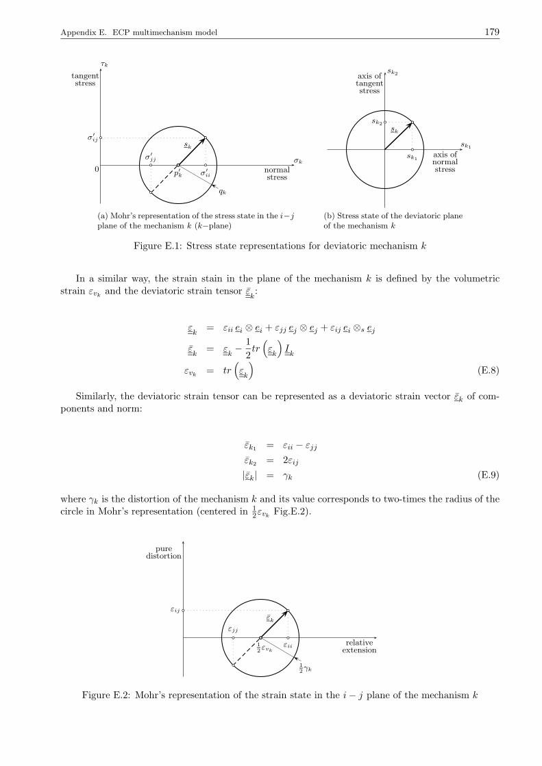
Appendix E. ECP multimechanism model 179
σk
0
τk
tangentstress
normalstress
qk
sk
σ′
ij
σ′
ii
σ′
jj
p′k
(a) Mohr’s representation of the stress state in the i−jplane of the mechanism k (k−plane)
sk1
sk2axis oftangentstress
axis ofnormalstress
sk
sk2
sk1
(b) Stress state of the deviatoric planeof the mechanism k
Figure E.1: Stress state representations for deviatoric mechanism k
In a similar way, the strain stain in the plane of the mechanism k is defined by the volumetricstrain εvk
and the deviatoric strain tensor εk:
εk
= εii ei ⊗ ei + εjj ej ⊗ ej + εij ei ⊗s ejεk
= εk− 1
2tr(
εk
)
Ik
εvk= tr
(
εk
)
(E.8)
Similarly, the deviatoric strain tensor can be represented as a deviatoric strain vector εk of com-ponents and norm:
εk1 = εii − εjjεk2 = 2εij
|εk| = γk (E.9)
where γk is the distortion of the mechanism k and its value corresponds to two-times the radius of thecircle in Mohr’s representation (centered in 1
2εvkFig.E.2).
puredistortion
relativeextension
12γk
εk
εij
εii
εjj
12εvk
Figure E.2: Mohr’s representation of the strain state in the i− j plane of the mechanism k
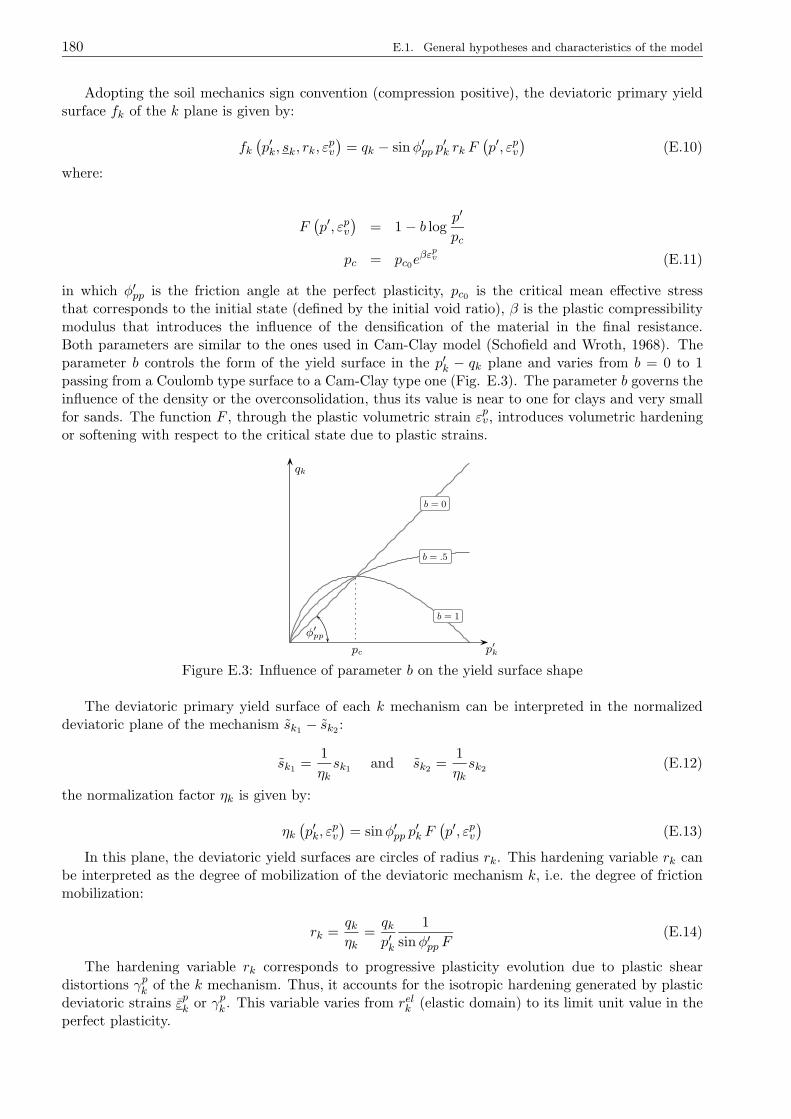
180 E.1. General hypotheses and characteristics of the model
Adopting the soil mechanics sign convention (compression positive), the deviatoric primary yieldsurface fk of the k plane is given by:
fk(p′k, sk, rk, ε
pv
)= qk − sinφ′pp p
′k rk F
(p′, εpv
)(E.10)
where:
F(p′, εpv
)= 1− b log
p′
pc
pc = pc0eβε
pv (E.11)
in which φ′pp is the friction angle at the perfect plasticity, pc0 is the critical mean effective stressthat corresponds to the initial state (defined by the initial void ratio), β is the plastic compressibilitymodulus that introduces the influence of the densification of the material in the final resistance.Both parameters are similar to the ones used in Cam-Clay model (Schofield and Wroth, 1968). Theparameter b controls the form of the yield surface in the p′k − qk plane and varies from b = 0 to 1passing from a Coulomb type surface to a Cam-Clay type one (Fig. E.3). The parameter b governs theinfluence of the density or the overconsolidation, thus its value is near to one for clays and very smallfor sands. The function F , through the plastic volumetric strain εpv, introduces volumetric hardeningor softening with respect to the critical state due to plastic strains.
qk
p′kpc
φ′
pp
b = 1
b = .5
b = 0
Figure E.3: Influence of parameter b on the yield surface shape
The deviatoric primary yield surface of each k mechanism can be interpreted in the normalizeddeviatoric plane of the mechanism sk1 − sk2 :
sk1 =1
ηksk1 and sk2 =
1
ηksk2 (E.12)
the normalization factor ηk is given by:
ηk(p′k, ε
pv
)= sinφ′pp p
′k F
(p′, εpv
)(E.13)
In this plane, the deviatoric yield surfaces are circles of radius rk. This hardening variable rk canbe interpreted as the degree of mobilization of the deviatoric mechanism k, i.e. the degree of frictionmobilization:
rk =qkηk
=qkp′k
1
sinφ′pp F(E.14)
The hardening variable rk corresponds to progressive plasticity evolution due to plastic sheardistortions γpk of the k mechanism. Thus, it accounts for the isotropic hardening generated by plasticdeviatoric strains εpk or γpk . This variable varies from relk (elastic domain) to its limit unit value in theperfect plasticity.
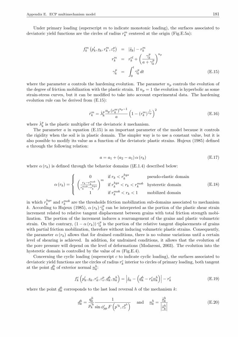
Appendix E. ECP multimechanism model 181
Under primary loading (superscript m to indicate monotonic loading), the surfaces associated todeviatoric yield functions are the circles of radius rmk centered at the origin (Fig.E.5a):
fmk(p′k, sk, r
mk , ε
pv
)= |sk| − rmk
rmk = relk +
(γpk
a+ γpk
)np
γpk =
∫ t
0γpk dt (E.15)
where the parameter a controls the hardening evolution. The parameter np controls the evolution ofthe degree of friction mobilization with the plastic strain. If np = 1 the evolution is hyperbolic as somestrain-stress curves, but it can be modified to take into account experimental data. The hardeningevolution rule can be derived from (E.15):
rmk = λpknp (rmk )np−1
a
(
1− (rmk )1
np
)2
(E.16)
where λpk is the plastic multiplier of the deviatoric k mechanism.
The parameter a in equation (E.15) is an important parameter of the model because it controlsthe rigidity when the soil is in plastic domain. The simpler way is to use a constant value, but it isalso possible to modify its value as a function of the deviatoric plastic strains. Hujeux (1985) defineda through the following relation:
a = a1 + (a2 − a1)α (rk) (E.17)
where α (rk) is defined through the behavior domains (§E.1.4) described below:
α (rk) =
0 if rk < rhysk pseudo-elastic domain(
rk−rmobk
rmobk
−rhysk
)m
if rhysk < rk < rmobk hysteretic domain
1 if rmobk < rk < 1 mobilized domain
(E.18)
in which rhysk and rmobk are the thresholds friction mobilization sub-domains associated to mechanismk. According to Hujeux (1985), α (rk) γ
pk can be interpreted as the portion of the plastic shear strain
increment related to relative tangent displacement between grains with total friction strength mobi-lization. The portion of the increment induces a rearrangement of the grains and plastic volumetricstrain. On the contrary, (1− α (rk)) γ
pk is the portion of the relative tangent displacements of grains
with partial friction mobilization, therefore without inducing volumetric plastic strains. Consequently,the parameter α (rk) allows that for drained conditions, there is no volume variations until a certainlevel of shearing is achieved. In addition, for undrained conditions, it allows that the evolution ofthe pore pressure will depend on the level of deformations (Modaressi, 2003). The evolution into thehysteretic domain is controlled by the value of m (Fig.E.4).
Concerning the cyclic loading (superscript c to indicate cyclic loading), the surfaces associated todeviatoric yield functions are the circles of radius rck interior to circles of primary loading, both tangentat the point dhk of exterior normal nhk:
f ck
(
p′k, sk, rck, ε
pv , d
hk , n
hk
)
=∣∣∣sk −
(
dhk − rcknhk)∣∣∣− rck (E.19)
where the point dhk corresponds to the last load reversal h of the mechanism k:
dhk =qhkp′hk
1
sinφ′pp F(
p′h, εp
h
v
) and nhk =shk∣∣∣shk
∣∣∣
(E.20)
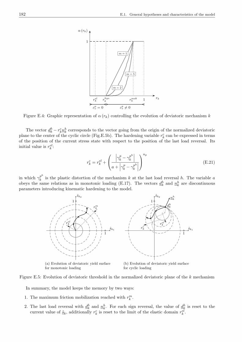
182 E.1. General hypotheses and characteristics of the model
1
α (rk)
rkrelk r
hysk rmob
k 1
m = 1
m = 2
m = 5
εpv = 0 εp
v 6= 0
Figure E.4: Graphic representation of α (rk) controlling the evolution of deviatoric mechanism k
The vector dhk − rcknhk corresponds to the vector going from the origin of the normalized deviatoricplane to the center of the cyclic circle (Fig.E.5b). The hardening variable rck can be expressed in termsof the position of the current stress state with respect to the position of the last load reversal. Itsinitial value is relk :
rck = relk +
∣∣∣γpk − γ
ph
k
∣∣∣
a+∣∣∣γpk − γ
ph
k
∣∣∣
np
(E.21)
in which γph
k is the plastic distortion of the mechanism k at the last load reversal h. The variable aobeys the same relations as in monotonic loading (E.17). The vectors dhk and nhk are discontinuousparameters introducing kinematic hardening to the model.
sk1
sk2
1
1
relk
rmk
b
b
b
(a) Evolution of deviatoric yield surfacefor monotonic loading
sk1
sk2
1
1dh
k
relk
nhk
rck
b
b
b
b
bb
b
b
(b) Evolution of deviatoric yield surfacefor cyclic loading
Figure E.5: Evolution of deviatoric threshold in the normalized deviatoric plane of the k mechanism
In summary, the model keeps the memory by two ways:
1. The maximum friction mobilization reached with rmk .
2. The last load reversal with dhk and nhk. For each sign reversal, the value of dhk is reset to thecurrent value of sk, additionally rck is reset to the limit of the elastic domain relk .
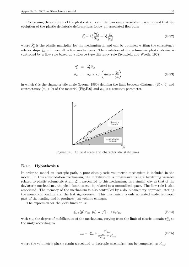
Appendix E. ECP multimechanism model 183
Concerning the evolution of the plastic strains and the hardening variables, it is supposed that theevolution of the plastic deviatoric deformations follow an associated flow rule:
˙εpk = λpk
∂fk∂sk
= λpksk|sk|
(E.22)
where λpk is the plastic multiplier for the mechanism k, and can be obtained writing the consistency
relationships fk = 0 over all active mechanisms. The evolution of the volumetric plastic strains iscontrolled by a flow rule based on a Roscoe-type dilatancy rule (Schofield and Wroth, 1968):
εpk = λpkΨk
Ψk = αψ α (rk)
(
sinψ − qkpk
)
(E.23)
in which ψ is the characteristic angle (Luong, 1980) defining the limit between dilatancy (εpv < 0) andcontractancy (εpv > 0) of the material (Fig.E.6) and αψ is a constant parameter.
ψ
contractancedomain
φ′
pp
dilatancydomain
qk
p′k
criti
cal s
tate
line
characte
ristic sta
te line
Figure E.6: Critical state and characteristic state lines
E.1.6 Hypothesis 6
In order to model an isotropic path, a pure elato-plastic volumetric mechanism is included in themodel. In this consolidation mechanism, the mobilization is progressive using a hardening variablerelated to plastic volumetric strain εpviso associated to this mechanism. In a similar way as that of thedeviatoric mechanisms, the yield function can be related to a normalized space. The flow-rule is alsoassociated. The memory of the mechanism is also controlled by a double-memory approach, storingthe monotonic loading and the last sign-reversal. This mechanism is only activated under isotropicpart of the loading and it produces just volume changes.
The expression for the yield function is:
fiso(p′, riso, pc
)=∣∣p′∣∣− d pc riso (E.24)
with riso the degree of mobilization of the mechanism, varying from the limit of elastic domain reliso tothe unity according to:
riso = reliso +εpviso
c pc
p′ref
+ εpviso
(E.25)
where the volumetric plastic strain associated to isotropic mechanism can be computed as εpviso :
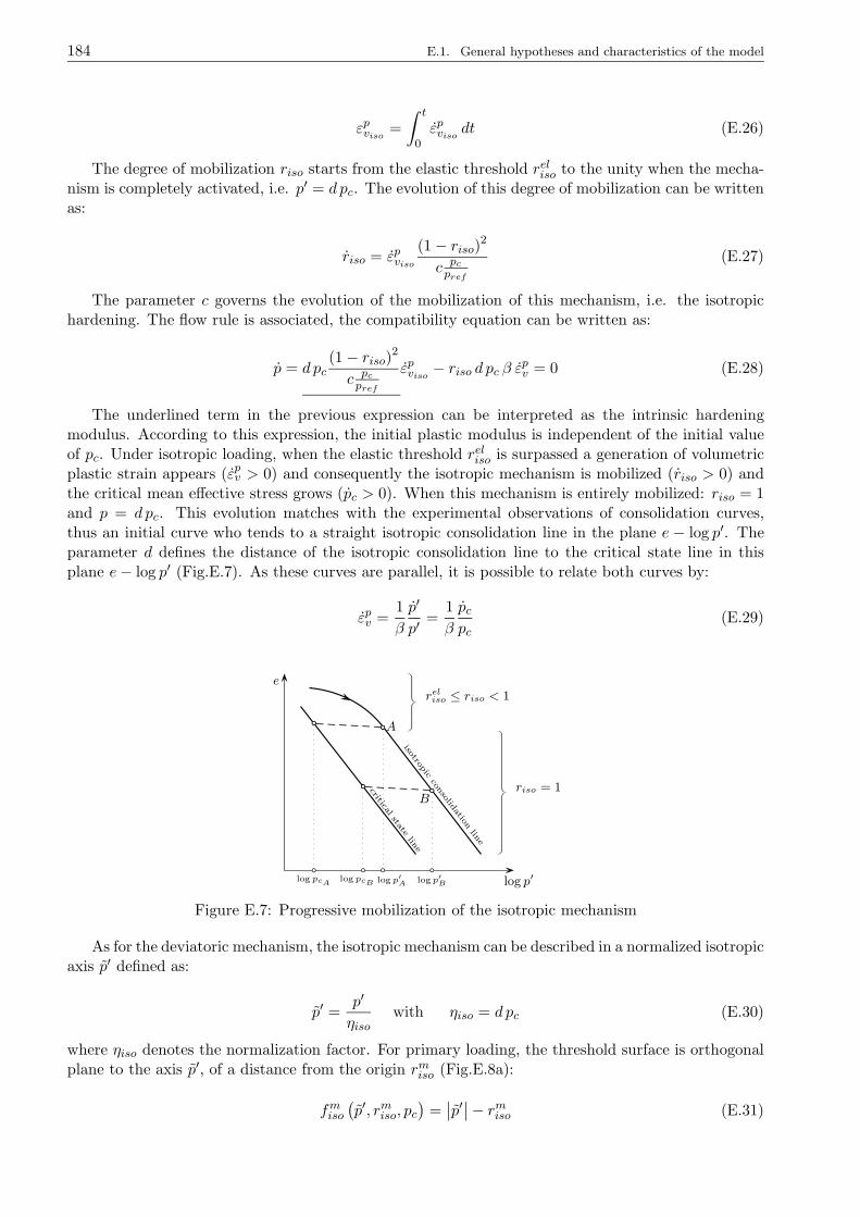
184 E.1. General hypotheses and characteristics of the model
εpviso=
∫ t
0εpviso
dt (E.26)
The degree of mobilization riso starts from the elastic threshold reliso to the unity when the mecha-nism is completely activated, i.e. p′ = d pc. The evolution of this degree of mobilization can be writtenas:
riso = εpviso
(1− riso)2c pc
pref
(E.27)
The parameter c governs the evolution of the mobilization of this mechanism, i.e. the isotropichardening. The flow rule is associated, the compatibility equation can be written as:
p = d pc(1− riso)2c pc
pref
εpviso− riso d pc β εpv = 0 (E.28)
The underlined term in the previous expression can be interpreted as the intrinsic hardeningmodulus. According to this expression, the initial plastic modulus is independent of the initial valueof pc. Under isotropic loading, when the elastic threshold reliso is surpassed a generation of volumetricplastic strain appears (εpv > 0) and consequently the isotropic mechanism is mobilized (riso > 0) andthe critical mean effective stress grows (pc > 0). When this mechanism is entirely mobilized: riso = 1and p = d pc. This evolution matches with the experimental observations of consolidation curves,thus an initial curve who tends to a straight isotropic consolidation line in the plane e − log p′. Theparameter d defines the distance of the isotropic consolidation line to the critical state line in thisplane e− log p′ (Fig.E.7). As these curves are parallel, it is possible to relate both curves by:
εpv =1
β
p′
p′=
1
β
pcpc
(E.29)
e
log p′
criticalstate
line
isotropic
consolid
ationlin
e
A
B
log pcAlog pcB log p′
A log p′
B
reliso ≤ riso < 1
riso = 1
Figure E.7: Progressive mobilization of the isotropic mechanism
As for the deviatoric mechanism, the isotropic mechanism can be described in a normalized isotropicaxis p′ defined as:
p′ =p′
ηisowith ηiso = d pc (E.30)
where ηiso denotes the normalization factor. For primary loading, the threshold surface is orthogonalplane to the axis p′, of a distance from the origin rmiso (Fig.E.8a):
fmiso(p′, rmiso, pc
)=∣∣p′∣∣− rmiso (E.31)
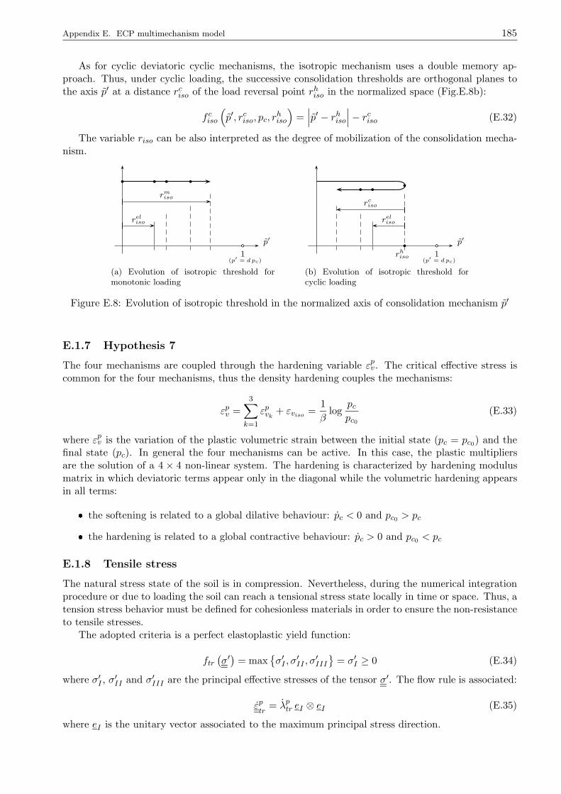
Appendix E. ECP multimechanism model 185
As for cyclic deviatoric cyclic mechanisms, the isotropic mechanism uses a double memory ap-proach. Thus, under cyclic loading, the successive consolidation thresholds are orthogonal planes tothe axis p′ at a distance rciso of the load reversal point rhiso in the normalized space (Fig.E.8b):
f ciso
(
p′, rciso, pc, rhiso
)
=∣∣∣p′ − rhiso
∣∣∣− rciso (E.32)
The variable riso can be also interpreted as the degree of mobilization of the consolidation mecha-nism.
p′
1(p′ = d pc)
reliso
rmiso
b b b b
(a) Evolution of isotropic threshold formonotonic loading
p′
1(p′ = d pc)
reliso
rciso
b bb
b
rhiso
(b) Evolution of isotropic threshold forcyclic loading
Figure E.8: Evolution of isotropic threshold in the normalized axis of consolidation mechanism p′
E.1.7 Hypothesis 7
The four mechanisms are coupled through the hardening variable εpv. The critical effective stress iscommon for the four mechanisms, thus the density hardening couples the mechanisms:
εpv =
3∑
k=1
εpvk+ εviso
=1
βlog
pcpc0
(E.33)
where εpv is the variation of the plastic volumetric strain between the initial state (pc = pc0) and thefinal state (pc). In general the four mechanisms can be active. In this case, the plastic multipliersare the solution of a 4 × 4 non-linear system. The hardening is characterized by hardening modulusmatrix in which deviatoric terms appear only in the diagonal while the volumetric hardening appearsin all terms: the softening is related to a global dilative behaviour: pc < 0 and pc0 > pc the hardening is related to a global contractive behaviour: pc > 0 and pc0 < pc
E.1.8 Tensile stress
The natural stress state of the soil is in compression. Nevertheless, during the numerical integrationprocedure or due to loading the soil can reach a tensional stress state locally in time or space. Thus, atension stress behavior must be defined for cohesionless materials in order to ensure the non-resistanceto tensile stresses.
The adopted criteria is a perfect elastoplastic yield function:
ftr(σ′)
= maxσ′I , σ
′II , σ
′III
= σ′I ≥ 0 (E.34)
where σ′I , σ′II and σ′III are the principal effective stresses of the tensor σ′. The flow rule is associated:
εptr
= λptr eI ⊗ eI (E.35)
where eI is the unitary vector associated to the maximum principal stress direction.
186 E.2. Numerical integration
E.2 Numerical integration
As extensively described in the previous section, each mechanism has its own yielding function fj,flow rule Ψ
jand plastic multiplier λpj . The evolution of some hardening variables are specific to each
mechanism rj or common to the four mechanisms εpv. Thus, a non active mechanism can have evolutionof its hardening variables even if it is not active. The flow rule of each mechanism can be written ina general form:
εpj
= λpj Ψj
j = 1, 2, 3, iso (E.36)
where the volumetric part of the plastic strain is controlled by the dilatancy law:
εpvj= λpj Ψvj
(E.37)
The following relation is still valid, defining the conditions of plastic state for each mechanism:
λpj ≥ 0 ; fj(σ′, rj , ε
pv
)≤ 0 ; λpj fj
(σ′, rj , ε
pv
)= 0 (E.38)
The evolution of the hardening variables are given by their evolution laws:
rj = λpj Lrj (E.39)
and (E.37). The total increment of εpv is computed over the active mechanisms:
εpv =∑
i
εpvii ∈Mp
act (E.40)
where Mpact is the set of activated mechanisms. We make the difference between the set of potentially
active mechanism Mppact and the set of active mechanism Mp
act:
Mppact = a | fa = 0Mpact =
b ∈Mppact | λb > 0
(E.41)
In the case of multimechanism plasticity, the denomination of the total load is used if all themechanisms are active, the denomination of partial load is used when not all mechanisms are activatedand the denomination of elastic regime when no mechanisms are activated.
The total strain increment can be written in terms of the contribution of active mechanisms:
ε = εe +∑
b
εpb
b ∈Mpact (E.42)
The active plastic multipliers are the solution of the non-linear system obtained using the compat-ibility equations of the potentially active mechanism (fa = 0). We write for each potentially activemechanism a, keeping only the terms of the active mechanism b (λpb > 0):
∑
b
(
∂fa∂σ′
: C : Ψb− ∂rafa : Lraδab − ∂εp
vfa : Ψvb
)
λb =∂fa∂σ′
: C : ε (E.43)
Similarly to the previous constitutive models, an explicit integration approach with variable timestep is adopted to perform the numerical integration of the soil constitutive model. For a load steptn, the material state is characterized by the stress state σ′
nand the hardening internal variables
regrouped in the vector ηn. The goal is to compute the state of the material for the load step tn+1
characterized by σ′n+1
and ηn+1
due to a strain increment εn+1
. The strain increment is approximatedby the relation:
Appendix E. ECP multimechanism model 187
εn+1≈εn+1− ε
n
∆tn+1(E.44)
assumed to be constant during the interval ∆tn+1 = tn+1 − tn. The previous increment is calculatediteratively, thus for an iteration k the approximation of the increment becomes:
εk+1n+1≈εk+1n+1− ε
n
∆tn+1(E.45)
As high non-linearities can appear during the loading, the time step increment ∆tn+1 is subdividedinto a set of substeps δtm to improve the integration procedure:
∆tn+1 =∑
m
δtm (E.46)
If the set of variables defining the material state is denoted by E (E =
σ′n, η
n
), the initial values
for the iteration procedure is taken from the converged values of the previous load step: E0n+1 = En.
For a substep m associated to an iteration k of the load step n + 1, thus to a strain increment εkn+1
,
the set of variables defining the state of the material Emk
n+1 can be obtained according to:
fmk
j
(
σ′mk
n+1, ηm
k
n+1
)
≤ 0
δAmk
n+1 = Amk
n+1 −Am−1k
n+1 ∀ A ∈ E (E.47)
where:
∆Amk
n+1 =∑
m
δAmk
n+1 (E.48)
The total increment of the load step for the variables which describe the state of the material canbe computed according to:
∆σ′kn+1
=∑
m
C(
σ′mk
n+1
)
:
εkn+1−∑
j
∑
m
λpm
j Ψmk
j
∆ηkjn+1=
∑
m
λpm
j Lkηj∀ j ∈Mp
act (E.49)
in order to compute the updated state of the material for the iteration k:
Akn+1 = An + ∆Akn+1 (E.50)

188 E.2. Numerical integration
Appendix F
One-dimensional linear elastic groundresponse
The general solution of the equation of elastodynamics in time domain (1.34) can be obtained bydecomposition of the displacement field us into an irrotational field from a scalar potential φ and arotational field from a vectorial potential χ:
us = gradφ+ rotχ (F.1)
with divχ = 0. With this decomposition, the displacement field can be decoupled into two partialdifference equations:
φ =1
c2p
∂2φ
∂t2
χ =1
c2s
∂2χ
∂t2(F.2)
with the standard notation for the P-waves and S-waves wave propagation velocities. For a stationarymonochromatic wave of circular frequency ω, a general solution of F.2 is given by:
φ = Aeiωcp
(cpt−l.x)= Afp
χ = Beiωcs
(cst−l.x) = Bfs (F.3)
where l is the unit director vector if all of the components are real and l.B = 0. Replacing in (F.1)we obtain:
us = − iωAcp
fp l +iω
csfsB ⊗ l = Apfp l +
iω
csfsB ⊗ l (F.4)
The previous expressions show that for the P-waves the motion follows the direction of propagationand that for the S-waves the motion takes place in a plane orthogonal to this direction. In this plane,the S-waves can be decomposed into a SH and a SV component according to:
ASH =iω
cs
Bz√
l2x + l2y
ASV =iω
cs
lxBy − lyBx√
l2x + l2y
(F.5)
where ASH and ASV are the amplitudes of displacements of SH and SV waves. The general earth-quake wave propagation problem is tridimensional, but in earthquake engineering context (near to thesurface) the problem can be treated as bidimensional assuming that the waves propagates parallel to
190
a vertical plane (yz for instance), thus the motion is independent of the x coordinate. In this case,the general solution can be written as (lx = 0):
us = ASV fslzex + (Apfply +ASHfslz) ey + (Apfplz −ASHfsly) ez (F.6)
The previous expression shows that for plane waves, the motion following x is decoupled from themotion in the plane yz. The motion in this plane is governed by the P and S-waves. If the incidentfield is vertical (lx = ly = 0), the problems becomes one-dimensional and the displacement field canbe written as:
us = ASV fsex +ASHfsey +Apfpez (F.7)
h
zs
zb
Ais Ar
s
Aib
Arb
Soil
Bedrock
ρs, css
ρb, csb
Figure F.1: Homogenous elastic soil layer overlying a half-space bedrock
We consider now a homogenous elastic soil layer overlying a half-space elastic rock (Fig.F.1). Thehorizontal displacement following y due to a vertically incident SH-waves in each material can bewritten as:
us = Aiseiωcss
(css t+zs) +Arseiωcss
(css t−zs)
ub = Aibeiωcsb
(csbt+zb)
+Arbeiωcsb
(csbt−zb)
(F.8)
where the upperscript i and r refer to incident and reflected field, and the subscript s and b refer tosoil and bedrock. The free surface condition (σyz = 0) imposes that Ars = Ais = As. The compatibilityof displacement and continuity of shear stress at the soil-bedrock interface require that:
As
(
eiωcss
h − e−iωcss
h)
= Aib +Arb (F.9)
According to the definition of shear stress (τyz = µ∂u∂z
), the relation between the amplitudes canbe summarized as (Pecker, 1984; Kramer, 1996):
Aib =1
2As
[
(1 + α) eiωcss
h+ (1− α) e
− iωcss
]
Aib =1
2As
[
(1− α) eiωcss
h+ (1 + α) e
− iωcss
]
(F.10)
where α is the impedance ratio defined by
α =
√ρscss
ρbcsb
(F.11)
Defining the transfer function T (ω) as the ratio of the ground movement amplitude to a hypotheticoutcrop bedrock movement:
T (ω) =2As2Aib
=1
cos iωcssh+ iα sin iω
cssh
→ |T (ω)| = 1√
cos2 iωcssh+ α2 sin2 iω
cssh
(F.12)
Appendix G
Substructure SSI approximation infrequency domain
Starting from the definition of the complete system shown in Fig.G.1, Aubry and Clouteau. (1992)and Clouteau and Aubry (2003) developed an analytical formulation of the dynamic SSI phenomenon,based on the substructure technique. This approach was integrated in the numerical code MISS3D,performing SSI analysis in the linear elastic or viscoelastic domain. The physical domain is decomposedinto three subdomains: the unbounded soil denoted by Ωs, the bounded foundation denoted by Ωf
and the bounded structure Ωb. In comparison with the decomposition shown in Fig.1.1, there are twomain differences: the soil domain Ωs is unbounded and the superstructure is decomposed into a rigiddomain Ωf and a flexible domain Ωb. The interfaces are denoted respectively by Σbf and Σsf . Freefield conditions are assumed into the other part of their boundary Γs and Γb.
Ωs
Γs
Γ∞s
Ωb
ΓbΩf
Σbf
Σsf
ui
Figure G.1: Definition of the global system for substructure approach
The permanent displacements fields on Γs and Γb due to static loads (weight and dead and/or liveloads) are assumed to be known in the following. We keep the notation for the dynamic perturbationsfields due to dynamic loads us(x, t) and ub(x, t). In this case, they are assumed to be small enough tosatisfy linear elastic hypothesis around the equilibrated static state. The corresponding elastic stresstensors due to dynamic perturbation are denoted by σ
sand σ
b.
The seismic loading is taken into account defining an incident field ui inside Ωs, defined as thedisplacement field in the soil without superstructure and foundation due to seismic motion. Assumingsmall deformations, the displacements fields us and ui verify elastodynamic equations in the soil:
div σs(us) = ρsus ∀ x ∈ Ωs
div σs(ui) = ρsui ∀ x ∈ Ωs (G.1)
while ub satisfies elastodynamic equation in the superstructure domain:
192 G.1. Rigid foundation
div σb(ub) = ρbub ∀ x ∈ Ωb (G.2)
Assuming that no uplift appears between soil and foundation, and no loss of contact takes placebetween the structure and its foundation, the following kinematic conditions are verified over theinterfaces:
ub = uf ∀ x ∈ Σbf and us = uf ∀ x ∈ Σsf (G.3)
and continuity of traction over these interfaces. Free field conditions are also verified in Γs and Γb.
Due to linearity of equations (G.1) and (G.2) a Fourier transform can be applied to solve theproblem in the frequency domain. Thus, the superstructure field displacement verifies:
div σb(ub) + ρbω
2ub = 0 ∀ x ∈ Ωb (G.4)
Using the same definition for the set of kinematically acceptable fields of §1.2.4, the weak formu-lation can be written as:
∫
Ωb
σb(ub) : ε
b(wb) dV − ω2
∫
Ωb
ρbub.wb dV =
∫
Σbf
tb (ub) .wb dS (G.5)
Choosing a rigid body mode ψn
as kinematical acceptable field, the following equation is obtained:
− ω2
∫
Ωb
ρbub.ψn dV =
∫
Σbf
tb (ub) .ψn dS (G.6)
for each rigid body mode ψn. Previous expression takes into account the fact that rigid body modes
do not induce deformations.
G.1 Rigid foundation
Assuming a rigid foundation Ωf , the corresponding displacement field uf can be written in terms ofthe rigid body modes ψ
m(x):
uf (x, ω) =6∑
m=1
cm (ω)ψm
(x) ∀ x ∈ Ωf (G.7)
where the six rigid body modes are three translational and three rotational modes passing by the threeprincipal axis of the foundation. cm are the participation factors depending on the frequency. As thefoundation is rigid, the equilibrium in moments and forces in terms of test functions wf can be writtenas:
∫
Σsf
ts (us) .wf dS +
∫
Σbf
tb (ub) .wf dS − ω2
∫
Ωf
ρf uf .wf dV = 0 (G.8)
Similarly to (G.6), by choosing rigid body modes ψn
as kinematical acceptable field, the previousexpression becomes:
∫
Σsf
ts (us) .ψn dS +
∫
Σbf
tb (ub) .ψn dS − ω2
∫
Ωf
ρf uf .ψn dV = 0 (G.9)
for each rigid body mode ψn.
Appendix G. Substructure SSI approximation in frequency domain 193
G.2 Decomposition of the displacement in the superstructure
The displacement field in the superstructure ub can be decomposed in two modal basis: the rigid bodymodal basis uf due to rigid body modes of the foundation, and the flexible modal part ub0 of thestructure under fixed base condition:
ub = uf + ub0 ∀ x ∈ Ωb (G.10)
The flexible modal field ub0 can be expressed in terms of the natural fixed base modes φj:
ub0 (x, ω) =∑
j≥1
qj (ω)φj(x) ∀ x ∈ Ωb (G.11)
where qj are the frequency-dependent modal participation factors. Using decompositions (G.7 and(G.11), the total displacement field of the superstructure is given by:
ub (x, ω) =6∑
m=1
cm (ω)ψm
(x) +∑
j≥1
qj (ω)φj(x) ∀ x ∈ Ωb (G.12)
Introducing (G.12) in the variational formulation (G.6) and the equilibrium equation (G.9), weobtain:
∫
σsf
ts (us) .ψn dS = ω2
6∑
m=1
cm
∫
Ωf
ρfψm.ψn dV +
6∑
m=1
cm
∫
Ωb
ρbψm.ψn dV +∑
j≥1
qj
∫
Ωb
ρbφj.ψn dV
(G.13)As the previous expression is still valid for each rigid body mode ψ
n, it can be written in an
equivalent matrix form in frequency domain:
∫
Σsf
ts (us) .Ψ dS − ω2 ([Mf ] + [Mb] + [M∗b (ω)]) c = 0 (G.14)
where Ψ regroups the rigid body modes and c the participation factors. [Mf ] and [Mb] are the massmatrix of the foundation and the superstructure, respectively. Their components can be computed as:
[Mf ]mn =
∫
Ωf
ρf ψm.ψn dV
[Mb]mn =
∫
Ωb
ρb ψm.ψn dV
The third matrix in (G.14) represents the equivalent added structural mass matrix [M∗b ] due to
the vibration of the flexible superstructure. It can be deduced by replacing the expression of modeparticipation factors qj in frequency domain for the SSI case (assuming mass normalized modes:∫
Ωbρb φj .φj dV = 1):
∑
j≥1
qj
∫
Ωb
ρb φj.ψn dV =
6∑
m=1
cm
∑
j≥1
ω2
ω2j + 2iζjωωj − ω2
∫
Ωb
ρb ψm.φj dV
∫
Ωb
ρb φj .ψn dV
(G.15)
where ωj and ζj are the natural frequency and modal damping associated to fixed base mode j. Thus,each component of the [M∗
b ] matrix can be computed as:
[M∗b ]mn =
∑
j≥1
ω2
ω2j + 2iζjωωj − ω2
∫
Ωb
ρb ψm.φj dV
∫
Ωb
ρb φj.ψn dV (G.16)
194 G.3. Decomposition of the displacement in the soil
This matrix is complex and highly dependent on the frequency. When ω approaches a modalfrequency value ωj, this matrix is purely complex and acts as a dashpot pumping energy to resonancemodes. For ω > ωj this term is approximately a pure negative real reducing the effective mass of thesystem. For ω < ωj the matrix is real and positive and tends towards zero for very low frequency(static case).
G.3 Decomposition of the displacement in the soil
The kinematic continuity over the interface Σbf in frequency domain can be written as:
ud (x, ω) = uf (ω)− ui (x, ω) =6∑
m=1
cm (x, ω) ψm
(x)− ui (x, ω) ∀ x ∈ Σbf (G.17)
where ud is the displacement field due to total diffracted waves. This diffracted displacement field,can be decomposed as follows:
ud (x, ω) =
6∑
m=1
udm (x, ω) + ud0 (x, ω) ∀ x ∈ Σbf (G.18)
The displacement field ud0 is the displacement due to local diffraction of the incident wave field onthe foundation assumed fixed. It verifies the elastodynamics equation in the soil domain Ωs and freefield conditions at the boundary Γs:
divσs
(ud0) + ρsω2ud0 = 0 in Ωs
ts (ud0) = 0 on Γs
ud0 = ui on Σsf (G.19)
The second component udm corresponds to displacement due to radiation caused by a unitaryfoundation movement along the rigid base mode m. Each component m also verifies:
div σs(udm) + ρsω
2udm = 0 in Ωs
ts (udm) = 0 on Γs
udm = ψm
on Σsf (G.20)
Injecting decomposition (G.18) in (G.14) we obtain the general system of equations of soil-structureinteraction:
([Ks (ω)]− ω2 [Mf ] + [Mb] + [M∗
b (ω)])c = fs (G.21)
where [Ks] is the generalized dynamic impedance of the soil and fs is the vector of induced seismicforces introduced at the foundation level. Their components can be computed as:
[Ks]mn =
∫
Σsf
ts (udm) .ψndS
fsn = −∫
Σsf
ts (ui + ud0) .ψn dS
The resolution of the previous system for each frequency ω gives the frequency-dependent modalparticipation factors regrouped in vector c. These values allow to compute displacement fields in thesuperstructure, foundation and soil. Compared to standard fixe base analysis, the previous expressionincludes the soil stiffness associated to impedance [Ks] and the interface forces fs induced by the

Appendix G. Substructure SSI approximation in frequency domain 195
ground motion. Even if the solution procedure is straightforward, its direct application involvesassembling matrices and vectors depending on the solution of boundary value problems (G.19) and(G.20). Thus, the Boundary Element Method is particulary well suited to these fields. Details aboutthe numerical approximation of these equations in the case of layered half-spaces implanted in MISS3Dare beyond of the scope of this presentation and can be found in Clouteau and Aubry (2001, 2003);Clouteau (1990, 2000, 2003).

196 G.3. Decomposition of the displacement in the soil
Appendix H
Numerical simulation of laboratory soiltest using ECP multimechanism model
The purpose of this section is complete the information concerning the set of parameter used forthe ECP multimechanism model described in §1.3.4 used in each case. Several soil mechanics testare modelled in order to show both a global view of the response of the constitutive model and thecoherence of the set of parameters proposed to simulate the non-linear soil behaviour.
The purpose of this section is complete the information concerning the set of parameter used forthe ECP multimechanism model described in §1.3.4 used in each case. Several soil mechanics testare modelled in order to show both a global view of the response of the constitutive model and thecoherence of the set of parameters proposed to simulate the non-linear soil behaviour.
H.1 Toyoura sand, Dr = 38%
For this material, the simulated soil mechanics test concern both undrained monotonic triaxial testand cyclic shear test at different consolidation pressures p′0. The available curves provided by Ishihara(1993) for monotonic loading and by Iwasaki et al. (1978) and Yamashita et al. (2001) for cyclic loadinghave been used as reference response path. According with these work, the main characteristics of theToyoura sand are: d50 = 0.19 [mm] d10 = 0.12 [mm] Uc = 1.3 [mm] emin = 0.597 [mm] emax = 0.997 [mm] φ′pp =31° ψ =31°whit the standard notation for grain diameter characteristics d50, d10 and Uc, minimum and maximumvoid ratio emin and emax. φ
′pp is the perfect plasticity friction angle and ψ the dilatancy angle. These
values are used as starting data for identification parameter strategy proposed by Lopez-Caballero(2003), in order to define some key parameters of the model as the plastic compressibility modulus β.Other parameters related to hardening and threshold domain are obtained using reference curves.
The simulations conducted for monotonic test correspond to an initial relative density ofDr = 38%.Four initial confinement pressures p′0 (i.e. 0.1, 1, 2 and 3 [MPa]) are used for the triaxial undrainedtests. The simulation results are presented in both planes q − ε1 and q − p′. Figure H.1 show the
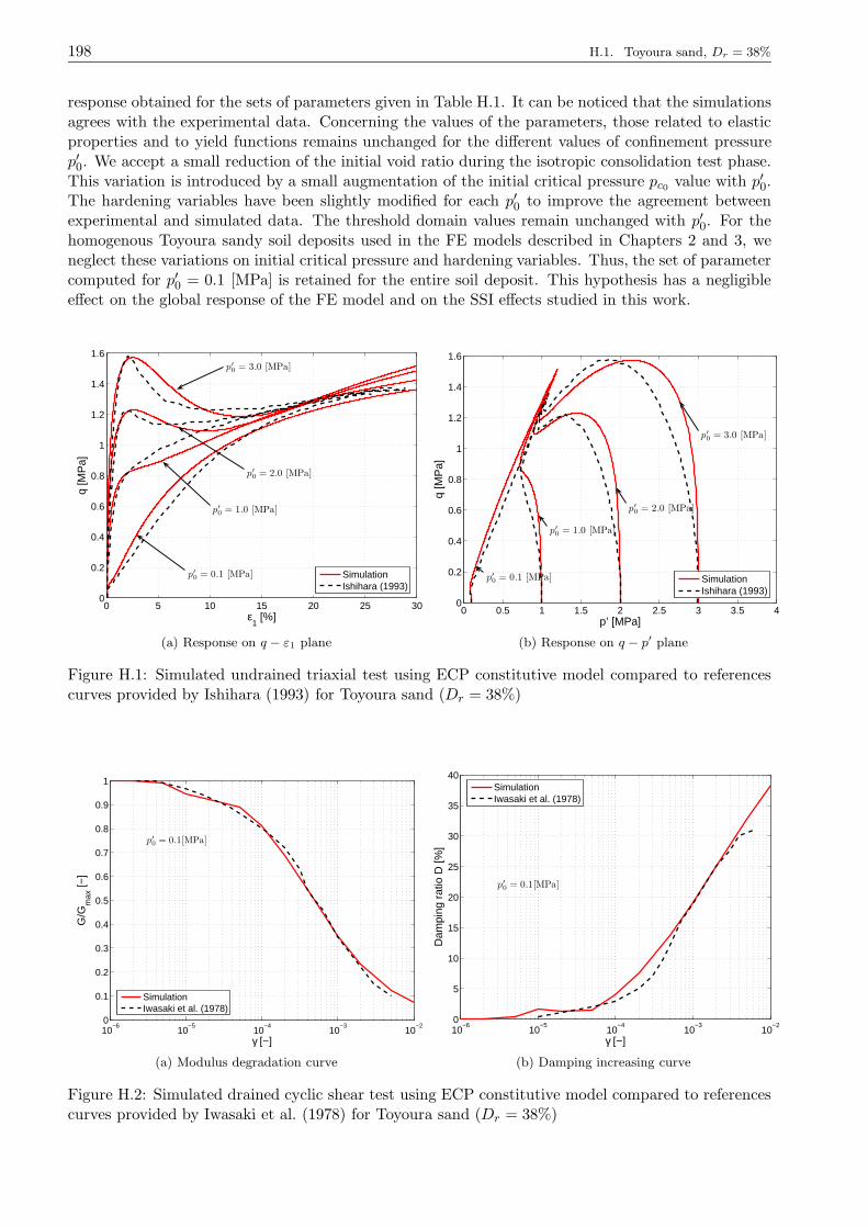
198 H.1. Toyoura sand, Dr = 38%
response obtained for the sets of parameters given in Table H.1. It can be noticed that the simulationsagrees with the experimental data. Concerning the values of the parameters, those related to elasticproperties and to yield functions remains unchanged for the different values of confinement pressurep′0. We accept a small reduction of the initial void ratio during the isotropic consolidation test phase.This variation is introduced by a small augmentation of the initial critical pressure pc0 value with p′0.The hardening variables have been slightly modified for each p′0 to improve the agreement betweenexperimental and simulated data. The threshold domain values remain unchanged with p′0. For thehomogenous Toyoura sandy soil deposits used in the FE models described in Chapters 2 and 3, weneglect these variations on initial critical pressure and hardening variables. Thus, the set of parametercomputed for p′0 = 0.1 [MPa] is retained for the entire soil deposit. This hypothesis has a negligibleeffect on the global response of the FE model and on the SSI effects studied in this work.
0 5 10 15 20 25 300
0.2
0.4
0.6
0.8
1
1.2
1.4
1.6
ε1 [%]
q [M
Pa]
SimulationIshihara (1993)
p′0
= 0.1 [MPa]
p′0
= 1.0 [MPa]
p′0
= 2.0 [MPa]
p′0
= 3.0 [MPa]
(a) Response on q − ε1 plane
0 0.5 1 1.5 2 2.5 3 3.5 40
0.2
0.4
0.6
0.8
1
1.2
1.4
1.6
p’ [MPa]
q [M
Pa]
SimulationIshihara (1993)
p′0
= 0.1 [MPa]
p′0
= 1.0 [MPa]
p′0
= 2.0 [MPa]
p′0
= 3.0 [MPa]
(b) Response on q − p′ plane
Figure H.1: Simulated undrained triaxial test using ECP constitutive model compared to referencescurves provided by Ishihara (1993) for Toyoura sand (Dr = 38%)
10−6
10−5
10−4
10−3
10−2
0
0.1
0.2
0.3
0.4
0.5
0.6
0.7
0.8
0.9
1
p′0
= 0.1[MPa]
γ [−]
G/G
max
[−]
SimulationIwasaki et al. (1978)
(a) Modulus degradation curve
10−6
10−5
10−4
10−3
10−2
0
5
10
15
20
25
30
35
40
p′0
= 0.1[MPa]
γ [−]
Dam
ping
rat
io D
[%]
SimulationIwasaki et al. (1978)
(b) Damping increasing curve
Figure H.2: Simulated drained cyclic shear test using ECP constitutive model compared to referencescurves provided by Iwasaki et al. (1978) for Toyoura sand (Dr = 38%)

Appendix H. Numerical simulation of laboratory soil test using ECP multimechanism model 199
In order to verify the model’s parameters under cyclic loading, the behaviour of the sand mustbe studied by simulating drained cyclic shear (DCS) tests. Fig.H.2 shows the responses of a DCStest obtained by the model of the Toyoura sand at a initial confinement of p′0 = 100[kPa]. The testresults are compared with the reference curves given by Iwasaki et al. (1978). We can notice that theobtained modulus degradation curve G
Gmax− γ curves match satisfactorily. The damping increasing
curve D − γ agrees with the experimental data for strains less than 0.5%, while for large strains thedamping is overestimated.
Table H.1: Parameters of ECP model for Toyoura sand, Dr = 38%
Dr [%] 38p′ [MPa] 0.1 1.0 2.0 3.0
Model parameters
Elasticity
Kref [MPa] 444 444 444 444Gref [MPa] 222 222 222 222
ne 0.4 0.4 0.4 0.4p′ref [MPa] 1.0 1.0 1.0 1.0
Yield function
φ′pp 31 31 31 31β 43 43 43 43d 3.5 3.5 3.5 3.5
b 0.2 0.2 0.2 0.2
Initial state
pc0 [MPa] 1.80 1.82 1.92 1.95pc0p′0
18 1.82 0.91 0.65
Hardening
a1 1× 10⁻⁴ 3× 10⁻⁴ 3× 10⁻⁴ 2× 10⁻³
a2 4× 10⁻³ 9× 10⁻³ 1.8× 10⁻² 2.3 × 10⁻²
cm 6× 10⁻² 6× 10⁻² 3× 10⁻² 1.8 × 10⁻²
cc 3× 10⁻² 3× 10⁻² 1.5× 10⁻² 9× 10⁻³
m 1.0 1.0 1.0 1.0np 1.0 1.0 1.0 1.0
Threshold domains
relk 5× 10⁻³ 5× 10⁻³ 5× 10⁻³ 5× 10⁻³
rhysk3× 10−2 3× 10⁻² 3× 10⁻² 3× 10⁻²
rmobk 8× 10⁻¹ 8× 10⁻¹ 8× 10⁻¹ 8× 10⁻¹
reliso 1× 10⁻³ 1× 10⁻³ 1× 10⁻³ 1× 10⁻³
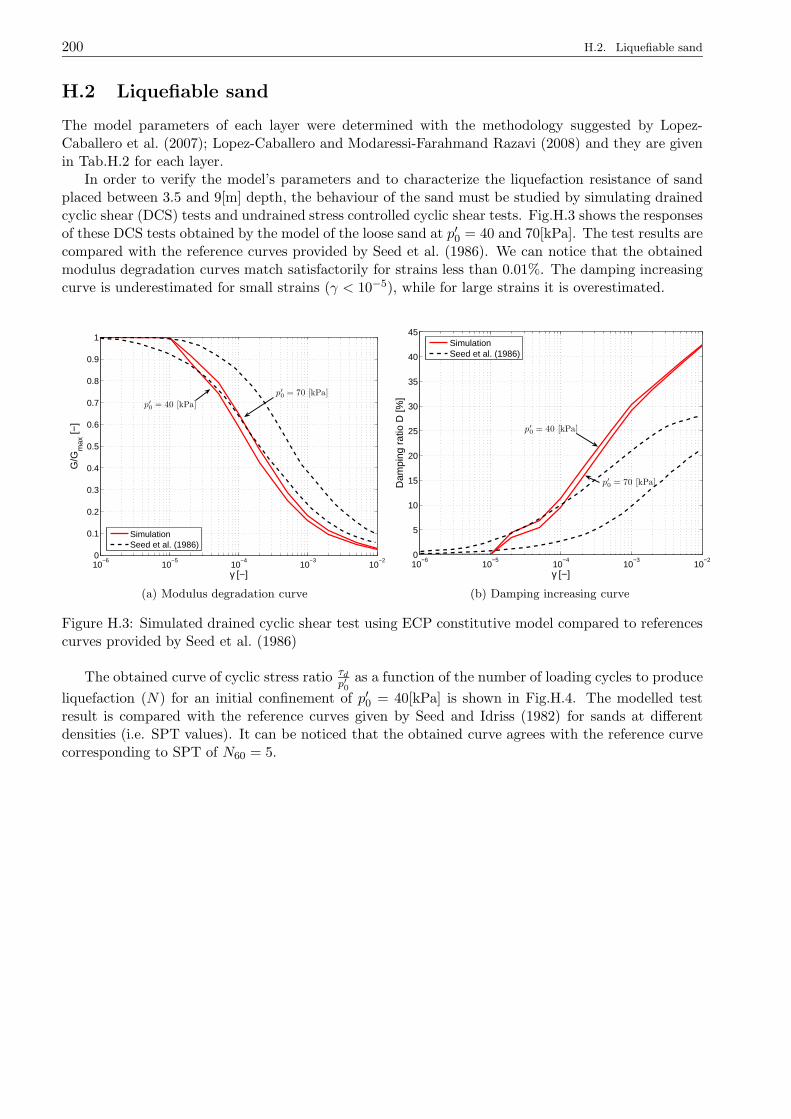
200 H.2. Liquefiable sand
H.2 Liquefiable sand
The model parameters of each layer were determined with the methodology suggested by Lopez-Caballero et al. (2007); Lopez-Caballero and Modaressi-Farahmand Razavi (2008) and they are givenin Tab.H.2 for each layer.
In order to verify the model’s parameters and to characterize the liquefaction resistance of sandplaced between 3.5 and 9[m] depth, the behaviour of the sand must be studied by simulating drainedcyclic shear (DCS) tests and undrained stress controlled cyclic shear tests. Fig.H.3 shows the responsesof these DCS tests obtained by the model of the loose sand at p′0 = 40 and 70[kPa]. The test results arecompared with the reference curves provided by Seed et al. (1986). We can notice that the obtainedmodulus degradation curves match satisfactorily for strains less than 0.01%. The damping increasingcurve is underestimated for small strains (γ < 10−5), while for large strains it is overestimated.
10−6
10−5
10−4
10−3
10−2
0
0.1
0.2
0.3
0.4
0.5
0.6
0.7
0.8
0.9
1
γ [−]
G/G
max
[−]
SimulationSeed et al. (1986)
p′0
= 40 [kPa]
p′0
= 70 [kPa]
(a) Modulus degradation curve
10−6
10−5
10−4
10−3
10−2
0
5
10
15
20
25
30
35
40
45
γ [−]
Dam
ping
rat
io D
[%]
SimulationSeed et al. (1986)
p′0
= 40 [kPa]
p′0
= 70 [kPa]
(b) Damping increasing curve
Figure H.3: Simulated drained cyclic shear test using ECP constitutive model compared to referencescurves provided by Seed et al. (1986)
The obtained curve of cyclic stress ratio τdp′0
as a function of the number of loading cycles to produce
liquefaction (N) for an initial confinement of p′0 = 40[kPa] is shown in Fig.H.4. The modelled testresult is compared with the reference curves given by Seed and Idriss (1982) for sands at differentdensities (i.e. SPT values). It can be noticed that the obtained curve agrees with the reference curvecorresponding to SPT of N60 = 5.

Appendix H. Numerical simulation of laboratory soil test using ECP multimechanism model 201
100
101
102
0.05
0.1
0.15
0.2
0.25
0.3
0.35
0.4
p′0
= 40[kPa]
N [−]
τ d / p 0’ [
−]
SimulationSeed and Idriss (1982)
N60 = 5
N60 = 10
Figure H.4: Comparison of simulated liquefaction curve with cyclic strength relations provided bySeed and Idriss (1982)
Table H.2: Parameters of ECP model for all soil profile layers
Layers 0− 2[m] 2− 9[m] 9− 16[m] 16− 22[m] 22− 29[m]
Model parameters
Permeability
ks [m/s] 1× 10⁻³ 1× 10⁻⁵ 1× 10⁻⁵ 1× 10⁻⁴ 1× 10⁻⁴
Elasticity
Kref [MPa] 90 628 628 628 444Gref [MPa] 45 290 290 290 22.4
ne 0.0 0.5 0.5 0.5 0.4p′ref [MPa] 1.0 1.0 1.0 1.0 1.0
Yield function
φ′pp° 31 30 30 30 31
β 20 33 33 33 43d 2.0 2.0 2.0 2.0 3.5b 0.2 0.2 0.2 0.2 0.2
Initial state
pc0 [MPa] 1.86 0.04 0.05 0.08 1.80
Hardening
ψ° 31 30 30 30 31a1 1× 10⁻⁴ 1× 10⁻⁴ 1× 10⁻⁴ 1× 10⁻⁴ 1× 10⁻⁴
a2 2× 10⁻⁴ 5× 10⁻³ 5× 10⁻³ 5× 10⁻³ 5× 10⁻³
cm 1× 10⁻³ 4× 10⁻³ 4× 10⁻³ 4× 10⁻³ 6× 10⁻²
cc 5× 10⁻⁴ 2× 10⁻³ 2× 10⁻³ 2× 10⁻³ 3× 10⁻²
m 1.0 1.5 1.5 1.5 1.0
Threshold domains
relk 1.3 × 10⁻² 3× 10⁻² 3× 10⁻² 3× 10⁻² 5× 10⁻³
rhysk2.2 × 10−1 4× 10⁻² 4× 10⁻² 4× 10⁻² 3× 10⁻²
rmobk 8× 10⁻¹ 8× 10⁻¹ 8× 10⁻¹ 8× 10⁻¹ 8× 10⁻¹
reliso 4× 10⁻³ 2× 10⁻² 2× 10⁻² 2× 10⁻² 1× 10⁻³
202 H.3. French Antilles soil
H.3 French Antilles soil
The model parameters of each layer were selected from the material library of ECP and are given inTab.H.3 for each layer. We use the same set of parameters for layers between 2 and 30[m] depth forthe sake of simplicity.
Table H.3: Parameters of ECP model for all soil profile layers
Layers 0− 2[m] 2− 6[m] 6− 10[m] 10− 20[m] 20− 30[m]
Model parameters
Elasticity
Kref [MPa] 90 399 399 399 399Gref [MPa] 45 184 184 184 184
ne 0.0 0.4 0.4 0.4 0.4p′ref [MPa] 1.0 1.0 1.0 1.0 1.0
Yield function
φ′pp° 31 33 33 33 33
β 20 17 17 17 17d 2.0 2.5 2.5 2.5 2.5b 0.2 0.2 0.2 0.2 0.2
Initial state
pc0 [MPa] 1.86 7.20 7.20 7.20 7.20
Hardening
ψ° 31 33 33 33 33a1 1× 10⁻⁴ 2× 10⁻⁴ 2× 10⁻⁴ 2× 10⁻⁴ 2× 10⁻⁴
a2 2.1× 10⁻⁴ 1.8× 10⁻² 1.8× 10⁻² 1.8× 10⁻² 1.8 × 10⁻²
cm 1× 10⁻³ 1× 10⁻⁴ 1× 10⁻⁴ 1× 10⁻⁴ 1× 10⁻⁴
cc 5× 10⁻⁴ 5× 10⁻⁵ 5× 10⁻⁵ 5× 10⁻⁵ 3× 10⁻⁵
m 1.0 1.0 1.0 1.0 1.0
Threshold domains
relk 1.3× 10⁻² 1× 10⁻² 1× 10⁻² 1× 10⁻² 1× 10⁻³
rhysk2.2× 10−1 5× 10⁻² 5× 10⁻² 5× 10⁻² 5× 10⁻²
rmobk 8× 10⁻¹ 9× 10⁻¹ 9× 10⁻¹ 9× 10⁻¹ 9× 10⁻¹
reliso 4× 10⁻³ 1× 10⁻⁴ 1× 10⁻⁴ 1× 10⁻⁴ 1× 10⁻⁴
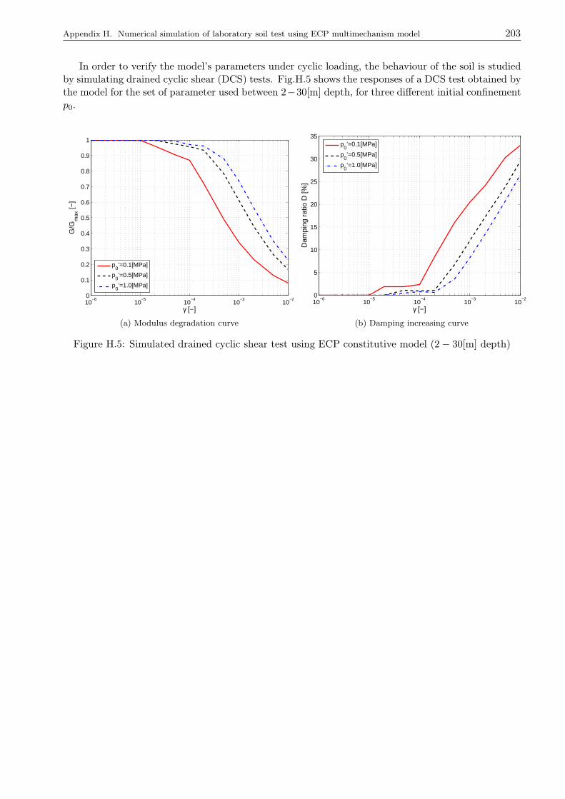
Appendix H. Numerical simulation of laboratory soil test using ECP multimechanism model 203
In order to verify the model’s parameters under cyclic loading, the behaviour of the soil is studiedby simulating drained cyclic shear (DCS) tests. Fig.H.5 shows the responses of a DCS test obtained bythe model for the set of parameter used between 2−30[m] depth, for three different initial confinementp0.
10−6
10−5
10−4
10−3
10−2
0
0.1
0.2
0.3
0.4
0.5
0.6
0.7
0.8
0.9
1
γ [−]
G/G
max
[−]
p0’=0.1[MPa]
p0’=0.5[MPa]
p0’=1.0[MPa]
(a) Modulus degradation curve
10−6
10−5
10−4
10−3
10−2
0
5
10
15
20
25
30
35
γ [−]D
ampi
ng r
atio
D [%
]
p0’=0.1[MPa]
p0’=0.5[MPa]
p0’=1.0[MPa]
(b) Damping increasing curve
Figure H.5: Simulated drained cyclic shear test using ECP constitutive model (2− 30[m] depth)

204 H.3. French Antilles soil

Appendix I
Description of studied buildings
This appendix gives additional details concerning buildings studied in this work. General geometryand reinforcement description are provided with the degree of detail required to be used in plastic-hinge beam column elements of GEFDyn . Additional details concerning reinforcement diameters andtransversal reinforcement dispositions are omitted here for sake of simplicity.
I.1 Two-level building: b01
I.1.1 Geometry
The two-level b01 building extracted from Marante et al. (2005) corresponds to an adaption of atrue-scale model performed by Vecchio and Emara (1992). The general geometry, label identificationof sections and a schema of transversal properties required for plastic-hinge elements are shown inFigI.1.
C1
C1
C1
C1
B1
B1
4[m]
2.2
[m]
2.0
[m]
bs
h ds
dc
Acs
As
typicaltransverse
section
Figure I.1: Geometry and transverse section descriptions of b01 building
I.1.2 Transverse sections
Table I.1 shows dimension of transverse sections, steel reinforcement area and unitary mass ρ. Thisunitary mass takes into account the self weight of the frame and the tributary weight/loading across laaccording to Fig.3.2. Last value is used to compute body forces due to gravity for static initializationanalysis and assemble the mass matrices for dynamic computations.
Table I.1: Transverse section properties
Label h[m] bs[m] dc[m] ds[m] As[cm2] Acs[cm2] ρ[kg/m3]
B1 0.4 0.3 0.03 0.37 11.4 11.4 42473
C1 0.4 0.4 0.02 0.38 11.4 11.4 -

206 I.1. Two-level building: b01
I.1.3 Materials
Numerical values of different mechanical properties are indicated in Tab.I.2, extracted from Maranteet al. (2005).
Table I.2: Mechanical properties of material for b01 building
Mechanical property Symbol Value
Resistance tocompressive stresses
fc 30[MPa]
Yield stress of steel fy 418[MPa]
Ultimate stress of steel fsu596[MPa]
Elastic modulus of steel Es 210[GPa]
Elastic modulus ofconcrete
Ec 26.5[GPa]
Crushing strain ofconcrete
εc 0.0034
I.1.4 Axial load-moment interaction diagrams
Figure I.2 displays axial force-moment interaction diagrams that control non-linear behavior of plastic-hinge beam elements of b01 building, computed using a resistance factor of φ = 0.9. It can be noticedthat no interaction is supposed for beams B1, thus plastic hinge apparition depends only on thebending moments for these elements.
−1.5 −1 −0.5 0 0.5 1 1.5
x 105
−1
−0.8
−0.6
−0.4
−0.2
0
0.2
0.4
0.6
0.8
1x 10
10
Moment [Nm]
Axi
al F
orce
[N]
(a) Beams (B1)
−3 −2 −1 0 1 2 3
x 105
−1
−0.5
0
0.5
1
1.5
2
2.5
3
3.5
4x 10
6
Moment [Nm]
Axi
al F
orce
[N]
(b) Columns (C1)
Figure I.2: Axial force-moment interaction diagrams used for plastic-hinge beam-column elements ofb01 building

Appendix I. Description of studied buildings 207
I.2 Seven-level building: b02
I.2.1 Geometry
The seven-level b02 building extracted from Marante et al. (2005) corresponds to a residential buildingplaced in Merida city, Venezuela. This building was designed according to seismic recommendationsof this country. The general geometry, label identification of sections and a schema of transversalproperties required for plastic-hinge elements are shown in Fig.I.3.
C1C2 C2
C2
C2
C3
C4
C4
C4
C4 C4
C4 C4
C5 C5
C5 C5
C5 C5
C5 C5
C5
B1 B1
B1 B1
B1 B1
B1 B1
B1 B1
B1 B1
B2 B2
B3 B3
4[m] 4[m]
2.6
[m]
2.6
[m]
2.6
[m]
2.6
[m]
2.6
[m]
2.6
[m]
2.6
[m]
1.9
2[m
]
b
h d
dc
Acs
As
typicaltransverse
section
Figure I.3: Geometry and transverse section descriptions of b02 building
I.2.2 Transverse sections
Table I.3 shows dimensions of transverse sections, steel reinforcement area and unitary mass ρ. Thisunitary mass takes into account the self weight of the frame and the tributary weight/loading across laaccording to Fig.3.2. Last value is used to compute body forces due to gravity for static initializationanalysis and assemble the mass matrices for dynamic computations.
I.2.3 Materials
Numerical values of different mechanical properties are indicated in Tab.I.4, extracted from Maranteet al. (2005).
I.2.4 Axial load-moment interaction diagrams
Figure I.4 displays axial force-moment interaction diagrams that control non-linear behavior of plastic-hinge beam elements of b02 building, computed using a resistance factor of φ = 0.9. It can be noticedthat no interaction is supposed for beams, thus plastic hinge apparition depends only on the bendingmoments of these elements.
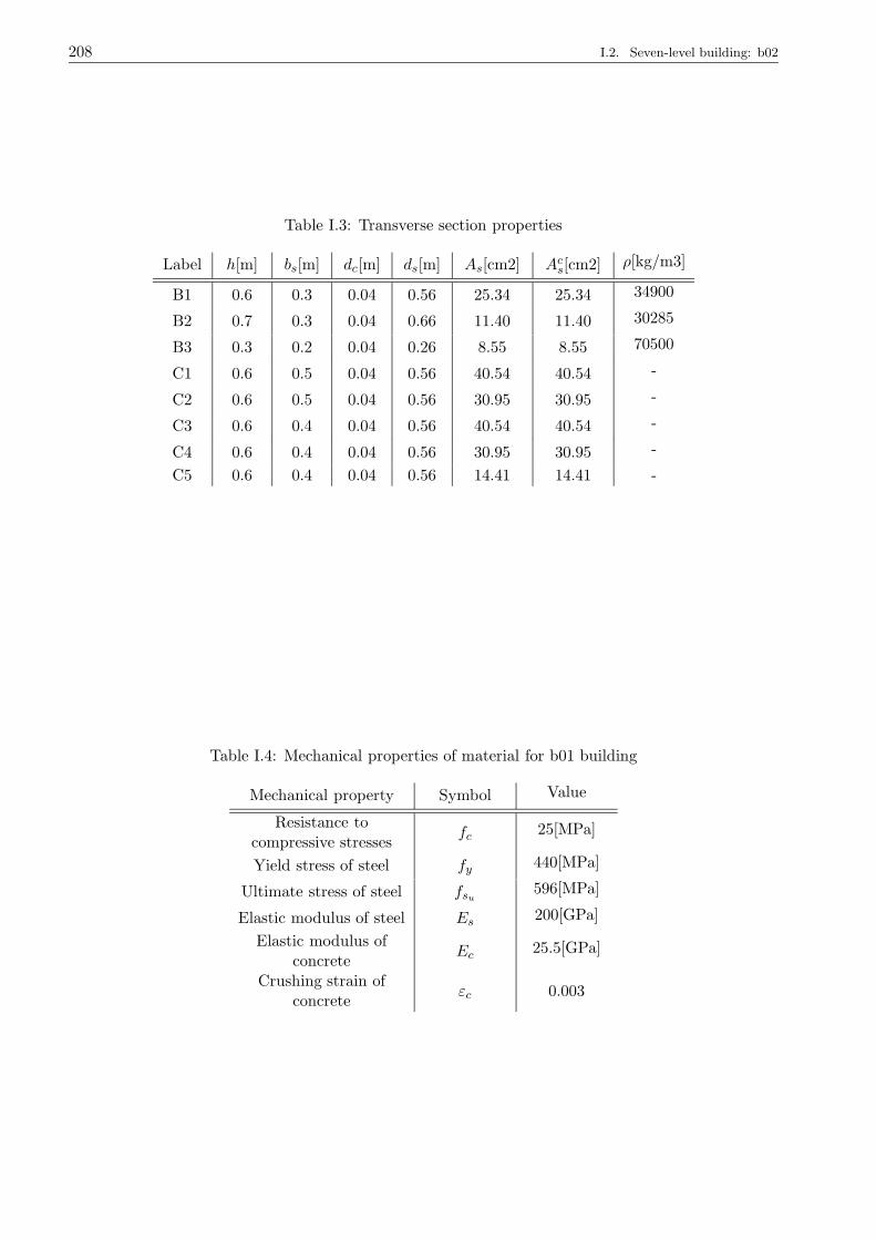
208 I.2. Seven-level building: b02
Table I.3: Transverse section properties
Label h[m] bs[m] dc[m] ds[m] As[cm2] Acs[cm2] ρ[kg/m3]
B1 0.6 0.3 0.04 0.56 25.34 25.34 34900
B2 0.7 0.3 0.04 0.66 11.40 11.40 30285
B3 0.3 0.2 0.04 0.26 8.55 8.55 70500
C1 0.6 0.5 0.04 0.56 40.54 40.54 -
C2 0.6 0.5 0.04 0.56 30.95 30.95 -
C3 0.6 0.4 0.04 0.56 40.54 40.54 -
C4 0.6 0.4 0.04 0.56 30.95 30.95 -
C5 0.6 0.4 0.04 0.56 14.41 14.41 -
Table I.4: Mechanical properties of material for b01 building
Mechanical property Symbol Value
Resistance tocompressive stresses
fc 25[MPa]
Yield stress of steel fy 440[MPa]
Ultimate stress of steel fsu596[MPa]
Elastic modulus of steel Es 200[GPa]
Elastic modulus ofconcrete
Ec 25.5[GPa]
Crushing strain ofconcrete
εc 0.003
Appendix I. Description of studied buildings 209
−6 −4 −2 0 2 4 6
x 105
−1
−0.8
−0.6
−0.4
−0.2
0
0.2
0.4
0.6
0.8
1x 10
10
Moment [Nm]
Axi
al F
orce
[N]
(a) Beams B1
−3 −2 −1 0 1 2 3
x 105
−1
−0.8
−0.6
−0.4
−0.2
0
0.2
0.4
0.6
0.8
1x 10
10
Moment [Nm]
Axi
al F
orce
[N]
(b) Beams B2
−8 −6 −4 −2 0 2 4 6 8
x 104
−1
−0.8
−0.6
−0.4
−0.2
0
0.2
0.4
0.6
0.8
1x 10
10
Moment [Nm]
Axi
al F
orce
[N]
(c) Beams B3
−1.5 −1 −0.5 0 0.5 1 1.5
x 106
−4
−2
0
2
4
6
8
10x 10
6
Moment [Nm]
Axi
al F
orce
[N]
(d) Columns C1
−1.5 −1 −0.5 0 0.5 1 1.5
x 106
−4
−2
0
2
4
6
8
10x 10
6
Moment [Nm]
Axi
al F
orce
[N]
(e) Columns C2
−1.5 −1 −0.5 0 0.5 1 1.5
x 106
−4
−2
0
2
4
6
8x 10
6
Moment [Nm]
Axi
al F
orce
[N]
(f) Columns C3
−1 −0.5 0 0.5 1
x 106
−3
−2
−1
0
1
2
3
4
5
6
7x 10
6
Moment [Nm]
Axi
al F
orce
[N]
(g) Columns C4
−6 −4 −2 0 2 4 6
x 105
−2
−1
0
1
2
3
4
5
6x 10
6
Moment [Nm]
Axi
al F
orce
[N]
(h) Columns C5
Figure I.4: Axial force-moment interaction diagrams used for plastic-hinge beam-column elements ofb02 building
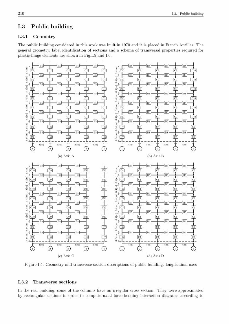
210 I.3. Public building
I.3 Public building
I.3.1 Geometry
The public building considered in this work was built in 1970 and it is placed in French Antilles. Thegeneral geometry, label identification of sections and a schema of transversal properties required forplastic-hinge elements are shown in Fig.I.5 and I.6.
1 2 3 4 5
C6 C6 C6 C6
C6 C6 C6 C6
C1 C1 C1 C1
C1 C1 C1 C1
C1 C1 C1 C1
C1 C1 C1 C1
C1 C1 C1 C1
C7
C7
C2
C2
C2
C2
C2
C2 C2 C2 C2C4
B5 B5 B5 B5
B5 B5 B5 B5
B5 B5 B5 B5
B5 B5 B5 B5
B5 B5 B5 B5
B5 B5 B5 B5
B5 B5 B5 B5
B5 B5 B5 B5
4[m] 4[m] 4[m] 4[m]
3.4
[m]
3.4
[m]
3.4
[m]
3.4
[m]
3.4
[m]
3.4
[m]
3.3
4[m
]3.3
4[m
]
(a) Axis A
1 2 3 4 5
C6 C6 C6 C7
C6 C6 C6 C7
C9 C9 C9
C9 C9 C9
C9 C9 C9
C9 C9 C9
C9 C9 C9
C9 C9 C9
C7
C7
C10 C10
C10 C10
C10 C10
C10 C10
C10 C10
C10 C10C10C10
B8 B8 B8 B8
B8 B8 B5 B8
B8 B8 B5 B8
B8 B8 B5 B8
B8 B8 B5 B8
B8 B8 B5 B8
B8 B8 B5 B8
B8 B8 B5 B8
4[m] 4[m] 4[m] 4[m]
3.4
[m]
3.4
[m]
3.4
[m]
3.4
[m]
3.4
[m]
3.4
[m]
3.3
4[m
]3.3
4[m
]
(b) Axis B
1 2 3 4 5
C6 C6 C6 C7
C6 C6 C6 C7
C9 C9 C10 C10
C9 C9 C10 C10
C9 C9 C10 C10
C9 C9 C10 C10
C9 C9 C10 C10
C7
C7
C10
C10
C10
C10
C10
C10 C9 C9 C10 C10
B8 B8 B8
B8 B8 B8
B8 B8 B8
B8 B8 B8
B8 B8 B8
B8 B8 B8
B8 B8 B8
B8 B8 B8
4[m] 4[m] 4[m] 4[m]
3.4
[m]
3.4
[m]
3.4
[m]
3.4
[m]
3.4
[m]
3.4
[m]
3.3
4[m
]3.3
4[m
]
(c) Axis C
1 2 3 4 5
C1 C1 C1 C1
C1 C1 C1 C1
C1 C1 C1 C1
C1 C1 C1 C1
C1 C1 C1 C1
C1 C1 C1 C1
C1 C1 C1 C1
C3
C3
C3
C3
C3
C3
C3
C3 C2 C2 C2 C2C4
B5 B5 B5 B5
B5 B5 B5 B5
B5 B5 B5 B5
B5 B5 B5 B5
B5 B5 B5 B5
B5 B5 B5 B5
B5 B5 B5 B5
B5 B5 B5 B5
4[m] 4[m] 4[m] 4[m]
3.4
[m]
3.4
[m]
3.4
[m]
3.4
[m]
3.4
[m]
3.4
[m]
3.3
4[m
]3.3
4[m
]
(d) Axis D
Figure I.5: Geometry and transverse section descriptions of public building: longitudinal axes
I.3.2 Transverse sections
In the real building, some of the columns have an irregular cross section. They were approximatedby rectangular sections in order to compute axial force-bending interaction diagrams according to
Appendix I. Description of studied buildings 211
the geometry described in Fig.I.3. Table I.5 shows transverse sections properties: transverse areaA, transverse primary inertia I, factor α defining minor flexural properties (§D.2), reinforcementaccording and unitary mass ρ. This unitary mass takes into account the self weight of the frame anda part of the dead and live loads. Last value is used to compute body forces due to gravity for staticinitialization analysis and assemble the mass matrices for dynamic computations.
Table I.5: Transverse section properties
Label A[m2] I[m4] α h[m] bs[m] dc[m] ds[m] As[cm2] Acs[cm2] ρ[kg/m3]
C1 0.44 0.014 1.5 0.6 0.8 0.02 0.58 25.1 25.1 2400
C2 0.44 0.014 1.5 0.6 0.8 0.02 0.58 15.7 15.7 2400
C3 0.21 0.002 6.19 0.3 0.8 0.03 0.28 15.7 12.6 7000
C4 0.21 0.002 6.19 0.3 0.8 0.03 0.28 10.1 8.0 7000
B5 0.31 0.013 0.41 0.7 0.45 0.66 0.04 10.8 10.8 7000
C6 0.48 0.014 1.77 0.45 0.3 0.02 0.44 4.5 4.5 2400
C7 0.24 0.002 7.11 0.3 0.8 0.02 0.58 25.1 25.1 14000
B8 0.18 0.005 0.25 0.6 0.3 0.02 0.58 10.8 10.8 14000
C9 0.14 0.002 0.44 0.45 0.3 0.02 0.44 4.5 4.5 14000
C10 0.11 0.001 0.73 0.35 0.3 0.02 0.33 4.5 4.5 14000
B11 0.08 0.002 0.09 0.5 0.15 0.02 0.48 8.0 9.6 2400
B12 0.024 0.007 0.44 0.6 0.4 0.02 0.58 10.8 10.8 2400
I.3.3 Materials
Numerical values of different mechanical properties are indicated in Tab.I.6.
Table I.6: Mechanical properties of material for public building
Mechanical property Symbol Value
Resistance tocompressive stresses
fc 27.5[MPa]
Yield stress of steel fy 420[MPa]
Ultimate stress of steel fsu596[MPa]
Elastic modulus of steel Es 200[GPa]
Elastic modulus ofconcrete
Ec 24.8[GPa]
Crushing strain ofconcrete
εc 0.003
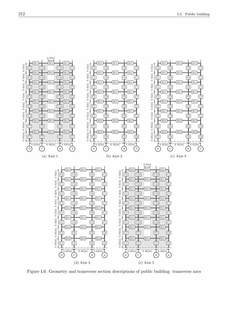
212 I.3. Public building
D C B A
C7 C7 C7
C7 C7 C7
C10 C10 C2
C10 C10 C2
C10 C10 C2
C10 C10 C2
C10 C10 C2
C7
C7
C3
C3
C3
C3
C3
C4 C10 C10 C4
B11 B11 B11
B11 B11 B11
B11 B11 B11
B11 B11 B11
B11 B11 B11
B11 B11 B11
B11 B11 B11
B11 B11 B11
4.42[m] 6.40[m] 4.42[m]
3.4
[m]
3.4
[m]
3.4
[m]
3.4
[m]
3.4
[m]
3.4
[m]
3.3
4[m
]3.3
4[m
]
2.2[m]
(a) Axis 1
D C B A
C6 C6 C6
C6 C6 C6
C9 C9 C1
C9 C9 C1
C9 C9 C1
C9 C9 C1
C9 C9 C1
C1
C1
C1
C1
C1
C1
C1
C2 C9 C9 C2
B12 B12 B12
B12 B12 B12
B11 B11 B11
B11 B11 B11
B11 B11 B11
B11 B11 B11
B11 B11 B11
B11 B11 B11
4.42[m] 6.40[m] 4.42[m]
3.4
[m]
3.4
[m]
3.4
[m]
3.4
[m]
3.4
[m]
3.4
[m]
3.3
4[m
]3.3
4[m
]
(b) Axis 2
D C B A
C6 C6 C6
C6 C6 C6
C9 C9 C1
C9 C9 C1
C9 C9 C1
C9 C9 C1
C9 C9 C1
C1
C1
C1
C1
C1
C1
C1
C2 C9 C9 C2
B12 B12 B12
B12 B12 B12
B11 B11 B11
B11 B11 B11
B11 B11 B11
B11 B11 B11
B11 B11 B11
B11 B11 B11
4.42[m] 6.40[m] 4.42[m]
3.4
[m]
3.4
[m]
3.4
[m]
3.4
[m]
3.4
[m]
3.4
[m]
3.3
4[m
]3.3
4[m
]
(c) Axis 3
D C B A
C6 C6 C6
C6 C6 C6
C10 C9 C1
C10 C9 C1
C10 C9 C1
C10 C9 C1
C10 C9 C1
C1
C1
C1
C1
C1
C1
C1
C2 C10 C9 C2
B12 B12 B12
B12 B12 B12
B11 B11 B11
B11 B11 B11
B11 B11 B11
B11 B11 B11
B11 B11 B11
B11 B11 B11
4.42[m] 6.40[m] 4.42[m]
3.4
[m]
3.4
[m]
3.4
[m]
3.4
[m]
3.4
[m]
3.4
[m]
3.3
4[m
]3.3
4[m
]
(d) Axis 4
D C B A
C7 C7 C6
C7 C7 C6
C10 C10 C1
C10 C10 C1
C10 C10 C1
C10 C10 C1
C10 C10 C1
C1
C1
C1
C1
C1
C1
C1
C2 C10 C10 C2
B11 B11 B11
B11 B11 B11
B11 B11 B11
B11 B11 B11
B11 B11 B11
B11 B11 B11
B11 B11 B11
B11 B11 B11
4.42[m] 6.40[m] 4.42[m]
3.4
[m]
3.4
[m]
3.4
[m]
3.4
[m]
3.4
[m]
3.4
[m]
3.3
4[m
]3.3
4[m
]
2.2[m]
(e) Axis 5
Figure I.6: Geometry and transverse section descriptions of public building: transverse axes
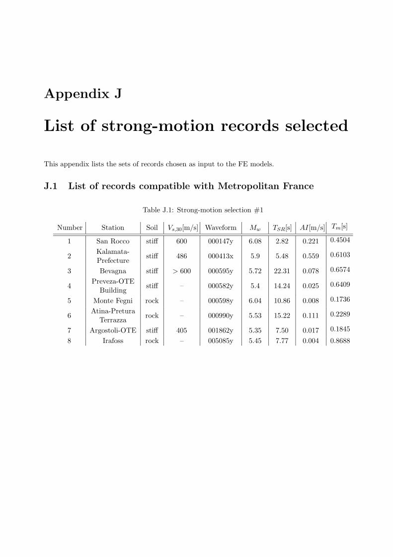
Appendix J
List of strong-motion records selected
This appendix lists the sets of records chosen as input to the FE models.
J.1 List of records compatible with Metropolitan France
Table J.1: Strong-motion selection #1
Number Station Soil Vs,30[m/s] Waveform Mw TSR[s] AI[m/s] Tm[s]
1 San Rocco stiff 600 000147y 6.08 2.82 0.221 0.4504
2Kalamata-Prefecture
stiff 486 000413x 5.9 5.48 0.559 0.6103
3 Bevagna stiff > 600 000595y 5.72 22.31 0.078 0.6574
4Preveza-OTE
Buildingstiff – 000582y 5.4 14.24 0.025 0.6409
5 Monte Fegni rock – 000598y 6.04 10.86 0.008 0.1736
6Atina-Pretura
Terrazzarock – 000990y 5.53 15.22 0.111 0.2289
7 Argostoli-OTE stiff 405 001862y 5.35 7.50 0.017 0.1845
8 Irafoss rock – 005085y 5.45 7.77 0.004 0.8688
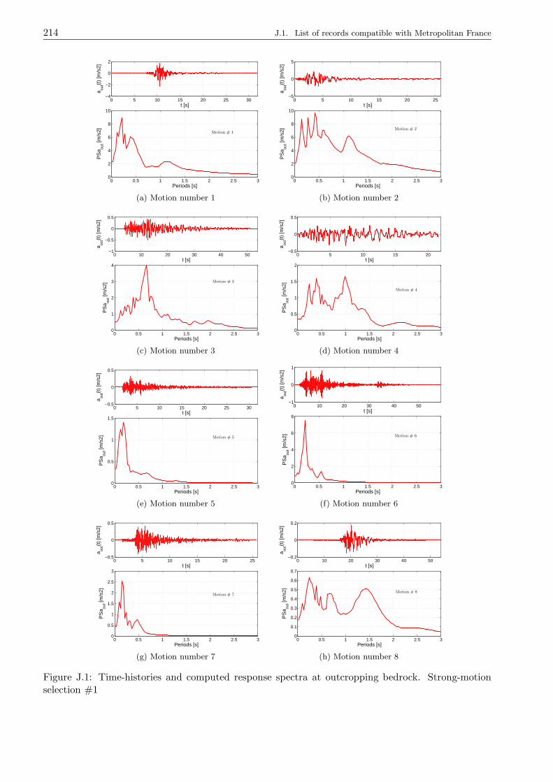
214 J.1. List of records compatible with Metropolitan France
0 5 10 15 20 25 30−4
−2
0
2
t [s]a ou
t(t)
[m/s
2]
0 0.5 1 1.5 2 2.5 30
2
4
6
8
10
Motion # 1
Periods [s]
PS
a out [m
/s2]
(a) Motion number 1
0 5 10 15 20 25−5
0
5
t [s]
a out(t
) [m
/s2]
0 0.5 1 1.5 2 2.5 30
2
4
6
8
10
Motion # 2
Periods [s]
PS
a out [m
/s2]
(b) Motion number 2
0 10 20 30 40 50−1
−0.5
0
0.5
t [s]
a out(t
) [m
/s2]
0 0.5 1 1.5 2 2.5 30
1
2
3
4
Motion # 3
Periods [s]
PS
a out [m
/s2]
(c) Motion number 3
0 5 10 15 20−0.5
0
0.5
t [s]
a out(t
) [m
/s2]
0 0.5 1 1.5 2 2.5 30
0.5
1
1.5
2
Motion # 4
Periods [s]
PS
a out [m
/s2]
(d) Motion number 4
0 5 10 15 20 25 30−0.5
0
0.5
t [s]
a out(t
) [m
/s2]
0 0.5 1 1.5 2 2.5 30
0.5
1
1.5
Motion # 5
Periods [s]
PS
a out [m
/s2]
(e) Motion number 5
0 10 20 30 40 50−1
0
1
t [s]
a out(t
) [m
/s2]
0 0.5 1 1.5 2 2.5 30
2
4
6
8
Motion # 6
Periods [s]
PS
a out [m
/s2]
(f) Motion number 6
0 5 10 15 20 25−0.5
0
0.5
t [s]
a out(t
) [m
/s2]
0 0.5 1 1.5 2 2.5 30
0.5
1
1.5
2
2.5
3
Motion # 7
Periods [s]
PS
a out [m
/s2]
(g) Motion number 7
0 10 20 30 40 50−0.2
0
0.2
t [s]
a out(t
) [m
/s2]
0 0.5 1 1.5 2 2.5 30
0.1
0.2
0.3
0.4
0.5
0.6
0.7
Motion # 8
Periods [s]
PS
a out [m
/s2]
(h) Motion number 8
Figure J.1: Time-histories and computed response spectra at outcropping bedrock. Strong-motionselection #1

Appendix J. List of strong-motion records selected 215
Table J.2: Strong-motion selection #2
Number Station Soil Vs,30[m/s] Waveform Mw TSR[s] AI[m/s] Tm[s]
9Forgaria-Cornio
stiff 441 000114x 5.33 4.25 0.044 0.2455
10 Cascia rock – 000242x 5.8 5.47 0.257 0.2393
11Valsamata-Seismograph
Stationrock – 000428y 5.3 15.16 0.251 0.2574
12 Bevagna stiff > 600 000595x 5.72 24.47 0.046 0.5572
13 San Rocco stiff 600 000147x 6.08 4.99 0.118 0.5198
14 Matelica stiff > 600 000601x 5.72 11.63 0.021 0.2114
15Cassino-Sant’Elia
alluvium – 000378x 5.9 12.74 0.202 0.5044
16ReykjavikHeidmork
rock – 005089x 5.45 8.16 0.004 0.8811
Table J.3: Strong-motion selection #3
Number Station Soil Vs,30[m/s] Waveform Mw TSR[s] AI[m/s] Tm[s]
17 Akhalkalaki rock – 000487x 5.48 8.83 0.007 0.2346
18Preveza-OTE
Buildingstiff – 000582x 5.4 16.43 0.022 0.5649
19 Villeta-Borrea rock – 000384x 5.53 3.64 0.132 0.1870
20Valsamata-Seismograph
rock – 000428x 5.3 15.78 0.138 0.2521
21Kalamata-Prefecture
stiff 486 000413y 5.9 7.04 0.841 0.5354
22 Bevagna stiff > 600 000596y 6 20.27 0.190 0.6177
23 Vasiliki-Town stiff 490 001990y 5.42 10.90 0.066 0.3877
24 Irafoss rock – 005085x 5.45 9.36 0.003 0.6974
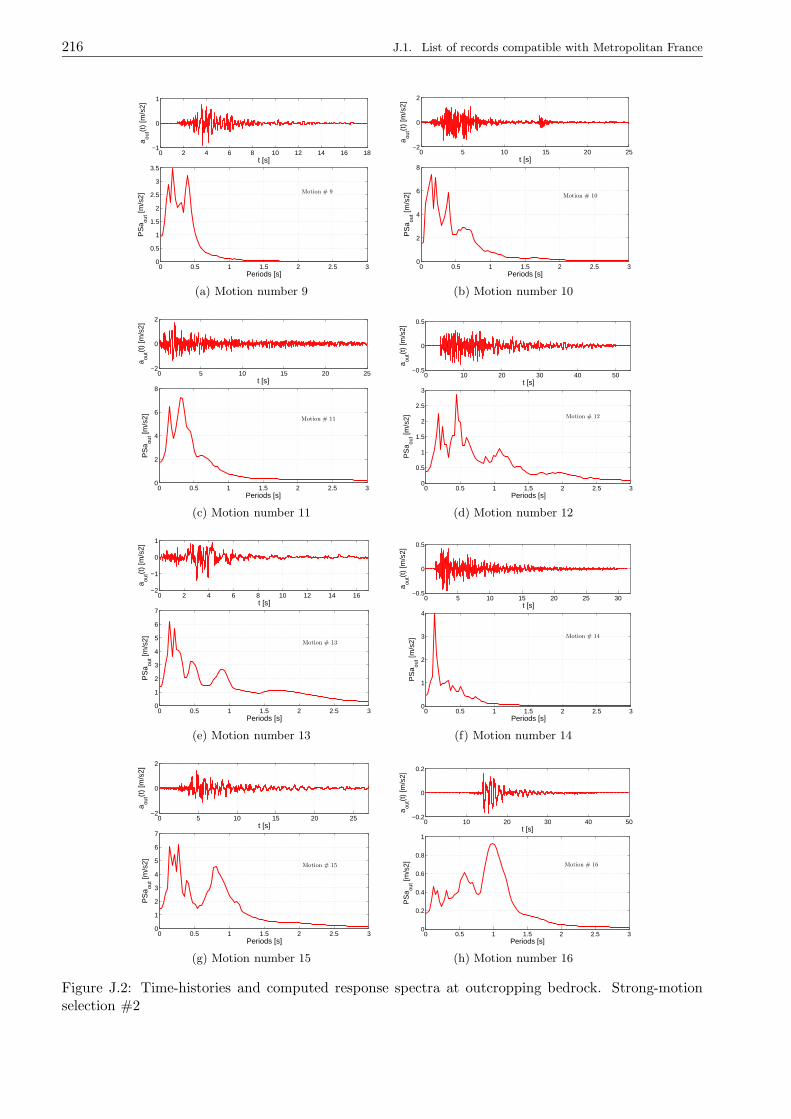
216 J.1. List of records compatible with Metropolitan France
0 2 4 6 8 10 12 14 16 18−1
0
1
t [s]
a out(t
) [m
/s2]
0 0.5 1 1.5 2 2.5 30
0.5
1
1.5
2
2.5
3
3.5
Motion # 9
Periods [s]
PS
a out [m
/s2]
(a) Motion number 9
0 5 10 15 20 25−2
0
2
t [s]
a out(t
) [m
/s2]
0 0.5 1 1.5 2 2.5 30
2
4
6
8
Motion # 10
Periods [s]
PS
a out [m
/s2]
(b) Motion number 10
0 5 10 15 20 25−2
0
2
t [s]
a out(t
) [m
/s2]
0 0.5 1 1.5 2 2.5 30
2
4
6
8
Motion # 11
Periods [s]
PS
a out [m
/s2]
(c) Motion number 11
0 10 20 30 40 50−0.5
0
0.5
t [s]
a out(t
) [m
/s2]
0 0.5 1 1.5 2 2.5 30
0.5
1
1.5
2
2.5
3
Motion # 12
Periods [s]
PS
a out [m
/s2]
(d) Motion number 12
0 2 4 6 8 10 12 14 16−2
−1
0
1
t [s]
a out(t
) [m
/s2]
0 0.5 1 1.5 2 2.5 30
1
2
3
4
5
6
7
Motion # 13
Periods [s]
PS
a out [m
/s2]
(e) Motion number 13
0 5 10 15 20 25 30−0.5
0
0.5
t [s]
a out(t
) [m
/s2]
0 0.5 1 1.5 2 2.5 30
1
2
3
4
Motion # 14
Periods [s]
PS
a out [m
/s2]
(f) Motion number 14
0 5 10 15 20 25−2
0
2
t [s]
a out(t
) [m
/s2]
0 0.5 1 1.5 2 2.5 30
1
2
3
4
5
6
7
Motion # 15
Periods [s]
PS
a out [m
/s2]
(g) Motion number 15
0 10 20 30 40 50−0.2
0
0.2
t [s]
a out(t
) [m
/s2]
0 0.5 1 1.5 2 2.5 30
0.2
0.4
0.6
0.8
1
Motion # 16
Periods [s]
PS
a out [m
/s2]
(h) Motion number 16
Figure J.2: Time-histories and computed response spectra at outcropping bedrock. Strong-motionselection #2
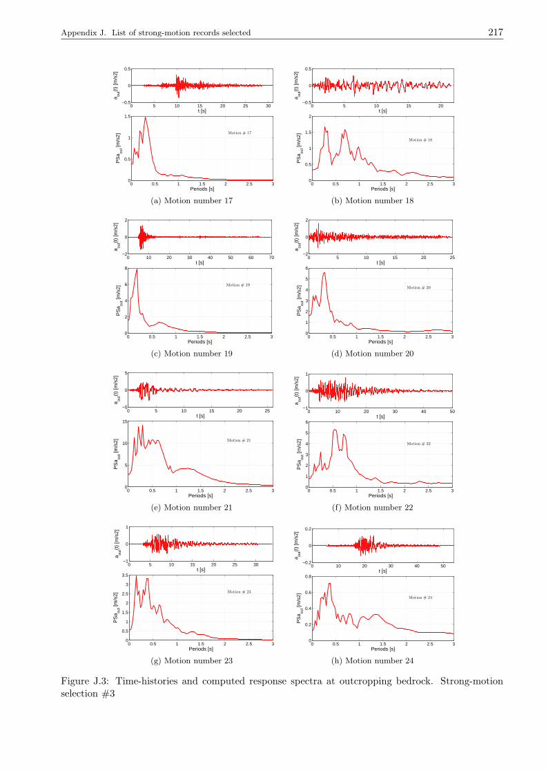
Appendix J. List of strong-motion records selected 217
0 5 10 15 20 25 30−0.5
0
0.5
t [s]a ou
t(t)
[m/s
2]
0 0.5 1 1.5 2 2.5 30
0.5
1
1.5
Motion # 17
Periods [s]
PS
a out [m
/s2]
(a) Motion number 17
0 5 10 15 20−0.5
0
0.5
t [s]
a out(t
) [m
/s2]
0 0.5 1 1.5 2 2.5 30
0.5
1
1.5
2
Motion # 18
Periods [s]
PS
a out [m
/s2]
(b) Motion number 18
0 10 20 30 40 50 60 70−2
0
2
t [s]
a out(t
) [m
/s2]
0 0.5 1 1.5 2 2.5 30
2
4
6
8
Motion # 19
Periods [s]
PS
a out [m
/s2]
(c) Motion number 19
0 5 10 15 20 25−2
0
2
t [s]
a out(t
) [m
/s2]
0 0.5 1 1.5 2 2.5 30
1
2
3
4
5
6
Motion # 20
Periods [s]
PS
a out [m
/s2]
(d) Motion number 20
0 5 10 15 20 25−5
0
5
t [s]
a out(t
) [m
/s2]
0 0.5 1 1.5 2 2.5 30
5
10
15
Motion # 21
Periods [s]
PS
a out [m
/s2]
(e) Motion number 21
0 10 20 30 40 50−1
0
1
t [s]
a out(t
) [m
/s2]
0 0.5 1 1.5 2 2.5 30
1
2
3
4
5
6
Motion # 22
Periods [s]
PS
a out [m
/s2]
(f) Motion number 22
0 5 10 15 20 25 30−1
0
1
t [s]
a out(t
) [m
/s2]
0 0.5 1 1.5 2 2.5 30
0.5
1
1.5
2
2.5
3
3.5
Motion # 23
Periods [s]
PS
a out [m
/s2]
(g) Motion number 23
0 10 20 30 40 50−0.2
0
0.2
t [s]
a out(t
) [m
/s2]
0 0.5 1 1.5 2 2.5 30
0.2
0.4
0.6
0.8
Motion # 24
Periods [s]
PS
a out [m
/s2]
(h) Motion number 24
Figure J.3: Time-histories and computed response spectra at outcropping bedrock. Strong-motionselection #3

218 J.1. List of records compatible with Metropolitan France
Table J.4: Strong-motion selection #4
Number Station Soil Vs,30[m/s] Waveform Mw TSR[s] AI[m/s] Tm[s]
25 Oseyrabru rock – 005090x 5.4 12.75 0.008 0.4806
26Athens-
Syntagmastiff 372 001713y 6.04 5.91 0.059 0.5443
27 Bevagna stiff > 600 000620y 5.5 19.31 0.046 0.5828
28Kalamata-
OTEBuilding
stiff 399 000414y 5.9 6.21 0.742 0.5251
29 Bevagna stiff > 600 000596x 6 21.61 0.146 0.6063
30Colfiorito-Casermette
rock – 000651x 5.58 5.42 0.209 0.2383
31Atina-Pretura
Terrazzarock – 000990x 5.53 10.21 0.145 0.2130
32KyparrisiaAgriculture
rock 862 001900x 5.36 5.00 0.016 0.2745
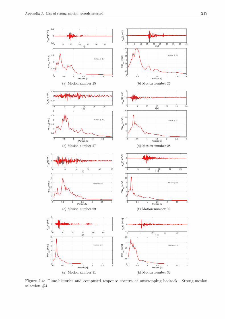
Appendix J. List of strong-motion records selected 219
0 10 20 30 40 50 60−0.5
0
0.5
t [s]a ou
t(t)
[m/s
2]
0 0.5 1 1.5 2 2.5 30
0.5
1
1.5
2
Motion # 25
Periods [s]
PS
a out [m
/s2]
(a) Motion number 25
0 5 10 15 20 25 30 35 40 45−1
0
1
t [s]
a out(t
) [m
/s2]
0 0.5 1 1.5 2 2.5 30
0.5
1
1.5
2
2.5
3
3.5
Motion # 26
Periods [s]
PS
a out [m
/s2]
(b) Motion number 26
0 5 10 15 20 25−1
−0.5
0
0.5
t [s]
a out(t
) [m
/s2]
0 0.5 1 1.5 2 2.5 30
0.5
1
1.5
2
2.5
3
Motion # 27
Periods [s]
PS
a out [m
/s2]
(c) Motion number 27
0 5 10 15 20 25 30−5
0
5
t [s]
a out(t
) [m
/s2]
0 0.5 1 1.5 2 2.5 30
5
10
15
20
Motion # 28
Periods [s]
PS
a out [m
/s2]
(d) Motion number 28
0 10 20 30 40 50−1
0
1
t [s]
a out(t
) [m
/s2]
0 0.5 1 1.5 2 2.5 30
1
2
3
4
5
6
Motion # 29
Periods [s]
PS
a out [m
/s2]
(e) Motion number 29
0 5 10 15 20 25−4
−2
0
2
t [s]
a out(t
) [m
/s2]
0 0.5 1 1.5 2 2.5 30
2
4
6
8
10
12
Motion # 30
Periods [s]
PS
a out [m
/s2]
(f) Motion number 30
0 10 20 30 40 50−2
0
2
t [s]
a out(t
) [m
/s2]
0 0.5 1 1.5 2 2.5 30
2
4
6
8
10
12
Motion # 31
Periods [s]
PS
a out [m
/s2]
(g) Motion number 31
0 5 10 15 20−1
0
1
t [s]
a out(t
) [m
/s2]
0 0.5 1 1.5 2 2.5 30
0.5
1
1.5
2
2.5
Motion # 32
Periods [s]
PS
a out [m
/s2]
(h) Motion number 32
Figure J.4: Time-histories and computed response spectra at outcropping bedrock. Strong-motionselection #4
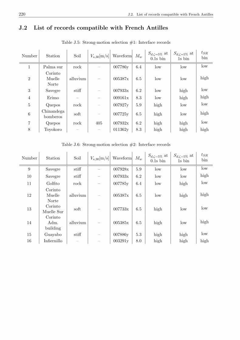
220 J.2. List of records compatible with French Antilles
J.2 List of records compatible with French Antilles
Table J.5: Strong-motion selection #1: Interface records
Number Station Soil Vs,30[m/s] Waveform MwSd,ζ=5% at0.1s bin
Sd,ζ=5% at1s bin
tSRbin
1 Palma sur rock – 007786y 6.4 low low low
2CorintoMuelleNorte
alluvium – 005387x 6.5 low low high
3 Savegre stiff – 007933x 6.2 low high low
4 Erimo – – 009161x 8.3 low high high
5 Quepos rock – 007927y 5.9 high low low
6Chinandegabomberos
soft – 007725y 6.5 high low high
7 Quepos rock 405 007932x 6.2 high high low
8 Toyokoro – – 011362y 8.3 high high high
Table J.6: Strong-motion selection #2: Interface records
Number Station Soil Vs,30[m/s] Waveform MwSd,ζ=5% at0.1s bin
Sd,ζ=5% at1s bin
tSRbin
9 Savegre stiff – 007928x 5.9 low low low
10 Savegre stiff – 007933x 6.2 low low high
11 Golfito rock – 007785y 6.4 low high low
12CorintoMuelleNorte
alluvium – 005387x 6.5 low high high
13Corinto
Muelle Sursoft – 007733x 6.5 high low low
14CorintoAdm.
buildingalluvium – 005385x 6.5 high low high
15 Guayabo stiff – 007886y 5.3 high high low
16 Infiernillo – – 003291y 8.0 high high high
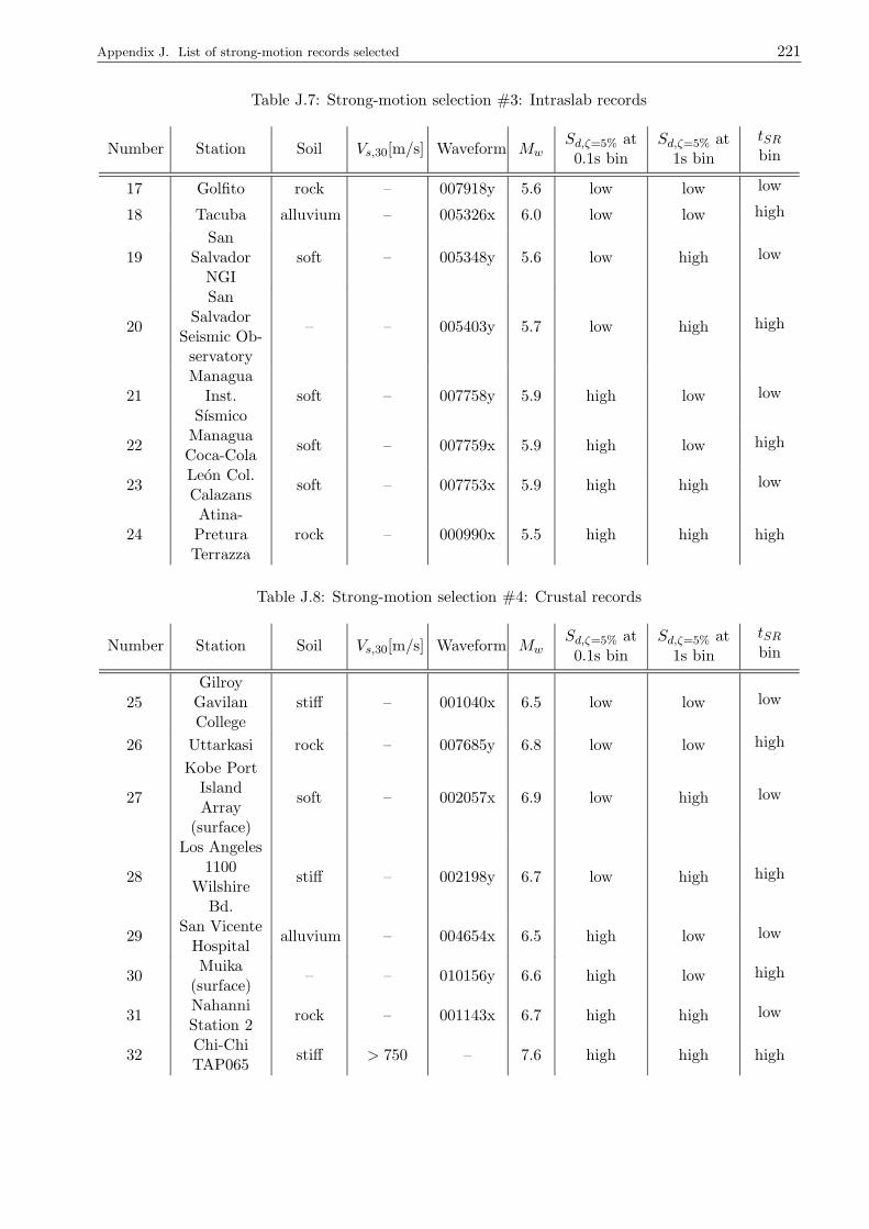
Appendix J. List of strong-motion records selected 221
Table J.7: Strong-motion selection #3: Intraslab records
Number Station Soil Vs,30[m/s] Waveform MwSd,ζ=5% at0.1s bin
Sd,ζ=5% at1s bin
tSRbin
17 Golfito rock – 007918y 5.6 low low low
18 Tacuba alluvium – 005326x 6.0 low low high
19San
SalvadorNGI
soft – 005348y 5.6 low high low
20
SanSalvador
Seismic Ob-servatory
– – 005403y 5.7 low high high
21Managua
Inst.Sısmico
soft – 007758y 5.9 high low low
22ManaguaCoca-Cola
soft – 007759x 5.9 high low high
23Leon Col.Calazans
soft – 007753x 5.9 high high low
24Atina-PreturaTerrazza
rock – 000990x 5.5 high high high
Table J.8: Strong-motion selection #4: Crustal records
Number Station Soil Vs,30[m/s] Waveform MwSd,ζ=5% at0.1s bin
Sd,ζ=5% at1s bin
tSRbin
25
GilroyGavilanCollege
stiff – 001040x 6.5 low low low
26 Uttarkasi rock – 007685y 6.8 low low high
27
Kobe PortIslandArray
(surface)
soft – 002057x 6.9 low high low
28
Los Angeles1100
WilshireBd.
stiff – 002198y 6.7 low high high
29San Vicente
Hospitalalluvium – 004654x 6.5 high low low
30Muika
(surface)– – 010156y 6.6 high low high
31NahanniStation 2
rock – 001143x 6.7 high high low
32Chi-ChiTAP065
stiff > 750 – 7.6 high high high
222 J.2. List of records compatible with French Antilles
Table J.9: Strong-motion selection #5: Crustal records
Number Station Soil Vs,30[m/s] Waveform MwSd,ζ=5% at0.1s bin
Sd,ζ=5% at1s bin
tSRbin
33 Hella stiff – 006330x 6.4 low low low
34
LosAngeles-
3620 SouthVermont
soft – 002664y 6.7 low low high
35San Jose
IBM Build.12
rock – 001043x 6.5 low high low
36BrawleyAirportHangar
soft – 001016y 6.5 low high high
37
SuperstitionMountainCameraSite 8
soft – 001109x 6.5 high low low
38Glendale3320 Las
Palmas Av.– – 002678y 6.7 high low high
39 Tsunan – – 008667y 6.6 high high low
40
El CentroArray
Station 6soft – 001022x 6.5 high high high
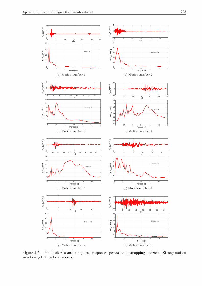
Appendix J. List of strong-motion records selected 223
0 50 100 150 200 250 300−2
0
2
4
t [s]a ou
t(t)
[m/s
2]
0 0.5 1 1.5 2 2.5 30
5
10
15
20
Motion # 1
Periods [s]
PS
a out [m
/s2]
(a) Motion number 1
0 10 20 30 40 50−1
0
1
t [s]
a out(t
) [m
/s2]
0 0.5 1 1.5 2 2.5 30
1
2
3
4
5
Motion # 2
Periods [s]
PS
a out [m
/s2]
(b) Motion number 2
0 2 4 6 8 10 12 14 16 18−5
0
5
t [s]
a out(t
) [m
/s2]
0 0.5 1 1.5 2 2.5 30
2
4
6
8
10
12
Motion # 3
Periods [s]
PS
a out [m
/s2]
(c) Motion number 3
0 10 20 30 40 50 60−0.5
0
0.5
t [s]
a out(t
) [m
/s2]
0 0.5 1 1.5 2 2.5 30.2
0.4
0.6
0.8
1
1.2
1.4
1.6
Motion # 4
Periods [s]
PS
a out [m
/s2]
(d) Motion number 4
0 10 20 30 40 50 60 70 80 90−5
0
5
t [s]
a out(t
) [m
/s2]
0 0.5 1 1.5 2 2.5 32
4
6
8
10
12
14
Motion # 5
Periods [s]
PS
a out [m
/s2]
(e) Motion number 5
0 5 10 15 20 25−2
0
2
t [s]
a out(t
) [m
/s2]
0 0.5 1 1.5 2 2.5 30
1
2
3
4
5
Motion # 6
Periods [s]
PS
a out [m
/s2]
(f) Motion number 6
0 5 10 15 20−5
0
5
t [s]
a out(t
) [m
/s2]
0 0.5 1 1.5 2 2.5 30
5
10
15
20
25
Motion # 7
Periods [s]
PS
a out [m
/s2]
(g) Motion number 7
0 5 10 15 20 25 30 35−0.5
0
0.5
t [s]
a out(t
) [m
/s2]
0 0.5 1 1.5 2 2.5 30
0.5
1
1.5
2
2.5
3
3.5
Motion # 8
Periods [s]
PS
a out [m
/s2]
(h) Motion number 8
Figure J.5: Time-histories and computed response spectra at outcropping bedrock. Strong-motionselection #1: Interface records
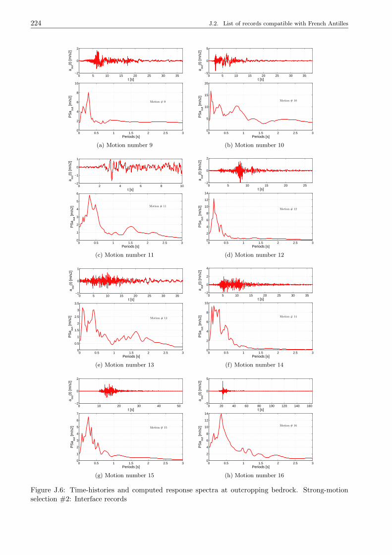
224 J.2. List of records compatible with French Antilles
0 5 10 15 20 25 30 35−2
0
2
t [s]
a out(t
) [m
/s2]
0 0.5 1 1.5 2 2.5 30
2
4
6
8
10
Motion # 9
Periods [s]
PS
a out [m
/s2]
(a) Motion number 9
0 5 10 15 20 25 30 35−5
0
5
t [s]
a out(t
) [m
/s2]
0 0.5 1 1.5 2 2.5 30
5
10
15
20
Motion # 10
Periods [s]
PS
a out [m
/s2]
(b) Motion number 10
0 2 4 6 8 10−2
−1
0
1
t [s]
a out(t
) [m
/s2]
0 0.5 1 1.5 2 2.5 30
1
2
3
4
5
6
Motion # 11
Periods [s]
PS
a out [m
/s2]
(c) Motion number 11
0 5 10 15 20 25−2
0
2
t [s]
a out(t
) [m
/s2]
0 0.5 1 1.5 2 2.5 30
2
4
6
8
10
12
14
Motion # 12
Periods [s]
PS
a out [m
/s2]
(d) Motion number 12
0 5 10 15 20 25 30 35−1
0
1
t [s]
a out(t
) [m
/s2]
0 0.5 1 1.5 2 2.5 30
0.5
1
1.5
2
2.5
3
3.5
Motion # 13
Periods [s]
PS
a out [m
/s2]
(e) Motion number 13
0 5 10 15 20 25 30 35−2
0
2
4
t [s]
a out(t
) [m
/s2]
0 0.5 1 1.5 2 2.5 30
2
4
6
8
10
Motion # 14
Periods [s]
PS
a out [m
/s2]
(f) Motion number 14
0 10 20 30 40 50−2
0
2
t [s]
a out(t
) [m
/s2]
0 0.5 1 1.5 2 2.5 30
1
2
3
4
5
6
7
Motion # 15
Periods [s]
PS
a out [m
/s2]
(g) Motion number 15
0 20 40 60 80 100 120 140 160−5
0
5
t [s]
a out(t
) [m
/s2]
0 0.5 1 1.5 2 2.5 30
2
4
6
8
10
12
14
Motion # 16
Periods [s]
PS
a out [m
/s2]
(h) Motion number 16
Figure J.6: Time-histories and computed response spectra at outcropping bedrock. Strong-motionselection #2: Interface records
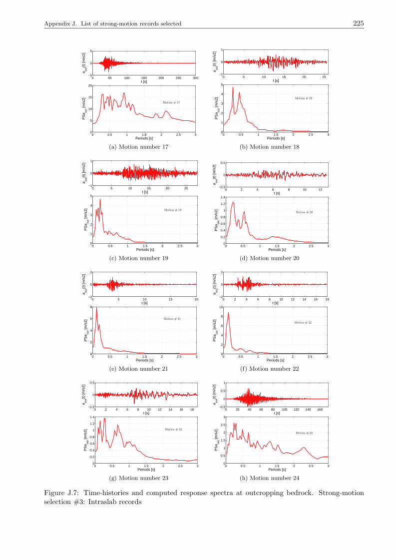
Appendix J. List of strong-motion records selected 225
0 50 100 150 200 250 300−5
0
5
t [s]a ou
t(t)
[m/s
2]
0 0.5 1 1.5 2 2.5 30
5
10
15
20
Motion # 17
Periods [s]
PS
a out [m
/s2]
(a) Motion number 17
0 5 10 15 20 25−1
0
1
t [s]
a out(t
) [m
/s2]
0 0.5 1 1.5 2 2.5 30
1
2
3
4
5
Motion # 18
Periods [s]
PS
a out [m
/s2]
(b) Motion number 18
0 5 10 15 20 25−1
0
1
t [s]
a out(t
) [m
/s2]
0 0.5 1 1.5 2 2.5 30
1
2
3
4
5
Motion # 19
Periods [s]
PS
a out [m
/s2]
(c) Motion number 19
0 2 4 6 8 10 12−0.5
0
0.5
t [s]
a out(t
) [m
/s2]
0 0.5 1 1.5 2 2.5 30
0.2
0.4
0.6
0.8
1
1.2
1.4
Motion # 20
Periods [s]
PS
a out [m
/s2]
(d) Motion number 20
0 5 10 15 20−2
0
2
t [s]
a out(t
) [m
/s2]
0 0.5 1 1.5 2 2.5 30
2
4
6
8
Motion # 21
Periods [s]
PS
a out [m
/s2]
(e) Motion number 21
0 2 4 6 8 10 12 14 16 18−2
0
2
t [s]
a out(t
) [m
/s2]
0 0.5 1 1.5 2 2.5 30
2
4
6
8
10
Motion # 22
Periods [s]
PS
a out [m
/s2]
(f) Motion number 22
0 2 4 6 8 10 12 14 16 18−0.5
0
0.5
t [s]
a out(t
) [m
/s2]
0 0.5 1 1.5 2 2.5 30
0.2
0.4
0.6
0.8
1
1.2
1.4
Motion # 23
Periods [s]
PS
a out [m
/s2]
(g) Motion number 23
0 20 40 60 80 100 120 140 160−0.5
0
0.5
1
t [s]
a out(t
) [m
/s2]
0 0.5 1 1.5 2 2.5 30
0.5
1
1.5
2
2.5
3
Motion # 24
Periods [s]
PS
a out [m
/s2]
(h) Motion number 24
Figure J.7: Time-histories and computed response spectra at outcropping bedrock. Strong-motionselection #3: Intraslab records
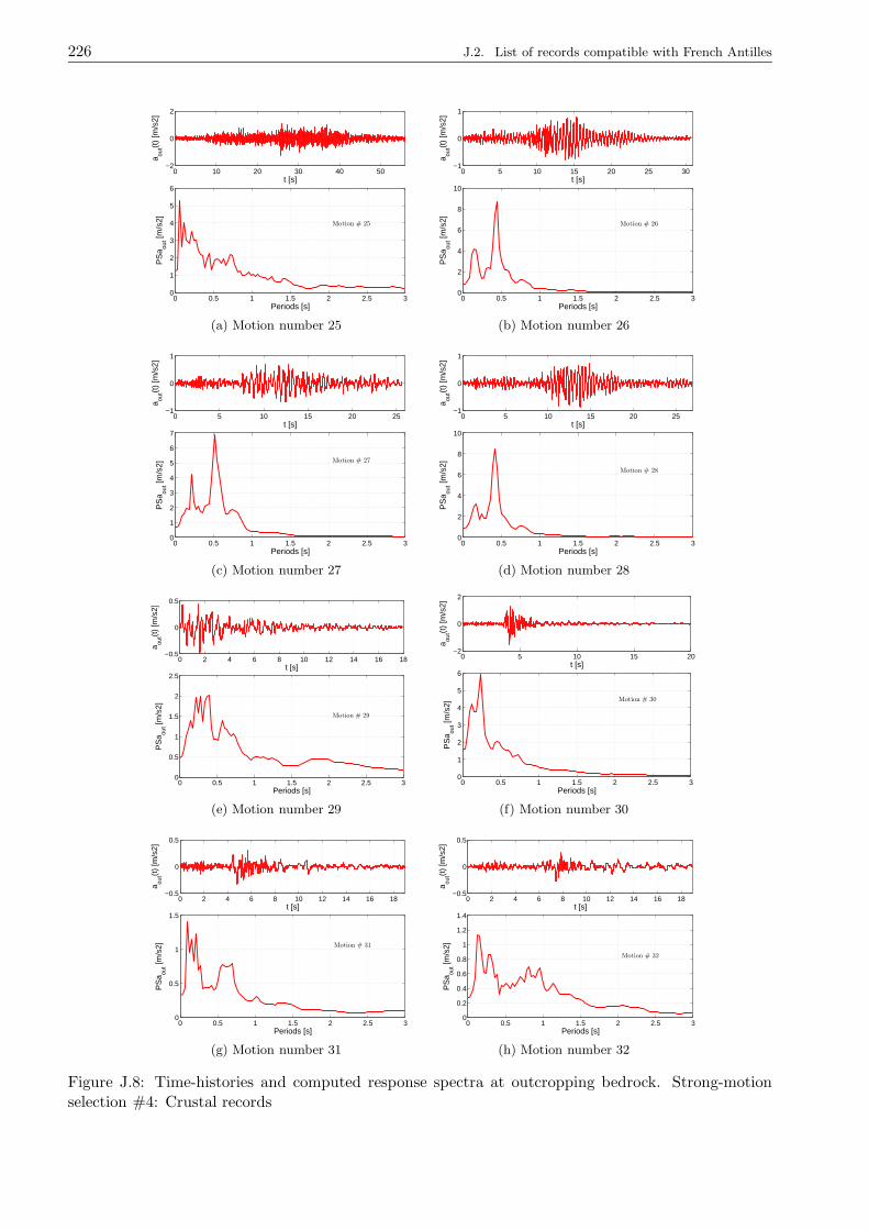
226 J.2. List of records compatible with French Antilles
0 10 20 30 40 50−2
0
2
t [s]
a out(t
) [m
/s2]
0 0.5 1 1.5 2 2.5 30
1
2
3
4
5
6
Motion # 25
Periods [s]
PS
a out [m
/s2]
(a) Motion number 25
0 5 10 15 20 25 30−1
0
1
t [s]
a out(t
) [m
/s2]
0 0.5 1 1.5 2 2.5 30
2
4
6
8
10
Motion # 26
Periods [s]
PS
a out [m
/s2]
(b) Motion number 26
0 5 10 15 20 25−1
0
1
t [s]
a out(t
) [m
/s2]
0 0.5 1 1.5 2 2.5 30
1
2
3
4
5
6
7
Motion # 27
Periods [s]
PS
a out [m
/s2]
(c) Motion number 27
0 5 10 15 20 25−1
0
1
t [s]
a out(t
) [m
/s2]
0 0.5 1 1.5 2 2.5 30
2
4
6
8
10
Motion # 28
Periods [s]
PS
a out [m
/s2]
(d) Motion number 28
0 2 4 6 8 10 12 14 16 18−0.5
0
0.5
t [s]
a out(t
) [m
/s2]
0 0.5 1 1.5 2 2.5 30
0.5
1
1.5
2
2.5
Motion # 29
Periods [s]
PS
a out [m
/s2]
(e) Motion number 29
0 5 10 15 20−2
0
2
t [s]
a out(t
) [m
/s2]
0 0.5 1 1.5 2 2.5 30
1
2
3
4
5
6
Motion # 30
Periods [s]
PS
a out [m
/s2]
(f) Motion number 30
0 2 4 6 8 10 12 14 16 18−0.5
0
0.5
t [s]
a out(t
) [m
/s2]
0 0.5 1 1.5 2 2.5 30
0.5
1
1.5
Motion # 31
Periods [s]
PS
a out [m
/s2]
(g) Motion number 31
0 2 4 6 8 10 12 14 16 18−0.5
0
0.5
t [s]
a out(t
) [m
/s2]
0 0.5 1 1.5 2 2.5 30
0.2
0.4
0.6
0.8
1
1.2
1.4
Motion # 32
Periods [s]
PS
a out [m
/s2]
(h) Motion number 32
Figure J.8: Time-histories and computed response spectra at outcropping bedrock. Strong-motionselection #4: Crustal records
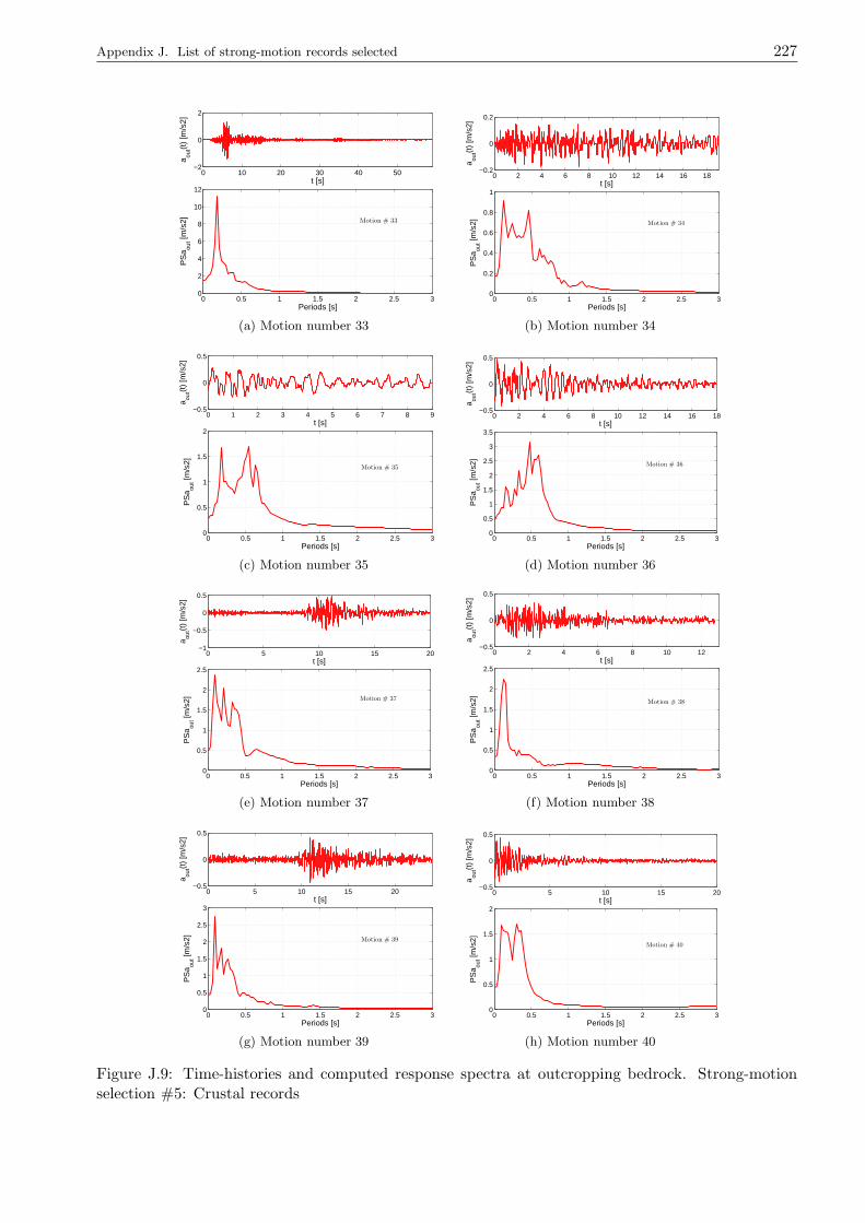
Appendix J. List of strong-motion records selected 227
0 10 20 30 40 50−2
0
2
t [s]a ou
t(t)
[m/s
2]
0 0.5 1 1.5 2 2.5 30
2
4
6
8
10
12
Motion # 33
Periods [s]
PS
a out [m
/s2]
(a) Motion number 33
0 2 4 6 8 10 12 14 16 18−0.2
0
0.2
t [s]
a out(t
) [m
/s2]
0 0.5 1 1.5 2 2.5 30
0.2
0.4
0.6
0.8
1
Motion # 34
Periods [s]
PS
a out [m
/s2]
(b) Motion number 34
0 1 2 3 4 5 6 7 8 9−0.5
0
0.5
t [s]
a out(t
) [m
/s2]
0 0.5 1 1.5 2 2.5 30
0.5
1
1.5
2
Motion # 35
Periods [s]
PS
a out [m
/s2]
(c) Motion number 35
0 2 4 6 8 10 12 14 16 18−0.5
0
0.5
t [s]
a out(t
) [m
/s2]
0 0.5 1 1.5 2 2.5 30
0.5
1
1.5
2
2.5
3
3.5
Motion # 36
Periods [s]
PS
a out [m
/s2]
(d) Motion number 36
0 5 10 15 20−1
−0.5
0
0.5
t [s]
a out(t
) [m
/s2]
0 0.5 1 1.5 2 2.5 30
0.5
1
1.5
2
2.5
Motion # 37
Periods [s]
PS
a out [m
/s2]
(e) Motion number 37
0 2 4 6 8 10 12−0.5
0
0.5
t [s]
a out(t
) [m
/s2]
0 0.5 1 1.5 2 2.5 30
0.5
1
1.5
2
2.5
Motion # 38
Periods [s]
PS
a out [m
/s2]
(f) Motion number 38
0 5 10 15 20−0.5
0
0.5
t [s]
a out(t
) [m
/s2]
0 0.5 1 1.5 2 2.5 30
0.5
1
1.5
2
2.5
3
Motion # 39
Periods [s]
PS
a out [m
/s2]
(g) Motion number 39
0 5 10 15 20−0.5
0
0.5
t [s]
a out(t
) [m
/s2]
0 0.5 1 1.5 2 2.5 30
0.5
1
1.5
2
Motion # 40
Periods [s]
PS
a out [m
/s2]
(h) Motion number 40
Figure J.9: Time-histories and computed response spectra at outcropping bedrock. Strong-motionselection #5: Crustal records

228 J.2. List of records compatible with French Antilles

Bibliography
Aki, K. and Richards, P. (2002). Quantitative Seismology: Theory and Methods. University ScienceBooks, Sausalito, California, USA, second edition edition.
Ambraseys, N., Douglas, J., Sigbjornsson, R., Berge-Thierry, C., P. Suhadolc, P., Costa, G., and Smit,P. (2004). Dissemination of european strong- motion data, vol. 2, using strong-motion datascapenavigator. Cd-rom collection, Engineering and Physical Sciences Research Council, United Kingdom.
Arias, A. (1970). A measure of earthquake intensity. In Seismic design for nuclear power plants, pages438–483. R.J. Hansen. MIT Press. Cambridge, Mass.
ATC 13 (1985). Erathquake damage evaluation data for california. Report atc, Applied TechnologyCouncil.
ATC 40 (1996). Seismic evaluation and retrofit of concrete buildings. Report atc, Applied TechnologyCouncil.
Aubert, P. (1997). Methodes MESHLESS en Geomecanique. These de doctorat, Ecole Centrale Paris.
Aubry, D., Chouvet, D., Modaressi, A., and Modaressi, H. (1985). GEFDYN 5, Logiciel d’analyse ducomportement statique et dynamique des sols par elements finis avec prise en compte du couplagesol-eau-air.
Aubry, D. and Clouteau., D. (1992). Recent Advances in Earthquake Engineering and StructuralDynamics, chapter A Subdomain Approach to Dynamic Soil-Structure Interaction, pages 251–272.Ouest Editions/AFPS, Nantes, France.
Aubry, D., Hujeux, J., Lassoudiere, F., and Meimon, Y. (1982). A double memory model with multiplemechanisms for cyclic soil behaviour. In Int. Symp. Num. Mod. Geomech., pages 3–13. Balkema.
Aubry, D. and Modaressi, A. (1992a). Strain localization in multipotential elastoplasticity. Interna-tional Journal for Numerical Methods in Engineering, 3(34):349–363.
Aubry, D. and Modaressi, A. (1996). GEFDYN,Manuel Scientifique.
Aubry, D., Modaressi, A., and Modaressi, H. (1990). A constitutive model for cyclic behaviour ofinterfaces with variable dilatancy. Computers and Geotechnics, 9(1):47–58.
Aubry, D. and Modaressi, H. (1989). Un modele de sols satures en dynamique non lineaire. RevueFrancaise de Geotechnique, (46):43–75.
Aubry, D. and Modaressi, H. (1992b). Seismic wave propagation in soils including non-linear andpore pressure effects. In: Recent Advances in Earthquake Engineering and Structural Dynamics, V.Davidovici (ed.), Ouest Editions, pages 209–224.
Aviles, J. and Perez-Rocha, L. (1996). Evaluation of interaction effects on the system period and thesystem damping due to foundation embedment and layer depth. Soil Dynamics and EarthquakeEngineering, 15:11–21.

230 Bibliography
Aviles, J. and Perez-Rocha, L. (2003). Soil-structure interaction in yieding systems. EarthquakeEngineering and Structrual Dynamics, 32:1749–1771.
Basu, U. and Chopra, A. (2003). Perfectly matched layers for time-harmonic elastodynamics of un-bounded domains: theory and finite-element implementation. Computer Methods in Applied Me-chanics and Engineering, 192(11-12):1337–1375.
Bathe, K. (1996). Finite Element Procedures. Pretince-Hall, New Jersey, USA.
Benzenatti, I. (1992). Modelisation du comportement dynamique des sols satures appliquee aux barrageset effets de site. These de doctorat, Ecole Centrale Paris.
Berenger, J. (1994). A perfectly matched layer for the absorption of electromagnetic waves. Journalof Computational Physics archive, 114(2):185–200.
Bielak, J., Loukakis, K., Hisada, Y., and Yoshimura, C. (2003). Domain reduction method for three-dimensional earthquake modeling in localized regions. part i: Theory. Bulletin of the SeismologicalSociety of America, 93(2):817–824.
Biot, M. (1962). Theory of propagation of elastic waves in a fluid-saturated porous solid. ii.- higherfrequency range. The Journal of Acoustical Society of America, 28(2):168–178.
Bommer, J. and Acevedo, A. (2004). The use of real earthquake accelerograms as input to dynamicanalysis. Journal of Earthquake Engineering, 8(1):43–91.
Chan, A. (1988). A unified Finite Element solution to Static and Dynamic Geomechanics. Ph.d.dissertation, University College of Swansea.
Chen, W. and Mizuno, E. (1990). Nonlinear analysis in soil mechanics. Elsevier, New York.
Choi, E., DesRoches, R., and Nielson, B. (2004). Seismic fragility of typical bridges in moderateseismic zones. Engineering Structures, 26(2):187–199.
Ciampoli, M. and Pinto, P. (1995). Effects of soil-structure interaction on inelastic seismic responseof brdige piers. Journal of Structural Engineering ASCE, 121(5):806–814.
Clayton, R. and Engquist, B. (1977). Absorving boundary conditions for acoustic and elastic waveequations. B.S.S.A., 67(6):1529–1540.
Clouteau, D. (1990). Propagation d’ondes dans des milieux heerogegenes, Application a la tenued’ouvrages sous seismes. These de doctorat, Ecole Centrale Paris.
Clouteau, D. (2000). ProMiss 0.2: Manuel Scientifique.
Clouteau, D. (2003). Miss 6.3: Manuel Utilisateur.
Clouteau, D. and Aubry, D. (2001). Computational Soil-Structure Interaction.
Clouteau, D. and Aubry, D. (2003). Boundary Element Methods for Soil-Structure Interaction, chapterComputational Soil-Structure Interaction, pages 61–126. Kluwer Academic Publishers.
de Martin, F. and Aochi, H. (2008). Radiation boundary condition using paraxial approximation.Report BRGM, BRGM.
Deodatis, G. (1996). Non-stationary stochastic vector processes: seismic ground motion applications.Probabilistic Enineering Mechanics, 11(149-168).
Dickenson, S. and Seed, R. (1996). Nonlinear dynamic response of soft and deep cohesive soil deposits.In Proc. of the International Workshop on Site Response Subjected to Strong Earthquake Motions.Yokosuka, Japan.
Bibliography 231
Douglas, J. (2006). Selection of strong-motion records for use as input to the structural models ofveda. Report BRGM BRGM/RP-54584-FR, BRGM.
Douglas, J., Roulle, A., Dominique, P., Maurin, C., and Dunand, F. (2005). Traitement des donneesaccelerometriques du conseil general de la martinique. rapport final. Report BRGM BRGM/RP-53906-FR, BRGM.
Engquist, B. and Majda, A. (1977). Absorbing boundary conditions for the numerical simulation ofwaves. Mathematics of Computation, 31(139):629–651.
EUROCODE 8 (2003). Design of structures for earthquake resistance, prEN 1998-1:200X. EuropeanStandard, European Committee for Standardization.
FEMA 356 (2000). Prestandard and commentary for the seismic rehabilitation of buildings. Reportfema, Federal Emergency Management Agency.
FEMA 450 (2003). NEHRP recommended provisions for seismic regulations for new buildings andother structures. provisions. commentary. Report fema, Federal Emergency Management Agency.
Fukushima, Y., Berge-Thierry, C., Volant, P., Griot-Pommera, D.-A., and Cotton, F. (2003). Atten-uation relation for west Eurasia determined with recent near-fault records from California, Japanand Turkey. Journal of Earthquake Engineering, 7(4):573–598.
Gasparini, D. and Vanmarcke, E. (1979). Simulated earthquake motions compatible with prescribedresponse spectra. Technical report, Departement of Civil Engineering, Massachusetts Institute ofTechnology, Cambridge, Massachusetts.
Gazetas, G. and Mylonakis, G. (2001). Soil-structure interaction effects on elastic and inelasticstructures. In Fourth International Conference on Recent Adavances in Geotechnical EarthquakeEngineering and Soil Dynamics. Symposium in Honor of Professor W.D. Liam Finn. San Diego,California.
Ghannad, M. and Jahankhah, H. (2007). Site-dependent strength reduction factors for soil-structuresystems. Soil Dynamics and Earthquake Engineering, 27:99–110.
Ghosh, B. and Madabhushi, S. P. G. (2003). Effects of localised soil inhomogenity in modyfyngseismic soil structure interaction. In 16th ASCE Engineering Mechanics Conference. University ofWashington, Seattle.
Giberson, M. (1969). Two nonlinear beams with definitions of ductility. Journal of Structural Division,ASCE, 95(2):137–157.
Hajal, T. (1984). Modelisation elasto-plastique des sols par une loi multimecanismes. Application aucalcul pressiometrique. These de doctorat, Ecole Centrale Pais, France, Chatenay-Malabry.
Hicher, P. and Rahma, A. (1994). Micro-macro correlations for granular media. Application to themodelling of sands. European Journal of Mechanics. A/Solids, 13(6):763–781.
Hughes, T. (1983). Computational Methods for Transient Analysis, chapter Analysis of TransientAlgorithms with Particular Reference to Stability Behavior, pages 67–155. North-Holland, Amster-dam.
Hughes, T. (2000). The Finite Element Method, Linear Static and Dynamic Finite Element Analysis.Dover Publications, Mineola, New York.
Hughes, T. and Liu, W. (1977a). Implicit explicit finite elements in transient analysis: Implementationand numerical examples. Journal of Applied Mechanics, (45):375–378.

232 Bibliography
Hughes, T. and Liu, W. (1977b). Implicit explicit finite elements in transient analysis: Stability theory.Journal of Applied Mechanics, (45):371–374.
Hughes, T., Pister, K., and Taylor, R. (1979). Implicit explicit finite elements in nonlinear transientanalysis. Computer Methods in Applied Mechanics and Engineering, (17/18):159–182.
Hujeux, J. (1979). Calcul numerique de problemes de consolidation elastoplastiques. These de doctorat,Ecole Centrale Paris, France.
Hujeux, J. (1985). Une loi de comportement pour le chargement cyclique des sols. In Genie Parasis-mique, pages 287–302. Presse ENPC.
Hwang, H. and Huo, J.-R. (1994). Generation of hazard-consistent fragility curves. Soil Dynamicsand Earthqauke Engineering, 13(5):34–354.
Ishihara, K. (1993). Liquefaction and flow failure during earthquakes. 33rd Rankine lecture. Geotech-nique, 43(3):351–415.
Iwasaki, T., Tatsuoka, F., and Takagi, Y. (1978). Shear moduli of sands under cyclic torsional shearloading. Soils and Foundations, 18(1):39–55.
Jennings, P. and Bielak, J. (1973). Dynamics of building-soil interaction. Bulletion of the SeismologicalSociety of America, 63:9–48.
Juang, C., Yuan, H., Li, D., Yang, S., and Christopher, R. (2005). Estimating severity of liquefaction-induced damage near foundation. Soils Dynamics and Earthquake Engineering, 25(5):403–11.
Kafali, C. and Grigoriu, M. (2007). Seismic fragility analysis: Application to simple linear and non-linear systems. Earthquake Engineering and Structural Dynamics, 36(13):1885–1900.
Kordjani, M. (1995). Caracterisation et modelisation du comportement en petites deformations dessols sur des chemins de sollicitation monotone et cyclique. These de doctorat, Ecole Centrale Paris,France.
Koutsourelakis, S., Prevost, J., and Deodatis, G. (2002). Risk assessment of an interacting structure-soil system due to liquefaction. Earthqauke Enginnering and Structural Dynamics, (31):851–879.
Kramer, S. (1996). Geotechnical Earthquake Engineering. Prentice Hall, New Jersey.
Lebrat, L., Morineau, A., and Piron, M. (2004). Statistique exploratoire multidimensionnelle. Dunod,Paris, 3eme edition edition.
Lemaitre, J. and Chaboche, J. (2001). Mecanique des materiaux solides. Dunod, Paris, 2eme editionedition.
Lopez-Caballero, F. (2003). Influence du comportement non lineaire du sol sur les mouvements sis-miques induits en geo-structures. These de doctorat, Ecole Centrale Paris.
Lopez-Caballero, F. and Modaressi, A. (2002). Identification des parametres pour la modelisation de laliquefaction des sables. In Symposium International- Identification et determination des parametresdes sols et des roches pour les calculs geotechniques, pages 189–198. Paris, Ed. J.P. Magnan, Pressesde l’Ecole Nationale des Ponts et Chaussees.
Lopez-Caballero, F., Modaressi, A., and Elmi, F. (2003). Identification of an elastoplastic modelparameters using laboratory and in-situ tests. In Deformation Characteristics of GeomaterialsISLyon 03, pages 1183–1190.
Bibliography 233
Lopez-Caballero, F., Modaressi, A., and Modaressi, H. (2007). Nonlinear numerical method for earth-quake site response analysis i- elastoplastic cyclic model & parameter identification strategy. Bulletinof Earthquake Engineering, 5(3).
Lopez-Caballero, F. and Modaressi-Farahmand Razavi, A. (2008). Numerical simulation of liquefactioneffects on seismic ssi. Soil Dynamics and Earthquake Engineering, 28(2):85–98.
Luco, J. (1980). Soil-structure interaction and identification of structural models. In Proceedings ofthe ASCE Specially Conference in Civil Engineering and Nuclear Power. Tennessee.
Luong, M. (1980). Phenomenes cycliques dans les sols pulverulents. Revue Francaise de Geotechnique,10(1):39–53.
Maison, F. (1992). PC-ANSR: A Computer program for Nonlinear Structural Analysis.
Marante, M., Suarez, L., Quero, L., j. Redondo, Vera, J., Uzcategui, M., Delgado, S., Leon, L., nez,L. N., and Florez, J. (2005). Portal of damage: a web-based finite element program for the analysisof framed structrues subjected to overloads. Advances in Engineering Software, 36:346–358.
Marin, S., Avouac, J., Nicolas, M., and Schlupp, A. (2004). A probabilistic approach to seismic hazardin metropolitan france. Bulletin of the Seismological Society of America, 94(6):2137–2163.
Martin, C., Combes, P., Secanell, R., Lignon, G., Fioravanti, A., Carbon, D., Monge, O., and Grellet,B. (2002). Revision du zonage sismique de la france : Etude probabiliste. Rapport de Phase 3Affaire no. 1601, Report GTR/MATE/0701-150.
Mellal, A. (1997). Analyse des effets du comportement non lineaire des sols sur le mouvement sismique.These de doctorat, Ecole Centrale Paris, France.
Michali, A. (1994). Methode pour l’identification des parametres d’une loi elastoplastique a partird’essais de laboratoire et in-situ. These de doctorat, Ecole Centrale Paris, France.
Michalski, E. and Rahma, A. (1989). Modelisation du comportement des sols en elastoplasticite :definition des parametres des modeles Hujeux- Cyclade et recherche des valeurs des parametrespour differents sols. 89 SGN 117 GEG, Bureau de Recherches Geologiques et Minieres BRGM.
Miranda, E. and Vertero, V. (1994). Evaluation of strength reduction factors for earthquake-resistantdesign. Earthquake Spectra, 10(2):357–379.
Modaressi, A. (2003). Modelisation des milieux poreux sous chargements complexes. Diplomed’habilitation a diriger des recherches, Institut National Polytechnique de Grenoble, Grenoble.
Modaressi, A. and Lopez-Caballero, F. (2001). Global methodology for soil behavior identificationand its application to the study of site effects. In 4th International Conference on recent Advancesin Geotechnical Earthquake Engineering and Soil Dynamics, page 1.08. San Diego, California. Eds.Prakash.
Modaressi, H. (1987). Modelisation numerique de la propagation des ondes dans les milieux poreuxanelastiques. These de doctorat, Ecole Centrale Paris.
Modaressi, H. and Aubry, D. (1989). On the dynamic behaviour of an elastoplastic constitutive modelfor soils. In Soil Dynamics and Liquefaction, Proceedings of the Fourth International Conferenceon Soil Dynamics and Earthquake Engineering, Mexico City, Mexico, pages 53–60. ComputationalMechanics Publications, Southampton, England and Boston.
Modaressi, H., Aubry, D., Faccioli, E., and Noret, C. (1995). Numerical modelling approaches for theanalysis of the earthquake triggered landslides. In 3rd International Conference on recent Advancesin Geotechnical Earthquake Engineering and Soil Dynamics, volume II, pages 833–843. St. Louis,Missouri. Eds. Prakash.
234 Bibliography
Modaressi, H. and Benzenati, I. (1994). Paraxial approximation for poroelastic media. Soil dynamicsand Earthquake Engineering, 13(2):117–129.
Modaressi, H. and Foerster, E. (2000). CyberQuake. User’s manual, BRGM, France.
Nau, R., Oliver, R., and Pister, K. (1982). Simulating and analyzing artificial nonstationary earthquakeground motions. Bulletin of the Seismological Society of America, 72:615–636.
NIST/SEMATECH (2006). Nist/sematech e-handbook of statistical methods.http://www.itl.nist.gov/div898/handbook/.
Park, Y. and Ang, A. (1985). Mechanistic seismic damage model for reinforced concrete. Journal ofStructural Engineering, ASCE, 111(4):722–739.
Pecker, A. (1984). Dynamique des sols. Presses de ECOLE Nationale des Ponts et Chaussees, Champssur Marne.
Pianka, C. (1998). Contribution to soil/structure and user interfaces in geomechanics. These dedoctorat, Ecole Centrale Paris.
Piccuezzu, E. (1991). Lois de Comportement en Geomecanique; Modelisation, Mise en oeuvre, Iden-tification. These de doctorat, Ecole Centrale Paris.
Pitilakis, D. (2006). Soil-Structure Interaction Modeling Using Equivalent Linear Soil Behavior InThe Substructure Method. These de doctorat, Ecole Centrale Paris.
Popescu, R. (2002). Finite element assessment of the effects of seismic loading rate on soil liquefaction.Canadian Geotechnical Journal, 39(2):331–344.
Popescu, R., Prevost, J., and Deodatis, G. (2005). 3d effects in seismic liquefaction of stochasticallyvariable soil deposits. Geotechnique, 55(1):21–31.
Popescu, R., Prevost, J., Deodatis, G., and Chakrabortty, P. (2006). Dynamics of nonlinear porousmedia with applications to soil liquefaction. Soil Dynamics and Earthquake Engineering, 26(2):648–665.
Poulos, H. and Davis, E. (1974). Elastic Solutions for Soil and Rocks Mechanis. Wiley, New York.
Pousse, G., Bonilla, L., Cotton, F., and Margerin, L. (2006). Nonstationary stochastic simulation ofstrong ground motion time histories including natural variability: application to the K-Net Japanesedatabase. Bulletin of the Seismological Society of America, 96(6):2103–2117.
Prakash, V., Powel, G., and Campbell, S. (1993). DRAIN 2D-X, Base program description and UserGuide.
Priestley, M. and Parck, R. (1987). Strength and ductility of concrete bridges columns under seismicloading. ACI Structural JOURNAL, 84(1):61–76.
PS-92 (1999). Regles PS applicables aux batiments - PS-92. Regles de construction parasismique.,Norme Francaise NF P 06-013.
Rahma, A. (1988). Modelisation probabiliste des parametres de lois elasto-plastiques - Modele Cyclade.These de doctorat, Ecole Centrale Paris.
Rathje, E., Abrahamson, N., and Bray, J. (1998). Simplified frequency content estimates of earthquakeground motions. Journal of Geotechnical and Geoenvironmental Engineering, 124(2):150–159.
Rodriguez, M. and Montes, R. (2000). Seismic response and damage analysis of building supportedon flexible soils. Earthquake Engineering and Structural Dynamics, 29:647–665.
Bibliography 235
Sabetta, F. and Pugliese, A. (1996). Estimation of response spectra and similation of nonstationaryearthquake ground motions. Bulletin of Seismological Society of America, 86(2):337–352.
Saez, E. (2005). Prise en compte de la non-linearite du comportement du sol sur les effets del’interaction sol structure en dynamique. Memoire de master, Ecole Nationle des Ponts et Chaussees.
Saez, E. (2007). Poutre 33 v1.1. Gefdyn technical note, Ecole Centrale Paris.
Saez, E., Lopez-Caballero, F., and Modaressi, A. (2006). Effects of ssi on the capacity spectrummethod. In Proc. First European Conference on Earthquake Engineering and Seismology, page id1073.
Saez, E., Pitilakis, D., Lopez-Caballero, F., and Modaressi, A. (2007). Evaluation of non linear ssieffects following an equivalent linear approach. In Proc. 5th International Conference on Seismologyand Earthquake Engineering, page SF65. Tehran, Iran.
Saporta, G. (2006). Probabilites, analyse des donnees et statistique. TECHNIP, Paris, 2eme editionedition.
Saragoni, G. and Hart, G. (1974). Simulation of artificial earthquakes. Earthquake Engineering andSoil Dynamics, 2:249–267.
Schnabel, P., Lysmer, J., and Seed, H. (1972). Shake: a computer program for earthquake responseanalysis of horizontally layered sites. Report EERC-72-12, Earthquake Engineering ResearchCenter, University of California, Berkeley, CA.
Schofield, A. and Wroth, C. P. (1968). Critical State Soil Mechanics. McGraw-Hill, London.
Seed, H. B. and Idriss, I. M. (1982). Ground motion and soil liquefaction during earthquakes. Mono-graph series, earthquake engineering research institute, University of California, Berkeley, CA.
Seed, H. B., Wong, R. T., Idriss, I. M., and Tokimatsu, K. (1986). Moduli and damping factors fordynamic analyses of cohesionless soils. Journal of Geotechnical Engineering - ASCE, 112(11):1016–1032.
Seekins, L., Brady, A., Carpenter, C., and Brown, N. (1992). Digitized strong-motion accelerogramsof north and central american earthquakes 1933-1986. Cd-rom, Digital Data Series DDS-7.
Shinozuka, M. (1998). Statical analysis of bridge fragility curves. In Proceedings of the US-ItalyWorkshop on Protective Systems for Bridges. New York, N.Y.
Shinozuka, M., Feng, Q., Lee, J., and Naganuma, T. (2000). Statistical analysis of fragility curves.Journal of Engineering Mechanics, 126(12):1224–1231.
Sica, S. (2001). Analisi del comportamento dinamico di dighe in terra. Dottorati di ricerca, Universitadegli Studi di Napoli Federico II, Italia.
Tokimatsu, K., Mizuno, K., and Kakurai, H. (1996). Building damage associated with geotechnicalproblems. Soils Found - Special Issue, (1):219–32.
Trifunac, M. and Brady, A. (1975). A study on the duration of strong earthquake ground motion.Bulletin of the Seismological Society of America, 65(3):581–626.
HAZUS-MH MR3 (2003). Multi-hazard Loss Estimation Methodology. Technical Manual. ReportFEMA, Federal Emergency Management Agency.
van der Vaart, A. (2000). Asymptotic Statistics (Cambridge Series in Statistical and ProbabilisticMathematics). Cambridge University Press.

236 Bibliography
Vecchio, F. and Emara, M. (1992). Shear deformation in reinforced concrete frames. ACI StructuralJournal, 89(6):45–56.
Veletsos, A. (1977). Structural and Geotechnical Mechanics, chapter Dynamic of structure-foundationsystems, pages 333–361. Prentice-Hall, Englewood Cliffs, NJ.
Veletsos, A. and Meek, J. (1974). Dynamic behavior of building-foundation systems. EarthquakeEngineering and Structural Mechanics, 3:121–138.
Veletsos, A. and Nair, V. (1975). Seismic interaction of structures on hysteretic foundations. Journalof the Structural DIVISION (ASCE), 101:109–129.
Wolf, J. (1985). Dynamic Soil-Structure Interaction. Prentice Hall, Englewood Cliffs, New Jersey.
Wolf, J. and Song, C. (1996). Finite-element modelling of unbounded media. John Wiley & Sons,Baffins Lane, England.
Yamashita, S., Kohata, Y., Kawaguchi, T., and Shibuya, S. (2001). International round-robin testorganized by TC-29. In Advanced Laboratory Stress-Strain Testing of Geomaterials, pages 60–82.Tatsuoka, Shibuya & Kuwano (eds), Balkema Publishers.
Zienkiewicz, O., Bicanic, N., and Shen, F. (1988). Earthquake input definition and the transmittingboundary conditions. In Doltsinis, I. S., editor, Advances in Computational Nonlinear Mechanics,pages 109–138. Springer-Verlag.
Zienkiewicz, O., Chan, A., Pastor, M., Schrefler, B., and Shiomi, T. (1999). Computational Ge-omechanics with Special Reference to Earthquake Engineering. Wiley, Baffins Lane, Chichester,England.
Zienkiewicz, O., Chang, C., and Bettless, P. (1980). Drained, undrained, consolidating and dynamicbehaviour assumption in soils; limits of validity. Geotechnique, (30):385–395.
Zienkiewicz, O. and Shiomi, T. (1984). Dynamic behaviour of saturated porous media: The generalizedbiot formulation and its numerical solution. International Journal of Numerical and AnalyticalMethods of Geomechanics, (8):71–96.