Draft - 2

Missouri River Recovery Management Plan – Climate Change Assessment

HYDROLOGIC ENGINEERING BRANCH

ENGINEERING DIVISION December 2016

Climate Change Assessment – Missouri River Basin

DRAFT

Draft - 3

TABLE OF CONTENTS 1 Introduction ........................................................................................................................................... 5

2 Project Description ................................................................................................................................ 5

3 Project Purpose ..................................................................................................................................... 6

4 Relevant Current Climate and Climate Change literature review ......................................................... 7

4.1 USACE Climate Change Adaptation Pilots .................................................................................. 7

4.1.1 Climate Change Sediment Yield Impacts on Operations Evaluations at Garrison Dam, North Dakota (USACE-NWO, September 2012) ........................................................................................... 7

4.1.2 Climate Change Impacts on the Operation of Coralville Lake, Iowa (USACE-CEMVR, September 2012) ................................................................................................................................... 8

4.1.3 Upper Missouri River Basin Mountain Snowpack – Accumulation and Runoff (USACE-MRBWM, July 2014) ........................................................................................................................... 8

4.2 Changes Towards Earlier Streamflow Timing Across Western North America (Stewart et al, 2005) 9

4.3 West-Wide Climate Risk Assessments (USBR, March 2011) ........................................................ 9

4.4 Regional Climate Trends and Scenarios for the US National Climate Assessment (NOAA, 2013) 10

4.5 Literature Synthesis on Climate Change Implications for Water and Environmental Resources (USBR, Jan. 2011) .................................................................................................................................. 10

4.6 Recent US Climate Change and Hydrology Literature Applicable to US Army Corps of Engineers Missions (USACE Institute for Water Resources, Jan. 2015) ................................................................ 11

4.7 Hydrological Variability and Uncertainty of Lower Missouri River Basin Under Changing Climate (Qiao et al, 2013) ....................................................................................................................... 12

4.8 Summary ..................................................................................................................................... 12

5 Changes to Regional Hydrology and Assessment of Vulnerability using climate change tools......... 13

5.1 National Climate Change Viewer (USGS, 2013) ....................................................................... 14

5.2 Nonstationarity Detection Tool and Climate Hydrology Assessment Tool (USACE, 2016) ...... 14

5.2.1 Missouri River at Rulo ........................................................................................................ 16

5.2.2 Missouri River at Hermann ................................................................................................. 19

5.2.3 Yellowstone River at Billings ............................................................................................. 22

5.2.4 James River at LaMoure ..................................................................................................... 25

5.2.5 Niobrara River at Sparks ..................................................................................................... 28

5.2.6 Platte River at Louisville ..................................................................................................... 31

5.2.7 Nishnabotna River above Hamburg .................................................................................... 34

5.2.8 Kansas River at Topeka ...................................................................................................... 36

5.2.9 Summary of Results ............................................................................................................ 39

5.3 Watershed Vulnerability Assessment Tool (USACE, 2016) ....................................................... 40

5.3.1 Flood Risk Reduction.......................................................................................................... 40

5.3.2 Ecosystem Restoration ........................................................................................................ 43

Draft - 4

5.3.3 Summary of Results ............................................................................................................ 47

6 Climate Change Effects on Study Alternatives ................................................................................... 47

6.1 Alternatives Summary................................................................................................................. 47

6.1.1 Alt1a_NoAction .................................................................................................................. 47

6.1.2 Alt2a_BiOp ......................................................................................................................... 48

6.1.3 Alt3a_Mech ......................................................................................................................... 49

6.1.4 Alt4a_Spring2-42MAF ....................................................................................................... 50

6.1.5 Alt5a_Fall5-35SL................................................................................................................ 50

6.1.6 Alt6a_SpawningCue ........................................................................................................... 51

6.2 Climate Change Conclusions ...................................................................................................... 54

7 REFERENCES ................................................................................................................................... 57

8 Attachment: USGS Climate Change Viewer Results ........................................................................ 59

Draft - 5

1 INTRODUCTION A qualitative climate change assessment for the Missouri River Recovery Management Plan was performed by the United States Army Corps of Engineers (USACE) in accordance with Engineering and Construction Bulletin: Guidance for Climate Change Adaptation Engineering Inputs to Inland Hydrology for Civil Works Studies, Designs, and Projects (ECB 2016-25, USACE, September 2016). A cursory look at primary references regarding climate change within the Missouri River basin was performed previously, and it was recommended that more extensive reviews be carried out as part of the full qualitative analysis in this phase of the study. The climate change assessment results were also examined to determine their effects on various plan alternatives being considered at this phase of the study.

2 PROJECT DESCRIPTION The Missouri River Recovery Management Plan is part of the Missouri River Recovery Program (MRRP), which is the umbrella program that works to coordinate activities on the Missouri River for restoration of native habitats and to comply with the Endangered Species Act and 2003 Biological Opinion. The Missouri River Recovery Management Plan involves the creation of a detailed suite of models for the Missouri River basin that aid in the evaluation of scenarios reflecting a wide-range of hydrologic conditions. Missouri River H&H modeling consists of the latest versions of five Hydrologic Engineering Center (HEC) modeling components or software programs that were used in concert with one another to meet the input/output needs of the MRRP:

• Hydrologic Engineering Center-River Analysis System (HEC-RAS): Designed to perform one-dimensional hydraulic calculations for a full network of natural and constructed channels. Allows users to perform steady flow water surface profile computations, unsteady flow simulation, sediment transport computations, and water temperature modeling. The MRRP will focus on steady and unsteady flow modeling to identify a base condition, which will be compared and assessed with future management alternatives. Common H&H outputs include stage, duration/timing of inundation, water velocities, flow areas/routes, water temperature, and sediment loads.

• Hydrologic Engineering Center-Reservoir System Simulation (HEC-ResSim): Software for use in

modeling reservoir operations at one or more reservoirs with varying operational goals and constraints. Allows users to simulate period-of-record reservoir operations for a variety of alternatives.

• Hydrologic Engineering Center-Ecosystem Functions Model (HEC-EFM): Created to help study

teams determine ecosystem responses to changes in the flow regime of a river or connected wetlands. Typical HEC-EFM analysis include: 1) statistical analyses of relationships between hydrology and ecology, 2) hydraulic modeling, and 3) the use of Geographic Information Systems (GIS) to display results and spatial data. The MRRP will use these modeling results to help define existing ecological conditions, highlight potential restoration areas, and assess/rank alternative conditions according to predicted changes in the system.

• Hydrologic Engineering Center-Flood Impact Analysis (HEC-FIA): Designed to calculate post-

flood or forecasted-flood damages and to determine the flood damage reduction benefits attributed

Draft - 6

to flood control projects (reservoirs and levees). HEC-FIA modeling outputs for observed or forecasted hydrographs include: 1) flood damage estimates for urban and agricultural structures/property, population at risk, and life loss, 2) real-time flood operation decision-support activities, 3) post-flood impact assessments for disaster relief, and 4) post-flood and annual assessments of Corps project benefit accomplishments. The MRRP will use HEC-FIA modeling results to identify baseline and future with project impacts on social, cultural, and economic resources within the basin.

• (Potential Future Model) Hydrologic Engineering Center-Watershed Analysis Tool (HEC-WAT):

Provides a common graphical user interface to integrate and incorporate software packages (i.e., HEC-RAS, HEC-ResSim, HEC-EFM, etc), while the individual pieces of software provide the analytical computations. Allows the user to perform hydrologic, hydraulic, environmental, and planning analyses from a single interface. HEC-WAT is designed to facilitate: 1) data entry into individual modeling programs from a single location, 2) identification and definition of study alternatives, 3) trade-off analyses of multiple alternatives, 4) enhanced study team coordination through shared displays and reports, and 5) review of modeling results from a single, direct location.

The Missouri River models were created as base models for planning studies which are used to simulate and analyze broad-scale watershed alternatives. The objective of this assessment is to analyze climate change and its possible qualitative effects on the alternatives currently being considered.

3 PROJECT PURPOSE As part of the Missouri River Recovery Management Plan, various alternatives were developed that could potentially assist in the recovery of the threatened and endangered species along the Missouri River. Impacts of those alternatives on the other seven authorized purposes were assessed. Any future conditions that change the hydrology of the basin could change the magnitude of those impacts. Therefore, it is important to understand how climate may impact the basin. Various alternatives being considered in this study propose adding additional release requirements to the System regulation at different times of year in the hopes of creating sandbar habitat from the changes in releases. One alternative uses mechanical methods, rather than System releases, to create sandbar habitat. Climate change was considered with regards to these various alternatives and their hydrologic effects (flow, temperature, snowmelt, and sedimentation) to aid in the selection of a final alternative. Extending the climate change assessment to specific species or habitat impacts is beyond the scope of this study. USACE projects, programs, missions, and operations have generally proven to be robust to the range of natural climate variability over their operating life spans. Recent scientific evidence shows, however, that in some places and for some impacts relevant to USACE operations, climate change is shifting the climatological baseline about which that natural climate variability occurs, and may be changing the range of that variability as well. This is important to USACE because the assumptions of stationary climatic baselines and a fixed range of natural variability as captured in the historical hydrologic record may no longer be appropriate for long-term projections of the climatologic parameters, which are important in hydrologic assessments for inland watersheds. This document was prepared in accordance with the USACE overarching climate change adaptation policy that requires consideration of climate change in all current and future studies to reduce vulnerabilities and enhance the resilience of our water-resource infrastructure.

Draft - 7

4 RELEVANT CURRENT CLIMATE AND CLIMATE CHANGE LITERATURE REVIEW

The current climate in the Basin consists of large temperature fluctuations and extremes, due to its mid-continent location. Winters are generally cloudy and cold over the majority of the area, while summers range from fair to very hot and humid. Temperature extremes range from winter lows of -60 degrees Fahrenheit (°F) in Montana to summer highs of 120 °F in the lower basin (U.S. Army Corps of Engineers 2006). The Basin experiences tremendous variability in runoff, ranging from numerous periods of extreme droughts to numerous periods of extreme floods. Most recently, the Basin was dramatically impacted by the sudden 2012 drought immediately following the 2011 record runoff year. Numerous publications on climate change from varying sources were reviewed and summarized during the literature review portion of Phase 1. The consensus was that temperature and precipitation in the Missouri River basin have increased. The increased temperatures cause less winter precipitation to fall as snow and more to fall as rain resulting in less mountain snowpack accumulation throughout the western portion of the basin. With more winter precipitation falling as rain, runoff increases during the winter months. The snowpack that does accumulate during the winter months is melting earlier resulting in earlier peaks in the seasonal mountain runoff patterns. The northern plains are experiencing similar changes with more rainfall and less snowpack accumulating during winter months resulting in earlier peaks in seasonal plains runoff patterns. Annual rainfall amounts have increased during the summer months, but rainfall events have become sporadic for the entire Missouri River basin. Large rain events are more frequent and interspersed by longer relatively dry periods. Sediment loading and inflows are expected to increase into Garrison Reservoir in the upper basin for all climate scenarios evaluated. More details from each specific source are given below.

4.1 USACE CLIMATE CHANGE ADAPTATION PILOTS USACE is improving knowledge about climate change impacts and adaptation by conducting targeted pilot studies to test new ideas and to develop and utilize information at the project-level scale, and to glean information needed to develop policy and guidance. Through these pilots, USACE is developing and testing alternative adaptation strategies to achieve specific business management decisions; identify new policies, methods, and tools to support adaptation for similar cases; learn how to incorporate new and changing climate information throughout the project lifecycle; develop, test, and improve an agency level adaptation implementation framework; and to implement lessons learned. As of 2012, USACE had 15 or more targeted pilot studies scoped for completion by various Divisions and Districts within USACE. Three of those studies applicable to the Missouri River basin had been completed by the time of this climate change analysis, and are summarized in the following sections. The complete list of pilot studies can be seen in Climate Change Adaption Pilots (USACE, September 2012).

4.1.1 Climate Change Sediment Yield Impacts on Operations Evaluations at Garrison Dam, North Dakota (USACE-NWO, September 2012)

This study used statistically downscaled regional climate projections for five different climate scenarios: drier and cooler, drier and warmer, wetter and cooler, wetter and warmer, and a median future precipitation and temperature condition. Measured stream gage data and historic reservoir survey data were used to develop sediment rating curves to define the streamflow-sediment relationship. The Variable Infiltration Capacity (VIC) model flows were applied to this relationship to estimate the change in reservoir capacity. The six mainstem Missouri River dams were simulated as a system using the Daily Routing Model (DRM); as the pool elevations and releases increase at Garrison Dam, the operations of the other five reservoirs can be adjusted to compensate. This helped reduce the overall effect of the increased flows into the system. Key findings were:

Draft - 8

• All climate change scenarios evaluated resulted in an increase in sediment loading and inflows. • Climate-adjusted flows can have a large impact on pool elevations and releases for all climate

scenarios evaluated. • Impacts from changing sedimentation rates on flood regulation would be minor for this large

mainstem reservoir, but hydrologic changes could potentially be significant.

4.1.2 Climate Change Impacts on the Operation of Coralville Lake, Iowa (USACE-CEMVR, September 2012)

This study used a risk-based approach to identify the most likely, highest consequence impacts that may result from climate change. The study identified key performance questions and metrics, such as 15‐day peak inflow and time until allocated sediment storage is fully utilized, for the highest risk of potential impacts from climate change on project performance. Based on quantitative analysis using downscaled climate projections, potential adaptation strategies were developed and are being tested for effectiveness across a range of possible future climate scenarios. Some applicable findings from this study are: • Upward trends in average annual temperature and total annual precipitation have been observed

in Iowa between the early 20th and early 21st century, and at the tested gauges within the Iowa River Basin. These trends are statistically significant at 95 percent confidence.

• There also has been an observed increase in the occurrence of the heaviest precipitation events (i.e., more days of heavy precipitation per year).

• All climate scenarios except one indicate that sedimentation rates are likely to increase over historical rates, consistent with increases in precipitation and streamflow.

4.1.3 Upper Missouri River Basin Mountain Snowpack – Accumulation and Runoff (USACE-MRBWM, July 2014)

This study analyzed precipitation, air temperature, relative humidity, soil moisture, potential evapotranspiration, and climate patterns for the two reaches of Garrison upstream to Fort Peck, and Fort Peck to the upstream limits of the Missouri River Basin. These parameters were analyzed for statistically significant trends and correlation factors, then used to develop multiple linear regression equations. The period of record used for analysis varied from 50 to 116 years, depending on the availability of data for the specific parameter being analyzed. The outputs of the Community Climate Systems Model (CCSM3 & CCSM4) Atmosphere-Ocean General Circulation Models (AOGCM) for 2012-2099 were fed into multiple linear regression equations developed based on historical data to determine the projected trends. The results most applicable to this climate change assessment are summarized below. • Average basin temperatures had statistically significant upward historic trends. Average basin

precipitation, evapotranspiration, and soil moisture did not have statistically significant historic trends.

• The date snowpack begins accumulating had a statistically significant later historic trend for the Garrison reach, but no statistically significant historic trend for the Fort Peck reach. There was no statistically significant trend in peak snow water equivalent (SWE).

• Annual and May-June-July runoff at Garrison had a statistically significant downward trend over the period of record. No statistically significant trend was detected for Fort Peck.

• Of the 4 stream gages analyzed, only one had a statistically significant downward historic trend in annual streamflow. None had statistically significant historic trends in May-June-July streamflow.

The table below, copied from Upper Missouri River Basin Mountain Snowpack – Accumulation and Runoff (2014), summarizes the study’s findings for both historical trends and projected trends from climate models out to year 2100.

Draft - 9

DSBA – Date Snowpack Begins Accumulating. MJJ – May, June, July. SWE – Snow Water Equivalent. ENSO – El Nino Southern

Oscillation. NAO – North Atlantic Oscillation. DPS – Date of Peak SWE. DMO – Date of Melt-out. Table 4-1. Summary Findings from Upper Missouri River Basin Mountain Snowpack –

Accumulation and Runoff.

4.2 CHANGES TOWARDS EARLIER STREAMFLOW TIMING ACROSS WESTERN NORTH AMERICA (STEWART ET AL, 2005)

This report is a statistical analysis covering changes in the timing of snowmelt and streamflow across western mountainous states across North America from 1948 to 2002. • Results show trends in both earlier onset of the snowmelt pulse and earlier CT timing (center of

mass of the annual flow), and although the overall average streamflow at most locations remained similar, the timing was from ten to 30 days earlier in the start of the snowmelt season during the period of analysis.

4.3 WEST-WIDE CLIMATE RISK ASSESSMENTS (USBR, MARCH 2011) This report is a thorough overview of a climate change forecast modeled in 2011. The report shows a hydroclimatic projection of the Missouri Basin above Omaha. The model used initial flow data from

Draft - 10

the NRCS and NWS, and projected the model results forward up to 80 years starting with a 30 year increment from 1990 to 2020, moving to a midpoint of 1990 to 2050, and completing with results covering 1990 to 2070. The projected models used monthly data. The modeled climate results showed an overall increasing trend in rainfall throughout the region, despite a decrease in April 1st SWE values. Overall mean annual runoff values showed an increasing trend as did overall average temperatures in the basin. The Reclamation report compared model results with a defined 50th percentile mean to illustrate median climate change conditions forecast out into 2070. The strongest signal was the change forecast in Annual Mean Temperature though 2070 in which the basin average temperature increases from around 43 degrees F in 1990 to near 50 degrees F by 2070. Total precipitation also shows an increase, from an annual basin average of about 18 inches in 1990 to near 20 inches by 2070. While precipitation did not exhibit as great a variation as temperatures, the timing of rainfall and snowmelt did change, with rain events occurring later in the year, and snowmelt occurring earlier in the spring, which made overall snow water equivalent (SWEs) trends decrease by 2070. The limitations of the model used by Reclamation in this report were addressed to a great extent. Some of the more significant model limitations include; model results limited to model parameters that do not account for all of the uncertainties in climate modeling (aerosols, smaller terrain features, mesoscale circulations etc.), limits of the spatial resolution of a downscaled model on runoff and location specific effects of the limited calibration of the model. A major caveat to all snow-related findings of this study are the residual biases associated with generating conclusions that require projected climate data at less than a monthly time scale. Data at less than a monthly time interval are necessary to adequately analyze changes in snowmelt season duration and melt date.

4.4 REGIONAL CLIMATE TRENDS AND SCENARIOS FOR THE US NATIONAL CLIMATE ASSESSMENT (NOAA, 2013) The report details effects from different modeled emissions scenarios including a higher emission scenario and a lower emission scenario. Effects from these two modeled scenarios focus on the sociological effects of changes in temperature and precipitation, and although the report addresses climate change, it does not give details on effects for specific hydrologic/meteorologic events. Conclusions include: • Rising temperatures in the Great Plains will increase the demand for water, which could stress

natural resources and increase competition for water among communities. • Changes in temperatures could influence crop growth cycles due to warming winters and

changes in rainfall patterns which may require new agriculture and livestock management practices.

• The magnitude of expected changes in climate could exceed the extremes experienced in the last century, rendering existing adaptation and planning efforts as inadequate for responding to the future impacts from climate change. Extremes in climate will also magnify periods of wet or dry weather resulting in longer, more severe droughts, and larger more extensive flooding.

4.5 LITERATURE SYNTHESIS ON CLIMATE CHANGE IMPLICATIONS FOR WATER AND ENVIRONMENTAL RESOURCES (USBR, JAN. 2011) The scope of this report was to offer a summary of recent literature on the past and projected effects of climate change on hydrology and water resources and then to summarize implications for key resource areas featured in Reclamation planning processes. In preparing the synthesis, the literature review considered documents pertaining to general climate change science; climate change as it relates to

Draft - 11

hydrology, water resources, and environmental resources; and application of climate change science. Sample results include: • Over the course of the 20th century, it appears that all areas of the Great Plains (GP) Region

became warmer, and some areas received more winter precipitation during the 20th century. Cayan et al. (2001) report that Western United States spring temperatures have increased 1–3 °C (1.8–5.4 °F) since the 1970s. Based on data from the USHCN, temperatures have risen approximately 1.85 °F (1.02 °C) in the northern Great Plains between 1901 and 2008. That dataset also reveals an increase in annual precipitation of more than 4% in the northern Great Plains.

• Coincident with these trends, the western GP Region also experienced a general decline in spring snowpack, reduced snowfall to winter precipitation ratios, and earlier snowmelt runoff.

• Future climate conditions will feature less snowfall and more rainfall, less snowpack development, and earlier snowmelt runoff. Warming will lead to more intense and heavy rainfall that will tend to be interspersed with longer relatively dry periods.

• Gutowski et al. (2008) suggested that climate change likely will cause precipitation to be less frequent but more intense in many areas and suggests that precipitation extremes are very likely to increase.

• Snow accumulation, while important on the western headwaters of the Missouri system, plays only a modest role in total system runoff; and reduced precipitation combined with increasing potential evapotranspiration play a major role in system runoff reductions (Lettenmaier et al. 1999).

• Chapter 5 of SAP 4.3 discusses how biodiversity may be affected by climate change (Janetos et al. 2008) and indicates that many studies have been published on the impacts of climate change for individual species and ecosystems. Predicted impacts are primarily associated with projected increases in air and water temperatures and include species range shifts poleward, adjustment of migratory species arrival and departure, amphibian population declines, and effects on pests and pathogens in ecosystems.

4.6 RECENT US CLIMATE CHANGE AND HYDROLOGY LITERATURE APPLICABLE TO US ARMY CORPS OF ENGINEERS MISSIONS (USACE INSTITUTE FOR WATER RESOURCES, JAN. 2015)

This report is 1 of 21 regional climate syntheses prepared at the scale of 2-digit USGS Hydrologic Unit Codes (HUC) across the US. These reports summarize observed and projected climate trends. Some findings of importance for the Missouri River region are summarized below. Conclusions are consistent with findings from other sources for the area. • An observed trend in earlier spring onset and earlier spring warming was found by 3 different

studies. • An increasing trend in observed mean and daily minimum air temperature was observed;

however, a trend in daily maximum air temperature is lacking. • A mild upward trend in annual and extreme precipitation in the lower portion of the Missouri

River Basin has been identified by multiple authors, while the upper portion has been identified to have a decreasing trend for annual and extreme precipitation.

• A mild upward trend in mean streamflow for the Missouri River Region has been identified by multiple authors, but a clear consensus is lacking in the upper portion of the region.

• USACE vulnerability assessments indicate a strong consensus that air temperatures will trend upward over the next century.

• There is less consensus on projected trends for precipitation, but most studies report a general increase in precipitation for the region.

Draft - 12

• Consensus is lacking regarding the direction of projected trends in streamflow, runoff, and water yield.

4.7 HYDROLOGICAL VARIABILITY AND UNCERTAINTY OF LOWER MISSOURI RIVER BASIN UNDER CHANGING CLIMATE (QIAO ET AL, 2013)

The North American Regional Climate Change Assessment Program (NARCCAP) climate projections were used as atmospheric forcing for the Soil and Water Assessment Tool (SWAT) model which runs with varying potential evapotranspiration (PET) methods to assess the hydrological change and uncertainty of 2040-2069 over 1968-1997. The NARCCAP temperature and precipitation predictions were refined using a bias correction method. Key findings from the study were:

• Expected precipitation tends to increase in intensity with little change in frequency, triggering faster surface water concentration to form floods.

• The greatest streamflow increase would occur from November to February, increasing by around 10% on average. An increase of 3% occurs in the other months except for July and August in which river discharge decreases by around 2%.

• This study predicts an even wetter environment compared to the historically very wet period, with the possibility of more flooding.

4.8 SUMMARY Findings from the various literature sources were summarized in the following table. If a box is empty, that source did not have conclusive findings for that particular parameter. The “Extreme Events” column refers to floods, droughts, and other climate extremes. Most sources agree on increasing trends in temperature and precipitation for current conditions and/or projected forecasts. Most sources also agree on earlier spring warming and earlier snowmelt dates, along with decreased SWE/snowpack. Sources that studied sediment agree that sediment loading shows an increasing trend. Sources also agree that the occurrence of extreme events, such as floods and droughts, are increasing.

Draft - 13

Table 4-2. Summary of Literature Review Findings.

Source Parameter

Temperature Precipitation Streamflow Snowmelt Sediment Extreme Events Climate Change Sediment Yield

Impacts on Operations Evaluations at Garrison Dam, North Dakota

(USACE-NWO, September 2012)

- - Increasing - Increasing -

Climate Change Impacts on the Operation of Coralville Lake, Iowa

(USACE-CEMVR, September 2012) Increasing

Increasing total annual and

occurrence of heavy events

Increasing - Increasing -

Upper Missouri River Basin Mountain Snowpack – Accumulation and

Runoff (USACE-MRBWM, July 2014)

Increasing No statistically significant trend - No statistically

significant trend - -

Changes Towards Earlier Streamflow Timing Across Western North America (Stewart et al, 2005)

- - Earlier peak timing Earlier onset of snowmelt pulse - -

West-Wide Climate Risk Assessments (USBR, March 2011) Increasing Increasing Increasing

Decreasing April 1st SWE, earlier

snowmelt date - -

Regional Climate Trends and Scenarios for the US National Climate

Assessment (NOAA, 2013) Increasing - - - - Increasing

Literature Synthesis on Climate Change Implications for Water and Environmental Resources (USBR,

Jan. 2011)

Increasing Increasing - Decreasing

snowpack, earlier snowmelt runoff

- Increasing

Recent US Climate Change and Hydrology Literature Applicable to

US Army Corps of Engineers Missions (USACE IWR, Jan. 2015)

Increasing average and minimum

Increasing in lower basin, decreasing in upper basin

Increasing mildly - - -

Hydrological Variability and Uncertainty of Lower Missouri River Basin Under Changing Climate (Qiao

et al, 2013)

- Increasing Increasing Sept-June, decreasing

Jul-Aug - - Increasing

5 CHANGES TO REGIONAL HYDROLOGY AND ASSESSMENT OF VULNERABILITY USING CLIMATE CHANGE TOOLS

This portion of the analysis focused on projected changes in the study area and watershed(s) of interest using various tools. The USGS National Climate Viewer identifies observed and projected climate trends for a desired watershed or county. The USACE Nonstationarity Detection Tool applies a series of statistical tests to assess the stationarity of annual instantaneous peak streamflow data series for any United States Geological Survey (USGS) streamflow gage site with more than 30 years of annual instantaneous peak streamflow records through Water Year (WY) 2014. The USACE Climate Hydrology Assessment Tool identifies projected changes in annual maximum monthly flows for the Hydrologic Unit

Draft - 14

Code (HUC) 4 watershed(s) most relevant to the project. The USACE Watershed Vulnerability Assessment Tool provides information on the relative vulnerability of a given watershed to climate change. The information developed in this section can be used to help identify opportunities to reduce potential vulnerabilities and increase resilience as a part of the project’s authorized operations and also identify any caveats or particular issues associated with the data. The information gathered in this assessment can be included either in risk registers or separately in a manner consistent with risk characterization in planning and design studies, depending on the project phase. It should be noted that developing conclusions related to hydrology, such as streamflow response, from climate change is very difficult due to significant uncertainties associated with global climate models and the additional uncertainties generated when these results are combined with hydrologic models, which also carry their own uncertainty.

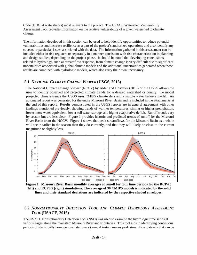
5.1 NATIONAL CLIMATE CHANGE VIEWER (USGS, 2013) The National Climate Change Viewer (NCCV) by Alder and Hostetler (2013) of the USGS allows the user to identify observed and projected climate trends for a desired watershed or county. To model projected climate trends the USGS uses CMIP5 climate data and a simple water balance model. An automated report was generated for the entire Missouri River Basin and is included in the attachments at the end of this report. Results demonstrated in the USGS reports are in general agreement with other findings mentioned previously, showing trends of warmer temperatures, similar or higher precipitation, lower snow water equivalent, lower soil water storage, and higher evaporative deficit. Runoff trends vary by season but are less clear. Figure 1 provides historic and predicted trends of runoff for the Missouri River Basin from the NCCV. Figure 1 shows that peak streamflows for the Missouri Basin as a whole will occur earlier in the season than they do currently, and that they will likely be close to the current magnitude or slightly less.

Figure 1. Missouri River Basin monthly averages of runoff for four time periods for the RCP4.5 (left) and RCP8.5 (right) simulations. The average of 30 CMIP5 models is indicated by the solid

lines and their standard deviations are indicated by the respective shaded envelopes.

5.2 NONSTATIONARITY DETECTION TOOL AND CLIMATE HYDROLOGY ASSESSMENT TOOL (USACE, 2016)

The USACE Nonstationarity Detection Tool (NSD) was used to examine the hydrologic time series at various gages along the mainstem Missouri River and tributaries. This tool aids in identifying continuous periods of statistically homogenous (stationary) annual instantaneous peak streamflow datasets that can be

Draft - 15

adopted for further analysis. Although targeted at Ecosystem restoration, the proposed alternatives for this study require additional planned releases that could potentially increase the odds of downstream flooding if an unexpected precipitation event occurs immediately after the planned release is made. For this reason, peak flow trends provided for use in the USACE tools were considered relevant to the climate change analysis, even though alternatives were comparatively analyzed using daily data time series. In general, gages along the Missouri River between Garrison Dam and Omaha showed nonstationarities. Decisions were made on what period of record to analyze in the tools on a case by case basis for each location (similar to the Green River basin in Ohio example from the Climate Change ECB), in order to have a statistically homogenous data set appropriate for hydrologic analyses. Mainstem gages downstream of Omaha generally didn’t show nonstationarity since they were far enough downstream that the impacts from regulation of the six major mainstem dams were less significant. The NSD tool facilitates access to USGS instantaneous annual peak streamflow records, but does not allow the user to input their own records. The NSD output plots show breaks in the data records that represent nonstationarity, so that the user may select an appropriate period of record resulting in homogenous data to be used in subsequent hydrologic analyses on current and future trends. The breaks in data are called change points, and a “strong” change point is a year in which a nonstationarity was detected for multiple statistical properties (mean, variance, or overall distribution) and/or by multiple test methods. User judgement is required when determining if a change point should be considered “strong” or not. For “strong” change points, the post-change point period of record was checked against the entire period of record using the Monotonic Trend analysis tab within the Nonstationarity Detection Tool. The period of record used for analysis was also adjusted to remove periods of missing data. The USACE Climate Hydrology Assessment Tool detects trends in observed annual maximum daily flow from the selected USGS gage, as well as projected future trends in annual maximum monthly flow for the selected HUC-4 watershed. This tool only allows the user access to preselected data, and does not allow the user to input their own data sets. However, the user can adjust the period of record used by the tool to develop the observed and projected trendlines. For gage sites impacted by regulation, only the period of record after the construction of the most recent water management structure is used to carry out analysis. The projected trendline analysis uses unregulated datasets for the HUC-4 watersheds, whereas the current trendline analysis based on historic gaged data uses datasets which may reflect the impact of upstream regulation. The trendlines generated by the tool for both observed and projected streamflow provide p-values to determine an indication of significance. Based on guidance in the Climate Change ECB, p-values less than 0.05 indicate statistical significance. Many of the sites within the study area are impacted by upstream regulation. The impacts of regulation can cause nonstationarities in an annual peak streamflow record. For this reason, it is preferable to use a naturalized flow record to assess nonstationarities caused by other drivers like distributed land use changes or anthropogenic climate change. At this time, the Nonstationarity Detection tool is only setup to analyze gaged streamflow records and is unable to evaluate time series input by the user. Experts within the USACE Climate Change Community of Practice have the ability to apply the statistical tests applied by the Nonstationarity Detection tool using the R statistical software package. Unfortunately, the time and funding provided for this climate change assessment did not allow for sending datasets out to be analyzed in the tools externally by another party. The tools were used with the available datasets provided within them. Various locations covering mainstem and tributary gages throughout the Missouri River basin were selected to provide a broad-scale summary of the entire basin. Locations were selected from the upper, middle, and lower portions of the Missouri River basin. Tributaries examined included the Niobrara, Nishnabotna, James, Platte, Yellowstone, and Kansas Rivers. Results from the locations are summarized and presented in the following sections.

Draft - 16

5.2.1 Missouri River at Rulo

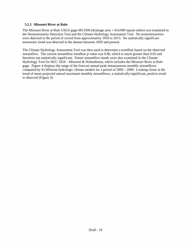
The Missouri River at Rulo USGS gage 6813500 (drainage area = 414,900 square miles) was examined in the Nonstationarity Detection Tool and the Climate Hydrology Assessment Tool. No nonstationarities were detected in the period of record from approximately 1950 to 2015. No statistically significant monotonic trend was detected in the dataset between 1950 and present. The Climate Hydrology Assessment Tool was then used to determine a trendline based on the observed streamflow. The current streamflow trendline p-value was 0.86, which is much greater than 0.05 and therefore not statistically significant. Future streamflow trends were also examined in the Climate Hydrology Tool for HUC 1024 – Missouri & Nishnabotna, which includes the Missouri River at Rulo gage. Figure 4 displays the range of the forecast annual peak instantaneous monthly streamflows computed by 93 different hydrologic climate models for a period of 2000 – 2099. Looking closer at the trend of mean projected annual maximum monthly streamflows, a statistically-significant, positive trend is observed (Figure 5).

Draft - 17

Figure 2. NSD Results for the Missouri River at Rulo.

Draft - 18

Figure 3. Current Streamflow Trend for Missouri River at Rulo, p=0.86.

Figure 4. Projected Annual Maximum Monthly Streamflow for HUC 1024 Missouri –

Nishnabotna.

Draft - 19

Figure 5. HUC 1024 Missouri – Nishnabotna, Mean of Projected Maximum Monthly Streamflow, p

< 0.0001.

5.2.2 Missouri River at Hermann

The Missouri River at Hermann USGS gage 6934500 (drainage area = 522,500 square miles) showed no nonstationarities after the missing data years were removed from the period of record. The full period of record is 1844 to 2015, but the dataset is not continuous. The continuous portion of the period of record starts in 1956. No monotonic trend was detected in the dataset between 1956 and present. The Climate Hydrology Assessment Tool was then used to determine a trendline based on the observed streamflow record. The tool showed no current streamflow trend and a p-value of 0.82, which is larger than 0.05 and therefore not statistically significant. Future streamflow trends were also examined in the Climate Hydrology Tool for HUC 1030 – Lower Missouri. Figure 8 displays the range of the forecast annual peak instantaneous monthly streamflows computed by 93 different hydrologic climate models for a period of 2000 – 2099. Looking closer at the trend of mean projected annual maximum monthly streamflows, a statistically-significant, positive trend is observed (Figure 9).

Draft - 20

Figure 6. NSD Results for the Missouri River at Hermann.

Draft - 21

Figure 7. Current Streamflow Trend for Missouri River at Hermann, p=0.82.

Figure 8. Projected Annual Maximum Monthly Streamflow for HUC 1030 Lower Missouri.

Draft - 22

Figure 9. HUC 1030 Lower Missouri, Mean of Projected Maximum Monthly Streamflow, p <

0.0001.

5.2.3 Yellowstone River at Billings

The Yellowstone River at Billings USGS gage 6214500 (contributing drainage area = 11,414 square miles) showed several nonstationarities, however none of them were considered “strong” since they were only detected by one method: the Bayesian Changepoint Test. The Bayesian Changepoint test is based on the assumption that the data it is being applied to fits a normal distribution. Flow data can rarely be characterized using a normal distribution. Data is available for the Yellowstone River at Billings between 1904 and present, but the continuous portion of the period of record only starts in 1933. No monotonic trend was detected in the dataset between 1933 and present. The Climate Hydrology Assessment Tool was then used to determine a trendline based on the observed streamflow record. The tool showed no current streamflow trend and a p-value of 0.36, which is larger than 0.05 and therefore not statistically significant. Future streamflow trends were also examined in the Climate Hydrology Tool for HUC 1007 – Upper Yellowstone. Figure 12 displays the range of the forecast annual peak instantaneous monthly streamflows computed by 93 different hydrologic climate models for a period of 2000 – 2099. Looking closer at the trend of mean projected annual maximum monthly streamflows, a statistically-significant, positive trend is observed (Figure 13).

Draft - 23

Figure 10. NSD Results for the Yellowstone River at Billings.

Draft - 24

Figure 11. Current Streamflow Trend for Yellowstone River at Billings, p=0.36.

Figure 12. Projected Annual Maximum Monthly Streamflow for HUC 1007 Upper Yellowstone.

Draft - 25

Figure 13. HUC 1007 Upper Yellowstone, Mean of Projected Maximum Monthly Streamflow, p <

0.0001.

5.2.4 James River at LaMoure

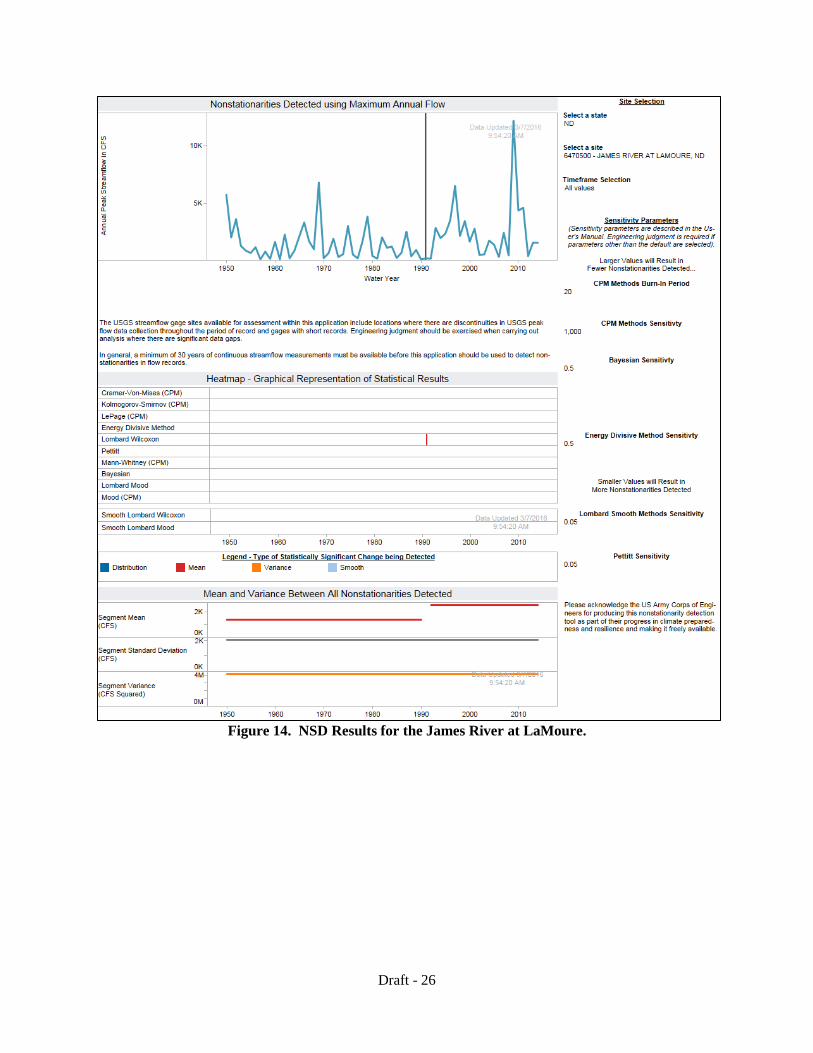
The James River at LaMoure USGS gage 6470500 (contributing drainage area = 1,790 square miles) showed one nonstationarity around 1991, detected for one statistic type (sample mean) by one statistical test, so the changepoint was not considered “strong”. Although Jamestown (constructed in 1953) and Pipestem (constructed in 1973) Reservoirs are known to have an impact on peak streamflows at this gage site, they do not appear to have an impact on the stationarity of the streamflow record. It is possible that they are weakening the signal associated with a nonstationarity caused by another driver like distributed land use changes or anthropogenic climate change. No monotonic trend was detected in the dataset between 1950 and current. The Climate Hydrology Assessment Tool was then used to determine a trendline based on the observed streamflow record. The tool showed no current streamflow trend and a p-value of 0.18, which is larger than 0.05 and therefore not statistically significant. Future streamflow trends were also examined in the Climate Hydrology Tool for HUC 1016 – James. Figure 16 displays the range of the forecast annual peak instantaneous monthly streamflows computed by 93 different hydrologic climate models for a period of 2000 – 2099. Looking closer at the trend of mean projected annual maximum monthly streamflows, a statistically-significant, positive trend is observed (Figure 17).

Draft - 26

Figure 14. NSD Results for the James River at LaMoure.

Draft - 27

Figure 15. Current Streamflow Trend for the James River at LaMoure, p=0.18.

Figure 16. Projected Annual Maximum Monthly Streamflow for HUC 1016 James.

Draft - 28

Figure 17. HUC 1016 James, Mean of Projected Maximum Monthly Streamflow, p < 0.0001.

5.2.5 Niobrara River at Sparks

The Niobrara River at Sparks USGS gage 6461500 (drainage area = 7,150 square miles) showed several nonstationarities. This location is impacted by regulation from Box Butte Dam (1946) on the Niobrara River and Merritt Dam (1964) on the Snake River, both of which have no flood control storage and are mainly irrigation/recreation projects. Two “strong” changepoints were detected by the nonstationarity detection tool, in 1964 and 1984. A statistically significant monotonic trend exists in the dataset when the entire period of record is used for analysis. No statistically significant monotonic trends were detected when the period of record was shifted after 1984, when the most recent “strong” change point was detected. The most recent “strong” changepoint is not associated with any water management project in the basin. It could be caused by land use changes or anthropogenic climate change, but the cause is not known for certain. Because both Box Butte Dam and Merritt Dam are not operated for flood control, it is unlikely that they impact flood peaks. The Climate Hydrology Assessment Tool was then used to determine a trendline based on the entire period of record. The tool showed a negative current streamflow trend and a p-value of less than 0.0001, which is smaller than 0.05 and therefore statistically significant, when the entire period of record was analyzed. Future streamflow trends were also examined in the Climate Hydrology Tool for HUC 1015 – Niobrara. Figure 20 displays the range of the forecast annual peak instantaneous monthly streamflows computed by 93 different hydrologic climate models for a period of 2000 – 2099. Looking closer at the trend of mean projected annual maximum monthly streamflows, a statistically-significant, positive trend is observed (Figure 21).

Draft - 29

Figure 18. NSD Results for the Niobrara River near Sparks.

Draft - 30

Figure 19. Current Streamflow Trend for the Niobrara near Sparks, p<0.0001.

Figure 20. Projected Annual Maximum Monthly Streamflow for HUC 1015 Niobrara.

Draft - 31

Figure 21. HUC 1015 Niobrara, Mean of Projected Maximum Monthly Streamflow, p < 0.0001.

5.2.6 Platte River at Louisville

The Platte River at Louisville USGS gage 6805500 (contributing drainage area = 71,000 square miles) had no nonstationarities. No monotonic trend was detected in the dataset between 1953 and current. The Climate Hydrology Assessment Tool was then used to determine a trendline based on the observed streamflow record. No current streamflow trend was found with a p-value of 0.69, which is greater than 0.05 and therefore not statistically significant. Future streamflow trends were also examined in the Climate Hydrology Tool for HUC 1020 – Platte. Figure 24 displays the range of the forecast annual peak instantaneous monthly streamflows computed by 93 different hydrologic climate models for a period of 2000 – 2099. Looking closer at the trend of mean projected annual maximum monthly streamflows, a statistically-significant, positive trend is observed (Figure 25).

Draft - 32

Figure 22. NSD Results for the Platte River at Louisville.

Draft - 33

Figure 23. Current Streamflow Trend for the Platte River at Louisville, p=0.69.

Figure 24. Projected Annual Maximum Monthly Streamflow for HUC 1020 Platte.

Draft - 34

Figure 25. HUC 1020 Platte, Mean of Projected Maximum Monthly Streamflow, p < 0.0001.

5.2.7 Nishnabotna River above Hamburg

The Nishnabotna River above Hamburg USGS gage 6810000 (drainage area = 2,806 square miles) had several nonstationarities identified. The period of record for this gage is 1917 to 2015, but the continuous portion of the record only starts in 1930. 1935 is the only “strong” changepoint because there is consensus between different statistical tests for this year. No statistically significant monotonic trend was found for the period of record after 1935. It should be mentioned there are no significant reservoirs or diversions in the Nishnabotna basin, but backwater effects are sometimes present at the Hamburg gage due to levees in the area. It is not known for certain what caused the 1935 changepoint. The Climate Hydrology Assessment Tool was then used to determine a trendline based on the observed streamflow record. No current streamflow trend was found, with a p-value of 0.79, which is greater than 0.05 and therefore statistically insignificant. Future streamflow trends were also examined in the Climate Hydrology Tool for HUC 1024 – Missouri-Nishnabotna, and were shown previously in Figures 4 and 5. Looking closer at the trend of mean projected annual maximum monthly streamflows, a statistically-significant, positive trend is observed.

Draft - 35

Figure 26. NSD Results for the Nishnabotna River above Hamburg.

Draft - 36

Figure 27. Current Streamflow Trend for the Nishnabotna River above Hamburg, p=0.79.

5.2.8 Kansas River at Topeka

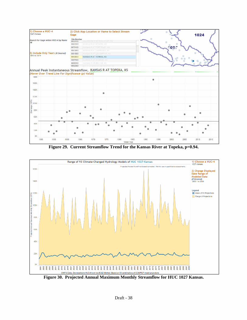
The Kansas River at Topeka USGS gage 6889000 (drainage area = 56,720 square miles) had several nonstationarities. The period of record at this gage is from to 1869 present, but the continuous portion of the dataset only starts in 1902. Three “strong” changepoints detected by multiple statistical tests were identified, around 1930, 1940, and in 1952. No monotonic trend was detected in the dataset when using the entire period of record (1869-2015), the period between “strong” changepoints, or the period after the last “strong” changepoint (1952). Peak streamflow at this location is affected by regulation after 1948, around the time Harlan County Reservoir on the Republican River was constructed. Several other large lakes located upstream of this gage are: Tuttle Creek Lake (1962-flood control), Milford Lake (1962-multipurpose, including flood control), Waconda Lake (1969-flood control and irrigation), and Wilson Lake (1964-flood control). Multiple smaller lakes are also present in the Kansas River system. The Climate Hydrology Assessment Tool was then used to determine a trendline based on the observed streamflow record. No current streamflow trend was found with a p-value of 0.94, which is greater than 0.05 and therefore not statistically significant. Future streamflow trends were also examined in the Climate Hydrology Tool for HUC 1027 – Kansas. Figure 30 displays the range of the forecast annual peak instantaneous monthly streamflows computed by 93 different hydrologic climate models for a period of 2000 – 2099. Looking closer at the trend of mean projected annual maximum monthly streamflows, a statistically-significant, positive trend is observed (Figure 31).

Draft - 37

Figure 28. NSD Results for the Kansas River at Topeka.

Draft - 38

Figure 29. Current Streamflow Trend for the Kansas River at Topeka, p=0.94.

Figure 30. Projected Annual Maximum Monthly Streamflow for HUC 1027 Kansas.

Draft - 39

Figure 31. HUC 1027 Kansas, Mean of Projected Maximum Monthly Streamflow, p = 0.0002369.

5.2.9 Summary of Results

In summary, results for current trends varied, but the majority of results showed no statistically significant trends within the observed historic record. However, all future projected trends for the Missouri River basin at sites examined using the Climate Hydrology Assessment Tool show statistically significant increasing streamflow trends. Some caveats and limitations to the Climate Hydrology Assessment Tool that should be mentioned are: data analyzed should be non-regulated or naturalized to be comparable to the projected hydrology assessment which is based on the unregulated condition. At this time, the tool does not provide the user with an option to enter their own naturalized datasets. Future projections are limited to a HUC-4 scale, and can’t be broken down into specific gage locations.

Draft - 40

5.3 WATERSHED VULNERABILITY ASSESSMENT TOOL (USACE, 2016) The Watershed Vulnerability Assessment (WVA) Tool developed by USACE analyzes 8 business lines for two scenarios (dry and wet) over two epochs (2050 and 2085). The tool enables vulnerability assessment for each USACE business line within each HUC4 watershed across the United States. The vulnerability assessment analysis focuses on the business line(s) and indicator(s) relevant to the project purpose. The WVA tool provides for a screen level assessment of relative vulnerability. The tool flags watersheds as vulnerable across a specific business line if their vulnerability score is in the top 20% of scores computed for the other 202 HUC-4 watersheds in the United States. This tool was used to determine which HUCs in the entire Missouri River watershed for both wet and dry scenarios in both 2050 and 2085 epochs have flood risk reduction business line vulnerabilities and/or ecosystem restoration business line vulnerabilities. The other business lines that can be examined using the Watershed Vulnerability Assessment Tool are navigation, hydropower, recreation, water supply, regulatory, and emergency management.

5.3.1 Flood Risk Reduction

Although targeted at Ecosystem restoration, the proposed alternatives for this study require additional planned releases that could potentially increase the odds of downstream flooding if an unexpected precipitation event occurs immediately after the planned release is made. For this reason, flood risk reduction vulnerabilities were considered applicable to this study. Flood risk reduction vulnerabilities are determined by the tool based on the following five indicators:

• Acres of urban area within the 500-year (0.2% exceedance) floodplain • Coefficient of variation of cumulative annual flow • Streamflow elasticity, or ratio of streamflow response to precipitation • Flood magnification: ratio of 10% exceedance flow in the future to the 10% exceedance flow in

the base flow period, for cumulative monthly flows • Flood magnification: ratio of 10% exceedance flow in the future to the 10% exceedance flow in

the base flow period, for local monthly flows Relative to the other HUC-4 watersheds in the United States, no watersheds within the Northwestern Division Omaha District (NWO) were found to be highly vulnerable for either epoch in the dry scenario. However, flood risk reduction vulnerabilities were found in two Northwestern Division Kansas City District (NWK) Missouri River HUCs (1026-Smoky Hill and 1027-Kansas) for both epochs in the dry scenario. For the wet scenario epochs, flood risk reduction vulnerabilities were found for the following HUCs in the Missouri River basin (9 in NWO and 5 in NWK) shown in Figures 36 and 37. For both the wet and dry scenarios, the results were consistent for the two epochs analyzed by the tool. The Missouri River basin is covered by the Northwestern Division (NWD). Missouri River basins with flood risk reduction vulnerabilities (wet and/or dry) are shown in Figure 38. Different shades of the same color in Figures 36 and 37 represent the different Districts within the same Division. 1008 – Bighorn 1009 – Powder-Tongue 1012 – Cheyenne 1016 – James 1018 – North Platte 1020 – Platte 1021 – Loup 1022 – Elkhorn 1023 – Missouri-Little Sioux

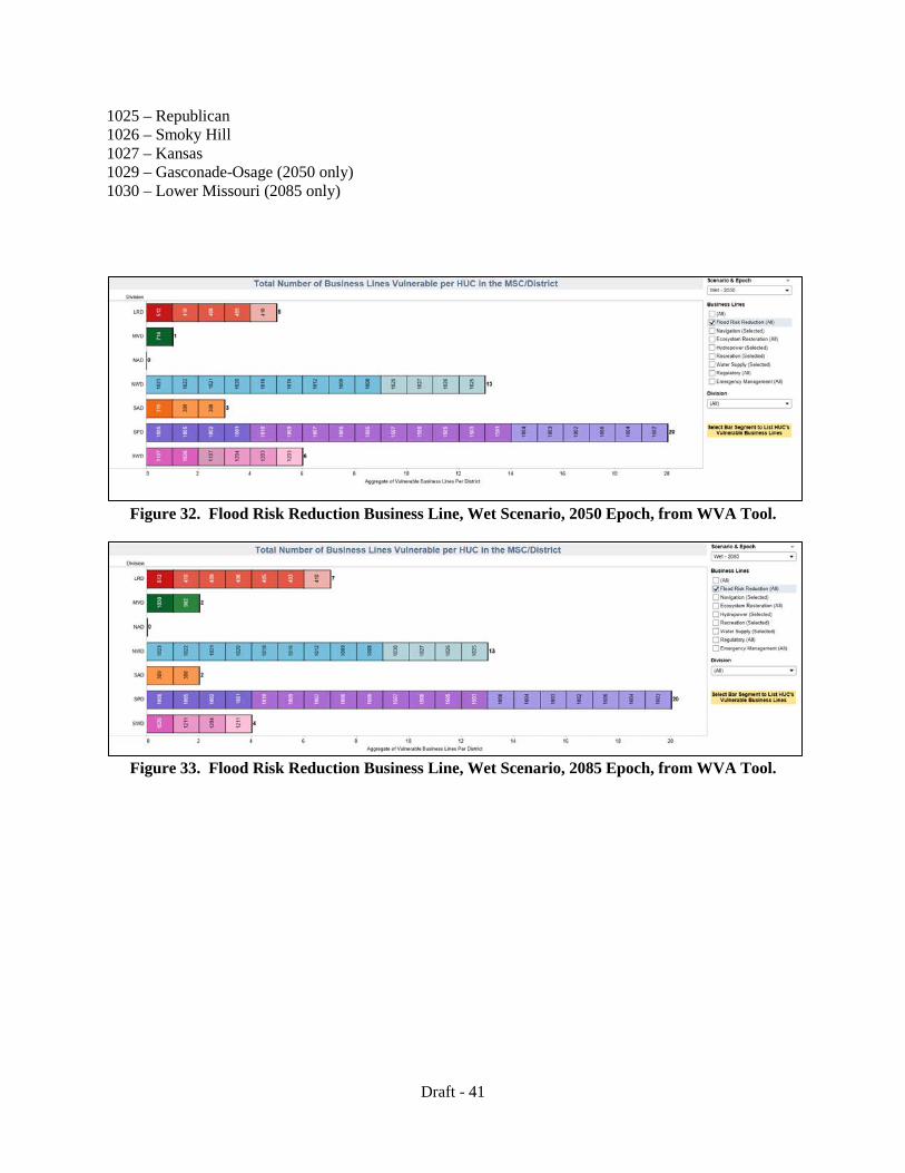
Draft - 41

1025 – Republican 1026 – Smoky Hill 1027 – Kansas 1029 – Gasconade-Osage (2050 only) 1030 – Lower Missouri (2085 only)

Figure 32. Flood Risk Reduction Business Line, Wet Scenario, 2050 Epoch, from WVA Tool.

Figure 33. Flood Risk Reduction Business Line, Wet Scenario, 2085 Epoch, from WVA Tool.

Draft - 42

Figure 34. HUC-4 Missouri River Basins with Flood Risk Reduction Vulnerabilities.

Draft - 43

5.3.2 Ecosystem Restoration

Since the Missouri River Recovery Management Plan is part of the Missouri River Recovery Program (MRRP), which is the umbrella program that works to coordinate activities on the Missouri River for restoration of native habitats and to comply with the Endangered Species Act and 2003 Biological Opinion, the ecosystem restoration business lines were also reviewed. Ecosystem restoration vulnerabilities are determined by the tool based on the following nine indicators:

• Percentage of riparian and wetland plant communities that are at risk of extinction, based on remaining number and condition, remaining acreage, threat severity, etc

• Mean runoff: average annual runoff, excluding upstream freshwater inputs • Sediment elasticity, or ratio of future to present sediment load • Coefficient of variation of cumulative monthly flow • Streamflow elasticity, or ratio of streamflow response to precipitation • Macroinvertebrate index of biotic condition • Flood magnification: ratio of 10% exceedance flow in the future to the 10% exceedance flow in

the base flow period, for cumulative monthly flows • Flood magnification: ratio of 10% exceedance flow in the future to the 10% exceedance flow in

the base flow period, for local monthly flows • Low flow reduction: ratio of the 90% exceedance flow in the future to the 90% exceedance flow

in the base flow period, for cumulative monthly flows For the dry scenario in both epochs, ecosystem restoration vulnerabilities were identified in the following Missouri River basin HUCs (Figures 39 and 40): 1006 – Missouri-Poplar 1018 – North Platte 1022 – Elkhorn 1026 – Smoky Hill 1027 – Kansas 1028 – Chariton-Grand 1029 – Gasconade-Osage 1404 – Great Divide-Upper Green

Figure 35. Ecosystem Restoration Business Line, Dry Scenario, 2050 Epoch, from WVA Tool.

Draft - 44

Figure 36. Ecosystem Restoration Business Line, Dry Scenario, 2085 Epoch, from WVA Tool.

For the wet scenario, ecosystem restoration vulnerabilities were identified in the following Missouri River basin HUCs (Figures 41 and 42): 1006 – Missouri-Poplar 1008 – Big Horn 1009 – Powder-Tongue 1012 – Cheyenne 1015 – Niobrara 1018 – North Platte 1021 – Loup (2085 only) 1022 – Elkhorn 1025 – Republican 1026 – Smoky Hill 1027 – Kansas 1029 – Gasconade-Osage 1404 – Great Divide-Upper Green

Figure 37. Ecosystem Restoration Business Line, Wet Scenario, 2050 Epoch, from WVA Tool.

Draft - 45

Figure 38. Ecosystem Restoration Business Line, Wet Scenario, 2085 Epoch, from WVA Tool.

Missouri River basins with ecosystem vulnerabilities, for wet and/or dry scenarios, are shown in Figure 43.

Draft - 46

Figure 39. HUC-4 Missouri River Basins with Ecosystem Restoration Vulnerabilities.

Draft - 47

5.3.3 Summary of Results

The results show that the Missouri River basin will continue to have flood risk reduction and ecosystem restoration vulnerabilities across the 21st Century, with higher vulnerability under wetter future scenarios. This information should be used to increase resiliency of proposed project alternatives and reduce vulnerabilities.

6 CLIMATE CHANGE EFFECTS ON STUDY ALTERNATIVES

6.1 ALTERNATIVES SUMMARY Climate change has the potential to impact various hydrologic parameters. The changing hydrologic parameters could, in turn, have impacts on the various alternatives being assessed as part of this study. This section provides an overview of the alternatives. The alternatives being considered for this study were not developed with climate change in mind, but the final implemented alternative should be adaptive to allow for mitigating the potential effects of climate change. The Missouri River Recovery Management Plan currently has 6 alternatives left that are being considered. They are: Alt1a_NoAction, Alt2a_BiOp, Alt3a_Mech, Alt4a_Spring2-42MAF, Alt5a_Fall5-35SL, and Alt6a_SpawningCue. The alternatives are summarized below, and additional detailed information is provided in the main report.

6.1.1 Alt1a_NoAction

• Operations are closely based on current Master Manual criteria • Local inflows are adjusted by the difference between the historic and present level depletions to

ensure period-of-record datasets are homogeneous and reflect current water use. • Flood targets are as outlined in the Master Manual • Reservoir storages are based on current reservoir surveys • Uses all four navigation target locations when setting navigation releases • Balance System storage by March 1 • Plenary bimodal spawning cue pulse attempted each year

o March Spawning Cue System storage preclude is 40.0 MAF on March 1 Rise begins the day after releases achieve the flow required for navigation Peak pulse is 5 kcfs minus the contribution of the James River Rate of rise is 5 kcfs for one day Total Gavins Point release will not exceed 35 kcfs (power plant capacity) Maintain peak for 2 days Releases reduced over the 5 days until flow-to-target navigation releases are

reached o May Spawning Cue

System storage preclude is 40.0 MAF on May 1 Rise begins on May 1 Peak is 2 prorated amounts resulting in a range of 9 – 20 kcfs

• First prorated amount is based on a linear interpolation from 12-16 kcfs based on System storages between 40.0-54.5 MAF. No greater than 16 kcfs.

Draft - 48

• The second prorated amount is further adjusted based on the calendar year runoff forecast above Gavins Point: linear interpolation from 0-25% increase based on forecasts between median and upper quartile; linear interpolation from 0-25% decrease based on forecasts between median and lower quartile

Rate of rise is 6 kcfs per day Total Gavins Point release is not limited by power plant capacity Maintain peak for 2 days Releases reduced by 30% for the first 2 days followed by a proportional

reduction in releases back to navigation releases over 8 days o Downstream Flood Targets

Omaha = 41 kcfs Nebraska City = 47 kcfs Kansas City = 71 kcfs Pulse is reduced by 500 cfs increments until flood targets are no longer exceeded

or until the pulse magnitude is 0 o Based on ResSim POR simulations, Gavins Point releases during the March spawning

cue ranged from 22-35 kcfs. Gavins Point releases during the May spawning cue ranged from 25-41 kcfs.

6.1.2 Alt2a_BiOp

• Plenary bimodal spawning cue pulse that is specified in the Master Manual is not included • Uses all four navigation target locations when setting navigation releases • If “no service” is determined on March 15, GAPT releases are to be determined based on meeting

water supply targets until the winter season; first and second pulses will not be carried out. • Max winter GAPT release: 16 kcfs • Alternative 2 spawning cue pulse attempted each year. Pulse is not started or terminated

whenever flood targets are exceeded. o March Spawning Cue

System storage preclude is 40.0 MAF on March 1 Rise begins with normal increase for navigation releases (around March 15) Peak is 31 kcfs total Gavins Point release Proportional increase over 7 days to the peak Maintain peak for 7 days Proportional decrease over 7 days to reach flow-to-target navigation releases Disregard pulse if storage evacuation service level is determined by March 15

assessment o May Spawning Cue

System storage preclude is 40.0 MAF on May 1 Rise begins on May 1 Proportional increase over 7 days to peak

• Note: PAL specifies a proportional increase over 7-10 days but for modeling purposes, 7 days was used

Peak based on March 1 runoff forecast

Draft - 49

• Median = 16 kcfs • Upper quartile or higher runoff = 20 kcfs rise • Lower quartile or lower runoff = 12 kcfs rise • Maximum Gavins Point release is limited to 60 kcfs

Maintain peak for: • 14 days – lower quartile or lower runoff • 25 days – median runoff • 35 days – upper quartile or higher runoff

Descending limb not less than 7 days Flood control constraints

• Add pulse magnitude to the current USACE flood control constraints outlined in Tables VII-7 and VII-8 in master manual

o Based on ResSim POR simulations, Gavins Point releases during the March spawning cue were 31 kcfs. Gavins Point releases during the May spawning cue ranged from 38-56 kcfs.

• End of second pulse to June 23: return to “steady release” scenario to specify Gavins Point releases; if steady releases from Gavins Point are lower than 25 kcfs, stay on the steady release level until the summer low flow reduction to 21 kcfs.

• Summer Low Flows o Summer low flows are only implemented in the following two years after complete

March and May spawning cues o June 23rd to July 1

25 kcfs GAPT release o July 1: Assess navigation season length

If there is a shortened navigation season as determined by the Master Manual • GAPT releases are to be determined based on meeting water supply

targets (open channel non-navigation season) • The duration of those releases is equivalent to that of the number of days

the season is shortened less the 8 days in June (eg. if season is shortened 30 days, GAPT releases are for water supply for 22 days starting July 1)

• Following that duration, set flow to 25 kcfs until July 15 then drop the release to 21 kcfs until August 15 and then return to 25 kcfs until Sept 1

• FTT operations from Sept 1 until Dec 1 If there is not a shortened navigation season

• Continue 25 kcfs from July 1-July 15 then drop the release to 21 kcfs until August 15 and then return to 25 kcfs until Sept 1

• Flow to target operations from Sept 1 until Dec 1 or Dec 10 if a ten day extension is determined

6.1.3 Alt3a_Mech

• Operations are closely based on current Master Manual criteria o Plenary bimodal spawning cue pulse that is specified in the Master Manual is not

included • Local inflows are adjusted by the difference between the historic and present level depletions to

ensure period-of-record datasets are homogeneous and reflect current water use. • Flood targets are as outlined in the Master Manual • Reservoir storages are based on current reservoir surveys

Draft - 50

• Uses all four navigation target locations when setting navigation releases • Balance System storage by March 1 • Ecosystem restoration projects (ie sandbar habitat) are created by mechanical methods and not by

changes to System regulation.

6.1.4 Alt4a_Spring2-42MAF

• Alternative based on Alt 1 (current operations) but including a high spring release used to create sandbar habitat for the Least Tern and Piping Plover.

• Local inflows are adjusted by the difference between the historic and present level depletions to ensure period-of-record datasets are homogeneous and reflect current water use.

• Plenary bimodal spawning cue pulse that is specified in the Master Manual is not included • Reservoir storages are based on current reservoir surveys • Uses all four navigation target locations when setting navigation releases • Balance System storage by March 1 • ESH Creation Release

o System storage >= 42.0 kcfs on April 1 o Based on EA team’s discharge vs. duration table for 250 ESH, if a monthly averaged

release for the specified duration has not occurred in the past 3 years, releases can occur if first check is met

o Attempts ESH creation release starting April 1 of up to 60 kcfs as often as every 4 years. Duration increases as magnitude is decreased. 60 kcfs requires a duration of 35 days 55 kcfs requires a duration of 49 days 50 kcfs requires a duration of 77 days 45 kcfs requires a duration of 175 days

o Flood targets OMA – 71 kcfs NCNE – 82 kcfs MKC – 126 kcfs

o If flood targets are exceeded, reduce GAPT release by 5 kcfs until flood targets are no longer exceeded If GAPT release falls below 45 kcfs, terminate flow

o Increased releases will be made from GAPT, FTRA, and GARR in the same year FTRA releases will be similar in magnitude to GAPT releases GARR releases will be approximately 17.5 kcfs less than GAPT

o Based on ResSim POR simulations, Gavins Point releases the ESH creation releases ranged between 45-60 kcfs.

• Mechanical habitat creation will be used to reach target habitat acres if flow does not do it alone

6.1.5 Alt5a_Fall5-35SL

• Alternative based on Alt 1 (current operations) but including a high fall release used to create sandbar habitat for the Least Tern and Piping Plover.

Draft - 51

• Local inflows are adjusted by the difference between the historic and present level depletions to ensure period-of-record datasets are homogeneous and reflect current water use.

• Plenary bimodal spawning cue pulse that is specified in the Master Manual is not included • Reservoir storages are based on current reservoir surveys • Uses all four navigation target locations when setting navigation releases • Balance System storage by March 1 • ESH Creation Release

o Service level >= 35.0 kcfs on October 15 o Based on EA team’s discharge vs. duration table for 250 ESH, if a monthly averaged

release for the specified duration has not occurred in the past 3 years, releases can occur if first check is met

o Attempts ESH creation release starting October 15 of up to 60 kcfs as often as every 4 years. Duration increases as magnitude is decreased. 60 kcfs requires a duration of 35 days 55 kcfs requires a duration of 49 days 50 kcfs requires a duration of 77 days 45 kcfs requires a duration of 175 days

o Flood targets OMA – 71 kcfs NCNE – 82 kcfs MKC – 126 kcfs

o If flood targets are exceeded, reduce GAPT release by 5 kcfs until flood targets are no longer exceeded If GAPT release falls below 45 kcfs, terminate flow

o Increased releases will be made from GAPT, FTRA, and GARR in the same year FTRA releases will be similar in magnitude to GAPT releases GARR releases will be approximately 17.5 kcfs less than GAPT

o Based on ResSim POR simulations, Gavins Point releases the ESH creation releases ranged between 45-60 kcfs.

• Mechanical habitat creation will be used to reach target habitat acres if flow does not do it alone

6.1.6 Alt6a_SpawningCue

• Alternative based on Alt 1 (current operations) but including a high spring release used as a spawning cue for the Pallid Sturgeon.

• Local inflows are adjusted by the difference between the historic and present level depletions to ensure period-of-record datasets are homogeneous and reflect current water use.

• Plenary bimodal spawning cue pulse that is specified in the Master Manual is not included • Reservoir storages are based on current reservoir surveys • Uses all four navigation target locations when setting navigation releases • Balance System storage by March 1 • Alternative 6 spawning cue pulse attempted every 3 years. Pulse is not started or terminated

whenever flood targets are exceeded. o March Pulse

Draft - 52

System storage preclude is 40.0 MAF on March 15 Initiate the pulse once navigation releases are met at downstream target locations Increase by 2,200 cfs per day until pulse magnitude is achieved Peak pulse magnitude is equal to the navigation release that occurred on the day

the pulse was initiated • Peak Gavins Point release is double the navigation release that occurred

on the day the pulse was initiated Maintain peak for 2 days Reduce pulse by 1,700 cfs per day until flow-to-target navigation releases are

reached Flood Targets

• Omaha: 41 kcfs + Pulse Magnitude • Nebraska City: 47 kcfs + Pulse Magnitude • Kansas City: 71 kcfs + Pulse Magnitude

o May Pulse Initiate the pulse on May 18

• Note: A varied initiation date based on water temperature was specified in the PAL, but May 18 was used for modeling

Increase by 2,200 cfs per day until pulse magnitude is achieved Peak pulse magnitude is equal to the steady release on May 18

• Peak Gavins Point release is double the steady release that occurred on the day the pulse was initiated

Maintain peak for 2 days Reduce pulse by 1,900 cfs per day until steady release is reached Flood Targets

• Omaha: 41 kcfs + Pulse Magnitude • Nebraska City: 47 kcfs + Pulse Magnitude • Kansas City: 71 kcfs + Pulse Magnitude

o Based on ResSim POR simulations, Gavins Point releases during the March spawning cue were 39-61 kcfs. Gavins Point releases during the May spawning cue ranged from 50-67 kcfs.

Table 6-1 summarizes the changes to the System impacting the hydrology of the study area with regards to the baseline basin condition (Alt 1 – No Action).

Draft - 53

Table 6-1. Alternatives Comparison with Regards to Alternative 1 (No Action).

Alternative March - April May - August September - November December - February

Alt 2 Alt 1 early spring spawning

cue replaced by Alt 2 early spring spawning cue

Alt 1 late spring spawning cue replaced by Alt 2 late spring spawning cue

Low summer flow occur between June 25 and September 1

Navigation season always ends on December 1

Maximum winter release is 16 kcfs

Alt 3 Alt 1 early spring spawning cue removed

Alt 1 late spring spawning cue removed No operational changes No operational changes

Alt 4

Alt 1 early spring spawning cue removed

Alt 4 ESH-creating release from Gavins Point and Garrison

Alt 1 late spring spawning cue removed

Alt 4 ESH-creating release from Gavins Point and Garrison may continue into summer months

No operational changes No operational changes

Alt 5 Alt 1 early spring spawning cue removed

Alt 1 late spring spawning cue removed

Alt 5 ESH-creating release from Gavins Point and Garrison

No operational changes

Alt 6 Alt 1 early spring spawning cue replaced by Alt 6 early spring spawning cue

Alt 1 late spring spawning cue replaced by Alt 6 late spring spawning cue

No operational changes No operational changes

Draft - 54

The daily differences throughout the period-of-record between alternatives and the no action (Alt 1) plan were examined at each reservoir and for the System. Alt 2, Alt 4, Alt 5, and Alt 6 show a trend of lower pool elevations at Fort Peck, Garrison, and Oahe when compared to Alt 1 over the period-of-record due to the ESH-creating or spawning cues in each alternative. Pool elevations at Big Bend, Fort Randall, and Gavins Point remain mostly unchanged as they operate for their respective guide curves. Changes in Fort Peck’s, Garrison’s, and Oahe’s pool elevations closely follow changes in System storage (volume of water in the System). Alt 2, Alt 4, Alt 5, and Alt 6 show a trend of lower System storage for some years on March 1 due to increased releases at other times throughout the year; however Alt 2’s low summer flow and winter release operations conserve water during some years resulting in higher System storage on March 1. These four alternatives result in higher System storage some years, and lower System storage other years. The spawning cues also increase the chance for downstream flooding if they are closely followed by an unanticipated high intensity precipitation event for Alt 2, Alt 4, Alt 5, and Alt 6. Alt 3’s operations have a minimal effect on System storage as all of the changes are within ±0.5 MAF. Alt 3 allows the most flexibility for reservoir managers in deciding operations, by not imposing any new flow requirements.

6.2 CLIMATE CHANGE CONCLUSIONS USACE climate change literature reviews and most references from other sources for the Missouri River Basin agree that future climate trends are likely to have increased temperatures and precipitation. The USACE climate assessment tool and some other sources point towards increased streamflow trends as well. The USGS NCCV tool points towards earlier timing of peak streamflows for the Missouri River basin, but magnitudes similar to or less than current peak streamflow magnitudes. There is no readily apparent trend in historic streamflow data, and no clear consensus on future streamflow data. The increased temperatures noted in the literature review are likely to result in earlier spring snowmelt, decreased snowmelt season duration, and decreased peak SWE. Increased air temperatures could also have impacts on water temperatures and water quality, which could exacerbate impacts of alternatives with low summer flows. According to the results of the literature review, rainfall events are likely to become even more sporadic for the entire Missouri River basin. Large rain events are likely to become more frequent and interspersed by longer relatively dry periods. The literature review also indicates that sediment loading is expected to increase for at least one Missouri River reservoir in the basin, also adding to regulation challenges and impacting alternatives. The results of the vulnerability assessment point to an increase in potential flood risk reduction vulnerabilities for some sub-watersheds in the basin for future years. The vulnerability assessment also indicates that in the future there will be an increase in the potential for habitat degradation for some sub-watersheds in the basin. Consequently, projects like the Missouri River Recovery Management Plan, which is aimed at the restoration of native habitats and the application of adaptive management practices, are integral to building resiliency into our systems to prevent further degradation of natural habitat. Extremes in climate will magnify periods of wet or dry weather resulting in longer, more severe droughts, and larger, more extensive flooding. These increased sporadic flood and drought periods could prove challenging for reservoir regulation, and have impacts to all the proposed alternatives summarized previously. The sporadic flooding would increase the risk of downstream flooding during periods of pulse releases. Climate change consequences with regards to the various proposed alternatives are summarized in the following table. Based on the results summarized previously and the following table, Alternative 3 would be the best option with regards to dealing with potential climate change impacts.

Draft - 55

Alternative 3 provides the least change to the existing System, and allows reservoir management the most flexibility with regards to releases and handling excesses or shortages in System storage. Alternative 3 is recommended so that flexibility can be built in to the System to help mitigate uncertainty and variability from future climate change trends.

Draft - 56

Table 6-2. Climate Change Consequences to Alternatives Matrix.

Alternative

Expected Climate Change Variable

Increased Air Temperature Increased Precipitation & Streamflow

Decreased Peak Snow Water Equivalent

Earlier Snowmelt Date & Decreased Snow Accumulation

Season Duration Increased Sedimentation* Increased Sporadicalness of

Floods & Droughts

Alt1a_NoAction

• During summer water supply operations, could potentially have WQ issues with

lower Gavins Point releases if water temperature increases.

• May be able to run spring pulses more often due to increased system storage.

• Forecasting calendar year runoff has the potential to become less accurate, since

forecasting runoff based on precipitation is much more difficult than forecasting

runoff based on SWE.

• May be able to run spring pulses more frequently due to System storage rising

earlier in the year.

• Decreased System storage may lead to decreased frequency of all pulses

(assuming pulse requirements remain the same and sedimentation is not addressed).

• Accuracy of downstream forecasting may decrease, resulting in more frequent

flood impacts caused by pulses.

• However, the frequency of a completed

pulse will likely decrease due to exceeding flood targets more frequently.

• Less accurate forecasts may result in an increased risk of overall System impacts (ie lower reservoir elevations, lower SL, etc) due to setting pulse magnitude too

high.

• Could potentially lower the SL for 2nd half of navigation season if current year's

runoff falls as rain in late winter while System storage is being evacuated back to

56.1 MAF.

• Have a greater potential to impact System storage with pulses if more

droughts occur.

Alt2a_BiOp

• During summer water supply operations, could potentially have WQ issues with

lower Gavins Point releases if water temperature increases.

• May be able to run spring pulses more often due to increased system storage.

• Forecasting calendar year runoff has the potential to become less accurate, since

forecasting runoff based on precipitation is much more difficult than forecasting

runoff based on SWE.

• May be able to run spring pulses more frequently due to System storage rising

earlier in the year.

• Decreased System storage may lead to decreased frequency of all pulses

(assuming pulse requirements remain the same and sedimentation is not addressed).

• Accuracy of downstream forecasting may decrease, resulting in more frequent

flood impacts caused by pulses.

• However, the frequency of a completed

pulse will likely decrease due to exceeding flood targets more frequently.

• Less accurate forecasts may result in an increased risk of overall System impacts (ie lower reservoir elevations, lower SL, etc) due to setting pulse magnitude too

high.

• Could potentially lower the SL for 2nd half of navigation season if current year's

runoff falls as rain in late winter while System storage is being evacuated back to

56.1 MAF.

• Have a greater potential to impact System storage with pulses if more

droughts occur.

Alt3a_Mech • During summer water supply operations,

could potentially have WQ issues with lower Gavins Point releases if water

temperature increases.

• Could potentially lower the SL for 2nd half of navigation season if current year's

runoff falls as rain in late winter while System storage is being evacuated back to

56.1 MAF.

Alt4a_Spring2-42MAF

• During summer water supply operations, could potentially have WQ issues with

lower Gavins Point releases if water temperature increases.

• May be able to run ESH creation releases more often due to increased

system storage.

• May be able to run ESH creation releases more frequently due to System storage

rising earlier in the year.

• Decreased System storage may lead to decreased frequency of all ESH creation releases (assuming release requirements

remain the same and sedimentation is not addressed).

• Accuracy of downstream forecasting may decrease, resulting in more frequent

flood impacts caused by ESH creation releases.

• However, the frequency of a completed ESH creation release will likely decrease

due to exceeding flood targets more frequently.

• Could potentially lower the SL for 2nd half of navigation season if current year's

runoff falls as rain in late winter while System storage is being evacuated back to

56.1 MAF.

• Have a greater potential to impact

System storage with ESH creation releases if more droughts occur.

Alt5a_Fall5-35SL

• During summer water supply operations, could potentially have WQ issues with

lower Gavins Point releases if water temperature increases.

• May be able to run ESH creation releases more often due to increased

system storage.

• May be able to run ESH creation releases less frequently if SL is lowered for 2nd half

of navigation season.

• Decreased System storage may lead to decreased frequency of all ESH creation releases (assuming release requirements

remain the same and sedimentation is not addressed).

• Accuracy of downstream forecasting may decrease, resulting in more frequent

flood impacts caused by ESH creation releases.

• However, the frequency of a completed ESH creation release will likely decrease

due to exceeding flood targets more frequently.

• Could potentially lower the SL for 2nd half of navigation season if current year's

runoff falls as rain in late winter while System storage is being evacuated back to

56.1 MAF.

• Have a greater potential to impact

System storage with ESH creation releases if more droughts occur.

Alt6a_SpawningCue

• During summer water supply operations, could potentially have WQ issues with

lower Gavins Point releases if water temperature increases.

• May be able to run spring spawning cues more often due to increased system

storage.

• May be able to run spring spawning cues more frequently due to System storage

rising earlier in the year.

• Decreased System storage may lead to decreased frequency of all spawning cues

(assuming spawning cue requirements remain the same and sedimentation is not

addressed).

• Accuracy of downstream forecasting may decrease, resulting in more frequent flood impacts caused by spawning cues.

• May spawning cue might be initiated earlier if temperature is used to determine

start date.

• However, the frequency of a completed spawning cue will likely decrease due to exceeding flood targets more frequently.

• Could potentially lower the SL for 2nd half of navigation season if current year's

runoff falls as rain in late winter while System storage is being evacuated back to

56.1 MAF.

• Have a greater potential to impact

System storage with spawning cues if more droughts occur.

*Reference for this variable is 1 large reservoir in the Upper basin. System storage is the total volume of water in the System.

Draft - 57

7 REFERENCES

Cayan, D. R., S. A. Kammerdiener, M. D. Dettinger, J. M. Caprio, and D. H. Peterson. 2001. “Changes in the Onset of Spring in the Western U.S.” Bulletin of the American Meteorology Society 82(3):399-415.

Gutowski, W.J., et al. 2008. Causes of Observed Changes in Extremes and Projections of Future Changes in Weather and Climate Extremes in a Changing Climate.

Janetos, A., L. Hansen, D. Inouye, B.P. Kelly, L. Meyerson, B. Peterson, and R. Shaw. 2008. “Biodiversity.” The effects of climate change on agriculture, land resources, water resources, and biodiversity in the U.S. A report by the U.S. Climate Change Science Program and the subcommittee on Global Change Research. Washington, DC. 362 pp.

Lettenmaier, D.P., A.W. Wood, R.N. Palmer, E.F. Wood, and E.Z. Stakhiv. 1999. “Water Resources Implications of Global Warming: A U.S. Regional Perspective.” Climate Change 43(3):537-79.

NOAA, Jan. 2013. Technical Report NESDIS 142-4: Regional Climate Trends and Scenarios for the US National Climate Assessment, Part 4. Climate of the US Great Plains.

Qiao, Lei, Zaitao Pan, Robert B. Herrmann, and Yang Hong. 2013. “Hydrological Variability and

Uncertainty of Lower Missouri River Basin Under Changing Climate.” Journal of the American Water Resources Association (JAWRA) 12126:1-15.

Stewart, I. T., D. R. Cayan, and M. D. Dettinger. 2005. “Changes Toward Earlier Streamflow Timing Across Western North America”. Journal of Climate, 18: 1136-55.

USACE-CEMVR, Sept. 2012. Climate Change Impacts on the Operation of Coralville Lake, Iowa.

USACE, Sept. 2012. Climate Change Adaptation Pilots (summary document).

USACE, 2016. Climate Hydrology Assessment Tool. https://maps.crrel.usace.army.mil/apex/f?p=313:2:0::NO

USACE, Spetember 2016. Engineering and Construction Bulletin 2016-25. Subject: Guidance for Climate Change Adaptation Engineering Inputs to Inland Hydrology for Civil Works Studies, Designs, and Projects.

USACE-Institute for Water Resources, January 2015. Recent US Climate Change and Hydrology Literature Applicable to US Army Corps of Engineers Missions, Missouri River Region 10.

USACE-MRBWM, July 2014. Climate Change Evaluation – Upper Missouri River Basin Mountain Snowpack – Accumulation and Runoff.

USACE-MRRPCCC, 03 Feb. 2014. Inclusion of Climate Change within Missouri River Recovery, draft white paper.

Draft - 58

USACE, 2016. Non-Stationarity Detection Tool. https://maps.crrel.usace.army.mil/apex/f?p=257:2:0::NO

USACE-NWO, Sept. 2012. Climate Change Sediment Yield Impacts on Operations Evaluations at Garrison Dam.

USACE, 2016. Watershed Climate Vulnerability Assessment Tool. https://maps.crrel.usace.army.mil/rcc_prod/f?p=763:LOGIN:12716728010988 USBR, Jan. 2011. Technical Memorandum 86-68210-2010-03: Literature Synthesis on Climate Change Implications for Water and Environmental Resources, Second Edition. USBR, Mar. 2011. West-Wide Climate Risk Assessments: Bias-Corrected and Spatially Downscaled Surface Water Projections. USGS, Alder and Hostetler, 2013. National Climate Change Viewer.

Draft - 59

8 ATTACHMENT: USGS CLIMATE CHANGE VIEWER RESULTS

U.S. Geological Survey - National Climate Change Viewer

Summary of Missouri Region (10)

May 12, 2014

SUMMARY OF 10 1 MAXIMUM 2-M AIR TEMPERATURE

1 Maximum 2-m Air Temperature

Figure 1: Seasonal average time series of maximum 2-m air temperature for historical (black), RCP4.5 (blue) and RCP8.5 (red).The historical period ends in 2005 and the future periods begin in 2006. The average of 30 CMIP5 models is indicated by the solidlines and their standard deviations are indicated by the respective shaded envelopes.

Figure 2: Monthly averages of maximum 2-m air temperature for four time periods for the RCP4.5 (left) and RCP8.5 (right)simulations. The average of 30 CMIP5 models is indicated by the solid lines and their standard deviations are indicated by therespective shaded envelopes.

1 -Alder and Hostetler, USGS

SUMMARY OF 10 2 MINIMUM 2-M AIR TEMPERATURE

2 Minimum 2-m Air Temperature

Figure 3: Seasonal average time series of minimum 2-m air temperature for historical (black), RCP4.5 (blue) and RCP8.5 (red).The historical period ends in 2005 and the future periods begin in 2006. The average of 30 CMIP5 models is indicated by the solidlines and their standard deviations are indicated by the respective shaded envelopes.

Figure 4: Monthly averages of minimum 2-m air temperature for four time periods for the RCP4.5 (left) and RCP8.5 (right)simulations. The average of 30 CMIP5 models is indicated by the solid lines and their standard deviations are indicated by therespective shaded envelopes.

2 -Alder and Hostetler, USGS

SUMMARY OF 10 3 PRECIPITATION

3 Precipitation

Figure 5: Seasonal average time series of precipitation for historical (black), RCP4.5 (blue) and RCP8.5 (red). The historicalperiod ends in 2005 and the future periods begin in 2006. The average of 30 CMIP5 models is indicated by the solid lines andtheir standard deviations are indicated by the respective shaded envelopes.

Figure 6: Monthly averages of precipitation for four time periods for the RCP4.5 (left) and RCP8.5 (right) simulations. The averageof 30 CMIP5 models is indicated by the solid lines and their standard deviations are indicated by the respective shaded envelopes.

3 -Alder and Hostetler, USGS

SUMMARY OF 10 4 SNOW WATER EQUIVALENT

4 Snow Water Equivalent

Figure 7: Seasonal average time series of snow water equivalent for historical (black), RCP4.5 (blue) and RCP8.5 (red). Thehistorical period ends in 2005 and the future periods begin in 2006. The average of 30 CMIP5 models is indicated by the solidlines and their standard deviations are indicated by the respective shaded envelopes.

Figure 8: Monthly averages of snow water equivalent for four time periods for the RCP4.5 (left) and RCP8.5 (right) simulations.The average of 30 CMIP5 models is indicated by the solid lines and their standard deviations are indicated by the respective shadedenvelopes.

4 -Alder and Hostetler, USGS

SUMMARY OF 10 5 RUNOFF

5 Runoff

Figure 9: Seasonal average time series of runoff for historical (black), RCP4.5 (blue) and RCP8.5 (red). The historical period endsin 2005 and the future periods begin in 2006. The average of 30 CMIP5 models is indicated by the solid lines and their standarddeviations are indicated by the respective shaded envelopes.

Figure 10: Monthly averages of runoff for four time periods for the RCP4.5 (left) and RCP8.5 (right) simulations. The average of30 CMIP5 models is indicated by the solid lines and their standard deviations are indicated by the respective shaded envelopes.

5 -Alder and Hostetler, USGS

SUMMARY OF 10 6 SOIL WATER STORAGE

6 Soil Water Storage

Figure 11: Seasonal average time series of soil water storage for historical (black), RCP4.5 (blue) and RCP8.5 (red). The historicalperiod ends in 2005 and the future periods begin in 2006. The average of 30 CMIP5 models is indicated by the solid lines andtheir standard deviations are indicated by the respective shaded envelopes.

Figure 12: Monthly averages of soil water storage for four time periods for the RCP4.5 (left) and RCP8.5 (right) simulations. Theaverage of 30 CMIP5 models is indicated by the solid lines and their standard deviations are indicated by the respective shadedenvelopes.

6 -Alder and Hostetler, USGS

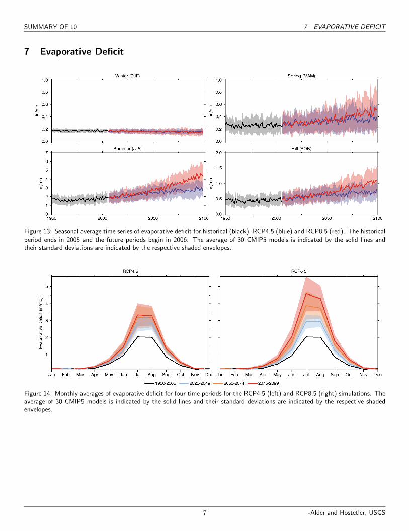
SUMMARY OF 10 7 EVAPORATIVE DEFICIT

7 Evaporative Deficit

Figure 13: Seasonal average time series of evaporative deficit for historical (black), RCP4.5 (blue) and RCP8.5 (red). The historicalperiod ends in 2005 and the future periods begin in 2006. The average of 30 CMIP5 models is indicated by the solid lines andtheir standard deviations are indicated by the respective shaded envelopes.

Figure 14: Monthly averages of evaporative deficit for four time periods for the RCP4.5 (left) and RCP8.5 (right) simulations. Theaverage of 30 CMIP5 models is indicated by the solid lines and their standard deviations are indicated by the respective shadedenvelopes.

7 -Alder and Hostetler, USGS

SUMMARY OF 10

8 Data

The temperature and precipitation summaries are created by spatially averaging the NASA NEX-DCP30 data set (Thrasher etal., 2013). The water-balance variables snow water equivalent, runoff, soil water storage and evaporative deficit are simulated byusing the NEX-DCP30 temperature and precipitation as input to a simple model (McCabe and Wolock, 2011). The water-balancemodel accounts for the partitioning of water through the various components of the hydrologic system, but does not account forgroundwater, diversions or regulation by impoundments.

9 Models

ACCESS1-0 bcc-csm1-1 bcc-csm1-1-m BNU-ESM CanESM2 CCSM4CESM1-BGC CMCC-CM CNRM-CM5 CSIRO-Mk3-6-0 FGOALS-g2 FIO-ESMGFDL-CM3 GFDL-ESM2G GFDL-ESM2M GISS-E2-R HadGEM2-AO HadGEM2-CCHadGEM2-ES inmcm4 IPSL-CM5A-LR IPSL-CM5A-MR IPSL-CM5B-LR MIROC5MIROC-ESM MIROC-ESM-CHEM MPI-ESM-LR MPI-ESM-MR MRI-CGCM3 NorESM1-M

10 Citation Information

Alder, J. R. and S. W. Hostetler, 2013. USGS National Climate Change Viewer. US Geological Surveyhttp://www.usgs.gov/climate_landuse/clu_rd/nccv.asp doi:10.5066/F7W9575T

McCabe, G. J., and D. M. Wolock, 2011. Independent effects of temperature and precipitation on modeled runoff in theconterminous United States, Water Resour. Res., 47, W11522, doi:10.1029/2011WR010630

Thrasher, B., J. Xiong, W. Wang, F. Melton, A. Michaelis, and R. Nemani, 2013. New downscaled climate projections suitablefor resource management in the U.S. Eos, Transactions American Geophysical Union 94, 321-323, doi:10.1002/2013EO370002

11 Disclaimer

These freely available, derived data sets were produced by J. Alder and S. Hostetler, US Geological Survey (USGS). The originalclimate data are from the NEX-DCP30 dataset, which was prepared by the Climate Analytics Group and NASA Ames ResearchCenter using the NASA Earth Exchange, and is distributed by the NASA Center for Climate Simulation. No warranty expressed orimplied is made by the USGS regarding the display or utility of the derived data on any other system, or for general or scientificpurposes, nor shall the act of distribution constitute any such warranty. The USGS shall not be held liable for improper or incorrectuse of the data described and/or contained herein.

8 -Alder and Hostetler, USGS