dr. alexander walsch [email protected] part ii ... - tum · technical university munich (tum)...

Industrial Embedded Systems - Design for Harsh Environment -

Dr. Alexander Walsch

[email protected]

Part II

WS 2011/12

Technical University Munich (TUM)

Recap: Practical Example

� Two PCBs (Printed Circuit Board)

� What do you remember from last lecture?

Slide2A. Walsch, IN2244 WS 2012/13

Recap: Practical Example

� Two PCBs (Printed Circuit Board)

� What do you remember from last lecture?

� Nothing?

� A CPU?

� An OpAmp

� Some more that looks familiar?


Part II: Requirements Engineering

Requirements Analysis

Requirements Specification

A. Walsch, IN 2244 WS2012/13 4

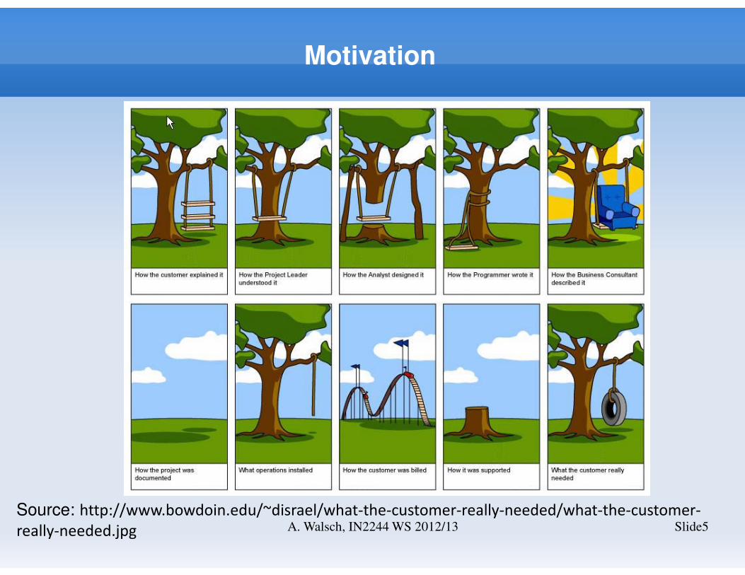
Motivation


Source: http://www.bowdoin.edu/~disrael/what-the-customer-really-needed/what-the-customer-

really-needed.jpg

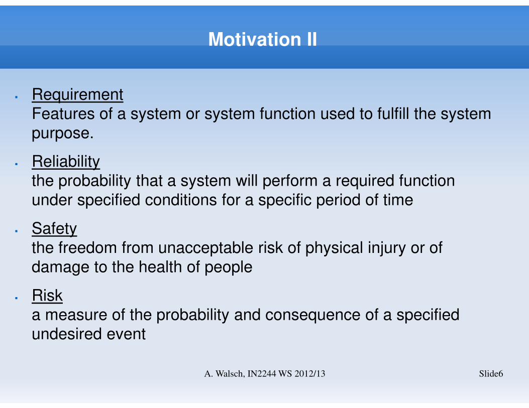
Motivation II


� Requirement

Features of a system or system function used to fulfill the system

purpose.

� Reliability

the probability that a system will perform a required function

under specified conditions for a specific period of time

� Safety

the freedom from unacceptable risk of physical injury or of

damage to the health of people

� Risk

a measure of the probability and consequence of a specified

undesired event

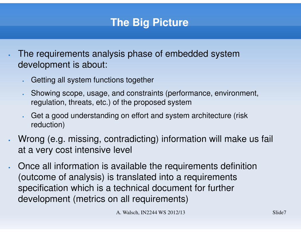
The Big Picture


� The requirements analysis phase of embedded system

development is about:

� Getting all system functions together

� Showing scope, usage, and constraints (performance, environment, regulation, threats, etc.) of the proposed system

� Get a good understanding on effort and system architecture (risk reduction)

� Wrong (e.g. missing, contradicting) information will make us fail

at a very cost intensive level

� Once all information is available the requirements definition

(outcome of analysis) is translated into a requirements

specification which is a technical document for further

development (metrics on all requirements)

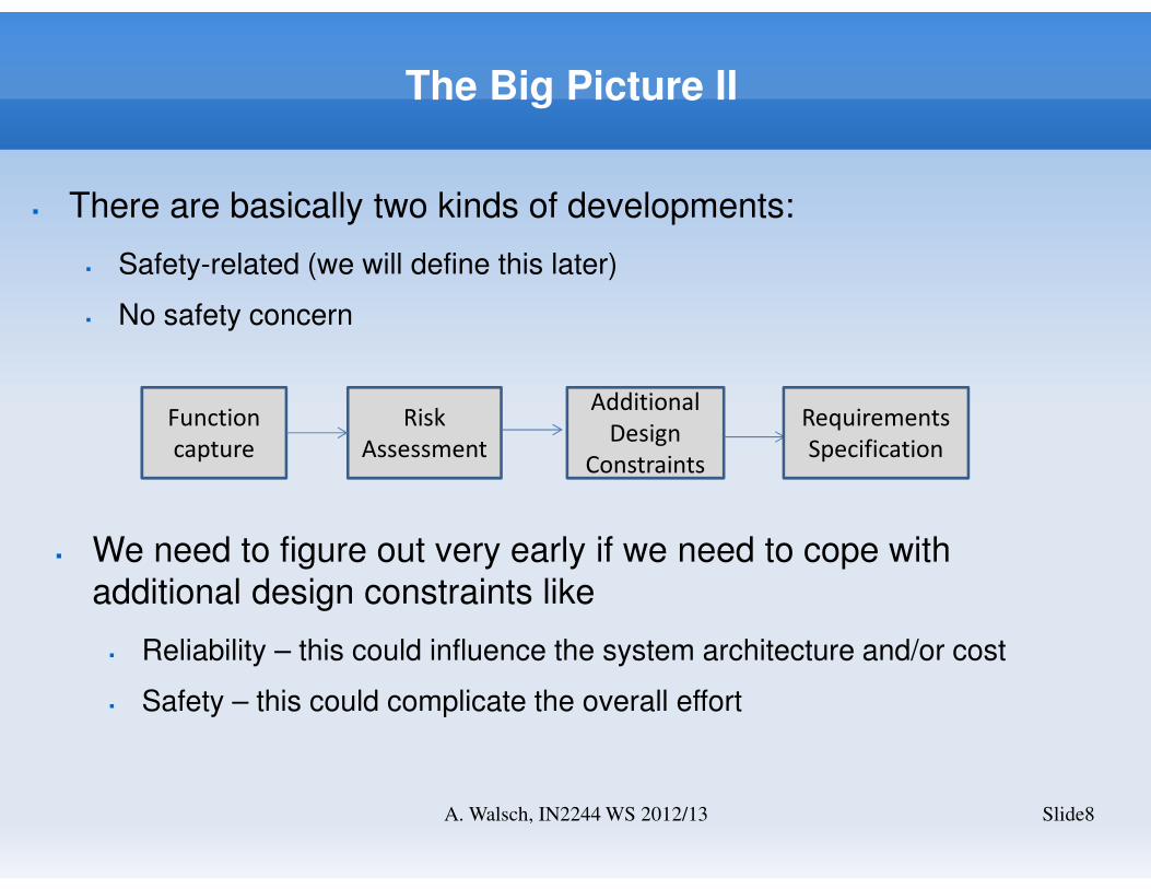
The Big Picture II


� There are basically two kinds of developments:

� Safety-related (we will define this later)

� No safety concern

� We need to figure out very early if we need to cope with

additional design constraints like

� Reliability – this could influence the system architecture and/or cost

� Safety – this could complicate the overall effort

Function

capture

Risk

Assessment

Additional

Design

Constraints

Requirements

Specification

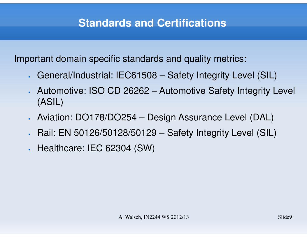
Standards and Certifications


Important domain specific standards and quality metrics:

� General/Industrial: IEC61508 – Safety Integrity Level (SIL)

� Automotive: ISO CD 26262 – Automotive Safety Integrity Level

(ASIL)

� Aviation: DO178/DO254 – Design Assurance Level (DAL)

� Rail: EN 50126/50128/50129 – Safety Integrity Level (SIL)

� Healthcare: IEC 62304 (SW)

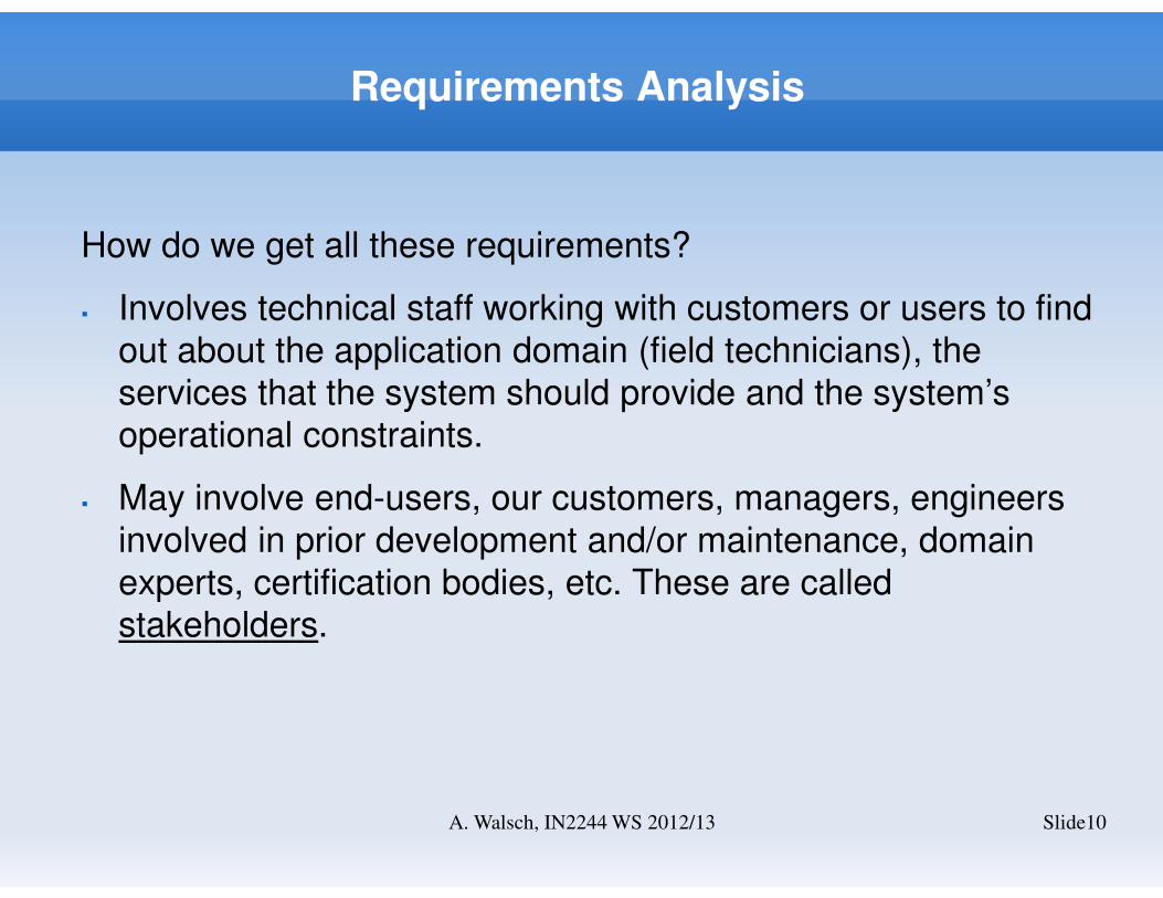
Requirements Analysis

How do we get all these requirements?

� Involves technical staff working with customers or users to find

out about the application domain (field technicians), the

services that the system should provide and the system’s

operational constraints.

� May involve end-users, our customers, managers, engineers

involved in prior development and/or maintenance, domain

experts, certification bodies, etc. These are called

stakeholders.


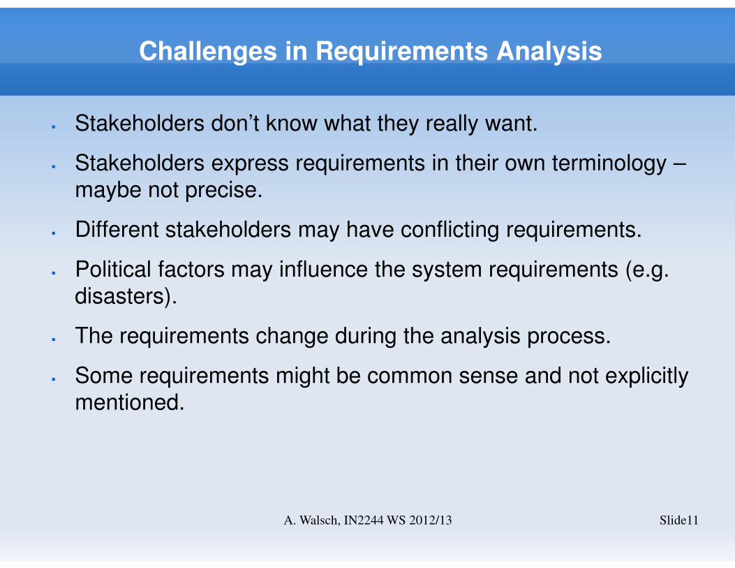
Challenges in Requirements Analysis

� Stakeholders don’t know what they really want.

� Stakeholders express requirements in their own terminology –

maybe not precise.

� Different stakeholders may have conflicting requirements.

� Political factors may influence the system requirements (e.g.

disasters).

� The requirements change during the analysis process.

� Some requirements might be common sense and not explicitly

mentioned.


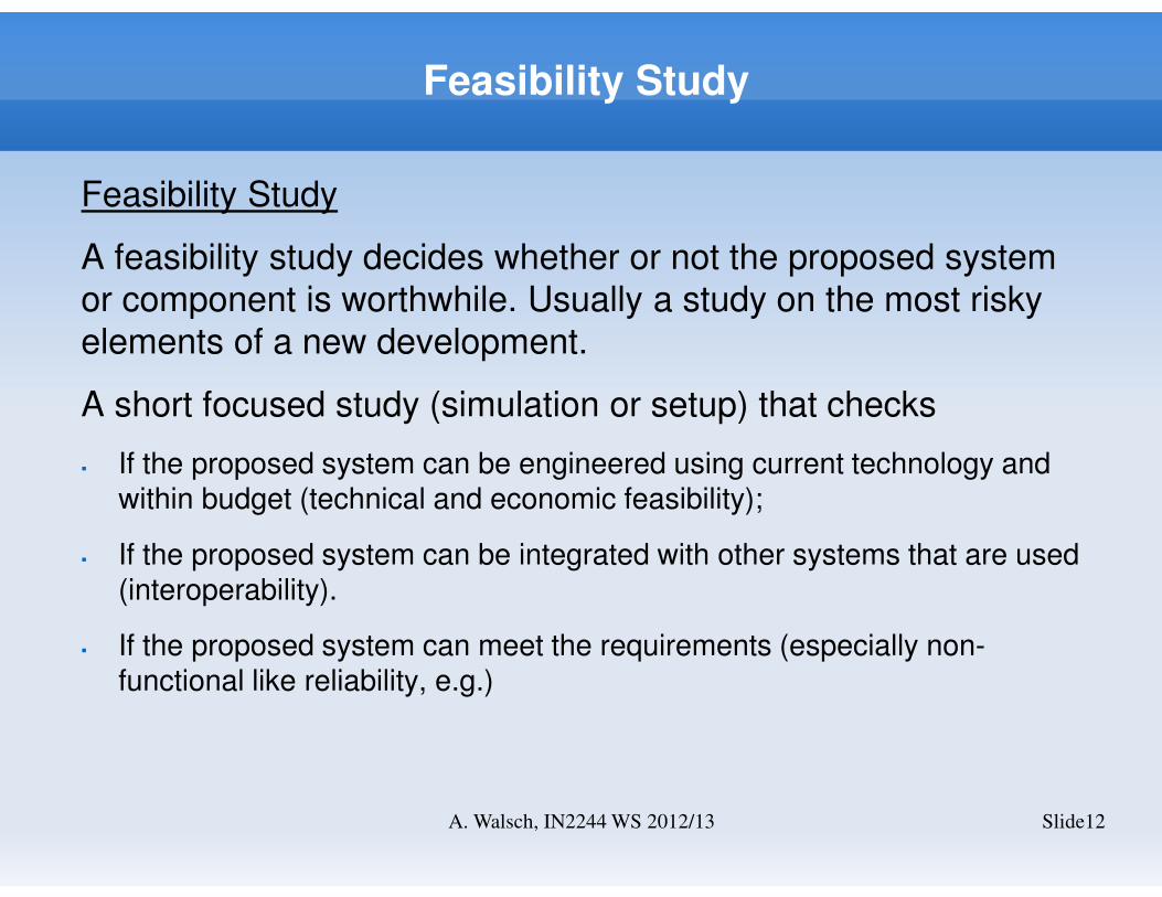
Feasibility Study

Feasibility Study

A feasibility study decides whether or not the proposed system

or component is worthwhile. Usually a study on the most risky

elements of a new development.

A short focused study (simulation or setup) that checks

� If the proposed system can be engineered using current technology and within budget (technical and economic feasibility);

� If the proposed system can be integrated with other systems that are used (interoperability).

� If the proposed system can meet the requirements (especially non-functional like reliability, e.g.)


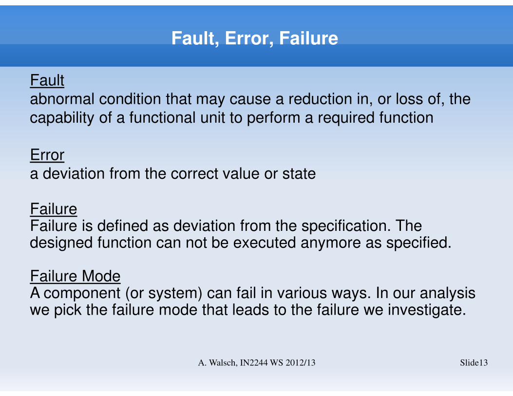
Fault, Error, Failure

Fault

abnormal condition that may cause a reduction in, or loss of, the

capability of a functional unit to perform a required function

Error

a deviation from the correct value or state

FailureFailure is defined as deviation from the specification. The designed function can not be executed anymore as specified.

Failure ModeA component (or system) can fail in various ways. In our analysis we pick the failure mode that leads to the failure we investigate.


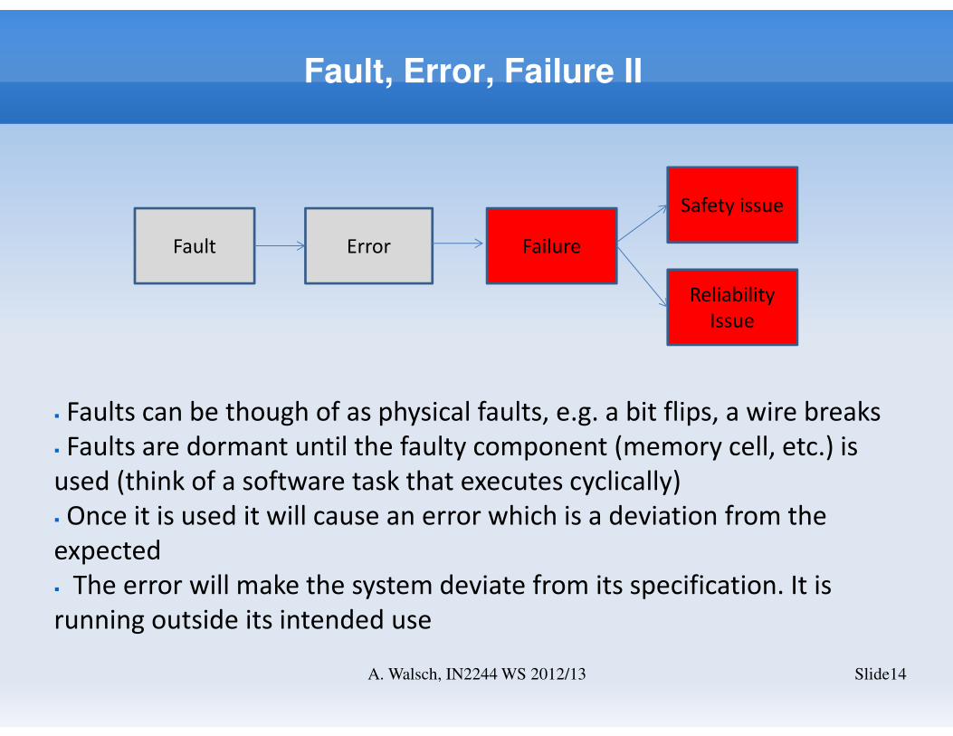
Fault, Error, Failure II


Fault Error Failure

Safety issue

Reliability

Issue

� Faults can be though of as physical faults, e.g. a bit flips, a wire breaks

� Faults are dormant until the faulty component (memory cell, etc.) is

used (think of a software task that executes cyclically)

� Once it is used it will cause an error which is a deviation from the

expected

� The error will make the system deviate from its specification. It is

running outside its intended use

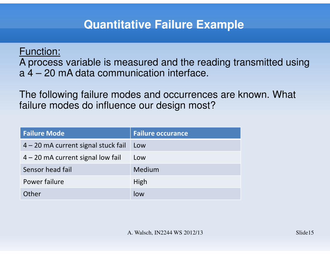
Quantitative Failure Example

Function:A process variable is measured and the reading transmitted using a 4 – 20 mA data communication interface.

The following failure modes and occurrences are known. What failure modes do influence our design most?


Failure Mode Failure occurance

4 – 20 mA current signal stuck fail Low

4 – 20 mA current signal low fail Low

Sensor head fail Medium

Power failure High

Other low

Failure Modes and Effect Analysis (FMEA)


� System FMEA in requirements analysis (proposed system)

� Also: Design FMEA (existing system)

� What are the failure modes and what is the effect:

� System failure (e.g. power, communication, timeliness, erroneous) mode assessment

� Plan how to prevent the failures

� How does it work?

� Identify potential failure modes and rate the severity (team activity)

� Evaluate objectively the probability of occurrence of causes and the ability to detect the cause when it occurs

� Rank failure modes and isolate the most critical ones

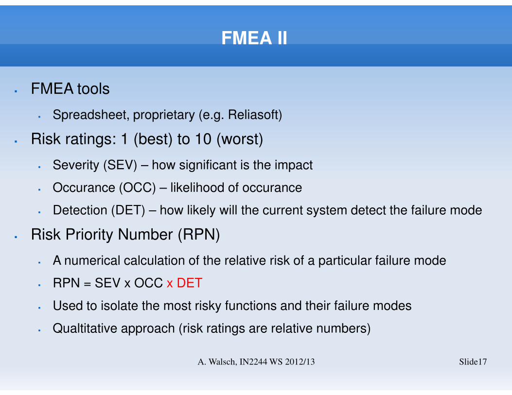
FMEA II


� FMEA tools

� Spreadsheet, proprietary (e.g. Reliasoft)

� Risk ratings: 1 (best) to 10 (worst)

� Severity (SEV) – how significant is the impact

� Occurance (OCC) – likelihood of occurance

� Detection (DET) – how likely will the current system detect the failure mode

� Risk Priority Number (RPN)

� A numerical calculation of the relative risk of a particular failure mode

� RPN = SEV x OCC x DET

� Used to isolate the most risky functions and their failure modes

� Qualtitative approach (risk ratings are relative numbers)

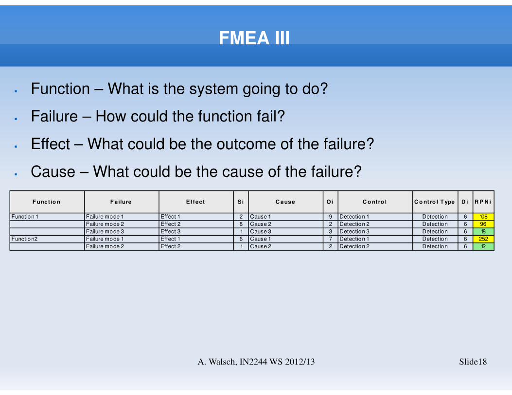
FMEA III


� Function – What is the system going to do?

� Failure – How could the function fail?

� Effect – What could be the outcome of the failure?

� Cause – What could be the cause of the failure?

F unct io n F ailure Effect Si C ause Oi C o ntro l C o ntro l T ype D i R P N i

Function 1 Failure mode 1 Effect 1 2 Cause 1 9 Detection 1 Detection 6 108

Failure mode 2 Effect 2 8 Cause 2 2 Detection 2 Detection 6 96


Function2 Failure mode 1 Effect 1 6 Cause 1 7 Detection 1 Detection 6 252


Fault Tree Analysis (FTA)


� Top event is failure mode

� Devide system into components

� Look into combinations of faults (strength of FTA)

� Tree like structure using combinatorical logic

� Paths of Failure

Outcome:

� Root cause event (external, internal) that (in combination) will lead

to top event

� Good system understanding – very useful if applied to existing

systems to isolate reliability issues

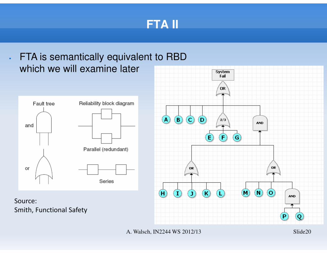
FTA II


Source:

Smith, Functional Safety

� FTA is semantically equivalent to RBD

which we will examine later

Where are we?

A. Walsch, IN 2244 WS2012/13 21

� We know that there are critical requirements that influence our

proposed system:

� What can we do about that?Are there any architecturural or technology decisions we should make early on?

� What metrics do we have?At this point we have only used categories but no real numbers. We need some metrics.

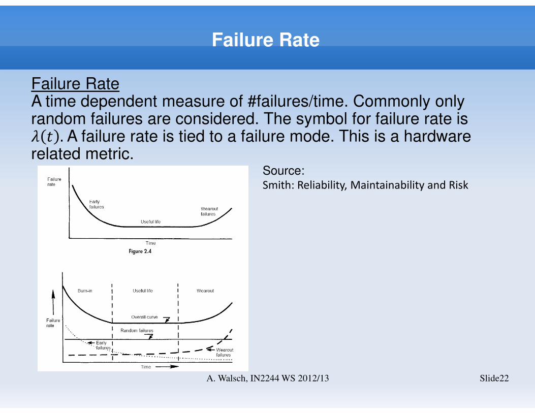
Failure Rate

Failure RateA time dependent measure of #failures/time. Commonly only random failures are considered. The symbol for failure rate is � � . A failure rate is tied to a failure mode. This is a hardware related metric.


Source: Smith: Reliability, Maintainability and Risk

Reliability

Reliability

Reliability of a system or component is defined to be the

probability that a given system or component will perform a

required function under specified conditions for a specified period

of time.

� “probability of non-failure (survival) in a given period”

� Reliability of a system function is modeled as:

R(t) = �� if the failure rate � is constant.

� λ is often expressed as failures per 106 hours or FIT (failures

per 109 hours).

� If “λt” small then R(t) = 1 - λt


Mean Time Between Failure (MTBF)

MTBF

Mean Time Between Failures (MTBF) is the average time a

system will run between failures. The MTBF is usually expressed

in hours.

Θ = � � � ��

�= � ��

�dt = λ

��, λ = const.

The observed MTBF (not all items have failed but k):

Θ� = T/k; T = total time, k = failed items (total N)


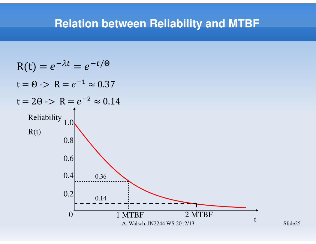
Relation between Reliability and MTBF

R(t) = �� = � /�

t = Θ -> R = �� ≈ 0.37

t = 2Θ -> R = � ≈ 0.14

t

Reliability

R(t)

1.0

0

0.8

0.6

0.4

0.2

1 MTBF 2 MTBF

0.36


0.14

Failure Rate Example

A system (S) has 10 components (C) with a failure rate of 5 per

106 hours each. Calculate λS and MTBF S. Consider two cases:

- All components are required to perform the function (single point

of failure)

- Each component performs a different function


Failure Rate Example II

A system (S) has 10 components (C) with a failure rate of 5 per

106 hours each. Calculate λS and MTBF S. Consider two cases:

A) All components are required to perform the function (single

point of failure)

B) Each component performs a different function

Solution A)

λC = 5 * 10-6 failures/hour

λS = 10 * 5 * 10-6 failures/hour = 5 * 10-5 failures/hour

ΘS = �

�#

= 20000h

Solution B)

λC = λS = 5 * 10-6 failures/hour; ΘS = �

�#

= 200000h


Mean Down Time (MDT)

MDT

Mean Down Time (MDT) is the average time a system is in a

failed state and can not execute its function.

MTBF can be understood as the mean up time.

MTTR

Mean Time to Repair (MTTR) is overlapping with MDT. Used for

maintenance calculations. It can be visualized as the average time

it takes (a technician) to repair the system such that it is up again.

We will not use MTTR in this lecture anymore.


Availability


Availability

Availability is the probability that a system is functioning at any

time during its scheduled working period.

$ = %& '()

* +, '()=

%& '()

%& '()-.*/0 '()=

1234

1234-152

similar:

calculation of unavailability (PFD)

Unavailability Example


λ = 10-6 failures/hour ; MDT = 10h

Unavailability = ?

Unavailability Example


λ = 10-6 failures/hour ; MDT = 10h

Unavailability = ?

$̅ = .*/0 '()

* +, '()=

152

1234-152≈ � ∗ 89:

-> $̅ = 10-5

We will need this metric when we look into safety later. This is an

important metric if a failure is dormant meaning the function is not

performed immediately.

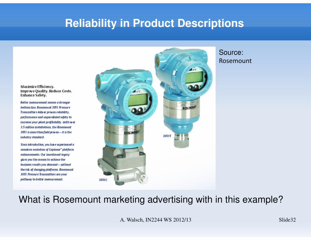
Reliability in Product Descriptions


Source: Rosemount

What is Rosemount marketing advertising with in this example?

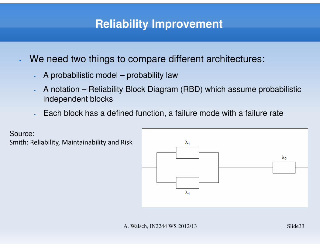
Reliability Improvement

� We need two things to compare different architectures:

� A probabilistic model – probability law

� A notation – Reliability Block Diagram (RBD) which assume probabilistic independent blocks

� Each block has a defined function, a failure mode with a failure rate


Source: Smith: Reliability, Maintainability and Risk

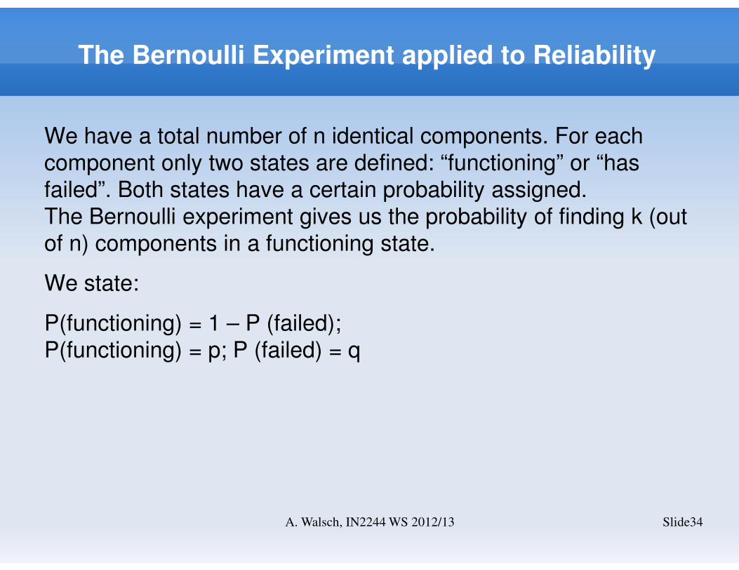
The Bernoulli Experiment applied to Reliability

We have a total number of n identical components. For each

component only two states are defined: “functioning” or “has

failed”. Both states have a certain probability assigned.

The Bernoulli experiment gives us the probability of finding k (out

of n) components in a functioning state.

We state:

P(functioning) = 1 – P (failed);

P(functioning) = p; P (failed) = q


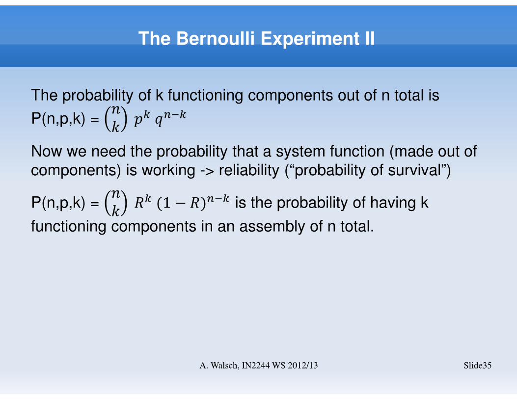
The Bernoulli Experiment II

The probability of k functioning components out of n total is

P(n,p,k) = ;< =>?0�>

Now we need the probability that a system function (made out of

components) is working -> reliability (“probability of survival”)

P(n,p,k) = ;< �>(1 − �)0�> is the probability of having k

functioning components in an assembly of n total.


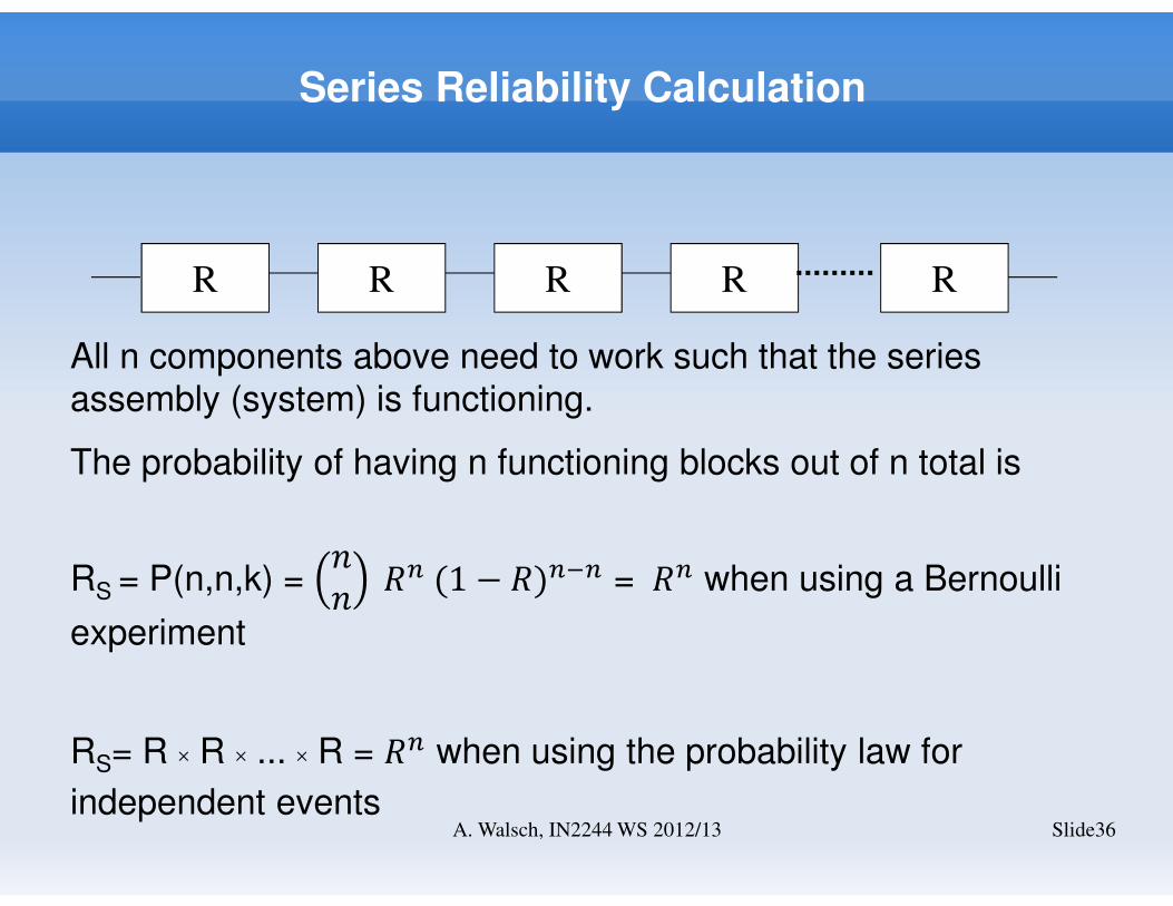
Series Reliability Calculation


R R R R R

All n components above need to work such that the series

assembly (system) is functioning.

The probability of having n functioning blocks out of n total is

RS = P(n,n,k) = ;; �0(1 − �)0�0 = �0 when using a Bernoulli

experiment

RS= R × R × ... × R = �0 when using the probability law for

independent events

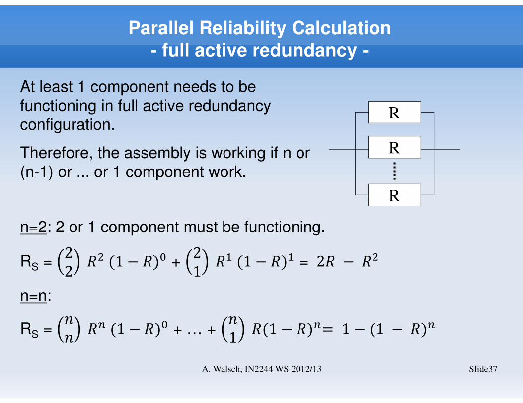
Parallel Reliability Calculation- full active redundancy -


At least 1 component needs to be

functioning in full active redundancy

configuration.

Therefore, the assembly is working if n or

(n-1) or ... or 1 component work.

R

R

R

n=2: 2 or 1 component must be functioning.

RS = 22 � (1 − �)� +

21 ��(1 − �)� = 2� − �

n=n:

RS = ;; �0(1 − �)� + … +

;1 �(1 − �)0= 1 − (1 − �)0

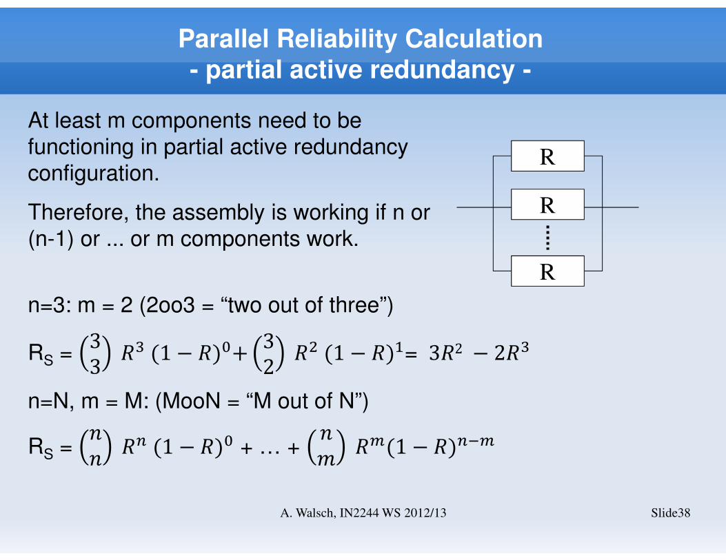
Parallel Reliability Calculation- partial active redundancy -


At least m components need to be

functioning in partial active redundancy

configuration.

Therefore, the assembly is working if n or

(n-1) or ... or m components work.

R

R

R

n=3: m = 2 (2oo3 = “two out of three”)

RS = 33 �A(1 − �)�+ 3

2 � (1 − �)�= 3�2 − 2�An=N, m = M: (MooN = “M out of N”)

RS = ;; �0(1 − �)� + … +

;C �((1 − �)0�(

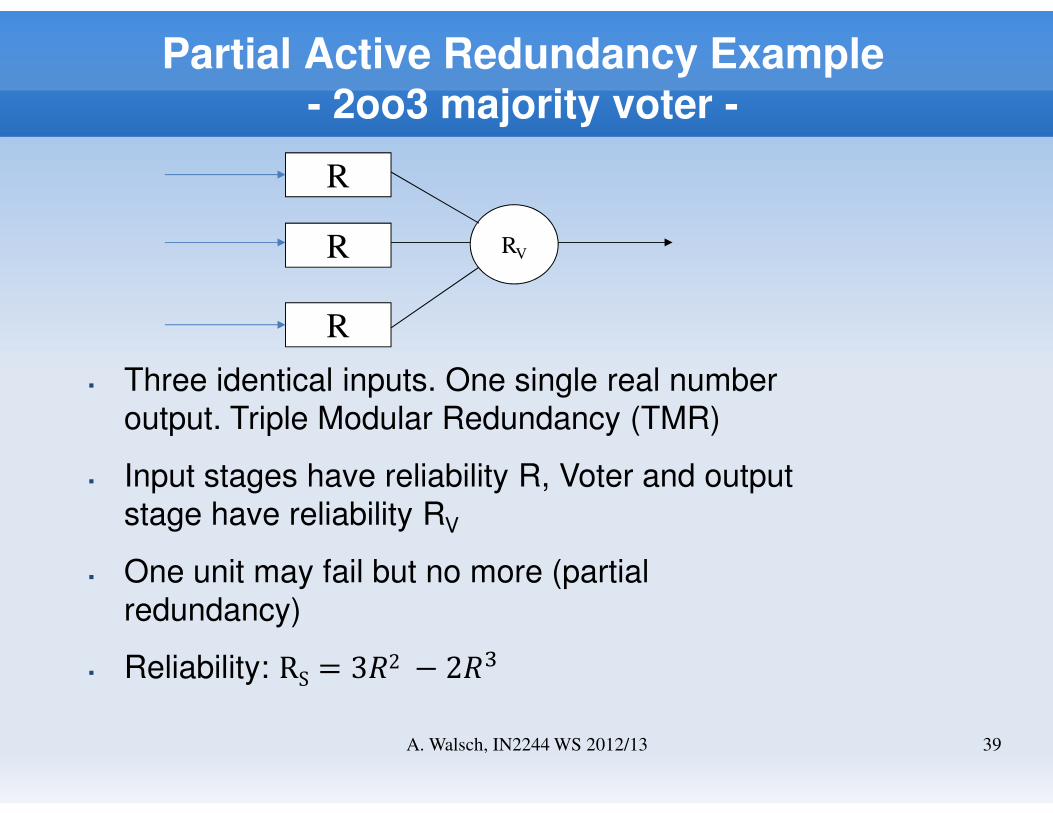
Partial Active Redundancy Example- 2oo3 majority voter -

R

R

R

RV

� Three identical inputs. One single real number

output. Triple Modular Redundancy (TMR)

� Input stages have reliability R, Voter and output

stage have reliability RV

� One unit may fail but no more (partial

redundancy)

� Reliability: RS = 3�2 − 2�A39A. Walsch, IN2244 WS 2012/13

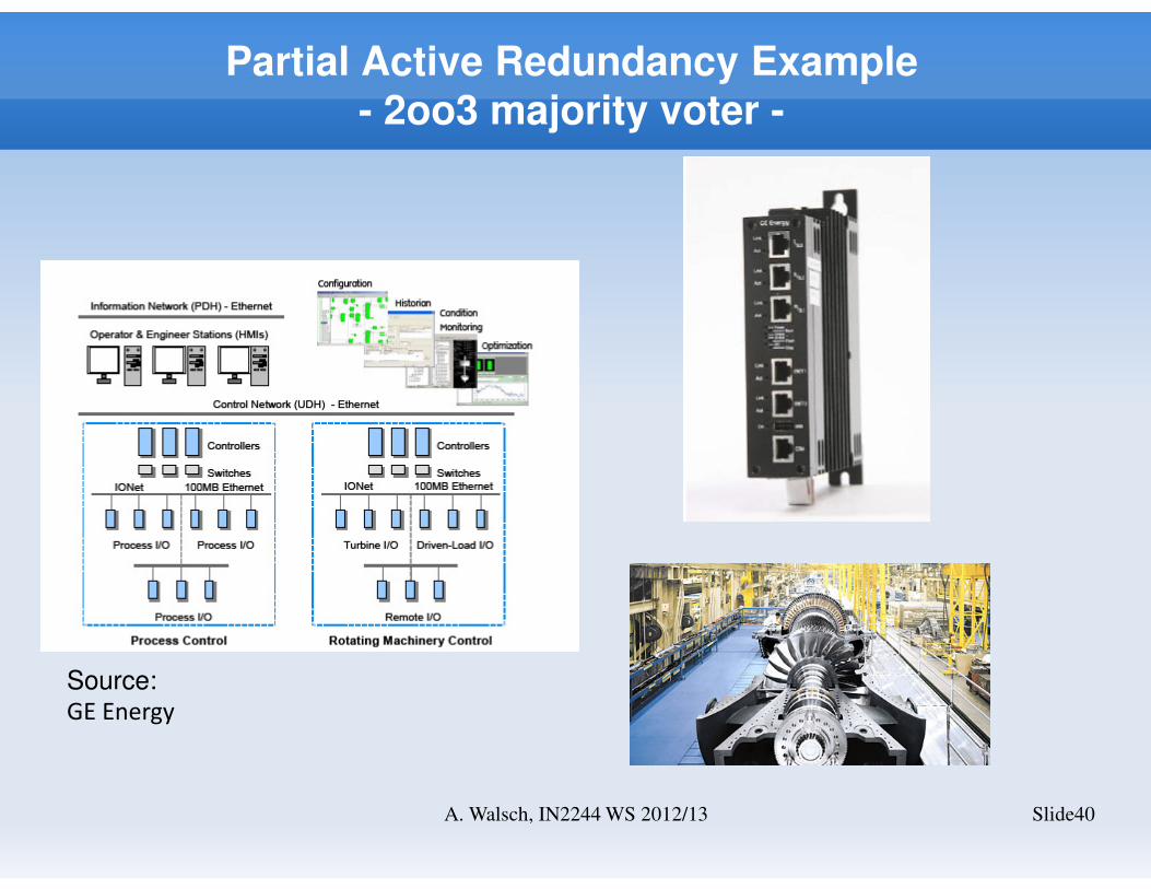
Partial Active Redundancy Example- 2oo3 majority voter -


Source: GE Energy

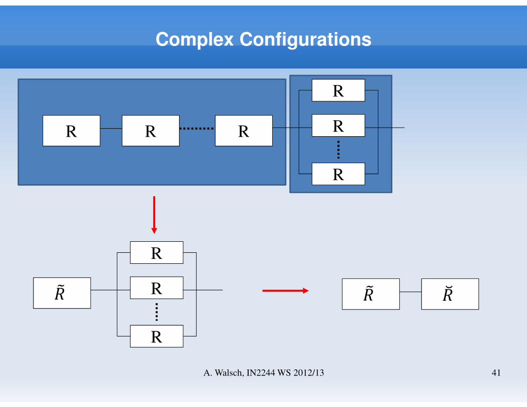
Complex Configurations

R R R

R

R

R

41A. Walsch, IN2244 WS 2012/13

�ER

R

R

�E �F

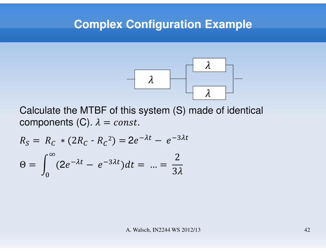
Complex Configuration Example

��

42A. Walsch, IN2244 WS 2012/13

Calculate the MTBF of this system (S) made of identical

components (C). � = GH;I�.�# =�J ∗ (2�J - �J2) =2�� −�A�

Θ =K (2�� −�A� �

�)�� = … = 23�

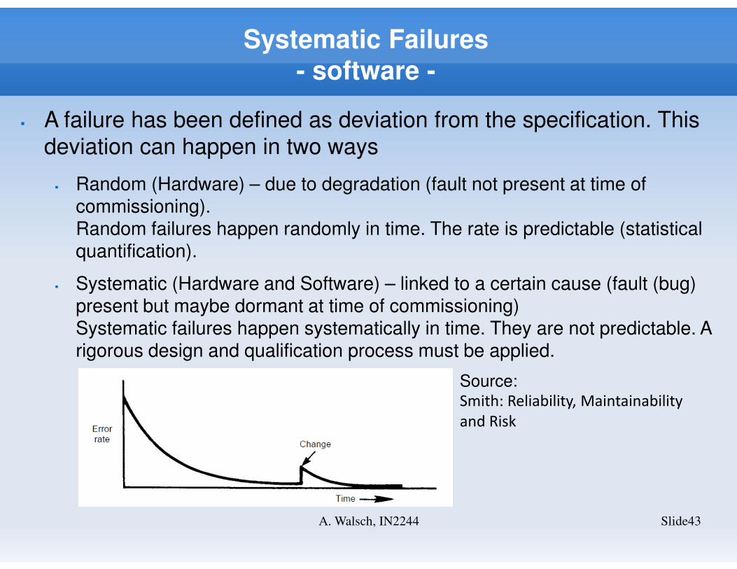
Systematic Failures- software -

Slide43A. Walsch, IN2244

� A failure has been defined as deviation from the specification. This

deviation can happen in two ways

� Random (Hardware) – due to degradation (fault not present at time of commissioning).Random failures happen randomly in time. The rate is predictable (statistical quantification).

� Systematic (Hardware and Software) – linked to a certain cause (fault (bug) present but maybe dormant at time of commissioning)Systematic failures happen systematically in time. They are not predictable. A rigorous design and qualification process must be applied.

Source: Smith: Reliability, Maintainability

and Risk

Questions?


dr. alexander walsch [email protected] part ii ... - tum · technical university munich (tum)...

Documents