1

Distribution Systems Hardening against NaturalDisasters

Yushi Tan, Student Member, IEEE Arindam K. Das, Member, IEEE, Payman Arabshahi, Senior Member, IEEE,and Daniel S. Kirschen, Fellow, IEEE

Abstract—Distribution systems are often crippled by catas-trophic damage caused by a natural disaster. Well-designedhardening can significantly improve the performance of post-disaster restoration operations. Such performance is quantifiedby a resilience measure associated with the operability trajectory.The distribution system hardening problem can be formulatedas a two-stage stochastic problem, where the inner operationalproblem addresses the proper scheduling of post-disaster repairsand the outer problem the judicious selection of components toharden. We propose a deterministic single crew approximationwith two solution methods, an MILP formulation and a heuristicapproach. We provide computational evidence on various IEEEtest feeders which illustrates that the heuristic approach providesnear-optimal hardening solutions efficiently.

I. INTRODUCTION

NATURAL disasters have caused major damage to elec-tricity distribution networks and deprived homes and

businesses of electricity for prolonged periods, for exampleHurricane Sandy in November 2012 [1], the ChristchurchEarthquake in February 2011 [2] and the June 2012 Mid-Atlantic and Midwest Derecho [3]. Estimates of the annualcost of power outages caused by severe weather between 2003and 2012 range from $18 billion to $33 billion on average[4]. Physical damage to grid components must be repairedbefore power can be restored [1], [5]. On the operational side,approaches have been proposed for scheduling the availablerepair crews in order to minimize the cumulative duration ofcustomer interruption, which reduces the harm done to theaffected community [6]–[8]. On the planning side, Kwasinskiet al. [2] reported facilities that had been upgraded or hardenedin Christchurch, at a cost of $5 million, remained service-able immediately after the September 2010 earthquake andsaved approximately $30 to $50 million in subsequent repairs.Hardening minimizes the potential damages caused by dis-ruptions, thereby facilitating restoration and recovery efforts,and the time it takes for the infrastructure system to resumeoperation [9]. However, as indicated in [10], the difficultyof hardening does not lie in the design or construction of ahardened system, rather in the ability to quantify the expectedperformance improvement so that rational decisions can bemade regarding increased cost versus potential future benefit.

This material is based upon work supported by the National ScienceFoundation under Grant No.1509880: Quantifying the Resilience of PowerSystems to Natural Disasters.

Y. Tan, P. Arabshahi and D. S. Kirschen are with the Department ofElectrical Engineering, University of Washington, Seattle, WA, 98195-2500USA. (Email: ystan@uw.edu)

A. K. Das is with the Department of Electrical Engineering, EasternWashington University, Cheney, WA, 99004-2493, USA.

A. Concept and quantification of resilienceResilience in infrastructure systems under natural disas-

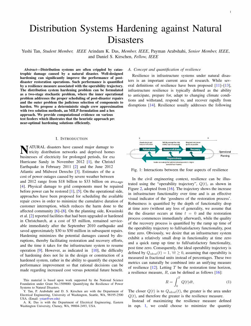
ters is an important current area of research. While sev-eral definitions of resilience have been proposed [11]–[13],infrastructure resilience is typically defined as the abilityto anticipate, prepare for, adapt to changing climate condi-tions and withstand, respond to, and recover rapidly fromdisruptions [14]. Resilience usually addresses the followingfour aspects - preparedness, robustness, resourcefulness andrecovery, as illustrated in Fig. 1, which is adapted from the‘Resilience Construct’ in [15]. Since resourcefulness mainlydepends on people instead of technology, the planning aspect,preparedness, should be guided by the other two operationalaspects, robustness and recovery.

Robustness Resourcefulness

Fig. 1: Interactions between the four aspects of resilience

In the civil engineering context, resilience can be illus-trated using the “operability trajectory”, Q(t), as shown inFigure 2, adopted from [16]. The trajectory shows the increasein infrastructure functionality over time and is an effectivevisual indicator of the ‘goodness of the restoration process’.Robustness is quantified by the depth of functionality dropat time zero (without any loss of generality, we assume thatthe the disaster occurs at time t = 0 and the restorationprocess commences immediately afterward), while the qualityof the recovery process is quantified by the ramp up time ofthe operability trajectory to full/satisfactory functionality, posttime zero. Obviously, we desire that an infrastructure systemexhibit a relatively small drop in functionality at time zeroand a quick ramp up time to full/satisfactory functionality,post time zero. Consequently, the ideal operability trajectory isdefined by Qideal(t) = 1, ∀t ≥ 0, assuming that operability ismeasured in fractional units instead of percentages. These twometrics can naturally be combined into an unifying measureof resilience [12]. Letting T be the restoration time horizon,a resilience measure, R, can be defined as follows [16]:

R =

∫ T

0

Q(t)dt, (1)

The closer Q(t) is to Qideal(t), the greater is the area underQ(t), and therefore the greater is the resilience measure.

Instead of maximizing the resilience measure definedin eqn. 1, we could choose to minimize the quantity

2

∫ T0Qideal(t)dt−

∫ T0Q(t)dt, which is the area over the Q(t)

curve, bounded from above by Qideal(t). This area, informally,the ‘other side of resilience’, can be interpreted as a measureof ‘aggregate harm’. In a power system, it can be shown usingthe Lebesgue integral that minimizing this area is equivalentto minimizing the quantity

∑n wnTn, where wn can be

interpreted as the contribution of node n to the overall loss infunctionality of the system or the importance of node n andTn is the time to restore node n. Therefore, the objective foroperational problems is to minimize the measure

∑n wnTn,

given a specific disaster scenario, while the objective forplanning problems is to minimize

∑n wnTn in an expected

sense, where the expectation is over all possible disasterscenarios.

0

20

40

60

80

100

120

-10 0 10 20 30 40 50 60

Funct

ional

ity

in P

erc

enta

ge

Day relative to the second Hurricane Katrina Landfall; day 0 = landfall

Operability trajectory from Hurricane Katrina

Robust

ness

Recovery

Fig. 2: Operability trajectory after Hurricane Katrina [16].

B. Literature review

Defending critical infrastructures at the transmission levelhas been a major research focus over the past decade [17]–[19]. In general, this research adopted the setting of Stack-elberg game and formulated the problem with a tri-leveldefender-attacker-defender model. Such a model assumes thatthe attacker has perfect knowledge of how the defender willoptimally operate the system after the attack and the attackermanipulates the system to its best advantage.

In recent years, several researchers have investigated dif-ferent methods for distribution systems hardening, but mostfocus solely on the robustness, i.e., worst-case load sheddingat the onset of disaster. Of note, a resilient distribution networkplanning problem (RDNP) was proposed in [20] to coordinatethe hardening and distributed generation resource allocation. Atri-level defender-attacker-defender model is studied, in whichthe defender (hardening planner) selects a network hardeningplan in the first stage, the attacker (natural disaster) disrupts thesystem with an interdiction budget, and finally, the defender(the distribution system operator) reacts by controlling DGsand switches in order to minimize the shed load. This modelis improved in [21] by considering the investment cost and byeliminating the assumption that enhanced components shouldremain intact during any disaster scenario. Another directionof research enforces chance constraints on the loss of criticalloads and normal loads respectively [22], [23]. A two-stagestochastic program and heuristic solution of hardening strategy

were proposed in [24], specifically for earthquake hazards,under the assumption that the repair times for similar types ofcomponents follow an uniform distribution, which simplifiesthe problem to a certain extent.

C. Our approach

To the best of our knowledge, this paper is the first toconsider the restoration process in conjunction with hardening.Our approach can be seen as a two-stage stochastic problem.The first stage selects from the set of potential hardeningchoices and determines the extent of hardening to maximizethe expected resilience measure R, while the second stagesolves the operational problem in each possible scenario by op-timizing the sequence of repairs given the hardening results. Inthe operational problem, we consider scheduling post-disasterrepairs in distribution network with parallel repair crews. Thisissue will be discussed in more detail in Section VI. Sincean ideal formulation of the problem is hard to solve andalso turns out impractical, we developed a deterministic singlecrew approximation with a heuristic approach to solve thehardening problem. Wang et al. [25] make a distinctionbetween hardening activities and resiliency activities whichare focused on the effectiveness of humans post-disaster. Byusing only one repair crew in the operational problem, we canalso focus on the effects of network structure and components,and reduce the reliance on resourcefulness (i.e. the number ofrepair crews available).

The rest of the paper is organized as follows. In Section II,we briefly review the operational problem of scheduling post-disaster repairs in distribution networks with multiple repaircrews and discuss an algorithm that converts an optimal singlecrew repair schedule to an arbitrary m-crew schedule witha proven performance bound. An MILP model for solvingthe single crew repair sequencing problem is also discussedin this section. In Section III, we formulate the problem ofdistribution system hardening against natural disasters andmodel it as a stochastic optimization problem, followed bya deterministic reformulation (Section IV) and single crewapproximation (Section V). In Section VI, we motivate whywe believe it is important to consider the restoration process(operational phase) in the hardening problem (planning phase)and develop the so called ‘restoration process aware hardeningproblem’. Two solution methods, an MILP formulation and aniterative heuristic algorithm, are also discussed in this section.The performance of these methods is validated by various casestudies on various standard IEEE test feeders in Section VII.

II. SCHEDULING POST-DISASTER REPAIRS INDISTRIBUTION NETWORKS

In this section, we briefly review the operational problem ofscheduling post-disaster repairs in distribution networks withmultiple repair crews. Further details can be found in [6].

A. Distribution networks modeling

A distribution network can be modeled by a graph G witha set of nodes N and a set of edges L. Let S ⊂ N represent

3

the set of source nodes which are initially energized andD = N \ S represent the set of sink nodes where consumersare located. An edge in G represents a distribution feederor some other connecting component. We assume that thenetwork topology G is radial, which is a valid assumption formany electricity distribution networks. Instead of a rigorouspower flow model, we model network connectivity using asimple network flow model, i.e., as long as a sink node isconnected to the source, we assume that all the loads connectdto this node can be supplied without violating any securityconstraint. For simplicity, we treat the three-phase distributionnetwork as if it were a single-phase system. Our analysis couldbe extended to a three-phase system using a multi-commodityflow model, as in [26].

B. Damage modeling

Let LD denote the set of damaged edges. Without loss ofgenerality, we assume that there is only one source node in G.If an edge is damaged, all downstream nodes lose power dueto lack of electrical connectivity. Each damaged edge l ∈ LDhas a (potentially) unique repair time pl. At the operationalstage, we assume perfect knowledge of the set LD and thecorresponding repair times, while, at the planning stage, therepair times are modeled as random variables following someprobability distribution.

C. Scheduling post-disaster repairs

Let wn be a nonnegative quantity that captures the im-portance of the load at node n. The importance of a nodecan depend on multiple factors, including but not limited to,the amount of load connected to it, the type of load served,and interdependency with other critical infrastructures. Forexample, re-energizing a node supplying a major hospitalshould receive a higher priority than a node supplying a similaramount of residential load. Similarly, it is likely that a nodethat provides electricity to a water sanitation plant would beassigned a higher priority. These priority factors would needto be assigned by the utility and their determination is outsidethe scope of this paper. In this paper We assume that the wn’sare known.

Based on conversations with an industry expert, we alsomake the assumption that crew travel times in a typicaldistribution network are small compared with the time requiredfor each repair. These travel times are therefore neglectedas a first order approximation. Additionally, since hardeningdecisions are made at the planning stage, it is unrealistic toexpect an accurate prediction what travel times might be whena disaster occurs. Within this framework, the operational goalis therefore to find a schedule by which the damaged linesshould be repaired such that the aggregate harm,

∑n∈N wnTn,

is minimized.We construct two simplified directed radial graphs to model

the effect that the topology of the distribution network hason scheduling. The first graph, G′, is called the ‘damagedcomponent graph’. All nodes in G that are connected by intactedges are contracted into a supernode in G′. The set of edgesin G′ is the set of damaged lines in G, LD. The directions

to these edges follow trivially from the network topology. Thesecond graph, P , is called a ‘soft precedence constraint graph’,and is constructed as follows. The nodes in this graph are thedamaged lines in G and an edge exists between two nodes inthis graph if they share the same node in G′. Such a graphenables us to consider the hierarchal relationships betweendamaged lines, which we define as soft precedence constraints.See Fig. 4 for examples of P and G′.

Fig. 3: IEEE 13 Node Test Feeder

(a) G′ graph (b) P graph

Fig. 4: (a) The damaged component graph, G′, obtained fromFig. 3, assuming that the damaged edges are 650−632, 632−645, 684 − 611 and 671 − 692. (b) The corresponding softprecedence graph, P .

Two different time vectors are of interest in the operationalproblem: a vector of completion times of line repairs, denotedby Cl’s, and a vector of energization times of nodes, denotedby En’s. While we have so far associated the term ‘energiza-tion time’ with nodes in a given network topology, G, it isalso possible to define energization times for the lines. Givena directed edge l ∈ G′, let h(l) and t(l) denote its head and tailnodes, i.e., l = h(l)→ t(l). Then, El = Et(l), where El is theenergization time of line l and Et(l) is the energization timeof the node t(l) in G. Analogously, the weight of node t(l),wt(l), can be interpreted as a weight on the line l, wl. The softprecedence constraints, i ≺S j, therefore implies that line jcannot be energized unless line i is energized, or equivalently,Ej ≥ Ei.

4

D. Solution methods for optimal single crew repair sequenc-ing

We begin with the following lemma, which connects theproblem defined above to a well studied problem in schedul-ing theory, for which a polynomial time optimal algorithmexists [27]. A proof of this lemma can be found in [6].

Lemma 1. Single crew repair and restoration scheduling indistribution networks is equivalent to 1 | outtree |

∑wjCj ,

where the outtree precedences are given in the soft precedenceconstraint graph P .

The problem of 1 | outtree |∑wjCj can be solved in

polynomial time. Algorithm 1 shown below is based on thealgorithm in Chapter 4 of [28], which solves this problem inO(n logn) time (see Theorem 4.8 in [28]). Additional detailsand an example can be found in [6].

Algorithm 1 Optimal algorithm for single crew restoration indistribution networks. The input to this algorithm is the prece-dence graph P . The notation pred(n) denotes the predecessorof any node n ∈ P .

1: w(1)← −∞; pred(1)← 0;2: for n = 1 to |N(P )| do3: A(n)← n; Bn ← n; q(n)← w(n)/p(n);4: end for5: for n = 2 to |N(P )| do6: pred(n)← parent of n in P ;7: end for8: nodeSet← 1, 2, · · · , |N(P )|;9: while nodeSet 6= 1 do

10: Find j ∈ nodeSet such that q(j) is largest;% ties can be broken arbitrarily

11: Find i such that pred(j) ∈ Bi, i = 1, 2, . . . |N(P )|;12: w(i)← w(i) + w(j);13: p(i)← p(i) + p(j);14: q(i)← w(i)/p(i);15: pred(j)← A(i);16: A(i)← A(j);17: Bi ← Bi, Bj; % ‘,’ denotes concatenation18: nodeSet← nodeSet \ j;19: end while

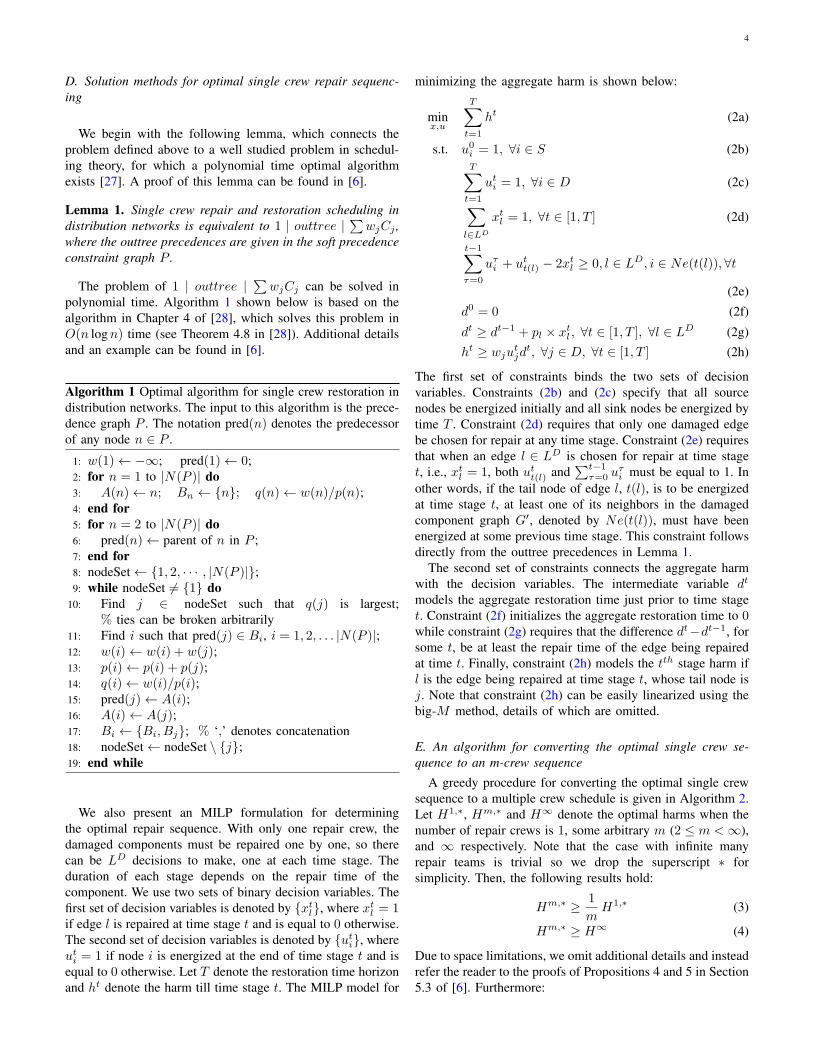
We also present an MILP formulation for determiningthe optimal repair sequence. With only one repair crew, thedamaged components must be repaired one by one, so therecan be LD decisions to make, one at each time stage. Theduration of each stage depends on the repair time of thecomponent. We use two sets of binary decision variables. Thefirst set of decision variables is denoted by xtl, where xtl = 1if edge l is repaired at time stage t and is equal to 0 otherwise.The second set of decision variables is denoted by uti, whereuti = 1 if node i is energized at the end of time stage t and isequal to 0 otherwise. Let T denote the restoration time horizonand ht denote the harm till time stage t. The MILP model for

minimizing the aggregate harm is shown below:

minx,u

T∑t=1

ht (2a)

s.t. u0i = 1, ∀i ∈ S (2b)T∑t=1

uti = 1, ∀i ∈ D (2c)∑l∈LD

xtl = 1, ∀t ∈ [1, T ] (2d)

t−1∑τ=0

uτi + utt(l) − 2xtl ≥ 0, l ∈ LD, i ∈ Ne(t(l)),∀t

(2e)

d0 = 0 (2f)

dt ≥ dt−1 + pl × xtl , ∀t ∈ [1, T ], ∀l ∈ LD (2g)ht ≥ wjutjdt, ∀j ∈ D, ∀t ∈ [1, T ] (2h)

The first set of constraints binds the two sets of decisionvariables. Constraints (2b) and (2c) specify that all sourcenodes be energized initially and all sink nodes be energized bytime T . Constraint (2d) requires that only one damaged edgebe chosen for repair at any time stage. Constraint (2e) requiresthat when an edge l ∈ LD is chosen for repair at time staget, i.e., xtl = 1, both utt(l) and

∑t−1τ=0 u

τi must be equal to 1. In

other words, if the tail node of edge l, t(l), is to be energizedat time stage t, at least one of its neighbors in the damagedcomponent graph G′, denoted by Ne(t(l)), must have beenenergized at some previous time stage. This constraint followsdirectly from the outtree precedences in Lemma 1.

The second set of constraints connects the aggregate harmwith the decision variables. The intermediate variable dt

models the aggregate restoration time just prior to time staget. Constraint (2f) initializes the aggregate restoration time to 0while constraint (2g) requires that the difference dt−dt−1, forsome t, be at least the repair time of the edge being repairedat time t. Finally, constraint (2h) models the tth stage harm ifl is the edge being repaired at time stage t, whose tail node isj. Note that constraint (2h) can be easily linearized using thebig-M method, details of which are omitted.

E. An algorithm for converting the optimal single crew se-quence to an m-crew sequence

A greedy procedure for converting the optimal single crewsequence to a multiple crew schedule is given in Algorithm 2.Let H1,∗, Hm,∗ and H∞ denote the optimal harms when thenumber of repair crews is 1, some arbitrary m (2 ≤ m <∞),and ∞ respectively. Note that the case with infinite manyrepair teams is trivial so we drop the superscript ∗ forsimplicity. Then, the following results hold:

Hm,∗ ≥ 1

mH1,∗ (3)

Hm,∗ ≥ H∞ (4)

Due to space limitations, we omit additional details and insteadrefer the reader to the proofs of Propositions 4 and 5 in Section5.3 of [6]. Furthermore:

5

Algorithm 2 Algorithm for converting the optimal single crewschedule to an m-crew schedule

Treat the optimal single crew repair sequence as a prioritylist, and, whenever a crew is free, assign to it the next jobfrom the list. The first m jobs in the single crew repairsequence are assigned arbitrarily to the m crews.

Proposition 1. Let Hm be the harm corresponding to an m-crew schedule, obtained by application of Algorithm 2 on anoptimal single crew sequence (which can be computed usingAlgorithm 1). Then:

Hm ≤ 1

mH1,∗ +

m− 1

mH∞ (5)

Proof. See proof of Theorem 4 in Section 5.3 of [6].

Consequently,

Theorem 1. Algorithm 2 is a(2− 1

m

)approximation. That

is:Hm ≤

(2− 1

m

)Hm,∗

Proof. Follows straightforwardly from eqns (3) ∼ (5).

III. THE HARDENING PROBLEM: FORMULATION

A. Damage modeling

As mentioned above, damages are modeled by repair timevectors associated with network components. Since no apriori exact information about the damages is available atthe planning stage, we model the repair times as a randomvector ~P . The uncertainties are twofold: all possible naturaldisasters that planners want to take into account and theuncertain damages to components caused by a specific dis-aster. The distribution of ~P can be a mixture of a Bernoullidistribution which represents the probability of damage anda (possibly) continuous distribution of repair time, such asthe exponential [29] or log-normal distribution [30]. Mixeddistributions, usually do not admit a closed-form expression oftheir distribution functions. In our work, we do not assume anyknowledge of the distribution function, except for knowledgeof the first moment E[~P].

Some planners tend to use the sample average approxima-tion (SAA) methods by considering a limited set of componentdamage scenarios, which are either defined by users or drawnfrom a probabilistic model, as in [22], [23]. It is known thatSAA methods converge to the optimal solution as the samplesize goes to infinity. However, SAA methods require that theselected scenarios be typical and right on target, or the sampleaveraging needs to be performed over a large number of cases.

B. Hardening options and costs

In practice, multiple hardening actions are usually availablefor each network component. For example, hardening an edgecan involve some combination of vegetation management,pole reinforcement, undergrounding, enhanced pole guying,

[21]. Typically, the goal of hardening a component is tolower the probability of its failure in the event of a disaster.However, since we are interested in maximizing the resilienceof the system, or equivalently, minimizing the aggregate harm,simply lowering the probability of failure of a componentis not sufficient. Since the aggregate harm is a function ofthe restoration times of the nodes, which in turn depend onthe repair times of the damaged components (and the repairschedule), hardening a component can only be beneficial if itleads to a corresponding reduction in the repair time of thatcomponent.

In this paper, we assume that there is a finite set of hardeningstrategies for each edge l, which we denote by Kl. Eachsuch strategy can be some combination of several disjointhardening actions. We require that the hardening process selectone strategy from the set Kl. Let ~p = pl, where pl isthe ‘expected repair time’ of component l before hardening,∆~p = ∆plk, where ∆plk is the ‘expected reduction in therepair time’ of component l due to hardening strategy k ∈ Kl,and clk be the cost of implementing hardening strategy k onedge l. We make the following assumption on the relationshipbetween clk and ∆plk:

Assumption 1. For any two hardening strategies (k1, k2) ∈Kl, if ∆plk1 < ∆plk2 , then clk1 < clk2 and vice versa.

Generally, the more a component is hardened, the greateris the cost of hardening, but so is the reduction in repairtimes. The reasoning behind Assumption 1 is similar tothat of Proposition 1 in [31]. If there exists two hardeningstrategies (k1, k2) ∈ Kl which violate the assumption, i.e.,∆plk1 > ∆plk2 is true while clk1 < clk2 , strategy k2 cannotbe part of the optimal hardening solution.

C. A stochastic programming model

Definition 1. Given a repair time vector ~p, the min-harm (orequivalently, max-resilience) function, denoted by fm(·), is the

mapping ~pfm(·)7−→ Hm,∗, where Hm,∗ is the harm when repairs

are scheduled optimally with m repair crews.

Let C denote the capital budget available for hardening, Pdenote the repair time after hardening (modeled as a randomvector to account for different disaster scenarios), and ylk bea binary variable which is equal to 1 if hardening strategy k ischosen for edge l and 0 otherwise. A stochastic optimizationmodel for minimizing the expected aggregate harm assumingm repair crews is shown below:

min∆pl,ylk

E[fm(~P)] (6a)

s.t. ~p−∆~p = E[~P] (6b)∑k∈Kl

ylk ≤ 1, ∀l ∈ LD (6c)∑l∈LD

∑k∈Kl

clkylk ≤ C (6d)

∆pl =∑k∈Kl

∆plkylk, ∀l ∈ LD (6e)

ylk ∈ 0, 1, ∀l ∈ LD, ∀k ∈ Kl (6f)

6

where the expectation in eqn (6a) is over all disaster scenariosas explained in Section III-A. While the notation LD denotesthe set of actual damaged edges in the context of the post-disaster scheduling problem (operational phase), we interpretit as the set of all edges which could potentially be damaged inthe event of a disaster, the worst case operational scenario, inthe context of the hardening problem. Eqn. (6b) is the mean-enforcing constraint (which requires that we have knowledgeof the first moment of ~P), eqns. (6c) and (6f) force at mostone hardening strategy to be chosen per edge from the setKl, eqn. (6d) enforces the budget constraint, and eqn. (6e)models the (possible) reduction in repair time of each edgel due to hardening. Observe that the set of constraints (6c),(6d) and (6f) mimics a 0-1 knapsack constraint since we areessentially choosing a subset of hardening strategies from theset of all hardening strategies over all edges, subject to abudget constraint.

IV. DETERMINISTIC ROBUST REFORMULATION BYJENSEN’S INEQUALITY

Unfortunately, the aforementioned stochastic program isextremely difficult to solve, even with perfect knowledge ofthe statistical distribution of ~P . This is due to two reasons.First, it is almost impossible to know beforehand the explicitform of fm(·), even when the operational problem is solv-able in polynomial time for m = 1. Second, evaluation ofthe objective function requires knowledge of the distributionfunction of ~P , while at the same time, this distribution functiondepends upon the decision variable (see eqns. 6a and 6b).This circular dependency effectively rules out the applicabilityof SAA methods. While metaheuristics such as simulatedannealing could be used to solve the above problem to (near)optimality, doing so might require an inordinate amount ofcomputation time. We therefore propose a deterministic robustreformulation in Section IV which is more computationallytractable. We begin this section by showing that the min-harmfunction fm(~p) is concave.

Theorem 2. The min-harm function fm(~p) is concave.

Proof. Let ~pi and ~pj be two different repair time vectors andfm~pi (~pj) denote the harm evaluated by the optimal schedulecorresponding to ~pi when the actual repair time vector is ~pj .Obviously, fm(~pj) = fm~pj (~pj). For some ~p0 6= ~p, we have:

fm~p0(~p)− fm~p0(~p−∆~p) =∑l∈LD

∆pl∑j∈Rl

wj , (7)

where Rl denotes the set of jobs assigned to the same crewas l, scheduled no earlier than l in the optimal schedulecorresponding to ~p0. This shows that fm~p0(~p) is a linear functionof the pl’s in ~p0. And since fm(~p) is the optimal schedule,

fm(~p) = min~p0

fm~p0(~p), (8)

which implies that fm(~p) is the point-wise minimum of a setof affine functions and is therefore concave.

Since fm(~p) is concave, Jensen’s inequality [32] holds andthe objective function (6a) can be naturally upper bounded asfollows:

E[fm(~P)] ≤ fm(E[~P]) (9)

The preceding discussion motivates the following determin-istic robust reformulation (note that constraint (6b) has beenwrapped into the objective function):

min∆pl,ylk

fm(~p−∆~p) (10)

s.t. (6c) ∼ (6f)

As will be apparent from Section VI, the above model is akey development which allows for an integrated treatment ofthe restoration process and the hardening problem.

We conclude this section with a note on the worst caseimpact on the objective function caused by the upper boundingby Jensen’s inequality. Assume that the support of ~P isbounded, i.e., ~P ∈ [~0, ~pmax]. Then, it follows from Theorem1 in [33] that:

fm(E[~P]

)− E

[fm(~P)

]≤ fm (~pmax)− 2fm

(~pmax

2

)(11)

V. SINGLE CREW APPROXIMATION

While the stochastic model and its deterministic reformula-tion discussed above are applicable for any value of m, for therest of the paper, we make the assumption that m = 1. That is,the hardening decisions, which are made at the planning stage,are based on an assumption of single crew repair sequencingat the operational stage. The main motivation for making thesingle crew assumption is that it is practically impossibleto know at the planning stage the actual number of repaircrews that will be available in the event of a disaster. Whilehardening decisions based on an assumption of m1 repaircrews are most likely not the optimal decisions if the numberof crews is actually m2, a single crew assumption allows us tofactor in the restoration process in these hardening decisions,without requiring a precise a priori knowledge of m or ajoint probability distribution on the type/magnitude/scale ofthe disaster event and m.

We now provide a theoretical upper bound on the aggregateharm during the operational stage, applicable for any arbitraryvalue of m, even when hardening decisions have been madebased on m = 1. Consider two hardening strategies, A and B,with corresponding expected reduction in repair time vectors,∆~pA and ∆~pB . Suppose strategy A is obtained from theminimization of the objective function (10) with m = 1 andB is an arbitrary hardening strategy. For a strategy S, wealso define Hm,∗

S := fm(~p−∆~pS), the deterministic optimalharm (i.e., the objective function function in eqn. 10) at theoperational stage with m repair crews and Hm

S denote the

7

harm for an m-crew schedule computed using Algorithm 2with repair time vector ~p−∆~pS . Then:

Hm,∗B ≥ 1

mH1,∗B (12)

≥ 1

mH1,∗A (13)

≥ HmA −

(m− 1

m

)H∞A (14)

≥ HmA −

(m− 1

m

)H∞ (15)

where the first inequality follows from eqn. 3, the secondinequality follows from the fact that hardening strategy A isby definition optimal when m = 1, the third inequality followsfrom Proposition 1, and the fourth inequality follows from thefact that the aggregate harm defined by any m after hardeningis upper bounded by the aggregate harm before hardening.Rearranging terms, we have:

HmA ≤ H

m,∗B +

(m− 1

m

)H∞ (16)

Since B represents any hardening strategy,

HmA ≤ min

B

Hm,∗B +

(m− 1

m

)H∞

= Hm,∗

OPT +

(m− 1

m

)H∞, (17)

where Hm,∗OPT represents the deterministic optimal harm when

a network has been hardened by minimizing objective function(10), with perfect knowledge of m.

The implication of eqn. (17) is that, while hardening strategyA may not be optimal for some chosen m > 1, the approxima-tion gap between the harm when an m-crew schedule (obtainedby applying Algorithm 2) is used during the operational stageand the harm corresponding to an optimal hardening strategyfor that specific value of m is at most

(m−1m

)H∞. In practice,

the value of H∞ can be determined straightforwardly duringthe planning stage. Clearly, the smaller H∞ is, the better thesingle crew approximation is and an exact or probabilistica priori knowledge of m corresponding to different disasterevents may not even be necessary if H∞ is small enough.Note that the H∞ term on the r.h.s of eqn. (17) could be waysmaller than Hm,∗

OPT . This is likely to be so when the hardeningbudget is limited since the benefits of an infinite number ofrepair crews will outweigh the benefits of hardening.

We wish to emphasize that our single crew approximationduring the planning stage does not prevent the network opera-tor from deploying multiple crews during the operational stagefor post-disaster restoration. In fact, a network which has beendesigned/hardened with an eye on the restoration process, al-beit with one repair crew, will ensure a smaller aggregate harm(or improved resilience) during the restoration process post-disaster when additional repair crews might be available, asopposed to a network which has been designed/hardened withno consideration given to the restoration process. Simulationresults discussed in Section VII-C confirm this.

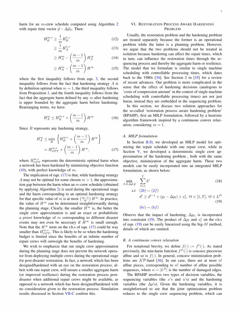
VI. RESTORATION PROCESS AWARE HARDENINGPROBLEM

Usually, the restoration problem and the hardening problemare treated separately because the former is an operationalproblem while the latter is a planning problem. However,we argue that the two problems should not be treated inisolation because hardening can affect the repair times, whichin turn, can influence the restoration times through the se-quencing process and thereby the aggregate harm or resilience.The model that we formulate is similar to single machinescheduling with controllable processing times, which datesback to the 1980s [34]. See Section 2 in [35] for a reviewof recent advances. Our problem is more complicated in thesense that the effect of hardening decisions (analogous to‘costs of compression amount’ in the context of single machinescheduling with controllable processing times) are not justlinear, instead they are embedded in the sequencing problem.

In this section, we discuss two solution approaches forthe so-called ‘restoration process aware hardening problem’(RPAHP), first an MILP formulation, followed by a heuristicalgorithm framework inspired by a continuous convex relax-ation, considering m = 1.

A. MILP formulation

In Section II-D, we developed an MILP model for opti-mizing the repair schedule with one repair crew, while inSection V, we developed a deterministic single crew ap-proximation of the hardening problem , both with the sameobjective, minimization of the aggregate harm. These twomodels can be easily incorporated into an integrated MILPformulation, as shown below:

min~x,~u,∆~p,~y

T∑t=1

ht (18)

s.t (2b) ∼ (2f)

dt ≥ dt−1 + (pl −∆pl)× xtl , ∀t ∈ [1, T ], ∀l ∈ LD(19)

(6c) ∼ (6f)

Observe that the impact of hardening, ∆pl, is incorporatedinto constraint (19). The product of ∆pl and xtl on the r.h.sof eqn. (19) can be easily linearized using the big-M method,details of which are omitted.

B. A continuous convex relaxation

For notational brevity, we define f(·) := f1(·). As statedpreviously, the min-harm function fm(·) is concave piecewiseaffine and so is f(·). In general, concave minimization prob-lems are NP-hard [36]. In our case, there are at most n!affine pieces, corresponding to n! number of affine possiblesequences, where n = |LD| is the number of damaged edges.

The RPAHP involves two types of decision variables, thesequencing variables (the x’s and u’s) and the hardeningvariables (the ∆p’s). Given the hardening variables, it isstraightforward to see that the joint optimization problemreduces to the single crew sequencing problem, which can

8

be solved optimally in polynomial time as stated previouslyin Section II-D.

Now let us consider the case where the sequencing variablesare fixed. Let Ωl :=

∑j∈Rl

wj , where Rl is the set of someedges l ∈ LD and all its successors in the given sequence.The quantity Ωl represents the reduction in aggregate harm perunit decrease in pl. The objective function for the hardeningproblem can now be recast as f(~p) =

∑l∈LD Ωl pl, which

implies:

f(~p−∆~p) =∑l∈LD

Ωlpl −∑l∈LD

Ωl∆pl (20)

Since the first term on the r.h.s of eqn. (20) is a constant,instead of minimizing f(~p − ∆~p), an equivalent formulationis:

max~y

∑l∈LD

∑k∈Kl

Ωl∆plkylk (21a)

s.t.∑k∈Kl

ylk ≤ 1 ,∀l ∈ LD (21b)∑l∈LD

∑k∈Kl

clkylk ≤ C (21c)

ylk ∈ 0, 1, ∀l ∈ LD, ∀k ∈ Kl (21d)

This model is similar to that of the multiple choice knapsackproblem [31], where Ωl∆plk’s are the value coefficients andclk’s are the cost coefficients. Since the multiple choiceknapsack is known to be NP-hard, we propose an algorithmbased on convex envelopes and LP relaxation, similar to [37].

Definition 2 (Convex envelope [38]). Let M ⊂ Rn be convexand compact and let g : M → R be lower continuous on M .A function g : M → R is called the convex envelope of f onM if it satisfies:

• g(x) is convex on M ,• g(x) ≤ g(x) for all x ∈M ,• there is no function h : M → R satisfying (1), (2) andg(x0) < h(x0) for some point x0 ∈M .

Intuitively, the convex envelope is the best underestimatingconvex function of the original function. Details of a polyno-mial time algorithm for computing the convex envelope of apiecewise linear function can be found in [37].

Given a discrete function of clk vs. ∆plk for some edgel and a set of all hardening actions k ∈ Kl, we firstconnect the neighboring points, starting from the origin, toconstruct a continuous piecewise linear cost function Cl(∆pl),where ∆pl is the relaxed continuous decision variable. Itfollows from Assumption 1 that Cl is a strictly increasingfunction. Let Cl denote the convex envelope of Cl andKl = 1, 2, · · · , |Kl| denote the set of breakpoints/knots onthe convex envelope (excluding the origin) corresponding tothe hardening strategies in consideration, indexed in ascendingorder of ∆plk. The linear relaxation of (21) based on the

convex envelope approximations, which we denote as (LP),can then be formulated as:

max∆~p

∑l∈LD

Ωl∆pl (22a)

s.t. Ql ≥ maxk∈Kl

[µlk (∆pl − αlk) + blk] , ∀l ∈ LD (22b)∑l∈LD

Ql ≤ C (22c)

0 ≤ ∆pl ≤ ∆pl,|Kl|, ∀l ∈ LD (22d)

where µlk and blk are the slope and intercept of the kth pieceof Cl, αlk is the lower breakpoint of the kth piece of Cl,and Ql is an intermediate decision variable which accountsfor the budget spent on edge l. This formulation is similar tothe conventional continuous knapsack problem, and it turnsout that the optimal values of ∆pl are always from the set0, some βlk, (αlk, βlk), where βlk is the upper breakpoint ofthe kth piece of Cl. Furthermore, at most one ∆pl can havean intermediate value in the range (αlk, βlk) in the optimalsolution. For some l and k > 1, the intercept parameter, blk, is:blk = Cl (αlk) = Cl

(βl(k−1)

). For k = 1, αlk = Cl (αlk) =

blk = 0.The preceding LP relaxation (22) can also be solved op-

timally using a greedy algorithm by first sorting the ratiosΩl

µlk

in a descending order, and then choosing the compo-

nents (and the degree of hardening) based on that sorted listiteratively, until the budget is exhausted. Ties, if any, duringthe selection process, are broken arbitrarily. We use a ∆pvariable for each edge l and each segment k of Cl. All these∆plk variables are initialized to 0. Once a selection is madefrom the sorted list at any iteration T , say (lT , kT ), we set∆plT kT equal to the maximum value possible within the range[αlT kT , βlT kT ] such that the ‘cumulative budget’ at the endof iteration T does not exceed C. Typically, this maximumvalue will be at the upper breakpoint βlT kT , unless, doingso results in a budget violation. In that case, a proper valuewithin the range (αlT kT , βlT kT ) is chosen such that the budgetis met exactly. At the end of every iteration, we evaluate theexpression of budget spent:

Λ =∑l∈LD

Cl

(maxk∈Kl

∆plk), (23)

which represents the cumulative budget consumed till thecurrent iteration. The algorithm terminates when Λ = C. Upontermination, the optimal ∆pl values can be obtained from the∆plk values as follows:

∆pl = maxk∈Kl

∆plk . (24)

The optimality of the greedy algorithm for solving the LPrelaxation (22) using the convex envelopes of the hardeningcost functions is proven in the appendix of [39].

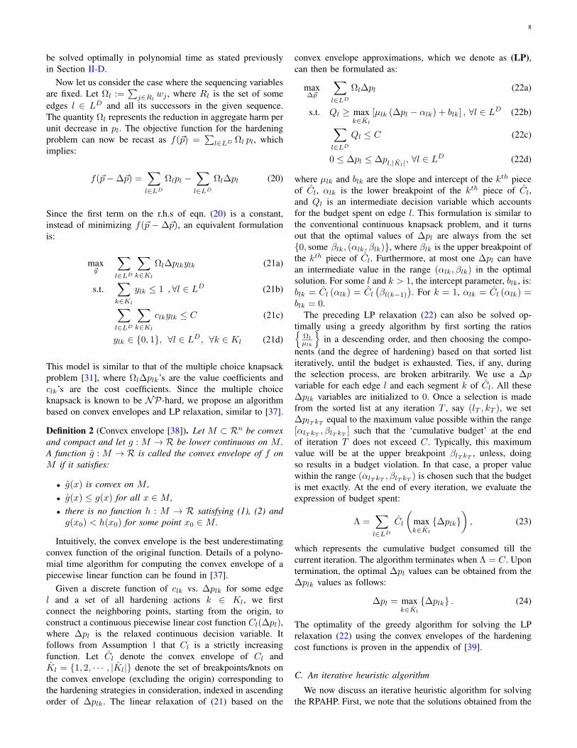
C. An iterative heuristic algorithm

We now discuss an iterative heuristic algorithm for solvingthe RPAHP. First, we note that the solutions obtained from the

9

greedy algorithm used to solve the convex relaxation formu-lation (22) may need to be rounded down to the nearest lowerbreakpoints on the convex envelopes so that the hardeningstrategy is feasible for each edge. However, after completionof the rounding process, we may find that a portion of thebudget has been left unspent. We therefore incorporate abackfill heuristic which iteratively solves LP relaxations of theform (22) with the unspent budget from the previous iterationand the remaining available hardening options, along withupdated convex envelopes, followed by a rounding down toa feasible hardening strategy. The backfill process terminateswhenever the budget has been spent exactly, or, when nofurther enhancement is possible on any edge without exceedingthe budget. Fig. 5 provides a flowchart of the iterative heuristicalgorithm for solving the restoration process aware hardeningproblem. An illustrative example can be found in [39].

Calculate schedule by Algorithm 1 and Ω𝑙 ’s accordingly

Obtain(update) convex

envelope 𝐶𝑙(∆𝑝𝑙) for each line 𝑙

Solve linear relaxation (LP) by greedy algorithm

Round LP solution ∆𝑝𝑙’s to nearest lower

knot

Budget spent or actions

depleted?

SolutionYes

No

Update remaining budget 𝐶, available

options ∆𝑝𝑙𝑘

Fig. 5: Flowchart of an iterative heuristic algorithm for solvingthe RPAHP.

VII. CASE STUDIES

A. IEEE 13 node test feeder

We first tested the MILP and the heuristic approach dis-cussed in the previous section on the IEEE 13 node testfeeder with randomly generated Cl’s and two different bud-gets. Values of E[f(·)] in this section were computed usingMonte Carlo simulations assuming an independent geometricdistribution for each pl. With a budget of C = 20, hardeningactions did not result in different repair schedules and boththe MILP and heuristic approaches yielded identical results.With a budget of C = 60, even though the hardening actionssuggested by the MILP and heuristic approaches differ fortwo edges, as shown in Table I, the objective values obtainedfrom the greedy algorithm, both for E[f(·)] and its upperbound f(E[·]), are very close to those provided by the MILPformulation. In fact, the ratios of the f(E[·]) measure from

the greedy algorithm to the E[f(·)] measure from the MILPalgorithm are both approximately 1.04 for C = 20 and C = 60(note that this ratio captures the worst case performance loss,including the effect of upper bounding the true objectivefunction using Jensen’s inequality).

TABLE I: Comparison of hardening results on the IEEE 13node test feeder with a budget of C = 60.

Edge l ∆pl by MILP ∆pl by heuristic671-684 0.2 0.4645-646 0 0.4632-645 0.5 0.8632-671 5.3 3.5f(E[·]) 14.411 14.520

E[f(·)] 13.987 14.146

We then varied the hardening budget from 0 to 50. Fig. 6shows the aggregate harm as a function of the budget form = 1. The MILP and the heuristic produced almost identicalresults when using the f(E[·]) measure so that their plotsalmost overlap. The plots corresponding to the E[f(·)] measureare also very close, considering the errors introduced by MonteCarlo simulations. The gap between the true objective and thedeterministic objective, E[f(·)]−f(E[·]), is fairly constant forboth the MILP and the heuristic. As expected, the aggregateharm decreases (resilience increases) as the hardening budgetincreases.

15

16

17

0 10 20 30 40 50

Budget

Agg

rega

teha

rm

Objectives byalgorithmsf(E[·]) by Heuristicf(E[·]) by MILPE[f(·)] by HeuristicE[f(·)] by MILP

Fig. 6: Aggregate harm vs. hardening budget for the IEEE 13node test feeder.

Finally, in Fig. 7, we compare the pre-hardening sequencingdecisions with the post-hardening decisions calculated usingthe MILP for the same case study as in Table I. In theseGantt charts, each ‘box’ represents the repair of a line andthe width of each ‘box’ is proportional to the repair time,appropriately scaled for better visualization. Observe that thetwo sequences differ by the relative locations of lines (632,645), (645, 646) and (632, 633). This confirms the interactionbetween sequencing and hardening decisions. Finally, we wantto emphasize that these sequencing decisions are abstractconstructs that only serve to model operational decisions atthe planning stage.

B. IEEE 37 node test feeder

Next, we ran our algorithms on one instance of the IEEE37 node test feeder [40]. Since the running time of the MILP

10

(633,634)(692,675)(671,680)(671,692)(684,652)(684,611)(671,684)(632,671)(632,633)(645,646)(632,645)(650,632)

(a) Gantt chart of sequencing decisions before hardening

(633,634)(692,675)(671,680)(671,692)(684,652)(684,611)(671,684)(632,671)(645,646)(632,645)(632,633)(650,632)

(b) Gantt chart of sequencing decisions after hardening (MILP)

Fig. 7: Comparison of optimal single crew repair schedules before and after hardening.

formulation increases exponentially with network size, weallocated a time budget of 10 hours. In contrast, the heuristicalgorithm yielded a solution within seconds. Table II showsthe edges for which the MILP and heuristic approach produceddifferent hardening results, along with the objective functionvalues.

TABLE II: Comparison of hardening results, ∆pl’s, on theIEEE 37 node test feeder with C = 200.

Edge l ∆pl by MILP(10 hours) ∆pl by heuristic744-729 0.8 0708-733 0 0.3702-705 2.1 0.4708-732 0 0.2734-710 0.1 1.4f(E[·]) 843.08 842.04

E[f(·)] 672.21 667.35

Analogous to Fig. 6, Fig. 8 shows a plot of the aggregateharm vs. the hardening budget for m = 1. Due to theinordinate amount of time required to solve the MILP, weshow results only for the heuristic. Unlike the 13 node feeder,the aggregate harm in this case exhibits a steep drop initiallybefore gradually tapering off. This tapering off reflects the factthat our cost functions were so chosen that no line could behardened enough to reduce its repair time to zero; i.e., forevery line l, we ensured that pl −∆pl > 0.

300

600

900

1200

0 250 500 750 1000

Budget

Agg

rega

teha

rm

Objectives byalgorithmsf(E[·]) by HeuristicE[f(·)] by Heuristic

Fig. 8: Aggregate harm vs. hardening budget for the IEEE 37node test feeder.

C. IEEE 8500 node test feeder

Finally, we tested the performance of the heuristic algorithmon one instance of the IEEE 8500 node test feeder medium

voltage subsystem [41] containing roughly 2500 edges. Wedid not attempt to solve the ILP model in this case, butthe heuristic algorithm took just 9.36 seconds to solve thisproblem.

Analogous to Figs. 6 and 8, Fig. 9 shows a plot of theaggregate harm vs. the hardening budget for m = 1. Due toissues with computational time, we chose to plot the f(E[·])measure only as a function of the budget using the heuristicalgorithm.

6.4e+06

6.6e+06

6.8e+06

7.0e+06

0 500 1000 1500 2000Budget

f(E

[·])

bygr

eedy

algo

rith

m

Fig. 9: Aggregate harm vs. hardening budget for the IEEE8500 node test feeder.

Even if hardening decisions at the planning stage are madebased on single crew operational scheduling, the resilience ofthe system would still improve if multiple crews are deployedat the operational stage. To emphasize this aspect, Fig. 10shows the normalized improvement in harm,

β :=Hm −Hm

A

Hm(25)

for different values of m. The reduction in the repair timevector due to hardening, ∆~pA, was obtained using the iterativeheuristic algorithm with a budget of C = 2000. For m > 1,the aggregate harms before and after hardening, Hm andHmA , were determined from m-crew schedules obtained using

Algorithm 2. The normalized improvement in harm shows aslight decrease (note the scale on the y-axis). This generallydecreasing trend is understandable since the improvementin system resilience due to the availability of an increasingnumber of repair crews will gradually outweigh the improve-ment in resilience due to hardening with a limited budget.Nevertheless, even for m = 50, we can observe that thenormalized improvement in harm due to hardening remainsabove 8%, even though the hardening decisions were madeconsidering m = 1.

11

0.085

0.086

0.087

0 10 20 30 40 50

Number of repair crews m

Impr

ovem

ent

ofha

rmβ

Fig. 10: Normalized improvement in harm, β (see eqn. 25),as a function of the number of repair crews, m, for the IEEE8500 node test feeder.

VIII. CONCLUSIONS

In this paper, we investigated the problem of strategicallyhardening a distribution network to be resilient against naturaldisasters. Motivated by research on resilient infrastructure sys-tems in civil engineering, we proposed an equivalent definitionof resilience with a clear physical interpretation. This allowsus to integrate the post disaster restoration process and theplanning stage component hardening decision process into oneproblem, which, we argued, is necessary since both aspectsultimately contribute to system resilience. This is a majordeparture from most current research where the two aspectsof resilience are treated separately. We first modeled therestoration problem as an MILP and the hardening problem asa stochastic program, which was reformulated using Jensen’sinequality and approximated by single crew for computationaltractability. Finally, we unified the sequencing and hardeningaspects and proposed an integrated MILP model as wellas an iterative heuristic algorithm. The expected componentrepair times are used to generate an optimal single crewrepair sequence, based on which hardening decisions are madesequentially in a greedy manner. Simulations on IEEE standardtest feeders show that the heuristic approach provides near-optimal solutions efficiently even for large networks.

REFERENCES

[1] NERC, “Hurricane sandy event analysis report.” http://www.nerc.com/pa/rrm/ea/Oct2012HurricanSandyEvntAnlyssRprtDL/Hurricane_Sandy_EAR_20140312_Final.pdf, January 2014. [Online; accessed11-March-2018].

[2] A. Kwasinski, J. Eidinger, A. Tang, and C. Tudo-Bornarel, “Performanceof electric power systems in the 2010 - 2011 Christchurch, New Zealand,Earthquake Sequence,” Earthquake Spectra, vol. 30, no. 1, pp. 205–230,2014.

[3] Infrastructure Security and Energy Restoration, Office of Electricity De-livery and Energy Reliability, U.S. Department of Energy, “A Review ofPower Outages and Restoration Following the June 2012 Derecho.” http://energy.gov/sites/prod/files/Derecho%202012_%20Review_0.pdf, Aug2012. [Online; accessed 11-March-2018].

[4] Washington, DC: Executive Office of the President,“Economic benefits of increasing electric grid resilienceto weather outages.” https://www.energy.gov/downloads/economic-benefits-increasing-electric-grid-resilience-weather-outages,2013. [Online; accessed 11-March-2018].

[5] The GridWise Alliance, “Improving electric grid reliabilityand resilience: Lessons learned from superstorm sandy andother extreme events.” http://www.gridwise.org/documents/ImprovingElectricGridReliabilityandResilience_6_6_13webFINAL.pdf,July 2013. [Online; accessed 11-March-2018].

[6] Y. Tan, F. Qiu, A. K. Das, D. S. Kirschen, P. Arabshahi, and J. Wang,“Scheduling Post-Disaster Repairs in Electricity Distribution Networks,”ArXiv e-prints arXiv:1702.08382, Feb. 2017.

[7] S. G. Nurre, B. Cavdaroglu, J. E. Mitchell, T. C. Sharkey, and W. A.Wallace, “Restoring infrastructure systems: An integrated network de-sign and scheduling (INDS) problem,” European Journal of OperationalResearch, vol. 223, no. 3, pp. 794–806, 2012.

[8] C. Coffrin and P. Van Hentenryck, “Transmission system restoration:Co-optimization of repairs, load pickups, and generation dispatch,” inPower Systems Computation Conference, 2014, pp. 1–8, IEEE, 2014.

[9] M. Omer, The Resilience of Networked Infrastructure Systems: Analysisand Measurement, vol. 3. World Scientific, 2013.

[10] M. Rollins, “The hardening of utilitiy lines-implications for utilitypole design and use.” http://woodpoles.org/portals/2/documents/TB_HardeningUtilityLines.pdf, 2007. [Online; accessed 25-March-2018].

[11] L. Mili and N. V. Center, “Taxonomy of the characteristics of powersystem operating states,” in 2nd NSF-VT Resilient and SustainableCritical Infrastructures (RESIN) Workshop, Tucson, AZ, Jan, pp. 13–15, 2011.

[12] O’Rourke, Thomas D, “Critical infrastructure, interdependencies, andresilience,” The Bridge, vol. 37, no. 1, p. 22, 2007.

[13] Electric Power Research Institute, “Enhancing Distribution Resiliency:Opportunities for Applying Innovative Technologies,” pp. 1–20, Jan.2013.

[14] B. Obama, “Preparing the united states for the impacts of climatechange,” Executive Order, vol. 13653, pp. 66819–66824, 2013.

[15] National Infrastructure Advisory Council, “A frameworkfor establishing critical infrastructure resilience goals: Finalreport and recommendations.” https://www.dhs.gov/publication/niac-framework-establishing-resilience-goals-final-report, July 2010.[Online; accessed 25-March-2018].

[16] D. A. Reed, K. C. Kapur, and R. D. Christie, “Methodology forAssessing the Resilience of Networked Infrastructure,” IEEE SystemsJournal, vol. 3, pp. 174–180, June 2009.

[17] G. Brown, M. Carlyle, J. Salmerón, and K. Wood, “Defending criticalinfrastructure,” Interfaces, vol. 36, no. 6, pp. 530–544, 2006.

[18] V. M. Bier, E. R. Gratz, N. J. Haphuriwat, W. Magua, and K. R.Wierzbicki, “Methodology for identifying near-optimal interdictionstrategies for a power transmission system,” Reliability Engineering &System Safety, vol. 92, no. 9, pp. 1155–1161, 2007.

[19] W. Yuan, L. Zhao, and B. Zeng, “Optimal power grid protection througha defender–attacker–defender model,” Reliability Engineering & SystemSafety, vol. 121, pp. 83–89, 2014.

[20] W. Yuan, J. Wang, F. Qiu, C. Chen, C. Kang, and B. Zeng, “Robustoptimization-based resilient distribution network planning against natu-ral disasters,” IEEE Transactions on Smart Grid, vol. 7, no. 6, pp. 2817–2826, 2016.

[21] S. Ma, B. Chen, and Z. Wang, “Resilience enhancement strategy fordistribution systems under extreme weather events,” IEEE Transactionson Smart Grid, 2016.

[22] E. Yamangil, R. Bent, and S. Backhaus, “Resilient upgrade of electri-cal distribution grids,” in Twenty-Ninth AAAI Conference on ArtificialIntelligence, 2015.

[23] H. Nagarajan, E. Yamangil, R. Bent, P. Van Hentenryck, and S. Back-haus, “Optimal resilient transmission grid design,” in Power SystemsComputation Conference (PSCC), 2016, pp. 1–7, IEEE, 2016.

[24] N. Romero, L. K. Nozick, I. Dobson, N. Xu, and D. A. Jones, “Seismicretrofit for electric power systems,” Earthquake Spectra, vol. 31, no. 2,pp. 1157–1176, 2015.

[25] Y. Wang, C. Chen, J. Wang, and R. Baldick, “Research on resilience ofpower systems under natural disasters - a review,” Power Systems, IEEETransactions on, vol. PP, no. 99, pp. 1–10, 2015.

[26] E. Yamangil, R. Bent, and S. Backhaus, “Designing resilient electricaldistribution grids,” Proceedings of the 29th Conference on ArtificialIntelligence, Austin, Texas, 2015.

[27] D. Adolphson and T. C. Hu, “Optimal linear ordering,” SIAM Journalon Applied Mathematics, vol. 25, no. 3, pp. 403–423, 1973.

[28] P. Brucker, Scheduling algorithms, vol. 3. Springer, 2007.[29] A. Patton, “Probability distribution of transmission and distribution

reliability performance indices,” in Reliability Conference for ElectricPower Industry, pp. 120–122, 1979.

12

[30] R. Billinton and E. Wojczynski, “Distributional variation of distributionsystem reliability indices,” IEEE Transactions on Power Apparatus andSystems, no. 11, pp. 3151–3160, 1985.

[31] P. Sinha and A. A. Zoltners, “The multiple-choice knapsack problem,”Operations Research, vol. 27, no. 3, pp. 503–515, 1979.

[32] J. L. W. V. Jensen, “Sur les fonctions convexes et les inégalités entreles valeurs moyennes,” Acta mathematica, vol. 30, no. 1, pp. 175–193,1906.

[33] S. Simic, “On a global upper bound for Jensen’s inequality,” Journal ofMathematical Analysis and Applications, vol. 343, no. 1, pp. 414–419,2008.

[34] E. Nowicki and S. Zdrzałka, “A survey of results for sequencing prob-lems with controllable processing times,” Discrete Applied Mathematics,vol. 26, no. 2-3, pp. 271–287, 1990.

[35] A. Shioura, N. V. Shakhlevich, and V. A. Strusevich, “Application ofsubmodular optimization to single machine scheduling with controllableprocessing times subject to release dates and deadlines,” INFORMSJournal on Computing, vol. 28, no. 1, pp. 148–161, 2016.

[36] M. R. Garey, D. S. Johnson, and L. Stockmeyer, “Some simplified NP-complete graph problems,” Theoretical computer science, vol. 1, no. 3,pp. 237–267, 1976.

[37] S. Kameshwaran and Y. Narahari, “Nonconvex piecewise linear knap-sack problems,” European Journal of Operational Research, vol. 192,no. 1, pp. 56–68, 2009.

[38] R. Horst and H. Tuy, Global optimization: Deterministic approaches.Springer Science & Business Media, 2013.

[39] Y. Tan, A. K. Das, P. Arabshahi, and D. S. Kirschen, “Distribu-tion Systems Hardening against Natural Disasters,” ArXiv e-printsarXiv:1711.02205, Nov. 2017.

[40] W. H. Kersting, “Radial distribution test feeders,” in 2001 IEEE PowerEngineering Society Winter Meeting. Conference Proceedings (Cat.No.01CH37194), vol. 2, pp. 908–912 vol.2, 2001.

[41] R. F. Arritt and R. C. Dugan, “The IEEE 8500-node test feeder,” inIEEE PES Transmission and Distribution Conference and Exposition,pp. 1–6, April 2010.

Yushi Tan received the B.S. degree from the Electri-cal Engineering Department of Tsinghua Universityin China, in 2013. He is currently pursuing Ph.D.degree in the University of Washington, Seattle, WA,USA. His research interests include power systemresilience under natural disasters.

Arindam K. Das received his M.S and Ph.D in Elec-trical Engineering from the Univ. of Washington,Seattle, in 1999 and 2003 respectively. From 2003to 2007, he was a post doctoral research associatejointly with the Dept. of Electrical Eng. and theDept. of Aeronautics and Astronautics, Univ. ofWashington, Seattle. From 2007 t0 2012, he workedas a Research Scientist at the Applied Physics Labo-ratory, Univ. of Washington, Seattle. He is currentlyan Assistant Professor in Electrical Engineering atEastern Washington University, Cheney, WA and an

Affiliate Assistant Professor in Electrical Engineering at the Univ. of Washing-ton, Seattle. He is also an independent consultant to several technology andbiotech companies. His current research interests are broadly in the areasof optimization theory and applications, machine learning, meta-heuristicoptimization, and wireless networking.

Payman Arabshahi received his M.S. and PhDin Electrical Engineering from the University ofWashington in 1990 and 1994 respectively. He iscurrently Associate Professor, and Associate Chairfor Advancement at the University of Washington’sDepartment of Electrical Engineering; Faculty Leadof Innovation Training at UWâAZs Collaborative In-novation Hub (CoMotion); and a principal researchscientist with the UW Applied Physics Laboratory.From 1994-1996 he served on the faculty of theElectrical and Computer Engineering Department at

the University of Alabama in Huntsville. From 1997-2006 he was on thesenior technical staff of NASAâAZs Jet Propulsion Laboratory, in the Com-munications Architectures and Research Section, working on Earth orbit anddeep space communication networks and protocols, and design of planetaryexploration missions. While at JPL he also served as affiliate graduate facultyat the Department of Electrical Engineering at Caltech, where he taught thethree-course graduate sequence on digital communications. He has been aguest editor of the IEEE Transactions on Neural Networks; and most recently,General Co-Chair of the 11th ACM International Conference on UnderwaterNetworks & Systems in Shanghai. He has been the co-founder of, or advisorto, a number of technology startups. His interests are in entrepreneurshipeducation, underwater and space communications, wireless networks, datamining and search, and signal processing.

Daniel Krischen (M’86-SM’91-FâAZ07) is theDonald W. and Ruth Mary Close Professor of Elec-trical Engineering at the University of Washington.Prior to joining the University of Washington, hetaught for 16 years at The University of Manchester(UK). Before becoming an academic, he workedfor Control Data and Siemens on the developmentof application software for utility control centers.He holds a PhD from the University of Wisconsin-Madison and an Electro-Mechanical Engineering de-gree from the Free University of Brussels (Belgium).