distributed parallel power system...
TRANSCRIPT

Distributed Parallel Power System Simulation
Mike Zhou Ph.D.
Chief Architect, InterPSS Systems
Canton, MI, USA
Abstract The information technology (IT) world has changed fundamentally and
drastically from running software applications on a single computer with a single
CPU to now running software as services in distributed and parallel computing
environment. Power system operation has been also shifted from being solely
based on off-line planning study to more and more real-time market-driven. Fac-
ing these challenges, we will discuss in this chapter how to design power system
analysis and simulation software to take advantage of the new IT technologies and
to meet the real-time application requirements, using the InterPSS project as a
concrete example.
1. Introduction
Due to technology advance, business competiveness and regulation changes, it is
becoming more and more demanded to carry out large amount of computation in
real-time in power system operation. The author started power system simulation
programming 30 years ago, when studying as a PhD student at Tsinghua Universi-
ty (Beijing, China). In 1985, China was planning to build the Three Gorges Power
Plant, which would be the largest hydro power plant in the world. At that time,
there was no commercial packaged power system simulation software available in
China. The author was assigned the task to develop a power system simulation
program for the feasibility study, including loadflow, short circuit and transient
stability with HVDC transmission lines. The simulation program was completed
in about 3 months and used for the study. It was written in FORTRAN language in
the procedure programming style, and running then on a single computer with a
single Central Processing Unit (CPU).
The information technology world has changed fundamentally and drastically
since then. Today, a typical enterprise computing environment consists of a set,
sometime a farm, of computers connected by high-speed and reliable computer
networks. The computers are usually equipped with multiple multi-core proces-
sors, capable of running many, sometimes massive numbers of, computation tasks
2
in parallel to achieve highly-available and fault-tolerant computations. Distributed
and parallel computing is the foundation for today’s highly-available SOA (Ser-
vice-Oriented Architecture) enterprise computing architecture.
Also, the way how power system is operated has changed from planned to real-
time and market-driven. Power system operations used to be planned according to
the off-line planning study many months ahead. Today, power system operations
are moving to market-driven, allowing transmission of power from one node to
another to be arranged real-time on-demand by the market participants. High per-
formance computing (HCP) technology-based real-time power system analysis
tools will play a more and more import role to ensure reliability and stability of fu-
ture power system operations.
1.1 Challenges
Instead of increasing the CPU clock speed and straight-line instruction through-
put, the computer industry is currently turning to the multi-core processor archi-
tecture and the distributed computing approach for high performance computing
(HPC). The amount of performance gain by the use of a multi-core processor de-
pends very much on the software algorithms and implementation. In particular, the
possible gains are limited by the fraction of the software that can be parallelized to
run on multiple cores/CPU/computers simultaneously. Therefore distributed and
parallel computing is one of the most important issues, which needs to be ad-
dressed, for today and tomorrow’s HPC in power and energy systems.
For those who wrote FORTRAN code for power system analysis and simulation
before, the following code snippet might not be foreign:
INTEGER N, BusNo(10000) REAL P(10000), Q(10000) (1) COMMON /BUSDATA/ N, BusNo, P, Q
where, N is the number of buses; BusNo bus number array; and P,Q for storing bus
p and q. BUSDATA is a common data block for passing data between subroutines,
which is accessible globally in the application. There are at least two major prob-
lems when trying to run the above code in a distributed and parallel computing
environment.
1.1.1 Multi-thread Safe
The objective of parallel computing is to reduce the overall computation time of
a computation task by dividing the task into a set of subtasks (simulation jobs) that
can be processed independently and concurrently. Multiple subtasks can concur-
3
rently read the same memory location (the common data black), which is shared
among them. However, concurrent writes to the same memory location generated
by multiple subtasks would create conflicts. The order in which the subtasks
would perform their write is non-deterministic, making the final state unpredicta-
ble. In computer science, the common data block is called static global variable. It
has been a known fact that using static global variable makes the code multi-
thread unsafe. Therefore the above code set (1) could not be safely executed in a
computation process in parallel without causing data integrity issues, because of
the common data block usage.
1.1.2 Serialization/de-serialization
In distributed computing, there are often situations where application informa-
tion in the memory of a computer, needs to be serialized and sent to another com-
puter via the network. On the receiving end at the target computer, the serialized
information needs to be de-serialized to reconstruct the original data object graph
in the memory to continue the application logic execution. For example, for a mis-
sion-critical software application process, if an active computer running the appli-
cation crashes for some reason, the application process is required to be migrated
to a backup computer and continue the execution there. This is the so-called fault-
tolerance design. One of the key requirements for a successful fault-tolerant im-
plementation is that the information in the memory used by an application process
should be able to be easily and seamlessly serialized and de-serialized. Using the
above coding style (1), in large-scale power system simulation software, as one
can imagine, there might be hundreds or even thousands of individual variables
and arrays, scattered over many places. Serializing these variables and arrays in
the memory, and then de-serialized to re-construct the data object graph at a dif-
ferent computer would be extremely difficult, if not impossible.
1.2 Near Real-time Batch Processing
In computer science, a thread of execution is the smallest unit of processing that
can be scheduled by a computer’s operating system. A thread is contained inside a
computer application process. Multiple threads can co-exist within the same appli-
cation process and share resources such as the memory, while different processes
cannot share these resources. In general, threads are “cheap” and application
processes are “expensive”, in terms of system resources usage. A parallel power
system simulation approach was presented in [Lin, 2006], where a job scheduler is
used to start multiple single-thread application processes to perform power system
simulation in parallel. It is a known fact among computer science professionals

4
that this kind of approach, which is sometimes called near real-time batch
processing, is not efficient and has many side-effects.
"We argue that objects that interact in a distributed system need to be dealt with
in ways that are intrinsically different from objects that interact in a single address
space. ... Further, work in distributed object-oriented systems that is based on a
model that ignores or denies these differences is doomed to failure, and could easi-
ly lead to an industry-wide rejection of the notion of distributed object-based sys-
tems."[Waldo 2004] In our opinion, FORTRAN, along with other procedural pro-
gramming language-based legacy power system software packages, which were
designed to function properly on a single computer with a single CUP (single ad-
dress space), in general cannot be evolved and adapted to take full advantage of
the modern multi-processor, multi-core hardware architecture and the distributed
computing environment. The legacy power system simulation software packages
cannot be easily deployed in, and able of taking advantage of, today’s highly-
available enterprise computing environment.
1.3 InterPSS Project
The discussion material presented in this chapter is based on an actual power
system simulation software implementation – the InterPSS project [Zhou 2005].
The question, the InterPSS development team want to address, is not so much how
to develop or adapt a distributed parallel computing system to run some existing
legacy power system simulation software, but rather on how to develop a com-
pletely new power system simulation engine in certain way and with certain fea-
tures, that will enable it to run in most modern enterprise computing environments
available today, and being able to be adapted to possible future HPC innovations.
The InterPSS project is based on modern software development methodology,
using the object-oriented power system simulation programming approach [Zhou,
1996] and Java programming language, with no legacy FORTRAN code. Its open
and loosely coupled software architecture allows components developed by others
to be easily plugged into the InterPSS platform to augment its functionalities or al-
ter its behaviors, and equally important, allows its components to be integrated in-
to other software systems. The project is currently developed and maintained by a
team of developers living in the United States and China.
In summary, the focus of this chapter is not on a particular distributed and parallel
computing technology, but rather on how to architect and design power system
analysis and simulation software to run in modern distributed and parallel compu-
ting environment to achieve high performance.

5
2. Power System Modeling
Power system simulation software, except for those targeted for university teach-
ing or academic research, is very complex and usually takes years to develop.
When starting a large-scale software development project, the first important step
is to study how to model the problem which the software is attempted to solve.
This section discusses power system modeling from power system analysis and
simulation perspective. A model, in the most general sense, is anything used in
any way to represent anything else. There are different types of models for differ-
ent purposes.
• Physical model - Some models are physical, for instance, a transformer model
in a physical power system laboratory which may be assembled and made work
like the actual object (transformer) it represents.
• Conceptual model - A conceptual model may only be drawn on paper, described
in words, or imagined in the mind, which is commonly used to help us get to
know and understand the subject matter it represents. For example, the IEC
Common Information Model (CIM) is a conceptual model for representing
power system at the physical device level.
• Concrete implementation model - A conceptual model could be implemented in
multiple ways by different concrete implementation models. For example, a
computer implementation (concrete) model is a computer software application
which implements a conceptual model.
2.1 Power System Object Model
Matrix has been used to formulate power system analysis since the computer-
based power system simulation was introduced to power system analysis. Almost
all modern power system analysis algorithms are formulated based the [Y]-matrix
- the power network Node/Branch admittance matrix. [Y]-matrix essentially is a
conceptual model representing power network for the simulation purpose. The
[Y]-matrix model has been commonly implemented in FORTRAN using one or
two dimensional arrays as the fundamental data structure. One would often find
that power system analysis software carries a label of 50K-Bus version, which re-
ally means that the arrays used in the software to store bus related data have a
fixed dimension of 50,000. This FORTRAN-style computer implementation of the
[Y]-matrix power network model has influenced several generations of power en-
gineers and been used by almost all commercial power system analysis software
packages today.
It is very important to point out that a conceptual model could be implemented
in multiple ways. This has been demonstrated by an object-oriented implementa-

6
tion of the very same power system [Y]-matrix model in [Zhou, 1996], where C++
Template-based linked list, instead of array, was used as the underlying data struc-
ture. In this implementation, a set of power system modeling vocabulary (Net-
work, Bus, and Branch) and ontology (relationship between the Network, Bus and
Branch concepts) are defined for the purpose of modeling power system for analy-
sis and simulation. The power system object model could be illustrated using the
UML – Unified Modeling Language [OMG, 2000] representation as shown in
Figure-1.
In the object model, a Bus object is a "node" to which a set of Branch objects
can be connected. A Branch object is an "edge" with two terminals which can be
connected between two Bus objects. A Network object is a container where Bus
and Branch objects can be defined, and Branch objects can be connected between
these Bus objects to form a network topology for power system simulation. In
UML terminology, [0..n] reads zero to many and [1..n] one to many. A Network
object contains [1..n] Bus objects and [1..n] Branch objects, while a Bus object
can be associated with [0..n] branches. A Branch object connects (associates) to
[1..n] Bus objects. Typically, a Branch object connects to 2 Bus objects. However,
the number might be 1 for grounding branch, or 3 for three-winding transformer.
Fig. 1 Power System Object Model
2.2 Model-based Approach
Model-driven architecture (MDA) [OMG, 2001], is a design approach for de-
velopment of software systems. In this approach, software specifications are ex-
pressed as conceptual models, which are then “translated” into one or more con-
crete implementation models that the computers can run. The translation is
generally performed by automated tools, such as the Eclipse Modeling Framework
(EMF) [Eclipse 2010]. Eclipse EMF is a modeling framework and code generation
facility for building tools and other applications based on structured data models.
From a model specification, Eclipse EMF provides tools and runtime support to
produce a set of Java classes (concrete implementation) for the model.

7
MDA–based software development approach is sometimes called model-based
approach. In this approach, the model is placed at the center of software develop-
ment and the rest evolve around the model. InterPSS uses this approach and is
based on Eclipse EMF [Zhou, 2005]. The immediate concern, one might have, is
the performance, since power system simulation is computation-intensive. For an
11865-bus test system, it took the Eclipse EMF generated Java code 1.4 sec to
load the test case data to build the model, and 15.4 sec to run a complete loadflow
analysis using the PQ method. The testing was performed on a Lenovo ThinkPad
T400 laptop. It has been concluded that the code generated by computer from the
Eclipse EMF-based power system simulation model out-performs the code ma-
nually written by the InterPSS development team. The following is a summary of
the model-based approach used by InterPSS:
• The power system simulation object model [Zhou, 2005] is first expressed in
Eclipse EMF as a conceptual model, which is easy to be understood and main-
tained by human beings.
• Using Eclipse EMF code generation, the conceptual model is turned to a set of
Java classes, a concrete implementation model, which can be used to represent
power network object model in computer memory for simulation purposes.
• The two challenges presented in Section-1.1 are addressed. Since the conceptual
model is represented by a set of UML classes, it is quite easy to change and ad-
just, to make the generated concrete implementation model multi-thread safe.
• Eclipse EMF includes a powerful framework for model persistence. Out-of-the-
box, it supports XML serialization/de-serialization. Therefore, the Eclipse EMF-
based InterPSS power system simulation object model could be serialized to and
de-serialized from Xml document automatically.
2.3 Simulation Algorithm Implementation
When the author implemented his first loadflow program about 30 years ago,
the first step was implementing loadflow algorithms, i.e., the Newton-Raphson
(NR) method and the Fast-Decoupled (PQ) method. Then, input data routines
were created to feed data into the algorithm routines. While this approach is very
intuitive and straightforward, it was found late that the program was difficult to
maintain and extend, since the program data structure was heavily influenced by
the algorithm implementation. In the model-based approach, the model is defined
and created first. The algorithm is developed after, often following the visitor de-
sign pattern, which is described below.
In software engineering, the visitor design pattern [Gamma, et al, 1994] is a way
of separating an algorithm from the model structure it operates on. A practical re-
sult of this separation is the ability to add new algorithms to existing model struc-
tures without modifying those structures. Thus, using the visitor pattern decouples

8
the algorithm implementation and the model that the algorithm is intended to ap-
ply to, and makes the software easy to maintain and evolve. The following are
some sample code, illustrating an implementation of loadflow algorithm using the
visitor pattern:
// create an aclf network object AclfNetwork aclfNet = CoreObjectFactory.createAclfNetwork(); // load some loadflow data into the network object SampleCases.load_LF_5BusSystem(aclfNet); // create an visitor - a Loadflow algorithm IAclfNetVisitor visitor = new IAclfNetVisitor() { public void visit(AclfNetwork net) { // define your algorithm here . . . } }; // run loadflow calculation by accepting the visitor visiting // the aclf network object aclfNet.accept(visitor);
The first step is to create a power system simulation object model – an
AclfNetwork object. Next, some data is loaded into the model. At this time, the
exact loadflow algorithm to be used has not been defined yet. All it says is that
necessary information for loadflow calculation have been loaded into the
simulation model object. Then a loadflow algorithm is defined as a visitor object
and loadflow calculation is performed by the visitor visiting the simulation model
object. The loadflow calculation results are stored in the model and ready to be
output in any format, for example, by yet another visitor implementation. In this
way, the power system simulation model and simulation algorithm are decoupled,
which makes it possible for the simulation algorithm to be replaced with another
implementation through software configuration using dependency injection
[Fowler 2004], see more details in the upcoming Section-3.2.
2.4 Open Data Model (ODM)
ODM [Zhou 2005] is an Open Model for Exchanging Power System Simulation
Data. The model is specified in XML using XML schema [W3C 2010]. The ODM
project, an open-source project, is currently sponsored by the IEEE Open-Source
Software Task Force. InterPSS is the ODM schema author and a main contributor
to the open-source project.
One might be familiar with the IEEE common data format [IEEE Task Force
1974]. The following is a line describing a bus record:
2 Bus 2 HV 1 1 2 1.045 -4.98 21.7 12.7 -> 40.0 42.4 132.0 1.045 50.0 -40.0 0.0 0.0 0

9
Using the ODM model, the same information could be represented in an XML
record, as follows:
<aclfBus id="Bus2" offLine="false" number="2" zoneNumber="1" areaNumber="1" name="Bus 2 HV"> <baseVoltage unit="KV" value="132.0"/> <voltage unit="PU" value="1.045"/> <angle unit="DEG" value="-4.98"/> <genData> <equivGen code="PV"> <power unit="MVA" im="42.4" re="40.0"/> <desiredVoltage unit="PU" value="1.045"/> <qLimit unit="MVAR" min="-40.0" max="50.0"/> </equivGen> </genData> <loadData> <equivLoad code="CONST_P"> <constPLoad unit="MVA" im="12.7" re="21.7"/> </equivLoad> </loadData> </aclfBus>
There are many advantages to represent data in XML format. In fact, XML cur-
rently is the de facto standard for representing data for computer processing. One
obvious benefit is that it is very easy to read by human. Anyone with power engi-
neering training can precisely interpret the data without any confusion. There is
no need to guess if the value 40.0 is generation P or load P, in PU or Mw.
The key ODM schema concepts are illustrated in Figure-2. The Network com-
plex type (NetworkXmlType) has a busList element and a branchList ele-
ment. The branch element in the complex type (branchTypeList) is of the
Branch complex type (BaseBranchXmlType). The fromBus and toBus ele-
ments are of complex type BusRefRecordXmlType, which has a reference to ex-
isting Bus record. The tertiaryBus is optional, used for 3-winding transformer.

10
Fig. 2 Key ODM Schema Concepts
IEEE common data format specification has two main sets of records – bus
record and branch record. Bus number is used to link these two sets of records to-
gether. In certain sense, it can be considered as a concrete implement model of the
[Y]-matrix model. Similarly, the key ODM schema concepts, shown in Figure-2,
are intended to describe the [Y]-matrix in an efficient way. Therefore, we can con-
sider the ODM model is another concrete implementation model of the [Y]-matrix
model.
2.5 Summary
A conceptual model could be implemented in multiple ways by different con-
crete implementation models. Power network sparse [Y]-matrix is a conceptual
model, which has been implemented in two different ways in the InterPSS project:
1) the InterPSS object model using Eclipse EMF and 2) the ODM model using
XML schema. InterPSS object model is for computer in memory representation of
power network object relationship, while the ODM model is for power network
simulation data persistence and data exchange. The relationship between these two
models and the simulation algorithms is illustrated in Figure-3. At the runtime,
power network simulation data stored in the ODM format (XML document) is
loaded into computer and mapped to the InterPSS object model. Simulation algo-
rithms, such as loadflow algorithm, are applied to the object model to perform, for
example, loadflow analysis.

11
In the model-based approach, power system simulation object model is at the
center of the software development and the rest evolve around the model in a
decoupled way, such that different simulation algorithm implementations can be
associated with the model through software configuration using the dependency
injection approach. Since the underlying data model object and the simulation
algorithms are decoupled, it is not difficult to make the data model multi-thread
safe and to implement data model serialization/de-serialization for distributed
parallel computation.
Fig. 3 Model and algorithm relationship
3. Software Architecture
The question to be addressed in this chapter is not so much about how to devel-
op a new or adapt to an existing distributed and parallel computing system to run
the legacy power system simulation software, but rather on how to architect power
system simulation software that will enable it to run in today’s enterprise compu-
ting environments, and to easily adapt to possible future HPC innovations. The
problem is somewhat similar to that on how to build a high-voltage transmission
system for scalability. When building a local power distribution system, the goal is
usually to supply power to some well-defined load points from utility source bus.
Flexibility and extensibility is not a major concern, since the number of variation
scenarios in power distribution systems is limited. When we were studying the
Three Gorges plant, there were so many unknowns and possible variation scena-
rios. In fact the plant was built more than 20 years after the initial study. At that
time, an “architecture” of parallel high-voltage HVAC and HVDC transmission
lines were suggested for reliability and stability considerations, and for flexibility
and extensibility, without knowing details of the generation equipment to be used
to build the plant and the power consumption details in the eastern China region
(the receiving end). The concept of designing scalable system architecture with
flexibility and extensibility is not foreign to the power engineering community.
In this section, the InterPSS project will be used as a concrete example to ex-
plain the basic software architecture concepts. The discussion will stay at the con-

12
ceptual level, and no computer science background is needed to understand the
discussion in this section.
Fig. 4 Comparison of Different Software Architecture
3.1 InterPSS Software Architecture
Traditional power system simulation software is monolithic with limited exten-
sion capability, as illustrated in Figure-4. InterPSS on the other hand has an open
architecture with a small core simulation engine. The other parts, including input
and output modules, user interface modules, and controller models are extension
plug-ins, which could be modified or replaced. For example, InterPSS loadflow
algorithms, sparse equation solution routines, transient stability simulation result
output modules and dynamic event handlers for transient stability simulation are
plugins, which could be taken away and replaced by any custom implementation.
InterPSS core simulation engine is very simple. It consists of the following three
parts:
• Power system object model – The power system object model discussed in Sec-
tion-2. It, in a nutshell, is a concrete implementation of the power network
sparse [Y]-matrix model (conceptual model). The implementation is in such a
generic way that it could be used or extended to represent power network for
any type of [Y]-matrix model based power system simulation.

13
• Plug-in framework – A dependency injection based plug-in framework allowing
other components, such as loadflow simulation algorithm, to be plug-in or
switched through software configuration.
• Default (replaceable) algorithm – The core simulation engine has a set of default
implementation of commonly used power system simulation algorithms, such as
loadflow Newton-Raphson method, fast-decoupled method and Gauss-Seidel
method. However, these default algorithm implementations are plug-ins, mean-
ing that they could be taken away and replaced.
InterPSS has a simple yet powerful open architecture. It is simple, since in es-
sence, it only has a generic power network sparse [Y]-matrix solver. It is power-
ful, since using the plug-in extension framework, it could be extended and used to
solve any [Y]-matrix based power system simulation problem. InterPSS core si-
mulation engine is designed to be multi-thread safe, without static global variable
usage in the power system object model. The object model, which is based on the
Eclipse EMF, could be seamlessly serialized to and de-serialized from XML doc-
ument. The core simulation engine is implemented using 100% Java with no lega-
cy FORTRAN or C code. It can run on any operating system where a Java virtual
machine (JVM) exists. It is easy to maintain since sparse [Y]-matrix for power
system simulation is well understood and is unlikely to change for the foreseeable
future, which enables the core simulation engine to be quite stable and simple to
maintain.
3.2 Dependency Injection
Dependency injection [Fowler 2004] in object-oriented programming is a design
pattern with a core principle of separating behavior from dependency (i.e., the re-
lationship of this object to any other object that it interacts with) resolution. This is
a technique for decoupling highly dependent software components. Software de-
velopers strive to reduce dependencies between components in software for main-
tainability, flexibility and extensibility. This leads to a new challenge - how can a
component know all the other components it needs to fulfill its functionality or
purpose? The traditional approach was to hard-code the dependency. As soon as a
simulation algorithm, for example, InterPSS’ loadflow implementation, is neces-
sary, the component would call a library and execute a piece of code. If a second
algorithm, for example, a custom loadflow algorithm implementation, must be
supported, this piece of code would have to be modified or, even worse, copied
and then modified.
Dependency injection offers a solution. Instead of hard-coding the dependen-
cies, a component just lists the necessary services and a dependency injection
framework supplies access to these service. At runtime, an independent compo-
nent will load and configure, say, a loadflow algorithm, and offer a standard inter-

14
face to interact with the algorithm. In this way, the details have been moved from
the original component to a set of new, small, algorithm implementation specific
components, reducing the complexity of each and all of them. In the dependency
injection terms, these new components are called "service components" because
they render a service (loadflow algorithm) for one or more other components. De-
pendency injection is a specific form of inversion of control where the concern be-
ing inverted is the process of obtaining the needed dependency.
There are several dependency injection implementations using Java program-
ming language. The Spring Framework [Spring 2010] is the most popular one,
which is used in InterPSS.
3.3 Software Extension
At the conceptual level, almost all InterPSS simulation related components
could be considered as an implementation of the generic bus I-V or branch I-V
function, as shown in Figure-5, where,
I - Bus injection or branch current;
V - Bus or branch terminal voltage;
t - Time for time-domain simulation;
dt - Time-domain simulation step.
t and dt only apply to time-domain dynamic simulation.
Fig. 5 Extension Concept
The following is a simple example to implement a constant power load (p = 1.6
pu, q = 0.8 pu) through bus object extension.
AclfBus bus = (AclfBus)net.getBus("1"); bus.setExtensionObject(new AbstractAclfBus(bus) { public boolean isLoad() { return true; } public double getLoadP() { return 1.6; } public double getLoadQ() { return 0.8; } });
The behavior of AclfBus object (id = "1") in this case is overridden by the exten-
sion object. This example, of course, is over-simplified and only for illustrating

15
the extension concept purpose. In the real-world situation, dependency injection is
used to glue custom extension code to any InterPSS simulation object to alter its
behavior.
3.4 Summary
“A good architecture is not there is nothing to add, rather nothing could be taken
away”. InterPSS has a simple yet powerful open architecture. “Change is the only
constant” is what Bill Gates said when he retired from Microsoft. The main rea-
son, such a simple yet flexible architecture is selected by the InterPSS develop-
ment team, is for the future changes and extension. InterPSS core simulation en-
gine is multi-thread safe, and its simulation object could be seamlessly
serialized/de-serialized. In the next two sections, we will discuss InterPSS exten-
sion to grid computing and cloud computing.
4. Grid Computing
InterPSS grid computing implementation will be used in this section as an exam-
ple to discuss key concepts in applying grid computing to power system simula-
tion. Until recently, mainstream understanding of computer simulation of power
system is to run a simulation program, such as a loadflow, Transient Stability or
Voltage Stability program, or a combination of such programs on a single com-
puter. Recent advance in computer network technology, and software develop-
ment methodology has made it possible to perform grid computing, where a set of
network-connected computers, forming a computational grid, located in local area
network (LAN), are used to solve certain category of computationally intensive
problems.
The Sparse matrix solution approach [Tinney, 1967] made simulation of power
system of (practically) any size and any complexity possible using a single com-
puter. The approach forms the foundation for today's computer-based power sys-
tem study. The Fast Decoupled approach [Stott, 1974] made high-voltage power
network analysis much faster. The [B]-matrix approximation concept used in the
Fast Decoupled approach forms the foundation for today’s power system on-line
real-time security analysis and assessment. However, the power engineering
community seems to agree that, by using only one single computer, it is impossi-
ble, without some sort of approximation (simplification/reduction/screening), to
meet the increasing power system real-time online simulation requirements, where
thousands of contingency analysis cases need to be evaluated in a very short pe-
riod of time using a more accurate AC loadflow power network model.

16
4.1 Grid Computing Concept
Grid computing was started at the beginning to share unused CPU cycles over
the Internet. However, the concept has been extended and applied recently to HPC,
using a set of connected computers in a LAN (Local Area Network). Google has
used grid computing successfully to conquer the Internet search challenges. We
believe grid Computing can also be used to solve power system real-time on-line
simulation problems, using the accurate AC loadflow model.
4.1.1 Split/Aggregate
The trademark of computational grids is the ability to split a simulation task into
a set of sub-tasks, execute them in parallel, and aggregate sub-results into one fi-
nal result. Split and aggregate design allows parallelizing the processes of subtask
execution to gain performance and scalability. The split/aggregate approach some-
times is called map/reduce [Dean 2004].
4.1.2 Gridgain
GridGain (www.gridgain.org) is an open-source project, providing a platform
for implementing computational grid. Its goal is to improve overall performance
of computation-intensive applications by splitting and parallelizing the workload.
InterPSS grid computing solution currently is built on top of the Gridgain plat-
form. However, the dependency of InterPSS on Gridgain is quite loose, which al-
lows InterPSS grid computing solution to be moved relative easily to other grid
computing platform in the future, if necessary.
4.2 Grid Computing Implementation
With grid computing solution, power system simulation in many cases might
not be constrained by the computation speed of a single computer with one CPU
any more. One can quickly build a grid computing environment with reasonable
cost to achieve HPC power system simulation. Using InterPSS core simulation
engine and Gridgain, a grid computing solution has been developed for power sys-
tem simulation. A typical grid computing environment setup is shown in Figure-6.
InterPSS is installed on a master node. Power system simulation jobs, such as
loadflow analysis run or transient stability simulation run, are distributed to the
slave nodes. InterPSS core simulation engine software itself is also distributed
through the network from the master node to the slave nodes one time when the
simulation starts at the slave node. InterPSS simulation model object is serialized

17
at the master node into an XML document and distributed over the network to the
remote slave node, where the XML document is de-serialized into the original ob-
ject model and becomes ready for power system simulation.
Fig. 6 Typical Grid Computing Setup
4.2.1 Terminology
The following are terminologies used in this section’s discussion:
• Slave Gird Node - A Gridgain agent instance, running on a physical computer,
where compiled simulation code can be deployed from a master grid node re-
motely and automatically through the network to perform certain simulation job.
One or more slave grid node(s) can be hosted on a physical computer.
• Master Grid Node - A computer with InterPSS grid computing edition installa-
tion. One can have multiple master grid nodes in a computation grid. Also, one
can run one or more slave grid node(s) on a master grid node computer.
• Computation Grid - One or more master grid nodes and one or many slave grid
node(s) in a LAN form an InterPSS computational grid.
• Grid Job - A unit of simulation work, which can be distributed from a master
grid node to any slave grid node to run independently to perform certain power
system simulation, such as loadflow analysis or transient stability simulation.
• Grid Task – Represent a simulation problem, which can be broken into a set of
grid jobs. Grid task is responsible to split itself into grid jobs, distribute them to
remote grid nodes, and aggregate simulation sub-results from remote grid nodes
for decision making or display purpose.

18
4.2.1 Remote Job Creation
Computer network has a finite bandwidth. Excessive communication between a
master grid node and slave grid nodes cross the network during the simulation
process may slow down the simulation. There are two ways to create simulation
jobs, as shown in Figure-7.
• Master node simulation job creation - This is the default behavior. From a base
case, simulation jobs are created at amaster node and then distributed to remote
slave nodes to perform simulation. If there are a large number of simulation
jobs, sending them in real-time through the network may take significant
amount of time and might congest the network.
• Remote node simulation job creation - In many situations, it may be more effi-
cient to distribute the base case once to remote grid nodes. For example, in the
case of N-1 contingency analysis, the base case and a list of contingency de-
scription could be sent to remote slave grid node. Then simulation job for a con-
tingency case, for example, opening branch Bus1->Bus2, can be created at a
remote slave grid node from the base case.
Fig. 7 Simulation Job Creation
19
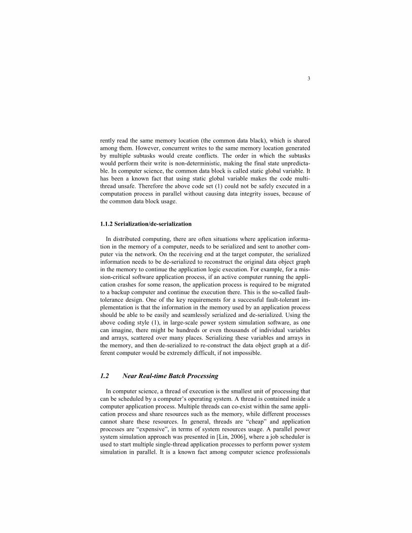
Fig. 8 InterPSS Grid Computing Performance Study
4.2.2 Performance Study
The result of an experiment by a research group at the South China University
of Technology [Hou 2009] using InterPSS grid computing is shown in Figure-8.
• loadflow study: Based on a base case of 1,245 buses and 1,994 branches, per-
form 2,500 N-1 contingency analysis by running 2,500 full AC loadflow runs in
parallel on remote grid nodes;
• Transient Stability study: Perform 1,000 transient stability simulation runs in
parallel on remote grid nodes.
The results in Figure-8 indicate that InterPSS grid computing approach can
achieve almost linear scalability, meaning doubling the computing resource (CPU)
can approximately speed-up the computation two times.
With grid computing, for certain categories of computation-intensive power sys-
tem simulation problems, where the split/aggregate technique can be used to solve
the problem in parallel, computation speed might not be the deciding or limiting
factor in selecting simulation algorithm any more. The computation speed con-
straint can be much relaxed. In the following section, an AC loadflow model and
grid computing based security assessment implementation will be discussed.
4.3 Security Assessment
Power system security assessment is the analysis performed to determine
whether, and to what extent, a power system is reasonably safe and reliable from
serious interference to its normal operation. From the power system simulation
perspective, security assessment is based on contingency analysis, which runs in
energy management system in power system control center to give the operators

20
insight on what might happen to the power system in the event of an unplanned or
un-scheduled equipment outage. Typical contingency on a power system consists
of outages such as loss of generators or transmission lines. The security assess-
ment concept and terminology, defined in [Bula 1992], are used in the following
discussion.
Real-time on-line security assessment algorithms used in today's power system
control centers are mostly designed to be run on a single computer. Because of the
computation speed limitation, most of them are based on the [B]-matrix approxi-
mation [Stott, 1974]. The following approaches are commonly used in the existing
security assessment algorithms to speed-up computation:
• Simplified model - Because of the computation speed limitation, on-line analy-
sis normally treats a power network as a DC network using [∆P] = [B]•[∆θ].
Reactive power and voltage are normally not considered in the economic dis-
patch calculation in power control center.
• Linear prediction - Linear prediction approach is commonly used to predict, for
example, the power flow increase on branch-A, if there is a branch-B outage.
Again the [B]-matrix is used to calculate the LODF - Line Outage Distribution
Factor. LODF assumes that the power network under contingency conditions
can be reasonably accurately represented by a network of impedance and con-
stant voltage sources, which is no longer accurate in today's flexible power net-
work with many electronic control and adjustment equipments, such as HVDC
transmission line, FACTS and SVC (Static Var Compensator).
• Screening - Contingency analysis requires running thousands study cases in a
short period of time, which is not feasible using a single computer and the accu-
rate AC loadflow power network model. Therefore, the common practice today
is to use some kind of screening process to pre-select a sub-set of the study cas-
es to run. The selection is normally based on sensitivity analysis using the [B]-
matrix.
The limitation of the above approaches and the need for AC Loadflow power
network model based security assessment were discussed in [Wood 1984], Sec-
tion-11.3.3. An AC loadflow model and grid computing based security assessment
has been implemented in InterPSS, including three main features: 1) N-1 contin-
gency analysis, 2) security margin computation, and 3) preventive/corrective ac-
tion evaluation.
4.3.1 N-1 Contingency Analysis
Using the grid computing approach, full AC loadflow-based contingency anal-
ysis cases are run at remote grid nodes in parallel. The analysis results are sent
back to master grid node in real-time through the network. The master grid node

21
collects all analysis results and selects the largest branch MVA flow from all con-
tingency cases for each branch to perform the security assessment.
Table-1 Branch MVA Rating Violation Report
Branch Id Mva Mva Violation Description Flow Rating ================================================================== 0001->0002(1) 241.1 200.0 21% Open branch 0001->0005 0005->0004(1) 103.2 100.0 3% Open branch 0002->0003 0006->0013(1) 51.3 50.0 3% Open branch 0007->0008 0003->0004(1) 101.2 100.0 1% Open branch 0002->0003
Table-2 Bus Voltage Security Margin
Bus Voltage Limit: [1.10, 0.90] Bus Id High V-Margin Low V-Margin Description ======================================================================= 0002 1.0500 5.0% 1.0247 12.5% Generator outage at bus 0002 0001 1.0600 4.0% 1.0600 16.0% Open branch 0001->0005 0014 1.0426 5.7% 0.9970 9.7% Open branch 0009->0014 0013 1.0552 4.5% 0.9980 9.8% Open branch 0006>0013 0012 1.0590 4.1% 1.0000 10.0% Open branch 0007->0008 0011 1.0635 3.7% 1.0000 10.0% Open branch 0007->0008 0009 1.0689 3.1% 1.0000 10.0% Open branch 0007->0008 0010 1.0620 3.8% 1.0000 10.0% Open branch 0007->0008 0008 1.0900 1.0% 1.0366 13.7% Generator outage at bus 0008 0007 1.0680 3.2% 1.0000 10.0% Open branch 0007->0008 0006 1.0700 3.0% 1.0451 14.5% Generator outage at bus 0006 0005 1.0288 7.1% 1.0000 10.0% Open branch 0007->0008 0004 1.0210 7.9% 0.9983 9.8% Open branch 0002->0003 0003 1.0100 9.0% 0.9537 5.4% Open branch 0002->0003
Table-3 Branch Rating Security Margins
Branch Id Mva Mva P + jQ Margin Description Flow Rating ============================================================================ 0002->0003(1) 98.4 100.0 ( 98.4+j 2.4) 2% Open branch 0003->0004 0006->0012(1) 26.4 50.0 ( 11.4+j23.8) 47% Open branch 0007->0008 0009->0014(1) 27.4 50.0 ( 27.3-j 1.8) 45% Open branch 0005->0006 0002->0004(1) 93.8 100.0 ( 93.7+j 3.5) 6% Open branch 0002->0003 0006->0013(1) 51.3 50.0 ( 23.2+j45.7) -3% Open branch 0007->0008 0010->0009(1) 33.7 50.0 ( 33.5-j 3.8) 33% Open branch 0005->0006 0002->0005(1) 78.0 100.0 ( 77.9-j 1.9) 22% Open branch 0001->0005 0013->0014(1) 16.4 50.0 ( 15.3+j 5.9) 67% Open branch 0009->0014 0005->0004(1) 103.2 100.0 (102.3-j13.4) -3% Open branch 0002->0003 0004->0007(1) 59.8 100.0 (-57.4+j16.5) 40% Open branch 0005->0006 0001->0002(1) 241.1 200.0 (240.1-j21.8) -21% Open branch 0001->0005 0003->0004(1) 101.2 100.0 (101.1-j 4.7) -1% Open branch 0002->0003 0005->0006(1) 62.9 100.0 ( 47.3+j13.5) 37% Open branch 0010->0009 0004->0009(1) 33.5 100.0 (-32.9+j 6.4) 66% Open branch 0005->0006 0007->0008(1) 23.3 100.0 ( 0.0+j23.3) 77% Open branch 0002->0003 0012->0013(1) 13.6 50.0 ( 13.1+j 3.8) 73% Open branch 0006->0013 0001->0005(1) 95.5 100.0 ( 95.0+j 9.1) 5% Open branch 0002->0003 0007->0009(1) 57.6 100.0 (-57.4+j 4.2) 42% Open branch 0005->0006 0006->0011(1) 34.0 50.0 ( 14.6+j30.7) 32% Open branch 0007->0008 0011->0010(1) 26.4 50.0 (-23.7+j11.6) 47% Open branch 0005->0006

22
Using the IEEE-14 bus system as an example, N-1 contingency analysis is per-
formed to perform security assessment and determine security margins. There are
23 contingency cases in total - 19 branch outages and 4 generator outages. The
analysis results are listed in Table-1. Out of the 23 contingencies, 4 resulted in
branch MVA rating violations. The most severe case is the "Open branch 0001-
0005" case, where the branch 0001->0002 is overloaded 21%.
4.3.2 Security Margin Computation
In addition to violation analysis, security margin is computed based on analysis
of all contingencies. The result reveals how much adjustment room are available
with regard to bus voltage upper and low limits, and branch MVA rating limits for
all concerned contingencies.
• Bus Voltage Security Margin - Using the IEEE-14 bus system, bus voltage se-
curity margin computation results are listed in Table-2. For all the 23 contin-
gencies, the highest voltage happened at Bus 0008 (1.0900) for the contingency
“Generator outage at bus 0008”, and the lowest voltage happened at Bus 0003
(0.9537) for the contingency "Open branch 0002->0003".
• Branch Rating Security Margin - Using the IEEE-14 bus system, branch MVA
rating security margin computation results are listed in Table-3. As shown in the
table, Branch 0002->0003, although with no MVA rating violation, only has 2%
room for increasing its MVA flow before hitting its branch rating limit, while
Branch 0006-0012 has 47% room (margin) for scheduling more power transfer
increase.
The bus voltage and branch MVA rating security margin results in Table-2 and
Table-3 are obtained by running 29 full AC Loadloaw runs in parallel using the
grid computing approach. There is no simplification or approximation in calculat-
ing the margin.
4.3.3 Preventive/Corrective Action Evaluation
When there are violations in contingency situations, sometimes, one might want
to evaluate preventive or corrective actions, such as adjusting transformer turn ra-
tio or load shedding. For example, the following is a sample corrective action rule:
Under contingency conditions, if branch 0001->0002 has branch rating violation, cut Bus 0014 load first (Rule Priority=1). If the condition still exits, cut Bus 0013 load (Rule Priority=2).

23
The priority field controls the order in which the rule actions are applied.
After applying the corrective actions, cutting load at bus 0014 and then 0013 in
the event of Branch 0001->0002 overloading, the branch MVA rating violation
has been reduced from 21% to 4%, as compared with Table-3.
Table-4 Branch MVA Rating Violation Report With Corrective Action
Branch Id Mva Mva Violation Description Flow Rating =================================================================== 0001->0002(1) 207.8 200.0 4% Open branch 0001->0005 0005->0004(1) 103.2 100.0 3% Open branch 0002->0003 0006->0013(1) 51.3 50.0 3% Open branch 0007->0008 0003->0004(1) 101.2 100.0 1% Open branch 0002->0003
4.4 Summary
Before grid computing is available, one of the major concerns in real-time on-
line power system simulation in power control center is the computation speed due
to the usage of a single computer for the simulation. This has influenced the re-
search of simplified models, liner prediction and/or screening approaches for real-
time on-line power system simulation over the last 40 years. With the introduction
of grid computing, the computation speed constraint can be much relaxed when
selecting the next generation of on-line power system simulation algorithms for
future power control center. It has been demonstrated that the speed of the grid
computing based power system security assessment can be approximately in-
creased linearly with the increase of computing resource (CPU or computer ma-
chines).
InterPSS grid computing solution is currently implemented on top of the
Gridgain grid computing platform. Because of the modern software techniques
and approaches used in InterPSS, it was quite easy and straightforward to run the
InterPSS core simulation engine on top of the Gridgain grid computing platform.
However, this really does not mean that we endorse Gridgain as the best grid
computing platform for power system simulation. In fact, the dependency of
InterPSS on Gridgain is quite decoupled, which will allow the underlying grid
computing platform to be switched relative easily in the future, if necessary.
During the InterPSS grid computing development process, the main objective was
to architect and structure InterPSS core simulation engine so that it can be
integrated into any Java technology-based grid computing platform easily.

24
5. Cloud Computing
Cloud computing is an evolution of a variety of technologies that have come to-
gether to alter the approach to build information technology (IT) infrastructure.
With cloud computing, users can access resources on demand via the network
from anywhere, for as long as they need, without worrying about any maintenance
or management of the actual infrastructure resources. If the network is the Inter-
net, it is called public cloud; or if the network is a company’s intranet, it is called
private cloud.
5.1 Cloud Computing Concept
Cloud computing is commonly defined as a model for enterprise IT organiza-
tions to deliver and consume software services and IT infrastructure resources.
cloud service enables the user to quickly and easily build new cloud-enabled ap-
plications and business processes. Cloud computing has many advantages over the
traditional IT infrastructure approach. Cloud services might not require any on
premise infrastructure. It supports a usage cost model – either subscription or on-
demand, and can leverage the cloud infrastructure for elasticity and scalability.
There are commonly three core capabilities that cloud software management pro-
vides to deliver scalable and elastic infrastructure, platforms and applications:
• Infrastructure Management: The ability to define a shared pool (or pools) of IT
infrastructure from physical resources or virtual resources;
• Application Management: The ability to encapsulate and migrate existing soft-
ware applications and platforms from one location to another so that the appli-
cations become more elastic;
• Operation Management: A simple and straight way to deliver the service to the
user. The service might be virtual, meaning the user does not know where is
service is physically located.
The cloud computing concept – putting computing resources together to
achieve efficiency and scalability should not be foreign to power engineers. Power
system in certain sense can be considered as a cloud of generation resources. The
power supply is 1) virtual, meaning power consumer really does not know where
the power is actually generated, and 2) elastic, meaning the power supply can be
ramped from 1 MW to 100MW almost instantly.

25
5.2 Cloud Computing Implementation
A cloud computing solution has been developed using the InterPSS core simula-
tion engine. The solution is currently hosted, for demonstration purpose, within
Google cloud environment using Google App Engine. As shown in Figure-9,
Google App Engine provides a Java runtime environment. InterPSS core simula-
tion engine has been deployed into the cloud and running there 24x7, accessible
from anywhere around the world, since October 2009.
InterPSS cloud computing solution has a Web interface, as shown in Figure-10.
After uploading a file in one of the supported formats, such as PSS/E V30, UCTE
or IEEE CDF, one can perform a number of analyses.
Fig. 9 InterPSS Cloud Computing Runtime
5.2.1 Loadflow Analysis
There are currently 3 loadflow methods [NR, NR+, PQ] available in InterPSS
cloud Edition. NR stands for the Newton-Raphson method, PQ for the Fast De-
couple method. The +sign indicates additional features, including: 1) non-
divergence; 2) add swing bus if necessary; and 3) Turn-off all buses in an island if
there is no generation source.
Using the loss allocation algorithm, transmission or distribution system losses
can be allocated along the transmission path to the load points or generation
source points [Zhou 2005].

26
Fig. 10 InterPSS Cloud Computing User Interface
5.2.2 Contingency Analysis
Three types of contingency analysis are available: N-1 Analysis; N-1-1 Analysis
and N-2 Analysis.
• N-1 Analysis - Open each branch in the power network and run full AC load-
flow analysis for each contingency.
• N-1-1 Analysis - First open each branch in the power network and run full AC
loadflow analysis for each contingency. Then for each N-1 contingency, open
each branch with branch MVA rating violation and run another full AC load-
flow analysis for each N-1-1 contingency.
• N-2 Analysis - Open all combination of two branches in the power network and
run full AC loadflow analysis for each N-2 contingency.
5.3 Summary
The InterPSS cloud computing solution is currently hosted in Google cloud
computing environment. Because of the modern software techniques and ap-
proaches used in InterPSS architecture and development, it was quite easy and
straightforward to run the InterPSS core simulation engine in the Google cloud.
Since it was deployed into the cloud and went live October 2009, we found that

27
the computer hardware and software maintenance effort has been almost zero.
In fact, the InterPSS development team does not know, and really does not care,
where the InterPSS core simulation engine is physically running and on what
hardware or operating system. This is similar to our power consumption scenario,
when someone starts a motor and uses electric energy from the power grid, he/she
really does not know where the power is actually generated.
The relationship between InterPSS and the underlying cloud computing envi-
ronment is quite decoupled, which allows the underlying cloud computing envi-
ronment to be switched relative easily in the future. Hosting InterPSS core simula-
tion engine in the Google cloud really does not mean that we recommend Google
as the best cloud computing environment for power system simulations. During
the InterPSS cloud computing solution design and development process, the main
objective was to architect and structure InterPSS core simulation engine in such a
way so that it can be hosted in any cloud computing environment where Java lan-
guage runtime is available.
6. Trajectory-based Power System Stability Analysis
With grid computing, certain types of power system simulation can be performed
in parallel. In Section 4, application of grid computing to power system security
assessment was discussed, where grid computing was used to implement a well-
known subject in a different way. In this section, an on-going InterPSS research
project will be discussed, where grid computing is used to formulate a new stabili-
ty analysis approach, which to our knowledge, has not been tried before.
6.1 Power System Stability
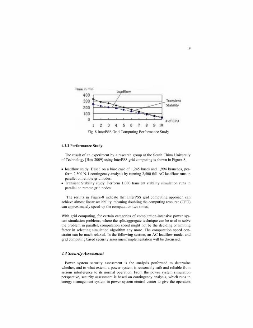
In large-scale, multi-machine power networks, it is often observed that under
certain conditions, the system might become unstable following a large distur-
bance, such as a fault, as illustrated in Figure-11. The exact reason causing the in-
stability in large-scale multi-machine power networks has not been fully unders-
tood in general, since an adequate approach to fully analyze the dynamic behavior
near the stability limit region is not available to date - at least to our knowledge.
The following three approaches are currently often used for power system stability
study:
• Time-domain simulation: Time-domain based transient stability simulation can
very accurately simulate power system dynamic behavior following a large dis-
turbance. The simulation results are displayed as a set of time-domain curves for
power engineers to examine. Some trend analysis, using for example, data-
28
mining techniques, might be performed in addition, for pattern identification.
Yet, by examining the time domain points, it is not possible to pin-point the ex-
act reason that caused the system instability.
• Small-signal stability analysis: Linear small-signal stability analysis is some-
times performed at certain operation point(s). Today, to our knowledge, analysis
in this category are performed at steady-state, pre-disturbance operation point.
Power system is non-linear, especially when it is approaching the stability limit
region. It is known that this type of linear approach, applied at pre-disturbance
operation point, in general, is not capable of predicting, with any certainty,
power system behavior in the stability limit region following a large distur-
bance.
• Transient energy function (TEF) analysis: TEF is also performed around pre-
disturbance steady-state condition. Its accuracy to predict power system dynam-
ic behavior in the stability limit region following a large disturbance has not
been proven and convinced the power engineering community.
Fig. 11 Stability Limit Region
In summary, the time-domain simulation approach is quite accurate, yet, the si-
mulation result - currently recorded as a set of time-domain points, could not be
used for in-depth power system dynamic behavior analysis. The linear small-
signal analysis approach is very powerful in terms of analysis functionality, yet, it
is currently only applied to pre-disturbance steady-state condition, which is known
to be unable to accurately predict power system dynamic behavior following a
large disturbance. A research project is currently underway at InterPSS to combine

29
these two approaches together to perform continuous small signal analysis along
the trajectory following a large disturbance, calculated using the time-domain si-
mulation approach. Similar approach has been used in voltage stability analysis,
where a load change trajectory is manually picked, and multiple loadflow calcula-
tions and Jacobian matrix analysis are performed along the load-changing trajecto-
ry to determine voltage stability.
6.2 Trajectory-based Stability Analysis
It would be interesting to systematically analyze large-scale multi-machine
power system dynamic behavior around the stability limit region, using the com-
bination of time-domain simulation and small-signal stability analysis. The differ-
ence between the trajectory-based approach and the commonly used voltage sta-
bility approach is that in the trajectory-based approach, the trajectory is accurate,
obtained by time-domain transient stability simulation, following a large distur-
bance, while in voltage stability analysis, the trajectory, obtained by increasing
load to find voltage stability limit, is somewhat artificial. In the trajectory-based
stability analysis, voltage stability analysis along the trajectory could be also per-
formed, since deteriorating voltage and reactive power conditions in the stability
limit region might be, in certain situations, the cause or a major contributing factor
to the system instability. It is our belief that the dynamic behavior analysis around
the stability limit region, obtained by time-domain simulation, following a large
disturbance can provide insight into large-scale power system stability problems,
which might be unknown to the power engineering community to date.
Fig. 12 Trajectory-based Stability Analysis

30
Grid computing is used to perform the combined analysis, as shown in Figure-
12. Power system simulation objects, capable of small-signal stability and voltage
stability analysis, are serialized along the trajectory during the time-domain tran-
sient stability simulation into XML documents and distributed over the network to
the remote slave grid nodes. Then the XML document is de-serialized at the re-
mote grid nodes into the original object model and becomes ready for small-signal
stability and voltage-stability analysis. This is still an on-going InterPSS research
project. Future research result will be posted at InterPSS Community Site [Zhou
2005].
6.3 PMU Data Processing
One situation, where the trajectory-based stability analysis approach might be
applicable in the future, is in the area of PMU (Phasor Measurement Unit) data
processing. PUM measurement data describes in real-time power system operation
states, which could be considered equivalent to the points on the trajectory de-
scribing the system dynamic behavior. The points could be sent in real-time to a
grid computing-based distributed parallel power system simulation environment to
perform small-signal stability and voltage stability analysis to evaluate system sta-
bility to identify potential risky conditions and give early warning if certain pat-
terns, which might have high rick to lead to system instability based on historic
data analysis, are identified. This approach is similar to how large investment
banks in US, such as Goldman Sachs, process the market data in real-time using
their high-performance distributed parallel computing environment to make their
investment decisions.
7. Summary
There are many challenges when attempting to adapt the existing legacy power
system simulation software packages, which were created many years ago, mostly
using FORTRAN programming language and the procedural programming ap-
proach, to the new IT environment to support the real-time software application
requirements. Among other things, the legacy power system simulation software
packages are multi-thread unsafe. The simulation state in computer memory is dif-
ficult to be distributed from one computer to another. How to architect and design
power system simulation software systems to take advantage of the latest distri-
buted IT infrastructure and make it suitable for real-time application has been dis-
cussed in this chapter, using the InterPSS software project as a concrete example.
A model-based power system software development approach has been pre-
sented. In this approach, a power system simulation object model is first created

31
and placed at the center of the development process, and the rest of the software
components evolve around the object model. Power system simulation algorithms
are implemented in a de-coupled way following the visitor software design pattern
with regard to the model so that different algorithm implementations can be ac-
commodated.
Power system software systems are very complex. They normally take many
years to evolve and become mature. Open, flexible and extensible software archi-
tecture, so that others can modify the existing functionalities and add new features,
is very important for the software evolution. The InterPSS core simulation engine
is such an example. It was first developed for a desktop application. Because of its
simplicity and open architecture, it has been late ported to a grid computing plat-
form and a cloud computing environment.
Application of InterPSS grid computing to power system security assessment
has been discussed. Accurate full AC loadflow model is used in the security as-
sessment computation. It has been shown that InterPSS grid computing approach
can achieve linear scalability. Application of InterPSS to power system stability
analysis using the trajectory-based stability analysis approach, which is currently
an on-going InterPSS research project, has been outlined.
8. Looking Beyond
All the above has been focusing on how to get the simulation or analysis results
quickly and in real-time. Naturally the next question would be, after you get all the
results, how to act on them. This is where Complex Event Processing (CEP)
[Luckham, 2002] might be playing an important role in the future. Natural events,
such as thunder storm, or human activities (events), such as switching on/off
washing machine, happen all the time. Most events are harmless, since the im-
pacted natural or man-made systems, such as power system, are robust enough to
handle and tolerate the event, and transition safely to a new steady-state. However,
there are cases that certain event or combination of events might lead to disaster.
Power system blackout is such an example, where large disturbance (event) causes
cascading system failures. In power system operation, monitoring the events and
correlating them to identify potential issues to prevent cascading system failure or
limit the impact of such failure is currently conducted by human system operator.
CEP refers using computer system to process events happening across different
layers of a complex system, identify the most meaningful event(s) within the event
cloud, analyze their impact, correlate the events, and take subsequent action(s), if
necessary, in real time. Event correlation is most interesting, since it might identi-
fy certain event pattern, which, based on historic data or human experience, might
lead to disaster. If such pattern is identified in real-time, early warning could be
sent out and immediate action taken to prevent disaster happening or limit its im-

32
pact. We believe that CEP has the potential to be used in power system control
center to assist system operator to:
• Monitor system operation and recommend preventive or corrective action based
on system operating rules when certain system situation (event) occurs;
• Correlate system events and give early warning of potential cascading failure
risk;
• Synthesis real-time on-line power system analysis information and give recom-
mendations for preventive correction to power system operation.
CEP application to power system operation will require significant effort to
modernize current power system control center IT infrastructure to be ready for
real-time IT concept and technology. In 2005, the author spent about a year at
Goldman Sachs, working with their middleware messaging IT group to support
the firm’s real-time stock trading infrastructure. The goal of stocking trading is to
maximize potential profit while controlling the risk (exposure) of the entire firm.
Power System operation has a similar goal – to optimize power generation, trans-
mission and distribution while maintaining the system reliability, stability and se-
curity margin. It is our belief that the real-time information technology, developed
in the Wall Street over the last 20 years, could be applied to power system opera-
tion to make power system a “Smart” grid in the future. To apply the real-time in-
formation technology to future power control center, we see a strong need for re-
search and development of distributed parallel power system simulation
technology using modern software development concept and methodology. The
InterPSS project is such an attempt, using modern software technology to solve a
traditional classic power engineering problem in anticipating the application of
real-time information technology and CEP to power system operation in the near
future.

33
Acknowledgement
The author would like to acknowledge the contribution to the InterPSS project
from the power system group at South China University of Technology, under the
leadership of Professor Yao Zhang, with special thanks to Professor Zhigang Wu
of South China University of Technology; Stephen Hao, currently a Ph.D. student
at Arizona State University; Tony Huang, currently a graduate student at South
China University of Technology.
Reference
Balu (1992), N., et al, “On-line Power System Security Analysis”, Proc of the
IEEE, Vol. 80, No. 2, Feb 1992.
Dean (2004), F., “MapReduce: Simplified Data Processing on Large Clusters”,
(available on the Web), 2004
Eclipse (2004), “Eclipse Modeling Framework”, http://www.eclipse.org/ model-
ing/emf/, 2010
Flower (2004), M., “Inversion of Control Containers and the Dependency Injec-
tion pattern”, (available on Web) 2004
Gamma (1994), E., et al, “Design Patterns: Elements of Reusable Object-Oriented
Software” Addison-Wesley. 1994.
Hou (2009), G., et al, “A New Power System Grid Computing Platform Based on
Internet Open Sources”, Power System Automation (Chinese), No.1, Vol 33, 2009
IEEE Task Force (1973), "Common Data Format for the Exchange of Solved
Load Flow Data", IEEE Trans on PAS, Vol. PAS-92, No. 6, Nov/Dec 1973, pp.
1916-1925.
Lin (2006), Y., et al, "Simple Application of Parallel Processing Techniques to
Power System Contingency Calculations", N American T&D Conf & Expo June
13-15, 2006, Montreal, Canada
Luckham (2002), D., “The Power of Events: An Introduction to Complex Event
Processing in Distributed Enterprise Systems”, Addison-Wesley, 2002
OMG (2001), “Model-Driven Architecture”, http://www.omg.org/mda/, 2001
OMG (2002), “Unified Modeling Language”, http://www.omg.org/ spec/UML/,
2000
SpringSource (2010), “The Spring Framework”, www.springsource .org, 2010
Stott (1974), B. et al, "Fast Decoupled Load Flow", IEEE Trans on PAS, Vol.
PAS-93(3), pp.859~869, Mar 1974
Tinney (1967), W. F., et al, "Direct Solution of Sparse Network Equation by Op-
timal Ordered Triangular Factorization", Proceeding of IEEE, Vol.55 No.11, pp
1801~1809, 1967
W3C (2010), “XML Schema”, http://www.w3.org/XML/Schema, 2010

34
Waldo (1994), J., et al, "A Note on Distributed Computing" Nov 1994 (available
on the Web)
Wood (1984) A. J., et al, "Power Generation Operation and Control", John Wiley
& Sons, Inc, 1984
Zhou (1996), E., "Object-oriented Programming, C++ and Power System Simula-
tion", IEEE Trans. on Power Systems, Vol.11, No.1, Feb. 1996 pp206-216.
Zhou (2005), M., et al, “InterPSS Community Site” http://community.interpss.org
2005