parallel and distributed systems lab. - purdue university · parallel and distributed systems lab -...

Parallel and Distributed Systems Lab - Research Overview 3/02

Parallel and Distributed Systems Lab.

Department of Computer SciencesPurdue University.

Jie Chi, Ronaldo Ferreira, Ananth Grama, Tzvetan Horozov,Ioannis Ioannidis, Mehmet Koyuturk, Shan Lei, Robert Light,

Ramakrishna Muralikrishna, Paul Ruth, Amit Shirsat

http://www.cs.purdue.edu/homes/ayg/[email protected]

____________________________________________________________

Acknowledgements: National Science Foundation, Department of Energy (Krell Fellowship),Department of Education (GAANN Fellowship).


Areas of Research:

• High Performance Computing Applications

• Large-Scale Data Handling, Compression, and Data Mining

• System Support for Parallel and Distributed Computing

• Parallel and Distributed Algorithms


High Performance Computing Applications:

• Fast Multipole Methods

• Particle Dynamics (Molecular Dynamics, Materials Simulations)

• Fast Solvers and Preconditioners for Integral Equation Formulations

• Error Control

• Preconditioning Sparse Linear Systems

• Discrete Optimization

• Visualization


Large-Scale Data Handling, Compression, and Mining:

• Bounded Distortion Compression of Particle Data

• Highly Asymmetric Compression of Multimedia Data

• Data Classification and Clustering Using Semi-Discrete

Matrix Decompositions.


System Support for Parallel and Distributed Computing:

• MOBY: A Wireless Peer-to-peer Network

• Scalable Resource Location in Service Networks

• Scheduling in Clustered Environments


Parallel and Distributed Algorithms:

• Scalable Load Balancing Techniques

• Metrics and Analysis Frameworms (Isoefficiency, Architec-

ture Abstractions for Portability)


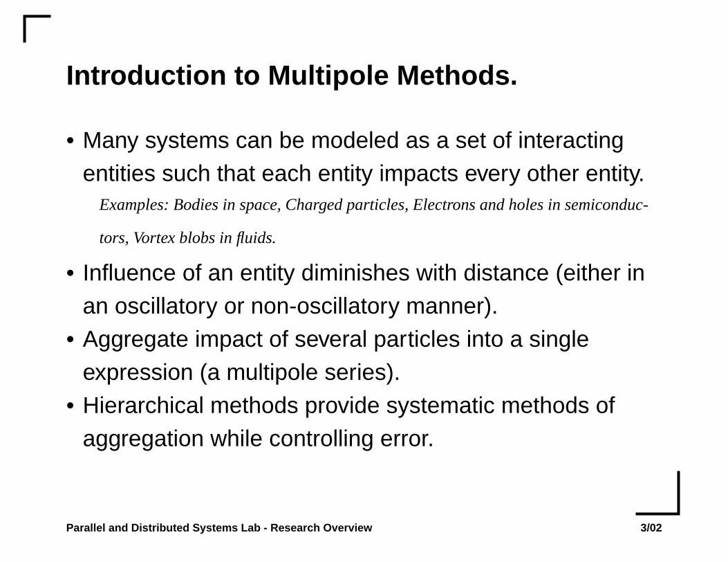
Introduction to Multipole Methods.

• Many systems can be modeled as a set of interactingentities such that each entity impacts every other entity.

Examples: Bodies in space, Charged particles, Electrons and holes in semiconduc-

tors, Vortex blobs in fluids.

• Influence of an entity diminishes with distance (either inan oscillatory or non-oscillatory manner).

• Aggregate impact of several particles into a singleexpression (a multipole series).

• Hierarchical methods provide systematic methods ofaggregation while controlling error.



• Represent the domain hierarchically using a spatial tree.

Set of particles Can they be approximated If not, divide domain andimpacting x. by their center of mass? recursively apply the same

criteria to sub-domains.

• Accurate formulation requires O(n2) force computations.• Hierarchical methods reduce this complexity to O(n) or

O(n log n).• Since particle distributions can be very irregular, the tree

can be highly unbalanced.

x x x



Fast Multipole Method (FMM)construct hierarchical representation of domain/* top down pass */for each box in tree {

construct well separated box list

for each box in well separated listtranslate multipole expansion of box and add

}for each leaf node

translate series to particle position and apply

Well separatedness criteria:

r r3 x r



• Each of the three phases, tree construction, series com-putation, and potential estimation are linear in number ofparticles n for uniform distributions.

• For non-uniform distributions, the complexity can beunbounded!

• Using box collapsing and fair-split trees, we can make thecomplexity distribution independent.



Solving Boundary Element Problems:

Boundary element methods result in a dense linearsystem:

• E(X) is the known physical quantity (boundary value),• Eo(X) is the unknown (Both are defined over the

domain ).• f(a,b) is a function of points a and b and is a decayingfunction of the distance r between a and b.

E χ( ) Eo χ( ) γ Eo χ( ) f χ X,( ) Xd

Φ∫+=

φ



Boundary Element Method for Integral Equations:

Solution of the integral form of Laplace equation:• E(X): specified boundary conditions,• Eo(X): vector of unknowns,

• The function f is the Green’s function of Laplace’sequation.

f(r) = -log (r) (in two-dimensions)f(r) = 1/r (in three-dimensions)



• Boundary integral forms are particularly suited to prob-lems where boundary conditions cannot be easily speci-fied.

• For example, while solving the field integral equations

(EFIE/MFIE/CFIE), the associated Green’s function (eikr/

r) implicitly satisfies boundary conditions at infinity. Thisobviates the need for absorbing boundary conditions.

• Surface integral equations are, however, infeasible fornon-homogeneous media, consequently, a mixed finiteelement / boundary element approach is often used.


Experimental Results:

Sample charge distribution.


Experimental Results:

Force vectors at charges.


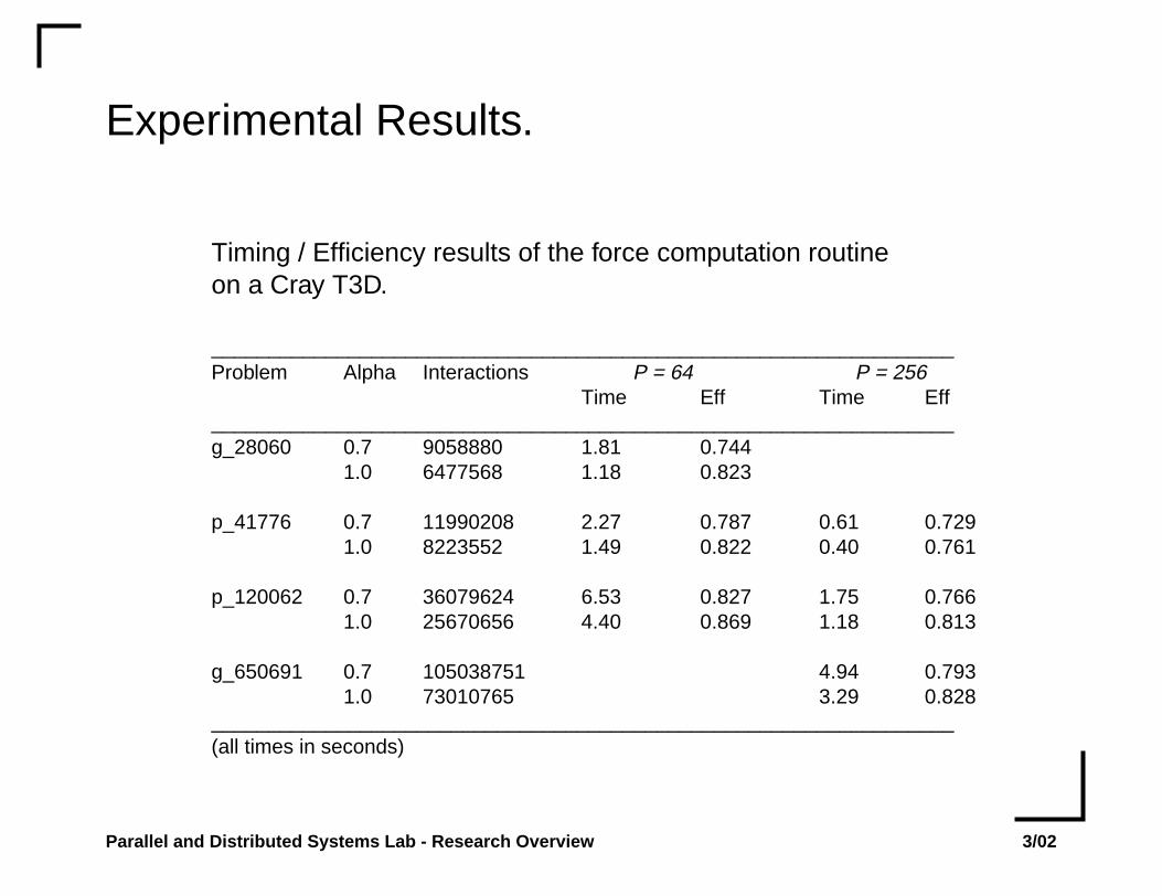
Experimental Results.

Timing / Efficiency results of the force computation routineon a Cray T3D.

_________________________________________________________________Problem Alpha Interactions P = 64 P = 256

Time Eff Time Eff_________________________________________________________________g_28060 0.7 9058880 1.81 0.744

1.0 6477568 1.18 0.823

p_41776 0.7 11990208 2.27 0.787 0.61 0.7291.0 8223552 1.49 0.822 0.40 0.761

p_120062 0.7 36079624 6.53 0.827 1.75 0.7661.0 25670656 4.40 0.869 1.18 0.813

g_650691 0.7 105038751 4.94 0.7931.0 73010765 3.29 0.828

_________________________________________________________________(all times in seconds)


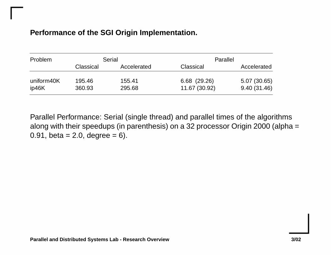
Performance of the SGI Origin Implementation.

Problem Serial ParallelClassical Accelerated Classical Accelerated

uniform40K 195.46 155.41 6.68 (29.26) 5.07 (30.65)ip46K 360.93 295.68 11.67 (30.92) 9.40 (31.46)

Parallel Performance: Serial (single thread) and parallel times of the algorithmsalong with their speedups (in parenthesis) on a 32 processor Origin 2000 (alpha =0.91, beta = 2.0, degree = 6).


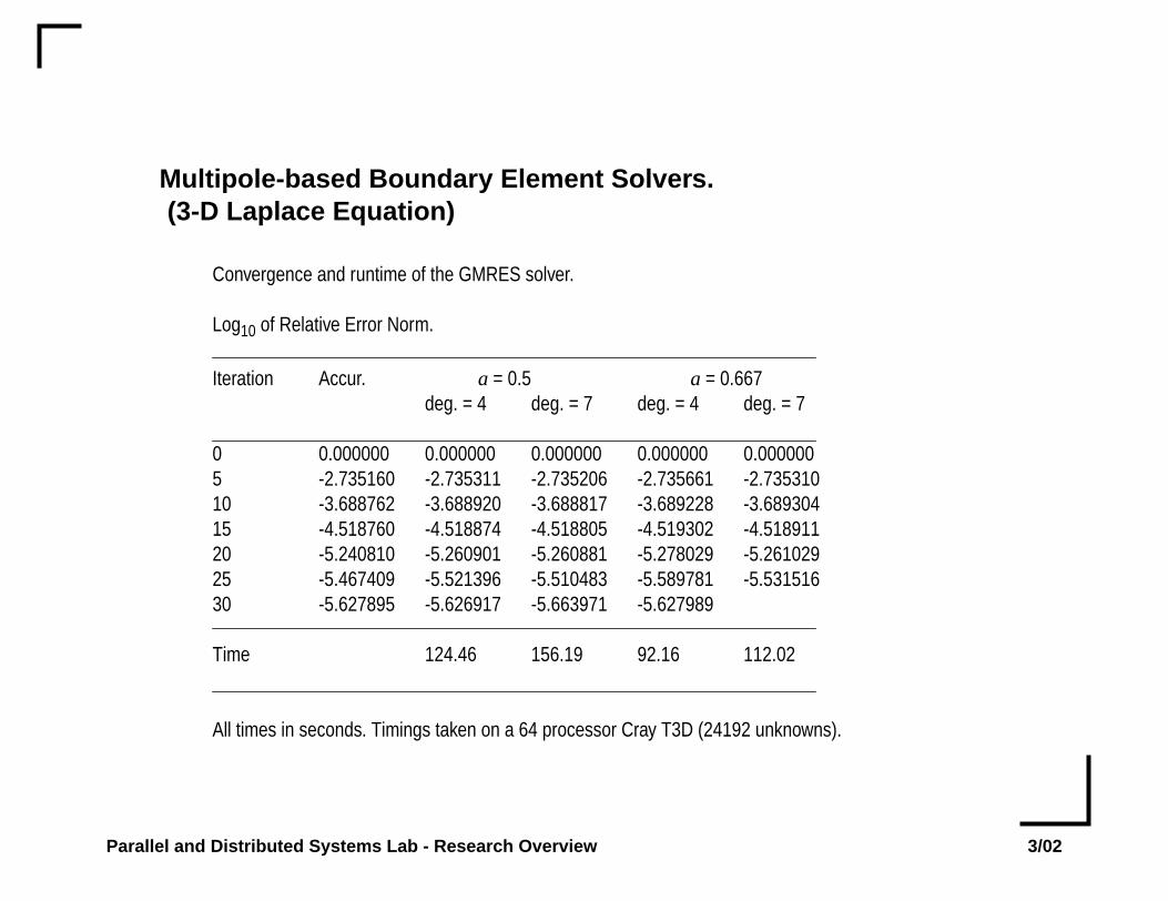
Multipole-based Boundary Element Solvers.(3-D Laplace Equation)

Convergence and runtime of the GMRES solver.

Log10 of Relative Error Norm.

Iteration Accur. a = 0.5 a = 0.667deg. = 4 deg. = 7 deg. = 4 deg. = 7

0 0.000000 0.000000 0.000000 0.000000 0.0000005 -2.735160 -2.735311 -2.735206 -2.735661 -2.73531010 -3.688762 -3.688920 -3.688817 -3.689228 -3.68930415 -4.518760 -4.518874 -4.518805 -4.519302 -4.51891120 -5.240810 -5.260901 -5.260881 -5.278029 -5.26102925 -5.467409 -5.521396 -5.510483 -5.589781 -5.53151630 -5.627895 -5.626917 -5.663971 -5.627989

Time 124.46 156.19 92.16 112.02

All times in seconds. Timings taken on a 64 processor Cray T3D (24192 unknowns).


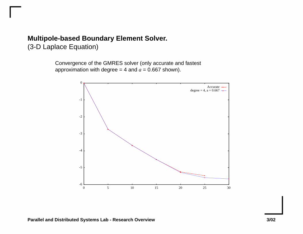
Multipole-based Boundary Element Solver.(3-D Laplace Equation)

Convergence of the GMRES solver (only accurate and fastestapproximation with degree = 4 and a = 0.667 shown).

-6

-5

-4

-3

-2

-1

0

0 5 10 15 20 25 30

Accuratedegree = 4, a = 0.667

Iterations

RelativeErrorNorm


Multipole-based Boundary Element Solver.(3-D Laplace Equation)

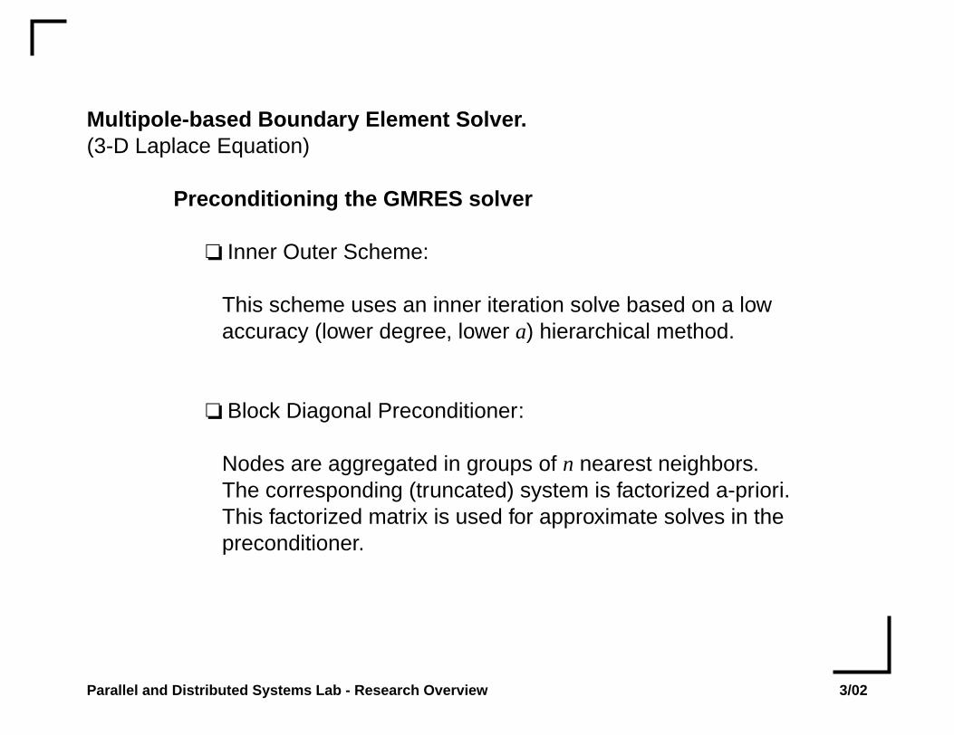
Preconditioning the GMRES solver

❏ Inner Outer Scheme:

This scheme uses an inner iteration solve based on a lowaccuracy (lower degree, lower a) hierarchical method.

❏ Block Diagonal Preconditioner:

Nodes are aggregated in groups of n nearest neighbors.The corresponding (truncated) system is factorized a-priori.This factorized matrix is used for approximate solves in thepreconditioner.


Multipole-based Boundary Solvers.(3-D Laplace Equation)

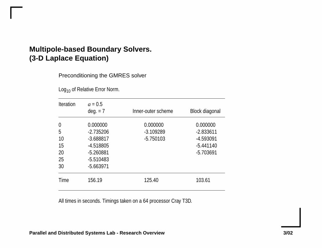
Preconditioning the GMRES solver

Log10 of Relative Error Norm.

Iteration a = 0.5deg. = 7 Inner-outer scheme Block diagonal

0 0.000000 0.000000 0.0000005 -2.735206 -3.109289 -2.83361110 -3.688817 -5.750103 -4.59309115 -4.518805 -5.44114020 -5.260881 -5.70369125 -5.51048330 -5.663971

Time 156.19 125.40 103.61

All times in seconds. Timings taken on a 64 processor Cray T3D.


Using Multipole Methods for PreconditioningSparse Iterative Solvers.

Problem Formulation

❏ Arises in simulation of time-dependent Navier-Stokesequations for incompressible fluid flow

❏ One of the most time consuming steps

❏ Large scale 3D domains

❏ Multiprocessing is indispensable

❏ Robust, parallel preconditioners required


Nature of the System and Preconditioning.

Linear System

where

, in which and

M : Mass matrix; T : Laplace operator B : Gradient operator (n x k)

Properties of the Linear System

Symmetric indefinite (n +ve and k -ve eigenvalues)

Typically (2D) or (3D)

A B

BT 0

up

f0

=

A αM νT+= α 1∆t-----≅ ν 1

Re------≅

kn8---= k

n24------=


Uzawa-type Methods

Solve using iterative method

Accelerate by CG

Assumption : div-stability is well-conditioned1 (steady state)

Single-level iterative schemes with suitable preconditioning

Key Issues

Two-level nested iteratitve schemes

Expensive iterations due to inner iterative solver

1. Condition number independent of mesh discretization

BT A1–Bp BT A

1–f=

B⇒ TA1–B


Adapting Dense Methods to the PreconditioningProblem

Use a dense solver to compute the preconditioner forthe matrix A.

The dominant behavior of matrix A is .

The Green’s function of this operator is .

Issue: Implementing boundary conditions?

∇∇ k2

–( )

ekr–

r------------


Implementing Boundary Conditions for DensePreconditioner

Analogous problem in potential theory: Compute the potential over a domainresulting from a set of given charges provided the boundary potential is pre-specified.

Solution strategy:

Assume (unknown) charges residing on the boundary.

The result of the boundary and internal charges result in the boundary condi-tions. Use this to compute the values of the unknown boundary charges.

Finally, use these boundary charges along with given internal charges tocompute the potential in the interior.

Computational steps: a dense boundary element solve of an n x n system (forn boundary nodes) followed by a dense mat-vec with an n x n system.


Preconditioning Effect of Dense Solvers:

Preconditioning of Hierarchical Approximate Techniques

IncompleteFactorization

HierarchicalApproximation

297 14 9

653 20 14

1213 25 14

2573 35 16

4953 45 18

ni


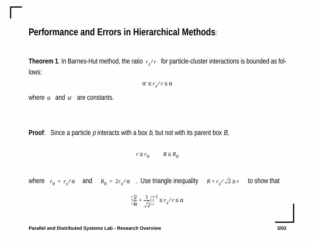
Performance and Errors in Hierarchical Methods :

Theorem 1 . In Barnes-Hut method, the ratio for particle-cluster interactions is bounded as fol-

lows:

where and are constants.

Proof : Since a particle p interacts with a box b, but not with its parent box B,

where and . Use triangle inequality to show that

r s r⁄

α' r s r⁄ α≤ ≤

α α'

r r 0≥ R R0≤

r0 r s α⁄= R0 2r s α⁄= R rs 2⁄+ r≥

2α--- 1

2-------+

1–r s r⁄ α≤ ≤


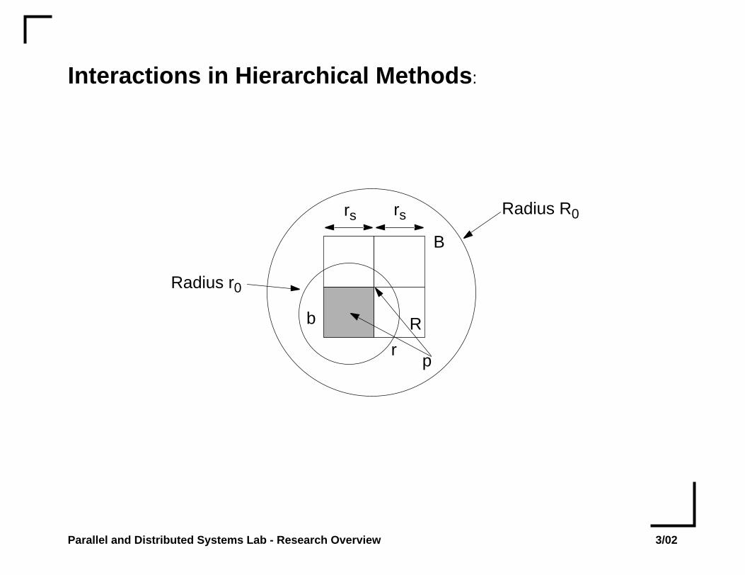
Interactions in Hierarchical Methods :

B

b

pr

R

rs rs Radius R0

Radius r0


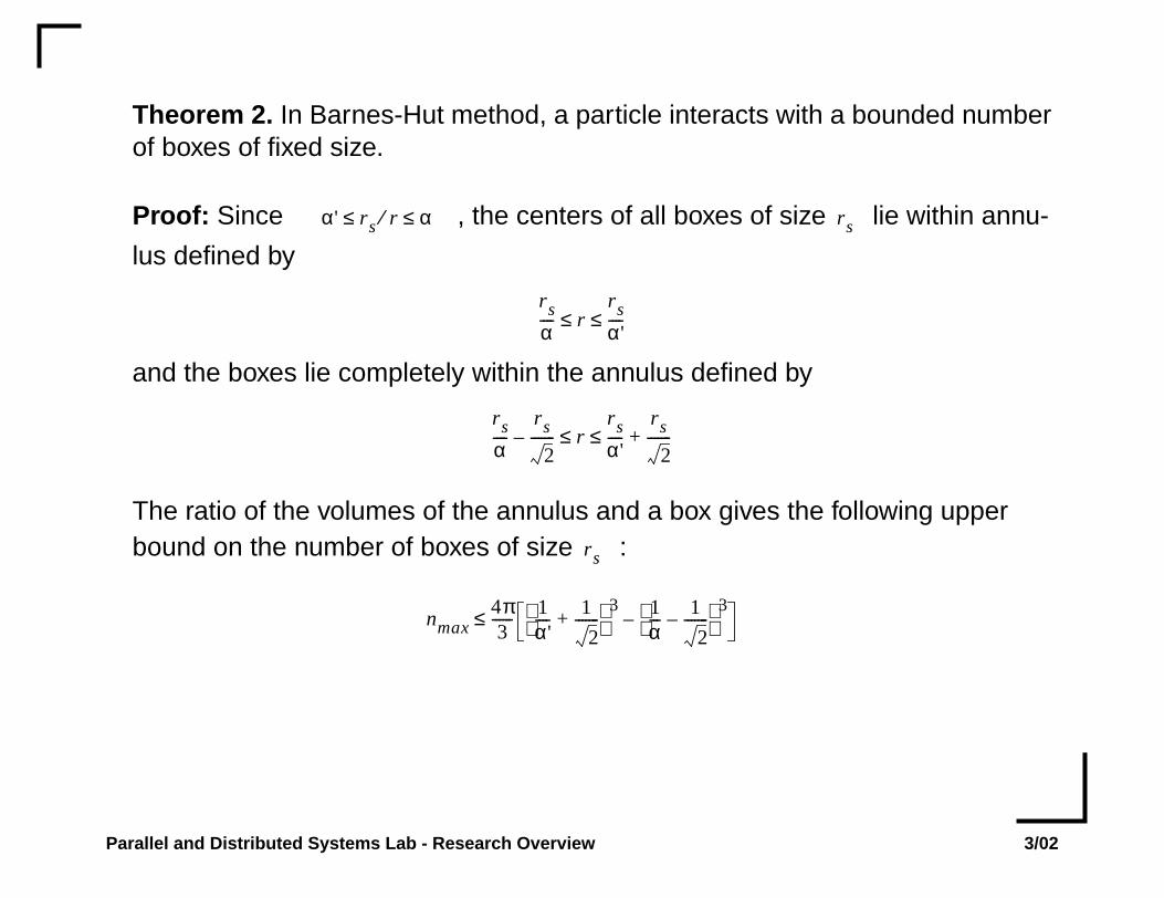
Theorem 2. In Barnes-Hut method, a particle interacts with a bounded numberof boxes of fixed size.

Proof: Since , the centers of all boxes of size lie within annu-

lus defined by

and the boxes lie completely within the annulus defined by

The ratio of the volumes of the annulus and a box gives the following upperbound on the number of boxes of size :

α' r s r⁄ α≤ ≤ r s

rs

α---- r

r s

α'----≤ ≤

r s

α----

r s

2-------– r

r s

α'----

r s

2-------+≤ ≤

r s

nmax4π3

------ 1α'---- 1

2-------+

3 1α--- 1

2-------–

3–≤


Theorem 3. Suppose that k charges of strengths { , j=1,...,k} are located

within a sphere of radius . Then, for Barnes-Hut method with -criterion for

well-separatedness, the error in potential outside the sphere at a distancefrom the center of the sphere due to these charges is bounded by

where p is the degree of the truncated multipole expansion such that , and

qj

rs α

r

ε Ar r s–-------------

r s

r----

p 1+ A

rs---- αp 2+

1 α–---------------⋅≤⋅≤

p 1>

A qjj 1=

k

∑=


Theorem 4 . Controlling error in B-H

The theorem defines a growth rate for the polynomial degree with the netcharge inside a subdomain such that the total error associated with the subdo-main remains constant.

For a uniform distribution, this growth rate can also be expressed in terms of thedomain sizes.

pk pkd

αlog------------

Alog Aklog–

αlog---------------------------------+ +=


Theorem 5 . Error in the piecewise approximate B-H method

This follows naturally from the following results:

- The number of interactions with subdomains at any level are constant.

- The number of subdomain interactions is logarithmic in number of particles(independent of particle distribution -- sequence of theorems on fair-splittrees omitted).

- The error associated with a single particle-subdomain interaction is con-stant.

O αp 1+ Alog( )


Theorem 6 . Computational complexity of the piecewise approximate B-Hmethod

where l is the levels of the hierarchical decomposition.

For a uniform distribution, l grows as log8n.

For l < p, we can show that the operation count of the new method is within afraction 7/3 of the fixed-degree multipole method. For smaller values of l this dif-ference is smaller.

For typical values of p (6 - 7 degree approximations), this corresponds tobetween 256K - 2M node points. Thus, even for very large scale simulations,the improved method is within a small constant off the fixed-degree methodwhile yielding significant improvements in error.

O n p l+( )3( )


Comparison of Errors


Comparison of Runtimes


Bounded Error Pointset Compression Results

2568 10K 20K 100K0

2

4

6

8

10

12

14

Number of Particles

Com

pres

sion

Rat

io

Compression Ratio of Various Schemes

UncompressedGzipped Scheme1 Scheme2 Scheme3 Scheme4


Some Other Parallel Applications: Shear-Warp.shear

project

warp


Optimizations for volume Rendering:

Early Termination:

Instead of traveling back to front, it is possible to travelfront to back. In this case, it is possible to stop when theaccrued opacity is high enough that additional slices donot make any difference.

Skipping Empty Spaces:

In typical datasets, a significant part of the volume is empty(the opacity is 0). These voxels need not be traversed. Usingsmart data-structures, it is possible to skip these all-together.Run-length encode the scanlines.


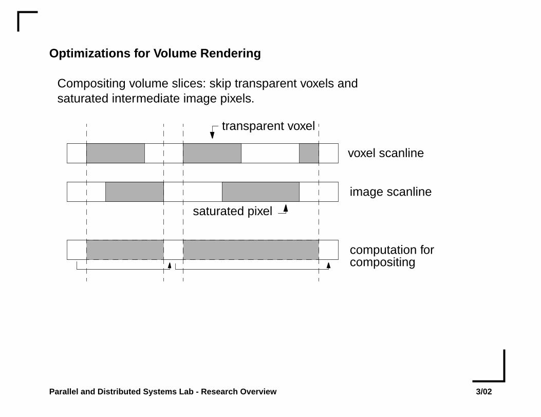
Optimizations for Volume Rendering

Compositing volume slices: skip transparent voxels andsaturated intermediate image pixels.

transparent voxel

voxel scanline

saturated pixel

image scanline

computation forcompositing


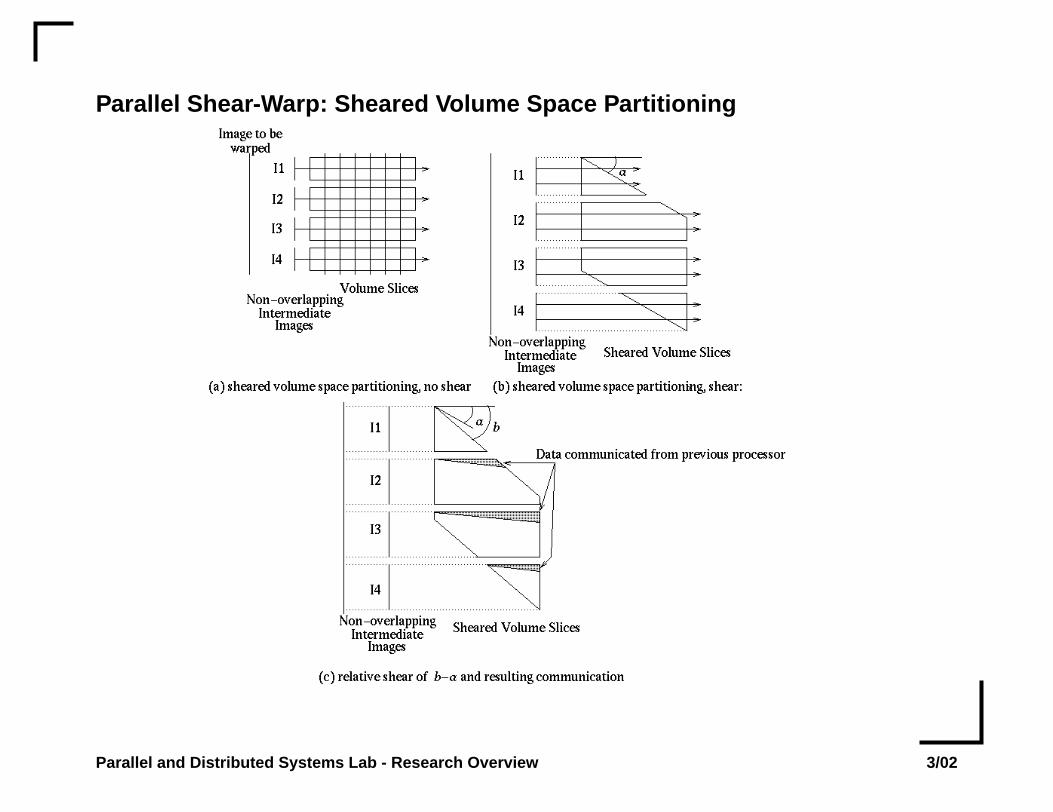
Parallel Shear-Warp: Volume Space Partitioning


Parallel Shear-Warp: Sheared Volume Space Partitioning


Load Balancing

❏ Due to optimizations such as run-length encoding andearly termination, different scanlines can have widelyvarying workloads.

❏ Naively partitioning the sheared volume among processorsleads to significant load imbalance.

❏ It is impossible to determine the load associated with ascanline accurately a-priori.

❏ Since the viewpoint is not expected to shift very drasticallybetween frames, we can use load information from one frameto balance load in the next.

❏ Each processor keeps track of load at each scanline. At theend of computation, processors exchange this information andrebalance load. The communication can be integrated with shear.


Experimental Results (the brain dataset)


Rendering Time (ms)

p volumeNo load balance Load BalancedLarge Small Large Small

1 3193 976 3193 9762 1627 548 1625 5514 892 309 910 3108 620 197 593 19616 345 127 327 12132 216 86 204 8164 142 74 118 70128 103 85


Large-Scale Data Handling, Compression, and Mining.

Proximus: a tool for bounded error compression of discrete attrubute sets.


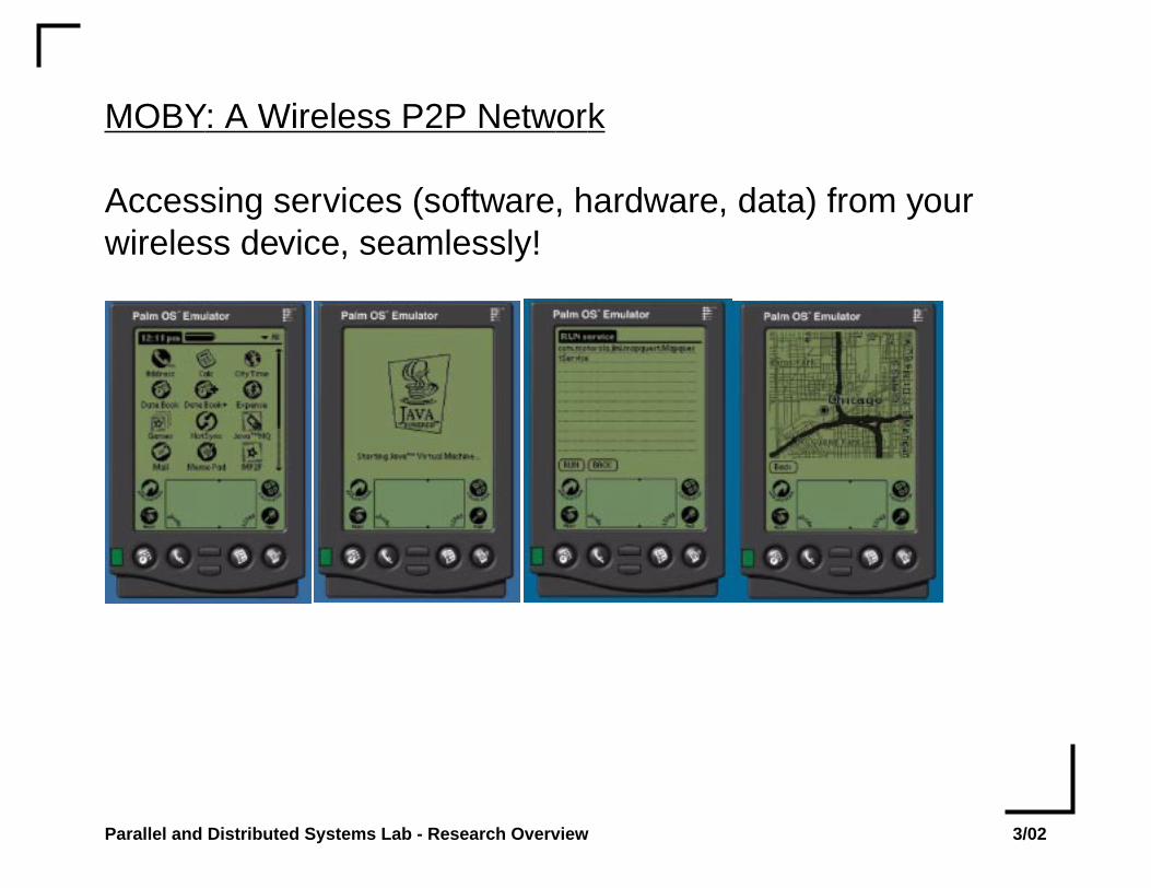
MOBY: A Wireless P2P Network

Accessing services (software, hardware, data) from yourwireless device, seamlessly!


Other Research on P2P Networks:

Evolving Topology Based on Access Patterns

Service Mobility

Dynamic Client Mapping.

parallel and distributed systems lab. - purdue university · parallel and distributed systems lab -...

Documents