dissertation third-generation site characterization

DISSERTATION

THIRD-GENERATION SITE CHARACTERIZATION: CRYOGENIC CORE COLLECTION,

NUCLEAR MAGNETIC RESONANCE, AND ELECTRICAL RESISTIVITY

Submitted by

Saeed Kiaalhosseini

Department of Civil and Environmental Engineering

In partial fulfillment of the requirements

For the Degree of Doctor of Philosophy

Colorado State University

Fort Collins, Colorado

Fall 2016

Doctoral Committee:

Advisor: Thomas Sale Co-Advisor: Jens Blotevogel Richard Johnson Gregory Butters

Copyright by Saeed Kiaalhosseini 2016

All Rights Reserved

ii

ABSTRACT

THIRD-GENERATION SITE CHARACTERIZATION: CRYOGENIC CORE COLLECTION,

NUCLEAR MAGNETIC RESONANCE, AND ELECTRICAL RESISTIVITY

In modern contaminant hydrology, management of contaminated sites requires a holistic

characterization of subsurface conditions. Delineation of contaminant distribution in all phases

(i.e., aqueous, non-aqueous liquid, sorbed, and gas), as well as associated biogeochemical

processes in a complex heterogeneous subsurface, is central to selecting effective remedies.

Arguably, a factor contributing to the lack of success of managing contaminated sites effectively has

been the limitations of site characterization methods that rely on monitoring wells and grab

sediment samples. The overarching objective of this research is to advance a set of third-

generation (3G) site characterization methods to overcome shortcomings of current site

characterization techniques. 3G methods include 1) cryogenic core collection (C3) from

unconsolidated geological subsurface to improve recovery of sediments and preserving key

attributes, 2) high-throughput analysis (HTA) of frozen core in the laboratory to provide high-

resolution, depth discrete data of subsurface conditions and processes, 3) resolution of non-

aqueous phase liquid (NAPL) distribution within the porous media using a nuclear magnetic

resonance (NMR) method, and 4) application of a complex resistivity method to track NAPL

depletion in shallow geological formation over time.

A series of controlled experiments were conducted to develop the C3 tools and methods.

The critical aspects of C3 are downhole circulation of liquid nitrogen via a cooling system, the

strategic use of thermal insulation to focus cooling into the core, and the use of back pressure to

iii

optimize cooling. The C3 methods were applied at two contaminated sites: 1) F.E. Warren

(FEW) Air Force Base near Cheyenne, WY and 2) a former refinery in the western U.S. The

results indicated that the rate of core collection using the C3 methods is on the order of 30

foot/day. The C3 methods also improve core recovery and limits potential biases associated with

flowing sands.

HTA of frozen core was employed at the former refinery and FEW. Porosity and fluid

saturations (i.e., aqueous, non-aqueous liquid, and gas) from the former refinery indicate that

given in situ freezing, the results are not biased by drainage of pore fluids from the core during

sample collection. At FEW, a comparison between the results of HTA of the frozen core

collected in 2014 and the results of site characterization using unfrozen core, (second-generation

(2G) methods) at the same locations (performed in 2010) indicate consistently higher

contaminant concentrations using C3. Many factors contribute to the higher quantification of

contaminant concentrations using C3. The most significant factor is the preservation of the

sediment attributes, in particular, pore fluids and volatile organic compounds (VOCs) in

comparison to the unfrozen conventional sediment core.

The NMR study was performed on laboratory-fabricated sediment core to resolve NAPL

distribution within the porous media qualitatively and quantitatively. The fabricated core

consisted of Colorado silica sand saturated with deionized water and trichloroethylene (TCE).

The cores were scanned with a BRUKER small-animal scanner (2.3 Tesla, 100 MHz) at 20 °C

and while the core was frozen at -25 °C. The acquired images indicated that freezing the water

within the core suppressed the NMR signals of water-bound hydrogen. The hydrogen associated

with TCE was still detectable since the TCE was in its liquid state (melting point of TCE is -73

°C). Therefore, qualitative detection of TCE within the sediment core was performed via the

iv

NMR scanning by freezing the water. A one-dimensional NMR scanning method was used for

quantification of TCE mass distribution within the frozen core. However, the results indicated

inconsistency in estimating the total TCE mass within the porous media.

Downhole NMR logging was performed at the former refinery in the western U.S. to

detect NAPL and to discriminate NAPL from water in the formation. The results indicated that

detection of NMR signals to discriminate NAPL from water is compromised by the noise

stemming from the active facilities and/or power lines passing over the site.

A laboratory experiment was performed to evaluate the electrical response of

unconsolidated porous media through time (30 days) while NAPL was being depleted. Sand

columns (Colorado silica sand) contaminated with methyl tert-butyl ether (MTBE, a light non-

aqueous phase liquid (LNAPL)) were studied. A multilevel electrode system was used to

measure electrical resistivity of impacted sand by imposing alternative current. The trend of

reduction in resistivity through the depth of columns over time followed depletion of LNAPL by

volatilization.

Finally, a field experiment was performed at the former refinery in the western U.S. to

track natural losses of LNAPL over time. Multilevel systems consisting of water samplers,

thermocouples, and electrodes were installed at a clean zone (background zone) and an LNAPL-

impacted zone. In situ measurements of complex resistivity and temperature were taken and

water sampling was performed for each depth (from 3 to 14 feet below the ground surface at

one-foot spacing) within almost a year. At both locations, the results indicated decreases in

apparent resistivity below the water table over time. This trend was supported by the

geochemistry of the pore fluids. Overall, results indicate that application of the electrical

v

resistivity method to track LNAPL depletion at field sites is difficult due to multiple conflicting

factors affecting the geoelectrical response of LNAPL-impacted zones over time.

vi

ACKNOWLEDGMENTS

I would like to thank my advisor, professor Tom Sale, for providing me with this great

opportunity to pursue my Ph.D. at Colorado State University (CSU), Fort Collins, CO. His

knowledge and deep understanding in the field of contaminant hydrology were greatly influential

and helpful for me to conduct my Ph.D. research over the last five years. Without his

comprehensive support and encouragement, I would have not been able to finish this journey. I

would also like to thank my co-advisor, Dr. Jens Blotevogel, who provided continuous support

and guidance during development of my research. I would like to thank my committee

members, Drs. Rick Johnson and Greg Butters, for their valuable feedback and insightful

comments. Moreover, I would like to thank Dr. Chuck Shackelford who was very influential in

my education at CSU.

My friends and colleagues at the Center for Contaminant Hydrology (CCH) at CSU have

all been very supportive and kind to me over the last few years. I would like to thank Maria

Irianni Renno, Gary Dick, Mitch Olson, Helen Dungan, Jeramy Jasmann, Kevin Saller, Daria

Akhbari, Mark Chalfant, Emily Stockwell, Eric Emerson, Zoe Bezold, Rachael McSpadden,

Melissa Tracy, Molly McLaughlin, Abdulaziz Alqahtani, Anna Skinner, Jennifer Wahlberg,

Christina Ankrom, Wes Tulli, Gabrielle Davis, Hanna Smith, and Nolan Platt for their help,

support, and friendship. I would also like to thank Bart Rust and Junior Garza from the

Engineering Research Center Machine Shop at CSU.

Drs. Beth Parker and John Cherry have also provided me with the opportunity of visiting

the Center for Applied Ground Water Research Group (G360) at the University of Guelph, for

which I am very grateful. I would also like to thank Jonathan Munn, Drs. Colby Steelman,

vii

Patrick Quinn, Peter Pehme, Emmanuelle Arnaud, Jessica Meyer, Carla Rose, Carlos Maldaner,

Linda Moore, Paul Beck, Ash Stanton, Maria Gorecka, and Cinthuja Leon, and all friends who

shared their time and knowledge with me.

Without years of funding and support from the U.S. Department of Defense, Strategic

Environmental Research and Development Program, the work presented in Chapters 2 and 3 of

this dissertation would have not been possible. Also, I would like to thank Rick Rogers (Drilling

Engineers Inc.) for sharing his valuable thoughts and ideas that greatly influenced the work

presented in Chapter 2. The work in Chapter 4 was supported by General Electric funding. I

would like to thank Dr. Ted Watson and Benjamin Kohen at the Rocky Mountain Magnetic

Resonance Imaging (RMMRC) at CSU who provided precious advice and guidance to

implement this chapter. Chapter 5 was supported by the research gift fund to CSU. To

implement the research presented in this chapter, many people from TriHydro, namely, Alysha

Hakala, Thomas Gardner, Stephanie Whitfield, and Shawn Harshman supported me. I would

like to thank them all as well as Mark Lyverse from Chevron Corporation for his useful advice

and support throughout this part of the work.

I would like to thank my friends in Fort Collins, especially, Ramin Zahedi, Mehrdad

Memari, Mona Mirsiaghi, Saleh Taghvaeian, Khatoon Abrishami, Masih Akhbari, Shadi

Khademi, Mehdi Fazel, Pooria Pakrooh and all other friends who have been there for my wife

and I over the last years. I would also like to thank my parents who have always supported and

respected my decisions throughout my life and have always been there for me through thick and

thin. Last but not least, I would like to thank my wife, Azadeh, for her continuous and

unconditional love and support throughout the completion of this program and dedicate this

dissertation to her as a notion of my appreciation and gratitude towards her kindness and support.

viii

TABLE OF CONTENTS

ABSTRACT .................................................................................................................................... ii

ACKNOWLEDGMENTS ............................................................................................................. vi

TABLE OF CONTENTS ............................................................................................................. viii

CHAPTER 1 INTRODUCTION ................................................................................................... 1

1.1. Problem Statement .............................................................................................................. 1

1.2. Background ......................................................................................................................... 2

1.3. Research Objective and Hypothesis .................................................................................... 8

1.4. Publication Status ................................................................................................................ 9

CHAPTER 2 CRYOGENIC CORE COLLECTION FROM UNCONSOLIDATED

SUBSURFACE MEDIA ............................................................................................................... 11

2.1. Chapter Synopsis ............................................................................................................... 11

2.2. Introduction ....................................................................................................................... 11

2.3. Research Objective and Hypothesis .................................................................................. 15

2.4. Methods ............................................................................................................................. 15

2.4.1. C3 Tools and Operational Procedures ...................................................................... 16

2.4.2. Controlled Experiments of Freezing Time .............................................................. 20

2.4.3. Application of the C3 Method at Field Sites ............................................................ 21

2.4.4. Core Analysis .......................................................................................................... 22

2.5. Results and Discussion ...................................................................................................... 24

ix

2.5.1. Rate of Cooling Experiments .................................................................................. 24

2.5.2. Core Production and Recovery ................................................................................ 25

2.5.3. Core Analysis .......................................................................................................... 27

2.6. Summary and Conclusions ................................................................................................ 30

CHAPTER 3 CRYOGENIC CORE COLLECTION AND HIGH-THROUGHPUT ANALYSIS

OF FROZEN CORE ..................................................................................................................... 31


3.2. Introduction ....................................................................................................................... 32


3.4. Methods ............................................................................................................................. 35

3.4.1. 3G Methods ............................................................................................................. 36


3.5.1. 3G Results ................................................................................................................ 48

3.5.2. Comparison of 2G and 3G Methods at FEW .......................................................... 58


CHAPTER 4 SPATIAL DISTRIBUTION ANALYSIS OF NON-AQUEOUS PHASE

LIQUIDS IN POROUS MEDIA USING NUCLEAR MAGNETIC RESONANCE:

LABORATORY AND FIELD STUDIES .................................................................................... 62


4.2. Introduction ....................................................................................................................... 63

4.2.1. Theory of Nuclear Magnetic Resonance ................................................................. 64

x

4.2.2. Literature Review .................................................................................................... 73


4.4. Methods ............................................................................................................................. 76

4.4.1. Laboratory Study ..................................................................................................... 76

4.4.2. Field Study ............................................................................................................... 81


4.5.1. Laboratory Study ..................................................................................................... 85

4.5.2. Field Study ............................................................................................................... 90


CHAPTER 5 MONITORING DEPLETION OF LIGHT NON-AQUEOUS PHASE LIQUID IN

SHALLOW GEOLOGICAL FORMATIONS USING ELECTRICAL RESISTIVITY ............. 97


5.2. Introduction ....................................................................................................................... 98

5.2.1. Electrical Resistivity Method .................................................................................. 98

5.2.2. Literature Review .................................................................................................. 105

5.3. Research Objective and Hypothesis ................................................................................ 112

5.4. Methods ........................................................................................................................... 112

5.4.1. Laboratory Study ................................................................................................... 112

5.4.2. Field Study ............................................................................................................. 115

5.5. Results and Discussion .................................................................................................... 119

xi

5.5.1. Laboratory Study ................................................................................................... 120

5.5.2. Field Study ............................................................................................................. 121

5.6. Summary and Conclusions .............................................................................................. 130

CHAPTER 6 SUMMARY, RECOMMENDATION, AND CONCLUSION ........................... 133

Results from Chapter 2 ............................................................................................................... 133




Implications................................................................................................................................. 144

REFERENCES ........................................................................................................................... 145

APPENDIX A ............................................................................................................................. 158

APPENDIX B ............................................................................................................................. 162

APPENDIX C ............................................................................................................................. 169

APPENDIX D ............................................................................................................................. 174

1

CHAPTER 1

INTRODUCTION

The following section provides an introduction to this Ph.D. dissertation. Contents

include a problem statement, background information, research objectives, research hypotheses,

and the status of related publications.

1.1. Problem Statement

Over the last century, releases of anthropogenic chemicals into the subsurface have

resulted in widespread contamination of soils and groundwater (Stroo and Ward 2010).

Worldwide efforts to restore impacted media, at best, have been partially successful (NRC 2013).

Arguably, a factor contributing to the lack of success is an insufficient understanding of

contaminant distribution in all phases (i.e., aqueous, non-aqueous liquid, sorbed, and gas) in the

subsurface (Sale et al., 2013). Given the distinction of source zones and plumes (NRC 2005),

contaminant concentrations need to be resolved in 14 compartments as illustrated in Figure 1.1

(Sale et al., 2011). Moreover, resolution of biogeochemical conditions in each of the 14

compartments is critical to understanding natural losses of contaminants as well as the efficacy

of active remedial measures.

To date, the most common tools for site characterization have been conventional

monitoring wells and grab sediment samples, referred to herein as ″first-generation (1G)″

methods. Monitoring wells can be used to acquire information regarding aqueous phase (i.e.,

water) and continuous non-aqueous phase liquid (NAPL) in transmissive zones. However,

monitoring wells fail to resolve contaminant concentrations in sorbed and gas phases in

transmissive zones and all contaminant phases (i.e., vapor, aqueous, non-aqueous liquid, and

2

sorbed) in low-permeable (low-k) zones. Grab sediment sampling methods (e.g., hollow-stem

auger, direct push method, etc.) are also limited in many aspects, including preservation of pore

structure, pore fluids, volatile compounds, redox conditions, mineralogy, and microbial ecology

(Sale et al., 2015; Kiaalhosseini et al., 2015; Kiaalhosseini et al., 2016).

Figure 1.1. The 14 compartment model. Arrows show mass potential transfer links between compartments. Dashed arrows indicate irreversible fluxes (Sale et al., 2011).

Subsequently, second-generation (2G) site characterization techniques, that rely on the

small-scale spatial discretization of data versus depth, are a major improvement over 1G

methods. 2G methods include: 1) Membrane Interface Probe (MIP), 2) Waterloo ProfilerTM, 3)

high-resolution subsampling from continuous sediment core and analysis in the laboratory, and

4) multilevel sampling system. Given the site-specific limitations of 2G methods, they are best

applied in combination with the hope that one of the methods will prove to be effective. The

potential need to employ multiple 2G methods can lead to high costs (Sale et al., 2015).

1.2. Background

Following Sale and Johnson (2012), depiction of subsurface conditions is commonly

advanced using plan view contour maps of contaminant concentrations. Figure 1.2 shows an

example of a plan view contour map of the contaminant at F.E. Warren Airforce Base near

Cheyenne, WY. These types of maps were generated based on the analysis of water samples

3

collected from monitoring wells (1G methods). Typically, plume maps show homogeneous

bodies in the area of the contaminated site with contours grading concentrations through multiple

orders of magnitude over distances of 100s to 1000s of meters. The plume maps suggest that the

vertical distribution of contaminants is uniform through the depth.

Figure 1.2. An example of plume contour map representing contaminant concentrations at F.E. Warren Air Force Base near Cheyenne, WY (Sale and Johnson 2012).

Natural subsurface bodies often contain permeability variation spanning 3-6 orders of

magnitude. This fact creates transmissive zones where advective transport of fluids dominates

and low-k zones where diffusive transport process dominates. Water sampling from monitoring

wells fails to recognize contaminants in low-k zones. Plume contour maps represent

contaminant concentrations of aqueous and continuous NAPL from the transmissive zone and

are limited to recognizing all contaminant phases (i.e., aqueous, NAPL, sorbed, and gas) in the

subsurface. Table 1.1 summarizes the limitations of 1G methods.

4

Table 1.1. Potential limitations of 1G characterization methods (Sale et al., 2013 and 2015)

The limitations of 1G site characterization strategies led to the development of

characterization methods that focus on the collection of high-resolution, vertical data to depict

the contaminant distributions within the transmissive and low-k zones. As an example, Figure

1.3 shows a plume map generated from high-resolution data collected using multilevel sampling

systems at a contaminated site in Ontario, Canada (Guilbeault et al., 2005).

The 2G site characterization methods include:

Membrane Interface Probe (MIP)

Waterloo ProfilerTM

high-resolution subsampling from continuous sediment core and analysis in the

laboratory

multilevel sampling systems

1G Tools Limitations Monitoring wells

- In-well mixing of water from different depths obfuscates plume structure - Not effective for identification of impacted low-k zones - Leads to an incorrect conceptual model (i.e., large-and-dilute plumes, rather than structured plumes, only captures water samples from transmissive zones)

Grab sediment samples

- Loss of volatile compounds - Loss of sediment structure - Drainage of pore fluids

5

Figure 1.3. Results of a tetrachloroethylene (PCE) contaminated site at Ontario, Canada using 2G methods a) PCE distribution projected onto the cross section of the site b) major profiles of PCE concentrations versus depth (Guilbeault et al., 2005).

2G tools revealed the previously-missed perspective of subsurface contaminant occurrence

including:

the existence of contaminants that have diffused into the low-k zones

diffusion/sorption controlled transport of contaminants within the low-k zones

Although 2G strategies progress the understanding of subsurface contaminant conditions,

Sale et al. (2013) discussed the limitations of 2G methods. The limitations of 2G site

characterization are summarized in Table 1.2.

Limitations of 1G and 2G methods motivated efforts in this study to advance a set of new

″third-generation (3G)″ methods to characterize contaminated sites. 3G methods advanced

herein include:

6

Cryogenic core collection (C3) - In situ freezing of core prior to recovery

High-throughput analysis (HTA) - Laboratory processing of frozen core to resolve high-

resolution information regarding physical, chemical and biological properties of impacted

media.

Geophysics - Use of NMR and electrical resistivity methods to resolve contaminant

distribution within geological media.

Table 1.2. Potential limitations of 2G characterization methods (Sale et al., 2013 and 2015) 2G Tools Limitations

Membrane Interface Probe (MIP)

- Limited accuracy below 100 µg/L - Provides little insight regarding sorbed or NAPL - Infeasible to drive sample system in many geologic settings

Waterloo ProfilerTM

- Recovery of water samples difficult in sediments with fine materials (plugging) - Provides little insight regarding sorbed or NAPL

Analysis of subsample from sediment core

- Recovery of representative core is difficult in unconsolidated cohesionless materials - Redistribution of fluids during extraction and handling of core - Difficult to preserve target analytes during sampling - Difficult to preserve biogeochemical conditions during core recovery

Generally, successful core collection requires effective recovery of sediments from the

targeted intervals and preservation of the relevant attributes including physical, chemical, and

microbial properties of the subsurface. Common approaches to collect sediment core from the

subsurface include hollow-stem auger (HSA), direct push (DP), and Rotosonic drilling methods.

Following Sale et al. (2015), factors controlling recovery of sediment core from unconsolidated

subsurface include:

diameter of the core tube that constrains the size of the material that can enter the core

liner

7

length of the sample interval that controls the friction inside the core liner and thus

recovery of the core

losses of the sediment while withdrawal of the coring tool to the surface due to a vacuum

forms below the sample system, in particular, in the saturated zone

flowing sands into the borehole due to an unbalanced effective stress inside the borehole

space with respect to the effective stress in adjacent formation at the same depth

drainage of the pore fluids and replacement by atmospheric gases, in particular, oxygen

Following core collection from contaminated sites, analysis of discrete sub-samples from

select intervals can provide information on lithology, fluid saturations, redox condition,

permeability, and microbial ecology. Potential bias in analysis of sub-samples includes (Sale et

al., 2015):

losses of pore fluids (i.e., aqueous, non-aqueous liquid, and gas) due to drainage or

volatilization

alteration of aqueous redox conditions, mineralogy through the invasion of atmospheric

gases

loss of RNA through exposure to atmospheric gases

disturbance of the pore structure

On the other hand, non-destructive geophysical methods provide alternatives that can

reduce the level of effort required for site characterization. The application of geophysical

methods (e.g., electrical resistivity method, NMR method, computerized tomography (CT)

scanning method, etc.) needs more investigation to resolve contaminant distribution or depletion

in geological media.

8

1.3. Research Objective and Hypothesis

The overarching objective of this work is to advance a more comprehensive

understanding of contaminant concentrations and biogeochemical condition in all relevant

subsurface compartments. Specific research objectives (ROs) include:

RO. 1: Improved recovery of the sediment core collected from unconsolidated subsurface

and preserved key attributes of the core including physical, chemical, and microbial properties

RO. 2: Resolving NAPL distribution and depletion in contaminated geological media

Related hypotheses include:

Hypothesis 1: Cryogenic core collection from unconsolidated subsurface media can

improve the recovery of the core by limiting losses of the sediment from the sampling tube

during withdrawal.

Hypothesis 2: In situ freezing of the unconsolidated sediments can preserve the pore

fluids within the core.

Hypothesis 3: Laboratory based high-throughput analysis of frozen core can provide

high-resolution data that more accurately represents subsurface conditions as compared to the

data generated from field-processing of unfrozen core.

Hypothesis 4: Freezing the water, while keeping the NAPL in a liquid state, selectively

suppresses the NMR signal of water-bound hydrogen within the porous media.

Hypothesis 5: The selective freezing of water enables resolution of NAPL distribution

within the frozen sediment core, both qualitatively and quantitatively.

Hypothesis 6: Downhole NMR logging tools can be used at contaminated field sites to

qualitatively discriminate LNAPL from water in situ, using short- and long-echo times.

9

Hypothesis 7: Depletion of LNAPL through natural processes in shallow geological

media can be tracked using in situ vertical resistivity profiling over time.

Figure 1.4 illustrates the work flow of this dissertation based on the research objectives

and hypotheses. In support of the research objectives, Chapter 2 presents the development of C3

tools and the application of C3 methods at two contaminated sites: 1) F.E. Warren (FEW)

Airforce Base near Cheyenne, WY that is contaminated by chlorinated solvents, and 2) a former

refinery in the western U.S. that is contaminated by petroleum hydrocarbons. Chapter 2 also

describes HTA of the frozen core collected from the former refinery. Chapter 3, describes 3G

approaches that rely on C3 and HTA of the frozen core collected from FEW in 2014. This

chapter also compares the results of 2G methods (applied in 2010) and the results of 3G methods

(applied in 2014) collected at FEW. Chapter 4 describes the laboratory- and field-scale study of

NMR to resolve distribution of NAPL in frozen core, qualitatively and quantitatively. This

chapter introduces a novel approach of using the NMR method to discriminate NAPL from water

in sediment core. Chapter 5, presents the laboratory- and field-scale study of the complex

resistivity method to track depletion of LNAPL over time in the shallow unconsolidated

geological media.

1.4. Publication Status

Chapter 1 presents introductory material that is not intended for publication outside of

this dissertation. Chapter 2 has been submitted to the National Groundwater Association Journal

of Groundwater Monitoring and Remediation (February 2016). This article has been accepted

pending responses to the comments. Chapter 3 is also intended to be submitted to the Elsevier

Journal of Contaminant Hydrology (in progress). Chapter 4 is intended to be submitted to the

Journal of Porous Media. Chapter 5 is not intended for publication outside of this dissertation.

10

Chapter 6 presents a summary of the research and conclusions and is not intended for publication

outside of this dissertation.

Figure 1.4. Research objectives and hypotheses work flow.

11

CHAPTER 2

CRYOGENIC CORE COLLECTION FROM UNCONSOLIDATED SUBSURFACE MEDIA

Co-authors: Richard Johnson, Richard Rogers, Maria Irianni Renno, Mark Lyverse, and

Thomas Sale

2.1. Chapter Synopsis

Tools and methods for in situ freezing of core from unconsolidated subsurface media are

described in this chapter. The approach, referred to as ″cryogenic core collection (C3)″, has key

aspects that include downhole circulation of liquid nitrogen (LN) via a cooling system, strategic

use of thermal insulation to focus cooling into the core, and use of back pressure within the LN

system to optimize cooling. Using this approach, the time to freeze 2 ½-foot long, 2 ½-inch

diameter cores is on the order of 5 minutes. Merits of C3 include improved core recovery and

preservation of critical sample attributes. C3 also provides opportunities to control flowing

sands. Development of a practical method of collecting in situ frozen core creates novel

opportunities to characterize sediment with respect to physical, chemical, and biological

properties. Frozen core production rates of about 30 foot/day were achieved at two field sites,

including sediments impacted by petroleum-based light non-aqueous phase liquid (LNAPL) at a

former refinery in the western U.S. and chlorinated solvents at F.E. Warren Air Force Base near

Cheyenne, WY. As an example of the benefits of in situ frozen core, distribution of water,

LNAPL, and gas above and below the water table at the LNAPL-contaminated site is analyzed.

2.2. Introduction

Collection of core from unconsolidated subsurface media is common to many disciplines

including geotechnical engineering, mining, and subsurface remediation. Common approaches

12

include hollow-stem auger (HSA) and direct push (DP) drilling techniques (Rotosonic drilling

method, a promising option in many ways, is not considered here due to concerns with sample

vibration and heating). Successful core collection requires effective recovery of sediment core

from the targeted interval and preservation of the relevant core attributes including contaminant

concentrations, fluid saturations, permeability, and biogeochemical conditions. This chapter

explores in situ freezing of HSA-collected sediment core as a means to improve sample recovery

as well as preserving critical attributes of the recovered samples. Collectively, the steps for

collecting frozen core are referred to as ″cryogenic core collection (C3)″.

Collection of high-quality sediment core can be challenging. This challenge is

particularly true for saturated cohesionless sediments (e.g., sands and gravels) for several

reasons. First, cohesionless sediments commonly drop out of the coring systems during

withdrawal of the core from the borehole (Figure 2.1a and Figure 2.1b). Losses can result from

gravity acting on the core, downward movement of pore fluids through the coring system, and/or

a vacuum beneath the coring system during withdrawal. A common remedy for losses during

core withdrawal is to place a ″catcher″ at the base of the coring system. However, catchers can

be ineffective in preventing losses and can compromise core recovery by limiting sediment

movement into the coring system.

A second challenge in saturated cohesionless sediments (i.e., below the water table) is

″flowing sand.″ Given withdrawal of coring tools up to the surface, the effective stress in the

borehole space is reduced with respect to the effective stress in the adjacent formation at the

same depth. Unbalanced effective stresses can lead to flow of sediments and fluids into the

borehole (Figure 2.1c), which can compromise the quality of core from deeper intervals. Fluids

13

(e.g., drilling mud) can be added to coring systems to control flowing sediments. However,

addition of fluids can be complicated and may compromise critical attributes of the core.

Figure 2.1. Challenges with conventional collection of core from unconsolidated subsurface media a) withdrawal of the coring system, b) cohesionless sediments drop out of the coring system, c) flowing sand into the borehole due to unbalanced stresses at drilling front, d) drainage of pore fluids, and e) volatilization of compounds and invasion of atmospheric gases.

Lastly, during core withdrawal and post recovery, pore fluids commonly drain from the

core and are replaced by atmospheric gases (Figure 2.1d and Figure 2.1e). Loss of pore fluids

and invasion of atmospheric gases can bias estimates of fluid saturations (i.e., water, non-

aqueous liquid, and gas), estimates of contaminant concentrations (due to losses of pore fluids

and losses of volatile compounds), analyses of reactive minerals, and evaluation of microbial

ecology.

The limitations of core collection using conventional HSA and DP drilling techniques

have led to the exploration of alternative methods. However, work to date on alternatives has not

lead to a widely adopted solution for the aforementioned challenges. Early work on collecting

14

undisturbed samples from unconsolidated sediments using freezing techniques was conducted for

liquefaction analysis at Fort Peck Dam, Montana (Yoshimi et al., 1984). Forty hours of injecting

liquid nitrogen (LN) through a pipe with a diameter of 2 ½ inches, froze the formation radially to

a diameter of about two feet and depth of about 30 feet. Subsequent coring of the frozen

formation required a giant core barrel and heavy crane.

Durnford et al. (1991) employed a drive sampler with a gas expansion chamber located in

the bottom three inches of the drive shoe of the system. Liquid CO2 was allowed to expand in

the gas expansion chamber sampler yielding at -79 °C, freezing the core sample at the base of the

drive sampler. Freezing at the drive shoe limited losses of sediment and fluids during sample

extraction. Limitations of the methods of Durnford et al. (1991) include: 1) discharging CO2 gas

downhole at the drive shoe (potentially biasing fluid saturations and pH of pore fluid), 2) the

CO2 supply line was located on the outside of the drive sampler and was vulnerable to damage

during driving, 3) only the lower portion of the sample was frozen, 4) rates of sample freezing

were slow in saturated media due to losses of cooling capacity to saturated formation, and 5)

issues remained with flowing sand. Murphy and Herkelrath (1996) combined the piston core

barrel approach of Zapico et al. (1987) and the liquid CO2-cooled drive shoe of Durnford et al.

(1991). The piston and freezing provided complementary solutions for losses of sediment during

withdrawal. Results, both positive and negative, were similar to those of Durnford et al. (1991).

Johnson et al. (2013) wrapped a copper coil around an aluminum core liner in a

GeoProbe Dual Tube sampler (GeoProbe 2011) and used LN as the coolant. Importantly, the gas

lines were on the inside of the drive sampler to protect them from mechanical damage. Three-

foot (90 cm) core sections were frozen in situ prior to withdrawal. Many of the issues related to

recovery and sample preservation were addressed by this method. However, the Johnson et al.

15

(2013) work 1) did not address the flowing-sand issue, 2) precluded direct field inspection of

core due to the aluminum core liner, and 3) was limited to sample collection in media where DP

was applicable.


The overarching objective of this study is to describe a refined set of tools and

operational procedures that address the limitations of core collection methods developed to date

and enable practical in situ collection of frozen core from unconsolidated subsurface media. In

this study, critical elements associated with the C3 method include the use of 1) HSA drilling

techniques that rely on core collection via cutting the sediment column versus driving the coring

tool into the formation, 2) LN as the cryogenic coolant, 3) insulation to focus cooling into the

core, and 4) core collection systems that freeze sediment below the drill bit, thereby reducing

flowing sand. Through the C3 method, the following hypotheses will be tested:


improve the recovery of core by limiting losses of sediments from sample tubes during

withdrawal.

Hypothesis 2: In situ freezing of unconsolidated sediments can preserve pore fluids

within the core.

2.4. Methods

Advancement of the C3 method involved sequential testing and refinement of tools and

operational procedures. Initial development was conducted at the Drilling Engineers Inc. facility

in Fort Collins, CO. Subsequently, tools and operational procedures were tested and refined at

two contaminated field sites: F.E. Warren (FEW) Air Force Base near Cheyenne, WY and a

former refinery in the western U.S.

16

2.4.1. C3 Tools and Operational Procedures

A Central Mining Equipment (CME) HSA drilling system was employed in this study.

All work was conducted using, a CME-75 drill system with 4 ¼-inch ID auger flights. The C3

core barrel consists of a modified 4-inch OD CME continuous sample tube system with a

cryogenic cooling system fit inside the tube. Two modifications were made to two components

of the CME continuous sample tube system. First, two ¾-inch holes were drilled in the top of

the drive head to allow coolant delivery and exhaust lines to enter and exit the top of the core

barrel (APPENDIX A, Figure A-1a). Second, a custom-designed drive shoe with 2 ½-inch ID

was developed to provide clearance for the cooling system and the insulation into the drive shoe

(Figure A-1b). Two cryogenic cooling systems are developed: 1) a cooling coil and 2) a dual-

wall cooling cylinder.

2.4.1.1. Cooling Coil

The configuration of the cooling coil is presented in Figure 2.2 and Figure A-2. The

cooling coil consists of 50 feet of 3/8-inch OD copper tube wrapped over a length of 2 ½ feet. A

″U-turn″ loop is located at the bottom of the coil to return the coolant through a coil, again

around the sample and up to the surface. The outside of the coils is covered in 1/4-inch closed-

cell neoprene insulation which is covered with PVC tape. Five-foot long, 2 ½-inch OD clear

PVC liners are placed inside the cooling coil within the C3 barrel for sample collection.

17

Figure 2.2. Cross-section of cooling coil system and components.

2.4.1.2. Dual-Wall Cooling Cylinder

The dual-wall cooling cylinder is shown in Figure 2.3 and Figure A-3. This system

consists of two concentric stainless-steel tubes, 2 ½-foot in length, which are welded at the top

and the bottom. The dual-wall cooling cylinder is equipped with 1/4-inch OD stainless-steel

inlet and exhaust tubes at the top of the cylinder. The inlet line carries the LN to the base of the

cylinder to maximize delivery of the coolant into the drive shoe. The exhaust line collects LN

(liquid and vapor) at the top of the cooling cylinder for delivery back to ground surface. As with

the cooling coil system, the outside of the dual-wall cooling cylinder is covered in 1/4-inch

closed-cell neoprene insulation and PVC tape. A 2 ½-inch OD clear PVC liner is placed inside

the cooling cylinder for core collection.

18

Figure 2.3. Cross-section of dual-wall cooling cylinder and components.

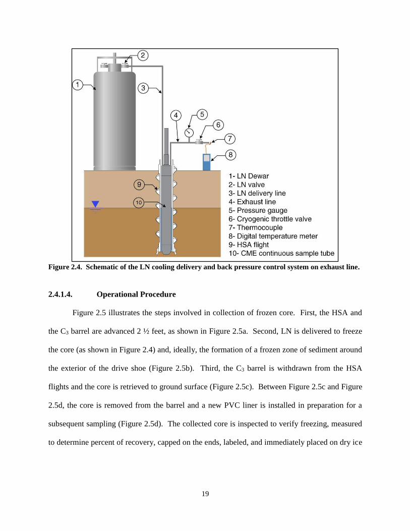
2.4.1.3. Coolant, Delivery, and Exhaust

Liquid nitrogen (LN), which provides temperatures as low as -196 ˚C at atmospheric

pressure, is used as a coolant. 160-liter LN Dewars with 230 psi internal pressure are employed.

A ¾-inch vacuum jacket tube connects the LN Dewar to the downhole delivery line. Delivery

and exhaust lines consist of 5-foot long, ¾-inch OD sections of stainless-steel tubes, insulated

with 1/4-inch closed-cell neoprene insulation and covered with heat-shrink PVC tubing. The 5-

foot sections are connected with stainless-steel SwagelokTM unions.

A cryogenic throttle valve and pressure gauge are placed on the exhaust line above

ground surface to control back pressure in the cooling systems (Figure 2.4 and Figure A-4).

Optimal cooling is achieved by 1) maintaining about 200 psi at the Dewar, 2) initially imposing

zero back pressure at the exhaust in order to maximize flow, and 3) after 0 °C is observed at the

exhaust, closing the throttle valve to achieve a back pressure of approximately 100 psi in the

exhaust line to maintain the nitrogen in a liquid state adjacent to the core.

19

Figure 2.4. Schematic of the LN cooling delivery and back pressure control system on exhaust line.

2.4.1.4. Operational Procedure

Figure 2.5 illustrates the steps involved in collection of frozen core. First, the HSA and

the C3 barrel are advanced 2 ½ feet, as shown in Figure 2.5a. Second, LN is delivered to freeze

the core (as shown in Figure 2.4) and, ideally, the formation of a frozen zone of sediment around

the exterior of the drive shoe (Figure 2.5b). Third, the C3 barrel is withdrawn from the HSA

flights and the core is retrieved to ground surface (Figure 2.5c). Between Figure 2.5c and Figure

2.5d, the core is removed from the barrel and a new PVC liner is installed in preparation for a

subsequent sampling (Figure 2.5d). The collected core is inspected to verify freezing, measured

to determine percent of recovery, capped on the ends, labeled, and immediately placed on dry ice

20

in a cooler. All frozen core was shipped to Colorado State University (CSU) and stored in a

walk-in -20 °C refrigeration room.

A notable complication was, for some cores, the core liners were frozen to the cooling

coil or dual-wall cooling cylinder. This challenge was resolved by running hot water from a

pressure washer for less than 20 seconds through the cooling systems to thaw the film of ice

holding the core in the system.

Figure 2.5. C3 operational procedure a) advancement of the HSA and the C3 barrel, b) injection of LN through the C3 system to freeze the core and the formation immediately below the drive shoe, c) withdrawal of the C3 barrel to the surface and recovery of core, and d) the HSAs and the C3 barrel are advanced for the next interval.

2.4.2. Controlled Experiments of Freezing Time

To evaluate the time required to freeze sediment core in situ, a series of controlled

experiments were conducted at the Drilling Engineers, Inc. facility in Fort Collins, CO. To

accomplish these experiments, PVC liner was packed with sand (sand, moderately sorted, silt to

21

fine sand) and saturated with tap water. The pre-packed core was equipped with Type K

thermocouples located at the top, middle, and bottom. The thermocouples were connected to a

4-channel temperature logger (Omega HH378 temperature meter). The pre-packed core was

placed inside the C3 barrel and lowered into 10 feet, as well as 20 feet, of 4 ¼-inch ID HSA

flight that had been drilled in the ground. Freezing of the pre-packed core was then carried out

as described previously (with 200 psi at the LN Dewar and, in this case, with no back pressure at

the exhaust), and the temperatures were recorded as a function of time.

2.4.3. Application of the C3 Method at Field Sites

Application of the C3 method at two contaminated field sites are discussed briefly here

and have been discussed in greater detail by Sale et al. (2015). Samples were first collected at

F.E. Warren (FEW) Air Force Base on September 22 and 23, 2014. FEW is an approximately

7000-acre facility, consisting of shallow of eolian and fluvial deposits. Eolian deposits include

local beds of caliche. Eolian and fluvial deposits are underlain by the Ogallala formation.

Locally, the Ogallala formation consists of interbedded gravel, sand, and silt beds with varying

clay content. Through historical maintenance and disposal activities, chlorinated solvents

(primarily TCE) were inadvertently released to the subsurface.

Two different field mobilizations were carried out at the former refinery site in the

western U.S. (September 30, 2014 and August 11 and 12, 2015). The former refinery covers

approximately 200 acres and is underlain by North Platte River alluvium. Sediments grade from

fine-grained over bank deposits (sand and silts) at ground surface into point bar sands and

channel gravels with depth. Beds of gravels and cobbles are also present within the over bank

and point bar deposits. The site is impacted by historical releases of petroleum associated with

petroleum refining operations between 1923 and 1982.

22

2.4.4. Core Analysis

A critical aspect of C3 is the analysis of the core. The process of sub-sampling,

preserving sub-samples, and sample analyses is referred to here as ″high-throughput analysis

(HTA)″. The methods of HTA have been documented by Sale et al. (2015) and will be briefly

discussed here. The combined processes of C3 and HTA allow all core processing to be

conducted in the laboratory, versus in the field, and on a timeframe that is flexible (i.e., because

the core is kept frozen). Other advantages of laboratory processing include 1) elimination of

weather-related sample biases, 2) access to better environmental and safety controls (e.g., hoods,

gloves, etc.), 3) improved accuracy of measurements (e.g., weights and volumes), and 4)

enhanced safety associated with not deploying staff to field sites.

As discussed above, frozen core can be used to examine a broad set of physical,

chemical, and biological characteristic of sediments. As an example of these results, distribution

of fluid saturation (i.e., water, non-aqueous liquid, and gas) of frozen core collected from the

former refinery is reported in the following Results section. However, other parameters for

which analysis can be improved by in situ freezing of sediment core, including volatile organic

compounds, redox-sensitive inorganic water-quality indicators (Fe2+, H2, H2S, O2) and minerals

(e.g., FeS), and microbial ecology, are reported in Sale et al. (2015).

Frozen core collected from four locations (E1D, B2D, B3D, and D4D) at the former

refinery (in August 2015) is cut into 1-inch (25.4-mm) sub-sections, referred to as ″hockey

pucks,″ at 4-inch intervals using a circular chop saw. Subsequently, hockey pucks were

quartered to sub-samples and preserved. Two of the sub-samples were used in the current HTA.

The 3-inch core section from between the hockey pucks was also stored in freezer for subsequent

analyses. Additional information regarding sub-sampling is presented in Sale et al. (2015).

23

Sediments were visually logged after HTA of sub-samples by a professional geologist

following the guidelines for hydrogeological logging of samples presented in Sterret 2007.

Recorded attributes include sediment type, sorting, grain-size distribution, color, and presence of

NAPL. Florescence induced by ultra-violet (UV) light was used to resolve the presence of

LNAPL (Cohen et al., 1992).

Concentrations of total petroleum hydrocarbons (CTPH) of sub-samples were determined

using solid-liquid extraction followed by gas chromatography (GC). Details of the method are

provided in APPENDIX A and are well described in Sale et al. (2015). Given concentration of

total petroleum hydrocarbons, Ccut-off is referred to as ″cut-off concentrations″ in which LNAPL

was observed in sub-samples under UV light above this concentration. Consequently,

concentration of LNAPL (CLNAPL) of sub-samples was determined by subtracting Ccut-off from

CTPH. Equations (2.1) through (2.6) present the determination of porosity, fluids saturation, and

fluids content of frozen core.

dtd VM 1 (2.1)

OffCutTPHLNAPL CCC (2.2)

ddtLNAPLdLNAPLLNAPL MVMCS (2.3)

ddtLNAPLdLNAPLlw MVMCVS (2.4)

wLNAPLg SSS 1 (2.5)

S (2.6)

where ϕ is porosity, M is mass (M), V is volume (L3), ρ is density (M/L3), C is concentration

(M/M dry sediment), S is saturation, and ω is fluid content. Subscripts d, l, w, g, and t refer to dry

sediment, liquids (i.e., water and LNAPL), water, gas, and total, respectively. Determination of

24

Md, Vt, and Vl is described in detail in Sale et al. (2015). In this study, the ρd and ρLNAPL were

assumed to be 2.65 and 0.8 g/cm3, respectively.

2.5. Results and Discussion

2.5.1. Rate of Cooling Experiments

Temperature and the rate of cooling versus time data, collected during the development

of the C3 method, is shown in Figure 2.6. In this case, approximately 6.5 minutes were required

to completely freeze a pre-packed core. The data were collected from a controlled experiment at

20 feet below the ground surface (water table at 10 feet). The experiment was performed using

the cooling coil system. In Figure 2.6, the cooling rate curve shows four steps through freezing

the pre-packed sediment core. First, the thermal diffusion front reaches the thermocouple at the

center of the core. Second, the cooling rate is controlled by the heat of fusion of water. Third,

the cooling rate slows slightly as the freezing front approaches the thermocouple. Last, the

cooling rate increases rapidly after the core is completely frozen.

Figure 2.6. Example data for the cooling experiment a) the thermal diffusion front reaches the thermocouple at the center of the core, b) the cooling rate is controlled by water's heat of fusion, c) the cooling rate slows slightly as the freezing front approaches the thermocouple, and d) the cooling rate increases rapidly after the core is completely frozen.

25

2.5.2. Core Production and Recovery

Table 2.1 summarizes frozen core production and recovery data at FEW and the former

refinery using the C3 method. Through three field efforts and five days of drilling, 146 feet of

frozen core were collected. The average cryogenic core production rate was about 30 foot/day.

Based on prior HSA coring at both sites, C3 requires approximately one and half as much time as

traditional HSA drilling. This observation needs to be balanced by the facts, described in the

following sections, that recovery from targeted intervals was improved using the C3 method and

key attributes, including fluid saturations, were preserved.

Table 2.1. Core production and production rate using C3 at FEW and the former refinery Site Dates Core Production

(foot) Core Production Rate

(foot/day) FEW September 22 & 23, 2014 50 25 Former refinery September 30, 2014 36 36 Former refinery August 11 & 12, 2015 60 30 Total 146 29

Core sample recoveries from field work at FEW and the former refinery sites are shown

in Figure 2.7. At FEW, except for intervals encountering caliche beds that required a center head

in lieu of the continuous sample tube system, recovery was close to 100%. At the former

refinery, recovery varied from 16% to 100% with a median of 80%. The primary factor limiting

recovery at the former refinery was cobbles that were larger than the 2 ½-inch ID drive shoe that

blocked sediment entry into the sample systems. As a basis of comparison, attempts to collect

sediment core at the former refinery site, using the 2 ½-inch ID CME continuous sample tube

system without the cryogenic cooling system consistently yielded extremely poor recovery (less

than 15%). Also, the time of injecting LN through the system to freeze the core is presented in

Figure 2.7. Using the C3 method, an average of five minutes of injecting LN was enough to

freeze a 2 ½-foot core above and below the water table.

26

Figure 2.7. Core recovery and time of LN injection through the C3 system at a) FEW (three locations: M173, M38, and M700) and b) the former refinery (four locations: E1D, B2D, B3D, and D4D).

On several of the core collection runs at the former refinery, control of flowing sand was

evaluated by measuring the solids level in the HSA after removal of the C3 barrel. This level

was compared to prior drilling at the same location when the C3 method was not used.

Preliminary results indicated that the dual-wall cooling system reduced the amount of sediment

entering the barrel between core collection runs. Future work will focus on more rigorous

evaluation of the potential to control flowing sand via freezing sediment below the drive shoe.

FEW-M173 FEW-M38 FEW-M700

Former Refinery-E1D Former Refinery-B2D Former Refinery-B3D Former Refinery-D4D

Recovery (%) Recovery (%) Recovery (%) Recovery (%)

Inte

rval D

epth

(ft)

Inte

rval D

epth

(ft)

Recovery (%) Recovery (%) Recovery (%)

Time of LN Injection (min) Time of LN Injection (min) Time of LN Injection (min)

Time of LN Injection (min) Time of LN Injection (min) Time of LN Injection (min) Time of LN Injection (min)

Recovery (%)

Time of LN Injection (min)

27

2.5.3. Core Analysis

2.5.3.1. Visual Logging of Sediments

Visual logs of the sediments collected from four locations (i.e., E1D, B2D, B3D, and

D4D) at the former refinery (in August 2015) are presented in Figure 2.8 and Figure 2.9. As is

typically seen in stream deposits, sediment generally grade from fine to coarse with depth.

Sediment colors graded from reds and browns above four feet to gray and black sediments below

four feet. Reds and browns are attributed to oxidized iron minerals. Grays and blacks are

attributed to reduced metal sulfides associated with anaerobic degradation of petroleum

hydrocarbons (Irianni Renno et al., 2015).

2.5.3.2. Fluid Saturation, Fluid Content, and Porosity

Figure 2.8 also shows fluid saturation, fluid content, and porosity of frozen core collected

from the former refinery (in August 2015). Critically, given in situ freezing, the results are not

biased by drainage of pore fluids from the core during sample collection. Median fluid content,

fluid saturation, and porosity values, above and below the water table, are summarized in Table

2.2. Lower porosity values reflect samples where large pieces of solid aggregate comprised a

large fraction of the sample. Large gas content/saturation below the water table is attributed to

gases being generated by anaerobic natural source zone depletion processes (Amos and Mayer

2006; Irianni Renno et al., 2015).

28

Figure 2.8. Results of fluid saturation, fluid content, and porosity determined after high-throughput analysis of frozen cores collected from E1D and B2D at the former refinery (August 2015).

Fo

rmer

Refi

nery

-B2D

Fo

rmer

Refi

nery

-E1D

Silt, moderately sorted,

silt to fine sand

Silt, well sorted, silt

Sand, well sorted,

fine sand

Sand, moderately sorted,

silt to fine sand


fine to medium sand


medium to coarse sand

Sand, poorly sorted,

silt to medium sand


silt to coarse sand


fine to coarse sand

LNAPL

Gas

Water

Porosity

Visible LNAPL

Water table

29

Figure 2.9. Results of fluid saturation, fluid content, and porosity determined after high-throughput analysis of frozen cores collected from B3D and D4D at the former refinery (August 2015).

Fo

rme

r R

efi

ne

ry-D

4D

Fo

rme

r R

efi

ne

ry-B

3D

Silt, moderately sorted,

silt to fine sand

Silt, well sorted, silt

Sand, well sorted,

fine sand


silt to fine sand


fine to medium sand


medium to coarse sand


silt to medium sand


silt to coarse sand


fine to coarse sand

LNAPL

Gas

Water

Porosity

Visible LNAPL

Water table

30

Table 2.2. Median porosity, fluid content, and fluid saturations of frozen core collected from the former refinery (August 2014)

Parameter

Median Results Volume / Volume Porous Media

Above the water table Below the water table Porosity 23.7 29.2 Water content/saturation 14.5/49.5 22.1/74.2 Gas content/saturation 10.8/50.5 5.8/22.9 LNAPL content/saturation 0.2/0.6 0.9/2.8

2.6. Summary and Conclusions

This chapter documents a practical approach for collecting in situ frozen core from

unconsolidated subsurface media. Key elements of the C3 method include downhole circulation

of LN via a cooling system, strategic use of insulation to focus cooling into the core, and use of

back pressure to optimize cooling. The rate of core collection using the C3 method was

approximately 30 foot/day. Application of the C3 method improves core recovery and limits

potential biases associated with flowing sand. Furthermore, the C3 method improves

preservation of key attributes of sediments. In this case, frozen core was used to examine fluid

saturation, fluid content, and porosity. Critically, these attributes were examined without

drainage of pore fluids. Other sediment attributes that can benefit significantly from using

frozen core include microbial ecology, redox conditions, sediment mineralogy, and dissolved

gases. The overarching vision for C3 is that the expanded knowledge that can be derived from

frozen core will facilitate better resolution of subsurface contaminants, leading to enhanced site

conceptual models and site remedies.

31

CHAPTER 3

CRYOGENIC CORE COLLECTION AND HIGH-THROUGHPUT ANALYSIS OF FROZEN

CORE

Co-authors: Mitch Olson, Richard Johnson, Maria Irianni Renno, Jens Blotevogel, Thomas Sale


Third-generation (3G) site characterization methods have been developed by advancing

practical approaches to 1) cryogenic core collection (C3) and 2) laboratory high-throughput

analysis (HTA) of frozen core. The C3 method was applied at F.E. Warren (FEW) Air Force

Base (near Cheyenne, WY). FEW is impacted by historical release of chlorinated solvents.

Frozen core was collected from three locations that had been characterized in 2010 using second-

generation (2G) site characterization methods (i.e., Membrane Interface Probe (MIP), Waterloo

ProfilerTM, laboratory analysis of sub-samples provided from continuous sediment cores, and

multilevel sampling system). The frozen core collected by the C3 method was processed and

analyzed in a laboratory to acquire high-resolution, depth-discrete data of physical, chemical,

and microbial properties from the subsurface. The results illustrated the advantages of C3

including accurate recovery of sediments from targeted intervals and preservation of pore fluid

(both in dissolved and gas phases), microbial ecology, and mineralogy. Overall, C3 from

unconsolidated geological subsurface and HTA of frozen core in laboratory facilitates better

resolution of the occurrence of subsurface contaminants and biogeochemical conditions.

Critically, rigorous resolution of subsurface conditions is central to advancing enhanced site

conceptual models and selecting appropriate remedies.

32

3.2. Introduction

Modern contaminant hydrology is embracing the concept that decisions regarding

management of subsurface contamination in unconsolidated subsurface media require a holistic

understanding of contaminant distribution in all phases (i.e., aqueous, non-aqueous liquid,

sorbed, and gas), in both transmissive and low permeability (low-k) zones. Given the distinction

of source zones and plumes (NRC 2005), contaminant concentrations need to be resolved in 14

compartments as illustrated in Figure 3.1 (Sale et al., 2011). Going a step further, resolution of

biogeochemical conditions in each of the 14 compartments, is critical. Biogeochemical

conditions associated with all compartments are central to understanding natural losses of

contaminants as well as the efficacy of active remedial measures.

Figure 3.1. 14 subsurface compartments of contaminants. Arrows show mass potential transfer links between compartments. Dashed arrows indicate irreversible fluxes (Sale et al., 2011).

Historically, the primary tools for characterizing subsurface releases have been

groundwater monitoring wells and grab sediment samples, referred to as ″first generation (1G)″

methods. 1G methods provide limited insight regarding conditions in most of the 14

compartments presented in Figure 3.1. As demonstrated by Guilbeault et al. (2005) and shown

in Figure 3.2, wells commonly collect water samples at a scale that is larger than the elemental

volume to which a single aqueous concentration can be attributed. Furthermore, due to the

33

preferential recovery of water from transmissive zones, wells provide little if any knowledge

regarding aqueous concentrations in low-k zones. Absent non-aqueous phase liquid (NAPL),

water samples from wells with long screens at best describe aqueous concentrations in

transmissive zones of source zones and plumes, only two of the 14 potentially relevant

compartments introduced in Figure 3.1. Common limitations of grab sediment samples center on

the loss of sediment during withdrawal, ineffective preservation of samples due to drainage and

redistribution of pore fluids, invasion of atmospheric gases during sample recovery, and losses of

volatile compounds (Sale et al., 2015; Kiaalhosseini et al. 2016).

Figure 3.2. A monitoring well screened above an aquitard in a heterogeneous alluvial deposit with aqueous contaminant concentrations (Guilbeault et al., 2005).

Limitations of 1G site characterization methods have led to the second generation of

high-resolution site characterization methods (2G methods). Following Sale et al. (2013),

common 2G methods include multilevel sampling system, Waterloo ProfilerTM, Membrane

Interface Probe (MIP), and high-resolution sub-sampling of sediment core. Given favorable

hydrogeological conditions, the 2G approach provides high-resolution discretization of aqueous

Aqueous Conc. (μg/L)

34

concentrations, overcoming the limitations of vertically-integrated water samples from

conventional monitoring wells. In addition, all of the methods except MIP provide correlated

data regarding the occurrence of transmissive and low-k zones. Of the four methods, only high-

resolution sub-sampling of core and analysis of the sub-samples has the potential to resolve

concentrations of gas, NAPL, and sorbed phases, microbial ecology, and mineralogy.

In this study, cryogenic core collection (C3) with laboratory-based high-throughput

analysis (HTA) of frozen core is advanced as third generation (3G) approaches to site

characterization. Following Kiaalhosseini et al. (2016), advantages of collecting frozen core

include improved core recovery, retention of pore fluids, and preservation of critical properties.

Historically, the collection of frozen core has seen wide attention (Yoshimi et al., 1984;

Durnford et al., 1991; Murphy and Herkelrath 1996; and Johnson et al., 2013). However, none

of the proposed methods for in situ freezing of core has been sufficiently practical to see

widespread use. Herein, novel methods for C3 are described. These methods involve circulation

of liquid nitrogen (LN) to a downhole core collection system within a hollow-stem auger system.

Furthermore, novel methods for laboratory analysis of frozen core are advanced to provide high-

resolution, depth–discrete data of subsurface conditions. Finally, a comparison between the

results of site characterization using 2G methods applied in 2010 and 3G methods applied in

2015 at F.E. Warren (FEW) Air Force Base (in Cheyenne, WY) is presented.


The overarching objective of this study is to 1) demonstrate novel methods for C3, 2)

document methods for HTA of frozen core, and 3) provide a comparison of results using 2G and

3G methods in chlorinated solvent plumes. The following hypothesis will be tested in this study:

35




3.4. Methods

This section describes 3G site characterization study conducted at F.E. Warren (FEW)

Air Force Base (in Cheyenne, WY) in September of 2014. 3G methods that were applied at

FEW include C3 and laboratory HTA of frozen core. In November 2010, 2G methods were

employed including the application of Membrane Interface Probe (MIP), Waterloo ProfilerTM,

laboratory analysis of sub-samples provided from continuous sediment core, and multilevel

sampling system that are described in Sale et al. (2013). FEW is an approximately 6,000-acre

facility underlain by shallow eolian and fluvial deposits with local beds of caliche. Eolian and

fluvial deposits are underlain by the Ogallala formation. Locally, the Ogallala formation consists

of interbedded gravel, sand, and silt beds with varying clay content. Through historical

maintenance and disposal activities, chlorinated solvents (primarily TCE) were inadvertently

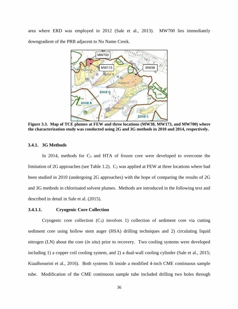
released to the subsurface (Sale et al., 2006). Figure 3.3 presents a map of TCE plumes and three

locations where the 2G and 3G methods were applied in 2010 and 2014, respectively.

Over the past 40 years, TCE concentrations at the site have been stable in the range of

high tens to low hundreds of micrograms per liter (µg/L). MW38 lies in a plume 1000s of feet

from the suspected source area. MW173 and MW700 are located in areas referred to as ″Spill

Site 7″. Following Sale et al. (2013), sequential applications of excavation, soil vapor extraction

(SVE), iron permeable reactive barrier (PRB), and enhanced reductive dechlorination (ERD) at

Spill Site 7 have failed to address TCE concentrations in excess of maximum contaminant levels

(MCLs) in a down-gradient creek (No Name Creek). MW173 lies up-gradient of the PRB in an

36

area where ERD was employed in 2012 (Sale et al., 2013). MW700 lies immediately

downgradient of the PRB adjacent to No Name Creek.

Figure 3.3. Map of TCE plumes at FEW and three locations (MW38, MW173, and MW700) where the characterization study was conducted using 2G and 3G methods in 2010 and 2014, respectively.

3.4.1. 3G Methods

In 2014, methods for C3 and HTA of frozen core were developed to overcome the

limitation of 2G approaches (see Table 1.2). C3 was applied at FEW at three locations where had

been studied in 2010 (undergoing 2G approaches) with the hope of comparing the results of 2G

and 3G methods in chlorinated solvent plumes. Methods are introduced in the following text and

described in detail in Sale et al. (2015).

3.4.1.1. Cryogenic Core Collection

Cryogenic core collection (C3) involves 1) collection of sediment core via cutting

sediment core using hollow stem auger (HSA) drilling techniques and 2) circulating liquid

nitrogen (LN) about the core (in situ) prior to recovery. Two cooling systems were developed

including 1) a copper coil cooling system, and 2) a dual-wall cooling cylinder (Sale et al., 2015;

Kiaalhosseini et al., 2016). Both systems fit inside a modified 4-inch CME continuous sample

tube. Modification of the CME continuous sample tube included drilling two holes through

37

driving head to pass the LN delivery and exhaust lines through the system and a custom-design

drive shoe to provide clearance for the cooling system placed in the drive shoe. Insulation was

placed around the cooling systems to focus cooling into the sediment core. To achieve optimal

cooling, a back-pressure control system was installed on the exhaust line at the surface.

In September of 2014, the C3 method was applied at three locations (MW38, MW173,

and MW700) at FEW over two consecutive days. Continuous frozen core was collected at a 5-

foot offset from the locations that were studied in 2010 using 2G methods. The C3 procedure is

illustrated in Figure 3.4. The HSA and the C3 barrel were advanced 2 ½ feet, as shown in Figure

3.4a. Following, LN is delivered to freeze the core and, ideally, creates a frozen zone under the

drive shoe (Figure 3.4b). Next, the C3 barrel is withdrawn from the HSA flights, and the core is

retrieved from the sample barrel (Figure 3.4c). The collected core is inspected to verify freezing

and to determine the percent of sediment recovery. The core is capped on the ends, labeled, and

immediately placed on dry ice in a large cooler to be shipped to the laboratory (Kiaalhosseini et

al., 2016). At the laboratory, all frozen core is placed in a freezer room at

-20 °C.

38

Figure 3.4. The C3 operational procedure: a) advancement of the HSA and the C3 barrel, b) injection of LN through the C3 system to freeze the core and the formation immediately below the drive shoe, c) withdrawal of the C3 barrel to the surface and recovery of core, and d) advancement of the HSAs and the C3 barrel for the next interval (Kiaalhosseini et al., 2016).

3.4.1.2. High-Throughput Analysis

As a complement to C3, high-throughput analysis of frozen core was developed to

process the frozen core rapidly. The HTA consisted of core processing to provide sub-samples,

preserving sub-samples, and analysis of sub-samples for parameters of concerns. Figure 3.5

illustrates the HTA of frozen core in the laboratory as a flow chart.

39

Figure 3.5. High-throughput analysis (HTA) of frozen core in the laboratory.

3.4.1.2.1. Core Processing

Cutting the frozen core was the first step of core processing (Figure 3.6). Each 2 ½-foot

frozen core was cut into 1-inch thick discs (referred to as ″hockey puck″) using a chop saw

(Hitachi, Diablo “Metal Cut-Off” blade, with 14-inch diameter and 1/8-inch thickness) in a fume

hood (Figure 3.6a). Hockey pucks were collected every four inches (Figure 3.6b). To gauge the

lengths of frozen core for each cut quickly, hand-held stop-blocks were used. Each hockey puck

was placed in the splitting device and quartered into four sub-samples using a hammer and chisel

40

according to the pattern shown in Figure 3.6c. One quarter was used for methanol extraction.

Another quarter was used for water extraction. The last two quarters were wrapped in aluminum

foil and stored in a freezer, one for microbial analysis and the other for an archive sample. The

core processing was critical to avoid thawing sub-samples before extraction. The remaining 3-

inch segments of frozen core in between hockey pucks were stored in a freezing for permeability

testing.

Figure 3.6. Core processing: a) cutting frozen core in a fume hood, b) 1-inch thick hockey pucks collected for every four inches of each core, c) splitting hockey pucks into four quarters for 1) methanol extraction, 2) water extraction, 3) microbial analysis, and 4) future analysis.

3.4.1.2.2. Preserving Sub-Samples

3.4.1.2.2.1. Methanol Extraction

A quarter of each hockey puck was extracted in methanol for volatile organic compounds

(VOCs) analysis, targeting perchloroethylene (PCE), trichloroethylene (TCE), dichloromethane

(DCE) isomers, and vinyl chloride (VC). These extractions were emplaced in 120-mL glass jars

with PTFE-lined caps filled with 80 mL of high-purity (99.9%) methanol (Burdick & Jackson).

Weights before and after adding the sub-samples into the jars were recorded. The sample jars

41

were placed on a vortex shaker for about 15 minutes to disperse sediments. The sample jars

were then stored in a refrigerator (about 4°C) for at least four days, providing time for slowly-

desorbing contaminants to partition into the methanol. Finally, an aliquot of the methanol

extracts was transferred into 2-mL GC vials for analysis.

3.4.1.2.2.2. Water Extraction

A quarter of each hockey puck was also extracted in water for VOCs analysis, targeting

the lower-molecular-weight products including methane, ethane, and ethene. 120-mL

borosilicate glass jars with PTFE-lined septa caps were filled with de-aired, de-ionized water

(provided by a Barnstead Thermolyne NanoPure®DiamondTM UV ultrapure water system) with

no head space under anaerobic condition in an anaerobic chamber. The sub-samples were placed

in the water extraction jars. Since the jars were completely filled with DI-water, the sub-samples

displaced water from the jars. The jar lids then were replaced, thus re-sealing the jars with no

headspace (with the exception of gas phases that may have been entrapped in the frozen sub-

sample). Weight of the extraction jars before sampling, the extraction jars with the sample and

displaced water, and the displaced water were recorded. The displaced water weight was used to

estimate sample density. The sample jars were placed on a vortex shaker for about 15 minutes to

disperse solid materials. The jars were then stored in a refrigerator (4°C) for an equilibration

time of at least four days. The water extract was transferred into 20-mL headspace vials

constructed of borosilicate glass. The vials then were sealed with crimp-style PTFE-lined septa

caps. A transfer method was developed that allowed for the transfer of water from water-extract

jars into the headspace vials with no atmospheric exposure. This method is described in

APPENDIX B. The remaining water in the extract vial was subsequently used for inorganic

analysis, pH, and ORP measurements. The water extract jars were returned to the refrigerator to

42

preserve conditions for these analyses. The headspace vials were analyzed within 24 hours of

transfer.

3.4.1.2.3. Geology Logging

Geologic logging was conducted based on visual observation of the sub-samples residing

in the methanol extract jars upon completion of all analysis. Sub-samples were visually logged

for properties including sediment type, sorting, grain size, color, and description. The geologic

logging was performed by a registered professional geologist.

3.4.1.2.4. Organic Compounds Analysis

The methanol extracts were analyzed using two methods. Method 1 was used to provide

low detection limits for the highly-chlorinated compounds (i.e., PCE and TCE) and method 2

was used to provide higher detection limits for the degradation products (i.e., DCE isomers and

VC). Method 1 employed an Agilent 6890 GC with an electron-capture detector (ECD). The

GC is equipped with a J&W Scientific DB-5 column (30 m length, 0.32 mm ID, and 0.25 μm

film thickness). Injection parameters consisted of a 5:1 split ratio and a column flow rate of 3.0

mL/min. The GC temperature was initially held for three minutes at 40 °C, ramped at 10 °C/min

to 50 °C, ramped at 40 °C/min to 120 °C, and held for 1 minute. Method 2 was conducted using

an Agilent 6890 GC with a mass spectrometric (MS) detector. The GC/MS is equipped with a

Restek RXi®-624Sil MS column (30 m length, 0.25 mm ID, and 1.4 μm film thickness).

Injection parameters consisted of a 4:1 split ratio and a column flow rate of 3.0 mL/min. The GC

temperature was initially held for two minutes at 40 °C, ramped at 8 °C/min to 100 °C, ramped at

40 °C/min to 160 °C, and held for 1 minute. The MS detector was operated in single-ion mode

(SIM) for this analysis. For both methods, calibration standards for TCE, PCE, cis-1,2-DCE,

43

trans-1,2-DCE, 1,1-DCE, and VC were prepared in high-purity methanol. Five-point calibration

curves were included with each analytical sequence.

3.4.1.2.5. Dissolved Gas and Water-Extractable Volatile Organic Compounds

Water extracts were analyzed to detect VOCs with lower-molecular weight, including

methane, ethane, and ethene. Analysis of dissolved organic gas and water-extractable VOCs was

conducted on an Agilent 6890 GC with flame ionization detector (FID) with a Tekmar 7000

headspace autosampler. The samples were equilibrated in the autosampler at 80 °C for 15

minutes. The GC/FID was equipped with a Restek RT®-Q-BOND column (30 m length, 0.32

mm ID, and 10 μm film thickness). Injection parameters consisted of a 20:1 split ratio. The

initial column flow rate was held at 1.0 ml/min for 5.5 min and then was ramped at 12 mL/min to

4.0 mL/min. The GC temperature was kept at 45 °C for 5 min and then ramped at 20°C/min to

250 °C.

3.4.1.2.6. Inorganic Analysis

The inorganic analysis included the estimate of major anions and dissolved ferrous iron

in water extracts. Methods of analysis are described in the following.

3.4.1.2.6.1. Anions

Analysis for anions was performed using water extracts. After 10 days, 10 mL of the

water extracts were removed from select sample jars and transferred to the instrument-specific

Ion Chromatography (IC) vials. Analysis for anions was conducted on a Metrohm 861

Advanced Compact IC, equipped with a Metrohm A Supp 5 – 250 column. Calibration

standards for chloride (Cl-), bromide (Br-), nitrate (NO3-), phosphate (PO43-), and sulfate (SO42-)

were included in the analysis.

44

3.4.1.2.6.2. Ferrous Iron

The water extract was also analyzed for dissolved ferrous iron (Fe2+) using colorimetric

methods. A modified version of the Hach Co. Ferrous iron method (1,10-phenanthroline

method) was used. The manufacturer's instructions state to dissolve the contents of one reagent

pillow (Hach part #103769) in 25 mL of aqueous sample (i.e., 0.04 pillows/mL). Due to the

smaller volume of water available, a concentrated reagent solution was prepared with one

reagent pillow per 2.5 mL of DI water (0.4 packets/mL). Next, in a clear-plastic cuvette, 200 μL

of the concentrated reagent solution was added to 1800 μL of aqueous sample. This combination

provided 2 mL of sample for analysis, at a reagent concentration of 0.04 packets/mL, which is

equivalent to the manufacturer's instructions. Cuvettes were placed in a Thermo Scientific

Genesys 10 UV Spectrophotometer for analysis. Calibration solutions were included in the

analysis.

3.4.1.2.7. pH and ORP

The remaining water extract, after completion of the previous analysis, was used for pH

and ORP analysis. Note that dilution of pore water, which occurs during the water-extraction

procedure, is likely to affect the measured pH and ORP values. The pH values represent a

concentration, [H+], which can be corrected to a pore-water value by a simple dilution

relationship as follows:

C1V1=C2V2 (3.1)

where C and V refer to concentration and volume, respectively. Subscripts 1 and 2 refer to the

stock and diluted solutions, respectively. However, ORP refers to a potential, not a

concentration, so a dilution-based correction is not applicable. Although the reported ORP

45

values may not directly indicate in situ conditions, the relative ORP values provide an indication

of regions in the subsurface where conditions are relatively oxidizing or reducing.

pH and ORP were measured in each of the water-extract jars shortly after samples were

collected for VOC analysis. Vial lids were opened in a fume hood, and were thus exposed to

oxygen, which could affect ORP. Measurements were taken quickly (i.e., within 5 minutes) after

opening the vial caps to minimize the impact of atmospheric oxygen. pH and ORP were

measured using combination electrodes (VWR 89231-604 and VWR 89231-640, respectively)

with Ag/AgCl as the internal reference. For both pH and ORP, the electrodes were connected to

Denver Instruments UP-25 meters.

3.4.1.2.8. Fraction of Organic Carbon, Aqueous, and Sorbed Phase

Sub-samples in water-extract jars were used to determine the fraction of organic carbon

(foc) of the frozen core. To obtain foc data, all samples were analyzed for total- and inorganic-

carbon fractions. Organic carbon was then calculated by difference. First, excess water was

decanted from the water-extract jars and sub-samples were oven-dried at 80 °C overnight. The

dry weight was measured to determine sub-sample water content. Next, all of the dried sub-

samples were ground to a fine powder using a ball mill. The powder was then removed for total

carbon and inorganic carbon analysis. Total carbon was measured at the EcoCore facility

(Colorado State University (CSU), Fort Collins, CO) using a LECO Tru-Spec CN analyzer (Leco

Corp., St. Joseph, MI). Inorganic carbon was measured using an acid-digestion method.

Given foc, aqueous phase concentrations (Caq) and sorbed phase concentrations (CSorbed)

can be determined based on the following equations:

ococb

w

taq

KfS

CC

(3.2)

46

aqococsorbed CKfC (3.3)

where Ct is the total contaminant concentrations, ϕ is porosity, Sw is water saturation, ρb is bulk

density, and Koc is the organic carbon-water partitioning coefficient. ρb and w were determined

for water-extract sub-samples after completion of all analyses. The total mass and volume of

sub-samples were measured at the time of preserving sub-samples. To calculate w, the mass of

dry sediment was obtained from oven-dried sub-samples at 80 °C overnight.

3.4.1.2.9. Permeability

A core-in-liner (CIL) method was developed to measure the permeability of frozen core

collected at FEW. The CIL method was designed to measure the permeability of core directly in

the PVC liner without the need to remove the core. This method allows for permeability

measurements under in situ conditions, preserving cryogenically-collected core. In the

permeability tests, 3-inch segments of frozen core stored after core processing were used. The

CIL method and apparatus are described in APPENDIX B. Constant-flow and/or falling head

methods were used to measure the permeability of the core. Frozen core segments were initially

tested using the falling head, and high-permeable core (K>10-5 cm/sec) was analyzed using a

constant-flow test. For all permeability testing, tap water (City of Fort Collins) was used as a

permeating fluid.

3.4.1.2.10. Microbial Analysis

A quarter of each hockey puck wrapped in aluminum foil was used for DNA extraction.

Following Irianni Renno et al. (2015), DNA microbial analysis was performed in triplicate on the

sub-samples. To remove potential contaminants (e.g., humic substances), which can negatively

affect nucleic acid extraction yields as well as inhibit polymerase chain reaction (PCR) and

pyrosequencing reactions, core samples were pretreated as described in Whitby and Lund

47

Skovhus (2009) with a few modifications. 120 ng of skimmed milk was added per gram of

pretreated core sample instead of 80 ng. Polydeoxinocinic deoxicytidilic was added as an

aqueous solution, and the core sample combined with the polydeoxinocinic-deoxicytidilic

solution. The skimmed milk and 1 mL of distilled water were vortexed for one minute and

centrifuged prior to proceeding with the wash steps as indicated by the published protocol.

3.4.1.2.10.1. DNA

DNA was extracted from the pretreated sub-samples using the PowerlyzerTM Powersoil

DNA isolation kit (Mobio, Carlsbad, CA) per the manufacturer's specifications with the

following modifications: DNA yield was maximized by using 0.5 g of core instead of 0.25 g, and

duplicate extractions for each core sub-sample were pooled and processed with a single

PowersoilTM spin filter. Additionally, the volume of elution buffer was limited to 50 µl instead

of the recommended volume of 100 µl to increase DNA concentrations in the recovered volume.

DNA was quantified via optical density at 260 nm with a NanodropTM 2000 reader

(Thermoscientific, Wilmington, DE). DNA was extracted in triplicate from each core sub-

sample and stored at -20 °C prior to qPCR and pyrosequencing analysis.

3.4.1.2.10.2. qPCR Assays

SYBR greenTM (Life Technologies, Grand Island, NY) qPCR assays were used to

quantify the bacterial and archaeal 16S rRNA genes. Genomic DNA was extracted from

Desulfivibrio desulfuricans (ATCC #: 277740-5) and Methanosarcina acetivorans (ATCC #:

3595) was used to generate calibration curves for the bacterial and archaeal assays, respectively.

The primer sets 27F/388r and 931AF/1100Ar were used for amplification of bacterial and

archaeal 16S rRNA genes, respectively. All assays were performed using an ABI 7300 real-time

PCR system (Applied Biosystems, Foster City, CA). Each 25-μl SYBR greenTM qPCR reaction

48

contained: 1X Power SYBR greenTM 567 (Life Technologies, Grand Island, NY), forward and

reverse primers (2.5 μM), magnesium acetate (10 μM), PCR-grade water and 1 ng of DNA

template. Thermocycling conditions were as follows: 95˚C for 10 min, followed by 40 cycles of

95˚C for 45 s, 56˚C for 30 s, and 60˚C for 30 s. Dissociation curve analysis was conducted to

confirm amplicon specificity.

3.4.1.2.10.3. Pyrosequencing Analysis

Pyrosequencing analysis was performed by Research and Testing Laboratory, LLC

(Lubbock, TX), using an Illumina MiSeq/HiSeq Sequencer (Illumina, San Diego, CA). 16S

community profiling was performed targeting bacterial 16S rRNA genes with primers 28F and

519r and archaeal 16S rRNA genes with primers 519wf and 519r.


This section documents the results of C3 and laboratory high-throughput analyses at

FEW. Also, a comparison between the results of 2G and 3G methods performed at FEW is

shown and discussed in this section. More detail on the 2G results can be found in Sale et al.

(2013).

3.5.1. 3G Results

3.5.1.1. Cryogenic Core Collection

Fifty feet of frozen core was collected from FEW on September 22 and 23, 2014. The

average frozen core production rate was about 25 foot/day. Sample recovery was nearly 100%

for all of the drilling with the exception of caliche layers that required a center drill plug in lieu

of the continuous sample tube system. Time to freeze a 2 ½-foot core averaged five minutes,

above and below the water table (Kiaalhosseini et al., 2016). The water table was 14.5, 25, and

11.5 feet below ground surface (bgs) at MW38, MW173, and MW700, respectively. Sampled

49

intervals at MW38, MW173, and MW700 were at depths between 9 and 22.7, 14 and 38.2, and 9

and 17.5 feet bgs, respectively.

3.5.1.2. High-Throughput Analysis

3.5.1.2.1. Core Processing

We made every effort to minimize thawing of the frozen core. The typical time required

to process a 2 ½-foot frozen core was about 30 minutes, including cutting the hockey pucks and

splitting into the sub-samples.

3.5.1.2.2. Geology Logging

Geology logs of the core are shown in Figure 3.7a, Figure 3.8a, and Figure 3.9a.

Generally, site geologic media was comprised of fine-grained sediments, with particle sizes

primarily ranging from fine sand to silt. One of the key features of the site geology is the degree

of heterogeneity. Most of the geologic layers consisted primarily of fine sand with varying

degrees of sorting (well- to poorly-sorted). Layers of well-sorted to poorly-sorted silt were

identified, interbedded within the fine sand. Critically, subsequent analyses show that the

distribution of transmissive and low-k zones can be correlated with spatial variations in

contaminants, redox conditions, and foc in ways that hold promise for novel insight into

governing processes.

3.5.1.2.3. Organic Compounds Analysis

Methanol extracts were analyzed for PCE, TCE, DCE isomers, and VC concentrations.

The primary VOC detected was TCE, which was present in all sub-samples collected from the

three locations. PCE, trans-1,2-DCE, cis-1,2-DCE, 1,1-DCE, and VC were not detected in any

of the sub-samples. TCE concentrations versus depth for the three locations are shown in Figure

3.7b, Figure 3.8b, and Figure 3.9b. Given the low concentrations and large distances from

50

release areas, we assumed that no NAPL was present in any of the collected samples. For

MW38C, TCE concentrations ranged from non-detectable value (<5 μg/kg) to 41 μg/kg, with an

average value of 21 μg/kg. For MW173, TCE concentrations ranged from non-detectable value

(<5 μg/kg) to 108 μg/kg. The average of detected values was 38 μg/kg. TCE concentrations

greater than 50 μg/kg were observed at depths of 14.4, 19.2-20.1, 27.2, 30.8-33.6, and 37.2-39.0

feet bgs. TCE concentrations are generally lower in transmissive versus low-k zones, perhaps

reflecting preferential delivery of lactate (injected near MW173 in the late 2000s) to the

transmissive zone. The highest TCE concentrations were present in the sub-samples collected

from MW700. In this location, TCE concentrations ranged from 6 to 400 μg/kg and averaged

110 μg/kg. Elevated TCE concentrations were observed between 13.9 and 17.0 feet bgs. In

general, the results indicate fairly smooth trends with variable TCE concentrations versus depth.

These results are expected considering typical heterogeneous subsurface environments. The

earliest documentation of TCE at FEW (the U.S. Geological Survey (USGS), May and June

1987) indicates that TCE has persisted at FEW at detectable levels for more than 28 years.

Samples were also analyzed for PCE concentrations. PCE was detected above reporting

limits (about 7 μg/kg) in only one sub-sample collected from MW173, at a depth of 14.8 feet

(14.5 μg/kg). PCE was present below reporting limits in several sub-samples. Figure 3.7b,

Figure 3.8b, and Figure 3.9b shows the estimated quantities of PCE versus depth at three

locations.

3.5.1.2.4. Dissolved Gas and Water-Extractable Volatile Organic Compounds

Water-extracts were analyzed for methane, ethane, ethene concentrations. Only methane

was regularly detected in sub-samples as shown in Figure 3.7b, Figure 3.8b, and Figure 3.9b. In

MW38, methane concentrations were low (less than 1900 μg/kg) through depth. In MW173,

51

methane concentrations ranged from non-detectable value (about 900 μg/kg) to 17,000 μg/kg. In

this location, methane was observed in transmissive zones, potentially associated with lactate

injection near the monitoring well in the late 2000s. Higher concentrations of methane were

generally detected at greater depth (i.e., greater than 27 feet bgs). The highest detected methane

concentrations were at MW700 in a low-k zone. In MW700, methane concentrations ranged

from 4900 to 21,000 μg/kg. Figures 3.7b, 3.8b, and 3.9b indicate an inverse correlation between

methane and TCE at a depth below the water table. The source of methane could be degradation

of naturally occurring organic matters. Low concentrations of TCE through depth could be

dressed by the heterogeneity of the formation. However, there is no evidence to prove a

relationship between the inverse trend of methane, TCE, and geology.

52

Figure 3.7. The results of HTA of frozen core collected from MW38 at FEW.

53


54


55

3.5.1.2.5. Inorganic Analysis

3.5.1.2.5.1. Anions

Inorganic parameters including chloride (Cl-), nitrate (NO3-), and sulfate (SO42-) are

presented in Figure 3.7c, Figure 3.8c, and Figure 3.9c. In MW38C, chloride concentrations

ranged from 13 to 390 mg/L with an average value of 100 mg/L. Nitrate concentrations ranged

from non-detectable value (<2.0 mg/L) to 26 mg/L and averaged 15 mg/L. Sulfate

concentrations ranged from 14 to 150 mg/L with an average value of 51 mg/L. Bromide and

phosphate were not detected in any sub-samples. In MW173, chloride concentrations ranged

from 10 to 490 mg/L and averaged 130 mg/L. Nitrate concentrations ranged from non-

detectable value (< 2 mg/L) to 11 mg/L with an average value of 5.4 mg/L. Sulfate

concentrations ranged from 7.7 to 890 mg/L and averaged 137 mg/L. In MW700, chloride

concentrations ranged from 8.4 to 120 mg/L and averaged 37 mg/L. Nitrate concentrations

ranged from non-detectable value (<2.0 mg/L) to 5.0 mg/L with an average value of 3.3 mg/L.

Sulfate concentrations ranged from 3.3 to 48 mg/L and averaged 17 mg/L. Bromide and

phosphate were not detected in any sub-samples.

Elevated chloride levels may reflect historical reductive dechlorination of chlorinated

solvents in select intervals. The presence of nitrate suggests a plume that is not strongly reduced

from a redox perspective. High levels of sulfate may indicate intervals where reductive

dechlorination is inhibited by the preferential reduction of sulfate.

3.5.1.2.5.2. Ferrous Iron

Ferrous iron (Fe2+) data are shown in Figure 3.7c, Figure 3.8c, and Figure 3.9c. In

MW38, ferrous iron concentrations ranged from non-detectable value (< about 0.04 mg/L) to 10

mg/L. In MW173, ferrous iron concentrations ranged from non-detectable value (< about 0.04

56

mg/L) to 7.2 mg/L. In MW700, ferrous iron concentrations ranged from 1.1 to 110 mg/L. In

general, ferrous iron concentrations were higher at a shallower depth (i.e., < 14.5 feet bgs).

3.5.1.2.6. pH and ORP

The results of pH and ORP measurements in sub-samples that had been diluted in water

are shown in Figure 3.7e, Figure 3.8e, and Figure 3.9e. As stated in the methods section, dilution

of pore water, which occurs during the water-extraction, is likely to affect measured pH and ORP

values. In MW38, pH ranged from 8.2 to 8.8, and ORP ranged from 140 to 400 mV. In

MW173, pH ranged from 8.2 to 8.7, and ORP ranged from -80 to 150 mV. In MW700, pH

ranged from 7.8 to 9.0, and ORP ranged from -230 to 120 mV. Overall, pH values are constant

near 8.0 in all cases. ORP values suggest an absence of reducing conditions at MW38, more

reduced conditions at NW173, and a strong reducing conditions in shallow depth at MW700.

3.5.1.2.7. Fraction of Organic Carbon, Aqueous, and Sorbed Phase

The fraction of organic carbon (foc) is presented in Table B-1 of APPENDIX B. Reported

values range from 0 (below detection limits) to 4.0%, with an average value of 0.11%. By

location, average foc values were 0.14%, 0.057%, and 0.18% for MW38, MW173, and MW700,

respectively.

Aqueous phase concentrations (Caq) and sorbed phase concentrations (Csorbed) were

determined using Equation 3.2 and 3.3 by assuming that there is no NAPL in the formation,

water saturation Sw is equal to one, and the organic carbon-water partitioning coefficient (Koc) is

equal to 126 mL/g (Pankow and Cherry 1996). Bulk density and porosity values were calculated

for each sample based on measured sample volume and water content. The aqueous and sorbed

phase concentrations are also shown in Figure 3.7d, Figure 3.8d, and Figure 3.9d. The results

suggested that the vast majority of the contaminant mass is in aqueous phase with concentrations

57

ranging from 250 to 500 µg/L. MW38 and MW173 had the highest concentrations in the

transmissive zones since MW700 had the highest concentrations in the low-k zones.

3.5.1.2.8. Permeability

The results of permeability tests are shown in Table 3.1. The data indicate nearly a three-

order of magnitude variation in permeability values for the studied materials. Generally, the

materials with higher values of permeability are sand versus silt and well-sorted versus

moderately- or poorly-sorted.

Table 3.1. Permeability of select core segments collected from frozen core of FEW Core location Depth

(feet) Description K, CF1 (cm/s) K, FH 2 (cm/s)

MW 38 19.08 Sand, moderately sorted 7.8×10-3 - MW700 9.80 Sand, well-sorted 2.3×10-3 - MW700 10.53 Sand, poorly-sorted 1.6×10-3 - MW700 10.90 Sand, moderately-sorted 7.3×10-4 - MW 38 15.34 Silt, well-sorted - 5.2x10-5 MW38 21.94 Silt, moderately-sorted - 2.2×10-5 MW38 20.53 Silt, moderately-sorted - 3.5×10-6

1 Constant flow testing methods (K > 10-4 cm/s) 2 Falling head testing methods (K < 10-4 cm/s)

3.5.1.2.9. Microbial Analysis

Figure 3.10 presents the geology log, methane and TCE concentrations, number of 16s

rRNA genes per gram of solids for archaea and bacteria, and overall community composition of

microbial ecology at MW700. Two distinct intervals are identified: I) a moderately sorted silt

(low-k zone) with low TCE, high methane, and higher levels of 16s rRNA genes and II ) a fine-

grain, well-sorted sand (transmissive zone) with high TCE and low methane concentrations and

lower level of numbers of 16s rRNA genes. Figure 3.10d describes the overall microbial

community at MW700 based on five samples. The data suggest distinct microbial communities

I) in the low-k zone and II ) in the transmissive zone.

58

Figure 3.10. Microbial analysis of frozen core collected from MW700 (FEW in 2014) 1) geology log, 2) methane and TCE concentrations 3) 16s rRNA genes per gram of core for archaea and bacteria as a function of methane and TCE, 4) overall microbial community composition.

3.5.2. Comparison of 2G and 3G Methods at FEW

In 2010, 2G site characterization tools, including Membrane Interface Probes (MIPs),

Waterloo ProfilerTM, high-resolution sub-sampling from continuous sediment core, and

multilevel sampling system were employed at FEW adjacent to monitoring wells MW38,

MW173, and MW700. In 2014, cryogenic core was collected using the C3 method at 5-foot

offsets from the locations that were characterized using 2G methods in 2010. The purpose of

returning to the same locations in 2014 was a desire to compare the performance of 2G and 3G

site characterization methods.

Of the four methods employed in 2010, only field sub-sampling of sediment core

provided meaningful insight. The shortcomings of the other methods at FEW are described in

Sale et al. (2013). Figure 3.11 shows the total TCE concentrations versus depth at MW38,

MW173, and MW700, using data acquired from analysis of field sub-samples (2G, in 2010) and

59

HTA of frozen core collected by the C3 method (3G, in 2014). Given the fact that spatial

heterogeneity of the subsurface prevents a direct comparison of 2G and 3G, the results indicate

consistently higher TCE concentrations at all three locations using the 3G approach. Many

factors contribute to higher contaminant concentrations using cryogenic core collection

techniques. The most significant factor is the preservation of the sediment attributes, in

particular, pore fluids and VOCs in comparison to the unfrozen conventional sediment core

collected in 2010.

Figure 3.11. TCE data acquired from MW38, MW173, and MW700 at FEW using 2G (in 2010) and 3G (in 2014) methods.


The C3 method was applied at FEW in Cheyenne, WY in 2014. Subsequently, frozen

core was analyzed using laboratory high-throughput core analysis techniques. This site is

60

contaminated with chlorinated solvents (primarily TCE) that were inadvertently released to the

subsurface through historical maintenance and disposal activities. Three locations that were

characterized by 2G methods (in 2010) were studied using 3G methods in 2014.

2G methods used at FEW included Membrane Interface Probe (MIP), Waterloo

ProfilerTM, continuous sediment core collection and high-resolution sub-sampling from the core,

and installation of multilevel sampling system for monitoring the plume. 3G methods included

C3 and HTA of collected frozen core. The C3 method involved circulation of liquid nitrogen

(LN) about downhole hollow stem auger sampling systems to freeze the core in situ. HTA of

frozen core was developed to rapidly process a large amount of sub-samples taken from the

frozen core.

Following Sale et al. (2013), application of 2G methods indicated that only analysis of

preserved sample provided from high-resolution sub-sampling of collected core yields

consequential results. However, the limitation of conventional coring to preserve sediment

attributes remains, in particular, in transmissive zones. Also, flowing sand into the drilled space

can compromise the recovery of the targeted interval.

Through the application of C3 at FEW, 50 feet of frozen core were collected in two days

with the rate of 25 foot/day. An average of five minutes of injecting LN was employed to freeze

a 2 ½-foot core above and below the water table. Except for intervals encountering caliche

layers, recovery of the core was close to 100%. The recovered core was stored in large coolers

on dry ice and shipped to CSU overnight.

As the first step of HTA of frozen core in the laboratory, core processing including

cutting the frozen core into 1-inch thick hockey pucks at four-inches intervals was performed.

The hockey pucks were subsequently split into four quarters (sub-samples) and preserved in

61

methanol and water for organic compound analysis as well as inorganic analysis and parameters

of interests. The typical time required to process a 2 ½-foot frozen core was about 30 minutes.

Analysis of methanol and water extracts was performed to estimate concentration of

TCE, PCE, DCE isomers, VC, methane, ethane, and ethane using GC/ECD, GC/MS, GC/FID.

At MW38, TCE was detected with the concentrations less than 50 μg/kg. Methane

concentrations were low at MW38, and ORP values were higher than MW700 and MW173. At

MW173, TCE was detected at concentrations as high as 100 μg/kg. Methane was observed in

transmissive zones, potentially associated with lactate injection near the well in the late 2000s.

TCE concentrations were generally lower in transmissive versus low-k zone, perhaps reflecting

preferential delivery of lactate to the transmissive zone. ORP values were lower at MW173 than

MW38. At MW700, TCE concentrations were highest (~400 μg/kg) in the transmissive zone.

The highest detected methane concentrations were also at this location (~21,000 mg/kg) in the

low-k zone. Below the water table, an inverse correlation between methane and TCE suggests

active treatment in low-k zone.

Analysis of the core collected from the three locations at FEW in 2010 (following 2G

approaches) and in 2014 (following 3G approaches) indicated consistently higher TCE

concentrations at all three locations using the 3G methods. One significant factor contributing to

this observation is that cryogenic core collection from unconsolidated subsurface media

preserves pore fluids within the core. Overall, 3G approaches that employ a combination of C3

with HTA of the frozen core in laboratory leads to high-resolution, depth-discrete data

addressing contaminant concentrations, geochemical conditions, and microbial ecology. This

approach provides a basis to enhance site conceptual models and, consequently, to optimize the

remedial strategies.

62

CHAPTER 4

SPATIAL DISTRIBUTION ANALYSIS OF NON-AQUEOUS PHASE LIQUIDS IN POROUS

MEDIA USING NUCLEAR MAGNETIC RESONANCE: LABORATORY AND FIELD

STUDIES

Co-authors: Benjamin Kohn, Ted Watson, Thomas Sale, Jens Blotevogel


At contaminated field sites, an essential step toward optimizing remedial design is the

delineation of contaminant distribution in geological media. Conventional analysis of grab

sediment samples in the laboratory is a common method that leads to average estimates of

contaminant concentration in the select intervals. However, acquiring spatial contaminant

distribution and concentration within the sediment samples remains a key challenge. Therefore,

the objective of this chapter is to develop a practical approach that can qualitatively and

quantitatively resolve non-aqueous phase liquid (NAPL) distribution within saturated porous

media using a (liquid state) 1H-NMR method. In a laboratory-scale experiment, analysis of

NAPL distribution within a fabricated sediment core (Colorado silica sand) saturated with DI

water and trichloroethylene (TCE) as the model contaminant was conducted. Magnetic resonance

images of the core at -25 °C indicated that the NMR signals of water-bound hydrogen atoms

were selectively suppressed while the water was in solid state and the TCE was still liquid.

Quantification of NAPL distribution within the porous media was performed using a one-

dimensional NMR scanning method. However, accuracy in recovery of TCE mass existing

within the fabricated core was poor and suggested dependence on grain-size distribution. In a

field study at an LNAPL-contaminated site, downhole NMR logging tools (Javelin, Vista Clara,

63

Inc.) were used to discriminate NAPL and water, qualitatively, using short- and long-echo times.

However, this study was sensitive to the noise stemming from the active facilities in the vicinity

of the study area or from the power lines passing over the region. Despite the need for further

investigation to resolve quantification of NAPL distribution within the porous media, the novel

approach of suppressing NMR signals of water-bound hydrogen by freezing the core is a

promising alternative to conventional laboratory analysis, simplifying the sample processing of

frozen core collected by the cryogenic core collection (C3) method, and enabling a detailed

visualization of spatial NAPL distribution. Collectively, this approach offers substantial

improvement of site conceptual models, and consequently, remedial strategies.

4.2. Introduction

Characterization of contaminant distribution within porous media is an important step

toward improvement of site conceptual models and design of remedial measures. To date,

conventional analytical methods (e.g., solid-liquid extraction, followed by gas chromatography)

applied to homogenized grab sediment samples are the common means to resolve contaminant

distribution within porous media. However, these methods do not resolve the contaminant

concentration spatially and provide only an average of concentration within the homogenized sample

interval. NMR, as an emerging non-destructive scanning method, has potential to address pore

geometry of saturated porous media as well as three-dimensional spatial distribution of pore

fluids within the porous media (Watson and Mudra 1994; Coates et al., 1999; Ellis and Singer

2007). This chapter explores the capability of NMR to resolve the spatial distribution of non-

aqueous phase liquid (NAPL) within saturated porous media. In the following sections,

fundamental information on the theory of NMR is introduced, and literature pertaining to NMR

study of pore fluids (i.e., water, NAPL) within the porous media is reviewed. Also, research

objectives and tested hypotheses are described.

64

4.2.1. Theory of Nuclear Magnetic Resonance

The theory of nuclear magnetic resonance is introduced in this section. The following

sections discuss the basic principles of NMR, polarization, relaxation, spin echo, the pulsed field

gradient, and the relaxation mechanism of pore fluids within porous media.

4.2.1.1. Basic Principles of NMR

NMR functions by detecting the response of atomic nuclei to induced magnetic fields.

Detection of atomic nuclei by magnetic resonance can be made under two conditions: 1) the

nuclei must have an odd number of protons, or the sum of protons and neutrons should be an odd

number (e.g., 1H, hydrogen has one proton), and 2) the element is naturally abundant on Earth

(Table 4.1. ). Since most of the NAPL (e.g., TCE, gasoline, diesel, etc.) have hydrogen atoms,

1H-NMR is employed in this study. In contrast to solid NMR, which studies the nuclei

associated with molecules in solid phase, 1H-NMR studies the protons in liquid phase.

Table 4.1. Magnetic properties of 1H and 13C-the most frequent nuclei detectable via NMR (James 1998; Levitt 2008)

The 1H isotope is a small, positively charged nucleus (i.e., proton) with an associated

spin. Spin, which is an intrinsic property of protons, is a source of angular momentum called

″spin angular momentum″ (Levitt 2008). The spinning proton represents a current-carrying loop

that produces a magnetic moment (Coates et al., 1999; Ellis and Singer 2007). The spin angular

momentum and magnetic moment of the proton are in the same direction. The constant of

proportionality between spin angular momentum and magnetic moment is known as

″gyromagnetic ratio″ (Callaghan 2011), as follows:

Isotope Natural abundance of

isotope (%) Gyromagnetic ratio (γ, 106 rad s−1 T−1)

Frequency at 2.35T (ω/2π, MHz)

1H 99.98 267.522 100 13C 1.11 67.283 25

65

J (4.1)

where J is the spin angular momentum, µ is the magnetic moment, and is the gyromagnetic

ratio. The spin angular momentum is a vector. In the absence of a strong magnetic field, the

direction of angular momentum may point in any possible direction in space (Levitt 2008).

Figure 4.1 shows the axis of spin angular momentum of 1H, which is randomly oriented.

Figure 4.1. Randomly-oriented spin angular momentum of 1H protons in the absence of an external magnetic field.

If protons with magnetic moment are placed in an external magnetic field, a torque will

be exerted on the magnetic moment, causing the nuclear magnetic moment to precess about the

direction of the external magnetic field with a frequency given by the Larmor equation, as

follows (Figure 4.2, Farrar and Becker 1971):

0B (4.2)

2

f (4.3)

66

where f is Larmor frequency [Hz], ω is angular frequency [rad·sec-1], is gyromagnetic ratio

[rad·sec-1∙Tesla-1], and B0 is external magnetic field [Tesla]. Based on Equation (4.3), for a given

external magnetic field (B0), different nuclear species have different Larmor frequencies, as

shown in Table 4.1, for B0 = 2.35 Tesla.

Figure 4.2. Precession of a magnetic moment about an external magnetic field (B0) at Larmor frequency.

4.2.1.2. Polarization

Generally, an ensemble containing a large number of identical nuclei is studied in NMR.

Based on quantum mechanics, if protons (with spin number I=1/2) are subjected to an external

magnetic field (B0), they are forced into two energy states: a low-energy state and a high-energy

state (Zeeman Effect, Figure 4.3, Levitt 2008; Callaghan 2011).

Figure 4.3. Zeeman Effect.

67

Protons with a low-energy state spin up, and protons with a high-energy state spin down,

both are aligned with the external magnetic field (B0). The number of protons in two energy

states always differs by the Boltzmann distribution (Callaghan 2011). This difference in number

of protons in low- versus high-energy state forms a net macroscopic magnetization (M0, Figure

4.4, Farrar and Becker 1971).

Figure 4.4. Illustration of forming net magnetization (M0) in the presence of an external magnetic field (B0).

The macroscopic magnetization M0 is defined as the net magnetic moment per unit

volume. For the case of N number of protons per unit volume, the net magnetization is given by

Curie's Law, as follows (Coates et al., 1999):

02

22

0 )4(3)1(

BkT

IhNM (4.4)

where k is the Boltzmann constant, T is the absolute temperature (Kelvin), h is Planck's constant,

and I is the spin number of the nucleus in which 1H is equal to ½.

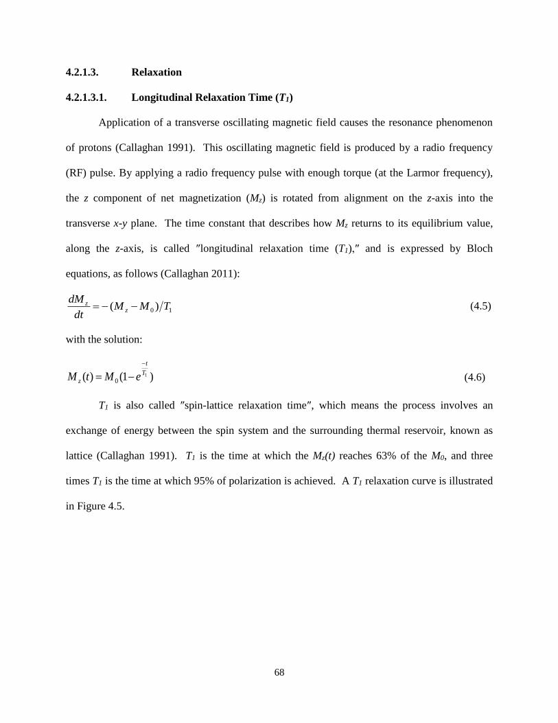
68

4.2.1.3. Relaxation

4.2.1.3.1. Longitudinal Relaxation Time (T1)

Application of a transverse oscillating magnetic field causes the resonance phenomenon

of protons (Callaghan 1991). This oscillating magnetic field is produced by a radio frequency

(RF) pulse. By applying a radio frequency pulse with enough torque (at the Larmor frequency),

the z component of net magnetization (Mz) is rotated from alignment on the z-axis into the

transverse x-y plane. The time constant that describes how Mz returns to its equilibrium value,

along the z-axis, is called ″longitudinal relaxation time (T1),″ and is expressed by Bloch

equations, as follows (Callaghan 2011):

10)( TMMdt

dMz

z (4.5)

with the solution:

)1()( 10

Tt

z eMtM (4.6)

T1 is also called ″spin-lattice relaxation time″, which means the process involves an

exchange of energy between the spin system and the surrounding thermal reservoir, known as

lattice (Callaghan 1991). T1 is the time at which the Mz(t) reaches 63% of the M0, and three

times T1 is the time at which 95% of polarization is achieved. A T1 relaxation curve is illustrated

in Figure 4.5.

69

Figure 4.5. T1 relaxation of protons: a) the external magnetic field is turned on at the time, ton, b) the T1 relaxation curve is being generated by polarization of protons after the time, ton.

4.2.1.3.2. Transverse Relaxation Time (T2)

The next step in the NMR cycle is to measure the decay of the net magnetization in the

transverse plane (x-y plane). After applying a 90° RF pulse to the proton population that is

already polarized (in the B0), the protons precess in phase in the transverse plane (x-y plane).

When the RF pulse is turned off, the proton population begins to come to thermal equilibrium

among itself, called ″transverse relaxation″ or ″spin-spin relaxation time (T2)″. The transverse

relaxation, known as ″free induction decay (FID)″, is shown in Figure 4.6 and is described as

follows (Callaghan 1991):

2T

M

dt

dM xyxy (4.7)

with the solution:

20)( T

t

xyxy eMtM (4.8)

where M0xy is the magnitude of the transverse magnetization at t = 0. However, during returning

to the thermal equilibrium, protons begins to de-phase or lose phase coherency. This

phenomenon decreases detection of NMR signals.

70

Figure 4.6. T2 relaxation of protons a) the RF pulse is turned off at the time, toff, b) T2 relaxation curve is being generated as the FID after the time, toff.

4.2.1.4. Spin Echo

As discussed above, by applying a 90° RF pulse, the proton population is forced to

precess in phase in the transverse plane. The coherent precession of protons creates a signal that

is detectable. However, when the RF pulse is turned off, this coherency begins to de-phase. If at

a certain time (τ, after applying 90° RF pulse), a 180° pulse is applied, all the protons are flipped

over 180° to the other side of x-y plane and start phasing again while the system returns (or

relaxes) back to the equilibrium state (Walsh et al., 2013). As a results of this 180° pulse, all

protons become in-phase again and a rise in measured signal is observed. This phenomenon is

called ″spin echo″ and is shown in Figure 4.7 (Dunn et al., 2002).

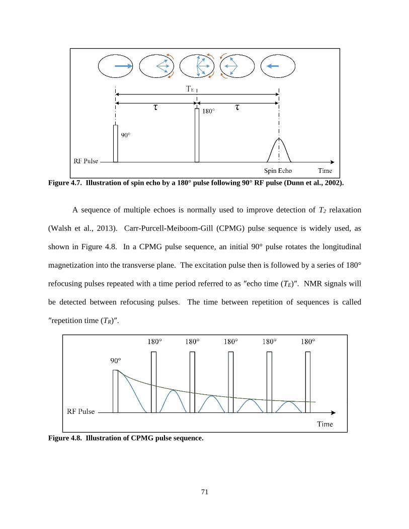
71

Figure 4.7. Illustration of spin echo by a 180° pulse following 90° RF pulse (Dunn et al., 2002).

A sequence of multiple echoes is normally used to improve detection of T2 relaxation

(Walsh et al., 2013). Carr-Purcell-Meiboom-Gill (CPMG) pulse sequence is widely used, as

shown in Figure 4.8. In a CPMG pulse sequence, an initial 90° pulse rotates the longitudinal

magnetization into the transverse plane. The excitation pulse then is followed by a series of 180°

refocusing pulses repeated with a time period referred to as ″echo time (TE)″. NMR signals will

be detected between refocusing pulses. The time between repetition of sequences is called

″repetition time (TR)″.

Figure 4.8. Illustration of CPMG pulse sequence.

72

4.2.1.5. Pulsed Field Gradient

Linear variation of the magnetic field across the sample space causes the Larmor

frequency associated with the nucleus to vary by position. This intentional variation in Larmor

frequency is the basis for spatial resolution of proton density and magnetic resonance imaging

(MRI). This linear variation of magnetic field is applied as a pulse by an independent coil

(Callaghan 1991). Therefore, local Larmor frequency through the sample space is described by

the following equation:

GrBr o )( (4.9)

where G is magnitude of field gradient at position r, parallel to B0.

4.2.1.6. Relaxation Mechanism of Fluids in Porous Media

Three mechanisms are involved in measured relaxation times (T1 and T2) of fluids in

porous media, indicated in following equations (Walsh et al., 2013; Ellis and Singer 2007;

Coates et al., 1999):

surfacebulk TTT 111

111 (4.10)

diffusionsurfacebulk TTTT 2222

1111 (4.11)

where T1bulk and T2bulk are the respective relaxation times of bulk pore fluid. T1surface and T2surface

are the relaxation times of pore fluid due to the effect of porous media grains surface. T2diffusion is

the transverse relaxation time of pore fluid induced by diffusion in the magnetic field gradient.

The relative importance of the three relaxation mechanisms (i.e., bulk, surface, and diffusion)

depends on the physicochemical properties of fluid, size of the pores, pore size distribution,

surface area of the porous media, surface mineralogy of grains, magnetic field gradient, etc.

(Walsh et al., 2012; Ellis and Singer 2007; Coates et al., 1999).

73

4.2.2. Literature Review

NMR studies of porous media and pore fluids started in the 1950s in the oil industry

(Kleinberg and Jackson 2001). For many decades, magnetic resonance relaxometry has been

employed to discriminate oil and oil-products from water in porous media, referred to as ″fluid

typing″. Generally, fluid typing is based on the measurement and interpretation of observed

contrasts in relaxation times (T1 and T2) and diffusion coefficient (D) of pore fluids in porous

media (Coates et al., 1999; Chen et al., 2002). Since the relaxation time of pore fluids is a

function of surface relaxation, the feasibility of discrimination of pore fluids is considerably

reduced due to insignificant contrast in detected signals (Chen et al., 2002). Therefore, by

doping one of the pore fluids (normally, water) with a small concentration of paramagnetic ions

(e.g., Cu2+ or Mn2+, Chen et al., 2002; Balcom et al., 1993), the contrast between the relaxation

times of these pore fluids increases significantly.

Rothwell and Vinegar (1985) studied Berea sandstone using an NMR method. They

measured T2 relaxation time to resolve spatial variations of fluid-filled pores and the physical

nature of the pores. The authors proposed that discrimination of oil and water could be

performed based on the contrast in relaxation times (T1 and T2). They concluded that where the

contrast in relaxation times is large, discrimination of water from oil is plausible. However, pore

size distribution and physicochemical properties of pore fluids (e.g., viscosity) govern this

contrast. The authors suggested that if the relaxation time contrast of pore fluids is not

measurable, doping the water with paramagnetic ions can create a contrast. Chen et al. (1988)

studied immiscible-fluid (Soltrol® 100) displacement in porous media by measuring T1 relaxation

time. Ni2+ had to be added to enhance the NMR signals of water. Araujo et al. (1989)

demonstrated how to classify different samples of crude oil using T1 and T2 measurements. The

74

authors indicated that the T1 contrast between different phases was more pronounced in this

study. Davies et al. (1994) studied discrimination of oil and brine on oil-bearing reservoir core

from the North Sea by measuring T1 distribution. For brine saturated core, the T1 distribution

curve showed a unimodal distribution since preserved samples with oil showed a bimodal T1

distribution curve, which was a basis for discrimination of two fluid phases. Chu et al. (2004)

studied NAPL in heterogeneous porous media using NMR. The study employed T1

measurements to discriminate different fluid phases. Also, they used CuSO4 as a paramagnetic

species to enhance the proton signals of water by reducing the T1. However, naturally short-

lived relaxation time distribution of water and oil in porous media could make the use of

paramagnetic ions ineffective (Li et al., 2007). Moreover, using a high concentration of

paramagnetic ions might increase the risk of interaction between the paramagnetic ions and the

porous media (Li et al., 2007).

Although early studies concerning fluid typing were based on measurements of

individual relaxation times, mapping and interpretation of two-dimensional parameters (e.g., (T2,

T1) or (T2, D)) have become a point of interest recently. Sun (2007) employed two-dimensional

nuclear magnetic resonance logging for in situ fluid typing using T2 and D. Due to significant

difference in diffusion coefficients of water and oil, the discrimination of oil from water signal in

a two-dimensional NMR map was more pronounced. Li et al. (2007) explored discrimination of

water and hydrocarbon in porous media by mapping T1, T2, and D. The authors indicated that the

most effective method for discriminating oil from water is diffusion coefficient mapping.

Ranhong and Lizhi (2011) discussed the application T1 and D contrasts to discriminate the fluids.

Also, they interpreted two-dimensional parameters of measured (T2, D) and (T2, T1). They

indicated that the (T2, D) method is more effective in typing oil and water. However,

75

measurement and interpretation of multiple NMR parameters need significant effort, and a robust

scanning method is still lacking.

Pervizpour et al. (1999) studied the application of MRI to hydrocarbon-contaminated

porous media. They scanned columns of glass beads saturated with distilled water and TCE

(volume ratio of 2:1) based on measured relaxation times. The TCE was not distinguishable

from glass beads, since the proton signals of water were dominant due to relatively higher molar

concentrations of water-bound hydrogen atoms (approximately 145 times greater). This issue

remains a key challenge in the use of NMR for fluid discrimination in porous media today.

Overall, attempts to discriminate water from NAPL using NMR methods consists of the

interpretation of the contrasts in relaxation times (T1 and T2), coefficient of diffusion (D), or two-

dimensional mapping of NMR parameters. Given that the NMR parameters are a function of

pore size geometry (i.e., pore size distribution), surface area of the porous media,

physicochemical properties of pore fluids (i.e., viscosity, molar concentration of 1H in

multiphase fluids), and environmental conditions (e.g., temperature and pressure), detection of a

contrast in NMR parameters is not always successful. Therefore, novel methods need to be

developed for this purpose.


The discrimination of pore fluids via NMR, and thus the use of this technology for the

analysis of spatial contaminant distribution and concentration, remains a key challenge. Thus,

the overarching objective of this research is to develop a practical approach that can qualitatively

and quantitatively resolve the NAPL distribution within saturated porous media. Because the

(liquid-state) 1H-NMR can only detect hydrogen within liquid, but not solid phases, the

following hypotheses will be tested:

76

Hypothesis 4: Freezing the water while keeping the NAPL in a liquid state selectively

suppresses the NMR signal of water-bound hydrogen.

Hypothesis 5: The selective freezing of water within porous media enables resolution of

NAPL distribution within the frozen sediment core, both qualitatively and quantitatively (i.e., as

concentration).


qualitatively discriminate LNAPL from water in situ, using short- and long- echo times.

4.4. Methods

This section describes the NMR measurements and imaging methods used to resolve

NAPL distribution in unconsolidated geological formations. The contents include laboratory

experiments to detect distribution of trichloroethylene (TCE, as a DNAPL) within frozen

sediment core. Also, downhole NMR logging measurements were performed at a former

refinery in the western U.S. in an effort to discriminate LNAPL from water qualitatively.

4.4.1. Laboratory Study

Laboratory NMR investigations were set up to test Hypotheses 4 and 5. Fabricated

sediment core of Colorado silica sand (mesh size #20-#50, φ=0.30) saturated with DI water and

TCE (a DNAPL with a melting point of -73 °C) as model contaminant was remolded in a PTFE

liner. The PTFE liner was designed and fabricated to have 2-inch ID and 2-inch length. To keep

the core frozen during the scanning, a hollow Styrofoam cylinder (6-inch OD and 6-inch long)

was developed and used as an insulation and liner holder inside the MRI probe (Figure 4.9).

77

Figure 4.9. PTFE liner and Styrofoam holder: a) cross-section of PTFE liner and components b) Styrofoam as a thermal break and liner holder inside the NMR probe.

Furthermore, a temperature control system was designed and fabricated, as shown in

Figure 4.10. This system functions by delivery of cold nitrogen gas (from a liquid nitrogen

Dewar) into a PVC freezing chamber that holds the PTFE liner. The temperature of the cold

nitrogen gas is controlled by an in-line heater connected to a proportional–integral–

derivative controller (PID controller). The liquid nitrogen Dewar, in-line heater, and PID

controller are set up outside of the MRI room. The delivery line consists of a ¾-inch rubber

vacuum hose, connecting the system to the PVC freezing chamber inside the MRI probe.

The core was scanned by a magnetic resonance scanner at the Rocky Mountain Magnetic

Resonance Center (RMMRC) at CSU. The scanner was a Bruker small-animal scanner 2.3 Tesla

(100 MHz) with a six-inch-diameter probe (Figure 4.11).

78

Figure 4.10. Temperature control system: a) schematic of the system set-up and b) the freezing chamber and sample holder inside the MRI probe.

Figure 4.11. Bruker small-animal MRI scanner with 2.3 Tesla (100 MHz) at RMMRC, CSU.

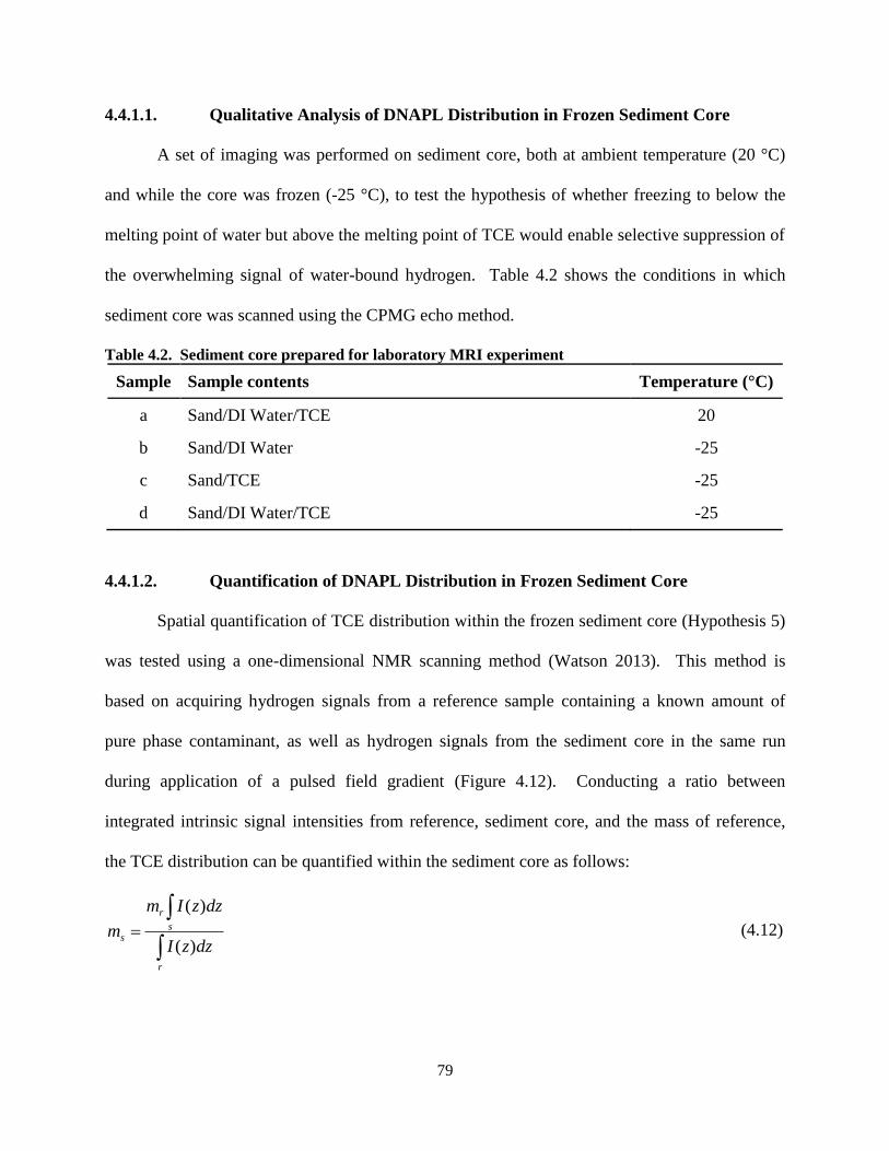
79

4.4.1.1. Qualitative Analysis of DNAPL Distribution in Frozen Sediment Core

A set of imaging was performed on sediment core, both at ambient temperature (20 °C)

and while the core was frozen (-25 °C), to test the hypothesis of whether freezing to below the

melting point of water but above the melting point of TCE would enable selective suppression of

the overwhelming signal of water-bound hydrogen. Table 4.2 shows the conditions in which

sediment core was scanned using the CPMG echo method.

Table 4.2. Sediment core prepared for laboratory MRI experiment

Sample Sample contents Temperature (°C)

a Sand/DI Water/TCE 20

b Sand/DI Water -25

c Sand/TCE -25

d Sand/DI Water/TCE -25

4.4.1.2. Quantification of DNAPL Distribution in Frozen Sediment Core

Spatial quantification of TCE distribution within the frozen sediment core (Hypothesis 5)

was tested using a one-dimensional NMR scanning method (Watson 2013). This method is

based on acquiring hydrogen signals from a reference sample containing a known amount of

pure phase contaminant, as well as hydrogen signals from the sediment core in the same run

during application of a pulsed field gradient (Figure 4.12). Conducting a ratio between

integrated intrinsic signal intensities from reference, sediment core, and the mass of reference,

the TCE distribution can be quantified within the sediment core as follows:

r

s

r

sdzzI

dzzIm

m)(

)( (4.12)

80

where r and s are subscripts for reference sample and sediment core, respectively. I(z) is the

intrinsic signal intensity predicted from detected FIDs, and m is the mass.

Figure 4.12. Schematic of reference and sediment core placed in the MRI probe to quantify TCE distribution using a one-dimensional (along z-axis) NMR scanning method (Watson 2013). In all experiments, field of view (128 mm) is divided to 128 voxels (voxel length = 1 mm).

Because the NMR probe is not able to collect the signal intensity at time zero

(immediately after the RF pulse), the non-parametric regression method was employed to predict

the intrinsic signal intensities within the field of view. In comparison to the least-squares

parametric regression method, which minimizes the sum of the squares of errors, non-parametric

regression uses a continuous function to fit the measured data (Uh and Watson 2014). In this

study, measured NMR signals were analyzed by ParaVision® Bruker software to create images.

However, the detected FIDs were post-processed using the non-parametric regression to predict

intrinsic signal intensities (Uh and Watson 2014). The measured FID of an NMR experiment on

sediment core saturated with TCE at -25 °C was curve-fitted using non-parametric regression as

well as parametric regression methods. In parametric regression, single-, two-, three-, and four-

term exponential functions were tested using MATLAB (using Equation 4.8).

Soil Core

Voxel

Field of View

Reference

MRI Probe

X

Y

Z

81

To quantify TCE distribution within the sediment core, a graphical user interface (GUI)

was developed in MATLAB that automatically analyzes the predicted signal intensities and

provides graphs to visualize contaminant distribution within the sediment core as well as a

tabular data set as the output. To increase the accuracy of TCE quantification within sediment

core, a set of scanning experiments was designed and performed to optimize the method and/or

devices. To eliminate the potential issues associated with circulating nitrogen gas inside the

NMR probe, the temperature control system was removed, and hollow-cylinder Styrofoam was

used as insulation again. The strategy was comprised of the scanning of pure water and pure

TCE in the PTFE liner, fabricated sediment core (fine sand, mesh size #20-#50 and coarse sand,

mesh size #4-#8) saturated with TCE in the PTFE liner, and fabricated glass-beads core (fine

glass beads, 200 to 500 µm and coarse glass beads, 3 mm) saturated with TCE in the PTFE liner.

NMR measurements of the core was performed at -25 °C and 20 °C. Also, various parameters

(i.e., TE and TR) were tested to acquire the best percentage of TCE mass recovery.

4.4.2. Field Study

Downhole NMR logging tools were used at a former refinery in the western U.S. The

former refinery with approximately 200 acres is underlain by North Platte River alluvium.

Sediments grade from sand and silt at ground surface into point bar sands and channel gravel

with depth. The site is impacted by historical releases of petroleum-based hydrocarbons (diesel

and gasoline, LNAPLs) associated with operations between 1923 and 1982. This study was

performed to test Hypothesis 6, that is, whether in situ discrimination of the hydrocarbons (i.e.,

diesel and gasoline) in an LNAPL-contaminated site is possible using downhole NMR logging

tools by imposing short- and long-echo times. Six locations were selected for the experiments,

as shown in Figure 4.13. MLSTE#1, a location showing no contamination and thus serving as

82

control, is located north of the river. However, the remaining five locations are within the

impacted zone.

Figure 4.13. Locations of downhole NMR experiment at a former refinery in the western U.S.

Javelin downhole NMR logging tools (Vista Clara, Inc.) were used in this study. The

tools were comprised of a surface station, a cable winch, a laptop, Javelin software as interface, a

power generator to produce electrical power for the system, a noise reference box to detect noise

at surface, a tripod, and a downhole probe (Figure 4.14). Specifications of the Vista Clara

downhole NMR probes are described in Table 4.3.

83

Figure 4.14. Vista Clara NMR logging tools a) surface station, winch, and laptop, b) tripod, and c) downhole NMR probe.

A JP 175 downhole NMR probe with 1.75-inch OD was used in MLSTE#1, #2, and #3.

A JP255 downhole NMR probe was used in SS-45, SS-26d, and SS-115. The CPMG pulse

sequences were applied at frequencies of 245 kHz and 290 kHz to measure the signals at 2 radii

from the center of the probe within the formation. The results of both measurements were

averaged to improve the signal quality. The system works based on measuring T2 relaxation

times of perturbed protons in the formation imposing CPMG pulse sequences.

Table 4.3. Specification of Javelin downhole NMR logging tools used at the former refinery in the western U.S.

Probe Model Vertical

Resolution (m) Diameter of

Sensitive Shell (cm) Probe Outer

Diameter (cm) Probe

Length (m) JP175 1.0 12 4.5 2.1 JP255 1.0 15 6.4 1.5

The first set of experiments was performed at MLSTE#1, #2, #3, and SS-26d to detect

relaxation time distribution of protons within the formation. In these experiments, an echo time

(TE) of 2 milliseconds and repetition time (TR) of 8 seconds were used. The second set of

experiments was performed at SS-45 and SS-115 to discriminate LNAPL and water (i.e., fluid

typing) within the formation. For fluid typing, pulse sequences with short- and long-echo times

84

(echo spacing) ranging from 1.7 milliseconds to 12 milliseconds were imposed at the depth

where LNAPL resided (just above the water table, Figure 4.13). Generally, by applying a short-

echo time, the relaxation of hydrocarbon and water may overlap, and the two constituents cannot

be distinguished in the T2 relaxation time distribution (Figure 4.15). As the echo time is

increased, relaxation becomes dominated by fluid-diffusion effects. Fluids with a higher

diffusion coefficient (D) will undergo a larger shift to shorter T2, while fluids with lower D will

shift less, potentially allowing for separation of the peaks, with the total signals remaining at

long T2, indicating the volume of hydrocarbon (Akkurt et al., 1998; Coates et al., 1999).

Figure 4.15. Fluid typing by interpretation of T2 distribution of multiphase pore fluid in response to short- and long-echo times (Coates et al., 1999).


This section provides results and discussion of the NMR study. The results of laboratory

and field studies are presented and discussed separately in the following sub-sections.

85


4.5.1.1. Qualitative detection of DNAPL within Frozen Sediment Core

Figure 4.16 shows magnetic resonance images of sediment core saturated with DI water,

TCE, and DI water/TCE at room temperature (20 °C), and while the core was frozen

(at -25 °C). The images indicate that in unfrozen sediment core (at 20 °C) saturated with DI

water and TCE (volume ratio 8:2), discrimination between these two liquids was not possible

(Figure 4.16a). This result is likely due to the fact that the strongest NMR signal (appearing as

brightness) stemmed from water-bound hydrogen relative to the hydrogen within the TCE

molecules since the molar concentration of water-bound hydrogen atoms is approximately 292

times greater than the molar concentration of the TCE-bound hydrogen atoms. Therefore, the

samples were frozen at -25 °C to transfer water into the solid phase, while TCE remained in a

liquid state.

Figure 4.16. Images of the scanned sediment core at RMMRC a) sand, DI water, and TCE at 20 ˚C, b) sand and DI water at -25 ̊C, c) sand and TCE at -25 ̊C, and d) sand, DI water, and TCE at -25 ºC. In image (d), the core was placed in the freezer vertically, thus, the TCE sunk and water froze on the top of TCE. However, the core was scanned horizontally.

86

A comparison between Figure 4.16b and Figure 4.16c clearly illustrates that in the frozen

sediment core at -25 °C, the NMR signal of water-bound hydrogen was successfully suppressed

(excluding minimal background noise), while the liquid-state TCE produced a strong, bright

signal. When both water and TCE were present, a much stronger signal was obtained from the

phase-separated TCE (left of the sediment core in Figure 4.16d) than from the frozen water at

-25 °C (right of the sediment core in Figure 4.16d), proving Hypothesis 4 true and illustrating the

great potential of this technique for targeted NAPL detection in frozen sediment core. Therefore,

by freezing the core, the strong NMR signal of water-bound hydrogen was suppressed, enabling

qualitative discrimination and detection of NAPL.

4.5.1.2. Quantification of DNAPL within Frozen Sediment Core

The results of the predicted intrinsic signal intensity using non-parametric and parametric

regression methods are compared in this section. The regressions were performed on selected

voxels within a sediment core saturated with TCE at -25 °C. Figure 4.17 presents residuals of

non-parametric regression and parametric regressions using single-, two-, three-, and four-term

exponential functions. The results in Table 4.4 indicate that the curve fitted on measured FID of

the specific voxel within the sediment core (herein, voxel #50) using the parametric regression

method improved by increasing the number of exponential terms from a single- to four-term

exponential function. Although the coefficient of determination (R2) did not change substantially

by increasing the number of exponential terms, the residual plot (Figure 4.17) shows that non-

parametric regression has minimal errors. Collectively, non-parametric regression provides more

sensitivity to predict intrinsic signal intensities and thus has been used in this study.

87

Figure 4.17. Residuals of non-parametric and parametric regressions to predict intrinsic signal intensities. The measured FID selected from voxel #50 within the core saturated with TCE at -25 °C.

Post-analysis of intrinsic signal intensities acquired from non-parametric regression was

performed using GUI MATLAB to quantify TCE distribution within the frozen sediment core.

Figure 4.18 shows an example of this analysis of data collected from NMR study of a sediment

core saturated with TCE at -25 °C. The figure shows the quantification curve and spectrum, as

well as tabular output data. In this experiment, only 70% of TCE mass within the core was

detected using a one-dimensional NMR scanning method.

Table 4.4. The results of parametric- compared to non-parametric regression Number of exponential

terms R2 Adjusted

R2 RMS Intrinsic intensity

(parametric)

Intrinsic intensity (non-parametric)

1 0.9806 0.9792 2.255e+04 6.226e+05

757028 2 0.9238 0.9125 7.591e+03 7.518e+05 3 0.9967 0.9959 7.591e+03 7.528e+05 4 0.9968 0.9957 7.583e+03 7.546e+05

88

Figure 4.18. MATLAB GUI developed for one-dimensional quantification of NAPL within the sediment core.

As explained in the methods section, a set of NMR experiments were set up to

troubleshoot the source of inconsistency in TCE mass quantification within the sediment core.

The results of troubleshooting of the method and machine are discussed here and are shown in

APPENDIX C (Figure C-1 through Figure C-5). Echo times of 4.9 milliseconds to 30

milliseconds and repetition times of 10 seconds to 30 seconds were selected to improve the

detection of hydrogen signals. With the exception of analysis on pure DI water, analysis of

NMR signals collected from scanning of pure TCE, coarse (mesh size #4-#8) and fine (#20-#50)

Colorado silica sand saturated with TCE, coarse (3mm) and fine (200-500 microns) glass beads

saturated with TCE did not lead to a consistent number in terms of recovery of TCE mass. The

89

results of scanning pure TCE at -25 °C and 20 °C indicated recovery of TCE mass between 73%

to 115% (APPENDIX C, Figure C-1). Scanning of sediment core containing coarse sand

saturated with TCE at -25 °C and 20 °C showed that recovery of TCE mass ranged between 74%

to 91% (APPENDIX C, Figure C-2). Scanning of sediment core containing fine sand saturated

with TCE at -25 °C and 20 °C indicated the recovery of TCE mass between 42% to 85%

(APPENDIX C, Figure C-3). To minimize the effects of grain-size distribution that directly

influences pore size distribution, and consequently the NMR signals (Coates et al., 1999; Ellis

and Singer 2007), spherical glass beads were used. Coarse glass beads saturated with TCE were

placed in the PTFE liner. Scanning of this core indicated 65% to 95% recovery of the TCE mass

(APPENDIX C, Figure C-4). However, the same study using fine glass beads indicated recovery

ranging from 83% to 96% of TCE mass (APPENDIX C, Figure C-5).

To date, various probable factors contributing to the lack of success in the accurate

quantification of TCE within the porous media using a one-dimensional NMR scanning method

have been tested. Hardware factors, including adjustment of DC offset and quad ghost of the

receiver, replacement of the gradient controller, and patching holes of the scanner room did not

make significant changes. Also, software factors, including adjustment of the scanning method

(i.e., varying TE and TR), did not contribute enough to resolve the inconsistency. Collectively, a

comprehensive and fundamental study of a one-dimensional NMR scanning method to quantify

DNAPL distribution in sediment core is suggested for future research to further test Hypothesis

5. Employing proper rock/sediment core scanner (e.g., Magritek NMR core analyzer and

GeoSpec2 core analyzer) are suggested for this purpose. These scanners are designed with

different magnetic-field strength for core size ranging from 1- to 6-inch diameter and can keep

the temperature of the core constant during the scanning time. These scanners are widely used in

90

petrophysics. Also, since the molar concentration of water-bound protons to the molar

concentration of TCE-bound protons is relatively high in most contaminated sediment core (at

least an order of magnitude higher), one potential topic of research is an NMR study of targeted

nuclei associated with the contaminant (e.g., Cl in chlorinated solvents). However, a proper

Chlorine-NMR scanner with minimum 2- to 2 ½-inch probe is needed to fit the sediment core

inside.

4.5.2. Field Study

The results of downhole NMR logging are presented here. The results are discussed to

determine whether in situ discrimination of the hydrocarbons (i.e., diesel and gasoline) is

possible by imposing short- and long-echo times. Figure 4.19 shows the results of NMR logging

to detect NMR signals at MLSTE#1 (background zone) using Javelin JP175. The T2 distribution

and estimated water content versus depth shown in this figure are collected from depths of 3.2 m

to 4.6 m bgs by logging intervals of 0.5 m. In this measurement, considering less than 3% noise,

the NMR signals with sufficient resolution were detected. Since this location was

uncontaminated, all collected NMR signals were acquired from water-bound protons. Clay,

capillary, and immobile water content shown in Figure 4.19b are determined by Vista Clara

software based on applying cut-off times on T2 distribution curves. However, the application of

cut-off times for various geological formations was not modified. Hence, the data shown in

Figure 4.19b are of conceptual nature and may be non-representative.

The measured data of downhole NMR logging at MLSTE#2 by 0.5-m logging intervals

are shown in Figure C-6 of APPENDIX C. At this location, the NMR signals could not be

interpreted with enough resolution. One factor preventing resolution of NMR signals at

MLSTE#2 was approximately 20% to 30% noise, probably stemming from the pumping facility

91

close to the monitoring well or from the power lines passing over the region. At MLSTE#3,

because the water table was at the very bottom of the monitoring well (4 m bgs), a deeper

monitoring well, SS-26d, was studied in the same zone. The measurements were taken from 3.5

m to 13.5 m bgs by 0.5-m logging intervals. NMR signals of hydrogen atoms associated with

both water and LNAPL were detected with sufficient resolution. The level of noise below 8 m

bgs was measured less than 3%. The collected data from SS-26d are presented in Figure C-7 of

APPENDIX C.

Figure 4.19. The results of downhole NMR logging at MLSTE#1: a) T2 distribution versus depth and b) water content versus depth.

The result of fluid typing using a JP255 downhole NMR logging probe at SS-45, at the

depth where LNAPL existed (based on the previous data, approximately at 4.8 m bgs), is shown

in Figure 4.20. The T2 distribution curves did not show bimodal peaks by imposing short-echo

time (1.7 milliseconds) and long-echo time (12 milliseconds), possibly because of a high level of

(a) (b)

92

noise in this location. Therefore, the data quality is insufficient for conclusive determination and

discrimination of LNAPL from water. At monitoring well SS-115, the same issue prevented

detection and discrimination of LNAPL and water, as is shown in Figure C-8 of APPENDIX C.

The source of noise at both locations could stem from the power lines passing over the region or

active facilities in the site.

Figure 4.20. Measured NMR logging data at SS-45 from a) short- and b) long-echo times.

Collectively, application of low-frequency downhole NMR logging tools at the LNAPL-

contaminated site was sensitive to the noise, type of formation, and saturation of the formation.

The results indicated that increase in level of noise can compromise detection of NMR signals.

The source of noise in this site could stem from the active facilities close to the monitoring wells

or from the power lines passing over the region. Also, existence of fine grain materials can

restrict the movement and relaxation of hydrogen atoms (Coates et al., 1999; Ellis and Singer

2007). On the other hand, estimation of proton density and fluid content using NMR signals is

established on the assumption that the formation is fully saturated. Therefore, in the unsaturated

zones, this method needs to be modified considering the degree of saturation. A low magnetic

field of the downhole probe can also be a factor contributing to the lack of success in this study.

93

A low magnetic field does not provide sufficient polarization and net magnetization. To

complete the testing of Hypothesis 6, a more controlled study at a pilot scale in the laboratory is

needed to develop downhole NMR logging tools and methods, in particular for in situ fluid

typing.


Both laboratory- and field-scale investigations were carried out in this study to test the

viability of NMR for the qualitative and quantitative analysis of NAPL in unconsolidated

geological formations. A laboratory study was performed to verify whether freezing the

sediment core suppresses the overwhelming NMR signal of water-bound hydrogen atoms and

consequently enables targeted resolution of NAPL distribution within the porous media.

Fabricated sediment core of 2-inch diameter and 2-inch long, consisting of Colorado silica sand

(mesh size #20-#50) saturated with DI water and TCE was scanned and imaged at 20 °C and -25

°C. The acquired images revealed that freezing the water indeed selectively suppressed the

NMR signals of water-bound protons. However, since the TCE was still in its liquid state

(melting point of -73 °C), the NMR signals of TCE-bound hydrogen atoms were detectable.

Therefore, freezing the porous media is an alternative to discriminate water from NAPL such as

TCE, using NMR method.

Furthermore, quantification of TCE mass distribution within the frozen core using NMR

measurements was evaluated. A one-dimensional NMR scanning method (Watson 2013) was

used for this study. The intrinsic signal intensities of NMR measurements were determined

using a non-parametric regression method (Uh and Watson 2014). Comparison between the non-

parametric regression and the parametric regression on an NMR study of a frozen core saturated

with TCE (at -25 °C) indicated advantages for the non-parametric method. A GUI MATLAB

94

was developed for quantification of TCE within the sediment core using NMR measurement

data. However, poor accuracy in the quantification of TCE mass within the sediment core was

observed. A series of troubleshooting experiments were performed on pure TCE, indicating that

the inaccuracies were caused by effects of grain-size distribution that directly influences the

pore-size distribution and consequently the NMR signals, as well as potentially by hardware

limitations. Further research is needed to increase the accuracy of NAPL quantification within

porous media.

Finally, downhole NMR logging of an LNAPL-contaminated site was studied at a former

refinery in the western U.S. to test whether in situ discrimination of hydrocarbons is possible by

imposing short- and long-echo time. Monitoring wells with PVC casing were logged at a

background (clean) zone, as well as impacted zone, using Javelin NMR tools (Vista Clara, Inc.).

NMR logging of MLSTE#1 at the background zone indicated detection of water below the water

table with the level of noise as high as 3%. The level of noise at MLSTE#2 (impacted zone) was

high (20-30%), so NMR signals were not detectable. The source of noise possibly stemmed

from the pumping facility’s proximity to the monitoring well or from the power lines passing

over the region. NMR logging of MLSTE#3 at the impacted zone was not successful due to the

low level of the water table (about 8 m bgs). Therefore, a deeper monitoring well (SS-26d) was

studied. NMR logging of SS-26d indicated sufficient resolution below the water table (8 m bgs).

Discrimination of water and LNAPL using downhole NMR logging tools was tested at

two monitoring wells (SS-45 and SS-115). Application of short- and long-echo time, which is

normally used in fluid typing in terms of acquiring bimodal T2 distribution, was not successful

due to the high level of noise stemming from the active facilities in the vicinity of the study area

or from the power lines passing over the region. Potential factors leading to failure of in situ

95

discrimination of LNAPL using downhole NMR logging tools were high level of noise and

probably existence of fine grain materials. Also, low magnetic field of downhole probe could be

a factor contributing the lack of success in this study. Herein, a more controlled study is needed

to develop downhole NMR logging tools and methods to detect and discriminate LNAPL in the

formation.

Consequently, this study shows that freezing the sediment core for the discrimination of

NAPL from water is a promising approach to overcome currently existing technology gaps

outlined in the literature review section. There are, however, potential limitations in freezing the

core that should be taken into consideration for future development. First, the NMR signals of

soluble contaminants in water phase (i.e., aqueous phase) may also be suppressed by freezing the

water. Secondly, freezing the water can change the pore geometry of the porous media and thus

compromise the NMR response by the pore fluid that is still in liquid phase. Thirdly, the effect

of temperature on detected NMR signals of liquid phase pore fluid remains to be studied (Coates

et al., 1999; Ellis and Singer 2007).

The use of a rock/sediment core scanner (e.g., Magritek NMR core analyzer and

GeoSpec2 core analyzer) is suggested since these types of scanners are designed to study pore

geometry as well as pore fluids of porous media (Keating 2014). These rock core scanners are

able to control the temperature of the core during the scanning time. Also, due to a high molar

concentration of water-bound hydrogen relative to the molar concentration of TCE-bound

hydrogen, NMR study of targeted nuclei associated with the contaminant (e.g., Cl in chlorinated

solvents) is proposed using a suitable Chlorine-NMR scanner.

In conclusion, if future research addresses the remaining limitations regarding

quantification inaccuracies, this novel approach is a promising alternative to the conventional

96

laboratory analysis (e.g., via solid-liquid extraction followed by chromatographic analysis),

simplifying sample processing since sediment core is often shipped frozen from the field to the

analytical laboratory. Increasing workplace safety by minimizing contaminant volatilization is

an added benefit. Furthermore, since NMR detects hydrogen atoms in liquid-state fluids, this

approach can be expanded to include the analysis of other H-containing NAPL, such as

petroleum hydrocarbons or nitroaromatic compounds. And although time-consuming, even 3-

dimensional visualization and quantification of NAPL in porous media is possible. This detailed

revelation of contaminant distribution has the potential to lower remediation cost by improving

site conceptual models and enabling smarter and more targeted remediation measures.

97

CHAPTER 5

MONITORING DEPLETION OF LIGHT NON-AQUEOUS PHASE LIQUID IN SHALLOW

GEOLOGICAL FORMATIONS USING ELECTRICAL RESISTIVITY

Co-authors: Maria Irianni Renno, Jens Blotevogel, Thomas Sale


Monitoring contaminated sites before, during, and after remediation is essential to track

the performance of remedies and natural attenuation processes. Historically, monitoring of

contaminated sites has relied primarily on data from monitoring wells and grab sediment

samples. Also, near surface geophysics (e.g., electrical resistivity method, nuclear magnetic

resonance, CT scan, ultrasound, etc.) has been studied to characterize and monitor contaminated

geological media. However, inability to correlate the detected geophysical signals to the

subsurface processes created the demand for better tools to track the efficacy of remedies. In this

study, a vertical resistivity profiling method, as a non-destructive, near-surface geophysical

method, is evaluated to track depletion of light non-aqueous phase liquid (LNAPL) in shallow

geological formation at an LNAPL-contaminated site. A laboratory-scale study indicates that

electrical resistivity profiling is able to resolve depletion of MTBE (an LNAPL) in sand columns

over a period of one month. In this experiment, the primary loss process was volatilization.

Field-scale study of complex resistivity profiling at a former refinery in the western U.S. (an

LNAPL-contaminated site) explores changes in resistivity of the contaminated zone over a

period of one year. Also, water quality (including pH, major ions, sulfate, and TDS) and

temperature were profiled through depths where the complex resistivity was measured. Attempts

to correlate the change in resistivity to water quality and temperature indicated that the resistivity

98

of porous media varies with the concentration of major ions, TDS, and temperature. However,

the resistance to electrical current in an aged LNAPL-contaminated site is controlled by multiple

conflicting factors including hydrogeological and biogeochemical processes. Due to multiple

factors, it appears that tracking remaining LNAPL at field site is at best difficult, and potentially

infeasible, using the electrical resistivity method.

5.2. Introduction

Monitoring contaminated sites before, during, and after remediation is essential to

understanding the efficacy of active remedial measures. Over the past decades, 1G and 2G

characterization methods have been the primary means to monitor remediation systems. Both

strategies are limited with respect to tracking the mass of contamination remaining at a site

through time. Limitations of both 1G and 2G tools and methods are discussed in Sale et al.

(2013 and 2015) and Chapter 1 of this dissertation. The vertical resistivity profiling, as a non-

destructive geophysical method, is an alternative to conventional monitoring methods. This

section explores the capability of in situ vertical electrical resistivity profiling to track vertical

extent and depletion of LNAPL in shallow geological media over time. The following

introduction presents a theoretical basis for the study, literature review, research objective and

research hypothesis.

5.2.1. Electrical Resistivity Method

In this section, the basic principles of electrical resistivity, electrical conductance in

porous media, current flow in porous media, and geometric factor and electrode configurations

are introduced. Based on the reviewed literature, electrical resistivity and electrical conductivity

are reciprocal and, therefore, are interchangeably used in the following text.

99

5.2.1.1. Basic Principles of Electrical Resistivity

The electrical resistivity of a material is the resistance between the opposite faces of a

cube of the material against conducting electrical current (Kearey 2009). Considering a known

electrical current passing through the cube (with known dimensions), the material resists the

conduction of the current, and a potential drop between opposite faces of the cube is measurable

(Reynolds 2011, Figure 5.1). This resistance is directly proportional to the length of the cube

and inversely proportional to the cross-section area of the cube. Resistivity is the constant of this

proportionality (Reynolds 2011):

Figure 5.1. Basic definition of electrical resistivity (Reynolds 2011).

IV

R (5.1)

A

LR (5.2)

A

LR (5.3)

where R is resistance (Ohm, Ω), V is potential difference (volt, V), I is current (ampere, A), L is

the length of cube (meter, m), A is the cross-sectional area of the cube perpendicular to the

current (m2), and ρ is resistivity (Ω∙m). By substitution and rearrangement of Equations 5.1 and

5.3, resistivity is equal to:

100

LA

IV (5.4)

To measure the resistivity of porous media, both direct current (DC) and alternating

current (AC) can be employed. However, in materials with capacitive properties (e.g., saturated

porous media), DC resistivity could be a potential factor affecting polarization of pore fluids.

Therefore, measuring the resistivity of porous media using AC is an alternative to DC resistivity

measurements. However, the capacitive property of saturated porous media causes a phase shift

between the current and the potential which is measurable. The sensitivity of the complex

resistivity measurements to changes in bio-physicochemical properties of porous media has been

investigated by researchers (e.g., Abdel Aal et al., 2004; 2006; and 2014; Davis et al., 2006).

For complex resistivity (or complex conductivity) methods, the measured resistivity and

phase shift between current and potential difference can be converted to real and imaginary

components, as shown in Figure 5.2 and Equations 5.5 through 5.7.

Figure 5.2. Complex resistivity components

22 (5.5)

101

1tan , 73.5 (5.6)

where ρ is the measured resistivity, ρʹ is the real component, ρ″ is the imaginary component, and

ϕ is the phase shift (degrees) of complex resistivity. The real and imaginary components of

complex resistivity are determined by:

cos|| and sin|| (5.7)

5.2.1.2. Electrical Conductance in Porous Media

Electric current may be propagated in porous media in three ways (Reynolds 2011): 1)

electronic (Ohmic) conduction, 2) electrolytic conduction, and 3) dielectric conduction. In

electronic conduction, current flows in materials containing free electrons, such as metals. The

slow movement of ions within an electrolyte that depends on the type of ions, ionic

concentration, and mobility is the source of electrolytic conduction. And, alternating current in

weak conductive materials (or insulators) causes dielectric conduction by shifting atomic

electrons slightly with respect to their nuclei (Reynolds 2011).

In most cases, electrolytes in pore fluids are the primary factor conducting current

through the porous media and rocks. Current flow due to conduction through soil solids is

generally negligible. At the frequencies used in electrical resistivity measurements (less than

1000 Hz), dielectric conduction can be disregarded (Kearey 2009; Reynolds 2011). Equation 5.4

refers to electronic conduction of homogenous material. Equation 5.4 can be applied to

determine the apparent resistivity of a fluid-filled porous medium. Building on these themes,

Archi (1942) developed an empirical equation for apparent resistivity of porous media that

considers porosity, degree of saturation, and resistivity of pore fluid:

fnmSa (5.8)

102

where φ is the porosity, S is the degree of saturation, ρf is the resistivity of pore fluid, a is a

dimensionless parameter related to grain shape, m is a dimensionless parameter related to

cementation, and n is the saturation exponent.

The electrical resistivity of saturated porous media also depends on temperature. Mc Neil

(1980) indicated that the temperature dependence of electrical conductivity is approximately

linear over ambient temperature and could be estimated using:

)25(1)25()( TCT (5.9)

where T is the temperature (°C) at which conductivity or resistivity is measured. The coefficient

is 2.2x10-2/°C which is applicable for most of the ions involved in the electrolytic conduction

of saturated porous media.

5.2.1.3. Current Flow in Porous Media

By imposing an electrical potential in a homogenous medium, a current propagates

radially in a spherical shape (Figure 5.3). The voltage drop between any two points of a sphere

can be described as (Reynolds 2011):

Voltage drop = r

V

(5.11)

The negative sign shows potential decreases in the direction of current flow. Similar to

the flow net of water in porous media, lines of equal voltage (equipotential) and lines of current

are perpendicular (Reynolds 2011).

The current density is the current divided by the area in which the current is distributed

over (for spheres, A=4πr2). To determine the voltage at distance r from the current point source

(Reynolds 2011):

24 r

IJ

r

V

(5.12)

103

Therefore, the voltage at a distance r from the source is:

rI

rrI

VVr

144 2

(5.13)

Vr approaches zero since r→0.

Figure 5.3. Current flow in porous media a) equipotential shell around a point source on a homogenous medium b) potential drop versus distance from the source (Reynolds 2011).

5.2.1.4. Geometric Factor and Electrode Configurations

Apparent resistivity is also a function of electrode array geometry. The effect of

electrode array on resistivity measurements, known as ″geometric factor (G)″, is based on the

fact that the potential Vp at any point P in the ground is equal to the sum of the voltages from the

two electrodes (Figure 5.4):

104

Figure 5.4. Generalized form of the four-electrode configuration in resistivity surveys (Reynolds 2011).

BAp VVV (5.14)

where VA and VB are the potential contributions from two electrodes, A and B. The potential at

electrodes M and N are (Reynolds 2011):

MBAM

IVM

114

(5.15)

NBAN

IVN

114

(5.16)

Potential difference between the two points is:

NBANMBAMI

VVV NMMN

11114

(5.17)

By rearranging Equation (4.16), ρ is:

111114

NBANMBAMIVMN (5.18)

RGGI

VMN (5.19)

Equation 5.19 is the basic equation for calculating the apparent resistivity for any

electrode configuration. Szalai & Szarka (2008) indicated that nearly one hundred different

arrays have been described in the literature.

105

Al though many arrays are used in specific surveys, only a few of them are in common

use (Kearey 2009). Generally, common arrays are categorized into two main groups: 1) two-

electrode array and 2) four-electrode array. The four-electrode array emerged after Wenner

(1915) argued that the resistance between electrodes and the sediment in a two-electrode array is

higher and is not stable. However, the literature considers the two-electrode array as a standard

configuration for downhole well-logging (Milsom and Eriksen 2011).

5.2.2. Literature Review

Historically, more sites are contaminated by petroleum hydrocarbons (i.e., LNAPL) in

comparison with the other types of contaminants in the U.S. (Atekwana and Atekwana 2010).

Generally, LNAPL-contaminated sites are considered to be a dynamic and complex environment

due to physical, chemical, and biological processes. The geoelectrical response of LNAPL-

contaminated sites depends on many factors. Atekwana and Atekwana (2010) categorized main

factors including the type of LNAPL, LNAPL release source, distribution of LNAPL in saturated

and vadose zones, the saturation history of the contaminated media, biological processes, etc.

Atekwana and Atekwana (2010), based on a conceptual model of Sauck (2000), showed a typical

distribution of LNAPL in the shallow subsurface at an early stage during or shortly (weeks to

several years) after the spill (Figure 5.5). The conceptual model of LNAPL distribution in the

subsurface proposed by Sauck (2000) has been summarized by de Castro and Branco (2003) in

Table 5.1.

106

Figure 5.5. Conceptual model of LNAPL distribution at a shallow subsurface (Atekwana and Atekwana 2010).

The saturation history and biological processes of the contaminated zone are the most

important factors affecting the geophysical response of an LNAPL-contaminated site (Atekwana

and Atekwana 2010). Therefore, the behavior of LNAPL-contaminated sites has been

categorized into two stages (Atekwana and Atekwana 2010): 1) a short-term stage that refers to a

time frame of weeks to several years in which chemical and biological alteration of LNAPL in

the contaminated zone is negligible, and only the physical separation of the LNAPL into the

different phases has occurred and 2) a long-term stage that refers to several years to decades

when physical, chemical, and biological properties of the site are altered.

5.2.2.1. Short-Term Geoelectrical Response of LNAPL-Contaminated Sites

Early laboratory research indicated a high resistivity at LNAPL-contaminated zones

(referred to as ″the insulating layer model″ in the literature) compared to background zones due

to the partial replacement of conductive pore water by the highly resistive petroleum compounds

(Olhoeft 1992; Schneider and Greenhouse 1992; Daniels et al., 1992; de Ryck et al., 1993;

107

Endres and Redman 1993; Monier-Williams 1995; Endres and Greenhouse 1996; de Castro and

Branco 2003; Yang et al., 2007). The geophysical response of LNAPL-contaminated zones over

a short period of time is strongly controlled by the physical properties of the LNAPL (Atekwana

and Atekwana 2010). This result is true while the hydrocarbon has not been physically or

chemically altered (Atekwana et al., 2004a).

Table 5.1. Sauk (2000) conceptual model of LNAPL distribution in the subsurface (de Castro and Branco 2003)

Location Hydrocarbon product Vadose zone directly beneath the spill Residual and vapor phases Vadose zone directly above the water table Free (mobile) and residual phases Vadose zone directly above the free/residual LNAPL

Vapor and residual phases

Reactive fringe around the dissolved plume Dissolved phase Anaerobic core of the dissolved plume Dissolved phase Distal end of the dissolved plume Dissolved phase

5.2.2.2. Long-Term Geoelectrical Response of LNAPL-Contaminated Sites

Most field-scale electrical resistivity (or conductivity which is reciprocal of resistivity)

measurements disagree with the results of controlled laboratory studies that used fresh

hydrocarbon products. For instance, high apparent conductivities in LNAPL-contaminated zones

was reported by Monier-Williams (1995). Benson and Mutsoe (1996) and Sauck et al. (1998)

reported low apparent resistivities associated with hydrocarbon-contaminated zones. Bermejo et

al. (1997) reported low resistivities in residual product fuel plumes at Wurtsmith Air Force Base,

Michigan. Atekwana et al. (1988) reported high conductivity at LNAPL-contaminated zones at

Crystal Refinery in Carson City, Michigan. Sauck et al. (1998) hypothesized that geoelectrical

response of LNAPL-contaminated site changes from electrically resistive to a more conductive

behavior with time due to complex biogeochemical processes. Later, Sauck (2000) supported his

hypothesis by proposing a model to show resistivity structure of LNAPL plumes as a dynamic

108

system. The decrease in apparent resistivity was hypothesized due to high conductivity of pore

fluid. This decrease was related to the high total dissolved solids (TDS) in groundwater, a result

of enhanced mineral weathering accompanying the production of carbonic and organic acids

during biodegradation. This model called ″the high conductive layer″ was in contradictory to the

insulating layer model, which assumed that the presence of LNAPL in the subsurface could

increase resistivity in early stages. The study of the LNAPL-contaminated site at Crystal

Refinery by Atekwana et al. (2000) indicated that LNAPL-contaminated zone is a dynamic

system, and therefore, properties of the zone can change over time and position. The study

indicated that the knowledge of geology, geochemistry, and biology of this dynamic and

complex system can lead to a better understanding of subsurface conditions.

Cassidy et al. (2001) indicated a dramatic increase in conductivity due to LNAPL

biodegradation under aerobic and anaerobic conditions that caused a change in pore water

biogeochemistry. Werkema et al. (2002) suggested a possible relationship between the

biodegradation of the LNAPL-contaminated zone and the measured low resistivity. They

provided evidence of high-hydrocarbon degrading bacteria populations in zones where the low

apparent resistivity was measured at Crystal Refinery. The findings of Werkema et al. (2003)

confirmed the high conductive layer model and indicated that biological activities impact the

geophysical properties of LNAPL-contaminated sites. They also suggested that the vertical

position of the high conductivity anomaly occurs in partially water saturated conditions above

the water table. In a mesoscale experiment, Atekwana et al. (2003) showed that dissolved ions in

pore water were higher in diesel-contaminated sediment columns compared to the background.

They provided additional information that the zones with high apparent conductivity associate

with high population degrading microbes.

109

Atekwana et al. (2004a) studied the Crystal Refinery to investigate the effects of

biodegradation processes on the geoelectrical properties of LNAPL-impacted sites. The results

showed a higher apparent conductivity associated with the higher percentage of hydrocarbon

degrading microbial populations. In another study at Crystal Refinery, Atekwana et al. (2004b)

measured the vertical distribution of apparent conductivity and TDS and specific conductance of

groundwater. The results indicated that TDS and apparent conductivity of sediments were higher

at locations contaminated with LNAPL and are undergoing intrinsic biodegradation compared to

the background. This observation was consistent with the conductive layer model.

Atekwana et al. (2004c) studied apparent electrical conductivity of sediments during

microbial mineralization of diesel in a mesoscale laboratory experiment. The temporal elevated

apparent conductivity, dissolved inorganic carbon, and calcium in contaminated columns

suggested that the high apparent conductivity is due to enhanced mineral weathering from

microbial activity. The maximum change in apparent conductivity occurred in the sediments

above the water table that was saturated with diesel.

Abdel Aal et al. (2004), showed that changes in electrical properties of diesel-impacted

sediments were associated with an increase in hydrocarbon degrading microbial population, a

decrease in diesel concentration and terminal electron acceptors (TEAs, e.g., NO3- and SO4

2-,

iron, and manganese), and an increase in Ca2+ from mineral weathering. Atekwana et al. (2004d)

investigated the relationship between TEAs and geophysical properties at a hydrocarbon-

contaminated aquifer. The data showed that higher apparent conductivity overlapped with

discrete zones of TEAs associated with the higher microbial activity.

Atekwana et al. (2005) used the geochemical and stable carbon isotope data of Crystal

Refinery to assess the relationship between biodegradation, mineral weathering, and enhanced

110

apparent conductivity zones. The results showed that the zone with a higher apparent electrical

conductivity in the contaminated aquifer had a higher TDS in comparison to the background.

The higher TDS in contaminated groundwater was due to elevated ion concentrations from

enhanced mineral weathering. The zones with higher TDS overlapped with zones with higher

total petroleum hydrocarbons (TPH), which were the same zones where reduction of nitrate, iron,

manganese, sulfate, and methanogens was occurring. They concluded that the zones of higher

apparent conductivity might be explained by mineral weathering related to hydrocarbon

biodegradation.

Davis et al. (2006) studied the effect of microbial growth and biofilm formation of diesel-

impacted sand columns using complex conductivity measurements. They suggested that the

growth and attachment of microbial cells and biofilms to sand surfaces creates dynamic changes

in the component of complex conductivity (imaginary component). Allen et al. (2007) studied

the relationship between the microbial community structure in LNAPL-contaminated sediments

and geoelectrical signatures at Crystal Refinery. The analysis showed that the increase in

electrical conductivity detected in the free phase LNAPL zone is attributable to the activities of

microbial populations, which possibly alter both the electrolytic properties of the pore fluid and

the interfacial properties of the sediment grains under the anaerobic conditions.

The importance of biological activities in the alteration of the geophysical properties of

LNAPL-contaminated sites led Atekwana et al. (2006) to introduce ″biogeophysics″ as a

multidisciplinary field that is concerned with the geophysical signature of microbial interactions

with geological media. Atekwana and Atekwana (2010) reviewed geophysical signature of

microbial activity at hydrocarbon-contaminated sites. They indicated that changes in rock

properties due to microbial activity has significant impact in shallow depths (<100 m), where

111

biological processes are most active. They also noticed that the excess organic carbon of

LNAPL stimulates microbial activity and thus leads to significant alteration of the

physicochemical properties of contaminated zone. Atekwana and Atekwana (2010) found that

maximum change is in the transition, capillary, and upper portion of the saturation zones. The

highest populations of hydrocarbon degrading microorganisms within these zones cause the

maximum changes in geophysical properties of the subsurface.

Mewafy et al. (2013) investigated the complex conductivity signatures of sediment core

collected from an LNAPL-contaminated site, undergoing biodegradation, near Bemidji,

Minnesota. The results showed that the magnitude of the components of the complex

conductivity (i.e., both real and imaginary) was higher for most of the samples from the zone

where the LNAPL saturation was greatest compared to the plume. Enhanced complex

conductivity responses were associated with zones of high concentration of dissolved Fe2+

resulting from the microbial activities. Abdel Aal and Atekwana (2014) conducted laboratory

experiments to investigate the complex conductivity response of biodegraded hydrocarbon in

porous media. The results indicated an enhancement in conductivity of the porous media due to

biodegradation of hydrocarbon compared to fresh hydrocarbon.

Overall, the short-term geoelectrical response of LNAPL-contaminated porous media is

related to partial replacement of conductive pore water by highly resistive petroleum compounds,

since the long-term geoelectrical response of porous media is a function of many competing

factors. To date, attempts to investigate the long-term geoelectrical response of contaminated

porous media have been done using DC resistivity measurements in both laboratory and field

scale. Also, complex resistivity studies have been performed on a laboratory scale to investigate

sensitivity of this method to the long-term geoelectrical variation of porous media due to

112

biodegradation of contaminants. However, neither one tested the geoelectrical response of

porous media using complex resistivity method in an actual LNAPL-contaminated field site.


Although the electrical resistivity method has been studied in contaminant hydrology for

decades, application of this method to monitor LNAPL impacted-sites still needs more

investigation. The overarching objective of this study is to apply a vertical resistivity profiling

method at an LNAPL-contaminated site to track depletion of LNAPL over time in shallow

geological media. In this study, the following hypothesis is tested:



5.4. Methods

Laboratory and field study using electrical resistivity profiling were performed to track

the depletion of LNAPL over time in unconsolidated porous media. The following section

describes a short-term laboratory study and a field-scale experiment at an aged LNAPL-

contaminated site.


A controlled laboratory-scale experiment was set up to evaluate the electrical response of

unconsolidated porous media to LNAPL depletion over a 30-day period. This experiment was

set up to provide an insight into the electrical resistivity method for short-term where

contaminant has not been involved in significant biogeochemical changes. Colorado silica sand

(mesh size #10 to #20, φ=0.3) was used as porous media. Methyl tert-butyl ether (MTBE, an

LNAPL) was selected as a volatile contaminant (Henry's law constant, H=0.015, Fischer et al.,

2004) to depict LNAPL depletion in a short-term stage. The laboratory experiment was

113

conducted using two sand columns with a multilevel electrode system (MES). Each system had

10 equally-spaced electrodes (three inches from center to center of the electrodes) installed at the

center of the sand column. One column was equipped with water sampler ports at the positions

where the electrodes were installed (Figure 5.6). The electrodes were made of titanium mesh

coated with mixed-metal oxide (ElgardTM 300 anode ribbon mesh), which is dimensionally

stable as anode and cathode material. The titanium mesh was hydrophilic and oleophobic, both

properties allowing the electrode to be wetted by water rather than the LNAPL, preventing a

local high resistive region from forming at the electrode.

The columns (clear acetate pipe, 4-inch OD, and 3-feet long) were packed with sand to ¾

height (~2.5 feet or 75 cm). Both sand columns were saturated with degassed tap water (Fort

Collins, CO) from bottom to top (to minimize air pockets trapped in the sand columns) using a

peristaltic pump at a constant pumping rate of 4.5 mL/min. To have a uniform ion concentration

through the depth of sand columns, the pump was kept running to wash the sand with three pore

volumes (Pv = 1760 cm3 for each sand column). The concentration of ions was analyzed via

high-performance liquid chromatography (Metrohm 838 Advanced Sample Processor) analysis

through water samples taken from the water-sampler ports on one sand column. The sand

columns were contaminated with dyed MTBE (dyed with UVXPBB at 0.1% by mass of MTBE)

from the top of the columns. The MTBE was dyed to enhance visualization of the smeared zone.

Photographic images in Figure 5.7 were acquired using ultraviolet (UV) light.

114

Figure 5.6. Sand columns with a multilevel electrode system (MES) a) before filling with sand b) after filling with sand.

By decreasing the water level to half of the height of the columns' height (between EL4

and EL5; Figure 5.6) and increasing the water level afterward, the top part of the sand columns

was impacted with LNAPL (Figure 5.7). The rate of lowering and raising the water table was

varied between 9 and 4.5 mL/min, respectively.

Figure 5.7. Decreasing and increasing water level to spread out MTBE in sand columns (left to right). The images acquired under UV light.

After increasing the water table to the top of the sand columns, the MTBE pool was

depleted using a syringe. Then, the built-up vapor phase of LNAPL was depleted from the head

space continuously using the capture system shown in Figure 5.8. The capture system includes

an activated carbon cylinder (2-inch OD and 6-inch long PVC pipe), a peristaltic pump, and a

115

water flask. The pump was working continuously to deplete the vapor phase passing through the

activated carbon. The remaining vapor phase was discharged into the water flask.

Figure 5.8. Schematic of the vapor-phase capturing system.

The electrical resistivity of sand columns was measured using the two-electrode array, as

well as the Wenner array (Section 5.2.1.4. ). To measure the resistivity of porous media, AC

currents (12 V and 24 V, 60 Hz) were applied. The data were measured using FLUKE

multimeters (FLUKE 189 True RMS Multimeter). However, the phase was not measured in the

laboratory study. The temperature of the columns was measured through depth at the beginning

and the end of each test using a Micro Temp digital infrared thermometer (MT250).

5.4.2. Field Study

To test whether complex resistivity profiling is capable of tracking depletion of

contaminants over time in an aged LNAPL-contaminated site in heterogeneous conditions, a

field-scale experiment was designed and performed at a former refinery in the western U.S. The

116

site has been contaminated by releases of hydrocarbons (gasoline, diesel, and other motor fuels)

per standard practices of the era of operation for more than 50 years. The geology of the site

consists of fluvial deposits grading from fine to coarse sand with depth. To measure complex

resistivity of the contaminated site through depth, a monitoring system, called ″MLSTE″

(multilevel sampler, thermocouple, and electrode), was designed and installed at two locations

within the site (Figure 5.9): 1) background zone or clean zone at the north property (MLSTE#1)

and 2) impacted zone at the south property (MLSTE#2).

Figure 5.9. Location of MLSTE#1 and MLSTE#2 at the former refinery in the Western U.S.

Each MLSTE had 13 ElgardTM mesh electrodes located at intervals of one foot over a

total length of 13 feet of a 2-inch clear PVC pipe. Water sampler ports (1/8-inch PTFE tubes,

Master FlexTM, Cole Parmer) and thermocouples (type K with 0.5 °C precision) were installed

between the electrodes to extract water samples for water-quality analysis and to measure

temperature, respectively. A 2-inch cap was installed at the end of PVC pipe to avoid intrusion

of water into the pipe after installation. The electrodes were collected in a water-tight box to be

protected. Figure 5.10 shows the MLSTEs before and after installation in the site. At the time of

117

installation, the depth to water at both locations was approximately 8 feet below ground surface

(bgs).

Figure 5.10. The MLSTEs a) before installation, b) water sampler and thermocouple, c) electrode, and d) measuring ports after well completion.

The MLSTEs were installed using a CME hollow stem auger (HSA) drill system with 4-

¼ inch ID auger flights. Below the water table, the formation collapsed around the MLSTE, and

the well was completed by filling the annular space with fine sand (mesh size #20) and the top 2

feet with bentonite (Figure 5.11). Collectively, 13 electrodes and 12 sets of water samplers and

thermocouples were installed at depths of three to 14 feet bgs. During drilling steps, sediment

core was collected using a 1 ½–inch split spoon. Sub-samples were provided at ½-foot intervals,

kept in the bags, and sent to the laboratory on dry ice for geology logging. Logging was

performed by a professional geologist following the guidelines for hydrogeological logging of

samples, presented in Sterret 2007.

118

Figure 5.11. Installation of the MLSTE a) CME drill system with hollow stem auger, b) installing the MLSTE downhole, and c) the MLSTE is covered for protection.

Temporal measurements of electrical resistivity, temperature, and water sampling were

performed for the dates indicated in Table 5.2. The electrical resistivity was measured via two-

electrode array. Complex resistivity measurement was performed using an impedance meter

(LCR meter, BK Precision, model 879B). The temperatures were measured using a handheld

thermometer (TC Direct Digital Thermometer, 305P). The water-table data was collected from

the adjacent monitoring well at both background zone and impacted zones.

Table 5.2. Date of measurements at the former refinery in the western U.S. tn Date of measurement Comment 1 11/06/2013 Complete water quality 2 03/11/2014 Partial water quality 3 05/21/2014 Partial water quality 4 08/14/2014 Partial water quality 5 09/30/2014 Partial water quality

A peristaltic pump (Core Parmer, Chicago, IL) was used to collect water samples. Water

was pumped into a Multi-Probe Flow Monitoring SystemTM to measure pH and ORP (Geotech,

Denver, CO). A Symphony™ pH probe (VWR, Radnor, PA), an oxidation-reduction potential

119

(ORP) probe (model NCL-100, ORION™, ThermoScientific, Waktham, MA), and an ORION™

Five Star Plus meter (ThermoScientific, Waltham, MA) were used to measure pH and ORP of

water, respectively (Irianni Renno et al., 2015).

For cation and anion analysis, water samples were filtered through 0.45-μm Acrodisc™

syringe filters (PSF, Life Sciences Advanced Technologies, St. Petersburg, FL) and collected in

10-ml vials. The latter water samples were preserved by injecting 50 μl of a 70% nitric acid

(HNO3) solution into the sealed vials. More information on water sampling and preservation is

addressed in Irianni Renno et al. (2015). Water samples were placed on ice and transported to

the laboratory. The analysis of hydrocarbons was performed in the laboratory at Colorado State

University (CSU), Fort Collins, CO. The water samples were extracted with high-purity

(>99.0%) hexane (Sigma-Aldrich) and were analyzed via gas chromatography with a flame

ionization detector (FID). Analysis of water samples for ions was performed at the Soil-Water-

Plant Testing Laboratory at CSU (Fort Collins, CO). The type and methods of analysis at the

Soil-Water-Plant Testing Laboratory are summarized in the Table 5.3.

Table 5.3. Standard methods of water analysis at Soil-Water-Plant Testing Laboratory at CSU (Fort Collins, CO)

Parameter Standard Number

Method of Analysis

Anions EPA 300.0 Determination of inorganic anions by ion chromatography

Cations and metals EPA 200.7 Determination of metals and trace elements in water and wastes by inductively coupled plasma-atomic emission spectroscopy

Total dissolved solids (TDS) EPA 160.1 Gravimetric method Conductivity EPA 120.1 Specific Conductance at 25°C


The following section presents the results of the electrical resistivity studies.

Documentation includes the results of laboratory and field experiments.

120


Measured apparent resistivity versus depth for laboratory experiments are shown in

Figure 5.12 and Figure 5.13. The data indicated higher resistivity associated with the presence of

new LNAPL in the smear zone (i.e., the top part of the columns). The resistivity of the smeared

zone decreased over time due to depletion of the LNAPL via volatilization. Use of AC current

avoided polarization of aqueous phase. Resistivity measurements, using 12V and 24V, clearly

indicated the trend of LNAPL depletion over time. There is no evidence of a significant effect of

using 12V versus 24V. Application of the two-electrode array (Figure 5.12) provided a smoother

trend of LNAPL depletion in comparison to the Wenner four-electrode array (Figure 5.13). This

result, contradictory to the literature, might be due to the boundary effect which can be a point of

further research. Collectively, the results of controlled laboratory experiments were in agreement

with the insulation layer model.

Figure 5.12. Measured resistivity versus depth over time by the multilevel electrode system using the two-electrode array and imposing a) AC-12V b) AC-24V.

121

Figure 5.13. Measured resistivity versus depth over time by the multilevel electrode system using the Wenner array and imposing a) AC-12V b) AC-24V.

5.5.2. Field Study

The results of field study are presented in this section. A part of the water-quality data

was lost due to inappropriate storage of collected samples by CSU's Soil-Water-Plant Testing

Laboratory. Figure 5.14 shows the geology logs and apparent resistivity and temperature

profiles of background and impacted zones on the dates indicated in Table 5.2. The geology logs

of both zones show that the sediments generally graded from fine to coarse grain through depth.

The water table data collected from adjacent monitoring wells are also shown in Figure 5.14.

The water table fluctuated between 9.35 and 10.4 feet at background zone and 7.5 and 8.7 feet at

the impacted zone on the dates of measurement. At the background zone, the temperature varied

from about 3 °C to 24 °C at ground surface and from about 9 °C to 14 °C at a depth of 14 feet.

The temperature at the impacted zone varied from about 8 °C to 23 °C at ground surface and

from about 13 °C to 18 °C at a depth of 14 feet. Higher temperature of the deeper zone at the

impacted zone can be associated with heating due to the ongoing sustainable thermally-enhanced

LNAPL attenuation (STELA) project (Akhbari 2013). The main objective of STELA was to

122

keep the temperature of impacted zone above 18 °C to enhance microbial activity and

consequentially natural loss of LNAPL (Zeman et al., 2014).

At the background zone, measured apparent resistivity had values between 29,000 to

280,000 Ω∙m at 3 feet bgs, and a peak with values ranging between 39,000 to 580,000 Ω∙m at a

depth of 5 feet bgs. Apparent resistivity then decreased at the depth of 11 feet bgs and ranged

between 137 to 530 Ω∙m from 11 feet to 14 feet bgs. Between 11 feet to 14 feet bgs, the

variation of apparent resistivity was not significant. The maximum and minimum values of

apparent resistivity through depth over the time are corresponding to the minimum and

maximum level of the water table on September 30, 2014 (8.8 feet bgs) and March 11, 2014

(10.4 feet bgs). The measured phase varied from 0.84 to 1.34 degrees at 3 feet bgs, a peak with

values ranging from 2.9 to 4.57 degrees at the depth of 6 feet bgs, and values ranging from about

0.4 to 1.0 degrees between depths of 7 and 14 feet bgs.

123

Figure 5.14. Collected data from background and impacted zones: a) geology logs, b) apparent resistivity, c) measured phase d)

real component, e) imaginary component, and f) measured temperature.

124

The trend for calculated real and imaginary components of apparent resistivity was the

same as measured apparent resistivity through the depth over time. However, the imaginary

component indicated more sensitivity, as shown in Figure 5.14. Based on Archie's law, high

values of apparent resistivity above the water table (AWT) are associated with the degree of

saturation less than 100%. Therefore, low values of apparent resistivity were measure below the

water table.

At the impacted zone, the highest values of apparent resistivity were measured at the

depth of 3 feet ranging from 5,300 to 31,000 Ω∙m. Apparent resistivity decreased versus depth

and ranged from 221 to 1336 Ω∙m at a depth of 14 feet over time. The highest values of the

phase were measured at depths between 6 and 8 feet bgs. This observation corresponded to the

water tables varying between 7.5 and 8.8 feet bgs. A peak in phase was measured at a depth of 7

feet bgs with the values ranging from 2.3 to 3.4 degrees. The trend of variation of the real

component of resistivity was similar to the apparent resistivity. However, the trend of the

imaginary component indicated more sensitivity, as shown in Figure 5.14. As of background

zone, high values of apparent resistivity AWT is mostly due to the degree of saturation being less

than 100%. However, the measured apparent resistivity at both locations indicated that the

impacted zone is more conductive. This measurement is in agreement with the fact that

microbial activity enhances the conductivity of porous media.

Collectively, apparent resistivity of both background and impacted zones varied over the

time of this study. However, based on the literature, apparent resistivity of porous media is

related to porosity, degree of saturation, bulk resistivity of pore fluid, and temperature.

Therefore, to make a basis for interpretation of the measured data, a few assumptions are

considered, as follows:

125

There are no clay minerals in the formation,

Since the electrodes are locally fixed through the depth, the formation (i.e., porosity) does

not affect the temporal measurement of apparent resistivity,

The formation below the water is assumed to be 100% saturated; therefore, saturation

does not affect the apparent resistivity bgs,

Temperature affects the bulk resistivity of pore fluids; therefore, the measured apparent

resistivity below the water table was corrected for temperature variation over time.

Given the above assumptions, the apparent resistivity below the water table is only a

function of pore fluid geochemistry. Figure 5.15Error! Reference source not found. and

Figure 5.16 show the temperature corrected apparent resistivity below the water table. To

illustrate the change in apparent resistivity over time, Figure 5.15 shows the relative change in

temperature-corrected apparent resistivity (for 25 °C) to the data collected in the first round of

measurements (i.e., t1: 11/06/2013), as follows:

1ttn (5.18)

where ρ is the temperature-corrected apparent resistivity (for 25 °C). Since some data were

missing, in particular, from the second and third dates of measurements, the fourth and fifth sets

of data (i.e., n=4 and n=5) were used in Figure 5.15 and Figure 5.16. Missing data were due to

mishandled samples in the laboratory. The figure also shows the relative change in the

geochemistry of pore fluids over time for the fourth and fifth sets of data.

Figure 5.15 and Figure 5.16 shows that the apparent resistivity decreased over time at

both zones. At the background zone, the maximum decrease was observed on September 30,

2014 (except at the depth of 10 feet bgs), and the minimum decrease was measured on August

126

14, 2014. However, at impacted zone, the maximum drop in resistivity was observed almost

equally on May 21, 2014 and September 30, 2014.

Figure 5.15. Temperature-corrected apparent resistivity profiles and water quality data from background (MLSTE#1).

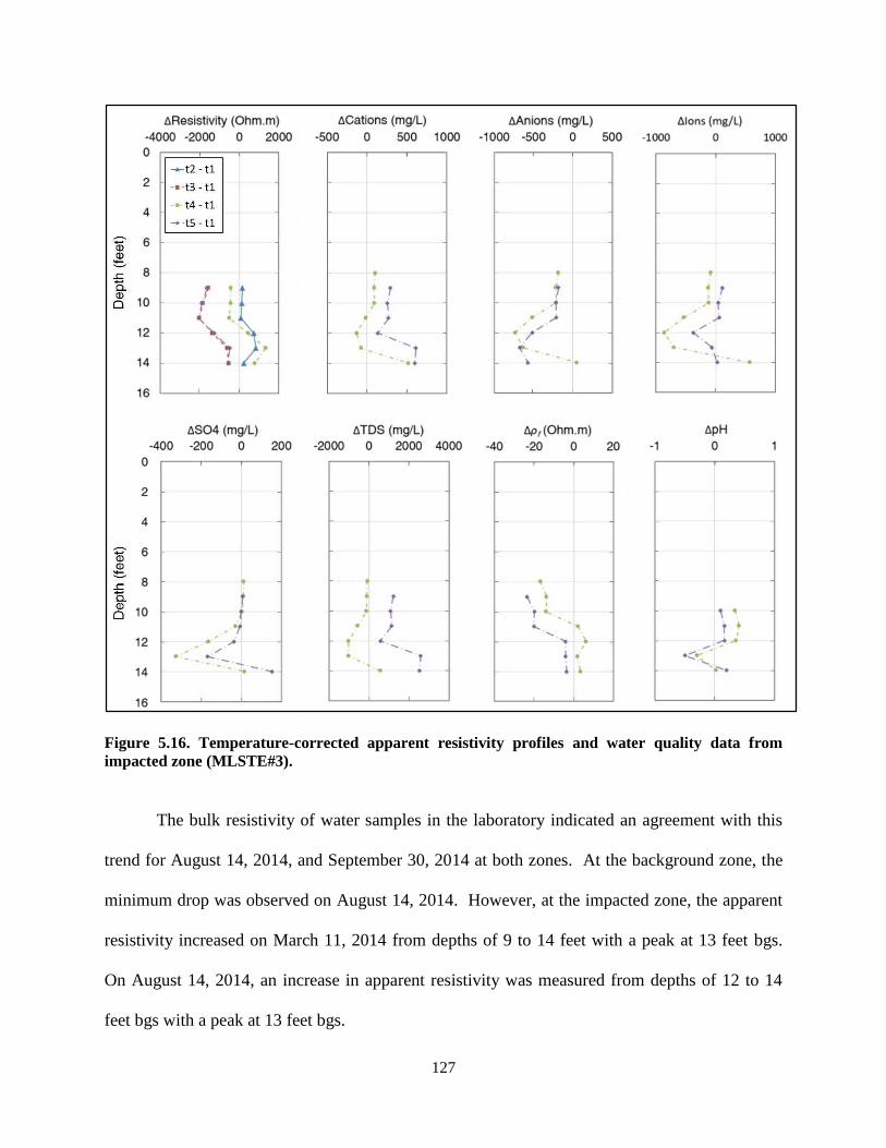
127

Figure 5.16. Temperature-corrected apparent resistivity profiles and water quality data from impacted zone (MLSTE#3).

The bulk resistivity of water samples in the laboratory indicated an agreement with this

trend for August 14, 2014, and September 30, 2014 at both zones. At the background zone, the

minimum drop was observed on August 14, 2014. However, at the impacted zone, the apparent

resistivity increased on March 11, 2014 from depths of 9 to 14 feet with a peak at 13 feet bgs.

On August 14, 2014, an increase in apparent resistivity was measured from depths of 12 to 14

feet bgs with a peak at 13 feet bgs.

128

Analysis of water samples for bulk resistivity of pore fluids, TDS, and major inorganic

ions including sulfates at background and impacted zones are shown in Figure 5.15 and Figure

5.16. At the background zone, the data indicated that the major ions were lower on August 14,

2014 than on September 30, 2104. The sulfate increased on both dates, except at 10 and 14 feet

bgs on August 14, 2014. However, the increase in sulfate concentration was less on September

30, 2014 at depths of 11, 12, and 13 feet bgs. The measured TDS increased on both dates, except

at 10 and 14 feet bgs on August 14, 2014. The measured bulk resistivity of pore fluid in the

laboratory indicated reduction in measured data on both dates, except at 14 feet bgs. The pH was

increased through the depth almost equally on both dates.

In the impacted zone, the major ion concentration decreased on both dates, except at 14

feet bgs on August 14, 2014. The reduction in major ions was more significant on August 14,

2014. The sulfate concentration indicated a slight increase on both dates, except at 12 and 13 feet

bgs. The TDS concentration reduced on August 14, 2014 because of the increase on September

30, 2014. The pH was increased on both dates, except at 13 feet bgs, a reduction was observed.

The measured apparent resistivity versus water-quality parameters acquired from the

background and impacted zones are curve fitted using the multivariate regression method. The

results are shown in Table 5.4. The results of the regression using background-zone data

indicate that Br-, NO3-, and CO3

2- provide the major influence on apparent resistivity. In the

compacted zone, K-, Br-, and CO32- have significant effect on apparent resistivity.

129

Table 5.4. Multivariate regression of ions and TDS versus apparent resistivity of formation

Parameter Coefficients

Background Zone Impacted Zone R Square 0.91416 0.969356 Adjusted R Square 0.93468 0.931051 Observations 17 19 Intercept 3389.04 3477.22 Ca 0.71 -18.59 Mg 5.05 10.29 Na -5.62 -12.65 K 35.64 95.37 Br 1032.76 330.06 CO3 -141.63 -164.77 HCO3 -3.80 0.63 Cl -8.48 50.89 SO4 0.38 -0.56 TDS 0.13 0.33

Overall, reduction of hydrocarbons in impacted zone by microbial activity changes the

geochemistry of pore fluids. Microbial activity is usually determined by various parameters

including the study of microbial community, terminal electron acceptor processes (TEAs),

production of the by-products of degradation (e.g., organic acids, carbon dioxide, and a shift in

isotopes; Atekwana 2005). However, collecting data from the above parameters is not sufficient

to correlate the electrical-resistivity signals to depletion or natural loss of LNAPL. In fact,

hydrogeological data including precipitation, discharge and recharge of groundwater, and

direction of groundwater flow are important factors contributing to the conclusion. As a result,

to create a basis for future study using electrical resistivity method to track depletion or natural

loss of hydrocarbon in a complex system, more information needs to be considered and

monitored as follows:

Proper well completion to create a uniform contact between the formation and electrodes,

Measurement of resistivity with an automated system to track continuous variation of

resistivity over time,

130

Determination of physical, chemical, and microbial conditions of the subsurface using 3G

approaches (i.e., cryogenic core collection (C3) and high-throughput analysis of frozen

core discussed in Chapters 2 and 3 of this document),

Monitoring of recharge, discharge, and precipitation at the site,

Monitoring of water content above the water table (vadose zone).


Laboratory- and field-scale investigation were performed in this study to test the

capability of vertical resistivity profiling to track depletion or natural loss of LNAPL in

unconsolidated geological formations over time. A laboratory study was performed using sand

columns. Titanium mesh electrodes were installed at the center of columns packed with

Colorado silica sand (mesh size #20 to #50). Half of the height of the sand columns were

smeared by MTBE (as an LNAPL). A vapor capture system facilitated the volatilization of

MTBE. The resistivity of sand columns was measured over a short period of time (30 days) by

imposing AC current (12 and 24 Volts, 60 Hz). Two-electrode and Wenner arrays were used for

measuring the resistivity of porous media. The results indicated a trend of NAPL depletion over

the period of measurement. Resistivity measurements of sand columns using the two-electrode

array indicated more sensitivity in comparison to the Wenner array.

A field study was performed at a former refinery in the western U.S. The site is

contaminated by a range of LNAPL over 50 years. Multilevel systems consisting of electrodes,

water sampler, and thermocouple were installed at the background zone (clean zone) and the

impacted zone. In situ measurements of complex resistivity and temperature and water sampling

were performed at both zones for almost a year. The water samples were analyzed in the

laboratory to determine geochemistry of pore fluids. The results indicated changes in resistivity

131

over time. However, to create a basis for temporal comparison of measured and analyzed data, a

few assumptions were considered. First, there are no clay minerals in the formation. Second,

electrodes are locally fixed through the depth; therefore, the formation (i.e., porosity) does not

affect the temporal measurement of apparent resistivity. Third, the formation below the water is

assumed to be 100% saturated. Last, temperature affects the bulk resistivity of pore fluids.

Based on the above assumptions, measured apparent resistivity below the water table was

corrected for temperature variation, and the effect of porosity and saturation was ignored in the

interpretation of the data. Also, the resistivity data was compared to the first set of

measurements. The results indicated decreases in apparent resistivity below the water table at

background zone. However, at impacted zone, the measured resistivity indicated both increases

and decreases through depth and time. Trends were justified by geochemistry of pore fluids

including major ions, sulfate, and TDS. For a comprehensive understanding of electrical

response of contaminated subsurface, information including microbial community, terminal

electron acceptor processes (TEAs), production of by-products of degradation (e.g., organic

acids, carbon dioxide, and a shift in isotopes can be useful. Also, hydrogeological data including

precipitation, discharge and recharge of groundwater, and direction of groundwater flow are

important factors to consider for a comprehensive conclusion.

Overall, this study reveals that application of vertical resistivity profiling at a complex

LNAPL-impacted subsurface that undergoes depletion due to natural attenuation needs to

consider many factors including proper well completion, continuous measurement of resistivity,

temperature, recharge, discharge, precipitation, water content (in the vadose zone), and bio-

physicochemical processes in the subsurface. Therefore, due to multiple factors, it appears that

132

tracking remaining LNAPL at field site is at best difficult, and potentially infeasible, using the

electrical resistivity method.

133

CHAPTER 6

SUMMARY, RECOMMENDATION, AND CONCLUSION

This chapter presents a summary of the results with respect to the hypotheses introduced

in Chapter 1 and recommendations for future work. The overarching objective of this Ph.D.

research was to advance a more comprehensive understanding of physical, chemical, and

microbial conditions in all relevant subsurface compartments using 3G methods. Seven

hypotheses were defined in Chapter 1 and all were tested through four previous chapters. The

following sections summarize the highlights of the Chapter 2 through Chapter 5. Also, a

discussion over the implication of this research is presented at the end.

Results from Chapter 2

Cryogenic Core Collection from Unconsolidated Subsurface Media

Chapter 2 tested the following hypotheses through a series of controlled experiments at a

clean site and application of the C3 method at two contaminated sites. The hypotheses are:


improve the recovery of the core by limiting losses of the sediment from the sampling tube

during withdrawal.

Hypothesis 2: In situ freezing of the unconsolidated sediments can preserve the pore

fluids within the core.

Subjectively, Hypotheses 1 and 2 were both verified. Unfortunately, absent more

complete comparison of results with and without freezing, rigorous resolution of the Hypotheses

1 and 2 is not possible and more work may be required to fully document the benefit of C3. The

following provides a summary of results and recommendations for further work.

134

A series of controlled experiments were conducted at the Drilling Engineers, Inc. facility

in Fort Collins, CO to refine the tools and method. Key elements of the C3 method include

downhole circulation of LN via a cooling system, strategic use of insulation to focus cooling into

the core, and use of back pressure to optimize cooling. Controlled experiments led to developing

two cooling systems fit inside a CME continuous sample tube system: 1) cooling coil system and

2) dual-wall cooling cylinder. The C3 operational procedure consisted of 1) advancement of the

C3 barrel 2 ½ feet, 2) injection of LN through the system to freeze the core and, ideally, the

formation of a frozen zone of sediment around the exterior of the drive shoe, 3) withdrawal of

the C3 barrel to the surface, 4) removal of the core, inspection, recovery measurement, and 5)

placing the core in a cooler with dry ice and shipping to the laboratory.

The C3 method was applied at two contaminated sites: 1) FEW in Cheyenne, WY and 2)

a former refinery in the western U.S. Through three field efforts and five days of drilling, 146

feet of frozen core were collected. The average cryogenic core production rate was about 30

foot/day. Based on prior HSA coring at both sites, C3 required approximately one and half as

much time as traditional HSA drilling. This extra time needs to be balanced against the

improved recovery from targeted intervals using the C3 method and the preservation of key

attributes, including fluid saturations (see Section 2.5.3).

At FEW, recovery of the core was almost 100%, except for intervals encountering caliche

beds that required a center head in lieu of the continuous sample tube system. At the former

refinery, recovery varied from 16% to 100% with a median of 80%. The primary factor limiting

recovery at the former refinery was cobbles that were larger than the 2 ½-inch ID drive shoe that

blocked sediment entry into the sample systems. Attempts to collect sediment core at the former

refinery, using the 2 ½-inch ID CME continuous sample tube system without the cryogenic

135

cooling system consistently yielded extremely poor recovery (less than 15%). The time of

injecting LN through the system to freeze the core averaged five minutes for freezing a 2 ½-foot

core above and below the water table.

At the former refinery, control of flowing sand was evaluated on several runs by

measuring the solids level in the HSA after the removal of the C3 barrel. Preliminary results

indicated that the dual-wall cooling system reduced the amount of sediment entering the barrel

between core collection runs.

High-throughput analysis (HTA) of the frozen core collected at the former refinery was

performed in the laboratory to determine fluid saturation (i.e., aqueous, non-aqueous liquid, and

gas) and porosity above and below the water table. The combined processes of C3 and HTA

allow all core processing to be conducted in the laboratory, versus in the field, and on a

timeframe that is flexible (i.e., because the core is kept frozen). Other advantages of laboratory

processing include 1) elimination of weather-related sample biases, 2) access to better

environmental controls (e.g., hoods, gloves, etc.), 3) improved accuracy of measurements (e.g.,

weights and volumes), and 4) enhanced safety associated with not deploying staff to field sites.

Critically, given in situ freezing, the results are not biased by drainage of pore fluids from the

core during sample collection. Measured porosity indicated median values of 23.7% and 29.2%

above and below the water table, respectively. Water saturation resulted in median values of

49.5% to 74.5% above and below the water table, respectively. For gas saturation, median values

of 50.5% and 22.9% were estimated above and below the water table, respectively. LNAPL

saturations were measured with median values of 0.6% and 2.8% for above and below the water

table, respectively. Lower porosity values reflect samples where large pieces of solid aggregate

136

comprised a large fraction of the sample. Large gas saturations below the water table are

attributed to gases being generated by anaerobic natural source zone depletion processes.

Overall, the results of Chapter 2 indicated that C3 and HTA of frozen core can facilitate

better resolution of subsurface contaminants, leading to enhanced site conceptual models.

However, further work needs to improve the field application of the C3 method and the

laboratory-based HTA of frozen core. Therefore, followings are recommended for future work:

Refinement of the C3 cooling barrel to provide a larger space for LN,

Increase in the size of LN delivery line,

Better insulation of the system to focus the energy into the sediment core,

New versions of C3 barrel to control flowing sand in unconsolidated geological

formations below the water table,

Provision of two sets of tools to minimize the time of operation in the field.


Cryogenic Core Collection and High-Throughput Analysis of Frozen Core

The 3G site characterization approach, including the C3 method and HTA of frozen core

in the laboratory, was applied at FEW (in Cheyenne, WY), a DNAPL-contaminated site. This

study was performed to test the following hypothesis:




Hypothesis 3 was verified with the qualification that studies were conducted using adjacent

boring versus the infeasible alternative of conducting comparative studies using the same

137

sample. The following provides a summary of related results and recommendations for further

work.

3G methods were applied (in 2014) at three locations (MW38, MW173, and MW700) at

FEW where the 2G methods were applied in 2010. 2G methods included Membrane Interface

Probe (MIP), Waterloo ProfilerTM, continuous sediment coring and analysis of sub-samples

collected from the core, and installation of a multilevel sampling system for monitoring the

plume.

Following Sale et al. (2013), the results of 2G methods applied in 2010 indicated that

laboratory analysis of the preserved sub-sample provided from low-k intervals was the only

promising method that could estimate fluid saturation. However, this method was biased by the

drainage of pore fluids due to the limitation of conventional coring, in particular, in transmissive

zones. Also, flowing sand into the drilled space can compromise the recovery of the targeted

interval and the estimate of key attributes.

Application of the C3 method for two days led to the collection of 50 feet of frozen core

with the rate of 25 foot/day. The average of five minutes of injecting LN was enough to freeze a

2 ½-foot core above and below the water table. Except for intervals encountering caliche layers

that required a center head in lieu of the continuous sample tube system, recovery was close to

100%.

HTA of the frozen core including core processing and sub-sampling, preserving sub-

samples, and analysis of subsamples was conducted in the laboratory to determine physical,

chemical, and microbial properties of the samples. The typical time requirement to process a 2

½-foot frozen core was about 30 minutes. This time was sufficient for the completion of

processing while allowing only minor surficial thawing of the frozen core.

138

Analysis of the sub-samples indicated that TCE was detected at MW38, but

concentrations were lower than 50 μg/kg. There were no clear correlations between TCE and

sediment type. Methane was not detected at this location, and ORP values were higher than other

locations (i.e., MW700 and MW173). At MW173, TCE was detected at concentrations as high

as 100 μg/kg. Methane was observed in transmissive zones, potentially associated with lactate

injection near the well in the late 2000s. TCE concentrations were generally lower in

transmissive versus low-k zones, perhaps reflecting preferential delivery of lactate to the

transmissive zones. At MW173, ORP values were lower than at MW38 and followed observed

methane values. At MW700, TCE concentrations were highest (~400 μg/kg) in the transmissive

zone. The highest detected methane concentrations were also at this location (~21,000 mg/kg) in

the low-k zone. Below the water table, an inverse correlation between methane and TCE

suggests active treatment in low-k zones.

Collectively, C3 of unconsolidated geological formation and HTA of frozen core in the

laboratory provided high-density data of all contaminant compartment as well as data of the

microbial ecology. Acquiring a large amount of data from the actual subsurface condition leads

to improved site conceptual models and facilitates decision making with regard to management

of contaminated sites. However, more investigation is recommended as follows:

Refinement of the C3 tools and method as recommended in the previous section,

Improvement of the core processing methods to avoid cross contamination,

Improvement of the weight and volume measurement of sub-samples,

Analysis of frozen core using non-destructive scanning methods (e.g., NMR and CT

scan) to resolve pore geometry, as well as fluid saturation of the core.

More comparisons of analyses of core collected with and without freezing.

139


Spatial Distribution Analysis of Non-Aqueous Phase Liquid in Porous Media Using

Nuclear Magnetic Resonance: Laboratory and Field Studies

Laboratory- and field-scale study of NMR was performed in Chapter 4 to test the following

hypotheses:

Hypothesis 4: Freezing the water, while keeping the NAPL in a liquid state, selectively

suppresses the NMR signal of water-bound hydrogen within the porous media.

Hypothesis 5: The selective freezing of water enables resolution of NAPL distribution

within the frozen sediment core, both qualitatively and quantitatively.


qualitatively discriminate LNAPL from water in situ, using short- and long-echo times.

Hypothesis 4 was verified. Hypothesis 5 was validated with respect to qualitative delineation of

NAPL but failed with respect to quantitative resolution of NAPL. Hypothesis 6 was shown to be

incorrect. The following elucidates results and provide recommendations for further work.

The laboratory study was performed on 2-inch diameter and 2-inch long fabricated

sediment core consisting of Colorado silica sand (mesh size #20-#50) saturated with DI-water

and TCE. The core was scanned and imaged by a BRUKER small-animal scanner (2.3 Tesla,

100 MHz) at room temperature (20 °C), while the core was frozen at -25 °C. The acquired

images indicated that freezing the water within the core suppressed the NMR signals of water-

bound hydrogen. However, the hydrogen associated with TCE was still detectable since the TCE

was in liquid state (melting point of TCE is -73 °C). Therefore, freezing the porous media is an

alternative to discriminate water from NAPL (such as TCE) using the NMR method.

140

Quantification of TCE mass distribution within the frozen core using the NMR method

was evaluated on the TCE-contaminated sediment core fabricated in the laboratory. A one-

dimensional NMR scanning method (Watson 2013) was used for this study. The intrinsic signal

intensities of NMR measurements were determined using a FORTRAN code that employs the

non-parametric regression method. A comparison between the non-parametric regression and

the parametric regression on a NMR study of a core saturated with TCE indicated advantages of

the non-parametric method. A GUI MATLAB was developed for quantification of TCE within

the sediment core using NMR measurement data. However, poor accuracy in the quantification

of TCE mass within the sediment core was observed. Therefore, series of experiments were

performed on pure TCE, sand saturated with TCE, and glass beads saturated with TCE to figure

out the source of inconsistency. Further research is needed to increase the accuracy of NAPL

quantification within porous media.

Downhole NMR logging of the LNAPL-contaminated site was performed at a former

refinery in the western U.S. Monitoring wells with PVC casing were logged at the background

(clean) zone, as well as LNAPL impacted zone, using Javelin NMR tools (Vista Clara, Inc.).

NMR logging of the background zone indicated detection of water-bound hydrogen signals.

NMR logging of the impacted zone at SS-26d indicated sufficient resolution below the water

table (8 m bgs). However, the level of noise at the impacted zone (20-30%) prevented signal

detection.

Discrimination of water and LNAPL using downhole NMR logging tools was tested at

two monitoring wells (SS-45 and SS-15). Application of short- and long-echo times was not

successful due to insufficiently detected signals. Potential factors leading to this failure could be

the high level of noise stemming from the active facilities at the site and power lines passing

141

over the site, fine grain sediments that compromise the NMR signals, and the inability of NMR

logging tools to excite the hydrogen and detect the signals.

Overall, suppressing NMR signals of water-bound hydrogen by freezing the water brings

a novel approach for discrimination of NAPL from water using the NMR method. However,

further work is needed for the quantification of NAPL within the porous media both in the

laboratory and field. Therefore, the following suggestions are recommended for future work:

Using a rock/sediment core scanner (e.g., Magritek NMR core analyzer and GeoSpec2

core analyzer) that is designed to study pore geometry as well as pore fluids of porous

media. These scanners are able to control the temperature of the core during the scanning

time.

NMR study of targeted nuclei associated with the contaminant (e.g., Cl in chlorinated

solvents) is proposed using a suitable Chlorine-NMR scanner.


Monitoring Depletion of Light Non-Aqueous Phase Liquid in Shallow Geological

Formation Using Electrical Resistivity

Vertical resistivity profiling was studied in both laboratory- and field-scale experiments.

The following hypothesis was tested through this study:



Hypothesis 7 was shown to be incorrect. The following provides a summary of related results

and recommendations for further work.

A laboratory experiment was performed to evaluate the electrical response of

unconsolidated porous media while LNAPL is being depleted over a short period of time (about

142

30 days). Sand columns (Colorado silica sand, mesh size #10 to #20, φ=0.3) contaminated with

methyl tert-butyl ether (MTBE, an LNAPL) were studied. A multilevel electrode system was

used to measure the electrical resistivity of impacted porous media by imposing AC current (12

V and 24 V, 60 Hz). Two- and four-electrode (Wenner) arrays were used for measuring

resistivity of porous media. The trend of reduction in resistivity over time indicated depletion of

LNAPL. This reduction in measured apparent resistivity was in agreement with the insulation

layer model according to the literature while the LNAPL did not change physicochemically. In

contrast to the literature, the results indicated that resistivity measurement using the two-

electrode array was more sensitive in comparison with the Wenner array in the column

experiment. One may attribute this discrepancy to the boundary condition and energy storage

within the confined porous media that needs more investigation.

The field experiment was performed at the former refinery in the western U.S. The site is

contaminated by LNAPL over a period of 50 years. Multilevel systems consisting electrodes,

water sampler, and thermocouple were installed at the background zone (clean zone) and the

impacted zone. In situ measurements of resistivity and temperature and water sampling were

performed within almost a year. Complex resistivity was measured in this study using an LCR

meter. The water samples were analyzed in laboratories at CSU to determine the geochemistry

of pore fluids. The results indicated change in resistivity over time. However, to create a basis

for temporal comparison of measured and analyzed data, a few assumptions were considered: 1)

there are no clay minerals in the formation, 2) electrodes are locally fixed through the depth;

therefore, the formation (i.e., porosity) does not affect the temporal measurement of apparent

resistivity, 3) the formation below the water is assumed to be 100% saturated, and 4) temperature

affects the bulk resistivity of pore fluids.

143

The results indicated a decrease in apparent resistivity below the water table at

background zone as well as the impacted zone over time. This trend is justified by the

geochemistry of pore fluids. However, change in the geochemistry of the zones can occur due to

change in physical and biogeochemical conditions. For instance, recharge condition, and

consequentially water fluctuations, can change the geochemistry of pore fluids.

Overall, this study revealed that the application of the vertical resistivity profiling at such

a complex system that is undergoing depletion or natural attenuation of LNAPL needs to

consider many parameters. Degradation of hydrocarbons in the impacted zone by microbial

activity changes the geochemistry of pore fluids. Microbial activity is usually determined by

various parameters including study of microbial community, terminal electron acceptor

processes (TEAs), production of by-products of degradation. However, collecting data from the

above parameters is not sufficient to correlate the electrical resistivity signals to natural losses.

In fact, hydrogeological data including precipitation, discharge and recharge of groundwater, and

direction of groundwater flow are important factors contributing to the conclusion. As a result,

future study using electrical resistivity methods to track depletion or natural loss of hydrocarbon

in an aged LNAPL-contaminated site needs to consider and monitor more factors including:

Proper well completion to create a uniform contact between the formation and electrodes,

Measurement of resistivity with an automated system to track continuous variation of

resistivity over time,

Determination of physical, chemical, and microbial condition of the subsurface using the

3G approach (i.e., cryogenic core collection (C3) and high-throughput analysis of frozen

core discussed in Chapters 2 and 3 of this document),

Monitoring of recharge, discharge, and precipitation at the site,

144

Monitoring of water content above the water table (vadose zone).

Implications

At the time of writing this dissertation, the primary risks posed by many subsurface

releases have been addressed and greater reliance is being placed on natural depletion of

contaminants. Methods described herein provide an improved basis for demonstrating, and

responsibly relying on, natural depletion of contaminants as a remedy for the risk that remains

after decades of active and natural depletion of subsurface releases.

145

REFERENCES

Abdel Aal, G.Z. and Atekwana, E.A. (2014). ″Spectral induced polarization (SIP) response of

biodegraded oil in porous media.″ Geophysical Journal International, 196(2), 804-817,

doi:10.1093/gji/ggt416.

Abdel Aal, G.Z., Atekwana, E.A., Slater, L.D., and Atekwana, E.A. (2004). ″Effects of microbial

processes on electrolytic and interfacial electrical properties of unconsolidated

sediments.″ Geophysical Research Letters, 31(12), doi:10.1029/2004GL020030.

Abdel Aal, G.Z., Slater, L.D., and Atekwana, E.A. (2006). ″Induced-polarization measurements

on unconsolidated sediments from a site of active hydrocarbon biodegradation.″

Geophysics, 71(2), H13-H24. doi:10.1190/1.2187760.

Akhbari, D. (2013). ″Thermal aspects of STELA (sustainable thermally enhanced LNAPL

attenuation).″ M.Sc. thesis, Department of Civil and Environmental Engineering,

Colorado State University (CSU), Fort Collins, CO, USA.

Akkurt, R., Mardon, D., Gardner, J.S., Marschall, D.M., and Solanet, F. (1998). ″Enhanced

diffusion: expanding the range of NMR direct hydrocarbon-typing application.″ SPWLA

39th Annual Logging Symposium, Keystone, CO, USA.

Allen, J.P., Atekwana, E.A., Atekwana, E.A., Duris, J.W., Werkema, D.D., and Rossbach, S.

(2007). ″The microbial community structure in petroleum-contaminated sediments

corresponds to geophysical signatures.″ Applied and Environmental Microbiology, 73(9),

2860-2870, doi:10.1128/aem.01752-06.

146

Amos, R.T. and Mayer, K.U. (2006). ″Investigating ebullition in a sand column using dissolved

gas analysis and reactive transport modeling.″ Environmental Science & Technology,

40(17), 5361-5367, doi:10.1021/es0602501.

Araujo, M., Hunger, M., and Martin, R. (1989). ″Nuclear magnetic relaxation of protons in

Venezuelan crude oil.″ Fuel, 68(8), 1079-1081, doi:10.1016/0016-2361(89)90080-x.

Archie, G.E. (1942). ″The electrical resistivity log as an aid in determining some reservoir

characteristics.″ Transactions of the American Institute of Mining and Metallurgical

Engineers, 146, 54-61, doi:10.1007/s10712-009-9089-8.

Atekwana, E.A. and Atekwana, E.A. (2010). ″Geophysical signatures of microbial activity at

hydrocarbon contaminated sites: a review.″ Surveys in Geophysics, 31(2), 247-283.

Atekwana, E.A., Atekwana, E.A., Legall, F.D., and Krishnamurthy, R.V. (2004d). ″Field

evidence for geophysical detection of subsurface zones of enhanced microbial activity.″

Geophysical Research Letters, 31(23), doi:10.1029/2004gl021576.

Atekwana, E.A., Atekwana, E.A., Legall, F.D., and Krishnamurthy, R.V. (2005).

″Biodegradation and mineral weathering controls on bulk electrical conductivity in a

shallow hydrocarbon contaminated aquifer.″ Journal of Contaminant Hydrology, 80(3-4),

149-167, doi:10.1016/j.jconhyd.2005.06.009.

Atekwana, E.A., Atekwana, E.A., Rowe, R.S., Werkema, D.D., and Legall, F.D. (2004b). ″The

relationship of total dissolved solids measurements to bulk electrical conductivity in an

aquifer contaminated with hydrocarbon.″ Journal of Applied Geophysics, 56(4), 281-294,

doi:10.1016/j.jappgeo.2004.08.003.

Atekwana, E.A., Atekwana, E.A., Werkema, D.D., Duris, J., Rossbach, S., Sauck, W.A.,

Koretsky, C., Cassidy, D., Means, J., and Sherrod, L. (2003). ″Investigating the effects of

147

microbial communities on electrical properties of soils: preliminary results from a pilot

scale column experiment.″ In EGS-AGU-EUG Joint Assembly, Nice, France.

Atekwana, E.A., Sauck, W.A., and Werkema, D.D. (1998). ″Characterization of a complex

refinery groundwater contamination plume using multiple geoelectric methods.″ In

Proceedings of the Symposium on the Application of Geophysics to Environmental and

Engineering Problems, 427-436.

Atekwana, E.A., Sauck, W.A., and Werkema, D.D. (2000). ″Investigations of geoelectrical

signatures at a hydrocarbon contaminated site.″ Journal of Applied Geophysics, 44(2-3),

167-180, doi:10.1016/s0926-9851(98)00033-0.

Atekwana, E.A., Werkema, D.D., Allen, J.P., Smart, L.A., Duris, J.W., Cassidy, D.P., Sauck,

W.A., and Rossbach, S. (2004c). ″Evidence for microbial enhanced electrical

conductivity in hydrocarbon-contaminated sediments.″ Geophysical Research Letters,

31(23), doi:10.1029/2004gl021359.

Atekwana, E.A., Werkema, D.D., and Atekwana, E.A. (2006). ″Biogeophysics: the effects of

microbial processes on geophysical properties of the shallow subsurface.″ Applied

Hydrogeophysics, Springer, 161-193.

Atekwana, E.A., Werkema, D.D., Duris, J.W., Rossbach, S., Sauck, W.A., Cassidy, D.P., Means,

J., and Legall, F.D. (2004a). ″In situ apparent conductivity measurements and microbial

population distribution at a hydrocarbon-contaminated site.″ Geophysics, 69(1), 56-63,

doi:10.1190/1.1649375.

Balcom, B.J., Fischer, A.E., Carpenter, T.A., and Hall, L.D. (1993). ″Diffusion in aqueous gels,

mutual diffusion coeff icients measured by one-dimensional nuclear magnetic resonance

148

imaging.″ Journal of the American Chemical Society, 115(8), 3300-3305,

doi:10.1021/ja00061a031.

Benson, A.K. and Mutsoe, N.B. (1996). ″DC resistivity, ground penetrating radar, and soil and

water quality data combined to assess hydrocarbon contamination: a case study.″

Environmental Geosciences, 3(4), 165-175.

Bermejo, J.L., Sauck, W.A., and Atekwana, E.A. (1997). ″Geophysical discovery of a new

LNAPL plume at the former Wurtsmith AFB, Oscoda, Michigan.″ Ground Water

Monitoring and Remediation, 17(4), 131-137.

Callaghan, P.T. (1991). ″Principles of nuclear magnetic resonance microscopy.″ Oxford

University Press, New York, USA

Callaghan, P.T. (2011). ″Translational dynamics and magnetic resonance: principles of pulsed

gradient spin echo NMR.″ Oxford University Press, New York, USA.

Cassidy, D.P., Werkema, D.D., Sauck, W.A., Atekwana, E.A., Rossbach, S., and Duris, J.

(2001). ″The effects of LNAPL biodegradation products on electrical conductivity

measurements.″ Journal of Environmental and Engineering Geophysics, 6(1), 47-52.

Chen, J.D., Dias, M.M., Patz, S., and Schwartz, L.M. (1988). ″Magnetic resonance imaging of

immiscible-fluid displacement in porous media.″ Physical Review Letters, 61(13), 1489-

1492, doi:10.1103/PhysRevLett.61.1489.

Chen, Q., Kinzelbach, W., and Oswald, S. (2002). ″Nuclear magnetic resonance imaging for

studies of flow and transport in porous media.″ Journal of Environmental Quality, 31(2),

477-486.

Chu, Y.J., Werth, C.J., Valocchi, A.J., Yoon, H., and Webb, A.G. (2004). ″Magnetic resonance

imaging of nonaqueous phase liquid during soil vapor extraction in heterogeneous porous

149

media.″ Journal of Contaminant Hydrology, 73(1-4), 15-37,

doi:10.1016/j.jconhyd.2003.12.003.

Coates, G.R., Xiao, L., and Prammer, M.G. (1999). ″NMR logging principles and applications.″

Halliburton Energy Services, Houston, USA.

Cohen, R.M., Bryda, A.P., Shaw, S.T., and Spalding, C.P. (1992). ″Ecaluation of visual methods

to detect NAPL in soil and water.″ Ground Water Monitoring and Remediation, 12(4),

132-141, doi:10.1111/j.1745-6592.1992.tb00072.x.

Daniels, J.J., Roberts, R., and Vendl, M. (1992). ″Site studies of ground penetrating radar for

monitoring petroleum product contaminants.″ In Proceedings of the Symposium on the

Application of Geophysics to Engineering and Environmental Problems, 2, 597.

Davies, S., Hardwick, A., Roberts, D., Spowage, K., and Packer, K.J. (1994). ″Quantification of

oil and water in preserved reservoir rock by NMR spectroscopy and imaging.″ Magnetic

Resonance Imaging, 12(2), 349-353, doi:10.1016/0730-725x(94)91554-7.

Davis, C.A., Atekwana, E.A., Slater, L.D., Rossbach, S., and Mormile, M.R. (2006). ″Microbial

growth and biofilm formation in geologic media is detected with complex conductivity

measurements.″ Geophysical Research Letters, 33(18), doi:10.1029/2006gl027312.

de Castro, D.L., and Branco, R.M.G.C. (2003). ″4-D ground penetrating radar monitoring of a

hydrocarbon leakage site in Fortaleza (Brazil) during its remediation process: a case

history.″ Journal of Applied Geophysics, 54(1-2), 127-144,

doi:10.1016/j.jappgeo.2003.08.021.

de Ryck, S.M., Redman, J.D., and Annan, A.P. (1993). ″Geophysical monitoring of a controlled

kerosene spill.″ In Proceedings of the sixth Symposium on the Application of Geophysics

to Engineering and Environmental Problems, 5-119, San Diego, USA.

150

Dunn, K.J., Bergman, D.J., and LaTorraca, G.A. (Eds.). (2002). ″Nuclear magnetic resonance:

petrophysical and logging applications.″ Elsevier, UK.

Durnford, D., Brookman, J., Billica, J., and Milligan, J. (1991). ″LNAPL distribution in a

cohesionless soil: a field investigation and cryogenic sampler.″ Ground Water

Monitoring and Remediation, 11(3), 115-122, doi:10.1111/j.1745-6592.1991.tb00387.x.

Ellis, D.V. and Singer, J.M. (2007). ″Well logging for earth scientists.″ Springer, Dordrecht,

Netherlands.

Endres, A.L. and Greenhouse, J.P. (1996). ″Detection and monitoring of chlorinated solvent

contamination by thermal neutron logging.″ Ground Water, 34(2), 283-292,

doi:10.1111/j.1745-6584.1996.tb01888.x.

Endres, A.L. and Redman, J.D. (1993). ″Modelling the electrical properties of porous rocks and

soils containing immiscible contaminants.″ In Proceedings of the sixth Symposium on the

Application of Geophysics to Engineering and Environmental Problems, 1(B), 105-112,

San Diego, USA.

Farrar, T.C. and Becker, E.D. (1971). ″Pulse and Fourier transform NMR: introduction to theory

and methods.″ Academic Press, Florida, USA.

Fischer, A., Muller, M., and Klasmeier, J. (2004). ″Determination of Henry's law constant for

methyl tert-butyl ether (MTBE) at groundwater temperatures.″ Chemosphere, 54(6), 689-

694, doi:10.1016/j.chemosphere.2003.08.025.

Geoprobe. (2011). ″DT325 Dual Tube Sampling System SOP System.″ Retrieved from

http://geoprobe.com/literature/dt325-dual-tube-samplingsystem-sop.

151

Guilbeault, M.A., Parker, B.L., and Cherry, J.A. (2005). ″Mass and flux distributions from

DNAPL zones in sandy aquifers.″ Ground Water, 43(1), 70-86, doi:10.1111/j.1745-

6584.2005.tb02287.x.

Irianni Renno, M., Akhbari, D., Olson, M.R., Byrne, A.P., Lefèvre, E., Zimbron, J., Lyverse, M.,

Sale, T.C., De Long, S.K. (2015). ″Comparison of bacterial and archaeal communities in

depth-resolved zones in an LNAPL body.″ Applied Microbiology and Biotechnology, 1-

14, doi: 10.1007/s00253-015-7106-z.

James, T.L. (1998). ″Fundamentals of NMR.″ Department of Pharmaceutical Chemistry,

University of California, San Francisco, USA.

Johnson, R.L., Brow, C.N., Johnson, R.O., and Simon, H.M. (2013). ″Cryogenic core collection

and preservation of subsurface samples for biomolecular analysis.″ Ground Water

Monitoring and Remediation, 33(2), 38-43, doi:10.1111/j.1745-6592.2012.01424.x.

Kearey, P., Brooks, M., and Hill, I. (2009). ″An introduction to geophysical exploration.″ Wiley-

Blackwell, Hoboken, USA.

Keating, K. (2014). ″A laboratory study to determine the effect of surface area and bead diameter

on NMR relaxation rates of glass bead packs.″ Near Surface Geophysics, 12(2), 243-254,

doi:10.3997/1873-0604.2013064.

Kiaalhosseini, S., Johnson, R.L., Rogers, R.C., Irianni renno, M., Lyverse, M., and Sale, T.C.

(submitted in 2016). ″Cryogenic core collection (C3) from unconsolidated subsurface

media.″ Accepted by Journal of Groundwater Monitoring & Remediation, May 2016.

Kiaalhosseini, S., Sale T.C., Johnson, R.L., Olson, M.R., and Rogers, R.C. (2015). ″Cryogenic

core collection (C3).″ University Consortium for Field-Focused Groundwater

152

Contamination Research Program for Annual Progress Meeting, University of Guelph,

Guelph, Canada, (Oral).

Kleinberg, R.L. and Jackson, J.A. (2001). ″An introduction to the history of NMR well logging.″

Concepts in Magnetic Resonance, 13(6), 340-342.

Levitt, M. H. (2008). ″Spin dynamics: basics of nuclear magnetic resonance.″ 2nd edition, John

Wiley & Sons, New York, USA.

Li, L., Marica, F., Chen, Q., MacMillan, B., and Balcom, B.J. (2007). ″Quantitative

discrimination of water and hydrocarbons in porous media by magnetization prepared

centric-scan SPRITE.″ Journal of Magnetic Resonance, 186(2), 282-292,

doi:10.1016/j.jmr.2007.03.008.

McNeill, J.D. (1980). ″Electrical conductivity of soils and rocks.″ Geonics Limited, Ontario,

Canada.

Mewafy, F.M., Werkema, D.D., Atekwana, E.A., Slater, L.D., Abdel Aal, G.Z., Revil, A., and

Ntarlagiannis, D. (2013). ″Evidence that bio-metallic mineral precipitation enhances the

complex conductivity response at a hydrocarbon contaminated site.″ Journal of Applied

Geophysics, 98, 113-123, doi:10.1016/j.jappgeo.2013.08.011.

Milsom, J. and Eriksen, A. (2011). ″Field geophysics.″ 4th edition, John Wiley & Sons, New

Jersey, USA.

Monier-Williams, M. (1995). ″Properties of light non-aqueous phase liquids and detection using

commonly applied shallow sensing geophysical techniques.″ In Proceedings of the

Symposium on the Application of Geophysics to Engineering and Environmental

Problems, 1-13, Orlando, FL, USA.

153

Murphy, F. and Herkelrath, W.N. (1996). ″A sample-freezing drive shoe for a wire line piston

core sampler.″ Ground Water Monitoring and Remediation, 16(3), 86-90,

doi:10.1111/j.1745-6592.1996.tb00143.x.

NRC (2005). ″Contaminants in the subsurface; source zone assessment and remediation.″ The

National Academies Press, Washington DC, USA.

NRC (2013). ″Alternatives for managing the nation's complex contaminated groundwater sites.″

The National Academies Press, Washington DC, USA.

Olhoeft, G.R. (1992). ″Geophysical Detection Of Hydrocarbon And Organic Chemical

Contamination.″ In Proceedings of the Fifth Symposium on the Application of Geophysics

to Engineering and Environmental Problems, 587-595, Oakbrook, IL, USA.

Pervizpour, M., Pamukcu, S., and Moo-Young, H. (1999). ″Magnetic resonance imaging of

hydrocarbon-contaminated porous media.″ Journal of Computing in Civil Engineering,

13(2), 96-102, doi:10.1061/(asce)0887-3801(1999)13:2(96).

Ranhong, X. and Lizhi, X. (2011). ″Advanced fluid-typing methods for NMR logging.″

Petroleum Science, 8(2), 163-169, doi:10.1007/s12182-011-0130-4.

Reynolds, J.M. (2011). ″An introduction to applied and environmental geophysics.″ Wiley-

Blackwell, Chichester, UK.

Rothwell, W.P. and Vinegar, H.J. (1985). ″Petrophysical application of NMR imaging.″ Applied

Optics, 24(23), 3969-3972.

Sale et al. (2006). ″Electronically Induced Redox Barriers for Treatment of Groundwater.″ Cost

and Performance Report, U.S. Department of Defense (DOD), Environmental Security

Technology Certificate Program (ESTCP), ER-0112.

154

Sale, T.C. and Johnson, R.L. (2012). ″Third-generation (3G) site characterization; cryogenic core

collection and high-throughput core analysis.″ White paper, Extended Scope for Basic

Research Addressing Contaminants in Low Permeability Zones, U.S. Department of

Defense (DOD), Strategic Environmental Research and Development Program (SERDP),

ER-1740.

Sale, T.C., Kiaalhosseini, S., Olson, M., & Johnson, R.L. (2015). ″Management of contaminants

stored in low permeability zones: a state-of-the-science review, part II, third-generation

(3G) site characterization: cryogenic core collection and high-throughput core analysis.″

U.S. Department of Defense (DOD), Strategic Environmental Research and Development

Program (SERDP), ER-1740.

Sale, T.C. and Newell, C.J. (2011). ″Guide for selecting remedies for subsurface releases of

chlorinated solvents.″ Project Report Prepared for the Environmental Security Testing

Certification and Program (ESTCP).

Sale, T.C., Parker, B.L., Newell, C.J., Devlin, J.F., Adamson, D., Chapman, S., and Saller, K.

(2013). ″ Management of contaminants stored in low permeability zones: a state-of-the-

science review.″ U.S. Department of Defense (DOD), Strategic Environmental Research

and Development Program (SERDP), ER-1740.

Sauck, W.A. (2000). ″A model for the resistivity structure of LNAPL plumes and their environs

in sandy sediments.″ Journal of Applied Geophysics, 44(2-3), 151-165,

doi:10.1016/s0926-9851(99)00021-x.

Sauck, W.A., Atekwana, E.A., and Nash, M.S. (1998). ″High conductivities associated with an

LNAPL plume imaged by integrated geophysical techniques.″ Journal of Environmental

and Engineering Geophysics, 2(3), 203-212.

155

Schneider, G.W. and Greenhouse, J.P. (1992). ″Geophysical detection of perchloroethylene in a

sandy aquifer using resistivity and nuclear logging techniques.″ In Proceedings of the

Symposium on the Application of Geophysics to Engineering and Environmental

Problems, Oakbrook, IL, USA.

Sterrett, R.J. (2007). ″Groundwater and wells.″ Johnson Screens.

Stroo, H.F., Vogel, C.M., and Ward, C.H. (2014). ″Chlorinated solvent source zone

remediation.″ Kueper, B.H. (Ed.). Springer.

Stroo, H.F. and Ward, C.H. (2010). ″In situ remediation of chlorinated solvent plumes.″ Springer

Science & Business Media, New York, USA.

Szalai, S. and Szarka, L. (2008). ″On the classification of surface geoelectric arrays.″

Geophysical Prospecting, 56(2), 159-175, doi:10.1111/j.1365-2478.2007.00673.x.

Telford, W. M., Geldart, L. P., and Sheriff, R. E. (1990). ″Applied geophysics.″ 2nd edition,

Cambridge University Press, Cambridge, UK.

Uh, J. and Watson, A.T. (2014). ″A non-parametric approach for determining NMR relaxation

distributions.″ Transport in Porous Media, 105(1), 141-170, doi: 10.1007/s11242-014-

0364-x.

Walsh, D., Turner, P., Grunewald, E., Zhang, H., Butler Jr., J. J., Reboulet, E., Knobbe, S.,

Christy, T., Lane Jr., J.W., Johnson, C.D., Munday, T., Fitzpatrick, A. (2013). ″A small-

diameter NMR logging tool for groundwater investigations.″ Groundwater, 51(6), 914-

926, doi:10.1111/gwat.12024.

Watson, A.T. (2013). ″Development of one-dimensional imaging.″ Department of Chemical and

Biological Engineering, Colorado State University, Fort Collins, CO, USA.

156

Watson, A.T. and Chang, C.T.P. (1997). ″Characterizing porous media with NMR methods.″

Progress in Nuclear Magnetic Resonance Spectroscopy, 31(4), 343-386,

doi:10.1016/s0079-6565(97)00053-8.

Watson, A.T. and Mudra, J. (1994). ″Characterization of Devonian shales with X-ray-computed

tomography.″ SPE Formation Evaluation, 9(03), 209-212.

Wenner, F. (1915). ″A method of measuring earth resistivity.″ U.S. Bureau of Standards

Bulletin, 12, 469-478.

Werkema, D.D., Atekwana, E.A., Endres, A.L., and Sauck, W.A. (2002). ″Temporal and spatial

variability of high resolution in situ vertical apparent resistivity measurements at a

LNAPL impacted site.″ In Proceedings of Symposium on the Application of Geophysics

to Engineering and Environmental Problems.

Werkema, D.D., Atekwana, E.A., Endres, A.L., Sauck, W.A., and Cassidy, D.P. (2003).

″Investigating the geoelectrical response of hydrocarbon contamination undergoing

biodegradation.″ Geophysical Research Letters, 30(12), doi:10.1029/2003gl017346.

Whitby, C. and Skovhus, T.L. (2011). ″Applied microbiology and molecular biology in oilfield

systems.″ Springer.

Yang, C.H., Yu, C.Y., and Su, S.W. (2007). ″High resistivities associated with a newly formed

LNAPL plume imaged by geoelectric techniques: a case study.″ Journal of the Chinese

Institute of Engineers, 30(1), 53-62, doi:10.1080/02533839.2007.9671230.

Yoshimi, Y., Tokimatsu, K., Kaneko, O., and Makihara, Y. (1984). ″Undrained cyclic shear

strength of a dense Niigata sand.″ Soils and Foundations, 24(4), 131-145.

157

Zapico, M.M., Vales, S., and Cherry, J.A. (1987). ″A wireline piston core barrel for sampling

cohesionless sand and gravel below the water table.″ Ground Water Monitoring and

Remediation, 7(3), 74-82, doi:10.1111/j.1745-6592.19.

Zeman, N.R., Irianni Renno, M., Olson, M.R., Wilson, L.P., Sale, T.C., and Susan, K. (2014).

″Temperature impacts on anaerobic biotransformation of LNAPL and concurrent shifts in

microbial community structure.″ Biodegradation, 25(4), 569-585.

158

APPENDIX A

SUPPORTING INFORMATION FOR CRYOGENIC CORE COLLECTION FROM

UNCONSOLIDATED SUBSURFACE MEDIA

159

Figure A-1. Modifications on the drive head and drive shoe: a) two holes on drive head to pass LN delivery and exhaust lines through the system and b) custom-designed drive shoe to provide clearance for cooling system and insulation.

Figure A-2. Photo showing the insulated cooling coil being inserted into the core barrel.

160

Figure A-3. Photo showing the dual-wall cylinder inserted into the core barrel.

Figure A-4. LN Dewar and back pressure control system a) LN Dewar with 230 psi (15.8 bar) internal pressure, b1) LN inlet line, b2) exhaust line where the thermocouple was installed, b3) throttle valve, b4) pressure gauge, and b5) digital temperature logger. TPH Analysis

161

Concentrations of total petroleum hydrocarbon (CTPH) of samples were determined using

solid-liquid extraction followed by gas chromatography (GC). Sub-samples were agitated in an

SMI multitube vortex, (SMI, Midland, ON, Canada) for one hour. One microliter (µl) of the

extract was injected into the gas chromatograph (Hewlett Packard, Model 5890 Series II) with a

flame ionization detector (FID). The GC was equipped with an automatic sample injector

(Hewlett Packard, Model 7673) and a Restek (Bellefonte, PA) RTX-5TM column (30 m length x

0.32 mm ID x 0.25 µm film thickness). The GC temperature was kept at 45 °C for 3 minutes,

increased to 120 °C by a rate of 12 °C/min, increased to 300 °C by a rate of 20 °C/min, and kept

at 300 °C for 3 minutes. The injection port and detector temperatures were 250 °C and 300 °C,

respectively. The supply rate of the carrier gas (Helium) was 3 ml/min. A nine-component

gasoline range organic (GRO) EPA/Wisconsin mix standard (Restek, Bellefonte, PA) was used

for GRO components including BTEX. A-component diesel rang organic (DRO)

EPA/Wisconsin mix standard (Restek, Bellefonte, PA) was used for DRO components. All

calibration curves were characterized by a coefficient of determination greater than 0.99

(R2>0.99). At least two calibration standards were measured with each GC run. Total petroleum

hydrocarbon (TPH) results are reported as the sum of GRO and DRO on a dry weight sediment

basis. The dry weight of each sample was determined by removing excess liquid from sub-

samples and using microwave oven heating according to ASTM D4643.

162

APPENDIX B

SUPPORTING INFORMATION FOR CRYOGENIC CORE COLLECTION AND

HIGH-THROUGHPUT ANALYSIS OF FROZEN CORE

163

Transferring Water-Extract into the Headspace Vial

A transfer device, consisting of coupled syringe needles, was constructed as shown in

Figure B-1. A 5-mL plastic syringe was fitted with a ½-inch, 27-gauge disposable needle. A

Tedlar® bag was filled with de-aired water and then suspended from a ring stand. Headspace

vials were pre-sealed with crimp caps. Transfer of water extract into headspace vials was

performed via the following steps:

1. Record the tare weight of the headspace vial.

2. Place clamp in the middle (Viton tubing portion) of the transfer device (Figure B-1b).

3. Hold transfer device with the 2-inch needle pointed down and the ½-inch needle pointed up;

insert the 2-inch needle through the septum of the aqueous-extract jar. Invert the headspace

vial, then insert a ½-inch needle through the septum. Place the inverted headspace vial in

the ring-stand clamp (Figure B-1c).

4. Remove the clamp from the transfer device (Figure B-1d).

5. Collect 5 mL of water from the Tedlar® bag into a 5-mL syringe (Figure B-1e). Place the ½-

inch needle on syringe.

6. Insert 5-mL-syringe needle through the septum of aqueous-extract jar (Figure B-1f).

7. Inject the 5 mL of DI water into the aqueous extract vial, displacing water from the aqueous-

extract jar into the headspace vial.

8. When all of the water has been injected into the aqueous-extraction jar and pressure has

equilibrated (i.e., no more water is flowing into the headspace vial), remove the injection

syringe/needle from the aqueous-extract jar septum.

164

9. Re-clamp the transfer-device Viton tubing to eliminate water flow out of the headspace vial

or aqueous-extract jar, both of which are now under pressure. Remove transfer-device

needles from aqueous extraction jar and headspace vial.

10. Record the final weight (with sample) of the headspace vial.

Figure B-1. Photographs of the aqueous-extraction transfer procedure: a) aqueous transfer device, b) with clamp, c) connected to the headspace vial and water-extract jar, d) aqueous extraction vial/headspace vial assembly, with the headspace vial supported by a ring-stand clamp, e) Tedlar ® bag, and f) injection of water to complete the transfer of aqueous extract into the headspace vial.

Permeability Testing

To implement the core-in-liner (CIL) permeability measurement, fittings were designed

to attach directly to the PVC core liner, using bolts to provide compression and O-rings to

provide water-tight seals. The fittings consisted of collars that bolted onto the end caps (both

constructed of acrylic). The end caps are designed such that the short bolts (2 inch) can be

tightened to compress Viton O-rings, thus creating seals between the liner, collar, and end cap.

165

Furthermore, the long bolts (5 inch) were employed to compress the core sample, thus reducing

the chance of side-wall leakage occurring. Components of the CIL system are shown in Figure

B-2, and the assembly is shown in Figure B-3.

Figure B-2. Components of the core-in-liner permeability testing apparatus: (a) collar, (b) end cap, (c) end cap overhead view, (d) filter disc, and (e) end cap overhead view with filter disc emplaced.

Figure B-3. Assembly of core-in-liner K-testing apparatus: (a) an empty core-sampling liner, (b) liner with one O-ring in place, (c) with collar, (d) with collar/end-cap assembly, loosely bolted with short bolts, (e) with second collar/end-cap assembly in place, and (f) with long bolts in place.

166

In preparation for permeability testing, core sections were removed from the freezer and

then mounted into the CIL device. Filter paper was placed on both ends of the sample to limit

discharge of solid particles. For loading the CIL device, the collars and end caps were loosely

placed on both ends of the sample. The long bolts were then installed and tightened, thus

providing compression on the core sample. Finally, the short bolts were tightened to provide a

seal. After the sample was loaded, the CIL device was connected to a hydraulic testing station

for analysis. The device was allowed to sit at room temperature for at least six hours to allow the

sample to thaw before testing.

Constant-flow and/or falling head methods were used to measure permeability. Samples

were initially tested using the falling head, and high-permeability samples (K > 10-5 cm/sec)

were analyzed using a constant flow test. For all permeability testing, tap water (City of Fort

Collins) was used as a permeating fluid.

Constant-Flow Methods. For constant-flow testing, a peristaltic pump was used to

conduct flow through the specimens at flow rates ranging from about 0.5 to 12 mL/min. Flow

rates were calculated by collecting discharge water over a known time period. At each flow rate,

the steady-state head drop across each sample, Δh (cm), was recorded. For constant-flow K

testing, values of K for each sample were calculated by linear regression of Q versus Δh·A/L,

based on the following form of Darcy's Law:

ALh

KQ )( (B-1)

where L (cm) is the sample length, and A (cm2) is the cross-sectional area. The value of L

was measured for each specimen; typical values were between 2.8 and 3.0 inches (7.0 and 7.5

cm). For all specimens tested, A = 4.2 square inches (27 cm2).

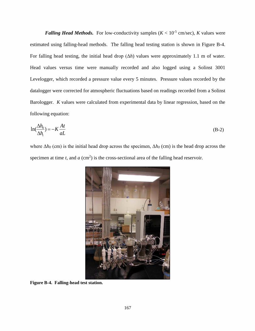
167

Falling Head Methods. For low-conductivity samples (K < 10-5 cm/sec), K values were

estimated using falling-head methods. The falling head testing station is shown in Figure B-4.

For falling head testing, the initial head drop (Δh) values were approximately 1.1 m of water.

Head values versus time were manually recorded and also logged using a Solinst 3001

Levelogger, which recorded a pressure value every 5 minutes. Pressure values recorded by the

datalogger were corrected for atmospheric fluctuations based on readings recorded from a Solinst

Barologger. K values were calculated from experimental data by linear regression, based on the

following equation:

aLAt

Khh

t

)ln( 0 (B-2)

where Δh0 (cm) is the initial head drop across the specimen, Δh0 (cm) is the head drop across the

specimen at time t, and a (cm2) is the cross-sectional area of the falling head reservoir.

Figure B-4. Falling-head test station.

168

Table B-1. Estimated foc versus depth at three locations MW38, zmw173, and MW700 MW38 MW173 MW700

Depth (ft) foc (%) Depth (ft) foc (%) Depth (ft) foc (%) Depth (ft) foc (%) 9.08 4.034% 14.08 0.072% 26.83 0.311% 9.08 0.339% 9.44 0.057% 14.44 0.110% 27.19 0.224% 9.44 0.213% 9.80 0.096% 14.80 0.105% 27.55 0.000% 9.80 0.102% 10.16 0.032% 15.16 0.029% 27.91 0.000% 10.16 0.137% 10.53 0.025% 15.53 0.038% 28.28 0.000% 10.53 0.052% 10.89 0.013% 15.89 0.065% 28.64 0.000% 10.89 0.086% 11.25 0.000% 16.98 0.000% 29.00 0.071% 11.25 0.186% 11.58 0.055% 17.31 0.000% 29.33 0.025% 11.58 0.386% 11.94 0.048% 17.64 0.000% 29.69 0.000% 11.94 0.170% 12.30 0.000% 17.97 0.007% 30.05 0.027% 12.30 0.216% 12.66 0.257% 18.29 0.068% 30.41 0.033% 12.66 0.096% 13.03 0.315% 18.62 0.079% 30.78 0.076% 13.56 0.120% 13.39 0.000% 18.95 0.011% 31.14 0.038% 13.92 0.064% 14.98 0.051% 19.28 0.047% 31.50 0.039% 14.41 0.132% 15.34 0.265% 19.41 0.095% 31.83 0.105% 14.77 0.091% 15.71 0.014% 19.77 0.049% 32.19 0.133% 15.13 0.077% 16.07 0.052% 20.14 0.075% 32.55 0.057% 15.49 0.057% 17.58 0.116% 20.50 0.036% 32.91 0.053% 15.85 0.070% 17.94 0.000% 20.86 0.044% 33.28 0.056% 16.21 0.114% 18.30 0.000% 21.22 0.032% 33.64 0.097% 16.58 0.029% 18.66 0.000% 21.41 0.036% 34.00 0.058% 16.66 0.179% 18.96 0.001% 21.83 0.075% 34.33 0.092% 16.75 0.077% 19.08 0.079% 22.19 0.052% 34.69 0.064% 16.83 0.184% 19.44 0.021% 22.55 0.031% 35.05 0.093% 16.91 0.240% 19.80 0.425% 22.91 0.000% 35.41 0.116% 16.99 0.059% 20.16 0.021% 23.28 0.000% 35.78 0.057% - - 20.53 0.000% 23.64 0.000% 36.14 0.084% - - 20.89 0.000% 24.00 0.075% 36.50 0.053% - - 21.25 0.074% 24.33 0.000% 36.83 0.054% - - 21.58 0.081% 24.69 0.090% 37.19 0.044% - - 21.94 0.144% 25.05 0.121% 37.55 0.042% - - 22.30 0.354% 25.41 0.032% 37.91 0.042% - - 22.66 0.261% 25.78 0.000% 38.28 0.049% - -

- - 26.14 0.178% 38.64 0.053% - - - - 26.50 0.074% 39.00 0.036% - -

169

APPENDIX C

SUPPORTING INFORMATION FOR SPATIAL DISTRIBUTION ANALYSIS OF NON-

AQUEOUS PHASE LIQUIDS IN POROUS MEDIA USING NUCLEAR MAGNETIC

RESONANCE: LABORATORY AND FIELD STUDIES

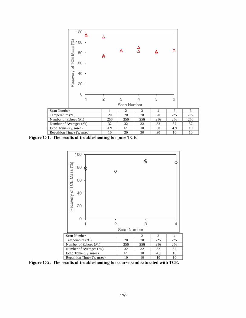
170

Scan Number 1 2 3 4 5 6 Temperature (°C) 20 20 20 20 -25 -25 Number of Echoes (NE) 256 256 256 256 256 256 Number of Averages (NA) 32 32 32 32 32 32 Echo Tome (TE, msec) 4.9 4.9 10 30 4.9 10 Repetition Time (TR, msec) 10 30 30 30 10 10

Figure C-1. The results of troubleshooting for pure TCE.

Scan Number 1 2 3 4 Temperature (°C) 20 20 -25 -25 Number of Echoes (NE) 256 256 256 256 Number of Averages (NA) 32 32 32 32 Echo Tome (TE, msec) 4.9 10 4.9 10 Repetition Time (TR, msec) 10 10 10 10

Figure C-2. The results of troubleshooting for coarse sand saturated with TCE.

171

Scan Number 1 2 3 4 5 6 Temperature (°C) 20 20 -25 -25 -25 -25 Number of Echoes (NE) 256 256 256 256 256 256 Number of Averages (NA) 32 32 32 32 32 32 Echo Tome (TE, msec) 4.9 10 4.9 10 4.9 10 Repetition Time (TR, msec) 10 10 10 10 30 30

Figure C-3. The results of troubleshooting for fine sand saturated with TCE.

Scan Number 1 2 3 Temperature (°C) 20 20 -25 Number of Echoes (NE) 256 256 256 Number of Averages (NA) 32 32 32 Echo Tome (TE, msec) 4.9 10 4.9 Repetition Time (TR, msec) 10 10 10

Figure C-4. The results of troubleshooting for coarse glass beads saturated with TCE.

172

Scan Number 1 2 3 Temperature (°C) 20 20 -25 Number of Echoes (NE) 256 256 256 Number of Averages (NA) 32 32 32 Echo Tome (TE, msec) 4.9 10 4.9 Repetition Time (TR, msec) 20 30 10

Figure C-5. The results of troubleshooting for fine glass beads saturated with TCE.

Figure C-6. The results of downhole NMR logging at MLSTE#2: a) T2 distribution versus depth and b) water content versus depth.

173

Figure C-7. The results of downhole NMR logging at SS-26D: a) T2 distribution versus depth and b) water content versus depth.

Figure C-8. Measured NMR logging data at SS-115 from a) short- and b) long-echo times.

174

APPENDIX D

SUPPORTING INFORMATION FOR MONITORING DEPLETION OF LIGHT NON-

AQUEOUS PHASE LIQUID IN SHALLOW GEOLOGICAL FORMATIONS USING

ELECTRICAL RESISTIVITY

175

Table D-1. Measured data at MLSTE#1 on 11/6/2013 Depth (foot)

ρ (Ω∙m)

Temperature (°C)

pH ORP (mV)

Ca Mg Na K Br CO3 HCO3 Cl SO4 Hardness as CaCO3

Alkalinity as CaCO3

TDS Fe Mn ρf

(Ω∙m) (mg/L)

1 - - - - - - - - - - - - - - - - - - - 2 - - - - - - - - - - - - - - - - - - - 3 161,827 6.4 - - - - - - - - - - - - - - - - - 4 254,825 8.1 - - - - - - - - - - - - - - - - - 5 547,723 9.6 - - - - - - - - - - - - - - - - - 6 464,990 11.4 - - - - - - - - - - - - - - - - - 7 92,270 12.6 - - - - - - - - - - - - - - - - - 8 34,395 12.7 - - - - - - - - - - - - - - - - - 9 4,087 13.6 - - - - - - - - - - - - - - - - - 10 1,096 13.6 7.03 28 66.5 151 561 15.4 1.8 10.5 403 10.0 1599 788 348 2,818 0.57 1.10 2.47 11 529 14.3 7.07 20.7 65.9 159 582 15.7 1.7 9.8 449 10.8 1637 818 384 2,930 0.16 0.95 2.38 12 572 14.4 7.06 39.6 55.4 139 570 11.8 1.5 10.7 422 9.5 1523 709 364 2,743 0.09 0.17 2.55 13 615 14 7.03 27.8 61.7 143 587 11.2 1.7 11.3 402 10.3 1601 741 348 2,829 0.10 0.42 2.47 14 602 14.1 7.06 22.1 72.1 177 669 13.2 2.0 10.4 550 11.3 1817 907 468 3,322 0.10 0.21 2.11


ρ (Ω∙m)

Temperature (°C)

pH ORP (mV)


Alkalinity as CaCO3

TDS Fe Mn ρf

(Ω∙m) (mg/L)

0 - - - - - - - - - - - - - - - - - - 1 - - - - - - - - - - - - - - - - - - 2 - - - - - - - - - - - - - - - - - - 3 283,743 3.3 - - - - - - - - - - - - - - - - - 4 545,999 3.7 - - - - - - - - - - - - - - - - - 5 581,697 4.1 - - - - - - - - - - - - - - - - - 6 357,131 5.7 - - - - - - - - - - - - - - - - - 7 168,990 6.4 - - - - - - - - - - - - - - - - - 8 39,490 6.8 - - - - - - - - - - - - - - - - - 9 4,635 7.5 - - - - - - - - - - - - - - - - - 10 1,157 7.9 7.59 -49 - - - - - - - - - - - - - - - 11 634 8.5 6.58 -3 - - - - - - - - - - - - - - - 12 687 9.6 7.55 -20 - - - - - - - - - - - - - - - 13 727 9.2 7.48 -8 - - - - - - - - - - - - - - - 14 704 9.6 7.45 -2 - - - - - - - - - - - - - - -

176


ρ (Ω∙m)

Temperature (°C)

pH ORP (mV)


Alkalinity as CaCO3

TDS Fe Mn ρf

(Ω∙m) (mg/L)

0 - - - - - - - - - - - - - - - - - - - 1 - - - - - - - - - - - - - - - - - - - 2 - - - - - - - - - - - - - - - - - - - 3 30,523 13.9 - - - - - - - - - - - - - - - - - 4 55,190 12.1 - - - - - - - - - - - - - - - - - 5 69,000 11 - - - - - - - - - - - - - - - - - 6 60,360 10 - - - - - - - - - - - - - - - - - 7 32,150 9.7 - - - - - - - - - - - - - - - - - 8 8,495 9.3 - - - - - - - - - - - - - - - - - 9 1,183 9.1 - - - - - - - - - - - - - - - - - 10 363 9.1 7.44 -67 - - - - - - - - - - - - - - - 11 162 9.2 7.37 -39 - - - - - - - - - - - - - - - 12 176 8.9 7.34 -31 - - - - - - - - - - - - - - - 13 186 9.1 7.33 -22 - - - - - - - - - - - - - - - 14 181 9.1 7.31 -19 - - - - - - - - - - - - - - -


ρ (Ω∙m)

Temperature (°C)

pH ORP (mV)


Alkalinity as CaCO3

TDS Fe Mn ρf

(Ω∙m) (mg/L)

0 - - - - - - - - - - - - - - - - - - - 1 - - - - - - - - - - - - - - - - - - - 2 - - - - - - - - - - - - - - - - - - - 3 151,984 24.1 - - - - - - - - - - - - - - - - - 4 235,176 23.5 - - - - - - - - - - - - - - - - - 5 190,822 22.7 - - - - - - - - - - - - - - - - - 6 86,640 21.1 - - - - - - - - - - - - - - - - - 7 31,626 19.5 - - - - - - - - - - - - - - - - - 8 3,960 18.7 - - - - - - - - - - - - - - - - - 9 986 17.3 - - 238 176 642 7.31 0.01 - - 103 1457 - 865 2550 - - 1.83 10 865 16.1 - - 121 162 587 6.18 0.01 - - 110 1504 - 944 2656 - - 2.21 11 527 16.1 - - 270 207 668 7.33 0.01 - - 220 2117 - 657 3565 - - 1.67 12 562 15.1 - - 271 200 672 7.31 0.01 - - 171 1850 - 889 3208 - - 1.68 13 613 14.7 - - 285 211 750 8.04 0.01 - - 132 1973 - 952 3352 - - 1.55 14 604 14.4 - - 243 176 734 13.2 0.01 - - 137 1810 - 1117 3218 - - 1.69

177


ρ (Ω∙m)

Temperature (°C)

pH ORP (mV)


Alkalinity as CaCO3

TDS Fe Mn ρf

(Ω∙m) (mg/L)

0 - - - - - - - - - - - - - - - - - - - 1 - - - - - - - - - - - - - - - - - - - 2 - - - - - - - - - - - - - - - - - - - 3 29,100 17.3 - - - - - - - - - - - - - - - - - 4 49,670 17.2 - - - - - - - - - - - - - - - - - 5 38,900 16.6 - - - - - - - - - - - - - - - - - 6 19,130 16.1 - - - - - - - - - - - - - - - - - 7 7,280 15.7 - - - - - - - - - - - - - - - - - 8 2,900 15.5 - - - - - - - - - - - - - - - - - 9 1,280 15.2 351 254 982 26.8 0.01 0 0 107 1563 1.59 351 - - 6118 - - 1.22 10 476 15.1 385 277 1057 28.9 0.01 0 0 120 1633 2.17 385 - - 6647 - - 1.12 11 137 14.5 398 271 1076 28.8 0.01 0 0 116 1620 1.9 398 - - 6739 - - 1.11 12 150 14.2 400 274 1069 29.1 0.01 0 0 132 1723 1.06 400 - - 6701 - - 1.11 13 161 13.8 429 351 1203 31.9 0.01 0 0 169 1955 0.93 429 - - 7693 - - 0.96 14 154 14 433 302 1325 50.3 0.01 0 0 142 1924 1.11 433 - - 7932 - - 0.95


ρ (Ω∙m)

Temperature (°C)

pH ORP (mV)


Alkalinity as CaCO3

TDS Fe Mn ρf

(Ω∙m) (mg/L)

0 - - - - - - - - - - - - - - - - - - - 1 - - - - - - - - - - - - - - - - - - - 2 - - - - - - - - - - - - - - - - - - - 3 45,120 8.2 - - - - - - - - - - - - - - - - - 4 24,552 10.5 - - - - - - - - - - - - - - - - - 5 4,405 11.4 - - - - - - - - - - - - - - - - - 6 4,022 12.6 - - - - - - - - - - - - - - - - - 7 3,518 13.8 - - - - - - - - - - - - - - - - - 8 2,350 14.4 - - - - - - - - - - - - - - - - - 9 1,566 15.1 7.6 -170 18.0 21.6 15.8 2.8 1.4 12.7 177.0 0.8 4.1 134.0 166.0 254.0 4.1 2.5 28.91 10 1,852 15.8 6.6 -183 32.5 18.5 15.5 2.2 1.2 8.9 212.0 0.6 4.5 157.0 188.0 295.0 1.8 2.4 25.66 11 2,055 16.7 6.6 -211 27.4 20.4 17.9 2.4 1.5 8.8 209.0 0.5 7.0 152.0 186.0 295.0 0.6 2.0 25.58 12 1,442 17.2 6.5 -291 10.3 59.8 95.5 3.7 1.4 14.7 508.0 1.6 39.4 272.0 441.0 734.0 0.2 1.9 10.26 13 763 18.0 7.2 -293 11.0 97.0 171.0 4.0 1.3 18.4 716.0 5.3 171.0 427.0 617.0 1194.0 0.1 1.0 6.18 14 691 17.8 7.0 -257 11.8 103.0 194.0 3.9 2.6 18.3 617.0 3.2 325.0 452.0 537.0 1279.0 0.3 0.5 5.65

178


ρ (Ω∙m)

Temperature (°C)

pH ORP (mV)


Alkalinity as CaCO3

TDS Fe Mn ρf

(Ω∙m) (mg/L)

0 - - - - - - - - - - - - - - - - - - - 1 - - - - - - - - - - - - - - - - - - - 2 - - - - - - - - - - - - - - - - - - - 3 31,569 7.7 - - - - - - - - - - - - - - - - - 4 16,991 7.7 - - - - - - - - - - - - - - - - - 5 4,336 8.0 - - - - - - - - - - - - - - - - - 6 3,525 8.4 - - - - - - - - - - - - - - - - - 7 3,505 9.3 - - - - - - - - - - - - - - - - - 8 2,315 9.9 - - - - - - - - - - - - - - - - - 9 1,437 9.8 7.1 -118 - - - - - - - - - - - - - - - 10 1,663 10.6 7.1 -113 - - - - - - - - - - - - - - - 11 1,797 11.1 7.0 -133 - - - - - - - - - - - - - - - 12 1,747 11.7 6.8 -106 - - - - - - - - - - - - - - - 13 1,296 13.5 7.0 -252 - - - - - - - - - - - - - - - 14 767 12.9 7.4 -259 - - - - - - - - - - - - - - -


ρ (Ω∙m)

Temperature (°C)

pH ORP (mV)


Alkalinity as CaCO3

TDS Fe Mn ρf

(Ω∙m) (mg/L)

0 - - - - - - - - - - - - - - - - - - - 1 - - - - - - - - - - - - - - - - - - - 2 - - - - - - - - - - - - - - - - - - - 3 6,925 14.3 - - - - - - - - - - - - - - - - - 4 4,000 13.2 - - - - - - - - - - - - - - - - - 5 2,500 12.5 - - - - - - - - - - - - - - - - - 6 1,301 12.0 - - - - - - - - - - - - - - - - - 7 929 12.5 - - - - - - - - - - - - - - - - - 8 602 12.1 - - - - - - - - - - - - - - - - - 9 314 12.3 6.7 -222 - - - - - - - - - - - - - - - 10 350 12.5 6.7 -216 - - - - - - - - - - - - - - - 11 350 12.7 6.7 -247 - - - - - - - - - - - - - - - 12 278 12.8 7.1 -249 - - - - - - - - - - - - - - - 13 212 13.0 7.2 -298 - - - - - - - - - - - - - - - 14 201 12.9 7.3 -263 - - - - - - - - - - - - - - -

179


ρ (Ω∙m)

Temperature (°C)

pH ORP (mV)


Alkalinity as CaCO3

TDS Fe Mn ρf

(Ω∙m) (mg/L)

0 - - - - - - - - - - - - - - - - - - - 1 - - - - - - - - - - - - - - - - - - - 2 - - - - - - - - - - - - - - - - - - - 3 15,283 23.1 - - - - - - - - - - - - - - - - - 4 11,299 22.0 - - - - - - - - - - - - - - - - - 5 4,826 21.8 - - - - - - - - - - - - - - - - - 6 3,172 21.6 - - - - - - - - - - - - - - - - - 7 2,842 20.8 - - - - - - - - - - - - - - - - - 8 1,792 20.6 - - - - - - - - - - - - - - - - - 9 1,404 20.2 6.9 115.0 115.0 17.0 24.2 2.6 - - - 7.4 15.2 - - 177.0 - - 12.07 10 1,662 19.7 7.0 117.0 117.0 18.0 21.0 2.5 - - - 7.6 14.2 - - 189.0 - - 12.01 11 1,767 19.6 7.0 116.0 116.0 21.1 22.4 2.4 - - - 7.2 10.0 - - 180.0 - - 11.63 12 1,907 19.1 6.9 108.0 108.0 18.6 23.8 2.2 - - - 7.4 9.2 - - 168.0 - - 12.44 13 1,953 19.3 6.9 110.0 110.0 18.7 21.7 2.0 - - - 7.4 6.7 - - 173.0 - - 12.42 14 1,336 17.2 7.1 106.0 106.0 59.0 72.8 2.1 - - - 13.3 0.0 - - 246.0 - - 7.44


ρ (Ω∙m)

Temperature (°C)

pH ORP (mV)


Alkalinity as CaCO3

TDS Fe Mn ρf

(Ω∙m) (mg/L)

0 - - - - - - - - - - - - - - - - - - - 1 - - - - - - - - - - - - - - - - - - - 2 - - - - - - - - - - - - - - - - - - - 3 5,298 19.4 - - - - - - - - - - - - - - - - - 4 4,599 20.1 - - - - - - - - - - - - - - - - - 5 2,120 20.0 - - - - - - - - - - - - - - - - - 6 735 20.0 - - - - - - - - - - - - - - - - - 7 640 19.7 - - - - - - - - - - - - - - - - - 8 414 19.7 - - - - - - - - - - - - - - - - - 9 311 19.5 - - - - - - - - - - - - - - - - - 10 370 19.3 6.7 -116.3 47.1 52.2 5.1 0.0 0.0 0.0 8.3 9.8 1.4 - - 1482.0 - - 5.35 11 394 19.3 6.7 -126.0 49.5 45.2 5.0 0.0 0.0 0.0 7.6 3.7 1.4 - - 1379.0 - - 5.74 12 413 19.7 6.7 -135.0 49.2 47.0 5.0 0.0 0.0 0.0 7.8 0.0 1.4 - - 1429.0 - - 5.55 13 359 18.7 6.7 -136.6 44.9 48.2 4.3 0.0 0.0 0.0 9.4 3.5 1.5 - - 1303.0 - - 6.08 14 221 18.1 7.2 -269.5 211.0 277.0 11.2 0.0 0.0 0.0 65.2 3.1 0.7 - - 3781.0 - - 2.01

dissertation third-generation site characterization

Documents