dirichlet process mixture models for modeling and ... · modeling and generating synthetic versions...
TRANSCRIPT
Vol. 00 (0000) 1DOI: 0000
Dirichlet Process Mixture Models for
Modeling and Generating Synthetic
Versions of Nested Categorical Data
Jingchen Hu1,∗,?? , Jerome P. Reiter2,∗,†,??,?? and Quanli Wang2,†,??
1Department of Mathematics and Statistics, Vassar College, Box 27, Poughkeepsie, NY12604 e-mail: [email protected]
2Department of Statistical Science, Duke University, Durham, NC 27708-0251 e-mail:[email protected]
3Department of Statistical Science, Duke University, Durham, NC 27708-0251 e-mail:[email protected]
Abstract:We present a Bayesian model for estimating the joint distribution of
multivariate categorical data when units are nested within groups. Suchdata arise frequently in social science settings, for example, people livingin households. The model assumes that (i) each group is a member of agroup-level latent class, and (ii) each unit is a member of a unit-level latentclass nested within its group-level latent class. This structure allows themodel to capture dependence among units in the same group. It also fa-cilitates simultaneous modeling of variables at both group and unit levels.We develop a version of the model that assigns zero probability to groupsand units with physically impossible combinations of variables. We applythe model to estimate multivariate relationships in a subset of the Ameri-can Community Survey. Using the estimated model, we generate synthetichousehold data that could be disseminated as redacted public use files.Supplementary materials for this article are available online.
Keywords and phrases: Confidentiality, Disclosure, Latent, Multino-mial, Synthetic.
1. Introduction
In many settings, the data comprise units nested within groups (e.g., peoplewithin households), and include categorical variables measured at the unit level(e.g., individuals’ demographic characteristics) and at the group level (e.g.,whether the family owns or rents their home). A typical analysis goal is toestimate multivariate relationships among the categorical variables, accountingfor the hierarchical structure in the data.
To estimate joint distributions with multivariate categorical data, many an-alysts rely on mixtures of products of multinomial distributions, also known as
∗National Science Foundation CNS-10-12141†National Science Foundation SES-11-31897‡Arthur P. Sloan Foundation G-2015-2-166003
1
imsart-generic ver. 2011/11/15 file: arxiv_version_3.tex date: November 1, 2016
arX
iv:1
412.
2282
v6 [
stat
.ME
] 2
8 O
ct 2
016
J. Hu et al./ 2
latent class models. These models assume that each unit is a member of an unob-served cluster, and that variables follow independent multinomial distributionswithin clusters. Latent class models can be estimated via maximum likelihood(Goodman, 1974) and Bayesian approaches (Ishwaran and James, 2001; Jainand Neal, 2007; Dunson and Xing, 2009). Of particular note, Dunson and Xing(2009) present a nonparametric Bayesian version of the latent class model, usinga Dirichlet process mixture (DPM) for the prior distribution. The DPM priordistribution is appealing, in that (i) it has full support on the space of joint dis-tributions for unordered categorical variables, ensuring that the model does notrestrict dependence structures a priori, and (ii) it fully incorporates uncertaintyabout the effective number of latent classes in posterior inferences.
For data nested within groups, however, standard latent class models maynot offer accurate estimates of joint distributions. In particular, it may not beappropriate to treat the units in the same group as independent; for example, de-mographic variables like age, race, and sex of individuals in the same householdare clearly dependent. Similarly, some combinations of units may be physicallyimpossible to place in the same group, such as a daughter who is older than herbiological father. Additionally, every unit in a group must have the same valuesof group-level variables, so that one cannot simply add multinomial kernels forthe group-level variables.
In this article, we present a Bayesian mixture model for nested categoricaldata. The model assumes that (i) each group is a member of a group-level latentclass, and (ii) each unit is a member of a unit-level latent class nested within itsgroup-level latent class. This structure encourages the model to cluster groupsinto data-driven types, for example, households with children where everyonehas the same race. This in turn allows for dependence among units in the samegroup. The nested structure also facilitates simultaneous modeling of variablesat both group and unit levels. We refer to the model as the nested data Dirich-let process mixture of products of multinomial distributions (NDPMPM). Wepresent two versions of the NDPMPM: one that gives support to all configu-rations of groups and units, and one that assigns zero probability to groupsand units with physically impossible combinations of variables (also known asstructural zeros in the categorical data analysis literature).
The NDPMPM is similar to the latent class models proposed by Vermunt(2003, 2008), who also uses two layers of latent classes to model nested categor-ical data. These models use a fixed number of classes as determined by a modelselection criterion (e.g., AIC or BIC), whereas the NDPMPM allows uncertaintyin the effective number of classes at each level. The NDPMPM also is similarto the latent class models in Bennink et al. (2016) for nested data, especiallyto what they call the “indirect model.” The indirect model regresses a singlegroup-level outcome on group-level and individual-level predictors, whereas theNDPMPM is used for estimation of the joint distribution of multiple group-leveland individual-level variables. To the best of our knowledge, the models of Ver-munt (2003, 2008) and Bennink et al. (2016) do not account for groups withphysically impossible combinations of units.
One of our primary motivations in developing the NDPMPM is to develop
imsart-generic ver. 2011/11/15 file: arxiv_version_3.tex date: November 1, 2016

J. Hu et al./ 3
a method for generating redacted public use files for household data, specifi-cally for the variables on the United States decennial census. Public use files inwhich confidential data values are replaced with draws from predictive distri-butions are known in the disclosure limitation literature as synthetic datasets(Rubin, 1993; Little, 1993; Raghunathan et al., 2003; Reiter, 2005; Reiter andRaghunathan, 2007). Synthetic data techniques have been used to create severalhigh-profile public use data products, including the Survey of Income and Pro-gram Participation (Abowd et al., 2006), the Longitudinal Business Database(Kinney et al., 2011), the American Community Survey group quarters data(Hawala, 2008), and the OnTheMap application (Machanavajjhala et al., 2008).None of these products involve synthetic household data. In these products, thesynthesis strategies are based on chains of generalized linear models for indepen-dent individuals, e.g., simulate variable x1 from some parametric model f(x1),x2 from some parametric model f(x2|x1), etc. We are not aware of any syn-thesis models appropriate for nested categorical data like the decennial censusvariables.
As part of generating the synthetic data, we evaluate disclosure risks usingthe measures suggested in Hu et al. (2014). Specifically, we quantify the posteriorprobabilities that intruders can learn values from the confidential data given thereleased synthetic data, under assumptions about the intruders’ knowledge andattack strategy. This is the only strategy we know of for evaluating statisticaldisclosure risks for nested categorical data. To save space, the methodology andresults for the disclosure risk evaluations are presented in the supplementarymaterial only. To summarize very briefly, the analyses suggest that syntheticdata generated from the NDPMPM have low disclosure risks.
The remainder of this article is organized as follows. In Section 2, we presentthe NDPMPM model when all configurations of groups and units are feasible.In Section 3, we present a data augmentation strategy for estimating a versionof the NDPMPM that puts zero probability on impossible combinations. InSection 4, we illustrate and evaluate the NDPMPM models using householddemographic data from the American Community Survey (ACS). In particular,we use posterior predictive distributions from the NDPMPM models to generatesynthetic datasets, and compare results of representative analyses done withthe synthetic and original data. In Section 5, we conclude with discussion ofimplementation of the proposed models.
2. The NDPMPM Model
As a working example, we suppose the data include N individuals residing inonly one of n < N households, where n (but not N) is fixed by design. Fori = 1, . . . , n, let ni ≥ 1 equal the number of individuals in house i, so that∑ni=1 ni = N . For k = 1, . . . , p, let Xijk ∈ {1, . . . , dk} be the value of categorical
variable k for person j in household i, where i = 1, . . . , n and j = 1, . . . , ni. Fork = p+1, . . . , p+q, let Xik ∈ {1, . . . , dk} be the value of categorical variable k forhousehold i, which is assumed to be identical for all ni individuals in household
imsart-generic ver. 2011/11/15 file: arxiv_version_3.tex date: November 1, 2016

J. Hu et al./ 4
i. We let one of the variables in Xik correspond to the household size ni; thus,N is a random variable. For now, we assume no impossible combinations ofvariables within individuals or households.
We assume that each household belongs to some group-level latent class,which we label with Gi, where i = 1, . . . , n. Let πg = Pr(Gi = g) for any classg; that is, πg is the probability that household i belongs to class g for everyhousehold. For any k ∈ {p + 1, . . . , p + q} and any value c ∈ {1, . . . , dk}, let
λ(k)gc = Pr(Xik = c | Gi = g) for any class g; here, λ
(k)gc is the same value
for every household in class g. For computational expediency, we truncate thenumber of group-level latent classes at some sufficiently large value F . Let π =
{π1, . . . , πF }, and let λ = {λ(k)gc : c = 1, . . . , dk; k = p+1, . . . , p+q; g = 1, . . . , F}.Within each household class, we assume that each individual member belongs
to some individual-level latent class, which we label with Mij , where i = 1, . . . , nand j = 1, . . . , ni. Let ωgm = Pr(Mij = m | Gi = g) for any class (g,m); thatis, ωgm is the conditional probability that individual j in household i belongs toindividual-level class m nested within group-level class g, for every individual.
For any k ∈ {1, . . . , p} and any value c ∈ {1, . . . , dk}, let φ(k)gmc = Pr(Xijk =
c | (Gi,Mij) = (g,m)); here, φ(k)gmc is the same value for every individual in
class (g,m). Again for computational expediency, we truncate the number ofindividual-level latent classes within each g at some sufficiently large number Sthat is common across all g. Thus, the truncation results in a total of F × Slatent classes used in computation. Let ω = {ωgm : g = 1, . . . , F ;m = 1, . . . , S},and let φ = {φ(k)gmc : c = 1, . . . , dk; k = 1, . . . , p; g = 1, . . . , F ;m = 1, . . . , S}.
We let both the q household-level variables and p individual-level variablesfollow independent, class-specific multinomial distributions. Thus, the model forthe data and corresponding latent classes in the NDPMPM is
Xik | Gi, λ ∼ Multinomial(λ(k)Gi1
, . . . , λ(k)Gidk
)
for all i, k = p+ 1, . . . , p+ q (1)
Xijk | Gi,Mij , ni, φ ∼ Multinomial(φ(k)GiMij1
, . . . , φ(k)GiMijdk
)
for all i, j, k = 1, . . . , p (2)
Gi | π ∼ Multinomial(π1, . . . , πF ) for all i, (3)
Mij | Gi, ni, ω ∼ Multinomial(ωGi1, . . . , ωGiS) for all i, j, (4)
where each multinomial distribution has sample size equal to one and num-ber of levels implied by the dimension of the corresponding probability vector.We allow the multinomial probabilities for individual-level classes to differ byhousehold-level class. One could impose additional structure on the probabili-ties, for example, force them to be equal across classes as suggested in Vermunt(2003, 2008); we do not pursue such generalizations here.
We condition on ni in (2) and (4) so that the entire model can be interpretedas a generative model for households; that is, the size of the household could besampled from (1), and once the size is known the characteristics of the house-hold’s individuals could be sampled from (2). The distributions in (2) and (4)
imsart-generic ver. 2011/11/15 file: arxiv_version_3.tex date: November 1, 2016
J. Hu et al./ 5
do not depend on ni other than to fix the number of people in the household;that is, within any Gi, the distributions of all parameters do not depend on ni.This encourages borrowing strength across households of different sizes whilesimplifying computations.
As prior distributions on π and ω, we use the truncated stick breaking rep-resentation of the Dirichlet process (Sethuraman, 1994). We have
πg = ug∏f<g
(1− uf ) for g = 1, . . . , F (5)
ug ∼ Beta(1, α) for g = 1, . . . , F − 1, uF = 1 (6)
α ∼ Gamma(aα, bα) (7)
ωgm = vgm∏s<m
(1− vgs) for m = 1, . . . , S (8)
vgm ∼ Beta(1, βg) for m = 1, . . . , S − 1, vgS = 1 (9)
βg ∼ Gamma(aβ , bβ). (10)
The prior distribution in (5)–(10) is similar to the truncated version of the nestedDirichlet process prior distribution of Rodriguez et al. (2008) based on condi-tionally conjugate prior distributions (see Section 5.1 in their article). The priordistribution in (5)–(10) also shares characteristics with the enriched Dirichletprocess prior distribution of Wade et al. (2011), in that (i) it gets around thelimitations caused by using a single precision parameter α for the mixture prob-abilities, and (ii) it allows different mixture components for different variables.
As prior distributions on λ and φ, we use independent Dirichlet distributions,
λ(k)g = (λ(k)g1 , . . . , λ
(k)gdk
) ∼ Dir(ak1, . . . , akdk) (11)
φ(k)gm = (φ(k)gm1, . . . , φ
(k)gmdk
) ∼ Dir(ak1, . . . , akdk). (12)
One can use data-dependent prior distributions for setting each (ak1, . . . , akdk ),for example, set it equal to the empirical marginal frequency. Alternatively, onecan set ak1 = · · · = akdk = 1 for all k to correspond to uniform distributions.We examined both approaches and found no practical differences between themfor our applications; see the supplementary material. In the applications, wepresent results based on the empirical marginal frequencies. Following Dunsonand Xing (2009) and Si and Reiter (2013), we set (aα = .25, bα = .25) and(aβ = .25, bβ = .25), which represents a small prior sample size and hence vaguespecification for the Gamma distributions. We estimate the posterior distribu-tion of all parameters using a blocked Gibbs sampler (Ishwaran and James,2001; Si and Reiter, 2013); see the supplement for the relevant full conditionals.
Intuitively, the NDPMPM seeks to cluster households with similar compo-sitions. Within the pool of individuals in any household-level class, the modelseeks to cluster individuals with similar characteristics. Because individual-levellatent class assignments are conditional on household-level latent class assign-ments, the model induces dependence among individuals in the same house-hold (more accurately, among individuals in the same household-level cluster).
imsart-generic ver. 2011/11/15 file: arxiv_version_3.tex date: November 1, 2016

J. Hu et al./ 6
To see this mathematically, consider the expression for the joint distributionfor variable k for two individuals j and j′ in the same household i. For any(c, c′) ∈ {1, . . . , dk}, we have
Pr(Xijk = c,Xij′k = c′) =
F∑g=1
(S∑
m=1
φ(k)gmcωgm
S∑m=1
φ(k)gmc′ωgm
)πg. (13)
Since Pr(Xijk = c) =∑Fg=1
∑Sm=1 φ
(k)gmcωgmπg for any c ∈ {1, . . . , dk}, the
Pr(Xijk = c,Xij′k = c′) 6= Pr(Xijk = c)Pr(Xij′k = c′).Ideally we fit enough latent classes to capture key features in the data while
keeping computations as expedient as possible. As a strategy for doing so, wehave found it convenient to start an MCMC chain with reasonably-sized valuesof F and S, say F = S = 10. After convergence of the MCMC chain, we checkhow many latent classes at the household-level and individual-level are occupiedacross the MCMC iterations. When the numbers of occupied household-levelclasses hits F , we increase F . When this is not the case but the number of occu-pied individual-level classes hits S, we try increasing F alone, as the increasednumber of household-level latent classes may sufficiently capture heterogeneityacross households as to make S adequate. When increasing F does not help,for example there are too many different types of individuals, we increase S,possibly in addition to F . We emphasize that these types of titrations are usefulprimarily to reduce computation time; analysts always can set S and F both tobe very large so that they are highly likely to exceed the number of occupiedclasses in initial runs.
It is computationally convenient to set βg = β for all g in (10), as doing soreduces the number of parameters in the model. Allowing βg to be class-specificoffers additional flexibility, as the prior distribution of the household-level classprobabilities can vary by class. In our evaluations of the model on the ACS data,results were similar whether we used a common or distinct values of βg.
3. Adapting the NDPMPM for Impossible Combinations
The models in Section 2 make no restrictions on the compositions of groups orindividuals. In many contexts this is unrealistic. Using our working example,suppose that the data include a variable that characterizes relationships amongindividuals in the household, as the ACS does. Levels of this variable includehousehold head, spouse of household head, parent of the household head, etc.By definition, each household must contain exactly one household head. Addi-tionally, by definition (in the ACS), each household head must be at least 15years old. Thus, we require a version of the NDPMPM that enforces zero prob-ability for any household that has zero or multiple household heads, and anyhousehold headed by someone younger than 15 years.
We need to modify the likelihoods in (1) and (2) to enforce zero probability forimpossible combinations. Equivalently, we need to truncate the support of theNDPMPM. To express this mathematically, let Ch represent all combinations of
imsart-generic ver. 2011/11/15 file: arxiv_version_3.tex date: November 1, 2016
J. Hu et al./ 7
individuals and households of size h, including impossible combinations; that is,Ch is the Cartesian product Πp+q
k=p+1(1, . . . , dk)(Πhj=1Πp
k=1(1, . . . , dk)). For any
household with h individuals, let Sh ⊂ Ch be the set of combinations that shouldhave zero probability, i.e., Pr(Xip+1, . . . , Xip+q, Xi11, . . . , Xihp ∈ Sh) = 0. LetC =
⋃h∈H Ch and S =
⋃h∈H Sh, where H is the set of all household sizes
in the observed data. We define a random variable for all the data for personj in household i as X∗ij = (X∗ij1, . . . , X
∗ijp, X
∗ip+1, . . . , X
∗ip+q), and a random
variable for all data in household i as X∗i = (X∗i1, . . . ,X∗ini
). Here, we writea superscript ∗ to indicate that the random variables have support only onC − S; in contrast, we use Xij and Xi to indicate the corresponding randomvariables with unrestricted support on C. Letting X ∗ be the sampled data fromn households, i.e., a realization of (X∗1, . . . ,X
∗n), the likelihood component of
the truncated NDPMPM model, p(X ∗|θ), can be written as proportional toL(X ∗ | θ) =
n∏i=1
∑h∈H
1{ni = h}1{X∗i /∈ Sh}F∑g=1
p+q∏k=p+1
λ(k)gX∗
ik
h∏j=1
S∑m=1
p∏k=1
φ(k)gmX∗
ijkωgm
πg
(14)
where θ includes all parameters of the model described in Section 2. Here, 1{.}equals one when the condition inside the {} is true and equals zero otherwise.
For all h ∈ H, let n∗h =∑ni=1 1{ni = h} be the number of households of
size h in X ∗. Let π0h(θ) = Pr(Xi ∈ Sh|θ), where Xi is the random variablewith unrestricted support. The normalizing constant in the likelihood in (14) is∏h∈H(1− π0h(θ))n∗h . Hence, we seek to compute the posterior distribution
p(θ|X ∗, T (S)) ∝ p(X ∗ | θ)p(θ) =1∏
h∈H(1− π0h(θ))n∗hL(X ∗ | θ)p(θ). (15)
The T (S) emphasizes that the density is for the truncated NDPMPM, not thedensity from Section 2.
The Gibbs sampling strategy from Section 2 requires conditional indepen-dence across individuals and variables, and hence unfortunately is not appro-priate as a means to estimate the posterior distribution. Instead, we follow thegeneral approach of Manrique-Vallier and Reiter (2014). The basic idea is totreat the observed data X ∗, which we assume includes only feasible householdsand individuals (e.g., there are no reporting errors that create impossible com-binations in the observed data), as a sample from an augmented dataset X ofunknown size. We assume X arises from an NDPMPM model that does not re-strict the characteristics of households or individuals; that is, all combinationsof households and individuals are allowable in the augmented sample. With thisconceptualization, we can construct a Gibbs sampler that appropriately assignszero probability to combinations in S and results in draws of θ from (15). Givena draw of θ, we draw X using a negative binomial sampling scheme. For eachstratum h ∈ H defined by unique household sizes in X ∗, we repeatedly simulatehouseholds with individuals from the untruncated NDPMPM model, stoppingwhen the number of simulated feasible households matches n∗h. We make X
imsart-generic ver. 2011/11/15 file: arxiv_version_3.tex date: November 1, 2016

J. Hu et al./ 8
comprise X ∗ and the generated households that fall in S. Given a draw of X ,we draw θ from the NDPMPM model as in Section 2, treating X as if it werecollected data. The full conditionals for this sampler, as well as a proof that itgenerates draws from (15), are provided in the supplement.
4. Using the NDPMPM to Generate Synthetic Household Data
We now illustrate the ability of the NDPMPM to estimate joint distributionsfor subsets of household level and individual level variables. Section 4.1 presentsresults for a scenario where the variables are free of structural zeros (i.e., S = ∅),and Section 4.2 presents results for a scenario with impossible combinations.
We use subsets of variables selected from the public use files for the ACS.As brief background, the purpose of the ACS is to enable estimation of popula-tion demographics and housing characteristics for the entire United States. Thequestionnaire is sent to about 1 in 38 households. It includes questions about theindividuals living in the household (e.g., their ages, races, incomes) and aboutthe characteristics of the housing unit (e.g., number of bedrooms, presence ofrunning water or not, presence of a telephone line or not). We use only datafrom non-vacant households.
In both simulation scenarios, we treat data from the public use files as popu-lations, so as to have known population values, and take simple random samplesfrom them on which we estimate the NDPMPM models. We use the estimatedposterior predictive distributions to create simulated versions of the data, andcompare analyses of the simulated data to the corresponding analyses based onthe observed data and the constructed population values.
If we act like the samples from the constructed populations are confidentialand cannot be shared as is, the simulated datasets can be viewed as redactedpublic use file, i.e., synthetic data. We generate L synthetic datasets, Z =(Z(1), . . . ,Z(L)), by sampling L datasets from the posterior predictive distri-bution of a NDPMPM model. We generate synthetic data so that the numberof households of any size h in each Z(l) exactly matches n∗h. This improves thequality of the synthetic data by ensuring that the total number of individualsand household size distributions match in Z and X ∗. As a result, Z comprisespartially synthetic data (Little, 1993; Reiter, 2003), even though every releasedZijk is a simulated value.
To make inferences with Z we use the approach in Reiter (2003). Supposethat we seek to estimate some scalar quantity Q. For l = 1, . . . , L, let q(l) andu(l) be respectively the point estimate of Q and its associated variance estimatecomputed with Z(l). Let qL =
∑l q
(l)/L; uL =∑l u
(l)/L; bL =∑l(q
(l) −qL)2/(L − 1); and TL = uL + bL/L. We make inferences about Q using thet−distribution, (qL −Q) ∼ tv(0, TL), with v = (L− 1)(1 +LuL/bL)2 degrees offreedom.
imsart-generic ver. 2011/11/15 file: arxiv_version_3.tex date: November 1, 2016
J. Hu et al./ 9
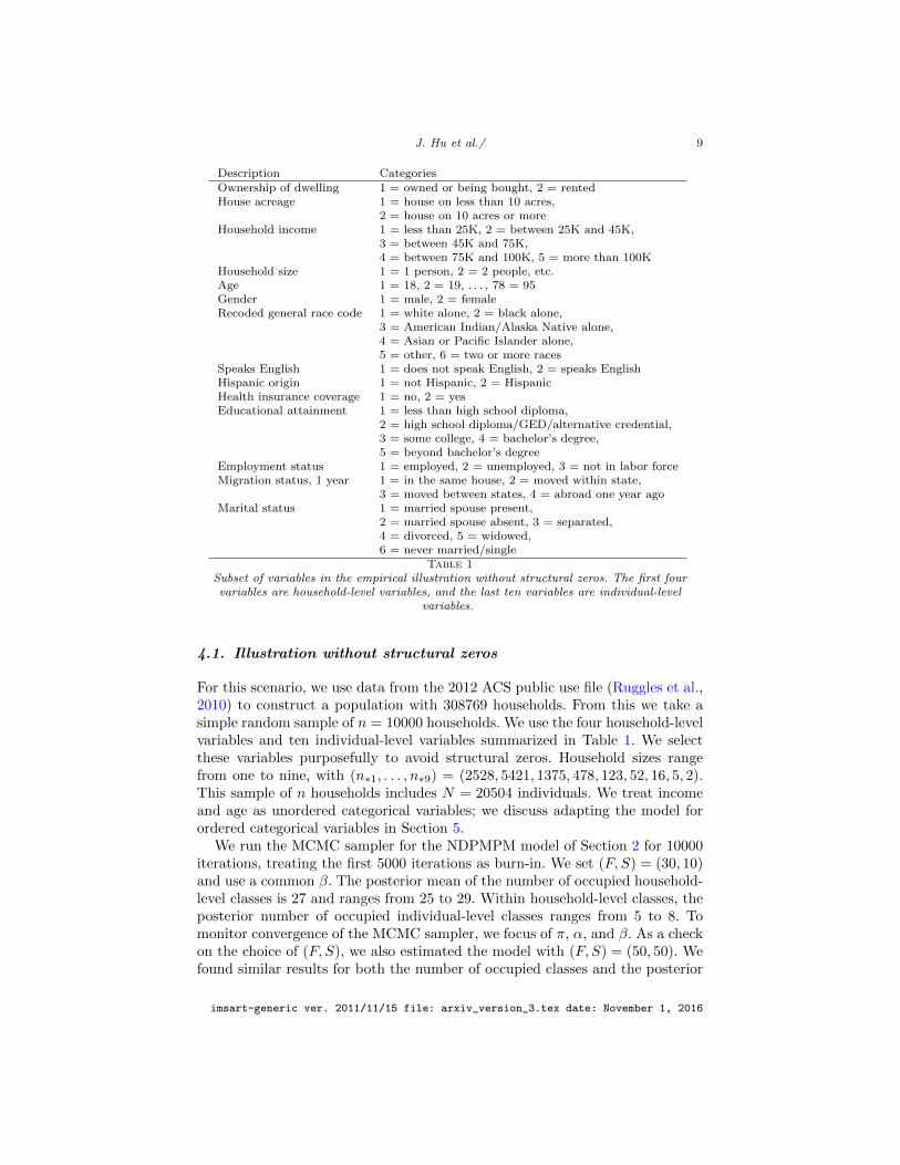
Description CategoriesOwnership of dwelling 1 = owned or being bought, 2 = rentedHouse acreage 1 = house on less than 10 acres,
2 = house on 10 acres or moreHousehold income 1 = less than 25K, 2 = between 25K and 45K,
3 = between 45K and 75K,4 = between 75K and 100K, 5 = more than 100K
Household size 1 = 1 person, 2 = 2 people, etc.Age 1 = 18, 2 = 19, . . . , 78 = 95Gender 1 = male, 2 = femaleRecoded general race code 1 = white alone, 2 = black alone,
3 = American Indian/Alaska Native alone,4 = Asian or Pacific Islander alone,5 = other, 6 = two or more races
Speaks English 1 = does not speak English, 2 = speaks EnglishHispanic origin 1 = not Hispanic, 2 = HispanicHealth insurance coverage 1 = no, 2 = yesEducational attainment 1 = less than high school diploma,
2 = high school diploma/GED/alternative credential,3 = some college, 4 = bachelor’s degree,5 = beyond bachelor’s degree
Employment status 1 = employed, 2 = unemployed, 3 = not in labor forceMigration status, 1 year 1 = in the same house, 2 = moved within state,
3 = moved between states, 4 = abroad one year agoMarital status 1 = married spouse present,
2 = married spouse absent, 3 = separated,4 = divorced, 5 = widowed,6 = never married/single
Table 1Subset of variables in the empirical illustration without structural zeros. The first fourvariables are household-level variables, and the last ten variables are individual-level
variables.
4.1. Illustration without structural zeros
For this scenario, we use data from the 2012 ACS public use file (Ruggles et al.,2010) to construct a population with 308769 households. From this we take asimple random sample of n = 10000 households. We use the four household-levelvariables and ten individual-level variables summarized in Table 1. We selectthese variables purposefully to avoid structural zeros. Household sizes rangefrom one to nine, with (n∗1, . . . , n∗9) = (2528, 5421, 1375, 478, 123, 52, 16, 5, 2).This sample of n households includes N = 20504 individuals. We treat incomeand age as unordered categorical variables; we discuss adapting the model forordered categorical variables in Section 5.
We run the MCMC sampler for the NDPMPM model of Section 2 for 10000iterations, treating the first 5000 iterations as burn-in. We set (F, S) = (30, 10)and use a common β. The posterior mean of the number of occupied household-level classes is 27 and ranges from 25 to 29. Within household-level classes, theposterior number of occupied individual-level classes ranges from 5 to 8. Tomonitor convergence of the MCMC sampler, we focus of π, α, and β. As a checkon the choice of (F, S), we also estimated the model with (F, S) = (50, 50). Wefound similar results for both the number of occupied classes and the posterior
imsart-generic ver. 2011/11/15 file: arxiv_version_3.tex date: November 1, 2016
J. Hu et al./ 10
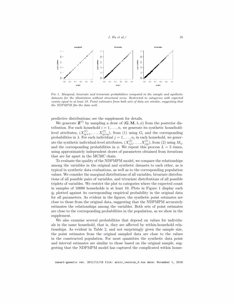
Fig 1. Marginal, bivariate and trivariate probabilities computed in the sample and syntheticdatasets for the illustration without structural zeros. Restricted to categories with expectedcounts equal to at least 10. Point estimates from both sets of data are similar, suggesting thatthe NDPMPM fits the data well.
predictive distributions; see the supplement for details.We generate Z(l) by sampling a draw of (G,M, λ, φ) from the posterior dis-
tribution. For each household i = 1, . . . , n, we generate its synthetic household-
level attributes, (X(l)ip+1, . . . , X
(l)ip+q), from (1) using Gi and the corresponding
probabilities in λ. For each individual j = 1, . . . , ni in each household, we gener-
ate the synthetic individual-level attributes, (X(l)ij1, . . . , X
(l)ijp), from (2) using Mij
and the corresponding probabilities in φ. We repeat this process L = 5 times,using approximately independent draws of parameters obtained from iterationsthat are far apart in the MCMC chain.
To evaluate the quality of the NDPMPM model, we compare the relationshipsamong the variables in the original and synthetic datasets to each other, as istypical in synthetic data evaluations, as well as to the corresponding populationvalues. We consider the marginal distributions of all variables, bivariate distribu-tions of all possible pairs of variables, and trivariate distributions of all possibletriplets of variables. We restrict the plot to categories where the expected countin samples of 10000 households is at least 10. Plots in Figure 1 display eachq5 plotted against its corresponding empirical probability in the original datafor all parameters. As evident in the figures, the synthetic point estimates areclose to those from the original data, suggesting that the NDPMPM accuratelyestimates the relationships among the variables. Both sets of point estimatesare close to the corresponding probabilities in the population, as we show in thesupplement.
We also examine several probabilities that depend on values for individu-als in the same household, that is, they are affected by within-household rela-tionships. As evident in Table 2, and not surprisingly given the sample size,the point estimates from the original sampled data are close to the valuesin the constructed population. For most quantities the synthetic data pointand interval estimates are similar to those based on the original sample, sug-gesting that the NDPMPM model has captured the complicated within house-
imsart-generic ver. 2011/11/15 file: arxiv_version_3.tex date: November 1, 2016
J. Hu et al./ 11
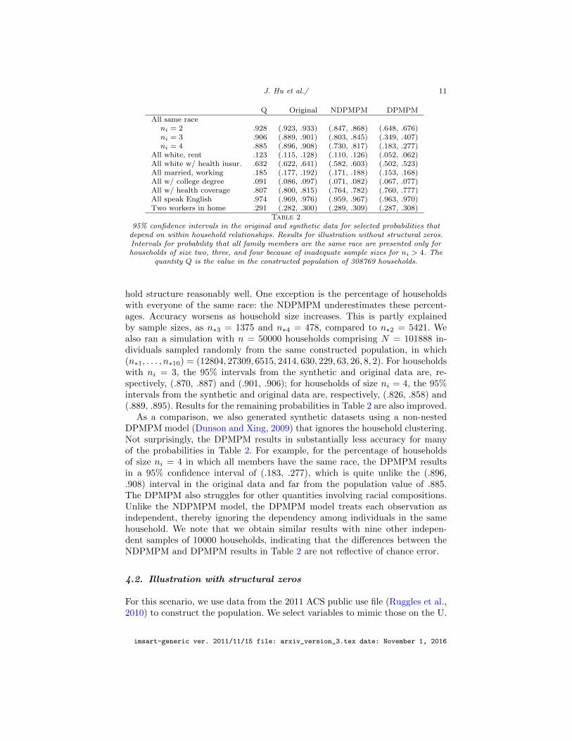
Q Original NDPMPM DPMPMAll same raceni = 2 .928 (.923, .933) (.847, .868) (.648, .676)ni = 3 .906 (.889, .901) (.803, .845) (.349, .407)ni = 4 .885 (.896, .908) (.730, .817) (.183, .277)
All white, rent .123 (.115, .128) (.110, .126) (.052, .062)All white w/ health insur. .632 (.622, .641) (.582, .603) (.502, .523)All married, working .185 (.177, .192) (.171, .188) (.153, .168)All w/ college degree .091 (.086, .097) (.071, .082) (.067, .077)All w/ health coverage .807 (.800, .815) (.764, .782) (.760, .777)All speak English .974 (.969, .976) (.959, .967) (.963, .970)Two workers in home .291 (.282, .300) (.289, .309) (.287, .308)
Table 295% confidence intervals in the original and synthetic data for selected probabilities that
depend on within household relationships. Results for illustration without structural zeros.Intervals for probability that all family members are the same race are presented only forhouseholds of size two, three, and four because of inadequate sample sizes for ni > 4. The
quantity Q is the value in the constructed population of 308769 households.
hold structure reasonably well. One exception is the percentage of householdswith everyone of the same race: the NDPMPM underestimates these percent-ages. Accuracy worsens as household size increases. This is partly explainedby sample sizes, as n∗3 = 1375 and n∗4 = 478, compared to n∗2 = 5421. Wealso ran a simulation with n = 50000 households comprising N = 101888 in-dividuals sampled randomly from the same constructed population, in which(n∗1, . . . , n∗10) = (12804, 27309, 6515, 2414, 630, 229, 63, 26, 8, 2). For householdswith ni = 3, the 95% intervals from the synthetic and original data are, re-spectively, (.870, .887) and (.901, .906); for households of size ni = 4, the 95%intervals from the synthetic and original data are, respectively, (.826, .858) and(.889, .895). Results for the remaining probabilities in Table 2 are also improved.
As a comparison, we also generated synthetic datasets using a non-nestedDPMPM model (Dunson and Xing, 2009) that ignores the household clustering.Not surprisingly, the DPMPM results in substantially less accuracy for manyof the probabilities in Table 2. For example, for the percentage of householdsof size ni = 4 in which all members have the same race, the DPMPM resultsin a 95% confidence interval of (.183, .277), which is quite unlike the (.896,.908) interval in the original data and far from the population value of .885.The DPMPM also struggles for other quantities involving racial compositions.Unlike the NDPMPM model, the DPMPM model treats each observation asindependent, thereby ignoring the dependency among individuals in the samehousehold. We note that we obtain similar results with nine other indepen-dent samples of 10000 households, indicating that the differences between theNDPMPM and DPMPM results in Table 2 are not reflective of chance error.
4.2. Illustration with structural zeros
For this scenario, we use data from the 2011 ACS public use file (Ruggles et al.,2010) to construct the population. We select variables to mimic those on the U.
imsart-generic ver. 2011/11/15 file: arxiv_version_3.tex date: November 1, 2016
J. Hu et al./ 12
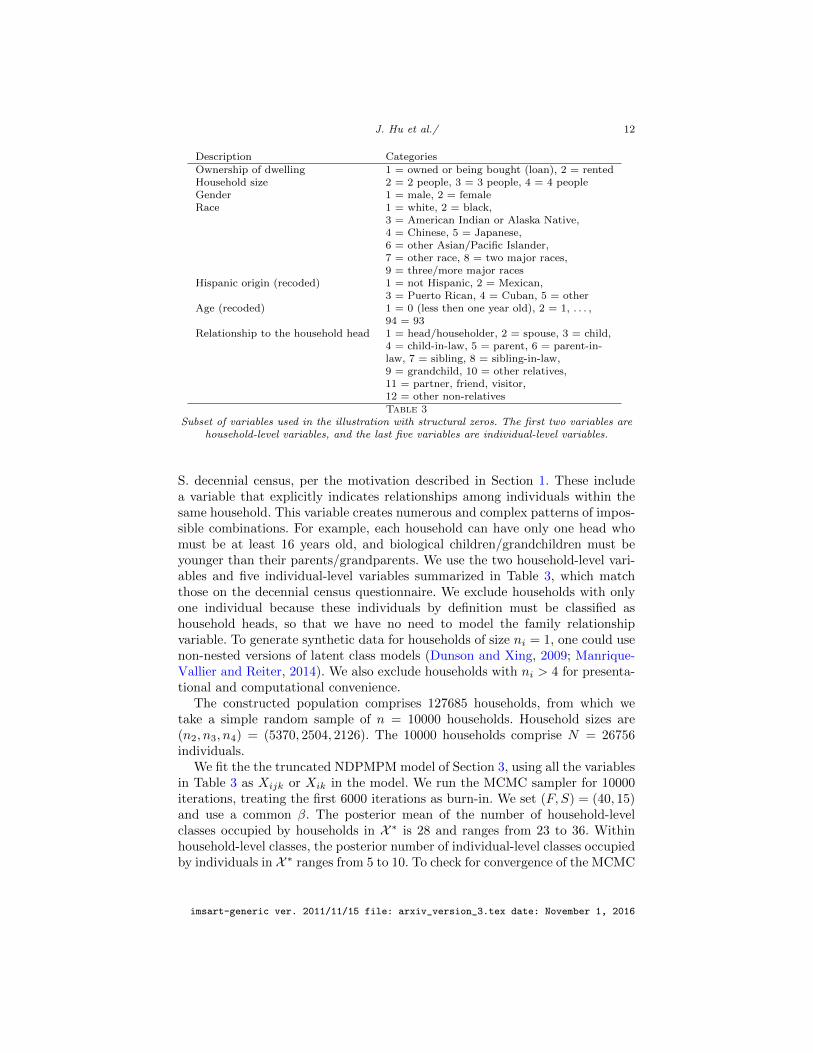
Description CategoriesOwnership of dwelling 1 = owned or being bought (loan), 2 = rentedHousehold size 2 = 2 people, 3 = 3 people, 4 = 4 peopleGender 1 = male, 2 = femaleRace 1 = white, 2 = black,
3 = American Indian or Alaska Native,4 = Chinese, 5 = Japanese,6 = other Asian/Pacific Islander,7 = other race, 8 = two major races,9 = three/more major races
Hispanic origin (recoded) 1 = not Hispanic, 2 = Mexican,3 = Puerto Rican, 4 = Cuban, 5 = other
Age (recoded) 1 = 0 (less then one year old), 2 = 1, . . . ,94 = 93
Relationship to the household head 1 = head/householder, 2 = spouse, 3 = child,4 = child-in-law, 5 = parent, 6 = parent-in-law, 7 = sibling, 8 = sibling-in-law,9 = grandchild, 10 = other relatives,11 = partner, friend, visitor,12 = other non-relativesTable 3
Subset of variables used in the illustration with structural zeros. The first two variables arehousehold-level variables, and the last five variables are individual-level variables.
S. decennial census, per the motivation described in Section 1. These includea variable that explicitly indicates relationships among individuals within thesame household. This variable creates numerous and complex patterns of impos-sible combinations. For example, each household can have only one head whomust be at least 16 years old, and biological children/grandchildren must beyounger than their parents/grandparents. We use the two household-level vari-ables and five individual-level variables summarized in Table 3, which matchthose on the decennial census questionnaire. We exclude households with onlyone individual because these individuals by definition must be classified ashousehold heads, so that we have no need to model the family relationshipvariable. To generate synthetic data for households of size ni = 1, one could usenon-nested versions of latent class models (Dunson and Xing, 2009; Manrique-Vallier and Reiter, 2014). We also exclude households with ni > 4 for presenta-tional and computational convenience.
The constructed population comprises 127685 households, from which wetake a simple random sample of n = 10000 households. Household sizes are(n2, n3, n4) = (5370, 2504, 2126). The 10000 households comprise N = 26756individuals.
We fit the the truncated NDPMPM model of Section 3, using all the variablesin Table 3 as Xijk or Xik in the model. We run the MCMC sampler for 10000iterations, treating the first 6000 iterations as burn-in. We set (F, S) = (40, 15)and use a common β. The posterior mean of the number of household-levelclasses occupied by households in X ∗ is 28 and ranges from 23 to 36. Withinhousehold-level classes, the posterior number of individual-level classes occupiedby individuals in X ∗ ranges from 5 to 10. To check for convergence of the MCMC
imsart-generic ver. 2011/11/15 file: arxiv_version_3.tex date: November 1, 2016
J. Hu et al./ 13
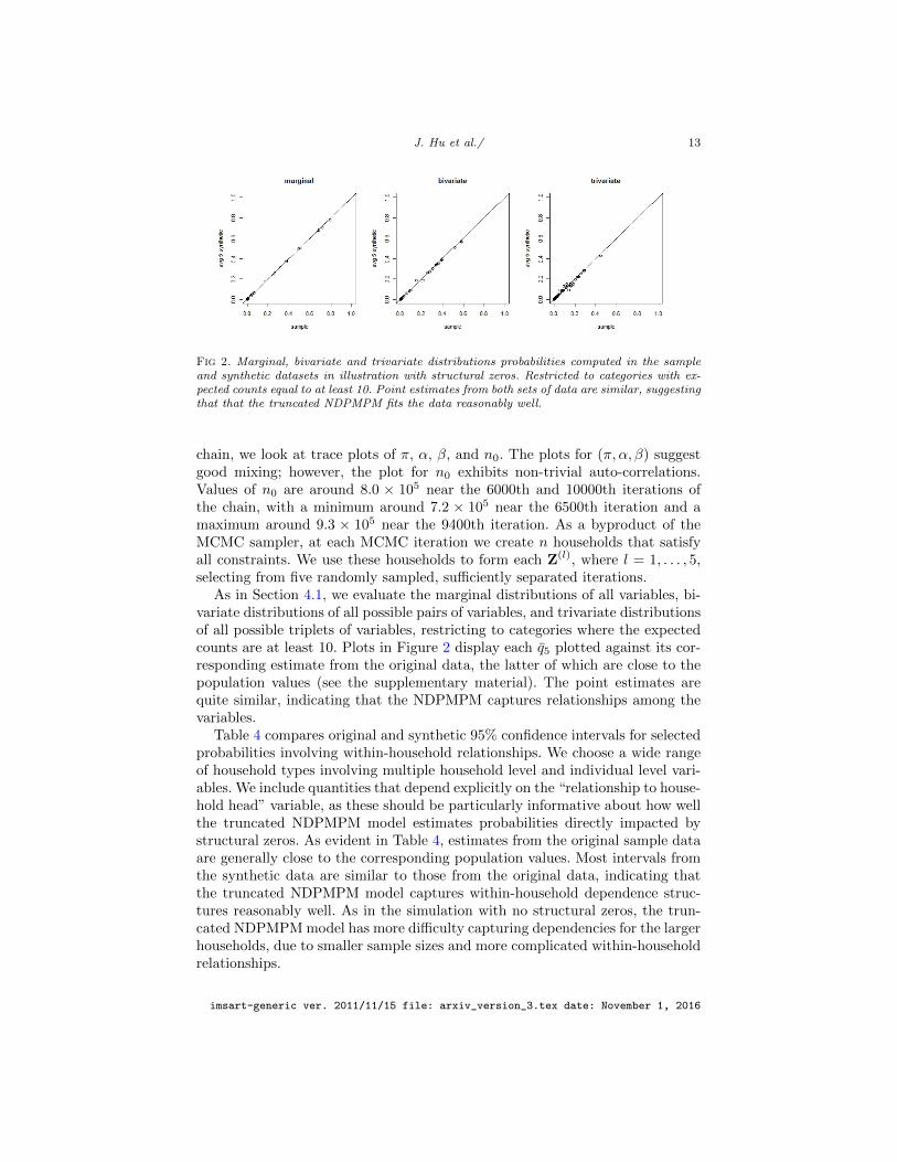
Fig 2. Marginal, bivariate and trivariate distributions probabilities computed in the sampleand synthetic datasets in illustration with structural zeros. Restricted to categories with ex-pected counts equal to at least 10. Point estimates from both sets of data are similar, suggestingthat that the truncated NDPMPM fits the data reasonably well.
chain, we look at trace plots of π, α, β, and n0. The plots for (π, α, β) suggestgood mixing; however, the plot for n0 exhibits non-trivial auto-correlations.Values of n0 are around 8.0 × 10⁵ near the 6000th and 10000th iterations ofthe chain, with a minimum around 7.2 × 10⁵ near the 6500th iteration and amaximum around 9.3 × 10⁵ near the 9400th iteration. As a byproduct of theMCMC sampler, at each MCMC iteration we create n households that satisfyall constraints. We use these households to form each Z(l), where l = 1, . . . , 5,selecting from five randomly sampled, sufficiently separated iterations.
As in Section 4.1, we evaluate the marginal distributions of all variables, bi-variate distributions of all possible pairs of variables, and trivariate distributionsof all possible triplets of variables, restricting to categories where the expectedcounts are at least 10. Plots in Figure 2 display each q5 plotted against its cor-responding estimate from the original data, the latter of which are close to thepopulation values (see the supplementary material). The point estimates arequite similar, indicating that the NDPMPM captures relationships among thevariables.
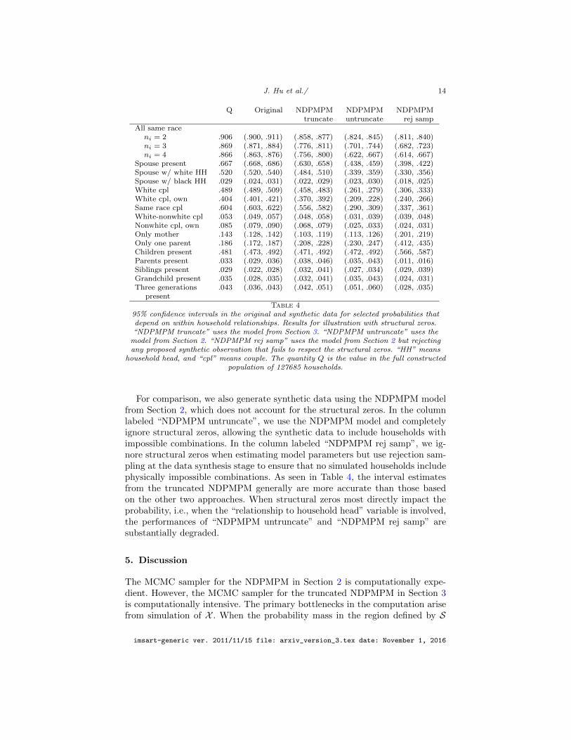
Table 4 compares original and synthetic 95% confidence intervals for selectedprobabilities involving within-household relationships. We choose a wide rangeof household types involving multiple household level and individual level vari-ables. We include quantities that depend explicitly on the “relationship to house-hold head” variable, as these should be particularly informative about how wellthe truncated NDPMPM model estimates probabilities directly impacted bystructural zeros. As evident in Table 4, estimates from the original sample dataare generally close to the corresponding population values. Most intervals fromthe synthetic data are similar to those from the original data, indicating thatthe truncated NDPMPM model captures within-household dependence struc-tures reasonably well. As in the simulation with no structural zeros, the trun-cated NDPMPM model has more difficulty capturing dependencies for the largerhouseholds, due to smaller sample sizes and more complicated within-householdrelationships.
imsart-generic ver. 2011/11/15 file: arxiv_version_3.tex date: November 1, 2016
J. Hu et al./ 14
Q Original NDPMPM NDPMPM NDPMPMtruncate untruncate rej samp
All same raceni = 2 .906 (.900, .911) (.858, .877) (.824, .845) (.811, .840)ni = 3 .869 (.871, .884) (.776, .811) (.701, .744) (.682, .723)ni = 4 .866 (.863, .876) (.756, .800) (.622, .667) (.614, .667)
Spouse present .667 (.668, .686) (.630, .658) (.438, .459) (.398, .422)Spouse w/ white HH .520 (.520, .540) (.484, .510) (.339, .359) (.330, .356)Spouse w/ black HH .029 (.024, .031) (.022, .029) (.023, .030) (.018, .025)White cpl .489 (.489, .509) (.458, .483) (.261, .279) (.306, .333)White cpl, own .404 (.401, .421) (.370, .392) (.209, .228) (.240, .266)Same race cpl .604 (.603, .622) (.556, .582) (.290, .309) (.337, .361)White-nonwhite cpl .053 (.049, .057) (.048, .058) (.031, .039) (.039, .048)Nonwhite cpl, own .085 (.079, .090) (.068, .079) (.025, .033) (.024, .031)Only mother .143 (.128, .142) (.103, .119) (.113, .126) (.201, .219)Only one parent .186 (.172, .187) (.208, .228) (.230, .247) (.412, .435)Children present .481 (.473, .492) (.471, .492) (.472, .492) (.566, .587)Parents present .033 (.029, .036) (.038, .046) (.035, .043) (.011, .016)Siblings present .029 (.022, .028) (.032, .041) (.027, .034) (.029, .039)Grandchild present .035 (.028, .035) (.032, .041) (.035, .043) (.024, .031)Three generations .043 (.036, .043) (.042, .051) (.051, .060) (.028, .035)
presentTable 4
95% confidence intervals in the original and synthetic data for selected probabilities thatdepend on within household relationships. Results for illustration with structural zeros.“NDPMPM truncate” uses the model from Section 3. “NDPMPM untruncate” uses the
model from Section 2. “NDPMPM rej samp” uses the model from Section 2 but rejectingany proposed synthetic observation that fails to respect the structural zeros. “HH” means
household head, and “cpl” means couple. The quantity Q is the value in the full constructedpopulation of 127685 households.
For comparison, we also generate synthetic data using the NDPMPM modelfrom Section 2, which does not account for the structural zeros. In the columnlabeled “NDPMPM untruncate”, we use the NDPMPM model and completelyignore structural zeros, allowing the synthetic data to include households withimpossible combinations. In the column labeled “NDPMPM rej samp”, we ig-nore structural zeros when estimating model parameters but use rejection sam-pling at the data synthesis stage to ensure that no simulated households includephysically impossible combinations. As seen in Table 4, the interval estimatesfrom the truncated NDPMPM generally are more accurate than those basedon the other two approaches. When structural zeros most directly impact theprobability, i.e., when the “relationship to household head” variable is involved,the performances of “NDPMPM untruncate” and “NDPMPM rej samp” aresubstantially degraded.
5. Discussion
The MCMC sampler for the NDPMPM in Section 2 is computationally expe-dient. However, the MCMC sampler for the truncated NDPMPM in Section 3is computationally intensive. The primary bottlenecks in the computation arisefrom simulation of X . When the probability mass in the region defined by S
imsart-generic ver. 2011/11/15 file: arxiv_version_3.tex date: November 1, 2016
J. Hu et al./ 15
is large compared to the probability mass in the region defined by C − S, theMCMC can sample many households with impossible combinations before get-ting n feasible ones. Additionally, it can be time consuming to check whether ornot a generated record satisfies all constraints in S. These bottlenecks can beespecially troublesome when ni is large for many households. To reduce runningtimes, one can parallelize many steps in the sampler (which we did not do). Asexamples, the generation of augmented records and the checking of constraintscan be spread over many processors. One also can reduce computation timeby putting an upper bounds on the size of X (that is still much larger thann). Although this results in an approximation to the Gibbs sampler, this stillcould yield reasonable inferences or synthetic datasets, particularly when manyrecords in X end up in clusters with few data points from X ∗.
Conceptually, the methodology can be readily extended to handle other typesof variables. For example, one could replace the multinomial kernels with con-tinuous kernels (e.g., Gaussian distributions) to handle numerical variables. Forordered categorical variables, one could use a probit specification Albert andChib (1993) or the rank likelihood (Hoff, 2009, Ch. 12). For mixed data, onecould use the Bayesian joint model for multivariate continuous and categoricalvariables developed in Murray and Reiter (2016). Evaluating the properties ofsuch models is a topic for future research.
We did not take advantage of prior information when estimating the models.Such information might be known, for example, from other data sources. In-corporating prior information in latent class models is tricky, because we needto do so in a way that does not distort conditional distributions. Schifeling andReiter (2016) presented a simple approach to doing so for non-nested latent classmodels, in which the analyst appends to the original data partially complete,pseudo-observations with empirical frequencies that match the desired prior dis-tribution. If one had prior information on household size jointly with some othervariable, say individuals’ races, one could follow the approach of Schifeling andReiter (2016) and augment the collected data with partially complete house-holds. When the prior information does not include household size, e.g., justa marginal distribution of race, it is not obvious how to incorporate the priorinformation in a principled way.
Like most joint models, the NDPMPM generally is not appropriate for es-timating multivariate distributions with data from complex sampling designs.This is because the model reflects the distributions in the observed data, whichmight be collected by differentially sampling certain subpopulations. When de-sign variables are categorical and are available for the entire population (not justthe sample), analysts can use the NDPMPM as an engine for Bayesian finitepopulation inference (Gelman et al., 2013, Ch. 8). In this case, the analyst in-cludes the design variables in the NDPMPM, uses the implied, estimated condi-tional distribution to impute many copies of the non-sampled records’ unknownsurvey values given the design variables, and computes quantities of interest oneach completed population. These completed-population quantities summarizethe posterior distribution. Absent this information, there is no consensus on the“best” way to incorporate survey weights in Bayesian joint mixture models. Ku-
imsart-generic ver. 2011/11/15 file: arxiv_version_3.tex date: November 1, 2016
J. Hu et al./ 16
nihama et al. (2014) present a computationally convenient approach that usesonly the survey weights for sampled cases. A similar approach could be appliedfor nested categorical data. Evaluating this approach, as well as other adapta-tions of ideas proposed in the literature, is a worthy topic for future research.
The truncated NDPMPM also assumes the observed data do not includeerrors that create theoretically impossible combinations of values. When suchfaulty values are present, analysts should edit and impute corrected values, forexample, using the Fellegi and Holt (1976) paradigm popular with statisticalagencies. Alternatively, one could add a stochastic measurement error modelto the truncated NDPMPM, as done by Kim et al. (2015) for continuous dataand Manrique-Vallier and Reiter (forthcoming) for non-nested categorical data.While conceptually feasible, this is not a trivial extension. The NDPMPM isalready computationally intensive; searching over the huge space of possibleerror localizations could increase the computational burden substantially. Thissuggests one would need alternatives to standard MCMC algorithms for modelfitting.
imsart-generic ver. 2011/11/15 file: arxiv_version_3.tex date: November 1, 2016

J. Hu et al./ 17
Supplementary materials
6. Introduction
Section 2 describes the full conditionals for the Gibbs sampler for both NDPMPMmodels. Section 3 presents a proof that the sampler for the NDPMPM withstructural zeros gives draws from the posterior distribution of θ under the trun-cated model. Sections 4 to 7 present the results of the assessments of disclosurerisks for the synthetic data illustrations in Section 4 of the main text. We de-scribe the methodology for assessing risks in Section 4 and the computationalmethods in Section 5. We summarize the disclosure risk evaluations for the sce-nario without and with structural zeros in Section 6 and Section 7, respectively.Section 8 presents plots of point estimates versus the population values for boththe synthetic and the original sample data, as described in Section 4 of the maintext. Section 9 presents and compares results using an empirical prior and uni-form prior distribution for the multinomial parameters in the no structural zerossimulation. Section 10 presents and compares results using (F, S) = (50, 50) and(F, S) = (30, 10) in the no structural zeros simulation.
7. Full conditional distributions for MCMC samplers
We present the full conditional distributions used in the Gibbs samplers for theversions of the NDPMPM with and without structural zeros. In both presenta-tions, we assume common β for all household-level clusters.
7.1. NDPMPM without structural zeros
- Sample Gi ∈ {1, . . . , F} from a multinomial distribution with sample size oneand probabilities
Pr(Gi = g|−) =πg{∏qk=p+1 λ
(k)gXik
(∏ni
j=1
∑Sm=1 ωgm
∏pk=1 φ
(k)gmXijk
)}∑Ff=1 πf{
∏qk=p+1 λ
(k)fXik
(∏ni
j=1
∑Sm=1 ωfm
∏pk=1 φ
(k)fmXijk
)}.
- Sample Mij ∈ {1, . . . , S} given Gi from a multinomial distribution with samplesize one and probabilities
Pr(Mij = m|−) =ωGim
∏pk=1 φ
(k)GimXijk∑S
s=1 ωGis
∏pk=1 φ
(k)GisXijk
.
imsart-generic ver. 2011/11/15 file: arxiv_version_3.tex date: November 1, 2016
J. Hu et al./ 18
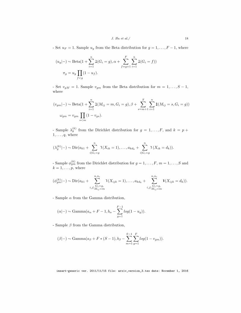
- Set uF = 1. Sample ug from the Beta distribution for g = 1, . . . , F − 1, where
(ug|−) ∼ Beta(1 +
n∑i=1
1(Gi = g), α+
F∑f=g+1
n∑i=1
1(Gi = f))
πg = ug∏f<g
(1− uf ).
- Set vgM = 1. Sample vgm from the Beta distribution for m = 1, . . . , S − 1,where
(vgm|−) ∼ Beta(1 +
n∑i=1
1(Mij = m,Gi = g), β +
S∑s=m+1
n∑i=1
1(Mij = s,Gi = g))
ωgm = vgm∏s<m
(1− vgs).
- Sample λ(k)g from the Dirichlet distribution for g = 1, . . . , F , and k = p +
1, . . . , q, where
(λ(k)g |−) ∼ Dir(ak1 +
n∑i|Gi=g
1(Xik = 1), . . . , akdk +
n∑i|Gi=g
1(Xik = dk)).
- Sample φ(k)gm from the Dirichlet distribution for g = 1, . . . , F , m = 1, . . . , S and
k = 1, . . . , p, where
(φ(k)gm|−) ∼ Dir(ak1 +
n,ni∑i,j| Gi=g,
Mij=m
1(Xijk = 1), . . . , akdk +
n,ni∑i,j| Gi=g,
Mij=m
1(Xijk = dk)).
- Sample α from the Gamma distribution,
(α|−) ∼ Gamma(aα + F − 1, bα −F−1∑g=1
log(1− ug)).
- Sample β from the Gamma distribution,
(β|−) ∼ Gamma(aβ + F ∗ (S − 1), bβ −S−1∑m=1
F∑g=1
log(1− vgm)).
imsart-generic ver. 2011/11/15 file: arxiv_version_3.tex date: November 1, 2016
J. Hu et al./ 19
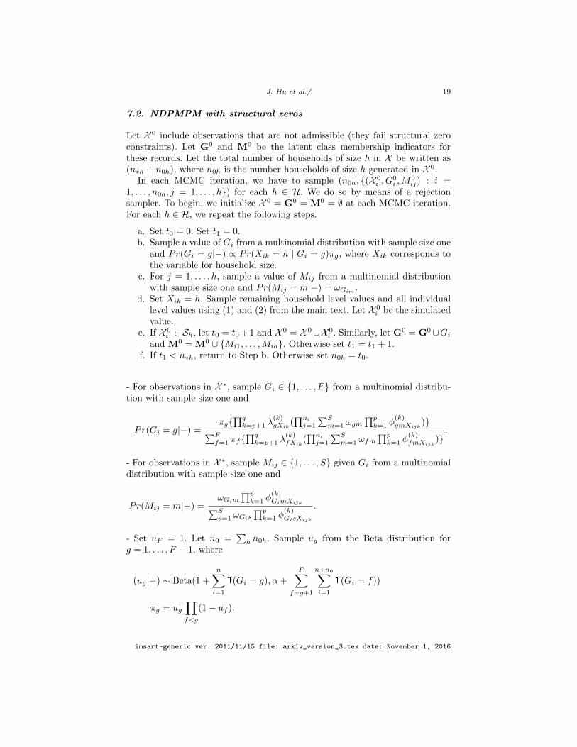
7.2. NDPMPM with structural zeros
Let X 0 include observations that are not admissible (they fail structural zeroconstraints). Let G0 and M0 be the latent class membership indicators forthese records. Let the total number of households of size h in X be written as(n∗h + n0h), where n0h is the number households of size h generated in X 0.
In each MCMC iteration, we have to sample (n0h, {(X 0i , G
0i ,M
0ij) : i =
1, . . . , n0h, j = 1, . . . , h}) for each h ∈ H. We do so by means of a rejectionsampler. To begin, we initialize X 0 = G0 = M0 = ∅ at each MCMC iteration.For each h ∈ H, we repeat the following steps.
a. Set t0 = 0. Set t1 = 0.b. Sample a value of Gi from a multinomial distribution with sample size one
and Pr(Gi = g|−) ∝ Pr(Xik = h | Gi = g)πg, where Xik corresponds tothe variable for household size.
c. For j = 1, . . . , h, sample a value of Mij from a multinomial distributionwith sample size one and Pr(Mij = m|−) = ωGim
.d. Set Xik = h. Sample remaining household level values and all individual
level values using (1) and (2) from the main text. Let X 0i be the simulated
value.e. If X 0
i ∈ Sh, let t0 = t0 + 1 and X 0 = X 0∪X 0i . Similarly, let G0 = G0∪Gi
and M0 = M0 ∪ {Mi1, . . . ,Mih}. Otherwise set t1 = t1 + 1.f. If t1 < n∗h, return to Step b. Otherwise set n0h = t0.
- For observations in X ∗, sample Gi ∈ {1, . . . , F} from a multinomial distribu-tion with sample size one and
Pr(Gi = g|−) =πg{∏qk=p+1 λ
(k)gXik
(∏ni
j=1
∑Sm=1 ωgm
∏pk=1 φ
(k)gmXijk
)}∑Ff=1 πf{
∏qk=p+1 λ
(k)fXik
(∏ni
j=1
∑Sm=1 ωfm
∏pk=1 φ
(k)fmXijk
)}.
- For observations in X ∗, sample Mij ∈ {1, . . . , S} given Gi from a multinomialdistribution with sample size one and
Pr(Mij = m|−) =ωGim
∏pk=1 φ
(k)GimXijk∑S
s=1 ωGis
∏pk=1 φ
(k)GisXijk
.
- Set uF = 1. Let n0 =∑h n0h. Sample ug from the Beta distribution for
g = 1, . . . , F − 1, where
(ug|−) ∼ Beta(1 +
n∑i=1
1(Gi = g), α+
F∑f=g+1
n+n0∑i=1
1(Gi = f))
πg = ug∏f<g
(1− uf ).
imsart-generic ver. 2011/11/15 file: arxiv_version_3.tex date: November 1, 2016

J. Hu et al./ 20
- Set vgM = 1. Sample vgm from the Beta distribution for m = 1, . . . , S − 1,where
(vgm|−) ∼ Beta(1 +
n+n0∑i=1
1(Mij = m,Gi = g), β +
S∑s=m+1
n+n0∑i=1
1(Mij = s,Gi = g))
ωgm = vgm∏s<m
(1− vgs).
- Sample λ(k)g from the Dirichlet distribution for g = 1, . . . , F , and k = p +
1, . . . , q, where
(λ(k)g |−) ∼ Dir(ak1 +
n+n0∑i|Gi=g
1(Xik = 1), . . . , akdk +
n+n0∑i|Gi=g
1(Xik = dk)).
- Sample φ(k)gm from the Dirichlet distribution for g = 1, . . . , F , m = 1, . . . , S and
k = 1, . . . , p, where
(φ(k)gm|−) ∼ Dir(ak1 +
n+n0,ni∑i,j| Gi=g,
Mij=m
1(Xijk = 1), . . . , akdk +
n+n0,ni∑i,j| Gi=g,
Mij=m
1(Xijk = dk)).
- Sample α from the Gamma distribution,
(α|−) ∼ Gamma(aα + F − 1, bα −F−1∑g=1
log(1− ug)).
- Sample β from the Gamma distribution,
(β|−) ∼ Gamma(aβ + F ∗ (S − 1), bβ −S−1∑m=1
F∑g=1
log(1− vgm)).
8. Proof that sampler converges to correct distribution in thetruncated model
In this section, we state and prove a result that ensures draws of θ from thesampler in Section 3 of the main text correspond to draws from the posteriordistribution, p(θ|X ∗, T (S)). The proof follows the strategy in Manrique-Vallierand Reiter (2014). A key difference is that our MCMC algorithm proceeds sep-arately for each h, generating households from the untruncated model untilreaching n∗h feasible households.
imsart-generic ver. 2011/11/15 file: arxiv_version_3.tex date: November 1, 2016

J. Hu et al./ 21
We begin by introducing notation for the augmented data, X . Recall that Xis a draw from a NDPMPM model without restrictions, i.e., all combinationsof household and individual variables are allowed. We write X = (X 1,X 0),where X 1 includes observations that are admissible (no structural zeros) andX 0 includes observations that are not admissible (they fail structural zero con-straints).
Each record in X is associated with a household-level and individual-levellatent class assignment. Let G1 = (G1
1, . . . , G1n) and M1 = {(M1
i1, . . . ,M1ini
), i =1, . . . , n} include all the latent class assignments corresponding to householdsand individuals in X 1. Let G0 = (G0
1, . . . , G0n0
) and M0 = {(M0i1, . . . ,M
0ini
), i =1, . . . , n0} include all the latent class assignments corresponding to the n0 casesin X 0.
We seek to prove that one can obtain samples from p(θ|X ∗, T (S)) in thetruncated NDPMPM from a sampler for f(θ,G1,G0,M1,M0,X 0, {n0h : h ∈H} | X 1) under an untruncated NDPMPM model. Put formally, we want toprove the following theorem
Theorem 1: Let X ∗ comprise n randomly sampled households from the trun-cated NDPMPM in (15) of the main text. Let X 1 be generated from the NDPMPMwithout any concern over structural zeros, i.e., the model from Section 2 of themain text, so that no element of X 1 ∈ S. Assume that X ∗ = X 1. Let the priordistribution on each (n∗h + n0h) be p(n∗h + n0h) ∝ 1/(n∗h + n0h). Then,∫
f(θ,G1,G0,M1,M0,X 0, {n0h}|X 1)dX 0dG1dG0dM1dM0d{n0h}
= p(θ | X ∗, T (S)).
(16)
Here, we use integration signs rather than summation signs to simplify notation.Before continuing with the proof, we note that the rejection sampling step in
the algorithm for the truncated NDPMPM is equivalent to sampling each n0hfrom negative binomial distributions. As evident in the proof, this distributionarises when one assumes a specific, improper prior distribution on (n∗h + n0h)that is independent of θ, namely p(n∗h + n0h) ∝ 1/(n∗h + n0h) for each h.This improper prior distribution is used solely for computational convenience,as using other prior distributions would make the full conditional not negativebinomial and hence complicate the sampling of X 0. A similar strategy wasused by Manrique-Vallier and Reiter (2014), who adapted the improper priorsuggested by Meng and Zaslavsky (2002) and O’Malley and Zaslavsky (2008)for sampling from truncated distributions.
Let Gh = {Gi : ni = h} be the household level latent class assignments ofsize h households and Mh = {Mij : ni = h, j = 1, . . . , ni} be the individuallevel latent class assignments associated with members of size h households. Wesplit Gh into G1
h and G0h, representing the values for records in X 1 and in X 0
respectively. We similarly split Mh into M1h and M0
h. Let X 1h = {X 1
i : ni = h},and let X 0
h = {X 0i : ni = h}. We emphasize that X 1 is used in all iterations,
whereas X 0 is generated in each iteration of the MCMC sampler. Using this
imsart-generic ver. 2011/11/15 file: arxiv_version_3.tex date: November 1, 2016
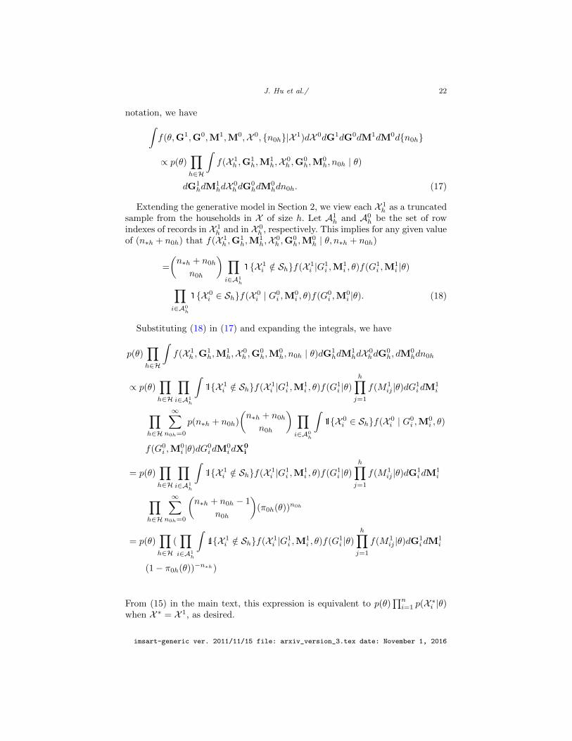
J. Hu et al./ 22
notation, we have∫f(θ,G1,G0,M1,M0,X 0, {n0h}|X 1)dX 0dG1dG0dM1dM0d{n0h}
∝ p(θ)∏h∈H
∫f(X 1
h ,G1h,M
1h,X 0
h ,G0h,M
0h, n0h | θ)
dG1hdM
1hdX 0
hdG0hdM
0hdn0h. (17)
Extending the generative model in Section 2, we view each X 1h as a truncated
sample from the households in X of size h. Let A1h and A0
h be the set of rowindexes of records in X 1
h and in X 0h , respectively. This implies for any given value
of (n∗h + n0h) that f(X 1h ,G
1h,M
1h,X 0
h ,G0h,M
0h | θ, n∗h + n0h)
=
(n∗h + n0h
n0h
) ∏i∈A1
h
1{X 1i /∈ Sh}f(X 1
i |G1i ,M
1i , θ)f(G1
i ,M1i |θ)
∏i∈A0
h
1{X 0i ∈ Sh}f(X 0
i | G0i ,M
0i , θ)f(G0
i ,M0i |θ). (18)
Substituting (18) in (17) and expanding the integrals, we have
p(θ)∏h∈H
∫f(X 1
h ,G1h,M
1h,X 0
h ,G0h,M
0h, n0h | θ)dG1
hdM1hdX 0
hdG0h, dM
0hdn0h
∝ p(θ)∏h∈H
∏i∈A1
h
∫1{X 1
i /∈ Sh}f(X 1i |G1
i ,M1i , θ)f(G1
i |θ)h∏j=1
f(M1ij |θ)dG1
i dM1i
∏h∈H
∞∑n0h=0
p(n∗h + n0h)
(n∗h + n0h
n0h
) ∏i∈A0
h
∫1{X 0
i ∈ Sh}f(X 0i | G0
i ,M0i , θ)
f(G0i ,M
0i |θ)dG0
i dM0i dX
0i
= p(θ)∏h∈H
∏i∈A1
h
∫1{X 1
i /∈ Sh}f(X 1i |G1
i ,M1i , θ)f(G1
i |θ)h∏j=1
f(M1ij |θ)dG1
i dM1i
∏h∈H
∞∑n0h=0
(n∗h + n0h − 1
n0h
)(π0h(θ))n0h
= p(θ)∏h∈H
(∏i∈A1
h
∫1{X 1
i /∈ Sh}f(X 1i |G1
i ,M1i , θ)f(G1
i |θ)h∏j=1
f(M1ij |θ)dG1
i dM1i
(1− π0h(θ))−n∗h)
From (15) in the main text, this expression is equivalent to p(θ)∏ni=1 p(X ∗i |θ)
when X ∗ = X 1, as desired.
imsart-generic ver. 2011/11/15 file: arxiv_version_3.tex date: November 1, 2016
J. Hu et al./ 23
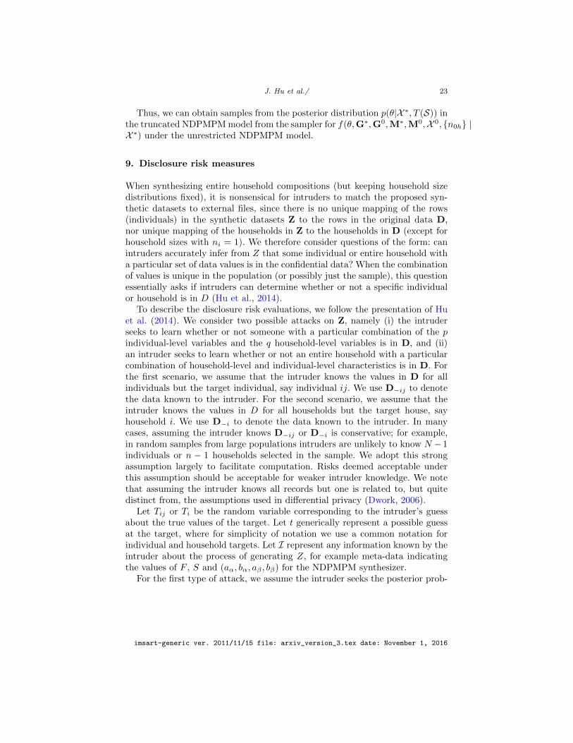
Thus, we can obtain samples from the posterior distribution p(θ|X ∗, T (S)) inthe truncated NDPMPM model from the sampler for f(θ,G∗,G0,M∗,M0,X 0, {n0h} |X ∗) under the unrestricted NDPMPM model.
9. Disclosure risk measures
When synthesizing entire household compositions (but keeping household sizedistributions fixed), it is nonsensical for intruders to match the proposed syn-thetic datasets to external files, since there is no unique mapping of the rows(individuals) in the synthetic datasets Z to the rows in the original data D,nor unique mapping of the households in Z to the households in D (except forhousehold sizes with ni = 1). We therefore consider questions of the form: canintruders accurately infer from Z that some individual or entire household witha particular set of data values is in the confidential data? When the combinationof values is unique in the population (or possibly just the sample), this questionessentially asks if intruders can determine whether or not a specific individualor household is in D (Hu et al., 2014).
To describe the disclosure risk evaluations, we follow the presentation of Huet al. (2014). We consider two possible attacks on Z, namely (i) the intruderseeks to learn whether or not someone with a particular combination of the pindividual-level variables and the q household-level variables is in D, and (ii)an intruder seeks to learn whether or not an entire household with a particularcombination of household-level and individual-level characteristics is in D. Forthe first scenario, we assume that the intruder knows the values in D for allindividuals but the target individual, say individual ij. We use D−ij to denotethe data known to the intruder. For the second scenario, we assume that theintruder knows the values in D for all households but the target house, sayhousehold i. We use D−i to denote the data known to the intruder. In manycases, assuming the intruder knows D−ij or D−i is conservative; for example,in random samples from large populations intruders are unlikely to know N − 1individuals or n − 1 households selected in the sample. We adopt this strongassumption largely to facilitate computation. Risks deemed acceptable underthis assumption should be acceptable for weaker intruder knowledge. We notethat assuming the intruder knows all records but one is related to, but quitedistinct from, the assumptions used in differential privacy (Dwork, 2006).
Let Tij or Ti be the random variable corresponding to the intruder’s guessabout the true values of the target. Let t generically represent a possible guessat the target, where for simplicity of notation we use a common notation forindividual and household targets. Let I represent any information known by theintruder about the process of generating Z, for example meta-data indicatingthe values of F , S and (aα, bα, aβ , bβ) for the NDPMPM synthesizer.
For the first type of attack, we assume the intruder seeks the posterior prob-
imsart-generic ver. 2011/11/15 file: arxiv_version_3.tex date: November 1, 2016
J. Hu et al./ 24
ability,
ρtij = p(Tij = t | Z,D−ij , I) =p(Z | Tij = t,D−ij , I)p(Tij = t | D−ij , I)∑t∈U p(Z | Tij = t,D−ij , I)p(Tij = t | D−ij , I)
(19)
∝ p(Z | Tij = t,D−ij , I)p(Tij = t | D−ij , I), (20)
where U represents the universe of all feasible values of t. Here, p(Z | Tij =t,D−ij , I) is the likelihood of generating the particular set of synthetic datagiven that t is in the confidential data and whatever else is known by the in-truder. The p(Tij = t | D−ij , I) can be considered the intruder’s prior distribu-tion on Tij based on (D−ij , I).
As described in Hu et al. (2014), intruders can use p(Tij = t | Z,D−ij , I) totake guesses at the true value tij . For example, the intruder can find the t thatoffers the largest probability, and use that as a guess of tij . Similarly, agenciescan use p(Tij = t | Z,D−ij , I) in disclosure risk evaluations. For example,for each tij ∈ D, they can rank each t by its associated value of p(Tij = t |Z,D−ij , I), and evaluate the rank at the truth, t = tij . When the rank of tijis high (close to 1, which we define to be the rank associated with the highestprobability), the agency may deem that record to be at risk under the strongintruder knowledge scenario. When the rank of tij is low (far from 1), the agencymay deem the risks for that record to be acceptable.
When U is very large, computing the normalizing constant in (19) is im-practical. To facilitate computation, we follow Hu et al. (2014) and consider asfeasible candidates only those t that differ from tij in one variable, along with tijitself; we call this space Rij . Restricting to Rij can be conceived as mimickinga knowledgeable intruder who searches in spaces near tij . As discussed by Huet al. (2014), restricting support to Rij results in a conservative ranking of thet ∈ Rij , in that ranks determined to be acceptably low when using Rij also areacceptably low when using U .
For Ti, we use a similar approach to risk assessment. We compute
ρti = p(Ti = t | Z,D−i, I) ∝ p(Z | Ti = t,D−i, I)p(Ti = t | D−i, I). (21)
We consider only t that differ from ti in either (i) one household-level variablefor the entire household or (ii) one individual-level variable for one householdmember, along with ti itself; we call this space Ri.
10. Computational methods for risk assessment with the NDPMPMmodel
We describe the computational methods for computing (21) in detail. Methodsfor computing (20) are similar.
For any proposed t, let Dti = (Ti = t,D−i) be the plausible confidential
dataset when Ti = t. Because each Z(l) is generated independently, we have
P (Z | Dti, I) =
L∏l=1
P (Z(l) | Dti, I). (22)
imsart-generic ver. 2011/11/15 file: arxiv_version_3.tex date: November 1, 2016

J. Hu et al./ 25
Hence, we need to compute each P (Z(l) | Dti, I).
Let Θ = {π, ω, λ, φ} denote parameters from a NDPMPM model. We can
write P (Z(l) | Dti, I) as
P (Z(l) | Dti, I) =
∫p(Z(l) | Dt
i, I,Θ)p(Θ | Dti, I)dΘ. (23)
To compute (23), we could sample many values of Θ that could have gener-
ated Z(l); that is, we could sample Θ(r) for r = 1, . . . , R. For each Θ(r), wecompute the probability of generating the released Z(l). We then average theseprobabilities over the R draws of Θ.
Conceptually, to draw Θ replicates, we could re-estimate the NDPMPMmodel for each Dt
i. This quickly becomes computationally prohibitive. Instead,we suggest using the sampled values of Θ from p(Θ | D) as proposals for an im-portance sampling algorithm. To set notation, suppose we seek to estimate theexpectation of some function g(Θ), where Θ has density f(Θ). Further supposethat we have available a sample (Θ(1), . . . ,Θ(R)) from a convenient distributionf∗(Θ) that slightly differs from f(Θ). We can estimate Ef (g(Θ)) using
Ef (g(Θ)) ≈R∑r=1
g(Θ(r))f(Θ(r))/f∗(Θ(r))∑Rr=1 f(Θ(r))/f∗(Θ(r))
. (24)
Let t∗(l)i be the ith household’s values of all variables, including household-
level and individual-level variables, in synthetic dataset Z(l), where i = 1, . . . , nand l = 1, . . . , L. For each Z(l) and any proposed t, we define the g(Θ) in (24)
to equal cP (Z(l) | Dti, I). We approximate the expectation of each g(Θ) with
respect to f(Θ) = f(Θ | Dti, I). In doing so, for any sampled Θ(r) we use
g(Θ(r)) = P (Z(l) | Dti, I,Θ(r)) =
n∏i=1
F∑g=1
π(r)g {
p+q∏k=p+1
λ(k)(r)
gt∗(l)ik
(
ni∏j=1
S∑m=1
ω(r)gm
p∏k=1
φ(k)(r)
gmt∗(l)ijk
)}
.
(25)We set f∗(Θ) = f(Θ | D, I), so that we can use R draws of Θ from its pos-
terior distribution based on D. Let these R draws be (Θ(1), . . . ,Θ(R)). We notethat one could use any Dt
i to obtain the R draws, so that intruders can use simi-lar importance sampling computations. As evident in (1), (2), (3) and (4) in themain text, the only differences in the kernels of f(Θ) and f∗(Θ) include (i) thecomponents of the likelihood associated with record i and (ii) the normalizingconstant for each density. Let t = {(cp+1, . . . , cp+q), (cj1, . . . , cjp), j = 1, . . . , ni},where each ck ∈ (1, . . . , dk), be a guess at Ti, for household-level and individual-level variables respectively. After computing the normalized ratio in (24) andcanceling common terms from the numerator and denominator, we are left withP (Z(l) | Dt
i, I) =∑Rr=1 prqr where
imsart-generic ver. 2011/11/15 file: arxiv_version_3.tex date: November 1, 2016
J. Hu et al./ 26
pr =
n∏i=1
F∑g=1
π(r)g {
p+q∏k=p+1
λ(k)(r)
gt∗(l)ik
(
ni∏j=1
S∑m=1
ω(r)gm
p∏k=1
φ(k)(r)
gmt∗(l)ijk
)}
(26)
qr =
∑F
g=1π(r)g {∏p+q
k=p+1λ(k)(r)gck
(∏ni
j=1
∑S
m=1ω(r)
gm
∏p
k=1φ(k)(r)gmejk
)}∑F
g=1π(r)g {∏p+q
k=p+1λ(k)(r)gtik
(∏ni
j=1
∑S
m=1ω
(h)gm
∏p
k=1φ(k)(r)gmtijk
)}∑Ru=1
(∑F
g=1π(u)g {∏p+q
k=p+1λ(k)(u)gck
(∏ni
j=1
∑S
m=1ω
(u)gm
∏p
k=1φ(k)(u)gmejk
)}∑F
g=1π(u)g {∏p+q
k=p+1λ(k)(u)gtik
(∏ni
j=1
∑S
m=1ω
(u)gm
∏p
k=1φ(k)(u)gmtijk
)}
) .(27)
We repeat this computation for each Z(l), plugging the L results into (22).Finally, to approximate ρti, we compute (22) for each t ∈ Ri, multiplying
each resulting value by its associated P (Ti = t | D−i, I). In what follows, wepresume an intruder with a uniform prior distribution over the support t ∈ Ri.In this case, the prior probabilities cancel from the numerator and denominatorof (19), so that risk evaluations are based only on the likelihood function for Z.We discuss evaluation of other prior distributions in the illustrative application.
For risk assessment for Tij in (20), we use a similar importance samplingapproximation, resulting in
qr =
∑F
g=1π(r)g {∏p+q
k=p+1λ(k)(r)gck
(∑S
m=1ω(r)
gm
∏p
k=1φ(k)(h)gmejk
)}∑F
g=1π(r)g {∏p+q
k=p+1λ(k)(h)gtik
(∑S
m=1ω
(r)gm
∏p
k=1φ(k)(h)gmtijk
)}∑Ru=1
(∑F
g=1π(u)g {∏p+q
k=p+1λ(k)(u)gck
(∑S
m=1ω
(u)gm
∏p
k=1φ(k)(u)gmejk
)}∑F
g=1π(u)g {∏p+q
k=p+1λ(k)(u)gtik
(∑S
m=1ω
(u)gm
∏p
k=1φ(k)(u)gmtijk
)}
) . (28)
11. Disclosure risk assessments for synthesis without structuralzeros
To evaluate the disclosure risks for individuals, we drop each individual recordin D one at a time. For each individual ij, we compute the resulting ρtij for allt in the reduced support Rij . Here, each Rij is the union of the true tij plusthe 39 other combinations of t obtained by changing one variable in tij to anypossible outcome. For any two records ij and i′j′ such that tij = ti′j′ in D,ρtij = ρti′j′ for any possible t. Thus, we need only compute the set of ρtij for the15280 combinations that appeared in D. We use a uniform prior distributionover all t ∈ Rij , for each record ij.
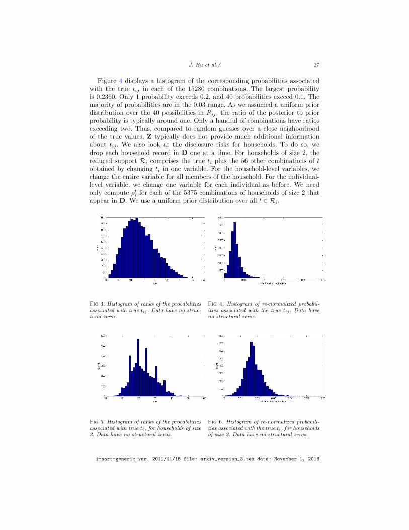
Figure 3 displays the distribution of the rank of the true tij for each of the15280 combinations. Here, a rank equal to 1 means the true tij has the highestprobability of being the unknown Tij , whereas a rank of 40 means the true tij hasthe lowest probability of being Tij . As evident in the figures, even armed withD−ij the intruder gives the top rank to the true tij for only 11 combinations.The intruder gives tij a ranking in the top three for only 194 combinations. Wenote that, even though 12964 combinations were unique in D, the NDPMPMsynthesizer involves enough smoothing that we do not recover the true tij in theoverwhelming majority of cases.
imsart-generic ver. 2011/11/15 file: arxiv_version_3.tex date: November 1, 2016
J. Hu et al./ 27
Figure 4 displays a histogram of the corresponding probabilities associatedwith the true tij in each of the 15280 combinations. The largest probabilityis 0.2360. Only 1 probability exceeds 0.2, and 40 probabilities exceed 0.1. Themajority of probabilities are in the 0.03 range. As we assumed a uniform priordistribution over the 40 possibilities in Rij , the ratio of the posterior to priorprobability is typically around one. Only a handful of combinations have ratiosexceeding two. Thus, compared to random guesses over a close neighborhoodof the true values, Z typically does not provide much additional informationabout tij . We also look at the disclosure risks for households. To do so, wedrop each household record in D one at a time. For households of size 2, thereduced support Ri comprises the true ti plus the 56 other combinations of tobtained by changing ti in one variable. For the household-level variables, wechange the entire variable for all members of the household. For the individual-level variable, we change one variable for each individual as before. We needonly compute ρti for each of the 5375 combinations of households of size 2 thatappear in D. We use a uniform prior distribution over all t ∈ Ri.
Fig 3. Histogram of ranks of the probabilitiesassociated with true tij . Data have no struc-tural zeros.
Fig 4. Histogram of re-normalized probabil-ities associated with the true tij . Data haveno structural zeros.
Fig 5. Histogram of ranks of the probabilitiesassociated with true ti, for households of size2. Data have no structural zeros.
Fig 6. Histogram of re-normalized probabili-ties associated with the true ti, for householdsof size 2. Data have no structural zeros.
imsart-generic ver. 2011/11/15 file: arxiv_version_3.tex date: November 1, 2016
J. Hu et al./ 28
Figure 5 displays the distribution of the rank of the true ti for each of the5375 combinations. Once again, even armed with D−i, the intruder never givesthe top rank to the true ti. the intruder gives the true ti a ranking in thetop three for only seven household combinations. We note that 5331 householdcombinations of size 2 were unique in D.
Figure 6 displays a histogram of the corresponding probabilities associatedwith the true ti in each of the 5375 combinations of households of size 2. Themajority of probabilities are in the 0.02 range. As we assumed a uniform priordistribution over the 57 possibilities in the support, the ratio of the posterior toprior probability is typically around one. Thus, as with individuals, comparedto random guesses over a close neighborhood of the true values, Z typicallydoes not provide much additional information about ti. The largest probabilityis 0.0557.
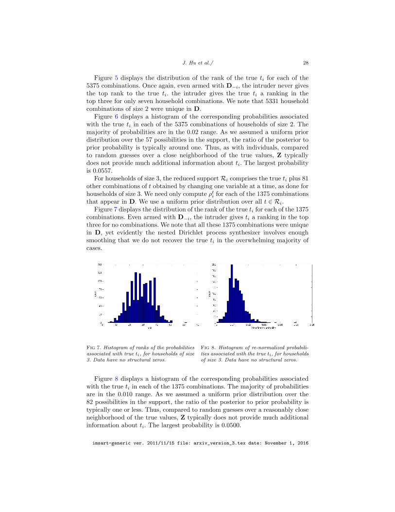
For households of size 3, the reduced support Ri comprises the true ti plus 81other combinations of t obtained by changing one variable at a time, as done forhouseholds of size 3. We need only compute ρti for each of the 1375 combinationsthat appear in D. We use a uniform prior distribution over all t ∈ Ri.
Figure 7 displays the distribution of the rank of the true ti for each of the 1375combinations. Even armed with D−i, the intruder gives ti a ranking in the topthree for no combinations. We note that all these 1375 combinations were uniquein D, yet evidently the nested Dirichlet process synthesizer involves enoughsmoothing that we do not recover the true ti in the overwhelming majority ofcases.
Fig 7. Histogram of ranks of the probabilitiesassociated with true ti, for households of size3. Data have no structural zeros.
Fig 8. Histogram of re-normalized probabili-ties associated with the true ti, for householdsof size 3. Data have no structural zeros.
Figure 8 displays a histogram of the corresponding probabilities associatedwith the true ti in each of the 1375 combinations. The majority of probabilitiesare in the 0.010 range. As we assumed a uniform prior distribution over the82 possibilities in the support, the ratio of the posterior to prior probability istypically one or less. Thus, compared to random guesses over a reasonably closeneighborhood of the true values, Z typically does not provide much additionalinformation about ti. The largest probability is 0.0500.
imsart-generic ver. 2011/11/15 file: arxiv_version_3.tex date: November 1, 2016
J. Hu et al./ 29
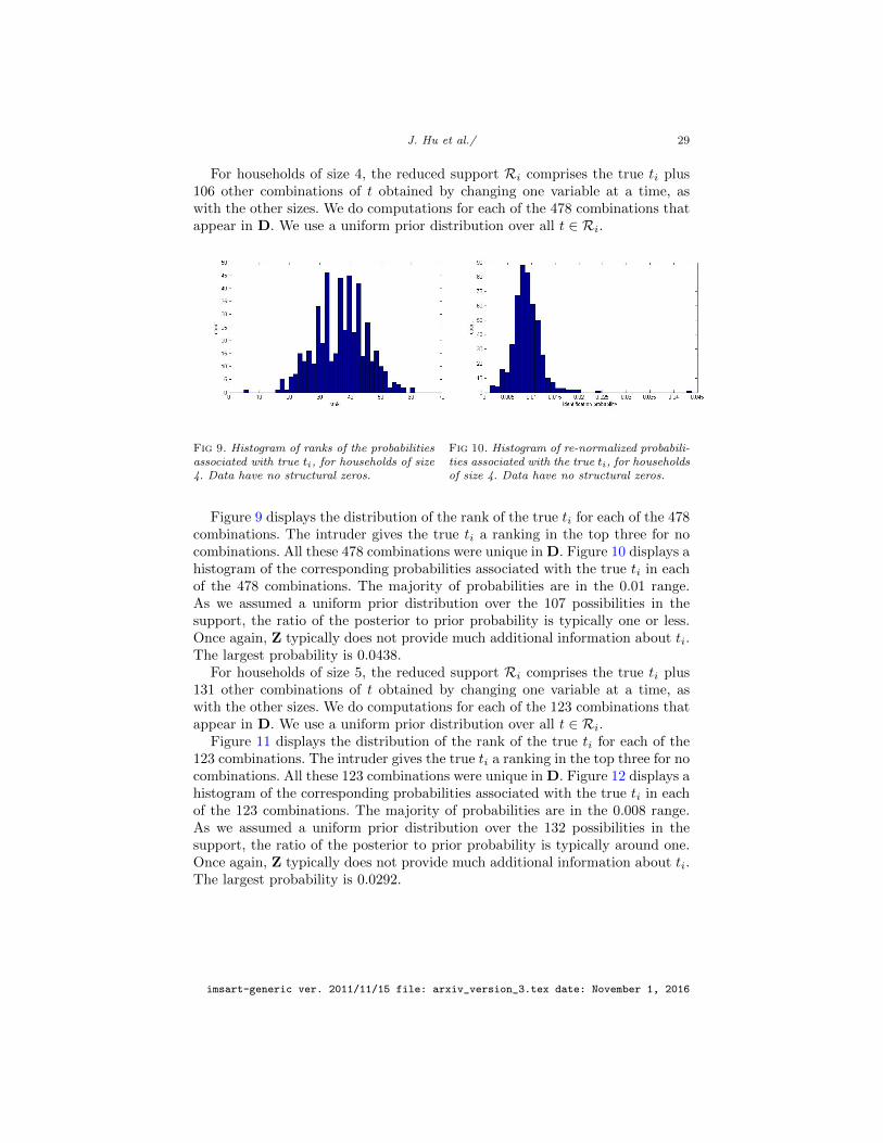
For households of size 4, the reduced support Ri comprises the true ti plus106 other combinations of t obtained by changing one variable at a time, aswith the other sizes. We do computations for each of the 478 combinations thatappear in D. We use a uniform prior distribution over all t ∈ Ri.
Fig 9. Histogram of ranks of the probabilitiesassociated with true ti, for households of size4. Data have no structural zeros.
Fig 10. Histogram of re-normalized probabili-ties associated with the true ti, for householdsof size 4. Data have no structural zeros.
Figure 9 displays the distribution of the rank of the true ti for each of the 478combinations. The intruder gives the true ti a ranking in the top three for nocombinations. All these 478 combinations were unique in D. Figure 10 displays ahistogram of the corresponding probabilities associated with the true ti in eachof the 478 combinations. The majority of probabilities are in the 0.01 range.As we assumed a uniform prior distribution over the 107 possibilities in thesupport, the ratio of the posterior to prior probability is typically one or less.Once again, Z typically does not provide much additional information about ti.The largest probability is 0.0438.
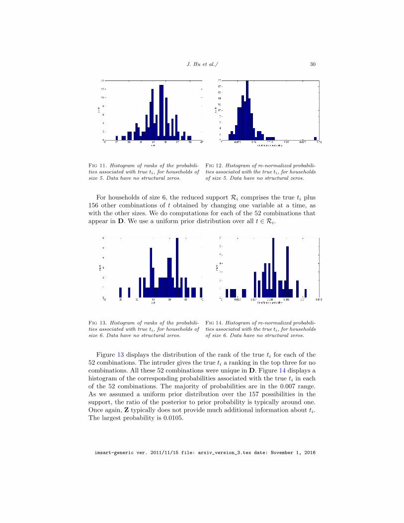
For households of size 5, the reduced support Ri comprises the true ti plus131 other combinations of t obtained by changing one variable at a time, aswith the other sizes. We do computations for each of the 123 combinations thatappear in D. We use a uniform prior distribution over all t ∈ Ri.
Figure 11 displays the distribution of the rank of the true ti for each of the123 combinations. The intruder gives the true ti a ranking in the top three for nocombinations. All these 123 combinations were unique in D. Figure 12 displays ahistogram of the corresponding probabilities associated with the true ti in eachof the 123 combinations. The majority of probabilities are in the 0.008 range.As we assumed a uniform prior distribution over the 132 possibilities in thesupport, the ratio of the posterior to prior probability is typically around one.Once again, Z typically does not provide much additional information about ti.The largest probability is 0.0292.
imsart-generic ver. 2011/11/15 file: arxiv_version_3.tex date: November 1, 2016
J. Hu et al./ 30
Fig 11. Histogram of ranks of the probabili-ties associated with true ti, for households ofsize 5. Data have no structural zeros.
Fig 12. Histogram of re-normalized probabili-ties associated with the true ti, for householdsof size 5. Data have no structural zeros.
For households of size 6, the reduced support Ri comprises the true ti plus156 other combinations of t obtained by changing one variable at a time, aswith the other sizes. We do computations for each of the 52 combinations thatappear in D. We use a uniform prior distribution over all t ∈ Ri.
Fig 13. Histogram of ranks of the probabili-ties associated with true ti, for households ofsize 6. Data have no structural zeros.
Fig 14. Histogram of re-normalized probabili-ties associated with the true ti, for householdsof size 6. Data have no structural zeros.
Figure 13 displays the distribution of the rank of the true ti for each of the52 combinations. The intruder gives the true ti a ranking in the top three for nocombinations. All these 52 combinations were unique in D. Figure 14 displays ahistogram of the corresponding probabilities associated with the true ti in eachof the 52 combinations. The majority of probabilities are in the 0.007 range.As we assumed a uniform prior distribution over the 157 possibilities in thesupport, the ratio of the posterior to prior probability is typically around one.Once again, Z typically does not provide much additional information about ti.The largest probability is 0.0105.
imsart-generic ver. 2011/11/15 file: arxiv_version_3.tex date: November 1, 2016

J. Hu et al./ 31
Fig 15. Histogram of ranks of the probabili-ties associated with true ti, for households ofsize 7. Data have no structural zeros.
Fig 16. Histogram of re-normalized probabili-ties associated with the true ti, for householdsof size 7. Data have no structural zeros.
For households of size 7, the reduced support Ri comprises the true ti plus181 other combinations of t obtained by changing one variable at a time, aswith the other sizes. We do computations for each of the 16 combinations thatappear in D. We use a uniform prior distribution over all t ∈ Ri.
Figure 15 displays the distribution of the rank of the true ti for each of the16 combinations. The intruder gives the true ti a ranking in the top three for nocombinations. All these 16 combinations were unique in D. Figure 16 displays ahistogram of the corresponding probabilities associated with the true ti in eachof the 16 combinations. The majority of probabilities are in the 0.005 range.As we assumed a uniform prior distribution over the 182 possibilities in thesupport, the ratio of the posterior to prior probability is typically around one.Once again, Z typically does not provide much additional information about ti.The largest probability is 0.0083.
For households of size 8, the reduced support Ri comprises the true ti plus206 other combinations of t obtained by changing one variable at a time, as withthe other sizes. We do computations for each of the 5 combinations that appearin D. We use a uniform prior distribution over all t ∈ Ri.
The ranks of the true ti for each of the 5 combinations are {52, 39, 84, 57, 67}.The intruder gives the true ti a ranking in the top three for no combinations.We note that all 5 household combinations of size 8 were unique in D. Thecorresponding probabilities associated with the true ti in each of the 4 combina-tions are {0.0057, 0.0049, 0.0043, 0.0075, 0.0041}. As we assumed a uniform priordistribution over the 207 possibilities in the support, the ratio of the posteriorto prior probability is typically around one. Once again, Z typically does notprovide much additional information about ti. The largest probability is 0.0075.
For households of size 9, the reduced support Ri comprises the true ti plus231 other combinations of t obtained by changing one variable at a time, as withthe other sizes. We do computations for each of the 2 combinations that appearin D. We use a uniform prior distribution over all t ∈ Ri.
The ranks of the true ti for each of the 2 combinations are {57, 66}. Wenote that both 2 household combinations of size 9 were unique in D. The corre-
imsart-generic ver. 2011/11/15 file: arxiv_version_3.tex date: November 1, 2016
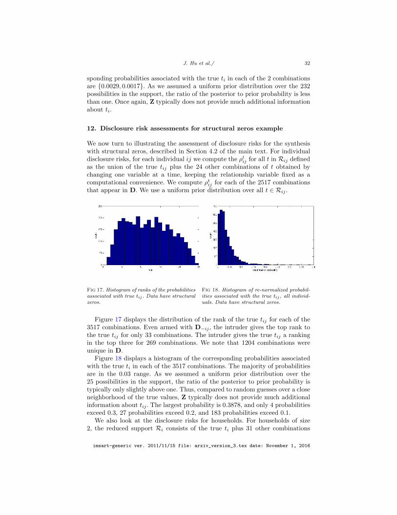
J. Hu et al./ 32
sponding probabilities associated with the true ti in each of the 2 combinationsare {0.0029, 0.0017}. As we assumed a uniform prior distribution over the 232possibilities in the support, the ratio of the posterior to prior probability is lessthan one. Once again, Z typically does not provide much additional informationabout ti.
12. Disclosure risk assessments for structural zeros example
We now turn to illustrating the assessment of disclosure risks for the synthesiswith structural zeros, described in Section 4.2 of the main text. For individualdisclosure risks, for each individual ij we compute the ρtij for all t in Rij definedas the union of the true tij plus the 24 other combinations of t obtained bychanging one variable at a time, keeping the relationship variable fixed as acomputational convenience. We compute ρtij for each of the 2517 combinationsthat appear in D. We use a uniform prior distribution over all t ∈ Rij .
Fig 17. Histogram of ranks of the probabilitiesassociated with true tij . Data have structuralzeros.
Fig 18. Histogram of re-normalized probabil-ities associated with the true tij , all individ-uals. Data have structural zeros.
Figure 17 displays the distribution of the rank of the true tij for each of the3517 combinations. Even armed with D−ij , the intruder gives the top rank tothe true tij for only 33 combinations. The intruder gives the true tij a rankingin the top three for 269 combinations. We note that 1204 combinations wereunique in D.
Figure 18 displays a histogram of the corresponding probabilities associatedwith the true ti in each of the 3517 combinations. The majority of probabilitiesare in the 0.03 range. As we assumed a uniform prior distribution over the25 possibilities in the support, the ratio of the posterior to prior probability istypically only slightly above one. Thus, compared to random guesses over a closeneighborhood of the true values, Z typically does not provide much additionalinformation about tij . The largest probability is 0.3878, and only 4 probabilitiesexceed 0.3, 27 probabilities exceed 0.2, and 183 probabilities exceed 0.1.
We also look at the disclosure risks for households. For households of size2, the reduced support Ri consists of the true ti plus 31 other combinations
imsart-generic ver. 2011/11/15 file: arxiv_version_3.tex date: November 1, 2016

J. Hu et al./ 33
of t obtained by changing ti in one variable. We need only do computationsfor each of the 4070 combinations that appeared in D. We use a uniform priordistribution over all t ∈ Ri.
Figure 19 displays the distribution of the rank of the true ti for each of the4070 combinations. Even armed with D−i, the intruder gives the top rank tothe true ti for no household combination, and gives ti a ranking in the top threefor only 18 combinations. We note that 3485 combinations were unique in D.
Figure 20 displays a histogram of the corresponding probabilities associatedwith the true ti in each of the 4070 combinations. The majority of probabilitiesare in the 0.025 range. As we assumed a uniform prior distribution over the32 possibilities in the support, the ratio of the posterior to prior probability istypically one or less. Thus, compared to random guesses over a reasonably closeneighborhood of the true values, Z typically does not provide much additionalinformation about ti. The largest probability is 0.1740, and only 15 probabilitiesexceed 0.1.
Fig 19. Histogram of ranks of the probabili-ties associated with true ti, for households ofsize 2. Data have structural zeros.
Fig 20. Histogram of re-normalized probabili-ties associated with the true ti, for householdsof size 2. Data have structural zeros.
For households of size 3, the reduced support Ri consists of the true ti plus46 other combinations of t. We need only do computations for each of the 2492combinations that appeared in D. We use a uniform prior distribution over allt ∈ Ri.
Fig 21. Histogram of ranks of the probabili-ties associated with true ti, for households ofsize 3. Data have structural zeros.
imsart-generic ver. 2011/11/15 file: arxiv_version_3.tex date: November 1, 2016
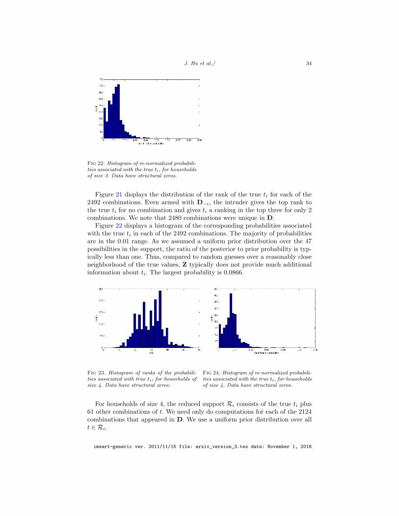
J. Hu et al./ 34
Fig 22. Histogram of re-normalized probabili-ties associated with the true ti, for householdsof size 3. Data have structural zeros.
Figure 21 displays the distribution of the rank of the true ti for each of the2492 combinations. Even armed with D−i, the intruder gives the top rank tothe true ti for no combination and gives ti a ranking in the top three for only 2combinations. We note that 2480 combinations were unique in D.
Figure 22 displays a histogram of the corresponding probabilities associatedwith the true ti in each of the 2492 combinations. The majority of probabilitiesare in the 0.01 range. As we assumed a uniform prior distribution over the 47possibilities in the support, the ratio of the posterior to prior probability is typ-ically less than one. Thus, compared to random guesses over a reasonably closeneighborhood of the true values, Z typically does not provide much additionalinformation about ti. The largest probability is 0.0866.
Fig 23. Histogram of ranks of the probabili-ties associated with true ti, for households ofsize 4. Data have structural zeros.
Fig 24. Histogram of re-normalized probabili-ties associated with the true ti, for householdsof size 4. Data have structural zeros.
For households of size 4, the reduced support Ri consists of the true ti plus61 other combinations of t. We need only do computations for each of the 2124combinations that appeared in D. We use a uniform prior distribution over allt ∈ Ri.
imsart-generic ver. 2011/11/15 file: arxiv_version_3.tex date: November 1, 2016
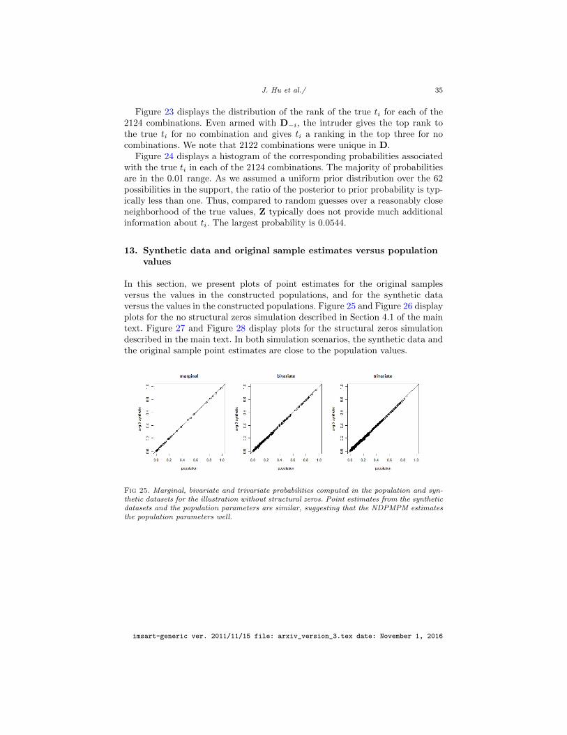
J. Hu et al./ 35
Figure 23 displays the distribution of the rank of the true ti for each of the2124 combinations. Even armed with D−i, the intruder gives the top rank tothe true ti for no combination and gives ti a ranking in the top three for nocombinations. We note that 2122 combinations were unique in D.
Figure 24 displays a histogram of the corresponding probabilities associatedwith the true ti in each of the 2124 combinations. The majority of probabilitiesare in the 0.01 range. As we assumed a uniform prior distribution over the 62possibilities in the support, the ratio of the posterior to prior probability is typ-ically less than one. Thus, compared to random guesses over a reasonably closeneighborhood of the true values, Z typically does not provide much additionalinformation about ti. The largest probability is 0.0544.
13. Synthetic data and original sample estimates versus populationvalues
In this section, we present plots of point estimates for the original samplesversus the values in the constructed populations, and for the synthetic dataversus the values in the constructed populations. Figure 25 and Figure 26 displayplots for the no structural zeros simulation described in Section 4.1 of the maintext. Figure 27 and Figure 28 display plots for the structural zeros simulationdescribed in the main text. In both simulation scenarios, the synthetic data andthe original sample point estimates are close to the population values.
Fig 25. Marginal, bivariate and trivariate probabilities computed in the population and syn-thetic datasets for the illustration without structural zeros. Point estimates from the syntheticdatasets and the population parameters are similar, suggesting that the NDPMPM estimatesthe population parameters well.
imsart-generic ver. 2011/11/15 file: arxiv_version_3.tex date: November 1, 2016
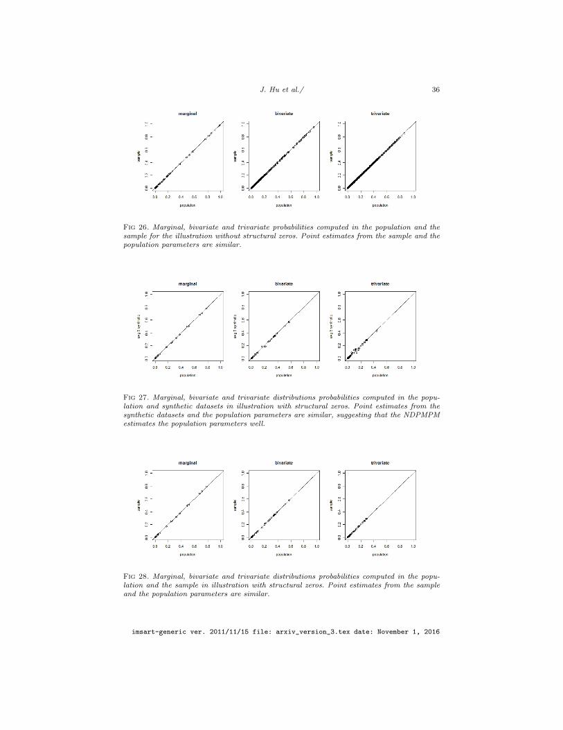
J. Hu et al./ 36
Fig 26. Marginal, bivariate and trivariate probabilities computed in the population and thesample for the illustration without structural zeros. Point estimates from the sample and thepopulation parameters are similar.
Fig 27. Marginal, bivariate and trivariate distributions probabilities computed in the popu-lation and synthetic datasets in illustration with structural zeros. Point estimates from thesynthetic datasets and the population parameters are similar, suggesting that the NDPMPMestimates the population parameters well.
Fig 28. Marginal, bivariate and trivariate distributions probabilities computed in the popu-lation and the sample in illustration with structural zeros. Point estimates from the sampleand the population parameters are similar.
imsart-generic ver. 2011/11/15 file: arxiv_version_3.tex date: November 1, 2016
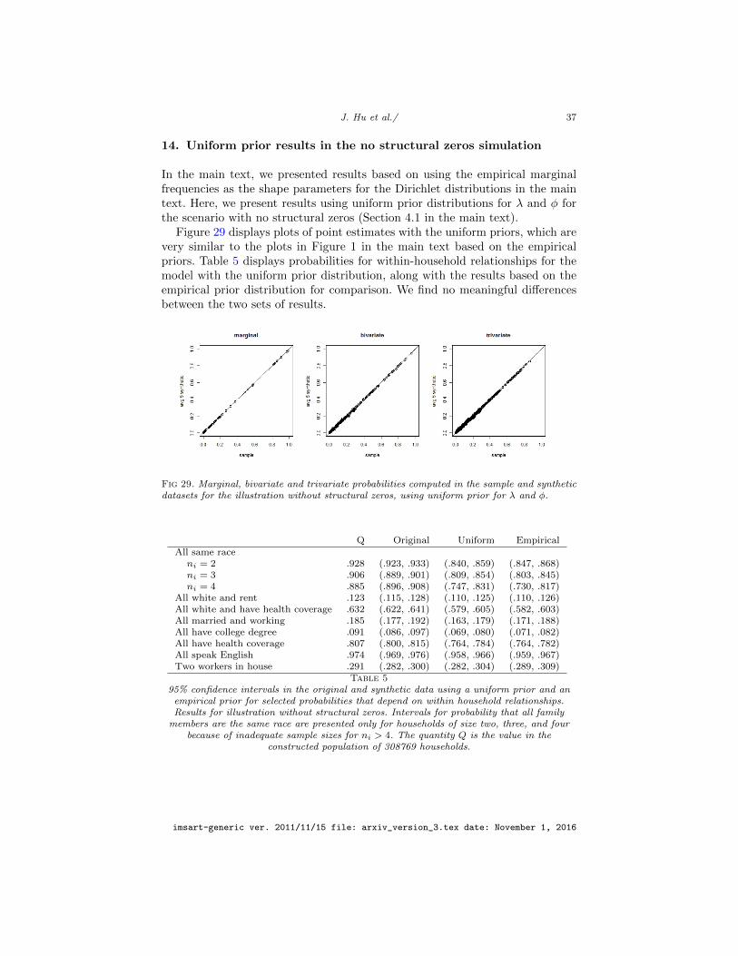
J. Hu et al./ 37
14. Uniform prior results in the no structural zeros simulation
In the main text, we presented results based on using the empirical marginalfrequencies as the shape parameters for the Dirichlet distributions in the maintext. Here, we present results using uniform prior distributions for λ and φ forthe scenario with no structural zeros (Section 4.1 in the main text).
Figure 29 displays plots of point estimates with the uniform priors, which arevery similar to the plots in Figure 1 in the main text based on the empiricalpriors. Table 5 displays probabilities for within-household relationships for themodel with the uniform prior distribution, along with the results based on theempirical prior distribution for comparison. We find no meaningful differencesbetween the two sets of results.
Fig 29. Marginal, bivariate and trivariate probabilities computed in the sample and syntheticdatasets for the illustration without structural zeros, using uniform prior for λ and φ.
Q Original Uniform EmpiricalAll same raceni = 2 .928 (.923, .933) (.840, .859) (.847, .868)ni = 3 .906 (.889, .901) (.809, .854) (.803, .845)ni = 4 .885 (.896, .908) (.747, .831) (.730, .817)
All white and rent .123 (.115, .128) (.110, .125) (.110, .126)All white and have health coverage .632 (.622, .641) (.579, .605) (.582, .603)All married and working .185 (.177, .192) (.163, .179) (.171, .188)All have college degree .091 (.086, .097) (.069, .080) (.071, .082)All have health coverage .807 (.800, .815) (.764, .784) (.764, .782)All speak English .974 (.969, .976) (.958, .966) (.959, .967)Two workers in house .291 (.282, .300) (.282, .304) (.289, .309)
Table 595% confidence intervals in the original and synthetic data using a uniform prior and an
empirical prior for selected probabilities that depend on within household relationships.Results for illustration without structural zeros. Intervals for probability that all family
members are the same race are presented only for households of size two, three, and fourbecause of inadequate sample sizes for ni > 4. The quantity Q is the value in the
constructed population of 308769 households.
imsart-generic ver. 2011/11/15 file: arxiv_version_3.tex date: November 1, 2016
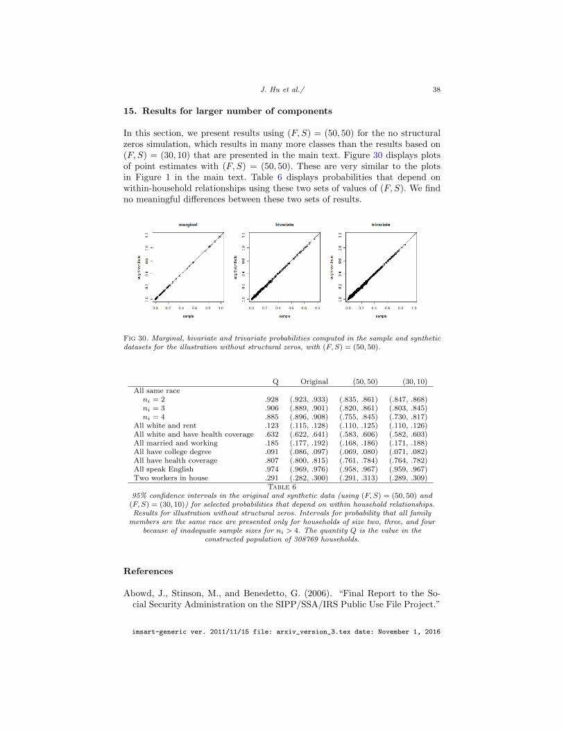
J. Hu et al./ 38
15. Results for larger number of components
In this section, we present results using (F, S) = (50, 50) for the no structuralzeros simulation, which results in many more classes than the results based on(F, S) = (30, 10) that are presented in the main text. Figure 30 displays plotsof point estimates with (F, S) = (50, 50). These are very similar to the plotsin Figure 1 in the main text. Table 6 displays probabilities that depend onwithin-household relationships using these two sets of values of (F, S). We findno meaningful differences between these two sets of results.
Fig 30. Marginal, bivariate and trivariate probabilities computed in the sample and syntheticdatasets for the illustration without structural zeros, with (F, S) = (50, 50).
Q Original (50, 50) (30, 10)All same raceni = 2 .928 (.923, .933) (.835, .861) (.847, .868)ni = 3 .906 (.889, .901) (.820, .861) (.803, .845)ni = 4 .885 (.896, .908) (.755, .845) (.730, .817)
All white and rent .123 (.115, .128) (.110, .125) (.110, .126)All white and have health coverage .632 (.622, .641) (.583, .606) (.582, .603)All married and working .185 (.177, .192) (.168, .186) (.171, .188)All have college degree .091 (.086, .097) (.069, .080) (.071, .082)All have health coverage .807 (.800, .815) (.761, .784) (.764, .782)All speak English .974 (.969, .976) (.958, .967) (.959, .967)Two workers in house .291 (.282, .300) (.291, .313) (.289, .309)
Table 695% confidence intervals in the original and synthetic data (using (F, S) = (50, 50) and
(F, S) = (30, 10)) for selected probabilities that depend on within household relationships.Results for illustration without structural zeros. Intervals for probability that all family
members are the same race are presented only for households of size two, three, and fourbecause of inadequate sample sizes for ni > 4. The quantity Q is the value in the
constructed population of 308769 households.
References
Abowd, J., Stinson, M., and Benedetto, G. (2006). “Final Report to the So-cial Security Administration on the SIPP/SSA/IRS Public Use File Project.”
imsart-generic ver. 2011/11/15 file: arxiv_version_3.tex date: November 1, 2016

J. Hu et al./ 39
Technical report, U.S. Census Bureau Longitudinal Employer-Household Dy-namics Program. Available at http://www.census.gov/sipp/synth_data.
html.Albert, J. H. and Chib, S. (1993). “Bayesian analysis of binary and polychoto-
mous response data.” Journal of the American Statistical Association, 88:669–679.
Bennink, M., Croon, M. A., Kroon, B., and Vermunt, J. K. (2016). “Micro-macro multilevel latent class models with multiple discrete individual-levelvariables.” Advances in Data Analysis and Classification.
Dunson, D. B. and Xing, C. (2009). “Nonparametric Bayes modeling of mul-tivariate categorical data.” Journal of the American Statistical Association,104: 1042–1051.
Dwork, C. (2006). “Differential privacy.” In 33rd International Colloquium onAutomata, Languages, and Programming, part II , 1–12. Berlin: Springer.
Fellegi, I. P. and Holt, D. (1976). “A systematic approach to automatic edit andimputation.” Journal of the American Statistical Association, 71: 17–35.
Gelman, A., Carlin, J. B., Stern, H. S., Dunson, D. B., Vehtari, A., and Rubin,D. B. (2013). Bayesian Data Analysis. London: Chapman & Hall.
Goodman, L. A. (1974). “Exploratory latent structure analysis using both iden-tifiable and unidentifiable models.” Biometrika, 61: 215–231.
Hawala, S. (2008). “Producing partially synthetic data to avoid disclosure.”In Proceedings of the Joint Statistical Meetings. Alexandria, VA: AmericanStatistical Association.
Hoff, P. D. (2009). A First Course in Bayesian Statistical Methods. New York:Springer.
Hu, J., Reiter, J. P., and Wang, Q. (2014). “Disclosure risk evaluation for fullysynthetic categorical data.” In Domingo-Ferrer, J. (ed.), Privacy in StatisticalDatabases, 185–199. Springer.
Ishwaran, H. and James, L. F. (2001). “Gibbs sampling methods for stick-breaking priors.” Journal of the American Statistical Association, 161–173.
Jain, S. and Neal, R. M. (2007). “Splitting and merging components of a non-conjugate Dirichlet process mixture model.” Bayesian Analysis, 2: 445–472.
Kim, H. J., Cox, L. H., Karr, A. F., Reiter, J. P., and Wang, Q. (2015). “Simulta-neous editing and imputation for continuous data.” Journal of the AmericanStatistical Association, 110: 987–999.
Kinney, S., Reiter, J. P., Reznek, A. P., Miranda, J., Jarmin, R. S., and Abowd,J. M. (2011). “Towards unrestricted public use business microdata: The syn-thetic Longitudinal Business Database.” International Statistical Review , 79:363–384.
Kunihama, T., Herring, A. H., Halpern, C. T., and Dunson, D. B. (2014). “Non-parametric Bayes modeling with sample survey weights.” arXiv:1409.5914 .
Little, R. J. A. (1993). “Statistical analysis of masked data.” Journal of OfficialStatistics, 9: 407–426.
Machanavajjhala, A., Kifer, D., Abowd, J., Gehrke, J., and Vilhuber, L. (2008).“Privacy: Theory meets practice on the map.” In IEEE 24th InternationalConference on Data Engineering , 277–286.
imsart-generic ver. 2011/11/15 file: arxiv_version_3.tex date: November 1, 2016
J. Hu et al./ 40
Manrique-Vallier, D. and Reiter, J. P. (2014). “Bayesian estimation of discretemultivariate latent structure models with strutural zeros.” Journal of Com-putational and Graphical Statistics, 23: 1061 – 1079.
Manrique-Vallier, D. and Reiter, J. P. (forthcoming). “Bayesian simultaneousedit and imputation for multivariate categorical data.” Journal of the Amer-ican Statistical Association, to appear.
Meng, X.-L. and Zaslavsky, A. M. (2002). “Single observation unbiased priors.”The Annals of Statistics, 30: 1345–1375.
Murray, J. S. and Reiter, J. P. (2016). “Multiple imputation of missing cate-gorical and continuous values via Bayesian mixture models with local depen-dence.” Journal of the American Statistical Association.
O’Malley, A. J. and Zaslavsky, A. M. (2008). “Domain-level covariance analy-sis for multilevel survey data with structured nonresponse.” Journal of theAmerican Statistical Association, 103: 1405–1418.
Raghunathan, T. E., Reiter, J. P., and Rubin, D. B. (2003). “Multiple impu-tation for statistical disclosure limitation.” Journal of Official Statistics, 19:1–16.
Reiter, J. and Raghunathan, T. E. (2007). “The multiple adaptations of multipleimputation.” Journal of the American Statistical Association, 102: 1462–1471.
Reiter, J. P. (2003). “Inference for partially synthetic, public use microdatasets.” Survey Methodology , 29: 181–189.
— (2005). “Releasing multiply-imputed, synthetic public use microdata: Anillustration and empirical study.” Journal of the Royal Statistical Society,Series A, 168: 185–205.
Rodriguez, A., Dunson, D. B., and Gelfand, A. E. (2008). “The nested Diricheltprocess.” Journal of the American Statistical Association, 103: 1131–1154.
Rubin, D. B. (1993). “Discussion: Statistical disclosure limitation.” Journal ofOfficial Statistics, 9: 462–468.
Ruggles, S., Alexander, J. T., Genadek, K., Goeken, R., Schroeder, M. B.,and Sobek, M. (2010). “Integrated Public Use Microdata Series: Version5.0 [Machine-readable database].” Minneapolis: University of Minnesota.
Schifeling, T. and Reiter, J. P. (2016). “Incorporating marginal prior informationin latent class models.” Bayesian Analysis, 2: 499–518.
Sethuraman, J. (1994). “A constructive definition of Dirichlet priors.” StatisticaSinica, 4: 639–650.
Si, Y. and Reiter, J. P. (2013). “Nonparametric Bayesian multiple imputation forincomplete categorical variables in large-scale assessment surveys.” Journalof Educational and Behavioral Statistics, 38: 499–521.
Vermunt, J. K. (2003). “Multilevel latent class models.” Sociological Methodol-ogy , 213–239.
— (2008). “Latent class and finite mixture models for multilevel data sets.”Statistical Methods in Medical Research, 33–51.
Wade, S., Mongelluzzo, S., and Petrone, S. (2011). “An enriched conjugate priorfor Bayesian nonparametric inference.” Bayesian Analysis, 6: 359–385.
imsart-generic ver. 2011/11/15 file: arxiv_version_3.tex date: November 1, 2016